mechanism for anaphase b: evaluation of ``slide-and ... papers... · mechanism for anaphase b:...
TRANSCRIPT

Biophysical Journal Volume 108 April 2015 2007–2018 2007
Article
Mechanism for Anaphase B: Evaluation of ‘‘Slide-and-Cluster’’ versus‘‘Slide-and-Flux-or-Elongate’’ Models
Ingrid Brust-Mascher,1 Gul Civelekoglu-Scholey,1 and Jonathan M. Scholey1,*1Department of Molecular and Cell Biology, University of California at Davis, Davis, California
ABSTRACT Elongation of the mitotic spindle during anaphase B contributes to chromosome segregation in many cells. Here,we quantitatively test the ability of two models for spindle length control to describe the dynamics of anaphase B spindle elon-gation using experimental data from Drosophila embryos. In the slide-and-flux-or-elongate (SAFE) model, kinesin-5 motorspersistently slide apart antiparallel interpolar microtubules (ipMTs). During pre-anaphase B, this outward sliding of ipMTs isbalanced by depolymerization of their minus ends at the poles, producing poleward flux, while the spindle maintains a constantlength. Following cyclin B degradation, ipMT depolymerization ceases so the sliding ipMTs can push the poles apart. Thecompeting slide-and-cluster (SAC) model proposes that MTs nucleated at the equator are slid outward by the cooperativeactions of the bipolar kinesin-5 and a minus-end-directed motor, which then pulls the sliding MTs inward and clusters them atthe poles. In assessing both models, we assume that kinesin-5 preferentially cross-links and slides apart antiparallel MTs whilethe MT plus ends exhibit dynamic instability. However, in the SAC model, minus-end-directed motors bind the minus ends ofMTs as cargo and transport them poleward along adjacent, parallel MT tracks, whereas in the SAFE model, all MT minusends that reach the pole are depolymerized by kinesin-13. Remarkably, the results show that within a narrow range of MT dy-namic instability parameters, both models can reproduce the steady-state length and dynamics of pre-anaphase B spindles andthe rate of anaphase B spindle elongation. However, only the SAFE model reproduces the change in MT dynamics observedexperimentally at anaphase B onset. Thus, although both models explain many features of anaphase B in this system, our quan-titative evaluation of experimental data regarding several different aspects of spindle dynamics suggests that the SAFE modelprovides a better fit.
INTRODUCTION
The propagation of all cellular life depends on mitosis, dur-ing which piconewton-scale forces generated by dynamicpolymer ratchets and mitotic motors are used to accuratelyseparate copies of the replicated genome packaged intochromosomes (1,2). During mitosis, chromosomes are sepa-rated by a combination of anaphase A, in which chromo-somes move from the spindle equator toward oppositepoles, and anaphase B, in which the spindle poles moveapart, pulling the chromosomes along with them (1,3,4).Anaphase B requires a precise control of mitotic spindlelength (4,5) because the spindle is maintained at a constantlength during pre-anaphase B (i.e., metaphase and/oranaphase A) and then elongates at a characteristic rate to acharacteristic extent. Two models have been proposed toaccount for the control of mitotic spindle length in twodifferent systems, namely, the slide-and-cluster (SAC)model (6) and the slide-and-flux-or-elongate (SAFE) model(7). These two models are based on a sliding-filamentmechanism driven by kinesin-5 motors, but, as discussed
Submitted November 17, 2014, and accepted for publication March 2, 2015.
*Correspondence: [email protected]
This is an open access article under the CC BY-NC-ND license (http://
creativecommons.org/licenses/by-nc-nd/4.0/).
Editor: Fazoil Ataullakhanov.
� 2015 The Authors
0006-3495/15/04/2007/12 $2.00
below, otherwise differ (8–17). We reasoned that a compar-ison of the ability of the SAFE and SAC models to accountfor the control of spindle length changes associatedwith anaphase B might help to identify common anddistinct principles underlying aspects of mitosis in differentsystems.
The SAFE model was initially proposed to describeanaphaseB inDrosophila embryomitotic spindles (7). Thesespindles assemble by a centrosome-directed mechanismthat can be augmented by chromatin- and augmin-directedMT assembly (18), and then segregate chromosomesusing both anaphase A and B (19,20). Whereas anaphaseA depends on a combined kinesin-13-dependent pacman-flux mechanism (21), we propose that anaphase B dependson a persistent kinesin-5-generated interpolar microtubule(ipMT) sliding-filament mechanism that engages to pushapart the spindle poles when poleward flux is turned off(22). Thus, in pre-anaphase B spindles, the outwardsliding of ipMTs is balanced by the kinesin-13 (KLP10A)-catalyzed depolymerization of their minus ends at thepoles, producing poleward flux (21), and the spindle main-tains a steady length. After cyclin B degradation occurs,however, the MT minus-end capping protein patronin (23)counteracts KLP10A activity at spindle poles to turn offipMT minus-end depolymerization so that poleward flux
http://dx.doi.org/10.1016/j.bpj.2015.03.018

2008 Brust-Mascher et al.
ceases and the outwardly sliding ipMTs can now elongate thespindle (24).
The SAC model was initially proposed to account forcontrol of the constant, steady-state length of metaphasespindles in Xenopus egg extracts (6). These spindlesassemble by a chromatin-directed pathway (25) and canbe induced to separate chromosomes by a flux-based mech-anism (26). In the SAC model, MT nucleation occursaround the chromosomes and then kinesin-5 slides thenucleated antiparallel MTs outward (25,27–29). Aroundthe spindle equator, a minus-end-directed motor (e.g., kine-sin-14 or dynein) accumulates at the minus ends of MTsand helps slide them along neighboring MTs toward theminus end of these MTs, thus assisting kinesin-5 aroundthe spindle equator, but opposing it and clustering MTsnear the poles (6,27). In this model, the spindle length isdetermined by the lifetime of the poleward sliding MTs(which in turn is based on MT dynamic instability param-eters solely at the plus ends) and the rate of poleward trans-port of the MTs.
Xenopus extract spindles are thought to have a differentarchitecture compared with Drosophila embryo mitoticspindles (4,30), so it is perhaps not surprising that theSAC and SAFE models differ. Also, because the SAC modelwas proposed to explain the control of metaphase spindlelength in Xenopus, we were initially skeptical of the ideathat the SAC model could be adapted to anaphase B in flyembryos. On the other hand, recent work has uncoveredunexpected features in common between these two typesof spindle, such as the existence of chromatin- and aug-min-directed MT nucleation mechanisms in Drosophila(18), suggesting that the two models might be more broadlyapplicable than we initially thought. Specifically, wewondered whether both the SAFE and SAC models mightbe able to account for the spindle length changes associatedwith pre-anaphase B and anaphase B in Drosophila embryospindles.
Here, we explored this possibility by using quantitative,computational models to compare the ability of the SACand SAFE models to reproduce all the experimental dataon changes in spindle length and MT dynamics observedusing live-cell imaging, fluorescence recovery after photo-bleaching (FRAP), and fluorescence speckle microscopy(FSM) experiments in the Drosophila embryo mitotic spin-dle as it transitioned from its steady-state pre-anaphase Blength to anaphase B spindle elongation. Both models, aswell as a hybrid SAC-SAFE model, displayed remarkablygood agreement with the experiments, although only theSAFE model fit all of the data.
MATERIALS AND METHODS
Here, we outline the basic features of the two published models together
with the new hybrid model, and compare the models for their ability to
explain spindle length control associated with anaphase B in Drosophila
Biophysical Journal 108(8) 2007–2018
embryo mitosis. They are described in more detail in the Supporting
Material (see Fig. 1). First, we list the similarities and differences between
the SAFE and SAC models.
Major similar features
1. Mitotic spindles are made up of bundles of 50–200 minibundles of four
MTs each (Fig. 1 i).
2. The MT-MT plus-end-directed sliding motor is kinesin-5, characterized
by its free sliding velocity (Vm) and maximal force (Fm). Kinesin-5
cross-links both parallel (p) and antiparallel (ap) MTs into bundles,
displaying a 3-fold preference for the antiparallel polarity pattern
(11,15). When it bundles MTs in the antiparallel orientation, it can slide
them apart. When it bundles MTs in the parallel orientation, it cannot
generate force between them, but it can synchronize the sliding rate of
parallel MTs.
3. Only bundles of MTs that span the entire pole-pole distance with anti-
parallel overlapping MTs, either directly or through interactions with
parallel MTs, can exert force on the poles (Fig. 1 ii).
4. MTs exhibit dynamic instability at their plus ends as described by the
four standard parameters, i.e., the growth and shrinkage velocities, vgand vs, which are both fixed parameters based on experimental data
and a parameter scan, respectively, and the rescue and catastrophe
frequencies, fr and fc, which are variable parameters (31,32).
5. When an MT completely depolymerizes, its assembly is renucleated
in the same half spindle to maintain a constant number of MTs
throughout.
Major differences
1. The assembly of MTs is nucleated throughout the entire spindle in the
SAFE model during both pre-anaphase B and anaphase B. In the SAC
model, during pre-anaphase B MTs are nucleated predominantly around
chromatin at the equator. Anaphase B begins after chromosomes have
moved to the poles of Drosophila embryo mitotic spindles (20), so chro-
matin nucleated-MT assembly can no longer occur exclusively around
the spindle equator. Therefore, during anaphase B, we tested MT nucle-
ation predominantly around the poles or throughout the entire spindle
(Fig. 1 iii).
2. In the SAFE model, the minus ends of poleward sliding MTs are depo-
lymerized at the poles during pre-anaphase-B by a kinesin-13-like
minus-end MT depolymerase that depolymerizes every MT minus end
that reaches the pole and whose rate of depolymerization (vdepoly) is a
fixed parameter (Fig. 1 i). This depolymerization is turned off at
anaphase B onset (Fig. 1 iv). In the SAC model, after anaphase B onset,
the dynamic instability parameters of MT plus ends change so that the
MTs become longer (Fig. 1 iv).
3. In the SAC model, when the nonmotor MT-binding tail of a minus-end-
directed motor (e.g., kinesin-14 or dynein) reaches the minus end of one
MT (its cargo), it can bind by its motor domains to a second parallel MT
track and slide the first MT, minus end leading, away from the spindle
equator, as in the original model (6). These motors cooperate with
kinesin-5 motors to enhance poleward MT transport around the equator,
but act antagonistically to kinesin-5 around the poles (6).
Model outline and core equations
All models considered in this study are based on a force-balance (FB)
approach in which the rate of movement of MTs or the spindle poles is
equal to the net force acting on them divided by their drag coefficient
(7). In all descriptions of the modeling strategy and the model framework
outlined below and further detailed in the Supporting Material, forces

i. MT minibundle
ii. Force-generating minibundles
iii. Nucleation region during pre-anaphase B
Microtubuleminus end plus end
Kinesin-5Minus end directed motor (dynein or kinesin-14)Kinesin-13
Key
iv. Switch to spindle elongation
change in plus end dynamics and nucleation region
stop pole associated minus end depolymerization
L (t)
S (t)
A B
C
FIGURE 1 (A and B) SAC (A) and SAFE (B)
models. To compare the two models, we set up
spindles of 50–200 minibundles, each consisting
of four MTs, overlapping antiparallel in the spindle
equator. (i) In both models, kinesin-5 cross-links
and slides ipMTs apart. In the SAC model (left),
a minus-end-directed motor (kinesin-14 or dynein)
accumulates at the minus ends of MTs and walks
toward the minus end of neighboring MTs; thus,
it helps kinesin-5 in the spindle equator but opposes
it near the poles (6). In the SAFE model, kinesin-13
at the poles depolymerizes MT minus ends during
pre-anaphase B, thus maintaining the spindle at a
steady-state length. (ii) Only minibundles spanning
the spindle from pole to pole can generate force on
the poles. (iii) In the SAC model, nucleation is
higher around the chromosomes and thus around
the equator during pre-anaphase B. In the SAFE
model, nucleation is even along the spindle length.
(iv) Anaphase spindle elongation is initiated by a
change in parameters. For the SAC model, the
dynamic instability of MT plus ends is changed,
so the MTs are longer. In addition, nucleation is
either uniform along the spindle length or higher
around the poles. In the SAFE model, minus-end
depolymerization at the poles is turned off, allow-
ing kinesin-5 to push the poles apart. (C) Simplified
spindle to illustrate the FB equations used in the
SAFE model.
Sliding Filaments in Mitosis 2009
and velocities are positive in the poleward direction. For simplicity, we will
refer to the minus-end-directed motor in all equations as Ncd, and to the
bipolar kinesin as kinesin-5.
The realistic spindle consists of minibundles of four potentially overlap-
ping MTs with two MTs facing in opposite directions (Fig. 1 i), each of
which is referred to as a four-MT minibundle. Such a four-MT minibundle
can generate force on the spindle poles when it spans the pole-pole distance
with an overlapping antiparallel pair, and the antiparallel pair can span the
pole-pole distance either directly or through interactions with parallel MTs
(Fig. 1 ii). Forces on the MTs are generated by plus- and/or minus-end-
directed motors. An average number of motors per unit overlap length or
per minus end are active and generate force on the MTs’ parallel and anti-
parallel overlaps. Because the binding and dissociation of motors to and
from the MTs occur on a millisecond timescale (much faster than the move-
ment rate of the MTs and spindle poles), these kinetics are not explicitly
included. The number of motors changes instantly with changes in the over-
lap length due to sliding and/or MT plus-/minus-end dynamics.
SAFE model
The equations for the SAFE model were previously derived in Brust-
Mascher et al. (7). Essentially, the model consists of a system of coupled
differential equations based on the following set of three core equations
that describe an idealized and simplified spindle formed by a single
pair of antiparallel overlapping MTs, as shown in Fig. 1 C. Both MTs
polymerize/depolymerize at exactly the same rate, with kinesin-5 motors
generating outward forces on the MT antiparallel overlaps, and the MTs’
plus and minus ends undergoing dynamic instability and depolymerization,
respectively:
vpole ¼ VslidingðtÞ � vdepoly
dL
dt¼ 2
�Vpoly=depolyðtÞ � VslidingðtÞ
�
mpolevpole ¼ Ftotal ¼ kap LðtÞFm
�1� VslidingðtÞ
Vmaxkinesin5
� ; (1)
where vpole is the velocity of the pole, Vsliding is the sliding rate of the left-
and right-pole-associated overlapping MTs, L(t) is the antiparallel MTover-
lap at time t, mpole is the drag coefficient of the pole, kap is the number of
kinesin-5 motors per unit antiparallel MToverlap, and vdepoly and Vpoly/depoly
are the MT minus-end depolymerization and the MT plus-end growth or
shrinkage rate resulting from MT dynamic instability, respectively. The
above set of equations is adequate for an oversimplified, highly ordered
spindle (Fig. 1 C). A realistic spindle consists of many four-MT minibun-
dles spanning the region between the spindle poles. Each such bundle
can potentially generate force on the poles according to its set of parallel
and antiparallel overlaps, whereas each MT plus end can undergo dynamic
instability independently of the others. This yields different sliding rates of
MTs due to differences in the overlap lengths and thus the number of motors
Biophysical Journal 108(8) 2007–2018

2010 Brust-Mascher et al.
and the load per motor, and results in rapid and asynchronous changes in
each overlap. We describe the FB equations in such a spindle by a large set
of coupled equations that describe the forces generated on each parallel
and antiparallel MT overlap at each time step, based on the current
spindle architecture. Thus, the force on each parallel and antiparallel
MT overlap is described based on the number of active bound motors
(proportional to the overlap size), assuming that the motor-generated forces
are additive (i.e., with equal load sharing). Kinesin-5 motors stepping on the
ith pair of overlapping MTs moving with velocity Vi2 and V
i3 generate a force
of magnitude f ianti�parallel ¼ kapLiapðtÞFstall
kinesin5ð1� ððVi2 þ Vi
3Þ=2Vmaxkinesin5ÞÞ
on antiparallel overlaps, and a force of magnitude f iparallel ¼ kpLipðtÞ
Fstallkinesin5ððVi
2 � Vi1Þ=2Vmax
kinesin5Þ on MTs moving with velocity Vi1 and Vi
2
on parallel overlaps, where kp is the number of kinesin-5 motors per unit
parallel MT overlap. The total force on the spindle poles is the sum of all
forces on all overlapping arrays ofMTs,Ftotal ¼P
f . Since the spindle poles
and MTs are coupled through the FB equation acting on the spindle poles,
this results in a large set of coupled equations that describe the force across
each MT array spanning the distance between the poles together with the
kinematic and FB equations acting on the poles, depending on the parallel
and antiparallel overlap lengths of MTs at any given time. The solution
to these equations yields the sliding velocities of each spindle MT that con-
tributes to force generation and the velocities of the spindle poles, based on
forces generated bymotors working on parallel and antiparallelMToverlaps
at that time point.
It is important to note that in this model there is no minus-end-directed
motor, but MT minus ends contacting a pole are subject to depolymeriza-
tion according to the activity level of the kinesin-13 MT depolymerase
located around the spindle pole. This depolymerase is active during pre-
anaphase B and inactive during anaphase B (Fig. 1 B).
SAC model
In adapting the SAC model to Drosophila embryo mitosis, we modified the
original model by introducing MT dynamic instability into the simulations.
The general framework of the FB equations for a four-MT minibundle
contacting both the left and right poles (and therefore generating forces
on the poles) is shown in Fig. 1 Ai and described as follows:
FB on the top MTof the four-MT minibundle shown in Fig. 1 Ai (MT 1),
overlapping in parallel with MT 2:
F1parallel ¼ f parallelkinesin5 � fNcd ¼ L1ðtÞkp Fstall
kinesin5
�V2 � V1
Vmaxkinesin5
�
�n FstallNcd
�1� V2 � V1
VmaxNcd
�:
(2)
FB on MT 2 of the four-MT minibundle shown in Fig. 1 Ai, overlapping
parallel with MT 1 and antiparallel with MT 3:
Fdrag ¼ �f parallelkinesin5 þ fNcd þ f anti�parallelkinesin5
hMTv2 ¼ �L1ðtÞkp Fstallkinesin5
�V2 � V1
Vmaxkinesin5
�þ n Fstall
Ncd
��1� V2 � V1
VmaxNcd
�þ L2ðtÞkap Fstall
kinesin5
�1� V2 þ V3
Vmaxkinesin5
� ; (3)
where n is the number of Ncd motors per MT minus end and hMT is the drag
coefficient of an MT.
The FB equations for MTs 3 and 4 are derived similarly.
For each minibundle, these FB equations are complemented with two
kinematic equations:
VL ¼ V1 and VR ¼ V4: (4)
Biophysical Journal 108(8) 2007–2018
We further assume that all forces are additive at the poles, yielding
Xi
F1parallel;i ¼ mpole VL þ hMT
Xi
Vi1 and
Xi
F4parallel;i ¼ mpole VR þ hMT
Xi
Vi4:
(5)
The FB equations for bundles with an antiparallel overlap with one or no
parallel overlaps spanning the pole-pole distance (Fig. 1 Aii, upper and mid-
dle bundles) are derived similarly, and the kinematic equations and the cu-
mulative force exerted on the spindle poles by the MT mini bundles are
described as in Eq. 4, with the appropriate modifications.
Combined model
The combined model (SAC-SAFE) has both the minus-end-directed motor
and a depolymerase at the spindle poles. The FB equations are the same as
in the SAC model, but the kinematic equations are complemented with the
MT minus-end depolymerization rates, as in the SAFE model:
VL ¼ V1 � vdepoly and VR ¼ V4 � vdepoly: (6)
In all three models, MT minibundles that do not span the pole-pole distance
do not contribute to the forces exerted on the poles. The FB equations for
the MTs are derived as above (Eqs. 1 and 2), i.e., forces generated between
parallel and/or antiparallel overlaps are balanced by the drag forces on the
MTs. MTs that do not overlap with their immediate neighbors are assumed
to slide freely at the average rate of sliding of other overlapping MTs in the
quarter of the spindle in which they reside (see Numerical Solutions section
in the Supporting Material for details). In the SAFE and SAC-SAFE
models, MT minus ends that contact the spindle poles are depolymerized
according to the level of activity of the MT depolymerase located around
the spindle poles.
The FB and kinematic equations form a large system of coupled ODEs,
which are solved numerically as described in the Supporting Material, to
recover the time-dependent velocities of the MTs and the spindle poles.
Generation of virtual kymographs
Once a numerical simulation of the dynamics of the spindle pole has been
completed, the positions of the spindle MTs’ plus and minus ends, and the
position of the spindle poles for each time step are stored. To generate vir-
tual kymographs, a segment centered at the spindle equator is defined and
divided into 120-nm-long subregions. The amount of tubulin or the number
of speckles or MT plus/minus ends is determined for each subregion at each
time point and plotted using the built in imagesc function in MATLAB (The
MathWorks, Natick, MA).
To generate tubulin kymographs, the number of MTs in each subregion
and at each time point is determined as that which corresponds to the num-
ber of MTs with segments within the boundary of the subregion. To
generate speckled tubulin kymographs, a number of fiduciary marks
proportional to the rounded length of each MT are selected at random
locations along the lattice of each MT at the initial time step. At each
subsequent time step, the position of each one of these marks is updated
using the instantaneous velocity and position of the MT on which it is
located. If an MT shortens or its minus end is depolymerized beyond a
mark, the mark is eliminated. If an MT grows beyond a certain length,
a new mark is added at a random position between the mark closest to
its plus end, and its plus end. Newly nucleated MTs acquire new marks
as they grow. To generate the FSM kymograph, the total number of
fiduciary marks within the boundaries of each subregion at each time point
is determined. Virtual MT plus- or minus-end kymographs are generated
using the time-dependent positions of the MT plus or minus ends,
respectively.
1.2y
Average spindle length16141210 8 6 4 2 0
spin
dle
leng
th (µ
m)
0 50 100 150 200time (s)
B
A
Sliding Filaments in Mitosis 2011
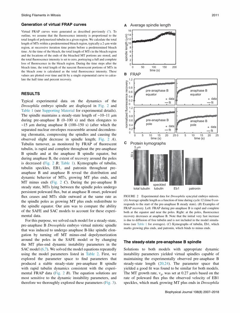
Generation of virtual FRAP curves
Virtual FRAP curves were generated as described previously (7). To
outline, we assume that the fluorescence intensity is proportional to the
total length of polymerized tubulin in a given region. We calculate the total
length of MTs within a predetermined bleach region, typically a 2-mm-wide
region, at successive iteration time points before a predetermined bleach
time. At the time of the bleach, the total length of MTs in the bleach region
and the locations of the ends of the bleached MT portions are stored, and
the total fluorescence intensity is set to zero, portraying a full and complete
loss of fluorescence in the bleach region. During the time steps after the
bleach time, the total length of the nascent fluorescent portions of MTs in
the bleach zone is calculated as the total fluorescence intensity. These
values are plotted over time and fit by a single exponential curve to calcu-
late the half time and percent recovery.
0 5 10 15 20 25
pre-anaphase B equator
pre-anaphase B pole
anaphase B equator
anaphase B pole
00.20.40.60.811.200.20.40.60.81
norm
aliz
ed fl
uore
scen
ce re
cove
r
datafit
datafit
datafit
time (s)
datafit
0 5 10 15 20 25time (s)
total tubulinspeckled tubulin Eb1 patronin
50 s
5 µmC
FIGURE 2 Experimental data for Drosophila syncytial embryo mitosis.
(A) Average spindle length as a function of time during cycle 12 (time 0 cor-
responds to the start of the pre-anaphase B steady state). (B) Examples of
FRAP recovery. Left: FRAP during pre-anaphase B is rapid and complete
both at the equator and near the poles. Right: at the poles, fluorescence
recovery decreases at anaphase B. Note that the initial very fast increase
is due to diffusion of free tubulin and is not included in the model simula-
tions (see Table 1 for averages). (C) Kymographs of tubulin, Eb1, which
marks growing plus ends, and patronin, which binds to minus ends.
RESULTS
Typical experimental data on the dynamics of theDrosophila embryo spindle are displayed in Fig. 2 andTable 1 (see Supporting Material for experimental details).The spindle maintains a steady-state length of ~10–11 mmduring pre-anaphase B (0–100 s) and then elongates to~15 mm during anaphase B (100–150 s) (after which theseparated nuclear envelopes reassemble around decondens-ing chromatin, compressing the spindles and causing theobserved slight decrease in spindle length; Fig. 2 A).Tubulin turnover, as monitored by FRAP of fluorescenttubulin, is rapid and complete throughout the pre-anaphaseB spindle and at the anaphase B spindle equator, butduring anaphase B, the extent of recovery around the polesis decreased (Fig. 2 B; Table 1). Kymographs of tubulin,tubulin speckles, EB1, and patronin throughout pre-anaphase B and anaphase B reveal the distribution anddynamic behavior of MTs, growing MT plus ends, andMT minus ends (Fig. 2 C). During the pre-anaphase Bsteady state, MTs lying between the spindle poles undergopersistent poleward flux, but at anaphase B onset, polewardflux ceases and MTs slide outward at the same rate asthe spindle poles as growing MT plus ends redistribute tothe spindle equator. Our aim was to compare the abilityof the SAFE and SAC models to account for these experi-mental data.
For this purpose, we solved each model for a steady-state,pre-anaphase B Drosophila embryo virtual mitotic spindlethat was induced to undergo anaphase B-like spindle elon-gation by turning off MT minus-end depolymerizationaround the poles in the SAFE model or by changingthe MT plus-end dynamic instability parameters in theSACmodel (6,7). We solved the model equations repeatedlyusing the model parameters listed in Table 2. First, weexplored the parameter space to find parameters thatproduced a stable steady-state pre-anaphase B spindlewith rapid tubulin dynamics consistent with the experi-mental FRAP data (Fig. 2 B). The equation solutions aremost sensitive to the dynamic instability parameters, andtherefore we thoroughly explored these parameters (Fig. 3).
The steady-state pre-anaphase B spindle
Solutions to both models with appropriate dynamicinstability parameters yielded virtual spindles capable ofmaintaining the experimentally observed pre-anaphase Bsteady-state length (20,24). The parameter space thatyielded a good fit was found to be similar for both models.The MT growth rate, vg, was set at 0.27 mm/s based on therate of poleward flux plus the observed velocity of EB1speckles, which mark growing MT plus ends in Drosophila
Biophysical Journal 108(8) 2007–2018

TABLE 1 FRAP parameters for both models (average of 20 runs) versus experimental data
Equator Pole
Half time (s) Percent recovery Half time (s) Percent recovery
Experimental dataa pre-anaphase B 5.3 5 2.0 99 5 7 8.9 5 2.9 96 5 10
N ¼ 56 N ¼ 103
anaphase B 5.0 5 2.8 100 5 11 7.0 5 2.8 86 5 11
N ¼ 31 N ¼ 41
Model
SAFE pre-anaphase B 6.9 5 1.2 102 5 6 9.7 5 2.6 95 5 6
anaphase B 5.9 5 1.4 102 5 8.8 8.7 5 1.9 84 5 10
SAC (higher anaphase B pole nucleation) pre-anaphase B 4.8 5 0.7 99 5 4 9.1 5 3 99 5 19
anaphase B 5.8 5 1 64 5 4 8.3 5 2.9 92 5 9
SAC (even anaphase B nucleation) pre-anaphase B 4.8 5 0.7 99 5 4 9.1 5 3 99 5 19
anaphase B 6.9 5 1.2 81 5 4 14.2 5 2.9 136 5 20
aTubulin FRAP data are biphasic with a fast initial recovery due to diffusion of free tubulin and a second slower phase (see Fig. 2). The models do not consider
free tubulin; therefore, we are comparing the model results with the slower phase of experimental FRAP.
2012 Brust-Mascher et al.
embryo mitotic spindles (33). Then the rate of MTshrinkage, vs, was set at 0.3 mm/s, a value that yielded thelargest range of catastrophe (fc) and rescue (fr) frequencyparameter space to explore for testing the two models.Having set these two parameters, we sought values of fcand fr capable of maintaining a constant spindle lengthand displaying rapid FRAP recovery for the two models,varying these parameters within the ranges shown (Fig. 3,A and B). We find that the dynamic instability parametersused in solving both models have to be fine-tuned (Fig. 3C); otherwise, the spindle collapses, grows, or displaysunrealistic dynamic behavior. Note that for the same rescuefrequency, the range of catastrophe frequencies that givean acceptable fit is slightly lower for the SAFE model(Fig. 3 C). This is because excess MT growth is opposed
TABLE 2 Model parameters
Parameter Value or range tested
Time step (s) 0.5
Number of ipMTs per bundle 10–30
Number of bundles 5–10
Drag coefficients (pN � s/mm)
MT (hMT) 0.5
Pole (mpole) 1000
Dynamic instability parameters
Vgrowth (mm/s) 0.27
Vshrinkage (mm/s) 0.1–0.4
frescue (1/s) 0.02–0.3
fcatastrophe (1/s) 0.02–0.5
Sliding motor
Fm (pN) 1–10
Vm (mm/s) 0.01–0.1
Number of motors per mm of ap overlap, kap 3–300
Number of motors per mm of p overlap, kp 1–100
Minus-end motor
Fm (pN) 1–10
Vm (mm/s) 0.1–1
Number of motors per MT minus end, n 1–300
Minus-end depolymerase at pole
vdepmax (mm/s) preanaphase B 0.01–0.1
vdepmax (mm/s) anaphase B 0
Biophysical Journal 108(8) 2007–2018
by MT minus-end depolymerization, which stabilizes thespindle length. However, the range is not larger becausealthough spindle length is stable for all lower catastrophefrequencies, FRAP recovery is too slow to account for ob-servations of real spindles. The significance of the narrowdynamic instability parameter space is discussed below(see Discussion).
Anaphase B spindle elongation
A key difference between the SAC and SAFE models is thenature of the change in MT polymer dynamics that producesa change in spindle length, being confined to MT plus endsfacing the spindle equator in the former case and to theminus ends around the poles in the latter model (6,7).
Reference SAC model (Fig. 4) SAFE model (Fig. 5)
0.5 0.5
(14) 30 30
(14) 5 5
(34) 0.5 0.5
(35) 1000 1000
(33) 0.27 0.27
0.3 0.3
(36,37) See Fig. 2 and Table 3
(36–38)
(39) 5 5
0.06 0.06
(14,15) 30 30
(14,15) 10 10
(40) 1 N/A
(40) 0.1 N/A
15 N/A
(7) N/A 0.06
N/A 0

0.5
0.45
0.4
0.35
0.3
0.25
0.2
0.15
0.1
0.05
0
cata
stro
phe
frequ
ency
(1/s
)
0.50.450.40.350.30.250.20.150.10.050
cata
stro
phe
frequ
ency
(1/s
)
Slide and clusterSlide and flux-or-elongate
0 0.04 0.08 0.12 0.16 0.2 0.24 0.28rescue frequency (1/s)
0.5
0.45
0.4
0.35
0.3
0.25
0.2
0.15
0.1
0.05
0
cata
stro
phe
frequ
ency
(1/s
)
0 0.04 0.08 0.12 0.16 0.2 0.24 0.28rescue frequency (1/s)
0 0.04 0.08 0.12 0.16 0.2 0.24 0.28rescue frequency (1/s)
C
B
A Slide and cluster
Slide and flux-or-elongate
Working parameter space
FIGURE 3 Steady state in SAC versus SAFE models. (A and B) We
explored the dynamic instability parameter space for the SAC (A) and
SAFE (B) models, looking for parameters that maintain a steady spindle
length and exhibit rapid FRAP recovery both near the poles and at the
equator (vg ¼ 0.27 mm/s, vs ¼ 0.3 mm/s, fr varied from 0.02 to 0.3 /s,
and fc varied from 0.02 to 0.5/s). (C) In both models, the parameters
have to be fine-tuned to maintain a stable spindle with rapid dynamics. If
catastrophe is too high, the spindles collapse (red); in a narrow region the
spindles are stable and exhibit rapid dynamics (blue); and if rescue is too
high, spindles grow in the SAC model (A) or exhibit slow dynamics in
the SAFE model (B) (green).
Sliding Filaments in Mitosis 2013
To determine whether solutions to the SAC model couldaccount for anaphase B spindle dynamics in Drosophilaembryo spindles, we elongated the virtual pre-anaphase Bspindles by changing MT plus-end dynamic instability para-meters by increasing the rescue frequency (fr), lowering thecatastrophe frequency (fc), or using a combination of both.Because anaphase B spindle elongation was not addressedin the originalmodel (6) (and indeed is not a consistent featureof Xenopus extract spindles (26)), we solved the model underconditions in which MT nucleation occurs throughout thespindle during anaphase B, consistent with Drosophilaembryo spindles. The results obtained show that spindle elon-gation at the observed experimental rate is possible (Fig. 4 A,i and ii), although in repeated runs there was variability inthe timing of the initiation of spindle elongation, a featurethat was not shared with real spindles in this system.
Because the SAC model assumes MT nucleation aroundchromatin, and chromosomes have mostly moved to thepoles by anaphase B onset, we also tested higher nucleationat the poles during anaphase B (Fig. 4 B). Coupled with achange in plus-end dynamics, this also leads to spindle elon-gation at the observed rate, again with a delay in the initia-tion of elongation after the parameter change.
In both cases, the spindle elongation extends beyond thatobserved experimentally and therefore yields a larger spin-dle length. In exploring the parameters, we found thatchanging the dynamic instability parameters affected boththe rate and extent of spindle elongation (Fig. S1). Forfurther study, we chose parameters that gave the observedelongation rate, even if the extent of elongation was largerthan that observed in vivo.
To elongate virtual spindles in the SAFE model frame-work, we inhibited MT minus-end depolymerization at thespindle poles and again observed that realistic anaphaseB-like spindle elongation could be produced (Fig. 5, i andii). In this case, in repeated runs, the initiation of spindleelongation was very reproducible. To match the extent ofspindle elongation, we also introduced a small additionalchange in dynamics at the MT plus ends so that the overlaplength was maintained, but this was not necessary for initialspindle elongation at the observed rate (Fig. S2). In the caseof the SAC model, we did not find parameters that yieldedanaphase B spindle elongation that matched both the rateand extent observed experimentally. Only one or the othercondition was satisfied, which may reflect a deficiency ofthe SAC model relative to the SAFE model.
In addition to comparing spindle length versus time plots,we generated virtual FRAP and kymographs displaying thedynamic behavior of total tubulin, fluorescent tubulinspeckles, growing MT plus ends, and minus ends from solu-tions to both models. The spindle length and kymographscorrespond quite well to those obtained from real spindles(compare Figs. 4 and 5 with Fig. 2). However, in the SACmodel, the pre-anaphase B spindle length exhibits morefluctuations and the total tubulin distribution is uneven,
Biophysical Journal 108(8) 2007–2018
i. Average spindle length ii. Example run
iii. In silico FRAP
iv. In silico kymographs
time (s)
pole
pos
ition
(µm
)
time (s)
pre-anaphase B equator
0 10 20 30 40 50time (s)
simulatedfit
total tubulin speckled tubulin
growing plus ends
minus ends
norm
aliz
ed fl
uore
scen
ce re
cove
ry
pre-anaphase B pole
anaphase Bequator
anaphase B pole
8 6 4 2 0-2-4-6-8
0 50 100 150 200
simulatedfit
0 10 20 30 40 50
00.20.40.60.811.21.4
00.20.40.60.811.21.4
simulatedfit
simulatedfit
20
15
10
5
0
spin
dle
leng
th (µ
m)
0 50 100 150 200time (s)
5µm
50s
i. Average spindle length ii. Example run
iii. In silico FRAP
iv. In silico kymographs
time (s)
pole
pos
ition
(µm
)
time (s)
pre-anaphase B equator
0 10 20 30 40 50time (s)
simulatedfit
norm
aliz
ed fl
uore
scen
ce re
cove
ry
pre-anaphase B pole
anaphase Bequator
anaphase B pole
8 6 4 2 0-2-4-6-8
0 50 100 150 200
simulatedfit
0 10 20 30 40 50
00.20.40.60.811.21.4
00.20.40.60.811.21.4
simulatedfit
simulatedfit
20
15
10
5
0
spin
dle
leng
th (µ
m)
0 50 100 150 200time (s)
5µm
50s
A B
total tubulin speckled tubulin
growing plus ends
minus ends
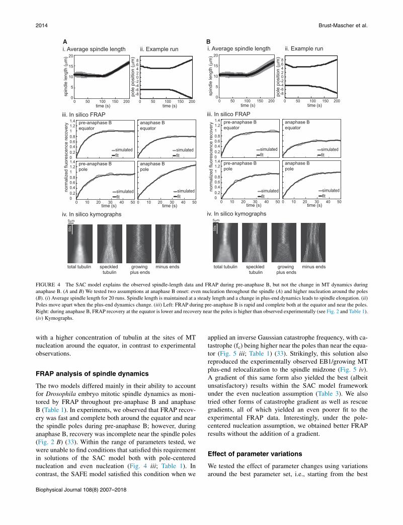
FIGURE 4 The SAC model explains the observed spindle-length data and FRAP during pre-anaphase B, but not the change in MT dynamics during
anaphase B. (A and B) We tested two assumptions at anaphase B onset: even nucleation throughout the spindle (A) and higher nucleation around the poles
(B). (i) Average spindle length for 20 runs. Spindle length is maintained at a steady length and a change in plus-end dynamics leads to spindle elongation. (ii)
Poles move apart when the plus-end dynamics change. (iii) Left: FRAP during pre-anaphase B is rapid and complete both at the equator and near the poles.
Right: during anaphase B, FRAP recovery at the equator is lower and recovery near the poles is higher than observed experimentally (see Fig. 2 and Table 1).
(iv) Kymographs.
2014 Brust-Mascher et al.
with a higher concentration of tubulin at the sites of MTnucleation around the equator, in contrast to experimentalobservations.
FRAP analysis of spindle dynamics
The two models differed mainly in their ability to accountfor Drosophila embryo mitotic spindle dynamics as moni-tored by FRAP throughout pre-anaphase B and anaphaseB (Table 1). In experiments, we observed that FRAP recov-ery was fast and complete both around the equator and nearthe spindle poles during pre-anaphase B; however, duringanaphase B, recovery was incomplete near the spindle poles(Fig. 2 B) (33). Within the range of parameters tested, wewere unable to find conditions that satisfied this requirementin solutions of the SAC model both with pole-centerednucleation and even nucleation (Fig. 4 iii; Table 1). Incontrast, the SAFE model satisfied this condition when we
Biophysical Journal 108(8) 2007–2018
applied an inverse Gaussian catastrophe frequency, with ca-tastrophe (fc) being higher near the poles than near the equa-tor (Fig. 5 iii; Table 1) (33). Strikingly, this solution alsoreproduced the experimentally observed EB1/growing MTplus-end relocalization to the spindle midzone (Fig. 5 iv).A gradient of this same form also yielded the best (albeitunsatisfactory) results within the SAC model frameworkunder the even nucleation assumption (Table 3). We alsotried other forms of catastrophe gradient as well as rescuegradients, all of which yielded an even poorer fit to theexperimental FRAP data. Interestingly, under the pole-centered nucleation assumption, we obtained better FRAPresults without the addition of a gradient.
Effect of parameter variations
We tested the effect of parameter changes using variationsaround the best parameter set, i.e., starting from the best

i. Average spindle length ii. Example run
iii. In silico FRAP
iv. In silico kymographs5µm
20
15
10
5
0
spin
dle
leng
th (µ
m)
time (s)
pole
pos
ition
(µm
)
0 50 100 150 200time (s)
8 6 4 2 0-2-4-6-8
0 50 100 150 200
time (s)
pre-anaphase B equator
0 10 20 30 40 50time (s)
simulatedfit
norm
aliz
ed fl
uore
scen
ce re
cove
ry
pre-anaphase B pole
anaphase Bequator
anaphase B pole
simulatedfit
0 10 20 30 40 50
00.20.40.60.811.21.4
00.20.40.60.811.21.4
simulatedfit
simulatedfit
50s
total tubulin speckled tubulin
growing plus ends
minus ends
FIGURE 5 The SAFE model explains all of the data. (i) Average spindle
length for 20 runs. Spindle length is maintained at a steady length and
spindle elongation starts once depolymerization at the poles stops. (ii) Poles
move apart when MT minus-end depolymerization at the poles stops. (iii)
Left: FRAP during pre-anaphase B is rapid and complete both at the equator
and near the poles. Right: at the poles, fluorescence recovery decreases
at anaphase B, as observed experimentally (see Fig. 2 and Table 1).
(iv) Kymographs.
TABLE 3 Rescue and catastrophe frequencies for best results
Parameter
SAC model
(Fig. 4)
SAFE model
(Fig. 5)
Pre-anaphase B
frescue (1/s) 0.08 0.13
fcatastrophe (1/s) 0.21 0.24
Anaphase B
frescue (1/s) 0.1 0.1 0.15
fcatastrophe (1/s) pole nucleation
0.15
even nucleation
0.08 at equator*
0.19 at poles
0.15 at equator*
0.38 at pole
*During anaphase B, the best results were obtained with an inverted
Gaussian gradient for the catastrophe frequency for the SAFE model and
the SAC model with even nucleation.
Sliding Filaments in Mitosis 2015
set, we systematically varied each parameter within therange shown in Table 2. We found that the models displaythe highest sensitivity to variations in the dynamic insta-bility parameters, as noted above, and are also sensitiveto changes in the unloaded sliding velocity of kinesin-5,but they are relatively insensitive to variations in all otherparameters that were tested (see Figs. S3 and S4). Forexample, since both models are relatively insensitive tochanges in the number of motors, increasing or decreasingthe number of motors by a factor of 10 has no effect onthe behavior of the pre-anaphase B spindle and causeschanges in the anaphase B spindle elongation rate of up to
25% upward or downward, respectively. In the SAC model,the anaphase B spindle elongation rate decreases with adecrease in the number of bipolar motors (Fig. S3, topleft) or an increase in the number of minus-end-directedNcd motors (Fig. S4, top). Both models are sensitive to adecrease or increase in the maximal velocity of kinesin-5(Fig. S3, middle), with a slower motor yielding a shorterpre-anaphase B spindle and a slower anaphase B spindleelongation rate. In the SAC model, increasing the maximalvelocity of kinesin-5 leads to a longer pre-anaphase B spin-dle, with no change in the anaphase B spindle elongationrate, but in the SAFE model a higher maximal velocity leadsto a premature spindle elongation during pre-anaphase B(the depolymerization rate was not increased). Decreasingor increasing the maximal stall force of kinesin-5 has noeffect on the dynamics of the pre-anaphase B spindle andonly a small effect on anaphase B spindle elongation inboth models. Finally, in the SAC model, changes in themaximal velocity or force of the minus-end-directed MTmotor have no effect on the pre-anaphase B spindle, butincreasing either parameter leads to a small decrease inthe rate of anaphase B spindle elongation (Fig. S4).
Combination SAC-SAFE model
To test the possibility that the two models are compatiblewith each other, we tested a hybrid SAC-SAFE model inwhich a minus-end-directed motor is present and anaphaseB spindle elongation is associated with the inhibition ofMT minus-end depolymerization at spindle poles, a changein MT plus-end dynamics, and a change in the site ofMT nucleation. The results show that 1) the addition of aminus-end motor to the SAFE model does not significantlychange the results and 2) restricting the nucleation of MTassembly to the spindle equator during pre-anaphase B inthe SAFE model or permitting nucleation throughout thespindle in the SAC model yields FRAP recovery data thatare inconsistent with experimental observations. Overall,the results show that even in this combined model frame-work, the best fit to data from Drosophila embryo mitotic
Biophysical Journal 108(8) 2007–2018

2016 Brust-Mascher et al.
spindles is obtained under conditions that resemble theSAFE model.
DISCUSSION
To summarize, the SAC, SAFE, and hybrid SAC-SAFEmodels all yield a very reasonable agreement with experi-mental data on the dynamics of the Drosophila embryomitotic spindle during pre-anaphase B and anaphase B,but only the SAFE model fits all of the available data(41). The SAC model can account for spindle lengthchanges throughout pre-anaphase B and anaphase B, butonly the pre-anaphase B and not the anaphase B FRAPdata. Also, the SAFE model yields virtual spindles thatdisplay a more stable steady-state pre-anaphase B lengththan the SAC model. This is because MT depolymerizationmaintains the spindle at a constant length, primed forelongation as soon as this depolymerization ceases. Thisalso explains why the timing of the initiation of anaphaseB is highly predictable in the SAFE model and displaysmore variability due to stochasticity in the SAC model.The model reveals the strong influence of the site of MTnucleation on spindle dynamics and underscores the impor-tance of acquiring as much data as possible, using multipletechniques to discriminate between different models formitosis.
An examination of the range of parameters that yieldssuch a reasonable fit between the experimental data andall three of the SAC, SAFE, and hybrid SAC-SAFE modelssuggests that the mitotic spindle is sensitive to changesin MT minus- and plus-end dynamics as well as the bipolarkinesin-5 motor sliding rate, but is extremely robust tochanges in almost all other parameters, including themaximal kinesin-5 stall force, number of motors, andMTs. In particular, the dynamic instability parameter spaceis especially narrow. However, it is important to emphasizethat when DI parameter values lying outside this narrowrange are used, we do not necessarily encounter mitotic fail-ure; instead, we observe spindles that are a bit smaller orlarger than normal, or have slower dynamics, but can stillfunction to mediate normal chromosome segregation. Thismay also shed light on why perturbations of MT plus-endand minus-end regulatory molecules such as CLASP,kinesin-8, and kinesin-13 have profound effects on spindlelength and mitotic progression in almost all studied organ-isms, because they may normally be used to keep the dy-namic instability parameters fine-tuned within the narrowrange required for optimal performance (4). One assumptionof the models is equal load sharing by multiple kinesin-5motors; however, recent experimental and theoretical evi-dence indicates a negative cooperativity between somekinesin motors undergoing collective motility, leadingto a lower effective number of bound motors relative tomultiple motors acting independently (42–44). However,we observed no significant effect of large increases or de-
Biophysical Journal 108(8) 2007–2018
creases in the number of bound, active motors on the modelsimulations.
Our study helps to define both common and distinct prin-ciples underlying the mechanism of mitosis in distinct sys-tems. Specifically, it suggests that both the SAC and SAFEmodels for spindle length control can account for manyaspects of Drosophila embryo mitosis throughout the pre-anaphase B (i.e., metaphase-anaphase A) steady-state andanaphase B spindle elongation, as revealed by measurementof changes in pole-pole separation, fluorescent tubulinspeckle behavior, and FRAP analysis. This is perhaps notsurprising in the case of the SAFE model, which was devel-oped to account for the switch between pre-anaphase B andanaphase B in this system (7). However, it is quite surprisingthat the SAC model also provides a very reasonable fit,given that this model was developed initially to accountfor control of the metaphase steady-state spindle length inXenopus egg extracts, where spindle architecture appearsto be very different (6) and anaphase B is not observed ina consistent way (26). We note that the broad applicabilityof the two models is also supported by recent reportsthat a model similar to the SAFE model can account forspindle assembly and length control in Xenopus extracts(45), whereas the SAC model is supported by experimentsperformed in other vertebrate systems, including humancells (46).
As we noted in a recent commentary, these findings raisethe possibility that both the SAC and SAFE models couldoperate synergistically but to different extents in differentspindles (47), as in the combined SAC-SAFE model. It isplausible to think that mitotic spindles are constructed in acombinatorial manner from a set of conserved biochemicalmodules, such as 1) MT nucleation around centrosomesversus chromatin versus the Augmin-decorated walls ofpreexisting MTS; 2) spindle-length changes mediated bychanges in MT dynamic instability parameters at theirplus ends versus their minus ends; and 3) spindle elongationmediated by cortical pulling forces versus outward kinesin-5-driven ipMT sliding. In this view, various combinationsof these modules could be deployed to a varying extentin different systems as needed, producing the observeddiversity of spindle design observed among different celltypes. For example, Xenopus extract spindles assemblepredominantly by the chromatin-directed MT nucleationpathway, and Drosophila embryo spindles assemble by acentrosome-directed pathway. However, under the appro-priate circumstances, Xenopus extracts can utilize centro-some-directed spindle assembly (48), and Drosophilaembryo spindles are also capable of utilizing the augmin-and chromatin-directed assembly pathways if the contribu-tion of the centrosomal pathway is compromised (18).Indeed, to date, the only functional module proposed inthe SAC model that has not been found to be deployedin Drosophila embryo mitotic spindles is the minus-end-directed sliding and clustering motor (6). Drosophila

Sliding Filaments in Mitosis 2017
embryo spindles contain a minus-end-directed MT-basedmotor, the kinesin-14 Ncd, which cooperates with kinesin-5 and spindle membranes to maintain the prometaphasespindle (49). To determine whether this motor could func-tion as the proposed minus-end-directed MT clusteringmotor, we used FSM to investigate the dynamic behaviorof fluorescently tagged GFP-Ncd in living, transgenic em-bryo spindles (50). However, we observed that Ncd specklesmoved both poleward and antipoleward at much highervelocities than would be expected for Ncd-driven transportvelocities. We note that if Ncd is acting as the minus-end-directed motor proposed in the SAC model in smallnumbers, these speckles may not be detected in ourmeasurements.
In spite of our view that features of both the SAC andSAFE models are deployed to varying extents in differentspindles, we found it possible to discriminate which onedominates in a particular system by testing models againstall of the experimental data available on Drosophilaembryo spindles (the converse approach was not possiblebecause of the lack of, e.g., FRAP data during anaphaseB in Xenopus extract spindles). When we do this, wefind that the SAC model is capable of reproducing thesteady-state spindle length during pre-anaphase B andalso the observed rate of anaphase B spindle elongation,but it does not fit the experimental FRAP data or EB1relocalization or the extent of elongation. Moreover,although both models yield a steady-state virtual spindlewhen the appropriate parameters are used, the SAFE modelspindle is more stable overall and contains generally morestable MTs characterized by a higher rescue frequency (fr)or a lower catastrophe frequency (fc), or both. This meansthat the system is primed and ready to go, and anaphaseB onset begins immediately when MT depolymerizationis switched off at the spindle poles. In contrast, inthe SAC model, the timing of the initiation of spindleelongation is not as reproducible and there is a variabledelay from the point at which the relevant change in theMT plus-end dynamic instability parameter is applieduntil the time at which the spindle starts to elongate. Inparallel experimental work, we observed that the minus-end MT capping protein patronin (23) can turn off MTdepolymerization at the spindle poles, turn off polewardflux, and induce anaphase B spindle elongation (24),again supporting the operation of a mechanism moreconsistent with the SAFE model in this system. Overall,therefore, this work suggests that the SAFE model providesa realistic description of the underlying molecular mecha-nism of anaphase B spindle elongation during mitosis inDrosophila embryos.
SUPPORTING MATERIAL
Supporting Materials and Methods and four figures are available at http://
www.biophysj.org/biophysj/supplemental/S0006-3495(15)00278-7.
AUTHOR CONTRIBUTIONS
I.B.-M. performed the experiments, implemented the model code, analyzed
the results, and produced the figures. G.C.-S. wrote the model code and
worked with I.B.-M. to improve the models. J.M.S. conceived the project,
wrote the article, and was the PI for the laboratory and grant. All three
authors discussed the project regularly and edited the manuscript.
ACKNOWLEDGMENTS
This project was supported by National Institutes of Health grant GM55507
to J.M.S.
SUPPORTING CITATIONS
References (51–53) appear in the Supporting Material.
REFERENCES
1. McIntosh, J. R., M. I. Molodtsov, and F. I. Ataullakhanov. 2012.Biophysics of mitosis. Q. Rev. Biophys. 45:147–207.
2. Ptacin, J. L., A. Gahlmann, ., L. Shapiro. 2014. Bacterial scaffolddirects pole-specific centromere segregation. Proc. Natl. Acad. Sci.USA. 111:E2046–E2055.
3. Civelekoglu-Scholey, G., and D. Cimini. 2014. Modelling chromosomedynamics in mitosis: a historical perspective on models of metaphaseand anaphase in eukaryotic cells. Interface Focus. 4:20130073.
4. Goshima, G., and J. M. Scholey. 2010. Control of mitotic spindlelength. Annu. Rev. Cell Dev. Biol. 26:21–57.
5. Dumont, S., and T. J. Mitchison. 2009. Force and length in the mitoticspindle. Curr. Biol. 19:R749–R761.
6. Burbank, K. S., T. J. Mitchison, and D. S. Fisher. 2007. Slide-and-clus-ter models for spindle assembly. Curr. Biol. 17:1373–1383.
7. Brust-Mascher, I., G. Civelekoglu-Scholey, ., J. M. Scholey. 2004.Model for anaphase B: role of three mitotic motors in a switch frompoleward flux to spindle elongation. Proc. Natl. Acad. Sci. USA. 101:15938–15943.
8. McIntosh, J. R., P. K. Hepler, and D. G. Van Wie. 1969. Model formitosis. Nature. 224:659–663.
9. Enos, A. P., and N. R. Morris. 1990. Mutation of a gene that encodes akinesin-like protein blocks nuclear division in A. nidulans. Cell.60:1019–1027.
10. Sawin, K. E., K. LeGuellec, ., T. J. Mitchison. 1992. Mitotic spindleorganization by a plus-end-directed microtubule motor. Nature.359:540–543.
11. Cole, D. G., W. M. Saxton, ., J. M. Scholey. 1994. A ‘‘slow’’ homo-tetrameric kinesin-related motor protein purified from Drosophilaembryos. J. Biol. Chem. 269:22913–22916.
12. Kashina, A. S., R. J. Baskin,., J. M. Scholey. 1996. A bipolar kinesin.Nature. 379:270–272.
13. Kapitein, L. C., E. J. Peterman, ., C. F. Schmidt. 2005. The bipolarmitotic kinesin Eg5 moves on both microtubules that it crosslinks.Nature. 435:114–118.
14. Sharp, D. J., K. L. McDonald, ., J. M. Scholey. 1999. The bipolarkinesin, KLP61F, cross-links microtubules within interpolar microtu-bule bundles of Drosophila embryonic mitotic spindles. J. Cell Biol.144:125–138.
15. van den Wildenberg, S. M., L. Tao, ., E. J. Peterman. 2008. Thehomotetrameric kinesin-5 KLP61F preferentially crosslinks microtu-bules into antiparallel orientations. Curr. Biol. 18:1860–1864.
16. Acar, S., D. B. Carlson,., J. M. Scholey. 2013. The bipolar assemblydomain of the mitotic motor kinesin-5. Nat. Commun. 4:1343.
Biophysical Journal 108(8) 2007–2018
2018 Brust-Mascher et al.
17. Scholey, J. E., S. Nithianantham, ., J. Al-Bassam. 2014. Structuralbasis for the assembly of the mitotic motor Kinesin-5 into bipolartetramers. eLife. 3:e02217.
18. Hayward, D., J. Metz, ., J. G. Wakefield. 2014. Synergy betweenmultiple microtubule-generating pathways confers robustness tocentrosome-driven mitotic spindle formation. Dev. Cell. 28:81–93.
19. Maddox, P., A. Desai, ., E. D. Salmon. 2002. Poleward microtubuleflux is a major component of spindle dynamics and anaphase a inmitotic Drosophila embryos. Curr. Biol. 12:1670–1674.
20. Brust-Mascher, I., and J. M. Scholey. 2002. Microtubule flux andsliding in mitotic spindles of Drosophila embryos. Mol. Biol. Cell.13:3967–3975.
21. Rogers, G. C., S. L. Rogers,., D. J. Sharp. 2004. Two mitotic kinesinscooperate to drive sister chromatid separation during anaphase. Nature.427:364–370.
22. Brust-Mascher, I., P. Sommi, ., J. M. Scholey. 2009. Kinesin-5-dependent poleward flux and spindle length control in Drosophilaembryo mitosis. Mol. Biol. Cell. 20:1749–1762.
23. Goodwin, S. S., and R. D. Vale. 2010. Patronin regulates the micro-tubule network by protecting microtubule minus ends. Cell. 143:263–274.
24. Wang, H., I. Brust-Mascher,., J. M. Scholey. 2013. Patronin mediatesa switch from kinesin-13-dependent poleward flux to anaphase B spin-dle elongation. J. Cell Biol. 203:35–46.
25. Brugues, J., V. Nuzzo, ., D. J. Needleman. 2012. Nucleation andtransport organize microtubules in metaphase spindles. Cell.149:554–564.
26. Murray, A. W., A. B. Desai, and E. D. Salmon. 1996. Real time obser-vation of anaphase in vitro. Proc. Natl. Acad. Sci. USA. 93:12327–12332.
27. Walczak, C. E., I. Vernos,., R. Heald. 1998. A model for the proposedroles of different microtubule-based motor proteins in establishingspindle bipolarity. Curr. Biol. 8:903–913.
28. Miyamoto, D. T., Z. E. Perlman,., T. J. Mitchison. 2004. The kinesinEg5 drives poleward microtubule flux in Xenopus laevis egg extractspindles. J. Cell Biol. 167:813–818.
29. Needleman, D. J., A. Groen, ., T. Mitchison. 2010. Fast microtubuledynamics in meiotic spindles measured by single molecule imaging:evidence that the spindle environment does not stabilize microtubules.Mol. Biol. Cell. 21:323–333.
30. Burbank, K. S., A. C. Groen, ., T. J. Mitchison. 2006. A new methodreveals microtubule minus ends throughout the meiotic spindle. J. CellBiol. 175:369–375.
31. Mitchison, T., and M. Kirschner. 1984. Dynamic instability of microtu-bule growth. Nature. 312:237–242.
32. Walker, R. A., E. T. O’Brien, ., E. D. Salmon. 1988. Dynamic insta-bility of individual microtubules analyzed by video light microscopy:rate constants and transition frequencies. J. Cell Biol. 107:1437–1448.
33. Cheerambathur, D. K., G. Civelekoglu-Scholey, ., J. M. Scholey.2007. Quantitative analysis of an anaphase B switch: predicted rolefor a microtubule catastrophe gradient. J. Cell Biol. 177:995–1004.
34. Howard, J. 2001. Mechanics of Motor Proteins and the Cytoskeleton.Sinauer Associates, Sunderland, MA.
35. Marshall, W. F., J. F. Marko, ., J. W. Sedat. 2001. Chromosome elas-ticity and mitotic polar ejection force measured in living Drosophila
Biophysical Journal 108(8) 2007–2018
embryos by four-dimensional microscopy-based motion analysis.Curr. Biol. 11:569–578.
36. Rogers, S. L., G. C. Rogers, ., R. D. Vale. 2002. Drosophila EB1 isimportant for proper assembly, dynamics, and positioning of themitotic spindle. J. Cell Biol. 158:873–884.
37. Rusan, N. M., U. S. Tulu, ., P. Wadsworth. 2002. Reorganization ofthe microtubule array in prophase/prometaphase requires cytoplasmicdynein-dependent microtubule transport. J. Cell Biol. 158:997–1003.
38. Zhou, J., D. Panda, ., H. C. Joshi. 2002. Minor alteration of microtu-bule dynamics causes loss of tension across kinetochore pairs and ac-tivates the spindle checkpoint. J. Biol. Chem. 277:17200–17208.
39. Valentine, M. T., P. M. Fordyce, ., S. M. Block. 2006. Individual di-mers of the mitotic kinesin motor Eg5 step processively and supportsubstantial loads in vitro. Nat. Cell Biol. 8:470–476.
40. Toba, S., T. M. Watanabe, ., H. Higuchi. 2006. Overlapping hand-over-hand mechanism of single molecular motility of cytoplasmicdynein. Proc. Natl. Acad. Sci. USA. 103:5741–5745.
41. Brust-Mascher, I., and J. M. Scholey. 2007. Mitotic spindle dynamicsin Drosophila. Int. Rev. Cytol. 259:139–172.
42. Berger, F., C. Keller,., R. Lipowsky. 2012. Distinct transport regimesfor two elastically coupled molecular motors. Phys. Rev. Lett.108:208101.
43. Efremov, A. K., A. Radhakrishnan, ., M. R. Diehl. 2014. Delineatingcooperative responses of processive motors in living cells. Proc. Natl.Acad. Sci. USA. 111:E334–E343.
44. Jamison, D. K., J. W. Driver, and M. R. Diehl. 2012. Cooperative re-sponses of multiple kinesins to variable and constant loads. J. Biol.Chem. 287:3357–3365.
45. Loughlin, R., R. Heald, and F. Nedelec. 2010. A computational modelpredicts Xenopus meiotic spindle organization. J. Cell Biol. 191:1239–1249.
46. Lecland, N., and J. Luders. 2014. The dynamics of microtubule minusends in the human mitotic spindle. Nat. Cell Biol. 16:770–778.
47. Wang, H., I. Brust-Mascher, and J. M. Scholey. 2014. Sliding filamentsand mitotic spindle organization. Nat. Cell Biol. 16:737–739.
48. Heald, R., R. Tournebize, ., A. Hyman. 1997. Spindle assembly inXenopus egg extracts: respective roles of centrosomes and microtubuleself-organization. J. Cell Biol. 138:615–628.
49. Civelekoglu-Scholey, G., L. Tao, ., J. M. Scholey. 2010. Prometa-phase spindle maintenance by an antagonistic motor-dependent forcebalance made robust by a disassembling lamin-B envelope. J. CellBiol. 188:49–68.
50. Endow, S. A., and D. J. Komma. 1996. Centrosome and spindle func-tion of the Drosophila Ncd microtubule motor visualized in live em-bryos using Ncd-GFP fusion proteins. J. Cell Sci. 109:2429–2442.
51. Brust-Mascher, I., G. Civelekoglu-Scholey, and J. M. Scholey. 2014.Analysis of mitotic protein dynamics and function in Drosophila em-bryos by live cell imaging and quantitative modeling. Methods Mol.Biol. 1136:3–30.
52. Lele, T. P., and D. E. Ingber. 2006. A mathematical model to determinemolecular kinetic rate constants under non-steady state conditionsusing fluorescence recovery after photobleaching (FRAP). Biophys.Chem. 120:32–35.
53. Phair, R. D., and T. Misteli. 2000. High mobility of proteins in themammalian cell nucleus. Nature. 404:604–609.

Brust‐Mascher, Civelekoglu‐Scholey, and Scholey Sliding Filaments in Mitosis.
1
Mechanism for Anaphase B: Evaluation of “Slide-and-Cluster” versus “Slide-and-Flux-or-Elongate” models.
Ingrid Brust-Mascher, Gul Civelekoglu-Scholey, Jonathan M. Scholey Department of Molecular and Cell Biology, University of California at Davis, Davis, CA 95616, USA.
Supporting Material
Experimental Methods.
Drosophila Stocks
Flies were maintained and embryos were collected as described previously (1, 2). Experiments were performed on embryos expressing green fluorescent protein (GFP)::tubulin (provided by Dr. Thomas Kaufman, Indiana University Bloomington), GFP::EB1 (provided by Steve Rogers, Univ. of North Carolina at Chapel Hill) or GFP::patronin (3).
Time Lapse and Fluorescent Speckle Microscopy (FSM)
Time-lapse images were acquired on an inverted microscope (IX-70; Olympus) equipped with an UltraView spinning disk confocal head (PerkinElmer-Cetus), a 100X 1.35NA objective, and an Orca ER CCD camera (Hamamatsu) using Volocity software (PerkinElmer-Cetus). A single confocal plane was acquired at time intervals of 0.5 to 2s at room temperature. For FSM, embryos were injected with rhodamine labeled tubulin (Cytoskeleton, Denver, Co). Images were analyzed with Metamorph Imaging software (Universal Imaging, West Chester, PA).
Fluorescence Recovery After Photobleaching (FRAP)
FRAP experiments were carried out on a laser-scanning Olympus confocal microscope (FV1000) with a 60×1.40 NA objective at 23°C, and images were acquired using the Fluoview software (version 1.5; Olympus). A 405 nm laser at 40% power was used to photobleach small circular regions in different areas of the spindle. Images were acquired with a 514 nm laser at rates of 4 to 5 frames per second. All data were corrected for photobleaching and normalized by I(t) = [F(t) Tpre ]/[T(t) Fpre ], where F(t) and T(t) are the mean fluorescence in the FRAP region and in the entire spindle at time t, and Fpre and Tpre are the mean fluorescence in the FRAP region and in the entire spindle just before the bleach (4, 5). The recovery curve was fitted with a double exponential equation Ffit(t)=F0+F1(1−e−k
1t) +F2(1−e−k
2t), where k1/2 are constants describing the
rate of recovery, F0 is the fluorescence immediately after the bleach and Finf = F0+F1+F2 is the maximum recovered fluorescence. The recovery half-times were calculated as t1/2=ln 2/k and the percentage of fluorescence recovery was given by (Finf−F0)/(Fpre−F0). The fast initial recovery is due to diffusion of free tubulin and is not relevant for testing the models.
Brust‐Mascher, Civelekoglu‐Scholey, and Scholey Sliding Filaments in Mitosis.
2
Modeling Methods.
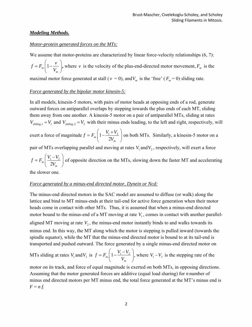
Motor-protein generated forces on the MTs:
We assume that motor-proteins are characterized by linear force-velocity relationships (6, 7):
1mm
vf F
V
, where v is the velocity of the plus-end-directed motor movement, mF is the
maximal motor force generated at stall ( v = 0), and mV is the ‘free’ ( mF = 0) sliding rate.
Force generated by the bipolar motor kinesin-5:
In all models, kinesin-5 motors, with pairs of motor heads at opposing ends of a rod, generate outward forces on antiparallel overlaps by stepping towards the plus ends of each MT, sliding them away from one another. A kinesin-5 motor on a pair of antiparallel MTs, sliding at rates
,1 1slidingV V and ,2 2slidingV V with their minus ends leading, to the left and right, respectively, will
exert a force of magnitude 1 212m
m
V Vf F
V
on both MTs. Similarly, a kinesin-5 motor on a
pair of MTs overlapping parallel and moving at rates 1V and 2V , respectively, will exert a force
1 2
2mm
V Vf F
V
of opposite direction on the MTs, slowing down the faster MT and accelerating
the slower one.
Force generated by a minus-end directed motor, Dynein or Ncd:
The minus-end directed motors in the SAC model are assumed to diffuse (or walk) along the lattice and bind to MT minus-ends at their tail-end for active force generation when their motor heads come in contact with other MTs. Thus, it is assumed that when a minus-end directed
motor bound to the minus-end of a MT moving at rate 1V , comes in contact with another parallel-
aligned MT moving at rate 2V , the minus-end motor instantly binds to and walks towards its
minus end. In this way, the MT along which the motor is stepping is pulled inward (towards the spindle equator), while the MT that the minus-end directed motor is bound to at its tail-end is transported and pushed outward. The force generated by a single minus-end directed motor on
MTs sliding at rates 1V and 2V is 1 21mm
V Vf F
V
, where 1 2V V is the stepping rate of the
motor on its track, and force of equal magnitude is exerted on both MTs, in opposing directions. Assuming that the motor generated forces are additive (equal load sharing) for n number of minus end directed motors per MT minus end, the total force generated at the MT’s minus end is F = n f.

Brust‐Mascher, Civelekoglu‐Scholey, and Scholey Sliding Filaments in Mitosis.
3
Consequently, the minus end directed motor pulls the MTs whose minus-ends are farthest from the spindle equator inward because: (i) they mostly serve as tracks for motors bound to the minus-ends of other MTs, and (ii) the motors bound to their own minus-ends are unlikely to overlap with adjacent MTs, to walk along and to be transported and pushed outward. In contrast with that, the minus end directed motor pushes the MTs whose minus ends are near the equator outward because: (i) motors bound to their minus-ends are likely to find adjacent MT tracks to move along, to be transported and pushed outward, and (ii) there are fewer MT minus-ends near the equator, hence fewer minus-end directed motors to use them as tracks to walk along and pull them inward. This mechanism thus leads to a cooperative action of kinesin-5 and minus-end directed motors near the equator, but this cooperation is progressively lost towards regions away from the equator, and where motors balance one another, MTs’ minus-ends remain immobile, forming the spindle poles.
Computational Framework and Numerical Methods:
In this section, we will describe the computational model framework, numerical methods and the algorithm used for solving the FB equations.
Computational FB Model and Numerical Solutions:
Our computational force-balance model describes a system of dynamic MTs and motors (bipolar kinesins, minus-end directed motors, and kinesin-13 depolymerases) acting on parallel and antiparallel MT overlaps and/or MT minus ends to generate forces on the MTs and the spindle poles or to depolymerize MT minus ends. In the computational model MTs are nucleated from seeds spread throughout the spindle. A pre-determined and equal number of MT nucleation seeds are allowed in each half spindle (typically 300-1000) and MTs grow towards the spindle equator from these seeds to form transient parallel and/or antiparallel overlaps. The minus end directed motors are assumed to bind instantly to newly nucleated MT minus ends at their tail end. The bipolar motors are assumed to instantly bind to dynamic MT overlaps (parallel and antiparallel) as they form. As a result of the forces generated by multiple motors MTs slide inwards or outwards. All MTs undergo MT dynamic instability (DI) at their plus ends and, when applicable, depolymerize at their pole associated minus ends as a result of the action of kinesin-13 depolymerases. In our computational model, at every time step, we keep track of each MT’s plus and minus end positions and the positions of the spindle poles. All random events described below are implemented by using the built-in uniform random number generating function rand in MATLAB™, unless otherwise specified.
Initial conditions. In our models, at the initial time step (t=0) typically 600 MTs of random
lengths ranging between 0.5 and 4 m are positioned randomly, with their minus ends at most 2 -
5 m away from the spindle equator (i.e. the spindle is initially at most 4-10 m long). The position of the spindle poles is defined as the farthest position of the MT minus ends in each half spindle region. An initial dynamic randomly state is assigned to each MT plus end.

Brust‐Mascher, Civelekoglu‐Scholey, and Scholey Sliding Filaments in Mitosis.
4
MT plus end dynamics. As previously described (8, 9) the dynamics of MT plus ends is computed in a Monte Carlo approach. At any given time, the MTs are either in a growth or a shrinkage state and their dynamics is fully described by the four parameters of dynamic instability: vg, vs, fcat, and fres. The growth/polymerization and shrinkage/depolymerization rates are fixed. The catastrophe and rescue frequencies are generally fixed, but one or both are re-assigned new fixed or spatially dependent values for the transition to spindle elongation. At each time step, first the new dynamic state of each MT is computed: for each MT plus end undergoing growth (or shrinkage) in the previous time step, a catastrophe (or rescue) event occurs if a
random number r satisfies r < Pcat(x) = 1- exp(-fcat t) (or if r < Pres = 1- exp(-fres t)) where t is the simulation time step. Once the state of each MT tip is determined in the current time step, the growth/shrinkage events of MT tips is executed and their new positions are computed. In addition, if a MT plus tip reaches the opposing pole it switches to shrinkage. If a MT shrinks to its seed, a new randomly chosen seed position is assigned in the same half spindle. In the “Slide and Cluster” model, the new random seed position is biased towards the spindle equator. This is implemented by a step change in the nucleation rate at a fixed distance away from the spindle
equator (typically nucldistance = 2 m), and a fixed step increase in nucleation rate across this position (typically nuclfold = 3), higher near the spindle equator. For each such event, two random numbers are selected: r1 and r2. If r1 < 1/( nuclfold +1), then the seed position is outside the low nucleation region (between the spindle pole and up to nucldistance to the spindle equator)
otherwise it is within the high nucleation region (within nucldistance m around the spindle equator, in the appropriate spindle half). The second random number, r2, is used to determine the random position of the seed within the assigned low/high nucleation region of the spindle (e.g. in the left half spindle, LowNucleationRegion = [ leftpole, equator- nucldistance ] and HighNucleationRegion = [equator- nucldistance, equator] ).
MT minus end dynamics. As previously described (8) in the SAFE model and the Combined model, MT minus ends that come into contact with the spindle poles are depolymerized at rate vdepoly during preanaphase, restricting the exertion of force on the spindle poles by outward sliding MTs.
Algorithm. At each time step, first the current parallel and antiparallel MT overlaps are computed and the number of motors on each overlap is updated based on the number of motors per parallel, anti-parallel unit overlap length (kp and kap, respectively), and the actual length of overlap, and stored. Then, the large coupled set of FB and kinematic equations for all MT mini-bundles, as described above, is set up using the current number of motors and MT overlaps, and solved. The solution to these equations yields the instantaneous velocity of all parallel and antiparallel overlapping MTs (Vi(t)) and the left and right spindle poles (VL(t) and VR(t)) based on the force exerted on each MT and on the spindle poles. Next, assuming that non-overlapping ‘free’ MTs in the spindle move at the average rate of MTs in their vicinity, the spindle is partitioned into four equal length quarters between the poles, and an instantaneous (current time step) average velocity of MTs in each spindle quarter is computed as the mean velocity of all the parallel and

Brust‐Mascher, Civelekoglu‐Scholey, and Scholey Sliding Filaments in Mitosis.
5
antiparallel overlapping MTs whose mid-points are within the quarter in question. Then, the instantaneous velocity of MTs that do not overlap with any other adjacent MT are assigned and stored as the average MT velocity associated with the spindle quarter their mid-point is located at. Next, the time step is incremented and the minus and plus end positions of all MTs, and the positions of the spindle poles are updated using the computed velocities. Subsequently, the dynamic states and growth/shrinkage rates of the MT plus ends are computed using the updated positions of the MTs, and based on the kinetic -rates and states of each MT plus end, and the dynamics is executed by repositioning the MT plus ends according to the event and rate of each MT plus end. If the MT minus ends are assumed to undergo depolymerization in the model considered, the new positions of MT minus ends due to depolymerization at the spindle poles are computed and updated. In the new time step, with the new positions of MTs’ plus and minus ends, the new parallel and antiparallel overlaps are computed and the sequence of steps described above is repeated.
All models are solved using custom made MATLAB™ codes, run on a personal laptop computer.
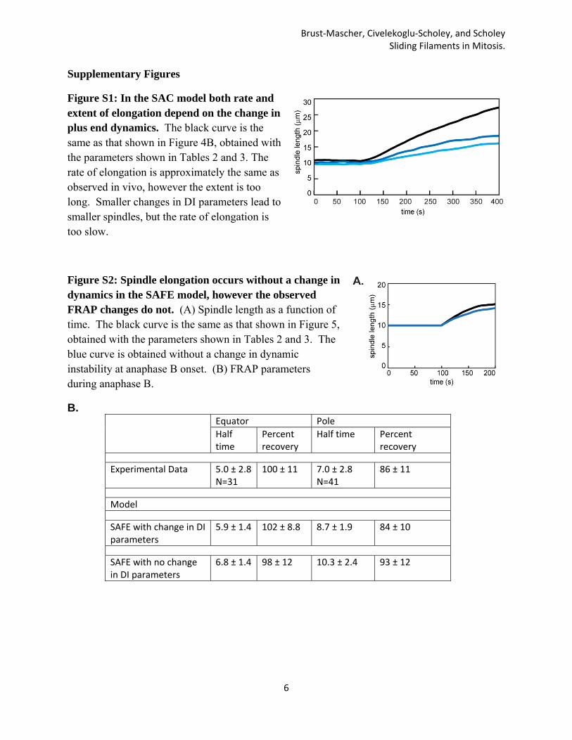
Brust‐Mascher, Civelekoglu‐Scholey, and Scholey Sliding Filaments in Mitosis.
6
Supplementary Figures
Figure S1: In the SAC model both rate and extent of elongation depend on the change in plus end dynamics. The black curve is the same as that shown in Figure 4B, obtained with the parameters shown in Tables 2 and 3. The rate of elongation is approximately the same as observed in vivo, however the extent is too long. Smaller changes in DI parameters lead to smaller spindles, but the rate of elongation is too slow.
Figure S2: Spindle elongation occurs without a change in dynamics in the SAFE model, however the observed FRAP changes do not. (A) Spindle length as a function of time. The black curve is the same as that shown in Figure 5, obtained with the parameters shown in Tables 2 and 3. The blue curve is obtained without a change in dynamic instability at anaphase B onset. (B) FRAP parameters during anaphase B.
B. Equator Pole
Half time
Percent recovery
Half time Percent recovery
Experimental Data 5.0 ± 2.8N=31
100 ± 11 7.0 ± 2.8 N=41
86 ± 11
Model
SAFE with change in DI parameters
5.9 ± 1.4 102 ± 8.8 8.7 ± 1.9 84 ± 10
SAFE with no change in DI parameters
6.8 ± 1.4 98 ± 12 10.3 ± 2.4 93 ± 12

Brust‐Mascher, Civelekoglu‐Scholey, and Scholey Sliding Filaments in Mitosis.
7
Figure S3: Effect of changes in the bipolar motor parameters on spindle length for the SAC (left) and SAFE (right) models. In all cases the blue curve is the curve obtained with the parameters in Tables 2 and 3 and shown in Figures 4B and 5. Parameters were decreased (red curve) or increased (green curve) to the values shown in the legends. In both models spindle length is sensitive to the maximal velocity.

Brust‐Mascher, Civelekoglu‐Scholey, and Scholey Sliding Filaments in Mitosis.
8
Figure S4: The spindle length in the SAC model is relatively insensitive to changes in the minus end directed motor parameters. In all cases the blue curve is the curve obtained with the parameters in Tables 2 and 3 and shown in Figure 4B. Parameters were decreased (red curve) or increased (green curve) to the values shown in the legends.

Brust‐Mascher, Civelekoglu‐Scholey, and Scholey Sliding Filaments in Mitosis.
9
Supporting References
1. Brust‐Mascher, I., G. Civelekoglu‐Scholey, and J. M. Scholey. 2014. Analysis of mitotic protein dynamics and function in Drosophila embryos by live cell imaging and quantitative modeling. Methods Mol Biol 1136:3‐30.
2. Sharp, D. J., K. L. McDonald, H. M. Brown, H. J. Matthies, C. Walczak, R. D. Vale, T. J. Mitchison, and J. M. Scholey. 1999. The bipolar kinesin, KLP61F, cross‐links microtubules within interpolar microtubule bundles of Drosophila embryonic mitotic spindles. J Cell Biol 144:125‐138.
3. Wang, H., I. Brust‐Mascher, G. Civelekoglu‐Scholey, and J. M. Scholey. 2013. Patronin mediates a switch from kinesin‐13‐dependent poleward flux to anaphase B spindle elongation. J Cell Biol 203:35‐46.
4. Lele, T. P., and D. E. Ingber. 2006. A mathematical model to determine molecular kinetic rate constants under non‐steady state conditions using fluorescence recovery after photobleaching (FRAP). Biophys Chem 120:32‐35.
5. Phair, R. D., and T. Misteli. 2000. High mobility of proteins in the mammalian cell nucleus. Nature 404:604‐609.
6. Valentine, M. T., P. M. Fordyce, T. C. Krzysiak, S. P. Gilbert, and S. M. Block. 2006. Individual dimers of the mitotic kinesin motor Eg5 step processively and support substantial loads in vitro. Nat Cell Biol 8:470‐476.
7. Toba, S., T. M. Watanabe, L. Yamaguchi‐Okimoto, Y. Y. Toyoshima, and H. Higuchi. 2006. Overlapping hand‐over‐hand mechanism of single molecular motility of cytoplasmic dynein. Proc Natl Acad Sci U S A 103:5741‐5745.
8. Brust‐Mascher, I., G. Civelekoglu‐Scholey, M. Kwon, A. Mogilner, and J. M. Scholey. 2004. Model for anaphase B: role of three mitotic motors in a switch from poleward flux to spindle elongation. Proc Natl Acad Sci U S A 101:15938‐15943.
9. Cheerambathur, D. K., G. Civelekoglu‐Scholey, I. Brust‐Mascher, P. Sommi, A. Mogilner, and J. M. Scholey. 2007. Quantitative analysis of an anaphase B switch: predicted role for a microtubule catastrophe gradient. J Cell Biol 177:995‐1004.