mech 510 computational methods in transport phenomena itetra.mech.ubc.ca/mech510/handouts.pdf ·...

Mech 510Computational Methods in Transport

Phenomena I

Carl Ollivier-Gooch

UBC Department of Mechanical Engineering

Contents

1 Intro to CFD 1

1.1 Modeling . . . . . . . . . . . . . . . . . . . . . . . . . . . . . . . 1

1.2 Discretization . . . . . . . . . . . . . . . . . . . . . . . . . . . . . 4

1.3 Accuracy and Stability . . . . . . . . . . . . . . . . . . . . . . . . 5

1.4 Validation . . . . . . . . . . . . . . . . . . . . . . . . . . . . . . . 6

1.5 Efficiency . . . . . . . . . . . . . . . . . . . . . . . . . . . . . . . 8

1.6 Convergence . . . . . . . . . . . . . . . . . . . . . . . . . . . . . 8

2 Modeling Based on the Navier-Stokes Equations 9

2.1 Non-dimensionalization of the Navier-Stokes equations . . . . . . . 9

2.2 Derivation of model problems . . . . . . . . . . . . . . . . . . . . 13

3 Space Discretization of PDE’s 15

3.1 Overview . . . . . . . . . . . . . . . . . . . . . . . . . . . . . . . 15

3.2 Transformation of a PDE into Control Volume Form . . . . . . .. 22

3.3 Second-order Accurate Flux for the Poisson Equation . . .. . . . . 23

3.4 Flux Integrals . . . . . . . . . . . . . . . . . . . . . . . . . . . . . 26

3.5 Problems . . . . . . . . . . . . . . . . . . . . . . . . . . . . . . . 27

4 Accuracy Assessment for Numerical Solutions 29

4.1 If an exact solution is available . . . . . . . . . . . . . . . . . . . .29

4.2 If an exact solution isnot available . . . . . . . . . . . . . . . . . . 30

4.3 Problems . . . . . . . . . . . . . . . . . . . . . . . . . . . . . . . 31

i

ii CONTENTS

5 Time Accuracy and Stability Analysis for Ordinary Differe ntial Equa-tions 33

5.1 From PDE to Coupled ODE’s . . . . . . . . . . . . . . . . . . . . . 33

5.2 Analysis of Time March Schemes for ODE’s . . . . . . . . . . . . 35

5.3 Caveats . . . . . . . . . . . . . . . . . . . . . . . . . . . . . . . . 37

5.4 Examples . . . . . . . . . . . . . . . . . . . . . . . . . . . . . . . 37

5.5 Stability Analysis for Fully-Discrete Systems . . . . . . .. . . . . 43

5.6 Examples . . . . . . . . . . . . . . . . . . . . . . . . . . . . . . . 44

5.7 Problems . . . . . . . . . . . . . . . . . . . . . . . . . . . . . . . 45

6 Systems of PDE’s 47

6.1 Computation of Flux and Source Jacobians . . . . . . . . . . . . .49

6.2 Problems . . . . . . . . . . . . . . . . . . . . . . . . . . . . . . . 52

7 Practical Aspects of Solving Poisson’s Equation 55

7.1 Solving the Discrete Poisson Equation . . . . . . . . . . . . . . .. 55

7.2 Boundary Conditions for the Laplacian . . . . . . . . . . . . . . .. 60

8 The Wave Equation 65

8.1 Boundary Conditions for the Wave Equation . . . . . . . . . . . .. 66

8.2 Basic Results for the Wave Equation . . . . . . . . . . . . . . . . . 67

8.3 Advanced Schemes for the Wave Equation . . . . . . . . . . . . . . 70

9 The Incompressible Energy Equation 83

9.1 Simple Discretization of the Incompressible Energy Equation . . . . 85

9.2 Time Discretization of the Energy Equation . . . . . . . . . . .. . 86

9.3 Approximate Factorization . . . . . . . . . . . . . . . . . . . . . . 90

9.4 Boundary Conditions . . . . . . . . . . . . . . . . . . . . . . . . . 91

9.5 Outline of Navier-Stokes Code . . . . . . . . . . . . . . . . . . . . 95

CONTENTS iii

A Glossary 97

B Some Mathematical Concepts Useful for CFD 101

B.1 Classification of PDE’s . . . . . . . . . . . . . . . . . . . . . . . . 101

B.2 Taylor Series Expansions . . . . . . . . . . . . . . . . . . . . . . . 101

B.3 Eigenvalues, Eigenvectors, and All That . . . . . . . . . . . . .. . 102

C Solution of Tri-Diagonal Systems of Equations 105

C.1 The Thomas Algorithm . . . . . . . . . . . . . . . . . . . . . . . . 105

C.2 The Thomas Algorithm for Systems . . . . . . . . . . . . . . . . . 106

D Programming Guidelines 109

D.1 Sample Program in C . . . . . . . . . . . . . . . . . . . . . . . . . 110

D.2 Sample Program in Fortran . . . . . . . . . . . . . . . . . . . . . . 113

D.3 Painless Array Manipulation . . . . . . . . . . . . . . . . . . . . . 116

D.4 Most Popular CFD Programming Errors . . . . . . . . . . . . . . . 120

E Validating CFD Programs 121

E.1 Modeling . . . . . . . . . . . . . . . . . . . . . . . . . . . . . . . 122

E.2 Validation . . . . . . . . . . . . . . . . . . . . . . . . . . . . . . . 123

F References 125

iv CONTENTS

List of Figures

1.1 Schematic representation of finite difference approximation to acontinuous solution. . . . . . . . . . . . . . . . . . . . . . . . . . . 4

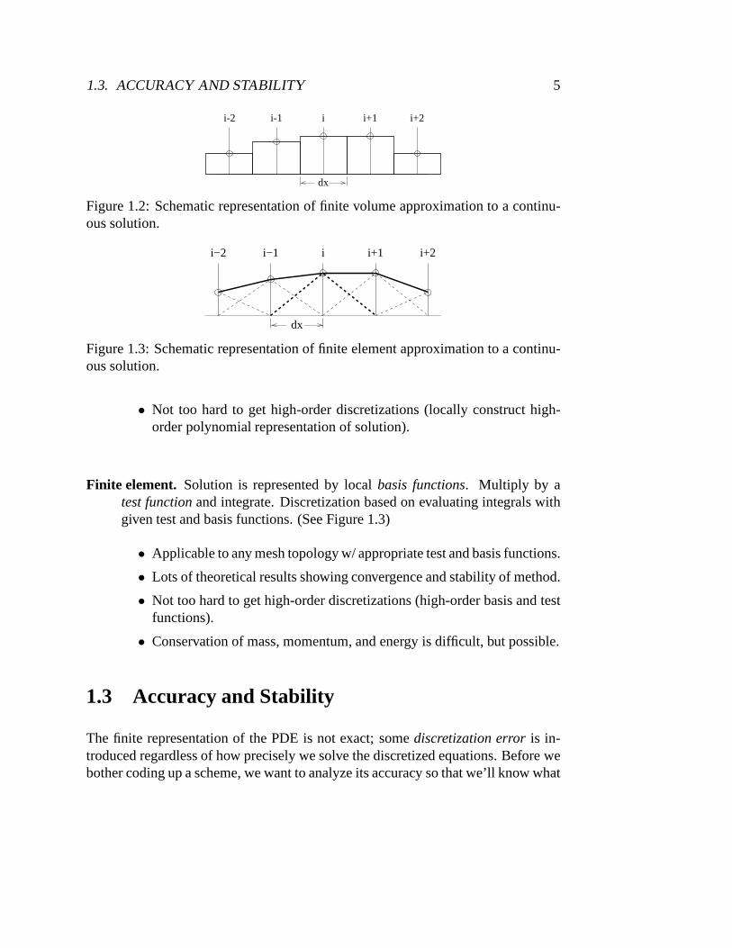
1.2 Schematic representation of finite volume approximation to a con-tinuous solution. . . . . . . . . . . . . . . . . . . . . . . . . . . . . 5

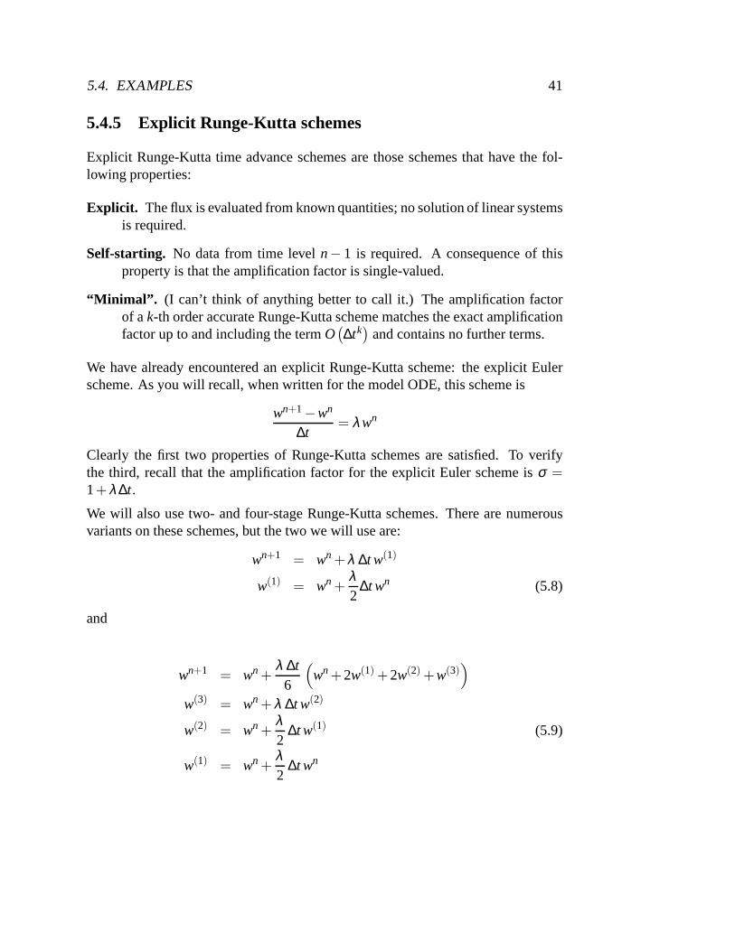
1.3 Schematic representation of finite element approximation to a con-tinuous solution. . . . . . . . . . . . . . . . . . . . . . . . . . . . . 5

3.1 Flux integration around a finite volume. . . . . . . . . . . . . . .. 26

7.1 Comparison of convergence rates for point iterative schemes ap-plied to Laplace’s equation. . . . . . . . . . . . . . . . . . . . . . . 59

7.2 Comparison of convergence rates for point and line Gauss-Seideliterative schemes applied to Laplace’s equation. . . . . . . . .. . . 60

7.3 Finite volume with homogeneous Neumann boundary condition im-posed along once side. . . . . . . . . . . . . . . . . . . . . . . . . 61

7.4 Boundary cell showing Dirichlet boundary condition andghost cell. 62

8.1 First-order time advance for the wave equation with several spacediscretizations . . . . . . . . . . . . . . . . . . . . . . . . . . . . . 68

8.2 Second-order time advance for the wave equation with several spacediscretizations . . . . . . . . . . . . . . . . . . . . . . . . . . . . . 69

8.3 Second-order time advance for the wave equation propagating asquare wave. . . . . . . . . . . . . . . . . . . . . . . . . . . . . . . 69

8.4 Effect of mesh refinement on square wave propagation using thesecond-order upwind scheme. . . . . . . . . . . . . . . . . . . . . 70

v

vi LIST OF FIGURES

8.5 Example control-volume averaged solution . . . . . . . . . . .. . 71

8.6 Legal values ofψ(r) for TVD schemes . . . . . . . . . . . . . . . . 72

8.7 Three TVD limiters . . . . . . . . . . . . . . . . . . . . . . . . . . 74

8.8 Upwind TVD schemes (square wave) . . . . . . . . . . . . . . . . 79

8.9 ENO and FCT schemes (square wave) . . . . . . . . . . . . . . . . 80

8.10 Propagation of a smooth solution (sine wave) . . . . . . . . .. . . 81

Chapter 1

Intro to CFD

Strengths of Computational/Experimental/Analytic FluidDynamics

1.1 Modeling

Consider the flow inside a commercial tire incinerator (picture shown in class).Ground-up tires are dumped in and burned. Gases pass by several heat exchang-ers to boil and superheat water for power generation. Because of the combustionconditions, there is a significant amount of nitrogen oxides(NOx) in the flue gases,which is environmentally unacceptable. A company in Illinois (Nalco Fueltech)makes a living by sellingNOx reduction systems for incinerators like this one. Theyneed an accurate CFD model that can be easily applied to a variety of incineratorsrather quickly so that they can designNOx reduction systems. In particular, theymust predict temperature, velocity, andNOx concentration both with and withouttheir emission reduction system for several operating conditions. They must do thisquickly (a couple of weeks at most).

1

2 CHAPTER 1. INTRO TO CFD

Key features of the physics: Governing equations that include most of these effects:

Global continuity:

∂ρ∂ t

+∇ · (ρ~u) = Sρ

Momentum:

∂ (ρ~u)∂ t

+∇ ·(

ρ~u⊗~u+P~I −~τi j

)

= Smom

Energy:

∂E∂ t

+∇ · (~u(E+P)) =∂Q∂ t

+∇ · (k∇T)+qrad+∇ · (~τi j ·~u)

Species continuity:

∂ρi

∂ t+∇ · (ρi~u) = Sρi

Turbulence closure model

Droplet transport and evaporation model.

Total: Perhaps twenty PDE’s with a wide range of time scales (from very fast chem-ical reactions to viscous diffusion and convection scales).

Including all of this physical detail in a computer model would make for a tremen-dously complicated and probably tremendously slow program. The essence of mod-eling is to balance physical fidelity against human and computer resources available.

1.1. MODELING 3

Generally, we use either the simplest model that gives a reasonable answer or themost complex model that can be programmed and run with available resources.

Assume for this problem that:

• Combustion can be modeled as a distributed heat source

• Sprays have a negligible mass, momentum, and energy effect on the flow

• Chemistry ofNOx reduction can be de-coupled (solved separately,a posteri-ori)

• Neglect radiative heat transfer

This reduces the mathematical description of the problem to:

Global continuity:

∂ρ∂ t

+∇ · (ρ~u) = 0

Momentum:

∂ (ρ~u)∂ t

+∇ ·(

ρ~u⊗~u+P~I −~τi j

)

= 0

Energy:

∂E∂ t

+∇ · (~u(E+P)) = ∇ · (k∇T)+∇ · (~τi j ·~u)+∂Q∂ t

Species continuity:

Removed from main model

Turbulence closure model

Droplet transport and evaporation model.

Chemical reactions in theNOx reduction process.

Total: Seven PDE’s (with 2-eq turbulence model) plus a de-coupled set of PDE’sto be solved separately for the droplets, etc, once velocities and temperatures areknown.

Modelingis the process of separating important from unimportant physical effectsin the physics of the problem to arrive at a mathematical model that is not toocomplex.


1.2 Discretization

Modeling gives a system of PDE’s to be solved. Only very rarely can we obtainan exact solution to these PDE’s. Before we can compute a solution, we first mustdecidewherewe want to solve the equations. This requires us to generate ameshcontaining a finite number of locations where we will solve the PDE’s. Mesh gen-eration is a topic that we will discuss in Mech 511.

Once we have a mesh, we need to develop a representation of thePDE’s on thismesh, including a time-evolution scheme. There are three main families of tech-niques for this:

Finite difference. Solution is represented by point values at mesh points. Replaceeach differential term in the PDE by a corresponding finite difference approx-imation. (See Figure 1.1)

i i+1 i+2i-1i-2

dx

Figure 1.1: Schematic representation of finite difference approximation to a contin-uous solution.

• The original approach for CFD.

• Easy to get high-order discretizations (use high-order finite differences).

• Doesn’t conserve mass, momentum, and energy exactly.

• Impractical for unstructured meshes.

Finite volume. Solution is represented by control volume averages. Write thePDE’s in volume integral form. Discretization based on evaluation of vol-ume integral over small control volumes. (See Figure 1.2)

• Conserves mass, momentum, and energy exactly.

• Applicable to any mesh topology w/ appropriate control volumes.

1.3. ACCURACY AND STABILITY 5

dx

i i+1 i+2i-1i-2

Figure 1.2: Schematic representation of finite volume approximation to a continu-ous solution.

i i+1 i+2i−1i−2

dx

Figure 1.3: Schematic representation of finite element approximation to a continu-ous solution.

• Not too hard to get high-order discretizations (locally construct high-order polynomial representation of solution).

Finite element. Solution is represented by localbasis functions. Multiply by atest functionand integrate. Discretization based on evaluating integrals withgiven test and basis functions. (See Figure 1.3)

• Applicable to any mesh topology w/ appropriate test and basis functions.

• Lots of theoretical results showing convergence and stability of method.

• Not too hard to get high-order discretizations (high-orderbasis and testfunctions).

• Conservation of mass, momentum, and energy is difficult, butpossible.

1.3 Accuracy and Stability

The finite representation of the PDE is not exact; somediscretization erroris in-troduced regardless of how precisely we solve the discretized equations. Before webother coding up a scheme, we want to analyze its accuracy so that we’ll know what


we’re getting. The analysis gives an idea about how much difference there will bebetween our discrete solution (on a computer with infinite precision) and the exactsolution to the PDE. We also find out how the discretization error will change as weadd mesh points.

Also, for unsteady problems, we analyze the time-evolutionscheme to determineits stability. That is, we determine whether errors in the solution will grow expo-nentially in time or remain bounded.

1.4 Validation

Then we write a program to solve the discrete problem. We compile it. It doesn’tcompile the first few times. Finally it does. We run it. It crashes. Finally it runs andgives an answer. Should we believe this answer? No. Absolutely not. The outputcould be literally anything, from Egyptian hieroglyphics to the Martian alphabet;these are about as likely as getting the right solution the first try, in my experience.No CFD program should be considered correct until it has beenthoroughly testedand debugged.

There are two interrelated parts to fixing a broken CFD program. Validation tellsus whether the solutions we get for a series of simple test cases are correct.Debug-ging is the process of identifyingwhya program failed a test case and fixing it. Avalidation plan should begin with ridiculously simple testcases and work up to testcases that are as near as possible in complexity to the problem to be solved.

• Begin by testing code at the component level. While it’s possible to debug1000 lines of code (about the limit of program size for this course, typically)in one big piece, it’s much easier to work with much smaller chunks. Basi-cally, if you can define a task that a chunk of code is supposed to do, you candefine a test that confirms that it was done correctly. Writingthe testfirst isnot necessarily a bad idea — then you’ll know for sure when you’re done.

• When testing the entire code by solving flow problems,

– Each test case should have a known solution, whether analytic, experi-mental, or computed by a previously-validated program.

– Each test case should ideally test a single new part of the physics or asingle new interaction between already validated parts. This approach

1.4. VALIDATION 7

minimizes the number of places one must look for errors when the pro-gram gives an incorrect result for a test case; this more thanoffsets thetime consumed in running more test cases. While it is nearly impossi-ble to test only one thing with each case, the closer we come todevisingsuch a plan, the easier it will be to validate and debug our program.

– Table 1.1 gives a partial listing of test problems worth considering forthe tire incinerator problem.

Case Physics Change inphysics

1 Inviscid terms only, no heat addition, no flow ini-tial condition in a closed rectangular box (ana-lytic solution)

2 Inviscid terms only, no heat addition, no flowinitial condition with wall, inflow, and outflowboundary conditions (analytic solution)

Differentboundaryconditions

3 Inviscid terms only, no heat addition, uniformflow in a straight rectangular duct (analytic so-lution)

Non-zerovelocity

4 Inviscid terms only, no heat addition, accelerat-ing flow in a straight rectangular duct (analyticsolution)

Velocity in-creasing tosteady-state

n-3 Turbulent flow without heat addition in a straightduct (experimental data)

Turbulence

n-2 Turbulent flow with heat addition in a straightduct (experimental data)

Heat addition

n-1 Turbulent flow without heat addition in a ductwith abrupt turns (experimental data)

Flow aroundbends

n Turbulent flow with heat addition in tire inciner-ator

Combines n-2and n-1

Table 1.1: Partial validation plan for the tire incineratorproblem.

Technically, the listing of test cases for the tire incinerator problem mixes validationcases and verification cases. The difference between these two categories is that


verificationensures that your program correctly implements the physicsthat youintended it to, whilevalidationdemonstrates that your physical model comes closeenough to reality for the problem of interest.

1.5 Efficiency

Now the program works, and we believe that the physics it simulates is adequatefor our real world problem. Is the code efficient enough to be usable? Let’s say thata run for this tire incinerator takes 20 CPU hours on the fastest machine available.For one run, that would be fine. But in the design context, we have to check anumber of different operating conditions, which starts to get expensive. And for thecompany to stay in business, we have to design an emission reduction system forone of these things every week or so. So in this case, 20 hours isn’t good enough.We have to go back and do one of several things:

• Simplify the physical model even more

• Simplify the discretization

• Improve the technique we use to solve the discretized equations

• Buy a faster computer

Whatever we do, we have to sure that the final solution is stillaccurate enough.

1.6 Convergence

Finally, for any problem, we need to be sure that we have adequately resolved allof the important physical features of the flow. “Important” depends on the physicalquantities we’re after. If all we care about isNOx mass fraction at the stack outflow,then we probably do not need to be concerned with resolving the length scalesof turbulent eddies. To know this, we need either enough experience to know inadvance how fine a mesh to use or to perform amesh refinement study. In a meshrefinement study, we compute the solution on a series of progressively finer meshesuntil the physical quantity in which we are interested stopschanging. This amountsto an empirical measurement of when discretization error isacceptably small.

Chapter 2

Modeling Based on the Navier-StokesEquations

Most problems in computational fluid dynamics and computational heat transferhinge on solving the Navier-Stokes equations, which describe viscous fluid flow,often in conjunction with auxiliary equations describing other physical phenomena,like turbulence, combustion, transport of chemical species, etc. Before consideringsuch complicated cases, we will begin by examining the Navier-Stokes equationsin detail, including non-dimensionalizing the basic equations and deriving somesimple model problems based on that non-dimensional form.

2.1 Non-dimensionalization of the Navier-Stokes equa-tions

First, we write the Navier-Stokes equations (including theenergy equation) in twodimensions for the case of constant coefficients:

∂u∂x

+∂v∂y

= 0 (2.1)

∂u∂ t

+∂u2

∂x+

∂uv∂y

= −1ρ

∂P∂x

+ν(

∂ 2u∂x2 +

∂ 2u∂y2

)

(2.2)

∂v∂ t

+∂uv∂x

+∂v2

∂y= −1

ρ∂P∂y

+ν(

∂ 2v∂x2 +

∂ 2v∂y2

)

(2.3)

9

10CHAPTER 2. MODELING BASED ON THE NAVIER-STOKES EQUATIONS

∂T∂ t

+u∂T∂x

+v∂T∂y

=k

ρcp

(

∂ 2T∂x2 +

∂ 2T∂y2

)

(2.4)

+νcp

(

2

(

∂u∂x

)2

+2

(

∂v∂y

)2

+

(

∂v∂x

+∂u∂y

)2)

Note that the momentum equations have been written in conservation-law formby using the continuity equation. The same thing could have been done for theenergy equation, but this equation is generally solved separately, with the velocityfield already known; this makes it much less important to havethis equation inconservation law form.

To non-dimensionalize Equations 2.1–2.4, we need reference values for length, ve-locity, pressure, and temperature (density is fixed, so we don’t need a referencevalue for density). Suppose that we choose to non-dimensionalize length byL,velocity byuref, pressure byρu2

ref, and temperature byTref. Basically, we just as-sume that we can find some appropriate reference valuesL, uref andTref for what-ever problem we’re solving and that the pressure changes in the flow can be non-dimensionalized appropriately by the dynamic pressure associated withuref. If wedo this, we can write the dimensional variables in terms of non-dimensional vari-ables (with∗) and reference values:

t = t∗L

uref

x = x∗L

y = y∗L

u = u∗uref

v = v∗uref

P = P∗ρu2ref

T = T∗Tref

Substituting these into the continuity equation:

∂ (u∗uref)

∂ (x∗L)+

∂ (v∗uref)

∂ (x∗L)= 0

oruref

L

(

∂u∗

∂x∗+

∂v∗

∂y∗

)

= 0

or∂u∗

∂x∗+

∂v∗

∂y∗= 0

2.1. NON-DIMENSIONALIZATION OF THE NAVIER-STOKES EQUATIONS11

Substituting into the x-momentum equation:

∂ (u∗uref)

∂ (t∗L/uref)+

∂(

u∗2u2

ref

)

∂ (x∗L)+

∂(

u∗v∗u2ref

)

∂ (y∗L)=−1

ρ∂(

P∗ρu2ref

)

∂ (x∗L)+ν

(

∂ 2(u∗uref)

∂(

x∗2L2) +

∂ 2(u∗uref)

∂(

y∗2L2)

)

Dividing all terms byu2ref/L,

∂u∗

∂ t∗+

∂u∗2

∂x∗+

∂u∗v∗

∂y∗=−∂P∗

∂x∗+

νLuref

(

∂ 2u∗

∂x∗2+

∂ 2u∗

∂y∗2

)

where of course νLuref≡ 1

Re. Not surprisingly, a similar result holds for the y-momentum equation:

∂v∗

∂ t∗+

∂u∗v∗

∂x∗+

∂v∗2

∂y∗=−∂P∗

∂y∗+

νLuref

(

∂ 2v∗

∂x∗2+

∂ 2v∗

∂y∗2

)

If we substitute the non-dimensional versions of the variables into the energy equa-tion, we get:

∂ (T∗Tref)

∂ (t∗L/uref)+u∗uref

∂ (T∗Tref)

∂ (x∗L)+v∗uref

∂ (T∗Tref)

∂ (y∗L)=

kρcp

Tref

L2

(

∂ 2T∗

∂x∗2+

∂ 2T∗

∂y∗2

)

+νcp

u2ref

L2

(

2

(

∂u∗

∂x∗

)2

+2

(

∂v∗

∂y∗

)2

+

(

∂v∗

∂x∗+

∂u∗

∂y∗

)2)

Dividing by urefTref/L, we get:

∂T∗

∂ t∗+u∗

∂T∗

∂x∗+v∗

∂T∗

∂y∗=

kρcpLuref

(

∂ 2T∗

∂x∗2+

∂ 2T∗

∂y∗2

)

+νuref

cpTrefL

(

2

(

∂u∗

∂x∗

)2

+2

(

∂v∗

∂y∗

)2

+

(

∂v∗

∂x∗+

∂u∗

∂y∗

)2)

What are the dimensionless parameters here?

ρLuref cp

k=

ρLuref

µµcp

k= Re·Pr=

inertiaviscosity

dissipationconduction


andcpTref L

uref ν=

Luref

νcpTref

u2ref

= Re· 1Ec

=inertia

viscosityenthalpy

kinetic energy

Summarizing the non-dimensional equations,

∂u∗

∂x∗+

∂v∗

∂y∗= 0 (2.5)

∂u∗

∂ t∗+

∂u∗2

∂x∗+

∂u∗v∗

∂y∗= −∂P∗

∂x∗+

1Re

(

∂ 2u∗

∂x∗2+

∂ 2u∗

∂y∗2

)

(2.6)

∂v∗

∂ t∗+

∂u∗v∗

∂x∗+

∂v∗2

∂y∗= −∂P∗

∂y∗+

1Re

(

∂ 2v∗

∂x∗2+

∂ 2v∗

∂y∗2

)

(2.7)

∂T∗

∂ t∗+u∗

∂T∗

∂x∗+v∗

∂T∗

∂y∗=

1Re·Pr

(

∂ 2T∗

∂x∗2+

∂ 2T∗

∂y∗2

)

(2.8)

+EcRe

(

2

(

∂u∗

∂x∗

)2

+2

(

∂v∗

∂y∗

)2

+

(

∂v∗

∂x∗+

∂u∗

∂y∗

)2)

Note the extreme similarity in form between Equations 2.1–2.4 on the one hand andEquations 2.5–2.8. From now on, we’ll use the non-dimensional form without the∗ superscripts.

Finally, it’s worth noting that the non-dimensional parameters depend only on fluidproperties (which we are assuming to be fixed) and on the reference values:

Re =ρLuref

µ=

Luref

ν

Pr =µcp

k

Ec =u2

ref

cpTref

We can deduce several things from the way in which these non-dimensional coeffi-cients appear in the non-dimensional equations.

• The viscous terms in the momentum equations will be important unless theReynolds number is extremely large, and these terms will dominate the mo-mentum equations in the limit of low Reynolds number (creeping flow). The

2.2. DERIVATION OF MODEL PROBLEMS 13

heat conduction and viscous dissipation terms in the energyequation alsohave Reynolds number scaling, with the same consequences.

• The heat conduction term has an additional dependence on thePrandtl num-ber, which is a fluid property that measures whether momentumor heat dif-fuses more rapidly in the fluid.

• The viscous dissipation has an additional dependence on theEckert number,which is a measure of the relative importance of internal energy and kineticenergy in the flow.

2.2 Derivation of model problems

Although the Navier-Stokes equations are useful for solving physical problems,there are too many complexities involved in their solution for them to be a goodstarting point for study. However, we can derive several pedagogically useful modelproblems from the Navier-Stokes equations that can be used to illustrate particulartechniques in CFD.

Poisson’s Equation

Begin with the two-dimensional incompressible energy equation, including a sourceterm:

∂T∂ t

+u∂T∂x

+v∂T∂y

=1

Re·Pr∇2T +

EcRe

(

2

(

∂u∂x

)2

+2

(

∂v∂y

)2

+

(

∂v∂x

+∂u∂y

)2)

+ Q

Assume steady-state and zero velocity:

1Re·Pr

∇2T = −Q

∂ 2T∂x2 +

∂ 2T∂y2 = −Re·PrQ≡ S

This is the familiar Poisson equation, which describes (among other things) steadyheat conduction with a heat source. This is an elliptic PDE; that is, Poisson’s equa-tion poses a pure boundary value problem, with temperature everywhere coupled totemperature everywhere else.


Heat equation

Starting again with the incompressible energy equation in two dimensions, and thistime assume zero velocity and no source term,

∂T∂ t

=1

Re·Pr

(

∂ 2T∂x2 +

∂ 2T∂y2

)

= α(

∂ 2T∂x2 +

∂ 2T∂y2

)

This is thetransient heat conduction equationor heat equation. This is a parabolicPDE, so the heat equation poses an initial-boundary value problem. The solution at(x, t) depends on the solution at allx at that time.

Wave equation

Begin yet again with the incompressible energy equation, and assume zero viscosityand thermal conductivity. Also, neglect the source term. Then we get:

∂T∂ t

+u∂T∂x

+v∂T∂y

= 0

If we know the velocity, then this is a hyperbolic PDE for the temperature T. Thisis the wave equation, which is an initial-value problem. Forone dimension, we get

∂T∂ t

+u∂T∂x

= 0

This is the linear convection equation in one dimension. This problem has a generalsolution of the form

E(x,ut) = f (x−ut)

so solutions travel unchanged at constant speed.

For what other bits of the physics of the Navier-Stokes equations is this a goodmodel? That is, what other flow quantities are carried along with the flow?

Chapter 3

Space Discretization of PDE’s

Suppose we have a general conservation law (with source term) of the form1

∂U∂ t

+∂F∂x

+∂G∂y

+∂H∂z

= S (3.1)

Before we can compute the solution of this problem, we must rewrite the PDE intoa system of algebraic equations relating the solution at onetime level to the solutionat the next time level. The first step in this process is space discretization, whichwill convert the PDE into a system of coupled ODE’s describing the variation ofsolution unknowns with time. Next, these ODE’s are discretized in time to producea set of algebraic equations.

3.1 Overview

We begin with a comparison among finite difference, finite element, and finite vol-ume methodologies. These methods can all be applied to the PDE in Eq. 3.1, butfor simplicity and concreteness, we will consider the one-dimensional advection-diffusion equation:

∂T∂ t

+∂uT∂x

= α∂ 2T∂x2

1This form is much more general than it looks. In particular, it is a simple matter to write theNavier-Stokes equations in this form.

15

16 CHAPTER 3. SPACE DISCRETIZATION OF PDE’S

whereu andα are known constants. We consider the spatial domain[0,1], dividedinto N equal intervals, withT (0, t) = 1 and ∂T

∂x (1, t) = 0. Initial conditions neednot concern us here.

3.1.1 The Finite Difference Method

In the finite difference methods, we compute the solution at points in the domain.In this case, we will haveN+1 points located atxi =

iN , i = 0..N. We will refer

to the solution atxi asTi. To approximate the spatial derivatives, we will use finitedifferences, just as in the classical definition of the derivative. Because there ismore than one way to approximate a derivative at a point, the discretization is notunique; one possibility is to use

∂T∂x

≈ Ti+1−Ti−1

2∆x∂ 2T∂x2 ≈ Ti+1−2Ti +Ti−1

∆x2

Using Taylor series expansions, it is easy to verify that these approximations areaccurate to withinO

(

∆x2)

; that is, that the difference between= and≈ for theseapproximations decreases with the square of the mesh spacing. In this case, we canwrite a discrete approximation to the PDE as:

dTi

dt+u

Ti+1−Ti−1

2∆x= α

Ti+1−2Ti +Ti−1

∆x2

again to withinO(

∆x2)

. This leaves usN−1 equations (for points 1 throughN−1)written in terms ofN+1 unknowns (T0 andTN are the other two). Fortunately, wehave two boundary conditions, which can again be written by replacing derivativeswith approximations:

T0 = 1TN−TN−1

∆x= 0

The former happens to be exact (no approximation was required), while the latterturns out to be first-order accurate.

3.1. OVERVIEW 17

3.1.2 The Finite Element Method

In the finite element method, the solution is computed at nodal values (here weuse the same points as in the finite difference example), and interpolated betweennodes by using basis functions so that a continuous representation of the solution isavailable. That is, the global solution is written as

T (x, t) =N

∑i=0

bi (x)Ti (3.2)

where thebi arebasis functions, and theTi are the nodal solution values (which varyin time, but this is suppressed for notational clarity). Basis functions are alwaysdefined to have a value of 1 at exactly one nodal point, and zeroat all others; thisensures that the interpolation matches the nodal values at the nodes. Basis functionsare also defined to havecompact support, meaning that they are uniformly zerooutside of a small region near “their” node. For our present purposes, we willconsider the piecewise-linear tent-shaped basis functiongiven by:

bi (x) =

1+ x−xi∆x xi−1≤ x≤ xi

1− x−xi∆x xi ≤ x≤ xi+1

0 elsewhere(3.3)

This basis function must be modified at the ends of the domain to be one sided, sothat the basis function does not overlap the end of the domain.

Finite volume discretization proceeds by multiplying the PDE by a test functionwi (x); we will consider the Galerkin finite element discretization, in which thetest and basis functions are identical. This weighted PDE isintegrated over thedomain, with the solution represented by Equation. 3.2. Repeating this for eachbasis function results inN+1 equations for the nodal solution values.

In this case, for an interior node, we write:

wi

N

∑j=0

(

b jdTj

dt

)

+uwi

N

∑j=0

(

Tjdbj

dx

)

= αwi

N

∑j=0

(

Tjd2b j

dx2

)

Note that, even for linear basis functions, the second derivative on the right-handside is non-zero atx = x j (where it is infinite). Also, for the given basis and testfunctions, the only non-zero terms occur forj = i−1, i, i +1, which reduces bothanalytic and computational effort enormously. Now we integrate over the domain,


which reduces to integration over the support ofwi :

∫ 1

0

[

wi

i+1

∑j=i−1

(

b jdTj

dt

)

+uwi

i+1

∑j=i−1

(

Tjdbj

dx

)

]

dx =∫ 1

0αwi

i+1

∑j=i−1

(

Tjd2b j

dx2

)

dx

∫ (i+1)∆x

(i−1)∆x

[

wi

i+1

∑j=i−1

(

b jdTj

dt

)

+uwi

i+1

∑j=i−1

(

Tjdbj

dx

)

]

dx =

∫ (i+1)∆x

(i−1)∆xαwi

i+1

∑j=i−1

(

Tjd2b j

dx2

)

dx

Let’s look at one term at a time. First, the advection term:

∫ (i+1)∆x

(i−1)∆xuwi

i+1

∑j=i−1

(

Tjdbj

dx

)

dx =

[

uwi

i+1

∑j=i−1

(

Tjb j)

](i+1)∆x

(i−1)∆x

−∫ (i+1)∆x

(i−1)∆xu

dwi

dx

i+1

∑j=i−1

(

Tjb j)

dx

Here we’ve used integration by parts, and note that the first term on the left is zerofor all i (except fori = N, a boundary case which we’ll ignore for now). In thesecond term, the derivative of the weight function is:

dwi

dx=

1∆x (i−1)∆x< x< i∆x−1∆x i∆x< x< (i +1)∆x

and the sum is the solution interpolant:

i+1

∑j=i−1

Tjb j =

Ti−1+(

x∆x− (i−1)

)

(Ti−Ti−1) (i−1)∆x< x< i∆xTi+1+

(

i +1− x∆x

)

(Ti−Ti+1) i∆x< x< (i +1)∆x

So that integral gets split into two pieces, thus:

−∫ (i+1)∆x

(i−1)∆xu

dwi

dx

i+1

∑j=i−1

(

Tjb j)

dx = −∫ i∆x

(i−1)∆xu

1∆x

(

Ti−1+( x

∆x− (i−1)

)

(Ti−Ti−1))

dx

−∫ (i+1)∆x

i∆xu

(−1∆x

)

(

Ti+1+(

i +1− x∆x

)

(Ti−Ti+1))

dx

= −[

u∆x

(

Ti−1x+

(

x2

2∆x− (i−1)x

)

(Ti−Ti−1)

)]i∆x

(i−1)∆x

−[−u

∆x

(

Ti+1x+

(

(i +1)x− x2

2∆x

)

(Ti−Ti+1)

)](i+1)∆x

i∆x

= − u∆x

[

Ti−1∆x+

(

(2i−1)∆x2

2∆x− (i−1)∆x

)

(Ti−Ti−1)

]

3.1. OVERVIEW 19

+u

∆x

[

Ti+1∆x+

(

(i +1)∆x− (2i +1)∆x2

2∆x

)

(Ti−Ti+1)

]

= u

[

−Ti−1−Ti−Ti−1

2+Ti+1+

Ti−Ti+1

2

]

= uTi+1−Ti−1

2

The second-last line contains the average values between(i, i +1) and(i, i−1) ina recognizable form; this isn’t surprising, considering weintegrated the solutiontimes a constant.

For the diffusive term, we’ll once again integrate by parts once:

∫ (i+1)∆x

(i−1)∆xαwi

i+1

∑j=i−1

(

Tjd2b j

dx2

)

dx=

˙[

αwi

i+1

∑j=i−1

(

Tjdbj

dx

)

](i+1)∆x

(i−1)∆x

−α∫ (i+1)∆x

(i−1)∆x

dwi

dx

i+1

∑j=i−1

(

Tjdbj

dx

)

dx

Again, except for boundary cases, the first term is zero for all i. The second termhas a piecewise constant integrand, with

i+1

∑j=i−1

Tjdbj

dx=

Ti−Ti−1∆x (i−1)∆x< x< i∆x

Ti+1−Ti∆x i∆x< x< (i +1)∆x

So that remaining integral becomes:

−α∫ (i+1)∆x

(i−1)∆x

dwi

dx

i+1

∑j=i−1

(

Tjdbj

dx

)

dx = −α[

1∆x

Ti−Ti−1

∆x+

(−1∆x

)

Ti+1−Ti

∆x

]

∆x

= αTi+1−2Ti +Ti−1

∆x

Okay, that’s two integrals out of three done. Now for the time-dependent term.Since the node locations and the basis and test functions areconstant, we can pullthe time derivative out of the integral to get:

∫ (i+1)∆x

(i−1)∆xwi

i+1

∑j=i−1

(

b jdTj

dt

)

dx=ddt

∫ (i+1)∆x

(i−1)∆xwi

i+1

∑j=i−1

(

b jTj)

dx

Now we substitute forwi andb j , and it’s easy to get to:

ddt

∫ (i+1)∆x

(i−1)∆xwi

i+1

∑j=i−1

(

b jTj)

dx =ddt

∫ i∆x

(i−1)∆x

( x∆x− (i−1)

)(

Ti−1+(Ti−Ti−1)( x

∆x− (i−1)

))

dx


+ddt

∫ (i+1)∆x

i∆x

(

i +1− x∆x

)(

Ti+1+(Ti−Ti+1)(

i +1− x∆x

))

d

= ∆xddt

(

Ti+1+4Ti +Ti−1

6

)

where the last line reflects not the occurrence of a miracle, but simply some tediousalgebra. Combining the results of evaluating these variousintegrals, we get thelinear Galerkin finite-element discretization for the advection diffusion equation:

∂T∂ t

+∂uT∂x

= α∂ 2T∂x2

(

16

dTi+1

dt+

23

dTi

dt+

16

dTi−1

dt

)

+uTi+1−Ti−1

2∆x= α

Ti+1−2Ti +Ti−1

∆x2

Note that we have a set of algebraic equations to solve for thetime derivatives. Forsteady-state computations, it’s customary to fold the left-hand side terms togetherto get simplydTi/dt; this is a specific example of the generallumped mass matrixtechnique. For boundary conditions, we once again apply

T0 = 1TN−TN−1

∆x= 0

although for unsteady problems, it’s convenient to differentiate these with respectto time.

3.1.3 The Finite Volume Method

The finite volume method divides the domain into control volumes. In this case,there areN control volumes, with control volumei covering the region from(i−1)∆xto i∆x. The quantity we compute in this case will be the control volume average ofthe solution, which we will refer to asTi ≡ 1

∆x

∫ i∆x(i−1)∆xT dx. We begin by integrating

the equations over a control volume:

∂T∂ t

+∂uT∂x

= α∂ 2T∂x2

∫

CV i

∂T∂ t

dx+∫

CV i

∂uT∂x

=∫

CV iα

∂ 2T∂x2 dx

3.1. OVERVIEW 21

Now we apply Gauss’s Theorem to convert the second and third integrals; in threedimensions, this is stated as:

∫

Ω∇ ·~F dV =

∮

∂Ω~F · ndA

where~F is an arbitrary vector and ˆn is an outward unit normal. Applying Gauss’stheorem in this one-dimensional context, we get:

∫

CV i

∂T∂ t

dx+∫

CV i

∂uT∂x

dx =∫

CV iα

∂ 2T∂x2 dx

∫

CV i

∂T∂ t

dx+(uT)x=i∆x− (uT)x=(i−1)∆x = α

(

(

∂T∂x

)

x=i∆x−(

∂T∂x

)

x=(i−1)∆x

)

For fixed control volumes, the derivative can be removed fromthe integral andconverted to a complete differential. The remaining quantities in the discretiza-tion represent fluxes across the control volume boundaries,and sensible choices forcomputing these fluxes is a key to success with the finite volume method. In thecase, we will write

(uT)x=i∆x = uTi + Ti+1

2(

∂T∂x

)

x=i∆x=

Ti+1− Ti

∆x

These choices, as we shall see, turn out to be second-order accurate. If we substitutethese expressions into our control volume averaged PDE, we get

∫

CV i

∂T∂ t

dx+(uT)x=i∆x− (uT)x=(i−1)∆x = α

(

(

∂T∂x

)

x=i∆x−(

∂T∂x

)

x=(i−1)∆x

)

∆xdTi

dt+u

Ti+1− Ti−1

2= α

Ti+1−2Ti + Ti−1

∆xdTi

dt+u

Ti+1− Ti−1

2∆x= α

Ti+1−2Ti + Ti−1

∆x2

Again, we get an interior scheme indistinguishable from thefinite difference andfinite element schemes for this problem. The boundary conditions, however, dif-fer. In this case, if we follow from the flux definitions, we findthat the boundary


conditions can be written as:

Tx=0 =T1+ T0

2= 1

(

∂T∂x

)

x=N∆x=

TN+1− TN

∆x= 0

This looks like it might be a step backwards (we’ve introduced two new variables,T0 andTN+1), the interior scheme contains these variables as well. Forinstance,

dT1

dt+u

T2− T0

2∆x= α

T2−2T1+ T0

∆x2

So in the end, we can choose to think of this as a problem withN+2 equations andN+2 unknowns.

3.2 Transformation of a PDE into Control VolumeForm

If we integrate Equation 3.1 over a three-dimensional control volume, we get

∫

CV

∂U∂ t

dV+

∫

CV

∂F∂x

dV+

∫

CV

∂G∂y

dV+

∫

CV

∂H∂z

dV =

∫

CVSdV

∫

CV

∂U∂ t

dV+∫

CV

(

∂F∂x

+∂G∂y

+∂H∂z

)

dV =∫

CVSdV

∫

CV

∂U∂ t

dV+

∫

CV∇ ·~F dV =

∫

CVSdV

where the last equation arises by defining~F = Fi +Gj +Hk. Using Gauss’s theo-rem, we get

∫

CV

∂U∂ t

dV+

∮

∂ (CV)~F ·~ndA=

∫

CVSdV

If we assume that the size and shape of the control volume is fixed (computationally,assume that the mesh is not moving), we can simplify a bit further.

ddt

∫

CVU dV+

∮

∂ (CV)~F ·~ndA=

∫

CVSdV (3.4)

3.3. SECOND-ORDER ACCURATE FLUX FOR THE POISSON EQUATION23

In the finite-volume method, we abandon hope of knowing anything about the de-tails of the solution within a control volume and instead content ourselves withcomputingU ≡ 1

V

∫

CVU dV. This average value isnot necessarily the value of thesolution at any fixed point within the control volume, including its centroid; for-getting this fact can lead to unfortunate misunderstandings when developing finite-volume algorithms.2

If we also define a mean source term contributionS≡ 1V

∫

CV SdV, we can writeEquation 3.4 as follows.

dUdt

=− 1V

∮

∂ (CV)~F ·~ndA+ S (3.5)

This equation states that the average valueU of the solution in the control volumechanges at a rate determined by the net flux of stuff across theboundaries of thecontrol volume1

V

∮

~F ·~ndA and the average rate of production of stuff inside thecontrol volumeS.

Also, Equation 3.5 suggests that for a general time-varyingproblem, the process ofadvancing the solution from one time levelt = n∆t to the next ((n+1)∆t) requiresfour operations:

1. Evaluation of the flux~F at the surface of the control volume.

2. Integration of the normal flux~F ·~naround the boundary of the control volume.

3. Evaluation and integration of the source termSover the control volume.

4. Updating the control volume average valueU .

3.3 Second-order Accurate Flux for the Poisson Equa-tion

Poisson’s equation in two dimensions is:

∂ 2T∂x2 +

∂ 2T∂y2 = S.

2Nevertheless, it isn’t hard to show (by expanding in a Taylorseries and integrating over thecontrol volume) thatU is within O(∆x2) of U at the centroid of the control volume. Likewise,Scanbe evaluated to withinO

(

∆x2)

by taking its value asS≈ S(U).


Integrating over control volumes, we have∫

CV

(

∂ 2T∂x2 +

∂ 2T∂y2

)

dA =

∫

CVSdA (3.6)

∫

CV∇ ·(

∂T∂x∂T∂y

)

dA = SA (3.7)

∮

∂CV(∇T) ·~nds = SA (3.8)

The last transformation uses Gauss’s theorem. So the flux in Poisson’s equation is(

∂T∂x

∂T∂y

)T. The normal component of this flux is∂T

∂x on faces perpendicular to

thex-axis and∂T∂y on faces perpendicular to they-axis.

Recall that the derivative can be defined as

dTdx

∣

∣

∣

∣

x0

= limε→0

T(x0+ ε)−T(x0− ε)2ε

, (3.9)

assuming that the limit exists. This is the well-known centered difference formula.Note that the difference between the total and partial derivative here is simply thatthe partial derivative carries along a non-varying second independent variable:

∂T∂x

∣

∣

∣

∣

x0

= limε→0

T(x0+ ε,y)−T(x0− ε,y)2ε

, (3.10)

We can use this to calculate the flux we need, because we know that, for a suffi-ciently fine mesh, we will get the correct derivative. While it’s very comforting toknow this, it would be even better if we knew how quickly the error in the approxi-mation approaches zero.

To determine this, expand each term on the right-hand side ofEquation 3.9 in aTaylor series expansion aboutx0:

T (x0+ ε) = T(x0)+ εdTdx

∣

∣

∣

∣

x0

+ε2

2d2Tdx2

∣

∣

∣

∣

x0

+ε3

6d3Tdx3

∣

∣

∣

∣

x0

+ · · ·

T (x0− ε) = T(x0)− εdTdx

∣

∣

∣

∣

x0

+ε2

2d2Tdx2

∣

∣

∣

∣

x0

− ε3

6d3Tdx3

∣

∣

∣

∣

x0

+ · · ·

Combining these,

T(x0+ ε)−T(x0− ε)2ε

=dTdx

∣

∣

∣

∣

x0

+ε2

6d3Tdx3

∣

∣

∣

∣

x0

+O(

ε4) (3.11)

3.3. SECOND-ORDER ACCURATE FLUX FOR THE POISSON EQUATION25

Another way to write this is to useTaylor tables. Basically, this approach is just aconvenient way to avoid writing out all of every term each time you expand some-thing in a Taylor series. Each column of the Taylor table represents one term inthe Taylor series expansion, and each row represents an expression that is being ex-panded. The entries in the table are coefficients. Here’s theprevious example doneusing a Taylor table.

T(x0)∂T∂x

∣

∣

∣

x0

∂ 2T∂x2

∣

∣

∣

x0

∂ 3T∂x3

∣

∣

∣

x0T(x0+ε)

2ε12ε

12

ε4

ε2

12

−T(x0−ε)2ε − 1

2ε12 −ε

4ε2

12T(x0+ε)−T(x0−ε)

2ε 0 1 0 ε2

6

Thetruncation errorin a difference approximationD of a differential operatorD isdefined to beD−D.3 An approximation is said to bekth-order accurateif and onlyif the leading-order term in the truncation error isO

(

εk)

.

For our example, the truncation error isε2

6∂ 3T∂x3

∣

∣

∣

x0

+O(

ε4)

. This approximation is

therefore second-order accurate, and the error in the approximation will fall by afactor of four each timeε is reduced by a factor of two.

Returning to our example of Poisson’s equation, Equation 3.11 implies that we canwrite

∂T∂x

∣

∣

∣

∣

i+ 12 , j

=Ti+1, j − Ti, j

∆x+O

(

∆x2)

and∂T∂y

∣

∣

∣

∣

i, j+ 12

=Ti, j+1− Ti, j

∆y+O

(

∆y2)

But can we really justify the use ofTi+1, j rather than a pointwise value ofT evalu-ated at the center of control volume(i +1, j)? Yes, in fact we can, so long as we’reonly looking at first- or second-order accuracy; it’s not hard to show that the differ-ence between the control volume average and the local value at the control volumecentroid for a smooth function and a structured mesh is second order.

3You may also see this definition with the sign reversed; the difference is largely philosophical.


3.4 Flux Integrals

Equation 3.5 requires us to evaluate the integral of the normal flux around eachcontrol volume. That is, we need to compute

∮

∂CV~F ·~ndl. For the control volume

of Figure 3.1, we can write this as

i+1/2,j+1/2

i-1/2,j-1/2 i+1/2,j-1/2

i-1/2,j+1/2

n

F

n

F

Fn

Fn∆y

x∆

Figure 3.1: Flux integration around a finite volume.

∮

∂CV~F ·~ndl = ~Fi+ 1

2 , j·~ni+ 1

2 , j∆y+~Fi, j+ 1

2·~ni, j+ 1

2∆x

+~Fi− 12 , j·~ni− 1

2 , j∆y+~Fi, j− 1

2·~ni, j− 1

2∆x

=(

Fx;i+ 12 , j−Fx;i− 1

2 , j

)

∆y+(

Fy;i, j+ 12−Fy;i, j− 1

2

)

∆x

Returning once again to our Poisson example, we have to second-order accuracy

Fx;i+ 12 , j

=Ti+1, j − Ti, j

∆x

Fx;i− 12 , j

=Ti, j − Ti−1, j

∆x

Fx;i, j+ 12

=Ti, j+1− Ti, j

∆y

Fx;i, j− 12

=Ti, j − Ti, j−1

∆y

3.5. PROBLEMS 27

∮

∂CV~F ·~ndl =

(

Ti+1, j −2Ti, j + Ti−1, j) ∆y

∆x+(

Ti, j+1−2Ti, j + Ti, j−1) ∆x

∆y

Substituting this into Equation 3.8 and dividing byA= ∆x∆y, we get the canonicalfinite-volume discretization of Poisson’s equation.

Ti+1, j −2Ti, j + Ti−1, j

∆x2 +Ti, j+1−2Ti, j + Ti, j−1

∆y2 = S (3.12)

It is easy to show by Taylor analysis that the left-hand side of Equation 3.12 is asecond-order accurate approximation to the Laplacian ofT at i, j.

3.5 Problems

1. Show that, for a smooth function, the difference betweenTiandTi is O(

∆x2)

.(Hint: expandT in a Taylor series aboutx= xi .

2. Show that(

∂ 2T∂x2 +

∂ 2T∂y2

)

i, j=

Ti+1, j −2Ti, j + Ti−1, j

∆x2 +Ti, j+1−2Ti, j + Ti, j−1

∆y2 +O(

∆x2,∆y2)

3. High-order accurate flux evaluation for Poisson’s equation. Suppose that wewanted a more accurate approximation for the flux for Poisson’s equationthan we got in Section 3.3. We could choose to use four controlvolume av-erages to compute the flux:T i+2, T i+1, T i , andT i−1. Find the most accuratepossible approximation to the∂T

∂x i+ 12

and determine the leading-order trunca-

tion error term. Combine this flux with its analog ati− 12 to get a high-order

approximation to the Laplacian in 1D, and find the truncationerror for thisLaplacian approximation.

4. Show that the flux for the control volume boundary ati + 12 for the wave

equation really isTi+ 12.

5. First-order upwind flux for the wave equation. The flux Ti+ 12

can be ap-proximated most simply by using data from the control volumeupwind of theinterface; for a positive wave speed, this is control volumei. Show that thisapproximation is only first-order accurate.


6. Centered flux for the wave equation.Suppose we were to use two controlvolume averages (Ti andTi+1) to evaluate the flux ati+ 1

2. Find an expressionfor the flux, determine the accuracy of the flux (including theleading-orderterm in the truncation error), and find the flux integral for the 1D case.

7. Upwind extrapolated flux for the wave equation. Suppose that we wanteda more accurate approximation for the flux for the wave equation while stillusing upwind data. We could choose to use two control volume averagesto compute the flux ati + 1

2: T i andT i−1. Find the most accurate possibleapproximation to the flux and determine the leading-order truncation errorterm.

Chapter 4

Accuracy Assessment for NumericalSolutions

4.1 If an exact solution is available

Suppose that for some problem of interest we have an exact solution ue(x,y) and anumerical solution ˆu∆x(xi, j ,yi, j) on a mesh with spacing∆x. The errorEi, j in thenumerical solution is:

Ei, j ;∆x = ue(

xi, j ,yi, j)

− u∆x(

xi, j ,yi, j)

So that’s simple enough, and so is plotting the error. This can give useful informa-tion about the location and (often) the source of numerical errors. It can also giveuseful information about places where the solution is not resolved well enough;poor resolution leads to increased truncation error, whichwill show up in theseplots.

To summarize the error as a single number, there are three commonly-used norms:

∥

∥Ei, j∥

∥

1 =∑i ∑ j

∣

∣Ei, j∣

∣

imaxjmax(4.1)

∥

∥Ei, j∥

∥

2 =

√

∑i ∑ j E2i, j

imaxjmax(4.2)

∥

∥Ei, j∥

∥

∞ = maxi, j

∣

∣Ei, j∣

∣ (4.3)

29

30CHAPTER 4. ACCURACY ASSESSMENT FOR NUMERICAL SOLUTIONS

Order of accuracy can be determined by computing some error norm for each of aseries of meshes and determining the slope on a log-log plot of the error versus∆x,for example. This slope will be the order of accuracy of the method. In general, theorder of accuracy determined in this way will not be exactly 1, 2, 3, etc. Variationsof as much as 0.2 or so are routinely accepted as insignificantin this sort of analysis.

The global normsL1(Equation. 4.1) andL2(Equation. 4.2) often converge a half orfull order faster than theL∞ norm (Equation. 4.3), which is a local measure. That is,theL∞ norm can converge asO(∆x) because of a local error at a point, while theL2

norm will converge asO(

∆x3/2)

and theL1 norm will converge asO(

∆x2)

. While

this is notalwaystrue, it does happen sometimes.

4.2 If an exact solution isnot available

Suppose we have solutions on three meshesM1, M2, andM3, whereM2 has twiceas many mesh points asM1, andM3 has twice as many asM2. We assume that theerror in each solution is proportional to its mesh spacing tosome powerk; then wecan write the solutions as:

u|M1 = ue+C∆xk

u|M2 = ue+C

(

∆x2

)k

u|M3 = ue+C

(

∆x4

)k

Taking the norm of the difference of the solutions, we expectto get:

‖u|M1−u|M2‖=C∆xk(

1− 12k

)

and

‖u|M2−u|M3‖=C∆xk(

12k −

14k

)

First, the difference should get smaller as we refine the mesh. Second, if we takethe ratio of these last two expressions, we get

‖u|M2−u|M3‖‖u|M1−u|M2‖

=

12k

(

1− 12k

)

(

1− 12k

) =12k

4.3. PROBLEMS 31

Clearly, we can use this to evaluatek. And there’s more good news: we can estimatethe error norm for the finest-mesh solution. That norm error isC∆xk 1

4k . The norm

difference between solutions onM2 andM3 is C∆xk(

12k − 1

4k

)

. The ratio of these

two is:‖EM3‖

‖u|M2−u|M3‖=

14k

2k−14k

=1

2k−1

So now we can estimate the error norm for the finest mesh.

This approach has several pitfalls.

• The solution must be continuous, because otherwise error norms are verytricky to evaluate.

• Each of the three solutions must be accurate enough (features must be well-enough resolved) that the error may be assumed to follow its asymptotic be-havior.

• In any event, the error norm that is computed is not the most reliable estimatein the world.

4.3 Problems

1. For a particular discrete problem, theL2-norm of the error in the solution(measured by comparison with a known exact solution) is given by:

Mesh L2 Ratio

10×10 4.68·10−2 —20×20 9.08·10−3 5.1540×40 2.13·10−3 4.2680×80 5.32·10−4 4.00

What is going on here? What would you estimate is the true order of accu-racy?

32CHAPTER 4. ACCURACY ASSESSMENT FOR NUMERICAL SOLUTIONS

2. Suppose that you are solving a problem for which you do not have an ana-lytic comparison solution. You take norms of the differencein solutions ondifferent meshes and get the following data:

Mesh 1 Mesh 2 L2

20×20 40×40 1.25·10−3

40×40 80×80 1.78·10−4

80×80 160×160 2.55·10−5

Find the actual numerical order of accuracy of the scheme andestimate theerror in the computed solution on the finest mesh. What do you think is theorder of accuracy that the scheme is analytically expected to achieve?

3. For unstructured meshes, estimating order of accuracy iscomplicated some-what because one can’t just double the number of cells in eachdirection. Thefollowing table contains error data for a 2-D advection-diffusion problem (ascalculated by my research code), using an exact solution forcomparison. Es-timate the order of accuracy for each norm.

# cells L1 L2 L∞

64 3.923·10−3 4.669·10−3 9.370·10−3

240 1.295·10−3 1.716·10−3 6.239·10−3

922 1.965·10−4 2.656·10−4 1.721·10−3

Chapter 5

Time Accuracy and StabilityAnalysis for Ordinary DifferentialEquations

As we shall see, the space discretization of a partial differential equation in onespace dimension results in a coupled system of ordinary differential equations intime, one equation for each unknown in the spatial mesh. It ispossible to analyti-cally transform this system of ODE’s into an equivalent decoupled system. Whilethere is no practical application for this transformation in terms of how we solve asystem of PDE’s, the decoupled system is much easier to analyze to determine thetime accuracy and stability properties of a numerical scheme.

Accompanying this theoretical discussion is a set of examples showing how to applythese techniques to real time advance schemes.

5.1 From PDE to Coupled ODE’s

Suppose that we have a generic space discretization for a PDEin x andt written as

∂T∂ t i≡ dTi

dt= a−2Ti−2+a−1Ti−1+a0Ti +a1Ti+1+a2Ti+2

This is referred to as thesemi-discrete formof the PDE, because the equation hasbeen discretized in space but not in time. Now let’s write thesemi-discrete form of

33

34CHAPTER 5. TIME ACCURACY AND STABILITY ANALYSIS FOR ORDINARY DIFFERENTIAL

the equation for every point in the mesh, assumingperiodic boundary conditions.This gives us a coupled set of ODE’s for theTi .

dT0

dt= a−2Timax−2+a−1Timax−1+a0T0+a1T1+a2T2

dT1

dt= a−2Timax−1+a−1T0+a0T1+a1T2+a2T3

dT2

dt= a−2T0+a−1T1+a0T2+a1T3+a2T4

...dTi

dt= a−2Ti−2+a−1Ti−1+a0Ti +a1Ti+1+a2Ti+2

...dTimax−1

dt= a−2Timax−3+a−1Timax−2+a0Timax−1+a1T0+a2T1

This can be re-written as:

ddt

T0

T1T2...Ti...

Timax−1

=

a0 a1 a2 a−2 a−1

a−1 a0 a1 a2 a−2a−2 a−1 a0 a1 a2

. . .a−2 a−1 a0 a1 a2

. . .a1 a2 a−2 a−1 a0

T0

T1T2...Ti...

Timax−1

or as

d~Tdt

= Bp(a−2,a−1,a0,a1,a2)~T (5.1)

So far, nothing fancy has happened — we’ve just discretized the PDE in space andmanipulated the result into a convenient form. This approach will alwayswork;no matter what differential operator we have in space or whatdiscretization weuse for it, an equation like 5.1 can always be derived. The only difference amongsuch equations is the number of diagonals in thebanded periodic matrixand whatnumbers go into each diagonal.

5.2. ANALYSIS OF TIME MARCH SCHEMES FOR ODE’S 35

It can be shown (see Appendix B) that the matrixBp(a−2,a−1,a0,a1,a2) has acomplete eigensystem. Therefore, we can construct a matrixX whose columns arethe right eigenvectors ofBp and use it to diagonalize the system in Equation 5.1:

X−1d~Tdt

= X−1Bp(

XX−1)~T

d(

X−1~T)

dt=

(

X−1BpX)

(

X−1~T)

d~wdt

= Λ~w

where~w≡ X−1~u is a new set of unknowns andΛ is a diagonal matrix whose diag-onal entries are the eigenvalues ofBp. This is a system ofimax uncoupledODE’s.Solving this system is equivalent to solving Equation 5.1.

Summary We began with a PDE; discretized it in space to get a system of cou-pled ODE’s; and diagonalized that system to get an uncoupledsystem of ODE’s.1

Because the two systems of ODE’s are completely equivalent,the stability limita-tions for a time advance method applied to each of them is the same. This meansthatwe can analyze the stability of time advance methods completely independentlyfrom space discretization methods.

Analysis of a time advance scheme for a model ODE will tell us what eigenvaluesthe matrixBp can have for the combined space and time discretization scheme to bestable. In fact, we can easily get a bit more than that: we can find the amplificationfactorG for any eigenvalue in the complex plane. This information isindependentof the spatial scheme that produced the eigenvalue; the timeadvance analysis needsno information about the spatial discretization, not even the differential operator.

5.2 Analysis of Time March Schemes for ODE’s

We’re going to analyze time advance schemes using the model ODE

dwdt

= λw (5.2)

1Note that this isn’t typically useful in a practical sense, because we rarely have periodic bound-ary conditions and often are solving non-linear equations.So we don’t solve real problems usingthis transformation; we just use the transformation to helpus analyze time advance schemes.


The exact solution of this equation is:

w(t) = Aeλ t (5.3)

Consequently,v grows exponentially in time whenℜ(λ ) > 0 (≡inherently unsta-ble), decays exponentially whenℜ(λ ) < 0 (≡inherently stable), and has constantamplitude whenℜ(λ ) = 0 (≡neutrally stable). Theamplification factorσ of anysolution — exact or numerical — is defined as the growth rate ofthe solution fromtime levelt = n∆t to time levelt +∆t = (n+1)∆t. The amplification factor for theexact solution to the model ODE 5.2 is given by

σexact≡w(t +∆t)

w(t)≡ wn+1

wn = eλ∆t = 1+λ∆t+(λ∆t)2

2+

(λ∆t)3

6+ · · · (5.4)

The difference between one numerical time advance scheme and another comesdown to how we approximate the derivative on the left-hand side and the solutiondata on the right-hand side of Equation 5.2. We’ll examine a number of alternatives.In each case, we’ll replacedw

dt andλw with terms containingwn, wn+1, etc. Thenwe’ll solve for the amplification factorσ ≡ wn+1/wn.

The accuracy of a time advance scheme depends on how well its amplificationfactor matcheseλ∆t for small values ofλ∆t; that is, on how many terms of the Taylorseries expansion of Equation 5.4 are matched by the discretescheme: the order ofaccuracy is equal to the highest-order term thatmatchesthe exact amplificationfactor.2 A time advance scheme is said to bestable for all complex eigenvaluesλfor which the magnitude of the complex amplification factor|σ | ≤ 1.

We can combine the analysis results for a spatial scheme (theeigenvaluesλ as afunction of the spatial step∆x) with the results for a time scheme (the amplificationfactor σ as a function of the eigenvaluesλ and time step∆t) to determine thestability properties of a particular space/time discretization (the amplification factorσ as a function of∆x and∆t). This result will tell us whether there is a maximumstable time step for a given scheme, and if so what it is. See Chapter 5.5 for moreinformation about this.

2Yes, this is slightly different than for space schemes, because of a difference in analysis ap-proach. Using Taylor series expansions for time analysis gives results that are interpreted in thesame way as Taylor analysis for space schemes.

5.3. CAVEATS 37

5.3 Caveats

There are several assumptions made in this analysis that should be explicitly stated,as they imply restrictions on the applicability of the results of the analysis.

Periodic boundary conditions. This analysis only applies to periodic boundaryconditions. Similar but more complex analysis is possible to determine theeigenvalue structure for cases with more realistic boundary conditions; theseeigenvalues can be used either analytically or graphicallyto show stability.

Linearity and stationarity. We have assumed that the entries inBp do not dependon the solution and do not change with time. That is, we assumed that theproblem islinear andstationary. We can’t guarantee that our results will haveany meaning for non-linear or non-stationary problems — like the Navier-Stokes equations, for example.

Despite these restrictions, one can often perform this linear, periodic stability anal-ysis and use the results to choose a time step for more complicated problems; gen-erally, the maximum time step will have to be reduced by a factor of 0.6–0.8.

5.4 Examples

The first series of examples looks at eigenvalues for space discretization schemes.

5.4.1 Eigenvalues for the second-order accurate Laplacianop-erator

If we use the centered derivatives of Section 3.3 in a spatialdiscretization of theheat equation, we get

dTdt i

= αTi+1−2Ti +Ti−1

∆x2 (5.5)

soBp = Bp(0, α∆x2 ,− 2α

∆x2 ,α

∆x2 ,0) and the eigenvalues are

λ =− 2α∆x2(1−cosφk).

These eigenvalues fall on the negative real axis, between 0 and− 4α∆x2 .


5.4.2 First-order upwind flux for the wave equation

In this case (see Section 3.5), the fluxTi+ 12

is approximated to first-order accuracy

by usingTi . To find the eigenvalues of this spatial operator, we first write the semi-discrete form of the governing equation by using the flux integral:

∂Ti

∂ t= −u

Ti−Ti−1

∆x

= Bp

( u∆x

,− u∆x

,0)

Then the eigenvalues can be written down immediately:

λk =u

∆x

(

e−Iφk−1)

=u

∆x(−1+cosφk− I sinφk)

This is a circle of radiusu∆x centered at

(

− u∆x,0

)

.

In the following series of examples, each time advance scheme is analyzed by usingthe model ODE defined in Equation 5.2 to determine both the accuracy and stabilityof the scheme.

5.4.3 Explicit Euler scheme

The explicit Euler time advance scheme usesknownsolution data at the currenttime leveln to approximate the time derivative of the solution. When applied to themodel ODE (Equation 5.2), this gives:

wn+1−wn

∆t= λwn (5.6)

orwn+1 = wn(1+λ∆t)

which implies thatσ = 1+λ∆t

This scheme matches only the first-order term in the Taylor series expansion ofeλ∆t

and so is only first-order accurate. Regarding stability,

|σ |=√

(ℜ(λ )∆t+1)2+(ℑ(λ )∆t)2

5.4. EXAMPLES 39

The contours of the magnitude of the amplification factor (for |σ | ≤ 1) as a functionof complexλ∆t (written asl dt in the captions) for this time advance scheme are:

-3 -2.5 -2 -1.5 -1 -0.5 00

0.5

1

1.5

2

2.5

3

Re(l dt)

Im(l dt)

Note that only the upper half of the complex plane is shown; the contours in thelower half of the plane are mirror images.

5.4.4 Implicit Euler scheme

The implicit Euler time advance scheme uses theunknownsolution data at then+1time level to approximate the time derivative of the solution. When applied to themodel ODE (Equation 5.2), this gives:

wn+1−wn

∆t= λwn+1 (5.7)

orwn+1(1−λ∆t) = wn


which implies that

σ =1

1−λ∆tTo determine the order of accuracy of this scheme, we need to be able to comparethis amplification factor to the exact amplification factor of Equation 5.4. To dothis, we note that (forλ∆t < 1),

σ =1

1−λ∆t= 1+λ∆t +(λ∆t)2+(λ∆t)3+ · · ·

This scheme matches only the first-order term in the Taylor series expansion ofeλ∆t and so is only first-order accurate. The magnitude of the amplification factoris given by:

|σ | =1

|1−λ∆t|

=1

√

(1−ℜ(λ )∆t)2+(ℑ(λ )∆t)2

The contours of the amplification factor in the complex planefor this time advancescheme are shown below. It is easy to show that these contoursare circles centeredatλ∆t = 1. The scheme is unstable only for eigenvalues that fall inside a unit circlecentered at this point.

-3 -2 -1 0 1

|G|>1

2 300.511.522.53

5.4. EXAMPLES 41

5.4.5 Explicit Runge-Kutta schemes

Explicit Runge-Kutta time advance schemes are those schemes that have the fol-lowing properties:

Explicit. The flux is evaluated from known quantities; no solution of linear systemsis required.

Self-starting. No data from time leveln− 1 is required. A consequence of thisproperty is that the amplification factor is single-valued.

“Minimal”. (I can’t think of anything better to call it.) The amplification factorof ak-th order accurate Runge-Kutta scheme matches the exact amplificationfactor up to and including the termO

(

∆tk)

and contains no further terms.

We have already encountered an explicit Runge-Kutta scheme: the explicit Eulerscheme. As you will recall, when written for the model ODE, this scheme is

wn+1−wn

∆t= λwn

Clearly the first two properties of Runge-Kutta schemes are satisfied. To verifythe third, recall that the amplification factor for the explicit Euler scheme isσ =1+λ∆t.

We will also use two- and four-stage Runge-Kutta schemes. There are numerousvariants on these schemes, but the two we will use are:

wn+1 = wn+λ ∆t w(1)

w(1) = wn+λ2

∆t wn (5.8)

and

wn+1 = wn+λ ∆t

6

(

wn+2w(1)+2w(2)+w(3))

w(3) = wn+λ ∆t w(2)

w(2) = wn+λ2

∆t w(1) (5.9)

w(1) = wn+λ2

∆t wn


A second-order Runge-Kutta scheme

This scheme is written for the model ODE as

wn+1 = wn+λ ∆t w(1)

w(1) = wn+λ2

∆t wn

Combining these two, we get

wn+1 = wn+λ∆t wn+(λ∆t)2

2wn

σ = 1+λ∆t+(λ∆t)2

2

So the scheme is evidently second-order accurate.

Now let’s consider stability. Along the negative real axis,the amplification factoris:

σ = 1+a+a2

2

wherea≡ λ∆t is real and negative. For|σ |= 1, we require:

a+a2

2= 0

or a= 0,−2. The scheme is stable inside this region and unstable outside.

Along the imaginary axis,

σ = 1+ Ib− b2

2

whereIb≡ λ∆t with b real. The magnitude of the amplification factor is

|σ |=√

1−b2+b4

4+b2 =

√

1+b4

4> 1

The scheme is always unstable for pure imaginary eigenvalues. The stability con-tours for this scheme are shown below.

5.5. STABILITY ANALYSIS FOR FULLY-DISCRETE SYSTEMS 43

-3 -2.5 -2 -1.5 -1 -0.5 00

0.5

1

1.5

2

2.5

3

Re(l dt)

Im(l dt)

5.5 Stability Analysis for Fully-Discrete Systems

We’ve seen how to analyze time discretization schemes and space discretizationschemes in isolation. Analyzing time and space discretizations independently givesus full information about accuracy, and the two analyses provide complementaryinformation about stability. Specifically, analysis of time discretization schemesapplied to the model ODE tells us what the stability bounds are for a given timeadvance scheme, by providing an expression for amplification factor as a function ofthe eigenvalues of the space differencing scheme. Analysisof the space differencingscheme tells us what those eigenvalues are.

We can determine the stability of a fully-discrete approximation to a PDE A bycombining the time and space analyses either analytically or graphically.

Analytically, we would substitute the eigenvalues of the spatial operator in the formλk (∆x,φk) into the amplification factorσ (λk∆t). The stability limit for the com-bined scheme is determined by the maximum time step for whichthe worst-caseamplification factor magnitude — that is, maxk |σ (λk (∆x,φk)∆t)| — is less thanone.


Graphically, we would plot the stability limits for the timediscretization in thecomplexλ∆t plane, then overlay curves showingλk∆t (∆x,φk) for the space dif-ferencing scheme for various non-dimensional times. Although less precise thananalytic methods, the graphical approach is generally easier.

5.6 Examples

5.6.1 Upwind flux with explicit Euler time advance

We know from Section 3.5 that the eigenvalues for this spatial operator are:

λk =u

∆x

(

eIφk−1)

=u

∆x(−1+cosφk− I sinφk)

This is a circle of radiusu∆x centered at

(

− u∆x,0

)

.

Also, we know from Section 5.4.3 that the amplification factor for the explicit Eulertime advance scheme is:

|σ |=√

(ℜ(λ )∆t+1)2+(ℑ(λ )∆t)2

This quantity is less than one for anyλ∆t that falls within a circle of radius 1centered at(−1,0). Therefore, the scheme is stable (|σ | < 1) if and only if u∆t

∆x <

1. The parameteru∆t∆x is called theCFL number, after three guys named Courant,

Friedrichs, and Levy.

5.6.2 Centered flux with explicit Euler time advance

Using a result from Problem 5.2, we know the eigenvalues of this spatial operator:

λk =u

2∆x

(

eIφk−e−Iφk

)

=u

∆xI sinφk

These eigenvalues lie on the imaginary axis, and therefore outside the stability rangeof the Euler time advance scheme (see Section 5.4.3) for any time step.

5.7. PROBLEMS 45

5.7 Problems

1. Eigenvalues for the fourth-order accurate Laplacian operator.

Suppose that we use the fourth-order accurate Laplacian fluxanalyzed earlierin class to discretize the heat equation.3 This gives us

∂ T∂x i

= α−Ti+2+28Ti+1−54Ti +28Ti−1− Ti−2

24∆x2

Find the banded periodic matrix associated with using this discretization ona periodic mesh, and find the eigenvalues of that matrix. Do these eigenval-ues fall into the same range as those for the second-order accurate Laplacianspace discretization?

2. Eigenvalues for centered flux for the wave equationSuppose that we choose

to evaluate the flux for the wave equation by usingTi+ 12≈(

Ti+Ti+12

)

; this is

second-order accurate. Write the semi-discrete form of thewave equation us-ing this flux approximation and find the eigenvalues associated with the spacescheme.

3. Upwind Extrapolated Flux for the Wave Equation If we use two controlvolumes upstream of an interface to estimate the flux for the wave equation,we get

Ti+ 12≈ 3Ti− Ti−1

2which is second-order accurate. Write the semi-discrete form of the waveequation using this flux approximation and find the eigenvalues associatedwith the space scheme. Plot these eigenvalues in the complexplane (removethe factor of u

∆x before plotting).

4. Trapezoidal scheme. The trapezoidal scheme approximates the model ODEusing a centered approximation for the data on the RHS:

wn+1−wn

∆t= λ

wn+1+wn

23Note that this discretization is in terms of theaveragevalues in the control volumes. A finite-

difference discretization, which assumes point-wise values of the solution at mesh points would givea different discretization. The reasons for the differenceare somewhat technical, but hinge on thefact that the finite-volume flux implicitly assumes a cubic variation in the solution. This assumptionhas specific implications for the difference between the average value in the control volumeTi andthe value at the center of celli, T(xi), which in turn account for the difference between the finitedifference and finite volume discretizations.


Find the amplification factor for this scheme, and plot it. Where in the com-plex plane is the scheme stable?

5. Fourth-order accurate Runge-Kutta scheme. Analyze the fourth-orderRunge-Kutta scheme given in Equation 5.9. Find and plot the amplificationfactor. Determine which region in your plot is the one where the scheme isstable.

6. Extrapolated upwind flux with two-stage Runge-Kutta time advance.The space scheme of Problem 3.7 and Problem 5.3 is second-order accuratein space, and will give a fully-discrete scheme that is second-order accuratewhen used in combination with the second-order Runge-Kuttatime advancescheme. Combine the eigenvalues for this scheme (either graphically or ana-lytically) with the amplification factor for the two-stage Runge-Kutta schemeof Section 5.4.5 to find the time step limit for the combined scheme.

7. Heat equation, second-order in space, explicit Euler in time. Supposewe wanted to use the second-order accurate Laplacian discretization in spaceand the explicit Euler time advance scheme (Section 5.4.3) to solve the heatequation. Using results from Section 5.4.1 and 5.4.3, find the amplificationfactor for this fully-discrete scheme and determine the maximum stable timestep.

8. Heat equation, fourth-order accurate in space, implicit Euler in time.Repeat Problem 5.7 using the fourth-order accurate spatialdiscretization ofProblems 3.3 and 5.1 and the implicit Euler time advance scheme.

Chapter 6

Systems of PDE’s

We’ve talked all term about linear, scalar model equations,because these are easierto analyze and understand than non-linear systems of equations. Now it’s time totake the plunge and look at systems of equations. Instead of asingle unknownu, we now have a vector of unknownsU at each point. This vector might beas simple(u, v, w, P)T for the incompressible flow equations or something like(ρ , ρu, ρv, ρw, E, Ev, ρO2, ρN, ρO, ρNO)

T for a compressible reacting air calcula-tion, whereEv is the energy in vibrational modes and the subscripted densities arespecies densities. Or it might be something even more complicated.

The evolution of these unknowns depends on flux vectorsF, G, andH, (in thex-, y-,andz-directions, respectively) and on a source vectorS, all of which are (possiblynon-linear) functions ofU .

dUi, j ,k

dt+∮

∂CV

FiGjHk

· ndA= Si, j ,k (6.1)

For the incompressible flow case above, the flux vectorF might be(u2+P, uv, uw, u/β )T ;this corresponds to a method known asartificial compressibility. For the reacting airproblem, the flux vector would be

(

ρu, ρu2+P, ρuv, ρuw, u(E+P), uEv, ρO2u, ρNu, ρOu, ρNOu)T

.

Systems of equations are discretized in much the same way as scalar equations. Forexample, we can discretize the one-dimensional equivalentof Equation 6.1 as

Un+1i −Un

i

∆t=−

Fni+ 1

2−Fn

i− 12

∆x+Sn

i (6.2)

47

48 CHAPTER 6. SYSTEMS OF PDE’S

Fluxes ati + 12 can be calculated using the same approaches we’ve already dis-

cussed.

This discretization uses the explicit Euler time advance scheme. From our studyof model equations, we know the stability region for this time advance scheme. Toprove (or disprove) the stability of a linear system of PDE’s, “all” we would need todo is find the eigenvalues of the system of equations implied by Equation 6.2; thiswould lead us to a stability bound just as similar analysis did for the scalar case.For non-linear systems, things are more complicated; a goodgeneral rule is that thestability bound will be lower for non-linear problems than for the linearization ofthe same non-linear problem.

The explicit case is simple to implement; all that need be done is to compute thefluxes and take differences of them. However, for systems just as for scalar equa-tions, explicit schemes often prove to be inefficient. A simple implicit discretizationof the conservation law would be

Un+1i −Un

i

∆t=−

Fn+1i+ 1

2−Fn+1

i− 12

∆x+Sn+1

i (6.3)

The catch is thatFn+1i+ 1

2is a function of (for example)Un+1

i andUn+1i+1 . However, we

can approximate

Fn+1i+ 1

2≡ F (Ui,Ui+1)

n+1≈ F (Ui,Ui+1)n+∆t

∂F (Ui ,Ui+1)

∂ t

∣

∣

∣

∣

n

+O(

∆t2)

and∂F (Ui,Ui+1)

∂ t

∣

∣

∣

∣

n

=∂F∂Ui

∂Ui

∂ t

∣

∣

∣

∣

n

+∂F

∂Ui+1

∂Ui+1

∂ t

∣

∣

∣

∣

n

(6.4)

by the chain rule.

We can re-write Equation 6.3 inδ -form as(

I∆t

+1

∆x∂F(Ui ,Ui+1)

∂Ui

∣

∣

∣

∣

n

− 1∆x

∂F(Ui−1,Ui)

∂Ui

∣

∣

∣

∣

n

− ∂S∂U

∣

∣

∣

∣

n

i

)

δUn+1i

+1

∆x∂F(Ui ,Ui+1)

∂Ui+1

∣

∣

∣

∣

n

δUn+1i+1 −

1∆x

∂F(Ui−1,Ui)

∂Ui−1

∣

∣

∣

∣

n

δUn+1i−1 = −

Fni+ 1

2−Fn

i− 12

∆x+Sn

i(6.5)

In hope of shedding some light on this, let’s look at a specificexample whereFandU are both scalars. For the energy equation,U = T and the flux can be written

6.1. COMPUTATION OF FLUX AND SOURCE JACOBIANS 49

asF = uTi+Ti+12 −α Ti+1−Ti

∆x , using centered evaluation of the advective flux. ThenEquation 6.4 can be written for this case as:

∂F (Ui,Ui+1)

∂ t

∣

∣

∣

∣

n

=(u

2+

α∆x

)n ∂Tni

∂ t+(u

2− α

∆x

)n ∂Tni+1

∂ t

and the fully implicit discretization can be written as

(

1∆t

+1

∆x

(u2+

α∆x

)

− 1∆x

(u2− α

∆x

)

− ∂S∂U

∣

∣

∣

∣

n

i

)

δUn+1i

+1

∆x

(u2+

α∆x

)

δUn+1i+1 −

1∆x

(u2− α

∆x

)

δUn+1i−1 = −

Fni+ 1

2−Fn

i− 12

∆x+Sn

i

This is more or less the result we expected.

There are two major things that we need to know before we can solve the system ofequations posed by Equation 6.5: how to compute theJacobians∂F

∂U and ∂S∂U , and

how to solve the algebraic equations that arise.

6.1 Computation of Flux and Source Jacobians

So we have a vector functionF(Ui,Ui+1) and we need to know the partial deriva-tives of the components ofF with respect to the components ofUi. For this purpose,we can treat the components ofUi+1 as constants and write simplyF = F(U). Ingeneral, all components of the fluxF depend on all components of the stateU . Thatis,

F(U) =

F1(U1,U2,U3, . . . ,Um)F2(U1,U2,U3, . . . ,Um)F3(U1,U2,U3, . . . ,Um)

...Fm(U1,U2,U3, . . . ,Um)


One must always write the components ofF explicitly in terms of components ofU before computing

∂F∂U

=

∂F1∂U1

∂F1∂U2

∂F1∂U3

· · · ∂F1∂Um

∂F2∂U1

∂F2∂U2

∂F2∂U3

· · · ∂F2∂Um

∂F3∂U1

∂F3∂U2

∂F3∂U3

· · · ∂F3∂Um

......

.... . .

...∂Fm∂U1

∂Fm∂U2

∂Fm∂U3

· · · ∂Fm∂Um

And that, believe it or not, is that. Note that the subscriptsin these equations repre-sent the component of the flux vectorF or the vector of unknownsU , not anythingdo to with the spatial discretization.

6.1.1 Example: Nearly the compressible Euler equations

Consider the following very simple case (compressible massand momentum con-servation with no pressure term):

U =

ρρuρv

F =

ρuρu2

ρuv

The first step is to re-write components ofF in terms of components ofU :

F =

ρuρu2

ρuv

=

U2U2

2U1

U2U3U1

From here on things are straightforward:

∂F∂U

=

0 1 0

−U22

U21

2U2U1

0

−U2U3U2

1

U3U1

U2U1

=

0 1 0−u2 2u 0−uv v u

6.1. COMPUTATION OF FLUX AND SOURCE JACOBIANS 51

6.1.2 Example: the compressible Euler equations

Compute the Jacobian for the following case:

U =

ρρuE

F =

ρuρu2+Pu(E+P)

whereP=(

E− 12ρu2

)

(γ−1). Remember to first write components ofF in termsof components ofU .


6.2 Problems

1. Source Jacobian for One-Dimensional Flow of Dissociating Oxygen Con-sider the case of one-dimensional compressible flow of oxygen with dissoci-ation but no ionization. The species present in the flow areO2 andO. Thegoverning equation for this problem is

∂U∂ t

+∂F∂x

= S

where

U =

ρρuEρO

F =

ρuρu2+Pu(E+P)

uρO

and

S=

00

wO

(

H0ρO−RT

)

wO

Several notes are in order.

• Don’t worry too much about understanding the physics of thisproblem,for two reasons. First, the physics is grossly over-simplified from thereal world and therefore isn’t worth a huge amount of effort.Second,the problem can be done by manipulating things algebraically withoutknowledge of the underlying physics.

• The energyE is defined as:

E =

(

32

RT+H0ρO

)

ρO+52

RTρO2 +ρu2

2

whereH0ρO

is the chemical heat of formation of monatomic oxygen.The internal energy expressions forO andO2 differ becauseO2, as adiatomic molecule, has rotational and vibrational energy modes whichO does not have.

6.2. PROBLEMS 53

• The pressureP is defined asP= ρRT.

• The mass density ofO2 is not solved for explicitly, but instead is rep-resented asρO2 = ρ −ρO. The choice of computingρO2 by subtractionis made because the mass fraction ofO2 is expected to be close to one;subtracting in this way reduces round-off errors.

• The creation of monatomic oxygen is given by

wO = (ρO2−ρO)Aexp(−BT)

• Clearly it would be a lot easier to compute Jacobians using temperatureinstead of energy as a dependent variable. That is, using

V =

ρuTρO

in place ofU .

Find the flux and source Jacobians (∂F∂U and ∂S

∂U , respectively). You will probably

want to take advantage of the chain rule. If you know∂U∂V and ∂S

∂V , how can you find∂S∂U without analytically deriving it? (This is often a useful trick, as some variabletransformations have treacherous Jacobians in one direction but not the other.

Chapter 7

Practical Aspects of Solving Poisson’sEquation

7.1 Solving the Discrete Poisson Equation

Suppose we want to solve Poisson’s equation on the unit square

∂ 2T∂x2 +

∂ 2T∂y2 = S(x,y) (x,y)ε [0,1]× [0,1]

We’ll talk about boundary conditions later. In the interiorof the domain, we candiscretize the equation by

Ti+1, j −2Ti, j + Ti−1, j

∆x2 +Ti, j+1−2Ti, j + Ti, j−1

∆y2 = Si, j (7.1)

This discretization is second-order accurate in bothx andy, which you can all easilyverify at this point. If we write Equation 7.2 for every pointin the mesh, we geta matrix equation of sizeN ≡ imaxjmax. In particular, for a 4-by-4 mesh with no

55

56CHAPTER 7. PRACTICAL ASPECTS OF SOLVING POISSON’S EQUATION

source term, we get:

D X YX D X Y

X D X YX D Y

Y D X YY X D X Y

Y X D X YY X D Y

Y D X YY X D X Y

Y X D X YY X D Y

Y D XY X D X

Y X D XY X D

T1,1

T2,1

T3,1T4,1

T1,2

T2,2

T3,2

T4,2T1,3

T2,3

T3,3T4,3

T1,4T2,4

T3,4

T4,4

= 0

(7.2)whereX ≡ 1

∆x2 ,Y ≡ 1∆y2 , andD = −2(X+Y). Note that the diagonals withY’s in

them are separated from the main diagonal (with theD’s) by imax entries.

There are at least four ways to solve this huge matrix equation:

1. Direct inversion via Gaussian elimination, LU decomposition, etc. This isexpensive. Even using the bandedness of the matrix, we stillrequire in gen-eralO

(

i3maxjmax)

operations for direct inversion. As mesh sizes increase, thissoon becomes impractical.

2. Krylov subspace methods for solving linear systems seek to find a linearcombination of vectors which minimize the residual~R≡ [A]~x−~b for a ma-trix equation; this linear combination is used to update~x. Examples of suchsolvers include GMRES and BICGSTAB. These methods are fairly memoryintensive and generally require a reasonable approximate inverse to a matrixas a pre-conditioner. While these solvers are very effective, they are also quitecomplex, and we aren’t going to discuss them.

3. Point and line iterative methods don’t pretend to be able to get the right an-swer in a single pass. They act by updating the solution at onepoint or alongone line in the mesh at a time. Many iterations are required toconverge, but

7.1. SOLVING THE DISCRETE POISSON EQUATION 57

each iteration is very cheap. The drawback to many of these methods is thatthey are extremely bad at damping long-wavelength errors inthe solution.

4. Multigrid methods are typically used in conjunction withsimple iterativemethods. An iterative method is used to damp the highest frequency errors.Then the remaining error is used to drive a Poisson problem ona mesh withhalf as many points in each direction. When this problem has been solved,perhaps by using multigrid recursively, a correction is interpolated back to thefine mesh. Both in theory and in practice, a well-designed multigrid methodcan solve Laplace’s equation to machine zero in a computational cost equiv-alent to around ten applications of the iterative method used on the finestmesh.

All of these techniques can also be used to solve the systems of equations arisingfrom discretization of the Navier-Stokes equations — and all of them have beenused successfully.

7.1.1 Iterative Methods for Poisson’s Equation

We’ve discretized Poisson’s equation as

Ti+1, j −2Ti, j + Ti−1, j

∆x2 +Ti, j+1−2Ti, j + Ti, j−1

∆y2 = Si, j (7.3)

We can solve this forTi, j :

Ti, j2∆x2+2∆y2

∆x2∆y2 =Ti+1, j + Ti−1, j

∆x2 +Ti, j+1+ Ti, j−1

∆y2 −Si, j

Usingk as an index for the iteration number, the simplest choice we could make inan iteration scheme would be Point Jacobi method

Tk+1i, j =

∆y2

2(∆x2+∆y2)

(

Tki+1, j + Tk

i−1, j

)

+∆x2

2(∆x2+∆y2)

(

Tki, j+1+ Tk

i, j−1

)

−Si, j∆x2∆y2

2(∆x2+∆y2)(7.4)

To compute all new values ofTk+1i, j , we would sweep through the entire mesh.

This scheme requires storage for two copies ofT. We can both reduce storage and(it turns out) improve efficiency by using the latest available data while sweeping


through the mesh. If we sweep in order of increasingi and then increasingj,1 ouriteration scheme would formally look like: Point Gauss-Seidel

method

Tk+1i, j =

∆y2

2(∆x2+∆y2)

(

Tki+1, j + Tk+1

i−1, j

)

+∆x2

2(∆x2+∆y2)

(

Tki, j+1+ Tk+1

i, j−1

)

−Si, j∆x2∆y2

2(∆x2+∆y2)(7.5)

This looks harder to code, but it isn’t. With only one array tostoreT, the data tocomputeTk+1

i, j automatically comes from the iteration levels in Equation 7.5. Thepoint Gauss-Seidel scheme can be shown both analytically and computationally tobe more efficient than point Jacobi.

One thing that quickly becomes apparent when looking in detail at the computa-tional behavior of these schemes is that the update to the solution is always smallerthat it needs to be. A logical thing to try, then, is to increase the update by somefactor. When applied to point Gauss-Seidel, this results inthe following scheme:SOR

δ k+1i, j =

∆y2

2(∆x2+∆y2)

(

Tki+1, j + Tk+1

i−1, j

)

+∆x2

2(∆x2+∆y2)

(

Tki, j+1+ Tk+1

i, j−1

)

−Si, j∆x2∆y2

2(∆x2+∆y2)− Tk

i, j

Tk+1i, j = Tk

i, j +ωδ k+1i, j (7.6)

This scheme is referred to as successive over-relaxation (SOR); the over-relaxationparameter,ω, must be less than two for the iterative scheme to be stable.

Test case:Solve Laplace’s equation with boundary conditionsT(x,0) = T(0,y) =0,T(x,1)= sin(πx/2), andT(1,y)= sin(πy/2) and initial guess of 0. At this point,we aren’t worried about the exact solution, but only about the rate of convergence.This is commonly measured by computing norms of the change inthe solution fromone iteration to the next. For point Jacobi, point Gauss-Seidel, and point Gauss-Seidel with SOR (ω = 1.8), theL1 norm of the change in solution is shown inFigure 7.1. Notice that the point Jacobi scheme appears to converge faster initially(say the first 50 iterations or so). This is an illusion. The point Jacobi scheme is solocal in its effect that this initially-fast convergence merely reflects the slow rate atwhich information “propagates” via the iterative scheme. This corresponds to verypoor damping rates for low-frequency (long wavelength) errors.

1That is, with loops like this:for j = 1, jmax

for i = 1, imax...

end forend for

7.1. SOLVING THE DISCRETE POISSON EQUATION 59

0 500 1000 1500 2000 2500 3000Iterations

1e−05

1e−04

1e−03

1e−02

L1 N

orm

of C

hang

e in

Sol

utio

nPoint JacobiPoint Gauss−SeidelPGS w/ SOR

Figure 7.1: Comparison of convergence rates for point iterative schemes applied toLaplace’s equation.

One can also solve simultaneously for all values along a linein the mesh. Forexample, we could obtain all theTk+1

i, j with the same value ofi by solving thisequation: Line Gauss-Seidel

method

− ∆x2

2(∆x2+∆y2)δ k+1

i, j+1+δ k+1i, j

− ∆x2

2(∆x2+∆y2)δ k+1

i, j−1 =∆x2

2(∆x2+∆y2)

(

Tki, j+1+ Tk

i, j−1

)

(7.7)

+∆y2

2(∆x2+∆y2)

(

Tki+1, j + Tk+1

i−1, j

)

−Si, j∆x2∆y2

2(∆x2+∆y2)− Tk

i, j(7.8)

Tk+1i, j = Tk

i, j +ωδ k+1i, j

This equation presumes that we are marching across lines in the order of increasingi, so that data ati−1 is available while we are solving along linei. Successive over-relaxation can be used with this scheme by setting 1< ω < 2. Figure 7.2 comparesthe convergence rates of line and point Gauss-Seidel iterative methods. The linemethods clearly require fewer iterations. However, line iterations take about threetimes as long as point iterations, so the point methods are faster for this problem.In general, line iterative schemes are very effective when applied along a direction


of strong coupling — for example, across the boundary layer in a viscous flowsimulation. Where coupling is less strong (as in this case for the Laplace equation),line methods are less effective. Line methods also become relatively more efficientwhen the number of mesh points rises because information is “propagated” fasterby the iterative scheme.

0 500 1000 1500Iterations

1e−05

1e−04

1e−03

1e−02

1e−01L1

Nor

m o

f Cha

nge

in S

olut

ion

Point Gauss−SeidelPGS w/ SORLine Gauss−SeidelLGS w/ SOR

Figure 7.2: Comparison of convergence rates for point and line Gauss-Seidel itera-tive schemes applied to Laplace’s equation.

7.2 Boundary Conditions for the Laplacian

Learning Objectives. Students will be able to:

• Describe how to implement Neumann, Dirichlet, and mixed boundary condi-tions for Poisson’s equation in finite-volume form.

There are (at least) three categories of boundary conditions for PDE’s: those thatprescribe the solution on the boundary (Dirichlet conditions), those that prescribethe gradient of the solution on the boundary (Neumann conditions), and those thatprescribe some relationship between the solution and its gradient on the bound-ary (mixed conditions). When solving Laplace’s equation for a temperature field,

7.2. BOUNDARY CONDITIONS FOR THE LAPLACIAN 61

these correspond to fixed temperature, fixed heat flux, and convection or radiationboundary conditions respectively.

7.2.1 Neumann (Fixed Heat Flux) Boundary Condition

In the finite-volume formulation, we compute the integral ofthe flux around eachcontrol volume. This makes it trivial to impose Neumann boundary conditions. Forexample, in Figure 7.3, the flux integral is computed as usual, except that the fluxalong thei, j− 1

2 side of the finite volume is replaced by the prescribed boundaryflux — in this case, the most common value of zero is shown as an example.

F=0

i,j

Figure 7.3: Finite volume with homogeneous Neumann boundary condition im-posed along once side.

7.2.2 Dirichlet (Fixed Temperature) Boundary Condition

The situation is more complex when we are faced with a Dirichlet boundary con-dition, because we have no way of directly imposing a value onthe solution at theboundary. We could set the value in celli, j of Figure 7.3 to the given wall value, butthis is physically incorrect. Why? Because the solution value stored for celli, j istheaverage valueover that control volume. Imposing — for example —T = 300Kat the wall is not at all the same as saying that the average value of temperaturein the control volume next to the wall is 300K; any solution with a temperaturegradient will be adversely affected by this incorrect boundary condition.


What we need to do for the control volumes next to the wall is tocompute a physi-cally correct flux at the wall. To do this, we need to compute a temperature gradientat the wall. There are two straightforward ways to do this; the results are identicalmathematically, but they are programmed differently.

i,j

ghost

T=T0

Figure 7.4: Boundary cell showing Dirichlet boundary condition and ghost cell.

Approach 1: One-sided differences

One choice for computing the flux ati, j− 12 is to use one-sided differences. That

is, compute∂T∂y

∣

∣

∣

∣

i, j− 12

=Ti, j −Tw

∆y/2

and use this flux when computing the flux integral.

Approach 2: Ghost cells

Another choice is to create aghost cellat i, j −1. This ghost cell lies outside thecomputational domain, so any solution value we assign to it is purely fictitious

7.2. BOUNDARY CONDITIONS FOR THE LAPLACIAN 63

except for its role in enforcing the boundary condition. If we set the temperature inthis ghost cell by linear extrapolation usingTi, j andTw, we will get a temperaturein the ghost cell of

Ti, j−1 = 2Tw−Ti, j

Using this value to compute the flux at the boundary results in

∂T∂y

∣

∣

∣

∣

i, j− 12

=Ti, j −Ti, j−1

∆y=

Ti, j −2Tw+Ti, j

∆y=

Ti, j −Tw

∆y/2

The flux is the same.

The difference lies in how one chooses to program the boundary conditions. One-sided differencing requires a change in the way the flux is calculated for the bound-ary; ghost cells require an additional row of cells and some work to set values inthese cells, but flux calculations are the same at the domain boundary as at interiorcontrol volume boundaries.

Chapter 8

The Wave Equation

In previous chapters, we have discussed several space and time discretization schemesfor the wave equation. In this chapter, we will look at the last issue remaining forthe wave equation: boundary conditions. Then we will look atsome sample solu-tion for the wave equation using simple schemes, and finally explore some moreadvanced schemes for the wave equation that are more successful in the face ofreal-world complications.

The one-dimensional wave equation,∂T∂ t +u∂T

∂x = 0, is very different from the Pois-son and energy equations. Specifically,

• The wave equation is a hyperbolic PDE, whereas Poisson’s equation is ellipticand the energy equation is parabolic. (See Section B.1 for anexplanation ofthese terms.)

• The wave equation has fluxes that depend on thesolution, whereas Poisson’sequation has fluxes that depend on thegradient of the solution, and the energyequation has fluxes of both types.

• The wave equation and the energy equation are both time-dependent, but thewave equation, as we shall see, has a much less severe time step restrictionthan the energy equation.

65

66 CHAPTER 8. THE WAVE EQUATION

8.1 Boundary Conditions for the Wave Equation

We have discussed in detail how to compute fluxes for the wave equation in theinterior of a computational domain. What should one do at theboundaries? Let usconsider first the analytic problem for a finite domain, whichis properly posed as:

∂T∂ t

+u∂T∂x

= 0

0≤ x≤ L 0≤ t

T(x,0) = f (x)

T(0, t) = g(t)

The exact solution to this problem is

T(x, t) =

f (x−ut) x> utg(

t− xu

)

x< ut

Three key observations are appropriate here.

1. The solution propagates strictly from left to right, which implies that fluxesshould be calculated using data from the left (“upwind”) so that the numericalsolution will behave in the same way as the mathematical solution. This alsoexplains the lack of a boundary condition at the right boundary. For strictlyupwind schemes, we can evaluate the flux atimax+ 1

2just as the normal interior

fluxes for use in the flux integral for CVimax.

2. The flux at32 can not always be evaluated using the interior flux scheme (no-tably for second-order upwind schemes).

3. The boundary condition atx= 0 is sufficient for us to compute the flux there,although this flux varies in time.

8.1.1 Flux evaluation at32 (first interior interface)

For the second-order upwind scheme and its close variants, this flux would be eval-uated by using extrapolation to estimate

T32≈ 3T1− T0

2

8.2. BASIC RESULTS FOR THE WAVE EQUATION 67

Alas, we do not have a control volume 0 to use in this context. We could choose touse a first-order accurate flux here (e.g.,T3

2≈ T1), or we could choose to use a cen-

tered flux evaluation(

i.e., T32= T2+T1

2

)

. We could also extrapolate the temperature

using the boundary condition evaluated at an appropriate time:

T32≈ 2T1−g(t)

Equivalently, and possibly easier to code, we could use a ghost cell and set

T0 = 2g(t)− T1

8.1.2 Flux evaluation atx= 0

At x = 0, the flux is known from the boundary condition, becauseT(0, t) = g(t).In practice, this means that we have to be careful to evaluatethe flux at the correcttime, which is always the same time as the flux integral is evaluated. For example,for the first-order explicit Euler time advance scheme, the flux integral is evaluatedat time leveln, so we useTn

12= T(x= 0,n∆t) = g(n∆t).

At what time should the boundary flux be evaluated for each stage of the two-stage Runge-Kutta scheme of Section 5.4.5? What about the four-stage scheme ofProblem 5.5?

8.2 Basic Results for the Wave Equation

Consider a simple test case for the wave equation: propagation of a sine wave atunit speed in the domain[0,1] on a mesh of forty control volumes with periodicboundary conditions until timet = 1. At this time, the wave should be back toprecisely its starting position.

Suppose that we use explicit Euler time advance and three space discretizationschemes: first-order upwind, second-order upwind, and second-order centered. Ineach case, the CFL number is 0.75, except for the second-order upwind discretiza-tion, where CFL = 0.375. Figure 8.1 shows the results for thistest. For this timeadvance method, both the centered and second-order upwind discretizations areunstable. Almost as bad is the first-order upwind scheme, which damps out thesolution rather quickly.


-1.5

-1

-0.5

0

0.5

1

1.5

0 0.1 0.2 0.3 0.4 0.5 0.6 0.7 0.8 0.9 1

ExactFirst upwind

Centered

Figure 8.1: First-order time advance for the wave equation with several space dis-cretizations

Suppose that we replace the explicit Euler time discretization with the second-orderRunge-Kutta time advance scheme, leaving everything else the same. The result ofpropagating a sine wave with this time advance scheme is shown in Figure 8.2. Thefirst-order upwind discretization gives even poorer results here than for the previouscase. The second-order accurate schemes both do quite well,although the centeredscheme is still ever so slightly unstable. The reason that this instability is not yetvisible is that the amplification factor is very near one. Note also that the second-order upwind scheme has what is known as a leading phase errorfor these wavelength: the wave propagates a bit faster than it should.

Now that we have a scheme1 that works well for this case for the wave equation,are we done? No. Suppose we were to propagate a square wave instead of a sinewave (see Figure 8.3). The centered difference scheme is clearly unstable, andthe first-order upwind scheme is clearly damping the solution very rapidly. Thesecond-order upwind scheme is nottoobad in comparison, except for the presenceof significant overshoots.

If we use a much finer mesh with the second-order upwind scheme, we don’t getresults that look any better, as shown in Figure 8.4.

1Or two, if our simulations are short enough that the unstablecentered scheme is okay.

8.2. BASIC RESULTS FOR THE WAVE EQUATION 69

-1

-0.8

-0.6

-0.4

-0.2

0

0.2

0.4

0.6

0.8

1

0 0.1 0.2 0.3 0.4 0.5 0.6 0.7 0.8 0.9 1

ExactFirst upwind

CenteredSecond upwind

Figure 8.2: Second-order time advance for the wave equationwith several spacediscretizations

-1.5

-1

-0.5

0

0.5

1

1.5

2

2.5

0 0.1 0.2 0.3 0.4 0.5 0.6 0.7 0.8 0.9 1

ExactFirst upwind

CenteredSecond upwind

Figure 8.3: Second-order time advance for the wave equationpropagating a squarewave.


-0.4

-0.2

0

0.2

0.4

0.6

0.8

1

1.2

1.4

0 0.1 0.2 0.3 0.4 0.5 0.6 0.7 0.8 0.9 1

ExactSecond upwind (40)

Second upwind (160)

Figure 8.4: Effect of mesh refinement on square wave propagation using the second-order upwind scheme.

Clearly, something needs to be done about this problem, but what?

8.3 Advanced Schemes for the Wave Equation

8.3.1 Limited Extrapolation

Limited extrapolation seeks to eliminate overshoots and undershoots in the solutionof the wave equation by not allowing new local extrema to arise in extrapolating tocompute the flux ati + 1

2. That is, if

Ti+ 12=

3T i−T i−1

2> max

(

T i ,T i+1)

thenTi+ 12

is replaced by max(

T i ,T i+1)

. Likewise, if

Ti+ 12=

3T i−T i−1

2< min

(

T i ,T i+1)

8.3. ADVANCED SCHEMES FOR THE WAVE EQUATION 71

thenTi+ 12

is replaced by min(

T i ,T i+1)

. Another way of putting this mathematicallyis

Ti+ 12=

max(

T i,T i+1)

if 3T i−T i−12 > max

(

T i ,T i+1)

min(

T i ,T i+1)

if 3T i−T i−12 < min

(

T i ,T i+1)

3T i−T i−12 otherwise

Yet another choice is to write this as a single series of max’sand min’s:

Ti+ 12= max

(

min(

T i ,T i+1)

,min

(

3T i−T i−1

2,max

(

T i ,T i+1)

))

1 2 3 4 5 6 7 8 9 10 11 12 13 14Figure 8.5: Example control-volume averaged solution

In Figure 8.5, the limiter will clearly be active at 412 and 1012, to prevent the increase

of a local maximum and decrease of a local minimum, respectively. The value usedat 31

2 will be limited to for the same reason. The value used at 612 will be limited to

the common value in control volumes 6 and 7. Finally — and mostsubtly — thevalue at 812 without limiting would be lower than the CV average value in CV 9,although higher than in CV 10; this value would be limited to exactly the averagein CV 9.

8.3.2 Total-Variation Diminishing (TVD) Schemes

The total variation of a solution in one dimension is defined as the sum of theabsolute values of the change in solution between successive extrema. Referringagain to Figure 8.5, the total variation in this solution would be

TV = (T4− T1)+(T4− T10)+(T14− T10) (8.1)


Total-variation diminishing (TVD) schemes have the property that, while individualextrema may get higher or lower, the total variation is non-increasing. That is, thevalue ofT10 might drop, but the total variation of Equation 8.1 would notincrease.This implies that eitherT1 must increase orT4 or T14 must decrease.

Upwind TVD schemes use a flux that (for the wave equation withu = 1) can bewritten as

Fi+ 12= u

[

Ti +ψi+ 1

2

2(Ti− Ti−1)

]

(8.2)

Note that forψi+ 12= 0 this reduces to the first-order upwind flux, while forψi+ 1

2=1

we get the second-order upwind flux. The key element of upwindTVD schemes isthe definition ofψ; this determines how much anti-diffusion to use (and thereforehow much diffusion remains).ψi+ 1

2is written as a function of

r i+ 12≡ Ti+1− Ti

Ti− Ti−1

It can be shown that the acceptable range forψ is the region outlined in Figure 8.6.Values ofr less than zero indicate that CVi is a local extremum; hereψ must bezero to avoid accentuating the extremum.

0 1 20

1

2

3

ψ

r

Figure 8.6: Legal values ofψ(r) for TVD schemes

If r lies between 0 and 1, the magnitude of the slope is decreasingfrom i− 1 toi to i +1, as fori = 3 in Figure 8.5. For the maximum allowable value ofψ, 2r,


Equation 8.2 reduces to

Fi+ 12

= u

[

Ti +2r i+ 1

2

2(Ti− Ti−1)

]

= u

[

Ti +Ti+1− Ti

Ti− Ti−1(Ti− Ti−1)

]

= uTi+1

This applies only in cases where the simple extrapolation (ψ = 1) creates a newextremum

(

r ≤ 12

)

. For larger values ofr, the extrapolation can be used withoutlimiting. The lower boundary of the TVD region for decreasing slope,ψ = r, cor-responds to using a central flux:

Fi+ 12= u

Ti + Ti+1

2

If r ≥ 1, the magnitude of the slope is increasing fromi−1 to i to i+1, as fori = 11in Figure 8.5. For such control volumes, the second-order upwind scheme can beused directly (ψ = 1). For moderate values ofr, (1≤ r ≤ 2), the centered scheme(ψ = r) satisfies the TVD requirements, but discretizations with largely downwinddependence do not. For larger (≥ 2), ψ is required to remain below 2. Forψ = 2,the TVD flux becomes

Fi+ 12

= u

[

Ti +22(Ti− Ti−1)

]

= u[2Ti− Ti−1]

This is the value one would obtain by extrapolating from CV’si and i−1 to thecenter of CVi +1; consequently, this flux choice is more aggressive in steepeningsmooth gradients than lower values ofψ.

Figure 8.7 showsψ as a function ofr for three cases. The limited extrapolationscheme can be written as a TVD scheme with

ψ(r) =

0 if r ≤ 02r if r ≤ 1

21 otherwise

(8.3)

The Superbee scheme follows the top of the allowable range for ψ, making it themost “compressive”, or slope-steepening, of all possible TVD schemes.ψ for this


0

0.2

0.4

0.6

0.8

1

1.2

1.4

1.6

1.8

2

0 0.5 1 1.5 2 2.5 3 3.5 4

psi

r

Limited extrapolationSuperbeevan Leer

Figure 8.7: Three TVD limiters

case can be written as

ψ(r) =

0 if r ≤ 02r if r ≤ 1

21 if r ≤ 1r if r ≤ 22 otherwise

(8.4)

Finally, van Leer’s scheme is a smoothly varying scheme withasymptotic behaviorfor larger that matches Superbee:

ψ(r) =r + |r|1+ r

(8.5)

TVD schemes can be extended to higher dimensions by applyingthe flux calcula-tion direction-by-direction. That is, in two dimensions, the flux ati + 1

2, j is calcu-lated by using data fromi−1, j, i, j, and i +1, j. Likewise, the flux ati, j + 1

2 iscalculated by using data fromi, j−1, i, j, andi, j +1.

8.3.3 Flux-corrected Transport (FCT) Schemes

Flux-corrected transport schemes deliberately introduceenough numerical dissipa-tion to produce monotone solutions, then cancel as much of that dissipation as possi-ble without producing overshoots. The prototypical flux-corrected transport (FCT)


scheme — called SHASTA — was designed as a second-order accurate method thathad been deliberately “broken” by the addition of extra dissipation. The flux for thewave equation using this scheme is

Fi+ 12= u

[

Ti + Ti+1

2−(

18+

u∆t2∆x

)

(Ti+1− Ti)

]

(8.6)

Without the velocity-independent dissipative flux, this isprecisely theLax-Wendroffscheme, which can be shown to be second-order accurate in time and space.2 Theflux of Equation 8.6 is used to produce an interim solution at time leveln+1:

Tn+1i = Tn

i −u∆t∆x

(

Fni+ 1

2−Fn

i− 12

)

(8.7)

The first differences of the interim solution are computed:

∆i+ 12= Tn+1

i+1 − Tn+1i

and used to produce an anti-diffusive flux:

Fadi+ 1

2= S·max

(

0,min

(

S∆i− 12,18

∣

∣

∣∆i+ 1

2

∣

∣

∣,S∆i+ 3

2

))

whereS≡ sign(

∆i+ 12

)

.

Note that the anti-diffusive flux has some similarities in form to the TVD diffusivefluxes, in that in both cases, existing extrema are protectedby using a first-orderaccurate monotone scheme at extrema. For smooth solutions,the anti-diffusive fluxis carefully designed to precisely cancel all of the diffusion added in the first step,giving a scheme that is second-order accurate.

The solution at time leveln+1 is then computed using

Tn+1i = Tn+1

i −(

Fadi+ 1

2−Fad

i− 12

)

(8.8)

Despite having excellent properties in one dimension, flux-corrected transport schemesare not popular in two or three dimensions, because the geometric interpretationsof advanced FCT anti-diffusive flux formulae do not generalize well.

2This proof uses different methods than we have discussed in class, because the Lax-Wendroffscheme can not, strictly speaking, be derived using the semi-discrete formulation.


8.3.4 Essentially Non-Oscillatory (ENO) Schemes

Simple extrapolation schemes for flux calculation for the wave equation, blindly ap-plied, lead to overshoots and undershoots because extrapolation implicitly assumesthat there is a smooth underlying function to extrapolate — that the solution can beexpanded locally in a Taylor series. This is not true near discontinuities, and thethree previous families of schemes are all ways to fix the extrapolation so that it isat least moderately well-behaved near discontinuities.

Essentially non-oscillatory (ENO) schemes take a different approach. Instead oftrying to fix a mathematically invalid Taylor series expansion, ENO schemes seek toconstruct a valid extrapolation using smooth data. More precisely, an ENO schemeof orderk produces an extrapolation that isk-th order accurate for smooth solutionsand has overshoots that are no larger thanO

(

∆xk−1)

.

There are a number of variations in the details of how to accomplish this. I will out-line a technique I developed for unstructured, multi-dimensional meshes. The sim-plification to one-dimensional, equally-space meshes is more complex than someother schemes, but not outrageously so.

Suppose that there are no discontinuities in the solution. Then computing a fluxusing

Fi+ 12= u

(

Ti +Ti+1− Ti−1

4

)

(8.9)

can be shown to be second-order accurate. Unfortunately, this approach allowslarge overshoots near discontinuities. For example, in Figure 8.5, the extrapolatedvalue at 612 is an overshoot. Because the jump from CV 5 to CV 6 is ofO(1), so isthe overshoot. Suppose we rewrite Equation 8.9 as

Fi+ 12= u

[

Ti +∆x2

(

aTi+1− Ti

∆x+(1−a)

Ti− Ti−1

∆x

)]

(8.10)

If a = 12, Equations 8.9 and 8.10 are identical. This flux is second-order accurate

for all values ofa, which gives us the freedom to choosea in order to preventovershoots from being too large.

Consider first the case of smooth extrema — where the numerical second derivative

lim∆x→0

∆2T∆x2 ≡

Ti+1−2Ti + Ti−1

∆x2 → d2Tdx2


is bounded and the one-sided differences

∆+T∆x i

≡ Ti+1− Ti

∆x∆−T∆x i

≡ Ti− Ti−1

∆x

are also bounded. In this case, even though small overshootsmay be present, thesize of the overshoots can be shown to beO

(

∆x2)

, which is acceptable for an ENOscheme.

If there is a discontinuity ofO(1) betweeni and (say)i−1, on the other hand, thenumerical second derivative is not bounded:

lim∆x→0

∆2T∆x2 ≡

Ti+1−2Ti + Ti−1

∆x2 ∼ 1∆x2

One first derivative is bounded while the other is not:

∆+T∆x i

≡ Ti+1− Ti

∆x= O(1)

∆−T∆x i

≡ Ti− Ti−1

∆x∼ 1

∆x

We would prefer to ignore the data from the left-hand controlvolume, as it is clearly(from a human viewpoint) irrelevant. To do this computationally, we must choosea carefully. One simple function that works well is

w+ =1

1+C∣

∣

∣

∆2T∆x2

∣

∣

∣

(

∆+T∆x i

)2∆x2

w− =1

1+C∣

∣

∣

∆2T∆x2

∣

∣

∣

(

∆−T∆x i

)2∆x2

a =w−

w++w−

It is easy to show that this choice ofa gives

• Equation 8.9 in smooth regions, where all finite differencesare bounded withmesh refinement; more precisely,a→ 1

2 +O(

∆x2)

.


• a→ 1−O(

∆x2)

when a discontinuity exists between control volumesi andi +1; this is a one-sided extrapolation with (more difficult butstill provable)small overshoots.

• a→O(

∆x2)

when a discontinuity exists between control volumesi andi+1;this is a one-sided extrapolation from the other side.

Note that a particularly clever choice ofa would give you a third-order accurate fluxat the interface for smooth solutions. I personally don’t use this choice. My interestin this problem comes from the area of reconstruction on multidimensional unstruc-tured meshes, where the extension of this order increase is difficult or impossible,so I don’t bother even in one dimension.

8.3.5 Sample Calculations

Figures 8.8–8.10 show the results of applying all these schemes to the wave equa-tion with both square wave and sine wave initial data. In all cases, the boundaryconditions are periodic and the solution is advanced in timeuntil the wave has trav-eled around the mesh exactly once.

For the square wave, either the Superbee TVD scheme or the SHASTA FCT schemegives the best results, with the others also performing fairly well. For the sine waveproblem, the ENO and FCT schemes give the best results because of their superiorperformance near smooth extrema.

Which scheme is best overall? That’s a very hard call, especially on the basis ofonly two test problems. Each approach has its strengths and weaknesses.Dan-ger: What follows is opinion and should not be construed as a consensus amongresearchers or practitioners in CFD. My personal favorite is the ENO schemes,because I understand exactly how to generalize them to arbitrary meshes. Whilegeneralization is also possible with TVD and FCT schemes, these generalizationsall seem more forced to me.


0

0.2

0.4

0.6

0.8

1

0 0.2 0.4 0.6 0.8 1

ExactLimited upwind

SuperbeeVan Leer

(a) Coarse mesh

0

0.2

0.4

0.6

0.8

1

0 0.2 0.4 0.6 0.8 1

ExactLimited upwind

SuperbeeVan Leer

(b) Fine mesh

Figure 8.8: Upwind TVD schemes (square wave)


-0.2

0

0.2

0.4

0.6

0.8

1

0 0.1 0.2 0.3 0.4 0.5 0.6 0.7 0.8 0.9 1

ExactENO

SHASTA

(a) Coarse mesh

-0.2

0

0.2

0.4

0.6

0.8

1

1.2

0 0.1 0.2 0.3 0.4 0.5 0.6 0.7 0.8 0.9 1

ExactENO

SHASTA

(b) Fine mesh

Figure 8.9: ENO and FCT schemes (square wave)


-1

-0.8

-0.6

-0.4

-0.2

0

0.2

0.4

0.6

0.8

1

0 0.2 0.4 0.6 0.8 1

ExactLimited upwind

SuperbeeVan Leer

(a) TVD schemes

-1

-0.8

-0.6

-0.4

-0.2

0

0.2

0.4

0.6

0.8

1

0 0.1 0.2 0.3 0.4 0.5 0.6 0.7 0.8 0.9 1

ExactENO

SHASTA

(b) ENO and FCT schemes

Figure 8.10: Propagation of a smooth solution (sine wave)

Chapter 9

The Incompressible Energy Equation

The incompressible energy equation is useful both in its ownright for predictingenergy transfer and to provide experience combining convective and diffusive termsin the same governing equation before moving on to the Navier-Stokes equations,which are mathematically similar in many ways but have the added complication ofbeing a coupled system of equations.

Also, the same equation can be used to model other physical processes. For exam-ple, if T is interpreted as a chemical species concentration and the viscous dissi-pation term on the right-hand side of the energy equation (see below) is replacedby an appropriate source term, then the energy equation correctly model speciesconcentration in chemically reacting flow.

The differential form of the incompressible energy equation can be written as:

∂T∂ t

+∂uT∂x

+∂vT∂y

=1

Re·Pr

(

∂ 2T∂x2 +

∂ 2T∂y2

)

+EcRe

(

2

(

∂u∂x

)2

+2

(

∂v∂y

)2

+

(

∂v∂x

+∂u∂y

)2)

Applying Gauss’s Theorem over an arbitrary fixed control volume, we can arrive atthe integral form of the energy equation:

∂ T∂ t

A+

∮

∂CV~vT ·~nds =

1Re·Pr

∮

∂CV∇T ·~nds

83

84 CHAPTER 9. THE INCOMPRESSIBLE ENERGY EQUATION

+EcRe

∫

CV

(

2

(

∂u∂x

)2

+2

(

∂v∂y

)2

+

(

∂v∂x

+∂u∂y

)2)

dA

For a finite volume in a 2D uniform mesh:

dTi, j

dt∆x∆y

1Re·Pr

(

∂T∂x

i+ 12 , j

i− 12 , j

∆y+∂T∂y

i, j+ 12

i, j− 12

∆x

)

+(uT)i+ 1

2 , j

i− 12 , j

∆y = +EcRe

(

2

(

ui+1, j −ui−1, j

2∆x

)2

+2

(

vi, j+1−vi, j−1

2∆y

)2)

∆x∆y

+(vT)i, j+ 1

2

i, j− 12

∆x +EcRe

(

vi+1, j −vi−1, j

2∆x+

ui, j+1−ui, j−1

2∆y

)2

∆x∆y

Abbreviating the (constant) viscous dissipation terms asSi, j and combining the con-vective and diffusive fluxes, we arrive at last at a fairly compact form of the equa-tion.

dTi, j

dt+

1∆x

(

uT− 1Re·Pr

∂T∂x

)i+ 12 , j

i− 12 , j

+1

∆y

(

vT− 1Re·Pr

∂T∂y

)i, j+ 12

i, j− 12

= Si, j (9.1)

9.1. SIMPLE DISCRETIZATION OF THE INCOMPRESSIBLE ENERGY EQUATION85

9.1 Simple Discretization of the Incompressible En-ergy Equation


9.2 Time Discretization of the Energy Equation

9.2.1 Implicit Euler time advance applied to the energy equa-tion

If we write the energy equation in fully-discrete form usingthe implicit Euler timeadvance scheme, we arrive at the following equation:

Tn+1i, j − Tn

i, j

∆t= − 1

∆x

(

ui+1, j Tn+1

i+1, j −ui−1, j Tn+1i−1, j

2

− 1Re·Pr

(

Tn+1i+1, j −2Tn+1

i, j + Tn+1i−1, j

∆x

))

− 1∆y

(

vi, j+1Tn+1i, j+1−vi, j−1Tn+1

i, j−1

2

− 1Re·Pr

(

Tn+1i, j+1−2Tn+1

i, j + Tn+1i, j−1

∆y

))

+Si, j

In practice, we will typically want to write this in what is called δ -form by replacingTn+1

i, j ≡ Tni, j +δTn+1

i, j and simplifying.δ -form is much more convenient near steadystate, where round off errors in the calculation ofT can easily exceedδT, thechange inT from one time level to the next.

δT i, j

∆t+

1∆x

(

ui+1, jδT i+1, j −ui−1, jδT i−1, j

2

− 1Re·Pr

(

δT i+1, j −2δT i, j +δT i−1, j

∆x

))

+1

∆y

(

vi, j+1δT i, j+1−vi, j−1δT i, j−1

2

− 1Re·Pr

(

δT i, j+1−2δT i, j +δT i, j−1

∆y

))

9.2. TIME DISCRETIZATION OF THE ENERGY EQUATION 87

= − 1∆x

(

ui+1, j Tni+1, j −ui−1, j Tn

i−1, j

2(9.2)

− 1Re·Pr

(

Tni+1, j −2Tn

i, j + Tni−1, j

∆x

))

− 1∆y

(

vi, j+1Tni, j+1−vi, j−1Tn

i, j−1

2

− 1Re·Pr

(

Tni, j+1−2Tn

i, j + Tni, j−1

∆y

))

+ Si, j

The right-hand side is the flux integral evaluated at time level n.


9.2.2 Trapezoidal time advance applied to the energy equation

The sole remaining difficulty is that we do not have data at time leveln+1 to evalu-ate the fluxes on the right-hand side. We can, however, use Taylor series expansionsto write these fluxes in terms of data at time leveln. For example,

Fn+1i+ 1

2 , j= F

(

Un+1i, j ,Un+1

i+1, j

)

= F(

Uni, j +δUi, j ,U

ni+1, j +δUi+1, j

)

(9.3)

9.2. TIME DISCRETIZATION OF THE ENERGY EQUATION 89

= F(

Uni, j ,U

ni+1, j

)

+∂Fn

i+ 12 , j

∂Ui, jδUi, j +

∂Fni+ 1

2 , j

∂Ui+1, jδUi+1, j +O

(

(δU)2)

(9.4)

where a two-variable Taylor series expansion is used between Equations 9.3 and 9.4.

This result requires that we calculate flux Jacobians: derivatives of the fluxes withrespect to the unknowns in nearby control volumes; see Section 6.1 for more infor-mation about how to do this. The Jacobians we obtain are:

∂Fni+ 1

2 , j

∂Ui, j=

0 12β 0

12

ui, j+ui+1, j2 + 1

∆x·Re 00

vi, j+vi+1, j4

ui, j+ui+1, j4 + 1

∆x·Re

∂Fni+ 1

2 , j

∂Ui+1, j=

∂Gni, j+ 1

2

∂Ui, j=

∂Gni, j+ 1

2

∂Ui, j+1=

where the inviscid and viscous parts have been combined.


If we substitute the expanded fluxes into the fully-discreteequation, we get:

(

I∆t

+1

∆x

∂Fni+ 1

2 , j

∂Ui, j− 1

∆x

∂Fni− 1

2 , j

∂Ui, j+

1∆y

∂Gni, j+ 1

2

∂Ui, j− 1

∆y

∂Gni, j− 1

2

∂Ui, j

)

δUi, j

+1

∆x

∂Fni+ 1

2 , j

∂Ui+1, jδUi+1, j −

1∆x

∂Fni− 1

2 , j

∂Ui−1, jδUi−1, j = −

Fni+ 1

2 , j−Fn

i− 12 , j

∆x

+1

∆y

∂Gni, j+ 1

2

∂Ui, j+1δUi, j+1−

1∆y

∂Gni, j− 1

2

∂Ui, j−1δUi, j−1 −

Gni, j+ 1

2−Gn

i, j− 12

∆y

Multiplying by ∆t and labeling terms in an obvious way, we can write:

(I +∆t Bx+∆t By)δUi, j

+∆tCx δUi+1, j +∆t Ax δUi−1, j = −∆tFn

i+ 12 , j−Fn

i− 12 , j

∆x(9.5)

+∆tCy δUi, j+1+∆t AyδUi, j−1 −∆tGn

i, j+ 12−Gn

i, j− 12

∆y

9.3 Approximate Factorization

We can re-write Equation 9.5 in a similar form to the one we used for the incom-pressible energy equation by combining the various small matrices (A, B, andC)into large matrices:

(I +∆tDx+∆tDy)

δU1,1

δU2,1...

δUi−1, j

δUi, j

δUi+1, j...

δUimax−1, jmax

δUimax, jmax

=−∆t

(

Fni+ 1

2 , j−Fn

i− 12 , j

∆x+

Gni, j+ 1

2−Gn

i, j− 12

∆y

)

9.4. BOUNDARY CONDITIONS 91

Dx =

Bx;1,1 Cx;1,1

Ax;2,1 Bx;2,1 Cx;2,1. . . . . . . ..

Ax;i−1, j Bx;i−1, j Cx;i−1, j

Ax;i, j Bx;i, j Cx;i, j

Ax;i, j+1 Bx;i, j+1 Cx;i, j+1. . . . . . . . .

Ax;I−1,J Bx;I−1,J Cx;I−1,JAx;I ,J Bx;I ,J

Dy =

By;1,1 Cy;1,1By;2,1 Cy;2,1

. . . . . .Ay;i−1, j By;i−1, j Cy;i−1, j

Ay;i, j By;i, j Cy;i, j

Ay;i, j+1 By;i, j+1 Cy;i, j+1. . . . . . . . .

Ay;I−1,J By;I−1,J Cy;I−1,J

Ay;I ,J By;I ,J

We can apply approximate factorization to get:

[I +∆t Dx] [I +∆t Dy]−→δU = −

(

Fni+ 1

2 , j−Fn

i− 12 , j

∆x+

Gni, j+ 1

2−Gn

i, j− 12

∆y

)

(9.6)

This approximately factored system can be solved using the same approach thatwe discussed for the energy equation: breaking the problem into two sets of lineproblems. In this case, each line problem is a 3×3 block tridiagonal problem. Theextension of the Thomas algorithm to systems is straightforward; see Section C.2.

9.4 Boundary Conditions

Mathematically, the incompressible Navier-Stokes equations are elliptic. Physi-cally, this implies that a change in the boundary conditionson velocity or pressureanywhere in the flow field have an effect on all parts of the flow.Numerically, we


must specify a boundary condition for each velocity component and for pressureat all boundaries for the problem to be well-posed. This section discusses bound-ary conditions for walls — stationary, moving, and porous — and for inflow andoutflow boundaries.

9.4.1 Wall boundaries

We will consider wall boundaries at the top and bottom of a domain (j = 12, j =

jmax+12).

The most important feature of walls in viscous flow is that thevelocity differencebetween the wall and the fluid adjacent to the wall is zero. It is less clear what thecorrect boundary condition is for pressure. For this, we evaluate the equation formomentum normal to the wall at the wall:

∂v∂ t

+∂ (uv)

∂x+

∂(

v2)

∂y=−∂P

∂y+

1Re

(

∂ 2v∂x2 +

∂ 2v∂y2

)

Becauseu andv are zero on the wall for allx andt, the first two terms drop out, asdoes one term in the Laplacian, leaving

∂(

v2)

∂y=−∂P

∂y+

1Re

∂ 2v∂y2

Becausev is zero at the wall, we can approximatev by a Taylor series expansionwith no constant term:

v≈ y∂v∂y

∣

∣

∣

∣

0+

y2

2∂ 2v∂y2 + · · ·

Therefore,∂(

v2)

∂y≈ 2y

(

∂v∂y

)2

y=0+O

(

y2)

which is zero at the wall. Also,∂v∂y =−

∂u∂x = 0 at the wall. While∂ 2v

∂y2 is not neces-sarily zero, in practice it is typically very small, especially for straight walls, so wecan use

∂P∂y≈ 0

as an excellent approximation for the pressure boundary condition at the wall.

9.4. BOUNDARY CONDITIONS 93

9.4.2 Stationary walls

For stationary walls, both the normal and tangential velocity are exactly zero. Thismeans that, for a wall atj = 1

2, we can set values in ghost cells using

ui,0 = −ui,1

vi,0 = −vi,1 (9.7)

Pi,0 = +Pi,1

9.4.3 Moving walls

For moving walls, the normal velocity is zero and the tangential velocity matchesthe wall velocity. This means that, for a wall atj = 1

2, we can set values in ghostcells using

ui,0 = 2uwall−ui,1

vi,0 = −vi,1 (9.8)

Pi,0 = +Pi,1

9.4.4 Porous walls

For porous walls, we will assume that the tangential velocity is zero and the normalvelocity is given. This means that, for a wall atj = 1

2, we can set values in ghostcells using

ui,0 = −ui,1

vi,0 = 2v(x,0)−vi,1 (9.9)

Pi,0 = +Pi,1


9.4.5 Implicit boundary condition implementation

If we construct the tri-diagonal system for theith column, we need to haveδUi,0 andδUi, jmax+1. The implicit BC implementation can be used to relate these quantitiesto δUi,1 andδUi, jmax, respectively. As with the energy equation, we can use thisinformation analytically to eliminate the extra unknowns (resulting in a system ofjmax block equations) or we can add extra rows to the system of equations (resultingin a system ofjmax+2 block equations).

9.4.6 Inflow boundaries

For inflow boundaries, we can specify the flow velocityuin, vin. The pressure gra-dient will again be given by momentum considerations under the assumption thatthe flow is fully-developed at the entrance. We will assume that inflow is from theleft of the domain, so thex-momentum equation is the relevant one:

∂u∂ t

+∂(

u2)

∂x+

∂ (uv)∂y

=−∂P∂x

+1Re

(

∂ 2u∂x2 +

∂ 2u∂y2

)

Because the flow is fully developed, the cross-flow velocityv is zero. Also, variationof u in the stream-wise direction can be neglected for this case.Then

∂P∂x in

=1

Re∂ 2u∂y2

The right-hand side of this expression can be evaluated either using the prescribedboundary values foru or the interior values ati = 1. The former is actually moreconvenient, especially for implicit application of boundary conditions, because thiseliminates the dependence of the ghost cell pressure on interior velocities. In eithercase, we have

u0, j = 2uin−u1, j

9.5. OUTLINE OF NAVIER-STOKES CODE 95

v0, j = −v1, j (9.10)

P0, j = P1, j −∆x∂P∂x in

For implicit boundary condition application and assuming thatP0. j is independentof u, we can derive expressions relating the change in values in the ghost cells tothose in the interior as we did for the wall boundary cases.

9.4.7 Outflow boundaries

For outflow boundaries, we can specify the pressurePout and assume fully-developedflow (no stream-wise velocity gradient). These conditions are actually quite reason-able. We often want to control the back pressure for internalflows, and a flow that isnot fully-developed at the exit may in fact be incorrect computationally, because theboundary may be affecting the solution in the interior rather than simply allowingfluid to leave the domain.

These conditions imply that

uimax+1, j = uimax, j

vimax+1, j = vimax, j (9.11)

Pimax+1, j = 2Pout−Pimax, j

The implicit version of Equation 9.11 is

9.5 Outline of Navier-Stokes Code

InitializeDo one

time step Converged?Output

SolutionY

N

Initialize

Set boundary conditions


Set parameters (Re, ∆t, etc)Set geometrySet initial conditionSet ghost cell values

Do one time step

Compute flux integral everywhere

for each j ! Line solves along j-linesSet up LHS for current jSet up implicit BC for current jDo block tri-diagonal solution! Can overwrite flux integral with result

end for

for each i ! Line solves along i-linesSet up LHS for current iSet up implicit BC for current iDo block tri-diagonal solution! Can overwrite flux integral with result

end for

Compute norms of change in solution and update solution(including optional over-relaxation)

Set ghost cell values

Appendix A

Glossary

amplification factor The ratio of solution magnitude at consecutive time steps asa function of wave number (equivalently, wave length). Usedin determiningstability of fully-discrete schemes for PDE’s. Derived with the assumptionsof linearity and periodic boundary conditions.

banded periodic matrix A matrix of sizeN whose entries along each diagonalwith (i + j)%N constant are the same. Such a matrix arising naturally fromthe spatial discretization of a PDE with periodic boundary conditions.

basis function In the finite-element method, a function defined within the vicinityof a given vertex in the mesh, nearly always with a value of oneat that vertexand zero at all other vertices. To determine the value of the solution for afinite element problem at a given location, one sums the contribution from allbasis functions at that location.

CFL number A non-dimensional measure of time step, generally used for convec-tive problems and defined as CFL= u∆t

∆x .

conservation of difficulty A law that states that, given two different ways of doingsomething, each is equally difficult. The only known exceptions are the resultof someone applying Extreme Cleverness to make one of the options simpler.

convergence1. Obtaining a single numerical solution that is an exact, steady so-lution to the fully-discretized system of equations under study. 2. The finalresult of a mesh refinement study: a solution which is for practical purposesfree from discretization error.

97

98 APPENDIX A. GLOSSARY

debugging Finding and eradicating all errors in your program. Bug hunts typicallybegin with a failed validation or verification test case. Seealso validation andverification.

discretization Converting a PDE into a coupled system of algebraic equations forthe unknowns at particular points in space and possibly time. Also, the systemof algebraic equations itself.

discretization error The error introduced by approximating a continuous solutionby a finite, discrete set of values.

explicit A time advance scheme in which no data at the new time level is requiredto advance the solution in time.

fully-discrete form A discretization of a PDE in both time and space.

ghost cell A fictitious cell added outside the computational domain forease in ap-plying boundary conditions.

implicit A time advance scheme in which data at the new time levelis required toadvance the solution in time.

linear A PDE is said to be linear if the coefficients of the PDE do not depend onthe solution of that PDE.

mesh refinement studyDetermining, by use of successively finer meshes, whetherthe discretization error in a numerical solution is acceptably small.

modeling Deciding how to mathematically represent the physics of a problem “justsimply enough”, so that the mathematical representation gives physically re-alistic solutions without requiring excessive computer resources.

periodic boundary conditions Boundary conditions that enforce periodicity onthe solution by requiring that flux leaving one side of the computational do-main immediately re-enter on the opposite side.

semi-discrete form A discretization of a PDE in space only. Very useful for anal-ysis, but not typically applied numerically.

stability A numerical scheme is said to be stable if the solution does not growwithout bounds.

99

stationary A PDE is said to be stationary if its coefficients do not vary intime andspace.

test function In the finite element method, a local function with properties similarto the basis functions, used to (analytically) multiply thesolution en route todiscretizing the governing equations.

time accurate A scheme is said to be time accurate if the unsteady solutionsitproduces are at least first-order accurate in time. For problems where we areinterested only in the steady-state solution, time accurate methods are oftennot a good choice.

validation Selecting, running, and interpreting the results of a series of test cases todemonstrate that the physical models in a program are adequate for a problemor class of problems. In other words, did we code the right setof PDE’s? Seealso debugging and verification.

verification Selecting, running, and interpreting the results of a series of test casesto demonstrate that a program correctly implements the features in its design— i.e., confirming the correctness of a program. In other words, does thecode correctly solve the PDE’s? See also debugging and validation.

100 APPENDIX A. GLOSSARY

Appendix B

Some Mathematical Concepts Usefulfor CFD

B.1 Classification of PDE’s

Second-degree partial differential equations — those whose highest derivative isa second derivative — are traditionally classified as elliptic, parabolic, and hyper-bolic, just as conic sections are in analytic geometry. Any second-order linear PDEwith constant coefficients in two dimensions can be written as

A∂ 2T∂x2 +B

∂ 2T∂x∂y

+C∂ 2T∂y2 = f

(

∂T∂x

,∂T∂y

,T,x,y

)

This PDE is considered to be

elliptic < 0parabolic ifB2−4AC = 0

hyperbolic > 0

B.2 Taylor Series Expansions

A smooth function in one dimension can be expanded about the point x0 into aTaylor series as follows:

T(x) = T (x0)+dTdx

(x0)(x−x0)+d2Tdx2 (x0)

(x−x0)2

2+

d3Tdx3 (x0)

(x−x0)3

6+ · · ·

101

102 APPENDIX B. SOME MATHEMATICAL CONCEPTS USEFUL FOR CFD

+dkT

dxk (x0)(x−x0)

k

k!+O

(

(x−x0)k+1)

· · ·

A similar expansion can be written in two dimensions:

T(x,y) = T (x0,y0)+∂T∂x

(x0,y0) (x−x0)+∂T∂y

(x0,y0)(y−y0)

+∂ 2T∂x2 (x0,y0)

(x−x0)2

2+

∂ 2T∂x∂y

(x0,y0)(x−x0) (y−y0)+∂ 2T∂x2 (x0,y0)

(y−y0)2

2

+ · · ·+k

∑j=0

∂ kT∂xk− j∂y j (x0,y0)

(k− j)! j!k!

(x−x0)k− j (y−y0)

j

+O(

∆xk+1)

B.3 Eigenvalues, Eigenvectors, and All That

Eigensystems appear in several places in CFD analysis, including stability analysis,analysis of PDE systems with multiple unknowns, and analysis of iterative methodsfor solving large systems of linear equations.

Learning Objectives. Students will be able to:

• Define eigenvalue and eigenvector.

• Describe how to diagonalize the system of coupled ODE’s arising from aone-dimensional periodic spatial discretization of a time-dependent PDE toobtain a system of uncoupled ODE’s.

B.3.1 Basics about eigensystems

This section is intended to give without proof some basic facts about eigenvaluesand eigenvectors of matrices.

The right eigenvectorsXk and the eigenvaluesλk of a square matrixM of sizek aredefined as follows:

MXk = λkXk (B.1)

This system of equations gives each eigenvector to within a constant factor; clearly,each eigenvector can be multiplied by a constant and still satisfy Equation B.1.Similarly, one can define left eigenvectors (which are row vectors) by

YkM =Ykλk (B.2)

B.3. EIGENVALUES, EIGENVECTORS, AND ALL THAT 103

where theλk are the same in each case. The eigensystem of a matrix is said to becomplete if

• The matrix hask distinct eigenvalues, or

• For any eigenvalue that repeatsr times, there arer distinct orthogonal eigen-vectors.

B.3.2 Proof that the coupled system of ODE’s arising from aperiodic discretization in one space dimension really canbe de-coupled

Theorem: A banded periodic matrix Bp(. . . ,a−2,a−1,a0,a1,a2, . . .) of size imax

(rows numbered from i= 1) has a complete eigensystem. The right eigenvectorsare of the form

Xk =(

1eIφk e2Iφk · · · e(i−1)Iφk · · · e(imax−1)Iφk

)T(B.3)

whereφk = 2πk/imax for an integer0≤ k< imax and I≡√−1. In general, the ith

element of the vector is e(i−1)Iφk. The eigenvalues are

λk = ∑a jejI φk (B.4)

Proof:

Note that Equations B.3 and B.4 define a set of vectors and values thatare the right size to be a complete eigensystem. We merely need toshow that each pair really is an eigenvector-eigenvalue pair; that is,thatBpXk = λkXk. Substituting the expressions above, we have, for ageneral vector elementi:

Bp(. . . ,a−2,a−1,a0,a1,a2, . . .)Xk = · · ·+a−2exp((i−3)Iφk)+a−1exp((i−2)Iφk)

+a0exp((i−1)Iφk)+a1exp((i)Iφk)+a2exp((i +1)Iφk) · · ·= e(i−1)Iφk

(

∑a j exp( jI φk))

= λkXk

104 APPENDIX B. SOME MATHEMATICAL CONCEPTS USEFUL FOR CFD

The wrap-around cases at the ends of the vector are also correct. Forexample, consider the first element ofBpXk:

· · ·a−2e(imax−2)Iφk +a−1e(imax−1)Iφk +a0+a1eIφk +a2e2Iφk · · · =

· · ·a−2exp(imaxIφk)exp(−2Iφk)+a−1exp(imaxIφk)exp(−Iφk)

+a0+a1eIφk +a2e2Iφk · · · =

· · ·a−2e−2Iφ +a−1e−Iφ +a0+a1eIφk +a2e2Iφk · · · = λkXk[1]

where the last transformation is possible because:

imaxφk = imax2πkimax

= 2πk

ande2πkI = cos2πk+ I sin2πk= 1

Q.E.D.

Appendix C

Solution of Tri-Diagonal Systems ofEquations

C.1 The Thomas Algorithm

A system ofimax equations requires, in general,O(

i3max

)

operations to solve. How-ever, if the matrix on the left-hand side of the equation is tri-diagonal in form, wecan solve the system using the Thomas algorithm, which requires onlyO(imax)operations.

Consider a general tri-diagonal system of equations

b1 c1

a2 b2 c2a3 b3 c3

a4 b4 c4. . . . . . . . .

aimax−1 bimax−1 cimax−1

aimax bimax

x1

x2x3

x4...

ximax−1

ximax

=

r1

r2r3

r4...

r imax−1

r imax

The Thomas algorithm uses Gauss elimination and back substitution to solve theseequations, taking advantage of the structure of the matrix to avoid unnecessarywork. The following pseudo-code (in no particular language) shows how this isdone. C and Fortran code for this algorithm is available on the course web site.

! First use linear combinations of rows to eliminate

105

106APPENDIX C. SOLUTION OF TRI-DIAGONAL SYSTEMS OF EQUATIONS

! all the a’s and scale each row to make all the b’s! equal to 1.for i = 1, imax−1

ci ← ci/bi

r i ← r i/bi

bi ←1 ! This line has no effect

bi+1 ← bi+1−ci ai+1

r i+1 ← r i+1− r i ai+1

ai+1 ←0 ! This line has no effectend forr imax ← r imax/bimax

bimax ←1 ! This line has no effect

! Now back-substitute, eliminating the c’s. After this! pass the r ’s will have been replaced by the x’s.for i = imax−1, 1 by -1

r i ← r i− r i+1ci

ci ←0 ! This line has no effectend for

C.2 The Thomas Algorithm for Systems

The Thomas algorithm can be easily extended to systems of equations as well. Theonly subtle point here is that, instead of dividing by a matrix, we need to left-multiply by its inverse.

Pseudo-code for solving the system ofimax block equations of the form

Ai Xi−1+Bi Xi +Ci Xi+1 = Ri

follows; as for the scalar case, C and Fortran code is available on the course website.

! First use linear combinations of rows to eliminate

C.2. THE THOMAS ALGORITHM FOR SYSTEMS 107

! all the A’s and scale each row to make all the B’s! equal to I .for i = 1, imax−1

Ci ← B−1i Ci

Ri ← B−1i Ri

Bi ← I ! This line has no effectBi+1 ← Bi+1−Ai+1Ci

Ri+1 ← Ri+1−Ai+1Ri

Ai+1 ← 0 ! This line has no effectend forRimax ← B−1

imaxRimax

Bimax ← I ! This line has no effect

! Now back-substitute, eliminating the C’s. After this! pass the R’s will have been replaced by the X’s.for i = imax−1, 1 by -1

Ri ← Ri−Ci Ri+1Ci ← 0 ! This line has no effect

end for

108APPENDIX C. SOLUTION OF TRI-DIAGONAL SYSTEMS OF EQUATIONS

Appendix D

Programming Guidelines

There are two purposes for these guidelines. First, they will make your lives easieras you program and debug, both in this class and afterwards. Second, they willmake my life easier as I mark your programming assignments and try to figure outwhere that one last bug is that you couldn’t quite locate.

Indent loops, if-then-else, case statements, etc. So that you can read yourcode and locate at a glance the end of a loop or an if-then-else, having your codeproperly indented is invaluable. If you use emacs as your text editor, you’re set:emacs will automatically indent code for you — just hit the TAB key; this is theway the samples were indented. If not, use at least two spacesof extra indentationfor each level of loop or conditional nesting.

Comment your code Commenting is essential if you’re going to ever figure outagain what that complicated arithmetic expression is supposed to calculate, and sothat you won’t change that line of code that is correct but counter-intuitive. Youneedn’t go overboard. Provide a comment that describes the purpose of each sub-program and then add comments within subprograms to describe the major thingsthat it does.

Write modular code In the long run, you’ll save yourself a tremendous amountof programming time and effort if you write modular code, because you’ll be able todirectly re-use old pieces of code. For example, the exact same tri-diagonal equation

109

110 APPENDIX D. PROGRAMMING GUIDELINES

solver can be used in this course to solve Poisson’s equation, the heat equation, andthe energy equation.

Another advantage to writing modular code is that it helps you narrow down thelocation of errors in the program more easily.

Finally, the thought required to write modular code is likely to help you organizeyour understanding of the physics and/or numerics of a problem, which will helpyou write correct code.

Declare and type all your variables Explicitly declare your variables and theirtype (real, float, int, double precision, etc). This is a practical piece of advicedesigned to reduce your debugging time. If you accidentallytype tume insteadof time as a variable name, you would like the compiler to tell you this instead ofhaving to find out the hard way. C compilers will do this automatically. In Fortran,either use an appropriate compiler flag (often-u ) or addimplicit none to thebeginning of each subprogram.

Use every available compiler warning flag Another piece of practical advice:ask your compiler to be very picky in providing warnings about your program.Most compilers will happily tell you that all sorts of legal things are questionable(and possible incorrect). It’s much easier to find these errors at compile time. Af-ter years of following this advice, I still occasionally geta useful and unexpectedwarning from a compiler that I haven’t run my mesh generationcode through in awhile. To find out how to do this, check your compiler’s manual, either on paper orelectronically.

D.1 Sample Program in C

#include <assert.h>#include <stdio.h>#include <unistd.h>#include <math.h>

#define NMAX 256double dTime = 0;

D.1. SAMPLE PROGRAM IN C 111

/ * Compute the exact solution to the problem as a function of X an d T. *static double dExact(const double dX, const double dTime);

/ * Print out the computed solution, the exact solution, and the error inthe computed solution. * /

static void vPrintSoln(const double adSoln[NMAX], const i nt iN)

double dDX = 1./iN;int i;for (i = 0; i <= iN; i++)

double dX = i * dDX;printf(“%5d %10.6f %12.8f %12.8f %12.8g\n”, i,

dX, adSoln[i], dExact(dX, dTime),dExact(dX, dTime) - adSoln[i]);

/ * Compute the flux integral for all control volumes. * /static void vComputeResidual(const double adSoln[NMAX],

const int iN, double adResid[NMAX])

int i;for (i = 1; i < NMAX; i++)

adResid[i] = 0;

/ * Interior scheme * /for (i = 1; i < NMAX-1; i++)

double dFlux = ...;adResid[i] += dFlux;adResid[i-1] -= dFlux;

/ * Boundary conditions * // * At left boundary * /adResid[1] += ...;/ * At right boundary * /adResid[NMAX-1] -= ...;


/ * Performs a simple first-order explicit time march. * /static void vTimeMarch(double adSoln[NMAX], const int iN,

const double dDT)

double adResid[NMAX];int i;

/ * First compute the flux integral * /vComputeResidual(adSoln, iN, adResid);

/ * Advance the solution in time * /for (i = 1; i < iN; i++)

adSoln[i] += adResid[i] * dDT;

/ * Update the global simulation time. * /dTime += dDT;

/ * Set up initial condition * /static void vInit(double adSoln[], const int iN);

int main(int iNArgs, char * apcArgs[])

int iN = 40, iNTimeSteps;

double dTMax = 1., dDT, dCFL;double adSoln[NMAX];

vInit(adSoln, iN);

iNTimeSteps = 20;

dDT = dTMax / iNTimeSteps;

fprintf(stderr, “Running %d time steps at dt = %6.4f.\n”,iNTimeSteps, dDT);

D.2. SAMPLE PROGRAM IN FORTRAN 113

fprintf(stderr, “Total time is %6.4f\n”, dTMax);fprintf(stderr, “Spatial resolution is %6.4f (%d points)\ n\n”, 1./iN,

int iStep;for (iStep = 0; iStep < iNTimeSteps; iStep++)

vTimeMarch(adSoln, iN, dDT);

vPrintSoln(adSoln, iN);exit(0);

D.2 Sample Program in Fortran

program mainimplicit noneinteger NMAXparameter (NMAX = 256)double precision Timeinteger iN, iNTimeSteps, iStepdouble precision TMax, DT, Soln(NMAX)

iN = 40TMax = 1.

call Init(Soln, iN)

iNTimeSteps = 20

DT = TMax / iNTimeSteps

write(6,10) iNTimeSteps, DTwrite(6,20) TMaxwrite(6,30) 1./iN, iN


10 format(“Running”,I6,“ time steps at dt =”,F7.4)20 format(“Total time is ”,F6.4)30 format(“Spatial resolution is”,F7.4,“ (”,I5,“ points) ”)

do iStep = 1, iNTimeStepscall TimeMarch(Soln, iN, Time, DT)

enddo

call PrintSoln(Soln, Time, iN)stopend

C Compute the exact solution to the problem as a functiondouble precision function Exact(X, Time)implicit noneinteger NMAXparameter (NMAX = 256)double precision X, Time...Exact = ...returnend

C Print out the computed solution, the exact solution, andC the computed solution.

subroutine PrintSoln(Soln, Time, iN)implicit noneinteger NMAXparameter (NMAX = 256)double precision Soln( * ), DX, X, Exact, Timeinteger iN, i

DX = 1./iNdo i = 1, iN

X = i * DXwrite(6,10) X, Soln(i), Exact(X, Time),

$ Exact(X, Time) - Soln(i)

D.2. SAMPLE PROGRAM IN FORTRAN 115

enddo10 format(I5,F10.6,2F12.8,G12.8)

returnend

C Compute the flux integral for all control volumes.subroutine ComputeResidual(Soln, iN, Resid)implicit noneinteger NMAXparameter (NMAX = 256)double precision Soln( * ), Resid( * ), Fluxinteger iN, i

do i = 1, NMAXResid(i) = 0

enddo

C Interior schemedo i = 1, NMAX-1

Flux = ...Resid(i) = Resid(i) + FluxResid(i-1) = Resid(i-1) - Flux

enddo

C Boundary conditionsC At left boundary

Resid(1) = Resid(1) + ...C At right boundary

Resid(NMAX-1) = Resid(NMAX-1) - ...

returnend

C Performs a simple first-order explicit time march.subroutine TimeMarch(Soln, iN, Time, DT)implicit noneinteger NMAXparameter (NMAX = 256)


double precision Soln( * ), DT, Resid(NMAX), Timeinteger iN, i

C First compute the flux integralcall ComputeResidual(Soln, iN, Resid)

C Advance the solution in timedo i = 1, iN

Soln(i) = Soln(i) + Resid(i) * DTenddo

C Update the global simulation time.Time = Time + DTreturnend

C Set up initial conditionsubroutine Init(Soln, iN)implicit noneinteger NMAXparameter (NMAX = 256)double precision Soln( * )integer iN...returnend

D.3 Painless Array Manipulation

The most common data structure (in fact, often the only data structure) in CFDprograms is the array. Therefore it’s important that you be able to declare arraysproperly and to pass them as arguments to subroutines. The details of this differ in

D.3. PAINLESS ARRAY MANIPULATION 117

C and Fortran1, but the idea is the same.

D.3.1 Array Declaration

Suppose that you need to store a solution on a finite-volume mesh that has 24 vol-umes in thei-direction and 36 volumes in thej-direction. This data should be storedin an array of size 26×38, to allow room for ghost cell data. I personally like tonumber cells so that the ghost cells start at 0, so I would declare this array in C as:

double solution[26][38];

or more likely:

#define ISIZE 24#define JSIZE 36...double solution[ISIZE+2][JSIZE+2];

I prefer the second choice because the symbolic constantsISIZE andJSIZE canbe re-used in other places where these values are needed, andthe mesh size can bechanged easily by redefiningISIZE andJSIZE .

In Fortran, I would write

double precision solution(0:25,0:37)

Fortran 77 has no portable way to define symbolic global constants, but many com-pilers allow you to use preprocessor directives as I’ve donein the C example. An-other non-standard solution is to declare sizes asPARAM’s in an include file, andinclude that file into every routine that needs it. This is also possibly non-portable,but most (all?) Fortran compilers allow includes now.

1I’ll use Fortran 77 examples throughout, because Fortran 90compilers have still not taken overcompletely and because I have never used Fortran 90 personally.


D.3.2 Passing Arrays as Arguments to Subroutines

Once you have an array that contains your solution, you’ll need to pass it to a varietyof subroutines for initialization, flux calculation, solution update, output, etc. Thisis a delicate subject in C, where you must know the size of the array in advance;2

this is another place where#define -ing array sizes makes life simpler. In C:

void Resid(const double solution[ISIZE+2][JSIZE+2],const int IMax, const int JMax,double residual[ISIZE][JSIZE])

Notice that theresidual (which is calculated only for the interior cells) has adifferent size than the solution in this example.

In Fortran, the same effect is achieved differently.

subroutine Resid(solution, IMax, JMax, ISize, JSize,residual)

integer IMax, JMax, ISize, JSizedouble precision solution(0:ISize+1,0:JSize+1)double precision residual(ISize,JSize)

Note that Fortran does allow the size of an array passed to a subroutine to be deter-mined at run time (as an argument to the subroutine).

D.3.3 Passing Array Slices as Arguments

Suppose that you want to send only part of your array (a singleline of data, say)as an argument to a subroutine. You will see an application ofthis when we get toapproximate factorization (see Section??). C and Fortran each allow you to passan array slice, but it’s a different slice, depending on the language. In C, you wouldwrite:

2Technically, you can avoid this by using an array of pointersto double instead of a two-dimensional array ofdouble . However, this requires that you allocate the memory block that eachof those pointers points to, which is annoying and error-prone. If you understand this paragraph andwant to try it that way, go ahead and experiment.

D.3. PAINLESS ARRAY MANIPULATION 119

FuncNeedingConstantISlice(solution[i]);

whereFuncNeedingConstantISlice takes a one-dimensional array of dou-bles as an argument.

In Fortran, on the other hand, you would pass an array slice like this:

call FuncNeedingConstantJSlice(solution(1,j));

The difference between how the two languages handle passingarray slices arisesfrom the order in which elements of multi-dimensional arrays are stored. To passan array slice in the “non-native” direction, you must copy data to a temporary arrayand pass that temporary.3

D.3.4 Higher-dimensional Arrays

Let’s suppose that you want to store three 3× 3 matrices for every cell in eachcolumn of your mesh.4 The handling of such an array is just more of the same thatwe’ve done before. In C, you might write:

double LHS[JSIZE][3][3][3];

This order makes it possible to refer to a 3×3 block by writingLHS[j][k] or toa row in the block tri-diagonal matrix asLHS[j] .

In Fortran, one would write

double precision LHS(3,3,3,JSIZE)

and refer to a 3× 3 block by writingLHS(1,1,k,j) or to a row in the blocktri-diagonal matrix asLHS(j) .

This reversal in the order of indices is only likely to be confusing if you switch backand forth between languages often.

3Fortran 90 introduced a new interface for array slicing intoFortran that does this copying foryou.

4You might want to do this to solve a block tri-diagonal systemof equations when simulating acoupled system of PDE’s.


D.4 Most Popular CFD Programming Errors

Mis-sized arrays. A very common error in CFD programming is to size arraysslightly too small. The most common form of this error is to forget to allow spacefor ghost cells. Remember: 100 cells in the interior means you need 102 cells total.

Off-by-one loop errors. Starting too late or ending too soon will leave some dataunchanged. Starting too early or ending too late may cause you to overwrite dataother than the array you intended to change.

Array size mismatches. One of the most baffling bugs I’ve seen in a CFD codewas caused by having an array declared as

double name[332][3];

and passed as an argument to a routine that wanted

double name[322][3];

The size difference in arrays matters. This is a really good reason to use symbolicconstants (either #define ’s in C or the equivalent in Fortran).

Not initializing variables. Don’t count on an uninitialized variable having a sanevalue, because it may not. Even if it does, it may still not be the right value. Mostcompilers will catch the more obvious cases of this, but not all. For example, if youaccumulate a flux integral by adding each new piece of the integral to the total youalready have, you need to be sure to initialize the totals to zero each time beforeyou start.

Sign errors. These are extremely common. I often find myself thinking, “Butthat signhasto be right!” I’ve learned over the years that it’s to my advantage tochange signs that are in question and run the code again. If the code’s behaviorimproves, then the sign was wrong, and I have to re-calibratemy brain so that I’llunderstand why. This approach is generally a lot faster, at least for me, than re-verifying analytically what the sign should have been, especially since I’ve beenknown to derive the same wrong answer more than once in a row.

Appendix E

Validating CFD Programs

Once you have written a CFD program that runs to completion, there is essentiallyzero chance that it is correct without further testing and debugging. Inevitably,there will be errors. The validation phase of a CFD project consists of extensivetesting to verify that the computer program actually produces correct solutions tothe mathematical model of the physical problem.

Generally, a good validation plan will begin by verifying that the program correctlycomputes flux integrals, then move on to verify boundary conditions, time advance,and convergence properties of the code.

During the course of the term, several modeling and validation assignments will begiven. This handout is intended to give you general information about what I expectyou to do for each of these assignments.

For each assignment, the description of a physical problem in fluid mechanics orheat transfer will be distributed. You will have a week to consider what physicalphenomena are important in solving the problem and to decidewhat test problemsyou would use to validate a program written to solve the problem. Bring withyou to classtwo copiesof your write-up for the problem, one to submit at thebeginning of class and one to refer to during group discussion of the problem inclass. After you have discussed physical modeling and validation for the problemin small groups, each group will submit their combined results and we will discussthe results in class. Marks will be assigned both for individual and group results.1

1Note that I will pick the groups for these discussions, and the groups will be different for eachassignment.

121

122 APPENDIX E. VALIDATING CFD PROGRAMS

The following class period, I will hand out a summary of the class’s combinedwisdom on modeling and validation for the problem.

Your write-up should consist of two sections: modeling, andvalidation protocol.

E.1 Modeling

In this part of your write-up, you should describe which physical phenomena arerelevant for solution of the problem and which can be safely neglected. This is ofcourse a judgment call in many cases, so sentence or two justifying your choicesmay go a long way to convincing others that you are correct. For example, for thetire incinerator problem discussed during the first week of class, you might havesomething like:

• Viscosity is important to correctly simulate convection heat transfer and flowseparation.

• The flow will likely be turbulent despite low flow velocity because of thelarge size of the physical domain.

• The flow will be incompressible in the sense that Mach number effects willbe unimportant, but density variations will still be significant because of largedifferences in temperature.

• Heat release due to combustion must be included, as it will dominate theenergy balance of the flow.

• Resolution of the chemical reaction zone will be assumednot to be necessary;instead heat release will be modeled using a volumetric source term.

There are doubtless many others that could be added, but hopefully you get theidea. I am specificallynot interested in details at the level of “I would use thek−ε turbulence model” or “Chemical kinetics would be modeled using rates deter-mined by Smith, Jones, and Park”. Questions such as these arealways difficult toanswer; I don’t expect you to spend time worrying about such questions for theseassignments.

E.2. VALIDATION 123

E.2 Validation

Okay, so now you’ve decided what physics to simulate in the final program. Nowyou need to make a list of particular test cases to run to test each of these things.Several points to keep in mind:

• These need not be physical flow problems; they can instead be designed totest as little as a single subroutine from the program.

• No test case is too simple if it checks any untested piece of physics or anyuntested interaction between separate pieces of physics.

• Geometry can differ from case to case just as the flow conditions can.

For each case, a one or two sentence description of what the case tests should beincluded, to make the purpose of non-obvious tests more clear. Some general sortsof tests that are nearly always worth doing:

• Validate your flux integrals using some prescribed initial solution with aknown flux integral.

• Symmetry checks are often useful, as are problems in which one dimension isredundant (for example, using a 3D code to solve a 2D channel flow problemwith multiple cells (and periodic boundary conditions) in the third dimen-sion).

• Sanity checks, such as checking for correct trends in the solution with changesin boundary or initial conditions. For example, for the tireincinerator, higherheat release from combustion should tend to increase both temperature in theincinerator and heat flux through the walls.

124 APPENDIX E. VALIDATING CFD PROGRAMS

Appendix F

References

Mathematics

For Taylor series, a good intro calculus book.

For Gauss’s theorem, a good multi-variable calculus book.

For help finding exact comparison solutions to PDE’s,Advanced Engineering Math-ematicsby Wylie and Barrett is a pretty good choice. I’m sure there are others thatare equally good.

Fluid Dynamics

Frank White’s textbooks are both very good.Fluid Mechanicsat the undergraduatelevel andViscous Fluid Flowat the graduate level.

Batchelor’sIntroduction to Fluid Mechanicsis also an excellent graduate-level text.

Computational Fluid Dynamics

Numerical Computation of Internal and External Flows, by Charles Hirsch. In twovolumes. A great reference for compressible flow methods. Doesn’t cover a lotabout incompressible flow. I’d probably pick this as my sole reference if I had topick just one.

125

126 APPENDIX F. REFERENCES

Fundamentals of Computational Fluid Dynamics,by Lomax, Pulliam and Zingg.Second Edition, 2003. Great for modern analysis (better than Anderson, Tannehill,and Pletcher, as far as I’m concerned). This is the one I’d addto Hirsch if I wereallowed to pick two.

Computational Methods for Fluid Dynamics, by Joel Ferziger. I’ve not actuallytaken a close look at this book, but it’s highly thought of.

Numerical Heat Transfer and Fluid Flow, by S. V. Patankar. I disagree with Patankar’schoices in discretization schemes (even leaving aside issues of finite difference ver-sus finite volume methods). This doesn’t mean it’s a bad book,or even that hischoices are incorrect.

Computational Fluid Mechanics and Heat Transfer, by Anderson, Tannehill, andPletcher. Good coverage of the basics of finite difference methods, including anal-ysis of accuracy and stability. Other parts of the book are a bit dated.

mech 510 computational methods in transport phenomena itetra.mech.ubc.ca/mech510/handouts.pdf ·...

Documents