No 225 – July 2015

Measuring the Impact of Micro-Health Insurance on

Healthcare Utilization: A Bayesian Potential Outcomes

Approach

Andinet Woldemichael and Abebe Shimeles

Editorial Committee

Steve Kayizzi-Mugerwa (Chair) Anyanwu, John C. Faye, Issa Ngaruko, Floribert Shimeles, Abebe Salami, Adeleke O. Verdier-Chouchane, Audrey

Coordinator

Salami, Adeleke O.

Copyright © 2015

African Development Bank

Immeuble du Centre de Commerce International d'

Abidjan (CCIA)

01 BP 1387, Abidjan 01

Côte d'Ivoire

E-mail: afdb@afdb.org

Rights and Permissions

All rights reserved.

The text and data in this publication may be

reproduced as long as the source is cited.

Reproduction for commercial purposes is

forbidden.

The Working Paper Series (WPS) is produced by the

Development Research Department of the African

Development Bank. The WPS disseminates the

findings of work in progress, preliminary research

results, and development experience and lessons,

to encourage the exchange of ideas and innovative

thinking among researchers, development

practitioners, policy makers, and donors. The

findings, interpretations, and conclusions

expressed in the Bank’s WPS are entirely those of

the author(s) and do not necessarily represent the

view of the African Development Bank, its Board of

Directors, or the countries they represent.

Working Papers are available online at

http:/www.afdb.org/

Correct citation: Woldemichael, Andinet and Shimeles, Abebe (2015), Measuring the Impact of Micro-Health

Insurance on Healthcare Utilization: A Bayesian Potential Outcomes Approach, Working Paper Series N° 225

African Development Bank, Abidjan, Côte d’Ivoire.

Measuring the Impact of Micro-Health Insurance on Healthcare

Utilization: A Bayesian Potential Outcomes Approach

Andinet Woldemichael1 and Abebe Shimeles2

1Consultant, Development Research Department, African Development Bank, Email: andinet.michael@gmail.com 2Ag. Director, Development Research Department, African Development Bank. Email: a.shimeles@afdb.org . The authors would like to thank Daniel Zerfu Gurara, Daniel Kidane, and Habtamu Fuje for their excellent comments and suggestions.

AFRICAN DEVELOPMENT BANK GROUP

Working Paper No. 226

July 2015

Office of the Chief Economist

Abstract

One of the primary reasons for low

healthcare utilization rates in low-income

countries is lack of affordable health

insurance coverage. In recent years,

Community-Based Health Insurance

programs are widely implemented across

developing countries aimed at increasing

healthcare utilization and providing

financial protection. This study investigates

the causal effects of the program on

utilization of healthcare services in Rwanda

using nonrandomized household survey

data. In a Bayesian potential outcomes

framework with Markov Chain Monte Carlo

simulation techniques, we address issues of

selection bias on observable and

unobservable dimensions. In addition, we

address heterogeneity by estimating

treatment effects at the individual-level. We

find that Community-Based Health

Insurance schemes significantly increase the

likelihood of utilizing medical consultation

and screening services but not utilization of

drugs. We also find considerable

heterogeneity in treatment effects with

married women and under-five children

benefiting the most.

Keywords: health insurance; universal health care; social health insurance; developing countries;

Africa; Bayesian potential outcomes; program evaluation.

JEL Classification: C11, I13, I15.

1

1. Introduction

Affordable health insurance improves utilization of healthcare services and provides financial

protection against catastrophic out-of-pocket health expenditures. However, functioning health

insurance systems are lacking in many low-income countries. Private health insurance markets and

employment-based health insurance systems are not accessible for the majority of the population. As a

result, significant proportion of the population has low healthcare utilization rate and faces health-

related income shocks. In recent years, Community-Based Health Insurance (CBHI) schemes have

become popular healthcare financing alternatives across the developing world in Asia, Africa, and Latin

America. CBHI schemes, also referred to as mutual health insurance, are subsidized micro health

insurance programs for the poor mainly in informal and agricultural sectors (Acharya et al. 2012).

Among Sub-Saharan African countries, Ghana, Senegal, and Rwanda are among the first countries to

implement CBHI schemes as integral part of their healthcare financing systems (Juting, 2003).

This paper quantifies the causal effects of CBHI program on healthcare utilization in Rwanda. The

country is championed for a rapid implementation of CBHI schemes. With a total area of approximately

equivalent to the state of Massachusetts and 10 million people, Rwanda has expanded CBHI coverage

from just around 35% in 2006 to about 86% of the population in 2008 (MoH, 2010; Lu et al., 2012;

Bingwhaho et al. 2012). Although CBHI schemes operate at the community level, there are

considerable uniformity in terms of management, operations, and organizational structures among all

CBHI schemes throughout the country. In addition, since 2006, CBHI schemes charge a flat premium

of 1,000 RWF per year (approximately $1.68 in 2010 exchange rate) and coverage has been the same

for all enrollees. Such uniformity and simplicity in the program minimize potential complications in

quantifying the impact of the program on healthcare utilization outcomes.

We examine the impact of CBHI on medical consultation, medical screening, and drug utilization

following illness episodes. We use a nationally representative household survey data from the

2009/2010 Rwandan Integrated Household Living Conditions Survey. In order to shed light on intra-

household heterogeneity, we conduct our analysis for five separate subsamples: (i) randomly selected

household members, (ii) heads of households, (iii) children under the age of five, (iv) children between

the age of 6 and 25, and (v) married women (spouses).

Our empirical framework is a Roy model of potential outcomes, also referred to as the Rubin Causal

Model, using Bayesian estimation methods. The approach addresses issues of selection bias on

2

observed and unobserved dimensions as well as heterogeneity in treatment effects (HTEs) (see Chib

and Greenberg, 2000; Li and Tobias, 2008; Heckman et al. 2014). Because treatment and outcome

variables are binary, we estimate a system of latent Probt models of CBHI enrollment and potential

healthcare utilization outcomes using Markov Chain Monte Carlo (MCMC) simulation and data

augmentation techniques (Tanner and Wong, 1987; Albert and Chib, 1993; Chib and Hamilton, 2000;

Rubin, 2005a,b). Although Heckman and Honore (1989; 1990) show that the Roy model is identified

under normality and nonparametric settings without the need for exclusion restriction or covariates, we

take additional step of identification through exclusion restriction.

The Bayesian potential outcomes model has at least two major advantages over the classical evaluation

techniques. First, the model handles selection bias on observed and unobserved factors. Selection bias

on observables is addressed by including factors which affect the decision to enroll in CBHI schemes

and the potential healthcare utilization outcomes into the corresponding equations. Selection on

unobserved factors however is handled by allowing the error terms in the system of participation and

potential outcomes equations to be correlated. Second, unlike classical approaches, heterogeneity is

handled by estimating treatment effects at the individual-level from which the traditional treatment

effects can be obtained. This is important as individuals respond to treatments differently. Average

Treatment Effect (ATE) does not capture such heterogeneity in treatment effects and it could be

attenuated towards zero if treatment effects are negative for some individuals and positive for others.

Furthermore, by estimating treatment effects at the individual-level, policy recommendations on

targeting of the program can be drawn so that individuals who benefit from the program could be well

targeted and individuals who do not benefit from the program could be excluded or the program could

be modified to fit them well.

A number of observational studies have investigated the impacts of CBHI program on utilization of

healthcare services in low-income countries including impact evaluation of the Seguro Pupolar

(“Popular Health Insurance”) program in Mexico (Galarraga et al. 2010), the CBHI (“Mutuelle de

Santé”) program in Senegal (Jutting, 2003), and “Yeshasvini” CBHI in India (Aggarwal, 2008). In

particular, Shimeles (2010) and Lu et al. (2012) investigate the impact of Rwanda’s CBHI (“Mutuelle

de Santé”) schemes on utilization of healthcare services and catastrophic out-of-pocket health

expenditures using traditional regression and matching techniques. Furthermore, Bingwhaho et al.

(2012) assesses the impact of CBHI on health outcomes in Rwanda using standard household survey

data. Almost all studies point to modest to significant impact of CBHI schemes in increasing utilization

3

of healthcare services3. However, selection bias on unobserved factors and HTEs are the major concern

not addressed in the in the literature, especially when nonrandomized survey datasets are used.

Our paper contributes to the general literature of impact evaluation in low-income countries context

using nonrandomized data by addressing selection bias and HTEs. This is important methodological

contribution to the impact evaluation of literature in developing countries where researchers are

typically constrained to use nonrandomized cross-sectional survey datasets. Our study also contributes

to the relatively small literature on the impact of CBHI on healthcare utilization outcomes in Africa.

To the best of our knowledge, this paper is the first rigorous study to quantify the causal effects of

CBHI on the utilization of specific healthcare services by different family members.

The findings show that demographic characteristics, intra-household relationships, occupation, income

and wealth have significant impact on CBHI enrollment decisions. Furthermore, district-level supply-

side factors, governance, and familiarity with community-based programs such as microfinance

activities play significant role in households’ CBHI enrollment decisions. Some of these observed

factors also affect the potential utilization rates but after we control for them, we find no statistically

significant selection bias on unobservables.

When it comes to the causal effects, we find that enrollment in CBHI schemes significantly increases

the likelihood of consulting medical providers. Married women and under-five children benefit the

most with an increase in utilization probabilities by 32 and 31 percentage points, respectively.

Similarly, CBHI significantly increases the utilization of screening services such as laboratory testing

for married women, under-five children, and heads of households. However, for all groups of

individuals, we find no significant impact on drug purchases, which is expected as CBHI do not cover

non-essential drugs and medical supplies. Finally, we find considerable HTEs with positive impacts for

the majority in the sample to negative impacts for few individuals.

The rest of the paper is organized as follows. While Section 2 describes the program, Section 3

describes the data and variables. Section 4 provides a sketch of the empirical framework, Section 4

discusses the results, and Section 5 concludes the paper.

3 For a systematic review of the literature on the impact of health insurance programs in low- and middle-income

countries, see Acharya et al. (2012).

4

2. Program Description and Background

There are two major employment based health insurance schemes in Rwanda; the Rwandan Health

Insurance Scheme (Rwandaise d’Assurance Maladie /RAMA) for the public sector employees and the

Military Medical Insurance (MMI) for the service men. More than 80% of the population, which

engaged in small scale agriculture and informal sectors, does not have access to RAMA, MMI or the

private health insurance coverage. The Rwandan CBHI schemes, locally referred to as Mutuelle de

Santé, are considered affordable alternatives for the poor. The program was first introduced in 1999 in

three districts as a pilot project and formally implemented as integral part of the country’s healthcare

financing system in 2004.

The CBHI program is financed through collection of pre-paid flat premiums, co-pays (ticket

modérateur) at a point of service, and subsidies from a designated government fund (MoH, 2010). Since

2007, members pay a flat premium of 1,000 RWF per year (1.68 USD in 2010 exchange rate), co-pays

of 10% for services provided at hospitals, and a flat rate of 200 RWF for services provided at health

centers (MoH 2008; Liu et al. 2012). Membership in CBHI schemes is on individual basis and a lump-

sum premium is due at the beginning of each year (MoH, 2012). Healthcare providers are reimbursed

on Fee-for-Service (FFS) basis after producing invoice and on capitation payment basis receiving fixed

amount over certain period of time. While premiums cover about 50% of the national CBHI fund, the

government pools financial resources from domestic and foreign sources to subsidize the program.

Benefit packages include comprehensive preventive and curative healthcare services provided at local

health centers and referral hospitals. These services, provided at all levels of healthcare provision in

Rwanda (health centers, district hospitals, and referral hospitals), are categorized into two packages:

Minimum Package of Activities (MPA) and Complementary Package of Activities (CPA). The MPA

covers services provided at health centers which include promotional, preventive and curative health

services. The CPA, on the other hand, covers services provided at district hospitals. Healthcare services

covered by CBHI include vaccination, medical consultation, surgery, dental care and surgery, radiology

and scanning, laboratory tests, physiotherapy, hospitalization, accepted list of essential drugs available

at health centers and hospitals, prenatal, perinatal and postnatal care, ambulatory service, prosthesis

and orthoses (MoH, 2008; Lu et al., 2012).

5

Although premiums and coverage are uniform throughout the country, CBHI schemes are managed in

a decentralized manner in line with the government’s fiscal, administrative and political

decentralization strategies (Binagwaho et al., 2012). At the sector level4, designated CBHI staffs are

responsible for activities including enrollment, collection of insurance premiums, and billing processes

for services provided at the health center. Elected community mobilization committees are also actively

engaged at village and cell levels serving for a two-year term (MoH, 2010). The bulk of management

and operational activities are performed at the district level, which has a director and an auditor

appointed by the Ministry of Health. Major district-level CBHI activities include management of the

mutual health insurance fund (“Fonds Mutuelle de Sante”), processing bills from hospitals, audit,

enrollment, evaluation, training and supervision.

3. The Data

The study uses a nationally representative household survey data from the 2010/2011 Rwandan

Integrated Household Living Conditions Survey (Enquete Intégrale sur les Conditions de Vie des

ménages de Rwanda (EICV)) which was conducted by the National Institute of Statistics. The dataset

is a typical living standard survey collecting information on household demographics, socio-economic

characteristics, health status, health insurance, incomes, wealth, etc. The survey also collects area-level

information including access to road and geographic characteristics. Covering 14,308 households and

63,398 individuals, the 2010/2011 survey is the third of its kind with the first two rounds conducted in

2000/2001 and 2005/2006.

We construct five sub-samples based on intra-household relationships with individuals as the unit of

analysis. The sub-samples are (i) randomly selected household members, (ii) heads of households, (iii)

children aged 0-5, (iv) children between the age of 6 and 25, and (v) married women (spouses)5. In

cases where there are two or more individuals per category, we randomly select one individual to avoid

household-level cluster effects. Such an elaborate analysis at the intra-household level should uncover

heterogeneity arising from intra-household roles and responsibilities and provide important public

health policy implications.

4 Rwanda has four administrative levels: provinces, districts, sectors, and cells. Cells are the smallest unit of administration. According to the National Institute of Statistics, the country is organized in four provinces in addition to the Kigali city, 30 districts, 416 sectors, 2,148 cells and 14,837 villages. 5 About 99% of spouses in the sample are female.

6

3.1. CBHI enrollment status

Our treatment variable is a dummy variable indicating CBHI enrollment status of individuals. Table

(1) summarizes health insurance status for each sub-sample. In 2010/2011, about 65% of individuals

are enrolled in CBHI schemes, which is much smaller than the 86% enrollment rate reported by the

Ministry of Health in 2009 (MoH, 2010). With 69% of married women covered through the schemes,

they have the highest enrollment rate in a typical household. While about 65% of household heads and

children aged 6-25 have CBHI coverage, only 62% of under-five children are enrolled.

The same pattern is observed for individuals who reported illness two weeks prior to the survey date

with about 17.5% overall prevalence of illness. Enrollment rate for individuals who reported illness is

about 64.4%, which is very close to the unconditional membership rate suggesting a well-balanced risk

composition in the CBHI system. As such, we do not observe notable cross-sectional difference in

health insurance enrollment between the sick and the general population. Approximately one-third

(32%) of individuals in the sample are uninsured. Other health insurance schemes such as RAMA,

MMI, and private insurance, cover 2%, 0.7%, and 0.6% of the individuals, respectively. We exclude

these individuals from our analysis.

3.2. Healthcare Utilization Outcomes

The outcomes of interest are utilization of medical consultation service, screening (medical

examination or laboratory) service, and purchase of drug and medical supplies following illness

episodes. For each healthcare service, we construct a dummy variable indicating utilization status in

the two weeks prior to the survey date6. Table (2) presents healthcare utilization rates by health

insurance status. CBHI enrollees have considerably higher rates of consulting medical professionals,

receiving screening services, and purchasing drugs and medical supplies following illness episodes.

Consultation, screening, and drugs utilization rates are, respectively, 48%, 23%, and 49% for randomly

selected individuals who are enrolled in CBHI schemes, whereas the utilization for the uninsured

individuals are only 15%, 5%, and 33%, respectively. Simple mean difference tests show that the

differences in utilization rates between the insured and the uninsured are statistically significant for all

groups of individuals and healthcare services.

6 The survey questions are phrased as “Over the last 2 weeks, has [individual] consulted anyone in the medical profession, paramedical or a healer or visited a medical establishment?”, “Over the past 2 weeks, has [individual] had any medical examinations or tests?”, and “Has [Individual] purchased any medicines or medical supplies over the last 2 weeks?”

7

3.3. Control Variables

However, factors other than health insurance could play significant role in the observed difference in

utilization rates. For instance, individuals who have better socio-economic status could be more likely

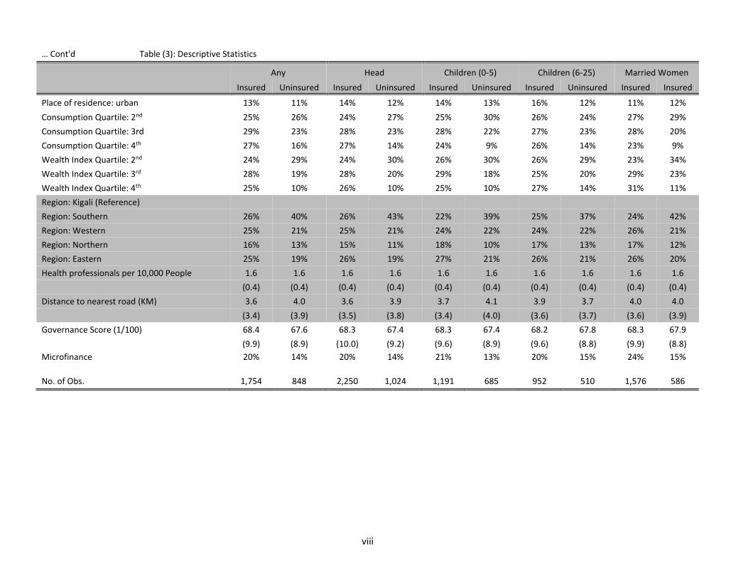
to enroll in health insurance schemes and also have better utilization rates. Table (3) summarizes

household-, individual-, and community-level factors which influence enrollment decisions as well as

the potential healthcare utilization outcomes. In our formal estimation of treatment effects in Section

(3), we control for demographic factors including age, gender and marital status of the head, household

size, relationship to the head, and the number of children in the household. Similarly, we control for

socio-economic factors including education and occupation of the head, and consumption and wealth

quartiles. While consumption quartiles are constructed from the annual total consumption expenditure

per capita, which is a good proxy for income, wealth quartiles are constructed from a composite wealth

index7. Community-level and regional factors include distance to the nearest road in kilometers (KM),

location of residence, the number of health professionals per 10,000 people at the district level, and

regional dummies.

3.4. Instrumental Variables

For the purpose of identification, we include two instrumental variables: (i) district-level governance

and justice performance score obtained from administrative records and (ii) a dummy variable

indicating household participation in microfinance institutions. The governance and justice

performance score (0 to 100 points) is obtained from annual reports of the Ministry of Local

Governments of Rwanda8 (MINALOC, 2010). The governance and justice performance indicators

include the number of cases registered and assembled by local courts, functioning of joint action

development forums, and financial management including CBHI schemes. It captures the level of

transparency, accountability, and efficiency of district-level administration.

7 A composite wealth index is constructed using principal component of analysis of households’ ownership of agricultural equipment, livestock, household durables, dwelling characteristics, and size of land owned. The list of items included in the calculation of wealth index is provided in Table (13). 8 Every year since 2006, the ministries and all 30 districts in the country sign a performance contract, locally referred to as “Imihigo”, with the President of Rwanda. It is part of the government’s ongoing effort to increase performance, transparency, and fostering competition among districts for good governance, economic and social developments. The performance contract has three major components against which districts are evaluated: economic development, social development, and governance and justice. The National Evaluation Team organized by the Ministry of Local Governments evaluates and ranks each district according to its performance. The economic and social development indicators include activities in establishing saving and credit associations, rural settlements, construction of housing for vulnerable households, enrollment rates in CBHI schemes, etc.

8

The second instrument is a dummy variable indicating household participation in microfinance

activities. Microfinance associations provide savings and credit services to individuals and small-

businesses who would otherwise do not have access to the formal credit market. The underlying model

of microfinance relies on “social capital” including trust, solidarity, and cooperation. We argue that

individuals who participate in such institutions at the community level are also more likely to participate

in other community-based programs such as CBHI, which involves pecuniary contribution.

As discussed later in Section (4.2), these two instruments affect individuals’ enrollment decisions in

CBHI schemes but not healthcare utilization outcomes. The summary in Table (3) shows that

individuals who reside in districts with higher governance score have higher CBHI enrollment rates.

Similarly, individuals in microfinance-participating households have higher CBHI enrollment rates.

4. Empirical Specification

4.1. The Bayesian Potential Outcomes Model

The two important empirical issues in quantifying the causal effects of a program are selection bias and

HTEs. We address these issues in a Roy potential outcomes model using Bayesian estimation

techniques. Drawing on the works of Neyman (1923) and Fisher (1952) on potential outcomes

framework, Roy’s 1950 and 1951 models of earnings and occupational choices lay the foundation for

modern economic evaluation and sample selection methods such as Heckman’s selection (Heckman

and Sattinger, 2014). The Roy model is also similar to Rubin’s Causal Model, which is popular in the

statistics and causal inference literature. In a series of works, Robin is also the first to implement

potential outcomes model using Bayesian method (Rubin 1974; 1978; 1986; 2005a,b). With the recent

advance in MCMC simulation and data augmentation techniques, Bayesian approach is an efficient

method of estimating potential outcomes models (Li and Tobias, 2008; Chib and Hamilton, 2000).

Among the numerous advantages of Bayesian method over the frequentist methods, in the context of

causal inference, Bayesian potential outcomes model jointly addresses selection bias and HTEs in a

parsimonious way.

We now specify the model and describe the estimation algorithm. Let the 𝑖th observation insurance

status is denoted by 𝑑𝑖 which takes 0 if the individual is uninsured and 1 if insured through CBHI

scheme. Also, let 𝑦𝑖 denote the observed healthcare utilization outcome, 𝑦0𝑖 = {0,1} denote the

9

potential outcomes in the uninsured state, and 𝑦1𝑖 = {0,1} denote the potential outcome in the insured

states, where 𝑦𝑖 = 𝑑𝑖𝑦1𝑖 + (1 − 𝑑𝑖)𝑦0𝑖. Because treatment and outcome variables are binary, we

estimate joint probit models in which individual 𝑖’s health insurance enrollment and potential outcomes

equations are expressed in the following latent variable forms

𝑑𝑖∗ = 𝛽𝑑𝑤𝑖 + 𝜀𝑑𝑖,

𝑦1𝑖∗ = 𝛽1𝑥𝑖 + 𝜀1𝑖,

𝑦0𝑖∗ = 𝛽0𝑥𝑖 + 𝜀0𝑖 , (1)

where 𝑑𝑖 = 1(𝑑𝑖∗ > 0) , 𝑦1𝑖 = 1(𝑦1𝑖

∗ > 0), 𝑦0𝑖 = 1(𝑦0𝑖∗ > 0), 1(∙) is indicator operator, 𝑑𝑖

∗ is the latent

utility of participating in CBHI schemes, 𝑦1𝑖∗ is the latent potential utilization outcome in the insured

state 𝑑𝑖 = 1, 𝑦0𝑖∗ is the latent potential utilization outcome in the uninsured state 𝑑𝑖 = 0, 𝑤𝑖(1 × 𝑘𝑤) =

[𝑥𝑖 𝑧𝑖] is a vector of covariates in the participation equation, 𝑧𝑖(1 × 𝑘𝑧) is a vector of instruments to

be excluded from the potential outcomes equations, 𝑥𝑖(1 × 𝑘𝑥) is a vector of covariates in the potential

outcomes equations, {𝛽𝑑, 𝛽1, 𝛽0} are vector of coefficients, {𝜀𝑑𝑖, 𝜀1𝑖, 𝜀0𝑖} are error terms in the

participation and the potential outcomes equations. The error terms are assumed to be jointly and

normally distributed with mean zero, unit variances, and non-zero correlations given by

𝜀𝑖|𝑤𝑖, 𝑥𝑖~𝑁3(0(3×1), Σ), (2)

where Σ = [

1 𝜎𝑑1 𝜎𝑑0

𝜎𝑑1 1 𝜎10

𝜎𝑑0 𝜎10 1] is the covariance matrix and 𝜀𝑖 = (

𝜀𝑑𝑖

𝜀1𝑖

𝜀0𝑖

) is a vector of error terms. The

diagonal elements of Σ are restricted to ones for the sake of identification in the probit model.

Endogeneity in CBHI enrolment is captured through correlation terms in the covariance matrix, 𝜎𝑑1

and 𝜎𝑑0. Since 𝜎10 does not enter the likelihood function, it can only be identified through learning in

the MCMC simulation (Poirier, 1998; Li and Tobias, 2005; Poirier and Tobias, 2003). Assuming

conditional independence, the likelihood function is then given by

𝑝(𝑦, 𝑑|𝑤, 𝑥, Θ) = ∏ 𝑝(𝑦1𝑖 = 𝑦𝑖, 𝑑𝑖 = 1|𝑤𝑖, 𝑥𝑖 , Θ)

𝑖:𝑑𝑖=1

∏ 𝑝(𝑦0𝑖 = 𝑦𝑖, 𝑑𝑖 = 0|𝑤𝑖, 𝑥𝑖 , Θ)

𝑖:𝑑𝑖=0

, (3)

where Θ = [𝛽𝑑 𝛽1 𝛽0 Σ ]. Then data augmentation technique is used to expand the likelihood function

in equation (4) (Tanner and Wong, 1987; Albert and Chib, 1993). In data augmentation, the latent

variables corresponding to the health insurance enrollment and potential utilization outcomes equations

10

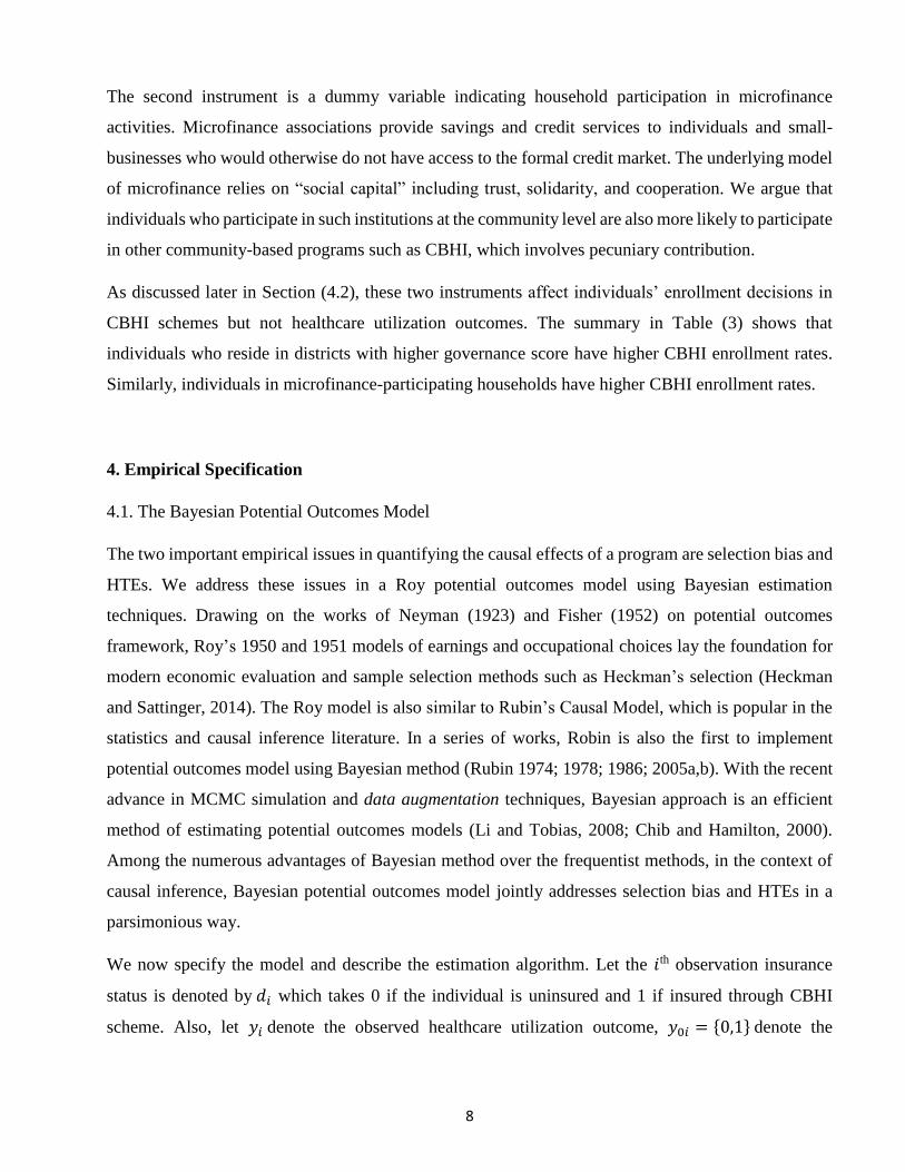
enter the likelihood function and are treated as additional parameters to be estimated alongside other

parameters. Then, the posterior distribution of parameters, which is proportional to the product of the

likelihood function and the priors, can be written as

𝑝(Θ, 𝑑∗, 𝑦1∗, 𝑦0

∗|𝑦, 𝑑, 𝑤, 𝑥, ) ∝ 𝑝(𝑦, 𝑑|Θ, 𝑑∗, 𝑦1∗, 𝑦0

∗, 𝑤, 𝑥, )𝑝(𝑑∗, 𝑦1∗, 𝑦0

∗|Θ)𝑝(Θ), (4)

The set of parameters to be estimated in our model are 𝛽 = [𝛽𝑑 𝛽1 𝛽0] and the three off-diagonal

elements of Σ. To complete the model, we specify the prior distribution for model parameters to be

non-informative conjugate distribution with 𝛽0~𝑁(𝜇𝛽0= 0, 𝑉𝛽0

= 103𝐼). Since the distribution of Σ

is not from a known family, we use MH algorithm proposed by Chan and Jeliazkov (2009). Their

approach decomposes Σ into its lower triangular and diagonal components given by {𝑎1, 𝑎2, 𝑎3}, which

is easier to draw. We also adopt a prior distribution of 𝑎𝑘~𝑁2(0, 𝐼) for 𝑎𝑘 (see Chan and Jeliazkov

(2009) for details and Appendix A for a short note.)

Summary of the algorithm to draw parameters of the model from their conditional distributions is

presented in Box 1. Details of the estimation algorithm are given in Appendix A.

Box 1: Estimation Algorithm: Binary Treatment and Binary Outcomes

Step 0: Initialize parameters

Step 1: Draw 𝛽 independently from its conditional distribution

Step 2: Draw 𝑎 = [𝑎21 𝑎31 𝑎32] independently from its conditional

distribution using Chan and Jeliazkov (2009) Metropolis-

Hastings (MH) algorithm with multivariate normal proposal

Step 3: Draw 𝑑∗ independently from its conditional distribution

Step 4: Draw 𝑦1∗ independently from its conditional distribution

Step 5: Draw 𝑦0∗ independently from its conditional distribution

Cycling through steps 1 to 5 until convergence yields the posterior parameter estimates. The estimation

code is written in Matlab9 and tested on simulated data with known parameters before we apply it to

the real data. We conduct convergence diagnosis using trace plots of the draws and formal convergence

diagnostic test developed by Geweke (1992). We draw 10,000 MCMC iterations with first 5,000 draws

dropped as burn-in10.

9 We used Chan and Jeliazkov (2009) matlab code to draw the covariance matrix. 10 Trace plots and Geweke convergence diagnostic tests can be obtained from the authors.

11

4.2. Identification

The model is identified from two sources: (i) the economics of the Roy model, and (ii) exclusion

restriction.

4.2.1. Economics of the Roy model – Self-Selection

The Roy model has rich economic content providing information for empirical identification of the

model. In a nonrandomized setting, individuals participate in a program if the expected utility from

participating outweighs the expected utility from not participating in the program, i.e. 𝑑𝑖 =

1[𝑦𝑖1 > 𝑦𝑖0]. In the contrary, under randomized control approach, individuals are placed into different

treatment states through exogenous randomization mechanism and they are not presented with the

option of making a decision on their treatment status. Such exogenous treatment assignment mechanism

subdues the information content on individuals’ revealed preference (Heckman, 2005). In the Roy

model, self-selection is one source of information on individuals’ revealed preferences linking the

potential outcomes with participation decisions. Individuals are assumed to make participation

decisions based on their expected utilities. This is called the economic content of the Roy model which

helps in model identification (Heckman and Smith, 1998; Heckman and Honore, 1990).

The Roy model is identified without exclusion restriction under the condition that 𝑋 ⊥ (𝜀1𝑖, 𝜀0𝑖) and

finite variances (Heckman and Smith, 1998). In the context of skills and earnings distributions,

Heckman and Honore (1990) show that the normal version of the model is identifiable from a cross-

section data without the need for exclusion restriction or regressors (Heckman, 1974a, b). Heckman

and Smith (1998) discuss identification of the Roy model and how individuals’ participation decisions

reveal information that helps identify the model. Recently, Li, Poirier and Tobias (2004) and Li and

Tobias (2008) implemented the Roy model using Bayesian estimation technique without exclusion

restriction. Similarly, Eisenhauer et al. (2014) extended the Roy model to estimate cost and benefit

parameters through variation in cost shifters.

4.2.2. Exclusion Restriction – Instrumental Variables

Our instrumental variables are the 2009/2010 district-level governance and justice performance score

and households’ participation in microfinance activities. One of the criteria for identification through

exclusion restriction is that the excluded variable/s should significantly affect enrollment decision but

not the outcome variables. Our instruments meet such criteria and are validated through a battery of

12

overidentification tests in a classical two-stage estimation framework11. The test results (p-values

associated with the Amemiya-Lee-Newey minimum Chi-Square statistics), presented in Table (4),

show that the model is overidentified for all models of healthcare utilization and sub-samples, providing

strong support for the validity of the instruments.

Governance and justice scores should capture the level of trust and individuals’ perceptions about the

local administrations which manage and coordinate CBHI activities including enrollment, collection of

premiums, finances, and overall operations. We anticipate that individuals who reside in districts with

poor financial management, corruption, and injustice are reluctant to enroll in CBHI schemes than

individuals in districts with good governance. Similarly, households’ participation in microfinance

activities should be picking up their perception and willingness to participate in community-based

activities. Those who participate in microfinance activities are more familiar with community-based

schemes, especially those involving pecuniary contribution, and are also more likely to enroll in CBHI

schemes.

4.3. Treatment Effects

For each individual, the causal effects of CBHI on the probability of utilizing a healthcare service is

defined as

𝑖𝑇𝐸(𝑋; 𝜃) ≡ 𝐸𝜃[Pr(𝑦1𝑖 = 1|𝑋 = 𝑥; 𝜃) − Pr(𝑦0𝑖 = 1|𝑋 = 𝑥; 𝜃)]. (5)

Then, by integrating over model parameters, 𝑖𝑇�̂�(𝑋) is computed using post-convergence parameter

values from MCMC simulations as follows

𝑖𝑇�̂�(𝑥) = 𝐸𝜃[𝑖𝑇𝐸(𝑋; 𝜃)] ≈1

𝑅∑ 𝑖𝑇𝐸(𝑋; �̃�𝑅)

𝑅

𝑟=1

, (6)

where 𝐸𝜃 is expectation operator over the parameter vector 𝜃, �̃�𝑅 is a vector of post-convergence model

parameters obtained from the MCMC chains. Equation (6) gives us the whole distribution of treatment

effects for the sample from which we can obtain the ATEs and ATTs12 by averaging over observations.

11 Specifically, we used ivprobit command followed by overid command in Stata written by Baum et al. (2006). 12

ATTs measures program gains and losses under the two treatment states for individuals who are actually treated and can

be computed as follows

𝑖𝑇𝑇(𝑋, 𝑑 = 1; 𝜃) = 𝐸𝜃[Pr(𝑦1𝑖 = 1|𝑑𝑖 = 1, 𝑋 = 𝑥; 𝜃) − Pr(𝑦0𝑖 = 1|𝑑𝑖 = 1, 𝑋 = 𝑥; 𝜃)].

13

4.4. Bayesian Model Comparison

In order to compare different models, we calculate the log marginal likelihood using a method

developed by Chib (1995). The log marginal likelihood is obtained by integrating the sampling density

over the prior density. Formally, the log marginal likelihood is defined by

ln 𝑚(𝑑, 𝑦|𝑋) = ln 𝑓(𝑦, 𝑑|�̃�, 𝑑∗, 𝑦1∗, 𝑦0

∗, 𝑋) + ln 𝑝(�̃�) − ln 𝑝(�̃�, 𝑑∗, 𝑦1∗, 𝑦0

∗|𝑦, 𝑑, 𝑋),

where ln 𝑚(𝑑, 𝑦|𝑋) is the log of marginal likelihood, �̃� is a vector of posterior parameter estimates

obtained from the MCMC iterations. The first RHS term is the log-likelihood and the second term is

log of the prior distribution evaluated at the post-convergence parameter values, which are readily

available from the MCMC runs. The third term on the other hand can be calculated by partitioning the

parameters into several components and integrate over the latent variables, {𝑑∗, 𝑦1∗, 𝑦0

∗}, which are the

byproducts of the MCMC runs and are readily available. In our case, we decompose the posterior

parameter distribution into two blocks: a vector of slope parameters in one black and the covariance

matrix in another, i.e. 𝑝(𝛽,̃ Σ,̃ |𝑑∗, 𝑦1∗, 𝑦0

∗, 𝑤, 𝑥) = 𝑝(𝛽|Σ,̃ 𝑑∗, 𝑦1∗, 𝑦0

∗, 𝑤, 𝑥)𝑝(Σ̃|𝑑∗, 𝑦1∗, 𝑦0

∗, 𝑤, 𝑥).

5. Results and Discussions

First, we discuss estimated parameters of the enrollment and the potential healthcare utilization

outcomes equations. Then, we discuss results on the causal effects of CBHI on healthcare utilization.

The estimation is done for five groups of individuals: (i) randomly selected household members, (ii)

heads of households, (iii) children under the age of five, (iv) children between the age of 6 and 25, and

(v) married women (spouses).

5.1. CBHI enrollment, selection, and potential outcomes

In order to address selection bias on observables, we include individual- and household-level

demographic and socio-economic characteristics, consumption and wealth quintiles, and access to

Integrating over the posterior parameter values in a similar fashion as before we have

𝑖𝑇�̂�(𝑋, 𝑑 = 1) = 𝐸𝜃[𝑖𝑇𝑇(𝑋, 𝑑 = 1; 𝜃)] ≈1

𝑅∑ 𝑖𝑇𝑇(𝑋, 𝑑 = 1; �̃�𝑅)

𝑅

𝑟=1

.

The treatment effect on the untreated (ATUT) can be computed in a similar fashion for the uninsured individuals in the

sample. Li and Tobias (2008) shows details of how 𝑖𝑇𝑇 and 𝑖𝑇𝑈𝑇 are derived for an ordered probit which can easily be

adopted for the simple probit model.

14

healthcare facilities as well as geographic and area-level factors in the model. Then, we address

selection on unobservable factors by allowing the error terms in the system of enrollment and potential

outcomes equations (in equation (1)) to be correlated. The estimated correlations measure the

magnitude and significance of selection bias on unobservable factors.

Table (5) presents estimates of the coefficients in the enrollment equation for all subsamples. The

coefficients in all three healthcare utilization models (i.e., consultation, screening, and drug) are similar

in directions, magnitudes, and statistical significances. Hence, for the sake of brevity, we discuss

estimated coefficients obtained from the enrollment and the utilization of consultation equations only.

5.1.1. Household demographic characteristics

The results show that some household demographic characteristics significantly affect individuals’

health insurance enrollment decisions. Married household heads are more likely to enroll their family

members in CBHI schemes including themselves. While male household heads are less likely to enroll

compared to females, sex of the head is not a significant factor for enrollment of other household

members. Similarly, age of the head is not a significant factor in the enrollment of household members

except for under-five children. Another observation is that the likelihood of children and married

women to be enrolled in CBHI schemes significantly decreases when the number of children in the

household increases. This implies that there is intra-household competition, perhaps systematic

rationing, in terms of who gets enrolled in CBHI. Furthermore, male household members, biological

children and members who have other relationships with the head are less likely to be enrolled

compared to the head.

When it comes to socio-economic factors, education has no statistically significant impact on

enrollment decisions. For instance, family members headed by uneducated heads are as much likely to

enroll as members head by educated heads. However, occupation significantly affects enrollment where

heads of households who are primarily engaged in agricultural activities are less likely to enroll their

family members than those in industry, service, and other non-agricultural sectors.

5.1.2. Budget constraint

Household budget and wealth levels play significant role in enrollment decisions since enrollees have

to pay a flat premium of 1,000 RWF per year, 10% co-pay at hospitals, and up to 200 RWF at health

centers. We anticipate that households with higher income and wealth are more likely to enroll in health

15

insurance because they can afford to pay the premium and want to insure their wealth/asset against

health-related financial shocks. In line with this argument, the results show that compared to households

in the bottom quartile, those who are in the second, third, and fourth quartiles of consumption

expenditure are more likely to enroll their family members in CBHI schemes. The other significant

financial factor is wealth where households in the top three quartiles of the distribution have

significantly higher chance of enrolling their family members.

5.1.3. Access to healthcare services

The results in Table (5) show that distance to the nearest road does not significantly affect the likelihood

of enrollment except for children between the age of 6 and 25. On the contrary, the coefficient on

district-level number of health professionals per 10,000 people is negative and statistically significant

for all but children between the age of 6 and 25, which seems counter-intuitive. In terms of regional

differences, compared to Kigali (the capital city of Rwanda), residents in the southern region, which

borders with Burundi, are less likely to enroll in CBHI schemes. The two exogenous variables,

governance score and participation in microfinance activities, significantly increase the chance of

CBHI enrollment further validating our choice of instruments.

5.1.4. Potential utilization outcomes

In the Bayesian potential outcomes framework, we can estimate the potential outcomes quantities,

which are byproducts of the MCMC simulations. Since an individual cannot be observed in the insured

and the uninsured states at the same time, the potential outcomes (i.e., 𝑃𝑂1 = 𝐸𝜃[Pr(𝑦1𝑖 = 1|𝑑𝑖 =

1, 𝑋 = 𝑥; 𝜃)] and 𝑃𝑂0 = 𝐸𝜃[Pr(𝑦1𝑖 = 1|𝑑𝑖 = 1, 𝑋 = 𝑥; 𝜃)]) are simulated conditional on the data,

model structure, and the parameters. Table (7) presents estimates of the potential utilization

probabilities under the insured and the uninsured states. In addition, we graphically present the whole

distribution of the potential probabilities of utilizing healthcare services in Figure (2). The results show

that, for all healthcare services and groups of individuals under consideration, the potential probabilities

of healthcare utilization outcomes under the insured state are higher than utilization rates under the

uninsured state. Except utilization of screening services, the estimated potential utilization quantities

are significantly different from zero under the uninsured state.

Factors other than CBHI also affect the potential healthcare utilization outcomes. Tables (10)-(12)

present the estimated coefficients of the potential utilization equations. For instance, while the presence

of children aged 6-25 in the household and age have significant negative impact on the probability of

16

consulting medical professionals under the insured state, wealth has significantly positive impact.

Under the uninsured state, marital status of the head, income and district-level density of healthcare

professionals have significant impact on the utilization of consultation services. Notice that, for under-

five children, regardless of insurance status, as age increases, the potential probability of consultation

decreases significantly.

In general, the results in Table (5) and Tables (10)-(12) underscore the importance of selection on

observables where demographic factors, income, wealth, and distance to road significantly affect the

potential utilization probabilities and CBHI enrollment decisions. In addition, the levels of selection on

observables considerably vary across individuals and healthcare services.

5.1.5. Selection on unobservables

One of the advantages of Bayesian potential outcomes model is that we can estimate the correlation

matrix, which captures selection bias arising from unobserved factors. If there is selection bias on

unobservables, then the correlation coefficients should be significantly different from zero. Table (6)

presents the posterior estimates of the correlation coefficients for all models of healthcare utilization

and groups of individuals. In all cases, the estimated correlations are economically and statistically

insignificant implying no systematic bias arising from factors unobserved to the researchers.

5.3. Causal inference

5.3.1. Average Treatment Effects

We now turn to the discussion of causal effects of CBHI on the probability of utilizing healthcare

services. While Table (8) presents posterior estimates of ATEs13, Figure (2a) and Figure (2b) show the

distribution of estimated individual-level treatment effects and district-level ATEs. The results show

that CBHI has significant impact in increasing the utilization of consultation services for all household

members with varying magnitude. In particular, the program has the highest impact on the most

vulnerable members of society, married women and under-five children. Those with CBHI coverage

realize the highest benefits in terms of receiving consultation and screening services. CBHI increases

the likelihood of receiving consultation for married women and under-five children by 32 and 31

percentage points, respectively. Similarly, it significantly increases the likelihood of receiving

13 ATTs and ATUTs are also estimated but not reported for the sake of brevity.

17

consultation services for randomly selected family members, children aged 6-25, and heads of

households by 28, 27, and 26 percentage points, respectively. With regards to utilization of screening

services, CBHI increases utilization probabilities by 18 percentage points for married women and

under-five children by 15 percentage points for heads of households. However, the impact is not

statistically significant for randomly selected family members and children aged 6-26.

In the case of drug utilization, CBHI does not have statistically significant effect for all groups of

individuals in our sample. The result is not surprising because CBHI covers only essential drugs, which

are provided at health centers and hospitals. As utilization of non-essential drugs involves direct out-

of-pocket expenditure irrespective of insurance status, we do not expect strong impact on drug and

medical supplies purchases due to CBHI. If there is any impact on drug utilization, it could be indirectly

through budget and preference shifts. Because, insured individuals pay premiums and receive

healthcare services at a reduced price, whereas the uninsured do not pay premiums but pay higher prices

in times of illness to receive care. The net budgetary effect could be either positive or negative

depending on the magnitude of illness or healthcare needs. The other potential channel through which

CBHI could affect drug utilization is preference shift. If insured individuals are more likely to visit

healthcare providers, they are more likely to get prescriptions or persuaded to purchase drugs.

5.3.2. Heterogeneous treatment effects

Individuals behave and respond to treatments differently due to differences in preferences, budget

constraints, and environmental factors such as access to healthcare facilities. As a result, we expect the

treatment effects to be heterogeneous. It is difficult to understand the degree of heterogeneity in

treatment effects from the standard ATEs estimates. One advantage of our approach over the classical

evaluation techniques is its flexibility to estimate treatment effects for each person, which can then be

summarized or visualized in various fashions.

Figure (2a) shows histograms of the estimated individual-level treatment effects for each sub-sample

and utilization of healthcare services. In general, had a treatment effect been homogenous, we would

have observed a degenerate distribution which is also the ATE. However, the figures show that there

is considerable heterogeneity in treatment effects across individuals, the type of healthcare service, and

intra-household subgroups.

18

For instance, the impact of CBHI on utilization of consultation services for randomly selected family

members range from 18.5 to 59.8 percentage points. However, for about 98.7% of the observation, the

impact is positive. Similarly, the ranges of treatment effects on utilization of screening services and

drugs are [-19.9, 46.2] and [-15.7, 43.8] percentage points, respectively. Although we observe negative

treatment effects for some individuals, the impacts are positive for considerable proportion of

individuals in the sample. There is also significant heterogeneity in treatment effects on utilization of

drug, particularly for children between the age of 6 and 25 years. Treatment effects range from a

reduction in utilization probability by 37.4 percentage points to an increase by 57.2 percentage points.

These are wide ranges with important policy implications on targeting of CBHI schemes for different

groups of individuals.

Figure (2b) and Figure (3) shows bar plots and heat maps of ATEs by district where there is

considerable heterogeneity in treatment effects across districts. Districts which have higher ATEs on

utilization of one healthcare service are also more likely to have higher ATEs on the utilization of

another healthcare service. For instance, while Gekenke district is among the top five performers with

higher ATEs in all three healthcare utilization outcomes, Ngoma district is among the bottom five

performers. In general, the results underscore heterogeneous impacts of CBHI on healthcare utilizations

not only at the individual and intra-household levels but also at district and region levels.

5.4. Model comparison

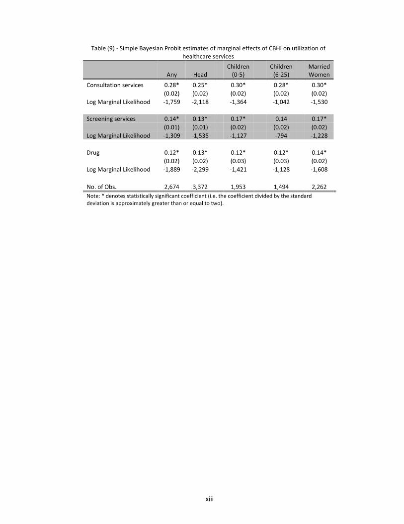
For the purpose of model comparison, we present marginal effects of enrollment in CBHI schemes on

healthcare utilization using simple Bayesian probit model (see Table (9)). Two important points warrant

a brief discussion. First, the estimated ATEs using the probit model are very close to the estimates from

the potential outcomes models. This corroborates with the results discussed in Section (5.1.5.), where

the estimated correlation coefficients show no selection bias on unobservable factors. It signifies that,

after controlling for observed factors, there is no systematic difference in the sample between the

insured and the uninsured individuals. Second, the estimated ATEs using simple probit are statistically

significant for all services and groups of individuals, which is not the case in the potential outcomes

model. The potential outcomes approach acknowledges that enrollment is endogenously determined

and handles it in a system of enrollment and potential outcomes equations.

19

As expected the log marginal likelihood of the probit model shows a much better model fit compared

to the potential outcomes model. Generally, smaller log marginal likelihood is expected when certain

structure is imposed, which is the case in the potential outcomes models with a system of enrollment

and potential outcomes equations jointly estimated. However, as noted above, the potential outcomes

model has several advantages over the simple probit model or other classical evaluation methods

addressing selection bias and HTEs in a structural framework. The take home message is that the

estimated treatment effects of CBHI on utilization rates remain robust to different model specifications.

6. Conclusion

Utilization of modern healthcare services is very low in developing countries mainly due to lack of

affordable health insurance coverage. In many places, functioning private health insurance markets are

missing and the existing public health insurance systems are not accessible for the poor. CBHI schemes

have become formidable healthcare financing alternatives providing affordable coverage for the poor

across developing countries. Rwanda has scaled up coverage of CBHI schemes from just around 35%

in 2006 to about 86% in 2008 amid uncertainty about the potential impact on healthcare utilization and

financial protection from health-related income shocks.

This study examines the impact of CBHI on utilization of healthcare services such as consultation,

screening, and drugs in case of Rwanda. We used a nationally representative data from nonrandomized

household survey addressing issues of selection bias and HTEs in a Bayesian potential outcomes

framework with data augmentation and MCMC simulation techniques. By recovering potential

utilization outcomes and treatment effects at the individual level, we graphically present the whole

distribution of treatment effects. In order to address intra-household heterogeneity, the analysis is

conducted for five groups of individuals (randomly selected individuals, heads of households, children

aged 0-5, children aged 6-25, and married women) categorized according to their roles and relationships

in the household.

Our findings show that membership in CBHI schemes significantly increases the likelihood of utilizing

medical consultation and screening services. However, we find no significant impact on the likelihood

of purchasing drugs. Factors other than CBHI, such household demographic characteristics, income,

occupation, and geographic characteristics, significantly affect potential utilization of health care

services regardless of insurance status. Furthermore, the results show considerable HTEs at the

individual and intra-household levels. Although rapidly implemented amid uncertainty of its impact,

20

CBHI program has significantly increased utilization of key healthcare services in Rwanda with the

highest gain realized by married women and under-five children.

References

Acharya, Arnab; Vellakkal, Sukumar; Taylor, Fiona; Masset, Edoardo; Satija, Ambika; Burke,

Margaret; and Ebrahim, Shah (2012). The impact of Health Insurance Schemes for the Informal

Sector in Low- and Middle-Income Countries: A Systematic Review.

Aggarwal, A. (2010), Impact evaluation of India's ‘Yeshasvini’ community-based health insurance

programme. Health Econ., 19: 5–35. doi: 10.1002/hec.1605.

Albert, J. H. and S. Chib (1993). Bayesian analysis of binary and polychotomous response data. Journal

of the American statistical Association 88 (422), 669-679.

Albert, J. H. and S. Chib (2001). Sequential ordinal modeling with applications to survival data.

Biometrics 57 (3), 829-836.

Baum, C.F., Schaffer, M.E., Stillman, S., Wiggins, V. 2006. overid: Stata module to calculate tests of

overidentifying restrictions after ivreg, ivreg2, ivprobit, ivtobit, reg3.

http://ideas.repec.org/c/boc/bocode/s396802.html.

Binagwaho, A., Hartwig, R., Ingeri, D., & Makaka, A. (2012). Mutual health insurance and its

contribution to improving child health in Rwanda (Vol. 66, No. 12). Passauer

Diskussionspapiere: Volkswirtschaftliche Reihe.

Chan, Joshua Chi-Chun and Jeliazkov, Ivan (2009). MCMC Estimation of Restricted Covariance

Matrices. Journal of Computational and Graphical Statistics, Volume 18, Number 2, Pages 457–

480. DOI: 10.1198/jcgs.2009.08095

Chib, S. and B. H. Hamilton (2000). Bayesian analysis of cross-section and clustered data treatment

models. Journal of Econometrics 97 (1), 25-50.

Eisenhauer, Philipp; Heckman, James J.; Vytlacil, Edward (2014), The generalized Roy model and the

cost-benefit analysis of social programs, ZEW Discussion Papers, No. 14-082.

Geweke, J. (1992). Evaluating the accuracy of sampling-based approaches to the calculation of

posterior moments. Evaluating the accuracy of sampling-based approaches to calculating

posterior moments.

Heckman, J. J. (2008). Econometric causality. International Statistical Review,76(1), 1-27.

Heckman, J. J., Lopes, H. F., & Piatek, R. (2014). Treatment effects: A Bayesian

perspective. Econometric reviews, 33(1-4), 36-67. . doi:10.1080/07474938.2013.807103

Heckman, J. J. and Sattinger, M. (2015), Introduction to The Distribution of Earnings and of Individual

Output, by A.D. Roy. The Economic Journal, 125: 378–402. doi: 10.1111/ecoj.12226

ii

Jutting, J.P. (2003), “Do community-based health care insurance schemes improve poor people’s access

to health care? Evidence from rural Senegal”, World Development, Vol.32, No.2, pp. 273-288.

Li, M. and J. L. Tobias (2008). Bayesian analysis of treatment effects in an ordered potential outcomes

model. Advances in econometrics 21, 57-91.

Lu C, Chin B, Lewandowski JL, Basinga P, Hirschhorn LR, et al. (2012) Towards Universal Health

Coverage: An Evaluation of Rwanda Mutuelles in Its First Eight Years. PLoS ONE 7(6):

e39282. doi:10.1371/journal.pone.0039282

MINALOC, 2010. Reports on Districts Imihigo Evaluation Report 2009/2010. Rwandan Ministry of

Local Governments, July 2010.

Mladovsky, P. and Mossialos E. (2007), “A conceptual framework for community-based health

insurance in low-income countries: social capital and economic development”, World

Development Vol.36, no.4,pp.590-607.

MoH (2008). Health Financing Systems: Options for Universal Healthcare. World Health Orgnization

and Republic of Rwanda, Ministry of Health, 2009.

MoH (2009). Rwanda Health Financing Policy. Republic of Rwanda, Ministry of Health, December

2010.

MoH (2010). Rwanda National Health Insurance Policy. Republic of Rwanda, Ministry of Health,

December 2010.

MoH (2010). Rwanda Community Based Health Insurance Policy. Republic of Rwanda, Ministry of

Health, April 2010.

MoH (2012). Annual Report: Community Based Health Insurance. Government of Rwanda, Ministry

of Health, October 2012.

Poirier, D. J. (1998). Revising beliefs in nonidentified models. Econometric Theory 14 (04), 483-509.

Poirier, D. J. and J. L. Tobias (2003). On the predictive distributions of outcome gains in the presence

of an unidentified parameter. Journal of Business & Economic statistics 21 (2), 258-268.

Roy, A.D. (1950). ‘The distribution of earnings and of individual output’, Economic Journal,

vol. 60(239), pp. 489–505.

Roy, A.D. (1951). ‘Some thoughts on the distribution of earnings’, Oxford Economic Papers, New

Series, vol. 3(2), pp. 135–46.

Rubin, D.B. (1974). ‘Estimating causal effects of treatments in randomized and nonrandomized

studies’, Journal of Educational Psychology, vol. 66(5), pp. 688–701.

iii

Rubin, D. B. (1978). Bayesian inference for causal effects: The role of randomization. The Annals of

Statistics, 34-58.

Rubin, D. B. (1986). Statistics and causal inference: Comment: Which ifs have causal answers? Journal

of the American Statistical Association 81 (396), 961-962.

Rubin, D. B. (2005a). Bayesian inference for causal effects. In D. Dey and C. Rao (Eds.), Bayesian

Thinking Modeling and Computation, Volume 25 of Handbook of Statistics, pp. 1-16. Elsevier.

Rubin, D. B. (2005b). Causal inference using potential outcomes. Journal of the American Statistical

Association 100 (469).

Shimeles, A. (2010). Community based health insurance schemes in Africa: The case of Rwanda.

Working Papers Series No. 120, African Development Bank, Tunis, Tunisia.

Tanner, M. A. and W. H. Wong (1987). The calculation of posterior distributions by data augmentation.

Journal of the American statistical Association 82 (398), 528-540.

iv

Appendix A. Posterior Simulators of Bayesian Potential Outcome Model: Binary Treatment and

Binary Outcomes

The function given in equation (4) in the main text is equivalent to

{∏ Φ3(𝑍𝑖; 𝑋𝑖𝛽; 𝛴)

𝑛

𝑖=1

× [𝐼(𝑑𝑖 = 1)𝐼(𝑑𝑖∗ > 0)𝐼(𝑦1𝑖 = 1)𝐼(−∞ < 𝑦1𝑖

∗ < ∞)

+ 𝐼(𝑑𝑖 = 0)𝐼(𝑑𝑖∗ ≤ 0)𝐼(𝑦1𝑖 = 0)𝐼(−∞ < 𝑦0𝑖

∗ < ∞)]} 𝑝(Θ),

where 𝑍𝑖 = [𝑑∗ 𝑦1∗ 𝑦0

∗]′, 𝑋𝑖 = 𝑑𝑖𝑎𝑔(𝑤𝑖, 𝑥𝑖, 𝑥𝑖), 𝑝(Θ) is the prior on model parameters, Φ3(∙) is

trivariate cumulative density function (cdf), 𝐼(∙) is indicator function, and the term in the curly bracket

is the likelihood function. One of the challenges in the model is that the covariance matrix is not from

standard (know) family of distributions with ones on the diagonal and nonzero off-diagonals elements.

There are different approaches in the literature to draw the covariance matrix, for instance Chib (2000)

MH approach. As discussed in the main text, this paper uses the approach proposed by Chan and

Jeliazkob (2009) to draw the constrained covariance matrix. Their approach decomposes Σ into its

lower triangular and diagonal components which is easier to draw. Accordingly, let 𝐿ΣL′ = D, where

𝐿 = (1 0 0

𝑎21 1 0𝑎31 𝑎32 1

) is a lower triangular matrix and 𝐷 = 𝑑𝑖𝑎𝑔(𝜆1, 𝜆2, 𝜆3) is a diagonal matrix with

positive elements. With this parameterization, Chan and Jeliazkov expressed the restricted covariance

matrix as 𝜆1 = 1, and 𝜆𝑘 = 1 − ∑ (𝑎𝑘𝑗)2

𝜆𝑗𝑘−1𝑗=1 , 𝑘 = 2,3, and 𝜆 is a deterministic function which will

not be estimated and 𝑎𝑘𝑗 are drawn from their conditional distributions. Since the distribution is

unknown, drawing 𝑎𝑘𝑗 uses Acceptance-Rejection MH (ARMH) algorithm. We adopt prior distribution

𝑎𝑘~𝑁2(0, 𝐼) for 𝑎𝑘 (see Chan and Jeliazkov (2009) for details). Then, the detailed algorithm to draw

parameters of the model from their conditional distributions is as follows.

Step:

0. Initialize parameters

1. Draw 𝛽 from the following distribution using Gibbs sampler

𝛽|𝑍, Σ, 𝑦, 𝑑~𝑁(𝐷𝛽𝑑𝛽 , 𝐷𝛽)

where 𝐷𝛽 = [𝑋′Σ−1𝑋 + 𝑉𝛽0

−1]−1

and 𝑑𝛽 = [𝑋′Σ−1𝑍 + 𝑉𝛽0𝜇𝛽0

]

2. Draw 𝑎 = [𝑎21 𝑎31 𝑎32] using MH algorithm with multivariate normal (or multivariate-t)

proposal density denoted by 𝑓(𝑎𝑐|𝜇, 𝑉). The conditional likelihood function is given by

𝑝(𝜀|𝑟𝑒𝑠𝑡) ∝ (∏ 𝜆𝑘

−𝑁

23𝑘=1 ) 𝑒𝑥𝑝 (−

1

2∑ (𝜀𝑖 − Ε𝑖𝑎)′𝐷−1(𝜀𝑖 − Ε𝑖𝑎)𝑁

𝑖=1 ). Because of the restriction,

v

∏ 𝜆𝑘

−𝑁

23𝑘=1 is deterministic expressed in terms of 𝑎𝑘𝑗 and satisfy the condition that Σ is positive

definite matrix. Chan and Jeliazkov (2009) suggested multivariate 𝑡 distribution for candidate

distribution draw for 𝑎 but in this paper we use a simple Random Walk draw from multivariate

normal. Then draw posterior of 𝑎 by setting 𝑎(𝑡) to 𝑎𝑐 using moving MH probability

𝑚𝑖𝑛 {1,𝑝(𝜀|Σ𝑐, 𝑟𝑒𝑠𝑡)𝑝(𝑎𝑐)𝐼(𝜆𝑐 > 0)𝑓(𝑎(𝑡−1)|𝜇, 𝑉)

𝑝(𝜀|Σ(𝑡−1), 𝑟𝑒𝑠𝑡)𝑝(𝑎(𝑡−1))𝐼(𝜆(𝑡−1) > 0)𝑓(𝑎𝑐|𝜇, 𝑉)}.

3. Draw 𝑑𝑖∗ independently from its conditional truncated normal distribution

𝑑𝑖∗|𝑦1

∗, 𝑦0∗, 𝛽, Σ, 𝑦, 𝑑~ {

𝑇𝑁(−∞,0)(𝜇𝑑𝑐 , 𝜎𝑑

𝑐) 𝑖𝑓 𝑑𝑖 = 0

𝑇𝑁(0,∞)(𝜇𝑑𝑐 , 𝜎𝑑

𝑐) 𝑖𝑓 𝑑𝑖 = 1

where 𝜇𝑑𝑐 = 𝛽𝑑𝑤 + Σ1𝑗Σ𝑗𝑗

−1(𝑧𝑗∗ − 𝛽𝑗𝑋𝑗) and 𝜎𝑑

𝑐 = Σ11 − Σ1𝑗Σ𝑗𝑗−1Σ′1𝑗.

4. Draw 𝑦1𝑖∗ independently from its conditional distributions

𝑦1𝑖∗ |𝑑𝑖

∗, 𝑦0∗, 𝛽, Σ, 𝑦, 𝑑~ {

𝑁(𝜇𝑦1𝑐 , 𝜎𝑦1

𝑐 ) 𝑖𝑓 𝑑𝑖 = 0

𝑇𝑁(𝑡𝑟𝑢𝑛𝑐)(𝜇𝑦1𝑐 , 𝜎𝑦1

𝑐 ) 𝑖𝑓 𝑑𝑖 = 1

where 𝜇𝑦1𝑐 = 𝛽1𝑥 + Σ2𝑗Σ𝑗𝑗

−1(𝑧𝑗∗ − 𝛽𝑗𝑋𝑗) , 𝜎𝑦1

𝑐 = Σ22 − Σ2𝑗Σ𝑗𝑗−1Σ′2𝑗, 𝑡𝑟𝑢𝑛𝑐 = (−∞, 0) if 𝑦𝑖 = 0

and 𝑑𝑖 = 1, and 𝑡𝑟𝑢𝑛𝑐 = (0, ∞) if 𝑦𝑖 = 1 and 𝑑𝑖 = 1.

5. Draw 𝑦0𝑖∗ independently from its conditional distributions

𝑦0𝑖∗ |𝑑𝑖

∗, 𝑦1∗, 𝛽, Σ, 𝑦, 𝑑~ {

𝑇𝑁(𝑡𝑟𝑢𝑛𝑐)(𝜇𝑦0𝑐 , 𝜎𝑦0

𝑐 ) 𝑖𝑓 𝑑𝑖 = 0

𝑁(𝜇𝑦0𝑐 , 𝜎𝑑0

𝑐 ) 𝑖𝑓 𝑑𝑖 = 1

where 𝜇𝑦0𝑐 = 𝛽0𝑥 + Σ3𝑗Σ𝑗𝑗

−1(𝑧𝑗∗ − 𝛽𝑗𝑋𝑗) , 𝜎𝑦0

𝑐 = Σ33 − Σ3𝑗Σ𝑗𝑗−1Σ′3𝑗, 𝑡𝑟𝑢𝑛𝑐 = (−∞, 0) if 𝑦𝑖 = 0

and 𝑑𝑖 = 0, and 𝑡𝑟𝑢𝑛𝑐 = (0, ∞) if 𝑦𝑖 = 1 and 𝑑𝑖 = 0.

Cycle through steps 1-5 until convergence.

Appendix B. Tables and Figures

Table (1): The percentage of individuals by the health insurance type

Health Insurance

The whole sample Randomly selected household members

Any Heads Children

(0-5) Children

(6-25) Married Women Any Head

Children (0-5)

Children (6-25)

Married Women

RAMA 2.5 2.8 2.6 2.1 3.2 2.2 n.a 2.5 1.7 3.2

Mutual 64.7 64.9 61.9 64.6 69.1 64.5 n.a 63.0 64.5 69.1

CBHI 0.1 0.2 0.1 0.1 0.1 0.1 n.a 0.1 0.0 0.1

MMI 0.6 0.8 0.9 0.4 0.9 0.6 n.a 0.8 0.4 0.9

Other 0.5 0.7 0.4 0.5 0.6 0.5 n.a 0.4 0.4 0.6

Uninsured 31.5 30.6 34.1 32.5 26.2 32.2 n.a 33.1 33.0 26.2

No. of Obs. 68,385 14,303 12,279 32,322 9,483 14,306 8,347 12,314 9,480

Ill in the past two weeks

Illness prevalence 17.5 23.6 22.6 11.0 23.9 19.1 n.a. 23.1 11.8 23.9

RAMA 2.1 1.5 2.7 1.7 2.9 1.6 n.a 2.6 0.8 2.9

CBHI 64.4 66.7 59.8 63.1 69.7 64.4 n.a 61.3 64.3 69.7

Employer 0.1 0.2 0.1 0.1 0.2 0.1 n.a 0.1 0.1 0.2

MMI 0.7 0.4 1.2 0.7 0.9 0.6 n.a 1.1 0.6 0.9

Other 0.5 0.8 0.4 0.5 0.4 0.5 n.a 0.5 0.4 0.4

Uninsured 32.1 30.4 35.8 34.0 25.9 32.8 n.a 34.3 33.8 25.9

No. of Obs. 11,944 3,373 2,772 3,566 2,264 2,727 1,925 1,448 2,263

Note: RAMA = Rwandaise d’Assurance Maladie (Rwandan Health Insurance Scheme for the public sector employees); CBHI= Community Based Health Insurance; MMI = Military Medical Insurance for the service men, Employer = Non-public sector employment based health insurance, Other = Other health insurance

Table (2): Healthcare utilization rates by health insurance status

Insurance Status Any Head

Children (0-5)

Children (6-25)

Married Women

Consultation services CBHI 48% 43% 60% 48% 51%

Uninsured 15% 13% 25% 17% 14%

Screening services CBHI 23% 21% 29% 23% 26%

Uninsured 5% 4% 9% 6% 5%

Drugs CBHI 49% 45% 58% 50% 49%

Uninsured 33% 28% 41% 35% 30%

No. of Obs. 2,602 3,274 1,876 1,462 2,162

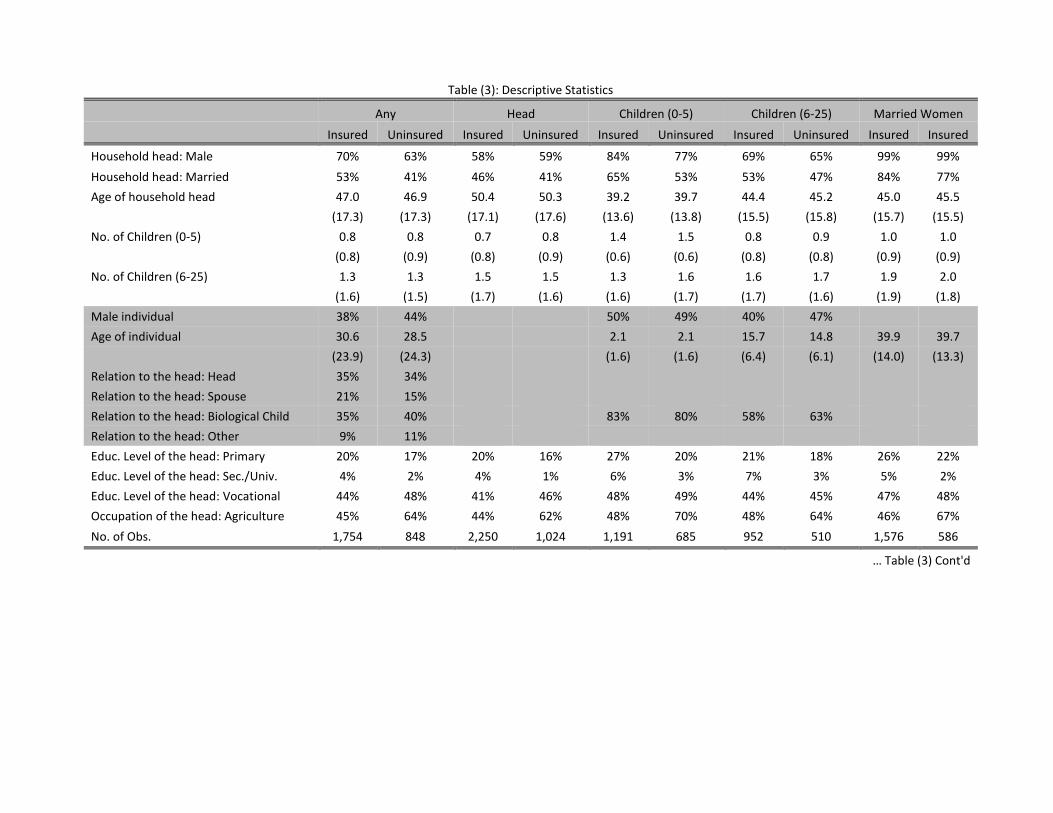
Table (3): Descriptive Statistics

Any Head Children (0-5) Children (6-25) Married Women

Insured Uninsured Insured Uninsured Insured Uninsured Insured Uninsured Insured Insured

Household head: Male 70% 63% 58% 59% 84% 77% 69% 65% 99% 99%

Household head: Married 53% 41% 46% 41% 65% 53% 53% 47% 84% 77%

Age of household head 47.0 46.9 50.4 50.3 39.2 39.7 44.4 45.2 45.0 45.5

(17.3) (17.3) (17.1) (17.6) (13.6) (13.8) (15.5) (15.8) (15.7) (15.5)

No. of Children (0-5) 0.8 0.8 0.7 0.8 1.4 1.5 0.8 0.9 1.0 1.0

(0.8) (0.9) (0.8) (0.9) (0.6) (0.6) (0.8) (0.8) (0.9) (0.9)

No. of Children (6-25) 1.3 1.3 1.5 1.5 1.3 1.6 1.6 1.7 1.9 2.0

(1.6) (1.5) (1.7) (1.6) (1.6) (1.7) (1.7) (1.6) (1.9) (1.8)

Male individual 38% 44% 50% 49% 40% 47%

Age of individual 30.6 28.5 2.1 2.1 15.7 14.8 39.9 39.7

(23.9) (24.3) (1.6) (1.6) (6.4) (6.1) (14.0) (13.3)

Relation to the head: Head 35% 34%

Relation to the head: Spouse 21% 15%

Relation to the head: Biological Child 35% 40% 83% 80% 58% 63%

Relation to the head: Other 9% 11%

Educ. Level of the head: Primary 20% 17% 20% 16% 27% 20% 21% 18% 26% 22%

Educ. Level of the head: Sec./Univ. 4% 2% 4% 1% 6% 3% 7% 3% 5% 2%

Educ. Level of the head: Vocational 44% 48% 41% 46% 48% 49% 44% 45% 47% 48%

Occupation of the head: Agriculture 45% 64% 44% 62% 48% 70% 48% 64% 46% 67%

No. of Obs. 1,754 848 2,250 1,024 1,191 685 952 510 1,576 586

… Table (3) Cont'd

viii

… Cont'd Table (3): Descriptive Statistics

Any Head Children (0-5) Children (6-25) Married Women

Insured Uninsured Insured Uninsured Insured Uninsured Insured Uninsured Insured Insured

Place of residence: urban 13% 11% 14% 12% 14% 13% 16% 12% 11% 12%

Consumption Quartile: 2nd 25% 26% 24% 27% 25% 30% 26% 24% 27% 29%

Consumption Quartile: 3rd 29% 23% 28% 23% 28% 22% 27% 23% 28% 20%

Consumption Quartile: 4th 27% 16% 27% 14% 24% 9% 26% 14% 23% 9%

Wealth Index Quartile: 2nd 24% 29% 24% 30% 26% 30% 26% 29% 23% 34%

Wealth Index Quartile: 3rd 28% 19% 28% 20% 29% 18% 25% 20% 29% 23%

Wealth Index Quartile: 4th 25% 10% 26% 10% 25% 10% 27% 14% 31% 11%

Region: Kigali (Reference)

Region: Southern 26% 40% 26% 43% 22% 39% 25% 37% 24% 42%

Region: Western 25% 21% 25% 21% 24% 22% 24% 22% 26% 21%

Region: Northern 16% 13% 15% 11% 18% 10% 17% 13% 17% 12%

Region: Eastern 25% 19% 26% 19% 27% 21% 26% 21% 26% 20%

Health professionals per 10,000 People 1.6 1.6 1.6 1.6 1.6 1.6 1.6 1.6 1.6 1.6

(0.4) (0.4) (0.4) (0.4) (0.4) (0.4) (0.4) (0.4) (0.4) (0.4)

Distance to nearest road (KM) 3.6 4.0 3.6 3.9 3.7 4.1 3.9 3.7 4.0 4.0

(3.4) (3.9) (3.5) (3.8) (3.4) (4.0) (3.6) (3.7) (3.6) (3.9)

Governance Score (1/100) 68.4 67.6 68.3 67.4 68.3 67.4 68.2 67.8 68.3 67.9

(9.9) (8.9) (10.0) (9.2) (9.6) (8.9) (9.6) (8.8) (9.9) (8.8)

Microfinance 20% 14% 20% 14% 21% 13% 20% 15% 24% 15%

No. of Obs. 1,754 848 2,250 1,024 1,191 685 952 510 1,576 586

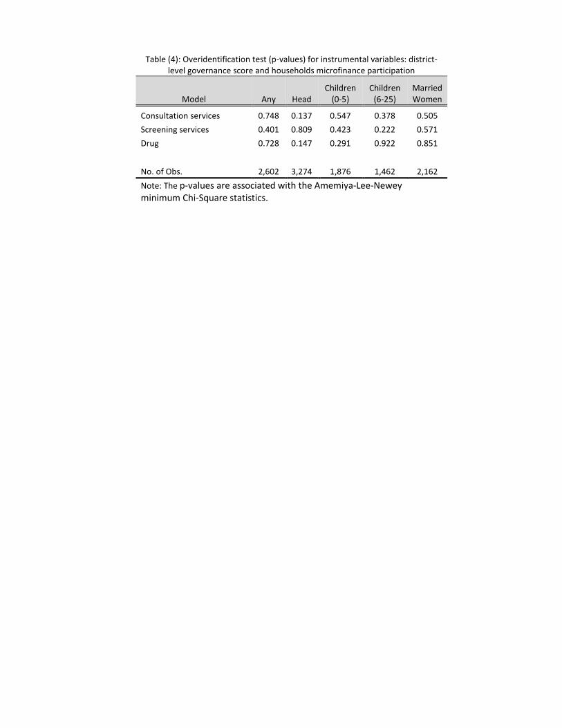
Table (4): Overidentification test (p-values) for instrumental variables: district-level governance score and households microfinance participation

Model Any Head Children

(0-5) Children

(6-25) Married Women

Consultation services 0.748 0.137 0.547 0.378 0.505

Screening services 0.401 0.809 0.423 0.222 0.571

Drug 0.728 0.147 0.291 0.922 0.851

No. of Obs. 2,602 3,274 1,876 1,462 2,162

Note: The p-values are associated with the Amemiya-Lee-Newey minimum Chi-Square statistics.

x

Table (5): Estimated parameters of the health insurance enrollment equation

(1) (2) (3) (4) (5)

Variables

Any Head Children (0-5) Children (6-25) Married Women

Mean Std. Dev. Mean

Std. Dev. Mean

Std. Dev. Mean

Std. Dev. Mean

Std. Dev.

Intercept -0.09 (0.34) 0.37 (0.30) -0.60 (0.44) -0.48 (0.46) 0.85* (0.39)

Household head: Male -0.01 (0.09) -0.33* (0.07) -0.11 (0.11) -0.13 (0.11)

Household head: Married 0.24* (0.08) 0.31* (0.07) 0.24* (0.08) 0.20* (0.10)

Household head: Age 0.004 (0.003) -0.002 (0.002) 0.01* (0.004) -0.003 (0.003)

No. of children aged 0-5 -0.05 (0.04) -0.05 (0.03) -0.16* (0.05) -0.08 (0.05) -0.01 (0.04)

No. of children aged 6-25 -0.02 (0.02) -0.01 (0.02) -0.09* (0.02) -0.03 (0.03) -0.04* (0.02)

Male -0.17* (0.07) 0.02 (0.06) -0.18* (0.07)

Age -0.01 (0.003) 0.02 (0.02) 0.01 (0.01) -0.001 (0.002)

Relation to the Head: Spouse -0.06 (0.10) Relation to the Head: Biological Child -0.39* (0.13) 0.20 (0.12) 0.08 (0.11)

Relation to the Head: Other -0.48* (0.16)

Education: Primary -0.07 (0.09) 0.02 (0.08) 0.11 (0.10) 0.05 (0.11) 0.03 (0.09)

Education: Second/University -0.09 (0.17) 0.32 (0.17) -0.03 (0.18) 0.16 (0.21) 0.13 (0.21)

Education: Vocational -0.08 (0.07) -0.09 (0.06) 0.07 (0.09) 0.02 (0.09) 0.01 (0.08)

Occupation: Agriculture -0.23* (0.06) -0.20* (0.05) -0.27* (0.08) -0.17* (0.08) -0.27* (0.07)

Place of Residence: urban 0.16 (0.10) -0.04 (0.09) 0.03 (0.12) 0.25 (0.14) -0.13 (0.12)

Cons. Quartile: Second 0.25* (0.08) 0.16* (0.07) -0.01 (0.09) 0.29* (0.10) 0.16* (0.08)

Cons. Quartile: Third 0.29* (0.08) 0.26* (0.07) 0.15 (0.09) 0.31* (0.10) 0.32* (0.09)

Cons. Quartile: Fourth 0.38* (0.10) 0.39* (0.09) 0.46* (0.13) 0.41* (0.13) 0.43* (0.12)

Wealth Quartile: Second 0.15* (0.07) 0.15* (0.06) 0.27* (0.08) 0.18* (0.09) 0.08 (0.09)

Wealth Quartile: Third 0.41* (0.08) 0.40* (0.07) 0.50* (0.10) 0.32* (0.11) 0.37* (0.09)

Wealth Quartile: Fourth 0.63* (0.10) 0.59* (0.09) 0.62* (0.13) 0.44* (0.13) 0.68* (0.12)

Distance to Road (KM) -0.01 (0.01) -0.003 (0.01) -0.004 (0.01) 0.02* (0.01) 0.01 (0.01)

Health Professionals -0.26* (0.10) -0.44* (0.09) -0.40* (0.12) -0.18 (0.14) -0.59* (0.12)

Region: Eastern 0.37* (0.14) 0.01 (0.13) 0.29 (0.17) 0.40* (0.19) 0.0001 (0.18)

Region: Western 0.19 (0.16) -0.28 (0.15) -0.01 (0.19) 0.27 (0.22) -0.21 (0.20)

Region: Northern 0.14 (0.18) -0.28 (0.17) 0.22 (0.21) 0.33 (0.24) -0.25 (0.22)

Region: Southern -0.19 (0.16) -0.72* (0.15) -0.43* (0.19) -0.09 (0.22) -0.80* (0.20)

Governance score 0.01* (0.003) 0.02* (0.003) 0.016* (0.004) 0.01* (0.004) 0.01* (0.004)

Microfinance participation 0.13* (0.07) 0.15* (0.07) 0.21* (0.09) 0.13 (0.09) 0.17* (0.08)

Note: * denotes statistically significant coefficient (i.e. the coefficient divided by the standard deviation is approximately greater than or equal to two).

xi

Table (6): Posterior Estimates of Correlations among health insurance enrollment and potential outcomes equations

Any Head Children

(0-5) Children

(6-25) Married Women

Consultation services

Enrollment and PO1 0.001 0.006 0.005 0.0096 0.008

(0.04) (0.04) (0.05) (0.06) (0.05)

Enrollment and PO0 -0.003 -0.006 0.001 -0.0024 0.004

(0.03) (0.03) (0.04) (0.04) (0.03)

PO1 and PO0 -0.0001 0.001 -0.001 -0.0012 -0.001

(0.03) (0.03) (0.04) (0.04) (0.04)

Screening services

Enrollment and PO1 0.007 0.0026 0.007 0.004 0.006

(0.04) (0.04) (0.05) (0.05) (0.04)

Enrollment and PO0 -0.001 -0.0010 0.001 0.003 0.004

(0.03) (0.03) (0.04) (0.04) (0.03)

PO1 and PO0 -0.001 -0.0004 0.000 0.000 -0.001

(0.03) (0.03) (0.04) (0.04) (0.03)

Drug

Enrollment and PO1 0.005 0.002 0.003 -0.0004 -0.002

(0.04) (0.04) (0.05) (0.06) (0.05)

Enrollment and PO0 0.001 0.000 0.005 -0.005 0.002

(0.03) (0.03) (0.04) (0.04) (0.03)

PO1 and PO0 0.001 0.001 0.001 0.001 -0.001

(0.04) (0.03) (0.04) (0.05) (0.04)

xii

Table (7): Posterior estimates of potential healthcare utilization probabilities under the insured and the uninsured states

Any Head Children

(0-5) Children

(6-25) Married Women

Consultation services

Insured state (PO1) 0.47* 0.42* 0.59* 0.47* 0.50*

(0.06) (0.05) (0.07) (0.08) (0.06)

Uninsured state (PO0) 0.19* 0.16* 0.28* 0.20* 0.18*

(0.07) (0.06) (0.09) (0.09) (0.08)

Screening services

Insured state (PO1) 0.22* 0.20* 0.29* 0.23* 0.26*

(0.05) (0.04) (0.07) (0.07) (0.05)

Uninsured state (PO0) 0.07 0.06 0.11 0.09 0.08

(0.05) (0.04) (0.06) (0.07) (0.05)

Drug

Insured state (PO1) 0.48* 0.44* 0.56* 0.49* 0.48*

(0.06) (0.05) (0.07) (0.08) (0.06)

Uninsured state (PO0) 0.36* 0.32* 0.45* 0.38* 0.34*

(0.08) (0.07) (0.09) (0.11) (0.09)

Note: * denotes statistically significant coefficient (i.e. the coefficient divided by the standard deviation is approximately greater than or equal to two).

Table (8) - Posterior Estimates of ATEs of CBHI on utilization of healthcare services

Services Any Head Children

(0-5) Children

(6-25) Married Women

Consultation services 0.28* 0.26 * 0.31* 0.28* 0.32*

(0.10) (0.08) (0.11) (0.12) (0.10)

log marginal likelihood -2,835 -3,056 -2,579 -1,732 -2,253

Screening services 0.15 0.14* 0.18* 0.14 0.18*

(0.08) (0.06) (0.09) (0.10) (0.08)

log marginal likelihood -1,738 -2,003 -1,562 -1,106 -1,343

Drug 0.12 0.13 0.11 0.10 0.14

(0.10) (0.09) (0.12) (0.13) (0.11)

log marginal likelihood -3,428 -3,869 -3,011 -2,141 -2,688

No. of observations 2,602 3,274 1876.00 1,462 2,162

Note: * denotes statistically significant coefficient (i.e. the coefficient divided by the standard deviation is approximately greater than or equal to two).

xiii

Table (9) - Simple Bayesian Probit estimates of marginal effects of CBHI on utilization of healthcare services

Any Head Children

(0-5) Children

(6-25) Married Women

Consultation services 0.28* 0.25* 0.30* 0.28* 0.30*

(0.02) (0.02) (0.02) (0.02) (0.02)

Log Marginal Likelihood -1,759 -2,118 -1,364 -1,042 -1,530

Screening services 0.14* 0.13* 0.17* 0.14 0.17*

(0.01) (0.01) (0.02) (0.02) (0.02)

Log Marginal Likelihood -1,309 -1,535 -1,127 -794 -1,228

Drug 0.12* 0.13* 0.12* 0.12* 0.14*

(0.02) (0.02) (0.03) (0.03) (0.02)

Log Marginal Likelihood -1,889 -2,299 -1,421 -1,128 -1,608

No. of Obs. 2,674 3,372 1,953 1,494 2,262

Note: * denotes statistically significant coefficient (i.e. the coefficient divided by the standard deviation is approximately greater than or equal to two).

xiv

Table (10): Posterior estimates of coefficients in the potential consultation services utilization under the insured and uninsured states

Variables Any Head Children (0-5) Children (6-25) Married Women

Insured Uninsured Insured Uninsured Insured Uninsured Insured Uninsured Insured Uninsured

Intercept -0.15 0.57 -0.14 -0.08 -0.15 -1.62* 0.33 -1.51 0.56 -1.51

(0.36) (0.65) (0.31) (0.57) (0.49) (0.64) (0.50) (0.82) (0.37) (0.82)

Household head: Male -0.02 -0.06 -0.09 0.20 0.02 -0.29 -0.13 0.20

(0.11) (0.17) (0.09) (0.15) (0.15) (0.18) (0.13) (0.22)

Household head: Married 0.06 0.36* 0.10 -0.22 -0.02 0.37* 0.05 -0.03

(0.09) (0.16) (0.09) (0.15) (0.10) (0.15) (0.13) (0.20)

Household head: Age 0.002 -0.01 -0.003 -0.01* 0.01* -0.0004 -0.002 -0.01

(0.00) (0.01) (0.00) (0.00) (0.00) (0.01) (0.00) (0.01)

No. of children aged 0-5 0.03 0.07 0.03 -0.10 0.03 -0.05 -0.04 -0.11 -0.03 -0.03

(0.04) (0.08) (0.04) (0.07) (0.07) (0.09) (0.06) (0.09) (0.04) (0.20)

No. of children aged 6-25 -0.04* 0.05 0.02 0.03 -0.01 0.03 -0.02 0.13* -0.01 -0.01

(0.02) (0.05) (0.02) (0.04) (0.03) (0.04) (0.04) (0.06) (0.02) (0.01)

Male -0.10 -0.08 -0.01 0.19 -0.11 -0.04

(0.08) (0.14) (0.08) (0.11) (0.09) (0.15)

Age -0.01* -0.01 -0.13* -0.18* 0.002 0.03* -0.01* 0.20

(0.0001) (0.01) (0.03) (0.04) (0.01) (0.01) (0.00) (0.22)

Relation to the Head: Spouse 0.09 -0.33

(0.11) (0.24)

Relation to the Head: BioChild -0.04 -0.08 0.08 0.28 -0.08 -0.38

(0.15) (0.27) (0.15) (0.20) (0.12) (0.22)

Relation to the Head: Other 0.09 -0.31

(0.19) (0.34)

Education: Primary 0.17 -0.13 0.19 -0.12 0.18 -0.24 -0.01 0.01 0.12 -0.11

(0.10) (0.18) (0.08) (0.18) (0.12) (0.18) (0.13) (0.22) (0.10) (0.09)

Education: Second/University 0.14 -0.27 0.25 -0.05 0.08 0.31 0.06 -0.61 0.02 0.13*

(0.17) (0.40) (0.16) (0.41) (0.20) (0.34) (0.20) (0.47) (0.18) (0.06)

Education: Vocational 0.07 -0.18 0.07 -0.12 0.11 -0.14 -0.09 -0.10 0.01 -0.04

(0.08) (0.14) (0.07) (0.13) (0.11) (0.15) (0.11) (0.18) (0.09) (0.15)

Note: * denotes statistically significant coefficient (i.e. the coefficient divided by the standard deviation is approximately greater than or equal to two).

… Table (10) continued

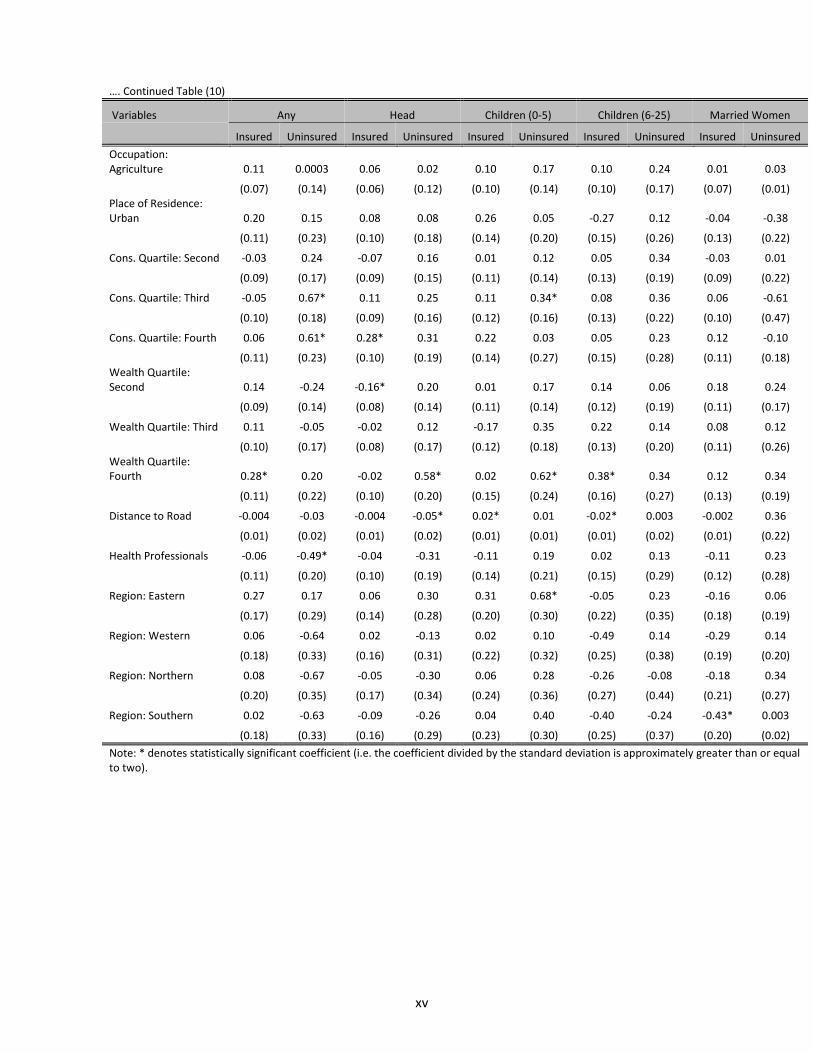
xv

…. Continued Table (10)

Variables Any Head Children (0-5) Children (6-25) Married Women

Insured Uninsured Insured Uninsured Insured Uninsured Insured Uninsured Insured Uninsured

Occupation: Agriculture 0.11 0.0003 0.06 0.02 0.10 0.17 0.10 0.24 0.01 0.03

(0.07) (0.14) (0.06) (0.12) (0.10) (0.14) (0.10) (0.17) (0.07) (0.01) Place of Residence: Urban 0.20 0.15 0.08 0.08 0.26 0.05 -0.27 0.12 -0.04 -0.38

(0.11) (0.23) (0.10) (0.18) (0.14) (0.20) (0.15) (0.26) (0.13) (0.22)

Cons. Quartile: Second -0.03 0.24 -0.07 0.16 0.01 0.12 0.05 0.34 -0.03 0.01

(0.09) (0.17) (0.09) (0.15) (0.11) (0.14) (0.13) (0.19) (0.09) (0.22)

Cons. Quartile: Third -0.05 0.67* 0.11 0.25 0.11 0.34* 0.08 0.36 0.06 -0.61

(0.10) (0.18) (0.09) (0.16) (0.12) (0.16) (0.13) (0.22) (0.10) (0.47)

Cons. Quartile: Fourth 0.06 0.61* 0.28* 0.31 0.22 0.03 0.05 0.23 0.12 -0.10

(0.11) (0.23) (0.10) (0.19) (0.14) (0.27) (0.15) (0.28) (0.11) (0.18) Wealth Quartile: Second 0.14 -0.24 -0.16* 0.20 0.01 0.17 0.14 0.06 0.18 0.24

(0.09) (0.14) (0.08) (0.14) (0.11) (0.14) (0.12) (0.19) (0.11) (0.17)

Wealth Quartile: Third 0.11 -0.05 -0.02 0.12 -0.17 0.35 0.22 0.14 0.08 0.12

(0.10) (0.17) (0.08) (0.17) (0.12) (0.18) (0.13) (0.20) (0.11) (0.26) Wealth Quartile: Fourth 0.28* 0.20 -0.02 0.58* 0.02 0.62* 0.38* 0.34 0.12 0.34

(0.11) (0.22) (0.10) (0.20) (0.15) (0.24) (0.16) (0.27) (0.13) (0.19)

Distance to Road -0.004 -0.03 -0.004 -0.05* 0.02* 0.01 -0.02* 0.003 -0.002 0.36

(0.01) (0.02) (0.01) (0.02) (0.01) (0.01) (0.01) (0.02) (0.01) (0.22)

Health Professionals -0.06 -0.49* -0.04 -0.31 -0.11 0.19 0.02 0.13 -0.11 0.23

(0.11) (0.20) (0.10) (0.19) (0.14) (0.21) (0.15) (0.29) (0.12) (0.28)

Region: Eastern 0.27 0.17 0.06 0.30 0.31 0.68* -0.05 0.23 -0.16 0.06

(0.17) (0.29) (0.14) (0.28) (0.20) (0.30) (0.22) (0.35) (0.18) (0.19)

Region: Western 0.06 -0.64 0.02 -0.13 0.02 0.10 -0.49 0.14 -0.29 0.14

(0.18) (0.33) (0.16) (0.31) (0.22) (0.32) (0.25) (0.38) (0.19) (0.20)

Region: Northern 0.08 -0.67 -0.05 -0.30 0.06 0.28 -0.26 -0.08 -0.18 0.34

(0.20) (0.35) (0.17) (0.34) (0.24) (0.36) (0.27) (0.44) (0.21) (0.27)

Region: Southern 0.02 -0.63 -0.09 -0.26 0.04 0.40 -0.40 -0.24 -0.43* 0.003

(0.18) (0.33) (0.16) (0.29) (0.23) (0.30) (0.25) (0.37) (0.20) (0.02)

Note: * denotes statistically significant coefficient (i.e. the coefficient divided by the standard deviation is approximately greater than or equal to two).

xvi

Table (11): Posterior estimates of coefficients in the potential screening services utilization under the insured and uninsured states

Variables Any Head Children (0-5) Children (6-25) Married Women

Insured Uninsured Insured Uninsured Insured Uninsured Insured Uninsured Insured Uninsured

Intercept -1.24 -1.07 -0.44 -1.74* -1.21* -3.53* -0.39 -0.34 -0.79 -0.57

(0.40) (0.91) (0.34) (0.82) (0.50) (0.93) (0.55) (1.19) (0.41) (1.25)

Household head: Male 0.15 0.16 0.07 0.26 0.11 -0.11 -0.01 -0.35

(0.12) (0.26) (0.10) (0.21) (0.15) (0.24) (0.15) (0.33)

Household head: Married -0.08 0.32 0.01 -0.16 -0.02 0.23 -0.06 0.39

(0.10) (0.21) (0.10) (0.20) (0.11) (0.18) (0.14) (0.30)

Household head: Age 0.002 -0.02* -0.004* -0.01 0.01* 0.004 -0.004 -0.02*

(0.00) (0.01) (0.00) (0.01) (0.00) (0.01) (0.00) (0.01)

No. of children aged 0-5 -0.01 -0.06 -0.03 -0.04 0.11 -0.05 -0.02 -0.06 0.03 0.10

(0.05) (0.12) (0.04) (0.10) (0.07) (0.12) (0.07) (0.14) (0.04) (0.14)

No. of children aged 6-25 -0.04 0.01 -0.003 0.005 -0.01 0.09 -0.01 0.13 -0.02 0.09

(0.03) (0.07) (0.02) (0.05) (0.03) (0.05) (0.04) (0.10) (0.02) (0.07)

Male -0.15 -0.38 -0.06 0.16 -0.03 -0.36

(0.09) (0.20) (0.08) (0.14) (0.10) (0.24)

Age -0.01* -0.01 -0.05 -0.12* -0.003 0.02 -0.005 -0.03*

(0.00) (0.01) (0.03) (0.05) (0.01) (0.02) (0.00) (0.01)

Relation to the Head: Spouse 0.05 -0.42

(0.13) (0.34)

Relation to the Head: BioChild -0.11 -0.04 0.06 0.37 -0.13 -0.31

(0.16) (0.36) (0.16) (0.29) (0.14) (0.35)

Relation to the Head: Other 0.05 -0.12

(0.20) (0.45)

Education: Primary 0.17 -0.07 0.08 0.38 0.13 -0.07 0.01 0.28 -0.03 -0.05

(0.11) (0.27) (0.09) (0.26) (0.13) (0.24) (0.15) (0.33) (0.11) (0.33)

Education: Second/University 0.32 -0.10 0.19 0.50 0.32 0.49 -0.08 0.16 -0.06 0.40

(0.19) (0.52) (0.17) (0.48) (0.19) (0.40) (0.22) (0.58) (0.19) (0.70)

Education: Vocational 0.07 0.09 0.05 0.25 0.09 -0.02 0.003 0.07 -0.05 0.08

(0.09) (0.21) (0.08) (0.21) (0.11) (0.19) (0.12) (0.29) (0.09) (0.30)

Note: * denotes statistically significant coefficient (i.e. the coefficient divided by the standard deviation is approximately greater than or equal to two).

… Table (11) continued

xvii

… Continued Table (11)

Variables Any Head Children (0-5) Children (6-25) Married Women

Insured Uninsured Insured Uninsured Insured Uninsured Insured Uninsured Insured Uninsured

Occupation: Agriculture 0.02 0.25 0.03 -0.01 0.14 0.62* -0.03 -0.17 0.02 -0.49

(0.08) (0.21) (0.07) (0.18) (0.09) (0.20) (0.11) (0.24) (0.08) (0.27) Place of Residence: Urban 0.19 0.48 0.21 0.64* 0.05 0.45 -0.05 0.60 0.05 -0.26

(0.12) (0.30) (0.11) (0.22) (0.16) (0.25) (0.17) (0.35) (0.14) (0.43) Cons. Quartile: Second -0.05 0.29 -0.12 0.09 -0.003 -0.03 0.02 0.23 -0.03 0.26

(0.11) (0.27) (0.10) (0.22) (0.12) (0.20) (0.15) (0.30) (0.10) (0.29)

Cons. Quartile: Third 0.01 0.76* 0.02 0.20 0.03 0.46* 0.12 0.28 0.03 0.28

(0.11) (0.25) (0.10) (0.22) (0.12) (0.22) (0.15) (0.33) (0.11) (0.33) Cons. Quartile: Fourth 0.04 0.60 0.17 0.19 0.08 0.58 0.24 0.73 0.13 0.75

(0.13) (0.33) (0.11) (0.27) (0.14) (0.32) (0.17) (0.40) (0.12) (0.43) Wealth Quartile: Second 0.08 -0.42 -0.16 -0.18 0.14 0.08 -0.001 0.02 0.12 -0.40

(0.11) (0.24) (0.09) (0.21) (0.12) (0.18) (0.14) (0.27) (0.12) (0.26) Wealth Quartile: Third 0.14 0.10 -0.06 0.06 0.05 0.36 0.18 -0.75 0.04 -0.94*

(0.11) (0.23) (0.09) (0.23) (0.13) (0.23) (0.15) (0.38) (0.12) (0.38) Wealth Quartile: Fourth 0.17 0.37 -0.06 0.25 0.08 0.39 0.19 -0.38 0.09 -0.11

(0.13) (0.32) (0.11) (0.28) (0.16) (0.32) (0.18) (0.38) (0.13) (0.39)

Distance to Road 0.03 0.0002 0.004 -0.02 0.02 0.01 -0.01 0.07 0.0000 -0.02

(0.01) (0.02) (0.01) (0.02) (0.01) (0.02) (0.01) (0.03) (0.01) (0.03)

Health Professionals 0.08 -0.28 -0.11 -0.33 0.02 0.20 0.01 -0.42 0.14 0.04

(0.13) (0.32) (0.11) (0.28) (0.14) (0.27) (0.17) (0.40) (0.13) (0.37)

Region: Eastern 0.29 0.38 0.05 1.02 0.13 0.88* 0.08 -0.23 0.07 0.72

(0.18) (0.45) (0.16) (0.44) (0.21) (0.44) (0.24) (0.48) (0.20) (0.55)

Region: Western 0.17 -0.10 -0.07 0.63 -0.15 0.03 -0.28 -0.38 0.09 -0.63

(0.20) (0.46) (0.17) (0.47) (0.23) (0.48) (0.27) (0.56) (0.21) (0.77)

Region: Northern 0.16 -0.41 -0.23 0.43 -0.08 -0.24 -0.29 -0.44 0.10 0.34

(0.22) (0.53) (0.19) (0.54) (0.24) (0.60) (0.29) (0.63) (0.23) (0.70)

Region: Southern 0.14 -0.13 -0.13 0.50 -0.12 0.71 -0.16 -0.95 -0.05 0.16

(0.20) (0.47) (0.18) (0.47) (0.23) (0.45) (0.26) (0.56) (0.23) (0.60)

Note: * denotes statistically significant coefficient (i.e. the coefficient divided by the standard deviation is approximately greater than or equal to two).

xviii

Table (12): Posterior estimates of coefficients in the potential drug utilization under the insured and uninsured states

Variables Any Head Children (0-5) Children (6-25) Married Women

Insured Uninsured Insured Uninsured Insured Uninsured Insured Uninsured Insured Uninsured

Intercept -0.82* -1.14* -0.50 -1.14* -0.55 -0.93 -0.39 -1.86* 0.04 -1.12

(0.36) (0.53) (0.31) (0.53) (0.49) (0.59) (0.52) (0.74) (0.37) (0.69)

Household head: Male -0.02 -0.03 0.01 -0.03 -0.03 -0.06 0.07 0.15

(0.11) (0.15) (0.09) (0.15) (0.14) (0.16) (0.14) (0.19)

Household head: Married 0.06 -0.02 0.08 -0.02 -0.08 0.06 -0.16 -0.09

(0.09) (0.13) (0.09) (0.13) (0.10) (0.13) (0.13) (0.18)

Household head: Age 0.001 -0.002 -0.003 -0.002 0.01* -0.003 -0.001 -0.01*

(0.001) (0.01) (0.001) (0.01) (0.0001) (0.01) (0.001) (0.001)

No. of children aged 0-5 0.03 0.01 0.06 0.01 -0.01 -0.07 0.06 0.03 0.01 -0.01

(0.04) (0.07) (0.04) (0.07) (0.07) (0.08) (0.06) (0.08) (0.04) (0.07)

No. of children aged 6-25 -0.02 0.03 -0.02 0.03 -0.02 0.06* 0.04 -0.01 0.001 0.03

(0.02) (0.04) (0.02) (0.04) (0.03) (0.03) (0.04) (0.05) (0.02) (0.04)

Male -0.01 0.09 -0.01 0.17 0.09 0.18

(0.08) (0.12) (0.08) (0.10) (0.09) (0.13)

Age -0.003 -0.01 -0.09* -0.08* 0.004 0.02* -0.004* -0.01*

(0.00) (0.01) (0.03) (0.03) (0.01) (0.01) (0.0001) (0.0001)

Relation to the Head: Spouse 0.04 0.35

(0.11) (0.18) Relation to the Head: Biological Child 0.01 0.13 0.29 0.18 -0.10 -0.10

(0.15) (0.23) (0.15) (0.19) (0.13) (0.19)

Relation to the Head: Other 0.02 -0.21

(0.19) (0.29)

Education: Primary 0.30* -0.11 0.16* 0.09 0.33* -0.13 0.12 0.09 0.18 0.01

(0.10) (0.16) (0.08) (0.12) (0.12) (0.16) (0.13) (0.19) (0.10) (0.16) Education: Second/University 0.45* -0.18 0.31* -0.01 0.38 0.70 0.06 -0.13 0.17 0.26

(0.18) (0.33) (0.15) (0.01) (0.20) (0.36) (0.21) (0.41) (0.18) (0.42)

Education: Vocational 0.13 0.01 0.03 0.35 0.24* 0.005 0.02 0.03 0.01 0.05

(0.08) (0.11) (0.07) (0.18) (0.11) (0.13) (0.11) (0.15) (0.08) (0.14)

Note: * denotes statistically significant coefficient (i.e. the coefficient divided by the standard deviation is approximately greater than or equal to two).

… Table (12) continued

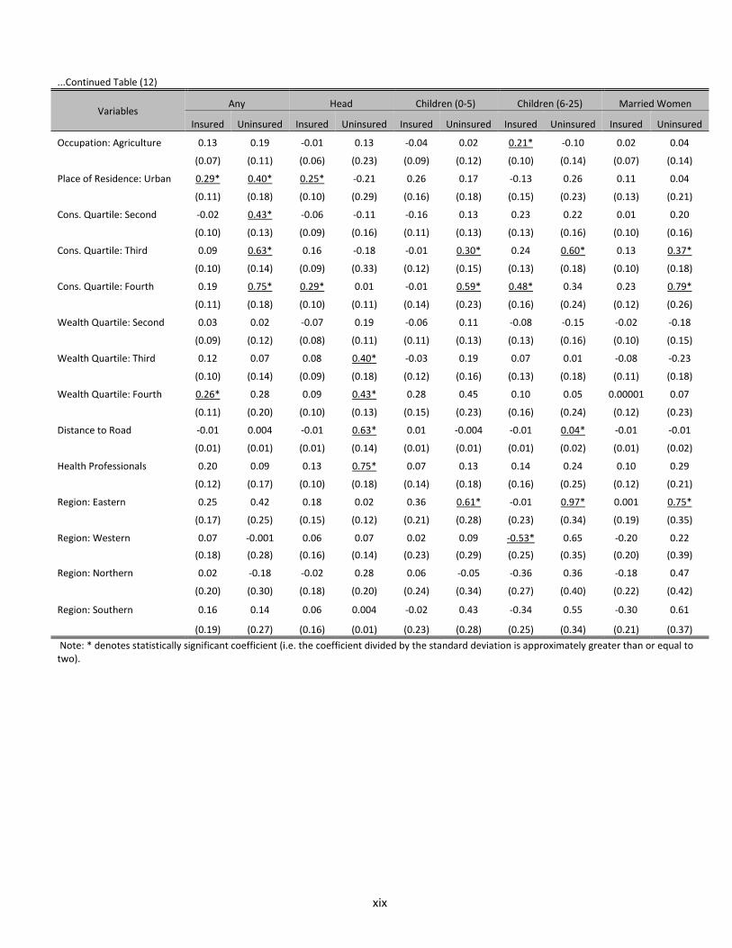
xix

...Continued Table (12)

Variables Any Head Children (0-5) Children (6-25) Married Women

Insured Uninsured Insured Uninsured Insured Uninsured Insured Uninsured Insured Uninsured

Occupation: Agriculture 0.13 0.19 -0.01 0.13 -0.04 0.02 0.21* -0.10 0.02 0.04

(0.07) (0.11) (0.06) (0.23) (0.09) (0.12) (0.10) (0.14) (0.07) (0.14)

Place of Residence: Urban 0.29* 0.40* 0.25* -0.21 0.26 0.17 -0.13 0.26 0.11 0.04

(0.11) (0.18) (0.10) (0.29) (0.16) (0.18) (0.15) (0.23) (0.13) (0.21)

Cons. Quartile: Second -0.02 0.43* -0.06 -0.11 -0.16 0.13 0.23 0.22 0.01 0.20

(0.10) (0.13) (0.09) (0.16) (0.11) (0.13) (0.13) (0.16) (0.10) (0.16)

Cons. Quartile: Third 0.09 0.63* 0.16 -0.18 -0.01 0.30* 0.24 0.60* 0.13 0.37*

(0.10) (0.14) (0.09) (0.33) (0.12) (0.15) (0.13) (0.18) (0.10) (0.18)

Cons. Quartile: Fourth 0.19 0.75* 0.29* 0.01 -0.01 0.59* 0.48* 0.34 0.23 0.79*

(0.11) (0.18) (0.10) (0.11) (0.14) (0.23) (0.16) (0.24) (0.12) (0.26)

Wealth Quartile: Second 0.03 0.02 -0.07 0.19 -0.06 0.11 -0.08 -0.15 -0.02 -0.18

(0.09) (0.12) (0.08) (0.11) (0.11) (0.13) (0.13) (0.16) (0.10) (0.15)

Wealth Quartile: Third 0.12 0.07 0.08 0.40* -0.03 0.19 0.07 0.01 -0.08 -0.23

(0.10) (0.14) (0.09) (0.18) (0.12) (0.16) (0.13) (0.18) (0.11) (0.18)

Wealth Quartile: Fourth 0.26* 0.28 0.09 0.43* 0.28 0.45 0.10 0.05 0.00001 0.07

(0.11) (0.20) (0.10) (0.13) (0.15) (0.23) (0.16) (0.24) (0.12) (0.23)

Distance to Road -0.01 0.004 -0.01 0.63* 0.01 -0.004 -0.01 0.04* -0.01 -0.01

(0.01) (0.01) (0.01) (0.14) (0.01) (0.01) (0.01) (0.02) (0.01) (0.02)

Health Professionals 0.20 0.09 0.13 0.75* 0.07 0.13 0.14 0.24 0.10 0.29

(0.12) (0.17) (0.10) (0.18) (0.14) (0.18) (0.16) (0.25) (0.12) (0.21)

Region: Eastern 0.25 0.42 0.18 0.02 0.36 0.61* -0.01 0.97* 0.001 0.75*

(0.17) (0.25) (0.15) (0.12) (0.21) (0.28) (0.23) (0.34) (0.19) (0.35)

Region: Western 0.07 -0.001 0.06 0.07 0.02 0.09 -0.53* 0.65 -0.20 0.22

(0.18) (0.28) (0.16) (0.14) (0.23) (0.29) (0.25) (0.35) (0.20) (0.39)

Region: Northern 0.02 -0.18 -0.02 0.28 0.06 -0.05 -0.36 0.36 -0.18 0.47

(0.20) (0.30) (0.18) (0.20) (0.24) (0.34) (0.27) (0.40) (0.22) (0.42)

Region: Southern 0.16 0.14 0.06 0.004 -0.02 0.43 -0.34 0.55 -0.30 0.61

(0.19) (0.27) (0.16) (0.01) (0.23) (0.28) (0.25) (0.34) (0.21) (0.37)

Note: * denotes statistically significant coefficient (i.e. the coefficient divided by the standard deviation is approximately greater than or equal to two).

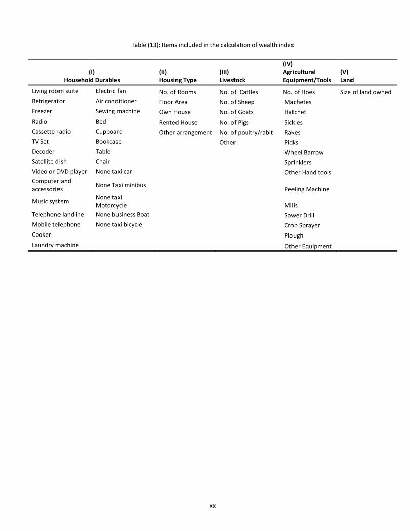
xx

Table (13): Items included in the calculation of wealth index

(I) Household Durables

(II) Housing Type

(III) Livestock

(IV) Agricultural Equipment/Tools

(V) Land

Living room suite Electric fan No. of Rooms No. of Cattles No. of Hoes Size of land owned

Refrigerator Air conditioner Floor Area No. of Sheep Machetes

Freezer Sewing machine Own House No. of Goats Hatchet

Radio Bed Rented House No. of Pigs Sickles

Cassette radio Cupboard Other arrangement No. of poultry/rabit Rakes

TV Set Bookcase Other Picks

Decoder Table Wheel Barrow

Satellite dish Chair Sprinklers

Video or DVD player None taxi car Other Hand tools Computer and accessories

None Taxi minibus Peeling Machine

Music system None taxi Motorcycle Mills

Telephone landline None business Boat Sower Drill

Mobile telephone None taxi bicycle Crop Sprayer

Cooker Plough

Laundry machine Other Equipment

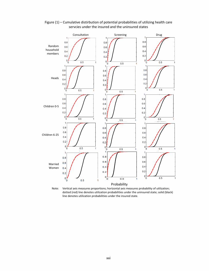
xxi

Figure (1) – Cumulative distirbution of potential probabilities of utilizing health care servcies under the insured and the uninsured states

Consultation

Screening

Drug

Random household members

Heads

Children 0-5

Children 6-25

Married Women

Probability Note: Vertical axis measures proportions; horizontal axis measures probability of utilization;

dotted (red) line denotes utilization probabilities under the uninsured state; solid (black) line denotes utilization probabilities under the insured state.

xxii

Figure (2a) – Histogram of Individual-Level Treatment Effects

Consultation

Screening

Drug

Random household members

Heads

Children 0-5

Children 6-25

Married women

Treatment Effects

xxiii

Figure (2b) – Bar plot of ATEs by district and healthcare services

0.00 0.10 0.20 0.30 0.40 0.50 0.60 0.70 0.80

Ngoma

Kirehe

Nyagatare

Bugesera

Gatsibo

Gasabo

Rwamagana

Nyarugenge

Kamonyi

Nyabihu

Kayonza

Nyaruguru

Rubavu

Rutsiro

Rusizi

Gisagara

Muhanga

Musanze

Burera

Ruhango

Rulindo

Ngororero

Nyamasheke

Gicumbi

Huye

Nyanza

Nyamagabe

Kicukiro

Gakenke

KarongiD

istr

ict Consultation

Screening

Drugs

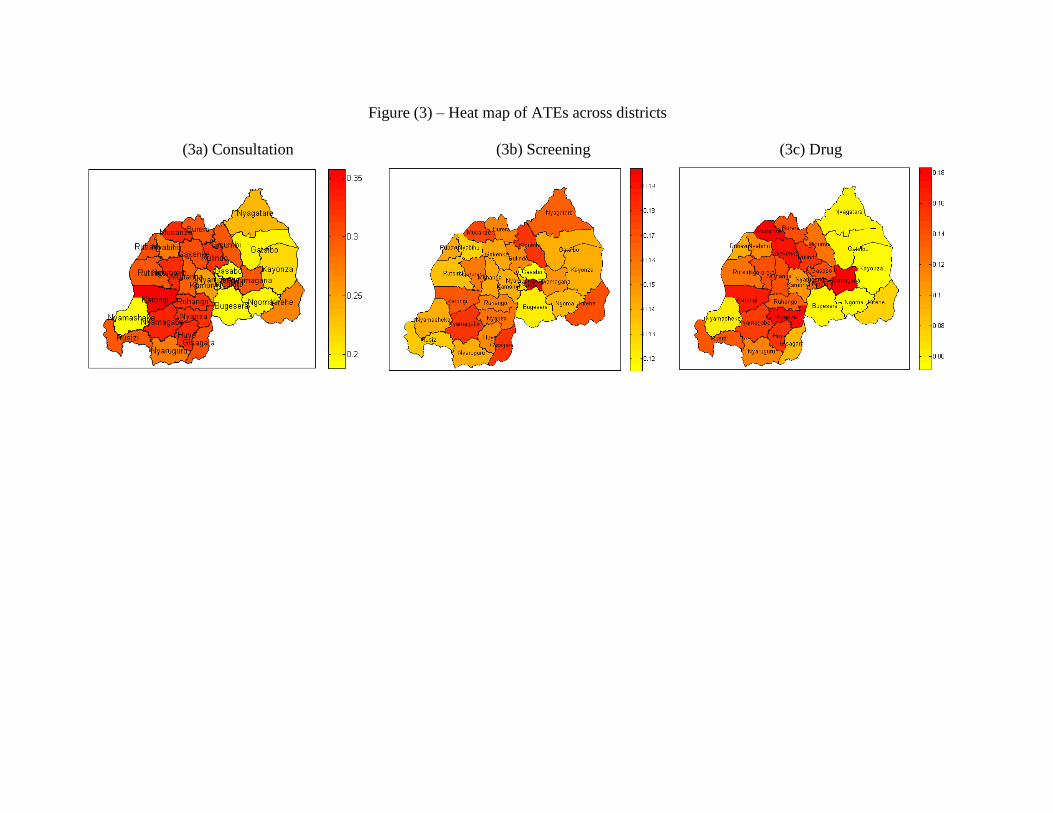
Figure (3) – Heat map of ATEs across districts

(3a) Consultation (3b) Screening (3c) Drug

Recent Publications in the Series

nº Year Author(s) Title

224 2015 Gibert Galibaka

Sophistication of Fruits , Vegetables and Derivatives Exports in the WAEMU space

223 2015 Zorobabel Bicaba, Zuzana Brixiová

and Mthuli Ncube

Extreme Poverty in Africa: Trends, Policies and the Role

of International Organizations

222 2015 Anthony M. Simpasa, Abebe

Shimeles and Adeleke O. Salami

Employment Effects of Multilateral Development

BankSuport: The Case of the African Development Bank

221 2015 Ousman Gajigo and Mouna Ben

Dhaou Economies of Scale in Gold Mining

220 2015 Zerihun Gudeta Alemu Developing a Food (in) Security Map for South Africa

219 2015 El-hadj Bah Impact of the Business Environment on Output and

Productivity in Africa

218 2015 Nadege Yameogo Household Energy Demand and the Impact of Energy

Prices: Evidence from Senegal

217 2015 Zorobabel Bicaba, Zuzana Brixiová,

and Mthuli Ncube

Capital Account Policies, IMF Programs and Growth in

Developing Regions

216 2015 Wolassa L Kumo Inflation Targeting Monetary Policy, Inflation Volatility

and Economic Growth in South Africa

215 2014 Taoufik Rajhi A Regional Budget Development Allocation Formula for

Tunisia