A FRAMEWORK FOR MEASURING SUPERCOMPUTER PRODUCTIVITY1

10/30/2003

Marc Snir2 and David A. Bader3

Abstract We propose a framework for measuring the productivity of High Performance Computing (HPC) systems, based on common economic definitions of productivity and on Utility Theory. We discuss how these definitions can capture essential aspects of HPC systems, such as the importance of time-to-solution and the trade-off between programming time and execution time. Finally, we outline a research program that would lead to the definition of effective productivity metrics for HPC that fit within the proposed framework.

1. Introduction

Productivity is an important subject of economic study, for obvious reasons: At the microeconomic level, an increase in productivity results in an increase in firm profits. At the macroeconomic level, an increase in productivity boosts the Gross Domestic Product. An important concern is to ensure that productivity is properly measured, as improper measures will lead to suboptimal investment and policy decisions, at the micro and the macro level.

The recent DARPA High-Productivity Computing Systems initiative [2] has raised the issue of proper productivity measurements, in the context of high-performance computing (HPC). The motivation is the same as in the general economic realm: Proper productivity measures will lead to better investments and better policy decisions in HPC. The HPC world has been obsessively focused on simple performance metrics, such as peak floating-point performance, or performance on the Linpack benchmark [6]. It would seem that these performance measures have often been used as proxies for total productivity measures, resulting in gross distortions in investment decisions.

This paper proposes a framework for measuring the productivity of HPC systems. The basic framework is introduced in Section 2 and is discussed in Section 3. A possible approach for defining productivity metrics is introduced and discussed in Section 4. We conclude with a brief discussion.

2. Basics

Productivity is usually defined, in Economics, as the amount of output per unit of input. Thus, the labor productivity of workers in the car industry can be measured as the number

1 This work is supported in part by DARPA Contract NBCHC-02-0056 and NBCH30390004. 2 Computer Science, University of Illinois at Urbana Champaign. Also supported in part by DOE Grant DE-

FG02-03ER25560. 3 Electrical and Computer Engineering, University of New Mexico, Albuquerque. Also supported in part by NSF

Grants CAREER ACI-00-93039, ITR EIA-01-21377, Biocomplexity DEB-01-20709, and ITR EF/BIO 03-31654.

1

of cars produced per work hour (or, inversely, as the number of work hours needed to produce a car); the labor productivity of the US economy is measured as the ratio between the Gross Domestic Product and worker hours in the US. In this definition, one input measure (hours worked) is compared to one output measure (cars produced or GDP).

It is important to realize, in the first example, that the productivity of the car workers depends not only on their skills or motivation but also on the equipment available in car factories, and on the type of cars manufactured. By the measure of work hours per car, workers in a heavily automated (more capital intensive) plant are likely to be more productive than workers in a less automated (less capital intensive) plant; and workers that produce Rolls-Royce cars are likely to be less productive than workers that produce Saturn cars, if productivity is measured in number of cars.

The last bias can be avoided, to a large extent, if instead of counting car units one counts units of car value, i.e. the monetary value of cars produced in one work hour. In some contexts it may be useful to also measure the units of input in terms of their cost – e.g., by counting salary expenses, rather than hours of work. This is especially important for inputs that are heterogeneous and have no obvious common measure. If we do so, then productivity becomes a unit-less measure, namely the ratio between value produced and value of one of the inputs consumed to produce this value.

In some cases, it is useful to consider more than one input. Total productivity measures attempt to consider the sum of all inputs together. In order to obtain a meaningful measure, the various inputs need to be properly weighted. One obvious choice is to weight them by their cost, in which case productivity becomes the ratio between the units of output (or value of output) and cost of inputs.

The same approach can be used to measure the productivity of a factor or a set of factors: e.g., the productivity of a car plant, the productivity of a production line, the productivity of IT in the car industry, etc.

Suppose that we are to apply the same approach to define the productivity of supercomputing systems. The productivity of a supercomputer would be defined as the total units of output produced by this system, divided by its cost. We are faced with an immediate problem: how do we measure the output of a supercomputer? Clearly, simple measures such as number of operations performed, or number of jobs run will not do. As we do not have an efficient market for supercomputing results, we cannot use output market value, either.

Utility Theory, as axiomatized by von Neumann and Morgenstern [20, 35], provides a way out. Utility theory is an attempt to infer subjective value, or utility, from choices. Utility theory can be used in decision making under risk or uncertainty. Utility theory can be assumed to be descriptive, i.e. used to describe how people make choices. Alternatively, it can be assumed to be prescriptive or normative, i.e. used to describe how people should make choices under a rational model of decision making. This paper espouses this latter view.

Formally, one assumes a set X of outcomes and a relation f that expresses preferences of some rational agent over outcomes or lotteries of outcomes. A lottery is a finite subset of outcomes 1{ , , }kx x ⊂K X k, with associated probabilities 1, ,p pK ; 1ip =∑ . We denote

2

by the set of lotteries over outcomes in ( )X∆ X . Note that ( )X∆ is a convex set: if , ( )x y X∈∆ are lotteries, and 0 1α≤ ≤ , then (1 )x yα α+ − is a lottery in . ( )X∆

The preference relation is assumed to fulfill the following axioms.

1. is complete, i.e. either f x yf or for ally xf , ( )x y X∈∆ .

2. is transitive, i.e. if f x yf and , then y zf x zf for all , , ( )x y z X∈∆ .

3. Archimedean axiom: if x y zf f then there exist α andβ , 0 1α β< < < , such that (1 )y x zα α+ −f and (1 )x z yβ β+ − f . This is a weak continuity axiom for lotteries.

4. Independence Axiom: x yf if and only if (1 ) (1 )x z y zα α α α+ − + −f . This axiom asserts that preferences between x and are unaffected if we combine both with another outcome in the same way.

y

These axioms are satisfied if and only if there is a real-valued utility function U such that

1. U represents ; i.e.f , ( ), ( ) ( )x y x x y U x U∀ ∈∆ ⇒ >f y .

2. U is affine; i.e. , ( ), [0,1], ( (1 ) ) ( ) (1 ) ( ).x y X U x y U x U yα α α α α∀ ∈∆ ∈ + − = + −

Furthermore, U is unique, up to positive linear transformations. Thus, if “rational” preferences are expected to satisfy the four listed axioms, then any system of rational preferences can be represented by a utility function. The utility function is unit-less.

The utility function that represents the preferences of an agent can be estimated indirectly by assessing these preferences, e.g., by offering the agent a series of hypothetical choices. Clearly, this approach may not be very practical in an environment where there are multiple, complex outcomes. However, many of the results in this paper do not depend on the exact shape of the utility function.

One assumes that the total value of a supercomputer’s output is defined by the (rational) preference of some agent (e.g., a lab director, or a program manager). The agent’s preference can be represented by a utility function. We can now use the utility produced by the supercomputer as a measure of its output.

We shall define the productivity of a supercomputer system as the ratio between the utility of the output it computes to the cost of the system. This measure depends on the preferences of an agent, rather than being objectively defined. This is unavoidable: The value of the output of a supercomputer may vary from organization to organization; as long as there is no practical way to trade supercomputer outputs, there is no way to directly compare the worth of a supercomputer for one organization to the worth of a supercomputer for another organization. (An indirect comparison can be made by ascertaining how much an organization is willing to pay for the machine.) In any case, much of what we shall say in this paper is fairly independent on the exact shape of the utility function. The units of productivity are utility divided by a monetary unit such as dollars.

The definition allows for some flexibility in the definition of a “system”. This may include the machine only; or it may include all the expenses incurred in using the system,

3

including capital and recurring cost for the building that hosts it, maintenance, software costs, etc. One definition is not intrinsically better than the other: The first definition makes sense when the only choice considered is whether to purchase a piece of hardware. The second definition makes sense when one considers long term choices.

If one wishes to account for all costs involved in the use of a system, then once faces a cost allocation problem: many of the expenses incurred (such as replacement cost of the capital investment in a machine room) may be shared by several systems. It is not always straightforward to properly allocate a fraction of the cost to each system. Various solutions have been proposed to this problem; see, e.g., [36]. This issue of cost evaluation and cost allocation may be non–trivial, but is a standard accounting problem that occurs in the same form at any firm that uses information technology, and is addressed by many accounting textbooks. We shall not further pursue this matter.

To the same extent that we can extend the definition of what a “system” is, we can restrict it to include only the resources made available to one application. Here, again, we face the problem of proper cost allocation (or of proper resource pricing), which we do not address in this paper.

The utility of an output is a function of its timeliness. A simulation that predicts the weather for Wednesday November 5th 2003 is valuable if completed on Tuesday November 4th, or earlier; it is most likely worthless if completed on Thursday November 6th. Thus, the utility of an output depends not only on what is computed, but also on when the computation is done. Completion time is part of the output definition, and is an argument that influences utility.

Our discussion will focus on time-to-solution as a variable parameter that affects the utility of an output. The result of a computation may have other parameters that affect its utility, such as its accuracy, or its trustworthiness (i.e., the likelihood that the code used is a correct implementation of the algorithm it is supposed to embody). In some situations, time-to-solution may be fixed, but other parameters can be varied. Thus, one may fix the period of time dedicated to a weather simulation, but vary the accuracy of the simulation (grid resolution, accuracy of physics representation, number of scenarios simulated, etc.). The general framework can accommodate such variants.

3. Discussion of Basic Framework

To simplify discussion, we consider in this section an idealized situation where a system S will be purchased uniquely to develop from scratch and solve once a problem P. By “system”, we mean the programming environment that is used to develop the code and the (hardware and software) system that is used to run it. There are multiple possible choices of systems to purchase, programming language to use for implementing the application, programming efforts to invest in coding and tuning the application, etc. What is the rationale for such choices?

We study the problem by assuming three independent variables; namely T, the time-to-solution, S, the system used, and U, the utility function that represents preferences on outcomes. Thus, given, S and T, we minimize the cost of solving problem P on system S in

4

time T. We denote the (minimal) cost of such a solution by Each time-to-solution T is associated with a utility

( , , ).C P S T( , )U U P T= and a productivity

( , )( , , , ) .

( , , )U P TP S T U

C P S TΨ =

Then, the ideal productivity of system S for problem P is defined to be

( , )( , , ) max ( , , , ) max

( , , )T TU P TP S U P S T U

C P S TΨ = Ψ =

( , , ( , ))P S UΨ = Ψ ⋅ ⋅ is the (best possible) productivity for problem P on system S, relative to utility function Note that productivity normally indicates a measured ratio of outputs to inputs, in a given environment; ideal productivity is a measure of productivity that can be potentially obtained, assuming optimal decisions.

( , ).U U P T=

Our ultimate purpose is to be able to compare the “value” of vendor systems. We say that system is better than system for problem P with respect to utility function U if

. 1S 2S

1 2( , , ( , )) ( , , ( , ))P S U P S UΨ ⋅ ⋅ > Ψ ⋅ ⋅

The formalism of this section reflects two obvious observations:

1. The ideal productivity of a system depends on the type of application that is run on this system; a collection of networked PCs may be the most productive system to look for evidence of extra-terrestrial intelligence (especially when the compute time is freely donated) [12], but may not be very productive for simulating nuclear explosions [1]. For some applications, the ideal productivity is an open question; for example, protein folding using idle cycle-stealing from networked PC’s (e.g., Stanford’s Folding@Home project [30]) versus using innovative architectures (e.g., the IBM BlueGene project [11]).

2. The productivity of a system depends on the time sensitivity of the result that is represented by the utility function U. If the result is as valuable if obtained twenty years from now as if obtained in a week, then there is no reason to buy an expensive supercomputer; one can just wait until the computation fits on a PC (or a game machine). On the other hand, if it is very important to complete the computation in a week, then an expensive high-end machine and a quick prototyping programming environment may prove the more productive system.

We can use the same approach to compare other alternatives, by suitably redefining what we mean by a “system”. For example, assume that we want to compare two programming environments that are both supported on a vendor system, in order to decide which should be used to solve problem P: Define to be the system with the first programming environment and to be the system with the second programming environment, and proceed as before.

1S

2S

We proceed now to discuss more in detail costs and utilities.

5

3.1. Utility

time

ytilitU

Figure 1: Utility decreases with time

Utility U P is a decreasing function of time-to-solution T, as illustrated in Figure 1, because there is no loss in acquiring information earlier (information does not deteriorate),

and there may be some benefit. (A possible counterexample is a situation where the cost of storing the output of a computation until it can be acted upon is high. However, in cases of interest to us, the cost of storing the result of a computation is insignificant compared to the cost of the computation itself.) In many environments, the value of a solution may steeply decline over time: intelligence quickly loses its value; weather must be simulated accurately in time to provide a prediction, etc.

At the other extreme, fundamental research is relatively time insensitive, so that value declines

moderately with time. This motivates two value-time curves. A deadline driven utility is defined by

( , )

6

Time

ytilitU

Figure 2: Deadline-driven utility

T

( , )U P T u=

if( , )

0 ifu T deadline

U P TT deadline≤⎧

= ⎨ >⎩ (1)

This yields the step-function curve illustrated in Figure 2. The curve illustrated in Figure 3 corresponds to fixed, time independent utility; i.e.,

(2)

The curve in Figure 4 illustrates a staircase function that approximates a commonly occurring situation in industry, or in national labs (see, e.g., [27]): The highest utility is associated with “near-interactive time” computations; i.e., a computation that take less than a coffee-break so that it can be part of

an uninterrupted engineering development cycle. Above a certain time, computations tend to be postponed to overnight runs, so the next level represents the utility of a computation done overnight, that can be part of a daily development cycle. The third threshold corresponds to the utility of computations that cannot be done overnight, and which tend to be done “once in a project lifetime”.

Time

ytilitU

Figure 3: Time independent utility 3.2. Cost

Cost can be decomposed into development

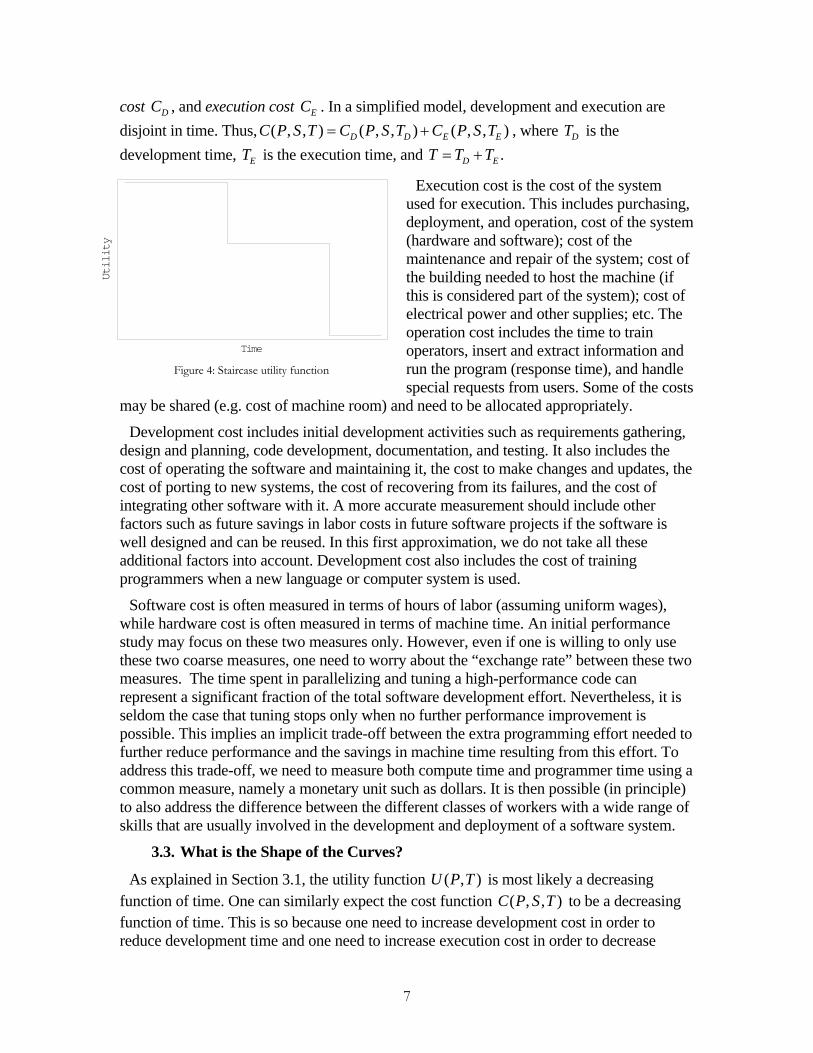
cost DC , and execution cost . In a simplified model, development and execution are disjoint in time. Thus,

EC( , , ) ( , , ) ( , , )D D E EC P S T C P S T C P S T= + , where DT is the

development time, is the execution time, and ET .D ET T T= +

Execution cost is the cost of the system used for execution. This includes purchasing, deployment, and operation, cost of the s(hardware and software); cost of the maintenance and repair of the system; cost of the building needed to host the machine (if this is considered part of the system); cost of electrical power and other supplies; etc. The operation cost includes the time to train operators, insert and extract information and run the program (response time), and handle special requests from users. Some of the c

may be shared (e.g. cost of machine room) and need to be allocated appropriately.

Time

ytilitU

ystem

osts Figure 4: Staircase utility function

Development cost includes initial development activities such as requirements gathering, design and planning, code development, documentation, and testing. It also includes the cost of operating the software and maintaining it, the cost to make changes and updates, the cost of porting to new systems, the cost of recovering from its failures, and the cost of integrating other software with it. A more accurate measurement should include other factors such as future savings in labor costs in future software projects if the software is well designed and can be reused. In this first approximation, we do not take all these additional factors into account. Development cost also includes the cost of training programmers when a new language or computer system is used.

Software cost is often measured in terms of hours of labor (assuming uniform wages), while hardware cost is often measured in terms of machine time. An initial performance study may focus on these two measures only. However, even if one is willing to only use these two coarse measures, one need to worry about the “exchange rate” between these two measures. The time spent in parallelizing and tuning a high-performance code can represent a significant fraction of the total software development effort. Nevertheless, it is seldom the case that tuning stops only when no further performance improvement is possible. This implies an implicit trade-off between the extra programming effort needed to further reduce performance and the savings in machine time resulting from this effort. To address this trade-off, we need to measure both compute time and programmer time using a common measure, namely a monetary unit such as dollars. It is then possible (in principle) to also address the difference between the different classes of workers with a wide range of skills that are usually involved in the development and deployment of a software system.

3.3. What is the Shape of the Curves?

As explained in Section 3.1, the utility function is most likely a decreasing function of time. One can similarly expect the cost function to be a decreasing function of time. This is so because one need to increase development cost in order to reduce development time and one need to increase execution cost in order to decrease

( , )U P T( , , )C P S T

7

execution time. In order to reduce development time, one may increase the number of programmers. But an increase in the number of programmers assigned to a programming task does not usually result in a proportional decrease in development time [18]. Similarly, in order to reduce execution cost, one may use a machine with more processors. But speedup is seldom linear in the number of processors. Thus, stretching the time-to-solution reduces cost (up to a point) but also reduces the utility of the result.

By composing the cost-time curve and the utility-time curve one obtains a productivity-time curve: ( , , , ) ( , ) / ( , , )P S T U U P T C P S TΨ = . Little can be said, a-priori, about its shape: it depends on how fast cost decreases when one stretches time-to-solution versus how fast the utility of the result decreases. In many cases we expect a unimodal curve as illustrated in Figure 5, with one optimal solution that gives us the ideal (optimal) productivity. At one end, if we stretch development time beyond the bare minimum possible then productivity increases,

since the marginal cost for a reduction in time-to-solution is very steep, when we get close to the minimum. At the other end, if we stretch time-to-solution too much then productivity decreases, since there are almost no further cost savings, while utility continues to drop.

Time

ytivitcudorP

Figure 5: Productivity as a function of time-to-solution

Consider the two extremes:

Flat utility-time curve (Equation (2)). Productivity is inversely proportional to cost, and, hence is monotonically increasing:

( , )( , , , ) .

( , , ) ( , , )U P T uP S T U

C P S T C P S TΨ = =

If utility does not decrease over time, then the development and execution process with the slowest practical progress rate, which is the cheapest, will also be the most productive. There is no reason to ever use a parallel machine, or to have more than one application developer working on a project, if time is not an issue. Parallelism increases some costs in order to reduce time to solution. Its use is premised on the assumption of decreasing utility with time. This clearly indicates why one must take into account the fact that utility decreases over time.

Deadline-driven utility-time curve (Equation (1)). Productivity is inversely proportional immediately drops to zero:

deadline, , ) ifS T T ≤

to cost and increases, up to the deadline, then

( , , , )0 if

u C PP S T U

T⎧

Ψ = ⎨ >⎩

deadline/ (

8

Since cost is monotonically decreasing, onobtains a curve as illustrated in Figure 6. In this case, the most productive solution is thone that accelerates time to s

e

e olution so as to

meet the deadline, but no more. This ignores uncertainty and risk. In practice, uncertainty

of

The discussion of the last sections assumed time T to be the fre meter, and cost C to be the dependent parameter. That is, one sets time to solution, and spends the amount

9

on the time needed to solve the problem will lead to a solution that provides a margin safety from the deadline. We shall further revisit this issue in Section 3.5.

3.4. Duality

Time

ytivitcudorP

Figure 6: Productivity for deadline-driven utility function

e para

needed in order to achieve that deadline. Instead, one can set budget, and look at time to solution as dependent on budget. We define, accordingly, ( , , )T P S C to be the minimal time needed to solve problem P on system S with cost C. It is easy to see that

( , ( , , ))( , , ) max .C

U P T P S CP S UC

Ψ =

By this formulation, productivity is maximized by considering, for each possible cost, the least tim d, hence the best productivity achieved with this cos p roductivity. Thus, if one understands what ti

u ity function. ser to

As

e to solution achievable for this cost ant; then icking that cost that optimizes p

me-to-solution can be achieved for each cost, one has the information needed to compute productivity, for any til This formulation has the advantage of being clothe way decisions are made in most firms and organizations: budget is allocated andcompletion time is a result of this allocation.

3.4.1. Minimizing Time-to-Solution

mentioned in Section 3.2, time to solution ( , , )T P S C includes Development Time DT and Execution Time ET ; .D ET T T= + There is a ded development time can lead to reduced executionparallelizing an application leads to less running cially true for large-scale parallel systems, where added development time sreduce execution time by orders of magnitude. T

nt

ll bed by a cu

trade-off between the two, as ad time: more time spent tuning and time. This is espe

pent in parallelizing an application can he same observation applies to applications that have to be executed in sequence many times – added development time can significantly reduceexecution time.

Assume a fixed cost C for developmeand execution. A fixed application can be developed and executed using different combinations of development time and execution time. These combinations wibe descri rve similar to the Execution time

tnempoleveDemit

Figure 7: Constant cost curves

curves on Figure 7. Total time will be m this curve, the point where marginal increase in development time is equal to the marginal decrease in execution time. This optimum point defines . The optimum is achieved at point w f

inimized by one (or more) points on

( , , )T P S Chere the asymptote to the curve has a 135° slope. Indeed, we seek the minimum o

,D ET+ under the constraint T T=

( , , ) ( , , ) .D D E EC P S T C P S T C+ = This is achieved when D E

D E

C CT T

∂ ∂=

∂ ∂, or 1D

E

TT∂

= −∂

.

The discussion in thi sumes that the cost functions are differentiable.

ncertainty and Risk

The discussion in the pre

s section as

3.5. Uvious sections assumed that the time-to-solution achieved for a

iven cost (or, equivalently, the cost of achieving a given time-to-solution) are perfectly actice, there is some uncertainty about the time-to-solution. One can model

th

a

gknown. In pr

is by assuming that ( , , ),T P S C the time-to-solution function, is stochastic. I.e., ( , , )T P S C defines a probability distribution on the solution time, given the problem, system

nd cost. We now define

E( ( , ( , , )))( , , ) max .C

U P T P S CP S UC

Ψ =

In this model, for each cost C, we compute the ratio of the expected utility achieved over that cost. The (ideal) productivity is obtained by maximizing over C.

e definitions. Assume a deadline riven utility:

We analyze a concrete example, in order to illustrate thesd

1( , )

0 .if T d

U P Tif T d

≤⎧= ⎨ >⎩

Assume, first, that completion time is related to cost as:

( , , ) 1/ .T P S C C

=

Then

1/ .d( , , )P S UΨ =

Optimal decision making w letion tthus achieving utility 1, while

ill stretch comp ime to match the deadline d, minimizing cost to equal

( , , )T P S C1/ .C d= This is the result derived

in Section 3.3.

Assume now that completion time is stochastic: the completion time is uniformly istributed in the intervald [(1 ) / , (1 ) / ],C Cδ δ− + where .0 1δ< < Then completion time

has mean and variance1/ ,C 2 21 ( / ) .3

Cσ δ= Then

10

0 if

E( ( , )) Pr( ) if (1 ) / (1 ) /21 if (1 ) / .

dCU P T T d C d C

d C

δ δδ

δ

⎧

= ≤ = − ≤ ≤ +⎨⎪

> +⎪⎩

If 1/ 3

(1 ) /(1 ) /

Cd

δδ

< −⎪ − −⎪

δ < then the maximum of E( ) /U C is obtained when (1 ) / .C dδ= + The mean

completion time then equals to 1/ /(1 ).C d δ= + Thus, the larger the variance, the smais the expected completion time that maximizes productivity, and the smaller is the productivity: a larger uncertainty on completion time forces one to a more conservative schedule, thus reducing the resulting utility. In this example, productivity

ller

is optimized by a sche e risk of missing the deadline. In general, the optimal solution m

bout time-to-completion decreases as a project progresses. her than a single decision point, ones n ss here, at any point in time, one picks t

tivity, given current knowledge.

3 s

ion: System S dominates

dule that totally avoids thay be obtained for a schedule that entails some risk of missing the deadline.

A more robust analysis should account for the fact that uncertainty a Rat

hould think of a conti uous decision proce w he branch that maximizes expected produc

.6. Ranking System

It is tempting to expect that a study such as ours will provide one figure of merit for systems or, at the least, a linear ordering. This is unlikely to happen.

Definit 1 system S ( S Sf ) if 1 2( , 2 1 2 , ) ( , , )P S U P S UΨ ≥ Ψ for f on U.

any problem P and utility uncti

If 1S dominates 2S then 1S is clearly preferable to 2S . This could occur, for example, when 1S is identical to 2S , except that 1S is cheaper, or has hardware that runs faster, or a compiler produces faster code, etc. However, in general, systems are not well ordered: 1 2( , , ) ( , , )P S U P S UΨ > Ψ , for some problem P but 1 2( , , ) ( , , )P S U P S U′ ′Ψ < Ψ for some other problem P′ , or 1 2( , , ) ( , , )P S U P S U′ ′Ψ < Ψ for some other utility function U ′ . For example, system 1S is better for “scientific” applications, but system 2S is better for “commercial” applications. Or, system

ime sensitive. Thus, we should not e

c

me-to-solution

1S is better when time-to-solution is paramount, but system 2S is better for applications that are less txpect one figure of merit for systems, but many such figures of merits. These do not

provide a total ordering of systems from most productive to least; but rather indicate how productive a system is in a specific context – for a specific set of applications and specifitime sensitivity. We discuss in the next section how one can define such figures of merits – i.e., productivity metrics.

4. Metrics and Predicting Time-to-Solution

The discussion in the previous sections implies that one can estimate the productivity of a system, if one can estimate the ti (or other critical features of a solution) achieved for various problems, given a certain investment of resources (including

11

programmer time and machine time). Indeed, the time-to-solution determines the utility of the system and the resources invested determine the system cost; both together determineproductivity. How can one undertake such a study?

he following approach: Each system S is ch c

An ideal framework for such a study is provided by tara terized by metrics 1( ), , ( )nM S M SK . These metrics could include parameters

that contribute directly to execution performance, such as number of processors on the target system eters that relate to availability, such as MTBF a gramming performance, such as support for various la ify the quality of port.

applic(SLOCs); execution parameters such as number of instructions, instruction mix, and degrees of temporal) found in the memory references; metrics to characterize the compleximpecification to evolve; and so on. The characteristics of such metrics are that they are

) easy to measure

, processor speed, memory, etc.; param; p rameters that relate to pro

nguages, libraries and tools; and parameters that quant this sup

The characteristics of such metrics are that they are

• (reasonably) easy to measure on existing systems and to predict for future systems,

• application independent.

Similarly, each problem P is characterized by metrics ( ), , ( )L P L PK . These 1 m

ation metrics could include static code parameters such as source lines of code

locality (e.g., spatial, ty of the software, and the complexity of the subject domain;

etrics to characterize how well-specified is the problem, and how likely is the s

• (reasonably on existing applications and to predict for futureproblems,

• system independent.

A model predicts time-to-solution as a function of the system and problem parameters:

1 1( , , ) ( ( ), , ( ), ( ), , ( ), )m nT P S C T L P L P M S M S C≈ K K

The system metrics 1( ), , ( )nM S M SK will be productivity metrics for the systemns explained in Section 3.6, we should not expect that one, or even a few, parameters

: this is a high-dimensional space.

The existence of a model that can predic

. For reasowill categorize a system

t time-to-solution validates the system metrics: it s

f hows that the metrics used are complete, i.e. have captured all essential features of the

systems under discussion. Furthermore, the model provides a measure of the sensitivity otime-to-solution to one or another of the metrics. If the model is analytical, then

i

TM∂∂

measures how sensitive is time-to-solution to metric iM , as a function of the system

and the application under consideration.

Models are likely to be stochastic: One does not get a single predicted time-to-solution, but a distribution on time-to-solution. In fact, one is likely to do with even less; namely with some statistical information on the distribution of time-to-solution. The model validity is tested by measuring actual time-to-solution and then comparing it to predicted

12

time-to-solution for multiple applications and multiple systems. The number of validating measurements should be large relative to the number of free parameters used in the modso as to yield statistically meaningful estimates of the parameters and error margins.

We introduced cost as a model parameter in order to be able to compare different resources using a common yardstick. Rese

el,

archers may prefer to use parameters that can be easured without referring to price lists or to procurement documents. Rather than cost,

one can use parameters that, to first order, determine cost. The cost of a system is

rm (to

.

d of the program as a function of the system (or smetrics), and hours of code development. We efunction of H will be similar to the curve in Figminimal development effort that is needed to get a running prperformance; and there is a minimal execution time that will not be improved upon,

irrespective of tuning efforts. A nearly L-shaped curve indicates rigidity: increasing

pmedecr

min

ififE

m

determined (to first approximation) by the system configuration (processor speed, number of processors, memory per processor, system bandwidths, interconnection, etc.); theseparameters are part of the system metrics. The software development cost is dete ined first approximation) by the number of programmer hours invested in the developmentThus, a more convenient model may use

1 1( , , ) ( ( ), , ( ), ), , ( ), )E E m nT P S H T L P L P M S M S H≈ K K

e development and ET is the execution timeystem metrics), problem (or problem xpect that the curve that depicts ET as a ure 8, with two asymptotes: there is a

(

where H is the number of hours invested in co

minH ogram, irrespective of

minT

develo nt time does not significantly ease the running time. In such a case

the execution time can be approximated as

min

min

H HT

T H∞ <⎧

= ⎨ ≥⎩

The sed to studyengineering studies, to predict development cost or maintenance cost of software as a fu l the w ew work

1. nt than

H

If so, then one can study development effort minH and execution performance

minT separately; the first depends only onthe software metrics of the problem and the systems, while the second depends only on theperformance metrics of the problem and the system.

noE

emititucex

Development effort

Hmin

Tmin

Figure 8: Execution time as function of development effort

4.1. Discussion

general framework outlined in the previous section is not new. It has been u execution time; see, e.g., [7, 31]; and it has been used, implicitly, in many software

nction of various program metrics; see, e.g., [17]. We do not propose to repeat alork that has been done in this area. However, there are good reasons to believe that n

is needed.

The development process for high-performance scientific codes is fairly differethe development processes that have been traditionally studied in software

13

engineering. Research is needed to develop software productivity models that fit this environment.

Development time and execution time have been traditiona2. lly studied as two

ance ifferent

d over many years.

s:

detai more modest: we would like a set of m

c has encouraged vendors to in

,

ay not

independent problems. This approach is unlikely to work for high-performancecomputing because execution time is strongly affected by investments in program development, and a significant fraction of program development is devoted to performance tuning. Note that much of the effort spent in the porting of codes from system to system is also a performance tuning effort related to different performcharacteristics of different systems, rather than a correctness effort related to dsemantics. Our formulation emphasizes this dependency.

3. The utility function imposes constraints on the development time allowable to communities that use high-performance computing. For instance, one discipline may have problems with a deadline driven utility, so users develop run-once “Kleenex” codes, while another discipline may have problems with a nearly time independent utility and use highly-optimized software systems develope

There is going to be an inherent tension between the desire to have a short list of parameters and the desire to have accurate models. A full specification of performance aspects of large hardware systems may require many hundreds or thousands of parameterfeeds and speed of all components, sizes of all stores, detailed description of mechanisms and policies, etc. If we compress this information into half a dozen or so numbers, then we clearly loose information. A model with a tractable number of parameters will not be able to fully explain the performance of some (many?) applications.

The appropriate number of metrics to use will depend on the proposed use of these metrics and models. One may wish to use such metrics and models so as to predict with good accuracy the performance of any application on a given system. In such a case, the system metrics provide a useful tool for application design. Such a goal is likely to require

led models and long parameter lists. Our goal is etrics and a model that provides a statistically meaningful prediction of performance for

any fixed system, and for large sets of applications. While the error on the estimation of programming time or execution time for any individual application can be significant, the average error over the entire application set is small. This is sufficient for providing a meaningful “measure of goodness” for systems, and is useful as a first rough estimate ofthe performance a system will provide in a given application domain.

4.2. Performance-Oriented System Metrics

For over ten years, the high-performance computing community has mostly relied upon a single metric to rank systems, namely, the maximum achievable rate for performing floating-point operations while solving a dense system of linear equations (e.g., Linpack). As a significant service to the community and with substantial value to the vendors and customers of high-end systems, Dongarra et al. release these rankings, known as the Top500 List, in a semi-annual report [6]. While this metri

crease the fraction of peak performance attained for running this benchmark problem, the impact of these optimizations on the performance of other codes is not clear. For instancethe performance of integer codes (from problems using discrete mathematics, techniques from operations research, and emerging disciplines such as computational biology) m

14

correlate well with floating-point performance. In addition, codes without spatial or temporal locality may not achieve the same performance as Linpack, a regular code with ahigh degree of locality in its memory reference patterns.

In an ideal model, productivity metrics will span the entire range of factors that affect thperformance of applications. If the code is memory-intensive, and with a high degree of spatial locality but no temporal locality, performance typically depends upon the system’s maximum sustainable memory bandwidth (for instance, as measured by the Streams Benchmark [3, 26]). For another code with low degrees of locality (essentially uniformly random accesses to memory locations) the RandomAccess benchmark [3] that reports the maximum giga-updates-per-secon

e

d (GUPS) rate for randomly updating entries a large table held performance. Thus, whe s etrics sho e. In modern sys s ce, and memory latency, the l me cod . T ry or sufficie

oot, transcendental functions

Th m lly defined by microbenchmarks, i.e., experiments that measure the rele n ses, the experiment consists of running (repeatedly) a specific cod a

The metrics so far reveal performance characteristics usually dependent on a single har a perations that depend on mu l etrics often are referred to as common critical kernels, and u s of the following types of operations.

ctions

the prefix-sums of a linked list.

e transactions

partitioners

in memory may be a leading metric for accurately predicting n eeking a necessary set of system metrics for good accuracy of the model, m

uld reveal bottlenecks for achieving higher application performanctem , in addition to the memory bandwidth, integer performanfol owing factors are often identified as limiting the performance for at least soes hese factors illustrate some important metrics but are by no means a necessa

nt list of system metrics.

• Sustainable I/O bandwidth for large transfers (best case) • Sustainable I/O bandwidth for large transfers that do not allow locality • Floating-point divide, square r• Bit twiddling operations (data motion and computation) • Global, massively concurrent atomic memory updates for irregular data

structures, such as those used in unstructured meshes; e.g., graph coloring, maximal independent set

e etrics are formava t metric. In many cae, nd measuring its running time.

dw re feature. Metrics may also include more complex oltip e hardware features. These m

e rate co ld include metrics for th

• Scatter/Gather • Scans/Redu• Finite elements, finite volumes, fast Fourier transforms, linear solvers, matrix

multiply • List ranking: Find • Optimal pattern matching • Databas• Histogramming and Integer sorting • LP solvers • Graph theoretic solvers for problems such as TSP, minimum spanning tree, max

flow, and connected components • Mesh

15

Such kernels can be defined by a specific code, or can be defined as a paper and pencil task (or both).

The advantage of using metrics that measure specific hardware features is that it is relatively easy to predict their values for new systems, at system design time. Indeed, in many cases, these parameters are part of the system specification. The disadvantage is thait may be harder to predict the performance of a complex code using only these basic parameters.

t

It is harder to predict the performance of a kernel when hardware is not exta t. On the nd, it may be easier to predict the performance of full-blown codes from the

performance of kernels. In many cases, the running time of a code is dominated by the els or so entical to

ls: i.e.,

if H H<

nother ha

running time of kern lvers that are very similar or id the common critical kernels. In such a case, the performance of a code is not improved significantly by additional tuning, once a base programming effort occurred; and the performance can be modeled as a linear combination of the performance of the common kerne

min

1 1 min min( ) ( ) ifEn nM S M S T H Hα α⎨ + + = ≥⎩ L

where the weights 1, , n

( , , )T S P H∞⎧

≈

α αK are problem parameters and 1, , nM MK are system metrics defined by the running-time of common kernels on the system. (To simplify the discuswe assume a fixed problem size and a fixed machine size. In the general case, they both need to appear as system and problem metrics, respectively.)

4.3. Performance-Oriented Application Metrics

In order to estimate the execution time of a program, the system metrics need to be combined with application metrics. Ideally, those application metrics should be defined

application, with no reference to parameters from the system executing the program. However, almost no high-level programming notation provides a “performance semantics” that supports such analysis. Notable exceptions are NESL [14, 15] and Cilk [16]. NESL

sion,

from the program implementing an

provides a compositional definition of the Work (n h an umber of operations) and the Depth (critical path length) of a program, together witimplementation strategy that runs NESL programs in time ( / )O Work P Depth+ on Pprocessors. Cilk provides an expected execution time of a “fully strict” multithreaded computation on P processors, each with an LRU cache of C pages, in

(( ) / ),O Work mM P mCDepth+ + where Work and Depth are defined as before, M is thnumber of cache misses (in a sequential computation), C is the size of the cache, and m ithe time needed to service a miss.

Application metrics are more commonly defined by using an abs

e s

tract machine and specif

or e

mic analysis that de e

ying a mapping of programs to that abstract machine. To the least, this abstract machine model is parameterized by the number of processors involved in the computation [23, 28]; the model may include more parameters describing memory performance [8, 9]interprocessor communication performance [19]. In this approach, one does not definexplicitly application metrics; those are defined implicitly via algorith

riv s a formula that relates input size and abstract model parameters to running time.

16

Predicthe ab

Algoalgori e ef tcomp

• y ns,

•

action of the remaining code. However, which parts of a

• -

ic analysis. Worse, since sors,

problems, not as a strategy that

• str s those that use sparse matrix and graph representations), it is not

ve a sim

ution.

t an

tion of running time on an actual machine is achieved by setting the parameters of stract machine to match the actual machine characteristics.

rithmic analysis is essential in the design of performing software. Furthermore, thmic analysis can account correctly for complex interdependencies that have th

fec that the running time of a program is not a simple addition of running time of onents. Unfortunately, this approach also has many limitations.

A simple model such as the PRAM model facilitates analysis, but ignores many keperformance issues, such as locality, communication costs, bandwidth limitatioand synchronization. One can develop more complex models to reflect additionalperformance factors, but then analysis becomes progressively harder. Furthermore, there is no good methodology to figure out what is “good enough”: There is no way of bounding the error that the model obtains when certain factors are ignored.

A complete analysis of a real application code is impractical. Instead, one makes educated guesses about the small performance-critical code regions and analyzes those, ignoring a large frlarge code cause performance bottlenecks may change from system to system.

The mapping of an algorithm expressed in a high-level language to a system is a complex process, involving decisions made by compilers, operating systems and runtime environments. These are typically ignored in algorithmalgorithms are designed for a simple execution model (fixed number of procesall running at the same speed), any deviation from the simple execution model appears as an anomaly that may cause performance improves performance.

For many problems (e.g., optimization solvers and problems with irregular datauctures such a

sufficient to characterize input by size; in general, it may not be possible to deriple closed-form formula for the performance of a code.

An alternative measurement based approach is to extract application metrics from measurements performed during application execution. Typical metrics may include

• Number of operations executed by the program,

• A characterization of memory accesses that includes their number and their distrib

• A characterization of internode communication that includes the number of messages and amount of data communicated between nodes.

See, e.g., [7, 31]. Such parameters can be combined with machine parameters to predict total running time on a system other than the one where measurements where taken. This presumes that one has correctly identified the key parameters, has the right model, and thathe application parameters do not change as the code is ported. For example, a compiler caffect operation count or memory access pattern; the effect is assumed to be negligible, in this approach.

17

Finally, the two approaches can be combined in a hybrid method that develops a closedform analytical formula for running time as function of application and machine parameters, but uses measurements to estimate some of the application parameters. For example, the execution time for sequential code might be measured, while communicatitime is estimated from a model of communication performance as function of applicationtraffic pattern and system interconnect performance; see, e.g., [24]. The hybrid approach has the disadvantage that it cannot be as fully automated as the measurement based approach; and it has the advantage that it often can derive a parametric application mo

on

del that is applicable to a broader set of inputs.

-level

ion

e key features of the system. This approach has been frequently u

t

on.

eak.

of the design

So far, we have assumed that applications are described as a combination of lowoperations, such as additions, multiplications, memory accesses, etc. Alternatively, it maybe possible to characterize applications as combinations of higher level components, suchas the common critical kernels described in Section 4.2. This is likely to be valid when most of the computation time is actually spent in one of the listed kernels. However, the approach may still be valid even if this is not the case, provided that the set of kernels is rich enough and “spans” all of the applications under consideration. Then, each applicatcan be represented as a weighted sum of kernels (running on inputs of the right size).

4.4. Software Productivity

System metrics can be defined using micro benchmarks, i.e., carefully defined experiments that measursed to characterize hardware features [21, 22]. The design of such performance micro

benchmarks is derived from an understanding of the key performance bottlenecks of modern microprocessors. The experiments attempt to measure the impact of each importanhardware feature in isolation. It is tempting to attempt the use of a similar approach for measuring software productivity: We would characterize the key sub activities in HPC software development and attempt to measure the impact of the development environmenton each such sub activity. A first step in this direction is to understand the key steps in software development and how they might differ in HPC, as compared to commercial software development.

Requirements/Specifications: This phase defines the requirements for the software andthe necessary specifications. In the commercial environments, the biggest challenge is to keep changes to the requirements at a minimum during the execution of the project. In the HPC projects the challenge may not be managing the changes to the specifications, but gathering of the specifications in adequate details for clarity of design and implementatiThe crashing of the Mars Climate Orbiter on the surface of the planet due to the software calculations being done in the wrong units (English vs. Metric) shows the importance of this step. Any errors in the requirements can easily lead to churns in the design causing major productivity impacts. Software engineering tooling in this phase has been very w

Design: This is the phase of a software project when high level (and if applicable, low level) architecture of the software is defined from a set of requirements. Typically this is done by highly skilled software/application designers. Depending on the process enforced and the size of the development group, the design documents can be very formal to casual. In the commercial arena, the productivity during design can be increased by the use of design languages such as UML which allow substantial automated analysis

18

a

al

er) and ling

ns, etc. T

etc.) n

d

PC

re ies. In

though it is the most common way of doing s idual

ally s are

cal s

nd generates some lower level artifacts for an easier implementation. In the HPC arena, such as calculations in nuclear physics experiments, simulating combat scenarios, weatherpredictions, protein folding, etc., design is not likely to be written a-priori. Conceptuprogress, model definition and programming are all made concurrently by a skilled researcher/technician (who may not be a trained as a professional software enginehence some of the design aids in commercial software do not apply. Design and modeend up being captured in the code implementation and one may have some design documentation only after the fact for maintenance or analysis purposes. Parallel design alsoposes specific complexity usually not found in commercial environments.

Code development and debugging: This is the phase during which a code is developed and debugged from specification or design. In the commercial arena, significant progress has been made in providing Integrated Development Environments (IDEs) that can significantly increase the programmer productivity. Typical IDEs come with higher level components that can be easily used by the programmer for producing significant functionality in a very short time. Some examples in this area are the development of Graphical User Interfaces (GUI), connection to databases, network socket connectio

hese environments are also quite capable of providing language specific debugging tools for catching errors via static code analysis (e.g. unassigned variables, missing pointers, There are also documented examples of improved productivity as a result of the adoptioof Java as the programming language instead of C++. In the HPC arena, the languages andevelopment environments are still not advanced enough to be able to provide similar productivity enhancements in the creation and debugging of the parallel code. However, this is an area where significant progress is possible, by adapting existing IDEs to the Harena, adding tools that deal with parallel correctness and performance; and by taking advantage of existing/emerging components for HPC (libraries and frameworks).

Testing & Formal Verification: Testing the software in commercial software can easily take 30% to 70% depending on the nature of the software and the reliability assurance required [29]. Testing involves four key activities: Test Design, Test Generation, Test Execution and Debugging. Clear understanding of what the software is expected to do is essential for efficient and effective testing of the software. In the commercial arena, thehas been considerable automation in test execution compared to the other three activitpractice testing is rarely exhaustive. Evenoftware quality assurance, testing (due to the sampling nature) does not preclude res

software defects in the program. Formal verification of the design or code or model checking may be the only way to assure some critical behavior of the software, but this does not scale for wide range of behavior. However, in the HPC arena, testing is typicdone as a part of coding. Unlike commercial applications, typically the calculationlimited in the number of outputs the programs can produce. Therefore, for mission critioftware applications, formal verification of the program and/or model checking may

indeed be a viable option. Here too, there should be many opportunities for adapting commercial tools and practices to HPC.

Code tuning for Performance: By definition, HPC codes have high performance requirements that often justify a significant investment in performance tuning – beyond what is common in commercial code development. This problem is compounded by the difficulties of achieving good performance on large scalable systems and by the large

19

variation among hardware systems. Thus, tuning is likely to be a more significant component of software development for HPC than for commercial codes.

Co imental in nature, we can expect these codes to mmercial codes. This increases the importance of tools fo of tools that can test a new code version against a “

ds ture

ftware Productivity Benchmarks

ct how

al hus, we believe that it is im mental data to settle such a

k that can perience within a reasonable time-frame;

e

tion pose.

e

f

me. Code tuning can be defined to involve p

e (e.g., change solver), or evolution that results from a system change (e.g., port shared memory code to message passing, or vice-

de evolving: As many HPC codes are exper evolve at a faster rate than co

r automated testing, especiallygolden version”. In many HPC environments, there is a close interaction between the code

developers and the code users (indeed, they will often be one and the same). This close interaction has many obvious advantages. It has one important disadvantage in that it leato a less formal process for defect reporting and tracking, hence often to an inferior capof process information about software evolution. Hence, tools that facilitate such capture are very important.

4.5. So

4.5.1. Process benchmarks

Although there is an extensive literature on software metrics, and models that predihard it is to develop and maintain codes, as a function of code metrics, there is little, if anythat applies specifically to HPC. While there is a vigorous debate on the productivity of various programming models, e.g., message passing vs. shared memory, the debate is

most entirely based on anecdotal evidence, not measurement. Tperative to initiate a research program that will produce experi

rguments.

We envisage software productivity experiments that focus on a well-defined tasbe accomplished by a programmer of some ex.g., developing a 500-1500 SLOCs code for a well-defined scientific problem. The

experiments will focus on one aspect of software development and maintenance and will compare two competing environments; e.g. OpenMP [5] vs. MPI [4]. Compact applicabenchmarks, such as the NAS application kernels [13], could be used for that pur

Examples of software development activities are listed below.

Code development and debugging: Develop and debug a code from specification. Thisxperiment tests the quality of the programming model and of the programming

environment used for coding and debugging.

Code tuning: Tune code until it achieves 50% (or 70%, or…) of “best” performance. Best performance can be defined by the performance achieved by a vendor tuned version othe code. These experiments are very important as they allow us to study the trade-off between coding time and execution tierformance for a fixed number of processors, or performance for a range of processor

numbers, thus becoming a code scaling study. Note that code tuning tests not only the programming model, but the quality of the implementation and of the performance tools.

Code evolving: This is the same experiment as for code development and tuning, exceptthat one does not start from a specification, but from an existing code. One can test evolution that results from a specification chang

20

versa). of the task depends both on the source model and on th

ingful,

oftware

t nt

.

nts of

lity.

loped software metrics that seem m

In the later case, the difficulty e target model.

The most obvious measure of the difficulty of such an activity is programming effort: how long it takes a programmer to achieve the desired result. For results to be meanone needs to perform experiments in a controlled environment (students after an introductory course? experienced programmers?), with large enough populations so as toderive meaningful statistics. The experiments should be performed in academia or by research labs – not by the vendors themselves.

4.5.2. Product Benchmarks

In addition to (or instead of) the process metric of programmer time, one can measure product metrics – metrics of the produced software. In the traditional commercial sdevelopment environment, there have been different attempts to measure software productivity and relate it to software metrics. Typically this is expressed as the ratio of what is being produced to the effort required to produce it. For example, the number ofsource lines of code (SLOC) is a commonly used measure of the programmer output and then the number of lines of code per programmer-month is the resulting productivity metric. This has the specific advantage that the measurement of the lines of code in a program can be easily automated. However, it suffers from the most common criticism thathe same functionality can be delivered by different implementations with widely differelines of code count based on the style of the programmer, programming language, development environments using CASE tools, etc. This results in a serious possibility ofmanipulation of the measurement of the lines of code to increase the productivity valueAlso, the number of lines of code does not quite capture the complexity or the specific aspects of functionality implemented by a programmer. Thus as an alternative to the lines of code, some organizations have used Function Points as the measure of programmer output [10]. Function points are defined explicitly in terms of the implemented function (number of inputs, outputs, etc). Unfortunately due to some of the subjective elemethe functional definition, the counting of the function points cannot be automated [34]. Also, some valid and real programming elements do not end up contributing to function points and consequently this metric ends up undercounting implemented functionaMore recently, with the increasing popularity of software design using UML (Unified Modeling Language), there is more interest in considering some measurements based on the UML artifact ‘Use case’. So far, this approach still suffers from the handicap that not all use cases are the same and a more detailed characterization of a use case is necessarybefore serious software output measures can be defined. The literature is replete with manyalternative measures for code “complexity” (e.g., cyclomatic complexity [25]). Of particular importance for HPC are more recently deve

ore applicable to OO code [32]. The measurement of many of those can be automated – but it is not always clear how well they predict programming effort. Of particular importance for our purpose is to develop and assess software metrics that capture the “parallel complexity of codes”. Programmers have an intuitive notion of code that has low “parallel complexity” (simple communication and synchronization patterns), as compared to code with high “parallel complexity” (complex communication and synchronization patterns). We expect more synchronization bugs in codes with high parallel complexity. It

21

w e and tuning time.

nded of

ormance tuning); and by the fact that we are in

Code development: For example, we can assess the quality of a particular programming mplexity of the software needed to code a particular problem from a

s

ring

mework for measuring the productivity of HPC systems and describes possible experi e

ct suring productivity is

cation process in HPC. Thus, even partial is area is better than nothing. We hope that the framework suggested in this

Ack

es C. ami Melhem,

Sterling, and frey

1. e.htm.

2. High Productivity Computing Systems (HPCS) Program, http://www.darpa.mil/ipto/Programs/hpcs/index.htm.

ould be useful to provide a formal definition to this intuitive notion and to correlat“parallel complexity” to debugging

We are left with no clear choice to adopt for measuring software productivity in the HPC environment from the traditional commercial software arena. Our problem is compouby the fact that the development of HPC code has its own unique challenges (difficulty coding parallel code, importance of perf

terested in models that can be used to compare programming models or systems. This is not a focus of most work on software productivity. While the problem is challenging, we feel this still is a direction worth pursuing.

We can use product metric measurements as a “proxy” for the three activities we discussed in the previous section.

model by the copecification. This approach has been used to assess the impact of using pattern-based

systems for parallel applications [33].

Code tuning: One can assess the difficulty of tuning for a particular system by compathe code complexity of a “vanilla” implementation to the code complexity of an optimizedimplementation.

Code evolution: One can assess the difficulty of code evolution by measuring the complexity of the changes needed in a code to satisfy a new requirement.

5. Summary

This paper outlines a framents and research directions suggested by this framework. Som

of this research is now starting, under the DARPA HPCS program [2]. The problem of measuring productivity is a complex one: it has vexed economists over many decades, in much simpler contexts than the one considered in this article. Thus, one should not expequick answers or complete solutions. However, the problem of meaalso fundamental to any rational resource alloprogress in thpaper will contribute to such progress.

6. nowledgements

ontent of this paper evolved as the result of discussions The c that involved JamBrowne, Brad Chamberlain, Peter Kogge, Ralph Johnson, John McCalpin, RDavid Padua, Allan Porterfield, Peter Santhanam, Burton Smith, Thomas

Vetter. We thank the reviewers for their useful cJef omments.

References

Advanced Simulation and Computing (ASC), http://www.nnsa.doe.gov/asc/hom

22

3. HPC Challenge Benchmark, http://icl.cs.utk.edu/hpcc/index.html. MPI: A Message-Passing Interface Standard, http://www.mpi-forum.org/docs/mpi-11-html/mp

4. i-report.html.

6.

PRAM Architectures,

9. nce, 1990, 71(1), pp. 3-28.

e Engineering, 1983, SE-g(6), pp. 639-647. lop

12. er, D., s of

13. 14. ng Parallel Algorithms. Communications of the ACM,

15. Efficient

iladelphia, PA, pp. 213-225.

M Symposium on Parallel Algorithms and Architectures (SPAA), 1996,

MO

18. Essays on Software Engineering, 1975,

19. mming, 1993, San Diego, CA,

20. Fishburn, P.C., Utility Theory for Decision Making, 1970, Lively, New York, NY.

22. ry hierarchy performance

5. Official OpenMP Specifications, http://www.openmp.org/specs/. TOP500 Supercomputer Sites, http://www.top500.org/.

7. Abandah, G.A. and Davidson, E.S. Configuration independent analysis for characterizing shared-memory applications. Proc. Parallel Processing Symposium, 1998, pp. 485 -491.

8. Aggarwal, A., Chandra, A.K. and Snir, M. On communication latency in computations. Proc. ACM Symposium on Parallel Algorithms and1989, Santa Fe, NM, pp. 11-21. Aggarwal, A., Chandra, A.K. and Snir, M., Communication complexity of PRAMs. Theoretical Computer Scie

10. Albrecht, A.J. and Gaffney (Jnr), J.E., Software Function Source Lines of Code and Development Effort Prediction: A Software Science Validation. IEEE Transactions on Softwar

11. Allen, F., et al., Blue Gene: a vision for protein science using a petafsupercomputer. IBM Systems Journal, 2001, 40(2), pp. 310-327. Anderson, D.P., Cobb, J., Korpela, E., Lebofsky, M. and WerthimSETI@home: An Experiment in Public-Resource Computing. Communicationthe ACM, 2002, 45(11), pp. 56-61. Bailey, D.H., et al. The NAS Parallel Benchmarks 2.0, Report NAS-95-010, 1995. Blelloch, G.E., Programmi1996, 39(3), pp. 85-97. Blelloch, G.E. and Greiner, J. A Provable Time and SpaceImplementation of NESL. Proc. ACM SIGPLAN International Conference on Functional Programming, 1996, Ph

16. Blumofe, R.D., Frigo, M., Joerg, C.F., Leiserson, C.E. and Randall, K.H. An Analysis of Dag-Consistent Distributed Shared-Memory Algorithms. Proc. 8th Annual ACPadua, Italy, pp. 297-308.

17. Boehm, B., et al., Cost models for future software life cycle processes: COCO2.0. Annals of Software Engineering, 1995, 1, pp. 57-94. Brooks, F.P., The Mythical Man-Month: Addison-Wesley, Reading, Mass. Culler, D.E., et al. LogP: Towards a Realistic Model of Parallel Computation. Proc. Principles and Practice of Parallel Prograpp. 1-12.

21. Hey, T. and Lancaster, D., The Development of Parkbench and Performance Prediction. The International Journal of High Performance Computing Applications, 2000, 14(3), pp. 205-215. Hristea, C., Lenoski, D. and Keen, J. Measuring memoof cache-coherent multiprocessors using micro benchmarks. Proc. Conference on Supercomputing, 1997, San Jose, CA, pp. 1-12.

23

23. JaJa, J., An Introduction to Parallel Algorithms, 1992, Addison-Wesley, NeYork.

w

oc. Supercomputing Conference (SC01), 2001, Denver, CO.

ngineering, 1994, 7(12), pp. 5-9.

/.

, 1989, 77(7), pp. 1038-1055.

29. cture for Software Testing,

30. , pp.

31. Modeling and Prediction. Proc.

32. mputer

33. s on the

, Nevada, USA, pp. 1713-1719. 4. Verner, J.M., Tate, G., Jackson, B. and Hayward, R.G. Technology dependence in

function point analysis: a case study and critical review. Proc. 11th international conference on Software engineering, 1989, Pittsburgh, PA, pp. 375 - 382.

35. von Neumann, J. and Morgenstern, O., Theory of Games and Economic Behavior. 1953 edition ed, 1947, Princeton University Press, Princeton, NJ.

36. Young, H.P., Cost Allocation, in Handbook of Game Theory with Economic Applications, Aumann, R.J. and Hart, S., Editors. 1994, Elsevier, Burlington, MA, pp. 1193-2235.

24. Kerbyson, D.J., et al. Predictive performance and scalability modeling of a large-scale application. Pr

25. McCabe, T.J. and Watson, A.H., Software Complexity. Crosstalk, Journal of Defense Software E

26. McCalpin, J.D., STREAM: Sustainable Memory Bandwidth in High Performance Computers, http://www.cs.virginia.edu/stream

27. Peterson, V.L., et al., Supercomputer requirements for selected disciplines important to aerospace. Proceedings of the IEEE

28. Reif, J.H., Synthesis of Parallel Algorithms, 1993, Morgan Kaufmann Publishers, San Francisco, CA. RTI. The Economic Impacts of Inadequate InfrastruReport 02-3, 2002. Shirts, M. and Pande, V.S., Screen Savers of the World Unite! Science, 20001903-1904. Snavely, A., et al. A Framework for PerformanceSupercomputing (SC02), 2002, Baltimore, MD. Tahvildari, L. and Singh, A. Categorization of Object-Oriented Software Metrics. Proc. Proceedings of the IEEE Canadian Conference on Electrical and CoEngineering, 2000, Halifax, Canada, pp. 235-239. Tahvildari, L. and Singh, A. Impact of Using Pattern-Based SystemQualities of Parallel Application. Proc. IEEE International Conference on Parallel and Distributed Processing Techniques and Applications (PDPTA), 2000, Las Vegas

3

24