measuring closing price manipulation · 2007-02-26 · measuring closing price manipulation ....
TRANSCRIPT

Measuring closing price manipulation
Carole Comerton-Forde and Tālis J. Putniņš∗ Discipline of Finance, Faculty of Economics and Business, University of Sydney, NSW
2006, Australia
This version: 22 February 2007 Abstract Using a unique hand collected sample of actual closing price manipulation cases we empirically demonstrate the impact of manipulation on equities markets. We find strong evidence that returns, spreads and trading activity at the end of the day, as well as price reversions the following morning, all increase significantly in the presence of manipulation. Manipulation also affects the size of trades. Based on these findings we construct an index to measure the probability and intensity of closing price manipulation and obtain estimates of its classification accuracy. This index can be used to calculate the frequency and intensity of closing price manipulation in markets where this data can not be readily obtained. JEL classification: G14 Keywords: manipulation, closing price, high-closing, index
∗ Corresponding author: Tālis Putniņš Email: [email protected]; Phone: +61 2 9351 3915; Fax: +61 2 9351 6461. We thank the Australian Stock Exchange, the Australian Research Council and Securities Industry Research Centre of Asia-Pacific for funding (ARC Linkage Project LP0455536). We thank the Securities Industry Research Centre of Asia-Pacific and Reuters for providing access to data used in this study. We also thank Utpal Bhattacharya, Pamela Moulton, Tom Smith and seminar participants at the 2006 University of Sydney PhD Colloquium for helpful comments.
Measuring closing price manipulation
Abstract Using a unique hand collected sample of actual closing price manipulation cases we empirically demonstrate the impact of manipulation on equities markets. We find strong evidence that returns, spreads and trading activity at the end of the day, as well as price reversions the following morning, all increase significantly in the presence of manipulation. Manipulation also affects the size of trades. Based on these findings we construct an index to measure the probability and intensity of closing price manipulation and obtain estimates of its classification accuracy. This index can be used to calculate the frequency and intensity of closing price manipulation in markets where this data can not be readily obtained. JEL classification: G14 Keywords: manipulation, closing price, high-closing, index
2
1. Introduction
Closing price manipulation imposes a substantial cost to equities exchanges and their
participants. This illegal practice commonly involves aggressively buying or selling
stock at the end of a trading day in order to push the closing price to an artificial level.
Although it is widely agreed that closing price manipulation is common, to date there is
no method with proven accuracy to measure it and little is known about its empirical
characteristics. By examining a sample of closing price manipulation cases we quantify
the impact of manipulation. Based on these findings we construct a closing price
manipulation index and perform analysis to validate its accuracy.
Closing prices are important. They are used to compute mutual fund net asset values
(NAV) and they often determine the expiration value of derivative instruments and
directors’ options. They affect the issue price of many seasoned equity issues, are often
used in evaluating broker performance during the day, are used to calculate stock indices
and are the most commonly quoted price.
The importance of closing prices creates obvious incentives to manipulate them. Closing
prices are known to have been manipulated to profit from large positions in derivatives
on the underlying stock1 and by brokers attempting to alter their customers’ inference of
their execution ability.2 Mutual fund NAV are often the basis for fund manager
remuneration, therefore also creating incentives for fund managers to manipulate closing
1 See Stoll and Whaley (1987), Chamberlain et al. (1989), Stoll and Whaley (1991), Kumar and Seppi (1992), Corredor et al. (2001), Xiaoyan et al. (2005). 2 See Hillion and Suominen (2004), Felixson and Pelli (1999).
3
prices.3 Manipulation is known to have occurred during pricing periods for seasoned
equity issues or takeovers,4 to maintain a stock’s listing on exchanges with minimum
price requirements,5 and on stock index rebalancing days for a stock to gain inclusion in
an index.
The existence of market manipulation discourages participation and causes investors to
trade in alternative markets (Pritchard, 2003). This has a negative impact on the liquidity
of these markets, thus reducing liquidity externalities and increasing the cost of trading.
Reduced order flow also leads to less efficient price discovery. Consequently,
manipulation has the potential to increase the cost of capital, making firms more reluctant
to list their shares in markets known for manipulation.
The empirical characteristics of closing price manipulation and how to best detect or
measure it are poorly understood. This is due to the fact that manipulation is an illegal
and highly sensitive issue for exchanges and regulators, which makes it difficult to obtain
the necessary data. Manipulation is also often difficult to detect and can be even more
difficult to successfully prosecute. In this paper we use a unique, manually constructed
data set of 160 closing price manipulation cases from four equities exchanges. We
identify these cases from systematic searches of litigation releases, legal databases and
court records. 3 This type of manipulation is commonly conducted on the last day of a reporting period such as a month-end or quarter-end. See Carhart et al. (2002), Bernhardt et al. (2005), Bernhardt and Davies (2005). This practice is also known as “marking the close”, “painting the tape”, “high closing”, “marking up” or “portfolio pumping”. 4 For example see SEC Administrative Proceeding file number 3-11189 (http://www.sec.gov/litigation/admin/34-48199.htm). 5 For example see SEC Administrative Proceeding file number 3-11812 (http://www.sec.gov/litigation/aljdec/id303rgm.pdf).
4
Using these data we examine the impact of manipulation on trading characteristics. We
find strong evidence of a significant increase in the day-end returns, trading activity in
the last part of the day and bid-ask spreads in the presence of manipulation. We also find
strong evidence that manipulated closing prices revert towards their natural levels the
following morning. From these findings we use non-parametric statistics and logistic
regression to construct a closing price manipulation index that measures both the
probability and intensity of manipulation. The robust statistics used as components for
the index allow its application across different markets in different time periods. This is
confirmed by performing analysis of the classification characteristics of this index out of
market and out of time.
The earliest studies characterizing the abnormal behavior of closing prices do not
attribute their findings to manipulation.6 A small number of later studies that examine
seasonal closing price patterns and day-end trading anomalies do attribute their findings,
at least in part, to manipulation. Carhart et al. (2002) find that in US equities markets
price inflation is localized in the last half hour before the close and that it is more intense
on quarter-end days. They attribute this phenomenon to manipulation by fund managers.
Similarly, Hillion and Suominen (2004) find on the Paris Bourse that the significant rise
in volatility, volume and bid-ask spreads occurs mainly in the last minute of trading and
they attribute this to manipulation.
6 See Keim (1983), Roll (1983), Ariel (1987) and Ritter (1988) on seasonal patterns and Wood et al. (1985) and Harris (1989) on intraday anomalies.
5
Although both studies provide evidence that these day-end effects are at least in part due
to manipulation, they are unable to separate the effects of manipulation from day-end
phenomena or seasonal effects caused by other reasons, mainly because they do not have
the necessary data. We isolate the impact of closing price manipulation from unrelated
day-end effects using our unique data set.
Many theoretical models of trade-based manipulation have been developed.7 Kumar and
Seppi (1992) develop a model where the manipulator takes a position in the futures
market and then manipulates the spot price to profit from the futures position. Bernhardt
et al. (2005) develop a theoretical model of a mutual fund manager’s investment decision
to show that fund managers have incentives to use short-term price impacts to manipulate
closing prices at the end of reporting periods. Hillion and Suominen (2004) develop an
agency-based model in which brokers manipulate the closing price to alter the customers’
perception of their execution quality. An earlier theoretical model in Felixson and Pelli
(1999) is based on the possibility that traders who have acquired large positions during
the day manipulate the closing price to make their performance appear better. The
manipulation index developed in this study is an empirically derived instrument that can
be used to validate theoretical models of closing price manipulation.
There is a scarce amount of empirical research that uses actual manipulation cases, none
of which specifically focuses on closing price manipulation. There are a small number of
7 See Aggarwal and Wu (2006) for a more comprehensive overview as we only make mention of a small proportion.
6
studies examining corners8 and longer period manipulation schemes commonly referred
to as “pump-and-dump” manipulation. This type of trade-based manipulation differs
substantially from closing price manipulation. In a “pump-and-dump” scheme the
manipulator attempts to attract liquidity to a stock whilst simultaneously inflating the
price so that they can profit from selling the stock at the inflated price. In manipulating a
closing price, on the other hand, the manipulator seeks only to create a short-term
liquidity imbalance, in many cases just a matter of minutes, and is prepared to accept a
loss on the manipulative trades.
Two recent studies examining “pump-and-dump” manipulation cases are Aggarwal and
Wu (2006) and Mei et al. (2004). These authors analyze manipulation cases obtained
from The US Securities and Exchange Commission (SEC) litigation releases to validate
their theoretical models. In the sample analyzed by Aggarwal and Wu (2006), the
minimum length of the manipulation periods is two days, the median is 202 days and the
maximum is 1,373 days. This shows the great variation in the nature of “pump-and-
dump” manipulation cases. Aggarwal and Wu (2006) find that manipulated stocks
generally experience a price increase during the manipulation period and a subsequent
decrease during the post-manipulation period. They find that illiquid stocks are more
likely to be manipulated, manipulation increases stock volatility and that manipulators
are likely to be informed insiders such as management, substantial shareholders, market-
makers or brokers.
8 See Allen et al. (2006).
7
A limitation of these papers is that manipulation is a very broad term encompassing
many different approaches and practices, thus making it difficult to characterize using a
blanket approach.9 In this study we limit our focus to one very specific type of
manipulation. Of all the different trade-based manipulation schemes closing price
manipulation is among the most common. It can be performed with little planning and
capital,10 yet it can have very detrimental effects to markets and their participants.
Because it is a common and cheap crime relative to other forms of market misconduct
and difficult to eradicate11 it has the potential to severely affect perceptions of a market’s
integrity and, consequently, the liquidity of a market. For this reason, understanding
closing price manipulation and being able to accurately detect and measure it is of great
importance to exchanges and regulators around the world.
2. Hypotheses
Based on litigation releases and discussions with exchange surveillance personnel and
regulators we describe the typical approaches taken by closing price manipulators. We
predict how these approaches impact equities markets and formulate five hypotheses.
9 For an overview of the different types of stock-price manipulation including action-based, information-based and trade-based see Allen and Gale (1992). 10 For examples see SEC Administrative Proceeding file number 3-10926 (http://www.sec.gov/litigation/admin/34-46770.htm) and SEC v. Thomas E. Edgar Civil Action file number 05-2009. These examples show that closing price manipulation can be as simple as one party making a purchase of a 100 share block at the end of the day. 11 Even after high profile prosecution cases such as RT Capital (see http://www.osc.gov.on.ca/Enforcement/Proceedings/SOA/soa_20000629_rtcapitaletal.jsp), litigation releases show that closing price manipulation is still taking place. For example, Market Regulation Services Inc (RS) litigation releases in the matter of Linden, Scott and Malinowski (http://docs.rs.ca/ArticleFile.asp?Instance=100&ID=77DCFCA6D21C4D4589258DE09ECDC155); RS litigation releases in the matter of Alfred Simon Gregorian (http://docs.rs.ca/ArticleFile.asp?Instance=100&ID=449172FB2DAC4C5A8154B6F5AF94CEB3); and RS litigation releases in the matter of Coleman and Coochin (http://docs.rs.ca/ArticleFile.asp?Instance=100&ID=1BD8577F07CD4D25BFD649F325459647).
8
We limit our discussion to manipulation intended to increase the closing price. It should
be noted that manipulators may also attempt to push the price of a stock down. However,
there are no cases involving price decreases reported in the examined litigation releases.
Therefore it is not possible to empirically examine this type of manipulation using our
data set of manipulation cases.
Starting from the manipulator’s intent – to inflate the closing price – the most
straightforward of our hypotheses is that in the presence of manipulation there is a
significant increase in price at the end of the day. This requires only that closing price
manipulators are successful in achieving their intent at least some of the time. This is
consistent with Carhart et al. (2002) who find that equity price inflation is localized in the
last half hour before the close and attribute this to manipulation. Similarly, Hillion and
Suominen (2004) attribute the finding that changing the closing price mechanism on the
Paris Bourse eliminated abnormal day-end returns (Thomas, 1998) to closing price
manipulation.
Hypothesis 1: manipulation increases return in the last part of the day.
We hypothesize that artificially inflated day-end prices are due to short-term liquidity
imbalances which arise due to the manipulator’s order flow. Hence, given overnight to
resolve these imbalances, prices should revert towards their natural levels. This is
consistent with Carhart et al. (2002) who show that the abnormal positive day-end returns
9
that they attribute to manipulation are reversed by abnormal negative returns from the
closing price to the price the following morning.
Hypothesis 2: manipulated closing prices revert towards their natural levels the
following morning.
Closing price manipulation can involve as little as one trade executed just prior to the
closing time to close the stock at the ask price. However, commonly several trades are
used to cause a greater price impact or to increase the probability of being the last to
trade. The number and size of trades used by a manipulator is likely to depend on the
liquidity of the stock as well as the incentive to manipulate, the amount of funds
available to the manipulator and the regulatory environment.
In addition to the trades made by the manipulator, we expect manipulation to induce
trading from other market participants. Investors that suspect manipulation is
temporarily moving a price away from its natural level will trade against the manipulator
to profit from the eventual price reversion. Others may speculate on the information
content of the manipulator’s trades or the momentum of price increases. The expectation
that manipulation increases the level of trading activity is consistent with the argument of
Hillion and Suominen (2004) that manipulation is the cause of the significant rise in
volatility and volume in the last minutes of trading on the Paris Bourse.
Hypothesis 3: manipulation increases trading activity in the last part of the day.
10
Price impact is viewed by most investors as an undesirable side-effect of making large
trades relative to the liquidity in the market because it increases the cost of trading. For a
manipulator, the opposite is true: price impact is a desirable effect. Closing price
manipulation is often carried out by submitting large buy orders just before the close.12
The effect of this action is to consume depth in the order book on the ask side by
executing a number of the limit orders thus raising the ask price and the trade price as
well as widening the spread. This expectation is consistent with Hillion and Suominen
(2004) who argue that manipulation is the cause of the significant rise in the spread in the
last minutes of trading on the Paris Bourse.
Hypothesis 4: manipulation increases the spread at the close.
The effect of manipulation on the size of trades at the end of the day is less obvious. The
aggressiveness of a manipulator, that is, the size and number of trades made, is likely to
depend on the liquidity of the stock being manipulated as well as the strength of the
incentive to manipulate and the amount of funds available to the manipulator. In its least
aggressive form, manipulation can simply involve making one small trade. This is more
likely to occur in thinly traded stocks or when a manipulator intends to influence the
closing price repeatedly over a long period of time. In its most aggressive form
manipulation involves making many large trades. This is more likely to occur in very
liquid stocks and when the manipulator has a lot of resources and incentive, such as a
12 For a typical example, see SEC v. Schultz Investment Advisors and Scott Schultz (http://www.sec.gov/litigation/admin/33-8650.pdf).
11
fund manager on the last day of a reporting period. The former scenario would decrease
the average size of trades in the last part of the day whereas the latter would increase the
average size of trades. Therefore the overall impact on the size of trades is expected to
depend on the factors that influence the aggressiveness of a manipulator and the nature of
stocks being manipulated. To address this we examine the impact of manipulation
separately by the level of liquidity of the stock and whether the manipulation takes place
over consecutive days or as separate occurrences on month-end days.
Hypothesis 5: manipulation changes the average size of trades in the last part of the day.
3. Data
We manually collect a sample of 160 instances of closing price manipulation from
Canadian and US equities markets (Toronto Stock Exchange (TSX), TSX Venture
Exchange (TSX-V), American Stock Exchange (AMEX) and the New York Stock
Exchange (NYSE)) over the period 1 January 1997 to 1 January 2006. That is, 160
instances where a stock is manipulated on a particular day obtained from six independent
manipulation cases, each containing multiple instances of closing price manipulation.
We systematically identify the cases from searches of the litigation releases and filings of
market regulators such as SEC, OSC, RS, IDA and MFDA13 and searches of the legal
13 The full names of these regulators are US Securities and Exchange Commission (USA), Ontario Securities Commission (Canada), Market Regulation Services Inc. (Canada), Investment Dealers Association (Canada) and Mutual Funds Dealers Association (Canada) respectively.
12
databases Lexis, Quicklaw and Westlaw.14 In cases where insufficient details are
provided by the market regulators we obtain court records and filings through the
Administrative Office of the US Courts using the PACER service.
We eliminate cases from our sample if they do not contain sufficient information to be
able to determine which stocks were manipulated on which days, are in over-the-counter
markets, are instruments other than common stock, do not have trade and quote data
available or do not have at least three months of trading history prior to the start of
manipulation. The final sample is comprised of 160 instances of manipulation with
complete data and sufficient trading history.
To the best of our knowledge, the only other published study to systematically examine
stock market manipulation using a comprehensive sample of actual manipulation cases is
that of Aggarwal and Wu (2006). In comparison to their data set we impose more
constraining case selection criteria but employ a larger universe by considering Canadian
equities markets as well as those of the United States. The major differences in selection
criteria are that we do not consider cases from over-the-counter markets and limit our
study to closing price manipulation, whereas Aggarwal and Wu (2006) examine “pump-
and-dump” manipulation schemes. Aggarwal and Wu (2006) obtain a sample of 51
14 We also obtain a list of the case names and filing dates of all the instances of market manipulation against which the SEC took legal action in the fiscal years 1999 to 2005 from the appendices of SEC annual reports. We manually examine the litigation releases of each case in this list to identify instances of closing price manipulation.
13
manipulated stocks with complete market data for their empirical analysis15 whereas we
obtain 160 instances of closing price manipulation with complete market data.
We couple each instance of manipulation with intra-day trade and quote data that we
obtain from a Reuters database maintained by the Securities Industry Research Centre of
Asia-Pacific (SIRCA). From this database we also obtain trade and quote data on all of
the stocks in each of the four aforementioned markets. We filter these data to remove
erroneous entries and stock-days that do not contain at least one trade and one quote.
Each of the four equities markets represented in our sample during the time period we
examine has a simple closing price mechanism. The closing price is the price of the last
trade before the market closes at 16:00.16,17
4. Empirical characterization of closing price manipulation
There are two main reasons for examining the empirical characteristics of closing price
manipulation. First, it gives us a greater understanding of the impact manipulation has
on markets, particularly by isolating this impact from unrelated day-end effects. Second,
it provides insight into how to detect manipulation by identifying variables that differ 15 From manipulation cases pursued by the SEC between January 1990 and October 2001. 16 Although in theory the four markets close at 16:00, in practice there is some variation in this time and hence we calculate the closing time from the market data. We calculate the closing time as either the last encountered closing quote (these specifically flagged quotes are available in the data from the US markets) between 16:03 and 16:10 or, in the absence of a closing quote, 16:03 (for the Canadian markets and US data missing the closing quote). The design of this closing price calculation is such that it captures the last pre-close trades that occur not long after 16:00, in the case of a delayed close, and is early enough to not capture after close trades. 17 Subsequently the TSX introduced an automated closing call auction in 2004. Pagano and Schwartz (2003) show that the introduction of a closing call auction on the Paris Bourse led to improved price discovery at the market closings and Hillion and Suominen (2004), among others, state that a closing call auction reduces price manipulation. However, examples of closing price manipulation are still evident after the introduction of a closing call auction.
14
significantly from their normal trading values in the presence of manipulation. Hence it
forms the basis for the manipulation index construction.
First, we examine how manipulated stocks compare to all other stocks on the same
market prior to the manipulation. Next, we examine how closing price manipulation
impacts day-end trading characteristics and test our five hypotheses. Finally we conduct
robustness tests of the day-end variables and examine the potential sample selection bias.
4.1 Characteristics of manipulated stocks
Table 1 compares the characteristics of the manipulated stocks to all other stocks on the
same market. These descriptive statistics are obtained by comparing a two-month period
of trading in each manipulated stock prior to the manipulation taking place, to trading in
all other stocks on the corresponding market over the same time period. Medians are
reported due to the significantly skewed distributions of most of the variables.
< INSERT TABLE 1 HERE >
These results show that our sample of manipulated stocks on the larger of the two
exchanges in each country, the NYSE and the TSX, tend to be less liquid than the market
median. Manipulated stocks on these exchanges trade fewer times per day and have
larger spreads than the market median. On the other hand, our sample of manipulated
stocks on the AMEX and the TSX-V tend to be more liquid than the market median as
indicated by the smaller spread, more trades per day and higher daily traded value.
15
4.2 Impact of manipulation on day-end trading characteristics
We test our hypotheses on the impact of closing price manipulation by comparing day-
end trading characteristics for each closing price manipulation to a benchmark period of
normal trading in that stock. We measure variables corresponding to each of the
hypotheses over the end of the trading day, which is when closing price manipulation is
most likely to occur. In doing so we avoid diluting the measurements of the impact of
manipulation with normal trading activity.
Return is calculated as the natural log of the closing price divided by the midpoint price
at a specified time before the close as defined later. Trade size is the average dollar
volume of trades at the end of the day. Trade frequency is used as a proxy for trading
activity and is measured as the average number of trades per hour in the last part of the
day. The spread at the close is measured proportional to the bid-ask midpoint at a
specified point in time prior to the close. Price reversion is calculated from the closing
price to the midpoint price the following morning at 11am to allow sufficient time from
the open for price discovery to take place and any temporary volatility from the open to
disappear. Formulae for these variables are provided in Appendix A.
There is a large degree of variation from case to case in how many trades from the close
or how late in the day closing price manipulation takes place. This presents a challenge
for both characterizing and detecting manipulation. Manipulating the closing price of a
relatively liquid stock is most often done by trading very close to the close of the market
16
as sustaining the liquidity imbalance that is responsible for the inflated price is costly. In
such cases the effects of manipulation are best captured by measuring variables in a short
real-time interval prior to the close of the market such as the last 20 minutes of trading.
In this context, the term ‘real-time’ refers to the use of minutes as the interval units of
measure whereas the term ‘transaction-time’ refers to the use of trades as the interval
units of measure. A thinly traded stock, on the other hand, can be manipulated with a
single trade considerably earlier in the day in which case a short real-time interval would
fail to capture the manipulative trades. Here, the use of a transaction-time interval would
be more effective, for example, the last two trades of the day. If the interval used to
characterize manipulation is too wide the effects of manipulation are diluted by normal
trading activity and if the interval is too narrow some or all of the manipulator’s trades
are missed.
To handle stocks from a range of liquidity levels using a single measure we combine
values from several of real-time and transaction-time intervals. This is done in a way
that takes values from the interval where manipulation is most likely to occur. The real-
time intervals are the last 10, 15, 20, 30, 60 and 90 minutes prior to the close and the
transaction-time intervals are from the last, the second last, third last and fourth last
trades to the close. For each stock-day, variables are calculated for the smallest real-time
interval containing at least one trade18 and the transaction-time interval that has the
largest value of return from the bid-ask midpoint to closing price. The real-time interval
is as small as possible to avoid diluting the effects of the manipulator’s trades with
18 If a stock has no trades in the 90 minute interval, then the variable value is taken from transaction-time analysis using the last trade.
17
normal trading activity. Trades made by manipulators are likely to have the greatest
impact on the return from the bid-ask midpoint to closing price. Therefore the
transaction-time interval is likely to contain the trades made by the manipulator, if
manipulation is present, with the least amount of non-manipulative trades. For each
variable we take the maximum of its values in the real-time and transaction-time intervals
to obtain a single measure that accounts for stocks of different levels of liquidity.
Each manipulation case is benchmarked against 42 trading days in that stock ending one
month prior to the date of the manipulation. The length of the benchmark is somewhat
arbitrary with a trade-off of not being responsive enough to changes in market
characteristics through time if made too long and not being representative of normal
inter-day variation if made too short. The benchmark is lagged by one month so that any
abnormal trading or other forms of market misconduct prior to the manipulation reported
in a litigation release is excluded.
< INSERT TABLE 2 HERE >
Table 2 reports the medians and median differences between benchmarks and
manipulation days using the day-end variables. As discussed previously, the impact of
manipulation is likely to depend on factors such as the liquidity of the stock as well as the
incentive to manipulate and the amount of funds available to the manipulator. Therefore,
in Table 2 we also analyze stocks by the type of closing price manipulation and the level
of the manipulated stock’s turnover. From the information in the litigation releases we
18
divide the cases into manipulation that takes place over consecutive days and
manipulation as separate occurrences on month-end days.19 The manipulator in each of
these types has different incentives and is likely to target stocks with different
characteristics. Also, it is likely that manipulators affecting closing prices over several
consecutive days will have less funds available per day of manipulation than those
manipulating prices only on month-end days. High turnover stocks are defined as having
an average of more than 10 trades per day in the benchmark period whereas low turnover
stocks have less than 10.
Panel C shows highly statistically and economically significant increases in each of the
day-end variables in the presence of manipulation. The weakest of these increases is in
abnormal trade value - trades in the day-end interval are for the median case 12.6% larger
in the presence of manipulation. This overall increase in trade value is not a consistent
trend across different types of manipulation and levels of turnover. It is driven largely by
the very significant increase of 44.5% for month-end manipulations and partly by the
18.1% increase for high turnover stocks although the latter increase is not statistically
significant. Day-end trade size does not appear to be affected for stocks manipulated
over consecutive days or for low turnover stocks.
19 An example of the first type of manipulation is influencing the price of a seasoned equity issue that is based on the average closing price over a certain period. See SEC v. Baron Capital Inc, Baron, Schneider and Blenke: Administrative proceeding file number 3-11096 (http://www.sec.gov/litigation/admin/34-47751.htm). An example of the second type is a fund manager manipulating closing prices at the end of a reporting period. See OSC litigation releases in the matter of RT Capital Management Inc et al. (http://www.osc.gov.on.ca/Enforcement/Proceedings/SOA/soa_20000629_rtcapitaletal.jsp).
19

An explanation for this result is that a manipulator can affect the price of low turnover
stocks with smaller sized trades whereas high turnover stocks require large volume trades
to create a price impact. Therefore, manipulation of low-turnover stocks is cheaper and
the manipulator may have less chance of being detected due to the smaller trade sizes.
This suggests manipulators would prefer to manipulate thinly traded stocks, a result
consistent with the findings of Aggarwal and Wu (2006).
The considerable increase in day-end trade size in the presence of month-end closing
price manipulation combined with a proportionally larger increase in day-end trade
frequency suggests that month-end day manipulators invest more money into inflating a
closing price than manipulators influencing prices over several consecutive days. An
explanation for this is that when manipulating a stock over a period of consecutive days
rather than once off on a month-end day, the manipulator has to make many more
purchases of the stock. In such a case a manipulator with limited resources can only
afford to make smaller trades. A month-end day manipulator on the other hand is likely
to be able to make large, aggressive trades that increase the price beyond the ask price.
This is also reflected in the result that month-end manipulations generally result in a
larger abnormal day-end return than consecutive days’ manipulations (1.76% and 1.35%
respectively)
We must note that while the qualitative differences of consecutive day manipulations
compared to month-end manipulations and high turnover compared to low turnover
stocks are of interest, too much confidence must not be placed in the size of these
20
differences. This is because we have not explicitly controlled for other factors such as
market, period in time and liquidity that could be related to these grouping variables.20
Another interesting qualitative result is that low turnover stocks experience a much larger
increase in day-end returns in the presence of manipulation compared to high turnover
stocks (2.12% and 1.01% respectively). Low turnover stocks are likely to have less
depth in the order book and hence the price impact of a large trade will be larger. In
addition to this, lower turnover stocks have fewer trades that the manipulator has to
compete with for control over the price and the probability that the manipulator is
successful in making the last trade is higher. Consistent with this result low turnover
stocks also exhibit the largest price reversion from the closing price to the following
morning. This is consistent with studies that conclude low turnover stocks are more
likely targets for manipulation such as Aggarwal and Wu (2006).
By directly comparing manipulated and non-manipulated day-ends in the same stocks we
isolate the effect of manipulation from other day-end effects, thus overcoming a
limitation of other studies. The magnitude of the impact of manipulation are very large
compared to normal trading. Manipulation causes abnormal day-end returns of
approximately 1.4 percent and prices revert approximately 1.5 percent the following
morning. Trading frequencies more than triple and spreads increase by half a percent in
the presence of manipulation.
20 Coincidently, the most obvious factors not explicitly controlled for, that is, market, period of time and turnover, are approximately equal in the two types of closing price manipulation analysed (consecutive days and month-end).
21
Therefore, the results support all our hypotheses on the impact of closing price
manipulation. With regard to the hypothesis that manipulation changes the size of trades
in the last part of the day we conclude that one-off month-end closing price manipulation
increases the average size of trades in the last part of the day but that the evidence does
not suggest there is an impact on the size of trades when a stock is manipulated over
consecutive days.
4.3 Examination of potential sample bias and robustness tests
As with all forms of crime and misconduct not all market manipulation is detected. Our
sample of detected manipulation cases is dependent on the detection process thus leading
to a potential bias in making inferences about all manipulation cases.21 This bias
becomes particularly problematic when some aspect of the detection process is correlated
with the effects being examined (Feinstein, 1990). Meulbroek and Hart (1997) view this
as an endogeneity problem in addressing the question of whether insider trading leads to
larger takeover premia using a sample of illegal insider trading cases prosecuted by the
SEC. If takeovers with higher premia are more likely to be investigated by the SEC for
insider trading then high premia takeovers will be overrepresented in the detected insider
trading sample making it difficult to disentangle any effect of insider trading from effects
caused by the detection process.
In the case of closing price manipulation, days with abnormal price movements and
increased volume are more likely to be investigated by the market regulator and therefore
21 The bias caused by incomplete detection is well documented by Feinstein (1990 and 1991) who develops an econometric technique for detection controlled estimation based on a study by Poirier (1980).
22

overrepresented in the detected manipulation sample. Hence, detected manipulation
cases are likely to have an upward bias in such variables related to detection.
Disentangling the effect of manipulation from that of the detection process becomes
difficult.
Fortunately, by analyzing separate instances of closing manipulation (i.e. a particular
stock manipulated on a particular day) rather than cases (containing multiple instances of
manipulation) our sample is better suited to addressing the detection bias than that of
Aggarwal and Wu (2006) and Meulbroek and Hart (1997). This is because only a
relatively small proportion of the instances of manipulation would have been ‘directly’
detected by the market regulator. Each of the six manipulation cases in our sample
contain on average 27 instances of closing price manipulation. Manipulation is likely to
be ‘directly’ detected by a regulator that observes a pattern of a few of the most abnormal
price and volume movements and is able to trace the trading activity around those
abnormalities to a particular trader or group of traders. Once a trader or group of traders
have been detected for manipulating prices, further investigation of their trading records
often reveals other instances of manipulation or attempted manipulation that would have
otherwise remained undetected. As a result of this ‘indirect’ detection mechanism a
significant proportion of the manipulation instances in our sample are empirically
equivalent to undetected manipulation and can be used to assess the detection bias.
Further evidence of the existence of the ‘indirect’ detection process is that the
manipulation sample contains instances where day-end returns are zero or even negative.
23
These instances represent less successful or failed attempts at manipulation that could
only have been uncovered ‘indirectly’ but are included in the sample.
For each of the six cases of manipulation, we remove the five instances with the largest
day-end returns (using the day-end return measure from the previous subsection). These
can be regarded as the instances most likely to have been ‘directly’ detected and to have
triggered investigation. The remaining instances, used as a proxy for undetected
manipulation, are then analyzed using the same methodology as in the previous sub-
section with the results reported in Table 3 Panel A.
< INSERT TABLE 3 HERE >
The excess day-end returns, trade frequencies, spreads and price reversions in the
presence of ‘indirectly’ detected manipulation are all significantly positive (at the 1%
level) with magnitudes of economic significance suggesting manipulation does have the
hypothesized effects independent of the detection process. With regard to abnormal day-
end trade size, the main conclusion of the previous subsection, that month-end
manipulation day-end trades are generally larger than in normal trading still holds in the
‘indirectly’ detected sample although not reported in Table 3 (35% increase statistically
significant at 1%). The largest difference between the two samples is in excess return
and excess spread consistent with the fact that the ‘indirectly’ detected sample has had
the highest day-end return observations removed.
24

The results using the reduced sample too do not represent all manipulation as the removal
of the most successful manipulations from each case creates a downward bias. Rather,
the reduced sample is representative of undetected manipulation; the full sample is
representative of all detected manipulation combined with some undetected
manipulation; thus giving estimates of lower and upper bounds within which the effects
of all manipulation lie.
It is worth noting one more source of bias. If the benchmarks against which the
manipulation instances are compared, presumed to represent normal trading, contain
undetected manipulation this will cause a downward bias on the estimated effects of
manipulation.
We perform a robustness test of the method of combining values from several day-end
intervals by considering alternate day-end interval definitions. The first alternate
definition uses the last 30 minutes of trading22 as the day-end interval and the second
uses the last four trades of the day.23 The results reported in Table 3 Panel B show that
excess returns, spreads and price reversions are unaffected by the day-end interval
definition. Excess trade frequencies decrease under the alternate day-end interval
definitions, particularly when using the last 30 minutes of trading. This occurs because
the alternate day-end intervals are less efficient at isolating the manipulation period and
thus dilute the effect of manipulation with normal trading. To illustrate this, consider a
stock that usually trades at a rate of one trade every five minutes and has one additional
22 In stock-days with no trades in the last 30 minutes we use the period from the last trade to the close. 23 In stock-days with less than four trades we use the period from the first trade to the close.
25
trade made by a manipulator just before the close. The increase in trade frequency in the
last 10 minutes is 50%, but in the last 30 minutes it is only 17%.
5. Closing price manipulation index
The finding of the previous section that returns, spreads, trading frequencies and price
reversions all increase significantly in the presence of manipulation suggests these
variables can be used to distinguish manipulated closing prices from those occurring in
normal trading. Therefore, we define components of the manipulation index from these
variables. Next, we perform logistic regression to obtain the functional form of the index
and component coefficients. Finally, we analyze the classification characteristics of the
index out of market and out of time and perform robustness tests.
5.1 Index components
The distributions of variables such as trade frequency, return and spread differ across
stocks, markets and time periods in both central tendency and dispersion. Therefore, an
index based on the absolute values of such variables would only be applicable to the time
period, market and characteristics of the stocks used to estimate the index model. Such
an index is of severely limited use from both academic and regulator points of view. In
order to make inferences across different stocks, markets and time, these factors must not
cause systematic differences in the value of the index.
26

To achieve this robustness we use sign statistics (from non-parametric sign tests) of the
differences between the day-end variable values for the stock-day under examination and
days in benchmark period of the stock’s trading history. Using the differences between
the stock-day being examined and days in that stock’s trading history overcomes the first
problem of distributions of the day-end variables differing in central tendency. Taking
the sign statistic of these differences combines each set of differences into one measure
that is standardized, thus overcoming the problem of different dispersions of the
variables’ distributions. Conceptually, the sign statistics of the differences are measures
of how abnormal (in the positive direction) the underlying day-end variables are for the
stock-day being examined relative to that stock’s trading history.24
The benchmark period of trading history is the same as in the previous section, that is, 42
trading days ending one month prior to the manipulation day. This allows detection of an
entire month of consecutive manipulated closing prices before manipulated days appear
in the benchmark.
The sign statistics for the day-end variables used in the previous section (i=return,
reversion, frequency, spread) are defined as follows.
2−+ −=
nnSi (1)
where is the number of differences that are positive and similarly is the number
differences that are negative. For each variable, there are 42 differences (one for each
+n −n
24 In unreported results we substitute the sign statistic for non-parametric Wilcoxon signed-rank statistics and robust parametric winsorized means. We find that the index using the sign statistic is superior in classification accuracy.
27
day in the benchmark) and hence the sign statistics are standardized to the range -21 to
+21. A sign statistic score of -21 in any variable indicates the value of that variable is
considerably less than in normal trading and +21 would indicate a considerably higher
value than normal. Based on the findings of the previous section that day-end returns,
spreads, trading frequencies and price reversions all increase significantly in the presence
of manipulation, the sign statistics of differences corresponding to these variables will be
significantly positive for manipulated stocks-days whereas they will be on average zero
for non-manipulated days. Abnormal trade value is not used because the impact of
manipulation on this variable varies depending on what type of closing price
manipulation is conducted and the turnover of the stock.
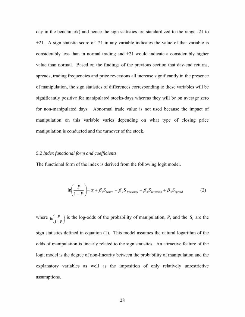
5.2 Index functional form and coefficients
The functional form of the index is derived from the following logit model.
spreadreversionfrequencyreturn SSSSP
P43211
ln ββββα ++++=⎟⎠⎞
⎜⎝⎛−
(2)
where ⎟⎠⎞
⎜⎝⎛
− PP
1ln is the log-odds of the probability of manipulation, P, and the are the
sign statistics defined in equation (1). This model assumes the natural logarithm of the
odds of manipulation is linearly related to the sign statistics. An attractive feature of the
logit model is the degree of non-linearity between the probability of manipulation and the
explanatory variables as well as the imposition of only relatively unrestrictive
assumptions.
iS
28

We estimate the coefficients of this model by performing binary logistic regression using
manipulated and non-manipulated stock-days. The non-manipulated stock-days
(n=231,896) are obtained by taking, for each manipulated stock-day (n=160), all other
stocks on the corresponding market on that day. Consequently, the non-manipulated
stock-days are an accurate match of the manipulated stock-days by market and time. The
42 day benchmark periods for the non-manipulated sample are obtained in the same way
as for the manipulated sample.
Table 4 reports the results of the regression. All coefficient estimates are statistically
significant at the one percent confidence level and the signs are consistent with
expectations. That is, abnormally positive day-end return, trade frequency, spread or
price reversion increases the probability of manipulation.
< INSERT TABLE 4 HERE >
The manipulation index is derived from the regression model by setting the index equal
to the probability of manipulation. Rearranging the regression equation and inserting the
coefficient estimates we obtain the following index.
)5.10.93.40.47.7(11
spreadfrequencyreversionreturn SSSSmanip eI ++++−−+
= (3)
29
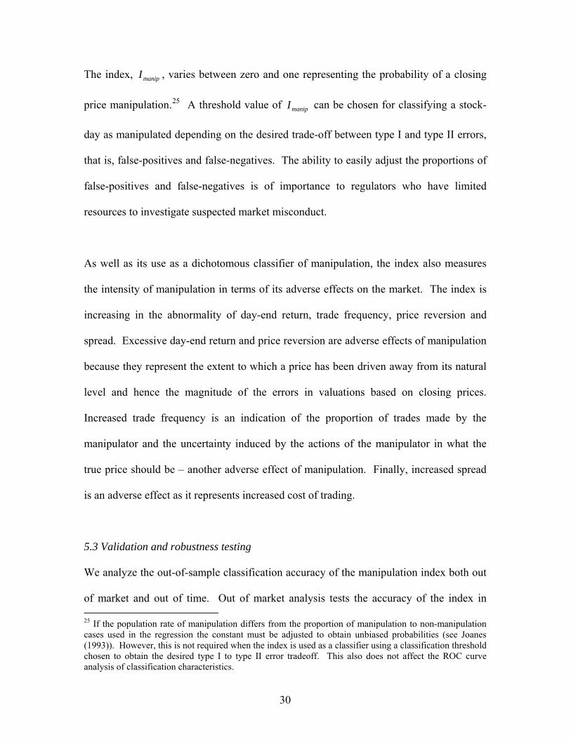
The index, , varies between zero and one representing the probability of a closing
price manipulation.
manipI
25 A threshold value of can be chosen for classifying a stock-
day as manipulated depending on the desired trade-off between type I and type II errors,
that is, false-positives and false-negatives. The ability to easily adjust the proportions of
false-positives and false-negatives is of importance to regulators who have limited
resources to investigate suspected market misconduct.
manipI
As well as its use as a dichotomous classifier of manipulation, the index also measures
the intensity of manipulation in terms of its adverse effects on the market. The index is
increasing in the abnormality of day-end return, trade frequency, price reversion and
spread. Excessive day-end return and price reversion are adverse effects of manipulation
because they represent the extent to which a price has been driven away from its natural
level and hence the magnitude of the errors in valuations based on closing prices.
Increased trade frequency is an indication of the proportion of trades made by the
manipulator and the uncertainty induced by the actions of the manipulator in what the
true price should be – another adverse effect of manipulation. Finally, increased spread
is an adverse effect as it represents increased cost of trading.
5.3 Validation and robustness testing
We analyze the out-of-sample classification accuracy of the manipulation index both out
of market and out of time. Out of market analysis tests the accuracy of the index in 25 If the population rate of manipulation differs from the proportion of manipulation to non-manipulation cases used in the regression the constant must be adjusted to obtain unbiased probabilities (see Joanes (1993)). However, this is not required when the index is used as a classifier using a classification threshold chosen to obtain the desired type I to type II error tradeoff. This also does not affect the ROC curve analysis of classification characteristics.
30
predicting manipulation on markets not used in its estimation. Similarly, out of time
analysis tests the index in a period of time not used in fitting it. These analyses
demonstrate the practical applicability of the index. As discussed previously, data on
actual manipulation cases is very difficult to obtain and in many markets it is not made
publicly available. Hence, for the majority of world markets it is not possible to
individually estimate the index for each market. Good out of market performance also
allows this index to be applied in cross-market studies without bias. One practical use of
the index is to estimate it on historic data and then apply it to predicting manipulation
forward in time. The ability to do this is verified by out-of-time analysis.
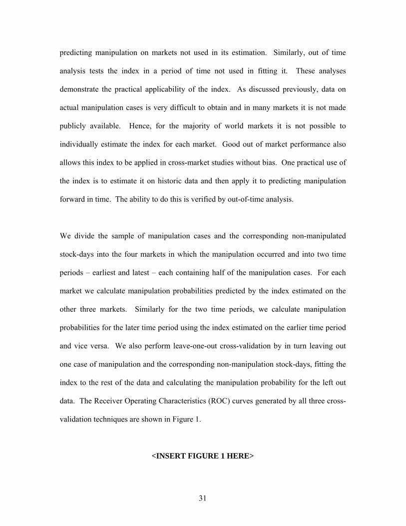
We divide the sample of manipulation cases and the corresponding non-manipulated
stock-days into the four markets in which the manipulation occurred and into two time
periods – earliest and latest – each containing half of the manipulation cases. For each
market we calculate manipulation probabilities predicted by the index estimated on the
other three markets. Similarly for the two time periods, we calculate manipulation
probabilities for the later time period using the index estimated on the earlier time period
and vice versa. We also perform leave-one-out cross-validation by in turn leaving out
one case of manipulation and the corresponding non-manipulation stock-days, fitting the
index to the rest of the data and calculating the manipulation probability for the left out
data. The Receiver Operating Characteristics (ROC) curves generated by all three cross-
validation techniques are shown in Figure 1.
<INSERT FIGURE 1 HERE>
31
The ROC curve is a performance measure independent of prior probabilities and
classification thresholds.26 It is a graphical representation of the trade-off between the
proportion of true-positives, i.e. the sensitivity, and the proportion of false-positives, i.e.
one minus the specificity. In the context of detecting manipulation, it describes the
proportion of non-manipulated stock-days that will trigger manipulation alerts in order
for the test to detect a certain proportion of actual manipulation. A test with the
characteristics of any point on the ROC curve can be obtained by choosing the
corresponding classification threshold. The area under the ROC curve (AUROC) is a
robust measure by which to compare the performance of different classifiers when used
on the same sample or, as in this case, the performance of one classifier across different
samples. The AUROC represents the probability of correct prediction and is equivalent
to the Mann-Whitney-Wilcoxon two-independent sample non-parametric test statistic
(Hanley and McNeil, 1982).
The ROC curves under all three cross-validation regimes are significantly above the
ascending diagonal line that represents a classifier only as good as chance. Consistent
with this, the lower bounds of the 95% confidence intervals for the AUROC shown in
Table 5 are well above 0.5 indicating the index performs considerably better than chance
in predicting manipulation out of market and out of time. Table 5 also shows that the
95% confidence intervals for the AUROC of the three cross-validation techniques
overlap and that the point estimates differ by less than two percent. This is strong
26 For a more detailed description of ROC curves applied in a financial modeling context see Tang and Chi (2005) and Stein (2005).
32

evidence that the index is robust to different markets and time periods and can, with a
relatively high level of accuracy, predict manipulation in markets and time periods not
used in its estimation.
<INSERT TABLE 5 HERE>
To provide an example of the accuracy of the index at a point on the leave-one-out cross-
validation ROC curve that may be used in a regulatory application, a threshold value of
Imanip=0.78 results in approximately 77% of manipulated stock-days classified correctly
with 23% of non-manipulated stock-days being misclassified as manipulated. More
realistically a market regulator with limited resources would first investigate cases with
the highest probability of manipulation scores and continue to investigate lower
probability cases as far as their resources allow. Higher index scores have a lower
probability of misclassification.
Two systematic components of the false-positive rate are late-day news and undetected
manipulation. With regard to the latter, it is likely that the non-manipulated sample we
use does contain some manipulated stock-days that have not been prosecuted. This
causes the classification accuracy to be understated as the index should classify these as
manipulated closing prices although in the data they are labeled not manipulated.
Late-day news is likely to create abnormal day-end trading activity that may resemble
manipulation and therefore lead to false-positive classification. In a regulatory
33
application this is relatively easily managed by checking for late-day news when
examining manipulation alerts. In an academic application of the index, this component
of the error can be minimized by coupling the index with a news database and
disregarding manipulation classifications that coincide with late-day news.
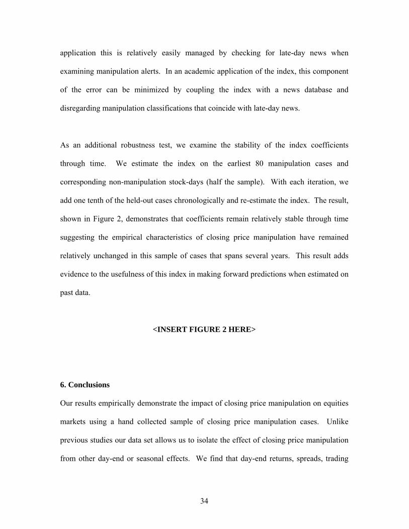
As an additional robustness test, we examine the stability of the index coefficients
through time. We estimate the index on the earliest 80 manipulation cases and
corresponding non-manipulation stock-days (half the sample). With each iteration, we
add one tenth of the held-out cases chronologically and re-estimate the index. The result,
shown in Figure 2, demonstrates that coefficients remain relatively stable through time
suggesting the empirical characteristics of closing price manipulation have remained
relatively unchanged in this sample of cases that spans several years. This result adds
evidence to the usefulness of this index in making forward predictions when estimated on
past data.
<INSERT FIGURE 2 HERE>
6. Conclusions
Our results empirically demonstrate the impact of closing price manipulation on equities
markets using a hand collected sample of closing price manipulation cases. Unlike
previous studies our data set allows us to isolate the effect of closing price manipulation
from other day-end or seasonal effects. We find that day-end returns, spreads, trading
34
activity and price reversions all increase significantly in the presence of manipulation.
We find interesting differences in the magnitudes of these impacts for different types of
manipulation and different turnover of stocks, particularly in the effect of manipulation
on trade size. Based on these findings we construct an index to measure the probability
and intensity of closing price manipulation using logistic regression of non-parametric
measures. We demonstrate the robustness of this index to application out of time and out
of market and obtain estimates of its classification accuracy.
The closing price manipulation index derived in this paper creates opportunities for a
range of future research in market integrity. Theoretical models27 of market
manipulation can be validated more accurately than they have been to date as can
empirical research that uses less rigorous indices or proxies for manipulation. This index
can be applied through time and across markets to examine the relationship between
manipulation and market design features, regulatory environment, and surveillance
effort. A more thorough understanding of these relationships has implications for
strategies to reduce the incidence of manipulation. The prevalence of the various
motivations for manipulation can be quantified using this index by analyzing the kinds of
days that exhibit an increased rate of manipulation. The characteristics of firms more
frequently manipulated can be identified. These two insights would allow more efficient
use of scare regulatory and surveillance resources.
27 For example Kumar and Seppi (1992), Bernhardt et al. (2005), Hillion and Suominen (2004) and Felixson and Pelli (1999).
35
References
Aggarwal, Rajesh K., and Guojun Wu, 2006, Stock market manipulations, Journal of Business 79, 1915-1953. Allen, Franklin and Douglas Gale, 1992, Stock-price manipulation, The Review of Financial Studies 5, 503-529. Allen, Franklin, Lubomir Litov, and Jianping Mei, 2006, Large investors, price manipulation, and limits to arbitrage: Anatomy of market corners, SSRN Working paper 01/14/2006. Ariel, Robert A., 1987, A monthly effect in stock returns, Journal of Financial Economics 18, 161-174. Bernhardt, Dan, and Ryan J. Davies, 2005, Painting the tape: Aggregate evidence. Economics Letters 89, 306-311. Bernhardt, Dan, Ryan J. Davies, and Harvey Westbrook Jr., 2005, Smart fund managers? Stupid money?, University of Illinois Working paper 03/21/2005. Carhart, Mark, Ron Kaniel, David Musto, and Adam Reed, 2002, Leaning for the tape: Evidence of gaming behavior in equity mutual funds, Journal of Finance 57, 661–693. Chamberlain, Trevor W., C. Sherman Cheung, and Clarence C.Y. Kwan, 1989, Expiration-day effects of index futures and options: Some Canadian evidence, Financial Analysts Journal 45, 67–71. Corredor, Pilar, Pedro Lechon, and Rafael Santamaria, 2001, Option-expiration effects in small markets: The Spanish Stock Exchange. Journal of Futures Markets 21, 905–928. Feinstein, Jonathan S., 1990, Detection controlled estimation, Journal of Law and Economics 33, 233-276. Feinstein, Jonathan S., 1991, An econometric analysis of income tax evasion and its detection, Rand Journal of Economics 22, 14-35. Felixson, Karl, and Anders Pelli, 1999, Day end returns – stock price manipulation, Journal of Multinational Financial Management 9, 95-127. Hanley, James A., and Barbara J. McNeil, 1982, The meaning and use of the area under a receiver operating characteristics curve, Radiology 143, 29–36. Harris, Lawrence, 1989, A day-end transaction price anomaly, Journal of Financial and Quantitative Analysis 24, 29-45.
36
Hillion, Pierre, and Matti Suominen, 2004, The manipulation of closing prices, Journal of Financial Markets 7, 351–75. Joanes, Derrick N., 1993, Reject inference applied to logistic regression for credit scoring, Journal of Mathematics Applied in Business & Industry 5, 35-43. Keim, Donald, 1983, Size-related anomalies and stock return seasonality: Further empirical evidence, Journal of Financial Economics 12, 13-32. Kumar, Praveen, and Duane J. Seppi, 1992, Futures manipulation with cash settlement, Journal of Finance 47, 1485–1502. Mei, Jianping, Guojun Wu, and Chunsheng Zhou, 2004, Behavior based manipulation – Theory and prosecution evidence, Unpublished manuscript, New York University. Meulbroek, Lisa K. and Carolyn Hart, 1997, The effect of illegal insider trading on takeover premia, European Finance Review 1, 51– 80. Pagano, Michael S., and Robert A. Schwartz, 2003, A closing call’s impact on market quality at Euronext Paris, Journal of Financial Economics 68, 439-484. Poirier, Dale J., 1980, Partial observability in bivariate probit models, Journal of Econometrics 12, 209-217. Pritchard, Adam C., 2003, Self-regulation and securities markets, Regulation 26, 32–39. Ritter, Jay, 1988, The buying and selling behavior of individual investors at the turn of the year, Journal of Finance 43, 701-717. Roll, Richard W., 1983, Vast ist das? The turn of the year effect and the return premium of small firms, Journal of Portfolio management 9, 18-28. Stein, Roger M., 2005, The relationship between default prediction and lending profits: Integrating ROC analysis and loan pricing, Journal of Banking and Finance 29, 1213-1236. Stoll, Hans R., and Robert E. Whaley, 1987, Program trading and expiration-day effects. Financial Analysts Journal 43, 16–28. Stoll, Hans R., and Robert E. Whaley, 1991, Expiration-day effects: What has changed? Financial Analysts Journal 47, 58–72. Tang, Tseng-Chung, and Li-Chiu Chi, 2005, Predicting multilateral trade credit risks: Comparisons of logit and fuzzy logic models using ROC curve analysis, Expert Systems with Applications 28, 547-556.
37
Thomas, S., 1998, End of day patterns on the Paris bourse after implementation of a call auction, Global Equity Markets Conference Proceedings, Bourse de Paris-NYSE. Wood, Robert A., Thomas H. McInish, J. Keith Ord, 1985, An investigation of transactions data for NYSE stocks, The Journal of Finance 40, 723-739. Xiaoyan Ni, Sophie, Neil D. Pearson, Allen M. Poteshman, 2005, Stock price clustering on option expiration dates, Journal of Financial Economics 78, 49-87.
38
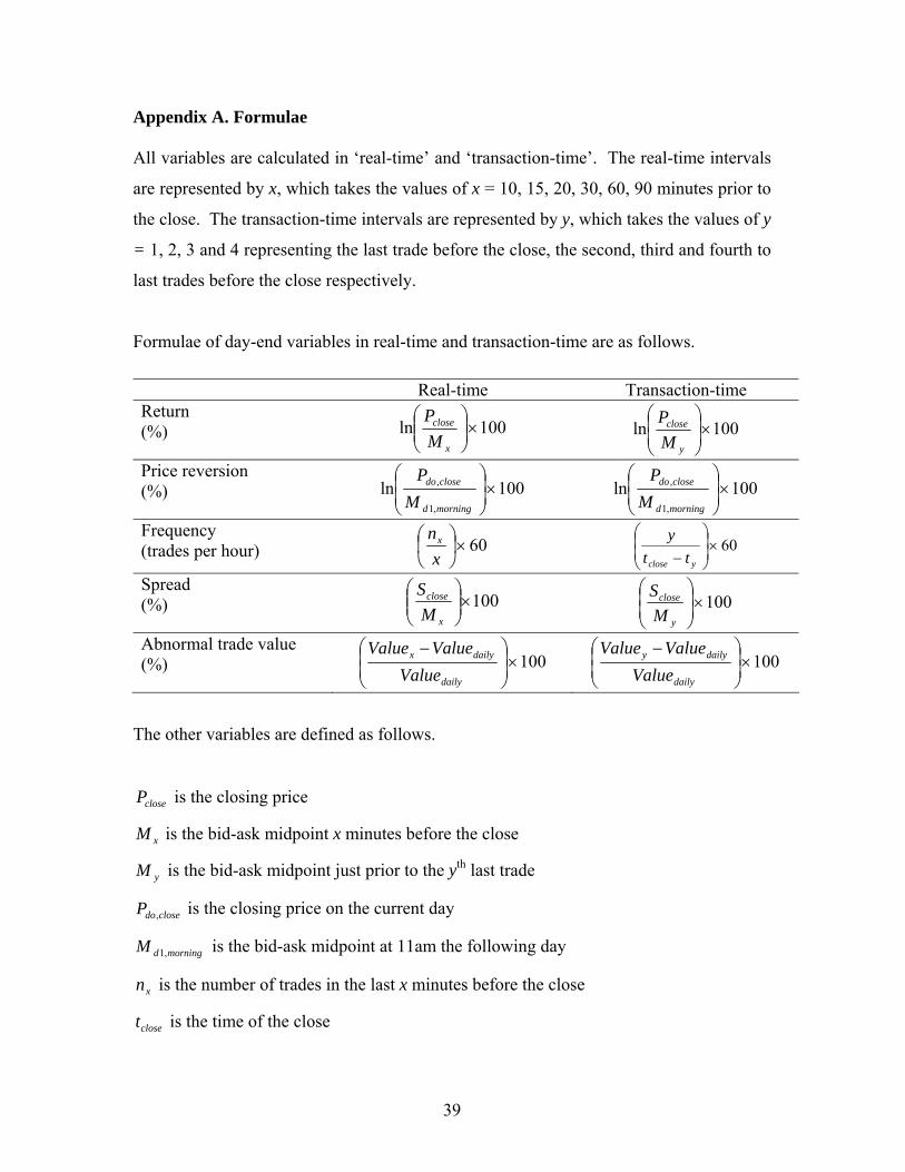
Appendix A. Formulae All variables are calculated in ‘real-time’ and ‘transaction-time’. The real-time intervals
are represented by x, which takes the values of x = 10, 15, 20, 30, 60, 90 minutes prior to
the close. The transaction-time intervals are represented by y, which takes the values of y
= 1, 2, 3 and 4 representing the last trade before the close, the second, third and fourth to
last trades before the close respectively.
Formulae of day-end variables in real-time and transaction-time are as follows. Real-time Transaction-time Return (%) 100ln ×⎟⎟
⎠
⎞⎜⎜⎝
⎛
x
close
MP
100ln ×⎟⎟⎠
⎞⎜⎜⎝
⎛
y
close
MP
Price reversion (%) 100ln
,1
, ×⎟⎟⎠
⎞⎜⎜⎝
⎛
morningd
closedo
MP
100ln,1
, ×⎟⎟⎠
⎞⎜⎜⎝
⎛
morningd
closedo
MP
Frequency (trades per hour) 60×⎟
⎠⎞
⎜⎝⎛
xnx 60×⎟
⎟⎠
⎞⎜⎜⎝
⎛
− yclose tty
Spread (%) 100×⎟⎟
⎠
⎞⎜⎜⎝
⎛
x
close
MS 100×⎟
⎟⎠
⎞⎜⎜⎝
⎛
y
close
MS
Abnormal trade value (%) 100×⎟
⎟⎠
⎞⎜⎜⎝
⎛ −
daily
dailyx
ValueValueValue
100×⎟⎟⎠
⎞⎜⎜⎝
⎛ −
daily
dailyy
ValueValueValue
The other variables are defined as follows.
closeP is the closing price
xM is the bid-ask midpoint x minutes before the close
yM is the bid-ask midpoint just prior to the yth last trade
closedoP , is the closing price on the current day
morningdM ,1 is the bid-ask midpoint at 11am the following day
xn is the number of trades in the last x minutes before the close
closet is the time of the close
39
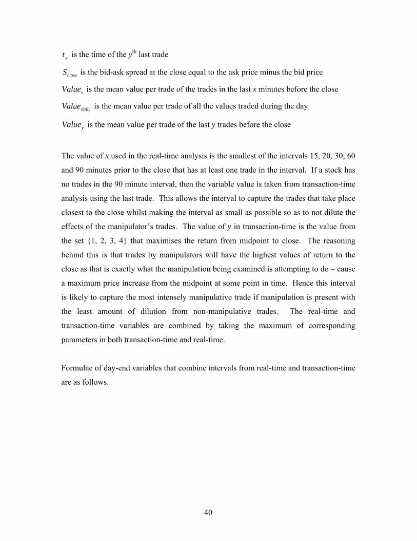
yt is the time of the yth last trade
closeS is the bid-ask spread at the close equal to the ask price minus the bid price
xValue is the mean value per trade of the trades in the last x minutes before the close
dailyValue is the mean value per trade of all the values traded during the day
yValue is the mean value per trade of the last y trades before the close
The value of x used in the real-time analysis is the smallest of the intervals 15, 20, 30, 60
and 90 minutes prior to the close that has at least one trade in the interval. If a stock has
no trades in the 90 minute interval, then the variable value is taken from transaction-time
analysis using the last trade. This allows the interval to capture the trades that take place
closest to the close whilst making the interval as small as possible so as to not dilute the
effects of the manipulator’s trades. The value of y in transaction-time is the value from
the set {1, 2, 3, 4} that maximises the return from midpoint to close. The reasoning
behind this is that trades by manipulators will have the highest values of return to the
close as that is exactly what the manipulation being examined is attempting to do – cause
a maximum price increase from the midpoint at some point in time. Hence this interval
is likely to capture the most intensely manipulative trade if manipulation is present with
the least amount of dilution from non-manipulative trades. The real-time and
transaction-time variables are combined by taking the maximum of corresponding
parameters in both transaction-time and real-time.
Formulae of day-end variables that combine intervals from real-time and transaction-time
are as follows.
40
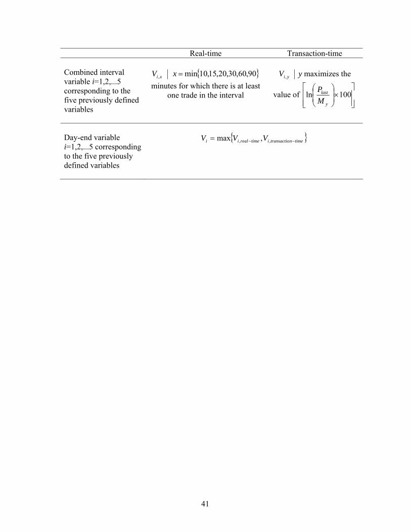
Real-time Transaction-time Combined interval variable i=1,2,...5 corresponding to the five previously defined variables
xiV , { }90,60,30,20,15,10min=x
minutes for which there is at least one trade in the interval
yiV , y maximizes the
value of ⎥⎥⎦
⎤
⎢⎢⎣
⎡×⎟⎟⎠
⎞⎜⎜⎝
⎛100ln
y
last
MP
Day-end variable i=1,2,...5 corresponding to the five previously defined variables
{ }timentransactioitimerealii VVV −−= ,, ,max
41
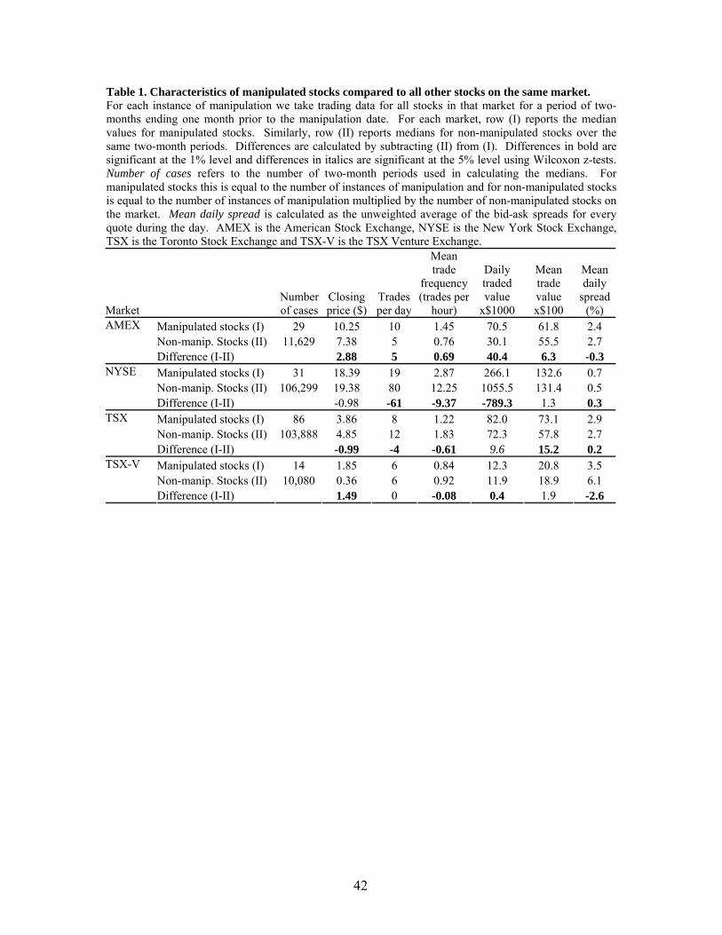
Table 1. Characteristics of manipulated stocks compared to all other stocks on the same market. For each instance of manipulation we take trading data for all stocks in that market for a period of two-months ending one month prior to the manipulation date. For each market, row (I) reports the median values for manipulated stocks. Similarly, row (II) reports medians for non-manipulated stocks over the same two-month periods. Differences are calculated by subtracting (II) from (I). Differences in bold are significant at the 1% level and differences in italics are significant at the 5% level using Wilcoxon z-tests. Number of cases refers to the number of two-month periods used in calculating the medians. For manipulated stocks this is equal to the number of instances of manipulation and for non-manipulated stocks is equal to the number of instances of manipulation multiplied by the number of non-manipulated stocks on the market. Mean daily spread is calculated as the unweighted average of the bid-ask spreads for every quote during the day. AMEX is the American Stock Exchange, NYSE is the New York Stock Exchange, TSX is the Toronto Stock Exchange and TSX-V is the TSX Venture Exchange.
Market Number of cases
Closing price ($)
Trades per day
Mean trade
frequency (trades per
hour)
Daily traded value
x$1000
Mean trade value x$100
Mean daily
spread (%)
Manipulated stocks (I) 29 10.25 10 1.45 70.5 61.8 2.4 Non-manip. Stocks (II) 11,629 7.38 5 0.76 30.1 55.5 2.7
AMEX
Difference (I-II) 2.88 5 0.69 40.4 6.3 -0.3 Manipulated stocks (I) 31 18.39 19 2.87 266.1 132.6 0.7 Non-manip. Stocks (II) 106,299 19.38 80 12.25 1055.5 131.4 0.5
NYSE
Difference (I-II) -0.98 -61 -9.37 -789.3 1.3 0.3 Manipulated stocks (I) 86 3.86 8 1.22 82.0 73.1 2.9 Non-manip. Stocks (II) 103,888 4.85 12 1.83 72.3 57.8 2.7
TSX
Difference (I-II) -0.99 -4 -0.61 9.6 15.2 0.2 Manipulated stocks (I) 14 1.85 6 0.84 12.3 20.8 3.5 Non-manip. Stocks (II) 10,080 0.36 6 0.92 11.9 18.9 6.1
TSX-V
Difference (I-II) 1.49 0 -0.08 0.4 1.9 -2.6
42
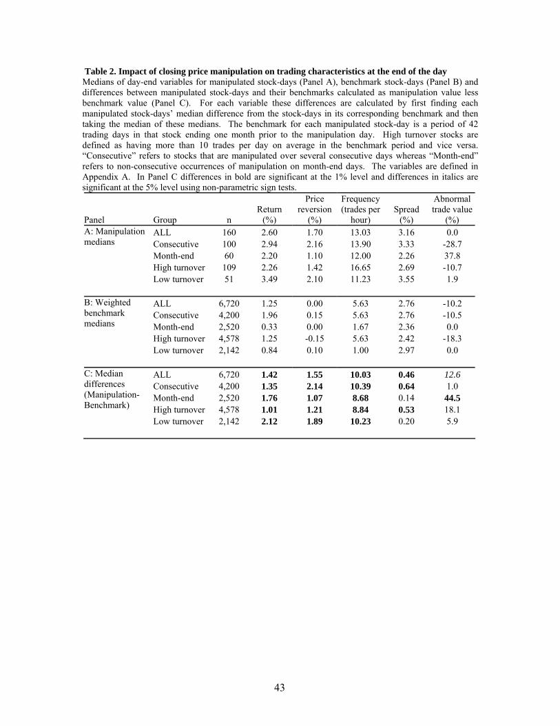
Table 2. Impact of closing price manipulation on trading characteristics at the end of the day Medians of day-end variables for manipulated stock-days (Panel A), benchmark stock-days (Panel B) and differences between manipulated stock-days and their benchmarks calculated as manipulation value less benchmark value (Panel C). For each variable these differences are calculated by first finding each manipulated stock-days’ median difference from the stock-days in its corresponding benchmark and then taking the median of these medians. The benchmark for each manipulated stock-day is a period of 42 trading days in that stock ending one month prior to the manipulation day. High turnover stocks are defined as having more than 10 trades per day on average in the benchmark period and vice versa. “Consecutive” refers to stocks that are manipulated over several consecutive days whereas “Month-end” refers to non-consecutive occurrences of manipulation on month-end days. The variables are defined in Appendix A. In Panel C differences in bold are significant at the 1% level and differences in italics are significant at the 5% level using non-parametric sign tests.
Panel Group n Return
(%)
Price reversion
(%)
Frequency (trades per
hour) Spread
(%)
Abnormal trade value
(%) ALL 160 2.60 1.70 13.03 3.16 0.0 Consecutive 100 2.94 2.16 13.90 3.33 -28.7 Month-end 60 2.20 1.10 12.00 2.26 37.8 High turnover 109 2.26 1.42 16.65 2.69 -10.7
A: Manipulation medians
Low turnover 51 3.49 2.10 11.23 3.55 1.9
ALL 6,720 1.25 0.00 5.63 2.76 -10.2 Consecutive 4,200 1.96 0.15 5.63 2.76 -10.5 Month-end 2,520 0.33 0.00 1.67 2.36 0.0 High turnover 4,578 1.25 -0.15 5.63 2.42 -18.3
B: Weighted benchmark medians
Low turnover 2,142 0.84 0.10 1.00 2.97 0.0
ALL 6,720 1.42 1.55 10.03 0.46 12.6 Consecutive 4,200 1.35 2.14 10.39 0.64 1.0 Month-end 2,520 1.76 1.07 8.68 0.14 44.5 High turnover 4,578 1.01 1.21 8.84 0.53 18.1
C: Median differences (Manipulation-Benchmark)
Low turnover 2,142 2.12 1.89 10.23 0.20 5.9
43

Table 3. Robustness tests of day-end variable definition and potential sample selection bias The excess variables are differences between manipulated stock-days and their benchmarks (manipulation value less benchmark value) as per Table 2 Panel C. For each day-end variable (defined in Appendix A) these differences are calculated by first finding each manipulated stock-days’ median difference from the stock-days in its corresponding benchmark and then taking the median of these medians. The benchmark for each manipulated stock-day is a period of 42 trading days in that stock ending one month prior to the manipulation day. Combined interval refers to variable values calculated by combining values from several day-end intervals as defined in Appendix A and used in Table2 Panel C. Last 30 minutes refers to variable values calculated over the last 30 minutes before the close and in the absence of trades in this interval then from the last trade to the close. Last 4 trades refers to variable values calculated over the last four trades before the close and on days with less than four trades, then from the first trade to the close. All manipulation includes every instance of manipulation identified from the litigation releases and Undetected proxy excludes from the full manipulation sample five instances from each case of manipulation with the greatest absolute day-end return. n is the number of instances of closing price manipulation. Differences in bold are significant at the 1% level and differences in italics are significant at the 5% level using non-parametric sign tests.
Sample n
Excess return (%)
Excess price
reversion (%)
Excess frequency (trades per
hour)
Excess spread
(%)
Excess abnormal
trade value (%)
All manipulation 160 1.42 1.55 10.03 0.46 12.6 Panel A: Tests of sample selection bias Undetected proxy 130 0.85 1.23 10.31 0.26 5.9 Variable type
Combined interval 160 1.42 1.55 10.03 0.46 12.6 Last 30 minutes 160 1.61 1.55 4.00 0.50 11.4
Panel B: Alternate definitions of day-end variables Last four trades 160 1.40 1.55 6.72 0.46 0.9
44
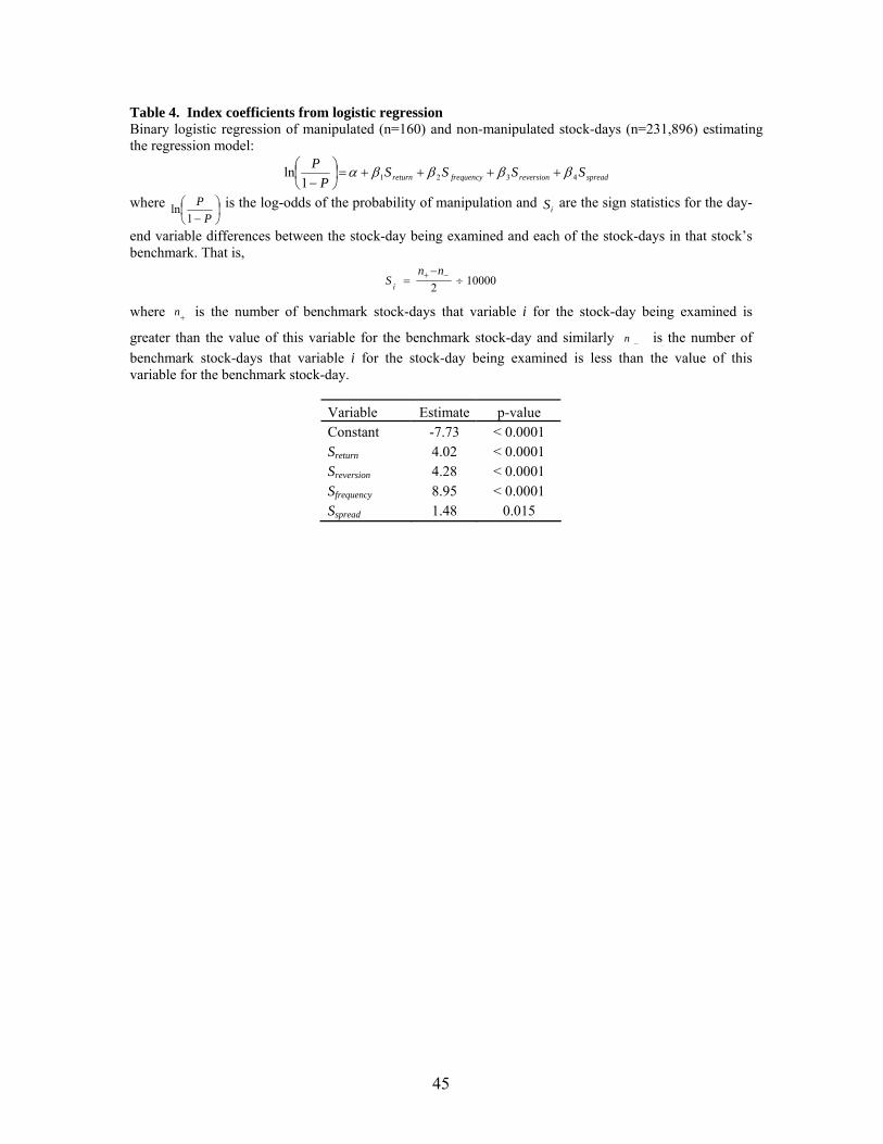
Table 4. Index coefficients from logistic regression Binary logistic regression of manipulated (n=160) and non-manipulated stock-days (n=231,896) estimating the regression model:
spreadreversionfrequencyreturn SSSSP
P43211
ln ββββα ++++=⎟⎠⎞
⎜⎝⎛−
where ⎟⎠⎞
⎜⎝⎛
− PP
1ln is the log-odds of the probability of manipulation and are the sign statistics for the day-
end variable differences between the stock-day being examined and each of the stock-days in that stock’s benchmark. That is,
iS
100002 ÷−
= −+ nnS i
where is the number of benchmark stock-days that variable i for the stock-day being examined is
greater than the value of this variable for the benchmark stock-day and similarly is the number of benchmark stock-days that variable i for the stock-day being examined is less than the value of this variable for the benchmark stock-day.
+n
−n
Variable Estimate p-value Constant -7.73 < 0.0001 Sreturn 4.02 < 0.0001 Sreversion 4.28 < 0.0001 Sfrequency 8.95 < 0.0001 Sspread 1.48 0.015
45
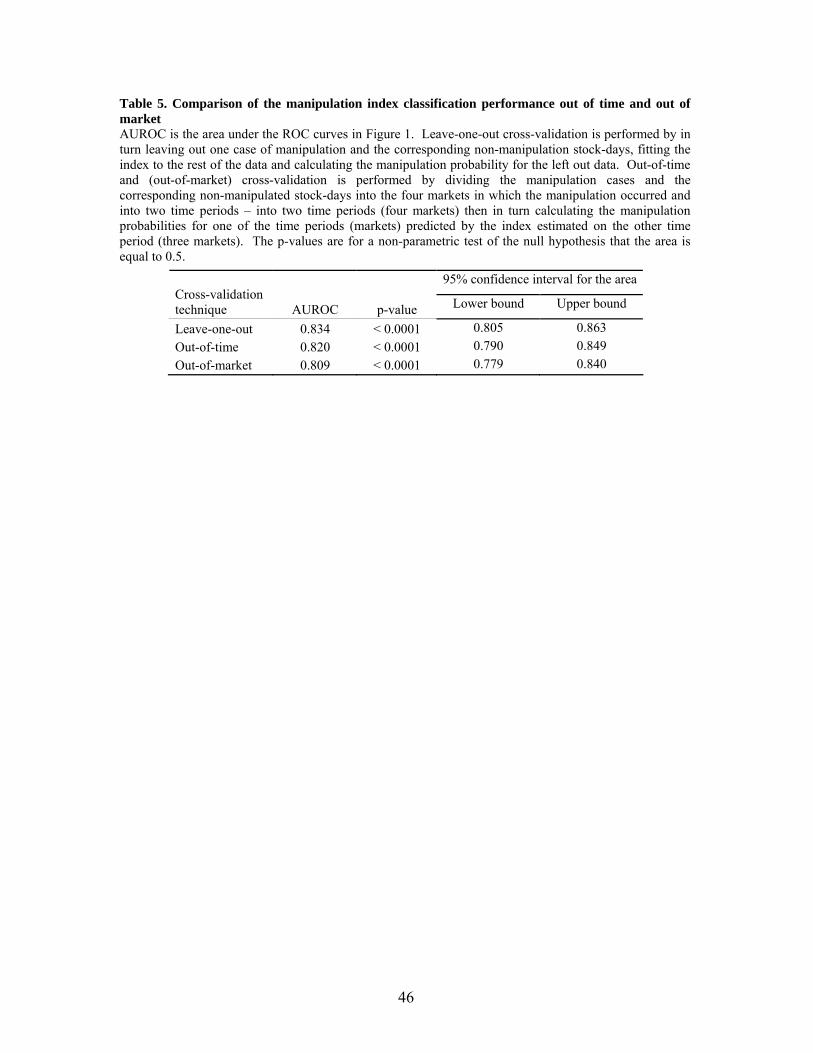
Table 5. Comparison of the manipulation index classification performance out of time and out of market AUROC is the area under the ROC curves in Figure 1. Leave-one-out cross-validation is performed by in turn leaving out one case of manipulation and the corresponding non-manipulation stock-days, fitting the index to the rest of the data and calculating the manipulation probability for the left out data. Out-of-time and (out-of-market) cross-validation is performed by dividing the manipulation cases and the corresponding non-manipulated stock-days into the four markets in which the manipulation occurred and into two time periods – into two time periods (four markets) then in turn calculating the manipulation probabilities for one of the time periods (markets) predicted by the index estimated on the other time period (three markets). The p-values are for a non-parametric test of the null hypothesis that the area is equal to 0.5.
95% confidence interval for the area Cross-validation technique AUROC p-value Lower bound Upper bound
Leave-one-out 0.834 < 0.0001 0.805 0.863 Out-of-time 0.820 < 0.0001 0.790 0.849 Out-of-market 0.809 < 0.0001 0.779 0.840
46
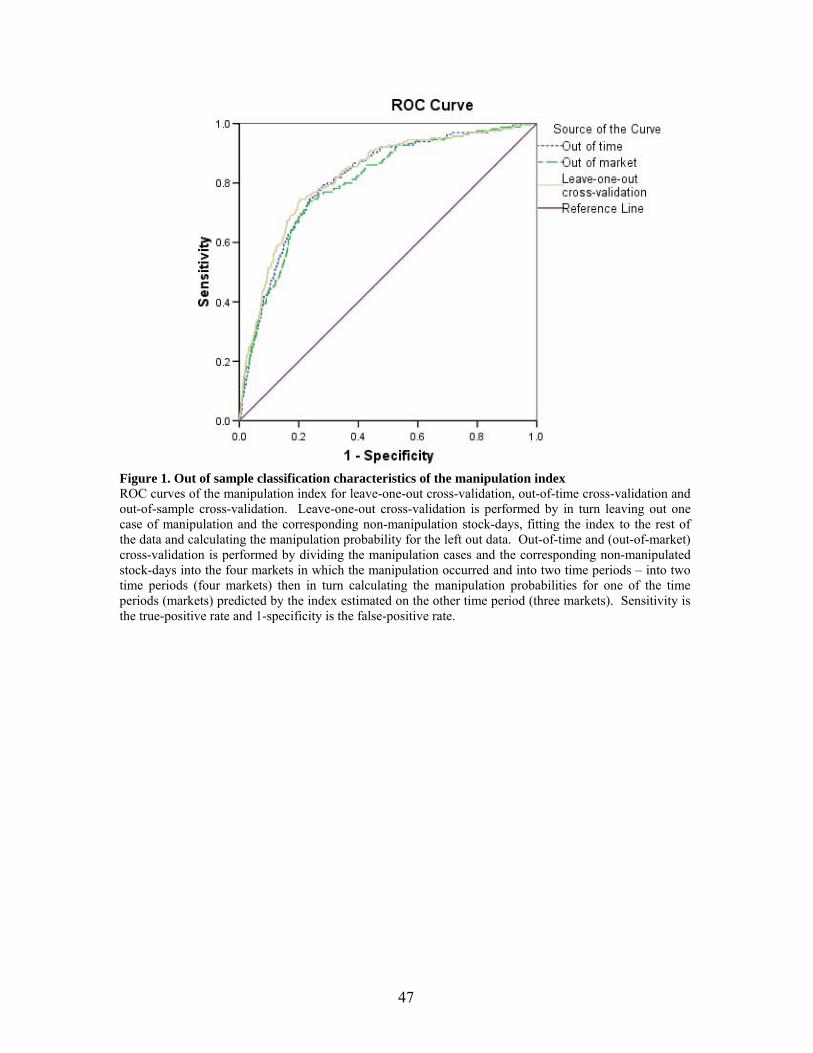
Figure 1. Out of sample classification characteristics of the manipulation index ROC curves of the manipulation index for leave-one-out cross-validation, out-of-time cross-validation and out-of-sample cross-validation. Leave-one-out cross-validation is performed by in turn leaving out one case of manipulation and the corresponding non-manipulation stock-days, fitting the index to the rest of the data and calculating the manipulation probability for the left out data. Out-of-time and (out-of-market) cross-validation is performed by dividing the manipulation cases and the corresponding non-manipulated stock-days into the four markets in which the manipulation occurred and into two time periods – into two time periods (four markets) then in turn calculating the manipulation probabilities for one of the time periods (markets) predicted by the index estimated on the other time period (three markets). Sensitivity is the true-positive rate and 1-specificity is the false-positive rate.
47
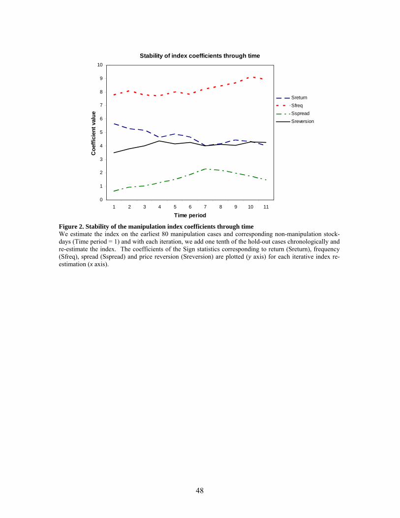
Stability of index coefficients through time
0
1
2
3
4
5
6
7
8
9
10
1 2 3 4 5 6 7 8 9 10 11
Time period
Coe
ffici
ent v
alue
SreturnSfreqSspreadSreversion
Figure 2. Stability of the manipulation index coefficients through time We estimate the index on the earliest 80 manipulation cases and corresponding non-manipulation stock-days (Time period = 1) and with each iteration, we add one tenth of the hold-out cases chronologically and re-estimate the index. The coefficients of the Sign statistics corresponding to return (Sreturn), frequency (Sfreq), spread (Sspread) and price reversion (Sreversion) are plotted (y axis) for each iterative index re-estimation (x axis).
48