measurement theory item response theory what is...
TRANSCRIPT

1
1
Item Response Theory
Ryan P. BowlesMay 17, 2005
2
Outline• IRT as model-based measurement
– Measurement theory– Why sum scores are insufficient
• Rasch measurement• IRT models• Advanced topics in IRT
– Linking– DIF– CAT
• IRT as explanatory models– Item predictor models– Multidimensional models– Dynamic models
3
Item Response Theory as Model-Based Measurement
4
What is measurement?• Main use of IRT is in psychological
measurement– psychological measurement = measurement in the
social sciences = measurement of latent traits• What is measurement?• What makes measurement meaningful?• How is meaningful measurement achieved?
Hand, D. J. (1996). Statistics and the theory of measurement. Journal of the Statistical Society of America, 159, 445-492.
Michell, J. (1990). An introduction to the logic of psychological measurement. Hillsdale, NJ: Erlbaum.
5
Representational view• Standard conceptualization of
psychological measurement• “Assignment of numbers to objects
according to a rule” (Stevens, 1951)
6
Representational view
• Attribute(s) of interest- latent trait– E.g., print concepts knowledge, anxiety, skill
• Population of objects of measurement having the attribute(s)- subjects– E.g., kids, test-takers, teams

2
7
Representational view
• Agent of measurement- instrument– test, questionnaire
• Create a homomorphism (mapping) from the objects to the real numbers such that– each object is represented by a number– relations between the objects on the attributes
are represented by relations between the real numbers (equality, order)
8
6 ft.
Representational view
6 ft.
Heights are the same
6 ft.
Assigned numbers are the same
9
Representational view
Differences in height are the same
6’ (72”)5’5” (67”)4’10” (58”)
Differences in assigned numbers are the same
10
Representational view
• Meaningful measurement occurs when the assignment of numbers successfully achieves representation of the desired relations between objects
11
What is the appropriate way to conduct meaningful
measurement?
12
Measurement Models• A measurement model is the way numbers are
“assigned” to objects– a model is a mathematical expression of how
observed and unobserved relate to each other– use model to get an estimate of latent trait level using
observed responses– how we “choose” the numbers
• Measurement is meaningful when the model provides an appropriate number assignment– trait level estimates that reflect relations between trait
levels• What is an appropriate measurement model?

3
13
Item Response Theory
• Collection of models and associated statistical techniques for converting (usually) ordinal categorical data to trait level estimates– dichotomous: right/wrong, yes/no, win/loss– polytomous: Likert scales, other rating scales
14
IRT• Used in many contexts
– standardized educational tests: SAT, GRE, ACT, NAEP– normed psychological tests: Woodcock-Johnson– licensure and certification: nurses, systems administrators– educational standards: Lexiles– rehabilitation medicine– sports
• Two branches– IRT perspective (mechanistic)– Rasch perspective (prescriptive)
15
Mechanistic (IRT)
• Model should describe response mechanism– model process by which latent trait yields
observations– how do subjects interact with items to yield
responses?– if model is correct, then can work backwards from
responses to get trait level estimates• Measurement is successful when
– the model fully describes or closely approximates the response process
– when model fits the data16
Mechanistic (IRT)
• If not successful, then– conclude that our theory about response
process was wrong– reformulate theory– reformulate model– usually by relaxing constraints (i.e. adding
parameters)
17
Prescriptive (Rasch)
• Model should reflect properties required for measurement– define measurement properties– derive or identify model that reflects these
properties– such that measurement properties are
testable in the framework of the model• Measurement is meaningful when
– the required measurement properties are met– when data fit the model
18
Prescriptive (Rasch)
• If not successful, then– meaningful measurement cannot be achieved
with the current subjects and instrument• some items may not behave as required• latent trait may not have same meaning for all
subjects– identify and eliminate measurement
anomalies– usually by removing or replacing parts of
measurement instrument

4
19
Comparison
Rasch IRT
Model is valid If has important measurement
properties
If describes response process
Validity evidence
Data fit model Model fits data
Response to misfit
Remove anomalies
Revise theory/ model
20
Comparison
• Ongoing debate– Jaeger (1987), Fisher (1994), Andrich
(2002)• Great deal of confusion about
differences– perhaps Kuhnian incompatibility between
the paradigms (Andrich, 2002)– incorrect interpretations of results– difficulties in peer review– incompatible recommendations for practice
21
Comparison
• In practice, many similarities– both use statistical fit as evidence of
successful measurement– Rasch model is functionally equivalent to the
1PL IRT (often called Rasch) model (Andrich, 1989)
– often yield very similar results • correlations between ability estimates with Rasch
or IRT are above .9 if the data-model fit is reasonable
22
Comparison
• Can straddle the fence– Accept measurement properties as ideal
but relax when model becomes untenable for a given data set
– Proponents of IRT perspective sometimes eliminate observations because of undesired properties (e.g., multidimensionality)
– Proponents of Rasch perspective sometimes generalize model at expense of relaxation of measurement properties (e.g., mixed Rasch model)
23
Sum scores
• So where does typical practice of summing responses fall in this?
• Two ways to looks at sum scores– operationalism– classical test theory
24
Operationalism
• Alternative to representational measurement• Attribute is defined by the instrument
– no more and no less• No assumption of an unobservable reality
– no latent attributes– as soon as you give a psychological name to the
attribute, you are in a gray area between operationalism and representationalism
• Example: SAT

5
25
Operationalism
• Meaningful measurement is achieved if it is useful
• Usefulness stems from convenience, widespread use, and/or predictive power– no theoretical considerations or evidence of
meaningful measurement is needed– goal of SAT is to predict college success
26
Operationalism
• Measurement in the social sciences is generally representational– social scientists routinely hypothesize
latent attributes that can only be approximated by measurement procedure
27
Classical Test Theory
• Representational way to look at sum scores: Classical Test Theory (CTT)– aka True Score Theory
X = T + E
28
CTT
• Simplistic view of the response process• Mostly untestable• Items are essentially irrelevant
– item effects are ignored– item properties are not linked to behavior– no clear way to compare item functioning
across non-equivalent samples
29
CTT
• Items must be regarded as fixed– difficult to generalize to new items– dealing with different tests is awkward
• test parallelism or test equating– dealing with missing data is very awkward
• Measurement error is same for all subjects– but we cannot measure everyone equally well
30
General Principles of IRT
6
31
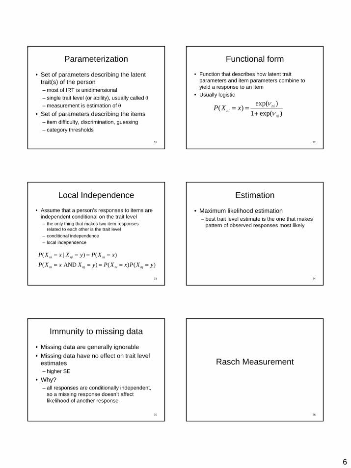
Parameterization
• Set of parameters describing the latent trait(s) of the person– most of IRT is unidimensional– single trait level (or ability), usually called θ – measurement is estimation of θ
• Set of parameters describing the items– item difficulty, discrimination, guessing– category thresholds
32
Functional form
• Function that describes how latent trait parameters and item parameters combine to yield a response to an item
• Usually logistic
exp( )( )1 exp( )
nini
ni
P X x νν
= =+
33
Local Independence
• Assume that a person’s responses to items are independent conditional on the trait level– the only thing that makes two item responses
related to each other is the trait level– conditional independence– local independence
( | ) ( )
( AND ) ( ) ( )ni nj ni
ni nj ni nj
P X x X y P X x
P X x X y P X x P X y
= = = =
= = = = =
34
Estimation
• Maximum likelihood estimation– best trait level estimate is the one that makes
pattern of observed responses most likely
35
Immunity to missing data
• Missing data are generally ignorable• Missing data have no effect on trait level
estimates– higher SE
• Why?– all responses are conditionally independent,
so a missing response doesn’t affect likelihood of another response
36
Rasch Measurement

7
37
Measurement PropertiesSpecific Objectivity:
“the comparison of any two subjects can be carried out in such a way that no other parameters are involved than those of the two subjects, neither the parameter of any other subject nor any of the stimulus (i.e., measurement instrument) parameters” (Rasch, 1966, p. 92)
– separability, test-free measurement, sample independence
38
Measurement Properties
• Existence of sufficient statistic• Interval level measurement
– additive conjoint measurement
• Objective measurement• Fundamental measurement
39
History
Georg Rasch Ben Wright Gerhard Fischer
40
The Rasch (1960/1980) model
• Note that you can add a fixed amount to all trait levels (θ) and item difficulties (β) and get the same probability– need identification constraint– mean item difficulty = 0– mean trait level = 0
exp( )( 1)1 exp( )
n ini
n i
P X θ βθ β
−= =
+ −( 1)ln( 0)
nin i
ni
P XP X
θ β⎛ ⎞=
= −⎜ ⎟=⎝ ⎠
41
00.10.20.30.40.50.60.70.80.9
1
-4 -3 -2 -1 0 1 2 3 4
Trait Level (theta)
Prob
abili
ty
β = -1
β = 0 β = 1
42
What you need
• Using the Rasch model requires– an instrument designed to measure a single
latent trait– dichotomous data– orderable responses (i.e., you have to know
which response indicates more of the latent trait)
– multiple items (10 or more?)– multiple subjects (at least 10? at least 300?)

8
43
Letters data
• Example: Letters data– Justice, Pence, Bowles, & Wiggins (2005)– What (print) letters are easiest for kids to
learn?• 339 preschool kids• 26 letters (PALS)• Winsteps
– winsteps.com
44
Data file
100110000000000000000000000000100211011000100010100010000100100301011000001100111000000110100411101100101011101011101111100501001010011000000000000100100600000100010000000001010000100700000000000000000000001000100800000000000000000000000000100911000000000000000000001100101011101111011111111111011110…
ID Responses
45
Control file&INSTTITLE='Letters data'data=letters_forWinsteps.prnITEM1=5NI=26CODES=01&ENDAB…ZEND NAMES
Run Winsteps46
Analysis
1. Summary statistics (Table 3.2)2. Person-item map (Table 1)
– aka Wright plot3. Item fit (Table 14, or 10, 13, 15)
– unexpected responses (Table 10)4. Person fit (Table 6, or 17, 18, 19)
– unexpected responses (Table 6)
47
Fit analysis
• Two common Rasch fit statistics– infit and outfit
• Both are based on response residualXni - E(Xni) = Xni – P(Xni)Ex.: if response is 1 (correct) and expectation
(probability) is .9, then residual is .1• Different weightings
48
Fit analysis
• Infit– information-weighted fit– relatively sensitive to patterns of misfit– conservative, so misfit indicated by infit is
likely important

9
49
Fit analysis
• Outfit– outlier-sensitive fit– relatively sensitive to outliers, or highly
unexpected responses– more liberal, so misfit indicated by outfit may
be unimportant – one highly unexpected response (e.g., from
miscoding) may be enough to indicate substantial misfit
50
Fit analysis
• Two forms• Mean-square
– indicates amount of misfit– expectation is 1– values higher than 1 indicate more noise
(randomness, error) than expected– values below 1 indicate less information than
expected (redundancy)
51
Fit analysis
– Cutoffs depend on goals– Conservative (Smith & Suh, 2002): .9 to 1.1– Typical (Wright & Linacre, 1994): .7 to 1.3– Liberal (Wright & Linacre, 1994): .6 to 1.4
• Standardized– converted to approximate standard normal
distribution– significant misfit: <-2 or >2
52
Fit analysis
• What should you use?– matter of opinion– I prefer to use mean-square for items and
concentrate on standardized for persons
53
Fit analysis
• Why does an item misfit?– assesses a different dimension– multiple correct answers– contaminated by irrelevant factors
• answer given away by another item• display is hard to read
54
Fit analysis
• Why does a person misfit?– not answering based on trait of interest
• guessing• inattention• test anxiety• fatigue• learning from other items

10
55
Fit analysis
If something misfits, what should you do?1. Reformulate model to relax assumptions
– IRT method, not appropriate for Rasch analysis2. Eliminate misfitting data
– remove misfitting items or persons– remove specific data points (if you can identify
source of misfit)3. Eliminate misfitting data, rerun, and
compare– if it doesn’t make any noticeable difference, leave
misfitting data in56
Control file&INSTTITLE='Letters data'data=letters_forWinsteps.prnITEM1=5NI=26CODES=01IDFILE=*172426*&END Run Winsteps
57
Results
• This instrument is an internally valid measure of letter knowledge– interval scaling
• X, Q, and Z do not behave as expected– something about letters that are rarely used,
perhaps especially at the beginning of words– offers a direction for further exploration of the
latent trait of print letter knowledge
58
Results
• What now?– tweak instrument: e.g., use fewer items– use trait level estimates externally– e.g., as indicator of risk
• kids with low letter knowledge may need remedial help
– e.g., correlation with gender = .11• females tend to have greater letter knowledge
59
Polytomous models• For rating scale data• Responses must be ordered
– Likert scales– Test items with partial credit
• Two main models– Rating Scale Model for rating scale common to all
items– Partial Credit Model for instruments with different
rating scales on each item– hybrid: some items share a common rating scale,
some don’t
60
Polytomous models
Rating Scale Model (RSM; Andrich, 1978)
exp[ ( )]( | or 1)1 exp[ ( )]
n i xni ni
n i x
P X x X x x θ β τθ β τ
− += = − =
+ − +
[ ]
[ ]0
0 0
exp ( )( )
exp ( )
x
n i kk
ni m z
n i kz k
P X xθ β τ
θ β τ
=
= =
⎧ ⎫− +⎨ ⎬⎩ ⎭= =
⎧ ⎫− +⎨ ⎬⎩ ⎭
∑
∑ ∑

11
61
Trailt level (theta)
-3 -2 -1 0 1 2 3
Prob
abilit
y
0.0
0.2
0.4
0.6
0.8
1.0
Trait level (theta)
-3 -2 -1 0 1 2 3
Prob
abilit
y
0.0
0.2
0.4
0.6
0.8
1.0
1.5
1
23
4
62
Polytomous models
Partial Credit Model (PCM; Masters, 1982)
exp( )( | or 1)1 exp( )
n ixni ni
n ix
P X x X x x θ τθ τ
−= = − =
+ −
( )
( )0
0 0
exp( )
exp
x
n ikk
ni m z
n ikz k
P X xθ τ
θ τ
=
= =
⎧ ⎫−⎨ ⎬⎩ ⎭= =
⎧ ⎫−⎨ ⎬⎩ ⎭
∑
∑ ∑
63
What you need
• Using the RSM or PCM requires– an instrument designed to measure a single latent
trait– polytomous data– orderable responses (i.e., you have to know which
direction the rating scale indicates more of the latent trait)
– multiple items (5 or more? fewer than Rasch model because there is more information per item)
– multiple subjects (at least 20? 300?)
64
PWPA data
• Justice, Bowles, & Skibbe (in press)• 128 preschoolers• 12 items
– 7 dichotomous (0-1)– 4 3-option rating scale (0-2)– 1 4-option rating scale (0-3)
• Designed to measure Print Concept Knowledge– validate instrument to assess Print Concept
Knowledge
65
Score/Item Page: Examiner Script Scoring Criteria
_____ 1. Front of book Before administering task: Give book to child with spine facing child.Cover: Show me the front of the book.
1 pt: turns book to front or points to front
_____ 2. Title of book Cover: Show me the name of the book. 1 pt: points to one or more words in title
_____ 3. Role of title Cover: What do you think it says? 1 pt: explains role of title (‘tells what book’s about’)2 pt: says 1 or more words in title or relevant title
_____4. Print vs pictures Page 1-2: Where do I begin to read?After administering task: Put finger on first word in top line and say: I begin to read here
2 pt: points to first word, top line1 pt: points to any part of narrative text
_____5. Directionality Page 1-2: Then which way do I read? 2 pt: sweeps left to right1 pt: sweeps top to bottom
66
&INSTTITLE='PWPA data'data=pwpa_composite.prnITEM1=8NI=12CODES=0123groups=0&ENDpwpa1pwpa2pwpa3…END NAMES
Run Winsteps

12
67
&INSTTITLE='PWPA data'data=pwpa_composite.prnITEM1=8NI=12CODES=0123groups=0NEWSCORE=0011RESCORE=001000000000&ENDpwpa1pwpa2pwpa3…END NAMES 68
Results
• PWPA (slightly modified) is an internally valid instrument for the measurement of print concepts knowledge
• Also externally valid– low-SES kids are 1.5 SDs lower than middle-
SES kids– kids with language impairment are 1.2 SDs
lower than kids without LI– no additional risk from having both risk factors
compared to having one or the other
69
1005540 8570 115 130 145 160
10 2 3 4 6 125 7 8 9 10 11 13 14 15 16 17
0
0
0
0
0
0
0
0
0
0
0
0
1
1
1
1
1
1
1
1
1
1
1
1
2
2
2
2
3
Print Concepts Knowledge
Total Score
Item 12
Item 11
Item 10
Item 9
Item 8
Item 7
Item 6
Item 5
Item 4
Item 3
Item 2
Item 1
Directions: Circle the responses to each item, and circle the total score. Draw a vertical line through the total score. PCK is indicated by where the line passes through the bottom row, and is also indicated in the chart mapping total score to PCK. The vertical line also goes through the expected item responses. Responses far off the line indicate unexpected scores.
1
1
1
1
2
2
1
1
1
1
3
2
0
0
0
0
0
0
0
0
0
0
0
0
Mid/TLMid/LI
Low/TLLow/LI
145
16
16113412812311811511110710410097928882746346PCK
171514131211109876543210Total Score
70
1005540 8570 115 130 145 160
10 2 3 4 6 125 7 8 9 10 11 13 14 15 16 17
0
0
0
0
0
0
0
0
0
0
0
0
1
1
1
1
1
1
1
1
1
1
1
1
2
2
2
2
3
Print Concepts Knowledge
Total Score
Item 12
Item 11
Item 10
Item 9
Item 8
Item 7
Item 6
Item 5
Item 4
Item 3
Item 2
Item 11
1
1
1
2
2
1
1
1
1
3
2
0
0
0
0
0
0
0
0
0
0
0
0
71
Multifaceted models
• Two facets of measurement– subjects– items
• Can have multiple facets– subjects– items– raters– diving: divers, dives, raters
72
Multifaceted Rasch Model
Linacre (1989)
FACETS program winsteps.com(same authors as Winsteps: Linacre & Wright)
exp( )( 1)
1 exp( )n i j
nin i j
P Xθ β γ
θ β γ− −
= =+ − −

13
73
Multifaceted Rasch Model
• Can incorporate rating scales• Have to determine level of rating scale
invariance– do all subjects, raters, and items use the
rating scale the same way?– differ across items?– differ across raters?– can’t have all three varying at once
• need invariance to link scales
74
Rooms data• Sutfin, Fulcher, Bowles, & Patterson (2005)• Subjects: 57 kids’ rooms• Items: 4 questions designed to assess the
stereotypicality of pictures of the rooms• Raters: 79 UVA undergrads• Each rater rated up to 12 rooms
– cannot use sum scores unless adjust for differential rater severity
– connectedness• Goal: to assess whether kids of lesbian parents
have less stereotypical gender development
75
title=roomsfacets=3 ;rater, room, itempositive=1 ;data=facetsdata.csvmodels=?,?,2,D?,?,4,R?,?,7,R?,?,9,R*labels=1,rater100-270*2,room11-150*
3,Item1,B_G2,Corr3,Confi4,Stere5,Gender6,Masc7,Masc28,Femin9,Femin210,Qual11,Impr
76
-------------------------------------------------------------|Measr|+rater |-room |-Item |S.2 |S.3 |S.4 |-------------------------------------------------------------+ 3 + + + +(5) +(5) +(5) +| | | | | | | || | | | | | | || | | | | | --- | || | | | Stere | | | || | | | | | | --- || | | * | | | | || | . | * | | | | |+ 2 + + + + + + +| | . | | | | | || | . | | | | | || | *. | | | | | || | **. | ** | | | 4 | || | **. | * | | --- | | 4 || | ***** | * | | | | || | ****. | * | | | | |+ 1 + ******** + + + + + +| | ****. | *** | | | | || | **** | ** | | 4 | --- | || | ****. | ** | | | | || | * | *** | | | | --- || | | *** | | --- | | || | | ***** | | | | || | | * | | | | |* 0 * * ***** * * 3 * 3 * *| | | * | | | | 3 || | | *** | | --- | | || | | ***** | Femin2 Masc2 | | | || | | *** | | | | || | | ***** | | 2 | | || | | ** | | | --- | --- || | | | | | | |+ -1 + + * + + + + +| | | | | | | || | | * | | | | || | | * | | --- | | 2 || | | * | | | | || | | * | | | 2 | || | | | Corr | | | || | | | | | | |+ -2 + + + + + + +| | | | | | | --- || | | | | | | || | | * | | | | || | | | | | | || | | | | | --- | || | | | | | | || | | * | | | | |+ -3 + + + +(1) +(1) +(1) +-------------------------------------------------------------|Measr| * = 2 | * = 1 |-Item |S.2 |S.3 |S.4 |-------------------------------------------------------------
• Raters differed in severity– ignoring this would
have yielded inaccurate stereotypicality estimates
• Children of heterosexual parents had more strongly stereotyped rooms (d = .45)
77
Summary
• Rasch measurement models share the property of specific objectivity– trait and measurement instrument are
statistically separable• Fit of data to these models provides strong
validity evidence– misfit indicates measurement anomolies
78
IRT models
14
79
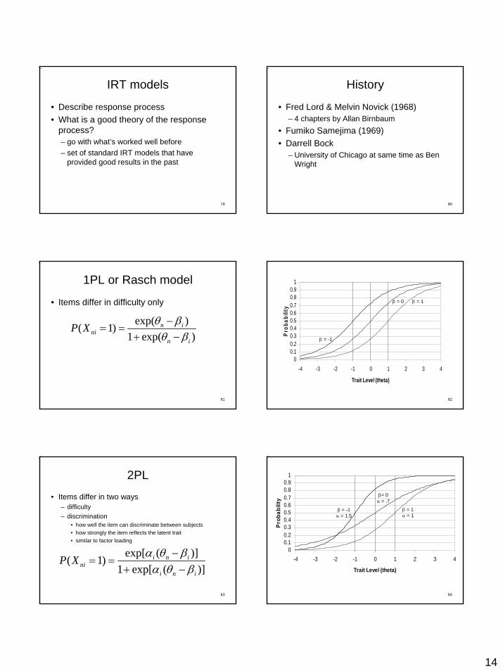
IRT models
• Describe response process• What is a good theory of the response
process?– go with what’s worked well before– set of standard IRT models that have
provided good results in the past
80
History
• Fred Lord & Melvin Novick (1968)– 4 chapters by Allan Birnbaum
• Fumiko Samejima (1969)• Darrell Bock
– University of Chicago at same time as Ben Wright
81
1PL or Rasch model
• Items differ in difficulty only
exp( )( 1)1 exp( )
n ini
n i
P X θ βθ β
−= =
+ −
82
00.10.20.30.40.50.60.70.80.9
1
-4 -3 -2 -1 0 1 2 3 4
Trait Level (theta)
Prob
abili
ty
β = -1
β = 0 β = 1
83
2PL
• Items differ in two ways– difficulty– discrimination
• how well the item can discriminate between subjects • how strongly the item reflects the latent trait• similar to factor loading
exp[ ( )]( 1)1 exp[ ( )]
i n ini
i n i
P X α θ βα θ β
−= =
+ −
84
00.10.20.30.40.50.60.70.80.9
1
-4 -3 -2 -1 0 1 2 3 4
Trait Level (theta)
Prob
abili
ty
β = -1α = 1.5
β= 0α = .7
β = 1α = 1

15
85
3PL
• Items differ in three ways– difficulty– discrimation– guessing or pseudoguessing
• minimal probability of correct response• lower asymptote
exp[ ( )]( 1) (1 )1 exp[ ( )]
i n ini
i n i
P X c c α θ βα θ β
−= = + −
+ −86
00.10.20.30.40.50.60.70.80.9
1
-4 -3 -2 -1 0 1 2 3 4
Trait Level (theta)
Prob
abili
ty β = -1α = 1.5c = 0
β= 0α= .7c = 0 β = 1
α = 1c = .2
87
GSS data
• Bowles, Grimm, & McArdle (in press)• Over 21000 persons from 15 nationally
representative samples– roughly every other year between 1974 and
2000• 10 item multiple choice vocabulary test
– 5 options• Goal: understand relation between age
and vocabulary knowledge88
Item Target Option 1 Option 2 Option 3 Option 4 Option 5WordA Space school noon captain room boardWordB Broaden efface make level elapse embroider widen
WordC Emanate populate free prominent rival come
WordD Edible auspicious eligible fit to eat sagacious able to speak
WordE Animosity hatred animation disobed-ience
diversity friendship
WordF Pact puissance remon-strance
agreement skillet pressure
WordG Cloistered miniature bunched arched malady secluded
WordH Caprice value a star grimace whim induce-ment
WordI Accustom disappoint customary encounter get used business
WordJ Allusion aria illusion eulogy dream reference
89
GSS data
• Winsteps analysis indicated that the test did not fit Rasch model
• Try 2PL and 3PL• Bilog-MG
– dichotomous data– Scientific Software International– ssicentral.com
90
GSS
>GLOBAL DFName = 'gssdkas0.dat', NPArm = 1, LOGistic, SAVe;
>SAVE PARm = 'gss.PAR';>LENGTH NITems = (10);>INPUT NTOtal = 10,
NALt = 2, NIDchar = 1;
>ITEMS INAmes = (word1(1)word10);>TEST1 TNAme = 'TEST0001',
INUmber = (1);(A1,10A1)>CALIB ACCel = 1.0000;
title
1PL (2 for 2PL, 3 for 3PL)
test length
right/wrong
item names
format of data file
16
91
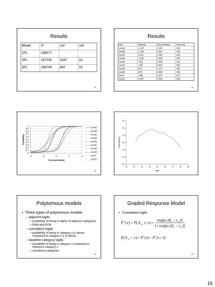
Results
Model X2 ΔX2 Δdf
1PL 189577
2347
487
2PL 187230 10
3PL 186743 10
92
ResultsItem Difficulty Discrimination GuessingwordA -1.137 1.434 .023wordB -1.266 3.554 .016wordC 1.203 1.982 .035wordD -1.281 3.636 .019wordE -.551 2.428 .012wordF -.690 2.659 .030wordG .875 2.172 .092wordH .870 2.839 .060wordI -.908 1.407 .017wordJ 1.043 2.918 .039
93
00.10.20.30.40.50.60.70.80.9
1
-4 -2 0 2 4
Trait level (theta)
Prob
abili
ty
wordA
wordB
wordC
wordDwordE
wordF
wordG
wordH
wordI
wordJ
94Age
10 20 30 40 50 60 70 80 90
Trai
t lev
el ( θ
)
-0.8
-0.6
-0.4
-0.2
0.0
0.2
0.4
95
Polytomous models
• Three types of polytomous models– adjacent logits
• probability of being in higher of adjacent categories• RSM and PCM
– cumulative logits• probability of being in category x or above
compared to category x-1 or below– baseline-category logits
• probability of being in category x compared to reference category z
• unordered categories96
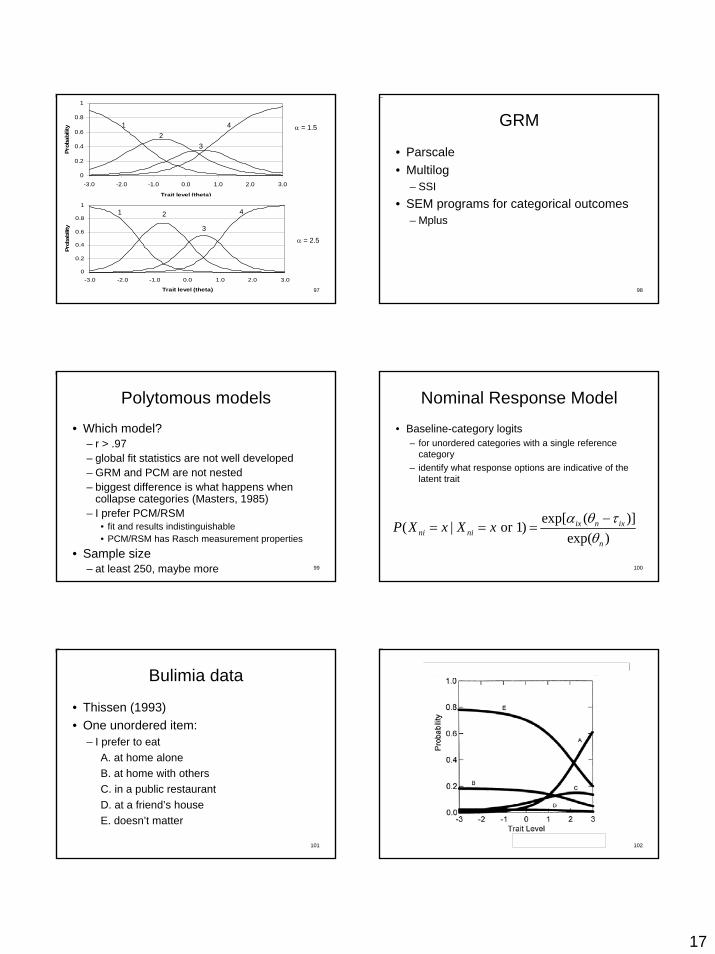
Graded Response Model
• Cumulative logits
* exp[ ( )]( ) ( )1 exp[ ( )]
i n ixni
i n ix
P x P X x α θ τα θ τ
−= ≥ =
+ −
* *( ) ( ) ( 1)niP X x P x P x= = − +
17
97
0
0.2
0.4
0.6
0.8
1
-3.0 -2.0 -1.0 0.0 1.0 2.0 3.0
Trait level (theta)
Prob
abili
ty 12
3
4 α = 1.5
0
0.2
0.4
0.6
0.8
1
-3.0 -2.0 -1.0 0.0 1.0 2.0 3.0
Trait level (theta)
Prob
abili
ty
α = 2.5
1 2
3
4
98
GRM
• Parscale• Multilog
– SSI• SEM programs for categorical outcomes
– Mplus
99
Polytomous models
• Which model?– r > .97– global fit statistics are not well developed– GRM and PCM are not nested– biggest difference is what happens when
collapse categories (Masters, 1985)– I prefer PCM/RSM
• fit and results indistinguishable• PCM/RSM has Rasch measurement properties
• Sample size– at least 250, maybe more 100
Nominal Response Model
• Baseline-category logits– for unordered categories with a single reference
category– identify what response options are indicative of the
latent trait
exp[ ( )]( | or 1)exp( )
ix n ixni ni
n
P X x X x α θ τθ
−= = =
101
Bulimia data
• Thissen (1993)• One unordered item:
– I prefer to eatA. at home aloneB. at home with othersC. in a public restaurantD. at a friend’s houseE. doesn’t matter
102

18
103
Summary
• IRT models are designed to reflect the response process
• Ryan’s opinion: there is little theory in IRT– models are selected because
• they have worked well before• estimation software is available
– little effort to develop response process theory– I call them IRMs- item response models
• Huge advantage over sum scores– item effects are explicitly modeled
104
Advanced topics in IRT
Advantages of explicitly modeling item effects
105
Advanced topics
• Linking• Differential Item Functioning• Computer Adaptive Tests
106
Linking
107
Linking
• How can two tests that measure the same latent trait be linked to the same measurement scale?– same zero point– same measurement unit
108
Linking
• With sum scores, need representative sample– items properties are not part of the model
• cannot be used to link tests– can only use person properties
• only property: sum score• equipercentile equating• regression prediction

19
109
Linking
• Common item equating– items are given on more than one test– assume item parameters are same for both
tests• Common person equating
– persons take multiple items from one or more tests
– assume latent trait level is same for all items
110
Vocabulary data
• McArdle, Grimm, Hamagami, Bowles, & Meredith (2005)
• Goal: understand lifespan development of vocabulary knowledge
• 441 persons from 3 longitudinal studies assessed on tests of intelligence from as young as 3 to as old as age 75
• Problem: tests were not repeated
111
WAIS-RSB-LMSB-L WB-I WAIS WJ-R
SB-LMSB-L WB-I WAIS-R WJ-RWAIS
SB-LMSB-L WB-I WAIS-RWAIS WJ-R
SB-LMSB-L WB-I WJ-RWAIS-RWAIS
SB-LM WB-I WJ-RWAIS-RWAISSB-L
SB-LM WJ-RWAIS-RSB-L WAISWB-I
SB-L WB-I WJ-RWAIS-RWAISSB-LM
SB-L WB-I WJ-RWAIS-RSB-LM WAIS
SB
SB
SB
SB
SB
SB
SB
SB
SB-LM WB-I WJ-RWAIS-RSB-LSB WAIS
SB-LM WB-I WJ-RWAIS-RSB WAISSB-L
SB-M
SB-M
SB-M
SB-M
SB-M
SB-M
SB-M
SB-M
SB-M
SB-M
1.
3.
4.
5.
2.
6.
7.
8.
9.
10.
data file
112
Vocabulary data
• Common item linking– some items are on multiple tests
• for example, WAIS and WAIS-R Vocabulary share 33 items
– tests given in more than one year• Estimated vocabulary knowledge (trait
level) for each person at each measurement occasion– using Rasch model and PCM
113 114

20
115 116
117
Differential Item Functioning
118
DIF
• Does an item work the same for all people?
• Examine if there are differences in item parameters between groups
• May indicate bias– ETS examines tests for evidence of bias
against minorities
119
DIF
1. Force item parameters to be the same in both groups
2. Allow item parameters to vary across groups
3. Compare fit4. Interpret parameter differences
• requires linking assumption between groups
120
WM Span data
• Bowles & Salthouse (2003)• 698 adults• Working memory span (WM span) is the
maximum amount of information that can be stored while engaging in ongoing processing

21
121
Theories• Inhibition deficit
– Hasher & Zacks (1988)• Older adults are less able to suppress
irrelevant information in working memory
• Prediction: older adults should be more susceptible to proactive interference (PI) than younger adults– May, Hasher, & Kane (1999)
• PI will build up faster for older adults 122
Participants
• N = 698• Young
17 <= age <40 N = 280• Middle
40 <= age <60 N = 187• Old
60 <= age <=92 N = 231
123
WM tasks
• Computation Span task– solve arithmetic problem– remember second number in problem
124
READY
125
4 + 2 =a. 3b. 7c. 4d. 6
126
3 + 5 =a. 8b. 6c. 9d. 7

22
127
RECALL
128
Reading span
John read the book in the library.
Who read the book?A. TimB. JohnC. KarenD. Jack
129
WM Span data
• Rasch model• Assume no DIF
– item difficulty same for all three age groups– R2 (age, computation span) = .066 (r = -.26)– R2 (age, reading span) = .099 (r = -.32)
• Allow item difficulty to differ – link by assuming first item has same difficulty
for all three age groups- no PI on first item
130
Computation span
0
2
4
6
8
10
12
14
16
0 1 2 3 4 5 6 7 8 9 10
order position
item
diff
icul
ty
youngmiddleold
131
What’s left?
• Before accounting for differential effects of PI, R2(WM span on age) = .066
• After accounting for differential effects of PI, R2(WM span on age) = .037
• Percent change = 45%
Computation span
132
Reading span
0
2
4
6
8
10
12
14
0 2 4 6 8 10
order position
item
diff
icul
ty
youngmiddleold

23
133
What’s left?
• Before accounting for differential effects of PI, R2(WM span on age) = .099
• After accounting for differential effects of PI, R2(WM span on age) = .043
• Percent change = 57%
Reading span
134
Results
• DIF analysis indicates that about 50% of the age-related variance in WM span is due to differential susceptibility to PI
135
Computer Adaptive Tests
136
Item
Item
Item
Item
Item
Item
Item
Correct
Correct
Correct
Incorrect
Incorrect
Incorrect
137
Advantages
• Tests are targeted (aka tailored)• Greater efficiency
– usually test length cut in half for same precision
• Advantages from computer-administration– e.g. immediate scoring
138
Disadvantages
• Critically dependent on appropriateness of IRT model
• Need large item bank of calibrated items• Scheduling
– GRE and China
24
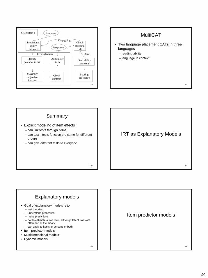
139
Select Item 1 Response
Identify potential items
Maximize objective function
Check controls
Administer item
Item Selection
Response
Provisional ability
estimate
Check stopping
rule
Keep going
Final ability estimate
Done
Scoring procedure
140
MultiCAT
• Two language placement CATs in three languages– reading ability– language in context
141
Summary
• Explicit modeling of item effects– can link tests through items– can test if tests function the same for different
groups– can give different tests to everyone
142
IRT as Explanatory Models
143
Explanatory models• Goal of explanatory models is to
– test theories– understand processes– make predictions– not to estimate a trait level, although latent traits are
often part of the theory– can apply to items or persons or both
• Item predictor models• Multidimensional models• Dynamic models
144
Item predictor models
25
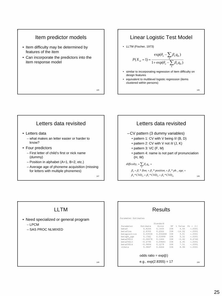
145
Item predictor models
• Item difficulty may be determined by features of the item
• Can incorporate the predictors into the item response model
146
Linear Logistic Test Model• LLTM (Fischer, 1973)
• similar to incorporating regression of item difficulty on design features
• equivalent to multilevel logistic regression (items clustered within persons)
exp( )( 1)
1 exp( )
n k ikk
nin k ik
k
qP X
q
θ β
θ β
−= =
+ −
∑∑
147
Letters data revisited
• Letters data– what makes an letter easier or harder to
know?• Four predictors
– First letter of child’s first or nick name (dummy)
– Position in alphabet (A=1, B=2, etc.)– Average age of phoneme acquisition (missing
for letters with multiple phonemes)148
Letters data revisited
– CV pattern (3 dummy variables)• pattern 1: CV with V being /i/ (B, D)• pattern 2: CV with V not /i/ (J, K)• pattern 3: VC (F, M)• pattern 4: name is not part of pronunciation
(H, W)
0 1 2 3
4 12 5 13 6 14
* * * _ * * *
i k ikk
i i i
difficulty q
flnn position ph ageCVD CVD CVD
β
β β β ββ β β
= =
+ + + +
+ +
∑
149
LLTM
• Need specialized or general program– LPCM– SAS PROC NLMIXED
150
Parameter Estimates
StandardParameter Estimate Error DF t Value Pr > |t|beta0 0.8264 0.1835 338 4.50 <.0001betaflnn 2.8355 0.2022 338 -14.02 <.0001betaposition 0.03534 0.006408 338 5.51 <.0001betaph_age 0.1542 0.02899 338 5.32 <.0001betaCVD12 -0.06078 0.1444 338 -0.42 0.6740betaCVD13 -0.4790 0.09683 338 4.95 <.0001betaCVD14 -0.9604 0.1278 338 7.51 <.0001vtheta 5.9847 0.6664 338 8.98 <.0001
Results
odds ratio = exp(β)
e.g., exp(2.8355) = 17

26
151
Results• 17 times more likely to know the first letter of first or
nickname• 1.03 times more likely to know a letter one position
earlier in the alphabet• 1.17 times more likely to know letter for each half year
earlier that a consonantal phoneme is acquired• No more likely to know a letter containing a consonant
vowel pattern CV not /i/ than a letter containing a consonant vowel pattern CV/i/
• .62 times as likely to know VC than CV/i/• .38 times as likely to know a NOT CV than CV/i/
152
Multidimensional Models
153
Multidimensional models
• Item responses depend on two or more latent traits
• Equivalent to item factor analysis
154
F1 F2
Y1 Y2 Y4 Y5 Y6Y3
155
F1 F2
X1 X2 X4 X5 X6X3
RP1 RP2 RP3 RP4 RP5 RP6
τ1 τ2 τ3 τ4 τ5 τ6
λ11
λ21λ31 λ32
λ42λ52
λ62
τ
10156
Multidimensional models
For one factor model, equivalent to 2PL with– α = λ– β = τ/λ
1
1
exp[ ]( 1)
1 exp[ ]
K
ki kn ik
ni K
ki kn ik
P Xλ θ τ
λ θ τ
=
=
−= =
+ −
∑
∑

27
157
Multidimensional models
• Can do exploratory or confirmatory item factor analysis
• Exploratory– same statistics to decide on number of factors
• scree plot• eigenvalues (of tetrachoric correlation matrix) > 1
– can do rotation to simple structure
158
Multidimensional models
• Estimation (Tate, 2003)• SEM programs
– Mplus– Less robust: Lisrel
• IRT programs– TESTFACT
• Other– NOHARM
159
GSS data
• Goals: – identify whether vocabulary knowledge as
measured by the GSS vocabulary test is unidimensional
– assess relation to age for each dimension• Mplus
160
DimensionsRMSEA: .048 vs. .022
Fit: ΔX2 = 1416, Δdf = 9
161
Item Factor 1loading
Factor 2Loading
Proportioncorrect
worda .703 .003 .78wordb .931 .018 .88wordc .045 .668 .21wordd .894 .051 .88worde .558 .337 .69wordf .565 .356 .74wordg -.022 .705 .32wordh -.025 .796 .28wordi .685 .033 .73wordj .052 .752 .22
162

28
163
Dynamic Models
164
Dynamic models
Incorporate change model into IRT model
Linear change
Exponential learning
exp[ ( , ) ]( 1)1 exp[ ( , ) ]
n itni
n it
f tP Xf t
ββ
Θ −= =
+ Θ −
( , ) *level slopef t tθ θΘ = +
( , ) *exp( * )asymptote startdifference ratef t tθ θ θΘ = + −
165
Emotions data
• Ram, Chow, Bowles, Wang, Grimm, Fujita, & Nesselroade (2005)
• 179 college students• Diaries over 52 days• 16 items
– 8 assessing positive affect– 8 assessing negative affect– 7 point rating scales– item parameters assumed invariant over time
166
Emotions data
• How prevalent is 7-day cycle of emotions?– blue Monday– accounts for 40% of variance in aggregated
data
( , ) t [cos( )] n n n n n ntf t Rμ β ω φ εΘ = + + + +
167
Predicted cycles
168
Results
• Average variance explainedPA: 6.3%NA: 3.0%
– average variance explained for random data: 4%
• Only 77 of 179 show weekly cycle in PA, 44 or 179 in NA
• Phase shift (day of peak) unreliable

29
169
Summary
• IRT can be used not just as a measurement model, but also as an explanatory model
• Three ways– item predictors– multidimensional models– dynamic models
• Can also do– person predictors– item by person interactions
170
Conclusions
171
When to use IRT
• Measurement– validate instruments– choose numbers to assign to subjects
• Explanatory modeling– test theories – make predictions
172
What you need
• Ordered categorical data– except NRM: need baseline category
• Relatively large sample size– I recommend 50 for Rasch model– may need >1000 for complex models
• 3PL• multidimensional
173
Software
• Specialized software– IRT statistics– applicable to only a small number of models– generally not user friendly– error messages incomprehensible– developers helpful and friendly
174
Software
• Generalized software– can do many models– can be painfully slow
• 36 hours for cyclical model– often require programming equations

30
175
IRT Software
Software ModelsWinsteps Rasch, RSM, PCMFacets MRM, Rasch, RSM, PCMBilog-MG 1PL, 2PL, 3PLMultilog GRM, NRM, 1-3PLParscale GRM, RSM, PCM, 1-3PLTestfact MultidimensionalNoharm Multidimensional
176
General Software
Software ModelsMplus 2PL, GRM, MDim, SEMNLMIXED All, but slow and inaccurateWinBUGS All, but slow