Statistical Approaches to Analyzing Well-being DataBy Michael Eid, Free University of Berlin

Citation:Eid, M. (2018). Statistical approaches to analyzing well-being data. In E. Diener, S. Oishi, & L. Tay(Eds.), Handbook of well-being. Salt Lake City, UT: DEF Publishers. DOI:nobascholar.com

Abstract:This chapter gives an overview of modern latent variable models for well-being (WB) research. After ashort introduction into the importance of measurement error and methodological artifacts that can beproduced by measurement error, the basic principles of four types of latent variable models are described:item response theory, latent class analysis, factor analysis, and latent profile analysis. Then, latent variablemodels for multidimensional data structures are discussed and it is shown how the models can be used todefine general WB measures and facet-specific factors. It is pointed out how these models can be applied inmultimethod WB research and how the convergent and discriminant validity can be measured in thiscontext. Finally, a very general model for analyzing variability and change in WB is presented and it isdiscussed how this model and special cases of this model can be applied in WB research.Keywords: latent variable models, item response theory, classical test theory, latent class analysis,latent profile analysis, confirmatory factor analysis, measurement error, g-factor, bifactor model,longitudinal data analysis Over the last decades, there has been an enormous progress in the development of advanced statisticalmethods in the social and behavioral sciences. This chapter will give an overview of some importantmethods that are relevant for well-being (WB) research. It will focus on measurement models that areappropriate for representing the specific characteristics of WB measures. These measurement models canbe used in more complex models to analyze the causes and consequences of WB. As the chapters of this handbook show there are many measures of WB that have been developedover time. If a researcher uses, for example, two different measures in a study, she or he will realize thatthese two measures will not perfectly coincide. It would not be possible to perfectly predict interindividualdifferences in WB on one measure using another. Even if one measures the same individuals repeatedlyusing the same WB measure it is likely that the results are not perfectly the same. To interpret the empiricalresults of WB research appropriately, it is necessary to understand the reasons for the divergence of WBmeasures, to estimate the degree of divergence, and to consider the sources for these degrees of divergence.This can serve to avoid methodological artifacts that could lead to invalid conclusions. There are several reasons why two well-being measures do not perfectly coincide. A first reason ismeasurement error. Whenever we measure something in science we cannot avoid unsystematic influencesthat affect the measurement process. For example, if we weigh ourselves in the morning repeatedly usingthe same balance, the results might differ depending on how we stand on the balance. A second reasonmight be method effects. If one measure is a self-report of WB and the other measure is an observationalmethod the measurements might differ because these assessment methods have peculiarities that are notshared. A third reason can be that the two different WB measures assess different components of WB, forexample, cheerfulness and calmness. A fourth possible reason is that WB has changed between the twomeasurements. In order to separate these different sources of variability in WB scores, measurementmodels are required. This chapter gives an overview of measurement models that can be applied to analyzeWB data, and gives answers to the following questions:

1. Why is it important to consider measurement error?2. How can measurement error be considered?

1

3. How can the multidimensional structure of WB measures be modelled?4. How can method effects be measured?5. How can change in WB be measured?

The approaches presented assume that a random sample is drawn from a population of interest. Insome research contexts, sampling is more complex. One example is cross-cultural WB research in whichrandom samples are taken from different nations. Another example is organizational WB research, inwhich a multilevel sampling process is usual. In a two-level sampling process, for example, firstorganizations (e.g., companies, schools, villages; level-2 units) are drawn from a population oforganizations and then for each organization a random sample of individuals (level-1 units) is selected. Atthe end of this chapter it is discussed how the approaches presented can be extended to these more complexresearch designs.

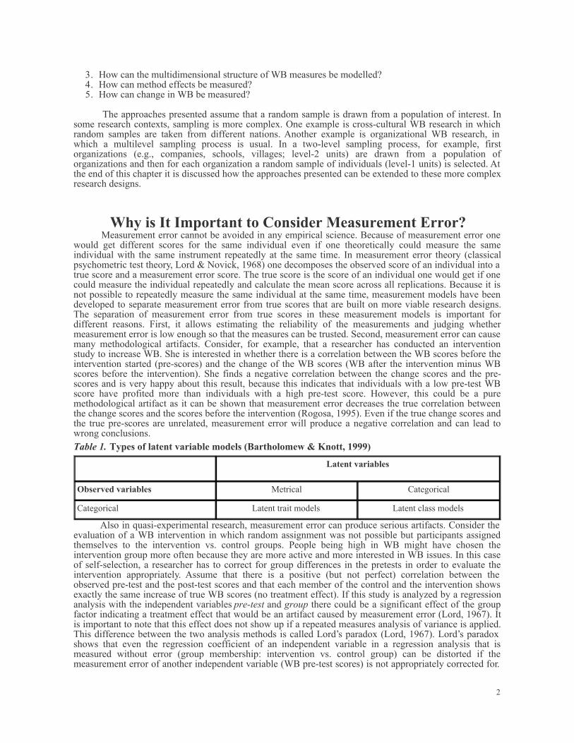
Why is It Important to Consider Measurement Error? Measurement error cannot be avoided in any empirical science. Because of measurement error onewould get different scores for the same individual even if one theoretically could measure the sameindividual with the same instrument repeatedly at the same time. In measurement error theory (classicalpsychometric test theory, Lord & Novick, 1968) one decomposes the observed score of an individual into atrue score and a measurement error score. The true score is the score of an individual one would get if onecould measure the individual repeatedly and calculate the mean score across all replications. Because it isnot possible to repeatedly measure the same individual at the same time, measurement models have beendeveloped to separate measurement error from true scores that are built on more viable research designs.The separation of measurement error from true scores in these measurement models is important fordifferent reasons. First, it allows estimating the reliability of the measurements and judging whethermeasurement error is low enough so that the measures can be trusted. Second, measurement error can causemany methodological artifacts. Consider, for example, that a researcher has conducted an interventionstudy to increase WB. She is interested in whether there is a correlation between the WB scores before theintervention started (pre-scores) and the change of the WB scores (WB after the intervention minus WBscores before the intervention). She finds a negative correlation between the change scores and the pre-scores and is very happy about this result, because this indicates that individuals with a low pre-test WBscore have profited more than individuals with a high pre-test score. However, this could be a puremethodological artifact as it can be shown that measurement error decreases the true correlation betweenthe change scores and the scores before the intervention (Rogosa, 1995). Even if the true change scores andthe true pre-scores are unrelated, measurement error will produce a negative correlation and can lead towrong conclusions.Table 1. Types of latent variable models (Bartholomew & Knott, 1999)

Latent variables

Observed variables Metrical Categorical

Categorical Latent trait models Latent class models

Also in quasi-experimental research, measurement error can produce serious artifacts. Consider theevaluation of a WB intervention in which random assignment was not possible but participants assignedthemselves to the intervention vs. control groups. People being high in WB might have chosen theintervention group more often because they are more active and more interested in WB issues. In this caseof self-selection, a researcher has to correct for group differences in the pretests in order to evaluate theintervention appropriately. Assume that there is a positive (but not perfect) correlation between theobserved pre-test and the post-test scores and that each member of the control and the intervention showsexactly the same increase of true WB scores (no treatment effect). If this study is analyzed by a regressionanalysis with the independent variables pre-test and group there could be a significant effect of the groupfactor indicating a treatment effect that would be an artifact caused by measurement error (Lord, 1967). Itis important to note that this effect does not show up if a repeated measures analysis of variance is applied.This difference between the two analysis methods is called Lord’s paradox (Lord, 1967). Lord’s paradoxshows that even the regression coefficient of an independent variable in a regression analysis that ismeasured without error (group membership: intervention vs. control group) can be distorted if themeasurement error of another independent variable (WB pre-test scores) is not appropriately corrected for.

2

These two examples demonstrate why it is important to correct for measurement error in WB research.

How Can Measurement Error Be Considered?

In order to consider measurement error psychometric models are necessary. In general, four types ofpsychometric models can be distinguished (Bartholomew & Knott, 1999, see Table 1). This distinction isbased on the type of observed variables (categorical vs. metrical) and the types of latent (error-free)variables (categorical vs. metrical). Models with metrical latent variables are dimensional models whereasmodels with categorical latent variables are typological models. In dimensional models, it is assumed thatindividuals as well as items can be ordered on one (or more) continuous variables, whereas this ordering isnot necessary for typological models. The basic ideas of these types of models are explained with respect toone simple representative of each type.Latent Trait Models In Figure 1a the one-parameter logistic test model (also called the Rasch model; Rasch, 1960) isshown. This model is a model for dichotomous observed variables (items) measuring a continuous latentvariable. Consider the (hypothetical) example that participants rated their momentary WB using the threeitems well, cheerful and happy and a two-category response format (no, yes). In the Rasch model, it isassumed that the probability to choose the category yes depends on a value of an individual on acontinuous WB dimension (see Figure 1a). The higher the value of an individual on the WB dimension

3

(latent variable) the higher is the probability to choose the category yes. However, the probability willnever be perfectly 1 (or 0) because of measurement error. Because the probability of the response no is 1minus the probability of the response yes, it is sufficient to consider only one response probability.Individuals differing in their WB will differ in their values on the latent WB variable and can be ordered onthe latent dimensions. These values are not known but can be estimated given their responses to all items.Also, the items can be ordered on the latent dimension according to their difficulty. The item happy inFigure 1a is more difficult than the item well because an individual needs to have a higher value on thelatent WB dimension to obtain a high probability for the category yes than it is the case for the item well.The item cheerful is located on the latent WB between the two other items. An item difficulty parameter isdefined as the value of the latent WB dimension that is linked to a response probability of 0.50. Thesedifficulty parameters are not known but they can be estimated given the response patterns of theparticipants. The Rasch model assumes that the curves describing the response probabilities as functions ofthe latent WB dimension (so-called item characteristic curves) do not differ in their forms between items.Moreover, the model assumes that the latent dimension explains the observed associations (correlations)between the items perfectly (assumption of local independence): The items are correlated because they aremeasuring the same construct (latent variable). Their correlations, however, are not perfect because ofmeasurement error. The assumption that the items are fulfilling the assumptions of a Rasch model can bestatistically tested and there are several ways to relax the assumptions of this model. For example, it can beallowed that the item characteristic curves differ in their steepness by integrating a discrimination parameterin the model (so-called two-parameter logistic model or Birnbaum model; Birnbaum, 1968). Dimensionalmodels for categorical response variables have been extended to more than two response categories. Thereare special models for items with ordered response categories (for an overview, see Nering & Ostini, 2010;Ostini & Nering, 2006). In the partial credit model, for example, there is a probability function for eachcategory of an item (category characteristic curve) that describes the probability to give a response in thiscategory as a function of the latent dimension (Masters, 1982). As the latent dimension is also called latenttrait, this family of models is called latent trait models. Because the item responses are modelled in thesemodels, they are also called models of item response theory. Latent trait model also exist for items withunordered response categories (e.g., nominal scale model; Bock, 1972).Latent Class Models An important property of the model in Figure 1a is that all items and individuals can be ordered onthe same continuum. This implies, for example, that the item happy is more difficult than the item well forall individuals and items. The assumption that all items and all individuals can be ordered on a commonlatent dimension might not be appropriate for all individuals. Consider, for example, the assessment ofdomain life satisfaction with the three items marriage, leisure activities, and job and a dichotomousresponse format (satisfied, dissatisfied). Applying the Rasch model, for example, to these three itemswould require that the three domains are ordered for all individuals in the same way. For example, theordering marriage, leisure activities, and job would imply that all individuals would have a higherprobability to be satisfied with their marriage than with their job or leisure activities. However, there mightbe individuals being happier with their job than their marriage and their leisure activities, and otherconfigurations are possible. In areas of research where it is theoretically and/or empirically not possible toorder items on a dimension in a way that is obligatory for individuals, a typological model with acategorical latent variable is more appropriate. Latent class analysis (LCA) is a typological model forobserved categorical variables (Lazarsfeld & Henry, 1968). In Figure 1b, a (hypothetical) latent class modelfor the three satisfaction items and two latent classes is presented. LCA assumes that the whole populationconsists of subpopulations (latent classes) that differ in the response probabilities for the categories of theobserved items. Each individual of the population has to belong to one, but only one latent class. Thenumber of latent classes is not known but can be estimated given the observed response patterns ofindividuals. The membership of an individual is also not known but the probability of belonging to thedifferent classes can be estimated for each individual (assignment probabilities) and individuals can beassigned to the latent class for which the assignment probability is maximum. All members of the samelatent class show the same response probabilities for the item categories. The members of different latentclasses differ in the profiles of their response probabilities. The latent class structure explains theassociations (correlations) between the observed items perfectly. That means that within each latent classthe items are independent and observed response differences between individuals belonging to the sameclass are due to measurement error. In the model in Figure 1b, the first class is characterized by highprobabilities for being satisfied with marriage and leisure activities and for being dissatisfied with the job.Class 2, on the other hand, is described by high probabilities for being satisfied with the job and dissatisfiedwith marriage and leisure activities. Whether a latent class model fits the data and how many latent classesare necessary can be statistically tested.

4

LCA can be easily extended to items with more than two categories. In the case of multiplecategories, the class-specific response probabilities are estimated for all categories of an item. LCA canalso be applied to items with ordered response categories (e.g., Rost, 1985). An overview of LCA and theirapplications is given by Hagenaars and McCutcheon (2002). Similarities and differences between latentclass and latent trait models are discussed by Heinen (1996). Figures 1a and 1b show important differencesbetween dimensional and typological models. These models have different areas of applications and aresearcher has to decide which type of model is more appropriate for analyzing the research question anddata structure considered.Models of Factor Analysis Models for metrical observed variables are based on the same principal ideas as the models forcategorical observed models. In dimensional models for metrical response variables the item characteristiccurves are not curvilinear such as in latent trait models (see Figure 1a), but linear. In Figure 1c the itemcharacteristic curves for three items and one latent dimension is presented. In this model, the (conditional)expected value of an items is considered as a function of the latent dimension (factor). The deviations ofthe observed values from the item characteristic curves are due to measurement error. The observed values(not shown) scatter around the line (item characteristic curve). The models are called factor analytic modelsor factor models (e.g., Bartholomew & Knott, 1999). These models are applied to metrical variables such asscale scores or response times. The model in Figure 1c is a one-factor model. The straight lines (upper partof Figure 1c) differ in their slopes (factor loadings). In this model, an observed variable is decomposed inone part that is predicted by the latent dimension (factor) and measurement error. The measurement errorvariables are assumed to be uncorrelated. This implies that the factor explains the correlations of theobserved variables perfectly. As in latent trait models, the observed variables (e.g., scales) are correlatedbecause they measure the same construct but they are not perfectly correlated because of measurementerror. Factor analytic models are often depicted as path models (lower part of Figure 1c) in which the latentvariable (factor) is shown as a circle or oval having an influence on the observed variables (squares). Theerror variables are denoted by the letters E.Latent Profile Analysis Typological models for metrical observed variables are called latent profile models (Lazarsfeld &Henry, 1968). Like in LCA it is assumed that the population consists of different subpopulations. Thesubpopulations, however, differ in the profiles of the mean values of the metrical observed variables. If thethree domain satisfaction items were measured on a continuous scale, the result of a latent profile analysiscan look like the result in Figure 1d. The first class is characterized by high expected mean values on theitems marriage and leisure activities and a low expected mean on the item job, whereas it is the other wayaround in Class 2. In classical latent profile analysis, it is assumed that the observed variables are normallydistributed in all latent classes and that the observed variables are independent within latent classes.Other Models The four models presented in Figure 1 are prototypical models. Over the last years, the developmentof psychometric models have made enormous progress and it is possible to extend and to combine thesemodels in different ways. LCA has been combined with other statistical models to detect subpopulationsthat differ in the parameters of a statistical model (so-called mixture distribution models, e. g., Hancock &Samuelsen, 2008). For example, LCA can be combined with latent trait or with factor models to scrutinizewhether there are subpopulations differing in item difficulty parameters or factor loadings. Factor analyticmodels have also been extended in such a way that different types of observed variables (e.g., metrical,ordinal) can be simultaneously analyzed (e. g., Jöreskog & Moustaki, 2001).Computer Programs There are many computer programs available for analyzing latent variable models. There are alsoseveral packages of the computer program R that can be downloaded at no charge from the internet. The Rinternet page Psychometric Models and Methods (https://cran.r-project.org/web/views/Psychometrics.html)gives an overview of currently available R packages for latent variable modeling.

How Can the Multidimensional Structure of WB Measures BeModelled? Well-being is a construct consisting of different components. For example, subjective well-being(SWB) typically comprises the three constructs life satisfaction (LS) , positive affect (PA), and negativeaffect (NA). How distinct are these three constructs? Is it necessary to consider them all in an empiricalstudy? How can their relationships be explained? How can the information that is represented by the threetraits be combined to predict dependent variables such as health and longevity? To scrutinize these

5

important research questions the models presented in Figure 1 have to be extended to multidimensionalmodels. The basic structure of these models will be explained only for metrical observed and latentvariables [models of confirmatory factor analyses (CFA)] but the basic idea of these models can betransferred to other variable types (for multidimensional IRT models see, for example, Deboeck & Wilson,2004; Reckase, 2009; for models of CFA for ordinal variables see, for example, Jöreskog & Moustaki,2001; for multidimensional LCA, see, for example, Hagenaars, 1993).

Figure 2. a) Model with correlated factors; b) Bifactor (S-1) model; c) Bi-factor model; d) Modelwith common independent factor; e) Model with formative well-being factor. Models of confirmatoryfactor analysis for multidimensional data structures. Yik: observed variables, i: indicator, k: facet. λ:loading parameters. Eik: residual (measurement error) variables. LS: life satisfaction, PA: positiveaffect, NA: negative affect, WB: well-being, DV: dependent variable, IV: independent variable, -S:specific factor. In Figure 2a, a multidimensional model with three latent variables (factors) for the three facets ofSWB is depicted. For simplicity, only two observed variables (indicators) for each latent variable (factor)are presented. This model allows for analyzing the latent correlation between the three factors. Thesecorrelations are higher than the correlations between the observed variables because they are not distortedby measurement error. This model allows (a) to test whether the non-perfect correlation between theobserved variables is only due to measurement error or whether the three facets are distinct, (b) to estimatethe degree of discriminant validity [indicated by a (low) correlation coefficient], and (c) whether thedifferent indicators are distinct indicators of the different latent variables (indicated by no cross-loadings).The parameters of the model can be estimated and the goodness-of-fit of this model – as all other models inFigure 2 – can be evaluated by statistical tests and fit indices that have been developed for structuralequation models (SEM; for an overview see Hoyle, 2012; Mulaik, 2009; Schumacker & Lomax, 2010).Several computer programs have been developed for analyzing SEM. One of them is the publicly availableR-package lavaan (Beaujean, 2014; Rosseel, 2012) that can be downloaded at no charge from the internet. If the different components are distinct, researchers are often interested in the specific part of acomponent that is not shared with the other components. Moreover, the causes of these differences can beanalyzed, and it can be investigated whether the components have a unique contribution to predicting andexplaining other dependent variables. There are several ways to define a specific part of a component. Oneway is to select one component as a reference component and to define the specific part of anothercomponent as that part that cannot be predicted by the reference component. This approach is depicted inFigure 2b. In the model in Figure 2b, the latent LS variable is taken as reference factor that predicts allother observed variables. That latent part of PA that cannot be predicted by LS is represented by thespecific factor PA-S that is uncorrelated with the LS factor. The PA-S factor is a residual factor like aresidual in traditional regression analysis and can be interpreted accordingly. It always has a mean of 0. Apositive value of an individual on the PA-S factor indicates that this individual shows a higher PA than one

6

would expect given the LS of this individual. A negative value indicates that the person’s PA is lower thanis expected for a person with this latent LS score. An analog interpretation is true for the specific factorNA-S . The correlation between PA-S and NA-S is a partial correlation. It indicates that part of theassociation between PA-S and NA-S that is not due to LS. The variance explained by the LS factor and thespecific factors can be compared. The proportion of variance of an observed variable by a factor (that isuncorrelated with another one) equals the squared factor loading. The sum of the two squared factorloadings equals the reliability of an observed variable in the model in Figure 1b. The larger the explainedvariance by a specific factor compared to the explained variance by the LS factor the larger is thecomponent specificity. The partial correlation is 0 if LS explains the total correlation between PA-S andNA-S . The model depicted in Figure 2b is called bifactor-( S-1) model and is described in detail by Eid,Geiser, Koch and Heene (2016). If a specific factor had been defined for the indicators of the LS factor in Figure 2b, and if it had beenadditionally assumed that all specific factors are uncorrelated, the model is called bi-factor model (seeFigure 2c; Holzinger & Swineford, 1937). The factor on the left-hand side would then not be the LS factorbut a general factor (G factor). In the case of components of a construct that are not interchangeable, theapplication of the bi-factor model usually produces problematic results and the meaning of the G factor isnot well defined (see Eid et al., 2016, for a deeper discussion). The components of a construct, however,are usually not interchangeable (LS is theoretically a different construct than PA and NA), and, therefore,the bi-factor might not be appropriate for these types of applications. The LS factor and the specific factors in Figure 2b can be correlated with other variables in anextended model (not shown here). They can also be modelled as independent and dependent variables in alatent regression analysis. If specific factors are taken as dependent variables in a regression analysis somearrangements (e.g., transformations) have to be made to avoid methodological artifacts (see Koch,Holtmann, Bohn, & Eid, in press, for a detailed discussion and some guidelines). A second way to define specific factors is to regress all observed variables of SWB on anotherindependent variable (IV) as it is done in Figure 2d. Then, residual factors for all facets of SWB can bedefined indicating that part of a SWB facet that is not predicted by the IV. The values of the specificfactors and their correlations have a similar meaning as in the model presented in Figure 2b. Assume, forexample, that the IV in Figure 2c is flourishing. A positive value of LS-S would then indicate that the LS ofthis person is higher than one expects for a person having such a flourishing score. Also in this model thevariance explained by the IV (flourishing) and by the specific factors can be compared to get a measure ofthe degree of facets specificity. If the facet specificities in Figure 2d were large, this would indicate thatflourishing and SWB are quite different constructs. In some studies, researchers are interested in combing the different facets to a general SWB score topredict a dependent variable (DV) such as health or income. In Figure 2e such a model is presented. In thismodel, the general WB factor is a linear combination of the three facets. This makes it necessary to fix thevariance of the residual of the WB factor in the latent regression to 0. Such a measurement model is called aformative measurement model (e.g., Willoughby, Holochwost, Blanton, & Blair, 2014). An alternative is areflective measurement model of a general WB factor such as the bi-factor model (Figure 2c). To define ageneral WB factor in a formative measurement model it is necessary that there is a dependent variable in themodel that is regressed on the WB factor. Defining a general WB factor in such a formative measurementmodel has several advantages compared to a general factor in the bi-factor model. First, the bi-factor modelcauses many application problems in typical application areas of psychology because it is misspecified forthe construct that are typically considered in multidimensional models (Eid et al., 2016). Second, the WBfactor in Figure 2e is always the best combination of the three facets LS, PA and NA for the DV considered.That means that the meaning of the WB factor changes with changing DV. PA might, for example, having astronger impact on WB than NA when predicting creativity, whereas NA might have a stronger influenceon WB than PA when predicting reasoning tasks. Although formative factors are rare compared to reflectivefactors in psychology, they are promising for future WB research.

How Can Method Effects Be Measured? The most widely used assessment method in research on WB is self-report. WB refers to the innerstate of an individual and the individual is the person that might best know her or his WB. However, areself-reports valid? Are there other assessment methods that provide important information about the WB ofan individual that goes beyond self-report? There are many studies on the validity of self-reports that aresummarized in Chapter 5 of this volume and their results will not be reiterated here. One important strategyin validity research is to apply different methods and to analyze their convergent validity (Campbell &Fiske, 1959). These multimethod studies typically show that there are strong method effects. Methods

7

effects, however, are not the “serpent in the psychologist’s Eden” (Cronbach, 1995, p. 145) but theyrepresent important substantive effects. Validity research typically focus on estimating the convergentvalidity but not on understanding method effects. For example, peer ratings of WB are used to analyzetheir correlation with self-reports but there is less research on the question why peer reports of WB differfrom self-reports. In order to get a deeper understanding of the results of WB research, method effects haveto be understood. How can method effects be analyzed? In recent research on method effects two types oflatent variable models are distinguished that define method effects in a different way (Eid, Geiser, & Koch,2016). These models are the models presented in Figure 2b and Figure 2c for multidimensional datastructures. These models can be applied to multimethod research by replacing the different facets bydifferent methods. The first model (Figure 2b) is appropriate for structurally different methods, whereas thesecond model (Figure 2c) is appropriate for interchangeable methods (Eid, Geiser, & Koch, 2016). Thedifference between these two types of methods can be explained with respect to multiple rater studies.Multiple raters can be considered as multiple methods (Kenny, 1995). Interchangeable raters stem from thesame population of raters, for example, different peers rating a common friend, or different students ratingthe same teacher. Structurally different methods do not stem from the same population. For example, if theWB of a child is measured by a self-report, a parent report and a teacher report, the self, parent, and teacherdo not stem from the same population of interchangeable raters, they have different social roles andexperience the child in quite different contexts. Other examples of structural different methods areobservational methods, physiological measures, reaction time measures, etc. (see Eid et al., 2008; Koch,Eid, & Lochner, in press, for a deeper discussion of these differences and their implications for modelingmultimethod data). In the multimethod model in Figure 2b a reference method (e.g., the child self-report) isselected and contrasted with the other methods (e.g., parent report, teacher report). The method factors havea similar meaning as the facet-specific factors. A method factor represents the over- vs. underestimation oftrait with respect to the value expected based on the reference method (e.g., self-report). The correlationbetween two method factors shows whether two methods have something in common (e.g., common viewof different raters) that is not shared with the reference method. In the multimethod model in Figure 2cthere is a common factor underlying all interchangeable methods. If the three methods considered are, forexample, three peer ratings (three friends of a target) and the peers are randomly assigned to three groups,the general factor measures the expected trait value of a target across all interchangeable raters. Themethod factor represents the deviation of the single raters from the expected values across all raters, thatmeans, it represents the rater-specific view. Because the raters are interchangeable and nested within targetsthe three method factors are uncorrelated (Nussbeck, Eid, Geiser, Courvoisier, & Lischetzke, 2009). In thetwo models presented in Figure 2b und 2c, the variance explained by the factor on the left hand side(squared standardized loadings of the general factor having an influence on all observed variables) is ameasure of convergent validity, whereas the variance explained by the method factors (squaredstandardized method factor loadings) is a measure of method specificity. The general factor and the methodfactors of the models can be related to other variables to explain individual trait differences and methodeffects. The models presented in Figure 2d and 2e can also be applied in multimethod studies in order toexplain the convergence of different methods (Figure 2d) and to combine different methods (e.g., differentraters and/or different physiological variables) for predicting a dependent variable (e.g., health) in anoptimal way (Figure 2e). The multimethod models in Figure 2b and 2c can be extended to multitrait-multimethod (MTMM)models to estimate not only the convergent but also the discriminant validity (see Eid et al., 2008; Koch etal., in press). A guide to more complex multimethod models is given by Eid, Geiser and Koch (2016).MTMM models for ordinal variables are presented by Nussbeck, Eid and Lischetzke (2006), LCA MTMMmodels are discussed by Nussbeck and Eid (2015) as well as Oberski, Hagenaars and Saris (2015).

How Can Change in WB Be Measured? In the analysis of change two general change concepts are considered – variability and change in thenarrow sense (Nesselroade, 1991). Whereas variability refers to reversible short-term fluctuations, changein the narrow sense characterizes change processes that are more long lasting and less reversible(Nesselroade, 1991). The variability of WB measures is often analyzed in a state-trait model of WB.Momentary WB states are considered as fluctuations around a stable WB trait (habitual WB level, set-point,well-being trait, e.g., Eid & Diener, 2004). Several studies have shown that intraindividual variability itselfcan be considered a personality trait as individuals differ in stable way in the variability of their well-beingstates (e.g., Eid & Diener, 1999). Examples of change in the narrow senses are developmental processes and trait changes caused, forexample, by interventions. The variability of WB states is often analyzed in longitudinal studies comprisingmany repeated measurements in a relatively short period. Change processes in the narrow sense are often

8

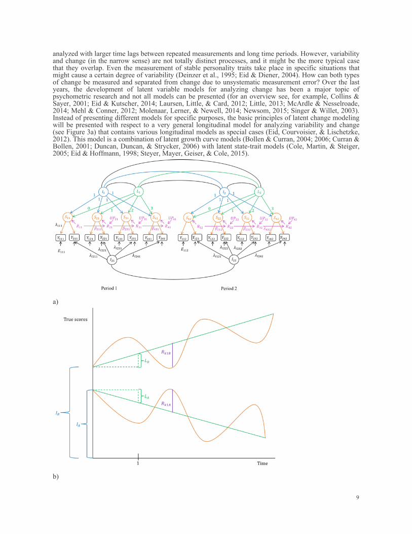
analyzed with larger time lags between repeated measurements and long time periods. However, variabilityand change (in the narrow sense) are not totally distinct processes, and it might be the more typical casethat they overlap. Even the measurement of stable personality traits take place in specific situations thatmight cause a certain degree of variability (Deinzer et al., 1995; Eid & Diener, 2004). How can both typesof change be measured and separated from change due to unsystematic measurement error? Over the lastyears, the development of latent variable models for analyzing change has been a major topic ofpsychometric research and not all models can be presented (for an overview see, for example, Collins &Sayer, 2001; Eid & Kutscher, 2014; Laursen, Little, & Card, 2012; Little, 2013; McArdle & Nesselroade,2014; Mehl & Conner, 2012; Molenaar, Lerner, & Newell, 2014; Newsom, 2015; Singer & Willet, 2003).Instead of presenting different models for specific purposes, the basic principles of latent change modelingwill be presented with respect to a very general longitudinal model for analyzing variability and change(see Figure 3a) that contains various longitudinal models as special cases (Eid, Courvoisier, & Lischetzke,2012). This model is a combination of latent growth curve models (Bollen & Curran, 2004; 2006; Curran &Bollen, 2001; Duncan, Duncan, & Strycker, 2006) with latent state-trait models (Cole, Martin, & Steiger,2005; Eid & Hoffmann, 1998; Steyer, Mayer, Geiser, & Cole, 2015).

a)

b)

9

Figure 3. a) Path model; b) Model for two individuals A and B and one period of time. The colorscorrespond to the colors and variables in figure a). General longitudinal model. Yikp: observed variables, i: indicator, k: occasion of measurement, p:period. λikp, λIikp: loading parameters. Eikp: residual (measurement error variables). Ip: interceptfactor, Lp: slope factor, Skp: latent state variable; Rkp: occasions-specific residual, Ukp: occasion-specifc residual indicating unpredictability. βk(k-1)p: autoregressive parameter. For reasons of claritynot all parameter labels are included. The model presented is a model for two time periods, for example, the periods before and after anintervention or for two days of an experience sampling study. The model can easily be extended to morethan two time periods. Within each time period, there are multiple repeated measurements. For eachoccasion of measurement there are two indicators of a latent state variable Skp characterizing the true WBstate on an occasion of measurement k in a period p. On the level of the latent state variables a latentgrowth curve structure with a linear trend is specified. According to the linear growth model, the statechange of each individual can be characterized by a linear trend. The basic idea of this model for twoindividuals is depicted in Figure 3b. The intercept and the slope of the linear trend can differ betweenindividuals. The individual intercept is a value of the latent intercept factor Ip. The larger the variance ofthis factor, the larger are individual differences in the intercepts. The mean value of the intercept factorrepresents the mean slope of the change process. The individual slopes are values of the slope factor Lp. Alarge variance indicates large differences in the linear trends. The mean value of this factor is the meanslope across all individual slopes. If the variance and the mean of the slope factor are 0, there is no lineartrend in the data and the growth factor can be removed. In this case, the model reduces to a so-called latentstate-trait model with autoregressive effects (Cole et al., 2005; Eid, Holtmann, Santangelo, & Ebner-Priemer, 2017). The intercept factor is then the trait factor characterizing the individual WB level over time.The linear curves do not perfectly determine the change of the state variables because there are residualvariables Rkp. These residuals indicate momentary deviations from the linear trend (or in the case without alinear trend from the latent trait) are due to occasion-specific influences. In addition, there areautoregressive effects on the level of residuals. These effects represent the inertia of the change process(carry-over effects between two neighboring occasions of measurement. To test the hypothesis that theautoregressive process is time homogeneous the autoregressive parameters can be set equal within andbetween periods. Fixing the autoregressive parameters also helps to avoid estimation problems. Theresidual variables (UPkp in Figure 3a) indicate that part of a momentary latent WB state variable that isunpredictable by the intercept and slope factors as well as the state variables measured before. Finally,there is an indicator-specific factor in the model on which the second indicators load. Such a factor is oftennecessary because the two indicators are not perfectly homogenous (unidimensional). Like in themultidimensional model in Figure 2b the number of indicators is one less than the number of indicatorsconsidered (Eid, Schneider, & Schwenkmezger, 1999). If there are more than two indicators and, therefore,more than two indicator factors within a period they can be correlated within and between periods. If theindicators are unidimensional with respect to the latent state variable indicator-specific factors are notnecessary. In the case of unidimensionality the assumption of indicator-specific factors can causeestimation problems (because they are not necessary and do not have substantive variance). Therefore,researchers can start with a model without indicator-specific factors and add them if they are necessarybecause a model without them does not fit the data. Mean stability and mean change between periods can be analyzed with respect to the period-specificintercept and slope factors. For example, after a WB intervention the mean values of the intercept factorcan differ indicating that the intervention might have changed the general WB level. A change of the meanvalues of the slope factor would indicate that the intervention might have changed the developmentalprocess. For WB research, a model without linear change model might be the more typical model becauseof adaptation processes that preclude a linear change. Therefore, stability and change of WB might be wellrepresented by a state-trait model (Eid & Diener, 2004).Measurement Invariance In longitudinal studies, different types of measurement invariance over time can be considered(Millsap, 2011). Measurement invariance (MI) concerns the question whether the same WB states aremeasured or whether there is a structural change in the link between the latent and observed variablesshowing that the psychometric meaning of the WB measures has changed. The lowest level of MI isconfigural invariance. That means that the number of latent variables do not differ between occasions ofmeasurement and time periods. Weak MI additionally assumes that the values of the loading parameters of

10

the latent variables do not differ between occasions of measurement and time periods. Weak MI isnecessary if one wants to relate the latent variables to other variables in extended models and to make surethat the structurally the same WB factors are measured on each occasion of measurement. Strong MIadditionally requires that the intercepts of an observed variable do not change over time. The intercepts arenot shown in the path models presented in this chapter. Intercepts are additional constants that are specificto an observed variable and mainly determine the mean value of the observed variables. Strong MI isrequired when one wants to compare latent means over time, e.g., the means of the intercept factors beforeand after an intervention. If strong MI is not given this would indicate that mean change was indicatorspecific and is not well-captured by the means of the latent variables. Strict MI would additionally assumethat the variances of the error variables do not change over time. This is not required for relating latentvariables to other variables or testing for mean differences but it is interesting to see whether the quality ofWB measurements changes over time. Often it is also assumed that the autoregressive process is time-invariant with non-changing autoregressive parameters and residuals of the UP variables over time. The measurement model that is shown for one construct in Figure 3a can be extended by includingother variables. For example, if there are multiple constructs, a measurement model can be specified foreach construct and the mutual influences of the variables over time can be analyzed (e.g., Wickrama, Lee,O’Neal, & Lorenz, 2016). The model in Figure 3 assumes that the time lag between the occasions ofmeasurements is the same between all occasions and for all individuals. This assumption might be violated,for example, in experience sampling studies in which occasions of measurements are individually selected.In such studies, the loadings of the intercepts and the autoregressive parameters have to consider theseindividual differences in time lags (Eid et al., 2012). This can be done, for example, in the context ofdynamic structural equation modeling (Driver, Oud, & Voelkle, 2017; Asparouhov, Hamaker, & Muthen,2017).

How Can These Models Be Extended to Analyze MultipleGroups? The models presented assume that a sample of individuals was randomly drawn from a population.In WB research, the sampling process is sometimes more complex. Often, it is of interest to analyzedifferent groups, for example, nations, intervention groups, schools, companies, etc. There are two ways toconsider group differences – multigroup and multilevel analysis. In multigroup analyses different groupsare selected because the researcher is interested in exactly these groups. In a replication of a study, aresearcher would select samples exactly from the same groups. For example, the researcher might beinterested in comparing women and men, China and the US, or an intervention with a control group. In thiscase, multigroup analysis is appropriate. In multigroup analysis a latent variable model is specified in eachgroup and several hypotheses about between group differences with respect to the parameters of a model(e.g., factorial structure, mean differences, regression parameters) can be tested. The models considered inthis chapter can be easily extended to multigroup analysis (e.g., Bock & Zimowski, 1997; Brown, 2015;Eid, Langeheine, & Diener, 2003). If there are many groups testing assumptions across groups (e.g., testingmeasurement invariance across many nations) can become very cumbersome. In this case, recentdevelopments of methods for analyzing many groups can be applied (for an overview and comparison ofdifferent approaches see Kim, Cao, Wang, & Nguyen, 2017). In multilevel analysis, it is assumed that the groups themselves are randomly selected from apopulation of groups. For example, a WB researcher might be interested in work satisfaction and randomlyselect different companies (level-2 units) and employees within companies (level 1 units). The level-2units are considered interchangeable. In a replication of such a study, the researcher would get a differentsample of level-2 units. Like in multigroup analysis, the level-2 units can differ in the parameters of amodel. In addition to multigroup analysis, however, the variations of the parameters between groups can beexplained by other variables. Because the level-2 units are randomly selected, the parameters of the modelhave a distribution. It can be estimated how strong the variation of parameters is and to which degree level-2 differences in the parameters can be predicted by other level-2 variables (e.g., the organizational climateof a company). Multilevel extensions have been developed for the different types of psychometric modelsin Table 1 (e.g., Adams, Wilson, & Wu, 1997; Heck & Thomas, 2015; Skrondal & Rabe-Hesketh, 2014;Tay, Diener, Drasgow, & Vermunt, 2011; Vermunt, 2003; 2008). Multigroup and multilevel analyses require that the group membership of an individual is known. If aresearcher has the hypothesis that the parameter of a model differ between subgroups but the subgroups arenot known, latent class analysis can be combined with the models presented so far resulting in mixturedistribution models (e.g., Hancock & Samuelsen, 2008). For example, latent variable models oflongitudinal research can be extended to latent growth mixture models (Wickrama et al., 2016) or mixture

11

distribution latent state-trait models (Courvoisier, Eid, & Nussbeck, 2007) to detect populationheterogeneity with respect to the change process (e.g. degree of variability, mean growth rates).

Conclusion Latent variable models enable the estimation of unsystematic measurement error from systematicsources of WB differences. This allows avoiding methodological artifacts and estimation biases that arecaused by measurement error. They also enable researcher testing theories about the measurement of WB aswell as its causes and consequences in a sophisticated way. Latent variable models have been developedfor different areas of application and can be combined and extended in manifold ways to fulfill the needs ofempirical WB research.

ReferencesAdams, R. J., Wilson, M., & Wu, M. (1997). Multilevel item response models: An approach to errors invariable regression. Journal of Educational and Behavioral Statistics, 22 , 47-76.Asparouhov, T., Hamaker, E.L., & Muthen, B. (2017). Dynamic structural equation models. TechnicalReport. Version 2. Los Angeles: Muthén & Muthén.Bartholomew, D.J. & Knott, M. (1999). Latent variable models and factor analysis . London: Arnold.Beaujean, A. A. (2014). Latent variable modeling using R. New York: Routledge.Birnbaum, A. (1968). Some latent trait models and their use in inferring an examinee’s ability. In F.M.Lord & M. R. Novick (Eds.), Statistical theories of mental test scores (pp. 395-479). Reading, MA:Addison-Wesley.Bock, R. D. (1972). Estimating item parameters and latent ability when responses are scored in two or morenominal categories. Psychometrika, 37, 29-51.Bock, R. D. & Zimowski, M. F. (1997). Multiple group IRT. In W.J. van der Linden & Ronald K.Hambleton (Eds.), Handbook of item response theory (pp. 433-448). New York: Springer-Verlag.Bollen, K. A. & Curran, P. J. (2004). Autoregressive latent trajectory (ALT) models: A synthesis of twotraditions. Sociological Methods & Research, 32 , 336-383.Bollen, K. A. & Curran, P. J. (2006). Latent curve models: A structural equation perspective. New York:Wiley.Brown, T. A. (2015). Confirmatory factor analysis for applied research . New York, NY: Guilford Press.Campbell, D. T., & Fiske, D. W. (1959). Convergent and disciminant validation by the multitrait-multimethod matrix. Psychological Bulletin, 56, 81-105.Cole, D. A., Martin, N. C., & Steiger, J. H. (2005). Empirical and conceptual problems with longitudinaltrait-state models: Introducing a trait-state-occasion model. Psychological Methods, 10, 3-20.Collins, L. M. & Sayer, A. G. (Eds.). (2001). New methods for the analysis of change . Washington, DC:American Psychological Association.Courvoisier, D., Eid, M., & Nussbeck, F. W. (2007). Mixture distribution state-trait models. PsychologicalMethods, 12, 80-104.Cronbach, L. J. (1995). Giving method variance its due. In P. E. Shrout & S. T. Fiske (Eds.), Personalityresearch, methods, and theory: A festschrift honoring Donald W. Fiske (pp. 145-160). Hillsdale, NJ:Erlbaum.Curran, P. J. & Bollen, K. A. (2001). The best of both worlds: Combining autoregressive and latent curvemodels. In Collins, L. M. & Sayer, A. G. (Eds.), New methods for the analysis of change (pp.105-136).Washington, DC: American Psychological Association.Deboeck, P. & Wilson, M. (Eds.). (2004). Explanatory item response models: A generalized linear andnonlinear approach. New York: Springer.Deinzer, R., Steyer, R., Eid, M., Notz, P., Schwenkmezger, P., Ostendorf, F., & Neubauer, A. (1995).Situational effects in trait assessment: The FPI, NEOFFI and EPI Questionnaires. European Journal ofPersonality, 9, 1-23.Driver, C. C., Oud, J. H. L., & Voelkle, M. C. (2017). Continuous time structural equation modeling with Rpackage ctsem. Journal of Statistical Software , 77, 1-35.Duncan, T. E., Duncan, S. C., & Strycker, L. A. (2006). An introduction to latent variable growth curve

12

modeling: Concepts, issues, and applications (2nd ed.). Mahwah, NJ: Lawrence Erlbaum.Eid, M., Courvoisier, D. S., & Lischetzke, T. (2012). Structural equation modeling of ambulatoryassessment data. In M. R. Mehl & T.S. Connor (Eds.), Handbook of research methods for studying dailylife (pp. 384-406). New York: Guilford.Eid, M. & Diener, E. (1999). Intraindividual variability in affect: Reliability, validity, and personalitycorrelates. Journal of Personality and Social Psychology, 76, 662-676.Eid, M. & Diener, E. (2004). Global judgments of subjective well-being: Situational variability and long-term stability. Social Indicators Research, 65, 245-277.Eid, M., Geiser, C., & Koch, T. (2016). Measuring method effects: From traditional to design-orientedapproaches. Current Directions in Psychological Science 25 , 275-280.Eid, M., Geiser, C., Koch, T., & Heene, M. (2016, August 15). Anomalous results in G-factor models:Explanations and alternatives. Psychological Methods. Advance online publication.Eid, M. & Hoffmann, L. (1998). Measuring variability and change with an item response model forpolytomous variables. Journal of Educational and Behavioral Statistics , 23, 193-215.Eid, M., Holtmann, J., Santangelo, P., & Ebner-Priemer, U. (2017). On the definition of latent state-traitmodels with autoregressive effects: Insights from LST-R theory. European Journal of PsychologicalAssessment, 33, 285-295.Eid, M. & Kutscher, T. (2014). Statistical models for analyzing stability and change in happiness. In K. M.Sheldon & R. E. Lucas (Eds.), Stability of happiness: Theories and evidence on whether happiness canchange (pp. 263-297). Amsterdam: Elsevier.Eid, M., Langeheine, R., & Diener, E. (2003). Comparing typological structures across cultures by latentclass analysis: A primer. Journal of Cross-Cultural Psychology, 34,195-210.Eid, M., Nussbeck, F. W., Geiser, C., Cole, D. A., Gollwitzer, M., & Lischetzke, T. (2008). Structuralequation modeling of multitrait-multimethod data: Different models for different types of methods.Psychological Methods, 13, 230-253.Eid, M., Schneider, C., & Schwenkmezger, P. (1999). Do you feel better or worse? On the validity ofperceived deviations of mood states from mood traits. European Journal of Personality, 13, 283-306.Hagenaars, J. A. (1993). Loglinear models with latent variables. Newbury Park: Sage.Hagenaars, J. A., & McCutcheon, A. L. (2002). Applied latent class analysis. New York: CambridgeUniversity Press.Hancock, G. R. & Samuelsen, K. M. (2008). Advances in latent variable mixture models. Charlotte, NC:Information Age Publishing.Heck, R. H. & Thomas, S. L. (2015). An introduction to multilevel modeling techniques. MLM and SEMapproaches using Mplus. New York: Routledge.Heinen, T. (1996). Latent class and discrete latent trait models: Similarities and differences. ThousandOaks, California: Sage.Holzinger, K. & Swineford, F. (1937). The bi-factor method. Psychometrika, 2, 41-54.

Hoyle, R. H. (Ed.) (2012). Structural equation modeling. Concepts, issues, and applications (2 nd ed.).Thousands Oaks: Sage.Jöreskog, K. G. & Moustaki, I. (2001). Factor analysis of ordinal variables: A comparison of threeapproaches. Multivariate Behavioral Research, 36, 347-387.Kenny, D. A. (1995). The multitrait-multimethod matrix: Design, analysis, and conceptual issues. In P.E.Shrout & S. T. Fiske (Eds.), Personality research, methods, and theory: A festschrift honoring Donald W.Fiske (pp.111-124). Hillsdale, NJ: Lawrence Erlbaum Associates.Kim, E. S., Cao, C., Wang, Y., & Nguyen, D. T. (2017) Measurement invariance testing with many groups:A comparison of five approaches. Structural Equation Modeling, 24, 524-544Koch, T., Eid, M., & Lochner, K. (in press). Multitrait-multimethod-analysis: The psychometric foundationof CFA-MTMM models. In P. Irwing, T. Booth & D. Hughes (Eds.), The Wiley handbook of psychometrictesting. London: John Wiley & Sons.Koch, T., Holtmann, J., Bohn, J., & Eid, M. (in press). Explaining general and specific factors inlongitudinal, multimethod, and bi-factor models: Some caveats and recommendations. PsychologicalMethods.

13

Laursen, B., Little, T. D., & Card, N. A. (Eds.) (2012). Handbook of developmental research methods. NewYork: Guilford.Lazarsfeld, P. F. & Henry, N. W. (1968). Latent structure analysis. Boston: Houghton Mifflin.Little, T. D. (Ed. ) (2013). Longitudinal structural equation modeling. New York: The Guilford Press.Lord, F. M. (1967). A paradox in the interpretation of group comparisons. Psychological Bulletin, 68, 304–305.Lord, F. M. & Novick, M. R. (1968). Statistical theories of mental test scores . Reading, MA: Addison-Wesley.Masters, G. N. (1982). A Rasch model for partial credit scoring. Psychometrika, 47, 149-174.McArdle, J. J. & Nesselroade, J. R. (Eds.) (2014). Longitudinal data analysis using structural equationmodels. Washington, DC: American Psychological Association.Mehl, M. R. & Conner, T. S. (Eds.) (2012). Handbook of research methods for studying daily life . NewYork: The Guilford Press.Millsap, R. E. (Ed.) (2011). Statistical approaches to measurement invariance . New York: Routledge,Taylor, & Francis Group.Molenaar, P. C. M., Lerner, R. M., & Newell, K. M: (Eds.) (2014). Handbook of developmental systemstheory and methodology. New York: The Guilford Press.Mulaik, S. A. (2009). Linear causal modeling with structural equations . Boca Raton: CRC Press.Nering, M. L. & Ostini, R. (Eds.) (2010). Handbook of polytomous item response theory models. NewYork: Routledge.Nesselroade, J. R. (1991). Interindividual differences in intraindividual changes. In L. M. Collins & J.L.Horn (Eds.), Best methods for the analysis of change: Recent advances, unanswered questions, futuredirections (pp. 92-105). Washington, DC: American Psychological Association.Newsom, J. T. (2015). Longitudinal structural equation modeling. A comprehensive introduction. NewYork: Routledge.Nussbeck, F.W., & Eid, M. (2015). Multimethod latent class analysis. Frontiers in Psychology , 6, Article1332.Nussbeck, F. W., Eid, M., Geiser, C., Courvoisier, D. S., & Lischetzke, T. (2009). A CTC(M–1) model fordifferent types of raters. Methodology, 5, 88-98.Nussbeck, F. W., Eid, M., & Lischetzke, T. (2006). Analyzing MTMM data with SEM for ordinal variablesapplying the WLSMV-estimator: What is the sample size needed for valid results? British Journal ofMathematical and Statistical Psychology, 59, 195-213.Oberski, D. L., Hagenaars, J. A., & Saris, W. E. (2015). The latent class multitrait-multimethod model.Psychological Methods, 20, 422-443.Ostini, R. & Nering, M. L. (2006). Polytomous item response theory models . Thousand Oaks: Sage.Rasch, G. (1960). Probabilistic models for some intelligence and attainment tests . Copenhagen: Nielsen &Lydiche.Reckase, M. D. (2009). Multidimensional item response theory. Dordrecht: Springer.Rogosa, D. R. (1995). Myths and methods: "Myths about longitudinal research," plus supplementalquestions. In J. M. Gottman (Ed.), The analysis of change (pp. 3-65). Hillsdale, New Jersey: LawrenceErlbaum Associates.Rosseel, Y. (2012). Lavaan: An R package for structural equation modeling. Journal of StatisticalSoftware, 48, 1-36.Rost, J. (1985). A latent class model for rating data. Psychometrika, 50, 37-49.Schumacker, R. E. & Lomax, R. G. (2010). A beginner’s guide to structural equation modelling (3nd ed.)Mahwah: Erlbaum.Singer, J. D. & Willet, J. B. (2003). Applied longitudinal data analysis . London: Oxford University Press.Skrondal, A. & Rabe-Hesketh, S. (2014). Generalized latent variable modeling: Multilevel, longitudinaland structural equation models (2nd ed.). Boca Raton, FL: Chapman & Hall.Steyer, R., Mayer, A., Geiser, C., & Cole, D. A. (2015). A theory of states and traits - revised. Annual

14

Review of Clinical Psychology, 11, 71-98.Tay, L., Diener, E., Drasgow, F., & Vermunt, J. K. (2011). Multilevel mixed-measurement IRT analysis:An explication and application to self-reported emotions around the world. Organizational ResearchMethods, 14, 177-207.Vermunt, J.K. (2003) Multilevel latent class models. Sociological Methodology, 33, 213-239.Vermunt, J.K. (2008). Latent class and finite mixture models for multilevel data sets. Statistical Methods inMedical Research, 17, 33-51.Wickrama, K. A. S., Lee, T. K., O’Neal, C. W., & Lorenz, F. O. (2016). Higher-order growth curves andmixture modeling with Mplus. New York: Routledge.Willoughby, M., Holochwost, S.J., Blanton, Z.E., & Blair, C.B. (2014). Executive functions: Formativeversus reflective measurement. Measurement: Interdisciplinary Research and Perspectives , 12, 69-95.

2018 Ed Diener. Copyright Creative Commons: Attribution, noncommercial, noderivatives

15