measurement of slip velocity and lift coefficient for

Clemson UniversityTigerPrints

All Theses Theses

8-2016

Measurement of Slip Velocity and Lift Coefficientfor Laterally Focused Particles in an Inertial Flowthrough a Spiral Microfluidic ChannelSaurabh Satish DeshpandeClemson University, [email protected]

Follow this and additional works at: https://tigerprints.clemson.edu/all_theses

This Thesis is brought to you for free and open access by the Theses at TigerPrints. It has been accepted for inclusion in All Theses by an authorizedadministrator of TigerPrints. For more information, please contact [email protected].

Recommended CitationDeshpande, Saurabh Satish, "Measurement of Slip Velocity and Lift Coefficient for Laterally Focused Particles in an Inertial Flowthrough a Spiral Microfluidic Channel" (2016). All Theses. 2477.https://tigerprints.clemson.edu/all_theses/2477

https://tigerprints.clemson.edu?utm_source=tigerprints.clemson.edu%2Fall_theses%2F2477&utm_medium=PDF&utm_campaign=PDFCoverPages

https://tigerprints.clemson.edu/all_theses?utm_source=tigerprints.clemson.edu%2Fall_theses%2F2477&utm_medium=PDF&utm_campaign=PDFCoverPages

https://tigerprints.clemson.edu/theses?utm_source=tigerprints.clemson.edu%2Fall_theses%2F2477&utm_medium=PDF&utm_campaign=PDFCoverPages

https://tigerprints.clemson.edu/all_theses?utm_source=tigerprints.clemson.edu%2Fall_theses%2F2477&utm_medium=PDF&utm_campaign=PDFCoverPages

https://tigerprints.clemson.edu/all_theses/2477?utm_source=tigerprints.clemson.edu%2Fall_theses%2F2477&utm_medium=PDF&utm_campaign=PDFCoverPages

mailto:[email protected]

MEASUREMENT OF SLIP VELOCITY AND LIFT COEFFICIENT FOR LATERALLY FOCUSED PARTICLES

IN AN INERTIAL FLOW THROUGH A SPIRAL MICROFLUIDIC CHANNEL

A Thesis

Presented to

the Graduate School of

Clemson University

In Partial Fulfillment

of the Requirements for the Degree

Master of Science

Mechanical Engineering

by

Saurabh Satish Deshpande

August 2016

Accepted by:

Dr. Phanindra Tallapragada, Committee Chair

Dr. Xiangchun Xuan

Dr. Melur Ramasubramanian

ii

ABSTRACT

Microfluidic channels with a spiral geometry are extensively researched for their use in particle

focusing, separation and identification. Instead of using electrophoresis, magnetophoresis, etc.,

spiral channel takes advantage of the Inertial Lift Force along with the Viscous Drag to achieve

size based separation of particles. Inertial microfluidic channel can have high throughput and are

much safer to use for live cell separation and other physiological fluids processing.

A particle flowing freely in a spiral microchannel at low Reynolds number inertial flow, attains

lateral equilibrium due to balance of Inertial Lift force and the viscous Dean Drag. The inertial lift

forces are primarily due to the wall effect and the shear gradient of the fluid flow profile. Much

theoretical research has been done in this field to explain the lateral migration of a particle in an

inertial fluid flow. Notable contributions were made by Saffman (1965), Ho and Leal (1974) and

later Vasseur and Cox (1976) in explaining the lift force on a particle theoretically. All these and

many other theoretical models developed in the last few decades discuss Lift force being

dependent on the particle slip velocity. Additionally many models including the one developed by

Saffman predicts a linear dependence of Lift force on the slip velocity of particle. But it seems that

the microfluidic community has ignored this dependence with the result that several hypotheses

and models exist in which the slip velocity is nonexistent.

The measurement of slip velocities for particles has never been done in the field of microfluidics.

The current study aims to do so and bridge the gap in understanding the Lift force responsible for

the lateral migration of particles. The focused particle’s velocity when it passes through the outer

arm of the spiral microfluidic device is measured experimentally followed by a computational

iii

study (using COMSOL Multiphysics) to obtain the undisturbed fluid flow velocity through the spiral

arm.

To calculate the slip velocity, identification of focusing positions in the horizontal and vertical

plane of the channel is necessary. Identification in horizontal plane is easy by simply observing

the channel under microscope. To identify the vertical focusing positions, a high speed camera

(Photron SA-4) coupled with a Nikon microscope and a 50x objective lens (depth of focus = 0.9

um) is used. The narrow depth of focus of objective lens coupled with the precise movement of

microfluidic device in the vertical plane is used to identify the height of focused particles from the

channel bottom. A focus-measure of all the acquired images is calculated (using a Matlab script

which calculates the global variance of an image as a focus-measure) followed by its statistical

distribution to obtain the particle’s vertical location within an error of ±5 um. Velocity of the

particles for all the focused positions is now calculated using a Matlab script which detects the

particles from the acquired images and traces it across successive frames.

At the focused position, particle is in equilibrium due to a balance of Dean Drag and the Inertial

Lift force. Velocity components of Dean Flow are obtained from the computational study,

followed by calculation of Dean Drag acting on the focused particles. The Lift force acting on the

particle is now known and equating it with the slip velocity of particles, numerical values of Lift

coefficient are obtained for the first time. These Lift coefficients are obtained for various focusing

positions in the vertical plane of channel for two sets of Reynolds number.

iv

Dedicated to my Parents

v

ACKNOWLEDGMENTS

I want to thank my advisor Dr. Tallapragada Phanindra for having faith in me and believing in me

for the past one and half years. I would not have been able to complete my M.S. and this Thesis

without his support and aid.

Next, I want to thank Dr. Xuan from Mechanical Engineering Department at Clemson University

for allowing me to fabricate microfluidic devices at his Lab. I also want to thank Mr. Bill Delaney

from Advanced Material Research Laboratory at Clemson University for helping me with his

extensive experience in fabricating microfluidic devices and allowing me to work at AMRL’s Clean

room facility.

I want to thank my Mother, Swati Deshpande, my Father, Satish Deshpande and my Fiancé, Aditi

Khanorkar, for morally supporting me during my Graduate studies. Last, I want to thank my

friends, Shyamal Satodia and Aditya Dabral who have helped me through the tough times of my

stay at Clemson.

vi

TABLE OF CONTENTS

Page

TITLE PAGE ......................................................................................................................................... i

ABSTRACT ......................................................................................................................................... ii

DEDICATION .................................................................................................................................... iv

ACKNOWLEDGEMENTS .................................................................................................................... v

LIST OF PLOTS ............................................................................................................................... viiii

LIST OF FIGURE ................................................................................................................................ xi

LIST OF TABLE ................................................................................................................................ xiii

CHAPTER 1. LITERATURE REVIEW ................................................................................................ 1

1.1 BRIEF HISTORY OF INERTIAL FOCUSING AND LATERAL MIGRATION OF PARTICLES ........ 1

1.2 INERTIAL MICROFLUIDICS ................................................................................................. 2

1.3 FORCES ACTING ON A SPHERICAL PARTICLE .................................................................... 3

1.4 IMPORTANCE OF PARTICLE SLIP VELOCITY ....................................................................... 6

1.5 STRUCTURE OF THESIS ...................................................................................................... 7

CHAPTER 2. EXPERIMENTAL SETUP ............................................................................................. 9

2.1 DESIGN OF MICROFLUIDIC CHANNEL ............................................................................... 9

2.2 FABRICATION OF MOLD AND PDMS DEVICE .................................................................. 10

vii

Table of Contents (Continued)

Page

2.3 PREPARATION OF PARTICLE SOLUTION .......................................................................... 11

2.4 MICROSCOPE SETUP ....................................................................................................... 12

2.5 EXPERIMENTAL PROCEDURE .......................................................................................... 13

CHAPTER 3. DATA COLLECTION AND DATA ANALYSIS .............................................................. 14

3.1 INTRODUCTION ............................................................................................................... 14

3.2 MEASUREMENT OF OBJECT’S HEIGHT USING MICROSCOPE ......................................... 15

3.3 RELATIONSHIP BETWEEN Z-STAGE MOVEMENT AND THE FOCAL PLANE MOVEMENT . 16

3.4 IDENTIFICATION OF FOCUSING POSITIONS IN VERTICAL PLANE .................................... 20

3.5 USE OF FOCUS MEASURE TO VERIFY THE PARTICLES POSITION IN VERTICAL PLANE .... 28

3.6 CALCULATION OF PARTICLE VELOCITY ........................................................................... 32

3.7 SPREAD OF PARTICLES INSIDE THE CHANNEL AND ESTIMATION OF ERROR ................. 35

3.8 UNDISTURBED FLUID FLOW VELOCITY ........................................................................... 36

CHAPTER 4. RESULTS AND DISCUSSION: SLIP VELOCITY AND LIFT COEFFICIENT ...................... 42

4.1 SLIP VELOCITY OF 24 µM PARTICLES AT RE = 13.7 AND 17.2 ......................................... 42

4.2 LIFT COEFFICIENTS OF 24 µM PARTICLES AT RE=13.7 AND 17.2 .................................... 49

4.3 DISCUSSION OF RESULTS ................................................................................................ 65

CHAPTER 5. CONCLUSION AND FUTURE WORK ........................................................................ 69

viii

Table of Contents (Continued)

Page

APPENDICES ................................................................................................................................... 71

APPENDIX A SOFT LITHOGRAPHY PROCEDURE .............................................................. 72

APPENDIX B RELATIONSHIP BETWEEN STAGE MOVEMENT AND FOCUSING PLANE ..... 74

APPENDIX C MATLAB SCRIPT FORGVFM OF AN IMAGE ................................................. 77

APPENDIX D MATLAB SCRIPT FOR CALCULATION OF PARTICLE VELOCITY .................... 80

REFERENCES .................................................................................................................................. 83

ix

LIST OF PLOTS

Page

Plot 3.1 GVFM histogram at 20 um z-stage height ........................................................................ 30

Plot 3.2 GVFM of particles vs z-stage movement.......................................................................... 31

Plot 3.3 GVFM value vs z-stage movement for channel bottom detection .................................. 32

Plot 3.4 Particle velocity vs particle distance from inner wall....................................................... 35

Plot 3.5 Range of particle velocity and undisturbed fluid velocity ................................................ 39

Plot 3.6 Average particle velocity and Fluid velocity ..................................................................... 40

Plot 3.7 Slip velocity ...................................................................................................................... 40

Plot 4.1Particle velocity plot, Re=13.7, Vertical focus position of 22 um ..................................... 43

Plot 4.2 Particle velocity plot, Re=13.7, Vertical focus position of 67 um .................................... 43

Plot 4.3 Range of particle velocity, Re=13.7, Vertical focus position of 22 um............................. 44


Plot 4.5 Slip velocity of particle 22 um above channel bottom, Re=13.7 ..................................... 45

Plot 4.6 Slip velocity of particle 67 um above channel bottom, Re=13.7 ..................................... 45

Plot 4.7 Particle velocity, Re= 17.2, Vertical focus position of 15 um ........................................... 46

Plot 4.8 particle velocity, Re=17.2, Vertical focus position of 67 um ............................................ 46


Plot 4.10 Range of particle velocity, Re=17.2, vertical focus position of 67 um ........................... 47

Plot 4.11 Slip velocity of particle 15 um above channel bottom, Re=17.2 ................................... 48

Plot 4.12 Slip velocity of particle 67 um above channel bottom, Re=17.2 ................................... 48

x

List of Plots (Continued)

Page

Plot 4.13 Horizontal component of Lift force, Vertical position of 22 um, Re=13.7 ..................... 52

Plot 4.14 Vertical component of Lift force, vertical position of 22 um, Re=13.7 .......................... 52

Plot 4.15 Horizontal Lift coefficient, vertical position of 22 um, Re= 13.7 .................................... 53

Plot 4.16 Vertical Lift coefficient, vertical position of 22 um, Re= 13.7 ........................................ 53

Plot 4.17 Horizontal component of lift force, vertical position of 67 um, Re= 13.7 ..................... 55

Plot 4.18 Vertical component of lift force, vertical position of 67 um, Re=13.7 ........................... 55

Plot 4.19 Horizontal lift coefficient, vertical focus position of 67 um, Re= 13.7 ........................... 56

Plot 4.20 Vertical lift coefficient, vertical focus position of 67 um, Re= 13.7 ............................... 56

Plot 4.21 Horizontal component of lift force, vertical focus position of 15 um, Re=17.2 ............. 59

Plot 4.22 Vertical component of Lift force, vertical focus position of 15 um, Re= 17.2 ............... 59

Plot 4.23 Horizontal lift coefficient, vertical position of 15 um, Re=17.2 ..................................... 60

Plot 4.24 Vertical lift coefficient, vertical position of 15 um, Re=17.2 .......................................... 60

Plot 4.25 Horizontal component of lift force, vertical position of 67 um, Re= 17.2 ..................... 63

Plot 4.26 Vertical component of lift force, vertical position of 67 um, Re=17.2 ........................... 63

Plot 4.27 Horizontal Lift component, vertical position of 67 um, Re= 17.2 .................................. 64

Plot 4.28 Vertical lift component, vertical position of 67 um, Re= 17.2 ....................................... 64

Plot 4.29 Frequency distribution of particles as a function of distance from inner wall, vertical

focused heights of all particles= 67 um, Re=17.2 ............................................................. 65

Plot 4.30 Lift coefficients have similar values if the particle position is same .............................. 66

xi

LIST OF FIGURES

Page

Figure 1.1 Dean Flow Vortices ......................................................................................................... 4

Figure 1.2 Saffman’s Theoretical Model.......................................................................................... 5

Figure 1.3 Uneven Velocity Distribution due to Parabolic Profile ................................................... 6

Figure 2.1 Design of Spiral Microfluidic Channel ........................................................................... 10

Figure 2.2 Fabricated Spiral Channel Microfluidic device ............................................................. 11

Figure 2.3 Microscope Setup ......................................................................................................... 12

Figure 2.4 Device Mounted on z-stage .......................................................................................... 13

Figure 3.1 Measuring Height of Objects using a Microscope ........................................................ 15

Figure 3.2 Schematic cross sectional view of particle being focused under microscope ............. 17

Figure 3.3 Ray Diagram depicting that movement of Z-stage and Focal Plane are not equal ...... 18

Figure 3.4 schematic cross sectional view of a two-step microfluidic device ............................... 19

Figure 3.5 Photograph of the two step microfluidic device .......................................................... 20

Figure 3.6 Scratch made for channel bottom measurement ........................................................ 21

Figure 3.7 Left: Scratch in focus, Right: Two particles in single frame with one in focus while other

is not ................................................................................................................................. 22

Figure 3.8 Images acquired in 5 um steps of z-stage movement from channel datum to channel

top .................................................................................................................................... 26

Figure 3.9 Positions of Particles in the vertical plane of channel .................................................. 26

xii

List of Figures (Continued)

Page

Figure 3.10 Hypothesized third location of particle due to presence of symmetric flow conditions

.......................................................................................................................................... 27

Figure 3.11 GVFM value of a image vs Movement of Focal Plane in vertical direction ................ 29

Figure 3.12 Particle moving across successive frames of acquired images .................................. 33

Figure 3.13 Circle detection for velocity measurement in action, image snapshots .................... 33

Figure 3.14 Spiral arm channel geometry created in Comsol interface ........................................ 37

Figure 4.1 Direction of Lift force .................................................................................................... 67

xiii

LIST OF TABLES

Page

Table 3.1 Refractive index of different media ............................................................................... 18

Table 4.1 Vertical focusing positions of 24 um particles ............................................................... 42

Table 4.2 Lift coefficient for vertical focus position of 22 um, Re= 13.7 ....................................... 51

Table 4.3 Lift Coefficient for vertical focus position of 67 um, Re=13.7 ....................................... 54



1

LITERATURE REVIEW

1.1 BRIEF HISTORY OF INERTIAL FOCUSING AND LATERAL

MIGRATION OF PARTICLES

It was observed by Poiseuille (1836) that blood streams have an inhomogeneous radial

distribution of red and white blood corpuscles. This was probably the first observation of inertial

lateral focusing of particles in a fluid flow. But it was not until 1962 when Segre and Silberberg

performed a series of experiments which diverted the attention of fluid mechanics community

towards the phenomenon of inertial focusing.

Segre and Silberberg performed a series of experiments involving neutrally buoyant particles

flowing in a tube. They observed that when rigid spheres are transported along in a Poiseuille

flow, they attain an equilibrium position of 0.6 times the tube radius irrespective of the radial

position the entry of these particles [1]. This indicates a presence of radial force acting on the

particles.

Many researchers tried to theoretically explain this lateral force acting on the particles. Rubinov

and Keller [2] had already developed an expression for lift force on a rotating sphere in a uniform

flow back in 1961. Saffman [3] in 1965 calculated the force acting on a sphere in a simple shear

flow. Ho and Leal in 1974 [4], Vasseur and Cox [5] in 1976 obtained expressions for Lift on a

2

sphere in Plane Couette Flow and Poiseuille Flow using regular perturbation methods in Stokes’

flow.

Schonberg and Hinch [6] in 1989 while Asmolov [7] in 1999 obtained expressions for the lift force

on sphere in a plane Poiseuille flow which were valid for a larger value of Reynolds number. Feng,

Hu & Joseph [8] in 1994 performed a two-dimensional finite element simulation of the motion of

a circular particle in a Couette and a Poiseuille flow. Many computational studies were performed

in last two decades to study the lateral migration of particles.

1.2 INERTIAL MICROFLUIDICS

Recent interest in inertial focusing is recreated due to potential applications in the field of

microfluidics. Dino Di Carlo [9] in 2009 published a paper where he discussed how inertial effects

of flow could be used in Microfluidic devices for applications in enhanced mixing, particle

separation, and bio particle focusing. Jian Zhou and Ian Papautsky [10] have discussed

fundamentals of inertial focusing behavior in microfluidic channels. Continuous inertial focusing,

ordering, and separation of particles in microchannel [11] has been shown by many groups.

Use of Spiral channel has been shown to achieve continuous particle separation in the field of

inertial microfluidics [12]. The dominant inertial forces along with the Dean drag force causes the

particles to achieve fewer focused positions. Joseph M. Martel & Mehmet Toner have shown a

complex set of inertial focusing behavior in terms of migration towards or away from the center

of curvature for curved microfluidic channels over a range of channel Reynolds numbers,

curvature ratios and particle confinement ratios.

3

Though, Magnetophoresis [13] and dielectrophoresis [14] have been used to achieve micro

particle size based separation but these techniques are not ideal for high throughputs and they

require external power to operate. Spiral microfluidic channels work passively and a large number

of devices can be connected in parallel to obtain high throughputs. Moreover, inertial microfluidic

devices are much safer for live cell sorting and physiological fluids processing.

1.3 FORCES ACTING ON A SPHERICAL PARTICLE

A rigid particle flowing in a spiral microchannel achieves lateral equilibrium due to balance of two

Forces. The first is the Inertial Lift force acting on the particle due to shape of velocity flow profile

around it. The force is the Dean Drag acting due to the secondary flow created perpendicular to

the axial fluid flow direction. The magnitude of the secondary Dean flow could be obtained from

a dimensionless number called Dean Number. It is given by:

𝐷𝐷𝐷𝐷 = �

𝑑𝑑2𝑟𝑟

𝑅𝑅𝐷𝐷 Equation 1.1

Where,

d = particle diameter

2r = radius of curvature of the path of channel

Re = Reynolds number

This secondary Dean flow is highly viscous and its inertial effects could be neglected. From Stokes’

law, the Drag on the particle due to the Dean flow is be given by:

𝐹𝐹𝑑𝑑𝑑𝑑𝑑𝑑𝑑𝑑 = 6𝜋𝜋𝜋𝜋𝑅𝑅𝜋𝜋 Equation 1.2

Where,

4

µ = dynamics viscosity of water

R = radius of particle

𝜋𝜋= Dean flow velocity relative to the particle

The Dean Flow vortices are shown in the figure below.

Figure 1.1 Dean Flow Vortices

Understanding inertial lift force is quite complex as no simple equation is available right now to

express it correctly. But it was shown by Bretherton [15] in 1962 that the Lift acting on the particle

is due to the nonlinearity produced due to fluid inertia. If the flow is considered as linear (Stokes

Flow) then the linearity would suggest that a particle which moves laterally towards the wall

should start moving away from the wall if the flow is reversed, which is not true. The lateral Lift

force acting on the particles is due to inertial effects of flow.

In the following paragraphs three different mechanisms causing inertial lift force are discussed as

put forward by Feng et.al. [8].

5

The first contribution is due to simple shear which creates a stokeslet around the particle. Saffman

[3] developed a theoretical model where a sphere is placed in a simple shear flow. The velocity of

sphere and flow is same at the sphere center. This can be schematically shown below.

Figure 1.2 Saffman’s Theoretical Model

The simple shear velocity profiles shown above are relative to the particle. The left particle leads

the flow while the right particle lags the flow. As shown schematically the direction of lift force

depends on the slip velocity of particle.

The equation derived by Saffman for the lift force depends linearly on the slip velocity

𝐹𝐹𝑆𝑆𝑑𝑑𝑆𝑆𝑆𝑆𝑆𝑆𝑑𝑑𝑑𝑑 = 6.46

𝜂𝜂 𝑑𝑑 𝑈𝑈𝑠𝑠4 √𝑅𝑅 Equation 1.3

The second contribution in inertial lift is due to the presence of a curving parabolic flow profile

around the particle.

6

Figure 1.3 Uneven Velocity Distribution due to Parabolic Profile

For a given particle, the flow profile around it is different on either sides (towards and away from

wall) due to the presence of steeping shear gradients towards the wall in a Poiseuille flow. This

difference in relative velocity profile on the either side of the particle gives rise to a Lift force.

The third contribution on lift is due to the presence of wall. When the particle is near the wall,

pressure of the fluid in the region between the particle and the wall is greater which pushes the

particle away from wall.

J.P. Matas too in his 2004 review paper [16] has discussed the above three lift mechanisms

responsible for a lateral force on particle.

1.4 IMPORTANCE OF PARTICLE SLIP VELOCITY

All the theories developed in the last few decades predicting the lift force on the particles depend

on the slip velocity of particles. Saffman’s lift is directly proportional to slip velocity of particle.

7

The models developed for quadratic flows by Ho and Leal [4], Vasseur and Cox [5] consider slip

velocity of particle to calculate the lift force.

But all the work in the field of inertial microfluidics has neglected to even recognize the slip

velocity as a factor that effects that the focusing behavior of particles. For instance, The scaling

laws mentioned by Dino Di Carlo [9] to define the Lift force on the particle in an inertial

microfluidic channel does not depend on the Slip velocity of particle but fluid velocity only.

𝐹𝐹𝐿𝐿𝐿𝐿𝑆𝑆𝐿𝐿 ∝ 𝜌𝜌𝑈𝑈2𝑎𝑎4/𝐻𝐻2 Equation 1.4

Similar other groups have studied the dependence of Lift force and none of them have considered

slip as a factor.

The present thesis aims to measure if there is a presence of slip velocity in a curved microchannel

and if yes then its effect on particle focusing. This is the first work where it is demonstrated that

particles possess a slip velocity and it is verified that the particle’s lateral focusing position depend

on the slip velocity of particle. It was also found that the direction of Lift force is determined by

the slip velocity of particles. As an extension to the current work, a method to obtain lift

coefficient based on the slip velocity is developed in the end.

1.5 STRUCTURE OF THESIS

The Thesis is divided into 5 chapters. Chapter 1 discussed the forces acting on laterally focused

particles and the reason slip velocity of a particle needs to be measured.

Chapter 2 discusses the instruments and experimental setup used for the current study.

Chapter 3 discusses the data collection process to measure the laterally focused particle’s position

in the microchannel and its velocity.

8

Chapter 4 presents the results for slip velocity and the lift coefficient of particle.

Chapter 5 concludes the findings of this thesis and proposes future steps to be taken.

9

EXPERIMENTAL SETUP

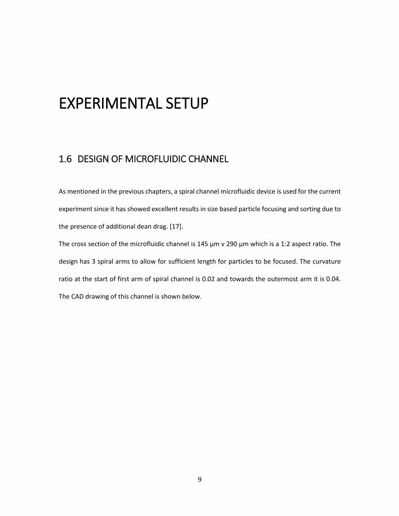
1.6 DESIGN OF MICROFLUIDIC CHANNEL

As mentioned in the previous chapters, a spiral channel microfluidic device is used for the current

experiment since it has showed excellent results in size based particle focusing and sorting due to

the presence of additional dean drag. [17].

The cross section of the microfluidic channel is 145 μm v 290 μm which is a 1:2 aspect ratio. The

design has 3 spiral arms to allow for sufficient length for particles to be focused. The curvature

ratio at the start of first arm of spiral channel is 0.02 and towards the outermost arm it is 0.04.

The CAD drawing of this channel is shown below.

10

Figure 2.1 Design of Spiral Microfluidic Channel

1.7 FABRICATION OF MOLD AND PDMS DEVICE

Soft lithography is used to fabricate microfluidic device. A mold with the reverse features of spiral

microfluidic channel is fabricated by coating a negative photoresist on a silicon wafer.

Two spin coats of SU-8 2150 (Microchem Corp.) are used to achieve a coating of height 145 μm

on a 4 inch diameter silicon wafer. This is followed by UV exposure using a Printed mask (from

CAD/Art Services, Inc.), Post exposure bake and development. The details of the baking

temperature, time and spin coating speed is are mentioned in Appendix A.

Once the mold is ready Polydimethylsiloxane (PDMS) is poured, degassed and cured to obtain

multiple copies of devices. A Sylgard® 184 silicone elastomer kit (Dow Corning Corp.) is used. The

PDMS copy is bonded to glass slide using plasma treatment to obtain the microfluidic device.

11

Photograph of this spiral channel microfluidic device fabricated using soft-lithography process is

shown below.

Figure 2.2 Fabricated Spiral Channel Microfluidic device

1.8 PREPARATION OF PARTICLE SOLUTION

Neutrally buoyant (density of 1 gm/ml) rigid polystyrene particles (Cospheric LLC) of diameter 24

μm are used for the experiment. These particles are mixed in a 0.1% Tween80 solution of Distilled

water to avoid cluster formation. The particles are mixed at a very low concentration of 0.03%

w/w to avoid inter particle interactions when they are flowing through the microfluidic channel.

The resulting confinement ratio (particle diameter/channel’s hydraulic diameter) is 0.12.

12

1.9 MICROSCOPE SETUP

A Nikon microscope mounted with a Photron FastCam SA4 high speed camera capable of

recording 512 x 512 pixel images at 13,500 FPS is used. To view the live feed from camera, to

record images and to control the settings of the high speed camera; a PC is connected to camera

with Photron Fastcam viewer software installed. A Sola Light engine (Lumencor Inc.) is joined with

the microscope for light source.

The camera and microscope are fixed to the breadboard on table. A 3-Axis MicroBlock compact

flexure stage with differential micrometers (Thorlabs Inc.) for precise movement in 1 μm steps is

used as a z-stage for vertical movement of microfluidic device. Objective lenses of magnification

50x is used for experimentation. This setup is shown in the figure below.

Figure 2.3 Microscope Setup

13

1.10 EXPERIMENTAL PROCEDURE

The microfluidic device is cleaned using a 3M tape to remove any smudges before mounting it on

the z-stage. The inlet is attached to a 10 ml BD syringe via a luer attachment, tubes and elbows.

The syringe is filled with 0.03% solution of 24 μm diameter particles in Distilled water. The outlet

is connected via an elbow joint to a tube which collects the solution in a test tube. Harvard

apparatus syringe pump (11 plus) is used to pump the solution into the microfluidic device at

required flow rate. These connections are shown below.

Figure 2.4 Device Mounted on z-stage

14

DATA COLLECTION AND DATA ANALYSIS

1.11 INTRODUCTION

The previous chapter discussed the experimental setup which is used to determine the slip

velocity of laterally focused particles. The current chapter discusses the exact step by step

experimental procedure.

Section 3.2 discusses the principle of microscope focusing which can be used to measure the

height of an object. Since the light beam emitted from the microscope has to travel through 3

different media before it is incident on the particle. Travel of focal plane of the microscope does

not have a 1:1 relationship with the travel of the z-stage. This relationship is discussed in section

3.3.

Procedure for identification of particle locations in vertical plane is discussed in section 3.4.

Section 3.5 discusses image processing done to obtain a focus measure and verify the visual

results of particle location in vertical plane.

Once the particle’s location in the vertical plane is known, image acquisition at sufficiently high

frame rates is carried out with the lens focal plane coincident with the plane of freely flowing

particles. A MatLab script for Circle edge detection is written, which traces the particles across

the successive frames of the acquired images. The same edge detection tool is used for measuring

the particles location in the horizontal plane away from the channel inner wall. This entire process

of obtaining the horizontal position and velocity of particles is discussed in section 3.6.

15

Section 3.7 discusses the error introduced in the results of particle velocity calculation.

Section 3.8 deals with the computation of undisturbed fluid velocity in the channel.

Computational Fluid Flow analysis through spiral channel in the absence of particles is carried out

using COMSOL MultiPhysics. Once the undisturbed velocity is computed, slip velocity can be easily

obtained.

1.12 MEASUREMENT OF OBJECT’S HEIGHT USING MICROSCOPE

To understand how microscopes could be utilized to measure the height of the channel, it’s

important to know how an objective lens works.

Figure 3.1 Measuring Height of Objects using a Microscope

The “Working distance” of objective lens remains constant for a given medium and is generally

provided by the Lens manufacturer along with additional data such as its Numerical Aperture. At

position A (Figure 3.1), the focal plane of the lens is coincident with the bottom surface of the

16

object. To get the top surface of Object in focus, the focal plane has to be moved by exactly the

same amount as the height of the Object. This can either be done by keeping the object on a fixed

stage and traversing the microscope in the upward direction (as shown in the schematic) or by

keeping the microscope fixed and placing the object on a z-stage which enables vertical

movement.

The accuracy of this method depends on the “Depth of focus” of the objective lens. Many

Objective lenses have a sufficiently large depth of focus as a result of which the object seems to

be in focus for a long range of vertical movement of focal plane. For the current study the height

of spiral micro-channel is 145 µm and particles have a diameter of 24 µm. This requires the depth

of focus to be in the range of few microns if height of particle is to be precisely measured.

The lens used in the current study is a 50x magnification lens with a depth of focus of 0.9 µm. The

microscope is kept fixed while a highly precise Z-stage with a least count of 1 µm in the vertical

direction is utilized which enables height measurements as small as 1 µm. Details of Lens, z-stage

and Microscope are discussed in Chapter 2.

1.13 RELATIONSHIP BETWEEN Z-STAGE MOVEMENT AND THE FOCAL

PLANE MOVEMENT

From section 3.2 it seems that there is a 1:1 relationship between movement of z-stage and the

lens’s focal plane. But that is only true if the working distance of the lens is constant. If the medium

between the object of interest and the lens keeps on the changing the relationship is no more

equal. For our case of determining height of particles flowing in a spiral microscopic channel the

17

light beam which is incident on the microscopic spherical particle surface has to travel through

three different mediums of Air, PDMS and Water. This is shown schematically below.

Figure 3.2 Schematic cross sectional view of particle being focused under microscope

From Snell’s Law, when light passes through a medium, the direction of propagation subtends an

angle with normal by a relation

𝑛𝑛1𝑛𝑛2

= ∝2∝1

Equation 3.1

Where,

𝑛𝑛1 𝑎𝑎𝑛𝑛𝑑𝑑 𝑛𝑛2 = refractive index of medium 1 and 2 respectively

∝1 𝑎𝑎𝑛𝑛𝑑𝑑 ∝2 = Angle subtended by the light rays

Angle subtended by the objective lens in the air is calculated from the lens manufacturer’s

specifications. Snell’s law gives the subtended angle as it passes through PDMS and Water

respectively.

Change in subtended angle changes the working distance of the lens too. Further, the working

distance changes constantly depending on the length through which the light rays have to travel

through a medium. It is depicted through a ray diagram below. From this diagram it is seen that

18

as we move from case1 to case2, a 50 unit movement of focal plane requires 33.7113 unit of

movement for z-stage.

Figure 3.3 Ray Diagram depicting that movement of Z-stage and Focal Plane are not equal

This shows that in the presence of two or more mediums, if the stage is moved vertically by a

certain amount, the focal plane does not move vertically by equal amount.

For the microfluidic device used in the experiments, channel cross section height is 145 μm and

thickness of PDMS slab is 1905 μm. The refractive index of air and water are available from

standard property charts whereas the refractive index of PDMS is obtained from the product data

sheet of manufacturer (Dow Corning).

Sr. No. Medium Refractive index Angle subtended by objective lens

1 Air 1 36.86°

2 PDMS 1.4 25.377°

3 Water 1.33 26.816°

Table 3.1 Refractive index of different media

19

Using these values, an equation for the relationship between movement of z-stage and movement

of focal plane is derived. Its derivation is carried out in Appendix B. The relationship obtained is:

𝑀𝑀𝑀𝑀𝑀𝑀𝐷𝐷𝑀𝑀𝐷𝐷𝑛𝑛𝑀𝑀 𝑀𝑀𝑜𝑜 𝐹𝐹𝑀𝑀𝐹𝐹𝑎𝑎𝐹𝐹 𝑃𝑃𝐹𝐹𝑎𝑎𝑛𝑛𝐷𝐷 = 1.48 × 𝑀𝑀𝑀𝑀𝑀𝑀𝐷𝐷𝑀𝑀𝐷𝐷𝑛𝑛𝑀𝑀 𝑀𝑀𝑜𝑜 𝑧𝑧 𝑠𝑠𝑀𝑀𝑎𝑎𝑠𝑠𝐷𝐷 Equation 3.2

The above equation has been derived theoretically but it needs to be verified practically too since

all the future readings and calculations depend on the authenticity of the above equation. For

this, a two-step microfluidic device is fabricated for the sole purpose of verifying the above

equation. Its schematic is shown below:

Figure 3.4 schematic cross sectional view of a two-step microfluidic device

The focal plane is traversed between three elevations: a, b and c indicated in the schematic (Figure

3.4) above. Detection of these elevations is made possible by marking the PDMS surface at these

elevations with a black marker pen (Marks visible in Figure 3.5).

This two-step microfluidic device is kept on the z-stage and moved vertically such that the markers

at elevations c, b and a are focused one by one respectively. The movement of z-stage is measured

and compared with the actual distance between the three elevations. It is experimentally verified

20

that the error in travel of focal plane is within 0.56% of the theoretical calculations for the two

step device. The picture of actual two-step microfluidic device is shown below.

Figure 3.5 Photograph of the two step microfluidic device

The experimental verification of the relationship between z-stage movement and focal plane

movement creates confidence in using Equation 3.2 which is derived for spiral microfluidic

channel.

1.14 IDENTIFICATION OF FOCUSING POSITIONS IN VERTICAL PLANE

The spiral microchannel used has a height of 145 μm. The bottom of the channel is identified and

the z-stage reading at that elevation is treated as a datum from which height of the particles could

be measured.

To identify the channel bottom an identifying mark has to be made on the glass slide on which

the PDMS is bonded. Use of marker pens does not work well for two reasons. The plasma

21

oxidation of the glass surface is affected and creates bonding issues with PDMS if an oil based

marker is used. An alcohol based marker gets rubbed away when fluid flows through the channel

making the device unusable for channel’s bottom measurement.

To circumvent this issue, a microscopic scratch is created on the Glass Slide before bonding PDMS

with it. The scratch is very minute and does not leak the device when operational but the scratch

is still clearly noticeable when focused under the microscope’s 50x lens (Figure 3.6). The scratch

is created at a location such that it is exposed to the water flowing through the channel. If the

scratch gets in contact instead with PDMS after bonding, the particle height determination won’t

be accurate since the water medium is not present during channel datum measurement. Image

of the scratch visible under microscope is shown below.

Figure 3.6 Scratch made for channel bottom measurement

For convenience, the procedure of identifying particles height is discussed for the following

experimental conditions in this entire section for ease of explanation, though the same procedure

was followed for other flow rate and particle size too.

Flow rate: 160 μL/min

Particle size: 24 μm

22

To identify the particle’s laterally focused position in the vertical plane, the images have to be

acquired when the particles are flowing through the spiral channel in an inertial flow. The entire

setup is kept stationary for the next few hours (except for the precise vertical movement of z-

stage) of data acquisition as the slightest vibrations may affect the accuracy of readings.

The image acquisition starts with the channel’s bottom coincident with the focal plane by focusing

on to the scratch by rotating the dial of z-stage. Two such images when the channel bottom was

focused are shown below.

Figure 3.7 Left: Scratch in focus, Right: Two particles in single frame with one in focus while other is not

It is clearly visible that the scratch is completely focused on the image. The image on the right

shows the channel bottom in focus where the scratch is focused but the particle which is flowing

freely inside the channel is not in focus since it is above the channel’s bottom surface.

Now once the datum is established, the z-stage is moved in steps of 5 μm till the total travel of z-

stage is 95 μm. This corresponds to a travel of 140.6 μm for the movement of focal plane (from

Equation 3.2) starting exactly from the channel bottom surface to just 4.6 μm below the channel

top surface. This ensures that location of particles could be identified throughout the vertical

plane of channel.

23

Image acquisition is done at 10,000 FPS for about 1.4 seconds for all the 5 um steps of z-stage

movement. The acquired images are initially manually scanned to identify the most focused

images of particles. It was observed that the particles were highly crisp and sharp when the z-

stage was moved 15 μm and 45 μm w.r.t. the datum (channel bottom surface). This corresponds

to the actual height of 22.2 μm and 66.7 μm above the datum.

Sample images acquired at each elevation (in steps of 5 μm of z-stage) starting from channel

datum are shown below.

26

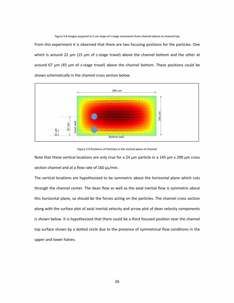
Figure 3.8 Images acquired in 5 um steps of z-stage movement from channel datum to channel top

From this experiment it is observed that there are two focusing positions for the particles. One

which is around 22 μm (15 μm of z-stage travel) above the channel bottom and the other at

around 67 μm (45 μm of z-stage travel) above the channel bottom. These positions could be

shown schematically in the channel cross section below.

Figure 3.9 Positions of Particles in the vertical plane of channel

Note that these vertical locations are only true for a 24 μm particle in a 145 μm x 290 μm cross

section channel and at a flow rate of 160 μL/min.

The vertical locations are hypothesized to be symmetric about the horizontal plane which cuts

through the channel center. The dean flow as well as the axial inertial flow is symmetric about

this horizontal plane, so should be the forces acting on the particles. The channel cross section

along with the surface plot of axial inertial velocity and arrow plot of dean velocity components

is shown below. It is hypothesized that there could be a third focused position near the channel

top surface shown by a dotted circle due to the presence of symmetrical flow conditions in the

upper and lower halves.

27

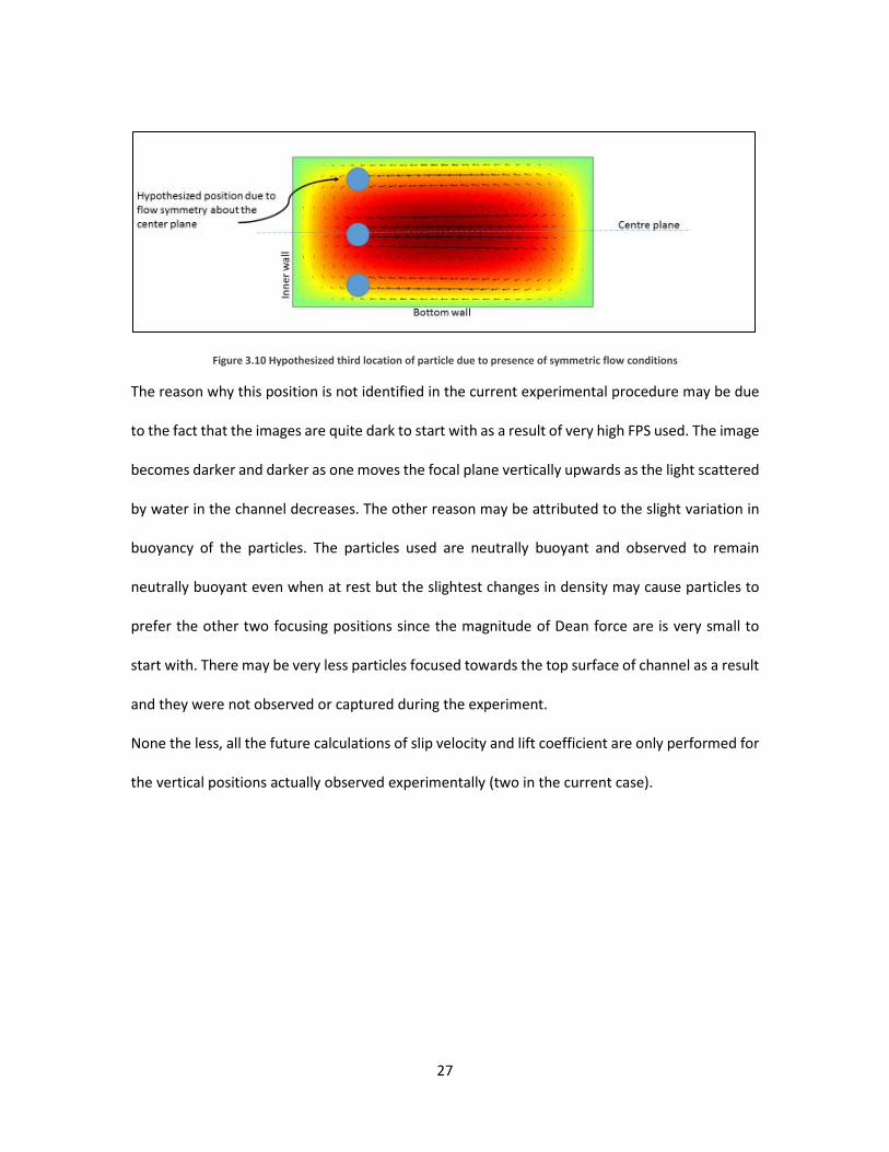
Figure 3.10 Hypothesized third location of particle due to presence of symmetric flow conditions

The reason why this position is not identified in the current experimental procedure may be due

to the fact that the images are quite dark to start with as a result of very high FPS used. The image

becomes darker and darker as one moves the focal plane vertically upwards as the light scattered

by water in the channel decreases. The other reason may be attributed to the slight variation in

buoyancy of the particles. The particles used are neutrally buoyant and observed to remain

neutrally buoyant even when at rest but the slightest changes in density may cause particles to

prefer the other two focusing positions since the magnitude of Dean force are is very small to

start with. There may be very less particles focused towards the top surface of channel as a result

and they were not observed or captured during the experiment.

None the less, all the future calculations of slip velocity and lift coefficient are only performed for

the vertical positions actually observed experimentally (two in the current case).

28

1.15 USE OF FOCUS MEASURE TO VERIFY THE PARTICLES POSITION IN

VERTICAL PLANE

To make sure that no human error or human preference plays role in determining which particle

looks the sharpest and most focused while determining the height of the particles, a MatLab script

was written which measures the sharpness of image and assigns a value to it. This value is termed

Global Variance Focal Measure or GVFM in short for all the future references. The higher the

GVFM value the sharper is the image.

To understand how this MatLab script works it is necessary to understand the way image files are

stored. The grey scale image captured by the microscope is actually values of pixel stored as rows

and columns of a matrix. The value of each element of the matrix is the brightness of the image.

A perfect white is assigned a value of 255, perfect black a value of 0 and all the values in between

for the 244 shades of grey. There are many ways to identify the focus measure of an image. The

sharpest image has the most contrasting edge. As a result, the gradients as we move across the

pixel values is the steepest for the most focused image. The other way is to calculate the variance

of pixel values. The most contrasting image has a high value of variance. Global variance of the

image is performed for the current study to obtain its focal measure.

The images captured at each elevation of the z-stage were of size 512 x 768 pixels. A moving

window of size 15 x 15 pixels is created which moves across the entire image and calculates local

variance for each pixel as it moves around. The variance of these local variances is called the

Global Variance Focal Measure (GVFM). MatLab code used for calculating GVFM is attached in

Appendix C.

29

To show that the above script works, a few sample images are taken where the image is initially

not clear, gradually as the focal plane is traversed in vertical direction the image is completely

focused and later the image again becomes fuzzy when the focal plane crosses the object’s

position. The graph of GVFM values vs the movement of focal plane is shown below (Figure 3.11).

The maxima of the graph is the most focused image.

Figure 3.11 GVFM value of a image vs Movement of Focal Plane in vertical direction

To obtain the most accurate measure of the degree of focus of particles a statistical histogram of

GVFM values for all the images acquired for a given z-stage height is obtained. A sample GVFM

histogram of all the images (containing particles) acquired at a z-stage height of 20 μm from

datum is shown below.

30

Plot 3.1 GVFM histogram at 20 um z-stage height

It is observed that there are two peaks for the GVFM values. This is in consistency with the visual

findings of two focusing positions in the vertical plane. The peak around 750,000 GVFM shows

that there are many particles focused at a vertical height near to the focal plane. Again there is a

peak at around 260,000 GVFM indicating there are many particles clustered together at a vertical

height but not so well focused.

Only the highest peak of around 750,000 GVFM is of importance as it indicates the measure of

nearest particles from the focal plane. This peak GVFM value is obtained for all the z-stage

elevations (in 5 µm steps) and are plotted as a function of z-stage movement. The peaks of the

curve should show the vertically focused positions of the images.

0123456789

10

GVFM Histogram at 20 um z-stage height

31

Plot 3.2 GVFM of particles vs z-stage movement

Clearly, in plot 3.2 the two peaks observed are at 15 μm and 45 μm heights confirming the similar

visual deductions for the heights of particles.

Additionally, the maxima of GVFM plot is also used to identify the channel datum surface within

an accuracy of 1 μm. A plot of GVFM vs z-stage travel for 10 μm is shown below (Plot 3.3).

0

200000

400000

600000

800000

1000000

1200000

1400000

1600000

0 5 10 15 20 25 30 35 40 45 50 55 60 65 70 75 80 85 90 95

GVFM

Movement of z-stage from the channel bottom surface

GVFM of particles vs z-stage movement

GVFM valueof particles

Base GVFMof imageswithoutparticle

32

Plot 3.3 GVFM value vs z-stage movement for channel bottom detection

1.16 CALCULATION OF PARTICLE VELOCITY

Since the particle’s height in the vertical plane is now known accurately, the z-stage is set such

that the particle elevation is coincident with the focal plane. Image acquisition is done at 10,000

FPS for about 1.4 seconds. Images for particles moving across the width are carefully selected. A

sample particle moving across the width of the acquired image in successive frames is shown

below (Figure 3.12).

33

Figure 3.12 Particle moving across successive frames of acquired images

About 20 such highly focused particles (using GVFM height verification) are selected. Each particle

consists of around 15 to 20 frames (Only 8 frames of one such particle are shown above)

To calculate the velocity of this particle it is necessary to trace the pixel information for the center

of this particle as it moves across the width of the image in the successive frame. The particle

which is visible as a black circle in the images is detected using edge detection tool available in

MATLAB functionality. Adjusting the contrast of the image, defining sensitivity of the roundness

of the circle to be detected and pixel radius range of the circle to be detected, pixel location of

the circle and the radius of circle in terms of pixels could be identified. The script is attached in

Appendix D. The circle detection in action is shown below.

Figure 3.13 Circle detection for velocity measurement in action, image snapshots

34

Once the circle pixel locations are identified it is straightforward to obtain the velocity of particle

in terms of pixels per second. The width of the microfluidic channel which is visible in the images

is of known dimension (290 μm) and is used as a standard to obtain the speed of particles in

meters per second.

About 15 to 20 frames are acquired as the particle moves from left of image to right. The time

interval between two successive frames is 1/10,000 seconds. It takes approximately 3

milliseconds for the particle as it moves across the image width.

The circle detection may have an error of couple of pixels while the particle moves by around 8-

10 pixels between two frames. This may introduce an error of about 10% in the velocity

measurement. Hence, circle detection and velocity measurement is done for every third frame

which reduces the error greatly to about a couple of pixels for the particle movement of about 30

pixels (3% error).

For each particle about 4 to 5 values of velocity are obtained as it moves across the image width.

Now, since the pixel information of circle’s center is available and the channel’s vertical walls are

visible in the images, the horizontal distance of that particle from the channel vertical walls could

be obtained. This would help identify the focused position of the particle in the horizontal plane.

The Matlab script for distance measurement of particle’s center from channel’s inner wall is in

appendix D.

Now, as mentioned earlier a 24 μm particle inside a flow of 160 μL/min has two focusing positions

in the vertical plane. One is 22 μm above the channel bottom and other 67 is μm above the

bottom. For the 22 μm above the bottom position, particles are traced and their velocities plotted

as a function of the horizontal distance of the particles from the inner wall. 3 to 5 velocity values

are obtained for each particle and the about 15-20 such particles are measured. Each particle is

35

color coded and the colored vertical line indicates the range of velocities which were measured

for that particle.

Plot 3.4 Particle velocity vs particle distance from inner wall

1.17 SPREAD OF PARTICLES INSIDE THE CHANNEL AND ESTIMATION

OF ERROR

It has to be observed that the focused particles have a narrow range of spread in the vertical plane

as compared to the horizontal plane. While measuring the vertical focused positions, the GVFM

drops sharply just 5 μm above or below the maxima values as evident from plot 3.2. This suggests

that the particles are highly focused in the vertical plane within a narrow range of ±5 μm. And the

few particles which may have a wider spread are not considered for the next stage of data analysis

at all. The 15 to 20 particles which are selected for velocity calculations have the GVFM values of

the peaks of plot 3.2.

0.06

0.07

0.08

0.09

0.1

0.11

0.12

65 75 85 95 105 115 125

part

icle

vel

ocity

(m/s

)

Distance from inner wall (um)

Particle Velocity vs particle distance from inner wall

36

On the other hand particles have a comparatively wider spread in the horizontal plane. Particles

are observed at a distance of about 60 μm from inner wall to about 130 μm from inner wall. This

is a spread of 110 μm or 4.6 times the particle diameter. This spread is not sufficiently small like

the one in vertical plane and hence the particle velocity plots, calculation of slip velocity and

calculation of lift coefficients is done as a function of particle’s distance from inner wall.

The reason why particles are highly focused in the vertical plane compared to the horizontal plane

could be attributed to the cross sectional area of the channel and the resulting Inertial Velocity

flow profile. The shear gradients in the vertical plane are steeper than the ones in horizontal plane

due to the 1:2 aspect ratio.

The location of the particle under consideration is obtained accurately in the horizontal plane.

The only error accrued is the error in circle center detection which is not more than a couple of

pixels. But determination of location in vertical plane is done in steps of 5 μm which results in an

error or ±5 μm in the vertical position determination.

To make sure that the slip velocity of particle is accurately determined it should be kept in

consideration that the particle may be 5 μm above or below the selected location and hence the

undisturbed fluid flow velocity has to be obtained 5 μm above and below the particle.

1.18 UNDISTURBED FLUID FLOW VELOCITY

The velocity of particle is now determined experimentally but the velocity of undisturbed fluid

flow should also be known to calculate the slip velocity. The fluid velocity is calculated

computationally using COMSOL Multiphysics. Since the flow condition is laminar inside the spiral

microfluidic channel with low Reynolds number in the range of 10 to 20, the Flow conditions can

37

be accurately reproduced computationally within errors which are insignificant for the current

study.

A 3D curved one arm channel geometry is created with the curvature ratio equal to that of outer

arm of spiral microchannel device where experimental measurements are made. A single arm is

used so that computational resources could be better utilized in making the mesh size as small as

possible instead of solving for the entire three arms of the spiral geometry with a larger mesh size.

The geometry is shown below.

Figure 3.14 Spiral arm channel geometry created in Comsol interface

The grid size is between 5-10 μm in size across the channel cross section so that the dean vortices

generated could be accurately reproduced. The grid elements are elongated in the axial direction

and their lengths range from 20-30 μm since sufficient length of the curved arm is available for

the flow to fully develop.

The flow is assumed to be laminar and stationary. The resulting conservation of mass and

momentum equations are as below:

38

𝛻𝛻 ∙ (𝒖𝒖) = 0 Equation 3.3

𝒖𝒖 ∙ 𝛻𝛻𝒖𝒖 = −1𝜌𝜌𝛻𝛻𝛻𝛻 + 𝜈𝜈𝛻𝛻2𝒖𝒖 Equation 3.4

The boundary conditions are mentioned below:

At inlet,

𝒖𝒖 = −𝑈𝑈0𝒏𝒏 Equation 3.5

Where U0 is the average velocity obtained by dividing the flow rate by cross sectional area.

At Outlet,

[−𝛻𝛻 + 𝜋𝜋(∇𝒖𝒖 + (∇𝒖𝒖)𝑇𝑇)]𝒏𝒏 = −𝛻𝛻𝑜𝑜𝒏𝒏 Equation 3.6

Where p0 is the outlet pressure which is atmospheric.

At channel walls no slip boundary condition is used.

𝒖𝒖 = 0 Equation 3.7

The initial conditions are

𝒖𝒖 = 0 Equation 3.8

𝛻𝛻 = 0 Equation 3.9

The cross section (145 μm x 290 μm) of the channel arm at which the velocity components are

measured is chosen sufficiently far away (about 7,500 μm) from the inlet so that the flow is fully

developed but at the same time the selected cross section is a little bit before the outlet (about

2,000 μm) so that the velocity profile and Dean vortices do not get disturbed due to the presence

of outlet boundary condition.

In plot 3.5, velocity of particles which are focused in a plane 22 μm above channel bottom were

plotted. On the same plot, the undisturbed axial component of fluid flow profile is plotted. As

discussed in section 3.7, the particle may be vertically in the ±5 µm range from the measured 22

39

µm height and the undisturbed fluid velocity obviously varies across this 10 µm variation in height.

These Limits of fluid velocity are plotted as red and green lines below.

Plot 3.5 Range of particle velocity and undisturbed fluid velocity

For the above case of Reynolds number 13.7, particle diameter 24 μm and vertical focused

position of 22 μm from channel bottom, it is observed that the particle velocity spread for each

particle (shown by a vertical blue line) is quite small and it could be replace for a single value of

particle’s average velocity. Such graph is plotted below (Plot 3.6).

0.04

0.05

0.06

0.07

0.08

0.09

0.1

0.11

0.12

65 75 85 95 105 115 125

part

icle

vel

ocity

(m/s

)


fluid velocity17 um abovechannelbottom


40

Plot 3.6 Average particle velocity and Fluid velocity

Subtraction of Undisturbed fluid flow velocity from the average particle velocity gives the slip

velocity of particle.

𝑀𝑀𝑠𝑠𝑠𝑠𝐿𝐿𝑠𝑠 = 𝑀𝑀𝑠𝑠𝑑𝑑𝑝𝑝𝐿𝐿𝑝𝑝𝐿𝐿𝑠𝑠𝑑𝑑 − 𝑀𝑀𝑆𝑆𝑠𝑠𝑓𝑓𝐿𝐿𝑑𝑑 Equation 3.10

Plot 3.7 Slip velocity

0.040000

0.050000

0.060000

0.070000

0.080000

0.090000

0.100000

0.110000

0.120000

65 75 85 95 105 115 125

Part

icle

vel

ocity

(m/s

)

particles distance from inner wall (um)

Average velocity ofparticle

Fluid velocity 17 umfrom bottom

fluid velocity 27 umfrom bottom

0.0000

0.0100

0.0200

0.0300

0.0400

0.0500

0.0600

60 70 80 90 100 110 120 130

Slip

vel

ocity

(m/s

)


41

The red and green data points are the upper and lower limits of the slip velocities while the blue

points indicate the average slip velocity. Upper and Lower limits are obtained by subtracting the

±5 µm range of fluid flow velocity from the average velocity of particles.

42

RESULTS AND DISCUSSION: SLIP VELOCITY AND LIFT COEFFICIENT

1.19 SLIP VELOCITY OF 24 µM PARTICLES AT RE = 13.7 AND 17.2

With the procedure discussed in Chapter 3 the slip velocity for 24 µm particles at two different

Reynolds number is calculated in this Chapter. The Reynolds number used are 13.7 and 17.2

corresponding to the flow rates of 160 µL/min and 200 µL/min respectively. The particles are

visually focused at both these conditions.

The first step is the determination of particle positions in vertical plane. The number of focusing

positions and their elevations are tabulated below.

Sr. No.

Reynolds Number

Flow rate (µL/min)

Locations of vertical focusing position from channel bottom

(µm)

1 13.7 160 22 67

2 17.2 200 15 67

Table 4.1 Vertical focusing positions of 24 um particles

The particle velocities are obtained next as a function of Distance from inner wall. For a flow rate

of 160 µL/min the particle velocities at two different elevations of 22 µm and 67 µm are plotted

below.

43

Plot 4.1Particle velocity plot, Re=13.7, Vertical focus position of 22 um

Plot 4.2 Particle velocity plot, Re=13.7, Vertical focus position of 67 um

0.04

0.05

0.06

0.07

0.08

0.09

0.1

0.11

0.12

60 70 80 90 100 110 120 130

Velo

city

(m/s

)


0.04

0.05

0.06

0.07

0.08

0.09

0.1

0.11

0.12

60 70 80 90 100 110 120 130

Velo

city

(m/s

)


44

The corresponding fluid velocity profiles at 22 µm and 67 µm height above the channel bottom

are now impressed on the previous plots of particle velocity.

Plot 4.3 Range of particle velocity, Re=13.7, Vertical focus position of 22 um


0.04

0.05

0.06

0.07

0.08

0.09

0.1

0.11

0.12

0.13

0.14

60 70 80 90 100 110 120 130

Velo

city

(m/s

)




0.04

0.05

0.06

0.07

0.08

0.09

0.1

0.11

0.12

0.13

0.14

60 70 80 90 100 110 120 130

Velo

city

(m/s

)


fluidvelocity 62um abovechannelbottom


45

Calculating the average velocity of each particle and the corresponding slip velocity:

Plot 4.5 Slip velocity of particle 22 um above channel bottom, Re=13.7


0.0000

0.0100

0.0200

0.0300

0.0400

0.0500

0.0600

60 70 80 90 100 110 120 130

Slip

vel

ocity

(m/s

)


average slipvelocity

upper limit:slipvelocity

lower limit: slipvelocity

-0.025000

-0.020000

-0.015000

-0.010000

-0.005000

0.00000060 70 80 90 100 110 120 130

Slip

Vel

ocity

(m/s

)



upper limit: slipvelocity

lower limit: slipvelocity

46

The same procedure is repeated at Re=17.2 corresponding to a flow rate of 200 µL/min. The

particle velocities at two vertical elevations of 15 µm and 67 µm from channel bottom are plotted

below.

Plot 4.7 Particle velocity, Re= 17.2, Vertical focus position of 15 um

Plot 4.8 particle velocity, Re=17.2, Vertical focus position of 67 um

0.04

0.06

0.08

0.1

0.12

0.14

0.16

60 70 80 90 100 110 120 130

Velo

city

(m/s

)


0.04

0.06

0.08

0.1

0.12

0.14

0.16

60 70 80 90 100 110 120 130

Velo

city

(m/s

)


47

The corresponding fluid velocity profiles 15(+5 and -3) µm and 67±5 µm above the channel bottom

are now impressed on the previous plots of particle velocity.


Plot 4.10 Range of particle velocity, Re=17.2, vertical focus position of 67 um

0.02

0.04

0.06

0.08

0.1

0.12

0.14

0.16

60 70 80 90 100 110 120 130

Velo

city

(m/s

)




0.08

0.09

0.1

0.11

0.12

0.13

0.14

0.15

0.16

60 70 80 90 100 110 120 130

Velo

city

(m/s

)


fluid velocity62 umabovechannelbottom

fluid velocity72 umabovechannelbottom

48

Calculating the average velocity of each particle and the corresponding slip velocity:



0.000000

0.020000

0.040000

0.060000

0.080000

0.100000

0.120000

60 70 80 90 100 110 120 130

Slip

vel

ocity

(m/s

)



upper limit: slipvelocity

lowe limit: slipvelocity

-0.030000

-0.025000

-0.020000

-0.015000

-0.010000

-0.005000

0.00000060 70 80 90 100 110 120 130

Slip

vel

ocity

(m/s

)



lower limit:slip velocity

upper limit:slip velocity

49

1.20 LIFT COEFFICIENTS OF 24 µM PARTICLES AT RE=13.7 AND 17.2

As already mentioned in section 1.4, most of the theoretical work done in the past few decades

suggest a linear relationship between Lift Force and particle’s slip velocity.

Hence, the inertial lift could be expressed in the form of

𝐹𝐹𝑠𝑠𝐿𝐿𝑆𝑆𝐿𝐿 = 𝐶𝐶𝑠𝑠 × 𝑀𝑀𝑠𝑠𝑠𝑠𝐿𝐿𝑠𝑠 Equation 4.1

Where,

𝐹𝐹𝑠𝑠𝐿𝐿𝑆𝑆𝐿𝐿= Lift force on the particle

𝑀𝑀𝑠𝑠𝑠𝑠𝐿𝐿𝑠𝑠= Slip velocity of the particle

𝐶𝐶𝑠𝑠= Lift coefficient

At this moment, the form, expression or dependence of 𝐶𝐶𝑠𝑠 is not known. But its numerical value

could be obtained from equation 4.1 if the Lift force and slip velocity of particle is known. The slip

velocity is already calculated in the preceding section.

A particle which flows through a spiral channel with inertial flow achieves lateral equilibrium due

to the presence of two forces. The first force is the Lift force due to the presence of shear gradient

and wall effect. The other force is the Dean drag due to the presence of secondary Dean flow in

the spiral channel. These two forces must balance each other for lateral equilibrium of particles

to be achieved.

𝐹𝐹𝑠𝑠𝐿𝐿𝑆𝑆𝐿𝐿 + 𝐹𝐹𝑑𝑑𝑑𝑑𝑑𝑑𝑑𝑑 = 0 Equation 4.2

Dean flow is a highly viscous and a non-inertial secondary flow with vanishingly small Reynolds

number and as a result the Stokes’ flow assumption is valid. The Dean drag could be obtained

from the Stokes Drag equation given by:

50

𝐹𝐹𝑑𝑑𝑑𝑑𝑑𝑑𝑑𝑑 = 6𝜋𝜋𝜋𝜋𝑅𝑅𝜋𝜋 Equation 4.3

Where,

µ = dynamics viscosity of water

R = radius of particle

𝜋𝜋= Dean flow velocity relative to the particle

The Dean Flow velocity components are obtained from the computational study of fluid flow

through the curved arm of the spiral channel. Once the velocity components are known 𝐹𝐹𝑑𝑑𝑑𝑑𝑑𝑑𝑑𝑑 is

calculated from equation 4.3 and 𝐹𝐹𝑠𝑠𝐿𝐿𝑆𝑆𝐿𝐿 from equation 4.2

For a given particle, its location is determined, slip velocity obtained, Dean Drag calculated at that

location and value of Lift coefficient is obtained.

Since the slip velocities were obtained as a function of distance from inner wall, a similar format

is followed for the calculation of Lift coefficient too.

The calculations and the resulting Lift coefficients for Re=13.7 and vertical focus position of 22 µm

from channel bottom are shown in the tabular format below.

51

Lift Coefficient for Vertical focus position of 22 µm, Re=13.7 Pa

rtic

le

no.

Dist

ance

fr

om

inne

r Dean velocity (m/s) Slip Velocity

(m/s)

Lift force (N) Lift coefficient

VY VZ FLift(Y) FLift(Z) CL(Y) CL(Z) 1 85.6785 -0.0001417172 0.0000215520 0.0421648623 3.2039E-11 -4.8725E-12 7.5986E-10 -1.1556E-10

2 74.333 -0.0001260000 0.0000263000 0.0418796270 2.8486E-11 -5.9459E-12 6.8019E-10 -1.4198E-10

3 98.5057 -0.0001560000 0.0000163000 0.0415656460 3.5268E-11 -3.6851E-12 8.4850E-10 -8.8657E-11

4 118.5473 -0.0001698147 0.0000086017 0.0411749199 3.8392E-11 -1.9447E-12 9.3241E-10 -4.7229E-11

5 85.9333 -0.0001420000 0.0000215000 0.0384149310 3.2103E-11 -4.8607E-12 8.3570E-10 -1.2653E-10

6 73.8946 -0.0001250000 0.0000265000 0.0432855340 2.8260E-11 -5.9911E-12 6.5287E-10 -1.3841E-10

7 84.0831 -0.0001400000 0.0000222000 0.0404723140 3.1651E-11 -5.0190E-12 7.8205E-10 -1.2401E-10

8 123.5458 -0.0001720000 0.0000068100 0.0386405090 3.8886E-11 -1.5396E-12 1.0063E-09 -3.9844E-11

9 91.7066 -0.0001490000 0.0000191000 0.0412216230 3.3686E-11 -4.3181E-12 8.1719E-10 -1.0475E-10

10 94.0511 -0.0001510000 0.0000181000 0.0446689250 3.4138E-11 -4.0920E-12 7.6425E-10 -9.1608E-11

11 91.8732 -0.0001490000 0.0000190000 0.0396205650 3.3686E-11 -4.2955E-12 8.5021E-10 -1.0842E-10

12 96.1425 -0.0001530000 0.0000173000 0.0411983440 3.4590E-11 -3.9112E-12 8.3960E-10 -9.4935E-11

13 68.4651 -0.0001170000 0.0000287000 0.0423384020 2.6451E-11 -6.4885E-12 6.2476E-10 -1.5325E-10

14 85.606 -0.0001420000 0.0000216000 0.0367733280 3.2103E-11 -4.8833E-12 8.7301E-10 -1.3280E-10

15 79.7529 -0.0001340000 0.0000240000 0.0423834130 3.0295E-11 -5.4259E-12 7.1478E-10 -1.2802E-10

Table 4.2 Lift coefficient for vertical focus position of 22 um, Re= 13.7

52

From the above table 4.2, components of Lift force are plotted below

Plot 4.13 Horizontal component of Lift force, Vertical position of 22 um, Re=13.7

Plot 4.14 Vertical component of Lift force, vertical position of 22 um, Re=13.7

0.0000E+00

5.0000E-12

1.0000E-11

1.5000E-11

2.0000E-11

2.5000E-11

3.0000E-11

3.5000E-11

4.0000E-11

4.5000E-11

60 70 80 90 100 110 120 130

Lift

For

ce F

lift(Y

) -(N

)


-7.0000E-12

-6.0000E-12

-5.0000E-12

-4.0000E-12

-3.0000E-12

-2.0000E-12

-1.0000E-12

0.0000E+0060 70 80 90 100 110 120 130

Lift

For

ce F

lift(

Z) -

(N)


53

From the same table 4.2, Lift coefficient components are plotted below:

Plot 4.15 Horizontal Lift coefficient, vertical position of 22 um, Re= 13.7

Plot 4.16 Vertical Lift coefficient, vertical position of 22 um, Re= 13.7

0.0000E+00

2.0000E-10

4.0000E-10

6.0000E-10

8.0000E-10

1.0000E-09

1.2000E-09

60 70 80 90 100 110 120 130

Lift

Coe

ffici

ent C

L(Y)


-1.8000E-10

-1.6000E-10

-1.4000E-10

-1.2000E-10

-1.0000E-10

-8.0000E-11

-6.0000E-11

-4.0000E-11

-2.0000E-11

0.0000E+0060 70 80 90 100 110 120 130

Lift

Coe

ffici

ent C

L(Z)


54

Similar procedure is followed for the same Re=13.7 but for the second vertical focus position of 67 µm from channel bottom to obtain Lift

coefficients.

Lift Coefficient for Vertical focus position of 67 µm, Re=13.7

Part

icle

no

.

Dist

ance

fr

om

inne

r w

all Dean velocity

(m/s) Dean velocity (m/s)


VY VZ FLift(Y) FLift(Z) CL(Y) CL(Z)

1 83.6111 0.0001905015 0.0000107533 -0.0088515870 -4.3069E-11 -2.4311E-12 4.8656E-09 2.7465E-10

2 94.3204 0.0002080000 0.0000086900 -0.0153850900 -4.7025E-11 -1.9646E-12 3.0565E-09 1.2770E-10

3 95.2556 0.0002090000 0.0000085000 -0.0159393580 -4.7251E-11 -1.9217E-12 2.9644E-09 1.2056E-10

4 88.8838 0.0002000000 0.0000097300 -0.0150867990 -4.5216E-11 -2.1998E-12 2.9971E-09 1.4581E-10

5 124.497 0.0002370000 0.0000031700 -0.0183109280 -5.3581E-11 -7.1667E-13 2.9262E-09 3.9139E-11

6 74.3841 0.0001730000 0.0000125000 -0.0094589300 -3.9112E-11 -2.8260E-12 4.1349E-09 2.9877E-10

7 74.7282 0.0001730000 0.0000124000 -0.0037822830 -3.9112E-11 -2.8034E-12 1.0341E-08 7.4119E-10

8 92.653 0.0002050000 0.0000090000 -0.0161902610 -4.6346E-11 -2.0347E-12 2.8626E-09 1.2568E-10

9 64.1457 0.0001500000 0.0000143000 -0.0074308150 -3.3912E-11 -3.2329E-12 4.5637E-09 4.3507E-10

10 72.3199 0.0001680000 0.0000129000 -0.0115784590 -3.7981E-11 -2.9164E-12 3.2804E-09 2.5188E-10

11 74.8012 0.0001740000 0.0000124000 -0.0096127340 -3.9338E-11 -2.8034E-12 4.0923E-09 2.9163E-10

12 85.7396 0.0001940000 0.0000103000 -0.0103028970 -4.3860E-11 -2.3286E-12 4.2570E-09 2.2602E-10

13 121.0269 0.0002350000 0.0000037700 -0.0199750380 -5.3129E-11 -8.5232E-13 2.6598E-09 4.2669E-11

Table 4.3 Lift Coefficient for vertical focus position of 67 um, Re=13.7

55

From the above table 4.3, components of Lift force are plotted below

Plot 4.17 Horizontal component of lift force, vertical position of 67 um, Re= 13.7

Plot 4.18 Vertical component of lift force, vertical position of 67 um, Re=13.7

-6.0000E-11

-5.0000E-11

-4.0000E-11

-3.0000E-11

-2.0000E-11

-1.0000E-11

0.0000E+0060 70 80 90 100 110 120 130

Lift

For

ce F

lift(Y

)-(

N)


-3.5000E-12

-3.0000E-12

-2.5000E-12

-2.0000E-12

-1.5000E-12

-1.0000E-12

-5.0000E-13

0.0000E+0060 70 80 90 100 110 120 130

Lift

For

ce F

lift(Z

)-(

N)


56

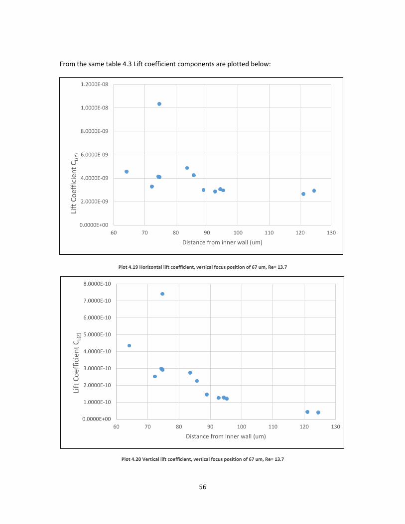
From the same table 4.3 Lift coefficient components are plotted below:

Plot 4.19 Horizontal lift coefficient, vertical focus position of 67 um, Re= 13.7

Plot 4.20 Vertical lift coefficient, vertical focus position of 67 um, Re= 13.7

0.0000E+00

2.0000E-09

4.0000E-09

6.0000E-09

8.0000E-09

1.0000E-08

1.2000E-08

60 70 80 90 100 110 120 130

Lift

Coe

ffici

ent C

L(Y)


0.0000E+00

1.0000E-10

2.0000E-10

3.0000E-10

4.0000E-10

5.0000E-10

6.0000E-10

7.0000E-10

8.0000E-10

60 70 80 90 100 110 120 130

Lift

Coe

ffici

ent C

L(Z)


57

Changing Reynolds number to Re=17.2, focused positions in vertical plane change to 15 µm and 67 µm from channel bottom as indicated

in Table 4.1. The calculations and the resulting Lift coefficients for vertical focus position of 15 µm from channel bottom are shown in the

tabular format below.


Part

icle

no.

Dist

ance

from

in

ner w

all (

um) Dean velocity

(m/s) Dean velocity

(m/s)



1 65.1459 -0.0001750000 0.0000274000 0.0730077340 3.9564E-11 -6.1946E-12 5.4192E-10 -8.4848E-11

2 93.5383 -0.0002360000 0.0000166000 0.0744387880 5.3355E-11 -3.7529E-12 7.1676E-10 -5.0416E-11

3 64.5379 -0.0001730000 0.0000276000 0.0738312030 3.9112E-11 -6.2398E-12 5.2975E-10 -8.4515E-11

4 96.9847 -0.0002410000 0.0000153000 0.0726455860 5.4485E-11 -3.4590E-12 7.5002E-10 -4.7615E-11

5 72.4903 -0.0001940000 0.0000246000 0.0718477850 4.3860E-11 -5.5616E-12 6.1045E-10 -7.7408E-11

6 64.5065 -0.0001730000 0.0000276000 0.0726312030 3.9112E-11 -6.2398E-12 5.3850E-10 -8.5911E-11

7 60.0416 -0.0001610000 0.0000292000 0.0722622200 3.6399E-11 -6.6015E-12 5.0371E-10 -9.1355E-11

8 70.3895 -0.0001890000 0.0000254000 0.0728217860 4.2729E-11 -5.7424E-12 5.8676E-10 -7.8856E-11

9 75.9548 -0.0002020000 0.0000233000 0.0723877830 4.5668E-11 -5.2677E-12 6.3088E-10 -7.2770E-11

10 87.7378 -0.0002260000 0.0000188000 0.0688225380 5.1094E-11 -4.2503E-12 7.4240E-10 -6.1757E-11

58

11 81.3945 -0.0002138422 0.0000212083 0.0751215162 4.8345E-11 -4.7948E-12 6.4356E-10 -6.3827E-11

12 73.0651 -0.0001950000 0.0000244000 0.0758123560 4.4086E-11 -5.5164E-12 5.8151E-10 -7.2763E-11

13 112.819 -0.0002600000 0.0000097000 0.0765502540 5.8781E-11 -2.1930E-12 7.6787E-10 -2.8648E-11

14 74.3472 -0.0001980000 0.0000239000 0.0752514980 4.4764E-11 -5.4033E-12 5.9486E-10 -7.1803E-11

15 85.7795 -0.0002220000 0.0000195000 0.0729739760 5.0190E-11 -4.4086E-12 6.8778E-10 -6.0413E-11

16 84.7801 -0.0002200000 0.0000199000 0.0716384170 4.9738E-11 -4.4990E-12 6.9429E-10 -6.2801E-11

17 72.6755 -0.0001940000 0.0000245000 0.0707926420 4.3860E-11 -5.5390E-12 6.1955E-10 -7.8242E-11

18 85.4877 -0.0002220000 0.0000196000 0.0727063080 5.0190E-11 -4.4312E-12 6.9031E-10 -6.0946E-11

19 72.4267 -0.0001940000 0.0000247000 0.0710403560 4.3860E-11 -5.5842E-12 6.1739E-10 -7.8606E-11

20 69.0091 -0.0001850000 0.0000259000 0.0886901860 4.1825E-11 -5.8555E-12 4.7158E-10 -6.6022E-11


.

59

Based on the above table 4.4 components of Lift force are plotted below

Plot 4.21 Horizontal component of lift force, vertical focus position of 15 um, Re=17.2

Plot 4.22 Vertical component of Lift force, vertical focus position of 15 um, Re= 17.2

0.0000E+00

1.0000E-11

2.0000E-11

3.0000E-11

4.0000E-11

5.0000E-11

6.0000E-11

7.0000E-11

60 70 80 90 100 110 120 130

Lift

For

ce F

lift(Y

)-(

N)


-7.0000E-12

-6.0000E-12

-5.0000E-12

-4.0000E-12

-3.0000E-12

-2.0000E-12

-1.0000E-12

0.0000E+0060 70 80 90 100 110 120 130

Lift

For

ce F

lift(Z

)-(

N)


60

From the same table 4.4 Lift coefficient components are plotted below:

Plot 4.23 Horizontal lift coefficient, vertical position of 15 um, Re=17.2

Plot 4.24 Vertical lift coefficient, vertical position of 15 um, Re=17.2

0.0000E+00

1.0000E-10

2.0000E-10

3.0000E-10

4.0000E-10

5.0000E-10

6.0000E-10

7.0000E-10

8.0000E-10

9.0000E-10

60 70 80 90 100 110 120 130

Lift

Coe

ffici

ent C

L(Y)


-1.0000E-10

-9.0000E-11

-8.0000E-11

-7.0000E-11

-6.0000E-11

-5.0000E-11

-4.0000E-11

-3.0000E-11

-2.0000E-11

-1.0000E-11

0.0000E+0060 70 80 90 100 110 120 130

Lift

Coe

ffici

ent C

L(Y)


61

Similar procedure is followed for the same Re=17.2 but for the second vertical focus position of 67 µm from channel bottom to obtain Lift

coefficients.


Part

icle

no.

Dist

ance

from

inne

r

wal

l (um

) Dean velocity

(m/s) Slip Velocity

(m/s)

Lift force

(N) Lift coefficient


1 90.4209 0.0003150000 0.0000147000 -0.017288 -7.1215E-11 -3.3234E-12 4.1193E-09 1.9223E-10

2 91.5431 0.0003180000 0.0000144000 -0.019638 -7.1893E-11 -3.2556E-12 3.6609E-09 1.6578E-10

3 93.314 0.0003220000 0.0000139000 -0.018931 -7.2798E-11 -3.1425E-12 3.8455E-09 1.6600E-10

4 122.4387 0.0003670000 0.0000055300 -0.024341 -8.2971E-11 -1.2502E-12 3.4087E-09 5.1362E-11

5 97.8439 0.0003320000 0.0000125000 -0.013782 -7.5059E-11 -2.8260E-12 5.4461E-09 2.0505E-10

6 115.4046 0.0003600189 0.0000074519 -0.025801 -8.1393E-11 -1.6847E-12 3.1547E-09 6.5298E-11

7 93.0711 0.0003210000 0.0000139000 -0.017927 -7.2572E-11 -3.1425E-12 4.0482E-09 1.7529E-10

8 98.634 0.0003330000 0.0000123000 -0.021777 -7.5285E-11 -2.7808E-12 3.4571E-09 1.2770E-10

9 85.9203 0.0003030000 0.0000161000 -0.015854 -6.8502E-11 -3.6399E-12 4.3208E-09 2.2959E-10

10 91.7766 0.0003180000 0.0000143000 -0.019224 -7.1893E-11 -3.2329E-12 3.7399E-09 1.6818E-10

11 104.6821 0.0003440000 0.0000105000 -0.020450 -7.7772E-11 -2.3738E-12 3.8030E-09 1.1608E-10

62

12 105.3623 0.0003460000 0.0000103000 -0.016126 -7.8224E-11 -2.3286E-12 4.8509E-09 1.4440E-10

13 94.0943 0.0003240000 0.0000136000 -0.019675 -7.3250E-11 -3.0747E-12 3.7230E-09 1.5627E-10

14 110.3191 0.0003540000 0.0000088700 -0.023327 -8.0032E-11 -2.0053E-12 3.4308E-09 8.5965E-11

15 98.2712 0.0003330000 0.0000124000 -0.020361 -7.5285E-11 -2.8034E-12 3.6975E-09 1.3768E-10

16 91.9785 0.0003190000 0.0000142000 -0.023227 -7.2120E-11 -3.2103E-12 3.1050E-09 1.3821E-10

17 89.6953 0.0003140000 0.0000149000 -0.018298 -7.0989E-11 -3.3686E-12 3.8795E-09 1.8409E-10

18 117.0216 0.0003620000 0.0000070100 -0.022044 -8.1841E-11 -1.5848E-12 3.7127E-09 7.1894E-11

19 91.3606 0.0003180000 0.0000144000 -0.017826 -7.1893E-11 -3.2556E-12 4.0330E-09 1.8263E-10


63

Based on the above table 4.5 components of Lift force are plotted below.

Plot 4.25 Horizontal component of lift force, vertical position of 67 um, Re= 17.2

Plot 4.26 Vertical component of lift force, vertical position of 67 um, Re=17.2

-9.0000E-11

-8.0000E-11

-7.0000E-11

-6.0000E-11

-5.0000E-11

-4.0000E-11

-3.0000E-11

-2.0000E-11

-1.0000E-11

0.0000E+0060 70 80 90 100 110 120 130

Lift

For

ce F

lift(Y

)-(

N)


-4.0000E-12

-3.5000E-12

-3.0000E-12

-2.5000E-12

-2.0000E-12

-1.5000E-12

-1.0000E-12

-5.0000E-13

0.0000E+0060 70 80 90 100 110 120 130

Lift

For

ce F

lift(Z

)-(

N)


64

From the same table 4.5, Lift coefficient components are plotted below:

Plot 4.27 Horizontal Lift component, vertical position of 67 um, Re= 17.2

Plot 4.28 Vertical lift component, vertical position of 67 um, Re= 17.2

0.0000E+00

1.0000E-09

2.0000E-09

3.0000E-09

4.0000E-09

5.0000E-09

6.0000E-09

60 70 80 90 100 110 120 130

Lift

Coe

ffici

ent C

L(Y)


0.0000E+00

5.0000E-11

1.0000E-10

1.5000E-10

2.0000E-10

2.5000E-10

60 70 80 90 100 110 120 130

Lift

Coe

ffici

ent C

L(Z)


65

1.21 DISCUSSION OF RESULTS

For the spiral microchannel and particle size used for the experiment, two focusing positions were

observed. One towards the channel base and second towards the mid-section. The particles near

the channel bottom are leading the flow whereas the particles in the mid-section are found to be

lagging. The particles in the bottom plane have constant slip velocity irrespective of their

horizontal positions in channel. And hence they are found to be spread in a larger region of about

110 µm width across the horizontal plane of channel. The particles vertically focused in the mid-

section plane do not have a constant value of slip velocity but instead it drops across the

horizontal plane of channel as one moves away from inner wall. In both cases, the slip velocities

show dependence on the focusing positions of the particles.

The particles focused position within the channel depends on its slip velocity. This could also be

shown by considering the following argument.

Plot 4.29 Frequency distribution of particles as a function of distance from inner wall, vertical focused heights of all particles= 67

um, Re=17.2

0

1

2

3

4

5

6

7

8

9

80 85 90 95 100105110115120125130

No.

of p

artic

les


66

In Plot 4.29, the peak is visible at 90-95 µm from inner wall. If we now look at the plot of slip

velocity (Plot 4.30) for the particle in 90-95 µm range, they have similar values of slip velocities

too.

Plot 4.30 Lift coefficients have similar values if the particle position is same

This proves that the focused locations of particles depend on their slip velocity.

Now let us consider the directions of Lift force acting on the focused particles. The drag force

acting on the particles at 22 µm and 67 µm from channel bottom are in opposite direction as

shown below (Figure . This is due to different directions of secondary dean flow at both the

67

locations.

Figure 4.1 Direction of Lift force

The resulting Lift force acting on the equations is equal and opposite to the Dean drag as already

discussed (Equation 4.2). These directions are also shown in the figure below. The scaling laws

given by microfluidics community (as discussed in section 1.4) do not predict the direction of these

lift forces. But by considering the Lift force as a function of slip velocity (Equation 4.1) we can

predict the change in direction of Lift. For the particles at a height of 22 µm from channel bottom

have a positive lift velocity and the Lift acts in the positive direction of x-axis. For the 67 µm

particles above channel bottom the slip velocity is negative and the resulting lift acts in the

negative x- direction.

As the slip velocity changes direction so does the direction of Lift Force. This proves that the Lift

force is directly proportional to slip velocity.

69

CONCLUSION AND FUTURE WORK

Spiral micro channels have shown great potential to be used in cell sorting, separation based on

their size, efficient mixing of phases, filtration systems etc. But the exact equations predicting the

Lift force are still not known. Understanding this lift force and the lateral migration of particles in

an inertial flow could help us tremendously in making efficient microfluidic devices.

The theoretical models predict the inertial lift to depend on particles slip velocity. Yet

measurement of slip velocity has never been done in microfluidics. The present study has

measured slip velocity of particles for an inertial flow through a spiral channel microfluidic device

for the first time.

The experiment has shown dependence of particles focused position on its slip velocity. Apart

from this, the direction of lift force changes due to change in direction of slip velocity. This shows

that Lift force is directly proportional to the slip velocity. Based on this dependence, Lift coefficient

was measured for different focusing positions in the channel.

In future, a parametric study of lift coefficients and slip velocities for an extensive range of particle

sizes, channel dimensions, flow rates etc. could be carried out. This would help in coming up with

an empirical formulae of lift coefficient based on Reynolds number, Confinement ratio, curvature

ratio and other non-dimensional parameters defining the channel and flow condition.

71

APPENDICES

72

APPENDIX A SOFT LITHOGRAPHY PROCEDURE

Step 1. Clean 4” diameter silicon wafer with acetone followed by methanol and clean with a N2

gun.

Step 2. Dehydrate the wafer on a hot plate at 100˚ C for 45 minutes

Step 3. Spin coat #1 with SU8-2150 (Negative photoresist, Sigma Aldrich) at 2150 RPM

Step 4. Soft Bake #1 on a hot plate at 100˚ C for 60 minutes

Step 5. Spin coat #2 with SU8-2150 at 2700 RPM

Step 6. Soft Bake #2 on a hot plate at 100˚ C for 60 minutes

Step 7. UV exposure with 470 MJ/cm2 energy for photoresist crosslinking using a Printed mask

of channel feature

Step 8. Post exposure bake on a hot plate at 100˚ C for 20 minutes

Step 9. Develop in a beaker filled with PGMEA for 20 minutes to obtain the positive features of

the spiral micro-channel (to use the wafer as a mold)

Step 10. Clean with methanol followed by N2 gun and hard bake at 100˚ C for 10 minutes

Step 11. Pour 20 gm PDMS (Slygard 184, Dow corning Corp) on the wafer followed by degassing

and curing for 6 hours.

Step 12. Clean hardened glass slide using an IPA wipe to remove dirt followed by IPA and N2 gun

Step 13. Dehydrate the glass slide on a hot plate 100˚ C for 10 minutes

Step 14. Cut the PDMS slab containing the channel features and punch 2 mm holes for inlet and

outlet

Step 15. Expose the glass and PDMS surface in a plasma chamber for 45 seconds

73

Step 16. Bond the PDMS slab and glass slide immediately after plasma treatment, heat it on a hot

plate at 95˚ C for 2 minutes followed by filling the channel with distilled water to make it

hydrophilic

Note: All baking steps are followed by 5 minutes of cooling at room temperature

74

APPENDIX B RELATIONSHIP BETWEEN STAGE MOVEMENT AND

FOCUSING PLANE

50x Lens specifications (from manufacturer),

Numerical aperture of lens = N.A. = 0.6

Working Distance in air = 11 mm

Now, relation between N.A. and refractive index (n) is given by,

𝑁𝑁.𝐴𝐴. = 𝑛𝑛 × sin ∝

Where,

n = refractive index

∝ = angle subtended by objective lens

For air,

sin ∝𝑑𝑑𝐿𝐿𝑝𝑝=𝑁𝑁.𝐴𝐴.𝑛𝑛𝑑𝑑𝐿𝐿𝑝𝑝

= 0.61

= 0.6

∝𝑑𝑑𝐿𝐿𝑝𝑝= 36.86°

75

Similarly, since 𝑛𝑛𝑃𝑃𝑃𝑃𝑃𝑃𝑆𝑆 = 1.33 (From manufacturer data sheet) and 𝑛𝑛𝐻𝐻2𝑂𝑂 = 1.4,

∝𝑃𝑃𝑃𝑃𝑃𝑃𝑆𝑆= 25.377°

∝𝐻𝐻2𝑂𝑂= 26.816°

When object is focused inside channel, light rays from lens pass through PDMS and water

respectively.

Known conditions,

Thickness of PDMS slab = y2 = 1905 µm

Height of microfluidic channel = y3 + y4 = 145 µm

𝑥𝑥 = 11,000 × tan 36.86 = 8247 µm

Now, from geometry,

𝑥𝑥1 = 𝑦𝑦1 × tan ∝𝑑𝑑𝐿𝐿𝑝𝑝

𝑥𝑥2 = 𝑦𝑦2 × tan ∝𝑃𝑃𝑃𝑃𝑃𝑃𝑆𝑆

76

𝑥𝑥3 = 𝑦𝑦3 × tan ∝𝐻𝐻2𝑂𝑂

Substituting the values of x1, x2, x3 into the below equation

𝑥𝑥 = 𝑥𝑥1 + 𝑥𝑥2 + 𝑥𝑥3

8247 = 0.74973𝑦𝑦1 + 903.6235 + 0.50548𝑦𝑦3

Since,

𝑦𝑦 = 𝑦𝑦1 + 𝑦𝑦2 + 𝑦𝑦3 + 𝑦𝑦4

Solving to get an equation in terms of y and y4 we get,

𝑦𝑦 = 11746.931 + 0.6742𝑦𝑦4

Where,

y = distance between lens and z-stage

y4 = distance between channel bottom and focal plane

Obtaining an equation in terms of change in y and y4,

∆𝑦𝑦4 = 1.48 ∆𝑦𝑦

Where,

∆𝑦𝑦4 = 𝐹𝐹ℎ𝑎𝑎𝑛𝑛𝑠𝑠𝐷𝐷 𝑖𝑖𝑛𝑛 ℎ𝐷𝐷𝑖𝑖𝑠𝑠ℎ𝑀𝑀 𝑀𝑀𝑜𝑜 𝑜𝑜𝑀𝑀𝐹𝐹𝑎𝑎𝐹𝐹 𝛻𝛻𝐹𝐹𝑎𝑎𝑛𝑛𝐷𝐷

∆𝑦𝑦 = 𝐹𝐹ℎ𝑎𝑎𝑛𝑛𝑠𝑠𝐷𝐷 𝑖𝑖𝑛𝑛 ℎ𝐷𝐷𝑖𝑖𝑠𝑠ℎ𝑀𝑀 𝑀𝑀𝑜𝑜 𝑧𝑧 − 𝑠𝑠𝑀𝑀𝑎𝑎𝑠𝑠𝐷𝐷

77

APPENDIX C MATLAB SCRIPT FOR CALCULATING GVFM OF AN

IMAGE

Concept

As shown schematically a moving window of dimensions 15x 15 pixels is used. This window moves

through each and every pixel of the image and calculates variance of the values of the respective

pixel.

When the pixel Location is at A, the local variance is small at that point. But when the pixel Location

is at B the local variance is more due to presence of a sharp particle boundary.

The sharper the boundary the higher the local variance at Location B. By obtaining a variance of all

the local variances of pixels of a given image one can obtain a Global variance which indicates how

good the object in focus is.

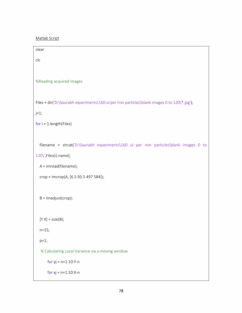
78

Matlab Script

clear

clc

%Reading acquired images

Files = dir('D:\Saurabh experiments\160 ul per min particles\blank images 0 to 120\*.jpg');

j=1;

for i = 1:length(Files)

filename = strcat('D:\Saurabh experiments\160 ul per min particles\blank images 0 to

120\',Files(i).name);

A = imread(filename);

crop = imcrop(A, [6.5 93.5 497 584]);

B = imadjust(crop);

[Y X] = size(B);

n=15;

p=1;

% Calculating Local Variance via a moving window

for yj = n+1:10:Y-n

for xj = n+1:10:X-n

79

C = B(yj-n:yj+n, xj-n:xj+n);

D = reshape(C,[1,(((2*n)+1)*((2*n)+1))]);

F = double(D);

LV(p) = var(F);

p=p+1;

clear C D F;

end

end

% Calculating Global Variance

GV(j) = var(LV);

j=j+1;

end

80

APPENDIX D MATLAB SCRIPT FOR MEASUREMENT OF PARTICLE

VELOCITY

Matlab script

clear

clc

fps = 10000/3;

widthpix = 688;

% Reading acquired images

Files = dir('D:\Saurabh experiments\p19\*.jpg');

j=1;

for i = 1:3:length(Files)

filename = strcat('D:\Saurabh experiments\p19\',Files(i).name);

A = imread(filename);

C = imadjust(A);

% Circle detection command

81

[centres, radii] = imfindcircles(C,[22 50],'objectpolarity','dark','sensitivity',0.88);

TF = isempty(centres);

if TF == 1

errordlg('no circle detected')

else

% Storing detected circle centre values in suceessive frames

D=sortrows(centres,-1);

E(j,:) = D(1,:);

F(j) = 2 * radii(1);

j = j+1;

clearvars centres radii D TF;

end

end

82

m=1;

for k = 1:j-2;

% particle movement between two successive frames

X(k) = E(k,1) - E(k+1,1) ;

Y(k) = E(k,2) - E(k+1,2) ;

Z(k) = (X(k)^2 + Y(k)^2)^0.5 ;

% velocity and distance from inner wall of a particle

width(m) = (727 - E(k,2))*(290/widthpix);

dist(m) = (Z(k)*290)/widthpix;

vel(m) = dist(m) * fps * 0.000001;

m = m+1;

end

% average velocity of particle

avgvel = mean(vel)

avgwidth = mean(width)

avgdia = mean(F) * (290/widthpix)

83

REFERENCES

[1] G. Segre and A. Silberberg, "Radial Particle Displacements in Poiseuille Flow of Suspensions,"

Nature, 1961.

[2] S. Rubinov and J. Keller, "The transverse force on a spinning sphere moving in a viscous,"

Journal of Fluid Mechanics, 1961.

[3] P. Saffman, "The lift on a small sphere in a slow shear flow," journal of fluid Mechancis, 1965.

[4] B. Ho and L. Leal, "Inertial migration of rigid spheres in two-dimensional unidirectional

flows," Journal of Fluid Mechanics, 1974.

[5] P. Vasseur and R. Cox, "The lateral migration of a spherical particle in two-dimensional shear

flows," Journal of Fluid mechanics, 1989.

[6] J. Schonberg and E. Hinch, "Inertial migration of a sphere in Poiseuille flow," Journal of Fluid

Mechanics, 1989.

[7] E. Asmolov, "The inertial lift on a spherical particle in a plane Poiseuille flow at large channel

Reynolds number," Journal of Fluid Mechanics, 1999.

[8] J. Feng, H. Hu and D. Joseph, "Direct Simulation of Initial Value Problems for the motion of

Solid Bodies in a Newtonian Fluid," Journal of Fluid Mechanics, 1994.

84

[9] D. Carlo, "Inertial Microfluidics," Lab on a Chip, 2009.

[10] J. Zhou and I. Papautski, "Fundamentals of inertial focusing in microchannels," Lab on a Chip,

2013.

[11] D. Carlo, D. Irimia, R. Tompkins and M. Toner, "Continuous inertial focusing, ordering, and

separation of particles in microchannels," PNAS, 2007.

[12] S. Kuntaegowdanahalli, A. Bhagat, G. Kumar and I. Papautski, "Inertial microfluidics for

continuous particle separation in spiral microchannels," Lab on a Chip, 2009.

[13] N. Pamme, J. Eijkel and A. Manz, "On-chip free-flow magnetophoresis: Separation and

detection of mixtures of magnetic particles in continuous flow," Journal of Magnetism and

Magnetic Materials.

[14] P. Gascoyne and J. Vykoukal, "Particle separation by dielectrophoresis," NIH, 2002.

[15] F. Bretherton, "The motion of rigid particles in a shear flow at low Reynolds number,"

Journal of Fluid Mechanics, 1962.

[16] J. Matas, J. Morris and E. Guazzelli, "Lateral Forces on a Sphere," 2004.

[17] J. Martel and M. Toner, "Particle Focusing in Curved Microfluidic Channels," Nature, 2013.

measurement of slip velocity and lift coefficient for

Documents