AERODYNAMIC PRELIMINARY ANALYSIS SYSTEN I1

PART I THEORY

By E. Bonner, W. Clever, K. I?unn

North American Aircraft Division, Rockwell International

An aerodynamic analysis system based on potential theory with edge con- sideration at subsonic/supersonic speeds and impact type finite element solutions at hypersonic conditions is described. urations having multiple non-planar surfaces of arbitrary planform and bodies of non-circular contour may be analyzed. tudinal and lateral-directional characteristics may be generated.

Three-dimensional config-

Static, rotary, and control longi-

The analysis has been implemented on a time sharing system in conjunc- tion with an input tablet digitizer and an interactive graphics input/output display and editing terminal to maximize its responsiveness to the preliminary analysis problem. CDC 175 computation time of 45 CPU seconds/Mach number at subsonic-supersonic speeds and 1 CPU second/Mach number/attitude at hyper- sonic cmditions for a typical simulation indicates that program provides an efficient analysis for systematically performing various aerodynamic config- uration tradeoff and evaluation studies.

i

https://ntrs.nasa.gov/search.jsp?R=19810012500 2018-08-28T21:55:42+00:00Z

TABLE OF CONTENTS

INTRODUCTION

LIST OF SYMBOLS

SUBSONIC/SUPERSONIC

Body Solution

Surface Solution

Aerodynamic Characteristics

Drag Analysis

HYPERSONIC

Aerodynamic Characteristics

CONCLUSIONS

REFERENCES

APPENDIX A SUBSONIC/SUPEEDNIC FINITE ELB/IENT DERIVATIONS

APPENDIX B SU'RFACE EDGE FORCES

APPENDIX C HYPERSONIC FINITE ELEMENT ANALYSIS

Page

1

2

7

9

20

33

40

59

61

64

65

68

86

102

ii

INTRODUCTION

Aerodynamic numerical analysis has developed t o a point where evaluation of c q l e t e a i rcraf t configurations by a single program is possible. grams designed for th i s purpose in fact currently exist , but are limited i n scope and abound with subtleties requiring the user t o be highly experienced. Many of the diff icul t ies are attributable t o the numerical sensit ivity of the associated solution. In preliminary design stages, some degree of appro- ximation is acceptable in the interest of m o d e s t turn-around time, reduced computational costs simplification of input and s tabi l i ty and generality of results. The importance of short elapsed time stems from the necessity t o systematically survey a large number of candidate advanced configurations or major component geunetric parameters i n a timely manner. Modest computa- tional cost allows a greater number of configuraticns and/or conditions t o be eca-i anically investigated.

Pro-

One approach i n th i s sp i r i t is to employ panel approximaticns which reduce the member of simultaneous equations required t o sat isfy flow born- dary conditions. crossflow body solutions and non-interfering panel simplifications are exam- ples of approximations which can be used for this purpose.

Surface chord plane formulatims, locally two dimensional

Finite element analysis when combined with rea l i s t lc assessment of l i m i - t a t i m s and esgimated viscous characteristics provides a valuable tool for analyzing general a i rcraf t configurations and aerodynamic interactions a t modest attitudes for subsonic/supersonic speeds and evaluation of compressible nm-linearit ies at high Mach numbers.

LIST OF SWi3OLS

A

Ai j

b

C

e

Projected oblique cross section area

Influence coefficient. to vortex panel j of unit strength

Yomalxash a< control point i due

Area of quadrilateral panel i

Reference span

Local chord

Reference chord

Average chord

Section drag coefzicient

Drag coefficient

Flat plate skb- friction coefficient

Boundary ccndition for control Doint i

Section lift coefficient

Rolling, pitching and yawing moment coefficients

Lift coefficient

.. -

.. -. - Section normal force coefficient

Pressure coefficimt (P-pa) /q

Net pressure coefficient [PpI;-Pu!/q and vortex panel strength

Axial,side,normal force coefficient

2

LIST OF STIBOLS ( C O N T I W )

C*

P

P r

Force components

.Axispimetric outer solution to potential equation

Radius of curvature of cross sectional boundary

Unit vectors i n x,y,z direction respectively-

Drag due to l i f t factor or skin friction thickness correction factor

Equivalent distributed sand gain height or attainable suction fraction

Effective length

Length of segment i, i+l of contour C n

Equivalent body length o r geometric length

Body fineness ratio

Mach number

Moment components

Unit normal

Rolling, pitching and yawing velocity about x9 y anci z

Xondimensional angular velocities pb/ZU, qE/3U and rb/ZU

Pressure

Prandtl number

3

LIST OF SYMBOLS (COhT14yuED)

cl Free stream dynamic pressure 1/2&

Recovery factor r

U n i t Remolds number o r radius of curvature

Repolds number based on [ 3

R

Gas constant b?

Segment arc length S

Body cross sectional area o r surface area S

Reference area

Static temperature -OR o r tangent of quadrilateral panel # leading edge sweep

T

Airfoil thichess ra t io

x,y,z nondimensional components of perturbation velocity U,V,hi

U Freestream velocity

Je t velocity

Complex, potential function

Body axis coordinate system

Cylindrical coordinate system

Complex number y+iz Z

Angle of attack a

Local angle of attack at surface control point i

h g l e of sideslip o r Jm

4

LIST OF SYX3OLS (COit”rI?jcIED)

rl

8 A ’

LI

v

P

T

cp

4

+ n

Sub scr ipt

C

CG

F

R

Vorticity strength per unit length or ra t io of specific heats

Horseshoe vortex strength in Trefftz plane

Deflection o r impact angle

Lateral surface coordinate

Body slope

Dihedral angle of quadrilateral panel o r boundary layer momentum thichess

Sweep angle Absolute viscosity

h e m a t i c viscosity, p/ p

Dens ifqy

Source density

Side edge rotation factor

Perturbation veloc ty potential

Total velocity potential

See figure 3

Leading edge rotation factor

camber

center of gravity

friction

lower surface

5

LIST OF SYMBOLS (CONTINUED)

LE

r

t

T

TRAN

U

V

W

to

Superscripts

1

f f

*

leading edge

recovery

thickness

tip

transition point

upper surface

vortex

wave

freestream condition

first derivative or quantity based on effective origin

Second derivative

Eckert reference temperature condition

6

SUBSONIC/SUPERSCNIC

The arbitrary configurations which may be treated by the analy are siiiated by a distribution of source md'mrtex s-hgularities . Each of these singularities satisfies the linearized small. perturbation potential equation of motion

The singularity strengths are obtained by satisfying the condition that the flow is tangent to the local surface:

a5 a- - t o

All of the resulting velocities and pressures throughout the flow may be obtained when the singularity strengths are known. A configuration is c q o s e d of bodies, interference shells and aerodynamic surfaces(wings, canards tails etc -1. The following types of singularites are used to represent each.

wing and vertical tail

- chord plane source and vortex panels -

?t

fuselage q d nacelles -sxface source line segments-

interference shell -vortex panels -

The first step in the solution procedure consists of obtaining the strengths of the singularities simulating the fuselage and nacelles, froin r. isolated body solution. The present analysis uses slender-body theory to

predict the surface and near field properties. The solution is composed of a compressible axisynnnetric component for a body of revolution of the same crossectional area and an incompressible crossflow component, 9 ?

satisfying the local three dimensional boundary' conditions in the ( y , ~ ) plane. The crossflow is a solution of Laplace's equation

.A two-dimensional surface source distribution formulation is used to obtain this solution. When the body singularity strengths are determined, the perturbation velocities which they induce on the aerodynamic surfaces, or other regions of the field, are evaluated.

- ( . The assumptions of thin airfoil theory allow the effects of thickness

and lift on aerodynamic surfaces to be considered independently. the effects of the aerodynamic surfaces can be simulated by source and vortex singularities accounting for the effects of thickness and lift, respectively. The source and vortex distributim used in this program are in the form of quadrilateral panels having a constant source or vortex strength. The vortex panels have a system of trailing vorticies extending undeflected to downstream infinity. varying source panel is provided as an option to elmate singularities associated with sonic panel edges at supersonic Mach numbers. The panels are planar, that is they have no incidence to the free stream (although dihedral may be included), since thin airfoil theory allows the transfer of the singularities and boundary conditions to the plane of the mean chord. 'fhese boundary conditions are satisfied at a single control point on each panel. centroid while the effects of twist, camber, and angle of attxk are satisfied at the spanwise centroid of each vortex panel and at 8 7 . 5 percent of its chord.

Therefore,

The use of a chordwise linearly

For thickness,the control point is located at the panel

- - - -

.4 cylindrical, non-circular, interference shell, composed entirely of vortex panels, is used to account for the interference effects of the aerodynamic surfaces on the fuselage and nacelles. on an interference shell are such that the velocity normal to the shell induced by all singularities, except those ofthe body which it surrounds, is zero. for vortex panels.

The boundary conditions

The boundary conditions are satisfied at the usual control points

The following sections define the details of the solution procedure. Included are discussions o f the isolated body analysis, surface finite element analysis considering edge effects, and evaluation of aerodynamic characteristics including drag. interested in further pursuing a particular point.

References are cited far the reader

8

BODY SOLUTION

According t o slender body theory' 2 the flow disturbance near a sufficiently regular three-dimensional body may be represented by a perturbation potential of the form

9 * Q ( y , r ; x > * gCx1 (13

Qc%ZirO is a solution of the 2-D Laplace equation in the y, z cross flow plane satisfying the following boundary conditions

v + = j v + h = o

C(x) and n, are defined in figure 1 . A general solution for 8 may be written as the real part of a complex potential function W(2) with Z = y + i z .

b

8 = R, W = rZ( A,w L Z + 2 A-(x) Z - m ) crC. I

A useful alternative representation of 9 and W is obtainable with the aid 3 of Green ' s tkeorem.

9 = R,w - - 2 R p f b C 3 ) L ( Z - 3 ) d A (3

where a(3) is a ''source" density fo r values of 'I = yc + i zc , (yC,zc) being .coordinates of a point on the contour c(x) .

The function g(x) is obtained by matching (0 of equation (1) which is valid i n the neighborhood of the body with an appropriate "outer" solution. g(x) is then found to depend explicitly on the Wch numb-er W and longitudinal variation of cross -sectional areas S (x)

where

9

Figure 1. Body Slope and Cross-sectional Variables

10

The body axis perturbation velocities are obtained by differentiation of equation (1)

A t supersonic speeds, -zone of influence considerations require that u = v = w 0 for x-pr c o .

Solution of the preceding equations is based on an extension of the method of reference 3.

CROSS FLOW COMPONENT

The reduction of computations to a numerical procedure utilizes the integral representation of + given in equation (3) by &screrization of the cross sectional boundary into a large number of short linear segments (figure 2) over each of which the source density 6 3 value determined by bounhry conditions.

is as.smed cons.tant at

Computation of a(i,n) over the segment i, i41 proceeds by applying a .. the boundary condition equation ( 2 ) at each segment of Cn. represents the velocity vector, the corresponding complex velocity in the cross flow plane is obtained by differentiation of W in equation (3 ) with respect to Z:

If vq=q=jv+kw

The contribution by the sources located on segment i, i+l to the velocity at P; ,n is first evaluated. with respect to the horizontal axis, we have

Noting that i, i+l makes an angle e(i ,n)

i e( L, - ) a3 = dAc.2

and the contribution to the integral in equation ( 5 ) may be written:

11

Figure 2. Cross-section Bouiidary Segmenting Scheme

12

.After integration of the last tern and summation over all contributing segments, the result may be written

in which, referring to figure 3 , the quantities R(i,j,n) and &(i,j,n) are defined by the relationships

To insure uniqueness of the complex velocity, care must be exercised in assigning values to the angles figure axis so that when facing from Pi,n to Pi+l,n , a point p, ,n jFt to the left of i,i+l shall define an angle Y(i,j,n) = S(i,n). As Pj?n traverses a path around Pi,n t o a point just to the right of i,i+l, U(i, j ,n) increases from 8(i,n) to e(i,n) +2n . as ?j ,n traverses a path around Pi+l,n. In consequence of these definitions d (i,j ,n) becomes -T when approaching i,i+l from the right and T when approaching from the left. *he stream fwction upon traversing any closed path which encloses a distributim of finite sources.

(i, j ,n) and ?xi, j ,n) . Referring to 3 , these are measured counter-clockwise from the positive y

The same holds true for 9 (i,j ,n)

This discontinuity reflects that exhibited by

From the boundary condition equation ( 2 ) , we have

After substitution of v and w from equation (6 ), this last e,qression becomes

where

13

Figure 3. Details of Variables Pertaining t o Segment i,i+l of BOUII~ZKY Cn

14

The surface normal perturbation velocity - (a8A-I. of the body slope ( a y h x ) ~ rrc , the angles of at;';ck 4 , and sideslip p and the angular velocities p,q,u as

may be written in tenns

Satisfying equation 7 boundary yields a set of equations for d (i,n) . at each of the points 3, ,n on a given contour

AXISYMMETRIC COMPONENT

Differentiation of g(x) must be carried out with due concern for the nature of the improper integrals appearing in equation (4). The result is

where I E L - I

15

To compute the second derivatives of the equivalent body cross sectional area required for g'(x> ,the first derivatives at 5& are found by finite differences between and %+I. Second derivatives Sf'(&$ at F m C%++l + &%)/2 are then found by finite differences between *S' at and %+I. between k and 2 m+l.

e. Finally S"(xrn) is detennined by linear interpolation of St'(5$J

' PERTORBATION VELOCITIES

The axial velocity u depends on (W/ax) and the axisymmetric solution g' (x). ( W / a x ) is obtained by differentiation of the integral in equation ( 3 ) to first obtain an exact expression which is then approximated by evaluating the result over the segmented boundav.

.

The derivation of 3413~ must take into account the fact that the path of integration in equation (3 ) is a function of x. figure 1 by d( ) and increments taken normal to e are denoted by 6 ( ) . tion of equation (3) then yields

Referring to increments of a dependent variable taken along C(x) are denoted

Differentia-

From figure i

where h(S) is the radius of curvature of C(x) at from figure I

3 . In addition, we have

16

To evaluate - dc3- we note, S X

&e s i

Introducing equations ( 9 ) , ( 1 0

- =

Again, assuming that quantities i n the brackets of the integrands are constant over i ,i+l,

where

17

The radius of curvature h(i,n) and the derivatives &a-/bx , S y / g x are approximated at the mid points of the segments i,i+l as follows

a) &C/ Sx - the derivative at the idd-point 2 n of the interval xn,xn+l is set equal t o the divided difference between d (i,n) and b(i,n+l) . Linear interpolation between these derivatives then yields &/dx at Xn.

b) v / s % - referring to figure 4 , the displacement 8 7 is determined by linear interpolation between and d 3 i+l,n. b 7/(xn+1 - Xn) then represents 97/,/Sx at the stations x'n then yields bg/Sx at Xn .

Linear interpolation between

c) l/h: - 43 at Pi,n is determined by interpolation between values of 8 (i,n) at 5 i,n. The curvature l/h at i,n is then set equal to the divided difference between B at Pi+l,-, and B at Pi,n.

obtained from The lateral and vertical perturbation velocities, V and ~3 , are

Integration over the boundary with constant segment source density yields:

Thus

18

i,n

Figure 4. Interpolation Procedure f o r Detemination of ( b d s x )i,n

19

SURFACE SOLUTION

The wing, canard, vertical and horizontal tail are simulated by a system of swept tapered chord plane source and vortex panels with two edges parallel t o the free stream. The coordinates of the panel corners are specified with respect to an (x,y,z) system having its x axis in the free stream direction and its z a x i s i n the l if t direction. influence equations are written in terms of a coordinate system having a z axis normal t o the panel and an x axis along one of the two parallel edges. A coordinate transformation is necessary t o obtain the coordinates in the panel reference system. If the plane of the panel is inclinded a t an angle with respect t o the y, z plane, a transformation in to the panel coordinate system (xp ,yp, zp) is accomplished as follows :

The Panel

x, = x

control

panel point

(*c, SL > ?,I

A transformation of the (up,vP,wp) velocities into the coordinate system of the panel on which the coatrol point is located (uc,vC,wc) results i n the axial, binormal and normal velocities induced on the panel.

For the image of the influencing panel, the signs of y , 6, and vc are changed while using the same calculation procedure.

20

PANEL SINGULARITY STRENGTHS

The source singularity strengths may be found directly by equating each source panel strength t o the slope of the thickness distribution a t its control point. For panel i

de*! Q-i = ( q - j ;

where Z t refers t o the shape of the thickness distribution. equa.tions for the source panels can then be used t o obtain the velocities induced by the source panels anywhere in the flow.

The influence

The determination of the vortex panel singularity strengths are the final step in the solution procedure. of simultaneous equations utilizing the vortex panel influence equations t o relate the singularity strengths t o the boundary conditions a t the control points of the vortex panels. The boundary conditions permit the condition of tangential flow to be satisfied.

They are obtained by solving a set

Each vortex panel j having singularity strength CP; induces a set on panel i. of velocities ( ~ 7 ~ . A:~.~ A?.

equations can be mi t ten . Therefore a s e t of influence

‘4

d e . =

where ( w i , vo2, viGj) refer to the velocities induced by a l l other body and source singularlties, and written in the coordinate system of the panel containing the control point. Since the resultant velocity along the normal a t a panel control point m u s t be zero,

21

and the following system of equations results

This set of linear equations can be solved for the CP. and, since it assumes symmetrical panel loading, can be used to dethmine the longitudinal characteristics. the lateral/directional characteristics. panel loading and has a correspondingly different set of influence coefficients Aij .

A similar set of equations exist for the calculation of This set assumes an antisymmetrical

BOUNDARY CONDITIONS

Several types of basic and unit boundary conditions are considered Linearized and can be classified as either symmetric or antisymmetric.

theory allows the superposition of these basic unit solutions. and r rotary derivative boundary conditions are the result of placing the configuration at oc* 0, p= 0 in a flow field rotating at one radian per second.

The p, q .

Symetric :

1) basic (A*/&) - a0 - we 0 5

( d z J d x > = d a c e slope due to twist and camber

Go = normalwash induced by slender body thidcness and camber 0

= normalwash _. induced - by source panels _- wo 5

22

1

3) Unit q mtation

4) unit Rap

AIl-tTic:

1) Unit beta

2) Unit p mtation

3) ~t r rotatAm

4) Unit flap

7I- - - r IBO

= 1. for Rap panel

- normdlwash in&cd by slender body P e at unit sideslip

aR -wash induced by slender bocly 0 undergoing unit r rotation

- G ?r 100

= 1. f o r flap panel

= 0. for others

23

CONSTANT SOURCE AND CONSTANT VORTICITY PANEL INFLUENCE EQUATIONS

The source f in i t e elements have a discontinuity in normal velocity across the panel surface while the vortex f in i t e elements have a discontinuity in the tangential velocity in a direction normal t o the panel leading edge. of the discontinuity, i n each case, is constant over the panel area. the vortex panels have a system of t ra i l ing vorticies extending undeflected t c doms tream infinity .

The magnit In addition

-4. constant pressure o r constant source panel Fiith a quadrilateral shape can be constructkd by adding o r subtracting four semi-infinite triangular shaped pane&. These semi-infinite triangles, each determined by a corner of the quadrilateral, can be assumed t o induce a velocity perturbation every- where in the flow. and a l l four corners must be included t o make any sense.

However, each corner represents only an integration l i m i t ,

t

x

I

If it is kept in mind that four corners must be included, one of these triangles having sides determined by y = 0 and x-Ty = 0, induces the following perturbation velocities:

24

constant source panel

25 I

The total. panel sol.ution is built up by combining each of the four corners

e tc .

These results hold for both subsonic and supersonic free stream velocities. In the l a t t e r case, only the real (downstream) contributi0E.s are considered.

The perturbatior, potential expressions are derived in Appendix A. Sub- sequently ,verif icati-on of the perturbation velocities is presented.

26

L I h i Y VARYING SOURCE PANEL INFLUETKE EQUATIONS

In supersmic flow constant source panels having a sonic edge have a real singularity along an extension of this edge. because :

The singularity occurs

I 1

* .

Control points which are near the extension of this edge will have large u and v velocities induced upon them. using panels which have a source distribution which varies linearly in the chordwise direction. The resulting continuous source distribution eliminates the singula ies. The linearly varying source panel influence equations can be found by integrating the constant source panel influence equations with respect to x.

The singularity can be eliminated by

These Trelccity components satisfy the same criteria as the velocity components for the constant source panels except that the source strength is proportional to x-Ty. The source panel finite elements are constructed with the following properties.

27

1. A l l panel leading and ti-ailing edges are a t constant (21, side edges are a t constant y.

2 . Each source f in i te element is c q o s e d of a pair of chordwise adjacent panels *

3. The source strength varies linearly with chord measured from the leading edge of a panel pair, i.e. the maximum value of the source strength is proportional to the loca l chord and attains this maximum on the! panel edge joining the panel pair.

% i ?he perturbation velocities induced by this panel pair are composed of contributions from six' corners.

If there are ?: panels in <.he chordwise direction there w i l l be if-1 singularities o r whmn source strengths associated with them. n e linear variation ir, the source distribution means the value of d=/dx amst be zertj a t the leading and trailing edg5s of each span s ta t i on . This may be ZI &?desired restriction and therefore tne use of Linesrly varying smrce paneis is optioml.

28

EDGE EFFECTS

The low pressure created by high velocities around a surface subsonic hading edge results in a suction force. As the edge becomes thinner o r the angle of attack increases, the flow deviates from potential conditions resulting in a progressive loss of theoretical suction and an increase in drag. Generalizing a concept due to PolharrmS5, it is assumed that the leading edge vortex created by the detached flow in effect rotates the lo s t suction force perpendicular t o the local surface.

In order to implement th i s philosophy, a method of determining the spanwise variation of potential suction was developed using linear thin wing theory and involves finding the coefficient of the 1/~;i. term in the chordwise net pressure distribution. of arbitrary planform in the presence of bodies a t any Mach number.

The analysis is applicable to multiple surface problems If the

chordwise net-pressure distribution on a thin wing a t any given span station is expanded in a series

N

i t . i s shown in appendix B that the leading edge nondimensionalized suction force per unit length is

where T = L A , . , .

and c is the local chord

Only the first term in equation 1 2 contributes t o the thrust, since it is If the chordwise the only contribution which is inf ini te a t the leading edge.

pressures are known a t M points along the chord, the coefficients A, are obtained by f i t t i n g a least square error curve described by N terms of the series, through the points, where N < M. obtained using constant pressure panel analysis.

The pressure distribution is

29

The method used t o compute the suction force a t surface t ips is similar to t h a t for the leading edge. flow, it is shown in appendix B that the t i p suction force is:

By using the .irrotational property of the

where

cr surface average chord

t i p chord

t i p surface la te ra l surface dimension

faction of chord

is local section normal force coefficient

and as 7- 7,,,px the net pressure coefficient is assumed t o be of the form

30

The sectional leading edge suction attained in the real flow, estimated by6

N

= 5 q ) = L(+LJ-l +p$ l

where

and

31

The chord of the normal section, C,

associated leading edge radius is designated by rn

is defined so as to place the maximum ss, t .9 a t the mid chord as indicated i n the following sketch, The

Leading

/ Edge

Potential t i p suction is assumed to be fully rotated as a result of vortex formatkn in the present analysis.

32

AERODYNAMIC (=HARACTERISTICS

Longitudinal and lateral-directional forces and moments due to thick- ness, twist and camber, pitch, sideslip, and the dimensionless rotary velocities 8 , q, and.? are obtained from surface pressure integrations of the various configuration components . BODIES

The pressure coefficient, to an approximation consistant with slender body theory, is

The forces and moments are obtained from the surface integrations

33

In terms of these expressions, the commonly used aerodynamic coefficients are

where L is the body length and E , b and Sref are configuration reference chord, span and area,respectively.

34

Crosscoupling between the pitch, sideslip, and rotary motions through - the’ product and quadratic te- in - - equation -(20) -is neglected.

PLANAR COMPONENTS

Surface pressure distributions are calculated for planar components using the first-order linearized form ’

z u =-q;,Ne t ‘%ET -1 c P = - - U 4

The +/- signs refer to the upper and lower surfaces respectively.

other vortex and source panels.

The term

These velocities are obtained by multiply- consists of the velocities induced by the isolated bodies and J u 1 - 0

-~ ing the $ influence mairices by the appropriate panel strengths. c p ~ s y & tern accounts for the 3

I’he perturbation velocity induced by the . -

local distribution of vorticity and changes sign from upper to lower surface. combinations of a l l the basic and unit solutions.

The total $- and ‘?NET values are the result of taking linear

The net pressures for each of the basic and unit solutions are integrated numerically to give the section forces and moments, component forces and moments, and configuration forces and moments.

Since the vortex panels have a constant pressure distribution, a block integration s&ene is employed. and unit force and moment coefficients are combined in a linear manner to produce the aerodynamic characteristics for any desired flight condition. Since drag varies in a parabolic manner, it must be considered on a point by point basis as defined in a later section.

With the exception of drag, these basic

The longitudinal normal force distribution on the bodies for each solution. The lead distrihtion on the interference of the body is given by integrating over all vortex panels at longitudinal station.

normal force

is calculated shell portion a given

35

where N is the number of panels around the shell, body,bX is the length of the interference area, and Ci = 2 for a centerline body or C 1 = 1 for an off centerline body. This carryover load distribution is added to the previously calculated isolated body lcngittdinal load distribution.

L is the length of the shell segment, A,is the panel

The section characteristics of planar components are determined by a chordwise summation of panel data at each span station and are given by the following equations:

local n o m 1 force

weighted normal force

weighted lift force

cencer of pressure

where N,is the number of chordwise panels, and As is the width of the span station and is given by

36

~~~~~s including edge vortex effects are given

side force

ro li ing moment

pitching moment

37

yawing moment

where N is tlhe number of vortex panels on half of a s y e t r i c a l coqonent (or total for an S Y e t r i c d CDFOnent) and F1, F2 are given by

symetric loading

antisymmetric loading .

F1 = 1 = 2

Fz = 1 = o

F1 = 1 = o

F2 = 1 = 2

asymmetric geometry symmetric geometry asymmetric geometry symetr ic geometry

asymmetric geometv symmetric geometry asymetric geometry symetric geometr;

For the leading and side edge vortex terms, Ns is the to t a l number of spanwise panels for both component halves, NCT is the number of t i p chordwise anels, XTQ is the axial location of t i p vortex center of pressure, As' = AS F - 2 1 + T and the rotation factors S a n d T are derived in appendix B and defined.below.

Leading edge vortex rotation:

where d is the slope angle of the leading edge camber l ine and Vile sign of coefficient A,(from equation 13) is used t o determine the direction o f vortex rotation.

38

Side edge vortex rotation:

where 6 is the slope angle of the t i p camber line, 5 is plus for the l e f t side and negative for the right side of the configuration and the sign of coefficient Cns, (from equation 1 4 ) is used t o determine the direction of vortex rotation.

The ;Y coordinate of the center of pressure is given by

For interference shell components, the total forces and moments of the corresponding isolated body are added t o those of the shell.

The forces and moments for the complete configmaticin are obtained by sumning those of the indivLdual components.

39

DRAG ANALYSIS

Estimation of configuration aerodynamic efficiency requires the calculation of drag. friction and pressure drag components that are assumed to be tndependent of each other. parabolic polars a s a result of the incorporation of attainable suction considerations.

The analysis separates the computation into skin-

The following form is considered and produces non-

+ c, + c o WAVE ORSE

+ CD VI SCOLIS

C D = c o L I F T

The specific techniques used for the various drag evaluations are discussed below.

SKIN FRICTION d

Several wll established semiempirical techniques for the evaluation of adiabatic laminar and turbulent f l a t plate skin friction a t incompressible and compressible qeeds are used t o estimate the viscous drag of advanced aircraft using a component buildup approach.. A specified transition point calculation option is provided i n conjunction with a matching of the momentum thickness t o link the two boundary layer states. turbulent condition, the increase in drag due t o distribuzed surface roughness is treated using unforrnly distributed sand g r a i ~ results. Component tAhickness effects are apprcxci-nated using e-xperimental data correlatiors f c r two-dimensional a i r fc i l sections and bodies of revolution.

For the

Considerations such as separation, component interference, and discrete protuberances [e.g. antennas, drains, a f t facing steps, etc.) aut be accounted for separately if present.

40

In the following, a discussion is presented for a single component evaluation i n order t o simplify writing of the equations and eliminate multiple subscripting. The total result is obtained by a surface area weighted summation of the various component analyses as described on page 6 3 .

Laminar/Transit ion

A specified transition option is provided in the program. The principal function of the calculation is t o provide the conditions required to ini t ia l ize the turbulent solution. length and momentum thickness Reynolds numbers are required.

In particular, the transition point

where

This solution is based on the laminar Blasius result in conjunction with Eckert Is compressibility transformationY. This option permits an assessment of the reduction in skin-friction drag if laminar flow can be maintained for the specified extent. establish the liklihood that such a condition w i l l be realized i n practice o r t o w h a t extent.

@, chapter 121)

I t does not

41

Turbulent

Smooth and distributed rough surface o?tions have been provided in the analysis. momentum thickness a t the transition point produced by the laminar/transition solution. origin) is established fo r the turbulent analysis.

In either case, the solution is init ialized by matching the

That is , an effective origin (cawnonly referred t o as a virtual

For the hydraulically smooth case

A X -

CF from equation (21) ,for known c,RdOx

42

where

I- = 0 . 8 8

d = 0.76

The compressible turbulent f l a t plate method used here i s that proposed by Van Driest1° conjunction with the Squire-Young formulation for profile drag ( 8 , chapter XXIV) as applied t o a f l a t plate.

based on the Von Karman mixing length hypothesis i n

43

For the distributed rough case

TIC*IJ AX, = x

- 2.5 y-l z -' = 1.89 i 1.62 1 ( I + ?" M - )

%

The turbulent f l a t plate method used here is that of Schlicting [B, chapter XXI) which i s based on a transposition of Nikuradse's densely packed sand grain roughened pipe data. due to the rechcticn in density a t the wall as proposed by Goddard!' The selection of the equivalent smd grain rcughness for a given manufac- turing surface finish is made with the aid of Table I1 which was taken from Clutter! 2

The effect of compressibility is

44

TABLE I1

Aerodynamically smooth

Polished metal or wood

Natural sheet metal

Smooth matte paint, carefully applied

Standard camouflage paint, average application

Camouflage paint, mass-production spray

Dip-galvanized metal surface

Natural surface of cast iron

Equivalent Sand Roughness 5s (inches)

0

0.02 - 0.08

0.16 10-3

0.25 x 10-3

0.40

1.20

6 x

10 10-3

Thichess Corrections

The foregoing evaluations produce as estimate of the shearing forces

aft has a non vanishing thickness, an estimate of pressure (at zero angle of attack) for a variety of conditions. As

gradient effects on skin friction and boundary layer displacement pressure drag losses is required. one which will be used here is based on non-lifting experimental correlations for symmetric two-dimensional airfoils and axisymmetric bodies. The following relations derived by Horner (1 3, chapter VI) are used, respectively.

A common procedure for accomplishing this and the

4 t 1 * K, c + L o ( $ )

a " J, Cn d a = - = I + I . S ( i ) + 7(i) Car

45

Homer reccmends K,= 2 fo r s i r fo i l s x i t h ;na~l?;lc~?1 th ichess a t 502 chord and S i = 1 . 2 f o r ?:4CA. 61 and 55 sa-ies airsoils. In -this rezard, t he best infomation available t o an ana1;rst for h i s particular contcur shculc! be used. as the sqe rc r i t i ca l a i r foi l , etc.

This i s espcciall:; tzxe f o r niodern high performance shapes siich

Total Viscoas Drzg

The aircraft total viscous-drag coefficient is estimated by a sum of the preceding analysis over a11 components ( i . e. wing, fuselage, vertical t a i l , etc.) . T'nat is

The component length used in the calmlation of the skin friction coefficient is the mean chord f o r planar component segments and the physical length f o r bodies and nacelles. -

BASE DRAG

Blunt base increments are estimated at subsonic and supersonic speeds by

where

0.064- t 0.042 (M,- 3.84) 2 '7-2 I

The expressions for the base pressure coefficient are derived from correlation of flight test results for the X-15, various lifting bodies, and the space shuttle. analysis.

Power effects are treated as reductions in base area in the present

46

One hundred percent suction drag due t o l i f t and supersonic wave cirag due t o thickness can be evaluated by integration of the mnentum flm through a large circular cylinder centered on the x a x i s and whose radius approaches infinity.

The resulting expression f o r the to t a l pressure drag is as f o l l m s :

47

Vortex Drag

The vortex drag may be computed when the distribution of t ra i l ing vorticity in the Trefftz plane is horn. wing theory result in a vortex sheet which extends directly downstream of a l l l i f t i ng surfaces. a l ine integral over the vortex sheet in the Trefftz plane the following expressions for l i f t and drag result .

The assumptions of linearized thin

By changing a surface integral for kinetic energy t o

I C

C

where

C vortex sheet branches

=, weighted section normal force coefficient c T c /cAU -

urn asymptotic normal velocity on the vortex sheet

vortex sheet branch coordinate 7

8 inclination of vortex sheet with respect t o y axis

48

velocity on the vo of firrite trailing horseshoe ' t o the local section Cn(S)e The

normdj velocity is computed a t a control point located midway between the

control point i

Eachvurtex j induces section i.

a contribution t o the noma1 velocity at

Theref ore

49

The integral for wave drag

may be simplified by allowing the cylb-drical surface of integration t o recede infinitely far fr& the disturbance. Under these conditions, the spatial singularity simulations can be reduced to a series of one- dimensional distributions. The basis for this reduction is the finding by Hayes (14) that the potential and the gradients of interest induced by a singularity along an arbitrary trace on a distant control surface, say PP' of figure 6 (or alternately described by the cylindrical angle e), is invariant t o a finite translation along the surface of a hyperboloid emanating from the trace and passing through the singularity. As the apex of the hyperboloid is a great distance away, the aforementioned movement is along a surface which is essentially plane; it will be henceforth referred to as an "oblique plane". differential equation, all singular solutions which lie on the surface of the same hyperboloid (oblique plane) may thus be grouped to form a single equi- valent point singularity whose strength is equal to the algebraic sum of the individual strengths and which induces the same potential (momentum) along the trace as the group of individual singularities.

Since a singularity is a solution of a linear

This finding provides the basic technique for reducing a general spatial distribution of singularities to a series of equivalent lineal distributions. This is accomplished by surveying the three-dimensional distribution longi- tudinally at a series of fixed cylindrical angles, e . survey produces an equivalent lineal distribution by systematically cutting the spatial distribution at a series of longitudinal stations along its length. along the "oblique plane" t o form one of the equivalent point singularities comprising the lineal distribution .

At each angle, the

At each cut, the group of intercepted singularities is collapsed

51

The far-field e,upression.for the wave drag of a general system of lift, and side force elements is

where

is the equivalent lineal singularity strength at the cylindrical angle B

9 ) = equivalent source strength per unit length

1 - tJ a,c(;,e) = equivalent lifting element strength per unit length P

U gY(c,6) = equivalent side force strength per unit length

These strengths are deduced from the three dimensional singularity distributions by application of the superposition principle along equipotential surfaces. For a distant observer such surfaces are planar in the vicinity of the singularity configuration. The individual singularity strengths are related to the object under consideration by the requirement of flow tangency at the solid boundary. approximate expressions between the equivalent singularity strengths and a slender lifting object.

Lomax (15) derived the following

where (see figure 3 1

A (e,@> is the Y-2 projection of the obliquely cut zrossectional area

C is the contour around the surface in the oblique cut

52

53

CH 0

h

Utilizing the singularity strength e-Tressions derived by Lomax, the following expression for wave resistance based on the far f ie ld theory of Hayes is obtained

In order to faci l i ta te subsequent discussion, the above result i s manipulated into the following form

b o o

where

A requirment for this transformation is that

R j @,e) = n,l ( L , B ) 0

54

In accordance with equation 23, the wave drag of a configuration is the average of the wave drag of a series of equivalent bodies of revoluation. The drag of each of these bodies is calculated from a knowledge of its longitudinal distribution of normal cross- sectional area. For each equivalent body, these ares are defined to be the frontal projection of the areas and the accumulation of pressure force in. the theta direction intercepted on the original configuration by a system of parallel oblique planes each inclined at the given ?&ck angle. The comon trace angle (@) of the sys tem identifies the equivalent body under consideration.

Nacelles are assumed to swallow air supersonically. That is, the duct is operating at a mass flow ratio of unity. the equivalent body cross sectional area distribution is increased by the oblique projected duct capture area at all stations ahead of the duct which are intercepted by an oblique plane.

Consistent with this assumption,

Blunt base components are extended (maintaining constant cross sectional area) sufficiently far downstream to prevent flow closure around the base.

In addition to a geometric description, a definition of the pressure distribution acting on the configuration is required. analysis is used for this purpose. components have tacitly been neglected under the assumption that the surfaces are sufficiently thin that the net pressure coefficient is representative of pressure actihg on the oblique section.

The vortex panel The thickness pressures for planar

Estimation of the wave drag based on equation 23 depends on solution of integrals of the type

r = b o

of a numerically given function G(X). studied by =ton 69 '7 interval (0,l) and G' (0) = G' (1) = 0. expanded in a Fourier sine series.

Evaluation of such forms has been

In such situations ,G' (X) can be for functions having G' (X) continuous on the

It can then be shown that

55

where

Eminton then solved for the value of the Fourier coefficients which result in I being a minimum, subject to the condition that the resulting series for C(X) be exact for an arbitrarily specified set of points o ,I, ai, i = 1, rl.

This approach produces -the following result

The solution of equation 23 following identities.

for wave drag is accomplished by use of the

56

The zero suction drag 6ue t o l i f t i s calculated Sy r?.uxerically in t eg ra t iq the z e t pressure distribution times the projected area in the stremdse directicn ovzr ex'. of :he planer surfaces. block ir,teyrzion sckme i s used t o sum over a l l ~ y ~ d r i l a t e r a l panels.

?3.e hllowing

where

DI,; is &e t o twist and camber, 5 is the control surfzze der'lecticr,, and panels. geometries.

T= 1 f o r c o x r o l sur fxe ~ z e l s ad ?= 0 f o r ~.m ccztrol surr'ace F 1 = 2 f o r symnetric jecnetries aid F i = i for as;<miztric

Edge forces are not considered in this evaluation.

57

DRAG DUE TO LIFT

The drag due to lift for the total configuration is based on linearized potential (100 percent leading edge suction) calculations plus corrections to account for suction losses and associated edge vortex forces

where

and the leading edge and side edge rotation factors,aD and TD, are derived in Appendix B and defined below.

where 6 is the slope angle of the camber line perpendicular to the leading edge and the sign of coefficient (from equation 13) is used to determined the direction of vortex rotation.

where 6 is the chordwise slope angle of the tip camber line, plus refers to the left side and negative to the right side of the configuration and the sign of coefficient C,. (from equation 14) is used to determine the direction of vortex rotation.

As estimate of the average level of leading edge suction for the complete configuration is based on the following equation:

SUCTION = where N

CDL = CQ, for KS = 0

58

HYPERSONIC

High pllach number analysis is based on non-interfering constant pressure finite element analysis 18

An arbitrary configuration is approximated by a system of plane quadrilateral panels as indicated in the following sketch.

The pressure acting on each panel of a vehicle component is evaluated by a specified compression-expansion method selected from the following Table.

59

Impact Flow Shadow Flow

1. 2. 3. 4. 5 . 6. 7 .

9. 10. 11. 12. 13. 14. 15. 16.

a.

Modified Newtonian Modified Newtonian+Prandtl-Meyer 2. Modified NewtoniantPrandtl-Meyer Tangent wedge 3. Prandtl-Meyer f rom f r e e - s t r e a m Tangent-wedge empirical. 4. OSU blunt body empir ical Tangent-cone empir ical 5. Van Dyke Unified OSU blunt body empir ical 6. High Mach base p re s su re Van Dyke Unified 7. Shock-expansion Blunt-body shear force . 8. Input p r e s s u r e coefficient Shock - exp ans ion 9. F r e e molecular flow Free molecular flow Input p re s su re coefficient Hankey flat-surface empir ical Delta wing empir ical D ahl e m - Buck empi r i c a1 Blast wave Modified tangent-cone

1. Newtonian (Cp = 0)

A discussion of the various methods is presented in appendixc. Specific analysis recommendations are provided by the program on a component by component basis.

In each method, the only geometric parameter required for determining panel pressure is the impact angle, 6, that the quadrilateral makes with the free-stream flow or the change ih angle of a panel from a previous point where

and

60

Panel switching between impact or shadow conditions is based on 6 > 0 in the former case and 6 c 0 in the latter.

AERODYNAMIC CHARACI'ERISTICS

The pressure on each panel is calculated independent of all other panels (except the shock-expansion method). must be corrected back to free-stream conditions.

If the vehicle is rotating ,the local pressure coefficient That is

Vehicle component forces are obtained by summing panel forces

61

I

where

A = panel area

x,y,z = panel centroid

Configuration buildup and total vehicle coefficients are obtained by appropriate summation of conponent contributions.

The conversion of the body axis force characteristics to. lift and drag coefficients is based on the standard trigonometric relations,

CD = C O S Q cosp - C sinp + C& sine cosp Y

Cy' = C, C O S Q s inp + Cy cosp $. C, sin& s inp

CL = -C sina -+ C C O S Q k Z

62

The vehicle static stability derivatives in angle of attack and sideslip are calculated by the method of small perturbations. moment characteristics are non-linear,these parameter vary with attitude angle

Since the basic force and

The damping derivatives due to vehicle rotation ra te a re given in a similar manner

etc.

The control surface derivatives a r e also calculated by the method of smal l perturbations.

A6

63

CONCLUSIONS

An aerodynamic configuration evaluation program has been developed and implemented on a time sharing system with an interactive graphics teminal t o maximize responsiveness t o the preliminary analysis problem.

The solution is based on potential theory with edge considerations a t subsonic/supersonic speeds and impact type f in i t e element analysis a t hyper- sonic conditions. surfaces of arbitrary planform and bodies of ncm-circular contour may be analyzed. characteristics may be generated.

Three-dimensional configurations having multiple nm-planar

Static, rotary, and control longitudinal and lateral-directional

CIX 175 computation time of 45 CPU secmds/Mach number a t subsonic-super- sonic speeds and 1 CPU second/Mach nurnberlattitude a t hypersonic conditions for a typical simulation indicates the program provides an efficient analysis for systematically performing various aerodynamic configuration tradeoff and evaluation studies.

64

FEFEFE!CES

1. Kard, G . K., iinezrized Theor?. D f Steeac&- Hi& Speed Florc, Caabridge University Press, i955.

2. A d a < , 31. C. and Sezrc, 1';. R. "Slender-Body Theory-Revieii znd Eytension," .Journal of Aerona;ltical Sciexes , February 1953.

3. Kerner, J. and Krenkel, A. R . , "Slender Body Theoq- Progrmed for Bodies xith . k b i t x ~ Cmssection," NASA CR 145383, February 1978

4. bodriard? F. A , , ".kialysis and Design of lYing-%ody com5inations, a t Subsonic and Superscnic Speeds," Journal G$ Sircraft , Vol. 5 , XG. 6 , ?Jo\--Dx. , 1968.

5.

6.

7 .

8.

9.

10

11.

12 *

Polhamus, E. C., IIA Concept of the Vortex L i f t of Sharp-Edge Delta Wings Based on a Leading-Edge-Suction Analogy," NASA TN D-3767, 1966.

Carlson, H. W., Mack, R. J., and Barger, R. L. , "Est imat ion of Attainable Leading-Edge Thrust for Wings at Subsonic and Supersonic Speeds," NASA TP 1500, October 1979.

Tulinius, J. e t a l . , "Theoretical Prediction of Airplane Stzbility Derivatises a t Subcritical Speeds ," U S A cli-152681, 1975.

Schlichting E. , 3omd.az-y Layer Theory Fozrth Edition, ?.IcGrah--Hill Book Co. Inc. 1958.

Eckert, E. R. G., "Survey of Heat Transfer a t High Speed," lPJ lC TR-54-?0, 1954.

Van Driest , E. R. .. "Tine Problem of Aerodynmic Heating" .4eronautical Engineerirg Zeriew, October 1956, pp . 26-41.

Goddard, F. E . , "Efect of Uzifolmly Distributed R~ugk~ess on Trrrbalent S?:in Friction k-ag a t Sqersonic Speed," Journal Aero/Spxe Sciences, Jaxm~)~ 1359, pp. 1 - 1 5 > ' 4 .

- 4

Clutter, D. It!. , "Chiarts fo r Deterzining Skin FrictioE Coefficients on Smooth an4 Ra@i Plates at ?3ch Ymbers rrp to 5.0 i:'ith zad !!'ithout Heat Trasfer," buglas Aircraft Report Xo. ES-33074, 1959.

65

13. Hoerner, S, F., Published by Author, 148 Busteed Drive, Midland Park, New Jersey, 1958,

14. Hayes, W. D., "Linearized Supersonic Flow," North American Aviation, Inc. Report No. AL-222, 1947.

15. Lomax, H., "The Wave Drag of Arbitrary Configurations in Linearized Flow as Determined by Areas and Forces in Oblique Planes," NACA 8M A55N.8, 1955.

16, Eminton, E., "On the Minimization and Numerical Evaluation of Wave Drag," RAE Report Aero 2564, 1955.

17 . Eminton, E., '!On the Numerical Evaluation of the Drag Integral," British R 6 M 3341, 1963.

18 Gentry, Arvel, E. , "Hypersonic Arbitrary-Body Aerodynamic Computer Program," Douglas Report DkC 61552, Vols. 1 and 2, April 1968.

19. Love, E. S., Henderson, A. , Jr., and Bertram, *M. H., Some Aspects of the Air - Heliam Simulation and Hypersonic Approxi- mations, NASA TN D-49, October 1359.

20. Kaufman, L. G., II., Pressure Estimation Techniques for Hyper- sonic Flows Over Blunt Bodies, Journal of Astronautical Sciences, Volume X, No. 2, Summer 1963.

21. Ames Research Staff, Equations, Tables, and Charts for Com- pressible Flow, NACA TR 1135, 1953.

22. Korn, G. A. , and Korn, T. M., Mathzmatical Handbook for Scientists and Engineers, McGraw-Hill, April 1961.

23. Liepmann, H. -vV., and Roshko, A . , Elements of Gasdynamics, John Wiley and Sons, h c . , 1957.

24, Ber t ram, M. H. and Henderson, A . , J r . , Recent Hypersonic St*idies of Wings and Bodies, ARS Journal, Vol. 31, No. 8, August 1961.

25. Gregorek, G. M., ?*'ark, T. C. , and Lee, 3. D . , An Experi- mental Investigation of the Surface P r e s s u r e and the Laminar Boundary Layer on a Elunt Flat Plate i n Hypersonic Flow, ASD-TDR-62-792, Volume I, March 1?63.

26. Van Dyke, M. D., A Study of Hypersonic Small-Disturbance Theory, NACA Report 1194, 1954.

66

27, Shapiro, A. H,, "The Dynamics and Thermodynamics of Compressible Fluid Flow," The Ronald Press, 1953.

28. Hayes, W. D., and Probstein, Re F., Wypersonic Flow Theory, Academic Press, 1959.

29. Van Tassell, W., "Free-Molecular and Newtonian Coefficients for Arbitrary Bodies," RAD-1M-63-63, August 1963.

30. Hankey, W. L., Jr., "Opthication of Lifting Re-Entry Vehicles," ASD-TDR-62-1102, March 1963.

31. Dahlem, V. and Buck, M. L., "Experimental and Analytical Investigations of Vehicle Designs for High Lift-Drag Ratios in Hypersonic Flight," AFFDL-TR-67-138, June 1967.

32. Lukasiewicz, J., "Hypersonic Flow-Blast Analogy, AEDC-TR-61-4, June 1961.

33. Jacobs, W. F., "A Simplified Approxkte Method for the Calculation of the Pressure Around Conical Bodies of Arbitrary Shape in Supersonic and Hypersonic Flow, JAS, December 1961, pp 987-988.

67

APPENDIX A

SUBSONIC/SUPERSONIC FINITE ELEMENT DERIVATIONS

VELOCITY PERTURBATION POTENTIAL

?“ne expressions for the velocity potential induced by the source and vortex finite elements can be derived from the velocity potential €or a point source:

Soxrce at x,, Y, , e,

&a- ?, L x , r , 3 ) = - - en R

Therefore the velocity potential f o r an area in the 2, = 0 plane baring constant source density is:

68

A doublet at s o , yo, derivative of a point so

Integrating from xo = 2, to infinity yields tJx potential f o r a line doublet o r elementry horseshoe vortex. -

And an area of constant vortex strength is obtained by integrating this expression over the panel area:

The solution to these integrals is perfomed in the following sections. integrals my be checked using tables 1 and 2 at the end of the Appendix.

;V1

The velocity expressions may be obt.ained by differentiating tJx velacity potentials using table 1.

69

F i r s t the integration is performed over the panels in the xo direction.

r

where . . . -

*.

-=a) 0

To integrate with respect t o yo a change of variables is introduced:

I **

which is independent of yo

70

7%

J, 7,

which may,be checked using table 2.

Each of the four integration limits corresponds to a comer of the quadrilateral. Placing the origin of the x,, yo coordinate system at one corner, the contribution to 5 becosnes:

and combining each of the four corners:

7 1

VORTEX PANELS

logous to the source panels the integration is first performed in the x, direction.

changing variables and integrating w i t h respect to 7

Ja 7%

? - - I - - 7,

therefore f o r m e comer or integration limit

and

72

VERIFICATION OF TEE PERTURBATIObI VELOCITY EXPRESSIONS

To establish that these are t h e correct perturbation ve loc i t ies t h e following c r i t e r i a must be cet:

1. laplace's equation must be satisfied

o r the equivalent,

2. The correct discont inui ty o r jxmp in the pe r tu rka t im veloci ty m t occur at the surface of the quadr i la te ra l Fane l area. panel the jump occurs i n the noma1 o r w veloci ty and on the vortex panel there must be a jump of constant magnitude in t he wlocity over the panel are=. corrtinuous elsewhere, except on the t r a i l i n g vortex sheet of the vortex panel.

?or the source

u perturbation The gerturbaticn ve loc i t ies should be

3. The perturbation ve loc i t ies must go to zero as upstream inffinity is approached.

4. For the vortex panel the t ra i l ing v o r t i c i t y must extend straight k c 4 t o downstream inf in i ty , This means that any discont inui ty in tke v ve lcc i ty nust be ze-ro octs ide t h e spzmise boundaries of t i e panel ezxi must be zero upstream of t h e panel.

73

The f i r s t cr i ter ia can be established by ming the derivatives given ix table 1.

The second c r i t e r i a can be established bj no t ing that a l l teA.r;cs except

are continuous a t Z = 0. contributions from a l l four corners nr i l~t included.

Consider these terms keeping i n mind t b a t the

If we let

then the contributions from both corners on the leading edge can be combined as follows.

74

If we define

then

Eiererlore yhen a similar procedure is carried out f m the traili.zlg e8ge cf a source panel we obtain the following jump i n the w perturbation s-elocity.

75

?or the vortex penel (subsonic) w e have an adt3itional tern. both adciitiond terms frorc the leading edge corners:

Considering

Therefore combining the terms

76

The contribution from each panel corner is:

Therefore s w i n g a l l four panel corners

I I - I I

I I 1 I

I I

region ---I '

I I I I I I

of trailing v o r t i c i t y

77

To verxfy tne t h i r d c r i t e r i a ue must sh0-J tha t a11 of the f'unctions approach zero when all f o u r corners are considered as x I

Therefore considering both corners on the leading edge of the pane?.

and therefore th i s limit is also zero when both corners or' the leading or trail ing edges are considered. perturbation velocities are zero far upstream.

Since a l l terms are accounted for , the

78

S inee

there is an apparent singularity along the liiie

Hovever th i s singularity may be removed by combining the contributions from 50th comers of the leading o r t r a i l i ng edges of the panel. these edges the values of

Along either of

t % - % ; ) - T C g - . j ; ) and t

are the same for each of the panel corners.

I; can be seen from the above diagram tha t (Tx +fi:) on a point (x,y,o) which l i e s outside the spanwise boundaries o f the quadrilzteral.

w i l l have the same sign

Therefore outside the spanvise boundaries t h e t en ,

can be canceled by conbining both corners, and the resulting tern

v l l l sot be singular if ' t he correct i o r - sign is cbsen. ;.cundsry an actual singularity occurs on the pmel edge.

-pJithin t h e spe,n-;Jise

79

1 R + X

R- x The tern, log- a lso has a possible singularity. This tern

ccn be m i t t e n

For the source panel the singularity may be removed for points along vhich Ere outside of the panel boundcires.

3'. tXr o

If ( x-x,) and ( x - gives

have the same sign the combination of t h e two terms

where the correct sign i s chosen t o remove the singularity. edge the siigularity is real and cannot be remoued.

On the panel

removable singularity

real s ingulerity

** # v r u t O E ' I 1 :

-- I 'Z ? l t A

r I +

' 5 * I J

n Y

For a vortex panel the terms (subsonic)

Both have real singularit ies for X 7 0 (downstream) and removable singularit ies for x c 0 (upstream). The real singularitfes occur on the panel edges and on tne edge of t h e t r a i l i n g vortex sheet.

80

SUPERSONIC VELOCITIES - SPECIAL CONSIDERATIONS - - - __

The velocity perturbat ion influence equations for supersonic flows a r e

R = ~ k a - , t s a c ~ a + ~ ~ ) is set equal t o zero fo r points which l i e outside the

For (+-p'j > 0 ,

treated by taking only the real parts of the expressions.

downstream Mach cone from any given comer. zero for points vhich l i e outside the downstream Mach cone. there are no problems using t h i s method.

This means that

1 Therefore, R and 2 log A k L are R-*

is

therefore, combining tyo corners

If z = 0 and either R, or R, is zero and w e allow the other t o approacn zero, tne value of p2 becomes

FZ --

Therefore if R , and R, are zero but we are inside the envelope of aach CCOEES

?rem the ieading edge (see figure 5 j, t h e value of F2 is set equal t o

82

LE I

TABLE OF DERIVATTVES

R + X

ax 2

1 -.eds 2 ;:*"

3 az -

TABLE 2

TABLE OF DERIVATIVES

85

APPENDIX 3

SURFACE EDGE: FORCES

LEADING EDGE POTENTIAL SUCTION

@=foil pay be obtained by integrating over a control surface in the flow,

&ere s is a control surface l n t o w ~ c h the leading edge penetrates anrt i? is the force on the area enclosed by 5. In two dimensions the surface integral becomes a line integral and since for incompressible, irrotational flow

C C

where C is the contour around the leading edge of the airfoil and F, is the force per unit of leading edge length.

86

S a

Incompressibly, it is described by

where (r,e) is a coordinate system centered at the leading edge,-

andcis thec irc le Y = R

C

87

0

ZR

To relate-Fx, the leading edge suction force, t o the pressure distributian near the leading edge, the ACp across the l ine segment must be evaluated.

or 4s A t - u - 6

These expressions relate the leading edge thrust coefficient t o the net distribution, ACp, a t the leading edge.

88

A0 is the coefficient of the f"'term and therefore determines the leading edge suction force since only the term which is infinite at the leading edge contributes to the suction.

For lineaxized cqressible flaw the following Mach number correction must be applied

To derive the expression for a swept wing, an infinitely ske%ed wing is considered.

89

S 0 i to

the ratio of thrust per unit length is identical in either system

ACp and Ct in the freestream coordinate system are based on freestream dynamic pressure q... Thus

and

therefore

and

90

therefore comb

when A$ is given by

SIDE EDGE POTENTIAL SUCTION The method used t o compute the suction force a t surface t ips is similar

t o that used for the leading edge. Since the flow i s irrotational

introduce a change of coordinates

let 5 be the fraction of chord

T be the slope of a constant 2 line T 3 T(s,7)

f surface

then integrating

3

92

Near the tip, we assume a net pressure coefficient of the form . .

Differentiating

Then as rl -+ w, equation 2 gives (keeping only the largest term)

3

Using the expression derived for flow around a corner with this relation, the suction force at the tip is given by

(equation 1) in conjunction

, .

93

To account for edge vortex effects, the linearized forces and moments are corrected to ref lect losses in suction and the associated formation of vortex forces f o r leading and side edges. standard lift, side force and drag coefficients. in the to ta l moment coefficients are calculated by applying the above force increments at the appropriate X,Y,Z coordinates for the leading edge stations and center of pressure for the side edges.

The corrections are applied . to the The corresponding increments

For leading edge force calculations, the los t suction force for each span station is given by

C, c A S ' ( \ -I%)

where C, is the coefficient of leading edge suction, C is the local chord, h S ' is the local span station width and H s i s the leading edge suction recovery factor. This force is subtracted from the direction normal to the section leading edge and re-entered as a force component rotated of the rotation is determined by the sign of the coefficient A0 i n the equation for leading edge suction.

* 90° about the leading edge. The sign

The change in the total l i f t , side force and drag is calculated for each span statim and is written as a function of four coordinate system rotations whose rotation angles are known from the leading edge geometry. coordinate system is located a t the leading edge of the section camber line.

The origin of each

The first transformation involves the rotation of the system (XQ,Y4,Z4), whose X axis is tangent to the local normal camber line, to the system (X3, Y3, Z3), whose X axis is tangent to the corresponding chord plane as indicated in the following sketch:

normal camber line

94

where

is streamwise slope due to camber

is streamwise slope due to twist

is streamwise slope due to flap d-flection

is the local leading edge sweep angle.

The sweep term converts the total streamwise slope to a slope measured in the direction normal to the leading edge.

The two coordinates systems are related by the follm,ing transformation matrix:

The second transformation involves the rotation of the system (X3, Ygy Z3), whose Y axis is tangent to the leading edge, to the system (X2, Yzy Z2) whose Y axis is normal to the configuration center line and in the plane of *e surface.

95

e two coordinates systems are related by matrix: .

The third transformation involves the

the following trans format ion

rotation of the system (Xz, Yz, ZZ) , whose

The fourth and final transformation involves the rotation of the body axis system (Xi, Y l , Z1) t o the wind axes system (0, Y, L) .

96

The rotation is about the Y1, Y axis and of magnitude d the angle of attack. two coordinate systems are related by the following transformation matrix:

*

The composite transformation between the (Xq, Y4, Z4) coordinate system and the @, Y, L) coordinate system can then be expressed as

whereJ2- is the rotation rratrix obtained from multiplication of the four previously specified transfarmation matrices.

Expressing Cu, Cy4 and Cz4, in tern of the leading edge suction parametors,

c = c, c As' ( I -Ks) x4

c = 0 Y l

c* = - c,c as'(] - k,) 4 1A.l

A,

we can now write the change in drag, side force and lift resulting from the force rotation at each span station:

97

where

sz Y

and

(cos C -... -

For side edge force calculations, the l o s t suction force a t each chord station is give by

where Cs is the coefficient of side edge suction, CT is the t i p chord and A S is the local nondimensional chord increment over which Cs is acting. subtracted from t h e direction component rotated f90° about the t i p chord. detennined by the sign of the coefficient Cno in the equation for side edge suction.

This force is normal to the t i p chord and re-entered as a force

The sign of the rotation is

In a manner similar to that for the leading edge forces, the change in the t o t a l l i f t , side force and drag coefficients is calculated for each chord increment and is written as a function of three coordinate systen rotations whose angles are h o r n h m the t i p geometry. The origin of each coordinate system is located on the chord line a t the beginning of each chord increment.

98

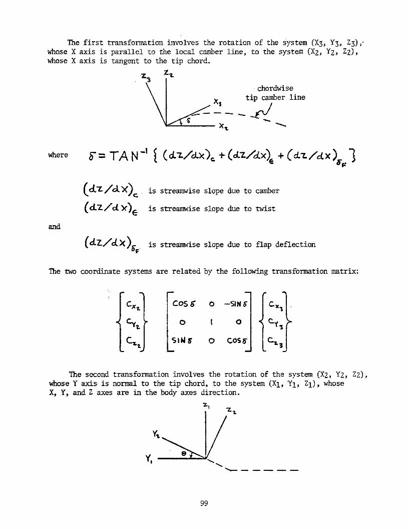
e first transfornation involves the rotation of the system (X3t Y3r Z3)9* whose X axis is parallel to the local camber line, to the system (Xz, Yz, Zz) whose X axis is tangent

chordwi s e tip camber line

- \

-.r 2-J

(~z/Ax)

(dz/& x ) ~ is streamwise slope due to camber

is streamwise slope due to twist

C

and

(dz/dX)& , is streamwise slope due to flap deflection F

The two coordinate systems are related by the following transformation matrix:

The second transformation involves the rotation of the system (Xz, Yz, ZZ) , whose Y axis is normal to the tip chord, to the system (Xi, Y1, Zi), whose X, Y, and Z axes are in the body axes direction.

\

99

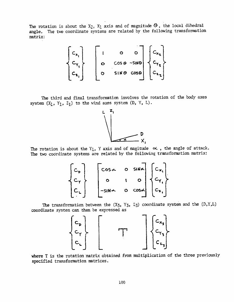
rotation is about the X z 9 X i axis and of magnitude 5 the local dihedral angle. matrix:

The two coordinate systems are related by the following transformation

The third and final transformation involves the rotation of the body axes system (Xi, Y1, Z l ) t o the wind axes system (D, Y, L) .

L =t

The rotation is about the Yl, Y a x i s and of magitude The two coordinate systems are related by the following transformation matrix:

, the angle of attack.

The transformation between the (X3, Y3, Z3) coordinate system and the (D,Y,L) coordinate system can then be expressed as

T

where T is the rotation matrix obtained from multiplication of the three previously specified transformation matrices.

100

ressing Cxg9 Cyg and Czg in terms of the side edge suction parametors, *

we can now write the change in drag, side force and l i f t resulting from the force rotation a t each side edge station:

where

The minus sign on the first term of each equation is for the right side of the configuration and the positive sign is for the l e f t side. are numerically integrated along each t i p chord t o obtain the t o t a l change in l i f t , side force and drag due to side edge force roation.

These force increments

101

APPENDIX C

HYPERSONIC F I N I T E ELEIEN'" ANALYSIS

High Mach number analysis has a number of optional methods for calculating the pressure coefficient. In each method the only geometric parameter required is the element impact angle, 6, or the change in the angle of an element from a previous point.

The methods to be used in calculating the pressure in impact (6 > 0) and shadow (6 < 0) regions may be specified independently. options is presented below.

A summary of the program pressure

Impact Flow Shadow Flow

1. Modified Newtonian 2. Modified Newtonian+Prandtl-Meyer 2. Modified NewtonianfPrandtl-Meyer 3 . Tangent wedge 3 . Prandtl-Meyer f rom f ree-s t ream 4. Tangent-wedge empirical 4. OSU blunt body empirical 5. Tangent-cone empirical 5. Van Dyke Unified 6. OSU blunt body empirical 6. High Mach base pressure 7. Van Dyke Unified 7 . Shock-expansion 8. Blunt-body shear force 8. Input p re s su re coefficient 9. Shock-expansion 9. F ree molecular flow

1. Newtonian (Cp = 0)

10. F ree molecular flow 11. Input pressure coefficient 12. Hankey flat - surface empirical 13. Delta wing empfrical 14. Dahlem-Buck empirical 15. Blast wave 16. Modified tangent-cone

A brief review of these methods will be presented in the following text.

MODIFIEO NEWTONIAN

This method is probably the most widely used of all the hypersonic force analysis techniques. The major reason for this is i t s simplicity. Like all the force calculation msthods, however, i t s validity in any particular application depends upon the flight condition and the shape of the vehicle o r component being considered. Its most general ap- plication is for blunt shapes at high hypersonic speed. form of the mcdified Newtonian pressure Coefficient is

The usual

102

In t rue Newtonian flow ( M = a, Y = 1) the parameter K is taken a s 2 . In the various f o r m s of modified Newtoniar, theory-, K is given values other than 2 depending o n the type o i m2dified Newtonian theory used. K is frequently taken as being equal to the stagnation pressure co- efficient. ship (Reference 19 ) .

In other fo rms it is determined by the following relation-

where

the exact va! - - c- e of the press r e pno s e coefficient at the nose or leading

edge

impact angle at the nose o r leadicg edge

- i - nose

In other work K is determined purely on an empir ical basis.

fn (M, u, shape) - K -

When modified Newtonian theory is used, the p re s su re coefficient in shadow regions (6 is negative) is usually se t equal to zero.

MOQIFIED NEWTONIAN PLUS PRANDTL-EYER

This mzthod, described as the blunt body Newtonian f Prandtl-Meyer technique, is based on the analysis presented by Kaufman in Reference 20. detached shock, followed by an expansion around the body to supersonic conditions. This rn-tthod uses a combination of modified Newtonian and Prandtl-Meyer expansion theory. along the body until a point is reached where both the pressure and the pressure gradients match those that would be calculated by a continuing Prandtl- Meyer expansion.

The flow model used in this method assumas a blunt body with a

Modified Newtonian theory is used

The calculation procedure derived for determining the pressure co- efficient using the blunt body Newtonian -f- Prandtl-Meyer technique is outlined below.

1. Calculate f ree-stream static to stagnation pres sure ratio

2. Assumz a starring value of the matching Mach number, M (for Y = 1.4 asscme iv l = 1.35) 9

9

103

3.

4.

5 .

6 .

7.

8 .

9 .

Calculate mstching point to free-stream stat ic pressure ratio

Calculate new free-stream stat ic to stagnation pressure ratio

1 Y 2 M 4 Q - - 4 p C

Assume a new matching point Mach number ( 1 . 7 5 ) and repeat the above steps to obtain a second set of data.

With the above two t r i e s use a linear interpolation equation to estimate a new matching point Mach number. This process is repeated until the solution converges.

Calculate the surface slope at the matching point

2 - - Q - P 1 - P s in 6

9

Use the Prandtl-Meyer expansion equations to find the Mach number on the surface element, M 6

Calculate the surface pressure ratio

Y

where

is provided a s an empir ical correction factor

is the pressure on the clew-ent of interest

%

p6 10. Calculate the surface to free-stream pressure ratio

104

11 e Calculate the surface pressure coefficient

The resul ts of typical calculations using the above procedure Ere shown in Figure 1, sure coefficient at a zero impact angle. A s pointed out in several references these resul ts correlate well with tes t data for blunl: . shapes. However, i f the surface curvature changes gradually to zero slope some distance f rom the blunt stagnation point the pres - sure calculated by this msthod will be too high. This is caxsed by characterist ics near the nose intersecting the curved shock system and being reflected back onto the body. If the zero slope is reached near the nose (such as in a hemisphere o r a cylinder) this effect has not had time to occur.

Nota that the calculations give a positive pres -

TANGENT-WEDGE

The tangent-wedge and tangent-cone theories a r e frequently used to calculate the p re s su res on two-dimensional bodies and bodies of revolution, respectively. These methods a r e really empir ical in nature since they have no iirm theoretical basis. They are suggested, however, by the resul ts of m3re exact theories that show that the pressure on a surface in impact flow is pr imari ly a function of the local impact angle. calculated using the oblique shock relationships of NACA TR- 11 35 (Reference 21),

In this program the tangent-wedge p res su res are

The basic equation used is the cubic given by

(sin2 0 S )' + b o r

R3

where

e

6

S

b

C

d

f b R 2 t c R t d = o .

shock angle - -

- - wedge angle

w2 t 2 2 -- - Y s in 6 - - ML

2 . sin 6 - 2 M 2 t 1 4

- M4

105

1

C?

20 i o 1 20 lio

Figure 1. Blunt Body Newtonian f Prandtl-Meyer Pressure Results

106

The r o d s of the above cuSic equation may be obtained by using the trigonometric solution procedure {see Reference 22) as ir-dicated below *

Y1 - - 2 i/-BT5- COS (w/3) - b / 3

- - 2 cos (w/3 f 60") - b/3 y2 -

where

roots of the reduced cubic equation - - Y i

3 b c + d 3 2(b/3) - - - - 9

2 - - sin 8, = roots of the cubic equation Ri

The smallest of the three roots corresponds to a decrease i n entropy and is disregarded. never appears in physical actuality.

The iargesr: root is also disregarded since it

10 7

For small deflections, the cubic solution becomes very sensitive to numerical accuracy; that i s , to the number of significant digits c a r - ried. an alternate procedure is used.

Since this is dependent on the particular machine em-plci;ed,

When the flow deflection angle is equal to o r less than 2.0 degrees , the following equation is used inste2d of the above cubic relationships (Reference 23)':

Once the shock angle is obtained the remaining flow properties may be found f r o m the relationships of Reference 21.

density =

- - te mpe r atur e

p re s su re - coefficient -

p2

T2

G p

c T

J 7(M 2 2 sin 8, - 1) (M 2 2 s in O s f 5 )

2 2 36 M sin os

PM2 7 es - I1

0.7 M L

where

)2 = conditions behind the shock

Oblique shock detachment conditions a r e reached when no solution m a y be found to the above cubic relationships. Under these conditions the program uses the Newtonian f Przndtl-Meyer mzthod f o r continued calculations.

108

TANGENT-’WEDGE, TANGENI’-CONE, AND DELTA WING NEWONIAN EMPIRICAL METHOD

The tangent-cone and the tangent-wedge Newtonian empirical methods used in this program a r e based on the empirical relationships derived below.

F o r wedge flow

sin 6

(1 - E) cos (es - “w) s in e,=

For cone flow (thin shock layer assumption)

s in 6 -

Y - 1 Y t 1 S

and cos (e - 6) = 1 = - In the limit as M-a, E = E li m

-- Therefore

wedge

sines = + 2 sini jw

cone

Y + 3

109

These limiting expressions for @ may now be compared with the dzta of TR-1135 (Reference 21) at Y = 7/5 using the following similari ty parameters . The exact equations contaii.1 three va r i - ables - es, 6, and E (. Noting that for 't = constant, E = fn(Mn,j only, the preceding equations may be rewritten in the following form:

wedge cone

L

The parameter (8 - 6) is approximately constant and independent of M except near the shock detachment condition. The equations e s - sentially contain only two variables, M and M sin 6. These are used a s coordinates to plot the data forniedge flow shown in Figure 2, it is seen that the data a r e nearly normalized with the use of these coordinates .

A similar plot could be obtained for cone flow. F r o m the figure

For rapid calcuiations we need relationships fo r Mns as a function of M sin d that satisfy the following requirements:

1. The effect of shock detachment is neglected

2.

3.

At M sin6 = 0, Mns = 1

The sOlution asymptotically approaches the M = a 3 line

at M s in6 = 0 Have the cor rec t slope, d M s i n 6 ns d M 4.

These conditions lead to equations of the following fo rm K -- M' c) L wedge Mns = Kw M' t e

Y t 1 - - Kw - 2

-Kc M' cone M = Kc M ' f e n s

where

M' = M s i n 6

= 2 (Y f 1 ) / ( Y t 3) KC

110

. . . . . ... - . .

. . . . . . -.. .. .. .^. . . ~

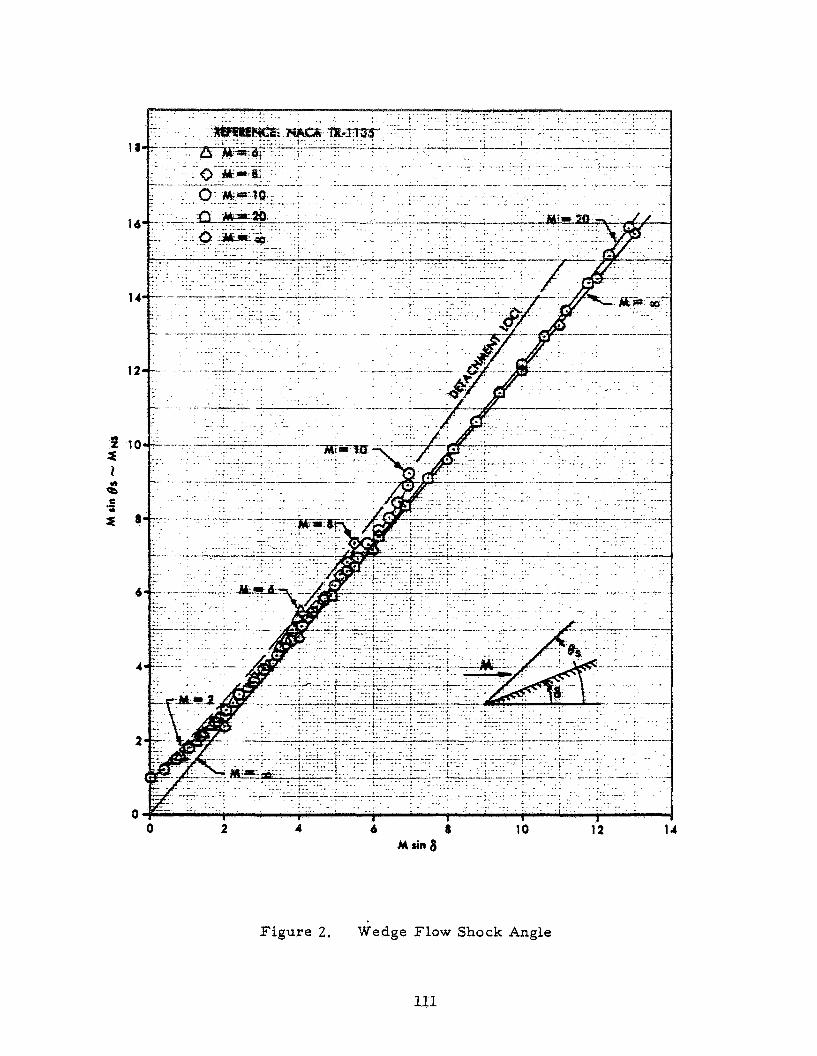
0 2 4 6 8 10 12 M sin 8

Figure 2. Wedge Flow Shock Angle

111

These expressions a r e compared with the data of TR-1135 in Figfires 3 and 4 ~ The c3ne data a r e also shown in Figure 5 with the same scales as in Figure 2 . The pressure coefficient may now be obtained by the following relationships for a wedge and cone respectively.

'2 = 2 sin 6 cP

- 1 ( Y - 1) AXS2 f 2 1 - 4 (Y+ 1) Mns2 ]

Experimental results have shown the pressure on the centerline of a delta wing to be in agreement with two-dimensional theory at small values of the similari ty parameter (MI < 3.0) and with conical flow theory a t higher values, The previous expressions derived for wedge and cone flows have been combined to give these features. given bel ow.

The resulting relationships a r e

For Y = 715

M*s 1.09 M s i n 6 f -0.49 M s in6 e

The similari ty parameter relationship for pressure i s

The shock angle and p r e s s u r e coefficient calculated f rom the above equations a r e coinpared with the experimental resul ts (Refercnce 2 8 ) in Figures 6 and 7 , respectively.

112

. . - . . . . . ... . . . . . .

0 0.4 0.8 t .2 1.6 2.0 2.4 2.8 M sin 8 - M’

Figure 3. Wedge Flow Shock Angle Empirical Correlation

11 3

3.6

3.2

2.8

2.4

e 2.0 z 2 b: e

s .- * 8 1 . A

1 .i

0.1

0.4

0

0 M,=10 (TR-1135)

-K, M ' 0 Masin $5 K,M'+ e a K c EE 1.09

K, =i.136

I 1 I I I 1

0.4 0.8 I .2 1.6 2.0 2.4 M,Sin 8 - M '

8

Figure 4. Conical Flow Shock Angle Empirical Correlatior,

114

18

16

14

12

Q 10 z 2 v) 0 E

0 2 4 6 8 10 12 14 M,Sin 8 - M'

..-

Figure 5 . Conical Flow Shock Angle Empirical Correlation

11 5

4 r 3 c .5 r

0 0 1 2 3 4 5 6

MSina-M'

Figure 6 . Delta W4ng Centerline Shock Angle Correlation

116

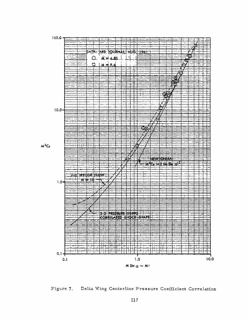
100.0

I

I I

M

1 0.0

1 .a

0.1

0.1 1 .o M 5 i n ~ ! - M l

10.0

Figure 7 . Del t a Wing Centerline F r e s s u r e Coefficient Correlation

11 7

OSU BLUNT BODY EMPIRICAL MF,TJAOD

The OSU (Ohio State University) blunt body empir ical equation describes the pressure distribution about cylinders in supersonic flow. The equation was presented in Reference 25) and was stated to match "all the data obtained on the cylinders in the present tes t se r ies with a maximum deviation of 2.5 percent. " The expression used is

P1

pt 00 - = 0.32 f 0.455 COS 9 t 0.195 COS 2 0 f 0.035 COS 3 9 .. 0.005 COS 4 8

where

9 - - peripheral angle on a cylinder (= 0 at the stagnation point) = 90" - 6

surface pressure

tctal p ressure r i s e through normal shock

- - P1

- - 'trn

The pressure coefficient is calculated f rom the relationship

where

y 2 Pt

Pm - - K j - M t 1

stagnation p res sure coefficient = C - K - Pstag

- f r e e stream pres sure pa Y - - ratio of specific heats = 1.4

Y&V DYKE UNIFIED METHOD

This force calculation mcthod is based on the unified supersonic- hypersonic smal l disturbance theory proposed by Van Dyke in Reference 26 as applied to basic hypersonic similari ty resul ts . The mathod is useful f o r thin profiie shapes and as the name implies extends down to the supersonic speed region.

118

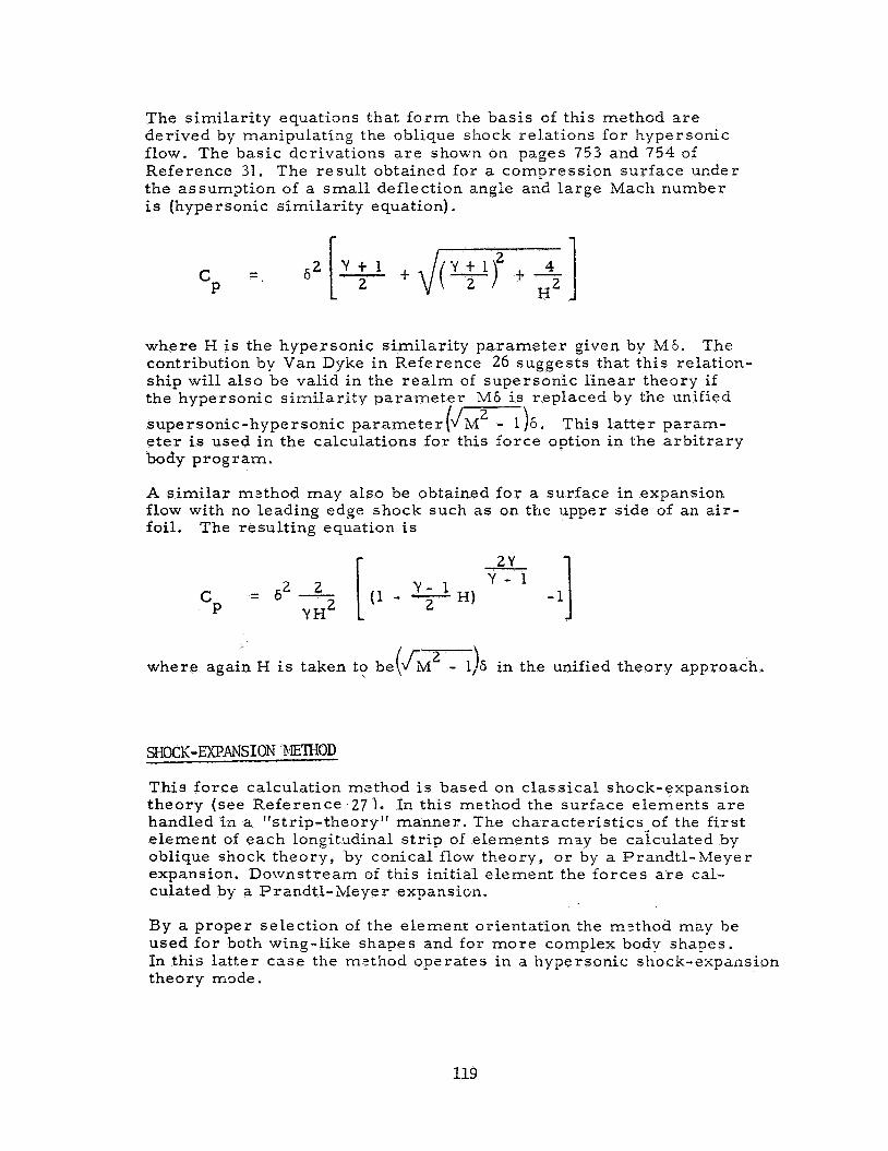
The similari ty equations that fo rm the basis of this method a re derived by manipulating the oblique shock relations for hypersonic flow. The basic derivations a r e shown on pages 753 and 754 of Reference 31. The result obtained for a compression surface ucder the assumption of a small deflection angle and large Mach number is (hypersonic similari ty equation).

where H is the hypersonic similari ty parameter given Sy Md. contribution by Van Dyke in Reference 26 suggests that this relation- ship will a lso be valid in the r ea lm of supersonic l inear theory i f the hypersonic Similarity parameter hf6 is replaced by the unified

supersonic-hypersonic parameter (=)6. This la t ter param- e t e r is used in the calculations for this force option in the arb i t ra ry body program.

A similar mzthod may also be obtained for a surface in expansion flow with no leading edge shock such a s on the upper side of an a i r - foil. The resulting equation is

The

cP - - 6 2 2

Y H2 I -1

2) where again H is taken t? be(LV - 1,6 in the unified theory approach.

SHOCK-EXPANSION NETHOD

This force calculation mcthod i s based on classical shock-expansion theory (see Reference 27 \. In this method the surface elements a r e handled in a “strip-theory” manner. The character is t ics of the first element of each longitudinal s t r ip of elements may be ca’iculated by oblique shock theory, by conical flow theory, o r by a Prandtl-hfeyer expansion. Downstream of this initial element the forces a r e cal- culated by a Prandt l - Meyer expansifin.

By a proper selection of the element orientation the m:thod may be used for both wing-like shapes and for more complex body shapes. In this latter case the m?thod operates in a hypersonic shock-expansion theory mode.

119

F R E MOLECULAR FLOW bETHOD

At very high altitudes conventional continuum flow theories fail and one must begin to consider the general macroscopic mass , force, and energy t ransfer problem at the 5ody surface. This condition occurs when the a i r i s sufficiently rarefied so that the m.?an free path of the molecules i s much grea te r than a characterist ic body dimension. This condition is known as free molecular flow and the method of analysis selected for this program is described in Reference 28. This m.=thod was also used in Refqrence 29. equations used were taken f rom these references and a re presented below.

The

P r e s s u r e coefficient

Shear force coefficient

cf

where

S

n f

ci

Tb

T, e r f

(cos 6}ft

\GS

speed ratio = JY/Z M,

normal momentum accommodation coefficient ( = 1. 0 for Newtonian and = 0. for completely diffuse reflection)

impact angle

body temperature, " K

f r ee - s t r eam temperature, "K

e r r o r function erf (x) = X 2

e dx -X 2

taligential inomentum accommDdation coefficient (= 0. for Newtonian flow and 1 . 0 for completely diffuse reflection)

120

The p rpssu re force acts perpendicular to the surface and this direction is readily obtained since the element normai has already been determined in the geometry subrovtines. tangential mined by taking successive vector products as follows.

The shear force acts in the direction of the velocity component on the surface and this direction is deter-

The procedure is i l lustrated in the accornpaning sketch where the in- ciderLt velocity vector is defined as

and t’-e surface normal a s

First, a surface tangent vector (T) is defined by the c ros s product of the normal and velocity vectors :

- T = T X T + T y j + T Z k

where

= Ny vz - N Z vy TX

Ty =

T Z = N X V y - N V

N Z Vx - NX Vz

Y X

Then the direction of the shear force (g) is given by the c ros s product of the surface tangent and normal vectors ;

- - - - S = S i + S y j + S Z k X

where

121

The final components of the shear force in the vehicle axis sys tem a r e given by

SHEARX = (SHEAR) (Sx) / STOTAL

SHEARy = (SHEAR) (Sy) / STOTAL

SHEARZ = (SHEAR) (Sz) / STOTAL

where

SHEAR is the shear force a s calculated by the free molecular flow equations.

STOTAL =

In using the free molecular flow method the above analysis must be car r ied out over the entire surface of the shape including the base, shadow regions, etc. When the free molecular flow method is selected, it is used for both impact and shadow region.

me plane formed by the velocity vector and the surface normal is referred t o as the velocity plane (shaded region in the sketch), since both the incident and surface velocity are in this plane. This definition is correct for two-dimensional flow, however, it is only an approximation t o the shear direction in the general arbitrary-body case.

HANKEY FLAT-SURFACE ENPIRICAL METHOD

This method uses an empir ical correlation for lower surface p re s su res on blunted flat plates. The method, derived in Reference 30, approximates tangent-wedge at low impact angles and approaches Newtonian at high impact

, angles. The p res su re coefficiect is given by

= 1.95 s in26 t 0.21 cos 6 sin 6 cP

122

This is an impact method that has been derived such that tanpent-cone and Newtonian results a r e approximated, respectively, at low and high values of the impact angle. a r e

The empirical relationships presected in Reference 31

1 + (sin 46) 3 / 4 -

3 / 4 (4 cos 6 cos 26) cP - for 6 < 22.5" 514 (sin 6)

2 C = 2.0 sin 6 P fo r 6 5 22.5O

BLAST 'WAVE PRESSURE INCREPENTS

This method uses conventional blast-wave pa rame te r s to calculate the over- p re s su re due to bluntness effects. Force contributions determined by this procedure must be added to the regular inviscid p re s sx re forces ftzngent- wedge, tangent-cone, Newtonian, etc. ) calculated over the same vehicle geometry. rived by Lukasiewicz in Reference 32:

The specific blast wave solutions used in the P r o g r a m were de-

where CD d

is the nose drag coefficient

is the nose diameter o r thickness

Xo i s a coordinate reference point

and the coefficients A, E3 a r e

v- Axis yrnme tr i c

123

MODIFIED TANGEWT-CONE METHOD

This method, originally developed for use on cones with elliptical c ros s - sections, modifies the tangent-cone resul t by an increment representing the deviation from an average p res su re divided by an average Mach nurnber. More specifically, the following equations a r e used (after Jacobs, Rzference 331:

Cptc - cPaxrg

Mavg cP = CPtc -

where is the surface p r e s s u r e coefficient

is the conventional tangent-cone p res sure Coefficient cP

CPtc

Cpavg is the average p res su re coefficient

= Ccpt A / ~ A , A is element a rea

Mavg is the average Mach number, defined for an equivalent cone having p res su re coefficiei-, + cP,vg*

HIM MACH BASE PRESSURES

For a body in high speed'flow i t might be expected that any base regions would experience total vacuum. That is,

1 - cP - - -- M,2

However, the viscosity of real gases causes some p res su re to be felt in base region and experimental data have shown this to be roughly 70% vacuum for air. Therefore, the expression

has been included in the program.

124

Aerodynamic Preliminary Analysis System I1 Part I - Theory

I 7. Author(s1 I 8. Performing Organization Report No.

1 E. Bonner, W. Clever, K. Dunn I NA-80-374 10. Work Unit No.

9. Performing Organization Name and Address Rockwell International Corporation North American Aircraft Division Los Angeles, California 90009

11. Contract or Grant No. Ml-15674

13. Type of Report and Period Covered

12. Sponsoring Agency Name and Address Contractor Report National Aeronautics and Space Administration I Langley Research Center 14. Sponsoring Agency Code

Hampto n. Virginia 23665 I 15. Supplementary Notes

Langley technical monitor: Alan W . Wilhite Part I Final Report

16. Abstract

An aerodynamic analysis program based on potential theory with edge con- siderations at subsonic/supersonic speeds and impact type finite element analysis at hypersonic conditions is described. multiple nm-planar surfaces of arbitrary planform and bodies of non-circular contour may be analyzed. directional characteristics may be generated.

Three dimensional configurations having

Static, rotary, and control longitudinal and lateral-

The analysis has been implemented bn a time sharing system in conjunction with an input tablet digitizer and an interactive graphics input/output display and editing terminal to maximize its responsiveness to the preliminary analysis problem. supersonic speeds and 1 CPU second/kch number/attitude at hypersonic conditions for a typical simulation indicates that program provides an efficient analysis for systematically performing various aerodynamic configuration tradeoff and evaluation studies.

cM= 175 computation time of 45 CPU seconds/Mach number at subsonic-

subsonic Unclassified - Unlimited supersonic hypersonic

N-305 For sale by the National Technical Information Service, Springfield, Virginia 22161