Measurement and Sources of IncomeInequality in Rural and Urban Nigeria

A.S. OyekaleA.I. AdeotiT.O. Oyekale

PMMA Network Session PaperPMMA Network Session PaperPMMA Network Session PaperPMMA Network Session PaperPMMA Network Session Paper

A paper presented during the 5th PEP Research Network General Meeting,June 18-22, 2006, Addis Ababa, Ethiopia.

MEASUREMENT AND SOURCES OF INCOME INEQUALITY IN RURAL AND URBAN NIGERIA

A.S. Oyekale (PhD)*, A.I. Adeoti (PhD)** and T.O. Oyekale*** Department of Agricultural Economics,

University of Ibadan, Ibadan, Nigeria.

*asoyekale@yahoo.com **jadeoti@yahoo.co.uk

***olayemitolulope@yahoo.com Tel: +2348023095901;

+2348029468630

REVISED FINAL REPORT

SUBMITTED TO

POVERTY AND ECONOMIC POLICY NETWORK,

UNIVERSITÉ LAVAL, CANADA.

MAY 2006

2

Abstract

Income inequality and poverty are closely related. This study decomposed

the sources of inequality and poverty in Nigeria. Household survey data

obtained from the National Bureau of Statistics (NBS) were used. Results show

that in 2004, income inequality is higher in rural areas than urban. Employment

income is income inequality increasing while agricultural incomes decreases

inequality. Inequality between the states, rural-urban areas, and geopolitical

zones accounted for the greater portion of observed inequality. Urbanization,

residence in the southwest zone, household size, house head’s formal education,

number of time suffered from illness, engagement in paid job, involvement in

non-farm business, formal credit and informal credit increased income

inequality. Between 1998 and 2004, income redistribution and income growth

increased poverty. It was recommended, that welfare enhancing programs that

will benefit urban/rural poor should be identified, while better economic

opportunities should be created for those in rural areas.

Keywords: Income inequality, poverty, decomposition, economic opportunities,

Nigeria

JEL classification: D3, O15, O55

3

Introduction

The pattern of income distribution has been a concern to economists for a

long time (Clarke et al, 2003). Specifically, the 1990s witnessed resurgence in

theoretical and empirical attention by development economists to the

distribution of income and wealth (Atkinson and Bourguignon, 2000). This is

because high level of income inequality produces an unfavorable environment

for economic growth and development. In many developing countries, studies

have shown that income inequality had risen over the last two decades (Addison

and Cornia, 2001; Cornia with Kiiski, 2001; Kanbur and Lustig, 1999). Despite

commitments shown by many developing countries towards reducing income

inequality and poverty, there is lack of sufficient knowledge of how to design a

holistic approach for addressing the issues (Matlon, 1979). The widening

dimension of poverty has now aroused serious humanitarian concerns and fears

of political instability. It has become evident that in absence of strong foreign

markets, the domestic inter-sectoral linkages, local infrastructure and policy

environment required for rapid economic growth cannot be provided where

inequality and poverty persist (Aigbokhan, 1999; Clarke et al, 2003).

In Nigeria, accompany the rapid economic growth that was had between

1965 and 1974 was a serious income disparity that is believed to have widened

substantially. Despite past policy interventions to correct this abnormality,

income inequality has increased the dimension of poverty. Aigbokhan (1997,

1999) found that income inequality worsened after the Structural Adjustment

Program (SAP) of 1986. Similarly, poverty incidences were 28.1, 46.3 and 65.6

percent in 1980, 1985 and 1996, respectively (World Bank, 1996; IMF, 2005). Also,

a high level of income inequality exists between Nigeria’s rural and urban areas.

This is because most rural communities depend on agriculture, while urban

engage mostly in paid jobs. However, income inequality results to discontent,

violence and corruption, and as part of microeconomic objectives, governments

always give equitable distribution of income a priority. This is important because

4

income inequality is closely related to poverty (Addison and Cornia, 2001;

Adams, 1999; Adams and He, 1995; Aboyade, 1983), and a careful study of it

gives some insights into the incidence of poverty.

Studies on decomposition of income inequality are desirable for both

arithmetic and analytic reasons (Litchfield, 1999). Policy makers may wish to

understand the link between the socio-economic characteristics and total income

inequality. This sheds light on the structure and dynamics of income within

different socio-economic groups in the economy. Estimating the contribution of

each income source to total inequality is very helpful. This information helps to

understand the effect that changes in household labor force participation can

make on income distribution (Fournier, 1999). Recent advances towards

understanding of the linkage between poverty and income inequality make it

possible to determine the contributions of income redistribution and income

growth to poverty change within a period of time. This information is very

helpful to economic policy analysts and designers of poverty reduction

programs.

This study intends to fulfill four objectives. First is to provide a descriptive

analysis of households’ income from different sources and determine the level of

income inequality. Second is to estimate the contributions of the income sources

to overall income inequality and find the within-between contributions. Third is

to determine the contributions of some households’ socio-economic

characteristics to income inequality. Fourth is to analyze the contributions of

income growth and income redistribution to poverty change. Objectives one, two

and four were extensively analyzed with the DAD 4.4 statistical package by

Duclos et al, (2005). The working hypothesis is that attainment of formal

education does not significantly increase households’ per capita real incomes.

The remaining parts of the paper contain conceptual framework and literature

review, decomposition methods, results and discussions, and policy implications

and conclusion.

5

Conceptual framework and literature review

Inequality implies dispersion of a distribution, whether one is considering

income, consumption or some other welfare indicators or attributes. Although

conceptually distinct, income inequality is often studied as part of the broad

+analyses covering poverty and welfare. However, inequality is a broader

concept than poverty because it is defined over the whole distribution

(Litchfield, 1999; Cowell, 1999). Since Atkinson (1970), most questions about the

measurement of inequality have been formulated using the explicit logic of social

choice theory. In this case, desirable properties are articulated and the indices or

methods are judged according to how well they conform to some selected

properties. There were debates about the merits and demerits of various

subsidiary properties, until reasonable consensus was reached (Morduch and

Sicular, 2002).

Pigou (1912) and Dalton (1920) proposed the Pigou-Dalton transfer

principle. This stated that inequality increases when there is transfer of income

from a poorer to richer person (Atkinson, 1970). Most measures of inequality in

literature (Generalized Entropy, Atkinson, Gini coefficient) satisfy this principle.

Also, Dalton (1920) proposed the population principle of income inequality

measurement, which stated that inequality measures are invariant to replications

of the population. This implies that merging two identical distributions will not

alter the level of inequality. The anonymity principle (symmetry), proposed that

inequality measures are independent of any characteristic of individuals other

than their income (Litchfield, 1999).

The work of Kuznets (1955, 1963) on the relationship that exists between

development and income inequality inspired development economists to find

the major sources of income inequality. The regression analytical approach to

inequality decomposition was pioneered by Oaxaca (1973) and Blinder (1973).

This effort was set to determine the contributions of some socio-economic

variables to income inequality. Fei et al, (1978) also proposed a statistical

6

approach that decomposed income in a way that pinpointed the contributions of

each income source to overall inequality. The perceived linkage between income

inequality and poverty motivated Datt and Ravallion (1992) to propose a method

that decomposed poverty change into the income redistribution, income growth,

and a residual components, otherwise known as the black box. Kakwani (1997)

used axiomatic approach to decompose poverty change into their growth and

redistribution components. This was confirmed by the Shorrocks (1999) method

that applied the Shapley (1953) theory to poverty decomposition. This was able

to take care of the problematic residual component that was left in the Datt and

Ravallion (1992) method.

The relevance of income inequality to economic development efforts can

be judged by the spread of researchers that have kept close focus at it since the

past few decades. In Nigeria, Adelman and Morris (1971) estimated a Gini

coefficient of 0.51. Aboyade (1974) used the 1966/67 household data and

estimated a Gini coefficient of 0.58. Etukodo (1978) found that income inequality

was higher in urban Lagos than a rural area in Cross Rivers State. In 1996/97,

Gini index for Nigeria was 0.506, while it was 0.613 in 1998 (World Bank, 2003).

Matlon (1979) found that non-farm income had negative impact on the

distribution of rural income in Nigeria because it was mainly concentrated

among large landowners. In Zimbabwe, Piesse et al (1998) used Gini

decomposition and found that non-farm income decreased income inequality in

Chiweshe. In rural Egypt, Adams (1999) analyzed the impact of non-farm income

on income inequality. Results showed that although non-farm income

represented the most important inequality-decreasing source of income,

agricultural income represented the most important inequality-increasing source

of income. Ssewanyana et al (2004) found that in Uganda, non-farm income was

inequality increasing, although not all sources of non-farm income have

unfavorable effect on income distribution among the rural population.

7

Fields and Yoo (2000) proposed a regression-based method for analyzing

the contributions of socio-economic characteristics to change in labor income in

Korea. It was found that between 1986 and 1993, the job tenure, gender, years of

education and occupation explained the level of income inequality, while

education, industry, occupation and potential experience accounted for change

in income inequality. Morduch and Sicular (2002) also proposed a regression-

based approach for decomposing income inequality. The approach provided an

efficient and flexible way to quantify the roles of variables like education, age,

infrastructure, and social status in a multivariate context. Using data from China,

the results illustrated the sharp differences that can result when using

decomposition methods with varying properties.

Alayande (2003) decomposed income inequality in Nigeria with the

Morduch and Sicular (2002) method. With 1996/1997 data, the Gini

decomposition method revealed that primary and post-secondary educational

attainments are important in reducing income inequality, while the number of

unemployed persons in the households contributed positively to income

inequality. Wan and Zhou (2005) applied regression-based approach using a

combined Box-Cox and Box-Tidwell income generating function to decompose

income inequality in rural China. Results showed that capital input and farming

structure were the most significant factors explaining income inequality.

Baye (2005) used the Shapley Value for assigning entitlements in

distributive analysis and assessed the within- and between-sector contributions

to changes in poverty levels in Cameroon between 1984 and 1996. It was found

that the within sector effects disproportionately accounted for increase in

poverty, but the between-sector contributions in both rural and semi-urban areas

increased poverty. Araar (2006) used the Shapley value to decompose Gini

coefficient and generalize it to other inequality indices. It was concluded that, if

well interpreted, the analytical approach can give convincing results on the

contribution of each component factor. Using data from Cameroon, it was found

8

that rural areas contribute less than the urban areas to total inequality while

about two-third of the total inequality was explained by the nonfood in the

expenditure components decomposition.

Kakwani (1990) explored the relation between economic growth and

poverty, and developed the methodology to measure separately the impact of

changes in average income and income inequality on poverty. This

decomposition provides a link between macro-economic adjustment policies and

poverty, which is discussed in the context of the adjustment experience of Cote

d'Ivoire. Son (2003) proposed a poverty decomposition approach that can be

used to analyze changes in poverty over time into such components as the

overall growth effect while assuming that inequality in the distribution does not

change, the impact of differences in growth rates between the groups, the effect

of the change in inequality within the different groups and the impact of changes

in the population shares of the various groups.

Ravallion and Chen (2003) introduced the growth incidence curve (GIC) to

measure the rate of growth over the relevant time period at each percentile of the

distribution (ranked by income or consumption per person). Their rate of pro-

poor growth is the mean growth rate of the poor, which gives the change in the

Watts index per unit time divided by the headcount index. Ravallion (2004)

submitted that the measure of the rate of pro-poor growth proposed by Ravallion

and Chen (2003) is the ordinary rate of growth times a “distributional correction”

given by the ratio of the actual change in poverty over time to the change that

would have been observed under distribution neutrality. If growth is pro-poor,

the rate of pro-poor growth will exceed the ordinary rate of growth. If the

distributional shifts go against the poor, then it is lower than the ordinary rate of

growth.

Son (2004) also proposed a ‘poverty growth curve’ that measures whether

economic growth is pro-poor or not pro-poor. The methodology was developed

9

based on Atkinson's theorem linking the generalized Lorenz curve and changes

in poverty. The approach seemed to give satisfactory results in some statistical

investigation and testing with data from Thailand and some other cross-

countries data. Duclos and Wodon (2004) also proposed simple graphical

methods to test whether distributional changes are pro-poor or not. Based on

definition of some terminologies, it was noted that issue of whether pro-poor

growth should be absolute or relative is of paramount importance and whether

more emphasis should be placed on the impact of growth on the poorest

population.

Kalwij1 and Verschoor (2005) analyzed the impact of globalization on

poverty by quantifying explicitly the responsiveness of poverty to aggregate

changes in income in six developing regions between the period 1980-98 using

the Shapley method. It was found that differential income growth accounts for

most of the diversity in poverty trends, both across regions and over time, but

leaves a substantial amount of variation unexplained. The impact of changes on

inequality is relatively small, except in Eastern Europe and Central Asia.

Data and Analytical Approaches

The Data

The data used were collected by the Nigeria’s National Bureau of Statistics

(NBS) {formerly known as the Federal Office of Statistics (FOS)}. They were

based on National Living Standard Survey (NLSS) of households that was

carried out between September 2003 and August 2004. The sample design was

two-stage stratified sampling. At the first stage, from each State and the Federal

Capital Territory (FCT, Abuja), clusters of 120 housing units called Enumeration

Area (EA) were randomly selected. The second stage involved random selection

of 5 housing units from the selected EAs. A total of 600 households were

randomly chosen in each of the States and the FCT, summing up to 22,200

households in all (FOS, 2003). However, some households did not fully complete

10

the questionnaires. Out of the 22,200 households that were targeted, only 19,158

completed the survey. However, because many did not record their incomes,

data for this study comprised of 15141 households from the 36 States and the

FCT. These are those whose income sources were fully provided in the data set.

Data set from the Household Expenditure Survey of 1998 were also used in order

to fulfill the fourth objective. This data comprises of 18977 households.

The concept of income used in the study reckons with income earned both

in cash and in kind. Therefore, money values were allocated to receipts of income

in kind and household consumption of crops and livestock produced based on

prevailing market prices. It was possible to compute profits from farming

because the data included issues related to cost of production. Recognition was

made of whether incomes recorded were incomes before or after taxation. This

study identified the following (9) sources of income: employment (wage income),

agricultural income, non-farm businesses, remittances/grants, credits (formal),

asset disposal/rental, informal borrowing, government transfers and informal

transfers (etc. begging).

Measurement of income inequality

In order to achieve the first objective, descriptive statistics like mean,

percentage, standard deviation and variability index (mean/standard deviation)

were used. In order to calculate Gini coefficient, Morduch and Sicular (2002)

noted that where incomes are ordered so that Y1 ≤ Y2 ≤ Y3 ≤…… ≤Yn, the Gini-

coefficient can be computed as: n

Gini i i i 2i 1

2 n 1I (Y) a (Y)Y and a (Y) i2n=

+⎛ ⎞= = −⎜ ⎟µ ⎝ ⎠∑

……. 01

Where n is the number of observation, µ is the mean of the distribution, Yi is the

income of ith household and i is the corresponding rank of income. This measure

of income inequality conforms with the Pigou-Dalton transfer principle, income

scale independence, principle of population, and anonymity or symmetry but

11

fails the decomposability axiom if the sub-vectors of income overlap. However,

several authors have shown that Gini-coefficient can be decomposed successfully

(Litchfield, 1999).

Decomposition based on Gini-coefficient

Decomposition of Gini index was originally developed by Rao (1969).

Following Pyatt et al (1980), Gini-coefficient can be decomposed given that:

iG

Cov(Y ,i)I (Y)n

=µ 02

The variables are defined in equation 1 and Cov is covariance.

The Gini coefficient of the ith source of income, IG(Ys) can be expressed as

sG s

s

Cov(Y ,i)I (Y )n

=µ 03

Since total income is the sum of source incomes, the covariance between the total

income and its rank can be written as the sum of covariances between each

source income and rank of total income. The total income Gini can then be

expressed as a function of the source Ginis.

s

G s G ssI (Y) R I (Y )µ=

µ∑ 04

Where Rs is the correlation ratio expressed as:

( )( )s

s

Cov Y,iR

Cov Y ,i=

05

Similarly, s ss w g 1=∑ 06

ssw µ=µ 07

G ss s

G

I (Y )g RI (Y)

= 08

where wsgs is the factor income inequality weight of the an income source in

overall income inequality or the the relative contribution of source s, ws is the

12

source income weight or the income share of source s and gs is the relative

concentration coefficient of the sth source in overall inequality. An income source

increases overall income inequality when gs >1 and it decreases it when it is <1.

The Within-Between (Intra-Inter) Inequality Decomposition

In order to achieve part of the second objective, the within-between group

contributions to income inequality was decomposed. Litchfield (1999) submitted

that given a member of Generalized Entropy class of income inequality

represented as:

ni

GE GE2i 1

Y1 1I (Y, ) 1 0 In

α

=

⎡ ⎤⎛ ⎞⎢ ⎥α = − ≤ ≤ ∞⎜ ⎟µα −α ⎢ ⎥⎝ ⎠⎣ ⎦∑

9

α represents any real value capturing the weight given to the distance between

incomes at different parts of the income distribution. Lower α is sensitive to

lower tail of the distribution, while higher α is sensitive to changes in the upper

tail. During estimation, α can be specified as 0, 1 or 2. When α is 0, more weight

is given to the distances between incomes in the lower tail, α equals gives equal

weight across the distribution while α equal 2 gives proportionately more

weight to gaps in the upper tail. In this study, α was specified as 2. When GE(α )

= 0, there is perfect equality in distribution. The within (intra) group inequality

can be expressed as: S

GE,WITHIN s GE Ss 1

I I (Y , )=

= λ α∑ 10

ααλ −= 1f sss v 11

Where fs is the population share, and vs is the income share of each partitions s,

j=1,2,3….h. Similarly, the between (inter) group inequality can be expressed as:

S

GE,BETWEEN s s2s 1

1I f w 1α

=

⎛ ⎞= −⎜ ⎟α −α ⎝ ⎠

∑ 12

Cowell and Jenkins (1995) have shown that Ib +Iw =I total

13

Regression-based decomposition

For the third objective, the regression based decomposition approach

proposed by Morduch and Sicular (2002) was used. The per capita real income

and per capita adult equivalent income were the measures of welfare, which

served for decomposing the sources of income inequality. The decomposition is

done by specifying an income function as:

Y=Xβ + ε 13

Given that β is an M-vector of regression coefficients, Y is the per capita

real income (N) and X is an n x M matrix of independent variables. The socio-

economic variables included in the regression are contained in table 1 and ε is the

stochastic error term.

Following the conventional decomposition approach, ∑=

=s

ssi YY

1

the

contributions of each of the socio-economic factors (Xi) to Gini income inequality

is decomposed as:

nm m

im i 1

n

ii 1

n 1 ˆi X2

s(X , Y)n 1i Y

2

=

=

⎛ ⎞+⎛ ⎞− β⎜ ⎟⎜ ⎟⎝ ⎠⎜ ⎟=

⎜ ⎟+⎛ ⎞−⎜ ⎟⎜ ⎟⎝ ⎠⎝ ⎠

∑

∑ 14

This inequality decomposition can be applied to several inequality indices like

Theil-T, Theil L and coefficient of variation (CV). However, Morduch and Sicular

(2002) found that parameters estimated in the different approaches had different

signs. It was therefore noted that for proper policy making, a choice must be

made between these methods. In this study, we used the CV approach. This was

computed as:

m m m mi im m i

CV VARi ii

ˆ ˆ(Y ) X Cov( X , Y)s (X , Y) s (X , Y)Var(Y)(Y )Y

⎡ ⎤−µ β ⎡ ⎤β⎢ ⎥= = = ⎢ ⎥

−µ⎢ ⎥ ⎣ ⎦⎣ ⎦

∑∑ 15

14

The Datt and Ravallion approach to poverty decomposition

For the fourth objective, the decomposition approach proposed by Datt

and Ravallion (1992) was used to decompose observed change in poverty into

growth, redistribution and the residual components. The growth effect measures

changes in poverty that will be obtained when Lorenz curves does not change

Redistribution effect evaluates the effect of shift in Lorenz curve, while residual

looks at the effect of interaction between growth and redistribution. The

decomposition follows by identifying a reference period, k, the variation in

poverty between poverty between 2 periods (t and t+n) given a poverty line (z)

and Lorenz curve (L) can be decomposed as:

434214342143421sidualInequalityGrowth

tt kntkRknttdknttGPPRe

1 ),,(),,(,,( +++++=−+ 16

Where

⎟⎟⎠

⎞⎜⎜⎝

⎛−⎟⎟

⎠

⎞⎜⎜⎝

⎛=+

+k

tk

nt

LzPLzPknttG ,,),,(µµ

17

⎟⎟⎠

⎞⎜⎜⎝

⎛−⎟⎟

⎠

⎞⎜⎜⎝

⎛=+ + t

knt

k

LzPLzPknttD ,,),,(µµ

18

R(t,t+n,t) = G(t,t+n,t+n) – G(t,t+n,t) = D(t,t+n,t+n) + D(t,t+n,t)

19

The Shapley Approach to poverty decomposition

The Shapley decomposition method proposed by Shorrocks (1999) from

the concept introduced by Shapley (1953) was also used for the fourth objective

(see Shorrocks, 1999 for some details). The proposed framework is for

decomposition analysis, whether static or dynamic and whether it concerns

poverty or inequality in the distribution of living standards. It also has the

advantage of eliminating the “black box” that remained unexplained in many

conventional decomposition techniques. Given a fixed poverty line z, the poverty

level at time t may be expressed as a function P(µt, Lt) of mean income µt and the

15

Lorenz curve Lt. The growth factor in the change in poverty between period t

and t+n is denoted by 1t n

t

G µµ+= − and the redistribution factor by t n tD L L+= − .

The exercise becomes one of identifying the contribution of growth, G, and

redistribution, D, in the decomposition of changes in any poverty measure that is

additively decomposable. The Pα class of poverty measures (Foster et al., 1984)

was used and it addresses poverty incidence (α = 0), poverty depth (α = 1) and

poverty severity (α = 2). The aggregate change in the Pα class of poverty

measures is given as:

),,,(),,( zLPzLPP ttntnt µµ −=∆ ++ 20

This is an expression of the change in poverty, Pα∆ which was decomposed into

the growth (G) and redistribution (D) components are given as:

),,(),,( zLPzLPG tttnt µµ −= + 21

),,(),,( 1 zLPzLPD ttntnt +++ −= µµ 22

According to Kolenikov and Shorrocks (2003), equation 21 indicates the marginal

effect of the change in mean income with distribution held constant while

equation 22 computes the marginal impact of redistribution when mean income

is held constant. This two effects should be averaged and further expressed as:

)],,(),,([21)],,(),,([

21 zLPzLPzLPzLPG ttntnttttnt µµµµ −+−= +++ 23

)],,(),,([21),,(),,([

21 zLPzLPzLPzLPD ntntntntttntt +++++ −−−= µµµµ 24

Results and Discussions

Description of Data

Table 1 shows the descriptive statistics of some variables in the data set.

The arithmetic and weighted means were computed for each of the variables.

The total sampling weight is 104,353,742. The male house heads constituted 86.85

percent of the respondents with a weighted mean of 87.68 percent. Average age

16

of the house heads is 47.11 years with weighted mean of 47.59 years. Average

family size is 4.97 with weighted mean of 6.40. Similarly, the adult equivalent

household size is 3.89 with weighted mean of 5.20. Those who were currently

married (monogamy or polygamy) constitute 91.10 percent with weighted mean

of 93.18 percent. Formal education was attained by 62.22 percent of the house

heads, although the highest proportion (18.25) percent had primary leaving

certificate.

The income data were deflated with price index in each of the

enumeration area (see appendix 1). It should be noted that while average

consumer price indices is 1.0539 for the respondents, Rivers State, Delta State,

Bauchi State, Edo States and FCT have the highest values of 1.4592, 1.3796,

1.3628, 1.347 and 1.3603, respectively. Average total annual real income of the

households is N108,848.41 with weighted mean of N150,242.15. Its variability

index is 74.63 percent. The undeflated total income (nominal income) has a mean

of N114,632.72, with weighted mean of N159,864.78. The variability index is

73.82 percent.

The average per capita adult equivalent real income is N 34,909.00 (about

$268.53) with weighted mean of N33,785.84. This translates into average of

N2,903.08 per month. However, average per capita nominal income is N27,472.16

with weighted mean of N27,634.55. Average real income from employment

income is N 34818.00 with weighted mean and variability index of N53,006.87

and 34.13 percent, respectively. Average real agricultural income is N35204.93

with variability index of 58.36 percent. Incomes from non-farm businesses has a

variability index of 39.10 percent.

Gini-inequality indices

Inequality indices of the rural and urban households in different States

and geopolitical zones (GPZ) in Nigeria are presented in tables 2. In the

combined analysis for all the sectors (henceforth CAS), Gini inequality index for

17

the total income is 0.5802, which implies that income inequality is high in

Nigeria. Among the income sources, agricultural income source has the lowest

Gini (0.6987), while incomes realized from government transfers records the

highest inequality (0.9944). Gini inequality index of total income is higher in

rural areas (0.5808) than urban (0.5278). At the GPZ, Gini inequality index for

total income is highest in South East (0.6198), while South West records the

lowest (0.5217). It should be noted that among the income sources, agricultural

incomes from the north east and north west have the lowest Gini indices of

0.6316 and 0.6410, respectively. At the state level, inequality of total income is

lowest in Bauchi, Lagos, Ondo and Ekiti States with 0.4012, 0.4508, 0.4854 and

0.4901, respectively. Also, Adamawa, Taraba, Imo and Bayelsa states have the

highest Gini indices with 0.7021, 0.6519, 0.6268 and 0.6046, respectively. Among

the income sources, agricultural income source has the lowest inequality in many

of the States with Yobe and Gombe States having the lowest Gini indices of

0.5021 and 0.5147, respectively.

Contribution of income sources to overall income inequality

The analyses of the contributions of income sources were done based on

GPZ, sector of the economy (rural and urban) and for the CAS. Table 3 presents

the results for the GPZ. It shows that in North West and North East, agricultural

income accounts for the highest proportion of total income with 47.11 and 41.48

percents, respectively. However, employment income accounts for the highest

proportion of total income in the North Central (34.82 percent), South South

(40.57 percent) and South East (33.37 percent). In South West, income from non-

farm business accounted for the highest proportion of total income with 36.47

percent.

Table 3 further shows that in all the GPZ, employment income is income

inequality increasing. This is because, its share of total income is lower than its

relative contributions to total income inequality. For instance, in North East, it

18

accounts for 35.13 percent of total income and contributes 48.15 percent. It should

be noted that in all the GPZ, agricultural income’s share of total income is less

than its relative contribution to income inequality. This implies that it is income

inequality decreasing. Also, in all the GPZ (except South South), the share of

income realized from non-farm business in total income is lower than its relative

contribution to income inequality. However, the margin is not too wide for zones

like North East, North Central, South West and South East. This implies that

promotion of non-farm businesses has the potentials of boosting the incomes of

the poor and reducing inequality. Government transfer has high coefficient of

concentration, showing it is income inequality increasing in all the GPZ.

Table 4 shows the contribution of the income sources to overall income

inequality in urban areas. It reveals that incomes from paid employment

accounts for the largest share of total income with 41.06 percent and contributes

48.12 percent to total income inequality. Given the importance that public and

private salaried jobs take in Nigerian urban centers, the proportional

contribution of this income source to overall income inequality is not too much.

Incomes from non-farm businesses accounts for 40.28 percent of the total

incomes, but contributes 37.38 percent to total income inequality. Similarly,

agricultural incomes contributes 10.63 percent to total income from urban areas

but accounts for 7.39 percent of the total income inequality. This reveals that

urban agricultural production in the form of livestock husbandry, fisheries, and

crop production may deliver more income in the hands of the urban poor.

Incomes from disposal of assets, informal borrowing and informal transfers also

have the lowest contributions to total urban income, although they are inequality

decreasing.

For the rural areas, the contributions of the income sources to overall

income inequality are presented in table 5. It reveals that employment income

contributes 25.82 percent of the total incomes and accounted for 34.70 percent of

total inequality. Therefore, increasing the incomes from employment increases

19

income inequality in rural areas since the rich among them will further benefit.

Agricultural incomes contributes 47.10 percent of total incomes, but accounts for

36.91 percent of total inequality. This shows that increasing incomes from

agricultural sources will reduce inequality in the rural areas. This is expected

because inducement for increased agricultural production in the rural areas is a

direct effort to raise the incomes of the poor. Incomes from non-farm private

businesses contributes 19.85 percent of the total incomes, but accounts for 21.98

percent of inequality. This shows that major opportunities for non-farm business

in the rural areas are concentrated among the rich although the proportional

contribution to income inequality is not too much. This is expected because the

poor lacks the financial means for participating in profitable business ventures in

the rural areas. Similarly, while incomes from remittances/grants, assets,

informal borrowing and informal transfers contribute 2.04, 1.21, 1.22, 0.60 percent

to total rural income, they accounted for 1.75, 0.97, 1.03 and 0.40 percent,

respectively, of total inequality. All these income sources will reduce income

inequality.

The contributions of the income sources to overall inequality in the CAS

are presented in table 6. It shows that agricultural incomes contributes the

highest proportion of 32.34 percent to total incomes and accounts for 21.70

percent to total inequality. This shows that increasing incomes from agriculture

for the CAS would make more income to be given to the poor and income

inequality will decrease. Income realized through paid employment contributes

31.99 percent of total income and accounts for 40.98 percent of total inequality.

This shows that efforts to increase employment income will not lead to reduction

in income inequality, as more income will be concentrated in the hands of the

rich. Incomes from non-farm business contributes 28.11 percent of total incomes

and accounts for 30.51 percent of total income inequality. This source is

inequality increasing. Also, incomes from remittances/grants, credit (formal),

assets, informal borrowing and informal transfers accounted for 2.44, 1.96, 1.04,

20

1.10, 0.72 percents of total incomes and contributed 2.00, 1.94, 0.80, 0.84 and 0.57

percents of total inequality respectively. These sources are inequality decreasing.

Between and Within Group Inequality Decomposition

Tables 7 shows the decomposition of the computed income source Ginis

into the between and within group inequality components across the Nigeria’s 36

states and the FCT. It shows that inequality between the states accounts for the

greater portion of observed inequality. Specifically, in the total incomes, 97.23

percent of the estimated Gini is accounted for by differences between the

incomes from the states. It should be noted that Oyo, Lagos and Osun have the

largest share of the real total incomes with 5.70, 5.47 and 5.34 percents,

respectively. States with lowest shares are Ebonyi (0.86 percent), Cross Rivers

(0.70 percent) and Benue (0.46 percent) (see appendix 1).

Similarly, table 8 shows the contribution to the inequality components

based on sector of the economy (urban and rural). It shows that inequality

among the income sources from rural areas accounted for the higher proportion

of the Ginis computed for each income source. Specifically, contribution of rural

areas to inequality in total income is 0.2522 (43.46 percent) while the differences

between rural and urban incomes accounted for 0.2702 (46.57 percent). The inter-

and intra-group analysis also shows that differences in incomes within each of

the sectors accounted for greater portion of the computed Ginis for all the income

sources and total income. It should be noted that while rural sector constitutes

72.94 percent of the population share, it accounts for 59.54 percent of total real

income while urban areas accounts for 40.46 percent real total income, although

accounting for 27.06 of the samples (see appendix 1).

Based on differences in GPZ, table 9 presents the results of the between-

within decomposition of the income sources. Between group inequality also

accounts for the highest portion of income Gini coefficient in all the income

sources and total income. It accounts for 82.75 percent, 83.16 percent, 82.15

21

percent and 82.79 percent in total income, employment income, agricultural

income, and non-farm business income, respectively. It further shows that in

many of the income sources, North West and South West zones contributes most

to within income inequality.

Regression Based Decomposition

Tables 10a, 10b and 10c present the results of the regression-based

decomposition using the CV inequality index. In order to remove collinear

variables, the tolerance levels of the variables were computed using the SPSS 10.0

statistical package. The results of the analyses are presented for the CAS (table

10a), urban sector (table 10b) and rural sector (table 10c). The analyses were done

with per capita household income and per capita household adult equivalent

income. The former was computed with the household size, while the latter was

computed with the adult equivalent of each household, as presented in the data

set. However, except where noticeable contradictions are found, interpretations

were made based on per capita household income.

In table 10a, the parameter of urbanization for the CAS reveals that those

from urban centers have significantly higher per capita income (p<0.01). This is

expected because averagely, Nigeria’s urban centers offer more opportunities for

income generation than rural areas. DFID (2004) submitted that poverty is higher

in rural Nigeria than the urban and per capita incomes in urban areas are

roughly a third higher than in rural areas. Also, residing in urban areas will

increase income inequality by 1.53 percent. Households that were living where

the house heads were born do not have significant influence on per capita real

income. Similarly, those house heads that always live in the town/village where

they are presently resident do not have significantly lower/higher per capita real

income.

Regional dummies, representing the South West and South East/South

South geopolitical zones were included. Results showed that those households

22

from the South West zone have significantly higher per capita income in all the

analyses (p<0.05). This factor also increased income inequality. The reason is that

south west seems to be better developed than other GPZ in Nigeria in terms of

industrial establishments, agricultural opportunities, education and social

infrastructure. However, households from South East/South South zones have

significantly lower per capita income in the results in tables 10 a, 10b and 10c .

This factor increase rural and urban income inequality. The South South region

have significantly lower per capita income in the CAS and rural sector (p<0.01).

This factor also increased inequality in the CAS and urban sector and decreased

it in the rural. Poverty and inequality problem in the south east and south south

emanates mainly from environmental degradation that is affecting the land and

water resources due to activities of oil companies. This is further compounded by

government neglect of the area after the civil war.

Tables 10a, 10b and 10c also show that increase in household size

significantly decreases real per capita incomes in all analyses (p<0.01). It

increases inequality by 5.64 percent, 7.68 percent and 5.05 percent in the CAS,

urban and rural areas, respectively. Omideyi (2004) noted that in rural Nigeria,

the net effect of high family size is lower income, little savings, and increased

poverty. Demand for more children will increase income inequality, because

desire for large family size lies mostly among the poor.

The working hypothesis has to be rejected because house heads with

formal education have significantly higher per capita real income (p< 0.01). This

is also expected because education increases skill for being gainfully employed

(Rosenzweig and Schultz, 1989, Aromolaran, 2004). However, education will

increase income inequality. This can be explained from the prevailing situation in

Nigeria. First, it is the rich that will largely benefit from education programs

either at the primary, secondary and tertiary levels. Second, the return to

education is somehow low in Nigeria because of scarce job opportunities. Third,

is that in this study, the largest proportion (18.25 percent) had primary education

23

which is not sufficient for securing a well paid job in the private or public sector.

However, house heads whose fathers or mothers are formally educated does not

have significantly higher per capita real income in all the results.

Male house headship does not significantly increase per capita real

income in all the analyses. This factor does not contribute to inequality. The age

of househead does not significantly influence per capita real income. This factor

also marginally reduced inequality in urban areas (table 10b). Also, being

married significantly reduced per capita real income in the CAS and rural areas

(p<0.01). With this factor, income inequality increased. Christianity as a religion

significantly reduced per capita income in the CAS (p<0.05). This factor also

increased income inequality. The presence of the parents of either couple at home

does not significantly reduced per capita real income in all the results. This

contributes marginally to income inequality. However, the number of time the

house head suffered from illness significantly reduced per capita real income in

the CAS and urban areas (p<0.05). This is expected because serious illness

incapacitates the households from involvement in productive economic

activities. This factor increased income inequality.

Engagement in paid job significantly increased per capita real income in

the results (p<0.01). This factor increased income inequality by 6.73 percent, 4.81

percent, and 6.51 percent in the CAS, urban and rural sectors, respectively.

Involvement in farming significantly reduced per capita real income in the CAS

and rural areas (p<0.05). This factor does not contribute much to inequality. Also,

involvement in non-farm business significantly increased per capita real income

(p<0.01). This factor contributes 1.40 percent, 0.051 percent and 1.21percent to

income inequality in the CAS, urban and rural sectors, respectively. This shows

that creation of opportunities for participating in non-farm business be a good

avenue for poverty alleviation in the urban areas.

Money received through remittances/grants increased per capita real

income significantly in all the results (p<0.01), but increased income inequality.

24

This is also because it is the rich people that can get such grants. Access to formal

credit increases per capita real income significantly (p<0.01), but leads to increase

income inequality. This is expected because the poor are rarely benefiting from

formal credits due to lack of appropriate collaterals. Also, informal lending from

friends significantly increased per capita income (p<0.01), but lead to increased

income inequality. Income realized from disposal of assets significantly increased

per capita real income in all cases (p<0.01), but leads to increase income

inequality. This is expected because the poor rarely have assets that can be

disposed for income generation.

Income redistribution/growth and Poverty Change

The data set for 1998 household survey was used to analyze the

contribution of income redistribution and income growth to poverty change in

Nigeria. The poverty line based on per capita households income in 2004 is

N1217.76, while that for 1998 is N618.63. The data set for 1998 were deflated in

order to put them on the same poverty line, and its Gini coefficient is 0.4643 as

against the 0.5765 computed for 2004.

Table 11 contains the results of decomposition of poverty incidence into its

growth and redistribution components. It shows that for CAS, poverty head

count in 1998 is 40.51 percent, and this increased to 51.59 percent in 2004. An

increase of 11.08 percent was therefore had while per capita real income and Gini

increased by 13.09 percent and 0.1121 unit, respectively. The Datt and Ravallion

approach (henceforth DR) shows that for the CAS, income growth increases

poverty head count by 5.95 percent, while redistribution increases it by 6.82

percent. The residual component accounts for 1.68 percent reduction in poverty

incidence. Similarly, the Shapley decomposition revealed that growth in income

accounts for 5.11 percent increase in the poverty head count, while redistribution

of income accounts for 5.97 percent increase.

25

In urban areas, per capita real income increases by 16.21 percent, while

Gini increases by 0.1041. Also, poverty head count was 29.68 percent in 1998.

This increased to 31.61 percent in 2004. The DR decomposition revealed that out

of the 1.93 percent increase in urban poverty, income growth accounts for 5.35

percent reduction while income redistribution increases it by 5.57 percent.

Similarly, the Shapley approach showed that income growth reduces urban

poverty by 4.49 percent, while redistribution increases it by 6.42 percent.

In rural areas, real per capita income grew by –26.31 percent, while Gini

inequality indices increased by 0.0982. However, rural poverty incidence

increased from 44.52 percent in 1998 to 59.00 percent in 2004. Of the 14.48 percent

increase, DR approach showed that income growth and redistribution account

for 13.94 and 4.22 percents, respectively. Similarly, the Shapley method revealed

that income growth and redistribution increased rural poverty by 12.10 percent

and 2.38 percent, respectively. These findings are in line with several findings

that show that in recent time, poverty had increased in Nigeria with rural areas

being worse affected.

Analysis at the GPZ level revealed that between 1998 and 2004, South

West and North East had the highest real per capita income growth rates of 9.01

and 2.50 percent, respectively, while South East and North Central have the

lowest values of –42.98 and –27.25 percents, respectively. Furthermore, while

Gini inequality indices increased in all the GPZ between 1998 and 2004, South

South and South East had the highest increase of 0.2384 and 0.2068, respectively.

Poverty incidence in 1998 was highest in the North West and North East with

63.94 and 53.79 percents, respectively. The South West GPZ had the least poverty

incidence of 15.80 percent in 1998. In 2004, the North West and South East GPZ

have the highest poverty incidence of 66.23 and 65.10 percents, respectively,

while South West also had the lowest (23.92 percent).

It is only in the North West GPZ that income redistribution had negative

effect on poverty change with –0.14 and –0.54 percents with the DR and Shapley

26

approaches, respectively. It should be noted that this zone had the least increase

in Gini coefficient. Also, income growth in the North East and south west GPZ

resulted into 1.59 and 3.15 percents reduction in the DR decomposition of

poverty level, respectively. It should be noted that in South East, South South,

and North Central GPZ, where there were reductions in the growth of real per

capita income between 1998 and 2004, the DR approach showed that poverty

increased by 24.33, 14.48 and 15.22 percent, respectively, due to income growth.

At the state level, among the 17 states that recorded positive growth rates

in real per capita income between 1998 and 2004, Bayelsa, Yobe, Borno and Ondo

had the highest values with 130.86 percent, 81.24 percent, 45.04 percent and 41.15

percent, respectively. Out of the other states that recorded negative growth rates,

Benue (-73.28 percent), Anambra (-60.78 percent), Ebonyi (-60.49), Adamawa (-

57.00 percent) and Jigawa (-49.58 percent) have the lowest values. Similarly, Gini

inequality increased in all the states (except in Kano) between 1998 and 2004,

while Bayelsa, Akwa Ibom, Abia and Imo States have the highest values of

0.3956, 0.3762, 0.3313 and 0.3273 units, respectively.

Furthermore, Kebbi, Yobe, Jigawa and Katsina had one of the highest

poverty incidence in 1998 with 81.51 percent, 78.71 percent, 69.67 percent and

66.73 percent, respectively. States with lowest incidence were Anambra, Benue,

Lagos, Osun and Delta States with 0.82, 1.33, 2.61, 7.81 and 8.85 percents,

respectively. In 2004, moreover, states with one of the highest poverty incidence

were Ebonyi (90.24 percent), Jigawa (86.95 percent), Kebbi (83.66 percent),

Adamawa (78.38 percent), Sokoto (66.52 percent), Enugu (65.22 percent) and

Katsina (65.57 percent). It should be noted that between 1998 and 2004, states

with highest increase in poverty incidence were Benue (56.00 percent), Abia

(45.74 percent), Anambra (41.39 percent), Delta (39.58 percent), Adamawa (35.15

percent) and Nasarawa (34.47 percent) while those with reductions were Yobe (-

20.93 percent), Bayelsa (-20.74 percent), Kano (-10.86 percent), Zamfara (-8.53

percent), Ondo (-4.81 percent) and Rivers State (-2.51 percent).

27

The DR decomposition approach showed that income growth reduced

poverty by 42.96 percent in Bayelsa State, 24.69 percent in Yobe State, 18.97

percent in Borno State, 15.63 percent in Ondo State, 12.60 percent in Zamfara

State and 10.89 percent in Rivers State. However, States like Cross River, Delta,

Edo, Imo, Jigawa, Kogi, Nasarawa, Plateau, Akwa Ibom and FCT showed high

contributions of income growth to poverty incidence with 48.20 percent, 44.79

percent, 18.85 percent, 17.10 percent, 24.57 percent, 23.03 percent, 23.06 percent,

20.88 percent, 21.71 percent and 25.52 percent, respectively. Similar results were

obtained in the Shapley decomposition approach where income growth reduced

poverty incidence by 28.52 percent in Bayelsa State, 22.99 percent in Yobe State,

12.39 percent in Borno State, 12.22 percent in Ondo State, 8.82 percent in Zamfara

State and 7.40 percent in Rivers State.

Also, DR decomposition revealed that income redistribution reduced

poverty by 12.47 percent in Kebbi, 11.88 percent in Kogi, 8.61 percent in Kano,

3.07 percent in Jigawa and 3.49 percent in Zamfara. States where redistribution

contributed the most to poverty incidence were Edo (26.19 percent), Ekiti (11.83

percent), Imo (29.27 percent), Nasarawa (20.09 percent), Ogun (18.07 percent),

and Oyo (13.79 percent). In the Shapley approach, income redistribution reduced

poverty by 9.35 percent in Kebbi, 12.25 percent in Kogi, 7.21 percent in Kano, 5.18

percent in Jigawa and 8.99 percent in Cross Rivers. However, redistibution

increased poverty incidence by 24.12 percent in Imo State, 20.54 percent in Edo

State, 13.27 percent in Oyo State, 18.58 percent in Ogun State and 15.75 percent in

Nasarawa State.

Table 12 presents the results of the DR and Shapley decomposition of

poverty depth in Nigeria. It shows that in the CAS, poverty depth increased from

N199.51 to N 358.08 in 1998 and 2004, respectively. In 1998 and 2004, the rural

sector recorded a higher poverty depth than urban sector. Specifically, poverty

depth increased by 88.02 percent and 43.97 percent in the rural and urban

sectors, respectively.

28

Moreover, the DR approach showed that income growth and

redistribution increased poverty depth in CAS by N 43.29 and N 121.57,

respectively. The residual component accounted for reduction of poverty depth

by N 6.29. Similarly, the Shapley method revealed that income growth and

redistribution accounted for N 40.15 and N 118.42 increase in poverty depth,

respectively. In urban areas, growth in income resulted in reduction of poverty

depth by N 30.55 and N 29.29 in the DR and Shapley approaches, respectively.

Income redistribution in urban areas increased poverty depth by N 90.87 and N

92.10 in the DR and Shapley approaches, respectively. In the rural areas, income

growth and redistribution both increased poverty depth with almost the same

contributions in the two approaches.

On the basis of GPZ, North West and North East had the highest poverty

depth of N 337.82 and N 294.03, respectively in 1998, while the south west

recorded the least (N 52.09). In 2004, poverty depth was highest in South East (N

505.08) and North West (N 467.75). Between 1998 and 2004, the depth of poverty

increased by N 321.17 in South East and N 237.49 in South South. In all the GPZ,

income redistribution increased poverty depth. Specifically, in South East, the

DR decomposition showed that poverty depth increased by N 180.39 due to

income growth, while redistribution contributed N166.06. Similar results are

obtained with Shapley decomposition with income growth accounting for N

167.75 increase in poverty depth, while redistribution increased it by N 153.42.

However, in the DR approach, income growth resulted into reduction in poverty

depth only in the North East (-8.81) and South West (-11.03). The Shapley

approach gave similar results.

At the state level, in 1998, the depth of poverty was highest in Bayelsa (N

550.21), Kebbi (N 532.72), Yobe (N 519.16) and Kano (N 390.46). In 2004, Ebonyi,

Jigawa, Kebbi and Bayelsa have the highest poverty depth with N 752.71, N

702.39, N 630.43, and N 507.83, respectively. Between 1998 and 2004, the

increases in poverty depth in Nigerian states are highest in Benue (N 435.62),

29

Ebonyi (N 414.08), Imo (N 374.81) and Jigawa (N 371.42). States with lowest

increase in poverty depth are Yobe (-N 166.56), Bayelsa (-N 42.38) and Kano (-N

30.76). Incidentally, these 3 states are among those with highest poverty depth in

1998 but have undergone a kind of growth that resulted into reduction in

poverty depth.

The DR decomposition approach showed that income growth resulted

into decline of poverty depth in Kano (-N 30.89), Katsina (-N 14.20), Zamfara (-N

86.93), Bauchi (-N 56.73), Borno (-N 66.18), Gombe (-N 13.63), Yobe (-N 264.72),

Kwara (-N 3.72), Niger (-N 48.71), Ekiti (-N 7.73), Ogun (-N 16.98), Ondo (-N

59.66), Osun (-N 13.37), Oyo (-N 11.61), Bayelsa (-N 360.54), Rivers (-N 47.52)and

Enugu (-N 53.51), while redistribution resulted into decline in poverty depth

only in Kano (-N 8.26) and Kebbi (-N 57.41). The Shapley approach gave similar

results for the effect of income growth, but has Kogi state added to the list of

states where redistribution resulted into poverty depth reduction. It should be

noted that in both approaches, income growth contributed the most to increase

in poverty depth in Jigawa, Kebbi, Adamawa, Benue, Kogi, Cross Rivers, Delta,

and Ebonyi, while redistribution increased poverty depth the most in Adamawa,

Nasarawa, Akwa Ibom, Edo, Abia, Enugu and Imo.

Recommendations and conclusion

The analyses presented in this study have shown that income inequality in

Nigeria is still high with rural areas worse affected. Specifically, differences in

the rural income accounted for the highest portion of inequality. Efforts to ensure

a more equitable distribution of income should therefore be made with focus on

development of essential social infrastructures for easier access to education,

health, transportation, telecommunication and financial transactions. These will

lead to reduction in rural-urban migration, which this study found to hold some

negative consequences for income inequality reduction in Nigeria.

30

In urban and rural areas, incomes from paid employment increased

income inequality. The significance of this source of income for urban and rural

livelihood demands that more job opportunities should be provided but that

public and private sector policies that concentrate the wealth of the country in

the hands of some few top officials should be revised. Welfare package for low

income earners should be revised in the public and private sector. The current

minimum wage of N7,500 (about $57) is grossly inadequate far below what

obtains in international settings.

The contributions of urban non-farm and rural/urban agricultural income

to income inequality are lower than their proportion in total income. This shows

that they are inequality decreasing. These suggest the need to promote small

scale enterprises that are agricultural and non-agricultural based in urban and

rural Nigeria. The activities of National Directorate of Employment should not

be concentrated in the urban areas alone. Skills in agricultural enterprises that

can be managed within the socio-economic structure of the rural areas should be

promoted. Rural and urban agricultural activities focusing on livestock, fish and

crop production should be encouraged. However, notable problems militating

against agricultural development in Nigeria like inefficient pricing system and

natural resource degradation must be addressed.

Increasing household size reduces per capita income and increases income

inequality. This underscores the need to intensify campaign against large family

size. Women should be advised on proper way of birth control. This is necessary

because increasing household size will reduce per capita income if there is no

corresponding increase in the contributions of these members to income. In most

cases, it is the poor that have high propensity for large family size.

Attainment of formal education increased per capita income and income

inequality. This finding implies that the poor should have access to education in

order to increase their incomes. This will reduce inequality as their skill for

income generation rapidly increases. In most cases, educated people are well

31

placed to utilize available resources for increased incomes. To ensure adequate

returns to investment in education, vocational trainings and skill development

programs should be integrated. It is suggested that the Universal Basic Education

(UBE) program being implemented by the Federal Government of Nigeria

should go beyond nine years of compulsory education to twelve.

This study found that poverty incidence and depth in Nigeria increased

between 1998 and 2004. However, it was found that South East and South South

experienced the highest increase in poverty. This reveals that government should

address the development agenda for these zones, which are poverty stricken

despite their enormous contributions to Gross Domestic Products (GDP) through

oil resources. Moreover, it was found that income growth reduced poverty

where growth rates of the real income was positive. This shows that policies to

be pursed by the government should take cognizance of inflation rates if the

effect on poverty alleviation will be desirable. Also income inequality worsened

between 1998 and 2004 in most of the states and this increased poverty incidence

and depth. Development of programs that will boost the income levels of the

poor is desirable for both redistribution and poverty alleviation purposes.

Acknowledgements

The financial support by Poverty and Economic Policy (PEP) Network is

gratefully acknowledged. Also, comments by our Supervisors, Jean-Yves Duclos

and Abdelkrim Arrar on the earlier drafts of the proposal and reports have been

most helpful. The patience with which the reports have been read to the extent of

helping us write our equations in a non-confusing ways is challenging and most

commendable. Also, we want to thank PEP for giving us free access to the DAD

4.4 software that was used extensively in this study.

In like manner, we thank World Institute for Development Economic

Research (WIDER), Helsinki, Finland for generously accepted that a study visit

be made to their center, where some other helpful materials were found. The

32

study would not be possible without the National Bureau of Statistic, Abuja,

Nigeria, providing the data set. Thanks to Dr. V.O. Akinyosoye (Director) and

Dr. F.O. Okunmadewa (World Bank Consultants) for so many useful assistance

and encouragement. The authors are liable and responsible for all errors in this

report.

References

Aboyade, O. (1974). “Income Structure and Economic Society (NES) Conference

In: (NES), The Construction Industry in Nigeria. University Press, Ibadan.

Aboyade, O. (1983): Integrated Economics: A Study of Developing Economies,

Addison – Wesley Publishers Ltd. Adams, R. H. (Jr.) and J. J. He (1995). Sources of Income Inequality and Poverty in

Rural Pakistan. Research Report 102, International Food Policy Research Institute, Washington D. C.

Adams, R.H/ (Jr.) (1999). Nonfarm Income, Inequality and Land in Rural Egypt.

PRMPO/MNSED, Unpublished Report for Comment, World Bank, Washington DC.

Adelman, I. and C. T. Morris (1991). The Anatomy of Income Distribution in

Developing Nations. Mimeo (USAID) Washington D. C. Addison T. and G.A. Cornia (2001). Income Distribution Policies for Faster

Poverty Reduction. WIDER Discussion Paper No. 2001/93, World Institute for Development Economic Research.

Aigbokhan, B. E. (1997). Poverty Alleviation in Nigeria: Some Macroeconomic

Issues” NES Annual Conference Proceedings pp. 181 – 209. Aigbokhan, B. E. (1999). The Impact of Adjustment Policies and Income Distribution

in Nigeria: An Empirical Study Research Report, No. 5. Development Policy Centre (DPC), Ibadan, Nigeria.

Alayande, B. (2003). Decomposition of Inequality Reconsidered: Some Evidence

From Nigeria. Paper submitted to the UNU-WIDER for the conference on Inequality, Poverty and Human Well Being in Helsinki, Finland Between 29th and 31st of May 2003.

33

Aromolaran, A. B. (2004). Female Schooling, Non-market Productivity, and

Labor Market Participation in Nigeria. Economic Growth Centre, Yale University, Discussion Paper No. 879

Arrar, A. (2006). On the Decomposition of the Gini Coefficient: an Exact

Approach, with an Illustration Using Cameroonian Data. Centre interuniversitaire sur le risque, les politiques économiques et l’emploi Cahier de recherche/Working Paper 06-02

Atkinson, A.B. (1970). On the Measurement of Income Inequality. Journal of

Economic Theory. 2:244-63. Atkinson, A.B. and F. Bourguignon (2000) ‘Introduction: Income Distribution and

Economics’, in A.B. Atkinson and F. Bourguignon (eds.) Handbook of Income Distribution Vol.1, North Holland: Amsterdam.

Baye, F.M. (2005). Structure of Sectoral Decomposition of Aggregate Poverty

Changes in Cameroon. Paper Presented at the International Conference on Shared Growth in Africa, Organized by Cornell University/ISSER/The World Bank, 21-22 July 2005, Accra, Ghana

Blinder, A.S. (1973). Wage Discrimination: Reduced Form and Structural

Estimates. Journal of Human Resources, 8 (fall):436-455. Clark, J. B. (1899). The Distribution of Wealth Macmillan: London. Clarke, G., L. Colin, X.H. Zou (2003): Finance and Income Inequality: Test of

Alternative Theories. World Bank Policy Research Working Paper 2984, Washington D.C.: World Bank.

Cornia G.A. with S. Kiiski (2001). Trend in Income Distribution in the Post World

War II Periods: Evidence and Interpretation. WIDER Discussion Paper No. 89, UNU/WIDER: Helsinki.

Cowell, F.A., 1999, "Measurement of Inequality" in Atkinson, A.B. and F.

Bourguignon (eds.) Handbook of Income Distribution, North Holland, Amsterdam.

Cowell, F.A. and S.P. Jenkin (1995). How Much Inequality Can We Explain? A

Methodology and Application to the USA. Economic Journal 30.348-361.

34

Dalton, H. (1920). The measurement of the Inequality of Incomes. Economic Journal, 30:348-361.

Datt, G. and M. Ravallion (1992). Growth and Redistribution Components of

Changes in poverty measures: A Decomposition With Application to Brazil and India in the 1980s. Journal of Development Economics 38:275-295.

Duclos, J-Y. and Q. Wodon (2004). What is “Pro-Poor”? Centre interuniversitaire

sur le risque, les politiques économiques et l’emploi Cahier de recherche/Working Paper 04-25

Duclos, J-Y, A. Araar and C. Fortin (2005). DAD 4.4: A Software for Distributive

Analysis/Analysis Distributive. MIMAP program, IDRC, Government of Canada and CREFA, Université Laval.

DFID (2004). DFID Rural and Urban Development Case Study – Nigeria. Oxford

Policy Management Etukodo, A. (1978): Household Income Distribution, Mimeograph Department of

Economics. Federal Office of Statistics (FOS) (Now National Bureau of Statistcis-NBS) (2003).

Nigeria Living Standard Survey: Interviewers Instruction Manual FOS, Abuja, Nigeria.

Fei, J.C.H., G. ranis, and S.W.Y. Kuo (1978). Growth and the family Distribution

of Income by factor Components. This Journal XCII (Feb. 1978): 17-53. Field, G.S. and G. Yoo (2000). Falling Labour Income Inequality in Korea’s

Economic Growth: Patterns and Underlying Causes. Review of Income and Wealth 46:139-159.

Foster, J. Greer, J and Thorbecke, E. (1984) ‘A class of Decomposable Poverty

Measures’, Econometrica, 52(3): 761-776. Fournier, M. (1999). Inequality Decomposition by Factor Components. A New

Approach Illustrated on the Taiwanese Case. Seminar paper at the CERDI and CREST.

IFAD, 1999. Assessment of Rural Poverty in West and Central Africa. Rome. August. IMF (2005). Nigeria: Poverty Reduction Strategy Paper— National Economic

Empowerment and Development Strategy. IMF Country Report No. 05/433

35

Kalwij1 A. and A. Verschoor (2005). A Decomposition of Poverty Trends across

Regions The Role of Variation in the Income and Inequality Elasticities of Poverty. WIDER Research Paper No. 2005/36

Kakwani, N. (1997): On measuring Growth and Inequality Components of

Changes in Poverty with Application to Thailand. Discussion Paper 97/16, The University of new South Wales.

Kakwani N. (1990). Poverty and Economic Growth with Application to Cote D’Ivoire. Living Standards Measurement Study (LSMS). Working paper LSM no. 63

Kanbur, R. and N. Lustig (1999). Why Is Inequality Back on the Agenda. Paper

Prepared for the Annual Bank Conference on Development Economics, World Bank Washington DC. April 28-30, 1999.

Kolenikov, S. and A. Shorrocks (2003). A Decomposition Analysis of Regional

Poverty in Russia. Discussion Paper No. 2003/74. World Institute for Development Economic Research (WIDER).

Kuznets, S. (1955). “Economic Growth and Income Inequality”. American

Economic Review 45 (March) 1 – 28. Kuznets, S. (1963). Quantitative aspects of the economic growth of nations:

Distribution of Income by Size. Economic Development and Cultural Change 11 (October) 1 – 80.

Litchfield, J.A. (1999). Inequality Methods and Tools, Text for World Bank’s site

on Inequality, Poverty and Socio-economic Performance. http://www.worldbank.org.

Matlon, P. (1979). Income Distribution Among Farmers in Northern Nigeria:

Empirical Result and Policy Implications. African Rural Economy paper No. 18 East Lansing, Mich, U.S.A.: Michigan State University.

Morduch, J. and T. Sicular (2002). Rethinking Inequality Decomposition with

Evidence from Rural China. The Economic Journal 112:93-106. Oaxaca, R.L. (1973). Male-female Wage Differences in Urban Labor Market.

International Economic Review.14: 410-442.

36

Omideyi, A.K. (1988). Family size and productivity of rural households in Nigeria. PMID: 12315558 [PubMed - indexed for MEDLINE] http://www.ncbi.nlm.nih.gov/entrez/query.fcgi?cmd=Retrieve&db=PubMed&list_uids=12315558&dopt=Abstract

Piesse, J., J. Simister and C. Thirtle (1998). Modernization, Multiple Income

Sources and Equity: A Gini Decomposition for the Communal Lands in Zimbabwe JEL classification: D31

Pigou, A.F. (1912). Wealth and Welfare, Macmillan, London. Preston, Samuel H., 1975, “The changing relation between mortality and level of

economic development,” Population Studies, 29, 231–48. Pyatt, G.C., C. Chen, and J. Fei (1980). The Distribution of Income by Factor

Components. Quarterly Journal of Economics 95 (November: 451-473. Rao, V. M. (1969): “Two Decompositions of Concentration Ratio,” Journal of the

Royal Statistical Society, 132, 418–25. Ravallion, M and S. Chen (2003) Measuring Pro-Poor Growth,’ Economics Letters,

78(1), 93-99. Ravallion, M. (2004). Pro-Poor Growth: A Primer. The World Bank, Policy

Research Working Paper No. 3242 Rosenzweig, Mark R. and T. Paul Schultz (1989), “Schooling, Information and Non-

Market Productivity: Contraceptive Use and Effectiveness”, The American Economic Review, Volume 72 (4):803-815.

Shapley, L. (1953) ‘A Value for n-Person Games’, in: H. W. Kuhn and A. W.

Tucker, eds., Contributions to the Theory of Games, Vol. 2, Princeton University Press.

Shorrocks, A. F. (1999) ‘Decomposition Procedures for Distributional Analysis: A

Unified Framework Based on Shapley Value’, mimeo, Department of Economics, University of Essex.

Son, H. H. (2003). A New Poverty Decomposition. Journal of Economic Inequality 1

( 2):181 - 187

Son, H. H. (2004). A Note on Pro-Poor Growth Economic Letters 82 (3):307-314.

37

Ssewanyana, N.S. A.J. Okidi, D. Angemi, and V. Barungi (2004). Understanding the determinants of income inequality in Uganda Paper 229 The Centre for the Study of African Economies Working Paper

Wan, G. and Z. Zhou (2005). Income Inequality in Rural China: Regression-based

Decomposition Using Household Data Review of Development Economics, 2005, vol. 9, issue 1, pages 107-120

World Bank (1996) “Poverty in the Midst of Plenty: The challenge of growth

with inclusion in Nigeria” A World Bank Poverty Assessment, May 31, World Bank, Washington, D.C..

World Bank (2003). 2002 Development Indicators Washington D.C.: World Bank

pages 74-75.

38

Table 1: Descriptive Statistics of Some Variables in the Data Set

Description of variables Arithmetic

Mean Standard

Error Standard Deviation

Weighted mean

aPer capita real households’ adult equivalent income (N) 34909.0000 411.9880 50694.6179 33785.8433 aDeflated per capita income (N) 27472.1577 322.6387 39700.3015 27634.5471 Regional and sector variables aSector (urban =1, 0 otherwise) 0.2706 0.0036 0.4443 0.4818 aBorn here (yes =1, 0 otherwise) 0.7962 0.0033 0.4028 0.7887 aAlways lived here (yes =1, 0 otherwise) 0.9285 0.0021 0.2577 0.9318 aSouth west (yes =1, 0 otherwise) 0.1864 0.0032 0.3894 0.2212 aSouth east and south south (yes =1, 0 otherwise) 0.2300 0.0034 0.4208 0.2410 Socio-economic characteristics aHousehold size 4.9658 0.0240 2.9566 6.3950 aAdult equivalent size 3.8857 0.0186 2.2897 5.2037 aHead’s formal education (yes =1, 0 otherwise) 0.6222 0.0039 0.4849 0.6257 aFather’s educational level (yes =1, 0 otherwise) 0.9888 0.0009 0.1054 0.9893 aMother’s educational level (yes =1, 0 otherwise) 0.9475 0.0018 0.2231 0.9434 aSex (male =1, 0 otherwise) 0.8685 0.0027 0.3380 0.8768 aAge (years) 47.1149 0.1151 14.1670 47.5890 aMarital status (married =1, 0 otherwise) 0.9110 0.0023 0.2848 0.9318 aReligion (Christianity = 1, 0 otherwise) 0.4806 0.0041 0.4996 0.4664 aFather live in the home (yes =1, 0 otherwise) 0.0273 0.0013 0.1629 0.0306 aMother live at home (yes =1, 0 otherwise) 0.0513 0.0018 0.2207 0.0625 aNumber of days suffered illness 0.9908 0.0225 2.7702 0.9981 Occupation and Capital variables aPaid job (yes =1, 0 otherwise) 0.2729 0.0036 0.4455 0.3493 aFarming (yes =1, 0 otherwise) 0.6490 0.0039 0.4773 0.5604 aNon-farm business (yes =1, 0 otherwise) 0.3932 0.0040 0.4885 0.4923 aGrants (N) 2568.6395 131.8783 16227.4589 3281.3445 aFormal credit (N) 2125.0683 104.1541 12816.0376 3129.7853 aAsset (N) 1060.8777 88.3455 10870.8042 1748.9551 aInformal credit (N) 1163.1259 65.6742 8081.1235 1685.2990 Other variables Employment income (N) 34818.0021 828.9916 102006.4019 53006.8714 Agricultural income (N) 35204.9260 490.2724 60327.4123 34995.6944 Non farm income (N) 30600.5040 635.9576 78253.7986 50379.9520 Government transfer (N) 821.5380 97.9660 12054.5913 1283.6605 Informal transfer (N) 718.4082 57.4482 7068.9350 1093.4772 Total income (N) 108848.4129 1185.2994 145849.6300 150242.1495 Average price index 1.0539 0.0014 0.1678 1.0559 Total income (Nominal) 114632.7163 1262.0355 155291.9150 159864.7847 Sampling weight 6892.1301 54.0223 6647.3792 13303.0265 a = variables included in the regression

39

Table 2: Gini-Inequality Indices By Income Sources in Nigeria State Freq Total Employment Agriculture Non farm Grants Credit Assets Borrowed Govt Begging

All (CAS) 15141 0.5802 0.8858 0.6987 0.8450 0.9514 0.9591 0.9755 0.9580 0.9944 0.9782 Urban 4097 0.5278 0.7999 0.8704 0.7221 0.9396 0.9496 0.9902 0.9688 0.9888 0.9836 Rural 11044 0.5808 0.9168 0.6345 0.8837 0.9526 0.9607 0.9678 0.9527 0.9962 0.9714

North West 3497 0.5749 0.9317 0.6410 0.8869 0.9430 0.9798 0.9465 0.9281 0.9931 0.9428 Jigawa 521 0.5768 0.9529 0.5478 0.8920 0.9453 0.9870 0.9370 0.9362 0.9943 0.9166

Kaduna 502 0.5049 0.8580 0.7200 0.8561 0.9868 0.9932 0.9742 0.9617 0.9877 0.9792 Kano 534 0.5004 0.9237 0.6880 0.7734 0.9880 0.9897 0.9713 0.9069 0.9856 0.9497

Katsina 517 0.5189 0.9490 0.5686 0.8293 0.8947 0.9861 0.9034 0.9052 0.9919 0.9500 Kebbi 465 0.5502 0.9668 0.5701 0.9704 0.9384 0.9880 0.9196 0.9596 0.9940 0.9000 Sokoto 442 0.6198 0.9427 0.6481 0.9152 0.9002 0.9399 0.9122 0.8360 0.9859 0.8877

Zamfara 516 0.6052 0.9224 0.6090 0.9133 0.8985 0.9321 0.9150 0.8664 0.9951 0.9662 North East 2521 0.5889 0.9013 0.6316 0.8937 0.9758 0.9601 0.9713 0.9678 0.9913 0.9844 Adamawa 421 0.7021 0.9441 0.6986 0.9493 0.9712 0.9859 0.9557 0.9295 0.9942 0.9902

Bauchi 373 0.4012 0.8463 0.6506 0.8056 0.9850 0.9798 0.9951 0.9829 0.9886 0.9854 Borno 174 0.5283 0.7324 0.9306 0.7459 0.9517 0.9888 0.9874 0.9832 0.9896 0.9921

Gombe 461 0.4986 0.9574 0.5147 0.9410 0.9943 0.9880 0.9821 0.9792 0.9941 0.9840 Taraba 534 0.6519 0.8915 0.6468 0.8975 0.9539 0.8663 0.9524 0.9539 0.9901 0.9824 Yobe 559 0.5332 0.8936 0.5021 0.8915 0.9657 0.9715 0.9594 0.9323 0.9837 0.9662

North Central 2818 0.5716 0.8781 0.6930 0.8501 0.9578 0.9616 0.9802 0.9669 0.9945 0.9829 Benue 75 0.5871 0.7215 0.9047 0.8144 0.9785 0.8896 0.9867 0.9321 0.9783 0.9751 Kogi 547 0.5709 0.9035 0.7497 0.8050 0.9531 0.9515 0.9920 0.9718 0.9956 0.9894

Kwara 507 0.5464 0.8598 0.7983 0.7117 0.9300 0.9308 0.9942 0.9856 0.9816 0.9843 Nasarawa 438 0.6130 0.9089 0.6480 0.8934 0.9404 0.9759 0.9867 0.9493 0.9954 0.9825

Niger 533 0.5658 0.8528 0.6471 0.9059 0.9513 0.9639 0.9845 0.9604 0.9933 0.9601 Plateau 479 0.5353 0.8860 0.5746 0.8759 0.9693 0.9743 0.9161 0.9375 0.9950 0.9686

FCT 239 0.5806 0.8593 0.6032 0.9325 0.9387 0.9658 0.9871 0.9804 0.9940 0.9919 South West 2822 0.5217 0.8405 0.7455 0.7531 0.9264 0.9201 0.9897 0.9628 0.9923 0.9827

Ekiti 431 0.4901 0.8580 0.7002 0.8363 0.9166 0.8807 0.9868 0.9214 0.9911 0.9471 Lagos 422 0.4508 0.7289 0.9793 0.6668 0.9504 0.9263 0.9908 0.9599 0.9874 0.9868 Ogun 487 0.5446 0.8688 0.7721 0.7510 0.9367 0.9566 0.9921 0.9819 0.9893 0.9840 Ondo 499 0.4854 0.8696 0.5835 0.8097 0.9626 0.9011 0.9833 0.9588 0.9934 0.9865 Osun 497 0.5086 0.8455 0.7370 0.6660 0.8795 0.9160 0.9904 0.9659 0.9905 0.9757 Oyo 486 0.5186 0.8474 0.7122 0.7095 0.8844 0.9116 0.9819 0.9641 0.9903 0.9735

South South 1609 0.5819 0.8222 0.8077 0.7828 0.9417 0.9610 0.9847 0.9657 0.9913 0.9912 Akwa Ibom 281 0.5732 0.8501 0.8334 0.7003 0.9675 0.9414 0.9845 0.9844 0.9935 0.9954

Bayelsa 135 0.6214 0.7672 0.8791 0.7989 0.9720 0.9731 0.9737 0.9640 0.9910 0.9138 Cross Rivers 139 0.5409 0.6950 0.9312 0.7620 0.9614 0.9632 0.0000 0.9443 0.9909 0.9820

Delta 192 0.5653 0.8641 0.8611 0.7440 0.9702 0.9688 0.9910 0.9829 0.9910 0.9902 Edo 504 0.5899 0.8554 0.7682 0.8597 0.9084 0.9630 0.9845 0.9623 0.9862 0.9913

Rivers 358 0.5042 0.7875 0.6655 0.7320 0.9226 0.9336 0.9718 0.9422 0.9924 0.9797 South East 1874 0.6198 0.9041 0.7026 0.8738 0.9526 0.9536 0.9916 0.9675 0.9969 0.9884

Abia 258 0.5589 0.8281 0.9039 0.7378 0.9586 0.9453 0.9919 0.9878 0.9958 0.9880 Anambra 244 0.5600 0.8181 0.8668 0.7031 0.9287 0.9750 0.9914 0.9778 0.9959 0.9740

Ebonyi 461 0.5179 0.9866 0.5431 0.9655 0.9559 0.8944 0.9935 0.9477 0.9968 0.9849 Enugu 483 0.6046 0.9048 0.6522 0.8927 0.9277 0.9736 0.9889 0.9685 0.9939 0.9915

Imo 427 0.6268 0.8990 0.6814 0.8947 0.9465 0.9224 0.9851 0.9373 0.9947 0.9741

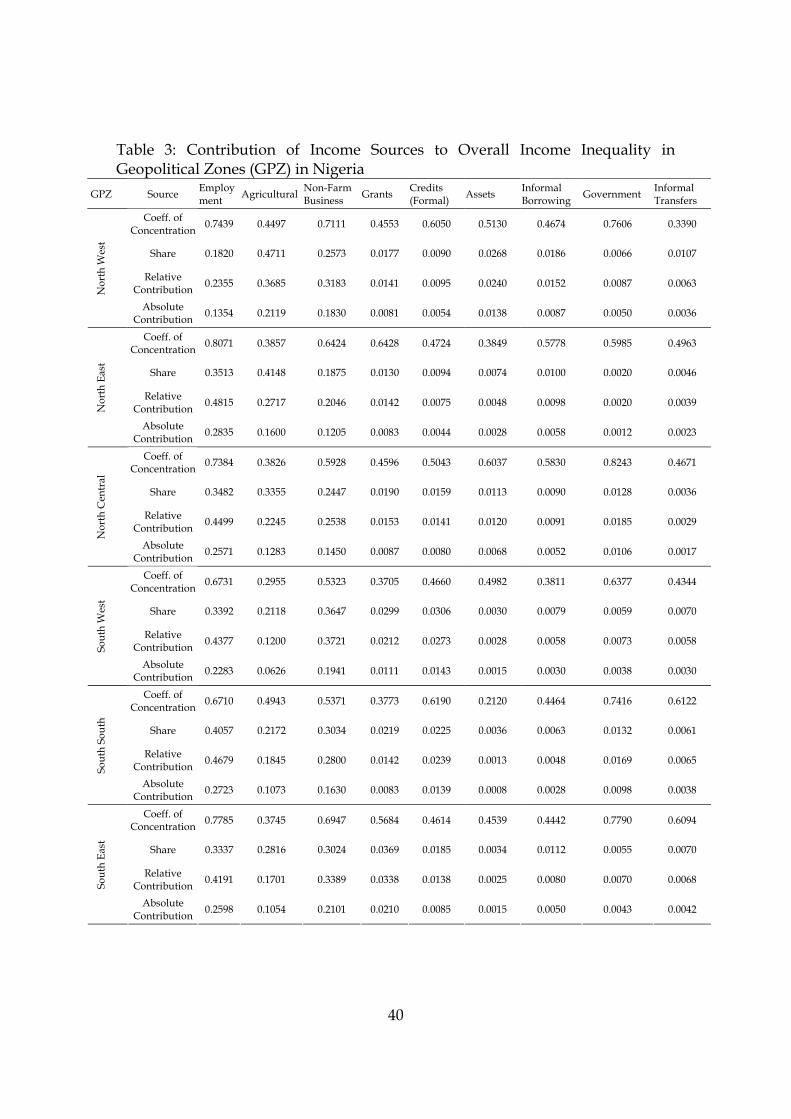
40

Table 3: Contribution of Income Sources to Overall Income Inequality in Geopolitical Zones (GPZ) in Nigeria

GPZ Source Employment Agricultural Non-Farm

Business Grants Credits (Formal) Assets Informal

Borrowing Government Informal Transfers

Coeff. of Concentration 0.7439 0.4497 0.7111 0.4553 0.6050 0.5130 0.4674 0.7606 0.3390

Share 0.1820 0.4711 0.2573 0.0177 0.0090 0.0268 0.0186 0.0066 0.0107

Relative Contribution 0.2355 0.3685 0.3183 0.0141 0.0095 0.0240 0.0152 0.0087 0.0063

Nor

th W

est

Absolute Contribution 0.1354 0.2119 0.1830 0.0081 0.0054 0.0138 0.0087 0.0050 0.0036

Coeff. of Concentration 0.8071 0.3857 0.6424 0.6428 0.4724 0.3849 0.5778 0.5985 0.4963

Share 0.3513 0.4148 0.1875 0.0130 0.0094 0.0074 0.0100 0.0020 0.0046

Relative Contribution 0.4815 0.2717 0.2046 0.0142 0.0075 0.0048 0.0098 0.0020 0.0039

N

orth

Eas

t

Absolute Contribution 0.2835 0.1600 0.1205 0.0083 0.0044 0.0028 0.0058 0.0012 0.0023

Coeff. of Concentration 0.7384 0.3826 0.5928 0.4596 0.5043 0.6037 0.5830 0.8243 0.4671

Share 0.3482 0.3355 0.2447 0.0190 0.0159 0.0113 0.0090 0.0128 0.0036

Relative Contribution 0.4499 0.2245 0.2538 0.0153 0.0141 0.0120 0.0091 0.0185 0.0029

Nor

th C

entr

al

Absolute Contribution 0.2571 0.1283 0.1450 0.0087 0.0080 0.0068 0.0052 0.0106 0.0017

Coeff. of Concentration 0.6731 0.2955 0.5323 0.3705 0.4660 0.4982 0.3811 0.6377 0.4344

Share 0.3392 0.2118 0.3647 0.0299 0.0306 0.0030 0.0079 0.0059 0.0070

Relative Contribution 0.4377 0.1200 0.3721 0.0212 0.0273 0.0028 0.0058 0.0073 0.0058

Sout

h W

est

Absolute Contribution 0.2283 0.0626 0.1941 0.0111 0.0143 0.0015 0.0030 0.0038 0.0030

Coeff. of Concentration 0.6710 0.4943 0.5371 0.3773 0.6190 0.2120 0.4464 0.7416 0.6122

Share 0.4057 0.2172 0.3034 0.0219 0.0225 0.0036 0.0063 0.0132 0.0061

Relative Contribution 0.4679 0.1845 0.2800 0.0142 0.0239 0.0013 0.0048 0.0169 0.0065

So

uth

Sout

h

Absolute Contribution 0.2723 0.1073 0.1630 0.0083 0.0139 0.0008 0.0028 0.0098 0.0038

Coeff. of Concentration 0.7785 0.3745 0.6947 0.5684 0.4614 0.4539 0.4442 0.7790 0.6094

Share 0.3337 0.2816 0.3024 0.0369 0.0185 0.0034 0.0112 0.0055 0.0070

Relative Contribution 0.4191 0.1701 0.3389 0.0338 0.0138 0.0025 0.0080 0.0070 0.0068 So

uth

East

Absolute Contribution 0.2598 0.1054 0.2101 0.0210 0.0085 0.0015 0.0050 0.0043 0.0042

41

Table 4: Contributions of Income Sources to Overall Income Inequality in Urban Nigeria

Source Coeff. of Concentration Share Relative

Contribution Absolute

Contribution

Employment 0.6184 0.4106 0.4812 0.2539

Agricultural 0.3669 0.1063 0.0739 0.0390

Non-Farm Business 0.4899 0.4028 0.3738 0.1973

Grants 0.3480 0.0257 0.0169 0.0089 Credits (Formal) 0.4842 0.0207 0.0190 0.0100

Assets 0.5949 0.0067 0.0075 0.0040 Informal Borrowing 0.4435 0.0081 0.0068 0.0036

Government 0.6578 0.0116 0.0144 0.0076

Informal Transfers

0.4472 0.0075 0.0064 0.0034

Table 5: Contributions of Income Sources to Overall Income Inequality in Rural Nigeria

Source Coeff. of

Concentration Share Relative

Contribution Absolute

Contribution Employment 0.7806 0.2582 0.3470 0.2015 Agricultural 0.4551 0.4710 0.3691 0.2143 Non-Farm Business 0.6433 0.1985 0.2198 0.1277 Grants 0.4996 0.0204 0.0175 0.0102 Credits (Formal) 0.5586 0.0168 0.0162 0.0094 Assets 0.4664 0.0121 0.0097 0.0057 Informal Borrowing 0.4878 0.0122 0.0103 0.0060 Government 0.7697 0.0048 0.0064 0.0037 Informal Transfers 0.3909 0.0060 0.0040 0.0023

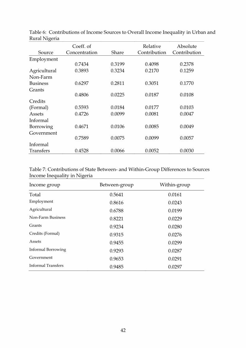
42

Table 6: Contributions of Income Sources to Overall Income Inequality in Urban and Rural Nigeria

Source Coeff. of

Concentration Share Relative

Contribution Absolute

Contribution Employment

0.7434 0.3199 0.4098 0.2378 Agricultural 0.3893 0.3234 0.2170 0.1259 Non-Farm Business 0.6297 0.2811 0.3051 0.1770 Grants

0.4806 0.0225 0.0187 0.0108 Credits (Formal) 0.5593 0.0184 0.0177 0.0103 Assets 0.4726 0.0099 0.0081 0.0047 Informal Borrowing 0.4671 0.0106 0.0085 0.0049 Government

0.7589 0.0075 0.0099 0.0057 Informal Transfers 0.4528 0.0066 0.0052 0.0030

Table 7: Contributions of State Between- and Within-Group Differences to Sources Income Inequality in Nigeria

Income group Between-group Within-group

Total 0.5641 0.0161 Employment 0.8616 0.0243 Agricultural 0.6788 0.0199 Non-Farm Business 0.8221 0.0229 Grants 0.9234 0.0280 Credits (Formal) 0.9315 0.0276 Assets 0.9455 0.0299 Informal Borrowing 0.9293 0.0287 Government 0.9653 0.0291 Informal Transfers 0.9485 0.0297

43

Table 8: Urban-Rural Between- and Within-Group Sources of Inequality in Income in Nigeria

Rural Urban Between-Group Within-group

Total 0.2522 0.0578 0.2702 0.3100

Employment 0.3214 0.1124 0.4520 0.4338

Agricultural 0.4013 0.0313 0.2661 0.4326

Non-Farm Business 0.2709 0.1133 0.4608 0.3842 Grants 0.3744 0.1173 0.4597 0.4916

Credits (Formal) 0.3818 0.1169 0.4604 0.4987

Assets 0.5139 0.0729 0.3887 0.5868

Informal Borrowing 0.4787 0.0816 0.3977 0.5603

Government 0.2754 0.1662 0.5529 0.4415

Informal Transfers 0.3809 0.1231 0.4742 0.5040 Table 9: Between- and Within-Group Inequality in Income Sources in Geopolitical Zones in Nigeria

Income Source/GPZ North West North East North Central South West South

South South East Between-Group

Within-group

Total 0.0254 0.0154 0.0202 0.0254 0.0071 0.0066 0.4801 0.1001

Employment 0.0234 0.0259 0.0338 0.0434 0.0127 0.0100 0.7366 0.1492

Agricultural 0.0413 0.0212 0.0254 0.0238 0.0066 0.0065 0.5740 0.1247

Non-Farm Business 0.0359 0.0156 0.0261 0.0475 0.0103 0.0100 0.6995 0.1454

Grants 0.0328 0.0147 0.0285 0.0599 0.0112 0.0166 0.7877 0.1636

Credits (Formal) 0.0212 0.0128 0.0295 0.0746 0.0143 0.0102 0.7965 0.1626

Assets 0.1131 0.0189 0.0395 0.0144 0.0044 0.0036 0.7816 0.1939

Informal Borrowing 0.0723 0.0239 0.0290 0.0350 0.0070 0.0109 0.7800 0.1780

Government 0.0382 0.0069 0.0596 0.0380 0.0212 0.0078 0.8227 0.1717

Informal Transfers 0.0678 0.0181 0.0189 0.0508 0.0112 0.0111 0.8002 0.1780

44

Table 10a: Regression Based Decomposition of Sources of Income Inequality in Urban and Rural Nigeria

Per capita household income Per capita household adult equivalent income

Variables Coefficient T statistics Tolerance Contribution Coefficient T statistics Tolerance Contribution

Constant 27042.0320 8.0850 30117.2920 6.9240

Regional and sector

Sector 6030.7330 7.7300 0.6760 0.0153 6370.5090 6.2780 0.6760 0.0122

Born here 342.8750 0.4580 0.8950 -0.0001 433.3910 0.4450 0.8950 -0.0001 Always live here 345.1740 0.3000 0.9220 0.0000 -64.6770 -0.0430 0.9220 0.0000

South west 10007.1580 11.8580 0.7530 0.0233 13819.6620 12.5910 0.7530 0.0242 South east and south south -3083.0430 -4.2010 0.8510 0.0012 -5336.4220 -5.5900 0.8510 0.0022 Socio-economic

Household size -3224.3040 -30.9210 0.8530 0.0564 -2496.3180 -18.4070 0.8530 0.0204

Education 2288.1420 3.5790 0.8450 0.0011 2960.3160 3.5600 0.8450 0.0011 Father’s education 257.1200 0.0980 0.9780 0.0000 -2243.1070 -0.6600 0.9780 0.0000 Mother education 4060.3830 3.1590 0.9680 0.0010 5577.1180 3.3360 0.9680 0.0010

Sex 1058.3820 1.1880 0.8870 0.0000 -641.4720 -0.5530 0.8870 0.0000

Age 12.9690 0.6000 0.8570 -0.0001 5.4920 0.1950 0.8570 0.0000 Marital status -3542.7420 -3.2770 0.8510 0.0008 -4051.9530 -2.8820 0.8510 0.0004

Religion -1434.9830 -2.3240 0.8510 0.0001 -1765.4070 -2.1980 0.8510 0.0001 Father at home -1923.8890 -1.0830 0.9710 0.0000 -1499.8980 -0.6490 0.9710 0.0000 Mother at home -1140.8690 -0.8640 0.9570 0.0002 -1067.5750 -0.6220 0.9570 0.0001 Times of illness -219.8140 -2.1110 0.9770 0.0002 -341.5070 -2.5220 0.9770 0.0003

Occupation and capital

Paid job 22515.8010 31.7830 0.8140 0.0673 28668.0080 31.1150 0.8140 0.0671

Farming -1978.6540 -2.6340 0.6320 0.0055 -2091.4580 -2.1400 0.6320 0.0042

Non farm business 8889.1510 13.5670 0.7920 0.0140 13183.5730 15.4710 0.7920 0.0190

Grants 0.2760 15.6180 0.9890 0.0156 0.3720 16.2120 0.9890 0.0174 Formal Credit 0.2940 13.0200 0.9710 0.0126 0.3950 13.4550 0.9710 0.0143

Asset 0.1670 6.3470 0.9920 0.0012 0.2070 6.0510 0.9920 0.0014

Informal Credit 0.3330 9.4620 0.9820 0.0049 0.4580 10.0120 0.9820 0.0062

Residual 0.7793 0.8084

45

Table 10b: Regression Based Decomposition of Sources of Income Inequality in Urban Nigeria

Per capita household income Per capita household adult equivalent income Variables

Coefficient T statistics Tolerance Contribution Coefficient T

Statistics Tolerance Contribution Constant 42778.8730 4.8860 60005.3310 5.3890

Regional factors

Born here 671.8350 0.3770 0.8640 0.0000 1152.8760 0.5090 0.8640 0.0000 Always live here 2290.4230 0.8200 0.9120 0.0001 -964.3340 -0.2710 0.9120 0.0000

South west 4292.9980 2.5870 0.7450 0.0062 4413.8340 2.1030 0.7540 0.0050 South east and south south -6063.3680 -2.9020 0.7870 0.0026 -11195.9390 -4.2160 0.7880 0.0050 Socio-economic

Household size -4686.0600 -18.3480 0.8270 0.0768 -7417.0960 -18.3680 0.8540 0.0717

Education 4626.4200 2.9040 0.8350 0.0018 7252.4770 3.5790 0.8350 0.0024 Father’s education -5560.5670 -0.8410 0.9790 0.0001 -16863.5600 -2.0040 0.9790 0.0008 Mother education 5438.9750 1.6330 0.9680 0.0011 6029.5410 1.4250 0.9700 0.0008

Sex -313.6790 -0.1450 0.8920 0.0000 -2498.7930 -0.9060 0.8920 0.0000

Age 34.8630 0.6540 0.8530 -0.0003 130.0150 1.9180 0.8520 -0.0002 Marital status -4736.0880 -1.6900 0.8390 0.0008 -4594.2850 -1.2900 0.8400 0.0004

Religion -2821.4180 -1.8020 0.8150 0.0005 -3459.0660 -1.7370 0.8150 0.0003 Father at home -1074.7550 -0.2460 0.9470 0.0000 2750.0700 0.4960 0.9470 0.0001 Mother at home -1623.8550 -0.4430 0.9410 0.0002 163.8780 0.0350 0.9420 0.0000 Times of illness -691.7320 -2.6870 0.9710 0.0017 -953.4310 -2.9120 0.9710 0.0018

Occupation and capital

Paid job 26014.3950 15.6860 0.7320 0.0481 34495.0250 16.3980 0.7360 0.0484

Farming -1662.7570 -0.9930 0.8750 0.0015 -210.6260 -0.1000 0.8870 0.0001

Non farm business 12356.7360 7.2760 0.7220 0.0005 18612.3120 8.6730 0.7320 0.0044

Grants 0.2550 7.7070 0.9900 0.0126 0.3940 9.3740 0.9900 0.0184 Formal Credit 0.2590 6.4860 0.9680 0.0097 0.3780 7.4410 0.9680 0.0131

Asset 0.1570 3.2850 0.9930 0.0011 0.1960 3.2240 0.9940 0.0011

Informal Credit 0.2530 3.9000 0.9810 0.0025 0.4840 5.8680 0.9830 0.0066

Residual 0.8323 0.8196

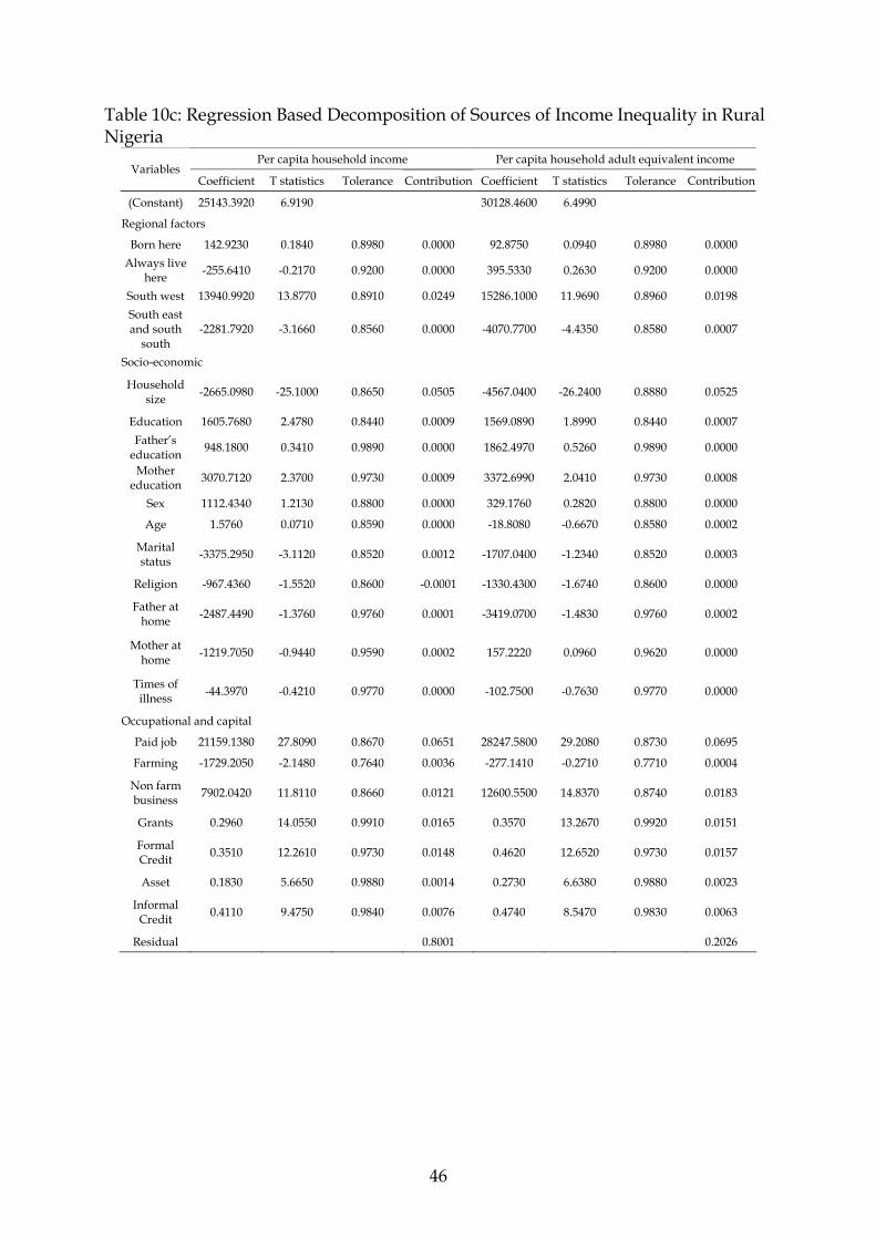
46

Table 10c: Regression Based Decomposition of Sources of Income Inequality in Rural Nigeria

Per capita household income Per capita household adult equivalent income Variables

Coefficient T statistics Tolerance Contribution Coefficient T statistics Tolerance Contribution

(Constant) 25143.3920 6.9190 30128.4600 6.4990

Regional factors

Born here 142.9230 0.1840 0.8980 0.0000 92.8750 0.0940 0.8980 0.0000 Always live

here -255.6410 -0.2170 0.9200 0.0000 395.5330 0.2630 0.9200 0.0000

South west 13940.9920 13.8770 0.8910 0.0249 15286.1000 11.9690 0.8960 0.0198 South east and south

south -2281.7920 -3.1660 0.8560 0.0000 -4070.7700 -4.4350 0.8580 0.0007

Socio-economic

Household size -2665.0980 -25.1000 0.8650 0.0505 -4567.0400 -26.2400 0.8880 0.0525

Education 1605.7680 2.4780 0.8440 0.0009 1569.0890 1.8990 0.8440 0.0007 Father’s

education 948.1800 0.3410 0.9890 0.0000 1862.4970 0.5260 0.9890 0.0000

Mother education 3070.7120 2.3700 0.9730 0.0009 3372.6990 2.0410 0.9730 0.0008

Sex 1112.4340 1.2130 0.8800 0.0000 329.1760 0.2820 0.8800 0.0000

Age 1.5760 0.0710 0.8590 0.0000 -18.8080 -0.6670 0.8580 0.0002

Marital status -3375.2950 -3.1120 0.8520 0.0012 -1707.0400 -1.2340 0.8520 0.0003

Religion -967.4360 -1.5520 0.8600 -0.0001 -1330.4300 -1.6740 0.8600 0.0000

Father at home -2487.4490 -1.3760 0.9760 0.0001 -3419.0700 -1.4830 0.9760 0.0002

Mother at home -1219.7050 -0.9440 0.9590 0.0002 157.2220 0.0960 0.9620 0.0000

Times of illness -44.3970 -0.4210 0.9770 0.0000 -102.7500 -0.7630 0.9770 0.0000

Occupational and capital

Paid job 21159.1380 27.8090 0.8670 0.0651 28247.5800 29.2080 0.8730 0.0695

Farming -1729.2050 -2.1480 0.7640 0.0036 -277.1410 -0.2710 0.7710 0.0004

Non farm business 7902.0420 11.8110 0.8660 0.0121 12600.5500 14.8370 0.8740 0.0183

Grants 0.2960 14.0550 0.9910 0.0165 0.3570 13.2670 0.9920 0.0151

Formal Credit 0.3510 12.2610 0.9730 0.0148 0.4620 12.6520 0.9730 0.0157

Asset 0.1830 5.6650 0.9880 0.0014 0.2730 6.6380 0.9880 0.0023

Informal Credit 0.4110 9.4750 0.9840 0.0076 0.4740 8.5470 0.9830 0.0063

Residual 0.8001 0.2026

47

Table 11: Decomposition of Change in Poverty Incidence in Nigeria into Income Growth and Redistribution Between 1998 and 2004

Datts and Ravallion Shapley State/sector

% Growth in Real Income

Absolute change in

Gini

1998 poverty incidence

2004 poverty incidence Difference

Growth Redistribution Residual Growth Redistribution

All (CAS) -13.0891 0.1121 0.4051 0.5159 0.1108 0.0595 0.0682 -0.0168 0.0511 0.0597 Urban 16.2114 0.1041 0.2968 0.3161 0.0193 -0.0535 0.0557 0.0171 -0.0449 0.0642 Rural -26.3098 0.0982 0.4452 0.5900 0.1448 0.1394 0.0422 -0.0368 0.1210 0.0238 North West -6.7260 0.0256 0.6394 0.6623 0.0229 0.0323 -0.0014 -0.0080 0.0283 -0.0054 Jigawa -49.5846 0.2483 0.6967 0.8695 0.1727 0.2457 -0.0307 -0.0422 0.2246 -0.0518 Kaduna -1.4002 0.1239 0.3944 0.5219 0.1275 0.0179 0.1215 -0.0120 0.0120 0.1155 Kano 8.3016 -0.2251 0.6330 0.5243 -0.1086 -0.0506 -0.0861 0.0281 -0.0365 -0.0721 Katsina 3.3369 0.0896 0.6673 0.6557 -0.0116 -0.0135 -0.0039 0.0058 -0.0106 -0.0010 Kebbi -33.5611 0.0333 0.8151 0.8366 0.0215 0.0839 -0.1247 0.0624 0.1151 -0.0935 Sokoto -9.7414 0.2839 0.6109 0.6652 0.0543 0.0385 0.0136 0.0023 0.0396 0.0147 Zamfara 21.6864 0.2595 0.6647 0.5795 -0.0853 -0.1260 -0.0349 0.0756 -0.0882 0.0029 North East 2.5000 0.1600 0.5379 0.5561 0.0182 -0.0159 0.0258 0.0083 -0.0117 0.0299 Adamawa -57.0007 0.3181 0.4323 0.7838 0.3515 0.3325 0.1544 -0.1354 0.2648 0.0867 Bauchi 26.7332 0.1262 0.3351 0.2815 -0.0536 -0.1153 0.0027 0.0590 -0.0858 0.0322 Borno 45.0371 0.2840 0.3103 0.3218 0.0115 -0.1897 0.0690 0.1322 -0.1236 0.1351 Gombe 3.0060 0.1843 0.5944 0.5987 0.0043 -0.0260 0.0217 0.0087 -0.0217 0.0260 Taraba -13.6393 0.0701 0.5281 0.5843 0.0562 0.0169 0.0056 0.0337 0.0337 0.0225 Yobe 81.2360 0.1264 0.7871 0.5778 -0.2093 -0.2469 0.0036 0.0340 -0.2299 0.0206 North Central -27.2472 0.0932 0.3502 0.5106 0.1604 0.1522 0.0532 -0.0451 0.1297 0.0307 Benue -73.2798 0.2270 0.0133 0.5733 0.5600 0.5867 0.2400 -0.2667 0.4533 0.1067 Kogi -42.9619 0.1451 0.4644 0.5686 0.1042 0.2303 -0.1188 -0.0073 0.2267 -0.1225 Kwara 1.6092 0.0136 0.2702 0.3886 0.1183 -0.0059 0.1243 0.0000 -0.0059 0.1243 Nasarawa -38.7319 0.1843 0.2694 0.6142 0.3447 0.2306 0.2009 -0.0868 0.1872 0.1575 Niger 15.3350 0.1193 0.4859 0.4615 -0.0244 -0.0769 0.0150 0.0375 -0.0582 0.0338 Plateau -34.2122 0.0767 0.3069 0.4802 0.1733 0.2088 0.0209 -0.0564 0.1806 -0.0073 FCT -42.1667 0.0626 0.2971 0.5983 0.3013 0.2552 0.0837 -0.0377 0.2364 0.0649 South West 9.0141 0.1011 0.1580 0.2392 0.0811 -0.0315 0.0974 0.0152 -0.0239 0.1051 Ekiti 3.6041 0.1067 0.2529 0.3503 0.0974 -0.0023 0.1044 -0.0046 -0.0046 0.1021 Lagos -20.8836 0.0885 0.0261 0.1540 0.1280 0.0355 0.1043 -0.0118 0.0296 0.0983 Ogun 13.3178 0.1299 0.1766 0.3224 0.1458 -0.0349 0.1910 -0.0103 -0.0400 0.1858 Ondo 41.1465 0.1385 0.2806 0.2325 -0.0481 -0.1563 0.0401 0.0681 -0.1222 0.0741 Osun 22.6298 0.0910 0.0885 0.1650 0.0765 -0.0463 0.1187 0.0040 -0.0443 0.1207 Oyo 15.0428 0.1036 0.1152 0.2140 0.0988 -0.0535 0.1132 0.0391 -0.0340 0.1327 South South -22.6170 0.2384 0.2672 0.4717 0.2045 0.1448 0.1411 -0.0814 0.1041 0.1004 Akwa Ibom -27.1612 0.3762 0.2313 0.5053 0.2740 0.2171 0.1993 -0.1423 0.1459 0.1281 Bayelsa 130.8553 0.3956 0.8296 0.6222 -0.2074 -0.4296 -0.0667 0.2889 -0.2852 0.0778 Cross Rivers -70.6929 0.1840 0.2374 0.5468 0.3094 0.4820 -0.0072 -0.1655 0.3993 -0.0899 Delta -55.5392 0.3172 0.0781 0.4740 0.3958 0.4479 0.2448 -0.2969 0.2995 0.0964 Edo -24.0933 0.3148 0.2123 0.5496 0.3373 0.1885 0.2619 -0.1131 0.1319 0.2054 Rivers 27.7805 0.0319 0.2737 0.2486 -0.0251 -0.1089 0.0140 0.0698 -0.0740 0.0489 South East -42.9784 0.2068 0.3618 0.6510 0.2892 0.2433 0.1393 -0.0934 0.1966 0.0926 Abia -54.7825 0.3313 0.0349 0.4922 0.4574 0.3333 0.2791 -0.1550 0.2558 0.2016 Anambra -60.7804 0.2537 0.0082 0.4221 0.4139 0.3443 0.2295 -0.1598 0.2643 0.1496 Ebonyi -60.4921 0.1910 0.5879 0.9024 0.3145 0.2907 0.0651 -0.0412 0.2701 0.0445 Enugu 14.0008 0.2618 0.6004 0.6522 0.0518 -0.0518 0.0932 0.0104 -0.0466 0.0983 Imo -23.0754 0.3273 0.2459 0.6066 0.3607 0.1710 0.2927 -0.1030 0.1194 0.2412

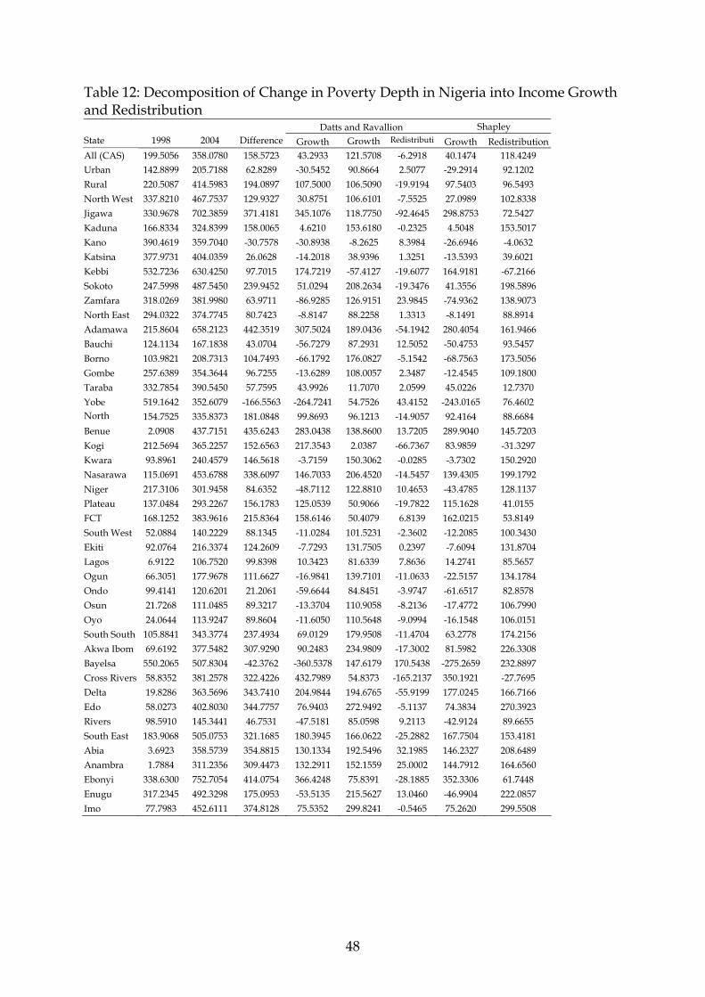
48

Table 12: Decomposition of Change in Poverty Depth in Nigeria into Income Growth and Redistribution

Datts and Ravallion Shapley State 1998 2004 Difference Growth Growth Redistributi

Growth Redistribution

All (CAS) 199.5056 358.0780 158.5723 43.2933 121.5708 -6.2918 40.1474 118.4249 Urban 142.8899 205.7188 62.8289 -30.5452 90.8664 2.5077 -29.2914 92.1202 Rural 220.5087 414.5983 194.0897 107.5000 106.5090 -19.9194 97.5403 96.5493 North West 337.8210 467.7537 129.9327 30.8751 106.6101 -7.5525 27.0989 102.8338 Jigawa 330.9678 702.3859 371.4181 345.1076 118.7750 -92.4645 298.8753 72.5427 Kaduna 166.8334 324.8399 158.0065 4.6210 153.6180 -0.2325 4.5048 153.5017 Kano 390.4619 359.7040 -30.7578 -30.8938 -8.2625 8.3984 -26.6946 -4.0632 Katsina 377.9731 404.0359 26.0628 -14.2018 38.9396 1.3251 -13.5393 39.6021 Kebbi 532.7236 630.4250 97.7015 174.7219 -57.4127 -19.6077 164.9181 -67.2166 Sokoto 247.5998 487.5450 239.9452 51.0294 208.2634 -19.3476 41.3556 198.5896 Zamfara 318.0269 381.9980 63.9711 -86.9285 126.9151 23.9845 -74.9362 138.9073 North East 294.0322 374.7745 80.7423 -8.8147 88.2258 1.3313 -8.1491 88.8914 Adamawa 215.8604 658.2123 442.3519 307.5024 189.0436 -54.1942 280.4054 161.9466 Bauchi 124.1134 167.1838 43.0704 -56.7279 87.2931 12.5052 -50.4753 93.5457 Borno 103.9821 208.7313 104.7493 -66.1792 176.0827 -5.1542 -68.7563 173.5056 Gombe 257.6389 354.3644 96.7255 -13.6289 108.0057 2.3487 -12.4545 109.1800 Taraba 332.7854 390.5450 57.7595 43.9926 11.7070 2.0599 45.0226 12.7370 Yobe 519.1642 352.6079 -166.5563 -264.7241 54.7526 43.4152 -243.0165 76.4602 North 154.7525 335.8373 181.0848 99.8693 96.1213 -14.9057 92.4164 88.6684 Benue 2.0908 437.7151 435.6243 283.0438 138.8600 13.7205 289.9040 145.7203 Kogi 212.5694 365.2257 152.6563 217.3543 2.0387 -66.7367 83.9859 -31.3297 Kwara 93.8961 240.4579 146.5618 -3.7159 150.3062 -0.0285 -3.7302 150.2920 Nasarawa 115.0691 453.6788 338.6097 146.7033 206.4520 -14.5457 139.4305 199.1792 Niger 217.3106 301.9458 84.6352 -48.7112 122.8810 10.4653 -43.4785 128.1137 Plateau 137.0484 293.2267 156.1783 125.0539 50.9066 -19.7822 115.1628 41.0155 FCT 168.1252 383.9616 215.8364 158.6146 50.4079 6.8139 162.0215 53.8149 South West 52.0884 140.2229 88.1345 -11.0284 101.5231 -2.3602 -12.2085 100.3430 Ekiti 92.0764 216.3374 124.2609 -7.7293 131.7505 0.2397 -7.6094 131.8704 Lagos 6.9122 106.7520 99.8398 10.3423 81.6339 7.8636 14.2741 85.5657 Ogun 66.3051 177.9678 111.6627 -16.9841 139.7101 -11.0633 -22.5157 134.1784 Ondo 99.4141 120.6201 21.2061 -59.6644 84.8451 -3.9747 -61.6517 82.8578 Osun 21.7268 111.0485 89.3217 -13.3704 110.9058 -8.2136 -17.4772 106.7990 Oyo 24.0644 113.9247 89.8604 -11.6050 110.5648 -9.0994 -16.1548 106.0151 South South 105.8841 343.3774 237.4934 69.0129 179.9508 -11.4704 63.2778 174.2156 Akwa Ibom 69.6192 377.5482 307.9290 90.2483 234.9809 -17.3002 81.5982 226.3308 Bayelsa 550.2065 507.8304 -42.3762 -360.5378 147.6179 170.5438 -275.2659 232.8897 Cross Rivers 58.8352 381.2578 322.4226 432.7989 54.8373 -165.2137 350.1921 -27.7695 Delta 19.8286 363.5696 343.7410 204.9844 194.6765 -55.9199 177.0245 166.7166 Edo 58.0273 402.8030 344.7757 76.9403 272.9492 -5.1137 74.3834 270.3923 Rivers 98.5910 145.3441 46.7531 -47.5181 85.0598 9.2113 -42.9124 89.6655 South East 183.9068 505.0753 321.1685 180.3945 166.0622 -25.2882 167.7504 153.4181 Abia 3.6923 358.5739 354.8815 130.1334 192.5496 32.1985 146.2327 208.6489 Anambra 1.7884 311.2356 309.4473 132.2911 152.1559 25.0002 144.7912 164.6560 Ebonyi 338.6300 752.7054 414.0754 366.4248 75.8391 -28.1885 352.3306 61.7448 Enugu 317.2345 492.3298 175.0953 -53.5135 215.5627 13.0460 -46.9904 222.0857 Imo 77.7983 452.6111 374.8128 75.5352 299.8241 -0.5465 75.2620 299.5508

49

Appendix 1: Income Share, Inequality and Consumer Price Indices in Nigeria State/zone Growth in

real income (%)

Gini of 1998 real

income

Gini of 2004 real income

Gini of 1998

Nominal Income

Gini of 2004

Nominal income

Average Price Index

Mean Income

Income share (%)

Population share (%)

All -13.0891 0.4643 0.5765 0.4501 0.5802 - Abia -54.7825 0.2252 0.5565 0.2303 0.5589 1.2300 90605.3251 1.4184 1.7040 Adamawa -57.0007 0.4009 0.7190 0.4029 0.7021 1.0460 67861.2936 1.7335 2.7805 Akwa ibom -27.1612 0.2111 0.5873 0.2307 0.5732 1.2637 110058.0384 1.8765 1.8559 Anambra -60.7804 0.3211 0.5748 0.3424 0.5600 1.2620 129679.1454 1.9199 1.6115 Bayelsa 130.8553 0.2254 0.6210 0.2229 0.6214 0.9229 132462.7998 1.0851 0.8916 Bauchi 26.7332 0.2994 0.4256 0.2907 0.4012 1.3628 102158.3986 2.3121 2.4635 Benue -73.2798 0.3258 0.5528 0.3223 0.5871 0.9277 100810.7418 0.4588 0.4953 Borno 45.0371 0.2337 0.5177 0.2190 0.5283 0.9845 201526.9843 2.1277 1.1492 Cross river -70.6929 0.3103 0.4943 0.3804 0.5409 1.2725 83268.0935 0.7023 0.9180 Delta -55.5392 0.2316 0.5489 0.2469 0.5653 1.3796 94383.9269 1.0996 1.2681 Ebonyi -60.4921 0.3147 0.5057 0.3151 0.5179 1.1305 30862.9322 0.8633 3.0447 Edo -24.0933 0.2586 0.5735 0.2389 0.5899 1.3470 84122.1879 2.5726 3.3287 Ekiti 3.6041 0.3818 0.4885 0.4113 0.4901 1.0050 92555.6180 2.4205 2.8466 Enugu 14.0008 0.3306 0.5925 0.3280 0.6046 1.1152 77126.3551 2.2603 3.1900 Gombe 3.0060 0.3237 0.5080 0.3057 0.4986 0.9886 83245.0216 2.3285 3.0447 Imo -23.0754 0.2790 0.6064 0.2694 0.6268 1.0668 81417.7222 2.1095 2.8202 Jigawa -49.5846 0.3227 0.5711 0.3249 0.5768 0.8551 52561.0862 1.6616 3.4410 Kaduna -1.4002 0.3837 0.5075 0.3691 0.5049 0.9212 117233.5962 3.5709 3.3155 Kano 8.3016 0.7218 0.4967 0.6281 0.5004 0.8736 108581.9745 3.5182 3.5268 Katsina 3.3369 0.4349 0.5245 0.4003 0.5189 0.9281 92375.8146 2.8978 3.4146 Kebbi -33.5611 0.5272 0.5605 0.5587 0.5502 1.0477 49878.9636 1.4073 3.0711 Kogi -42.9619 0.4054 0.5505 0.4796 0.5709 1.0868 85837.1082 2.8490 3.6127 Kwara 1.6092 0.5250 0.5386 0.4836 0.5464 0.8875 124554.7370 3.8317 3.3485 Lagos -20.8836 0.3495 0.4379 0.3490 0.4508 1.1806 213705.7394 5.4721 2.7871 Nasarawa -38.7319 0.4148 0.5991 0.4057 0.6130 0.9291 115210.4062 3.0619 2.8928 Niger 15.3350 0.4327 0.5519 0.4345 0.5658 0.9840 111373.2931 3.6019 3.5202 Ogun 13.3178 0.3808 0.5107 0.3934 0.5446 1.0549 112524.7336 3.3251 3.2164 Ondo 41.1465 0.3285 0.4669 0.3633 0.4854 1.0907 127382.8757 3.8569 3.2957 Osun 22.6298 0.3845 0.4756 0.3681 0.5086 0.9281 177038.7548 5.3389 3.2825 Oyo 15.0428 0.3810 0.4846 0.3626 0.5186 0.9733 193368.6151 5.7022 3.2098 Plateau -34.2122 0.4334 0.5101 0.4270 0.5353 0.9129 126834.8656 3.6864 3.1636 Rivers 27.7805 0.4250 0.4569 0.4095 0.5042 1.4592 189354.3660 4.1132 2.3644 Sokoto -9.7414 0.3180 0.6020 0.3388 0.6198 1.0089 88420.1156 2.3714 2.9192 Taraba -13.6393 0.5217 0.5917 0.5248 0.6519 0.9765 126775.1491 4.1077 3.5268 Yobe 81.2360 0.3842 0.5106 0.3439 0.5332 0.9930 92393.1696 3.1338 3.6920 Zamfara 21.6864 0.3481 0.6076 0.3624 0.6052 1.0119 118416.2041 3.7075 3.4080 FCT -42.1667 0.5153 0.5779 0.5215 0.5806 1.3603 103168.8361 1.4961 1.5785 North west -6.7260 0.5489 0.5744 0.4814 0.5749 - 90178.6766 19.1348 23.0962 North east 2.5000 0.4295 0.5895 0.4316 0.5889 - 102808.5133 15.7263 16.6502 North centra -27.2472 0.4642 0.5574 0.4760 0.5716 - 111035.6036 18.9857 18.6117

South west 9.0141 0.3960 0.4971 0.4028 0.5217 - 152517.4705 26.1156 18.6381

South south -22.6170 0.3308 0.5692 0.3258 0.5819 - 117272.3502 11.4492 10.6268

South east -42.9784 0.4079 0.6147 0.4158 0.6198 - 75530.8863 8.5885 12.3770

Urban 16.2114 0.4132 0.5173 0.4065 0.5278 - 162768.3443 40.4631 27.0590

Rural -26.3098 0.4799 0.5781 0.4649 0.5808 - 88845.7002 59.5369 72.9410