exclusion and discrimination as sources of inter …manuelb/research/exclusion and... · manuel...

Economía Vol. XXXI, N° 61, semestre enero-junio 2008, pp. 51-80 / ISSN 0254-4415

Exclusion and Discrimination as Sources of Inter-Ethnic Inequality in Peru*

Manuel Barrón** IFPRI

RESUMEN

De acuerdo a la Enaho 2003, el ingreso promedio de un trabajador indígena es solo 56% del de un trabajador no-indígena. Sin embargo, estudios sobre discriminación étnica en los mercados laborales de Perú usualmente hallan brechas demasiado pequeñas como para explicar la desigualdad observada. De acuerdo a Figueroa (2003), la exclusión social es una fuente importante de desigualdad interétnica, pero esto no ha sido contrastado empíricamente. El objetivo central de este documento es llenar esa brecha estimando qué porcentaje de la desigualdad se debe a exclusión y qué porcentaje a discriminación, comparando directamente los efectos. La metodología econométrica utilizada (hurdlemodels)permite incluir en el análisis a los trabajadores con ingresos nulos y contrarrestar problemas de endogeneidad econométrica. Los resultados implican que la exclusión juega un papel más importante que la discriminación. Sin exclusión, el Gini de ingresos laborales se reduciría de 0.64 a cerca de 0.45; sin discriminación, a alrededor de 0.50.Palabrasclave:desigualdad interétnica, exclusión, hurdlemodels.

ABSTRACT

According to the 2003 National Household Survey, mean labour income for an indigenous worker is only 56% of that for a non-indigenous worker. Studies of ethnic discrimination in Peru’s labour markets generally find that discrimination is too low to explain inequalities of this magnitude. However, Sigma Theory (Figueroa 2003) predicts that social exclusion is a source of inter-ethnic inequality, and that has not been empirically tested. The primary aim of this paper is to fill this gap by estimating the extent to which exclusion and discrimination contribute to income inequality. Hurdle models are used to tackle down econometric endogeneity of years of schooling and truncation-at-zero of incomes. The results imply that exclusion plays a stronger role on inequality than discrimination: without exclusion, the Gini of labour income would decrease from 0.64 to 0.45, and without discrimination it would be reduced to 0.50.Keywords:inter-ethnic inequality, exclusion, hurdle models.

JEL Codes: C24, J31, o15

* This paper is based on the thesis submitted in partial fulfilment of the degree of Master of Science in Economics for Development at the University of oxford, June 2006. I am grateful to Sudhir Anand, Mans Soderbom, and the anonymous referees for their insightful comments. All errors and omissions are my own.** International Food Policy Research Institute. Contact address: [email protected].

52 Economía Vol. XXXI, N° 61, 2008 / ISSN 0254-4415

INTRoDUCTIoN

Several studies have tried to measure the degree of ethnic discrimination in Peru’s labour markets (see for example Trivelli 2005, Figueroa and Barrón 2005, Barrón 2005, Ñopo etal. 2004, Mc Isaac 1994), generally finding little discrimination if any at all. However, according to the National Household Survey of 2003, mean labour income for an indigenous worker is only 56% of that for a non-indigenous worker. As shown in section 4, for the expected value of lifetime labour income, the figure is 44%. In addition, Peru systematically shows very high inequality indices (Gini and Theil’s T measure for incomes of around 0.55 and 0.80, respectively). Since discrimination does not appear to play an important role in this outcome, exclusion must be the main driver of inequality, but that hasn’t been properly addressed in the literature. The primary aim of this paper is to fill this gap by estimating the extent to which exclusion and discrimination contribute to income inequality and compare their effects directly.

A further contribution of this paper is the implementation of an econometric methodology to obtain unbiased estimates of the determinants of labour income. Two problems arise in the estimation: in first place, education is likely to suffer of econometric endogeneity; and in second place an important share of workers is unpaid, and thus the distribution of incomes is truncated at zero, therefore non-normality in the distribution of the endogenous variable arises. Even though the first problem is usually taken into account, the second problem is not discussed in the literature. A two-tiered or «hurdle model» is used to asses these problems. The first tier assesses the probability of having positive dependent variable and the second one estimates the expected value of the dependent variable given that it is positive. Three methodologies were used to address the problem of econometric endogeneity in the second tier: instrumental variables, proxy variables, and household fixed effects.

1. HISToRICAL BACKGRoUND

Latin America is the most unequal regions of the world (Deininger and Squire 1996; Li etal. 1997). A recent current of economic history has focused on the relationship between inequality and the colonial past of Latin American countries (e.g. Engerman and Sokoloff 2002, Acemoglu etal. 2002, Mahoney 2003). These authors share the idea that the dynamics of inequality are driven by inertia, meaning that current inequality depends on past inequality, process that has been called «path dependence». Inequality is the heaviest burden from Latin America’s colonial past.

Where indigenous population was dense, political elites excluded broad spectrums of society from the basic entitlements of citizenship (Mahoney 2003). This lead to inequality in factor endowments, which is profound determinant of the type of institutions that emerge in a society (Engerman and Sokoloff 2002). Where initial inequality was high,

Manuel Barrón ExclusionandDiscriminationasSourcesofInter-EthnicInequalityinPeru 53

elites were in a better position to establish legal frameworks that would guarantee political power and economic opportunities. In this type of societies, the result is the establishment of extractive institutions rather than industrialisation, which in turn, reproduce high inequality (Acemoglu etal. 2002).

Summing up the different approaches, it may be argued that the indigenous density (the share of indigenous people in total population) determined the width of citizenship, which, in turn, determined the type of institutions that prevailed in the society. These institutions determined public policies regarding education, land, and health, as well as fiscal and monetary policies (tax system, social assistance programs, etc.); which set incentives in favour of either extractive activities or industrialisation. While the formers reproduce high inequality, the latter reproduces relatively low inequality. Hence, the initial share of indigenous population was a determinant of the degree of inequality. New questions arise now. What factors determined the density of indigenous population before the arrival of the Spaniards? Was it economic prosperity of the different regions? or maybe central planning decisions by the corresponding empire? The answers to these questions constitute very interesting and challenging issues to pin down, but are beyond the scope of this study.

With the Spanish invasion, indigenous peoples went through a number of economic shocks over and above social degradation. In first place, they experienced a major demographic shock because of the diseases carried by the Spaniards, for which they did not have developed antibodies (Diamond 1997). In second place, labour was relocated massively from agriculture to mining, according to the main interest of the Spaniards. At the same time, indigenous people were expelled from the most productive lands, being left with the least productive or with none at all. These shocks in the main means of production (labour and land) originated severe disequilibria, and hence serious inefficiencies, which agglutinated the indigenous peoples in the poorest clusters of society. Moreover, their economic system (based on reciprocity and redistribution) was abruptly replaced by the Spanish, where the State was a fierce tax collector with practically no redistribution to the people.1

In addition, indigenous people were excluded from formal education, literacy being an exceptional characteristic amongst them. By doing so, the Spaniards blocked their access to human capital, thus impeding their entrance to the modern sector of the economy and confining them to extractive activities.

Independence came after almost three centuries, but nothing changed for indigenous peoples in Latin America (Albó 2002). Literacy and landholding were conditions to vote

1 In the case of Peru, the so-called «indigenous tax» was one of the main sources of income during the time of the Viceroyalty, as well as during the first phase of the Republic. After being abolished and almost imme-diately reestablished several times, it was definitively eliminated during the government of Ramón Castilla during an economic boom driven by guano exports. For a more detailed discussion of the indigenous tax in Peru, see Estela (2001).


and to run for public posts. This meant that the majority of indigenous people was excluded from electing the political authorities, but also that indigenous authorities were not able to get a place in the formal political system. Their exclusion was based on the grounds that indigenous did not have capacity of organisation, or that they could be easily manipulated. Nevertheless, indigenous organisations managed to rule politically over several countries of South America (the Inca Empire) and Central and North America (the Maya empire). Peru abolished the literacy requirement very recently, just in 1979. Even though this is not a sufficient condition, the right to vote is a necessary condition to eliminate interethnic social, political and economic inequality (Ames 1978).

2. THEoRETICAL FRAMEWoRK

Before spelling out the theoretical framework, two key terms must be clearly explained. The first one is for exclusion:

A social group is considered excluded if it is not allowed to participate in some social relations of the social process which are desirable by the group. Exclusion implies the existence of hierarchies of activities and memberships inside the society. (Figueroa etal. 1996).

Discrimination will be defined as different treatment to individuals that, apart from being of different groups, have similar observable characteristics. Hence, exclusion might be understood as discrimination in access. Both exclusion and discrimination are sources of inequality between-groups, and may interact reinforcing their effects.

A theoretical model is needed to explain the existence and persistence of exclusion and discrimination. Neoclassical theory cannot explain these phenomena. on the other hand, Sigma theory (Figueroa 2006, 2003) is a theory that can explain both phenomena based on the existence of Z-workers, an underclass formed by the descendants of indigenous populations in post-colonial societies.2

Figueroa (2006: 22) shows that Sigma theory predicts the existence of exclusion. Regarding discrimination, Figueroa (2006: 11-17) clearly specifies the mechanisms through which, according to Sigma theory, education is transformed into human capital, and human capital into income. Z-workers (the indigenous population) face several disadvantages compared to the other ethnic groups (the white and the mixed). In first place, they accumulate less years of schooling than the other groups. Moreover, structural differences in the quality of education, peer effects, intellectual stimulation at home, command of language, and access to public goods imply that, with the same number of years of schooling, indigenous people accumulate less human capital than non-indigenous people. Since employers pay for human capital, a Z-worker will receive

2 The reader is strongly encouraged to refer to Figueroa (2003, 2006) for comprehensive expositions of Sigma theory.


a lower retribution for his work than a Y-worker with the same years of schooling, because of differences in the non-observable characteristics. According to the preceding definitions, this is labelled as discrimination.

3. DATABASE DESCRIPTIoN

The data were obtained from the 2003 Enaho (which stands for Encuesta Nacionalde Hogares, spanish for National Household Survey), run by INEI, Peru’s bureau of statistics. Monthly rounds took place between May 2003 and April 2004. INEI has been conducting Enaho yearly since the mid 90s, complying with the LSMS standards of the World Bank.

The survey covered 18,912 households, with 88,648 individuals. The estimated population is 6,184,824 households and 29,175,200 individuals. It is representative at the following levels:

• National• Urban Peru• Rural Peru• Department (24 Departments plus the Constitutional Province of Callao)• Geographic sub-region (urban Coast, rural Coast, urban Andes, rural Andes, urban

Amazonian, rural Amazonian)• Metropolitan Lima (including Callao)

It also has a panel dimension, representative at the following levels:• National • Urban Peru• Rural Peru• Geographic region (Coast, Andes, Amazonian)

4. INCoME INEQUALITY BY ETHNIC GRoUPS

4.1. Ethnic markers3

Ethnicity is a concept of heated debates in social sciences (Assies etal. 2000). No single definition has been universally accepted. It is a fluid concept both in time and space. The purpose of this paper is not to develop a perfect ethnic variable for Peru but, given the available data, to use the best proxy for it in order to make inference at national level. This also constitutes a contribution to the literature because most studies of interethnic inequalities in Peru’s labour markets are not representative at the national level.

3 This section draws importantly on Figueroa and Barrón (2005).


Ethnic markers usually include self-reported ethnicity, race, mother tongue, religion, place of birth. The feasibility of each of these markers will be assessed, and the best one or best combination of them will be used to identify empirically Peru’s main ethnic groups.

A point of departure is the importance of ascription by others versus self-identification. In Peru, ascription by others seems to be more important than self-identification. People would tend to hide their indigenous background because of discrimination. So, self-reported variables would tend to underestimate the size of the indigenous population. As will be shown below, Ñopo etal.(2004) illustrate this clearly.

Religion does not work in Peru, because Catholicism cuts across most of the groups. Mother tongue has been extensively used, but is not appropriate. Speakers of aboriginal tongues are mostly indigenous, but the converse is not true, especially in urban areas, which constitute two thirds of total population (Figueroa and Barrón 2005, Ñopo 2004). Self-reported race or ethnicity would not work either, because people tend to whiten themselves (Ñopo 2004) or hide in the mestizo category, arguably due to racism. Imputed race would work, but there is no public database on race at national level.

The most extensive study (representative of Peru’s urban areas) using race has been carried out by researchers at Group of Analysis for Development (Grade) (Ñopo 2004, Ñopo etal. 2004, Torero etal. 2004, Moreno etal. 2004). A racial score was constructed based on four main racial characteristics: asiatic, black, indigenous and white. The score ranged from zero to ten, zero meaning that the individual did not have any of the racial characteristics of that particular group, and ten meaning that the individual had all the characteristics of that group. The score was selected by the interviewees and, independently, by the interviewers, who received rigorous training in order to homogenise their racial perceptions.

Grade’s dataset is the best illustration as to why mother tongue is not a good ethnic marker: 79% of the individuals in the quintile of the «most indigenous» report Spanish as mother tongue. Hence, at least four out of five indigenous have Spanish as mother tongue. In the same group, 48% declare that their mother’s mother tongue is Spanish as well, even though this proves to be a slightly better indicator (shows slightly higher correlation with the ethnic score). Although this is an urban sample, it is worth noting that roughly two thirds of Peru’s population lives in urban areas. So, even if mother tongue were a good ethnic marker in rural areas, the results for two thirds of the sample would be inaccurate.

With this dataset, Ñopo (2004) suggests that after controlling for a large set of characteristics, there are racially related earnings differences in favour of predominantly white employees. However, in the case of self-employed workers, none of the empirical distribution of differences differs from zero in any case.

Ñopo et al. (2004) find a difference of nearly 50% between the incomes of the individuals in the highest and lowest percentiles (percentiles 100 and 1, respectively) of


white intensity. After controlling for observable characteristics the gap shrinks to 12% (roughly one fourth of the initial gap). Interpreting their results for the purposes of this paper, 3/4 of the gap is due to exclusion, and 1/4 to discrimination. It must be kept in mind that this is the most extreme gap.

Ethnic groups in Peru may be defined at different levels. A very general classification would be in three layers: indigenous, mixed and white. However, there are several types of indigenous people. Indigenous people are usually associated to the Quechua people, because the Quechua ruled in the time of the Inca Empire. The Quechua ruled politically over almost half of South America, but they did not dominate culturally over their whole territory. They dominated culturally in what are now Peru’s Southern Andes and the north-west of Bolivia, but not so in the rest of the Empire. For instance, despite Quechua is the main indigenous language in the Andes, Quechua speakers use different versions of the language (Quechua mixed with the original local languages, and sometimes even with Spanish), some of these versions being unintelligible between them.

Referring to the current political map of Peru, different indigenous groups existed in the Coast (e.g. Paracas, Pachacamac, Chimu), in the rest of the Andes (e.g. Caxamarca, Wanka), and in the Amazonian, most of which was not conquered by the Inca empire (e.g. Ashaninkas, Huitotos). one could go on to describe each group in these regions, but this would require more detailed databases. However, the breakdown proposed here indeed gives insights of the ethnic composition of Peru. An indigenous from the Northern Coast may have the same social status than one of the Southern Coast, but they are different from, say, the Andean indigenous. Furthermore, there is a clear divide between the indigenous from the Southern Andes (strongest Inca influence) and from the rest of the Andes. In turn, the Amazonian hosts dozens of different groups, but for the purposes of the present paper they will be treated as one. The Spaniards settled mainly in Lima and in the main cities of the interior, most of which now constitute capitals of the departments. Lima constituted an attractor of massive flows of migration from the interior of the country, mainly indigenous people. These flows settled in the outskirts of Lima, constituting what are now huge shantytowns, but not in the residential districts, what is called the «white core» of Lima.

Figueroa and Barrón (2005) took this line of argument and, based on Peruvian history and geography, proposed seven ethnic groups based on the region of birth of the individuals. A similar argument was also proposed by Haya de la Torre, a Peruvian political leader and thinker of the early XX century, and the first to put forward the indigenous problem as a political issue in 1923 (Mariátegui 1928). «our social problem is rooted in the Coast and in the Andes. The Coastal worker is Yunga (regional indigenous), black, asiatic, white, or a mixture of these types […].The Andean worker is indigenous, somewhat mixed with white in the North, and pure Quechua or Aymara in the South» (Haya de la Torre 1984 [1923]: 24, my translation).


Two different ethnic breakdowns are used in this paper. In first place «indigenous» and «non-indigenous» are treated as broad groups; and in second place a breakdown of these groups. «Indigenous» was split into four groups (Coast, Central and Northern Andes, Southern Andes, and Amazonian); and «non-indigenous» into three groups (Lima-core, Lima-periphery and local-core). Even though region of birth is not a perfect ethnic marker, it should be accepted that it is atleast highly correlated with ethnicity.

This methodology gives the highest estimate of indigenous population in Peru. According to the definition proposed by Figueroa and Barrón (2005), two thirds of the population is indigenous. This makes Peru comparable with Bolivia, where over 60% of the population is indigenous. other studies give Peru at most 50% of indigenous population (Trivelli 2005). A straightforward task to contrast empirically the validity of the ethnic variable proposed by Figueroa and Barrón (2005) is to contrast of place of birth with Grade’s database on imposed race. However this was not possible, because the database was not publicly available at the time of writing.

4.2. Income by ethnic groups

INEI provides inflation-corrected versions of the monetary variables (INEI 2004: 18). However, the main source of price variation is not inflation, but geographic region.4 Therefore, a geographic deflator is needed to get meaningful variables. INEI computed poverty lines by district, split between rural and urban, i.e. each district is split in two: urban and rural. For simplicity each of these parts will be called a «zone».

Any zone can be used as a numeraire. However, Metropolitan Lima is an especially appealing candidate for the following reasons: (a) it is intuitive to deflate the rest of the zones with respect to the capital; (b) it does not have rural areas, so it has only one poverty line; (c) it has the largest number of observations, so it is the most solid poverty line; and (d) it can serve as a consistency check: since Lima is the most expensive city in Peru, all the rest should have lower poverty lines.5

In order to express all the monetary variables in terms of Lima’s price level, the poverty lines were used to construct a deflator as follows:

Where wi is the real value for zone i,W

i is the nominal value for zone i, P

L is the

poverty line for Lima, and Pi is the poverty line of the zone i.

4 In fact, inflation has been rather low between 2000 and 2006, with a maximum of 2.5% per year since 2000.5 The range goes from 0.51 to 1.00 of Lima’s poverty line, so the consistency of the database is not rejected by this test.


Table 1 shows the share of population aged 25 and over by level of education and their mean net real income. The income variable is the sum of (after tax) monetary, in-kind, and extraordinary income. While 70% of the non-indigenous population has completed high school education or more, 70% of the indigenous population have at most elementary school. This is a clear example of exclusion in the access to education.

To test formally for differences in incomes, two types of tests were performed. In first place, t tests (allowing for unequal variances) for differences in mean incomes; and in second place, non-parametric tests for difference in median income. For every level of education the difference in mean and median income between indigenous and non-indigenous is significant at 99% of confidence.

With the «broad» definition of ethnic groups, the starkest result is that the mean income for non-indigenous is twice the mean income for indigenous, even excluding the elite, which is usually underrepresented in household surveys and is overwhelmingly non-indigenous (Figueroa 2002). Despite being one third of total population, the non-indigenous have almost one half of aggregate income. Including the elite, their share of income might be even over 50%.

Table1Peru:Meanrealincomeandlevelofeducation[1],byethnicgroups

Non-Indigenous Indigenous Difference

LevelofEducation % income[2] % income[2] [3]

No Level 9.7 3,986 38.9 2,285 ***

Elementary School 20.3 7,014 29.6 5,092 ***

High School 40.0 9,232 20.9 8,200 ***

Post High School 29.9 23,445 10.6 19,013 ***

Total 100.0 13,145 100.0 7,369 ***

Source: Enaho 2003. Elaboration: owner.Notes: [1] For population aged 25 or older [2] Mean yearly income in real Nuevos Soles (Lima=100) [3] T test of equality of means ***,**,*: significant at 99, 95 and 90 %, allowing for unequal variances in each distribution.

Lima-Core is the category that proxies the «white» population. Lima-Periphery and Local Core are mostly mestizos, but may also include whites. The rest of the regions are mostly indigenous. once disaggregated ethnic groups are taken into account, inequality is exacerbated when comparing the «whites» with the other groups.


Table2Peru:Incomeandpopulation,byethnicgroups

ShareofPopulation

ShareofAggregateIncome[1]

MeanpercapitaIncome(S/.)[1]

Broadethnicgroups

Non-Indigenous 33.3 46.7 10,835

Indigenous 66.7 53.3 4,539Total 100.0 100.0 6,244Disaggregatedethnicgroups

Lima - Core 3.8 10.7 19,038Lima - Periphery 15.1 25.3 11,262Local Core 14.4 18.6 8,679Rest Coast 16.4 15.9 6,562Amazonian 10.0 5.7 3,884Northern and Highlands 21.7 12.9 4,023Southern Highlands 18.6 10.8 3,924Total 100.0 100.0 6,244

Source: Enaho 2003. Elaboration: owner. [1] Income in Lima prices in May 2003

Figure 1 shows the yearly income by age and ethnicity. Both streams lie outside the other’s 95% confidence intervals. The upper curve is for the non-indigenous, whereas the lower one is for the indigenous. The difference in the expected stream of incomes is shocking. Taking an interest rate of 3.5% per year,6 the netpresentvalue of the expec-ted flow of lifetime incomes for a mean 14 year old indigenous is around S/.109,000 (US$31,000), whereas it is more than double for the mean non-indigenous, up to S/.251,500 (US$72,000). For a better understanding of these figures, GDP per capita in Peru is around US$2,000, so while an indigenous worker would get 15.5 times the GDP per capita throughout his lifetime, an non-indigenous would get 36 times the GDP per capita.7

6 This rate approximately resembles Peru’s Central Bank interest rate, which was 3.6% in January 2006.7 In the case of the non-indigenous, there is a rather suspicious peak between ages 56 and 64. To test for the possibility of sampling errors, the same procedure was followed with the 2002 survey. The series (not reported, but available upon request) fall within their 95% confidence intervals, so there does not appear to be evidence of sampling problems.


Figure1Peru:Yearlyincome,byageandethnicgroup,with95%confidenceintervals(S/.)

(graylineisnon-indigenous,blacklineisindigenous)

0

5000

10000

15000

20000

25000

30000

35000

40000

45000

16 20 24 28 32 36 40 44 48 52 56 60 64 68 72

Source: Enaho 2003. Elaboration: owner.

Figure2Peru:Yearsofschooling,byageandethnicgroup

(graylineisnon-indigenous,blacklineisindigenous)

Years of Schooling by Age

0

2

4

6

8

10

12

14

16 24 32 40 48 56 64 72



Figure 2 shows the years of schooling by age. It is clear that mean years of education for indigenous people peaks for the population in their early of decade of 1920 at around 9 years of schooling, and then start declining steadily, with the older cohorts around a mean of 3 years of schooling. For the non-indigenous, the peak is reached at 28 years, with a mean of more than 12 years of schooling, and for the older cohorts the average is more than 11 years (i.e. complete secondary) until the age of 50. The oldest cohorts have around on average 8 years of schooling (more than complete primary). A positive aspect is that the gap in years of schooling seems to be closing.

5. DECoMPoSITIoN oF INEQUALITY INDICES

Table 3 shows that the within-group component of inequality accounts for the most important share of overall inequality, over 90%. Between-group inequality accounts for around 9%. This is consistent with estimates by individual income, where within-group inequality accounted for around 6% of overall inequality.

These figures are more important than they appear at first sight. If one randomly splits the population into two groups, the between-group inequality should be non-existent (Anand 1983). The fact that it explains up to 9% of overall Peru’s inequality is actually worrying.

Table3DecompositionofTheil’sTmeasureofhouseholdincome,bysevenethnicgroups

T Measure Share

T within 0.549 91.4

T between 0.052 8.6

T overall 0.601 100.0


Table4Breakdownofwithin-groupinequality,byhouseholds

Non-Indigenous IndigenousTotal

A1 A2 A3 B C D ETheils T measure 0.474 0.445 0.517 0.401 0.452 0.656 0.611 0.601Sample Size 109 820 2,937 3,056 1,930 4,563 5,415 18,830Contribution to Tw 0.003 0.019 0.081 0.065 0.046 0.159 0.176Contribution to overall inequality (%) 0.5 3.2 13.4 10.8 7.7 26.5 29.3 91.4



Table 4 shows the breakdown of within-group inequality of household income. Two striking facts arise from Table 4. In first place, the contribution of within-group non-indigenous inequality to overall inequality is low: taken together, their within-group inequality accounts for 16% of overall inequality. Secondly, groups D and E (indigenous from the Central and Northern Highlands and indigenous from the Southern Highlands) are the biggest contributors to inequality. Together they account for over 55% of overall inequality.

6. ECoNoMETRIC SPECIFICATIoN oF INCoME EQUATIoNS

In this section econometric analysis will be undertaken. Two problems arise in the estimation of the equations: econometric endogeneity and non-normality of the dependent variable, due to a significant proportion of workers with null incomes (unpaid workers). Despite the former issue is usually assessed, the latter has been ignored in the literature. However, unpaid workers represent a significant sample of the sample (18%) and they are mostly indigenous, so ignoring them would affect the results seriously.

The dependent variable in the following equations is not the usual hourly income, but annualised income instead. This allows testing for increasing, constant, or decreasing marginal returns to time worked.

one equation was estimated for each ethnic group (using the broad definition), to avoid including an excessive number of interaction dummies and then the difference between the coefficients was analysed following the same procedure as in section 4.2. Splitting the sample in two is not expected to affect the efficiency of the results because of the relatively big sample size (9,181 and 31,599 observations for non-indigenous and indigenous, respectively).

6.1. Non-normality of the endogenous variable

More than 18% of the sample is constituted by unpaid workers, therefore the dependent variable cannot be assumed to be normally distributed. Studies like Trivelli (2005) drop them out of the sample (Trivelli 2005: 72), but this is likely to bias the findings. Unpaid workers cannot be dropped, because they are mostly indigenous (23% of indigenous are unpaid workers, whereas only 8% of non-indigenous fall in this category) and therefore dropping them would bias the results towards underestimation of interethnic income inequality. Unpaid worker’s remuneration can actually be treated as if it were actually zero. They typically receive housing, (cooked) food and sometimes education. However, this is not an in-kind payment. They receive consumption goods as any other member of the family, but they do not decide what will be the payment, nor are able to dispose of it freely.


Tobit models were initially considered to address the problem of null incomes. This type of models has two parts. In a first stage, a probit model estimates the probability of the outcome being non-zero, conditional on the set of regressors. In the second stage, an oLS (ordinary Least Squares) model estimates the expected value of the outcome (conditional on the same set of regressors) given that the outcome is greater than zero. The Mincerian specification was used as a baseline.

A shortcoming of Tobit models is that the same set of regressors is used in both stages. Different variables may affect one stage but not the other, so including them in both regressions would lead to a problem of inclusion of irrelevant variables, resulting in inefficient parameter estimates. omitting the variables might lead to a worse problem. Furthermore, by construction of the model the marginal effect of each variable has the same sign both in determining the probability of having a positive outcome and of the size of the outcome, given that it is positive. This assumption may be too restrictive. To relax it, two-tiered models were estimated. In the first stage, the probability of being a remunerated worker was modelled. In the second stage, the income equation was specified. Using the same set of regressors proved not to be a problem in this case because both sets of regressors had the same type of effects in each tier.

The idea underlying the hurdle formulations is that a binomial probability model governs the binary outcome of whether a variable has a zero or a positive value. If the realisation is positive, the «hurdle is crossed», and the conditional distribution of the positives is governed by a truncated-at-zero model (Mullahy 1986).

The starting point will be the hurdle model proposed by Wooldridge (2002: 536-538):

(1)

(2)

Equation (1) gives the probability of the outcome being zero, and equation (2) the expected value of the log outcome conditional on x and it being positive. Φ is the standard normal cumulative distribution, γ is the vector of parameters of the probit model, x is the matrix of regressors, β is the vector of parameters of the oLS (ordinary Least Squares) regression, and σ2 is the variance of the distribution of the logarithm of y conditional on x and y > 0.

The log-likelihood function becomes (3):


With Di =0 when y = 0 and D

i = 1 when y > 0. Maximum Likelihood (ML) estimates

can be obtained in the traditional way. Since the log-likelihood function is separable with respect to the parameter vectors β and γ, the log-likelihood can always be written as the sum of the log-likelihoods from two separate models: a binomial probability and a truncated-at-zero model. Hence, the function can always be maximised, without loss of information, by maximising the two components separately. Therefore, are the ML parameters for the probit model. In a similar fashion, are the oLS parameters from the regression of log(y) on x using the observations for which the outcome is greater than zero. Finally, can be consistently estimated by the standard error of the oLS regression (Wooldridge 2002: 537).

Since hurdle models are not developed in textbooks, the marginal effects of the regressors will now be spelled-out. When x

j is linear in both tiers, its marginal effect is:

(4)

and when xj is quadratic in both tiers its marginal effect becomes:

(5)

This covers the cases of most of the variables included in the regressions. When a variable is not included in one tier, the marginal effect corresponding to that tier is zero (because its coefficient is equal to zero).

Finally, it can be shown that the elasticity of the outcome with respect to xj is given

by (6):

The first term of the RHS is the elasticity of the probability of obtaining a positive outcome with respect to x

j, and the second term is the elasticity of the expected value of

the outcome, given that it is positive, with respect to xj. Elasticities and marginal effects

depend on the values of all the parameters. The convention is to evaluate them at the mean values of the regressors.

An important advantage of the separability property is that other methods can be used in the second tier. For instance, Aslam and Kingdon (2005) use a Heckit model in the second tier to address selectivity bias. Exploiting this property, three alternative


models were used to estimate income in the second stage. The three approaches will be discussed below.

6.2. Econometric endogeneity

Mincerian equations are a natural starting point for estimating income equations. It is well-known that they show problems arising from the correlation between education and unobserved factors, innate ability being the typical example. This has been labelled econometric endogeneity, under which oLS estimates are biased and inconsistent. Since education is likely to be positively correlated with innate ability, oLS estimates should be upward biased. Therefore, typical Mincerian equations can be expected to give an upper limit to the returns to education.8

This problem can be solved via IV (Instrumental Variables) or 2SLS (H2SLS, Heteroscedastic Two-Stage Least Squares), if informative and valid instruments were available. An instrument is informative if it is correlated with the variable that is going to be instrumented (education), and is valid if it is not correlated with the unobservable characteristics (e.g. ability). Several variables have been proposed as instruments for education: number of children, distance to school, and mother’s education, but they are not available in the survey.

A dummy variable for public schooling is used as an instrument. Children attending a public school reflect lower income of their parents. Children from low-income households receive less education, irrespective of their ability. So, attending a public school is correlated with receiving less years of formal education and not with the individual’s ability. It might be argued that «public» might be correlated with parent’s ability, based on that higher ability leads to higher parent’s income, allowing the child to attend a private school. However, in Peru, where exclusion plays a central role, path dependence seems to be more important than ability in the determination of education and incomes. Poor people tend to remain poor and rich people tend to become richer. So «public» is not likely to be correlated with ability, only with parents education (which in turn is correlated with the individuals education). Another argument against «public» is that, being a dummy, it is not a good predictor of the number of years of education. Hence, other instruments must be included, therefore estimating a 2SLS. In the 2SLS approximation, one variable must be trusted to be exogenous, and the validity of the other instruments can be tested based on this variable. «Public» will be the variable with which the exogeneity of the rest will be tested. Age and weekly hours worked were also used as instruments.

An interesting instrument, and not used in the IV literature, might be sector of employment. It may be argued that, controlling by labour category, sector of employment

8 However, some literature finds even higher returns to education after controlling for endogeneity.


should be correlated with education, but not with ability. For instance, people who work in agriculture need less years of formal education and people who work in manufactures tend to have longer years of education. However, the direction of causality is not clear: it might be that, given that the individual acquires certain number of years of schooling, he decides to work in a specific sector (instead of deciding the years of education according to the sector where she wants to work). Therefore this variable will not be used as an instrument.

A second way of dealing with endogeneity, although less elegant, is to include proxies for ability (HProxies). In the case of the regression with proxies, the assumption is that given the same years of education and the same sector of the economy, the individual’s ability will determine her labour category, whether she works in the capital or in the interior, and the size of the firm where she works at. It must be noticed that labour category is not even an ordinal scale: despite a clear ordering may arise between employer, white collar, blue collar and self-employed rural; the ordering with respect to self-employed urban is not clear, because this category includes street vendors, lawyers with private offices and independent consultants. The same problem arises with the size of the firm: bigger firms tend to pay higher incomes, except private buffets, independent consultants, etc. However, very small fractions of the population fall in these categories, so serious problems are not expected.

All proxies for ability are also correlated with education. For instance, having more years of education increases the probability of being a white collar. So «white collar» will partially capture the individual’s ability, but also the effect of education on income via the increase in the probability of being a white collar. Thus, the returns to education obtained by this method will tend to be biased downwards.

other factors also influence in the quality of education, as the size of the school, peer effects, amongst others. There is a vast literature on education production functions (see Glewwe 2002 for a survey, or the work by Hanushek and Luque 2003, Krueger 1999, Todd and Wolpin 2003, Case and Deaton 1999) but the necessary information is not included in the survey.

A third way to deal with the econometric endogeneity of education is by household fixed effects (HFE). The key assumption is that unobserved ability is similar for household members. This might not be true. HFE estimation subtracts household means from the observed values, and by doing so it eliminates unobserved characteristics that are constant across household members. It is important to note that by this procedure, households with one income earner must be discarded from the sample. In practice this might bias the results, but there is no strong prior as to how much or in which direction. Despite the assumption of similar ability may be easily acceptable between parents and children, or between brothers, it is not the case between spouses. Therefore, the HFE estimation seems to be the weakest methodology of the three proposed here.


Table5Returnstoeducationonannualisedincome[1]

EconometricSpecification Non-Indigenous Indigenous

Mincerian equation 12.8 12.0Tobit, Mincerian Specification 15.5 12.6Hurdle with 2SLS 18.1 13.8Hurdle with proxies for ability 8.8 5.5Hurdle with FE 11.3 11.1

Source: Table 6 (for the hurdle models). Elaboration: owner. [1] All the models are evaluated at the mean values of the explanatory variables.

7. RESULTS

7.1. Returns to education

Table 5 shows the returns to education of all the specifications tested, and Table 6 presents the most important results for the hurdle models.9 The Mincerian equation gives returns to education of 12.8% and 12.0% for non-indigenous and indigenous, respectively. When the mass of zero incomes is assessed via Tobit regressions, the returns to both groups increase to 15.5% and 12.6%, and the difference is statistically significant at the 95%. The two-tiered models, which relax some of the restrictions of the Tobit, give contrasting results: when 2SLS is used to instrument for education, 18% and 14%; when proxies for ability are included, the resulting returns to education are 9% for the non-indigenous and 6% for the indigenous. The difference in this case is significant at the 95% of confidence. HFE results in 11.3% and 11.1%, though the difference is not statistically significant.

7.2. Marginal effects of education

In this section the marginal effects of the non-linear models will be assessed. Since the hurdle models with correction for endogeneity are argued to be the best specification only these will be analysed in detail.

9 To comply with space limits, it was not possible to include and analyse adequately the results for all the regressions. The results are available on request.


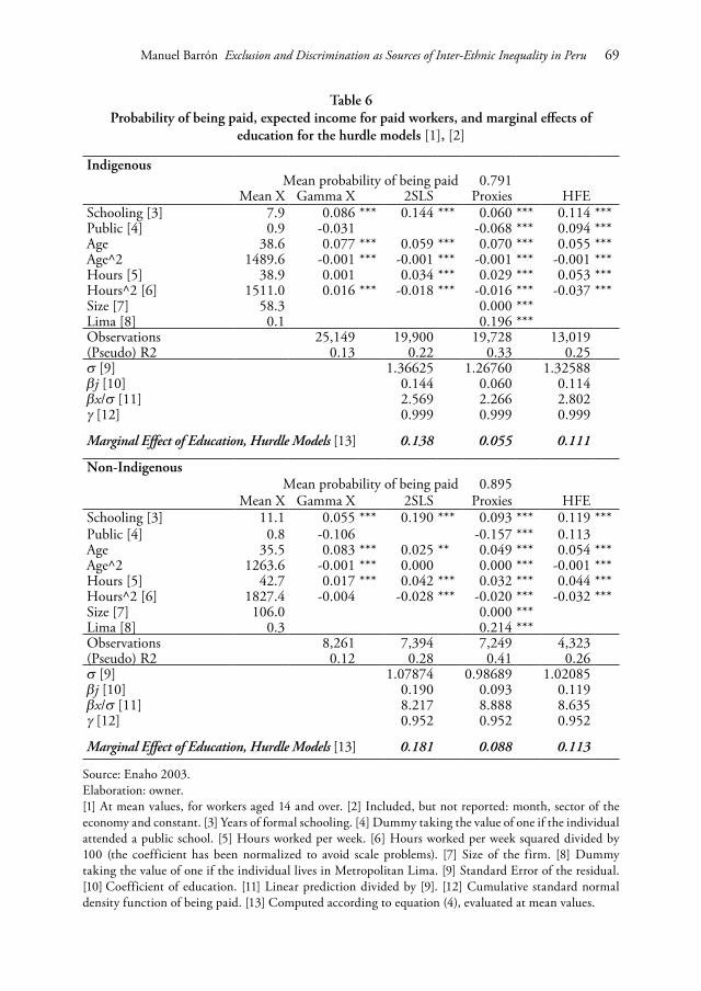
Table6Probabilityofbeingpaid,expectedincomeforpaidworkers,andmarginaleffectsof

educationforthehurdlemodels[1],[2]

IndigenousMean probability of being paid 0.791

Mean X Gamma X 2SLS Proxies HFESchooling [3] 7.9 0.086 *** 0.144 *** 0.060 *** 0.114 ***Public [4] 0.9 -0.031 -0.068 *** 0.094 ***Age 38.6 0.077 *** 0.059 *** 0.070 *** 0.055 ***Age^2 1489.6 -0.001 *** -0.001 *** -0.001 *** -0.001 ***Hours [5] 38.9 0.001 0.034 *** 0.029 *** 0.053 ***Hours^2 [6] 1511.0 0.016 *** -0.018 *** -0.016 *** -0.037 ***Size [7] 58.3 0.000 ***Lima [8] 0.1 0.196 ***observations 25,149 19,900 19,728 13,019(Pseudo) R2 0.13 0.22 0.33 0.25σ [9] 1.36625 1.26760 1.32588βj [10] 0.144 0.060 0.114βx/σ [11] 2.569 2.266 2.802γ [12] 0.999 0.999 0.999

Marginal Effect of Education, Hurdle Models [13] 0.138 0.055 0.111

Non-IndigenousMean probability of being paid 0.895

Mean X Gamma X 2SLS Proxies HFESchooling [3] 11.1 0.055 *** 0.190 *** 0.093 *** 0.119 ***Public [4] 0.8 -0.106 -0.157 *** 0.113Age 35.5 0.083 *** 0.025 ** 0.049 *** 0.054 ***Age^2 1263.6 -0.001 *** 0.000 0.000 *** -0.001 ***Hours [5] 42.7 0.017 *** 0.042 *** 0.032 *** 0.044 ***Hours^2 [6] 1827.4 -0.004 -0.028 *** -0.020 *** -0.032 ***Size [7] 106.0 0.000 ***Lima [8] 0.3 0.214 ***observations 8,261 7,394 7,249 4,323(Pseudo) R2 0.12 0.28 0.41 0.26σ [9] 1.07874 0.98689 1.02085βj [10] 0.190 0.093 0.119βx/σ [11] 8.217 8.888 8.635γ [12] 0.952 0.952 0.952

Marginal Effect of Education, Hurdle Models [13] 0.181 0.088 0.113

Source: Enaho 2003. Elaboration: owner.[1] At mean values, for workers aged 14 and over. [2] Included, but not reported: month, sector of the economy and constant. [3] Years of formal schooling. [4] Dummy taking the value of one if the individual attended a public school. [5] Hours worked per week. [6] Hours worked per week squared divided by 100 (the coefficient has been normalized to avoid scale problems). [7] Size of the firm. [8] Dummy taking the value of one if the individual lives in Metropolitan Lima. [9] Standard Error of the residual. [10] Coefficient of education. [11] Linear prediction divided by [9]. [12] Cumulative standard normal density function of being paid. [13] Computed according to equation (4), evaluated at mean values.


Figure 3A. Returns to Education, H2SLS

0.00

0.04

0.08

0.12

0.16

0.20

1 2 3 4 5 6 7 8 9 10 11 12 13 14 15 16 17 18schooling

retu

rns t

o ed

ucat

ion

Non IndigenousIndigenous

Figure 3B. Returns to Education, HProxies

0.00

0.04

0.08

0.12

0.16

0.20

1 2 3 4 5 6 7 8 9 10 11 12 13 14 15 16 17 18schooling

retu

rns t

o ed

ucat

ion


Figure 3C. Returns to Education, HFE

0.00

0.04

0.08

0.12

0.16

0.20

1 2 3 4 5 6 7 8 9 10 11 12 13 14 15 16 17 18schooling

retu

rns t

o ed

ucat

ion




Since hurdle models are non-linear, the information provided by Table 6 is not enough to draw strong conclusions. To get a better picture, the marginal effects of education at each year of schooling were obtained (holding the other variables at their mean values). The results are shown in Figure 3A to 3C. one must have in mind that the results will change for every change in the explanatory variables. Any other the calculations can be made with the coefficients in Table 6 and equations 4 and 5.

H2SLS and HProxies show a slightly narrowing gap in the returns to education by ethnic groups, whereas HFE shows a gap that shrinks significantly with an increase in education. According to HFE, education is equalising especially after high school.

As expected, in every case non-indigenous show higher returns to education than indigenous. However, the differences are particularly low for the basic Mincerian specification as well as for the HFE.10 Which are the «true» returns to education? The last three models are likely to be closest because they assess non-normality of the residual and endogeneity bias. However, the way endogeneity bias is assessed seems to play a central role in the determination of returns to education.

According to previous arguments, HFE seems to be the weakest methodology in this sense. Ability may vary widely between spouses; the children’s ability is likely to be a function of their parents, but not the same, thus HFE seems to be the weakest methodology. As discussed before, HProxies will tend to underestimate the effects of education but there is no strong prior that the biases will differ between groups. Since «public» seems to be a valid and informative instrument, H2SLS will be treated as the best model. It is worth noticing that HProxies and H2SLS predict similar differences in the returns to education between ethnic groups, of 3.3% and 4.3%, respectively.

8. SIMULATIoN: EFFECTS oF EXCLUSIoN AND DISCRIMINATIoN oN INEQUALITY

In this section exclusion and discrimination will be eliminated by performing simulations with the coefficients from the hurdle models, and inequality will be estimated in each case. This can be understood only as an initial approach to compare the effects of exclusion and discrimination. In a first simulation, income will be estimated for indigenous, with the estimated returns of the non-indigenous. This will give an idea of what would inequality look like if both groups had the same returns to each variable.

The second simulation tries to answer what would inequality look like if there was no exclusion. This exercise might be more difficult to understand, and has not been assessed previously. Without exclusion, indigenous people would tend to have the

10 The lower gap in the Mincerian specification is reasonable, because it drops the null incomes (that represent a higher percentage of the indigenous labour force than of the non-indigenous labour force), thus leading to the underestimation of the income gaps.


same values in the determinants of income as the non-indigenous people, i.e. the same distribution of explanatory variables. For instance, since the indigenous are excluded from the education process, they don’t have access to education to the same degree as the non-indigenous. If both groups had the same degree of access to education as the non-indigenous, they would tend to have the same distribution of years education. The same applies to the other determinants of income. Hence, without exclusion, indigenous and non-indigenous people would tend to have similar values of the explanatory variables. Following this line of argument, an «exclusion-free» income distribution was simulated using the explanatory variables for the non-indigenous with the returns obtained for the indigenous population for each hurdle model. This gives a smaller sample size for the indigenous population, because in the EAP the ratio of indigenous to non-indigenous is close to 3:1. In order to get a sample size similar to the indigenous population, each of these observations was three-folded.11 This new series and the observed income for the non-indigenous constitute the «exclusion free» income distribution. The resulting inequality is labelled «exclusion-free» inequality. The same exercise was repeated for each hurdle model.

To assess the mass of null incomes, individuals with a probability of less than 60% of having a positive income are assigned a null income. Using 50% and 70% as thresholds leaves the main results unaffected.

The results are shown in Table 7. The Gini index for the sample is 0.64. If both groups had the same returns to the determinants of income, the Gini index would decrease to 0.51 in average. If, having different returns, both groups had the same distribution of variables (i.e., with no exclusion), Gini index would be reduced even more, to 0.46. This shows that exclusion seems to play even a bigger role than discrimination in explaining inequality than the income gap.

Table7Simulationsofincomeinequalityindices

Inequalitymeasures IncomeH2SLS HProxies HFE

nodisc noexcl nodisc noexcl nodisc noexcl

Relative mean deviation 0.47 0.38 0.31 0.37 0.32 0.35 0.33Gini coefficient 0.64 0.52 0.44 0.51 0.46 0.50 0.48Theil entropy measure 0.82 0.53 0.40 0.53 0.41 0.54 0.51Theil mean log deviation measure 0.43 0.41 0.22 0.38 0.24 0.34 0.24


11 This is not completely accurate, because the survey has a complex stratification structure, and weights vary along the population, but that is not being assessed. Thus, this must be seen as a rough approximation only.


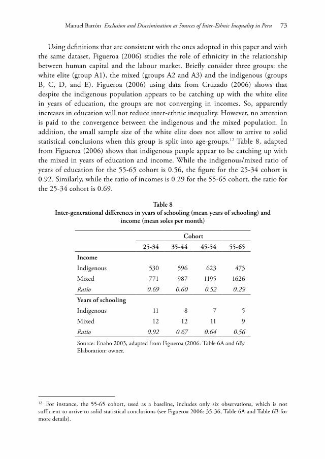
Using definitions that are consistent with the ones adopted in this paper and with the same dataset, Figueroa (2006) studies the role of ethnicity in the relationship between human capital and the labour market. Briefly consider three groups: the white elite (group A1), the mixed (groups A2 and A3) and the indigenous (groups B, C, D, and E). Figueroa (2006) using data from Cruzado (2006) shows that despite the indigenous population appears to be catching up with the white elite in years of education, the groups are not converging in incomes. So, apparently increases in education will not reduce inter-ethnic inequality. However, no attention is paid to the convergence between the indigenous and the mixed population. In addition, the small sample size of the white elite does not allow to arrive to solid statistical conclusions when this group is split into age-groups.12 Table 8, adapted from Figueroa (2006) shows that indigenous people appear to be catching up with the mixed in years of education and income. While the indigenous/mixed ratio of years of education for the 55-65 cohort is 0.56, the figure for the 25-34 cohort is 0.92. Similarly, while the ratio of incomes is 0.29 for the 55-65 cohort, the ratio for the 25-34 cohort is 0.69.

Table8Inter-generationaldifferencesinyearsofschooling(meanyearsofschooling)and

income(meansolespermonth)

Cohort

25-34 35-44 45-54 55-65

Income

Indigenous 530 596 623 473Mixed 771 987 1195 1626Ratio 0.69 0.60 0.52 0.29

Yearsofschooling

Indigenous 11 8 7 5Mixed 12 12 11 9Ratio 0.92 0.67 0.64 0.56

Source: Enaho 2003, adapted from Figueroa (2006: Table 6A and 6B).Elaboration: owner.

12 For instance, the 55-65 cohort, used as a baseline, includes only six observations, which is not sufficient to arrive to solid statistical conclusions (see Figueroa 2006: 35-36, Table 6A and Table 6B for more details).


Since education seems to play at least a partial role in reducing inequality, some policy experiments will be sketched to illustrate the relevance of the results presented in section 7. Their effects on inequality are presented in Table 9:13

1. Policy 1: Increase one year of schooling for the indigenous people who didn’t finish high school.

2. Policy 2: Increase three years of schooling for the indigenous people who didn’t finish high school, or guarantee they finish high school, whatever is lower.

3. Policy 3: Increase five years of schooling for the indigenous people who didn’t finish high school, or guarantee they finish high school, whatever is lower.

4. Policy 4: Guarantee that all indigenous who finish high school also finish technical studies (two years after high school).

Table9Policysimulations,H2SLSmodel

StatusQuo POL1 POL2 POL3 POL4

Relative mean deviation 0.47 0.39 0.38 0.39 0.37Gini coefficient 0.64 0.54 0.54 0.55 0.51Theil entropy measure 0.82 0.62 0.62 0.62 0.54Theil mean log deviation measure 0.43 0.24 0.24 0.25 0.40


Policy 1 can be interpreted as a short term policy, Policy 2 as a medium term, and Policy 3 as long term. They would benefit around 70% of the indigenous population (Table 1). These three policies would have similar effects on income inequality. An increase of one year has a similar effect as an increase in three or five years, because the ethnic gap is high and roughly constant at the first stages of education (figures 3A to 3C). However, this does not imply that education should be increased in one year only, for education is a human right, an end in itself. It increases human liberties and capabilities (Sen 1999) and fosters political citizenship (Ames 1978). Therefore, the evaluation of the returns to education based just on the effect of education on income consists in an underestimation of the true effects.

Policy 4 shows that post high school studies have a stronger impact on income distribution. Except for Theil’s second measure, Policy 4 implies the highest reduction in inequality. Policy 4 basically guarantees technical education to all the indigenous high school graduates. Despite this policy would benefit only 30% of the indigenous population, its effects on inequality are higher, because the inter-ethnic income gap is

13 For the sake of space, only the results for the H2SLS model are presented, but the other models are consistent.


lower at the higher levels of education (figures 3A to 3C). In addition, this policy would also give incentives to parents to send their children to school, knowing that after that the State would guarantee superior studies, and therefore higher incomes.

Targeting issues arise. Positive discrimination can also be dangerous. Being non-indigenous does not mean being educated or non-poor. Many non-indigenous people also need assistance from the State, and they cannot be left aside.

Does the State have incentives to pursue these policies? If the State maximises votes, it lacks incentives to expand education. In the short term, it is more politically profitable to give «gifts» than «rights» (Figueroa 2003). While the former consist of basic social assistance, food, and clothing, the latter include education, healthcare and political citizenship.

The success of the policies illustrated here requires not only the supply of education, construction of schools, and hiring of more teachers; demand might also require incentives: e.g. to offer breakfast at school, free uniforms, books.

Endless policies can be simulated. For example, these models could be used to assess the effects of universalising primary schooling (attributing six years of schooling to anyone who has less than that). Policies not necessarily related to education can also be assessed, as promoting migration to the capital or giving incentives to employers to hire formal employment (which would also lessen the uncertainty effects of being self-employed).

9. CoNCLUSIoNS AND PoLICY IMPLICATIoNS

Between-group inequality contributes to almost 10% of overall inequality; and that is reflected on important differences in average income between indigenous and non-indigenous. Mean income for the non-indigenous people is twice than that for the indigenous. Moreover, expected lifetime income for an average indigenous worker is just 44% of the figure for the average non-indigenous worker.

The econometric analysis in section 7.2 has shown that education has positive effects on income, with diminishing marginal effects at each year of schooling. Age and hours worked also show positive but decreasing marginal returns. The difference in the distribution of years of schooling seems to be one of the most important sources of inequality, so reducing the gap in years of schooling would reduce inter-ethnic inequality in a significant way. Despite public education is regarded as low-quality, promoting it would have positive effects on income. This does not mean that quality does not matter, but that, being income inequality so severe, any improvement will help. However, other policies should be directed to tackle down the problems outlined by Figueroa (2006:11-17).

The literature focuses on the differences in the slopes of the regression lines (discrimination), but usually neglects the importance of the distribution of the


regressors (exclusion). Trivelli (2005) is a notable exception in this respect, but her methodology leaves aside the population with null incomes and therefore her results are arguably biased. Addressing the problems of econometric endogeneity of education and of truncation-at-zero of the income distribution, this paper has shown that exclusion explains a larger share of income inequality than discrimination. According to the simulations performed in section 8, without discrimination income inequality (measured by the Gini index) would be reduced by 20%, and without exclusion, by 28%. Hence, despite most quantitative research on Peru’s interethnic income gap has focused on discrimination, exclusion seems to be a more important source of inequality, and therefore more important to tackle down.

Partial reductions of exclusion in the access to education would reduce inequality as much as the complete elimination of discrimination. Four policies are proposed as illustrations in section 8, and it is found that increases of one or two years of schooling can reduce income inequality (as measured by the Gini) by as much as 15% to 20%, depending on whether the change is in the lower or the upper tails of the distribution of years of education.

Policies directed to tackle down exclusion tend to be expensive, both politically and economically. As Figueroa (2003) argues, no agent has the incentives and the resources to change the observed outcome. The government lacks incentives to destine resources to the inclusion of excluded populations, because giving gifts is politically more profitable than granting rights. As Barrón (forthcoming) shows, this does not seem to be a problem of economies of scale either. The agent with both incentives and power to implement these policies has not been identified in this paper, which constitutes a serious caveat.

The changes in inequality presented here should be taken as lower limits to the actual changes. Externalities to lower exclusion or discrimination would transform the whole economy: with a better educated labour force, investment in industries that demand qualified labour would be profitable, and it is well known that these industries drive up wages, with further effects on poverty and inequality. In second place, in a more stable country, financial markets can be developed more easily, and therefore credit and insurance would be expanded. Although the latter would not reach the poor directly (especially not the rural poor), they might be reached indirectly, through social networks.14

14 The effects are highly complex. For thorough reviews of these mechanisms, see Dercon (2004) and Fafchamps (2003).


REFERENCES

Acemoglu, Daron, Simon Johnson and James Robinson 2002 «Reversal of Fortune: Geography and Institutions in the Making of the Modern World

Income Distribution». TheQuarterlyJournalofEconomics, Vol. 117, N° 4, pp. 1231-1294, Cambridge, MA.

Albó, Xavier 2002 PueblosIndiosenlapolítica.Cuadernos de Investigación CIPCA, N° 59. La Paz: Centro

de Investigación y Promoción del Campesinado, Plural.

Albó, Xavier and Víctor Quispe2004 ¿Quiénessonindígenasenlosgobiernosmunicipales? Cuadernos de Investigación CIPCA,

N° 55. La Paz: Centro de Investigación y Promoción del Campesinado, Plural.

Ames, Rolando (editor) 1978 SituaciónyderechospolíticosdelanalfabetoenelPerú. Lima: Pontificia Universidad Católica

del Perú.

Anand, Sudhir 1983 Inequality and Poverty in Malaysia: Measurement and Decomposition. oxford: oxford

University Press.

Aslam, Monazza and Geeta Kingdon2005 Gender and Household Expenditure in Education in Pakistan. Global Poverty Research

Group Working Paper N° 25. oxford: University of oxford.

Assies, Willem, Gemma van der Haar and André Hoekema2000 TheChallengeofDiversity: IndigenousPeoplesandReformof theState inLatinAmerica.

Amsterdam: Thela - Thesis.

Barrón, Manuel 2005 «¿Cuánto cuesta ser provinciano a un empleado en Lima Metropolitana?: Una aproximación

mediante PropensityScoreMatching». ObservatoriodelaEconomíaLatinoamericana, N° 47. Available at: <www.eumed.net/cursecon/ecolat/>

N.d. HorizontalInequalitiesinLatinAmerica:AStatisticalComparisonofBolivia,GuatemalaandPeru. CRISE Working Paper. oxford: University of oxford (forthcoming).

Cameron, Colin and Pravin Trivedi 1998 RegressionAnalysisofCountData. New York: Cambridge University Press.

Case, Anne and Angus Deaton 1999 «School Inputs and Educational outcomes in South Africa». The Quarterly Journal of

Economics, Vol. 114, N° 3, pp. 1047-1084, Cambridge, MA.

Cruzado, Viviana 2006 Informe de investigación: educación y mercados laborales en la sociedad sigma. Estudio

del caso peruano para los años 2002 y 2003. Lima: Departamento de Economía, Pontificia Universidad Católica del Perú (mimeo).


Deininger, Klaus and Lyn Squire1996 «A New Dataset Measuring Income Inequality». TheWorldBankEconomicReview, Vol.

10, N° 3, pp. 565-591, Washington, D.C.

Dercon, Stefan 2004 InsuranceagainstPoverty. oxford: oxford University Press.

Diamond, Jared 1997 Gus,Germs,andSteel:TheFateofHumanSocieties. New York: W. W. Norton and Co.

Engerman, Stanley and Kenneth Sokoloff2002 «Inequality Before and After the Law: Paths of Long-Run Development in the Americas».

Paper presented at the Annual Bank Conference on Development Economics Europe, in oslo, Norway, between June 24-26.

Estela Benavides, Manuel2001 Perú:Ocho apuntes para el crecimiento con bienestar. Lima: Fondo Editorial del Banco

Central de Reserva del Perú.

Fafchamps, Marcel 2003 RuralPoverty,RiskandDevelopment. Cheltenham: Edward Elgar.

Figueroa, Adolfo 2002 Economic Elites and Social Capital. CISEPA Working Paper N° 214. Lima: Pontificia

Universidad Católica del Perú.2003 La sociedad sigma: Una teoría del desarrollo económico. Lima and Mexico D.F.: Fondo

Editorial de la Pontificia Universidad Católica del Perú and Fondo de Cultura Económica.

2006 Elproblemadel empleo enuna sociedad sigma. CISEPA Working Paper N° 249. Lima: Pontificia Universidad Católica del Perú.

Figueroa, Adolfo, Teófilo Altamirano and Dennis Sulmont1996 SocialExclusionandInequalityinPeru. ILo Research Series N° 104. Geneva: International

Institute for Labour Studies.

Figueroa, Adolfo and Manuel Barrón2005 Inequality,EthnicityandSocialDisorderinPeru. CRISE Working Paper8. oxford: Centre

for Research on Inequality, Human Security and Ethnicity, University of oxford.

Glewwe, Paul 2002 «Schools and Skills in Developing Countries: Education Policies and Socioeconomic

outcomes». JournalofEconomicLiterature, Vol. 40, N° 2, pp. 436-482, Cambridge.

Hanushek, Erick and Javier Luque2003 «Efficiency and Equity in Schools Around the World». Economicsof EducationReview,

Vol. 22, N° 2, pp. 131-141, Cambridge, MA.

Haya de la Torre, Víctor Raúl 1984 [1923] «Aspectos del Problema Social en el Perú». In Luis Alberto Sánchez etal. (editors).

VíctorRaúlHayadelatorre:Obrascompletas. Vol. 1, 3rd edition. Lima: Editorial Juan Mejía Baca.


Instituto Nacional de Estadística e Informática (INEI) 2004 Fichatécnica-Enaho2003.

Krueger, Alan1999 «Experimental Estimates of Education Production Functions». TheQuarterlyJournalof

Economics, Vol. 114, N° 2, Cambridge, MA.

Li, Hongyi, Lyn Squire and Heng-Fu Zou1997 «Explaining international and intertemporal variations in income inequality». The

EconomicJournal, Vol. 108, N° 446, pp. 26-43, London.

Mac Isaac, Donna1994 «Peru». In George Psacharopoulos and Harry Patrinos (editors). IndigenousPeopleand

PovertyinLatinAmerica:AnEmpiricalAnalysis. Washington, D.C.: The World Bank, pp. 165-204.

Mahoney, James2003 «Long-Run Development ant the Legacy of Colonialism in Spanish America». American

JournalofSociology, Vol. 109, N° 1, pp. 50-106, Chicago.

Mariátegui, José Carlos1968 [1928] Sieteensayosdeinterpretacióndelarealidadperuana. 13th edition. Lima: Biblioteca

Amauta.

Moreno, Martín, Hugo Ñopo, Jaime Saavedra and Máximo Torero2004 Gender and Racial Discrimination in Hiring: A Pseudo-Audit Study of Three Selected

Occupations in Metropolitan Lima. IZA Discussions Papers N° 979. Bonn, Germany: Institute for the Study of Labor.

Mullahy, John 1986 «Specification and Testing of Some Modified Count Data Models». JournalofEconometrics

Vol. 33, N° 3, pp. 341-365, Amsterdam.

Ñopo, Hugo 2004 Matching as a tool to DecomposeWage Gaps. IZA Discussion Papers N° 981. Bonn,

Germany: Institute for the Study of Labor.

Ñopo, Hugo, Jaime Saavedra and Máximo Torero2004 Ethnicity and Earnings in Urban Peru. IZA Discussion Papers 980. Bonn, Germany:

Institute for the Study of Labor.

Sen, Amartya 1999 DevelopmentasFreedom. oxford: oxford University Press.

Todd, Petra and Kenneth Wolpin2003 «on The Specification and Estimation of The Production Function for Cognitive

Achievement». TheEconomicJournal, Vol.113, N° 485, pp. 3-33, London.

Torero, Máximo, Jaime Saavedra, Hugo Ñopo, and Javier Escobal2004 «The Economics of Social Exclusion in Peru: An Invisible Wall?». In Mayra Buvinic,

Jacqueline Mazza and Ruthanne Deutsch (editors). Social Inclusion and EconomicDevelopmentinLatinAmerica. Washington, D.C.:Johns Hopkins University Press and Inter-American Development Bank, pp. 221-246.


Trivelli, Carolina 2005 Los hogares indígenas y la pobreza en el Perú: una mirada a partir de la información

cuantitativa. Instituto de Estudios Peruanos Working Paper N° 141. Lima: Instituto de Estudios Peruanos.

Wooldridge, Jeffrey2002 EconometricAnalysisofCross-SectionandPanelData. Cambridge, MA and London: The

MIT Press.

exclusion and discrimination as sources of inter …manuelb/research/exclusion and... · manuel...

Documents