means-testing and tax rates on earnings - …saez/brewer-saez-shephardmr10book.pdf · cutting child...
TRANSCRIPT

2
Means-testing and Tax Rates on Earnings
Mike Brewer, Emmanuel Saez, and Andrew Shephard∗
Mike Brewer is Director of the Direct Tax and Welfare ResearchProgramme at the IFS and a Research Affiliate of the National PovertyCenter at the University of Michigan. His main research interests are inthe impact of welfare reform and the personal tax and benefit system onfamilies with children. He has evaluated the labour market impact of theworking families’ tax credit, and the impact of a time-limited in-workprogramme for lone parents in the UK. He has written widely about thecurrent UK government’s ambition to eradicate child poverty.
Emmanuel Saez is a Professor of Economics at the University ofCalifornia, Berkeley, and a Research Associate at the National Bureauof Economic Research. He received his PhD in Economics from MITin 1999. He is currently Editor of the Journal of Public Economics. Hismain areas of research are taxation, redistribution, and income andwealth inequality. In the field of optimal income taxation, he has notablypublished ‘Using Elasticities to Derive Optimal Income Tax Rates’ in theReview of Economic Studies and ‘Optimal Income Transfer Programs’ inthe Quarterly Journal of Economics.
Andrew Shephard is a PhD scholar at the IFS, where he was previously aResearch Economist. His main research interests are in structural modelsof the labour market, the application of these models in evaluating policyreforms, and the implication of these models for tax design.
∗ We thank Stuart Adam, Tony Atkinson, Kate Bell, Richard Blundell, Hilary Hoynes, Paul John-son, Guy Laroque, Costas Meghir, James Mirrlees, Robert Moffitt, James Poterba, and numerousconference participants for helpful comments and discussions. Saez acknowledges financial supportfrom the National Science Foundation grant SES-0134946. The Survey of Personal Incomes, theLabour Force Survey, and Family Expenditure Survey, the Family Resources Survey and the GeneralHousehold Survey datasets are crown copyright material, and are reproduced with the permissionof the Controller of HMSO and the Queen’s Printer for Scotland. The SPI, LFS, and GHS datasetswere obtained from the UK Data Archive, FRS from the Department for Work and Pensions, andthe FES from the Office for National Statistics. None of these government departments nor the UKData Archive bears any responsibility for their further analysis or interpretation.

Means-testing and Tax Rates on Earnings 91
EXECUTIVE SUMMARY
The setting of income tax rates and the generosity and structure of incomesupport programmes generate substantial controversy among policy-makersand economists. At the centre is a trade-off between the goals of equityand efficiency: governments want to transfer resources from the rich tothe poor; on the other hand, such transfers reduce people’s incentive towork.
The key insight from the standard ‘optimal income tax model’ developedby James Mirrlees is that marginal rates of tax and benefit withdrawal shouldbe higher when people’s choices of how much to work are relatively unre-sponsive to them and when the government is relatively keen to redistributeresources from rich to poor. Furthermore, the government should apply highmarginal rates at points in the earnings distribution where there are fewtaxpayers relative to the number of taxpayers who have earnings exceedingthis amount. Using data on the UK earnings distribution, we show that theoptimal structure of marginal rates in this simplified model has a U-shapedpattern, with high marginal rates imposed on high and low earners and lowermarginal rates on those in the middle. We show how this structure changesas both the assumed responsiveness of hours of work and the government’sassumed preferences for redistribution vary.
The way that incomes have responded to the large changes in top marginaltax rates over the past forty years suggests that if the richest 1% see a 1% fall inthe proportion of each additional pound of earnings that is left after tax, thenthe income they report will rise by less than half that—only 0.46%. Althougha tentative estimate, this suggests that the government would maximize therevenue it collects by imposing an overall marginal rate on the highest earnersof 56.6%, very close to the 52.7% currently charged in the UK (includingincome tax, National Insurance contributions, and indirect taxes). So theredoes not seem a powerful case for increasing the income tax rate on the veryhighest earners, even on redistributive grounds—it would not generate much,if any, extra revenue to transfer to the less well off.
When the optimal tax model is enriched by allowing individuals to respondto taxes and benefits by deciding whether or not to work, as well as howhard, then the optimal structure of marginal rates changes dramatically.In particular, when the decision whether to work becomes relatively moreimportant than the decision about how much to work, then marginal ratesand the proportion of gross income taken in tax and withdrawn benefitswhen people enter work should be set low (and perhaps even negative) forpotential low earners rather than set high as the standard model suggests.

92 Mike Brewer, Emmanuel Saez, and Andrew Shephard
We also discuss how the design of taxes and benefits affecting an individualshould be affected by the presence of a co-resident partner or dependentchildren, although it is difficult to reach definitive conclusions. We argue thatthe practical operation of benefits and tax credits for low-income familiesis important and that they would be of greatest help to beneficiaries if theywere assessed over short periods and paid promptly without retrospectiveadjustment.
These insights from optimal tax theory are contrasted with the work incen-tives inherent in the current UK tax and benefit system. Four key deficienciesare identified:
1. The amount of gross income taken in tax and withdrawn benefits whenpeople enter work at low earnings is too high: for most groups it is closeto 100% before individuals are entitled to the working tax credit, andthey remain high even with it.
2. The marginal rate of 73.4% that many low to moderate earners facewhen having tax credits withdrawn is likely to be above the opti-mal rate even if people’s decision to work a little harder is relativelyunresponsive.
3. Housing Benefit, the main means-tested programme through which thegovernment helps people on relatively low incomes with their housingcosts has an extremely high withdrawal rate. This exacerbates the prob-lem of undesirably high marginal rates. It is also hard to administer andis not claimed by many working families entitled to it.
4. While the system for administering income tax and national insurancecontributions in the UK is simple and efficient, tax credits, housingbenefit, and council tax benefit are all burdensome to claim, relativelyexpensive for the government to administer, and prone to significantfraud and error.
Given this diagnosis, we suggest a set of changes to the existing tax andbenefit structure that could be made immediately based on the lessons fromour analysis. Our package of ‘immediate reforms’ involves:
� Increasing the amount people can earn before they have means-testedbenefits withdrawn. This would increase the financial gain on enteringwork at low earnings.
� Increasing the amount that second earners can earn before a family’s taxcredits are withdrawn. This would improve the financial incentive for asecond earner to enter work, especially if they have children.

Means-testing and Tax Rates on Earnings 93
� Reducing the rate at which child and working tax credits are withdrawnwith every extra pound earned.
� Targeting increases in working tax credit on groups other than loneparents.
This would cost around £9 billion per year. If it had to be financed fromwithin the income tax and benefit system, the money could be raised bycutting child benefit and/or increasing the basic rate of income tax. Neitherwould undo the objectives of the reform package to improve work incentives,although both would pose big political challenges.
We also suggest a more radical and comprehensive plan for reforming theUK household tax and benefit system that attempts to deal not only with thesework incentive issues, but also the administrative failings that we identify.Our plan replaces the existing piecemeal benefits for low-income families(income support, working and child tax credits, housing benefit, and counciltax benefit) with a single Integrated Family Support (IFS) programme whichprovides stronger and simpler incentives for work at the bottom, reducescompliance costs for families, and is means-tested by employers’ withholdingfrom earnings in the same way as for National Insurance contributions. Weshow how, after including an assessment of the behavioural responses, the IFSmanages to redistribute more income with minimal impact on total earningsand total net tax revenue, by targeting net tax cuts where incentives to workare currently at their weakest.
2.1. INTRODUCTION
The setting of income tax rates, and the generosity and structure of incomesupport (or transfer) programmes generate substantial controversy amongpolicy-makers and economists. At the centre is an equity–efficiency trade-off. On the one hand, governments value redistribution, and so want totransfer resources from the rich to the poor, usually by taxing the incomesof the rich and subsidizing the incomes of the poor. On the other hand, thisredistribution is generally costly in terms of economic efficiency because ofthe disincentive effects of taxes and transfers (we explain this in more detailin Section 2.2). The costs arise for two reasons: first, raising income taxesmay weaken the labour supply and entrepreneurship incentives of middle-and high-income individuals who face the taxes. Second, income transferprogrammes may weaken the labour supply incentives of their recipients.

94 Mike Brewer, Emmanuel Saez, and Andrew Shephard
These two responses can substantially raise the cost of improving the livingstandards of low income families.
The goal of this chapter is to provide an overview of the way economiststhink about the design of taxes and benefits affecting households, and toapply the lessons from this literature to the design of the UK tax and benefitsystem.
In economics research, the problem of designing taxes and benefits istackled in two steps. The first step is a positive analysis, where economistsdevelop models of individual behaviour to understand how individuals’ workdecisions respond to taxes and benefits. The central part of the positiveanalysis is the empirical estimation of models of individual behaviour, andthere is a very broad literature that tries to estimate the size of the behaviouralresponses to taxes and benefits.1
The second step is the normative analysis, or optimal policy analysis. Usingmodels developed in the positive analysis, the normative analysis investigateswhat structure and size of the tax and benefit system would best meet a givenset of policy goals; following Mirrlees (1971), economists call this line ofresearch ‘optimal tax theory’. Despite its name, optimal tax theory concernsitself just as much with the design of benefits as it does the setting of incometax rates: one of the key concepts of optimal tax theory is that of a nettax function, whereby people with high incomes pay some of that incomein positive taxes to the government, and people with a low income receivemoney from the government (by paying negative taxes); no conceptual dis-tinction is made between net recipients from and net contributors to thestate’s finances.2
At its heart, optimal tax theory says that the two desirable features of atax and benefit system are that it be fair, and that it minimize disincentiveeffects.3 But the problem of having two desirable features is that one has toknow how much weight to give to each. For example, a poll tax (under whichall individuals have to pay the same level of tax) might have no disincentiveeffects, but is rather unfair to those on low incomes. As Heady (1993, p. 17)says, ‘the approach of the optimal tax literature is to use economic analysisto combine these criteria into one’. It does this by saying that the objective
1 The way that these models are estimated, and the key insights, are summarized in Meghir andPhillips, Chapter 3.
2 One difference between the tax system and the transfer system is that the former is usuallycheaper to administer, and these distinctions can be reflected in more complicated optimal taxmodels.
3 More complicated models can allow for other desirable features: one might be that a tax andtransfer system is cheap to administer; Shaw, Slemrod, and Whiting, Chapter 12, consider how thisalters optimal tax models.

Means-testing and Tax Rates on Earnings 95
of the government when designing the tax and benefit system should beto maximize social welfare (subject to a need to raise a certain amount ofrevenue). Precisely how social welfare is expressed is not relevant at thisstage, but the idea is that it reflects in a single index (or number) the desireboth to have the economy as large as possible (because this directly increasespeople’s well-being) but also to have the income distributed as equally aspossible. The expression for social welfare precisely quantifies the trade-off between these two desiderata: returning to the previous example of aneconomy with only a poll tax, replacing that with an income tax whichraised the same amount of money would give a more equal distributionof income, but—if there are any disincentive effects to taxation—a smallereconomy.
The normative analysis is crucial for policy-making because it shows howtaxes and benefits should be designed in order best to attain the goals ofthe policy-maker. In particular, the normative analysis allows one to assessseparately how changes in the redistributive criterion of the government,and changes in the size of the behavioural responses to taxes and transfers,affect the optimal tax and benefit programme. Conversely, the normativeanalysis makes it explicit that one cannot hope to say how best to designtaxes and transfers both without knowing how individuals will respond, andwithout specifying what one is trying to achieve overall. Often, these twoelements are confused in policy debates: right-of-centre policy-makers rarelystate explicitly that they have little taste for redistribution, but instead justifytheir lack of taste for redistribution because they believe that the adversebehavioural responses to high taxes or generous benefits are large. Conversely,left-of-centre policy-makers emphasize the redistributive virtues of benefitsand assume that adverse behavioural responses to these and the high tax ratesneeded to fund them are negligible.
We provide this overview as follows: Section 2.2 introduces the standardoptimal tax model developed in Mirrlees (1971). This shows directly howthe optimal tax and benefit system is determined by both the social welfarecriterion used by the government and the size of behavioural responses totaxation. Despite the simplifications inherent in the model, we can use itto analyse the optimal tax rate that should apply to top incomes, wherewe present new, albeit tentative, evidence on the response of top incomesto the large changes in top marginal tax rates that have taken place in theUK over the last forty years. Section 2.3 extends the optimal tax model toallow for labour supply participation effects, and shows that allowing forsuch responses can drastically change the optimal tax system affecting low-income individuals: instead of traditional welfare programmes with high
96 Mike Brewer, Emmanuel Saez, and Andrew Shephard
withdrawal rates, large in-work benefits such as Working Tax Credit in theUK or the Earned Income Tax Credit from the US, which can have very lowor negative withdrawal rates, can be optimal.4 We also discuss the issue ofmigration and tax design, which can be dealt with in optimal tax modelsin a similar manner to the issue of labour market participation. Through-out Sections 2.4 and 2.5, we make use of the summary of the literatureon the behavioural response to taxation provided in Meghir and Phillips,Chapter 3.
In Section 2.4, we discuss how the family should be taxed: the modelsconsidered in Sections 2.2 and 2.3 abstract from family issues, but a majorityof adults in reality live in couples, and so can be assumed to pool incometo some extent. We also discuss how the presence of children should bereflected in the optimal tax design. Section 2.5 discusses conditionality, thecontributory principle and administrative and operational issues concerningbenefit systems.5 Section 2.6 describes how the main elements of the currentUK personal tax and benefit system affect incentives to work and earn moreand, in Section 2.7, we provide a critique of the UK tax and benefit system,and set out the direction of reform suggested by the insights from optimal taxtheory, and the latest evidence on the behavioural response to taxation. Tocrystallize ideas, we propose specific changes that could be implemented inthe short run. But most optimal tax theory uses simplified models which leaveaside a number of important practical issues such as administrative burdenfor the government and employers, and ease of use for families.6 Those issueshave always been important in practice, and the recent ‘behavioural eco-nomics’ literature is starting to incorporate them in the analysis. Therefore,we go further and propose a longer-term reform that builds on the short-runchanges to incentives by addressing the main practical issues with the currentbenefits in the UK. Our plan replaces the piecemeal benefits for low-incomefamilies (income support, working and child tax credits, housing benefit, andcouncil tax benefit) into a single Integrated Family Support programme whichprovides stronger and simpler incentives for work at the bottom, reducescompliance costs for families, and is provided ‘as-you-earn’ and administeredin the same way as social contributions through the PAYE withholding sys-tem.We show how this can be done in a revenue-neutral fashion, and estimatethe behavioural responses to such a reform.
4 To anticipate our discussion in Section 2.5, the WTC can lead to negative PTRs, but not negativeMETRs, whereas the EITC can lead to negative METRs as well.
5 Shaw, Slemrod, and Whiting, Chapter 12, discuss administrative and operational issues affect-ing tax design.
6 A number of those issues are discussed in more detail in Chapter 12 by Shaw, Slemrod, andWhiting.

Means-testing and Tax Rates on Earnings 97
2.2. THE STANDARD OPTIMAL INCOME TAX MODELWITH INTENSIVE RESPONSES
This section presents the standard model of optimal income tax, based onMirrlees (1971), in which individuals respond to the tax and benefit systemby choosing only how much to work. We then give two applications of themodel to the UK:
� First, we can derive an expression for the optimal top marginal tax rate(i.e., the marginal tax rate facing the highest income individuals), andwe go on to calculate this using new, albeit tentative, evidence on theresponsiveness of top incomes in the UK to changes in top marginal taxrates over the last forty years.
� Second, we simulate the entire optimal tax system for the UK given somevarious highly simplifying assumptions in order to show how the optimaltax system is determined by both the social welfare criterion used by thegovernment, and the size of behavioural responses to taxation.
Before that, though, Section 2.2.1 sets out some of the key terms which willoccur throughout this chapter.
2.2.1. Key concepts
The budget constraint, PTRs and METRs
A useful tool to investigate the disincentive effects of taxes and transfers isthe budget constraint.7 This shows the relationship between gross earnings(or hours of work) and net income after taxes and transfers, and an exampleis given in Figure 2.1A (the example is for a lone parent with two children,and we discuss this figure in more detail and look at other family types inSection 2.6).
The budget constraint contains all the information we need to know abouthow taxes and transfers affect financial incentives to work, but in this chapterwe frequently refer to some summary measures of work incentives:
� The participation tax rate (PTR) is defined as 1 minus the financial gainto work as a proportion of gross earnings. It measures how the tax andbenefit system affects the financial gain to work. If someone who didnot work had an income from a benefit programme of £60 a week, andwould earn £250 in gross earnings, but pay £40 of that in income tax if
7 This draws on Chapter 2 of Adam et al. (2006).

98 Mike Brewer, Emmanuel Saez, and Andrew Shephard
0
10,000
20,000
30,000
40,000
50,000
60,000
Cost to employer, £/year
Net
inco
me,
£/y
ear
70,00060,00050,00040,00030,00020,00010,0000
Notes: Assumes a lone parent with two children, paying £80 per week in rent, no childcare costs, averageBand C council tax, and with a wage of £5.52 per hour. Incomes are calculated under the April 2008 taxand benefit system with announced changes to the higher-rate threshold and UEL, but without the £600rise in the income tax personal allowance.
Figure 2.1A. Example budget constraint, lone parent
they were to work, then the PTR is given by 1−(210–60)/250, or 40%.The higher the number, the more the tax and benefit system reduces thefinancial gain to work. A PTR in excess of 1 means the individual wouldbe worse off in work than not working; a PTR equal to 1 means that thereis no financial reward to work; a PTR of zero means that the financialreward to work is equal to gross earnings; negative PTRs are possi-ble where benefits are conditional on being in work or having positiveearnings.
� The marginal effective tax rate (METR) measures how much of a smallrise in gross earnings is lost to payments of tax and reduced entitle-ments to benefits. It is equal to the slope of the budget constraint at anyparticular point. The higher the number, the more the tax and benefitsystem reduces the gain to earning a bit more: a METR in excess of 1means that an individual would be worse off if they earned a bit more;a METR of 1 means that an individual would be unaffected by anysmall change in earnings; a METR of zero means that the individual iskeeping all of any small rise in earnings; and a negative METR meansthat an individual’s net income increases by more than a small change inearnings (this can arise where benefits act as a proportional subsidy on

Means-testing and Tax Rates on Earnings 99
0%0 10,000 20,000 30,000 40,000 50,000 60,000 70,000
20%
40%
60%
80%
100%
120%
Cost to employer, £/year
Par
tici
pat
ion
an
d m
arg
inal
tax
rat
e
PTR
MTR
Notes: As for Figure 2.1A.
Figure 2.1B. Participation and marginal tax rates, lone parent
earnings, such as the phase-in portion of the earned income tax credit inthe US).
� It is sometimes more useful to consider the net-of-tax rate, or one minusthe METR: this measures how much work pays at the margin.
Figure 2.1B shows the schedule of PTRs and METRs for the examplebudget constraint in Figure 2.1A; we discuss the particular features of thisbudget constraint in Section 2.6.
Labour supply responses to taxation
Economists think about the disincentive effects of the tax and benefit systemusing a labour supply model.8 A basic labour supply model assumes that,when deciding whether and how much to work, people trade off the financialreward to working (plus any intrinsic benefits from working) with the loss ofleisure time (by ‘work’ we mean ‘participate in the labour market’, rather thandoing unpaid work at home or elsewhere).
As we discussed above, taxes and transfers affect labour supply because theyalter the financial reward to working, both by making the net wage lower than
8 See Meghir and Phillips, Chapter 3, and references therein, for more detail.

100 Mike Brewer, Emmanuel Saez, and Andrew Shephard
the gross wage (most taxes, some transfers) and by reducing the financialgain from working compared to not working (most transfers). Economistsusually distinguish between two ways that financial considerations affectlabour supply:9
1. The impact of the METR on labour supply is called the substitutioneffect, as increasing the METR (thereby reducing the net-of-tax rate)may lead individuals to work less, or to substitute some leisure forwork. Economists often measure this effect using the elasticity of earn-ings with respect to the net-of-tax rate: this measures the percentageincrease in earnings following a one percent increase in the net-of-taxrate (Box 2.1).
2. In addition, taxes and transfers may also affect labour supply throughincome effects: higher taxes or cuts in benefits reduce the income avail-able to individuals, and so may induce individuals to work more inorder to increase their standard of living. Equally, lower taxes or moregenerous benefits increase income, and hence may induce individualsto work less. Because the derivation of optimal income tax models ismuch simpler when there are no income effects (Diamond (1998) andSaez (2001)), we will assume no income effects in the analysis below,and discuss later informally how the main results change when thereare income effects.
Box 2.1. The elasticity of earnings
We denote the marginal effective tax rate by Ù so that the net-of-tax rate is givenby 1 − Ù. The elasticity of earnings z with respect to the net-of-tax rate 1 − Ù isdefined as:
e =1 − Ù
z
∂z
∂(1 − Ù).
This elasticity e is always positive. The higher is e , the more responsive areearnings to the net-of-tax rate.
To give an example of its use, if e is 0.2, and the net-of-tax rate changes from20% to 25% (i.e., the METR falls from 80% to 75%), then earnings will rise by0.2 × 5%
20% = 5%. If the net of tax rate changes from 80% to 75% (i.e., the METR
rise from 20% to 25%), then earnings will fall by 0.2 × 5%80% = 1.25%.
9 Meghir and Phillips, Chapter 3, shows the different impacts graphically.

Means-testing and Tax Rates on Earnings 101
2.2.2. The Mirrlees model
In the Mirrlees model of optimal taxes, the government is trying to designa tax and benefit system that will maximize social welfare and raise a givenamount of revenue. Mirrlees (1971) allowed the tax and benefit system to benon-linear, which means that METRs at a particular point of the earningsdistribution can be set to any value without altering METRs at other points.The model assumes that people vary in their earnings potential (or what theywould earn if there were no taxes or transfers), and that everyone alwaysworks, but chooses how much effort to supply (‘effort’ can be thought ofas hours of work, with a given hourly wage for each individual, but there areother interpretations, as we discuss later).
Before discussing how this model can be used to determine the optimalMETR at any point in the income distribution, we first show how it can beused to derive the optimal METR for high-income individuals, a simpler task.
The optimal top marginal tax rate
To determine the optimal top METR, we will consider the different ways inwhich a small increase in the top METR affects social welfare. Some of theseeffects will be positive, and others negative, but at the optimum they must beexactly offsetting, so that no small change in the tax rate can better achievethe goals of the government.
We assume that this top METR applies to earnings above a given level, andwe will refer to this level as the top bracket.10 There are three impacts onsocial welfare:
1. With no behavioural response, increasing the top METR will increasegovernment revenue. This is the mechanical effect on tax revenue, andthis is a benefit to society, as the revenue can be used for governmentspending or higher transfers.
2. However, increasing the top METR may also induce top bracket tax-payers to reduce their earnings (but not below the top bracket, becausethe budget constraint has not changed below this point) because of thesubstitution effect described above. This is known as the behaviouralresponse on tax revenue, and it is a cost to society as tax revenueswill fall.
10 The top rate of income tax in the UK is 40% and applies to annual earnings greater than£41,435 (in 2008–09). When National Insurance contributions are included, the marginal effectivetax rate is 47.7% on top earnings.

102 Mike Brewer, Emmanuel Saez, and Andrew Shephard
3. Finally, any increase in the top METR will reduce the welfare of topbracket taxpayers. This is the welfare effect, and it is a loss to society.How large is this loss depends on the redistributive tastes of the govern-ment: if the government values redistribution, then, for incomes abovea certain level, it will consider that the marginal value of income fortop-bracket tax-payers is small relative to that of the average person inthe economy. In the limit, the welfare effect will be negligible relative tothe mechanical effect on tax revenue.
An optimal top METR is one where the marginal costs and benefits ofincreasing it further are balanced. If the welfare effect is negligible, thenthe government should increase the top METR up to the point where themechanical increase in tax revenue is equal to the loss in tax revenue from thebehavioural response. This effectively amounts to setting the top METR soas to maximize the tax revenue collected from top bracket taxpayers; this cantherefore be considered as an upper bound to the top METR above which nogovernment should ever go.11
A precise formula for this optimal top METR is provided in Box 2.2.The more responsive are earnings to the net-of-tax rate, and the thinner is theincome distribution at the top (we formalize this concept in Box 2.4), then thelower should be the top METR. Later in this section, we provide estimates forboth these parameters for the UK.
Box 2.2. Determining the top rate of income tax
Here we present the optimal marginal tax rate Ù for high earners that maximizestax revenue. We denote by z the average income reported by taxpayers in thetop bracket (incomes above z). By balancing the mechanical and behaviouraleffects, the optimal rate Ù∗ can be shown to be given by:
Ù∗ =1
1 + a · e
where a denotes the ratio z/(z − z) and is a measure of the thinness of the topof the income distribution. The optimal rate is decreasing in both the elasticitye and the shape parameter a . See Appendix for derivation.
11 It is straightforward to extend the theory to the case where the government has less redistrib-utive tastes and hence the welfare effect is not negligible. See, e.g., Saez (2001).

Means-testing and Tax Rates on Earnings 103
Optimal marginal tax schedule
Using a similar technique to how we derived the optimal METR in the topbracket, we can also derive the optimal METR at any point of the incomedistribution. As before, the optimal METR at any point is set so as to balancethe costs and benefits from changing the METR by a very small amount.
As before, an increase in the METR over a very small band of income hasthree effects on government tax receipts and welfare:
1. First, the reform increases taxes paid by every taxpayer with incomesabove the small band (the mechanical effect).
2. Second, the rise in the METR will reduce earnings for taxpayers in thevery small band through the substitution effect, and so generates a lossin tax revenue.
3. Third, the extra taxes paid by every taxpayer with incomes above thesmall band generates a welfare cost whose size will depend upon theextent to which the government values redistribution.
For an optimal METR, these effects must exactly offset, so that no change inthe tax schedule can increase social welfare. An exact expression is presentedin Box 2.3.
The key differences with this analysis and that in the previous section thatlooks at the optimal top rate are:
� changing the METR at any point affects not just those facing that METR,but also all those with higher earnings
� the welfare cost of extra taxes paid is no longer negligible.
Box 2.3. Determining the optimal marginal tax schedule
We assume that the government imposes a tax schedule T(z) that dependson earnings z. As shown in Figures 2.1A and 2.1B, the slope of this schedule,T ′(z), gives the METR when earnings are z. Let H(z) denote the fraction oftaxpayers with income less than z (i.e., cumulative distribution of individu-als), and let h(z) denote the density of taxpayers. The optimal tax system ischaracterized by a grant to those with no earnings (equal to −T(0)) combinedwith a schedule of marginal tax rates T ′(z) which define first how the grantshould be reduced as earnings increase, and then how additional earningsshould be taxed once the grant has been fully tapered away. The government’spreferences for redistribution are given by G(z) which measures the social
(cont.)

104 Mike Brewer, Emmanuel Saez, and Andrew Shephard
Box 2.3. (cont.)
marginal value of consumption for individuals with earnings above z (thisshould be decreasing in z if the government values redistribution). The optimalmarginal tax rate T ′(z) is set so as to balance costs and benefits at the margin,and is given by the following formula:
T ′(z)
1 − T ′(z)=
1
e· 1 − H(z)
zh(z)· (1 − G(z))
The optimal tax rate T ′(z) is decreasing with the elasticity e , and decreasingin G(z), and increasing in the income distribution ratio (1 − H(z))/(zh(z))which measures the thinness of the earnings distribution. See Appendix formore details.
The formula in Box 2.3 shows how the optimal METR depends upon thesize of the behavioural response to taxation, the government’s preferences forredistribution, and the underlying shape of the (potential) earnings distribu-tion. In particular, METRs should be higher:
� the less responsive are individuals to the net-of-tax rate;� the more value is placed on redistribution;� at points in the earnings distribution where the number of individuals
is small relative to the number of taxpayers with earnings exceedingthis amount (this is because the revenue gained from increasing METRsat a given earnings level will be proportional to the number of indi-viduals who have earnings greater than this level; the precise way thatwe summarize this shape of the income distribution is discussed inBox 2.4).
Box 2.4. Summarizing the shape of the income distribution
The shape of the income distribution is an important determinant of the opti-mal structure of METRs. We summarize this shape by the income distribu-tion ratio:
1 − H(z)
zh(z)
which appeared in the optimal taxation formula presented in Box 2.3 (wherewe say that it measures the thinness of the income distribution). The optimal

Means-testing and Tax Rates on Earnings 105
formula shows that the government should apply high marginal tax rates atlevels where the density of tax payers, measured by h(z), is low compared tothe number of taxpayers with higher income, measured by 1 − H(z).
To anticipate the discussion in Section 2.3, it is worth noting that negativeMETRs are never optimal: if the METR were negative in some range, thenincreasing it a little bit in that range would raise revenue (and lower theearnings of taxpayers in that range), but the behavioural response (whichwould be to work less) would also be to raise revenue, because the marginaltax rate is negative in that range. Therefore, this small tax reform wouldunambiguously increase social welfare.
Saez (2001) shows how the analysis changes when income effects are intro-duced. Income effects encourage work for middle- and upper-income earn-ers because taxes reduce disposable income, but income effects discouragework for low-income earners, because transfers increase disposable income.Hence income effects make taxing less costly, but make transfers more costly.Therefore, if other things are held constant, income effects lead to higherMETRs at the upper end, allowing the government to redistribute more,but make redistribution at the low end more costly, and so the net effecton the level of transfers is ambiguous. If income effects are concentrated atthe bottom, then they are likely to reduce the size of the optimal transfers atthe bottom. If income effects are spread evenly throughout the distribution,then numerical simulations by Saez (2001) show that income effects allow thegovernment to increase the level of transfers paid for by higher METRs acrossthe distribution.
2.2.3. Empirical evidence on intensive elasticities, and applicationsto the UK
This section presents two applications of the results shown earlier to theUK tax system. We first derive the optimal top METR, using new, albeittentative, evidence on the responsiveness of top incomes in the UK to changesin tax rates, based on the response of top incomes to the large changes inMETRs applying to top incomes that have taken place in the UK over the lastforty years. We then derive the entire optimal tax schedule in the standardintensive-responsive Mirrlees model, given assumptions for the labour supplyelasticity and the government’s preferences for redistribution.

106 Mike Brewer, Emmanuel Saez, and Andrew Shephard
Top incomes and the optimal top tax rate in the UK
Although there is a large literature analysing the effects of changes in METRson reported incomes using tax return data in the US (see e.g., Saez (2004)for a recent survey; some are cited in Meghir and Phillips, Chapter 3), therehas been little study of the British case. This is especially surprising, giventhat the UK experienced a dramatic drop in top METRs. Up to 1978, the topMETR on earnings was 83%.12 Under the Thatcher administrations, the toprate dropped to 60% in 1979, and then dropped further to 40% in 1988.13
In this section, we propose a very preliminary analysis of the link betweentop METRs and top incomes, using and extending the top income share seriesconstructed by Atkinson (2007). Those series estimate the share of total per-sonal income accruing to various upper income groups such as the top decilegroup (the top 10%), or the top percentile group (the top 1%), and so theymeasure how top incomes evolve relative to the average.14 We have computedthe average METR faced by various upper income groups from 1962 to thepresent (in fact, there are two METR series, one including income tax andemployer and employee National Insurance contributions, and one that alsoincludes the impact of consumption taxes, such as VAT and excise duties).15
Figure 2.2A displays the METRs (excluding and including consumptiontaxes) on earnings faced by the top 1% (on the left axis), and the top 1%income share (on the right axis) from 1962 to 2003. It shows an increase in
12 The top rate on capital income was even higher and reached the extraordinary level of 98%from 1974 to 1978, although very few individuals had taxable incomes high enough to face this rate.
13 Dilnot and Kell (1988) try to analyse this issue, but have only access to a single year of micro-tax returns, and rely on aggregate numbers for their time-series analysis. More recently, Blow andPreston (2002) have used micro-tax data for 1985 and 1995 to analyse responses to tax rates, but theyfocus exclusively on the self-employed, and do not look specifically at top incomes. Atkinson andLeigh (2004) have analysed the link between top income shares and the top statutory marginal taxrate in five English-speaking countries including the UK but their study does not estimate effectivemarginal tax rates and does not focus specifically on the UK case.
14 The definition of income used by Atkinson (2007, p. 89) (and therefore by us in this section)is close to the broad income definition used in Gruber and Saez (2002), as it excludes capi-tal gains and certain renumeration in kind. However, there are some inconsistencies over time:the most important is that the data represents families before 1990 and individuals after 1990,and we make an adjustment to the pre-1990 data to correct for that (see online appendix athttp://www.ifs.org.uk/mirrleesreview/reports/rates_app.pdf for details). Atkinson (2007) also saysthat the series omits employees’ superannuation contributions before 1985, and before 1975–76, theseries is net of retirement annuity premiums, alimony and maintenance payments, and allowableinterest payments.
15 The consumption tax rate is assumed to be uniform, and estimated using total consumptiontax receipts. These and other computations are described in the online appendix. The METR is anaverage of the METR on earned and unearned income weighted by the share of earned and unearnedincome in each group. Our METRs are also weighted by income within each group, as larger incomeshave a proportionately larger contribution to the total behavioural response of the income group(indeed, in the optimal top tax rate formula (1), one needs to use the elasticity weighted by income).

Means-testing and Tax Rates on Earnings 107
0%
10%
20%
30%
40%
50%
60%
70%
80%
1962 1966 1970 1974 1978 1982 1986 1990 1994 1998 2002
Mar
gin
al t
ax r
ate
0%
2%
4%
6%
8%
10%
12%
14%
16%
Inco
me
shar
e
top 1% MTR excluding consumption taxes
top 1% MTR including consumption taxes
top 1% income share
Notes: Income shares from Atkinson but 1962–89 are adjusted up by 5% (factor 1.05) for continuity from1989 to 1990 when filing shifts from couples to individual. Shares since 2000 calculated by authors fromSPI. Tax rates calculated by authors.
Figure 2.2A. Top 1% Income share and marginal tax rate
the METR from 1962 to 1978 followed by a dramatic decline in the two keyincome tax reforms of 1979 and 1988. The top income share series shows anerosion of the top 1% income share up to 1978, followed by sharp upturnstarting exactly when the top METR was reduced in 1979, suggesting that topincome shares did respond to the lower METR. From a long-term perspective,the top 1% income share doubled from 6% in 1978 to 12.6% in 2003 while thenet-of-tax rate (one minus the METR) doubled from 1 − 0.79 = 21% in 1978to 1 − 0.53 = 47% in 2003 (using the rates including consumption taxes). Ifall the increase in top incomes (relative to the average) can be attributed tothe reduction in the METR, this would imply a substantial elasticity almostequal to one.16
Figure 2.2B displays the METR and income share of the next 4% (incomeearners between the 95th and the 99th percentile). In contrast to that for thetop 1%, the METR in 1978 is virtually identical to the current METR: thisillustrates that the Thatcher tax reforms cut the progressivity of the incometax within the top 1%, but had relatively small effects on those with slightlylower incomes. However, the income share of the next 4% also shows a breakin 1979: the income share is roughly constant at around 12% before 1979,
16 These elasticities are calculated by computing e = (log S1 − log S0)/(log(1 − Ù1) − log(1 −Ù0)) where S0 the top 1% income share before the reform, S1 the share before the reform, Ù0 themarginal tax rate of the top 1% before the reform, and Ù1 the rate after the reform. In this case, theelasticity is estimated as: log(12.6/6.0)/ log((1 − 0.79)/(1 − 0.53)) = .93.

108 Mike Brewer, Emmanuel Saez, and Andrew Shephard
0%
10%
20%
30%
40%
50%
60%
70%
80%
1962 1966 1970 1974 1978 1982 1986 1990 1994 1998 2002
Mar
gin
al t
ax r
ate
0%
2%
4%
6%
8%
10%
12%
14%
16%
Inco
me
shar
e
top 5–1% MTR excluding consumption taxes
top 5–1% MTR including consumption taxes
top 5–1% income share
Notes: Income shares from Atkinson but 1962–89 are adjusted up by 5% (factor 1.05) for continuity from1989 to 1990 when filing shifts from couples to individual. Shares since 2000 calculated by authors fromSPI. Tax rates calculated by authors.
Figure 2.2B. Top 5–1% Income share and marginal tax rate
and then increases steadily from 12% to 15% from 1979 to 2003 despite therebeing little change in the METR.
Two interpretations of this are possible. First, it could be argued that thechange in high incomes was not entirely due to the cuts in the METR, andmay have been caused by other reforms enacted by the Thatcher administra-tion that were favourable to high incomes. In that case, our previous estimateof 0.93 is biased upward. Second, it is conceivable that income earners in thenext 4% group were also motivated to work harder by the prospect of facingmuch lower rates should they succeed in getting promoted and become partof the top 1% in coming years.17 In that case, if a cut in the METR facingthe top 1% stimulated incomes below the top 1%, our estimate of 0.93 wouldunderstate the overall effect on government revenues.
We show more systematically in Table 2.1 how this data can be used toestimate the elasticity of broad income with respect to the net-of-tax rate. Thefirst two rows of Table 2.1 focus on the two key tax cuts of 1979 and 1988,and compare 1978 with 1981 and 1986 with 1989, respectively.18 Column(1) estimates the elasticity of the top 1% incomes by calculating how the
17 Gentry and Hubbard (2004) have tried to estimate such effects in a model of entrepreneurshipwith US data.
18 We do not use 1990 because of the change from couple to individual tax filing which creates asmall discontinuity in the Atkinson series.

Means-testing and Tax Rates on Earnings 109
Table 2.1. Elasticity estimates for top income earners
Simple difference Simple difference(excluding consumptiontax from MTR)
DD usingtop 5-1% ascontrol
(1) (2) (3)
1978 vs. 1981 0.34 0.32 0.081986 vs. 1989 0.37 0.38 0.411978 vs. 1962 0.61 0.63 0.862003 vs. 1978 0.93 0.89 0.64Full time-series regression 0.73 0.69 0.46(s.e. in brackets) (0.13) (0.12) (0.13)
Note: Authors’ calculations using data underlying Figures 2.2A and 2.2B.
share of income received by the richest 1% of individuals changes relative tothe change in the METR that this group was subject to. It shows positive,but not very large, elasticities of 0.34 and 0.26. However, as we discussedabove, the longer-run perspective suggests higher elasticities. Indeed, thethird and fourth rows compare years 1962 to 1978 (when METRs for thetop 1% increased) and years 1978 to 2003 (as we discussed above), and thesecomparisons imply substantially higher elasticities of 0.61 and 0.93. Finally,the bottom row presents the coefficient of a simple time-series regression ofthe income share of the top 1% on the METR. Rather than just comparing thechanges between two different years, this approach uses data over the entire1978 to 2003 period, and suggests an elasticity of 0.73 (which is statisticallysignificant). In column (2) we again calculate the elasticity estimates of topearners, but we exclude consumption taxes from our measure of METR:this hardly changes the elasticity estimates (because average consumptiontax rates have changed by much less than the marginal rate of income taxapplying to top incomes).
The elasticities reported in columns (1) and (2) are unbiased estimatesonly if, absent the tax change, the top 1% income share would have remainedconstant. As we explained above, this assumption seems contradicted by thefact that the top 5-1% income share increased from 1978 to 2003 in spite ofno change in METRs. If we assume that, absent the tax change, the top 1%share would have increased as much as the top 5-1% share, we can calculatewhat is referred to as a difference-in-differences estimate, which is presented incolumn (3) of the table.19 These difference-in-differences (DiD) estimates are
19 Those elasticity estimates are e = (log S1/Sc1 − log S0/Sc
1 )/(log(1 − Ù1)/(1 − Ùc1) − log(1 −
Ù0)/(1 − Ùc0)) where Sc and Ùc are the income share and marginal tax rate for the ‘control group’,
top 5–1%.

110 Mike Brewer, Emmanuel Saez, and Andrew Shephard
0.0
0.1
0.2
0.3
0.4
0.5
0.6
0.7
0.8
0.9
1.0
0 50,000 100,000 150,000 200,000 250,000 300,000 350,000 400,000
Annual gross earnings, £
Haz
ard
rat
e
Note: Authors’ calculation using FRS 2003–04 and SPI 2003–04.
Figure 2.3. Hazard rate in the UK, 2003–04
smaller for the long-term 1978–2003 comparison, and for the full time-seriesregression, although they remain substantial at 0.64 and 0.46 respectively.It is conceivable that, absent the tax change, the top 1% share would stillhave increased more than the top 5-1% share, perhaps because the Thatcheradministration implemented other policy changes favourable to top incomes,or because of structural changes in the labour market and changes in thereturns to human capital.
The second parameter in formula (1) is a , the measure of the thinnessof the income distribution at the top (Box 2.4). Figure 2.3 shows how ourmeasure of the shape of the income distribution (discussed in Box 2.4 above)varies with earnings in the UK: the hazard ratio is very high at the bottom,falls as income increases, and then rises slightly until it becomes flat around0.6, implying a value of a of 1/0.6 = 1.67.
What do these estimates mean for the optimal top rate in the UK? Wegave an expression for the optimal top rate in Box 2.2 of Ù∗ = 1
1+a·e . Witha = 1.67 and an estimate of e = 0.46, the revenue-maximizing top rate is56.6%, only a little higher than the actual total top METR in 2008–09 (52.7%including consumption taxes).20 But we would stress that, as our estimate ofthe elasticity is tentative, so is the estimated optimal top rate. Taking valuesof the elasticity 1 standard deviation either side of the central estimate gives
20 The revenue-maximizing top rate is the optimal top rate if the government places no cost onthe top 1% having less income as a result of the tax rise.

Means-testing and Tax Rates on Earnings 111
a range for the optimal top rate of 50.4% to 64.5%. But our analysis is alsoconsistent with the current top METR being too high: using the value of theelasticity from the simple difference over the period 1978–2003 would givean optimal top rate of 40.2%, and using the difference-in-difference estimateof the elasticity from the same period would imply an optimal top rate of49.4%, slightly lower than the actual top rate. Indeed, both these estimatesimply that cuts in the METR facing the richest 1% in the UK would actuallyincrease tax revenues (although see Box 2.5 for a discussion of the differencebetween taxable income and broad income elasticities).21
Box 2.5. Taxable income and broad income
Note that to estimate the revenue implications of raising the METR that appliesto the top 1% of earners in the UK given all other aspects of the current UKtax regime, one would want to use a taxable income elasticity (which measureshow income that is subject to income tax changes when the net-of-tax ratechanges). But the income measure used in our analysis was close to a broadincome measure, rather than taxable income (so it includes some sources ofincome not subject to income tax). For optimal tax design, the right concept touse is a broad income elasticity, because the difference between broad incomeand taxable income is a function of the tax system and enforcement efforts, andtherefore depends entirely on the choices made by governments. For the samereason, the taxable income elasticity is unlikely to be constant across incometax regimes. For example, we might expect the taxable income elasticity to behigher in the US, than in the UK, because there are more opportunities to reducetaxable income in the US tax code than in the UK. In the UK, the main ways inwhich one can reduce taxable income would be through higher contributions toprivate pensions (which to some extent represent only deferred taxation becauseeventual pension income is taxable), and through charitable giving (to whichthere may be externalities).
This first-pass analysis shows that identifying the elasticity of top incomes,a key ingredient in the optimal tax rate formulas derived above, is not sim-ple. The evidence is consistent with significant behavioural responses by toptaxpayers to METRs, certainly suggesting that the key elasticity is not zero.As the formula (1) shows that the upper bound on METRs depends criticallyon the level of this elasticity, it would be very valuable to explore this issue inmore detail using the rich UK tax return micro-data (the Survey of PersonalIncomes) that have now become available to researchers. Unfortunately, there
21 In 2004–05, the richest 1% of adults, or 470,000 individuals, had incomes in excess of £100,000,with a mean of £156,000: see Brewer et al. (2008a).

112 Mike Brewer, Emmanuel Saez, and Andrew Shephard
has been no large change in METRs since 1988; and without such a changeit is extremely difficult to estimate this elasticity. It is conceivable that thesebehavioural responses change over time; see, for example, the discussion ofmigration effects below.
Note also that these calculations have only derived the optimal rate for therichest 1% of the population. For many years, the highest rate of income taxin the UK has applied to a much greater proportion: in 1991–92, 3.5% ofadults paid income tax at the highest rate, and this has risen to 6.8% in 2004–05, and almost 8% by 2007–08.22 This means that the conclusions in thissection should not be seen as implying that the existing higher rate of incometax with its existing thresholds should be changed: as the section below shows,the optimal METR that applies to, say, people in the top 6% of income earnersbut outside the top 1% could be lower or higher than the optimal METR atthe top.
Simulations of the whole optimal tax system in the UK
Having estimated the optimal top METR, we below simulate the whole opti-mal tax structure using the Mirrlees model set out in the previous section,and based on the actual UK earnings distribution, and various assumptionsabout the intensive labour supply elasticity (full details are in the Appendix).The simulations attempt to show the optimal tax schedule which providestotal net tax revenues equal to the current tax system, including revenue fromindividual income tax, NICs, and consumption taxes, net of spending onexisting transfers for families with children or those with disabilities.23 Tofocus specifically on income tax, we have computed the optimal income taxschedule when we keep consumption taxes (VAT and excise taxes) at theircurrent level (around 17% on average), which we assume to be constant asincome varies. The simulations assume that the tax and benefit system is atan individual level.
Figure 2.4A shows the optimal income tax schedule, exclusive of consump-tion tax, assuming a constant elasticity of 0.25 and with the governmentvaluing redistribution (we define this more precisely in Box 2.6). It showsthat for very low levels of earnings, individuals face a METR of around 70%;the METR then decreases relatively quickly with income, reaching 36% as
22 See HMRC (2007c).23 We assume total transfers are equal to the amount spent on Jobseekers Allowance, income tax
credits and reliefs, child benefit, housing benefit, council tax benefit, and income support.

Means-testing and Tax Rates on Earnings 113
0%
10%
20%
30%
40%
50%
60%
70%
80%
90%
100%0
50,0
00
100,
000
150,
000
200,
000
250,
000
300,
000
350,
000
400,
000
450,
000
500,
000
Annual gross earnings, £
Mar
gin
al t
ax r
ate
elasticity=0.50
elasticity=0.25
Notes: Authors’ calculation using formulae in text and FRS 2003–04 and SPI 2003–04.
Figure 2.4A. Optimal tax sensitivity, labour elasticity
incomes approach £30,000 per year. As incomes increase further, so too doesthe METR, eventually settling at around 64% for incomes above £200,000.24
The U-shape pattern of optimal marginal tax rates is not surprising inlight of our theoretical discussion: it is driven by the U-shape of the hazardratio (1 − H)/(zh) (see Box 2.4; this describes the thinness of the incomedistribution), as well as the decreasing shape for 1 − G(z), the government’spreferences for redistribution, both combined with the assumption that theelasticity does not vary with earnings.
We now consider how our views regarding the optimal schedule dependon the labour supply elasticity. Meghir and Phillips (Chapter 3) survey theelasticity of hours worked with respect to the wage. For men, they say that‘although one can start discussing the relative merits of the approaches taken,existing research will lead to the conclusion that the wage elasticity is zero’.For women, they conclude that the elasticity of weekly hours worked is ‘inthe range of approximately 0.0 to 0.3’. Their preferred estimate is a valueof 0.13 for all married women except those with young children (for thosewith children aged 3–4, the value is 0.37). They also say that ‘the results ofannual labour supply show greater responsiveness to wages’, probably because
24 These marginal rates will increase once we consider the impact of consumption taxation: forexample, consumption taxes act effectively to raise the marginal rate of high incomes from 64% to70%.
114 Mike Brewer, Emmanuel Saez, and Andrew Shephard
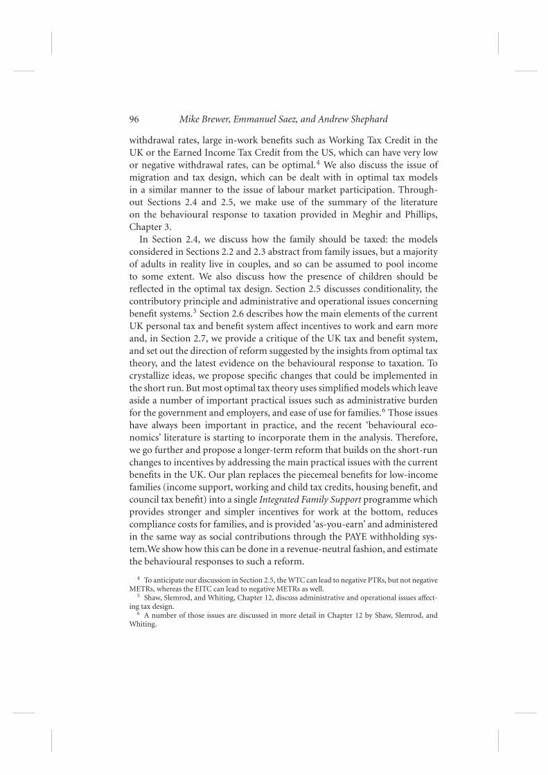
Table 2.2. Optimal tax rates and lump-sum grants
Redistribution strength Elasticity Average MTR Lump-sum grant (per year)
„ = 1 0.25 45% £5,580Rawlsian 0.25 73% £8,150„ = 1 0.50 31% £4,270Rawlsian 0.50 58% £6,760
Note: Authors’ calculation using formulae in text and FRS 2003–04 and SPI 2003–04.
variations in annual hours worked are a combination of participationresponses (whether a woman works at all in a given week), and intensiveresponses (changes in the hours worked per week).
But hours worked are not the only way in which taxable income canrespond to tax changes. For many individuals, the idea that the hourly wagecannot be affected by the amount of effort expended by the individual (asassumed in the theoretical models in Section 2.3) is too simplistic; earningscould respond to tax changes through changes in the hourly wage (whetherthrough bonuses, tips, job changes, or even by workers on piece rates work-ing faster) as well as hours worked. Taxable income reported to the rev-enue authorities, though, is not the same as gross earnings, and can varyin response to tax changes through changes in the form of compensation,the response of non-labour income, and changes in the amount of incomereported to the tax authorities, whether through avoidance or evasion. Saez(2002) argues that ‘elasticities of earnings with respect to the tax rate [at thebottom end] are . . . perhaps around 0.25’, and that: ‘there is little consensusabout the magnitude of intensive elasticities of earnings for middle incomeearners, although this elasticity is likely to be of modest size for middleincome earners and higher for high income earners. Gruber and Saez (2002)summarize this literature and display empirical estimates between 0.25 and0.5 for middle and high income earners’ (Saez (2002), p. 1057), althoughmost of this is focused on the US.
Figure 2.4A also displays an optimal schedule in the case where individuallabour supply is more responsive to changes in income (an elasticity of 0.5).The figure demonstrates that this would produce lower METRs across theearnings distribution, falling as low as 20%, with a top rate of 45% (slightlybelow the existing rate). The intuition for the difference here is simple: whenindividuals are more responsive to tax changes, they will react more to a givenMETR (reducing their labour supply by more), and this places a limit on howhigh METRs can go. Correspondingly, and as shown in Table 2.2, the benefitprogramme is less generous when the elasticity is higher.

Means-testing and Tax Rates on Earnings 115
0%
10%
20%
30%
40%
50%
60%
70%
80%
90%
100%
0
50,0
00
100,
000
150,
000
200,
000
250,
000
300,
000
350,
000
400,
000
450,
000
500,
000
Annual gross earnings, £
Mar
gin
al t
ax r
ate
Rawlsian
γ=1
Note: Authors’ calculation using formulae in text and FRS 2003–04 and SPI 2003–04.
Figure 2.4B. Optimal tax sensitivity, redistribution preference
Finally, we consider how the government’s preferences for redistributionaffect the optimal schedule (see Box 2.6 and the online appendix (see footnote14) for more detail). An interesting case to consider is known as the Rawlsiancase, which seeks to maximize the welfare of the least well-off member of soci-ety.25 As Figure 2.4B and Table 2.2 show, under this criterion, we would havea higher lump-sum grant and higher METRs across the entire distributionof earnings. Hence, rates are higher at the bottom, and are the same as theutilitarian case at the top. Therefore, with a Rawlsian criterion, the optimalshape becomes closer to an L- than U-shape.
Box 2.6. Expressing the preference for redistribution
In calculating social welfare, we first transform (money metric) utilities so thatwe allow for the possibility that the government attaches more weight to thewelfare gains of individuals whose level of utility is initially low. A convenientand simple way of capturing this concern for inequality is to transform original
(cont.)
25 The Rawlsian criterion can therefore be seen as a bound on the maximum level of redistri-bution that the government wishes to do; note that in the optimal tax model, even the Rawlsiangovernment has to raise revenue for some reason, and this places a limit on the size of the transferto the poorest in society.

116 Mike Brewer, Emmanuel Saez, and Andrew Shephard
Box 2.6. (cont.)
utilities u as follows:
u1−„
1 − „if „ =/ 1
log(u) if „ = 1
Social welfare is then obtained by summing these transformed utilities acrossindividuals. Whenever „ is positive, any increase in utility translates into a lessthan proportional increase in social welfare. When „ = 1, which is the case thatwe consider here, the government is placing twice as much weight on the utilitygains of an individual relative to another individual whose utility is twice ashigh. If concerns for inequality were even stronger, represented by say „ = 2,then they would be placing four times as much weight on the utility gains of theless well-off individual. When „ = 0, there is no concern for inequality; when „
gets very large, only the worst-off individual in society determines social welfare(the Rawlsian case discussed further below).
The form of individuals’ utility function is given in the online appendix (seefootnote 14), but note that it is quasi-linear in income, and so it does not displaydiminishing marginal utility of income, which can by itself provide a motivefor redistribution even if a government has a strictly utilitarian social welfarefunction.
2.3. OPTIMAL TAXES AND TRANSFERS WHEN THEREARE PARTICIPATION EFFECTS
The model described in the previous section assumes that individualsrespond to the tax and benefit system only by varying their earnings asa function of the net-of-tax rate they face (known as the intensive mar-gin/response). However, changes in whether people participate in the labourmarket at all (known as participation or extensive responses) are poorlycaptured within such a framework (see Blundell and MaCurdy (1999)).Indeed, following a small increase in the net gain of work, people tend toenter employment at, say, twenty or forty hours a week, rather than one ortwo hours. Such extensive labour supply responses are particularly impor-tant at the bottom of the income distribution, and can be incorporatedinto a model of labour supply using fixed costs of work (Heim and Meyer(2004)).

Means-testing and Tax Rates on Earnings 117
Participation effects are important: accounting for them radically mod-ifies the structure of optimal taxes for low income families from the oneobtained above (Diamond (1980), Saez (2002)). In this section, we out-line the key theoretical results, and then discuss recent applications usingUK data.
2.3.1. Theory
We continue to work with a simple labour supply model, but this timeindividuals only choose whether or not to work, and this decision dependson the relative rewards to working and not working (including the costs ofwork). The responsiveness of this decision to the financial rewards can besummarized in the elasticity of participation with respect to the net return towork, similar to the elasticity defined in Box 2.1. If individuals do work, theirearnings are fixed.
If the government implements a tax and benefit schedule that determinesthe disposable income of individuals both in and out of work, then anindividual chooses to work if the net return to work exceeds her cost ofworking.26 Consider the impact of a small rise in the PTR at a given levelof earnings. This reform affects only individuals with this earnings potential,because there are no intensive responses. As in Section 2.2.1, this reform hasthree effects on government tax receipts and welfare:
1. The reform increases the taxes paid by every taxpayer at the given levelof earnings who works, increasing government revenues.
2. Those extra taxes reduce the welfare of the workers who pay this extratax, with the value that the government places upon this dependentupon its redistributive preferences.
3. The tax rise induces some of the workers at this earnings level to dropout of work, and this has a cost.
At the optimal, these effects must balance. In the Appendix, we derive for-mally what this means for the optimal tax schedule, with the result presentedin Box 2.7.
26 Since individuals of a given ability level may differ in their costs of working, for any given taxsystem some of these individuals may choose to work and others not.

118 Mike Brewer, Emmanuel Saez, and Andrew Shephard
Box 2.7. Optimal tax rates with participation responses
Let g (z) denote the value the government places on increasing income of indi-viduals with income z. If the government values redistribution, then g (z) willfall as z rises.
Defining the participation tax rate as t(z) = (T(z) − T(0))/z, we can derivethe optimal tax rate as:
t(z)
1 − t(z)=
1
Á· (1 − g (z))
This formula is a simple inverse elasticity tax rule for the participation tax rateon work. The PTR decreases with the elasticity Á and with g (z), the social valueof marginal consumption for individuals earning z.
As Box 2.7 shows, the optimal average tax rate at any given earnings level willbe lower:
1. The more highly the government values income at that earnings level.
2. The higher is the participation elasticity (since it is not desirable to taxindividuals who adversely respond to reductions in their incomes).
A striking implication is that, if the government values redistribution—so that 1 − g (z) is negative—then the participation tax rate should be nega-tive for low earnings—in other words, low income workers should receivean earnings subsidy. Hence, in sharp contrast to the intensive model, theextensive model implies that earnings subsidies or work-contingent credits(such as the earned income tax credit or the working tax credit) should bepart of an optimal tax system.27
The intuition for this result can be understood as follows. Starting froma tax and benefit system with a positive participation tax rate for low-skilled workers, and suppose the government contemplates strengtheningwork incentives for low-skilled individuals by reducing the taxes that theywould pay when working. This has the following effects:
� The cut in taxes means that tax revenues fall, and this is a cost.� But the associated increase in income of low-skilled workers is viewed
positively by a government that values redistribution, because it wouldprefer these individuals to have income more than the average individual.By our assumption that we are considering low income individuals (forwhom g (z) exceeds 1), this benefit effect has to outweigh the costs ofreduced revenue.
27 This result is robust to introducing income effects, as formula (3) remains valid with incomeeffects: see Saez (2002a).

Means-testing and Tax Rates on Earnings 119
� The behavioural response from cutting the PTR is to induce somelow-skilled individuals to start working, and this increases governmentrevenue (because the individuals who move into work pay positivenet taxes).
Hence, this reform is unambiguously desirable, and the implication is thatpositive PTRs for low-income workers cannot be optimal.
These arguments were true for a model where the only response is along theextensive margin. A more realistic model which allows for both intensive andextensive effects is presented in Saez (2002a). To summarize the implicationsof such a model, consider the situation outlined above, where the governmentlowers taxes (which are currently greater than zero) for low-skilled workers. Ifthere are both intensive responses and extensive responses, then cutting taxeshere would induce some higher skilled workers to reduce their labour supply,as well as inducing some non-workers to work. Although the latter responseis a benefit to society, the former is a cost, and so cutting taxes has ambiguouseffects on labour supply and therefore overall social welfare. A governmentcontemplating strengthening incentives by cutting taxes facing low-incomeworkers must therefore weigh precisely the positive participation effect andthe negative intensive labour supply effect, and the model in Saez (2002) givesa precise formula for that trade-off.
Interpreting the participation response
The extension of the optimal tax model to allow for non-participation hasother applications. Two of those are tax evasion and migration.
To apply the model to tax evasion, our earlier concept of ‘earnings’ couldbe interpreted as ‘earnings reported to the government agency administeringtaxes and transfers’. Suppose that low-income earners can decide to workeither in the formal sector, where we assume full compliance with the tax andbenefit rules, or in the informal sector, where we assume full non-compliance.In that case, the decision to work or not work can be replaced by the decisionto work and report earnings, or to work informally and not report earnings.In that case, for a given level of tax enforcement efforts, our earlier analysis(and the formula presented in Box 2.7) remains valid. However, in such amodel, the government might recognize that some of all individuals report-ing no earnings are in reality working informally, and so might actually bebetter off than low-income workers in the formal sector. This may lead thegovernment to place a lower value on the consumption of individuals withno reported earnings than they do on workers with low reported earnings

120 Mike Brewer, Emmanuel Saez, and Andrew Shephard
(i.e., g (0) < g (z) for some z), and this would make subsidies for work evenmore likely to be optimal.28
Second, taxes and transfers might affect migration in or out of the coun-try. For example, high tax rates on skilled workers in continental Europemight induce some of them to move to the UK or the US where the bur-den of tax on high-income individuals may be lower, and generous ben-efits for lower-income individuals in certain countries might encouragemigration of low-skilled workers toward those countries.29 In the onlineappendix (see footnote 14), we discuss how the migration decision can beincorporated into optimal taxation models.
2.3.2. Evidence on extensive elasticities and empirical applications
Meghir and Phillips (Chapter 3) show that there is a wide range of participa-tion elasticities for women in the literature: ‘Aaberge et al. (1999), Arrufat andZabalza (1986) and Pencavel (1986) find results of 0.65, 1.41 and 0.77–0.89respectively using cross-sectional data-sets from Italy, the UK and the US, andusing significantly different modelling and estimation strategies. . . . Devereux(2004), however, finds a lower degree of responsiveness with the elasticity atthe median family income equal to 0.17.’ There is consensus, though, thatparticipation is more elastic amongst women from poorer families so that‘participation is likely to be the key margin of adjustment for poorer women’.
For men, the two studies of static labour supply cited by Meghir andPhillips (Chapter 3) suggest an elasticity close to zero, but they highlight thata separate literature on the effect of unemployment benefits on the durationof unemployment has consistently found that higher benefits lead to a longerperiod out of work. Even including these effects, though, they suggest theoverall participation elasticity for men is very close to zero, at 0.04. A dynamicmodel for young men in Germany (Adda et al. (2006)) gives a similarly lowparticipation elasticity (0.06). But Meghir and Phillips also provide theirown, new empirical evidence. This very clearly shows the heterogeneity ofresponses: for highly educated men, it is hard to reject the idea that the
28 However, subsidies for low-income individuals might induce individuals to over-report self-employment income. In the US, Saez (2002b) shows that the self-employed are much more likelythan wage earners to report income which makes them entitled to the maximum EITC payments,strongly suggesting that self-employed individuals manipulate their reported earnings to take advan-tage of the EITC, making use of a flexibility not available to wage earners.
29 Clearly, governments can use other tools to affect immigration, and such policies are takenhere as given. In the EU, emigration and immigration across EU countries is almost completelyderegulated, and so our analysis is particularly relevant in this context.

Means-testing and Tax Rates on Earnings 121
participation elasticity is zero, but the estimate for men with low educationalqualifications is 0.23 for single men, and 0.43 for men in couples.
There are very few empirical studies of optimal tax systems that incorpo-rate intensive and extensive responses: Saez (2002) is an example for the US.Of course, one approach to the second goal of this chapter—where we seek toapply the lessons from optimal tax theory to make recommendations for theUK tax and benefit system—would have been to use an optimal tax modelthat allowed for intensive and extensive responses to solve for the optimalschedule. We have not taken this approach, though, primarily because weneeded to reflect that the current tax system in the UK has different tax sched-ules for single people and couples, and schedules that vary by the number ofchildren, but also because we also consider the impact of the tax and benefitsystem on family formation and fertility, and administrative issues, and it isto these we turn in the next section.
2.4. HOW SHOULD TAXES AND BENEFITS TREAT‘THE FAMILY’?
The models we have considered thus far were based on individuals and soabstracted from family issues. In reality, a majority of adults live in couples,and can be assumed to share income to some extent. In this section, wediscuss how the family should be taxed, and how the presence of childrenshould affect taxes and benefits. See Boxes 2.8 and 2.9 for a discussion of howthese issues are currently treated in the UK.
Under a pure individual-based taxation, tax liability is assessed separatelyfor each family member and is therefore independent of the presence orincome of other individuals living in the family or household. At the otherextreme, in a system of fully joint taxation of couples, tax liability is assessed atthe family level, and depends on total family income (this is how income taxworks in the US, for example). Over the past three decades, there has been aninternational trend from joint to individual taxation of husbands and wives,and today the majority of OECD countries use the individual as the basicunit of taxation (income tax in the UK moved from being family-based toindividual-based in April 1990). But tax credits and transfers for low-incomefamilies in the UK are based on total family income, as are the equivalentwelfare benefits in most other OECD countries, and there has been muchless impetus to move to an individual-based system for assessing transfers. Ofcourse, there are many other ways of designing a tax and benefits schedule

122 Mike Brewer, Emmanuel Saez, and Andrew Shephard
for individuals that varies with the presence of a partner than a fully joint taxand benefit system, and many EU countries with individual tax systems havesome form of recognition of marriage or the presence of a partner (see DiTommaso et al. (1999)).
In general, there are several important points to be considered whendesigning taxes and benefits for individuals who can live either alone or ina couple:
1. If there is any sharing of resources within a family, a person with alow income living with a high-income spouse is better off than anotherwise-equivalent person living with a low-income spouse. There-fore, if the government values redistribution, two adults earning thesame ought not to be taxed the same if their partners’ incomes are verydifferent. This redistributive principle is achieved to a limited extent byhaving a progressive income tax system based on family income, sinceit imposes higher average tax rates on adults with high-income spousesthan on otherwise-identical people with low-income spouses. By con-trast, an individual-based income tax does not meet this redistributivecriterion: it imposes the same tax burden on individuals irrespective oftheir partner’s earnings.
2. If there are economies of scale in households, so that two adults livingapart could achieve the same standard of living with less income if theylived together, then this arguably provides a reason for the tax system totake account of whether individuals are in a couple or not, presumablyby taxing individuals more when they are living as a couple than whenthey are living alone.
3. Family-based income tax and benefit systems are highly likely to cre-ate a marriage (or cohabitiation) subsidy or penalty, as the net taxliability of the two adults might change if they decide to cohabit ormarry. This is well-documented in the US, where the income tax sys-tem is family-based for married couples, but not for cohabiting cou-ples. Because the US tax system is progressive—in other words, thetax burden rises as income rises—couples with very unequal incomes(such as single-earner couples) benefit from a marriage subsidy, whilecouples with similar incomes (such as two-earner couples) face a mar-riage penalty. Although the marriage penalty/subsidy attracts substan-tial public attention, it becomes relevant for optimal taxation only if thedecision to marry is sensitive to those fiscal incentives. Hoynes (com-mentary on this chapter) concludes that ‘overall, the research [mostly

Means-testing and Tax Rates on Earnings 123
using US data] finds tax effects on marriage that are consistent withthe theoretical predictions but are small in size’ (these studies are citedin Eissa and Hoynes (2004)); a related literature finds that marriageis also sensitive to the financial incentives inherent in welfare systems(almost always anti-marriage incentives), but that the elasticities aresmall (see Hoynes (1997)). Overall, then, Hoynes concludes that ‘theestimated elasticities with respect to the tax-induced financial incen-tives to marry (and divorce) are small’. However, even if marriage orpartnership decisions are relatively insensitive to fiscal consequences,we might expect that how individuals report their family circumstancesto the government authorities would be affected by sufficiently largecohabitation penalties or subsidies.30
4. The empirical literature has shown that the labour supply of secondaryearners is more responsive to taxes than that of primary earners (seeMeghir and Phillips, Chapter 3, or Blundell and MaCurdy (1999)).Therefore, the earnings of secondary earners should be taxed at alower rate than the earnings of primary earners for efficiency reasons.31
This goal is achieved to some extent by a progressive individual-basedincome tax, since primary earners have higher incomes and hence tendto face higher METRs than secondary earners. By contrast, a family-based tax and benefit system generates identical METRs across mem-bers of the same family, and thus does not meet this efficiency principle.
5. Any tax and benefit system other than a fully joint system will giveindividuals in a couple a tax incentive to equalize their asset holdingsor income streams. While this might be a deliberate policy intention, aconsequence is that it gives couples an opportunity to reduce their taxburden by transferring assets from an adult with the higher METR tothe lower METR.
Deriving general optimal tax results for couples is, in general, extremelycomplicated. Kleven et al. (2006) consider a simple optimal tax model for
30 In the UK, Her Majesty’s Revenue and Customs and the Department for Work and Pensionsboth estimate the extent of money lost to such fraud or error relating to the presence of a partner:these estimate that £67 million was overpaid in income support, jobseekers allowance and thepension credit, £30 million in housing benefit (both in 2005–06) and £320 million overpaid in taxcredits (in 2004–05) (DWP (2007a) and HMRC (2007b)). Powerful circumstantial evidence thatsuch fraud exists comes from the fact that the UK government is paying child-contingent supportto between 5 and 10% more lone parent families than are thought to live in the UK (Brewer et al.(2008b); Brewer and Shaw (2006)).
31 This is in line with the traditional Ramsey principle of optimal taxation that commodities withrelatively more elastic demands should have relatively lower tax rates. See also Boskin and Sheshinski(1983) and Alesina and Ichino (2007).

124 Mike Brewer, Emmanuel Saez, and Andrew Shephard
couples where the primary earner chooses only how much to work (as inthe models outlined in Section 2.2) and the secondary earner chooses onlywhether or not to work (as in the models outlined in Section 2.3). In contrastto the separable and linear tax system in Boskin and Sheshinski (1983), theyconsider a fully general joint taxation system. Naive intuition suggests that,for redistributive reasons, the participation tax rate on the secondary earnershould be higher when the earnings of the primary earner are larger, as thecontribution of the secondary earner’s income to the family’s well-being isminimal. However, the authors show that the reverse is true: the participationtax rate on the secondary earner should be decreasing with the earnings of theprimary earner and, symmetrically, the primary earner should face a lowerMETR if his or her spouse works.
The correct intuition is the following: conditional on the earnings of theprimary earner, two-earner couples are always better off than one-earnercouples. Hence, the government would like to redistribute from two-earnercouples to one-earner couples. The value of such redistribution is largerfor couples with low primary earnings because the contribution of the sec-ondary earner to household utility is then more important. Therefore, theredistributive virtue of taxing secondary earnings is actually higher at thebottom of the primary earnings distribution, explaining why the tax rateon a secondary earner is decreasing with the primary earner income. If thetax schedule for two-earner couples is seen as the base schedule, the optimalschedule for one-earner couples is obtained from that base schedule by intro-ducing a tax allowance for non-working spouses that is larger for coupleswith low primary earnings than for couples with high primary earnings. Thisshrinking tax allowance generates an implicit tax on secondary earners whichdecreases with primary earnings.
This result suggests that a progressive joint income tax system goes inthe wrong direction, and that neutral individual taxation is closer to theoptimum. However, it is important to note that, in practice, benefits for low-income families are almost always based on joint family income, and thephasing-out of those programmes creates implicit taxes on secondary earnerswhich are decreasing with primary earnings. For example, a secondary earnerin the UK with modest earnings would face a relatively high (average andmarginal) tax rate when his or her partner’s earnings are low, because thesecond adult’s earnings reduce the family’s tax credit entitlement as well asbeing subject to income tax and National Insurance contributions, and wouldface a relatively low (average and marginal) tax if their partner’s earningsare high, because the secondary earnings are subject only to the individualincome tax and NICs. Hence, the results in Kleven et al. (2006) suggest that

Means-testing and Tax Rates on Earnings 125
the broad way in which tax and benefit systems of many OECD countriestreat the incomes of a couple, including that of the UK, are consistent withoptimal tax results.
Box 2.8. Marriage and cohabitation penalties in the UK tax andtransfer system.
As we discuss in Section 2.6, the UK has individual assessment for incometax, but welfare programmes and the child and working tax credit are assessedagainst the joint income of co-resident couples, where legally married or not.There are currently very few tax-induced marriage penalties or subsidies in theUK.a However, there are substantial so-called cohabitation or couple penaltiesor subsidies in the UK: these arise because welfare benefits and tax credits areassessed against the joint income of cohabiting couples, whether legally marriedor not.b The same structural features that lead to such cohabitation penaltiesalso give differences between the incentives to work facing the first and secondearner in a couple. Typically, the PTR of the second earner will be considerablylower than that of the first earner (see also Figure 2.6A), but the direction ofrecent reforms has tended to increase PTRs of second earners as entitlement totax credits has risen in real terms (see Brewer (2007)).
a See Bowler (2007); some groups have argued that there should be more subsidies: see Social JusticePolicy Group (2007).
b Such couple penalties or subsidies are usually shown either by calculating the change in nettransfers from the state that two adults would experience if they were to cohabit—a complicatedcalculation that requires assumptions on how housing costs and labour supply would change uponcohabitation—or by calculating the change in net transfers that a cohabiting couple would experienceif they (fraudently) claimed to be living apart. See Anderberg et al. (2008); see also Kirby (2005) andDraper (2007).
2.4.1. Collective labour supply model
How disposable income is allocated among family members raises interest-ing issues. Empirical findings by Lundberg et al. (1997) show that givingan allowance for children directly to the mother instead of giving it to themain earner through a reduction in taxes increased spending on childrensignificantly. This shows that families do not fit what is called the ‘uni-tary model’, whereby a family acts as if all the adults in it care about thesame things. Many other models of behaviour of couples are possible, andChiappori (1988, 1992) developed a model where consumption is allocatedwithin family members in an efficient way (so that it is not possible to makeone member in the family better off without making another worse off),but that the power each family member has in the decision-making process

126 Mike Brewer, Emmanuel Saez, and Andrew Shephard
depends on their relative incomes or on who is entitled to the governmenttransfers (this is known as a collective labour supply model).
How does this affect our analysis? Suppose, for example, that husbandshave too much power within a couple, and get too much control over howincome is used relative to their spouses, and suppose that the governmentwould like to achieve a fairer distribution of consumption within families.If the government wants to increase parents’ spending on children, Blundell,Chiappori, and Meghir (2005) show that what matters is how the marginalwillingness to spend on children differs across parents. If mothers have ahigher marginal willingness to spend, then it is valuable to transfer resourcesfrom husband to wife. The empirical analysis of Lundberg et al. (1997) sug-gests that this can be done at no fiscal cost simply by switching who is thenominal recipient of the benefit in the family (and without altering the totaldisposable income of the family). Therefore, in sharp contrast to the previousmodels we have considered so far, this within-family redistribution does notcreate any efficiency costs (as long as the within-family bargaining is efficient,as assumed in Chiappori (1988, 1992).
These results suggest that within-family distributional issues could beaddressed by transfers from wallet to purse, but leaving unchanged the totallevel of transfers going to low-income families. The issue of transferringbetween high- and low-income families is not fundamentally affected bybargaining issues within the family.
2.4.2. The treatment of children
In Box 2.9 we briefly discuss actual child-contingent transfers in the UK.There are various arguments why the optimal tax schedule should dependupon the presence of children:32
1. The presence of children could be used as a tag (Akerlof (1978)), if thepresence of children in a family is correlated with the parents’ abilityto pay taxes, or because it is correlated with the labour supply elasticity(we cited evidence in support of the latter in Section 2.2).33
2. To the extent that children represent a cost to their families, so that afamily with children needs more disposable income than one without
32 Similar arguments can be made for matters such as old age, or long-term sickness or disabili-ties, but we do not explore these here.
33 Note that this argument does not say whether, for a given level of income, a family withchildren should face a lower average tax burden or METR than a family without in an optimaltax system, merely that they could be different.

Means-testing and Tax Rates on Earnings 127
to reach a given standard of well-being, then there is an argumentthat this should be reflected in the optimal tax schedule, so that fora given family income level, the presence of children should reducethe family’s tax liability or increase the transfers received. But this isnot a universally held viewpoint: certainly children do cost money, butgiven that there is a degree of choice in having children, there must besome benefits to families too, it can be questioned why society shouldcompensate families for a particular lifestyle choice;34 given the benefitsthat arise from having children, compensating families for the extracost of having children cannot be justified as easily as compensatingfamilies for the extra costs imposed by long-term sickness or disability,for example.
3. A society may feel a responsibility for children’s well-being directlybecause they are unable to affect their parents’ income, and there istherefore an argument for an optimal tax system to provide a meansof insuring children against growing up in a household with a lowincome (this argument is strengthened if there are costs to societyas a whole from having children grow up in a household with lowincome).
However, it is also possible that decisions on whether to have children (andif so, how many) are affected by the generosity of child-contingent transfers. Ifso, this introduces another aspect of behaviour which can be distorted by thedesign of the tax system, potentially leading to efficiency costs.35 Surveyingrecent evidence, Brewer et al. (2007b) conclude that fertility can be responsiveto financial considerations, but the implied elasticity is low.36 If fertility doesrespond to financial incentives, then this introduces another dimension to theoptimal tax problem.
34 This argument was made forcibly by Dilnot et al. (1984).35 Clearly if there are benefits (or costs) to society as a whole from the presence of children which
parents do not take account of when making fertility decisions, and if fertility decisions are affectedby the generosity of the tax and transfer system, then this may provide a rationale for using the taxsystem to subsidize (or tax) children (this is a standard argument for using the tax system to correctfor externalities: see Fullerton, Leicester, and Smith, Chapter 5).
36 In the US, there is little conclusive evidence that welfare benefits or the EITC have anyeffect on fertility (see Hoynes (1997) and Baughman and Dickert-Conlin (2007)) but studies ofspecific programmes in other countries have shown there to be small responses of fertility to child-contingent transfers (see Laroque and Salanié (2005) and Milligan (2005)).

128 Mike Brewer, Emmanuel Saez, and Andrew Shephard
Box 2.9. Child-contingent transfers in the UK
The UK tax and benefit system varies markedly with the presence of and numberof children. At the time of the Meade Report (Meade, 1978), the UK govern-ment was replacing child tax allowances and a programme known as familyallowances with child benefit: a non-means-tested cash payment for all childrenalmost always paid direct to the child’s mother. But child benefit is no longerthe most expensive programme for supporting children thanks to the growth,since 1997, of means-tested tax credits conditional on the presence of children.a
Overall, then, child-contingent transfers in the UK are now more means-testedthan universal, and are higher for the first child than subsequent children (boththese features have been accentuated since 1997).
Because there have been large increases in entitlements to welfare benefits andtax credits for families with dependent children but none for those without, thesize of net transfers that is conditional on having children has risen substan-tially since 1997: the real value of child-contingent transfers per child grew byaround 50% between 1997 and 2003, more than it had risen by in the previoustwenty-two years, and Brewer, Ratcliffe, and Smith (2007) provide new evidencesuggesting this increase has led to a rise in fertility amongst couples likely to beeligible for such programmes.
a See Adam and Brewer (2004) and Adam et al. (2007). These changes have come about becausethe current UK government is particularly concerned about the high (by international and historical)levels of relative child poverty, and this concern—and the tough quantified targets that accompaniedit—has led to very large real increases in entitlements to welfare benefits and tax credits for familieswith dependent children since 1998 (see Brewer et al. (2008b)).
2.5. ADMINISTRATIVE AND OPERATIONAL CONCERNSIN OPTIMAL TAX DESIGN
In this section, we discuss whether and how a benefit system for low-incomeindividuals should be complemented by requirements (backed up with sanc-tions) for failing to accept suitable jobs and/or work a sufficient number ofhours, and other administrative and operational issues concerning benefitsor in-work credits.
2.5.1. The role of conditionality and active labour market policies
A general trend throughout many OECD countries in the 1990s was theadoption of active labour market policies in order to encourage work amongwelfare recipients and the unemployed. Such policies range from training

Means-testing and Tax Rates on Earnings 129
programmes, assistance in finding jobs, or requirements, backed up withsanctions, for welfare recipients to look for work and to accept reasonablejob offers.37
If participation tax rates for low-skilled workers are high, then the taxand benefit system discourages low-skilled work. In that context, it wouldbe socially desirable to induce those who are just indifferent between work-ing and not working to start working, since doing so would raise revenue(a gain to society), and the cost to the individuals of having to work isnegligible. Obviously, strengthening financial incentives is one way to achievethis goal, as we discussed in Section 2.3. However, conditionality or activelabour market policies can provide alternative tools that the governmentcan use to induce work. If the direct cost of providing ALMPs or enforcingjob-search requirements plus the welfare cost of forcing individuals to dothings they would not have chosen otherwise is smaller than the fiscal savingsobtained from having more people work, then such policies are sociallydesirable.38 The general principle follows the theory of quotas and rationingdeveloped by Guesnerie and Roberts (1984): goods that are subsidized by theoptimal tax system should be rationed. In a system where participation taxrates for low-skilled workers are high, then being out of work is effectivelysubsidized, and should be rationed.
Two points should be noted. First, in reality, the welfare costs of forcingsome individuals to work is higher than it is for others, and it might bedifficult for the government to target precisely the individuals who do facelow costs of working (and therefore for whom requirements to seek andaccept job offers are most likely to be welfare-improving for society), andthose active labour market policies might generate substantial welfare costsif, for example, they require beneficiaries with very high costs of working tostart working. A crude but common way to achieve such targeting is to usefamily and disability status.39
Second, if the optimal tax system is such that the participation tax rateamong low-skilled individuals is low (and even more so if it is negative as our
37 A very large empirical literature analyses such programmes, and Kluve et al. (2007) provides acomprehensive survey of this literature and meta-analysis for policies in European countries.
38 HC 32 (2007–08) compares the direct cost of providing different New Deal programmes in theUK in 2005–06 with the net tax savings from getting participants into work, and finds that most ofthe UK’s active labour market programmes are not worthwhile (the calculation takes only a short-run view of the fiscal savings, but on the other hand, it does value the costs of making individualswork when they would have preferred not to).
39 For example, after the 1996 welfare reform in the US, welfare recipients were required to enrolin training programmes or work part-time unless they had very young children. In the UK, the con-ditions that apply to claimants of out-of-work benefits are different for lone parents, those who havea long-term sickness or a disability, and other individuals (although the current government has pro-posed changes to reduce these differences). See Cm 7290 (2006–07) for the UK government’s currentstrategy.

130 Mike Brewer, Emmanuel Saez, and Andrew Shephard
previous analysis suggested), then the desirability of using such active labourmarket policies is weakened as the tax savings from inducing people to workare small (or even negative, if the PTR is negative). In the optimal tax modeldeveloped in Section 2.2.2, it is desirable to induce out-of-work high-skilledindividuals to start working, but in reality, active labour market policies rarelytarget high-skilled individuals.
This discussion (like previous sections) assumes the government maxi-mizes a social welfare function that depends only on individual utilities; theapproach to optimal taxation pioneered by Mirrlees is considered ‘welfarist’in the sense that it disregards any information not related to individuals’well-being or welfare. In such a model, if individuals make a well-informeddecision not to work given the tax schedule facing them, then that decisionshould be respected by the government. In contrast, a non-welfarist approachto optimal taxation allows for the government to use a criterion for evaluatingsocial welfare that is different from the preferences of the individuals. Clearly,departures from the welfarist approach to optimal non-linear income taxa-tion may lead to very different implications for taxation design. For example,Kanbur, Keen, and Tuomala (1994) consider an optimal tax problem wherethe objective of the government is to reduce poverty defined using a stan-dard income-based poverty index.40 Moffitt (2006) argues that the historyof redistributional policy in the US suggests that the government valueswork per se and given this, considers an optimal taxation problem where thegovernment has a direct objective to maximize the number of individuals inwork (the same conclusion would almost certainly be drawn about recent UKgovernments). In this setting, earnings subsidies are often optimal, and workrequirements emerge as an instrument for improving the government’s viewof social welfare (see the commentary by Robert Moffitt).
Box 2.10 discusses the extent to which transfers in the UK can be viewed asconditional, rather than unconditional, transfers.
Box 2.10. Conditionality in the main transfer programmes
The shape of the budget constraint for those with no or very low earnings (andhence PTRs for all workers) in practice depends on whether the benefits areconditional or unconditional.
Of the benefits mentioned above, HB/CTB and CTC are paid to all who areincome-eligible, and the WTC is paid to all who are income-eligible and where
40 By contrast, a welfarist government might be deeply concerned about, for example, povertymeasured by a standard income-based poverty index, but only as an intermediate objective.

Means-testing and Tax Rates on Earnings 131
one person in the family works some minimum number of hours a week: forthese programmes, claimants are not required to do any other activities as acondition of receiving benefit. However, conditions do apply to those claimingIS or JSA (which are two identically structured programmes for people whoare out of work and on a low income). Claimants of JSA have to be availablefor work, actively seeking work, and have agreed a jobseeker’s agreement withJobcentre Plus; furthermore, people may be unable to claim JSA if they left theirprevious job voluntarily, or were sacked for misconduct. In principle, this meansthat people who do not make sufficient effort to look for work, or who turndown reasonable offers of work, can lose their entitlement to benefit for between1 and 26 weeks (with exceptions made for vulnerable groups). Claimants of ISmay have to attend periodic meetings at a Jobcentre Plus office, but do not haveto look for work as a condition of receiving benefit; however, only some groupsare allowed to claim IS, the main ones being people who are sick or disabled,people who are caring for a sick or disabled individual, and lone parents whosechildren are all aged under 7.a
Adults who are incapable of work through sickness or disability may receiveincapacity benefits (incapacity benefit and income support on the grounds ofdisability), continued receipt of which is conditional only on attending periodicmeetings at a Jobcentre Plus office. New claimants from April 2008 must insteadclaim the Employment and Support Allowance, which has requirements onclaimants, backed up with sanctions for non-compliance.
a At the time of writing in 2008, lone parents could claim IS until their youngest child reached 16,but this will fall to age 7 by October 2010. See Cm 7290 (2006–07).
2.5.2. The assessment period and timing of taxes and transfers
In most countries, individual income taxes are assessed on annual income,and transfers often assessed on a monthly basis (in the UK, weekly). Standardeconomic models predict that families should budget over long time peri-ods, by borrowing (or using credit) and saving. If families have fluctuatingincomes but are able to smooth consumption over time by borrowing andsaving, then income assessed over a longer period of time is a better measureof economic welfare or well-being than income assessed over a short periodof time.
In reality, costs of using financial services and other credit market failures,low levels of literacy, numeracy and financial education, and self-controlproblems with savings all create significant departures from the standardmodel. These departures are likely to be more prevalent amongst low-income

132 Mike Brewer, Emmanuel Saez, and Andrew Shephard
families, and tend to lead to such families budgeting consumption overshort periods of time, such as a month or a fortnight. It therefore seemsdesirable to operate transfers for low-income families on a high-frequencybasis, and operate taxes on higher incomes on a lower frequency, such asannual.
Another important aspect is the timing of tax payment or benefit receiptrelative to the period of earnings assessment. Because of imperfect credit mar-kets and some families’ imperfect ability to budget (as described above), manyfamilies would be unable to pay a significant level of tax if it is not withheldat the time they receive the earnings: this is why setting up tax withholdingsystems operated by employers is key to implementing broad-based taxes (orsocial insurance contributions) on earnings.41 In this way, income tax canbe withheld throughout the year at levels which are approximately correct,and a small adjustment made once a year if the amount withheld does notcorrespond to the actual tax liability. A similar argument applies to the designof benefits: the closer is the timing of payment to the period of assessment, thebetter targeted is the benefit; paying credits through a single annual payment(as almost always happens with the EITC) can be very inefficient if familiesare credit constrained.42
One way of aligning the timing of payment to the timing of assessmentis to administer benefits for workers through the income tax system; sucha scheme can also have lower administrative and compliance costs relativeto traditional welfare programmes and relative to the child and workingtax credits in the UK, discussed further below. For example, a (refundable)tax credit could be administered through a system of ‘negative withholding’,where the revenue authorities fund employers to top up earnings instead ofwithholding taxes. Having an automatic system of benefit payments may alsoreduce stigma costs for recipients.43
However, the experience of the first two years of the working and childtax credits in the UK (see Box 2.11), the Advance EITC in the US, or Prime àl’Emploi in France, all show that such a system will cause difficulties if there is
41 We use ‘withholding’ in the same sense as Shaw, Slemrod, and Whiting, Chapter 12.42 It is possible that the prospect of a large annual lumpsum tax refund induces families to
borrow against the forthcoming tax refund with high interest costs. Indeed, surveys show that US taxrefunds received by low- and moderate-income families are used primarily for paying down debts.Alternatively, one-off tax refunds can be seen as forced savings devices which allow low-incomefamilies with self-control problems to save for purchasing consumer durables or investing in humancapital. Empirical work has not yet been able to distinguish those two scenarios. It is striking tonote, however, that there is little demand for such forced savings devices in the UK where transfersare paid monthly or fortnightly.
43 Exactly as taxpayers disliked interactions with the tax collector in past centuries, welfarerecipients today dislike the close scrutiny required to qualify for such transfers.

Means-testing and Tax Rates on Earnings 133
a significant risk that families incur an overpayment which they have to repayto the government. This fear leads the vast majority of EITC recipients in theUS to opt to receive it annually in arrears, and the UK government changedthe way tax credits depend on income in 2005 so that they are predominantlybased on the previous tax year’s income (except where income falls), meaningthat most rises in income should not lead to over-payments (although thischange was predicted to reduce the number of over-payments by just a third).But such a design makes tax credits rather like a retrospective benefit schemebased on annual income, and this means the credits are then not as welltargeted as they could be.44
Box 2.11. The administration and operation of tax credits in the UK
In-work programmes increased in importance during the early to mid-1990s,partly as a response to the growing prevalence of lone parent families. But theirimportance changed beyond recognition between 1999 and 2003. The workingtax credit now supports working families with or without children with a lowincome, and the child tax credit is now received by around 90% of all familieswith children. These tax credits are administered by Her Majesty’s Revenue andCustoms (HMRC), but they have many elements which feel much more liketraditional welfare programmes: they are jointly assessed, paid regularly anddirectly to recipients’ bank accounts, and do not reduce income tax liabilities.
The administration of tax credits has been extensively criticized, with a cross-party group of Members of Parliament concluding in early 2008 that ‘there islittle evidence that [HMRC] has the scheme under control. Many claimantscontinue to struggle to understand tax credits and why they are overpaid.There have been many complaints about the process of recovering overpay-ments and the Ombudsman continues to receive and uphold a large numberof complaints.’a
These administrative problems mostly derive from policy choices, so it isworth discussing these briefly. One of the predecessors of the child and workingtax credit was Working Families’ Tax Credit (WFTC). WFTC awards wereretrospective, so entitlement to WFTC, having been determined, was paid for6 months regardless of any changes in the family’s circumstances; any changesin circumstances were reflected in the next award if the family re-applied after6 months. Because awards were based on verified information, there was noneed to re-assess awards.
(cont.)
44 Many of these issues were discussed in detail when the UK government proposed mergingworking families’ tax credit (a 6-monthly retrospective transfer programme) and the children’s taxcredit (an annual transfer implemented through PAYE) to form the child and working tax credit: seeBrewer et al. (2001) and Whiteford et al. (2003) for more discussion. See also Brewer (2006).
134 Mike Brewer, Emmanuel Saez, and Andrew Shephard
Box 2.11. (cont.)
But the retrospective nature, combined with the 6-month gap between assess-ments, meant that payments need not have reflected current circumstances,and these, plus the perceived compliance costs to families of providing verifiedearnings details twice a year, were the main motivations behind the introductionof the child and working tax credits. Their design reflects an attempt to reconcilethese tensions. The principle of the child and working tax credits is that theyshould depend on current family circumstances, and income in the current year.But the tax authorities do not know the details on which tax credit entitlementsdepend (the earnings of all adults in the family, the number of children, whetherany adult is working for 16 or 30 or more hours a week, and how much is beingspent on childcare) so tax credits rely on two things: first, there is a responsibilityon claimants to tell HMRC when there is a change in their circumstances—suchas whether they are living with a partner, how many children they have, and alsowhat they are spending on childcare—within a month of its happening. Second,tax credits are likely to be based on the claimant’s previous year’s annual income:claimants whose income is lower than last year’s can have tax credits assessedon their best estimate of their current income, but claimants whose income ishigher than the previous year can have tax credits assessed on the previous year’sincome, provided that is within £25,000 of their current annual income.
a HC 300 2006–07. See also Brewer (2006) and references therein.
2.6. THE CURRENT HOUSEHOLD TAX AND BENEFIT SYSTEMIN THE UK
This section describes the inherent work incentives for working-age adultsin the UK tax and benefit system that arise from income tax, employer andemployee National Insurance contributions (the payroll tax), the workingand child tax credits, and other benefits.45 Box 2.12 summarizes the keychanges since Meade (see also Adam, Browne, and Heady, Chapter 1, andreferences therein).46
45 There is more detail on individual taxes in Adam, Browne, and Heady (Chapter 1) and onindividual transfer programmes in O’Dea et al. (2007). We do not show the schedule affectingthose over the state pension age, nor do we discuss health- or disability-related transfers: the maindifferences for those above state pension age are: there is no payroll tax on earned income, thereare higher personal allowances for income tax, welfare programmes are more generous, and health-related transfers are more important.
46 Adam et al. (2006) shows the distribution of key work incentive measures has changed overtime; their measures of work incentives exclude employer NI, however. Adam, Browne, and Heady,Chapter 1, show how tax and transfer changes have affected key work incentive measures.

Means-testing and Tax Rates on Earnings 135
Box 2.12. The main changes to the UK tax and transfer system sincethe Meade Report
Much has changed in the personal tax and benefit system in the UK since theMeade Report in 1978, but we would highlight three particularly importantdevelopments:
First, statutory rates of tax have fallen at the top, but marginal effectivetax rates (METRs) have not necessarily fallen. In 1978, the highest marginalincome tax rate on earned income was 83%; a decade later, it had fallen to40% (with extensions of National Insurance contributions over this period,the overall marginal tax rate on top earnings, before considering the impactof consumption taxes, is now 47.6%). But this tells us only about the changein the marginal tax rate facing the very richest in the UK: between 1974 and1978, the mean income of the richest 1% of adults in the UK was not highenough for the highest marginal rate to be applicable, but the mean incomein the top 0.1% was. In fact, across the whole population, statutory incometax rates are generally lower than in 1978, but METRs across the whole dis-tribution are not necessarily lower now than in 1978, partly because of theexpansion of income-related in-work programmes, and partly because taxallowances have not kept pace with growth in earnings (a phenomenon knownas fiscal drag) (see Adam, Browne, and Heady, Chapter 1, and Adam et al.(2006)).
Second, income tax is assessed at the individual level, rather than jointly, butmany married or cohabiting couples in the UK still face some form of jointassessment of their incomes, thanks to the expansion of income-related in-work programmes, and of means-tested benefits for those aged 60 or more.Income tax became individualized in 1990, and there have been few politicalpressures to reverse this reform. Instead, there has been a trend of increasinguse of means-tested benefits that depend upon the joint income of a co-residentcouple, whether legally married or not (see the commentary by Hoynes forfurther discussion).
There has been an expansion of in-work programmes or refundable taxcredits conditional on work. In fact, the UK has had a programme to supportlow-income working families since 1972, but the importance of benefits tofamilies who are working is much greater now than at the time of the MeadeReport.
Figure 2.5A-1 shows how the annual net income of a lone parent withtwo children varies with the annual employer cost (ie, annual earnings plusemployer NICs).47 While this is not intended to be a typical family, it does
47 Throughout this section we assume that there are no childcare costs. Owing to the hours rulesin the tax system, the actual budget constraint will depend upon the wage received. We assume

136 Mike Brewer, Emmanuel Saez, and Andrew Shephard
0
10,000
20,000
30,000
40,000
50,000
60,000
Cost to employer, £/year
0 10,000 20,000 30,000 40,000 50,000 60,000 70,000
Net
inco
me,
£/y
ear
budget constraint
budget constraint (inc. housing benefit)
Notes: Assumes a lone parent with two children, paying £80 per week in rent, no childcare costs, averageBand C council tax, and with a wage of £5.52 per hour. Incomes are calculated under the April 2008 taxand benefit system with announced changes to the higher-rate threshold and UEL, but without the £600rise in the income tax personal allowance.
Figure 2.5A-1. Budget constraint, lone parent
illustrate some of the key features of the UK tax and benefit system (Box 2.13discusses how the tax and benefit system varies across different familytypes).
Figures 2.5B-1 and 2.5C-1 show how the associated participation tax rate(PTR) and METR vary with earnings for the same specimen family type.They also show the empirical relationship between PTRs and METRs and theemployer cost for all working lone parents, given the underlying demographicstructure, employment patterns, and distribution of earnings in the UK (themain reason why the empirical distribution differs from the hypotheticalrelationship is that, on average, lone parent families have fewer than twochildren, and children serve to raise PTRs and extend the range of incomeover which a high METR applies).
that the wage rate is equal to the minimum wage (as of October 2007) of £5.52 per hour. Thebenefits system works on a weekly basis, and the tax system on an annual basis, but the figureshave assumed both work on an annual basis. The figures show the 2008–09 tax system beforethe £600 rise in the income tax personal allowance, and with the small changes to the UpperEarnings Limit for employee NICs and the income tax higher-rate threshold scheduled for April2009.

Means-testing and Tax Rates on Earnings 137
0%
20%
40%
60%
80%
100%
120%
Cost to employer, £/year
Par
tici
pat
ion
tax
rat
e
PTRPTR (inc. housing benefit)empirical PTR
10,0000 20,000 30,000 40,000 50,000 60,000 70,000
Notes: Example PTRs as for Figure 2.1A. Empirical PTRs based on all workers in families where no adultis aged 60 or over in FRS 2004–05 with net incomes calculated using TAXBEN.
Figure 2.5B-1. Participation tax rate, lone parent
0%
0 10,000 20,000 30,000 40,000 50,000 60,000 70,000
20%
40%
60%
80%
100%
120%
Cost to employer, £/year
Mar
gin
al t
ax r
ates
MTRMTR (inc.housing benefit)empirical MTR
Notes: Example PTRs as for Figure 2.1A. Empirical PTRs based on all workers in families where no adultis aged 60 or over in FRS 2004–05 with net incomes calculated using TAXBEN.
Figure 2.5C-1. Marginal tax rates, lone parent

138 Mike Brewer, Emmanuel Saez, and Andrew Shephard
0
10,000
20,000
30,000
40,000
50,000
60,000
Cost to employer, £/year
0 10,000 20,000 30,000 40,000 50,000 60,000 70,000
Net
inco
me,
£/y
ear
budget constraint
budget constraint (inc. housing benefit)
Notes: Assumes paying £80 per week in rent, average Band C council tax, and with a wage of £5.52 perhour. Incomes are calculated under the April 2008 tax and benefit system with announced changes to thehigher-rate threshold and UEL, but without the £600 rise in the income tax personal allowance.
Figure 2.5A-2. Budget constraint, single no children
0%
0 10,000 20,000 30,000 40,000 50,000 60,000 70,000
20%
40%
60%
80%
100%
120%
Cost to employer, £/year
Par
tici
pat
ion
tax
rat
e
PTR
PTR (inc. housing benefit)
empirical PTR
Notes: Example PTRs as for Figure 2.1A. Empirical PTRs based on all workers in families where no adultis aged 60 or over in FRS 2004–05 with net incomes calculated using TAXBEN.
Figure 2.5B-2. Participation tax rate, single no children

Means-testing and Tax Rates on Earnings 139
0%0 10,000 20,000 30,000 40,000 50,000 60,000 70,000
20%
40%
60%
80%
100%
120%
Cost to employer, £/year
Mar
gin
al t
ax r
ates
MTRMTR (inc.housing benefit)Empirical MTR
Note: Example PTRs as for Figure 2.1A. Empirical PTRs based on all workers in families where no adult isaged 60 or over in FRS 2004–05 with net incomes calculated using TAXBEN.
Figure 2.5C-2. Marginal tax rates, single no children
0%10,000 20,000 30,000 40,000 50,000 60,000 70,000
10%
–10%
20%
30%
40%
50%
60%
70%
80%
90%
100%
Cost to employer, £/year
Par
tici
pat
ion
tax
rat
e
without children: partner doesn't work
without children: partner works
with children: partner doesn't work
with children: partner works
Note: Empirical PTRs based on all workers in families where no adult is aged 60 or over in FRS 2004–05with net incomes calculated using TAXBEN. Assumes tax system as described in notes to Figure 2.1A.
Figure 2.6A. Empirical Participation tax rates, couples with and without children

140 Mike Brewer, Emmanuel Saez, and Andrew Shephard
10,0000 20,000 30,000 40,000 50,000 60,000 70,000
Cost to employer, £/year
Par
tici
pat
ion
tax
rat
e
without children: partner doesn't work
without children: partner works
with children: partner doesn't work
with children: partner works
0%
10%
20%
30%
40%
50%
60%
70%
80%
90%
100%
Note: Empirical PTRs based on all workers in families where no adult is aged 60 or over in FRS 2004–05with net incomes calculated using TAXBEN. Assumes tax system as described in notes to Figure 2.1A.
Figure 2.6B. Empirical Marginal tax rates, couples with and without children
Box 2.13. Generalizing to other family types
Descriptions of the marginal rate schedule can be heavily dependent on thechoice of family circumstances, but we can make some general comments aboutvariations across family types (see also Figures 2.5A-2, 2.5B-2, 2.5C-2 and 2.6Aand 2.6B):
The schedule of METRs would be identical to that shown for a primary earnerin a couple with children, but PTRs would be higher, because such families areentitled to more JSA/IS than lone parents when they do not work but no moreWTC when they do work.
The presence and number of children has a large impact on the METR sched-ule (and a smaller impact on PTRs) for low to middle earners: each additional(fewer) child would increase (decrease) the point at which the METR falls from73.4% to 38.8% by £5,346 a year (personal earnings in 2008–09).
Families without dependent children are not entitled to tax credits until theywork 30 hours a week, and so METRs would be lower (and PTRs a lot higher)than those for otherwise-equivalent families with children working between 16and 29 hours a week.
Because of the various hours rules in the UK tax and benefit system, assuminghigher hourly wages given a value of employer cost measured weekly would

Means-testing and Tax Rates on Earnings 141
change the pattern of METRs and PTRs at the bottom of the earnings distri-bution, but not at the top, where income tax, National Insurance contributions,and tax credits depend only on weekly or annual earnings.
Generalizing across other forms of income is harder: unearned income istreated differently from earned income in IS/JSA, and by National Insurancecontributions, but treated similarly to earned income by income tax and taxcredits; self-employment profits are treated differently from earnings fromemployment by National Insurance contributions, but not by income tax orbenefits.
They illustrate the following features of the UK tax and benefit system:
1. The PTR is 0% for very low earnings and then increases rapidly. Thisreflects the structure of the main means-tested benefits for familieswith no earnings and who work no more than 15 hours a week (Job-seekers’ Allowance (JSA) and/or Income Support (IS)48). For familieson JSA/IS, a 100% METR applies after a small earnings disregard (£5a week for single adults, £10 a week for couples, £20 a week for loneparents): families therefore face no direct financial incentive to increasetheir earnings above the very low disregard unless they earn enoughto exhaust fully entitlement to IS/JSA, or they work a sufficiently highnumber of hours to qualify for the working tax credit. In April 2008, asingle adult aged 25 or over would receive £60.50 a week in JSA. Receiptof these benefits also confers entitlement to various benefit-in-kindprogrammes, the most important of which is entitlement to free schoolmeals.49
2. Hours rules are an extremely important part of the benefit system inthe UK:50 the most important ones are that individuals working 16or more hours may not claim JSA/IS, and individuals with (without)children working 16 (30) or more hours may instead claim working taxcredit.51 Figures 2.5B-1 and 2.5B-2 show that these hours rules lead to
48 There is also a short-term non-means-tested jobseekers’ allowance for those who have paidsufficient National Insurance contributions, but a minority of JSA recipients qualify for this.
49 The loss of these benefits-in-kind can substantially increase PTRs; the difficulty is modellingtheir value to individual families. For a qualitative study, see Community Links et al. (2007).
50 In principle, making the working tax credit means-tested against weekly earnings and condi-tional on working 16 or more hours a week means it is more closely focused on low-wage workersthan would be the case if it were conditional solely on having positive earnings. In practice, theremay be very few high wage workers who would wish to work small numbers of hours if there werean earnings-based in-work credit, and so there may be little efficiency gain from having an hoursrule. Furthermore, under the current rules for the WTC, hours of work are self-reported (althoughpotentially verifiable if HMRC consults with employers).
51 The take-up rate for the WTC for those without children is extremely low, at 20% (25% byvalue; see HMRC (2007a)).

142 Mike Brewer, Emmanuel Saez, and Andrew Shephard
a striking discontinuity in the PTR schedule: after reaching a maximumat the point just before entitlement to JSA/IS is exhausted, the PTR fallssubstantially at 16 hours work a week (there is a further discontinuityat 30 hours a week—annual earnings of £8,611 for a minimum wageworker—when an additional credit in the WTC is payable).
3. Families with dependent children receive child-contingent supportthrough a non-means-tested child benefit, and most receive morethrough a means-tested fully refundable child tax credit.52 In 2008–09, a lone parent and two children with no private income wouldreceive £183 a week from income support, child benefit, and childtax credit combined, three times as much as the single adult with nochildren.
4. The shape of the budget constraint for low to middle earners variesconsiderably by whether a family is entitled to the means-testedbenefits known as housing benefit and council tax benefit (together,HB/CTB) (Box 2.14). Families who are receiving JSA/IS are automat-ically entitled to the full amount of HB/CTB, but once JSA/IS hasbeen exhausted, HB/CTB are withdrawn at a rapid rate. This can dra-matically reduce the gain to work: in Figure 2.5A-1, for example, netincome increases by over £2,626/year when the earner works 16 hoursa week, but with housing costs of £4,160 / year, this is reduced to£312/year.53
5. For most people, METRs are determined by the rates of income taxand National Insurance contributions. Income tax (20%) and employeeNICs (11%) are both liable when annual earnings reach £5,435 a year(£104.52 a week) to give a METR of 31% (plus 12.8% on the employer,or 38.3% overall).54 This increases to 47.7% (41% plus 12.8% onthe employer) when earnings are sufficiently high for the higher rateof income tax to be liable (from April 2008, this will be £41,435 ayear, but the government has already announced a real rise in this
52 In the rest of this section, we use children to mean dependent children, which is currentlydefined as children under 16, or aged 19 or under in full-time education or approved trainingschemes.
53 The 2008 Budget—which took place as this chapter was being finalized—announced that earn-ings disregards in housing benefit and council tax benefit would effectively be increased substantiallyfor families with children from October 2009. This is not reflected in Figures 2.5–2.6.
54 If an employer pays £1 in notional gross earnings, then the employer actually pays out 112.8p,and the individual actually receives 69p, with the government receiving 43.8p. The overall METR istherefore 43.8/112.8 or 38.3%.

Means-testing and Tax Rates on Earnings 143
threshold from April 2009 which we allow for in our reform proposalsin Section 2.7).55
6. But METRs are considerably higher for families entitled to tax creditsor HB/CTB. Once annual earnings have reached £6,420, entitlement totax credits begins to fall, and this increases the METR by 39 percentagepoints (ppts) to 70% (with the 12.8% on the employer, this reaches73.4% overall). For a family with two children and a full-time earner,the 70% (or 73.4%) METR falls back to 31% (or 38.3%) once grossannual earnings reached £28,150. But what complicates—and raises—METRs even further is the way this combined income tax–NI–tax creditMETR interacts with HB/CTB: to give an example, someone facinga combined income tax–NI–tax credit METR of 70% and entitled toHB/CTB would face an METR of 95.5% (plus 12.8% on the employerside, or 96% overall): see Box 2.14.
Box 2.14. Housing benefit and council tax benefit
Housing benefit is a rental subsidy programme which can potentially cover thefull cost of renting (subject to locally determined rent ceilings), but where actualentitlement depends upon family income and household composition.a Coun-cil tax benefit is a very similarly structured programme that provides a(potentially 100%) rebate on council tax payments. Hereafter we refer to theseprogrammes together as HB/CTB.
The withdrawal rate in HB is 65%, and in CTB, 20%; these are cumulative,but they apply to net income, not gross income, and so the 20%/65%/85%withdrawal rate of CTB/HB/both combined is not added to the combinedincome tax–NI–tax credit METR, but instead applied to whatever earnings areleft. For example, someone facing a combined income tax–employee NICs–taxcredit METR of 70% and on the taper of both HB and CTB would lose 85% ofthe remaining 30%, giving a total MTR of 95.5% (plus 12.8% on the employerside, or 96% overall). Someone with a combined income tax–employee NICsMETR of 31% and on the taper of CTB would lose 20% of the remaining 69%,giving a total MTR of 44.8% (51% with employer NI).
a In the private rental sector, the rules for HB changed in April 2008 so that the maximum entitle-ment depends on household size and composition (and locality), and not on the actual rent paid.
55 When joint family earnings are between £50,000 and £57,783, the family element of the childtax credit is withdrawn at a rate of 6.7%, giving a slightly higher METR of 47.7% plus 12.8% onemployer, or 53.6% over this range.

144 Mike Brewer, Emmanuel Saez, and Andrew Shephard
Table 2.3. Distribution of participation tax rates amongst workers, 2008–09 tax andbenefit system
Centile of distribution of PTRs
10th 25th 50th 75th 90th Mean
Single, no children 0.31 0.40 0.42 0.47 0.63 0.44Couple, no children
Partner not working 0.28 0.35 0.45 0.55 0.67 0.45Partner working 0.18 0.25 0.30 0.35 0.41 0.29
Lone Parent 0.01 0.25 0.44 0.55 0.66 0.36Couple with children
Partner not working 0.40 0.48 0.56 0.64 0.78 0.55Partner working 0.15 0.29 0.39 0.50 0.57 0.37
Notes and sources: Authors’ calculations based on FRS 2004–05 with net incomes calculated usingTAXBEN. Sample is all workers. Adults in families with anyone aged 60+ are excluded. Assumes tax systemas described in notes to Figure 2.1A.
Table 2.3 shows the distribution of work incentives measures for variousfamily types (and see also Figures 2.5B-1, 2.5B-2, 2.5C-1, 2.5C-2 and 2.6Aand 2.6B). It shows that:
� METRs and PTRs are generally higher for families with children thanthose without with identical incomes.56
� PTRs are generally lower for adults whose partner is in work than for thesole earner in a couple.
2.7. A PLAN FOR REFORMING TAXES AND TRANSFERSIN THE UK
In this final section, we first suggest a set of changes to the existing tax andbenefit structure that could be made immediately and that address problemswe identify with the work incentives inherent in the current system. We thenset out a more radical and comprehensive set of structural changes to thetax and benefit system that attempt to deal not only with the work incen-tive issues, but also with the administrative failings that we identify. None of
56 One slight exception is that low-earning lone parents can face lower PTRs than low-earningsingle adults without children: this is because WTC requires fewer hours of work for lone parentsthan low-earning single adults without children, and because the interaction of child maintenancepayments with IS/JSA and WTC means that lone parents receiving child maintenance payments canface very low or negative PTRs if they do not receive HB/CTB.

Means-testing and Tax Rates on Earnings 145
the reforms described below would apply to those aged 60 or over, nor do wepropose specific changes for those with long-term sickness or disabilities, nordo we address how conditionality should be applied to out-of-work benefitsnor how welfare to work policies should be designed.
As we discussed earlier, one direct way to arrive at an optimal tax andbenefit schedule for the UK would be to use an optimal tax model for the UKthat reflected extensive and intensive responses. But such a model would mostlikely miss out on some of the considerable heterogeneity between differentsorts of families in the tax and benefit schedules (as the schedule differs bythe number of adults and the number of children), and it would be even morecomplicated to allow for responses other than to taxable income (for example,to reflect that household formation may be sensitive to tax incentives) and toallow for concerns over administrative and compliance costs. Instead, we havesought in this section to apply the lessons from optimal tax theory combinedwith the best available evidence on the scale of behavioural responses, andour knowledge of the incentives inherent in the existing UK tax and benefitsystem.
In formulating these suggested reforms, we have been guided by the fol-lowing points or principles, discussed earlier in this chapter:
� For certain groups, such as second earners and individuals with low levelsof education, extensive responses are likely to be more important thanintensive responses (see Section 2.3.2).
� The responsiveness of hours worked to the tax system is very low formost groups, and perhaps zero. The responsiveness of taxable earningsis greater, with an elasticity of perhaps 0.25 for low- and middle-incomeearners, rising for high-income earners (see Section 2.2.3).
� There may be little or no scope for raising METRs applying to top earnersin the UK. The current tax system in the UK has METRs from incomeand NICs that rise modestly: the combined tax rate on earned incomerises from 31% to 41% (from 40.6% to 47.7% including employer NI)when earnings reach £41,435 (April 2008). Section 2.2.3 showed that,with reasonable preferences for redistribution, METRs should rise in theupper part of the earnings distribution if the elasticity of taxable incomewith respect to tax rates is constant across income groups. Our numer-ical simulations (Figures 2.4A and 2.4B) showed that, if elasticities wereconstant and modest in size—our numerical example used an elasticityof 0.25—then increasing tax progressivity of the current UK tax systemby adding yet an additional higher tax rate for the richest 1% would bedesirable. However, our empirical analysis reported in Table 2.1 suggests

146 Mike Brewer, Emmanuel Saez, and Andrew Shephard
that the relevant elasticity of the richest 1% might exceed 0.25, in whichcase it is undesirable to increase top METRs because doing so wouldreduce government revenues. We therefore do not propose changes tothe METR affecting top incomes.
� We take it for granted that the income tax system will remain individual,reflecting the extremely strong current political consensus in supportof individualized income tax, and we conclude that the redistributivebenefit of jointly assessed transfers for lower-income families outweighsany efficiency losses (see Section 2.4).
The present UK tax and benefit system described in Section 2.5 suffers fromfour important defects:
� Participation tax rates for low levels of earnings are high: for mostgroups, they are close to 100% before individuals are entitled to theworking tax credit, and they remain high even with the working taxcredit. These PTRs appear much too high in a context where opti-mal tax theory suggests that the participation tax rate should be low,possibly even negative, at low levels of earnings, so as to encouragepeople to move into work. And PTRs for families potentially entitled toHB/CTB remain extremely high (over 70%) even at medium and highincomes.
� The phasing-out of the working and child tax credit, which operateson top of income tax and NICs, generates METRs of 73.4% includingemployer NICs (higher if also entitled to HB/CTB) for a large number oflow to moderate earners; such a high METR is highly likely to be abovethe optimal rate even with modest behavioural responses.
� The main means-tested programme to help with housing (housingbenefit) has an extremely high withdrawal rate, administrative diffi-culties, and problems of misperception which deter low-income workingfamilies from claiming it (Turley and Thomas (2006)), and, by its design,predominately affects a minority group in society—tenants of socialhousing—who we might expect to have low earnings capabilities anda weak labour market attachment, and therefore relatively high laboursupply elasticities.
� While the system for administering income tax and NICs in the UK issimple and efficient, the systems for administering child and workingtax credits, and those for housing benefit and council tax benefit, areadministratively burdensome for claimants, relatively expensive for thegovernment, and prone to large amounts of fraud and error: all mean

Means-testing and Tax Rates on Earnings 147
that neither is as well-targeted on the economic situation of beneficiariesas it could be.57
We set out reforms that could address these shortcomings in the followingtwo sections.
2.7.1. Immediate changes to household taxes and transfers
There are a number of straightforward steps that could be taken within thecurrent system in order to address the key work disincentives.58
� Increase the level of earnings disregards (the amount of earnings a personis allowed to earn before benefits are withdrawn) in all of the means-tested benefits (in order of priority, HB/CTB then JSA/IS) to reducePTRs on earnings of less than £90 a week for all, and on higher earn-ings for individuals receiving HB/CTB: these groups currently face veryweak incentives to work at all.59 An increase of HB/CTB disregards to£50/week would cost £1.7 billion a year, to the value of 16 times theminimum wage would cost £4.3 billion. Duplicating this in JSA/IS wouldcost an extra £0.3 billion or £0.6 billion respectively. This policy shouldlead to an increase in employment, but it would also extend eligibility toHB/CTB to many more working families, and so this measure should beconsidered only alongside measures dramatically to speed up processingtimes for HB/CTB claims, or a move to fixed or retrospective HB/CTBawards (to eliminate the problem of overpayments). Hopefully suchmeasures, plus the clear signal sent by a large disregard, would themselvesdo much to increase the take-up rate of HB/CTB amongst eligible work-ing families. Higher disregards in IS/JSA would also increase the numberof people eligible for such benefits both through its immediate effects
57 Tax credits are expensive to administer (HMRC spent £587 million in 2006–07 to administernet spending of £18.7 billion, a ratio of 3.13%, compared to a ratio of 2.12% to administer WFTC, itsmuch smaller predecessor (see Cm 6983 2006–07 and HC 626 2006–07) tax credits have the highestrates of fraud and error in central government (£1 billion to £1.3 billion in 2004–05 out of totalspending of around £16 billion; HMRC, (2007b)), they can often serve to increase (rather than cut)volatility of income (Hills et al. (2006)), and there remain concerns about their impact on recipients(see HC 1010 (2006–07)).
58 These are not all novel proposals: Bell et al. (2007) analyse large increases in the earningsdisregards in transfer programmes affecting lone parents, and HC 42-I (2007–08) recommends themfor all family types; Adam et al. (2007) analyse increases in the working tax credit; Brewer (2007)analyses an extra credit for second earners in the working tax credit, as proposed by CM 6951 (2006–07) and Cooke and Lawton (2008).
59 As this chapter was being finalized, Budget 2008 announced an effective rise in the earningsdisregard for families with children of £20 a week for those with one child, and more for largerfamilies. This clearly reduces the cost (and impact) of our proposal.

148 Mike Brewer, Emmanuel Saez, and Andrew Shephard
(because it extends eligibility up the income distribution), and after con-sidering the behavioural response (because it makes working fewer than16 hours and claiming IS/JSA relatively more appealing than working16 or more hours and not claiming IS/JSA). Higher disregards in IS/JSAmight be less appealing, then, if a government had a direct objective toget people off IS/JSA, which it might do if it had a non-welfarist objectivefunction (see earlier section), or if the cost of administering IS/JSA weremuch higher than the cost of administering transfers for low-incomefamilies in work.
� Introduce an additional earnings disregard in tax credits for secondearners (or an additional credit in the working tax credit for fami-lies with two earners). This would reduce PTRs for secondary earners,particularly those with children. Giving each individual their own earn-ings disregard of £6,200 in tax credits would cost £1.3 billion beforeany behavioural change. The downside of this policy would be that itmerely shifts upwards the range of income over which second earnerscan expect to face a very high METR through the withdrawal of taxcredits alongside payment of income tax and National Insurance. How-ever, this seems justifiable given the strong evidence that participationelasticities are relatively high for second earners in couples with children,and that the extensive response is more important than the intensiveresponse.
� Reduce the withdrawal rate in child and working tax credits. This wouldreduce METRs and PTRs for individuals receiving the working or childtax credits, most of whom will be earning more than £90 a week. Acut from 39% to 34% would cost £1.4 billion before any behaviouralresponse. It would increase the number of individuals who face highMETRs through a withdrawal of tax credits on top of income tax andNICs, but our assessment is this is acceptable if it permits the combinedtax credit–income tax–NICs withdrawal rate to fall from its current highlevel of 73.4% (including employer NI), and it if acts to lower PTRs forlow-earning families.60
60 In the UK, most high METRs occur when income tax and NICs are liable at the same time astax credits are withdrawn. One way of solving this problem is to introduce large tax allowances,so that income tax is not deducted until tax credits are fully withdrawn; this change could beaccompanied by a rise in the tax credit withdrawal rate. This reform is appealing because it allowswell-off families to receive support through tax cuts administered automatically through PAYE,whilst focusing the part of the programme that pays out cash on the families with the lowest incomes.Compared to the current system, though, such a change is expensive, because it effectively grants taxallowances to families previously too rich to receive much or any tax credits, and it would only bepossible if the system of tax allowances were based on family, not individual, circumstances.

Means-testing and Tax Rates on Earnings 149
� Increase the working tax credit for groups other than lone parents (thelevel of the working tax credit for low-earning lone parents currentlyexceeds entitlement to IS/JSA if they did not work, leading to low ornegative PTRs at low earnings; no increase is needed here on efficiencygrounds). This would lower PTRs for low-earning individuals eligible forWTC. Equalizing WTC rates with JSA/IS rates would cost £3.2 billion;halving the gap would cost £1.6 billion. Two downsides of this policyare that it would increase the number of individuals who face a with-drawal of tax credits on top of income tax and NICs, and that it wouldreduce the gain to work for some second earners in couples (so directlyoffsetting the impact of the additional earnings disregard in tax creditsproposed above). However, the rationale for recommending this policyis that these downsides would be outweighed by the increase in thenumber of adults working, as participation tax rates are cut for eligiblefamilies.
Of course, all of these changes would mean the government paying outconsiderably more in transfers or tax credits.61 We do not at this stage proposeoffsetting changes to increase tax revenue or reduce spending on transferselsewhere. However, we have suggested these reforms on efficiency (ratherthan equity) grounds, and so it follows that any widespread tax rise (such as arise in VAT, income tax, or National Insurance) to fund these tax cuts shouldstill lead to a reform package that is desirable on efficiency grounds (in otherwords, it should be possible to find a revenue neutral set of tax and benefitchanges that leads to a overall increase in aggregate earnings).62
These reforms have suggested themselves on efficiency grounds, notbecause we are seeking to redistribute to particular groups. But whether theseproposals seem sensible to the government will obviously depend on theirown priorities for redistribution, so Tables 2.4A and 2.4B show the distribu-tional impact of these policies, and the average gain for different family types,assuming no change in behaviour, and ignoring the impact of any revenue-raising measures to pay for them (which could be chosen to have any desireddistributional effect).
61 Note that all the costs have been estimated assuming no behavioural change, and that onlyone reform at a time is implemented. However, the reforms, and therefore their costs, interact: a£50 disregard in all means-tested benefits plus the three tax credit changes would cost just over£8.8 billion).
62 Furthermore, it might be appropriate to reduce spending on child benefit (or the familyelement of the child tax credit) in order to pay for at least some of these reforms, given thatfamilies with children tend to benefit more than families without, and given that these reformssuggested themselves on efficiency grounds, and not from a desire to redistribute more to particulargroups.

150 Mike Brewer, Emmanuel Saez, and Andrew Shephard
Table 2.4A. Distributional impact of reforms (% gain in net income)
Income Reform
DecileGroup
Increaseearningsdisregards
Raise WTCentitlements
Cut taxcredits taper
2nd adultdisregard in taxcredits
All reforms
Poorest 2.88 0.26 0.00 0.00 3.132 2.90 1.69 0.24 0.10 4.553 2.08 3.41 1.27 1.05 7.014 0.85 3.39 1.61 1.65 7.845 0.36 1.13 0.58 0.69 4.466 0.15 0.19 0.19 0.09 1.707 0.10 0.07 0.06 0.01 0.368 0.06 0.03 0.02 0.00 0.129 0.02 0.01 0.01 0.00 0.04Richest 0.00 0.00 0.00 0.00 0.00
Notes: Authors’ calculations based on FRS 2004–05 data and the TAXBEN micro-simulation model.Pre-reform tax system as described in notes to Figure 2.1A.
Table 2.4B. Distributional impact of reforms by family type (% gain in net income)
Reform
Family Type Increaseearningsdisregards
Raise WTCentitlements
Cut taxcredits taper
2nd adultdisregard intax credits
All reforms
Singles, no children 0.45 0.66 0.08 0.00 1.32Couples, no children 0.17 0.20 0.05 0.00 0.45Couples, with children 0.51 1.06 0.52 0.67 3.21Singles, with children 0.58 0.00 0.69 0.00 1.26
Notes: Authors’ calculations based on FRS 2004–05 data and the TAXBEN micro-simulation model.Pre-reform tax system as described in notes to Figure 2.1A.
2.7.2. Radical reform: the Integrated Family Support
The radical reform plan we propose goes one step further. It is designednot only to be targeting net tax cuts where incentives to work are cur-rently at their weakest but also to simplify administration and enforcementfor the government, and to reduce the compliance costs of employers andclaimants.
The centrepiece of our new tax and benefit system is a new programme,called the Integrated Family Support (IFS), which acts as a replacement for

Means-testing and Tax Rates on Earnings 151
child and working tax credit, income support/JSA, child benefit, housingbenefit, and council tax benefit.
The key features are as follows (there are more details on how it wouldwork in the online appendix (see footnote 14), but at this stage, we donot claim that we have identified or resolved all the operational andadministrative difficulties):
� Integrating most of the current benefits means that claimants can feelmore secure about continuing to receive transfers when their circum-stances change, and also removes the problems that can occur whenthe benefits interact (this particularly applies to the current interactionbetween tax credits and HB/CTB); these should reduce the compliancecosts of claimants. It should also mean fewer opportunities for fraud andsimplify administration and enforcement for the government.
� The maximum entitlement to the IFS would be family based, and wouldbe the sum of a family component (different for single adults andcouples), a child component (depending on the presence and number ofdependent children), and a housing component (depending on whetherthe family rents or owns, and on the local rental and council tax levels).This structure broadly reflects the current set of maximum entitlementsprovided through transfers and tax credits.
� The IFS allowance would be means-tested based on family income, butthere would be an individual earnings disregard of £90, or just over 16hours work at the current minimum wage.63 This disregard would applyto each adult in the family, so each of the two adults in a couple couldearn up to £90 and still keep the maximum IFS allowance. The aim ofthis, which echoes our suggested immediate reforms, is to lower PTRs—potentially to zero for low-earnings work—in order to encourage labourmarket participation amongst those currently not working.
� The IFS would be paid directly by the government to eligible low- andmoderate-income families, but the withdrawing of the IFS would beachieved, for the vast majority of families, through the existing (andaugmented) system of income tax and NI withholding.64 The IFS wouldnot be an annual system, but instead be operated on a non-cumulativebasis, with a weekly or monthly periodicity, so maximum entitlements
63 We describe the reform in 2008–09 prices (i.e., as if it were an alternative to the April 2008tax and transfer system), although we include in the base system for costing the reform the smallchange to the Upper Earnings Limit for employee NICs and the income tax higher-rate thresholddue in April 2009. However, this chapter was written before the £600 rise in the income tax personalallowance for 2008–09 was announced in May 2008.
64 We use the word ‘withholding’ in the same sense as in Shaw, Slemrod, and Whiting, Chapter 12.

152 Mike Brewer, Emmanuel Saez, and Andrew Shephard
would be determined weekly or monthly, and the withdrawal woulddepend on the earnings in each pay period. The aim is to ensure thatthe IFS is more transparent and provides more certainty than child andworking tax credits.65
� There will be two taper rates for the IFS: 30%, if the family is receivingonly the child and family elements, or 45% if the family is receivingthe housing element. These imply a lower overall METR than currentlyapplies to families entitled to tax credits and/or HB/CTB. This is in linewith our earlier conclusion that METRs for low to middle earners are fartoo high, even if behavioural responses are modest.
� This system does not do away with under- or over-payments, but theirincidence should be much reduced compared to the current systems.Similarly, end-of-year reconciliations will still be needed, although theseought to be combined with the self-assessment process for income tax(as they would only be needed for relatively well-off families receivingthe IFS). If, for various reasons, a family is under-withheld, the govern-ment would not ask for an immediate repayment, but could graduallyreduce the balance over time through reasonable reductions in futureIFS payments.
Financing the IFS, and its effect on household incomes
The substantial increase in the earnings disregard of the IFS relative to thecurrent system for IS/JSA, HB/CTB and in the working tax credit for secondearners, the effective cut in the withdrawal rates of HB/CTB and tax credits,and the extension of the IFS to groups currently eligible for neither IS/JSAnor tax credits all cost a significant amount.
For the reform to be revenue neutral before behavioural responses, thereneed to be net tax rises elsewhere. In this proposal, this has been achieved by:
1. Subsuming child benefit and the family element of the child tax creditwithin the IFS, and thereby removing both from better-off familiesthrough a means test.66
65 It would clearly be much simpler if the IFS was an annual, retrospective scheme, because thenit could be aligned fully with income tax. But doing this would mean that IFS payments could beweakly related to families’ circumstances, and this is significantly at odds with the principles oftransfer programmes in the UK.
66 There would then be no difference in the net taxes paid by well-off families with childrenand those without children, which makes sense if children are not seen as imposing extra costs: seethe discussion in Section 2.4. A version that retains child benefit would cost an extra £3.3 billion,and therefore it would be necessary to increase the basic rate of income tax by around 1 ppt to berevenue-neutral.

Means-testing and Tax Rates on Earnings 153
Table 2.5. Parameters of the IFS reforms
Single adult £50Couple £80Amount per child £50Supplement for first child
Lone parent family £30Couple family £20
Earnings disregard (for each adult) £90
Withdrawal rates†
IFS 30%HB/CTB 15%
Income tax and National Insurance thresholdsPersonal allowance/primary threshold £4,680/yr (£90/wk)
§ Weekly values unless stated otherwise.† Rates applied to gross income in excess of disregard.
2. Lowering the income tax personal allowance and the point at whichNICs start to be due to the IFS disregard of £90 a week.
3. Increasing the basic rate of income tax by 1 ppt.
4. Setting family and child entitlements to the IFS that are below thecurrent rates of JSA/IS and child tax credit, but higher than the currentrates of working tax credit.67
The key parameters are shown in Table 2.5.68
The effect of the IFS on household incomes
Figures 2.7A–2.7D show how the budget constraint for some specimen fam-ilies would change under the IFS. The main implication of the IFS is thatit starts withdrawing means-tested support at higher income levels than thepresent system, and then withdraws it more slowly. This strengthens the veryweak work incentives currently created by aggressive means-testing, but it
67 The last of these changes leads to losses for some low-income families with no private income.A version of the IFS where the family and child elements of the IFS are set at the existing ratesof IS/JSA and child tax credits (so as to produce no change in net transfers to families with noprivate income) would cost an extra £6 billion a year, and would imply considerable gains for low-earning adults without children, and all but the richest couples with children. To make this revenue-neutral would require increasing the basic rate of income tax by nearly 2 ppts (after considering thebehavioural responses).
68 Estimates of the cost of the IFS have been made assuming no behavioural change, and that allbenefits and tax credits are taken up. The second of these assumptions may understate the cost ofthe IFS; if the IFS succeeds in having a lower compliance burden for families, then some currentlynot claiming tax credits or HB/CTB when in work may be induced to do so.

154 Mike Brewer, Emmanuel Saez, and Andrew Shephard
0
0 10,000 20,000 30,000 40,000 50,000 60,000
10,000
20,000
30,000
40,000
50,000
60,000
Cost to employer, £/year
Net
inco
me,
£/y
ear
base budget constraint (inc. housing benefit)
IFS budget constraint (inc. housing benefit)
Notes: ‘Base budget constraint’ based on tax system as described in notes to Figure 2.1A. ‘IFS budgetconstraint’ based on tax system as described in text.
Figure 2.7A. IFS Reform, budget constraint, lone parents
0
0 10,000 20,000 30,000 40,000 50,000 60,000
10,000
20,000
30,000
40,000
50,000
60,000
Cost to employer, £/year
Net
inco
me,
£/y
ear
base budget constraint (no housing benefit)
IFS budget constraint (no housing benefit)
Notes: ‘Base budget constraint’ based on tax system as described in notes to Figure 2.1A. ‘IFS budgetconstraint’ based on tax system as described in text.
Figure 2.7B. IFS Reform, budget constraint, one earner couple with children

Means-testing and Tax Rates on Earnings 155
0
0 10,000 20,000 30,000 40,000 50,000 60,000
10,000
20,000
30,000
40,000
50,000
60,000
Cost to employer, £/year
Net
inco
me,
£/y
ear
base budget constraint (inc. housing benefit)
IFS budget constraint (inc. housing benefit)
Notes: ‘Base budget constraint’ based on tax system as described in notes to Figure 2.1A. ‘IFS budgetconstraint’ based on tax system as described in text.
Figure 2.7C. IFS Reform, budget constraint, single no children
00 10,000 20,000 30,000 40,000 50,000 60,000
10,000
20,000
30,000
40,000
50,000
60,000
Cost to employer, £/year
Net
inco
me,
£/y
ear
base budget constraint (no housing benefit)
IFS budget constraint (no housing benefit)
Notes: ‘Base budget constraint’ based on tax system as described in notes to Figure 2.1A. ‘IFS budgetconstraint’ based on tax system as described in text.
Figure 2.7D. IFS Reform, budget constraint, one earner couple without children

156 Mike Brewer, Emmanuel Saez, and Andrew Shephard
Table 2.6. Distributional impact of IFS (% gain in net income)
Decilegroup
Overallpopulation
Singles nochildren
Couples nochildren
Couples withchildren
Loneparents
Poorest 4.6 4.1 11.8 1.4 3.72 4.3 6.2 6.7 3.6 2.43 4.8 2.4 5.4 6.1 4.14 4.0 3.0 3.8 5.1 2.75 0.9 2.1 0.9 0.1 1.26 −1.7 1.3 −0.1 −4.6 0.37 −2.4 0.5 −0.4 −6.2 −0.28 −2.2 1.4 −1.2 −5.4 −2.59 −1.6 0.9 −1.2 −3.9 −3.2Richest −1.2 −0.4 −1.1 −2.1 −1.5
Note: Based on uprated data from the Family Resources Survey 2004–05 and the Institute for FiscalStudies’ tax and benefit micro-simulation model, TAXBEN. Tax systems described in notes to Figure 2.7A.
does bring many more people into the scope of means-testing on top ofincome tax and NICs.
Given the focus on strengthening the very weak work incentives for thoseon HB and CTB, there is a substantial shift in resources between those notentitled to HB and CTB to those who are (in practice, the vast majority ofhouseholds are liable to CT and therefore entitled to CTB, but only renters areeligible for HB). Whether the IFS reform implies an unacceptable distortionto the housing market—by increasing rent subsidies, and doing nothing forhome-owners—takes us outside the scope of optimal tax theory and intoissues related to housing policy in the UK, but addressing this (perceived oractual) distortion would require either reducing the generosity of housingbenefit, or extending it to home-owners so that it is tenure-neutral (withan accompanying general rise in tax to pay for this). Similarly, it is beyondthe scope of this chapter to consider whether council tax itself should bereformed; if it were made less regressive, then it might be possible to scrapcouncil tax benefit.
Table 2.6 shows the impact of the IFS on net incomes of working-ageadults, by family type, and by decile group of equivalized income of working-age adults before any consideration of behavioural effects. The main impactsof the IFS reform on net incomes are as follows.
� The maximum entitlements to the IFS are a little higher than currenttax credit entitlements but lower than current IS/JSA rates (except forlone parents), and this leads to losses for IS/JSA recipients with no othersources of income. However, the fact that the IFS is made available

Means-testing and Tax Rates on Earnings 157
without any hours rules means that some low-income individuals(particularly single adults aged 25 or over with no children and workingunder 30 hours a week) currently entitled to neither IS/JSA nor taxcredits gain substantially.
� Low-income families entitled to HB/CTB tend to gain because the equiv-alent support is withdrawn more slowly under the IFS.
� Better-off families with children tend to lose as support currently pro-vided through the non-means-tested child benefit is now tapered awayas part of the IFS.
� All taxpayers lose slightly as the income tax personal allowance and theNICs primary threshold has been cut slightly.
� All taxpayers lose as the main rate of income tax is increased.
Across the whole population, the bottom half of the income distributiontend to be better off, and the top half to be worse off, but the changes are notentirely progressive: the largest gains are in the middle of the bottom half ofthe distribution, and the largest losses are in the middle of the top half.69
Figures 2.8A to 2.8H show the impact of the IFS on (mean) PTRs andMETRs by earnings for the same four family types.70 In general, PTRs arelowered for all adults with low earnings, reflecting the universal £90 earningsdisregard, and the lower out-of-work safety net for some. For some adults infamilies with children, the IFS increases PTRs on higher earnings, reflectingthat support currently provided through the non-means-tested child benefitwould be withdrawn as part of the IFS.
The impact on METRs is more complex. All family types see a fall inMETRs on earnings below £90, reflecting that the £90 earnings disregard inthe IFS is much higher than in current means-tested benefits. Above this,there are different patterns for the different family types. Lone parents andprimary earners in couples with children tend to see METRs fall slightly atlow earnings (that are above £90) but rise at higher earnings: this directlyreflects that the IFS taper is lower than the current tax credit taper, andthat currently the IFS taper extends further up the earnings distributionthan the tax credit taper does. However, the other family types tend to see
69 Another statistic summarizing the impact on the income distribution is the impact on relativepoverty rates. If the poverty line is calibrated so that 21% of children are in relative poverty (therate in 2004–05, where poverty is defined as living in a household with less than 60% of medianequivalized income), child poverty falls by 1.4 ppts, or just under 200,000 children before allowingfor behavioural responses but allowing the IFS reform to shift the median.
70 These figures are based on estimates of the METR and PTR of each working adult in the2004–05 FRS made using TAXBEN. All figures plot individual earnings on the horizontal axis.

158 Mike Brewer, Emmanuel Saez, and Andrew Shephard
10,0000 20,000 30,000 40,000 50,000 60,000 70,0000%
10%
20%
30%
40%
50%
60%
70%
80%
90%
100%
Cost to employer, £/year
Par
tici
pat
ion
tax
rat
e
baseIFS
Notes: Based on uprated data from the Family Resources Survey 2004–05 and the Institute for FiscalStudies’ tax and benefit micro-simulation model, TAXBEN. Tax systems described in notes to Figure 2.7A.
Figure 2.8A. Participation tax role—Singles no children, impact of reform
0 10,000 20,000 30,000 40,000 50,000 60,000 70,000
0%
10%
20%
30%
40%
50%
60%
70%
80%
90%
100%
Cost to employer, £/year
Mar
gin
al t
ax r
ate
baseIFS
Notes: Based on uprated data from the Family Resources Survey 2004–05 and the Institute for FiscalStudies’ tax and benefit micro-simulation model, TAXBEN. Tax systems described in notes to Figure 2.7A.
Figure 2.8B. Marginal tax rate—Singles no children, impact of reform
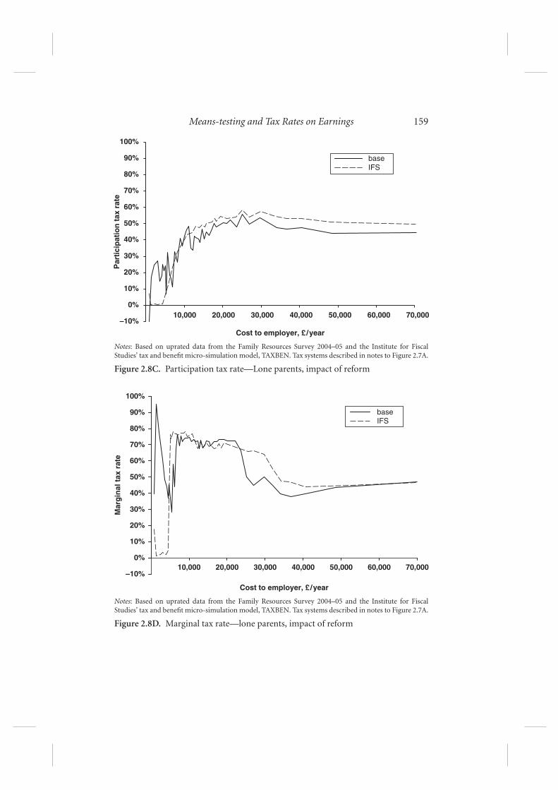
Means-testing and Tax Rates on Earnings 159
-10%
0%10,000 20,000 30,000 40,000 50,000 60,000 70,000
10%
20%
30%
40%
50%
60%
70%
80%
90%
100%
Cost to employer, £/year
Par
tici
pat
ion
tax
rat
e
baseIFS
Notes: Based on uprated data from the Family Resources Survey 2004–05 and the Institute for FiscalStudies’ tax and benefit micro-simulation model, TAXBEN. Tax systems described in notes to Figure 2.7A.
Figure 2.8C. Participation tax rate—Lone parents, impact of reform
0%10,000 20,000 30,000 40,000 50,000 60,000 70,000
10%
–10%
20%
30%
40%
50%
60%
70%
80%
90%
100%
Cost to employer, £/year
Mar
gin
al t
ax r
ate
baseIFS
Notes: Based on uprated data from the Family Resources Survey 2004–05 and the Institute for FiscalStudies’ tax and benefit micro-simulation model, TAXBEN. Tax systems described in notes to Figure 2.7A.
Figure 2.8D. Marginal tax rate—lone parents, impact of reform

160 Mike Brewer, Emmanuel Saez, and Andrew Shephard
-10%
0%10,000 20,000 30,000 40,000 50,000 60,000 70,000
10%
20%
30%
40%
50%
60%
70%
80%
90%
100%
Cost to employer, £/year
Par
tici
pat
ion
tax
rat
e
base: partner doesn't work
base: partner works
IFS: partner doesn't work
IFS: partner works
Notes: Based on uprated data from the Family Resources Survey 2004–05 and the Institute for FiscalStudies’ tax and benefit micro-simulation model, TAXBEN. Tax systems described in notes to Figure 2.7A.
Figure 2.8E. Participation tax rate—Couples no children, impact of reform
0%0 10,000 20,000 30,000 40,000 50,000 60,000 70,000
10%
20%
30%
40%
50%
60%
70%
80%
90%
100%
Cost to employer, £/year
Mar
gin
al t
ax r
ate
base: partner doesn't work
base: partner works
IFS: partner doesn't work
IFS: partner works
Notes: Based on uprated data from the Family Resources Survey 2004–05 and the Institute for FiscalStudies’ tax and benefit micro-simulation model, TAXBEN. Tax systems described in notes to Figure 2.7A.
Figure 2.8F. Marginal tax rate—Couples no children, impact of reform

Means-testing and Tax Rates on Earnings 161
-10%
0%10,000 20,000 30,000 40,000 50,000 60,000 70,000
10%
20%
30%
40%
50%
60%
70%
80%
90%
100%
Cost to employer, £/year
Par
tici
pat
ion
tax
rat
e
base: partner doesn't work
base: partner works
IFS: partner doesn't work
IFS: partner works
Notes: Based on uprated data from the Family Resources Survey 2004–05 and the Institute for FiscalStudies’ tax and benefit micro-simulation model, TAXBEN. Tax systems described in notes to Figure 2.7A.
Figure 2.8G. Participation tax rate—Couples with children, impact of reform
0%0 10,000 20,000 30,000 40,000 50,000 60,000 70,000
10%
20%
30%
40%
50%
60%
70%
80%
90%
100%
Cost to employer, £/year
Mar
gin
al t
ax r
ate
base: partner doesn't work
base: partner works
IFS: partner doesn't work
IFS: partner works
Notes: Based on uprated data from the Family Resources Survey 2004–05 and the Institute for FiscalStudies’ tax and benefit micro-simulation model, TAXBEN. Tax systems described in notes to Figure 2.7A.
Figure 2.8H. Marginal tax rate—Couples with children, impact of reform

162 Mike Brewer, Emmanuel Saez, and Andrew Shephard
rises in METRs because more of these adults are affected by the withdrawalof the IFS than are currently affected by a withdrawal of tax credits (forsingle adults without children, this is predominantly because many more areentitled to the IFS as it has no hours of work limits; for second earners incouples with children, it is predominantly because the lower IFS withdrawalrate means that its withdrawal extends further up the (family) earningsdistribution).
The online appendix (see footnote 14) explains how simple estimates ofthe behavioural response to the IFS affect the cost to the Exchequer, employ-ment, and total hours worked (or total earnings). These show that, givenreasonable assumptions on the size of behavioural responses, the impact ofthe IFS reform on the Exchequer is small but negative. The IFS reform wouldbe expected to lead to more people participating in the labour market, butaverage earnings conditional on participation falls, with the overall effect ontotal earnings being negative.71
Part of the reason for this negative behavioural response is that we havetried to reduce the generosity of the system for those with no private incomeby relatively small amounts, and we have made no cuts at all in the generosityof HB/CTB. If those programmes were made less generous to those withno private income, then income tax rates could be lowered, and the overallimpact of the IFS would be to increase total earnings. However, with the ratesproposed here, the achievement of the IFS is that it manages to redistributemore income with minimal impact on total earnings and total net tax rev-enue, by targeting net tax cuts where incentives to work are currently at theirweakest.
2.8. CONCLUSION
This chapter has provided an overview of the lessons that have been learnedover the last thirty years in the economics literature for the optimal design
71 It is not possible to estimate the impact of the behavioural responses on relative povertyrates, because the behavioural responses are modelled at an individual level. But it is possible tosay something for single adult families. For lone parents, using a calibrated poverty line so that21% of children were in relative poverty in the base system, 41% of children with lone parentswere in poverty. Before behavioural responses, this falls to 40% (70% for children with a worklesslone parent, 7% for children with a working lone parent, with 48% of children having a workinglone parent). The estimated impact of behavioural responses is to increase the number of childrenwith a working lone parent by 3.4 ppts, and to cut the poverty rate of children with working loneparents to 5%. Together, this makes the poverty rate for all children in lone parent families equalto 38%.

Means-testing and Tax Rates on Earnings 163
of household tax and benefits, and an application to the UK. We derivedformulae for the optimal tax rates using the simple Mirrlees model, andshowed the result of simulations of the whole tax system based on the UKearnings distribution and empirically estimated labour supply elasticities.We investigated the link between top incomes and top marginal income taxrates since the 1960s. We discussed how the optimal tax system is affectedby allowing for participation responses, migration, and how families andchildren should be treated.
These insights from optimal tax theory were contrasted with the workincentives inherent in the current UK tax and benefit system, and it is worthrepeating our conclusions.
First, participation tax rates at low earnings are high: for most groups, theyare close to 100% for jobs of too few hours to grant individuals entitlementto the working tax credit, and they remain high even with it. Secondly, thephasing-out of the working and child tax credits, which operates on top ofNational Insurance and income tax, generates METRs of 73.4% (includingemployer NICs) for a large number of low to moderate earners which is likelyto be above the optimal rate even with modest behavioural responses. Third,the main means-tested programme to help with housing (housing benefit)has an extremely high withdrawal rate (further increasing METRs), admin-istrative difficulties, and problems of misperception which deter low-incomeworking families from claiming it. Finally, while the system for administeringincome tax and NICs in the UK is simple and efficient, the systems for admin-istering child and working tax credits, and for housing benefit and council taxbenefit, are administratively burdensome for claimants, relatively expensivefor the government, and prone to large amounts of fraud and error: all meanthat neither are as well-targeted on the economic situation of beneficiaries asthey could be.
Given this, we suggest a set of changes to the existing tax and benefitstructure that could be made immediately based on the lessons from ouranalysis. Our package of ‘immediate reforms’ is costly, and involves increasingthe level of earnings disregards in all of the means-tested benefits to reducePTRs on low earnings and introducing an additional earnings disregard intax credits for second earners to reduce PTRs for secondary earners, par-ticularly those with children. Work incentives can be further improved byreductions in the withdrawal rate in child and working tax credits, andby targeting increases in the working tax credit on groups other than loneparents.
We also provide a more radical and comprehensive plan for reforming theUK household tax and benefit system that attempts to deal not only with these

164 Mike Brewer, Emmanuel Saez, and Andrew Shephard
work incentive issues, but also the administrative failings that we identify.Our plan replaces the piecemeal benefits for low-income families (incomesupport, working and child tax credits, housing benefit, and council taxbenefit) into a single Integrated Family Support programme which providesstronger and simpler incentives for work at the bottom, reduces compliancecosts for families, and is provided ‘as-you-earn’ and administered in the sameway as NICs through the PAYE withholding system. We show how this can bedone in a revenue-neutral fashion, including an assessment of the behaviouralresponses. The key achievement of the IFS is that it manages to redistributeincome with minimal impact on total earnings and total net tax revenue, bytargeting net tax cuts which work with the grain, rather than against the grain,of individuals’ work incentives.
We have used the framework of optimal tax theory to guide our discussionthroughout this chapter. We argued that one attractive feature of this theoryis that it makes explicit that one cannot hope to say how best to design taxesand transfers without specifying what one is trying to achieve overall. This,of course, may prove to be our ultimate downfall. Without knowing thegovernment’s preferences for redistribution or other objectives, we cannothope to predict whether our reform will appeal.
APPENDIX
This appendix provides a more formal discussion of the derivation of optimal incometax rates. We first show how to determine the optimal marginal tax rate for highearners, and then how to derive optimal tax rates for taxpayers more generally.
2A.1. Determining the top rate of income tax
Consider a reform that changes the top tax rate Ù by a small amount dÙ (with nochange in the tax schedule for incomes below the top bracket z). Here, let us denoteby z the average income reported by taxpayers in the top bracket and let us assumethat there are N taxpayers in the top bracket. As mentioned in the main text, thissmall tax reform has the following effects on tax revenue:
1. There is a mechanical increase in tax revenue because taxpayers face a higherMTR on incomes above z. Hence, the total mechanical effect is d M = N[z −z]dÙ > 0. This mechanical effect is the projected increase in tax revenue if therewere no behavioural response.

Means-testing and Tax Rates on Earnings 165
2. The increase in the tax rate triggers a behavioural response which reducesthe average reported income in the top bracket by dz = −e · z · dÙ/(1 − Ù) onaverage (by definition of the elasticity e—see Box 2.1 in Section 2.2) and henceproduces a loss in tax revenue equal to d B = −N · e · z · dÙ · Ù/(1 − Ù) < 0.
Rather than necessarily assuming that the marginal value of consumption for toptaxpayers is negligible relative to that of the average person in the economy, let usassume that the government values giving one additional pound to the average topbracket taxpayer at g . If the government values redistribution, g will be strictly lessthan one, and will be zero if the government has strong redistributive tastes (the caseconsidered in the main text). Hence, the small tax reform also creates a social welfarecost equal to dW = −g · N [z − z] dÙ < 0.
Summing the mechanical and the behavioural tax revenue effect and the welfareeffect, we obtain the net effect of the reform from the government perspective:
d M + d B + dW = NdÙ(z − z) ·[
1 − g − e · z
z − z· Ù
1 − Ù
]
At the optimum, this expression must be zero. As before, let us denote by a the ratioz/(z − z), which measures the thinness of the top of the income distribution. Notethat a � 1. The optimal Ù can then be expressed as:
Ù∗ =1 − g
1 − g + a · e. (1)
Unsurprisingly, the optimal tax rate is decreasing in g (the value that the govern-ment sets on the marginal consumption of high incomes), decreasing in the elasticitye of behavioural responses, and decreasing in a , the parameter which measures thethinness of the top of the income distribution. Note that this expression is identical tothat presented in Box 2.2 when g = 0. This important case gives an upper bound onthe optimal top rate equal to 1/(1 + a · e). This corresponds to the tax rate maximiz-ing tax revenue from top bracket taxpayers: the so-called Laffer rate. Finally, we notethat it is well known that top tails of income distributions are closely approximatedby Pareto distributions,72 in which case the parameter a does not vary with z and isexactly equal to the Pareto parameter.73
72 A Pareto distribution has a density function of the form f (z) = C/z1+· where C and · areconstant parameters. · is called the Pareto parameter.
73 When z reaches the level of the very highest income earner, z = z and a is infinite and theoptimal tax rate is zero, which is the famous Sadka–Seade zero top result. However, this zero topresult is a very misleading result for practical tax policy as the empirical a does not go to infinityexcept for the very highest income earner.

166 Mike Brewer, Emmanuel Saez, and Andrew Shephard
2A.2. Determining the optimal marginal tax schedules
We can extend the above analysis to consider how the optimal tax rate varies moregenerally across the income distribution. Here, we let T(z) denote the (possibly non-linear) tax schedule that the government imposes, where z denotes a given level ofearnings. This tax schedule incorporates both transfers (when T(z) is negative) andtaxes (when T(z) is positive). Let us denote by H(z) the cumulative distribution ofindividuals (fraction of taxpayers with income less than z) and by h(z) the densitydistribution of taxpayers. The optimal tax system is characterized by a lump-sumgrant received by those with no earnings (equal to −T(0)) combined with a scheduleof marginal tax rates T ′(z) which define how the lump-sum grant should be reducedas earnings increase and how additional earnings should be taxed once the lump-sum grant is fully tapered out. Again, the optimal marginal tax rate T ′(z) is set so asto balance costs and benefits at the margin.
Suppose that the government increases the marginal tax rate T ′(z) by dÙ in a smallband of income (z, z + dz). As above, this reform has three effects on government taxreceipts and welfare:
1. The reform increases taxes by dÙdz for every taxpayer above the small band,and hence collects extra taxes d M = (1 − H(z))dÙdz.
2. Those extra taxes generate a welfare cost to taxpayers. If we denote by G(z) theaverage social value for the government of distributing £1 uniformly amongtaxpayers with income above z, the welfare cost is simply dW = d M · G(z).74 Ifthe government values redistribution, G(z) will be decreasing in z. As we haveassumed away income effects, G(0) = 1,75 and we assumed above that G(z)goes to zero when z is large (i.e. in the top tax bracket). The more redistributivethe tastes of the government, the smaller G(z).
3. The marginal tax rate increase dÙ in the small band reduces earnings by−e · z · dÙ/(1 − T ′(z)) for taxpayers in the small band due to the substitutioneffect. There are h(z)dz such taxpayers in the small band, and so this producesa loss in tax revenue equal to d B = −e · z · [
T ′(z)/(1 − T ′(z))]
dÙ · h(z)dz.
At the optimum, d M + dW + d B = 0, which generates the following optimal taxrate formula:76
T ′(z)
1 − T ′(z)=
1
e· 1 − H(z)
zh(z)· (1 − G(z)).
74 This is a consequence of the envelope theorem as each individual maximizes utility.75 Distributing £1 uniformly among all individuals does not generate behavioural responses and
hence has a cost of exactly £1 for the government.76 This formula is not exactly accurate but very close for discussion and intuition purposes. In
the exact formula, h(z) should be replaced with the ‘virtual’ density h∗(z), which is the density ofearnings at z that would arise if the tax system were replaced by the linearized tax system at z. SeeSaez (2001) for complete details.

Means-testing and Tax Rates on Earnings 167
The optimal tax rate T ′(z) is decreasing with the elasticity e . It is also decreasingin G(z) which measures the social marginal value of consumption for individualswith earnings above z, and decreasing in the hazard ratio (1 − H(z))/(zh(z)) whichmeasures the thinness of the distribution.
2A.3. Optimal tax rates with participation responses
Here, an individual with skill z who decides to work will get z − T(z) in disposableincome. If the individual decides not to work, she will get −T(0) in disposableincome. We assume that individual utility is simply u = c − q where c is disposableincome and q are costs of work. Hence, the individual will work if the net return towork z − T(z) + T(0) exceeds her costs of working q . If we assume that costs of workq are distributed with a (cumulative) distribution P (q |z) among individuals withskill z, the number of individuals of skill z who work is simply P (z − T(z) + T(0)|z).We can define the elasticity of participation with respect to the net return to work as:
Á(z) =z − T(z) + T(0)
P· ∂ P
∂q. (2)
To derive an optimal tax formula, let us consider a small increase in dT in T(z)but only at skill level z. As there are only extensive responses, this reform affects onlyindividuals with skill z. As above, this reform has three effects on government taxreceipts and welfare:
1. The reform increases taxes by dT for every taxpayer with skill z who works andhence collects extra taxes d M = P (q |z)dT .
2. The extra taxes that are now collected generate a welfare cost to workerswith skill z. If we denote by g (z) the social value for the government ofdistributing £1 among taxpayers with income z, the welfare cost is simplydW = d M · g (z) = P (q |z)g (z)dT . If the government values redistribution,g (z) will be decreasing in z. The ‘no income effect’ assumption implies thatthe average g (z) across the population is equal to one. Note that the g (z) ofthis section and the G(z) of the previous section are related by the formulaG(z)(1 − H(z)) =
∫ ∞z g (z)h(z)dz.
3. The tax increase dT at income level z induces some of the workers at z todrop out of work. All those with fixed cost of work q between z − T(z) +T(0) − dT and z − T(z) + T(0) drop out. There are dT∂ P/∂q = dTÁP/(z −T(z) + T(0)) such workers. The fiscal cost of this behavioural response isd B = [(T(z) − T(0))/(z − T(z) + T(0))] · Á · P (q |z)dT .77
77 Note that those dropping out of the labour force are indifferent (within dT) between workingand not working and there is only an infinitesimal number of switchers. Hence the welfare effect onmovers is second order relative to the welfare effect on those who work and can be neglected. Thisis directly equivalent to the situation from Section 2.2 where behavioural responses do not create afirst-order welfare effect.

168 Mike Brewer, Emmanuel Saez, and Andrew Shephard
To proceed, define the participation tax rate, a measure of the extent to which thetax and benefit system weakens the reward from working, as t(z) = (T(z) − T(0))/z.As discussed above, 1 − t(z) measures the increase in disposable income (relative toearnings) when an individual decides to work. Using this definition, and noting thatat the optimum we again must have d M + dW + d B = 0, we generate the followingoptimal tax rate formula:
t(z)
1 − t(z)=
1
Á· (1 − g (z)). (3)
This formula is a simple inverse elasticity tax rule for the average tax rate on work.The average tax rate decreases with the elasticity Á and also decreases with g (z), thesocial value of marginal consumption for individuals earning z.
REFERENCES
Aaberge, R., Colombino, U., and Strøm, S. (1999), ‘Labor Supply in Italy: An Empir-ical Analysis of Joint Household Decisions, with Taxes and Quantity Constraints’,Journal of Applied Econometrics, 14, 403–22.
Adam, S. (2005), ‘Measuring the Marginal Efficiency Cost of Redistribution in theUK’, IFS Working Paper, W05/14.
—— and Brewer, M. (2004), Supporting Families: The Financial Costs and Benefits ofChildren since 1975, Bristol: The Policy Press.
—— —— and Shephard, A. (2006), The Poverty Trade-off: Work Incentives andIncome Redistribution in Britain, Bristol: The Policy Press.
—— —— Browne, J., and Phillips, D. (2007), ‘Government Financial Support forChildren across the United Kingdom: How does Northern Ireland Compare?’,Belfast: NICCY.
—— Emmerson, C., and Kenley, A. (2007), ‘A Survey of UK Local GovernmentFinance’, IFS Briefing Note 74, http://www.ifs.org.uk/bns/bn74.pdf.
Adda, J., Dustmann, C., Meghir, C., and Robin, J-M. (2006), ‘Career Progression andFormal versus On-the-Job Training’, IZA Discussion Papers 2260, Institute for theStudy of Labor (IZA).
Akerlof, G. A. (1978), ‘The Economics of “Tagging” as Applied to the OptimalIncome Tax, Welfare Programs, and Manpower Planning’, The American EconomicReview, 68, 8–19.
Alesina, A., and Ichino, A. (2007), ‘Gender based taxation’, Harvard University Work-ing Paper, April.
Anderberg, D., Kondylis, F., and Walker, I. (2008), ‘Partnership Penalties and BonusesCreated by UK Welfare Programs’, CESifo Economic Studies, 54, 1–21.

Means-testing and Tax Rates on Earnings 169
Arrufat, J., and Zabalza, A. (1986), ‘Female Labor Supply with Taxation, RandomPreferences, and Optimization Errors’, Econometrica, 54, 47–64.
Atkinson, A. (2007), ‘Top Incomes in the United Kingdom over the TwentiethCentury’, in Atkinson, A. and Piketty, T. eds., Top Incomes from a Historical andInternational Perspective, 89, Oxford: Oxford University Press.
—— and Leigh, A. (2004), ‘Understanding the Distribution of Top Incomesin Anglo-Saxon Countries over the Twentieth Century’, Department ofEconomics, Australian National University. http://cepr.anu.edu.au/∼aleigh/pdf/TopIncomesAnglo.pdf.
Baughman, R., and Dickert-Conlin, S. (2003), ‘Did Expanding the EITC PromoteMotherhood?’, American Economic Review, American Economic Association, 93,May, 247–51.
Bell, K., Brewer, M., and Phillips, D. (2007), ‘Lone Parents and Mini Jobs’, York: YPS.Blow, L., and Preston, I. (2002), ‘Deadweight Loss and Taxation of Earned Income:
Evidence from Tax Records of the UK Self-Employed’, IFS Working PaperNo. 02/15.
Blundell, R., Chiappori, P.-A., and C. Meghir, (2005), ‘Collective Labor Supply withChildren’, Journal of Political Economy, 113, 1277–306.
—— and MaCurdy, T. (1999), ‘Labour Supply: A Review of Alternative Approaches’,in Ashenfelter, O., and Card, D. (eds.), Handbook of Labour Economics, vol. 3A,Amsterdam: North-Holland.
—— and Shephard, A. (2008), ‘Employment, Hours of Work and the OptimalDesign of Earned Income Tax Credits’, IFS Working Paper W08/01.
Boskin, M., and Eytan, S. (1983), ‘Optimal Tax Treatment of the Family: MarriedCouples’, Journal of Public Economics, 20, 281–97.
Bowler, T. (2007), ‘Taxation of the Family’, TLRC Discussion Paper 6, http://www.ifs.org.uk/comms/dp6.pdf, London: IFS.
Brewer, M. (2006), ‘Tax Credits Fixed or Beyond Repair?’, in Chote, R. Emmerson, C.Harrison, R., and Miles, D. eds., The IFS Green Budget 2006, London: IFS.
—— (2007), ‘Supporting Couples with Children Through the Tax System’, in Chote,R., Emmerson, C., Leicester, A., and Miles, D., eds., The IFS Green Budget 2007,London: IFS.
—— Browne, J., Emmerson, C., Goodman, A., Muriel, A., and Tetlow, G. (2007a),Pensioner Poverty Over the Next Decade: What Role for Tax and Benefit Reform?,Commentary 103, London: IFS.
—— Clark, T., and Myck, M. (2001), ‘Credit where it’s Due? An Assessment of theNew Tax Credits’, IFS Commentary 86, London: IFS. doi: 10.1920/co.ifs.2001.0086.
—— Duncan, A., Shephard, A., and Suarez, M. J. (2006), ‘Did Working Families’ TaxCredit Work? The Impact of In-work Support on Labour Supply in Great Britain’,Labour Economics, 13, 699–720.
—— Muriel, A., Phillips, D., and Sibieta, L. (2008b), ‘Poverty and Inequality in theUK: 2008’, IFS Commentary 105, London. IFS: doi: 10.1920/co.ifs.2008.0105.

170 Mike Brewer, Emmanuel Saez, and Andrew Shephard
Brewer, M., Ratcliffe, A., and Smith, S. (2007b), ‘Does Welfare Reform Affect Fertility?Evidence from the UK’, CMPO Working Paper 07/177.
—— and Shaw, J. (2006), ‘How Many Lone Parents are Receiving Tax Credits?’,Institute for Fiscal Studies Briefing Note 70.
—— Sibieta, L., and Wren-Lewis, L. (2008a), ‘Racing Away? Income Inequalityand the Evolution of High Incomes’, IFS Briefing Notes, BN76, doi: 10.1920/bn.ifs.2008.0076.
Chiappori, P.-A. (1988), ‘Rational Household Labour Supply’, Econometrica, 56,63–90.
—— (1992), ‘Collective Labour Supply and Welfare’, Journal of Political Economy,100, 437–67.
Cm 6951 (2006–07), (2006), Delivering on Child Poverty: What Would it Take?,A report for the Department for Work and Pensions, Cm 6951, November2006.
Cm 6983, (2006–07), HM Revenue and Customs Annual Report 2005–06, London:The Stationery Office.
Cm 7130 (2006–07), In Work, Better Off, London: TSO.Cm 7290 (2006–07), Ready for Work: Full Employment in our Generation, London:
TSO.Community Links, Low Incomes Tax Reform Group and Child Poverty Action
Group (2007), ‘Interact: Benefits, Tax Credits and Moving into Work’, London:Community Links, Low Incomes Tax Reform Group and Child Poverty ActionGroup.
Cooke, G., and Lawton, K. (2008) ‘Working out of Poverty: A Study of the LowPaid and the “Working Poor” ’, <http://www.ippr.org/publicationsandreports/publication.asp?id=581>.
DWP (2007a), ‘Fraud and Error in the Benefit System April 2005 to March 2006’,<http://www.dwp.gov.uk/asd/asd2/fem/fem_apr05_mar06.pdf>.
Devereux, P. J. (2004), ‘Changes in Relative Wages and Family Labor Supply’, Journalof Human Resources, 39, 696–722.
Di Tommaso, M. L., Dex, S., and Rowthorn, R. E. (1999), ‘Women’s Labour SupplyDecisions in the Light of Possible Fiscal Reforms’, Research Paper WP36/99, Uni-versity of Cambridge: Judge Institute of Management.
Diamond, P. (1980), ‘Income Taxation with Fixed Hours of Work,’ Journal of PublicEconomics, 13, 101–10.
—— (1998), ‘Optimal Income Taxation: An Example with a U-Shaped Pattern ofOptimal Marginal Tax Rates’, American Economic Review, 88, 83–95.
Dilnot, A., Kay, J., and Morris, N. (1984), The Reform of Social Security, Oxford:Clarendon Press.
—— and Kell, M. (1988), ‘Top-Rate Tax Cuts and Incentives: Some Empirical Evi-dence’, Fiscal Studies, 9, 70–92.
Draper, D. (2007), ‘Families Compared 2006/7’, CARE Research Paper, <http://www.care.org.uk/Publisher/File.aspx?ID=13022>.

Means-testing and Tax Rates on Earnings 171
Eissa, N., and Hognes, H. (2000), ‘Explaining the Fall and Rise in the Tax Cost ofMarriage: The Effect of Tax Laws and Demographic Trends, 1984–1997’. NationalTax Journal, 53, 683–711.
—— —— (2004), ‘Taxes and the Labor Market Participation of Married Couples:The Earned Income Tax Credit’, Journal of Public Economics, 88, 1931–58.
Gentry, W. R., and Hubbard, R. G. (2004), ‘Success Taxes, Entrepreneurial Entry, andInnovation’, NBER Working Paper No. 10551.
Griffith, R., and Klemm, A. (2004), ‘What has been the Tax Competition Experienceof the last 20 Years?’, Tax Notes International, 34, 1299–316.
Gruber, J., and Saez, E., (2002), ‘The Elasticity of Taxable Income: Evidence andImplications’, Journal of Public Economics, 84, 1–32.
Guesnerie, R. and Roberts, K. (1984), ‘Effective Policy Tools and Quantity Controls’,Econometrica, 52, 59–86.
Heim, B. T. and Meyer, B. (2004), ‘Work Costs and Nonconvex Preferences in theEstimation of Labour Supply Models’, Journal of Public Economics, 88, 2323–38.
Hills, J., McKnight, A., and Smithies, R. (2006), ‘Tracking Income: How WorkingFamilies’ Incomes Vary Through the Year’, CASE report 32, London: CASE/LSE.
HC 32 (2007–08), ‘Sustainable Employment: Supporting People to Stay in Work andAdvance’, London: TSO.
HC 42-I (2007–08), ‘The Best Start in Life? Alleviating Deprivation, Improving SocialMobility and Eradicating Child Poverty’, London: TSO.
HC 609 (2006–07), ‘Helping People from Workless Households into Work’, London:TSO.
HC 626 (2006–07), ‘HM Revenue and Customs 2006–07 Accounts: The Comptrollerand Auditor General’s Standard Report’, London: TSO.
HC 1010 (2006–07), ‘Tax Credits: Getting it Wrong’, London: TSO.HMRC (2007), ‘Child Tax Credit and Working Tax Credit Take-up rates 2004–05’,
<http://www.hmrc.gov.uk/stats/personal-tax-credits/takeup-rates2004-05.pdf>.HMRC (2007b), ‘Child and Working Tax Credits: Error and Fraud statistics,
2004–05’, <http://www.hmrc.gov.uk/stats/personal-tax-credits/cwtc-error0405.pdf>.
HMRC (2007c), ‘Number of Individual Income Taxpayers’, <http://www.hmrc.gov.uk/stats/income_tax/table2-1.pdf>.
Hotz, V. J., and Scholz, J. K. (2003), ‘The Earned Income Tax Credit’, in Moffitt,R., ed., Means-Tested Transfer programmes in the U.S., Chicago: University ofChicago Press.
Hoynes, H. (1997), ‘Work, Welfare and Family Structure’, in Auerbach, A. (ed.), FiscalPolicy: Lessons from Economic Research.
Immervoll, H., Kleven, H., Kreiner, C., and Saez, E. (2007), ‘Welfare Reform inEuropean Countries: Microsimulation Analysis’, Economic Journal, 117,1–44.
Kanbur, R., Keen, M., and Tuomala, M. (1994), ‘Optimal Non-linear Income Tax-ation for the Alleviation of Income-Poverty’, European Economic Review, 38,1613–32.

172 Mike Brewer, Emmanuel Saez, and Andrew Shephard
Kirby, J. (2005), The Price of Parenthood, London: Centre for Policy Studies.Kleven, H., Kreiner, C., and Saez, E. (2006), ‘The Optimal Taxation of Couples’, NBER
Working Paper No. 12685.Kluve, J., Card, D., Fertig, M., Góra, M., Jacobi, L., Jensen, P., Leetmaa, R., Nima,
L., Patacchini, E., Schaffner, S., Schmidt, C. M., van der Klaauw, B., and Weber, A.(2007), Active Labor Market Policy in Europe: Performance and Perspectives, Berlinet al.: Springer.
Laroque, G., and Salanié, B. (2005), ‘Fertility and Financial Incentives in France’,CESIfo Economic Studies, 50, 423–50.
Lundberg, S. J., Pollak, R. A., and Wales, T. J. (1997), ‘Do Husbands and Wives PoolTheir Resources: Evidence from the United Kingdom Child Tax Credit’, Journal ofHuman Resources, 32, 463–80.
Meade, J. (1978), The Structure and Reform of Direct Taxation: Report of a Committeechaired by Professor J. E. Meade for the Institute for Fiscal Studies, London: GeorgeAllen & Unwin. http://www.ifs.org.uk/publications/3433.
Milligan, K. (2005), ‘Subsidizing the Stork: New Evidence on Tax Incentives andFertility’, Review of Economics and Statistics, 87, 539–55.
Mirrlees, J. (1971), ‘An Exploration in the Theory of Optimal Income Taxation’,Review of Economic Studies, 38, 175–208.
—— (1982), ‘Migration and Optimal Income Taxes’, Journal of Public Economics, 18,319–41.
Moffitt, R. (2006), ‘Welfare Work Requirements with Paternalistic Government Pref-erences’, Economic Journal, 116, F441–F458.
O’Dea, C., Phillips, D., and Vink, A. (2007), ‘A Survey of the UK Benefit System’,Institute for Fiscal Studies Briefing Note 13.
Pencavel, J. (1986), ‘Labor Supply of Men: A Survey’, in Ashenfelter, O.,and Layard, R. (eds.), Handbook of Labor Economics, 1, 3–102. Amsterdam:North-Holland.
Piketty, T., and Saez, E. (2007), ‘How Progressive is the U.S. Federal Tax System?A Historical and International Perspective’, Journal of Economic Perspectives, 21,3–24.
Saez, E. (2001), ‘Using Elasticities to Derive Optimal Income Tax Rates’, Review ofEconomic Studies, 68, 205–29.
—— (2002a), ‘Optimal Income Transfer programmes: Intensive Versus Extensivelabour Supply Responses’, Quarterly Journal of Economics, 117, 1039–73.
—— (2002b), ‘Do Taxpayers Bunch at Kink Points?’, NBER Working PaperNo. 7366.
—— (2004), ‘Reported Incomes and Marginal Tax Rates, 1960–2000: Evidenceand Policy Implications’, in Poterba, J. (ed.), Tax Policy and the Economy,18, 117–74.
Simula, L. and Trannoy, A. (2006), ‘Optimal Non-Linear Income Tax when AgentsVote with their Feet’, Finanzarchiv, 62, 393–415.

Means-testing and Tax Rates on Earnings 173
Social Justice Policy Group (2007), Breakthrough Britain, London: Social JusticePolicy Group.
Turley, C., and Thomas, A. (2006), Housing Benefit and Council Tax Benefit as In-work Benefits; Claimants’ and Advisors’ Knowledge, Attitudes and Experiences, DWPResearch Report 383, Leeds: CDS.
Whiteford, P., Mendelson, M., and Millar, J. (2003), Timing it Right? Tax Credits andhow to Respond to Income Changes, York: JRF.

© Institute for Fiscal Studies, 2009
1
Means-testing and tax rates on earnings: on-line
appendix
Mike Brewer, Emmanuel Saez and Andrew Shephard
January 2010
This document provides supplementary material to the chapter “Means-
testing and tax rates on earnings”, due to published in Dimensions of Tax
Design by OUP in 2010. A draft version is also available at
http://www.ifs.org.uk/mirrleesreview/press_docs/rates.pdf.
Figures 2.2A and 2.2B use data on top income shares in the UK, and on
METRs affecting individuals with high incomes, which uses data on top
income levels. This section details how they were constructed.
The series on top income shares and levels was taken from Atkinson
(2007) and updated by the authors to include 2001/2 - 2004/5 using the
Survey of Personal Incomes, and with total adult population in those years
taken from Population Trends. It did not prove possible to replicate the
series for total income given in Atkinson (2007) for years up to 2000, and
so total income in 2001/2 to 2003/4 was assumed to grow at the same
rate as SPI income grew for those years, and these used to estimate top
income shares.
The Atkinson series display a discontinuity from 1989 to 1990 due to the
shift from family-based income taxation to individual-based income
taxation. In order to smooth the series, we have uniformly increased all the
top share series by 5% for years 1962 to 1989. This increase
approximately smooths the income share series around the 1989-1990
change.
METRs applying to top incomes over time were calculated by the authors.
For years 1975/6 - 2004/5, the calculation used TAXBEN, the IFS' tax and
benefit microsimulation model. For previous years, they were based on the
authors' understanding of the tax system drawing on an unpublished
document produced by HM Treasury called “A Guide to the Tax and Benefit
System”. Data from Atkinson (2007) and updated by the authors to include

© Institute for Fiscal Studies, 2009
2
2001/2 - 2004/5 using the Survey of Personal Incomes were used to
estimate what share of top incomes were from earnings, self-employment,
investment and other sources, and it was assumed that the marginal
pound was split between these sources identically to the average pound.
All individuals are assumed to be a single-earner couple with two children
(family status and the presence of and number of dependent children
affects tax liability in some, but not all, years under consideration). For
years after 1984, METRs on earned income include employer NI, and, for
2003/4 and 2004/5, employee NI.
The optimal Mirrlees tax simulations proceed as follows. We assume that
individuals differ only in their ability n. The utility function takes the
following quasi-linear and iso-elastic form:
where c is disposable after tax and transfer income available for
consumption, z is earnings, and e is a positive constant parameter. u is
increasing in c and decreasing in z, as earnings requires labour supply.
With a nonlinear income tax, c=z-T(z) and each individual chooses z to
maximize . The first order condition for z is
, which can be rewritten as
Hence e is the elasticity of reported earnings with respect to the net-of-tax
rate . As there are no income effects, this elasticity is both the
compensated and uncompensated elasticity. Note that with no marginal
tax, z=n so that ability n represents undistorted potential earnings. We
assume that n has a distribution F(n) with density f(n). We normalize the
total population to one.
We estimate f(n) based on the actual earnings distribution as follows.
Denote by H0(z0) the actual distribution of annual earnings among all
individuals in the UK of working age. This distribution is obtained from
merging the Family Resources Survey data (for those with earnings below
£60,000) and the individual income tax returns (from the Survey of
Personal Incomes for those with earnings above £60,000). We assume that
the distribution of earnings above £300,000 follows a Pareto distribution

© Institute for Fiscal Studies, 2009
3
with parameter a=1.6. Earnings are defined as the sum of wages (inclusive
of employee and employer payroll taxes) and self employment earnings.
For each individual, we estimate the corresponding marginal tax rate using
the TAXBEN micro-simulation model, where we include in the marginal
tax computation the individual income tax, the payroll taxes (both
employee and employer), the main transfers for low income earners
(including housing benefit, council tax benefit, income support and in-
work tax credits), and a flat value added tax (equal to 17.2%: this is the
ratio of VAT collected divided by total consumption from National
Accounts).
We then estimate potential earnings n for an individual with earnings z
and facing an actual marginal tax rate T’ as (using the
equation above, and given a value of e). This allows us to obtain a
distribution of potential earnings n. We smooth the distribution of
potential earnings f(n) to obtain a smooth schedule of optimal tax rates.
We assume that the government maximizes:
subject to the budget constraint
where E is government spending (excluding redistributive transfers) and γ
measures the strength of the redistributive tastes of the government. In
the simulations, we assume that E is equal to average tax revenue net of
transfers. Specifically, the revenue requirement is calculated by adding
together total household income tax receipts, total (employees',
employers', and self-employed persons') national insurance contributions,
and consumption tax revenue. Consumption tax revenue is calculated by
aggregating all product taxes from National Accounts and scaling by the
proportion of non-pensioners in the total population. From this we deduct
expenditure on Job Seekers Allowance, income tax credits and reliefs,
child benefit, housing benefit, council tax benefit and income support that
are received by the working-age population (using expenditure figures
from the Department for Work and Pensions). We then divide by the total
working-age population to calculate the revenue requirement E. Hence our

© Institute for Fiscal Studies, 2009
4
optimal tax system keeps government spending (outside of direct
redistribution) constant.
In our simple model, the optimal Mirrlees formula takes the following
form:
where is the multiplier of the budget constraint. The transversality
condition implies that:
We select a (log) grid for n, from 1 to 10^6, with 2,000 elements.
Integration along the n variable is carried out using the trapezoidal
approximation in Matlab.
We start with a given T’, and then derive all the vector variables z, u, T, ,
etc. which satisfy the government’s budget constraint and the
transversality conditions. We adjust the constants for T(0) until all those
constraints are satisfied. This is done using a secondary iterative
procedure. We then use the first order condition to compute a new vector
T’. We then repeat the algorithm. This procedure converges to a fixed point
in most circumstances. The fixed point satisfies all the constraints and the
first order conditions. We check that the resulting z is non-decreasing so
that the fixed point is implementable, and thus the fixed point is expected
to be the optimum.
In the paper, we present simulations for two cases: e=0.25 and e=0.5. We
choose γ=1. We assume that there is an atom of non-workers (fixed by
assumption of the intensive margin model) and given by the data. The
overall METRs we obtain should replace all VAT, individual income tax,
transfers, and payroll taxes. We plot on the graphs the difference between
the optimum and the actual schedules. To facilitate discussion of reform,
we compute an income tax/transfer schedule that would be optimum if the
UK kept in place (1) the current VAT, (2) the current VAT and the current
payroll tax. This is done by assuming that (1-MTRincome) (1-MTRVAT)=(1-
MTRtotal).

© Institute for Fiscal Studies, 2009
5
Taxes and transfers might affect migration in or out of the country. For
example, high tax rates on skilled workers in continental Europe might
induce some of them to move to the UK or the US where the burden of tax
on high-income individuals may be lower, and generous benefits for
lower- income individuals in certain countries might encourage migration
of low-skilled workers toward those countries. Clearly, governments can
use other tools to affect immigration, and such policies are taken here as
given. Emigration and immigration across EU countries is almost
completely deregulated, and so our analysis is particularly relevant in this
context.
For simplicity, suppose that the only behavioral response to taxes is
migration (Mirrlees (1982) proposed such a model of optimal taxes with
migration. Simula and Trannoy (2006) propose a recent extensive
theoretical analysis of the problem). In the model presented above, one
simply needs to replace not working (and collecting transfers) by being
out of the country (and hence neither receiving transfers or paying taxes in
the domestic economy). In such a setting, we can define an elasticity of
migration with respect to disposable income as follows:
where P(c|z) is the fraction of individuals with potential earnings z which
decide to remain domestic residents when disposable domestic income is
c=z-T(z). By balancing the costs and benefits of a small tax reform at the
margin, and assuming that the government cares equally about a person
whether he or she is a domestic resident or not, we can obtain the simple
formula:
which states that the government should impose lower taxes when an
individual’s migration decision is more responsive to changes in taxes (i.e.
the migration elasticity is high).
In the EU context, the most interesting application of the tax-induced
migration model is perhaps at the high income end. If high income
© Institute for Fiscal Studies, 2009
6
individuals are able to respond to high METRs both by reducing their
effort when working, and by completely withdrawing their labour from a
given country, then the migration threat might decrease significantly the
ability of European countries to tax high incomes. As is well known, in the
presence of migration, single countries do not recognize the external cost
they might impose on others by cutting their top tax rates.1 In that case,
some form of coordination and harmonization across countries can in
principle be beneficial.
We assume that high income earners respond both along the intensive
margin with elasticity e, and along the migration margin with elasticity .
It is then possible to show that the optimal top rate maximizing tax
revenue becomes:
For example if a=2, e=0.25, the Laffer rate with no migration is 2/3. If
there is migration with =0.5, then the Laffer rate decreases to 1/2.
Thus, the possibility of migration from top earners can decrease
significantly the ability of European countries to tax high incomes.
Unfortunately, there are few empirical studies estimating the effects of tax
differentials between countries on migration. As a first step, we have
examined the basic trends in the fraction of high income earners in the
United Kingdom who are foreign-born among , and the extent to which
those trends are related to trends in the top METR. Figure 6 displays the
fraction of foreign-born workers in the top 1% and the bottom 99% from
1972 to 2004. Data from the General Household Survey (since the early
1970s) and Labour Force Survey (since 1992) records the country of birth
and Nationality of survey participants. Before 1992, our estimates are
based on the GHS which is a smaller sample than LFS. As a result, the year
to year results for the top 1% are fairly noisy and we average across 3
years. Interestingly, the fraction foreign-born increases sharply during the
1980s when METRs were falling, and only at the top of the distribution:
the fraction foreign-born in the top 1% doubles from 8% in the early

© Institute for Fiscal Studies, 2009
7
1970s to about 16% in mid-1990s, while the fraction foreign-born in the
bottom 99% stays about constant at 6-7% during the period. Since 1995,
the fraction foreign-born has increased both in the top 1% and the bottom
99%.
Figure A1. Fraction foreign born in top 1% and bottom 99% from 1972 to
2004
Notes and sources: see text for details.
If we are willing to assume (heroically) that the sharp increase in foreign
born from 8% to 16% at the top from the 1970s to 1995 was entirely due
to the drop in top tax rates, then we can provide an illustrative estimate of
the migration elasticity. According to Piketty and Saez (2007), the average
income tax rate (including income and payroll taxes) for the top 1% fell
from about 56% in 1970 to around 40% in 2000, so the net-of-tax rate
increased from 0.44 to 0.6, i.e., by 36%. The statistics from GHS and LFS
suggest that the net flow of foreigners was around 8% (an increase from
8% to 16%), and this implies a migration elasticity of 0.22. Clearly, the
flow of foreigners might have been accompanied by a flow of wealthy UK
nationals back into the UK following the tax cuts (that we cannot
measure). If that flow is comparable to the flow of foreigners, then that
would double the elasticity to 0.44. However, this analysis is extremely
0%
2%
4%
6%
8%
10%
12%
14%
16%
18%
20%
19
72
19
76
19
80
19
84
19
88
19
92
19
96
20
00
20
04
Fra
cti
on
fo
reig
n b
orn
Year
top 1%, GHS
top 1%, LFS
bottom 99%, GHS
bottom 99%, LFS

© Institute for Fiscal Studies, 2009
8
tentative: the assumption that the increase in foreigners was entirely tax-
driven is highly questionable, and was made for illustrative purposes only.
It is also important to note that the elasticity estimated from our top
income share analysis in the chapter incorporated such migration effects,
as migration to the UK of highly-skilled foreign workers will lead to a rise
in top income shares.
The maximum entitlement to the IFS would be family based, and would be
a sum of several components: a family component (different for single
adults and couples), a child component (depending on the presence and
number of dependent children), and a housing component (depending on
whether the family rents or owns, and on the local rental and council tax
levels). This maximum IFS allowance would be paid on a regular basis by
the government directly to eligible families; there would be a very strong
presumption that the child component would be sent to the mother (to
ensure that its use is more closely directed toward children, following the
analysis by Lundberg et al. (1997)) and the family and housing
components would be split between the two adults in a couple. The basic
entitlement to the IFS would not vary with the adult's or family's work
status, nor how many hours are worked, except that adults aged under 25
who do not have children will be entitled to the IFS only if they do not
work: this mirrors the current situation where such adults may claim
JSA/IS if they are out of work but not WTC if they are in work.2
Receipt of selected other government transfers (incapacity
benefit/employment and support allowance, carer's allowance) would
reduce entitlement to the IFS pound for pound, as is currently the case in
IS/JSA; we assume that there would be disability additions to the IFS as
there are at present to IS/JSA and WTC. The current system for subsidising

© Institute for Fiscal Studies, 2009
9
parents' spending on formal childcare (the childcare tax credit) would not
be part of the IFS to keep the calculation of entitlement to the IFS relatively
simple; we assume an equivalent scheme could be designed that operates
through childcare providers. Our objection to the childcare element of the
working tax credit is not that it provides a means-tested subsidy, but that
both the existing tax credits mechanism and our proposed IFS are unsuited
to delivering it.
The IFS allowance would be means-tested based on family income with
three key features.
First, there would be an individual earnings disregard of £90 a week, or
just over 16 hours work at the current minimum wage. 3 This disregard
would apply to each adult individual in the family, so each of the two
adults in a couple could earn up to £90 a week and still keep the maximum
IFS allowance. Other forms of income such as asset income or self-
employment income should also count in the phase-out of the IFS. Those
sources of income are reconciled when a tax return is filed. In that case,
the phase-out of the IFS would be paid by families at the time of tax filing
on an annualized basis. This is the only link between the income tax and
IFS, and only those with self-employment or asset income would be
affected. Asset income would not benefit from the disregard, and would be
tapered above a much smaller disregard (it is useful to have a small
disregard to simplify the administration for many families with very small
amounts of interest income from bank accounts).
Second, as the aim of the IFS is to create a transfer programme for low-
income families that provides more transparency and certainty than child
and working tax credits, this overwhelming suggests that the tapering of
the IFS away from better-off families (hereafter known as withholding)
should occur, wherever possible, by employers alongside deduction of
payroll taxes. Accordingly, to keep administration simple and to keep the
IFS targeted on families whose income is low when it is low, the IFS will
not be an annual system but will be operated on a non-cumulative basis,

© Institute for Fiscal Studies, 2009
10
with a weekly or monthly periodicity like NI. There will be two taper rates
for the IFS: 30%, if the family is receiving only the child and family
elements, or 45% if the family is receiving the housing element. To keep
the system simple, employers would apply this taper with no upper limit
(a more complicated version would have the government tell employers
when to stop applying this extra taper). The earnings disregard for the IFS
will only apply to the main job, similar to how PAYE currently treats
multiple jobs.
Implementing this arrangement requires employers to know how much to
withhold from allowance families. If a person has multiple jobs, earnings in
all jobs other than the first are withheld if there is no earnings disregard,
and people in allowance families would be subject to the IFS withholding
with no disregard. There is no limit on withholding, as we expect families
with incomes too high to qualify for the IFS to opt out (and then get a
refund from the government). The government would instruct employers
to withhold from both adults in a two-earner couple. Although this is likely
to lead to over-withholding, this will only affect relatively well-off IFS
families, who could be refunded when the government learns about the
over-withholding, or who could opt out of the scheme entirely (it would be
fairly simple for the government to advise families on when they were
likely to be subject to over-withholding).
To operate the current PAYE system in the UK, employers need to know a
tax code for all of their employees. Employers initially learn this from a
new employee's P45, and HMRC then tell employers about changes in tax
codes after that date. Under our proposed system, slightly more
information would need to be transmitted at each stage, but the
mechanisms for interacting would remain the same (and we further
assume that the vast majority of these interactions between employers
and HMRC would in the near future be done electronically).
Third, if an IFS family is over-withheld (in other words, if employers with-
hold more than the family is receiving in IFS), then the family could notify
the government that it no longer wishes to receive the IFS (indeed, the
government should be able to deduce that a family has been overwithheld
based on information on tax withheld from employers). In that case, IFS
payments would stop and the government would notify the employer to
revert back to the standard income tax withholding rules, and refund any
excess IFS withholding payments to the family. If, for various reasons, a

© Institute for Fiscal Studies, 2009
11
family is under-withheld, the government would not ask for an immediate
repayment, but could gradually reduce the balance over time through
reasonable reductions in future IFS payments.
Administering the withdrawal of the IFS alongside the payroll tax means
that there is no need for the government to know families' earnings in real
time, but families would need to notify the government when they wished
to claim the IFS, or if any factor that determined the maximum entitlement
to IFS changed. These factors, plus the absence of hours rules and
childcare subsidies in the IFS, should mean lower compliance costs for
recipients than for the current system of tax credits. There would need to
be periodic reconciliations that the amount of IFS withheld by employers
was correct, and this could lead to under- or over-payments. These should
be limited, though, to individuals with fluctuating amounts of unearned
income, individuals with multiple low-paying jobs, two-earner couples,
and individuals whose employers withhold incorrect amounts of IFS.
Our proposed IFS system requires slightly more information to be
transmitted between employers and the government than currently
happens, and requires employers to vary the marginal rate schedule of
their employees, rather than merely the size of the income tax allowance,
but the mechanisms for interacting are no different in concept to those
that exist now. We further assume that the vast majority of interactions
between employers and HMRC would in the future be done electronically,
and it is also conceivable that the revenue authorities could offer a basic
no-frills payroll service to ease employers' compliance costs. Employers
would not pay out positive entitlements to IFS - all IFS families would have
their family's full entitlements to IFS paid directly to them - but instead
operate only the withholding; this would provide positive cash-flow
benefits to employers, unlike the tax credits which have been administered
by employers in the in the UK's recent history (Working Families' Tax
Credit between 2000 and 2003, and Working Tax Credit between 2003
and 2006).
Currently, local authorities are responsible for administering housing
benefit and council tax benefit. Administration of the housing component
of the IFS would move to central government. Reform of housing benefit so
that entitlement depends upon family structure and postcode (and not on

© Institute for Fiscal Studies, 2009
12
the level of rent), as is the case under the local housing allowance would be
a prerequisite for this reform. The fact that the housing element of the IFS
replaces council tax benefit would mean that all council tax bills would be
gross of any rebate, and rebates would be sent direct to families.
If, in the future, employers were required to make prompt monthly or
quarterly returns (rather than annually, as is the case now) to the
government giving information on each employees' earnings, then there
would be less need for employers to administer the IFS with-holding, and
it would be more realistic for the government to pay families their actual
entitlement after the means-test. Indeed, although economically
equivalent, it is conceivable that a system where the government pays the
actual entitlement to IFS after the means-test would be more favorable to
labour supply, as individuals would get larger paychecks from the
employer, and the reduction in the IFS would be less saliently connected to
earnings.
Our proposal is that entitlement to the IFS should not depend directly
upon the number of hours worked and, indeed, that non-working
individuals should also be entitled to the IFS. This is a key step both in
providing a comprehensive safety-net, ensuring that participation tax rates
for low earners are very low, and in reducing administration and
compliance costs. Although removing hours rules in theory makes the tax
and transfer system less focused on low-waged workers, it also reduces
administration and compliance costs, particularly since there is no simple
way for the government to monitor hours worked (it might also legitimize
existing behaviour which is currently fraudulent).
Although it is beyond the scope of this chapter to consider what sort of
active labour market policy should be adopted in the UK, we do not intend
the IFS to act like a universal (family-based) citizen's income, and so we
assume that the sort of job-search conditions (including sanctions for non-
compliance) which currently apply (to various degrees) to recipients of IS,
JSA and ESA could also apply to recipients of the IFS. However,
implementing such conditionality requires rules to distinguish between
those recipients of IFS to whom job-search or other conditions apply, and
those to whom they do not. One possibility is that IFS recipients would be
subject to job-search and other conditions unless they provided details of

© Institute for Fiscal Studies, 2009
13
suitable self-employment, or of an employer who was paying at least £90 a
week (who could then withhold the IFS), or receipt of certain other
benefits (for disability or caring, for example), or of the presence of a co-
resident partner. In this way, people earning less than £90 could either
forego entitlement, or claim additional support, but with a requirement to
look for jobs with (say) higher earnings. If the government wished to make
the job-search and other requirements vary by family status and sickness
or disability, then that would be possible under an IFS just as it is now
under the various out-of-work benefits that currently exist in the UK.
Under this design of a IFS, there should be much less under-payments or
over-payments of the sort which bedevil the child and working tax credit.
If there is excess withholding (over and above the IFS), the government
could refund the excess as soon as it learns about this from employers. Of
course, families who consider that they are facing excess withholding are
able to opt-out of the IFS programme at any time (and should do so if their
earnings are above the break-even point at which net entitlement to IFS is
zero). If there is insufficient with-holding, then the government could
recover the excess IFS by reducing the IFS payments for a period of time.
But a strong principle must be to reduce to an absolute minimum the
occasions when wage-earning families have to send IFS payments back to
the government, as this puts considerable hardship on low-income and
credit-constrained families.
Like any transfer programme assessed against income, there are
incentives to hide income streams from the revenue authorities. One
virtue of the new system is that it exempts very low incomes from IFS
withholding, so the incentives to keep low-paid (below £90/wk) labour in
the informal sector is much reduced, compared with the current tax and
transfer system, especially for second earners. Individuals earning more
than £90/wk would have an incentive to avoid the IFS withholding, but it
is harder for higher-wage individuals to evade withholding without
outright collusion with the employer. Furthermore, it may be easier for the
government to reduce fraud by integrating in-work and out-of-work
support into a single programme.

© Institute for Fiscal Studies, 2009
14
Compared with a cumulative system of in-work support, the IFS creates
some incentives for seasonal work or for manipulating the timing of
earnings (for example, individuals subject to IFS withholding would be
better off receiving their earnings over as many weeks as possible so as to
make maximum use from the weekly £90 IFS earnings disregard). This
seems a worthwhile cost to pay in return for the benefit of having the IFS
more closely related to current circumstances.
Like many transfer programmes assessed against the combined income of
a couple, there would be an incentive for some couples (with or without
children) to claim to the revenue authorities that they were in fact living
apart, because a couple is entitled to less IFS than if the two adults were
living apart. But, because each adult in a couple has their own disregard
against IFS withholding, this feature - the so-called couple penalty - would
be less than under the current tax credit system in the UK.
The desire to raise take-up (programme participation rates) of in-work
support was cited by the government of the time as one reason to replace
WFTC with the child and working tax credits. One way this was achieved
was by extending entitlement to child tax credit to all but the richest 10%
of families with children, increasing the likelihood that families would
expect to be entitled, and minimising the degree to which the programme
was perceived as something for the poor. Fewer families would be entitled
to the IFS than are currently entitled to the child tax credit now. If the
government, using earnings and tax records, assesses that a family is not
registered for the IFS but has earnings low enough to qualify, the
government could send a notice to the family to encourage registration. As
we noted above, the mechanism for withholding earnings might mean that
some couples with children face over-withholding, and this fear may deter
some families from claiming the IFS. However, the families affected in this
way would be relatively well-off families.
We compute revenue consequences of the IFS tax reform under two
scenarios. In the first scenario, there are no behavioural responses and
hence we just assume that pre-tax earnings are unchanged. In the second

© Institute for Fiscal Studies, 2009
15
scenario, we assume positive participation and intensive elasticities. In
that case, we proceed as follows:
Let us assume that individual i has earnings under the current
system, faces a marginal tax rate and a participation tax rate . We
assume that individual i has a participation elasticity and an intensive
elasticity . Under the IFS reform, individual i faces new participation
and marginal tax rates and . The intensive response changes earnings
to such that:
The participation response transforms individual i into a weighted average
of a working individual (earning with weight such that:
and a non working individual (earning 0) with weight .
The weight s above one when the participation tax rate decreases,
meaning that the reform induces some non-working individuals to start
working.
We then recompute total net taxes under the IFS reform where each
individual has earnings weight and zero earnings with weight 1- ,
and we sum across all individuals. Note that we do not have to change
anything (relative to the scenario with no behavioural responses) in the
tax computations for individuals not working before the reform, as the
entry effects are captured by looking only at individuals working before
the reform.
In those computations, we take the short-cut that post-reform tax rates are
computed based on initial earnings marginal tax rate .
In principle, they should be based on post-reform earnings . However,
the presence of non-convexities in the budget constraint would make
actual computation more complex (a fully rigorous computation would
most likely have a minor impact to our first-pass computations presented
here, because we assume modest elasticities).

© Institute for Fiscal Studies, 2009
16
We compute the behavioural responses under a number of scenarios for
the relevant elasticities:
and for all i
The pattern of elasticities similar to those in Adam (2005) (Table
5), where .09 except for the top income decile, where
.18 (giving a population-weighted mean of 0.1), and where
varies by family type and income decile, but with a mean of 0.25.4
The results are shown in Table A1.

© Institute for Fiscal Studies, 2009
17
Table A1. Behavioural impacts of the IFS reform
Scenario
1 2
Mean (£/wk) 468.89
Single, no kids 420.81
Couples, no kids, men 588.52
Couples, no kids, women 380.19
Lone parents 296.05
Couples, kids, men 650.56
Couples, kids, women 307.53
Mean (£/wk) 465.82 466.01
Single, no kids 419.14 419.10
Couples, no kids, men 586.42 586.48
Couples, no kids, women 378.54 378.69
Lone parents 294.70 294.86
Couples, kids, men 643.50 644.04
Couples, kids, women 303.88 304.21
Mean 1.001 1.015
Single, no kids 1.017 1.019
Couples, no kids, men 0.992 0.997
Couples, no kids, women 0.998 1.001
Lone parents 1.011 1.034
Couples, kids, men 1.008 1.016
Couples, kids, women 1.013 1.039

© Institute for Fiscal Studies, 2009
18
Table A2. Change in economy-wide variables (£bn/yr)
Scenario
1 2
Total earnings under base system 577.3
Change in earnings under IFS, behavioural response -5.9 -2.6
Intensive response -3.8 -3.6
Extensive response -2.2 +0.8
Interaction +0.1 +0.1
Total net taxes under base system 156.8
Of which, employers’ NI 51.9
Change in taxes under IFS, no behavioural response +3.4
Change in taxes under IFS, behavioural response -3.7 -2.3
Intensive response -2.5 -2.3
Extensive response -1.3 -0.0
Interaction +0.0 +0.0
Total net income under base system 507.1
Change in net income under IFS, no behavioural response -3.4
Change in net income under IFS, behavioural response -2.1 -0.3
Intensive response -1.3 -1.2
Extensive response -0.9 +0.8
Interaction +0.1 +0.1
Assuming reasonable uniform elasticities, the reform would increase
employment by just under 1%,5 but earnings conditional on work would
fall. With elasticities varying with earnings and family type, the reform
would increase employment by just under 2%, and earnings would fall by
slightly less. The increases in employment are concentrated amongst
© Institute for Fiscal Studies, 2009
19
single adults without children, lone parents, and women in couples with
children (with the ranking depending on the assumed participation
elasticity). Aggregate earnings would fall slightly (by less than 0.5% given
the elasticities that vary by earnings and family type), but tax revenues
would also fall (by 1.3%) because the tax lost from the negative intensive
response exceeds the tax gained from the positive extensive response.
Aggregate disposable income amongst households would be almost
unaffected (if we had assumed uniform elasticities, then aggregate
earnings, net tax revenues and household disposable income would all
have fallen by more).
The key achievement of the IFS is that it manages to redistribute income
with minimal impact on total earnings and total net tax revenue, by
targeting net tax cuts which work with the grain, rather than against the
grain, of individuals' work incentives. But without knowing the
government's preferences for redistribution or other objectives, we cannot
hope to predict whether our reform will appeal.
References
Adam, S. (2005) “Measuring the marginal efficiency cost of redistribution
in the UK”, IFS WP 05/14.
Atkinson, A. (2007), ‘Top Incomes in the United Kingdom over the
Twentieth Century’, in Atkinson, A. and Piketty, T. eds., Top Incomes from a
Historical and International Perspective, Oxford: Oxford University Press.
Griffith, R., and Klemm, A. (2004), ‘What has been the Tax Competition
Experience of the last 20 Years?’, Tax Notes International, 34, 1299–316.
Lundberg, S. J., Pollak, R. A., and Wales, T. J. (1997), ‘Do Husbands and
Wives Pool Their Resources: Evidence from the United Kingdom Child Tax
Credit’, Journal of Human Resources, 32, 463–80.
Mirrlees, J. (1982), ‘Migration and Optimal Income Taxes’, Journal of Public
Economics, 18, 319–41.
Simula, L. and Trannoy, A. (2006), ‘Optimal Non-Linear Income Tax when
Agents Vote with their Feet’, Finanzarchiv, 62, 393–415.