ME 1020 Engineering Programming with MATLAB

Chapter 7 Homework Solutions: 7.3, 7.6, 7.8, 7.10, 7.12, 7.14, 7.16, 7.23, 7.25

Problem 7.3:

Go to the following webpage to download the data for this problem:

www.cs.wright.edu/~sthomas/prob7_3.xlsx

Problem 7.6:

Go to the following webpage to download the data for this problem:

www.cs.wright.edu/~sthomas/prob7_3.xlsx

Problem 7.8:

Problem setup:

𝑃(𝑥 ≤ 𝑏) =1

2[1 + erf (

𝑏 − 𝜇

𝜎√2)]

𝑏 = 75, 𝜎 = 5, 𝜇 = 65

𝑃(𝑥 ≤ 75) =1

2[1 + erf (

75 − 65

5√2)]

𝑃(𝑥 > 75) = 1 − 𝑃(𝑥 ≤ 75)

Problem 7.10:

Problem setup:

𝜇𝑐 = 𝜇𝑑1− 𝜇𝑑2

= 3.00 − 2.96 = 0.04 cm

𝜎𝑐2 = 𝜎𝑑1

2 + 𝜎𝑑2

2 = 0.0064 + 0.0036 = 0.01 cm2

𝑃(𝑥 ≤ 𝑏) =1

2[1 + erf (

𝑏 − 𝜇

𝜎√2)]

𝑏 = 0, 𝜎 = √0.01 = 0.1, 𝜇𝑐 = 0.04 cm

𝑃(𝑥 ≤ 0) =1

2[1 + erf (

0 − 0.04

0.1√2)]

Problem 7.12:

Problem setup:

𝜇pallet = 𝜇part 1 + 𝜇part 2 + 𝜇part 3 = 1.0 + 2.0 + 1.5 ft = 4.5 ft

𝜎assembly2 = 𝜎part 1

2 + 𝜎part 12 + 𝜎part 3

2 = 0.00014 + 0.0002 + 0.0003 ft = 0.00064 ft2

𝑃(𝑎 ≤ 𝑥 ≤ 𝑏) =1

2[erf (

𝑏 − 𝜇

𝜎√2) + erf (

𝑎 − 𝜇

𝜎√2)]

𝑎 = 4.48 ft, 𝑏 = 4.52 ft, 𝜎 = √0.00064 ft2, 𝜇 = 4.5 ft

𝑃(4.48 ≤ 𝑥 ≤ 4.52) =1

2[erf (

4.52 − 4.5

√0.00064√2) − erf (

4.48 − 4.5

√0.00064√2)]

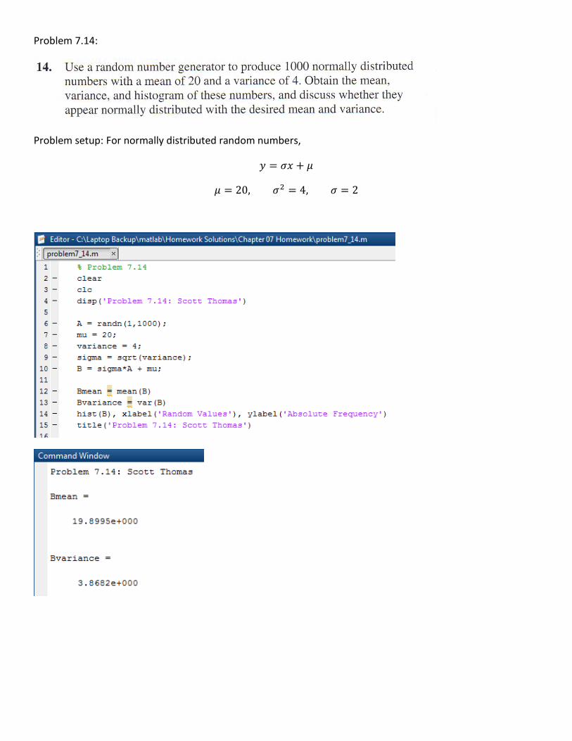
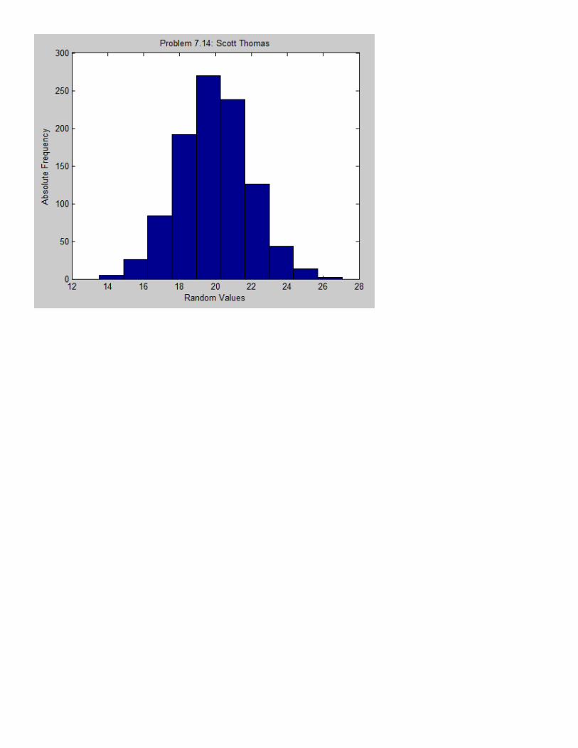
Problem 7.14:

Problem setup: For normally distributed random numbers,

𝑦 = 𝜎𝑥 + 𝜇

𝜇 = 20, 𝜎2 = 4, 𝜎 = 2

Problem 7.16:

Problem 7.23:

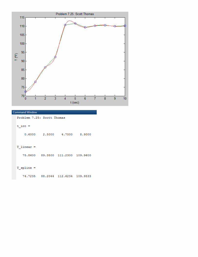
Problem 7.25:

a. Plot the data with open circles, then plot the data by connecting them

first with straight lines and then with a cubic spline.

b. Estimate the temperature values at the following times, using linear

interpolation and then cubic spline interpolation: t = 0.6, 2.5, 4.7, 8.9.