me 1020-02: engineering programming with matlab mid …

Wright State University Fall 2015

Department of Mechanical and Materials Engineering

ME 1020-02: ENGINEERING PROGRAMMING WITH MATLAB

MID-TERM EXAM 3 Open Book, Closed Notes

Create a Separate MATLAB Script File for Each Problem

Submit all MATLAB files (.m) to Dropbox on Pilot

Each MATLAB File Must Have the Following Header:

NAME:

CIRCLE ONE: GRADE MY EXAM DO NOT GRADE MY EXAM

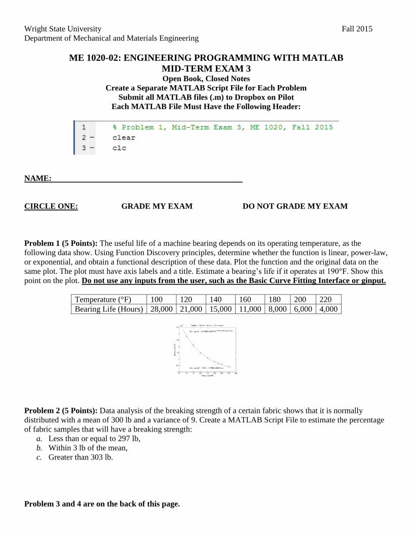
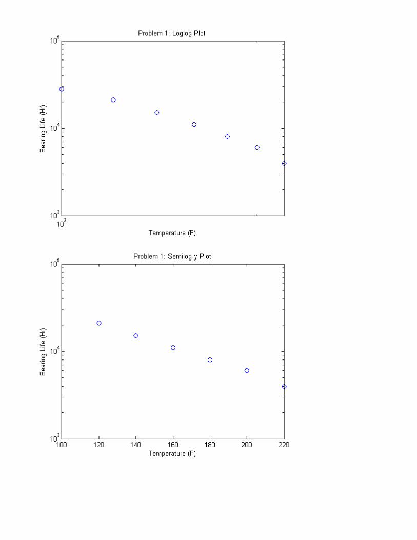
Problem 1 (5 Points): The useful life of a machine bearing depends on its operating temperature, as the

following data show. Using Function Discovery principles, determine whether the function is linear, power-law,

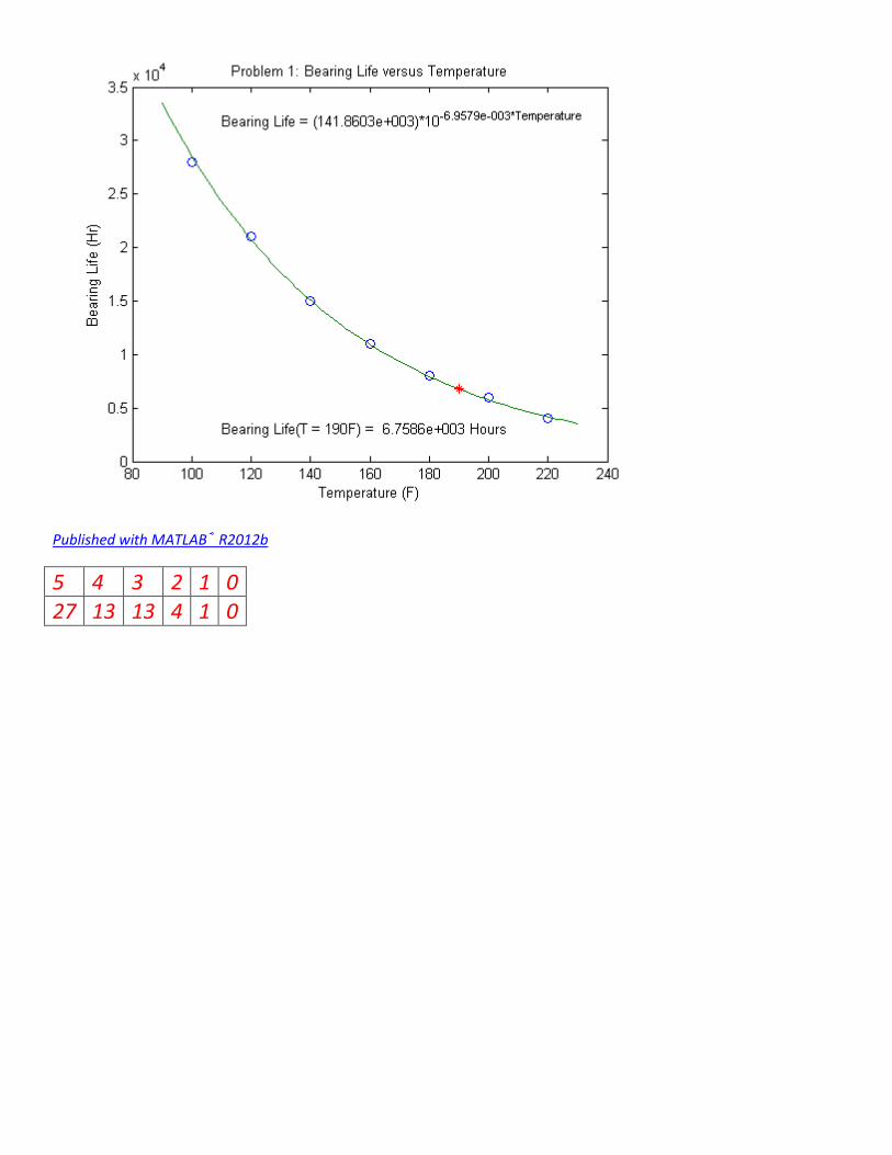
or exponential, and obtain a functional description of these data. Plot the function and the original data on the

same plot. The plot must have axis labels and a title. Estimate a bearing’s life if it operates at 190°F. Show this

point on the plot. Do not use any inputs from the user, such as the Basic Curve Fitting Interface or ginput.

Temperature (°F) 100 120 140 160 180 200 220

Bearing Life (Hours) 28,000 21,000 15,000 11,000 8,000 6,000 4,000

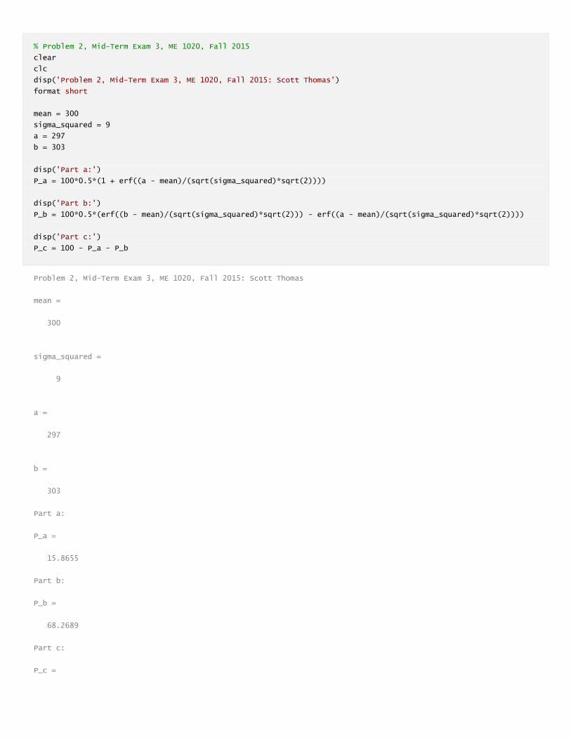
Problem 2 (5 Points): Data analysis of the breaking strength of a certain fabric shows that it is normally

distributed with a mean of 300 lb and a variance of 9. Create a MATLAB Script File to estimate the percentage

of fabric samples that will have a breaking strength:

a. Less than or equal to 297 lb,

b. Within 3 lb of the mean,

c. Greater than 303 lb.

Problem 3 and 4 are on the back of this page.

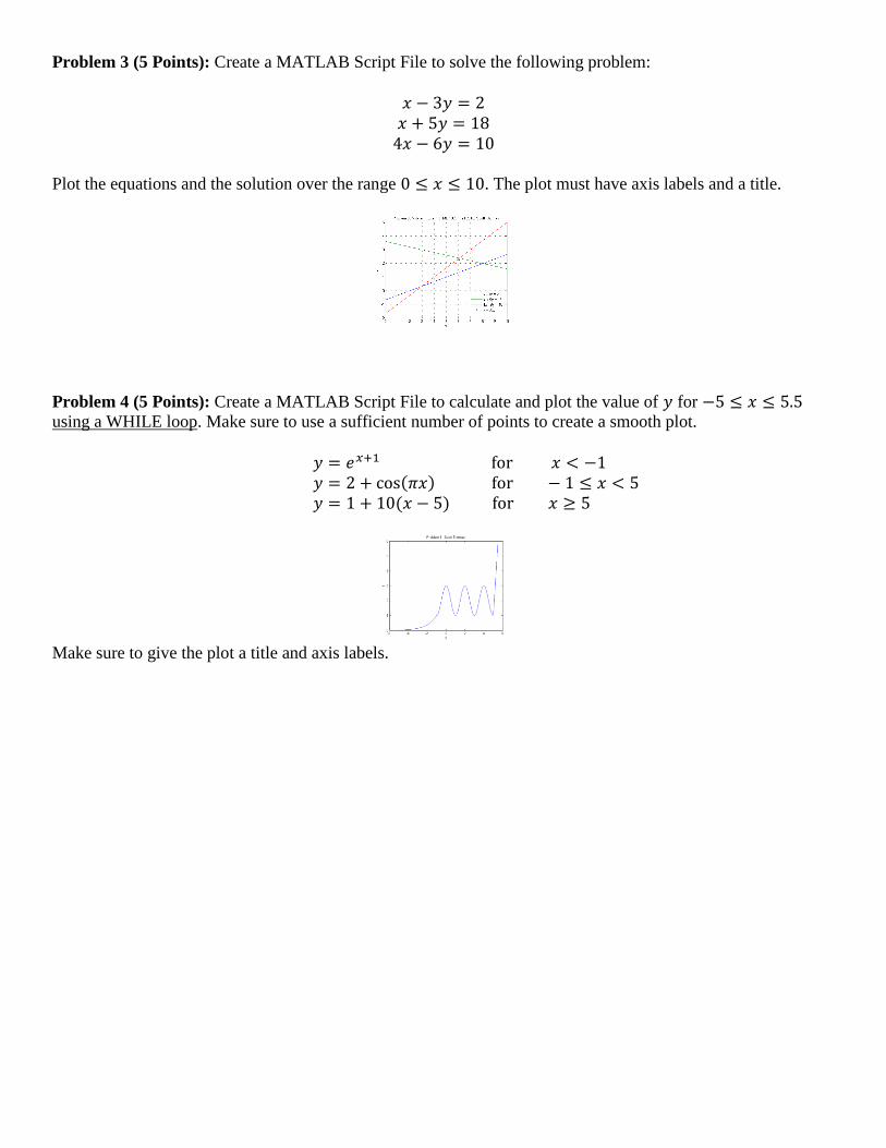
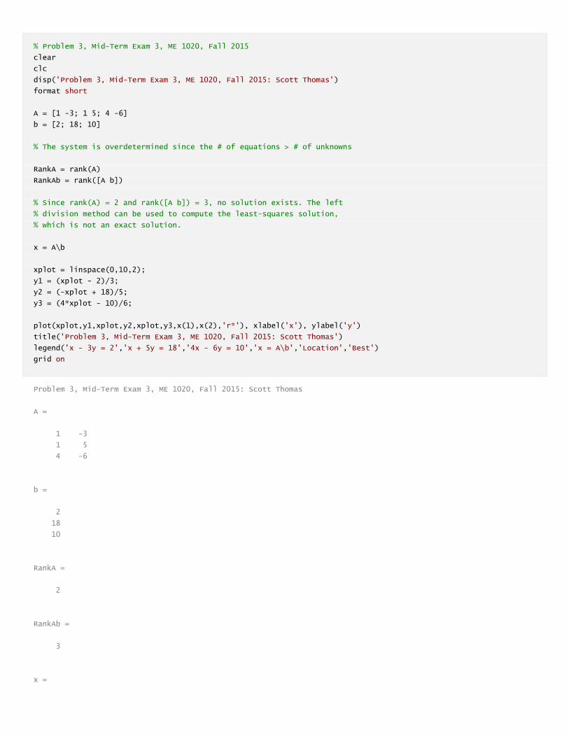
Problem 3 (5 Points): Create a MATLAB Script File to solve the following problem:

𝑥 − 3𝑦 = 2

𝑥 + 5𝑦 = 18

4𝑥 − 6𝑦 = 10

Plot the equations and the solution over the range 0 ≤ 𝑥 ≤ 10. The plot must have axis labels and a title.

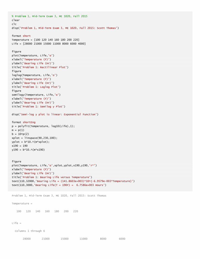
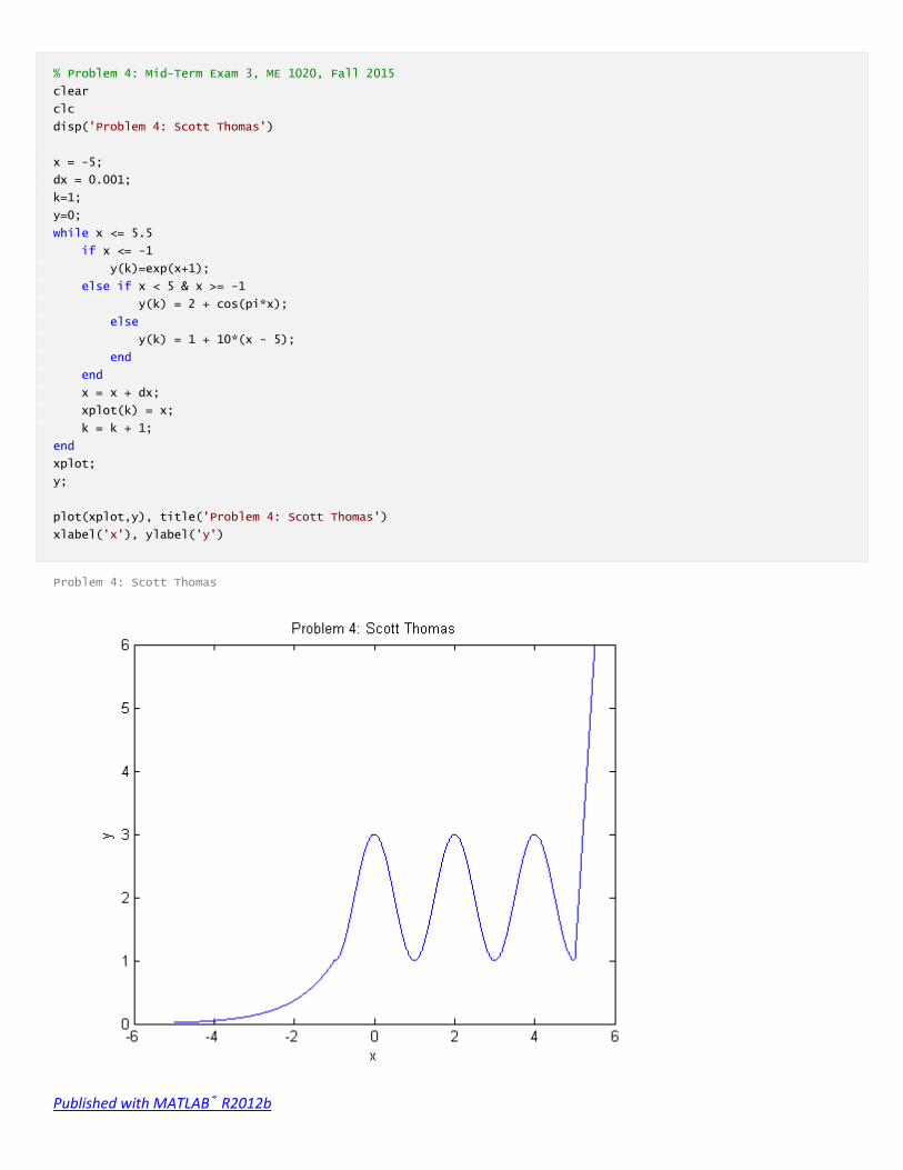
Problem 4 (5 Points): Create a MATLAB Script File to calculate and plot the value of 𝑦 for −5 ≤ 𝑥 ≤ 5.5

using a WHILE loop. Make sure to use a sufficient number of points to create a smooth plot.

𝑦 = 𝑒𝑥+1 for 𝑥 < −1

𝑦 = 2 + cos(𝜋𝑥) for − 1 ≤ 𝑥 < 5

𝑦 = 1 + 10(𝑥 − 5) for 𝑥 ≥ 5

Make sure to give the plot a title and axis labels.

% Problem 1, Mid-Term Exam 3, ME 1020, Fall 2015

clear

clc

disp('Problem 1, Mid-Term Exam 3, ME 1020, Fall 2015: Scott Thomas')

format short

Temperature = [100 120 140 160 180 200 220]

Life = [28000 21000 15000 11000 8000 6000 4000]

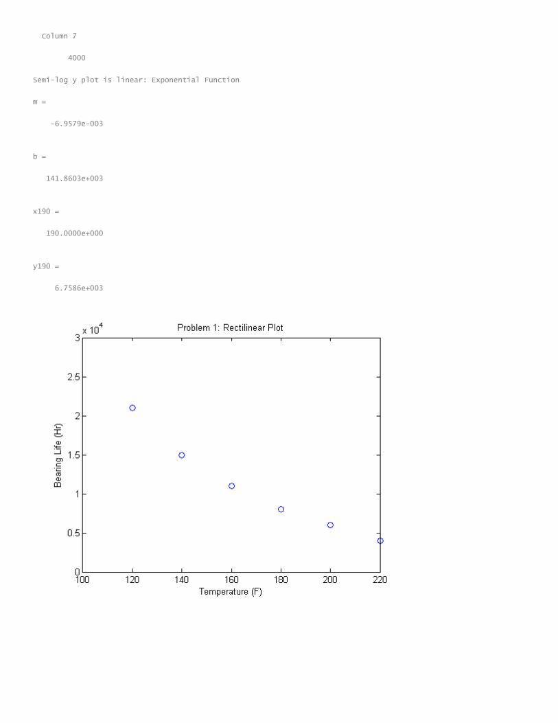
figure

plot(Temperature, Life,'o')

xlabel('Temperature (F)')

ylabel('Bearing Life (Hr)')

title('Problem 1: Rectilinear Plot')

figure

loglog(Temperature, Life,'o')



title('Problem 1: Loglog Plot')

figure

semilogy(Temperature, Life,'o')



title('Problem 1: Semilog y Plot')

disp('Semi-log y plot is linear: Exponential Function')

format shortEng

p = polyfit(Temperature, log10(Life),1);

m = p(1)

b = 10^p(2)

xplot = linspace(90,230,100);

yplot = b*10.^(m*xplot);

x190 = 190

y190 = b*10.^(m*x190)

figure

plot(Temperature, Life,'o',xplot,yplot,x190,y190,'r*')



title('Problem 1: Bearing Life versus Temperature')

text(110,32000,'Bearing Life = (141.8603e+003)*10^{-6.9579e-003*Temperature}')

text(110,3000,'Bearing Life(T = 190F) = 6.7586e+003 Hours')

Problem 1, Mid-Term Exam 3, ME 1020, Fall 2015: Scott Thomas

Temperature =

100 120 140 160 180 200 220

Life =

Columns 1 through 6

28000 21000 15000 11000 8000 6000

Column 7

4000

Semi-log y plot is linear: Exponential Function

m =

-6.9579e-003

b =

141.8603e+003

x190 =

190.0000e+000

y190 =

6.7586e+003

Published with MATLAB® R2012b

5 4 3 2 1 0 27 13 13 4 1 0

http://www.mathworks.com/products/matlab


clear

clc


format short

mean = 300

sigma_squared = 9

a = 297

b = 303

disp('Part a:')

P_a = 100*0.5*(1 + erf((a - mean)/(sqrt(sigma_squared)*sqrt(2))))

disp('Part b:')

P_b = 100*0.5*(erf((b - mean)/(sqrt(sigma_squared)*sqrt(2))) - erf((a - mean)/(sqrt(sigma_squared)*sqrt(2))))

disp('Part c:')

P_c = 100 - P_a - P_b


mean =

300

sigma_squared =

9

a =

297

b =

303

Part a:

P_a =

15.8655

Part b:

P_b =

68.2689

Part c:

P_c =

15.8655


5 4 3 2 1 0 11 10 11 10 12 4



clear

clc


format short

A = [1 -3; 1 5; 4 -6]

b = [2; 18; 10]

% The system is overdetermined since the # of equations > # of unknowns

RankA = rank(A)

RankAb = rank([A b])

% Since rank(A) = 2 and rank([A b]) = 3, no solution exists. The left

% division method can be used to compute the least-squares solution,

% which is not an exact solution.

x = A\b

xplot = linspace(0,10,2);

y1 = (xplot - 2)/3;

y2 = (-xplot + 18)/5;

y3 = (4*xplot - 10)/6;

plot(xplot,y1,xplot,y2,xplot,y3,x(1),x(2),'r*'), xlabel('x'), ylabel('y')

title('Problem 3, Mid-Term Exam 3, ME 1020, Fall 2015: Scott Thomas')

legend('x - 3y = 2','x + 5y = 18','4x - 6y = 10','x = A\b','Location','Best')

grid on


A =

1 -3

1 5

4 -6

b =

2

18

10

RankA =

2

RankAb =

3

x =

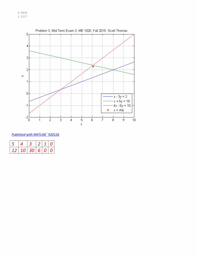
6.0928

2.2577


5 4 3 2 1 0

12 10 30 6 0 0


% Problem 4: Mid-Term Exam 3, ME 1020, Fall 2015

clear

clc

disp('Problem 4: Scott Thomas')

x = -5;

dx = 0.001;

k=1;

y=0;

while x <= 5.5

if x <= -1

y(k)=exp(x+1);

else if x < 5 & x >= -1

y(k) = 2 + cos(pi*x);

else

y(k) = 1 + 10*(x - 5);

end

end

x = x + dx;

xplot(k) = x;

k = k + 1;

end

xplot;

y;

plot(xplot,y), title('Problem 4: Scott Thomas')

xlabel('x'), ylabel('y')

Problem 4: Scott Thomas



5 4 3 2 1 0

8 1 0 14 0 1

me 1020-02: engineering programming with matlab mid …

Documents