MCUAAAR: Methods & Measurement Core Workshop:Structural Equation Models for Longitudinal Analysis of Health Disparities Data

April 11th, 200711:00 to 1:00

ISR 6050

Thomas N. Templin, PhDCenter for Health Research

Wayne State University

Many hypotheses concerning health disparities involve the comparison of longitudinal repeated measures data across one or more groups. A chief advantage of this type of design is that individuals act as their own control reducing confounding.

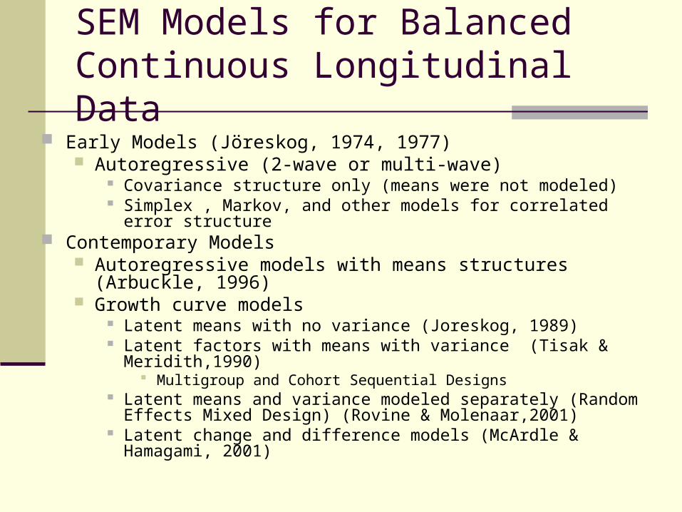
SEM Models for Balanced Continuous Longitudinal Data

Early Models (Jöreskog, 1974, 1977) Autoregressive (2-wave or multi-wave)

Covariance structure only (means were not modeled) Simplex , Markov, and other models for correlated error structure

Contemporary Models Autoregressive models with means structures (Arbuckle, 1996) Growth curve models

Latent means with no variance (Joreskog, 1989) Latent factors with means with variance (Tisak & Meridith,1990)

Multigroup and Cohort Sequential Designs Latent means and variance modeled separately (Random Effects

Mixed Design) (Rovine & Molenaar,2001) Latent change and difference models (McArdle & Hamagami, 2001)

SEM Models for Balanced Continuous Longitudinal Data

Contemporary Models (cont.) Growth curve models (cont)

Growth models for experimental designs (Muthen &Curran, 1997) Biometric Models (McArdle, et al,1998) Pooled interrupted time series model (Duncan & Duncan, 2004)

Latent class GC models (Muthen, M-Plus) Multilevel GC models

MG-Latent Identity Basis Model

Unlike the familiar two-wave autoregressive model, latent growth curve and change and difference models involve a different approach to SEM modeling.

Many of these models appear to be variations of one another.

I formulated what I am calling a multigroup latent identitly basis model (MG-LBM) that serves as a starting point for more specific longitudinal models.

I will formulate this for model and then derive latent difference and growth, random effects, and other kinds of models that have appeared in the literature

MG-Latent Basis Model

Two Parts Means Structure

Within group coding of within subject contrasts. Test parameters by comparing models with and without

equality constraints Between plus within-group coding.

Test parameters directly.

Covariance Structure Model error directly (replace error covariances with

latent factors, etc) Model error indirectly (add latent structure to

prediction equations)

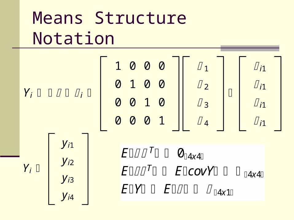
Means Structure Notation

Yi i

1 0 0 0

0 1 0 0

0 0 1 0

0 0 0 1

1

2

3

4

i1 i1 i1 i1

Yi

y i1

y i2

y i3

y i4

E T 04x4

E T EcovY 4x4

EY E 4x1

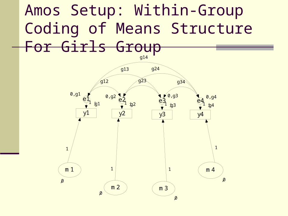
Amos Setup: Within-Group Coding of Means Structure For Girls Group

ig1

y1

0, g1e1

1 ig2

y2

0, g2e2

1 ig3

y3

0, g3e3

1 ig4

y4

0, g4e4

1

g34

g14

g12

g24

g23

g13

,0m2

,0

m3

1 1

,0

m1

1

,0

m4

1

Amos Setup : Within-Group Coding For Boys Group

ib1

y1

0, b1e1

1 ib2

y2

0, b2e2

1 ib3

y3

0, b3e3

1 ib4

y4

0, b4e4

1

b34

b14

b12

b24

b23

b13

,0m2

,0

m3

1 1

,0

m1

1

,0

m4

1

Within-Group Coding

Parameter constraints identified in “manage models”All intercepts are constrained to 0.

ib1 = ib2 = ib3 = ib4 = ig1 = ig2 = ig3 = ig4=0

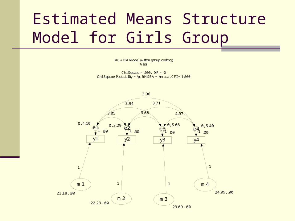
Estimated Means Structure Model for Girls Group

MG-LBM Model (within group coding)Girls

Chi Square = .000, DF = 0Chi Square Probability = \p, RMSEA = \rmsea, CFI = 1.000

.00

y1

0, 4.10e1

1 .00

y2

0, 3.29e2

1 .00

y3

0, 5.08e3

1 .00

y4

0, 5.40e4

1

4.97

3.96

3.05

3.71

3.66

3.94

22.23, .00m2

23.09, .00

m3

1 1

21.18, .00

m1

1

24.09, .00

m4

1

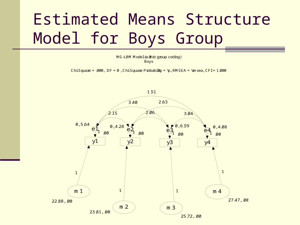
Estimated Means Structure Model for Boys Group

MG-LBM Model (within group coding)Boys

Chi Square = .000, DF = 0 , Chi Square Probability = \p, RMSEA = \rmsea, CFI = 1.000

.00

y1

0, 5.64e1

1 .00

y2

0, 4.28e2

1 .00

y3

0, 6.59e3

1 .00

y4

0, 4.08e4

1

3.04

1.51

2.15

2.63

2.06

3.40

23.81, .00m2

25.72, .00

m3

1 1

22.88, .00

m1

1

27.47, .00

m4

1

Contrast Coding Across Groups

In order to explicitly estimate between group effects and interactions you need one design matrix for within and between effects.

The more general coding described next will provide a foundation for this.

With 4 repeated measures and 2 groups a total of 8 contrasts or identity vectors are needed.

The same 8 means will be estimated but now there is one design matrix across both groups.

This is achieved by constraining parameter estimates for each of the 8 identity vectors to be equal across groups

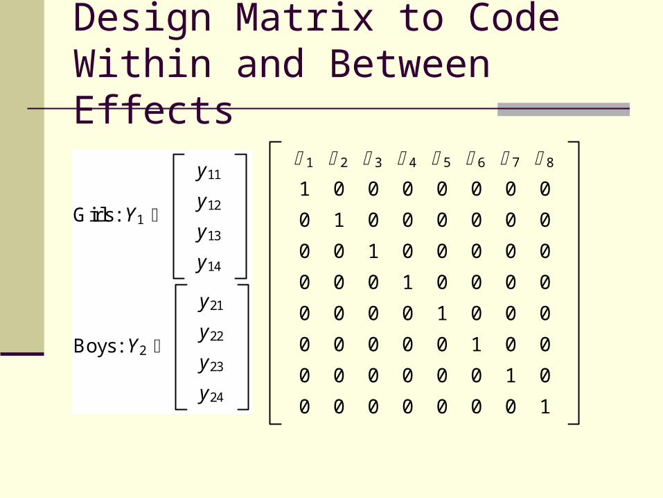
Design Matrix to Code Within and Between Effects

Girls: Y1

y11

y12

y13

y14

Boys: Y2

y21

y22

y23

y24

1 2 3 4 5 6 7 8

1 0 0 0 0 0 0 0

0 1 0 0 0 0 0 0

0 0 1 0 0 0 0 0

0 0 0 1 0 0 0 0

0 0 0 0 1 0 0 0

0 0 0 0 0 1 0 0

0 0 0 0 0 0 1 0

0 0 0 0 0 0 0 1

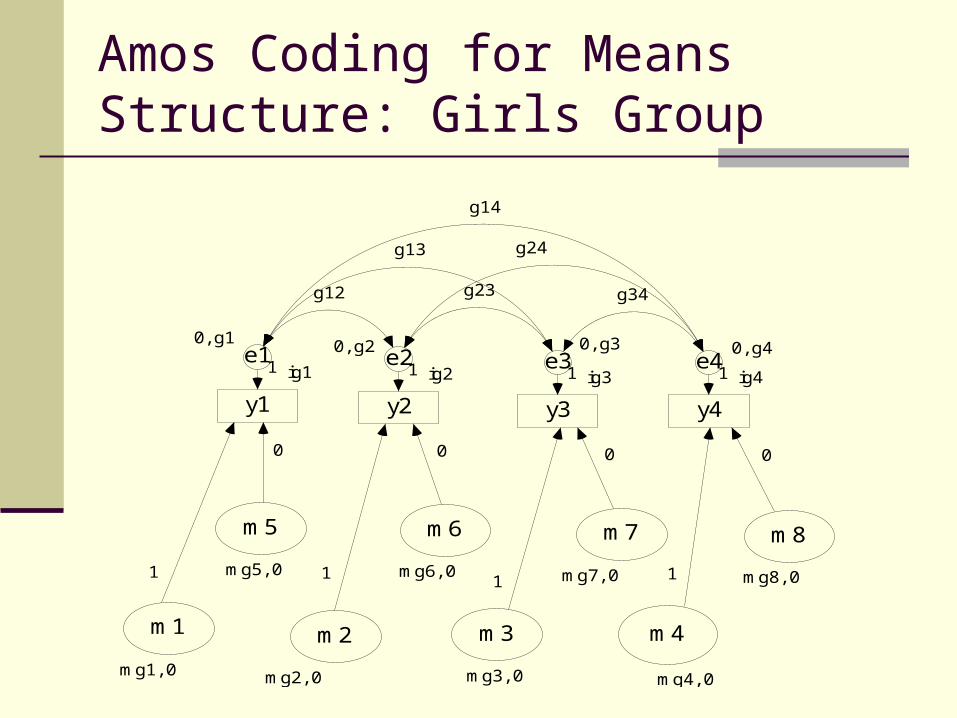
Amos Coding for Means Structure: Girls Group

ig1

y1

0, g1e1

1 ig2

y2

0, g2e2

1 ig3

y3

0, g3e3

1 ig4

y4

0, g4e4

1

g34

g14

g12

g24

g23

g13

mg2, 0

m2

mg3, 0

m3

1 1

mg1, 0

m1

1

mg4, 0

m4

mg5, 0

m5

mg6, 0

m6

mg7, 0

m7

mg8, 0

m8

1

0 0 0 0

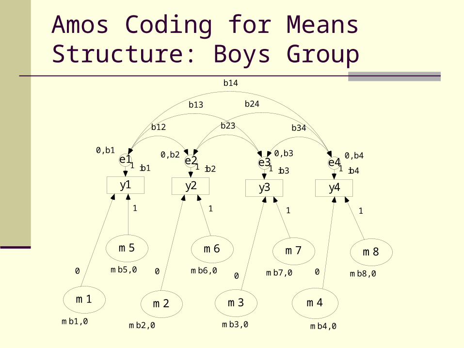
Amos Coding for Means Structure: Boys Group

ib1

y1

0, b1e1

1 ib2

y2

0, b2e2

1 ib3

y3

0, b3e3

1 ib4

y4

0, b4e4

1

b34

b14

b12

b24

b23

b13

mb2, 0

m2

mb3, 0

m3

0 0

mb1, 0

m1

0

mb4, 0

m4

mb5, 0

m5

mb6, 0

m6

mb7, 0

m7

mb8, 0

m8

0

1 1 1 1

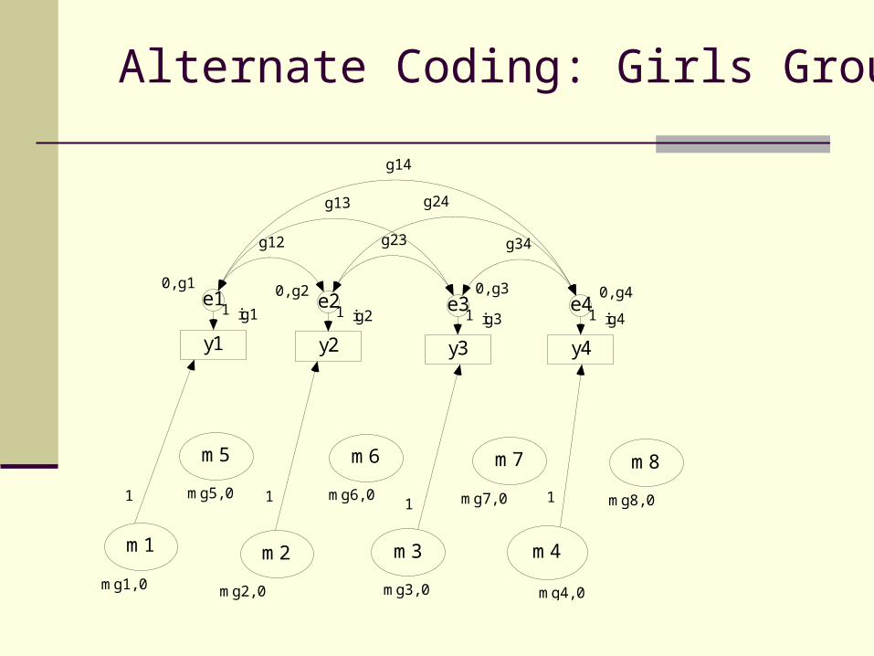
Alternate Coding: Girls Group

ig1

y1

0, g1e1

1 ig2

y2

0, g2e2

1 ig3

y3

0, g3e3

1 ig4

y4

0, g4e4

1

g34

g14

g12

g24

g23

g13

mg2, 0

m2

mg3, 0

m3

1 1

mg1, 0

m1

1

mg4, 0

m4

mg5, 0

m5

mg6, 0

m6

mg7, 0

m7

mg8, 0

m8

1

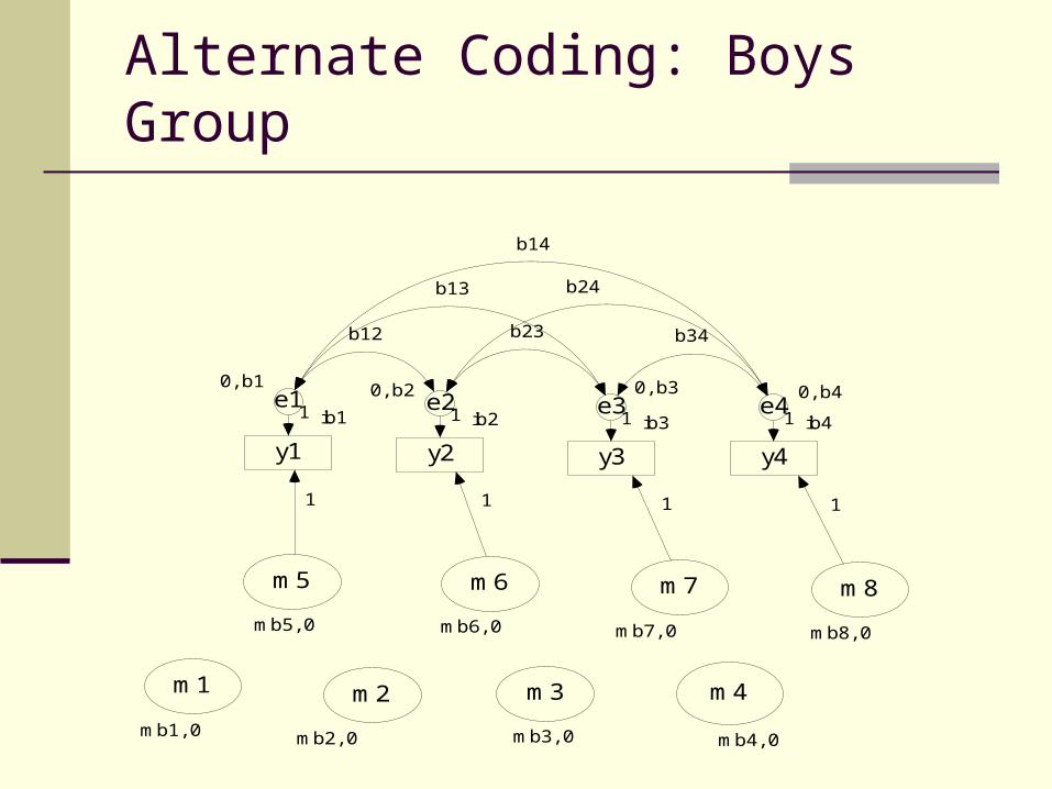
Alternate Coding: Boys Group

ib1

y1

0, b1e1

1 ib2

y2

0, b2e2

1 ib3

y3

0, b3e3

1 ib4

y4

0, b4e4

1

b34

b14

b12

b24

b23

b13

mb2, 0

m2

mb3, 0

m3

mb1, 0

m1

mb4, 0

m4

mb5, 0

m5

mb6, 0

m6

mb7, 0

m7

mb8, 0

m8

1 1 1 1

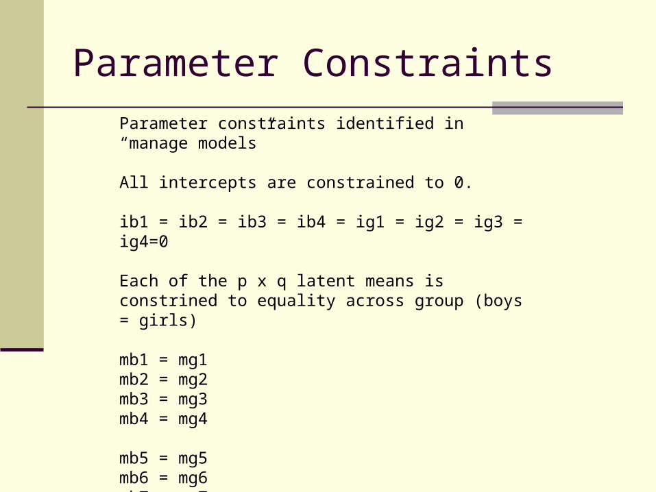
Parameter ConstraintsParameter constraints identified in “manage models”

All intercepts are constrained to 0.

ib1 = ib2 = ib3 = ib4 = ig1 = ig2 = ig3 = ig4=0

Each of the p x q latent means is constrined to equality across group (boys = girls)

mb1 = mg1mb2 = mg2mb3 = mg3mb4 = mg4

mb5 = mg5 mb6 = mg6mb7 = mg7mb8 = mg8

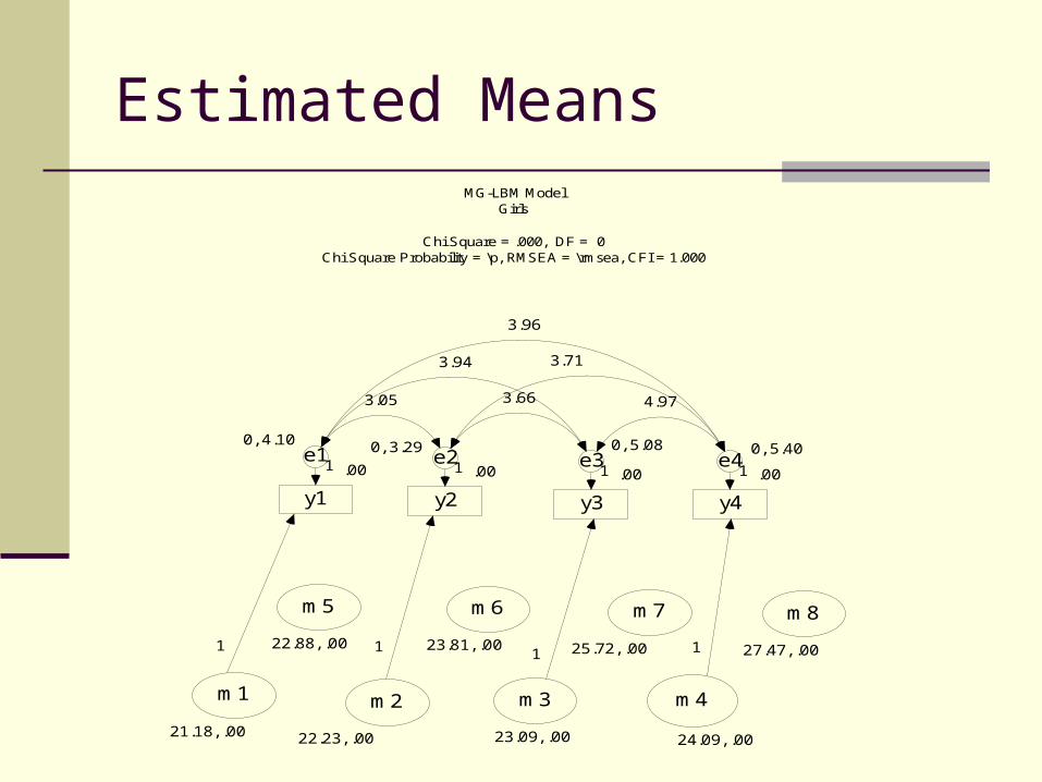
Estimated MeansMG-LBM Model

Girls

Chi Square = .000, DF = 0Chi Square Probability = \p, RMSEA = \rmsea, CFI = 1.000

.00

y1

0, 4.10e1

1 .00

y2

0, 3.29e2

1 .00

y3

0, 5.08e3

1 .00

y4

0, 5.40e4

1

4.97

3.96

3.05

3.71

3.66

3.94

22.23, .00

m2

23.09, .00

m3

1 1

21.18, .00

m1

1

24.09, .00

m4

22.88, .00

m5

23.81, .00

m6

25.72, .00

m7

27.47, .00

m8

1

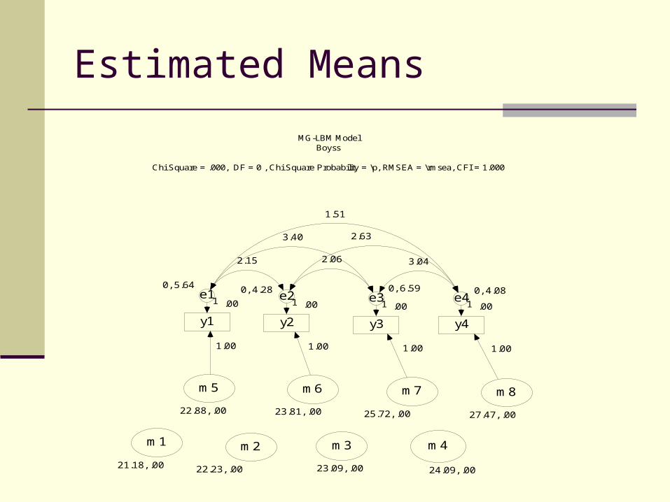
Estimated Means

MG-LBM ModelBoyss

Chi Square = .000, DF = 0 , Chi Square Probability = \p, RMSEA = \rmsea, CFI = 1.000

.00

y1

0, 5.64e1

1 .00

y2

0, 4.28e2

1 .00

y3

0, 6.59e3

1 .00

y4

0, 4.08e4

1

3.04

1.51

2.15

2.63

2.06

3.40

22.23, .00

m2

23.09, .00

m3

21.18, .00

m1

24.09, .00

m4

22.88, .00

m5

23.81, .00

m6

25.72, .00

m7

27.47, .00

m8

1.00 1.00 1.00 1.00

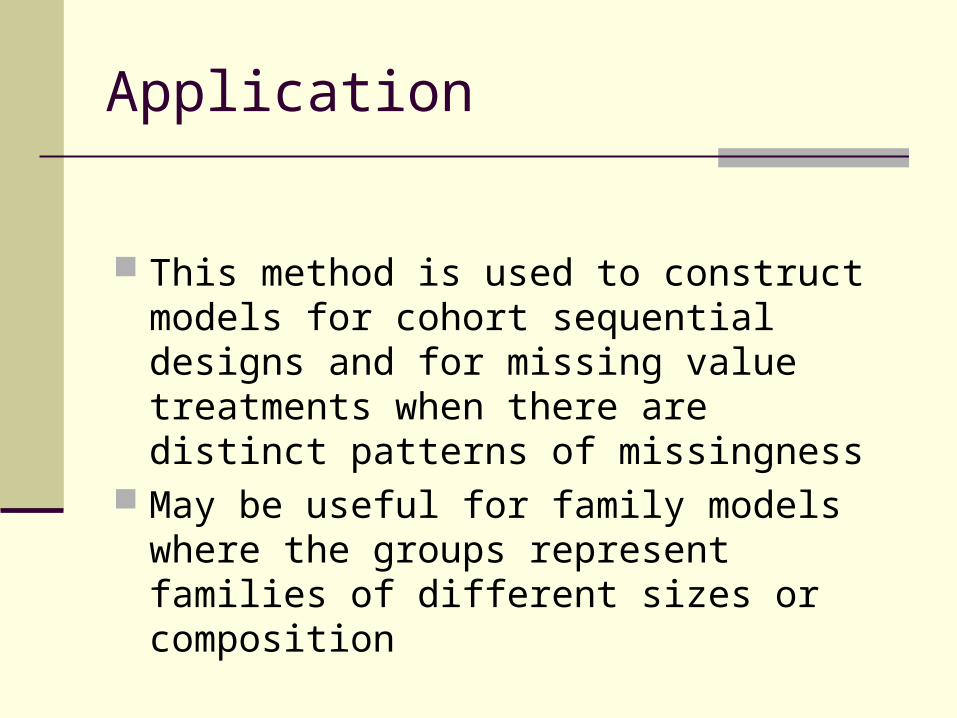
Application

This method is used to construct models for cohort sequential designs and for missing value treatments when there are distinct patterns of missingness

May be useful for family models where the groups represent families of different sizes or composition

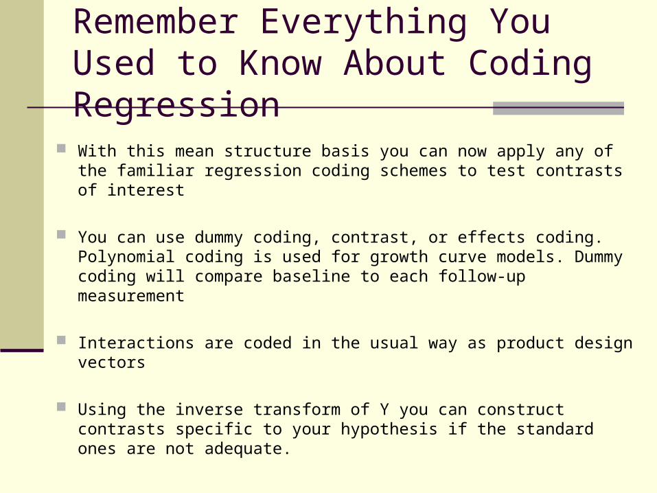
Remember Everything You Used to Know About Coding Regression

With this mean structure basis you can now apply any of the familiar regression coding schemes to test contrasts of interest

You can use dummy coding, contrast, or effects coding. Polynomial coding is used for growth curve models. Dummy coding will compare baseline to each follow-up measurement

Interactions are coded in the usual way as product design vectors

Using the inverse transform of Y you can construct contrasts specific to your hypothesis if the standard ones are not adequate.

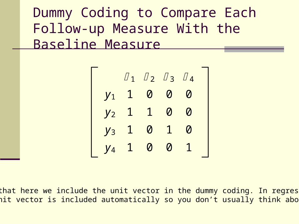
Dummy Coding to Compare Each Follow-up Measure With the Baseline Measure

1 2 3 4

y1 1 0 0 0

y2 1 1 0 0

y3 1 0 1 0

y4 1 0 0 1

Note that here we include the unit vector in the dummy coding. In regression,the unit vector is included automatically so you don’t usually think about it.

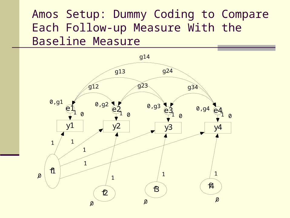
Amos Setup: Dummy Coding to Compare Each Follow-up Measure With the Baseline Measure

0

y1

0, g1e1

1 0

y2

0, g2e2

1 0

y3

0, g3e3

1 0

y4

0, g4 e41

g34

g14

g12

g24

g23

g13

,0f1

,0

f2,0

f3,0

f4

1

1

11

11 1

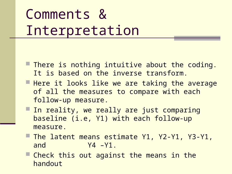
Comments & Interpretation

There is nothing intuitive about the coding. It is based on the inverse transform.

Here it looks like we are taking the average of all the measures to compare with each follow-up measure.

In reality, we really are just comparing baseline (i.e, Y1) with each follow-up measure.

The latent means estimate Y1, Y2-Y1, Y3-Y1, and Y4 –Y1.

Check this out against the means in the handout

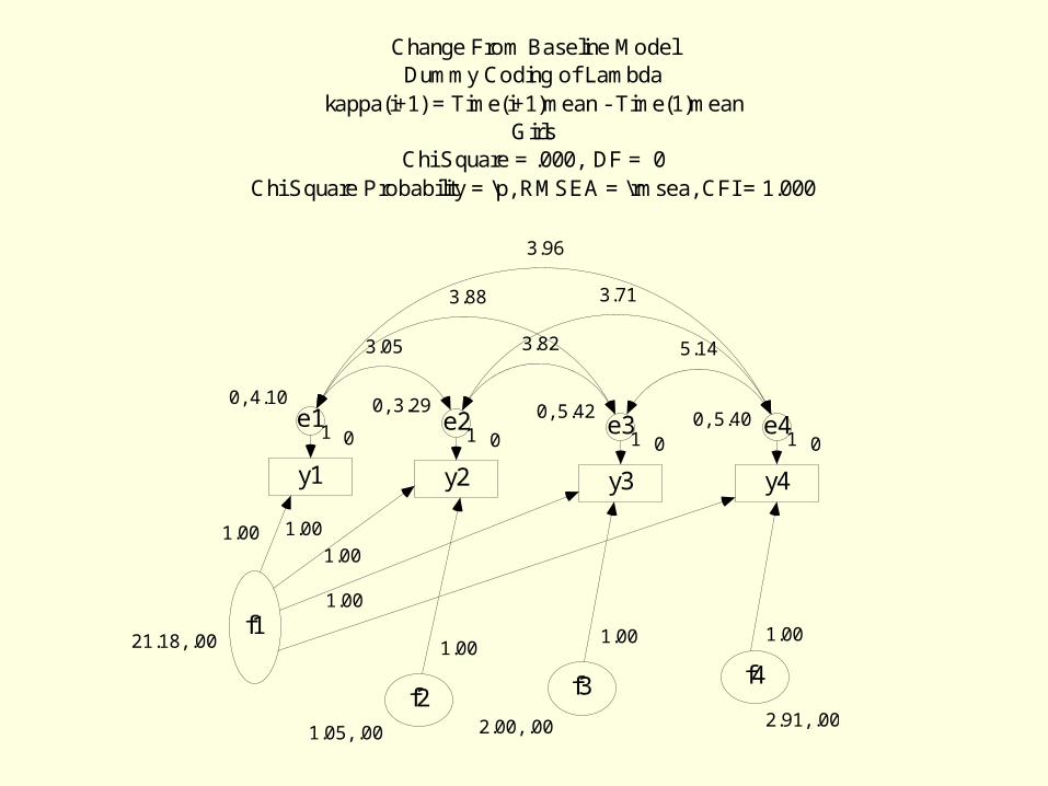
Change From Baseline ModelDummy Coding of Lambda

kappa(i+1) = Time(i+1)mean - Time(1)meanGirls

Chi Square = .000, DF = 0Chi Square Probability = \p, RMSEA = \rmsea, CFI = 1.000

0

y1

0, 4.10e1

1 0

y2

0, 3.29e2

1 0

y3

0, 5.42e3

1 0

y4

0, 5.40 e41

5.14

3.96

3.05

3.71

3.82

3.88

21.18, .00f1

1.05, .00

f22.00, .00

f32.91, .00

f4

1.00

1.00

1.001.00

1.001.00 1.00

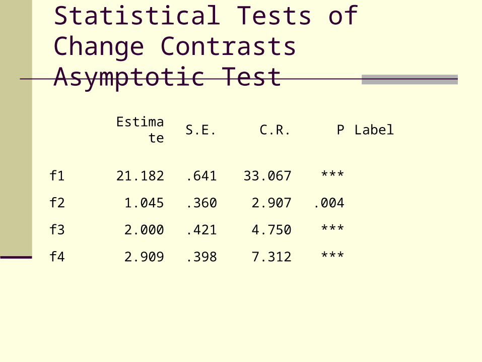
Statistical Tests of Change ContrastsAsymptotic Test

Estimate S.E. C.R. P Label

f1 21.182 .641 33.067 ***

f2 1.045 .360 2.907 .004

f3 2.000 .421 4.750 ***

f4 2.909 .398 7.312 ***

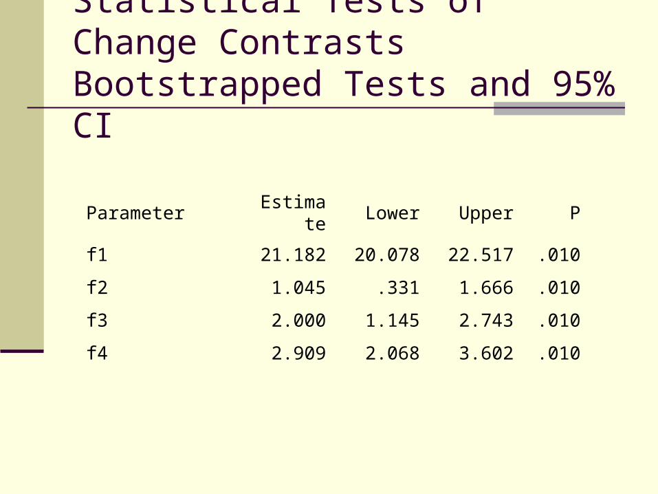
Statistical Tests of Change ContrastsBootstrapped Tests and 95% CI

Parameter Estimate Lower Upper P

f1 21.182 20.078 22.517 .010

f2 1.045 .331 1.666 .010

f3 2.000 1.145 2.743 .010

f4 2.909 2.068 3.602 .010

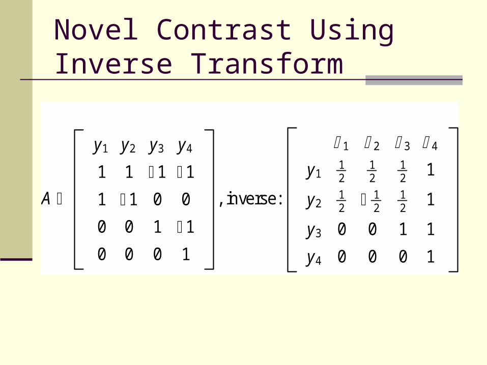
Novel Contrast Using Inverse Transform

A

y1 y2 y3 y4

1 1 1 1

1 1 0 0

0 0 1 1

0 0 0 1

, inverse:

1 2 3 4

y112

12

12

1

y212

12

12

1

y3 0 0 1 1

y4 0 0 0 1

Novel Coding Using Inverse TransformGirls

Chi Square = .000, DF = 0, Chi Square Probability = \p,RMSEA = \rmsea, CFI = 1.000

0

y1

0, 4.10e1

1 0

y2

0, 3.29e2

1 0

y3

0, 5.42e3

1 0

y4

0, 5.40 e41

5.14

3.96

3.05

3.71

3.82

3.88

-3.86, .00f1

-1.05, .00 f2-.91, .00

f324.09, .00

f4

1.00.50

1.00

1.001.00

.50

.50 -.50

.50.50

1.00

Growth Curve Model with Fixed Effects OnlyJöreskog, 1989

m1

y1

0, g1

e11 m2

y2

0, g2

e21 m3

y3

0, g3

e31 m4

y4

0, g4

e41

g34

g14

g12

g24

g23

g13

,0ICEPT

,0Slope

1 1

1 0

12

4

6

Girls

m1

y1

0, b1

e11 m2

y2

0, b2

e21 m3

y3

0, b3

e31 m4

y4

0, b4

e41

b34

b14

b12

b24

b23

b13

,0ICEPT

,0Slope

1 1

1 0

12

4

6

Boys

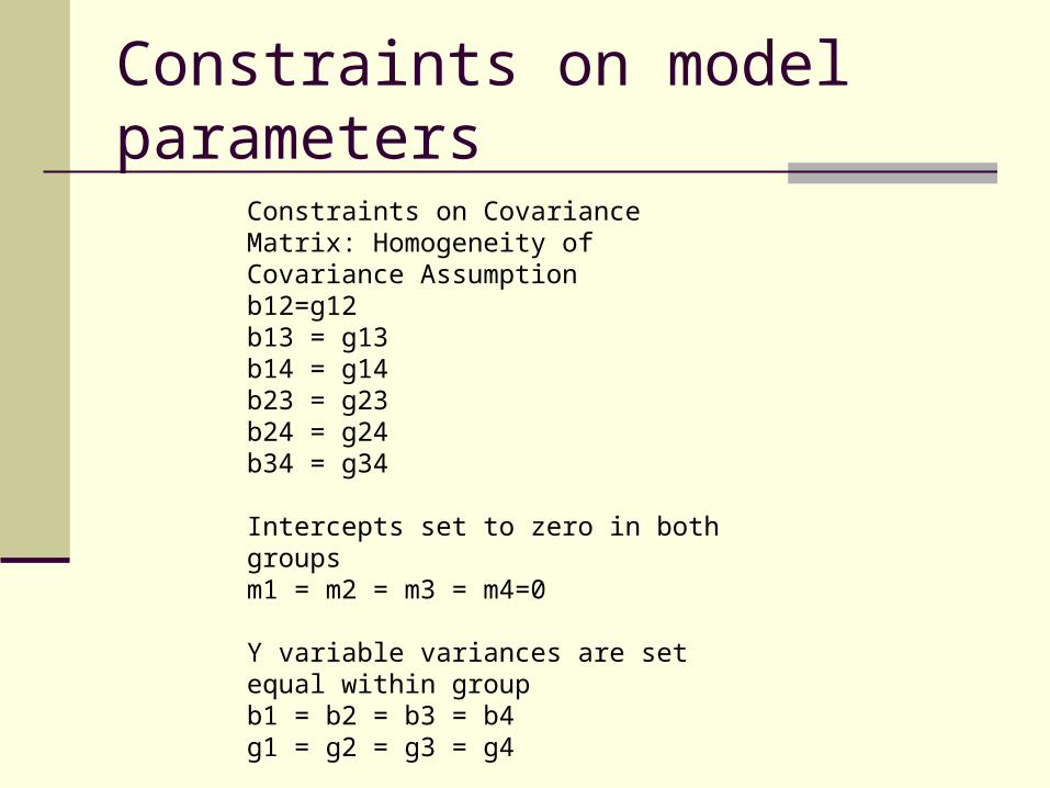
Constraints on model parameters

Constraints on Covariance Matrix: Homogeneity of Covariance Assumptionb12=g12b13 = g13b14 = g14b23 = g23b24 = g24b34 = g34

Intercepts set to zero in both groupsm1 = m2 = m3 = m4=0

Y variable variances are set equal within groupb1 = b2 = b3 = b4g1 = g2 = g3 = g4

Growth Curve ModelGirls

Joreskog & Sorbom (1989, LISREL 7 User Guide, 2nd Ed., p 261)

Chi Square = 11.454, DF = 16Chi Square Probability = .781, RMSEA = .000, CFI = 1.000

.00

y1

0, 3.70

e11 .00

y2

0, 3.70

e21 .00

y3

0, 3.70

e31 .00

y4

0, 3.70

e41

3.45

2.94

2.97

3.08

3.15

2.90

21.23, .00ICEPT

.48, .00Slope

1.00 1.00

1.00 .00

1.002.00

4.00

6.00

Growth Curve ModelBoys

(Pottoff & Roy, 1964)Joreskog & Sorbom (1989, LISREL 7 User Guide, 2nd Ed., p 261)

Chi Square = 11.454, DF = 16 , Chi Square Probability = .781, RMSEA = .000, CFI = 1.000

.00

y1

0, 5.84

e11 .00

y2

0, 5.84

e21 .00

y3

0, 5.84

e31 .00

y4

0, 5.84

e41

3.45

2.94

2.97

3.08

3.15

2.90

22.60, .00ICEPT

.79, .00Slope

1.00 1.00

1.00 .00

1.002.00

4.00

6.00

Compare toData in Handout

Do the slope and intercept estimates look Reasonable for each group?

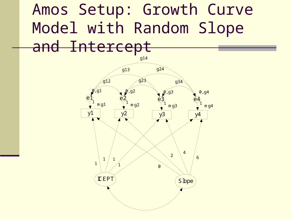
Part II: Covariance Structure for Correlated Observations

Standard techniques like we OLS regression, ANOVA, and MANOVA compare means and leave the correlated error unanalyzed.

The SEM approach, and modern regression procedures like HLM, tap the information in the correlation structure.

Latent structure can be brought out of the error side or the observed variable side of the model.

mg1

y1

0, g1

e11

mg2

y2

0, g2

e21

mg3

y3

0, g3

e31

mg4

y4

0, g4

e41

g34

g14

g12

g24

g23

g13

ICEPT Slope

10

12

1

4

1

6

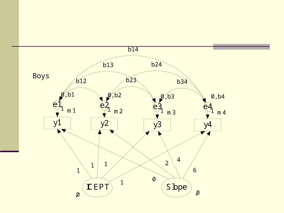
Amos Setup: Growth Curve Model with Random Slope and Intercept

Model Constraints

Correlations among error terms are fixed to 0

b12=g12=0b13 = g13=0b14 = g14=0b23 = g23=0b24 = g24=0b34 = g34=0

b3 = b4

Intercepts fixed to 0.

m1 = m2 = m3 = m4 = mg1 = mg2 = mg3 = mg4=0

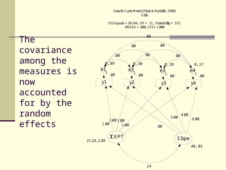
The covariance among the measures is now accounted for by the random effects

Growth Curve Model (Tisak & Meridith, 1990)Girls

Chi Square = 10.144, DF = 11, Probability = .517,RMSEA = .000, CFI = 1.000

.00

y1

0, .89

e11

.00

y2

0, .50

e21

.00

y3

0, .39

e31

.00

y4

0, .17

e41

.00

.00

.00

.00

.00

.00

21.24, 2.88ICEPT

.48, .02

Slope

.14

1.00.00

1.002.00

1.00

4.00

1.00

6.00

Growth Curve ModelBoys

Chi Square = 10.144, DF = 11 Probability = .517RMSEA = .000, CFI = 1.000

.00

y1

0, 3.78

e11

.00

y2

0, 2.36

e21

.00

y3

0, 2.55

e31

.00

y4

0, 2.55

e41

.00

.00

.00

.00

.00

.00

22.51, 2.11ICEPT

.81, -.01

Slope

.06

1.00.00

1.002.00

1.00

4.00

1.00

6.00

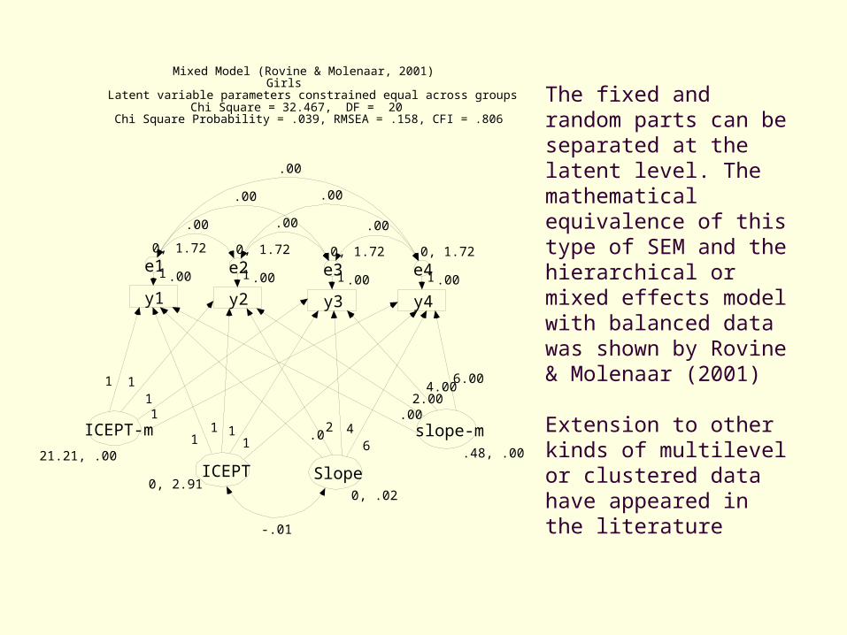
The fixed and random parts can be separated at the latent level. The mathematical equivalence of this type of SEM and the hierarchical or mixed effects model with balanced data was shown by Rovine & Molenaar (2001)

Extension to other kinds of multilevel or clustered data have appeared in the literature

Mixed Model (Rovine & Molenaar, 2001)Girls

Latent variable parameters constrained equal across groupsChi Square = 32.467, DF = 20

Chi Square Probability = .039, RMSEA = .158, CFI = .806

.00

y1

0, 1.72

e11 .00

y2

0, 1.72

e21 .00

y3

0, 1.72

e31 .00

y4

0, 1.72

e41

.00

.00

.00

.00

.00

.00

0, 2.91ICEPT

0, .02

Slope

1 11

.012 4

6

-.01

21.21, .00

ICEPT-m

1 111

.48, .00

slope-m

6.004.00

2.00.00

m1

y1

0, b1

e11 m2

y2

0, b2

e21

m3

y3

0, b3

e31

m4

y4

0, b4

e41

b34

b14

b12

b24

b23

b13

ICEPT Slope0

1 214

1 6

0

HealthOutcome

0,

1

10,

10,

1

1

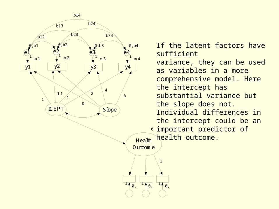
If the latent factors have sufficientvariance, they can be used as variables in a more comprehensive model. Here the intercept has substantial variance but the slope does not. Individual differences in the intercept could be an important predictor of health outcome.

Here individual differences in the intercept are modeled as a mediator of health outcome

m1

y1

0, b1

e11 m2

y2

0, b2

e21

m3

y3

0, b3

e31

m4

y4

0, b4

e41

b34

b14

b12

b24

b23

b13

ICEPT Slope0

1 21

4

16

0

HealthOutcome

0,

1

10,

10,

1

1Variable Correlated With Race/Ethnicity

0,1

Time

Y

0

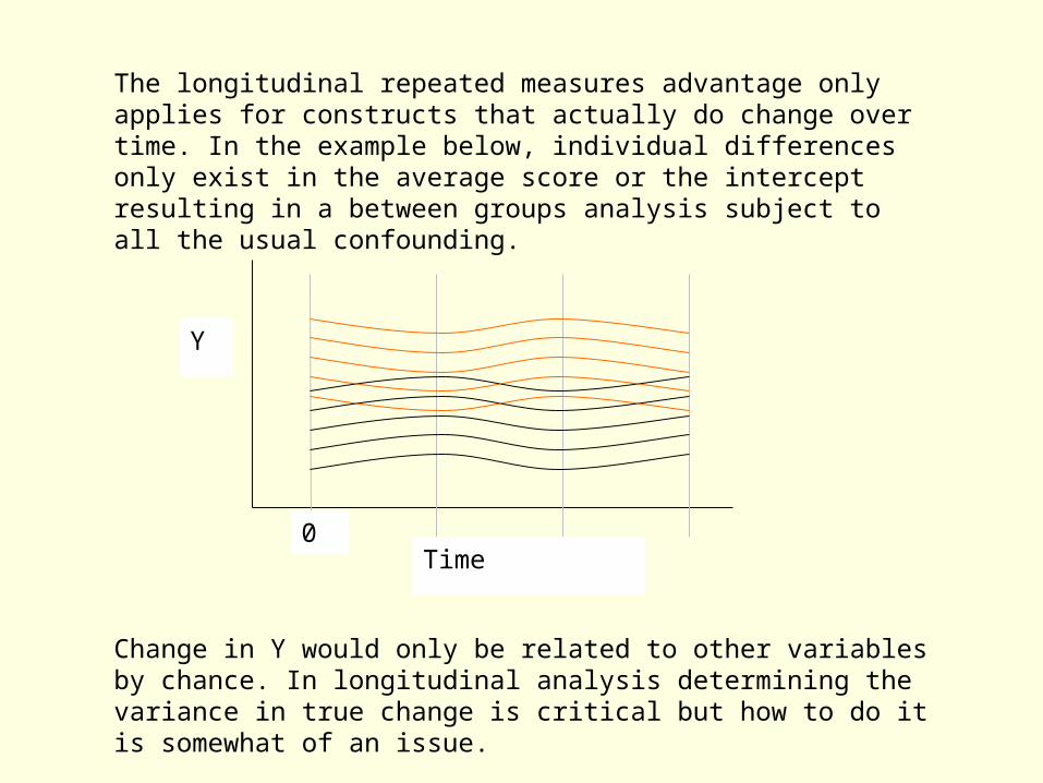
The longitudinal repeated measures advantage only applies for constructs that actually do change over time. In the example below, individual differences only exist in the average score or the intercept resulting in a between groups analysis subject to all the usual confounding.

Change in Y would only be related to other variables by chance. In longitudinal analysis determining the variance in true change is critical but how to do it is somewhat of an issue.

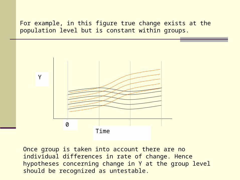
For example, in this figure true change exists at the population level but is constant within groups.

Time

Y

0

Once group is taken into account there are no individual differences in rate of change. Hence hypotheses concerning change in Y at the group level should be recognized as untestable.

Pooled Interrupted Time Series AnalysesDuncan & Duncan, 2004

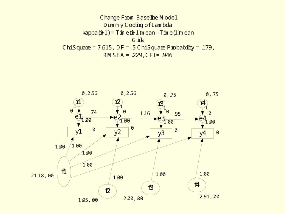
Change From Baseline ModelDummy Coding of Lambda

kappa(i+1) = Time(i+1)mean - Time(1)meanGirls

Chi Square = 7.615, DF = 5 Chi Square Probability = .179,RMSEA = .229, CFI = .946

0y1

0e1

1.00

0y2

0e2

1.00

0y3

0

e31.00

0y4

0e4

1.00

21.18, .00f1

1.05, .00

f22.00, .00

f32.91, .00

f4

1.00

1.00

1.001.00

1.001.00 1.00

.74 1.16 .95

0, 2.56

r21

0, .75

r31

0, .75

r41

0, 2.56

r11

ICEPT SLOPE

X1 X2 X3 X4

E1

1

E2

1

E3

1

E4

1

Amos defaultGrowth model