longitudinal forced vibration of viscoelastic … · computer generated curves and discussion 7 ......

SR 135

COREL Special Rsport 135

O LONGITUDINAL FORCED VIBRATION

OF VISCOELASTIC BARS WITH END MASS

D.M. Morris,Jr. and

Wun-Chung Young

April 1970

C L A « I N G H Ü U '. i fc.r i".' ).•>„ ■ ' ■ ■,!... . In: - ■• n i,' ■• ,' ■ I ■ , 1

D n n

GRANT NO. DA-AMC-27-021-67-G:

CORPS OF ENGINEERS, U.S. ARMY

COLD REGIONS RESEARCH AND ENGINEERING LABORATORY HANOVER, NEW HAMPSHIRE

THIS DOCUMENT HAS BEEN APPROVED FOR PUBLIC RELEASE AND SALE, ITS DISTRIBUTION IS UNLIMITED.

}>

LONGITUDINAL FORCED VIBRATION OF VISCOELASTIC BARS

WITH END MASS

D.M. Norrisjr. and

Wun-Chung Young

April 1970

GRANT NO. DA-AMC-27-021-67-G21

DA TASK 1T062t12A13001

CORPS OF ENGINEERS, U.S. ARMY

COLD REGIONS RESEARCH AND ENGINEERING LABORATORY HANOVER, NEW HAMPSHIRE

THIS DOCUMENT HAS BEEN APPROVED POR PUBLIC REi EASE AND SALE; ITS DISTRIBUTION IS UNLIMITED.

ii

PREFACE

This report was prepared by Dr. D.M. Norris, Jr., Associate Professor of Mechanics, of the University of New Hampshire, and Mr. Wun-Chung Young, presently Project Engineer, Combustion Engineering, Inc., Windsor, Connecticut. The work was performed for the U.S. Army Cold Regions Research and Engineering Laboratory (USA CRREL), under Grant No. DA-AMC-27-021-67-O21.

The work was under the supervision of Mr. A.F. Wuori, Chief, Applied Research Branch, and under the general direction of Mr. K.A. Linell, Chief, Experimental Engineering Division, USA CRREL. Mr. HIW. Stevens. Research Civil Engineer, of the Applied Research Branch, was the Project Leader for USA CRREL.

This report was technically reviewed by Mr. Henry W. Stevens, Mr. Ralph Lachenmaier, and Dr. Tung-Ming Lee.

The authors wish to thank Mr. Henry W. Stevens and Mr. Ralph Lachenmaier for their constructive suggestions during the course of the research.

The contents of this report are not to be used for advertising, publication, or promotional purposes. Citation of trade names does not constitute an official endorsement or approval of the use of such commercial products.

iii

CONTENTS

Page Preface ii Nomenclature V Introduction 1 Theory 1

Derivation of equations for displacement, strain and stress 1 Solution in terms of the bar end acceleration ratio 3 Use of end acceleration ratio to measure the complex modulus 3 Measurement of the complex modulus at 90° phase shift 4 Stress, strain and displacement for any value of x 5 Reduction of theory to earlier work 7

Computer generated curves and discussion 7 Response curves Q versus £ for three modes 7 Variation of ^ with R for various values of tan 5/2 7 Tan 8/2 from measured values of Q' for typical mass ratios 9

Experimental work 11 The experiment 11 Apparatus and method 11 Experimental results 14

Conclusions and summary 14 Literature cited 16 Appendix A. Tan S/2 and E* from measured Q' and frequency 17 Appendix B. Stress, strain and displacement as a function of Af and Ä 19 Appendix C. Q versus £ for various R and tan 8/2 values 21 Appendix D. £• versus R for various values of tan 8/2 23 Abstract 25

ILLUSTRATIONS

Figure 1. Coordinate system 2 2. Acceleration ratio Q vs frequency ratio £ for various mass ratios Jt and values

of damping, tan 8/2, first mode 8 3. Acceleration ratio Q vs frequency ratio £ for various mass ratios R and values

of damping, tan 8/2, second mode 8 4. Acceleration ratio Q vs frequency ratio ^ for various mass ratios R and values

of damping, tan 8/2, third mode 8 5. Variation of ^' vs mass ratio R for various values of damping, tan 5/2 8 6. Tan 8/2 vs acceleration ratio Q', first mode 9 7. Tan 8/2 vs acceleration ratio <?', second mode 10 8. Tan 8/2 vs acceleration ratio Q', third mode 10 9. Schematic of the testing system 11

10. Test specimen assembly 12 11. Experimental results, E* vs frequency 13 12. Experimental results, tan 8/2 vs frequency 13

iv

CONTENTS (Cont'd)

TABLES

Table Page I. Stress, strain and displacement as a function of x 6

II. Computed results using experimental data 14

NOMENCLATURE

A m Cross-sectiooal area of the bar

c m Phase velocity, c ■ ]/— sec B/2, in./sec P

C m Constant

C^ C2 « Integration constants

E = Complex modulus, psi

^i = Real part of complex modulus, psi

Eg = Imaginary part of complex modulus, psi

E* = Magnitude of complex modulus, psi

f = Frequency of vibration when Re ■ 0, Hz

Im - Imaginary part of the ratio of the acceleration of the driven end of the bar to that of the free end

L m Length of the test bar, in.

m = End mass, lb-sec2/in.

n ■ Mode of vibration

u / 8\ p = - f 1 - i tan - I; see also definition below eq 4

Q m Absolute value of the ratio of the acceleration of the free end of the bar to that of the driven end

Q' m Measured acceleration ratio when Re = 0

R m Mass ratio

Re - Real part of tbe ratio of the acceleration of the driven end of the bar to that of the free end

t m Time, sec

u - Displacement at any section of the bar as measured on the x - y coordinate system, in.

ff = Amplitude of displacement u, in,

u0 = Displacement at the fixed end of the bar, in.

U0 = Amplitude of displacement u0, in.

x - Axial coordinate, in.

y * Normal coordinate, in.

vi NOMENCLATURE (Cont'd)

' raw2 Dt:(. b\

6 " Angle by which strain lags stress, radians

( - Strain, in./in.

( - Amplitude of strain in a sinusoidal excitation, in./in.

f = Frequency ratio, f = wL/c

£' - Frequency ratio when Re = 0

p = Mass density, lb-8ec2/in.4

a = Axial stress, psi

ff = Amplitude of stress in a sinusoidal excitation, psi

<A = Phase angle between bar end absolute displacements, radians

ui = Exciting angular frequency, rad/sec

a' = Exciting angular frequency when Re = 0, rad/sec

LONGITUDINAL FORCED VIBRATION OF VI8COELA8TIC BARS WITH END MASS

by

D.M. Norris. Jr. and Wun-Chung Young

INTRODUCTION

The U.S. Army Cold Regions Research and Engineering Laboratory (USA CRREL) employs a test technique for determining the complex moduli and damping of frozen and ncoflrosen soils under vibratory loads. This involves submitting an upright cylinder of the material to vibration at the lower end with the upper end free. Input and output wave characteristics are measured by accelerometers fastened to a base plate and top plate, respectively. Other investigators are known to employ similar techniques for testing a variety of materials. In the analysis of test measurements to obtain the desired properties of the material the authors have determined the effect of the top end plate. They show that the mass of the end plate in comparison with the mass of the sample has a significant effect on the measured moduli and damping properties of the material.

A convenient method of measuring the complex modulus of a linear visooelastic material over the audiofrequency spectrum is to apply a harmonic displacement to one end of a bar of the material and measure the ratio of end accelerations. The problem has been considered by Lee (1963) and Brown and Selway (1964) whose orientation was directed to materials as diverse as soils and poly- mers. The solutions given by these authors specify a free-end boundary condition. However, many experimenters using this technique have found it convenient to measure the end displacement with an accelerometer. The work presented here accounts for this end-mass effect and indicates the deviations one may expect from the simpler free-end theory.

The theoretical work presented here is supplemented by experimental results which indicate the applicability of the theory.

THEORY

Derivatloa of eqnatlons for displacement, strata aid stress

The equation describing the motion is most easily obtained by assuming the x aud y axes fixed in the bar (see Fig. 1) at the driven end x = 0 and the system given a displacement u0 > (/0 exp (iot).

The equation of motion is

toP, X „x = p (u + u0) (1)

2 LONGITUDINAL FORCED VIBRATION OF VISCOELASTIC BARS WITH END MASS

where o is the uniaxial stress, p is the mass density and u is the axial displacement of a point in the bar measured relative to the moving coordinate system. Taking the stress at a point in the bar as a = jrexp (iwt) and the strain as * = f exp U(wt - S)]. the constitutive law may be written as

^ = 'exp {18) * E* exp (ifi) H £(iw). (2)

Taking u = IT exp (iwt) and eq 2 in the form

du a = Eiicj)

dx (3)

eq 1 goes over into the ordinary differential equation

dx» P8» = -P2l/o

Figure 1. Coordinate system.

(4)

where p2 = pw8/£(itü).

The solution to eq 4 is

ff + f/0 = Cjcospx + C2sinpx

where C l and C2 are obtained from the boundary conditions

«(O.t) = 0

d* Aa(L,t) m -m— (u + "o^x-L*

A8

(5)

(6)

A is the cross-sectional area of the bar and m is the end mass. Applying these boundary conditions to eq 5 the displacement solution is

P(x,a>) Un

= cos px + (tanpL + y \ 1 - ytanpL /

sinpx - 1 (7)

where

y = mar

pAE{i(o) '

The stress and strain at any point in the bar are respectively

a = £»exp(i8)<

(8)

(9)

LONGITUDINAL FORCED VIBRATION OF VISCOELASTIC BARS WITH END MASS 3

and

« = t/op|YUPpL - ^)co»P« - slnpxlexpd«!).. (10)

The solutions In eq 7-10 may be put in more meaningful form by substituting the expreleions for p and Y and separating the right-hand side into real and imaginary parts. The complex result repre- sents the magnitude of the displacement, strain or stress and the phase relative to the base displacement at any point x.

Solvtloa la teraa of the bar end acoeleratloa ratio

A simple relationship may be found for the ratio of bar end displacements (or accelerations) that is useful in experimental measurement of the complex modulus. Rewriting eq 7 for x = L gives

V(L,<ü) + UQ

"o

secpL 1 - ytanpL

It is convenient to define the frequency ratio

Q. (ID

f = ^ (12) c

where c is the phase velocity y/E*/p sec 5/2. Using eq 8 and 12 and the definition of p, eq 11 may be put in the form of a real and imaginary part

^o Re 4 i Im (13)

and

n(L,(i>) + UQ

where it may be shown after some algebra that

Re - coshK'tan - j(oos f - R £ sin £) + R £ tan - cos £ sinh K Uw - j (14)

Im = sinh fe tan - j (sin f + Rf oos^) + Rf tan-sin f cosh U tan-J (15)

where R is the mass ratio, m/pAL. Equations 11 and 15 are also valid for large values of 8, no simplifying assumptions having been made.

Use of end acceleration ratio to meaanre the complex modiilna

Equations 14 and 15 suggest an experimental technique to measure the complex modulus of a linear visooelastic material. The experimental technique for measurement of in-phase and quadra- ture components of the response is within the state of the art with commercially available equipment. Measurement of the complex end displacement ratio (or equivalently. the acceleration ratio) yields experimental values for Re and Im. Substitution of these two values in eq 14 and 15 yields two

4 LONGITUDINAL FORCED VIBRATION OF VISCOELASTIC BARS WITH END UASS

simultaneous transcendental equations which may be solved numerically for the two unknowns £ and tan 8/2 for any mass ratio R. Having then solved for <f and tan S/2, the complex modulus may be easily obtained from eq 12 and the definition of the phase velocity c. Specifically

£• = pc2 cos2 | = p^cos^2. (16)

Hence

and

El = £• oos5 (17)

E2 = E* sin 5 (18)

where El and Eg are real and imaginary parts of the complex modulus.

MeuarMMBt of the complex modulus at 90° phase shift

A simple experimental method to determine the complex modulus in the vicinity of the bar resonances was suggested by Lee (1963) and Brown and Selway (1964). The phase relationship between the end displacements is given by eq 13. If 0 is the angle between the displacement of the driven end to the free end of the bar

0 = tan"1^. (19) Re

It follows that when Re = 0 there is a 90° phase shift which is easily measured experimentally without sophisticated equipment. For this case eq 14 and 15 reduce to

Re = cosh K'tan-j(cos f' - Rf'sinf) + Rf'tan - cos ^'sinh K'tan - j 0 (20)

and

Im = sinh U' tan _ j(sin f' + R? cos ^') * R <f' tan - sin ^ cosh K1 tan - 1 . (21)

Q' is the measured acceleration ratio when Re 0: the frequency ratio at this point is defined as ^ = f' and the frequency as /'.

The experimental procedure is to adjust the frequency until the phase relationship is 90°; at this point the frequency and the acceleration ratio Q' are measured. Using Q', eq 20 and 21 may be solved numerically for «f' and tan 8/2; hence the complex modulus may be calculated using eq 16-18. This method limits the data to a specific frequency in the vicinity of the bar's resonant frequency. £' does not generally coincide with ^ at resonance as is shown later in this report.

A compjter program or a set of curves, both given in this report, may be used to solve for £' and tan 8/2 using experimental data. A computer program in Fortran IV is given in Appendix A to solve eq 20 and 21. This program uses the Newton-Raphson method (see Scarborough, 1955) to solve for ^' and tan 8/2. The program reads R, <?', p, CJ', L, mode and base amplitude and prints out


c, f', tan 5/2, £♦, E., E2 and base stress. Alternatively, curves are given in the section. Com- puter generated curves and discussion (p. 7), to obtain «f' and tan 8/2 directly using experimental values of R and (?'.

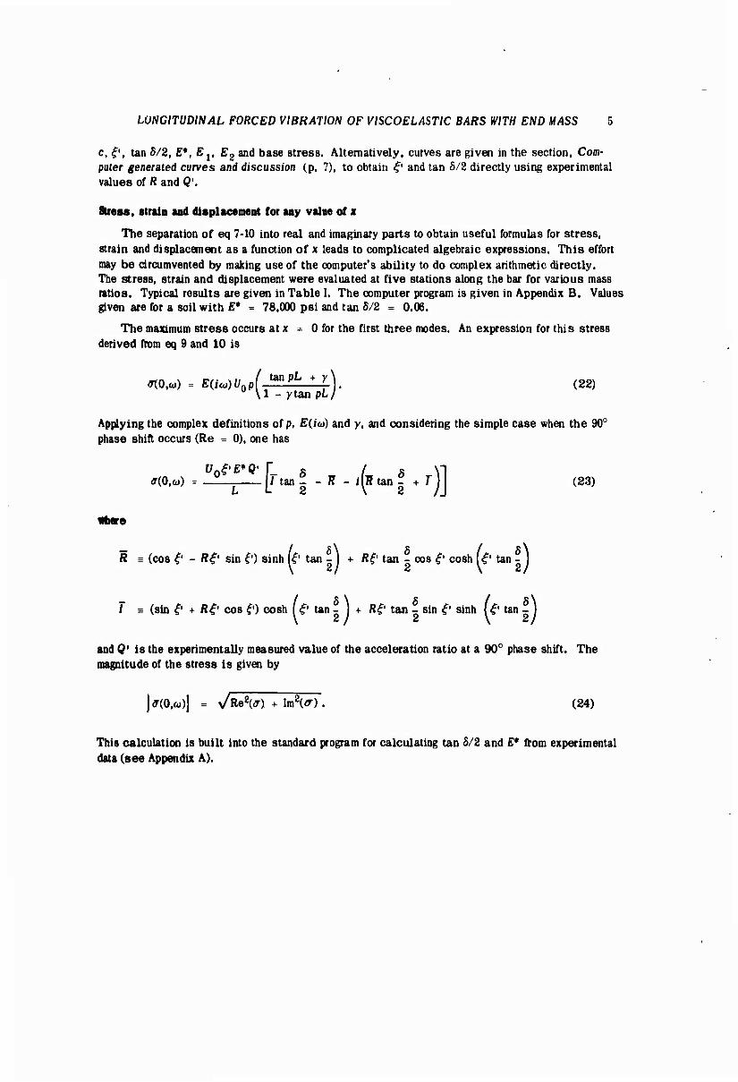
Stress, strain and displacement for any value of x

The separation of eq 7-10 into real and imaginary parts to obtain useful formulas for stress, strain and displacement as a function of x leads to complicated algebraic expressions. This effort may be circumvented by making use of the computer's ability to do complex arithmetic directly. The stress, strain and displacement were evaluated at five stations along the bar for various mass ratios. Typical results are given in Table I. The computer program is given in Appendix B. Values given are for a soil with E* = 78,000 psi and tan S/2 = 0.06.

The maximum stress occurs at x = 0 for the first three modes. An expression for this stress derived from eq 9 and 10 is

fftO.o) = E(Mt/0pfitanpL t l). (22)

\1 - ytan pL/

Applying the complex definitions of p, E(icj) and y, and considering the simple case when the 90° phase shift occurs (Re = 0), one has

Un£'E*Q' f- ä / ä M iriO.cj) = — [/ tan - - J? - j(R tan - + 7" 1 (23)

«here

R = (cos £ - /?£' sin f) sinh W tan - j + R£ tan - cos £ cosh f £' tan - j

I H (sin f1 + R^' cos f') cosh f^' ten - j + ß^1 tan - sin ^ sinh K" tan - j

and Q' is the experimentally measured value of the acceleration ratio at a 90° phase shift. The magnitude of the stress is given by

| (7(0,0))) = N/ReV) + ImV) . (24)

This calculation is built into the standard program for calculating tan £/2 and £♦ from experimental data (see Appendix A).

LONCITVDINAL FORCED VIBRATION OF VISCOELASTIC BARS WITH END »ASS

SI

I

?

I

I

^ en t«.

OB O W 00 -i t« ^ •-' o> 0> 9 S 2 2J *

■-' to *

« SJ N -<

<D ^ N 113 (O r» w o> « ra

S 81E: = ^

o >o 10 O 00

»H Si Ol

S8 888 0 es H W <-<

SS9So 8 S 9 * d

o •* CO ^ «ß 00 S $ <-<

»< -< en

§J -3 J J >/s e us o oi 2 c<- 5

c> o d o ^

<• eo «i •-< « g 2«S;S

8 52 • d 8

055a8 35 oo ^ ^

lO *-i *-• « r^

eo w «0 r- Q (M

sssss S £l 2 a *

o ^ » * * 88S

m f-i M n

^ on « oo N 01 lO N o

s s a a o'

O 00 US ) s t- to <A (0 ui n t^

§J J J J

d d ö d »<

o» ii a

«-• us co co SS1- 8

us go a> es CM oo ao us a» M

8 ^ e! ^ 8

o w t~ CO »Ä Ä ^8*

« K aj $ t- cs " N •-■ •-■

-H ^ 0» oi ^t -^ o> oo us 00 CD 0) ^ US 00 81 01 »< -i

O O « Q I> SS88

eo ^ OJ «

"< * r» «o o> M «o n

& SS8

O US 04 Oi OJ (M Tf Q W US * N *

§J J J J 8SS8

d d d d ^

eo II a


Redaction of theory to earlier work

For tan 5/2 = 0 eq 14 and 15 reduce to the equation for the eigenfrequencies of an elastic bar, i.e.

cot ^ = Rf (25)

as given by Timoshenko (195^).

For R = 0 (but including damping), eq 20 and 21 reduce to those given by Brown and Selway (1964), i.e.

f = J (2n - 1) (26)

and

•te) 2 sinh*

tan I = S^~L (27) 2 n(2n - 1)

where the notation has been changed to conform to this report. The latter two equations are similar to those given by Lee (1963) if the small angle assumption is made and only the first mode is considered.

COMPUTER GENERATED CURVES AND DISCUSSION

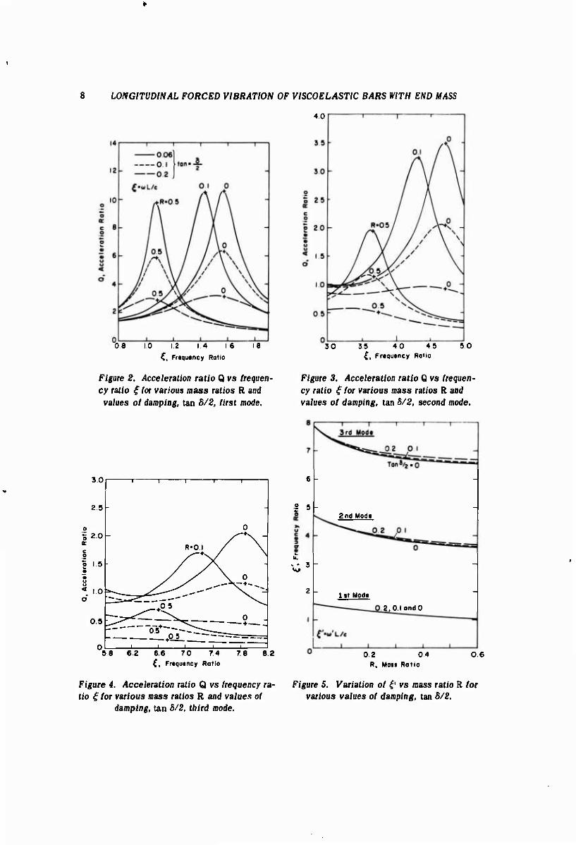
Response corves Q versos ( for three modes (Fig. 2-4)

Figures 2-4 give the absolute value of the acceleration ratio of the free end of the bar to the driven end (defined as Q) as a function of the frequency ratio £ for three modes of vibration. In generating these curves, tan 5/2 was arbitrarily set at a constant value for each curve although in a real material one would expect some variation with frequency. £ was incremented and values of Q and ^ were plotted for selected values of mass ratio R. In each mode the effect of end mass is obvious. The resonant frequency is lowered dramatically with increased R and there is also a decrease in Qmax. the maximum value of the response.

The computer plotter was programmed to print a plus sign on the Q versus ^curves (see Fig. 2-4 and Appendix C) when the phase relationship was 90°(corresponding to Re = 0), the convenient experimental point discussed in the section, Measurement of the complex modulus at 90° phase shift (p. 4). This point corresponds to specific values of £' and Q' also discussed previously. Un- less tan S/2 is very small, Q' does not coincide with Qmaz but is shifted to the higher frequency side of resonance. For the first mode with R 0, eq 20 reduces to cos £' = 0; hence ^ is n/2 for any value of tan S/2 as seen in Fig. 2. However, for R > 0 it is seen that £' actually in eases with increased tan 8/2 for a given mass ratio R although the true resonant frequency i. lowered with increased tan S/2. Experimenters must not confuse Qmax with Q'.

Variation of ? with R for various values of tan 8/2 (Fig. 5)

£' is an important quantity in the theory since it is used to compute the magnitude of the complex modulus E* using eq 16. Figure 5 is a computer generated plot of the variation of ^ with R for


4.0

08 10 12 14 16 18

C, Frequency Ratio

Figure 2. Acceleration ratio Q vs frequency ratio £ tor various mass ratios R and

values of damping, tan S/2, first mode.

30

2 5

o = 20 K

o 1.5

» 8 < 10 6

0.5

1 1 1 — T " I

0

R-OI / / \

/^+X \

y y/\ V 0

'^^—^1 ^:

^0

1 1 J ill

5 8 6 2 6 6 7 0 7 4 7 8 8.2 ^, Frequency Ratio

Figure 4. Acceleration ratio Q vs frequency ratio £ tor various mass ratios R and values of

damping, tan 8/2, third mode.

30 3 5 4 0 4 5 £, Frequency Ratio

50

Figure 3. Acceleration ratio Q vs frequency ratio £ for various mass ratios R and values of damping, tan S/2, second mode.

S 5

•*j 3 -

2nd Mode

1 tt Mode

2,0 land 0

02 04 R, Mat« Ratio

06

Figure 5. Variation of £' vs mass ratio R for various values of damping, tan 8/2.


various values of tan 5/2. £' decreases significantly with increased R especially for the higher modes. For any given value of R, £' increases with an increase of tan 8/2 as previously seen from Fig. 2. Fig. 5 was generated from eq 20; tan S/2 was specified and for an incremented value of R a half interval search method (see Kuo, 1965) was used to And and plot the values of £'. The oooputer program is given in Appendix D.

Tan 8/2 fron neasnred values of Q' for typical mass ratios (Fig. 6-8)

These curves permit the determination of tan 8/2 from experimentally measured values of Q' for selected values of mass ratio R. The computer program of Appendix A used to solve eq 20 and 21 was used to generate these curves.

These curves plot as a straight line on log-log paper down to a certain value of Q' (about 4.0 for the first three modes) and then show a slow deviation. This implies there exists a relationship over the linear range in dach mode of the form

Q' tan 8 I

C (28)

where the constant C is a different number for each value of R. It is easy to show from Fig. 6 or directly from eq 20 and 21 that for ß = 0 the constant in the first mode is n/2.

10

ronf oi —

CGI

1 r—i—i—i i i 11 -i 1—i—i i i i i

-j i i i i i i J 1 l i\k . i i 100

0', AcccKrotion Ratio

Figure 6. Tan 8/2 vs acceleration ratio Q', first mode.


10 -1 1—I—[ I I I I

_1 I I I I I I

0', Acc«l«rofion Ratio 100

Figure 7. Tan S/2 vs acceleration ratio Q1, second mode.

too 0', Acctlaration Ratio

Figure 8. Tan S/2 va acceleration ratio Q', third mode.


EXPERIMENTAL WORK

The experiment

The/Objective of the experimental work was to check the applicability of eq 20 and 21, which include the mass loading effect in the measurement of the dynamic modulus. To do this the theory of the section, Measurement of the complex modulus at 90° p/iase shift (p. 4), was employed using a polymer bar to simulate a soil sample.

The experiment consisted of driving the bar with a small end mass in the first three modes and measuring Q', the measured acceleration ratio, and /'. the frequency where the 90° phase shift occurred. The lest was then repeated with a larger end mass, with the bar shortened to maintain a constant frequency in each mode. The computer program of Appendix A was then used to compute E* and tan 5/2, both of which should be invariant with respect to mass ratio R since the assumption of the theory is that E* and tan S/2 are functions only of frequency and are independent of R. The check then was the coincidence of E* (or tan 5/2) measured at various mass ratios when plotted at the constant frequency.

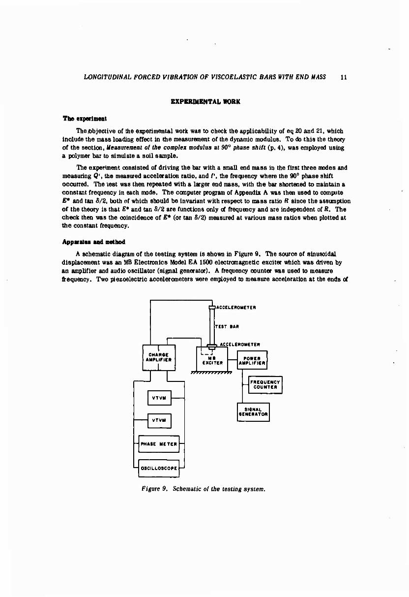
Apparatus and method

A schematic diagram of the testing system is shown in Figure 9. The source of sinusoidal displacement was an MB Electronics Model EA 1500 electromagnetic exciter which was driven by an amplifier and audio oscillator (signal generator). A frequency counter was used to measure frequency. Two piezoelectric accelerometers were employed to measure acceleration at the ends of

CHAROE AMPLIFIER

TT

1ACCELEROMETER

TEST BAR

, ACCELEROMETER

MB I I POWER EXCITER | lAMPUFIER

TTTTTTTT"^^

VTVM

VTVM

- PHASE METER -

"- OSCILLOSCOPE

FREQUENCY COUNTER

SIGNAL OENERATOR

Figure 9. Schematic of the testing system.


Brats Wtlght Vn" thü», l" diom H«x Socket Cap Scrtw

#8-32 »Vi" long

Cimant Eoilmon 910

Ttst Bar V«" diom

6 to 10" long

Tapptd for Stud #10-32« K»" long

Figure 10. Test specimen assembly.

the bar. The output from the accelerometers was fed into two charge amplifiers and read from two vacuum tube voltmeters. The amplified signals were displayed on a two-channel oscilloscope and the phase shift was observed on the oscilloscope. It was found that the phase of the two signals could be accurately measured on the oscilloscope; hence in the latter part of the experiment the phasemeter employed in earlier experiments was omitted.

The test specimens were %:in.-diam bars of low density polyethylene. The measured specific gravity of this material was 0.915. The bars were used as received from the supplier with no heat treatment and only the ends machined. All testing was done at 750F t 20F. The method of fasten- ing the end mass and fixing the bars to the exciter is shown in Figure 10. A 2-gram accelerometer was glued with Eastman 910 cement directly to the mass or in the case of the low mass tests directly to the free end of the bar. Bar lengths are given in Table II.

Calibration of the accelerometers was done at the three frequency ranges of interest (data were recorded in the first three modes) at the driving magnitude by driving the accelerometers back to back. Three different calibration constants were used. All tests were made with the exciter acceleration set at 10 G. Phase shift in the electronics was carefully checked. The transverse vibration of the bar was checked with a stroboscope and found to be insignificant. The signals showed no visible distortion.

AU data were recorded when the phase angle between the two signals was 90°. The value of Q' was measured and the frequency was recorded. £', tan 5/2, E*, E1, Eg and base stress were then computed using the computer program given in Appendix A. The experimental results are presented in Figures 11 and 12 and the computed results are presented in Table II.

LONGITUDINAL FORCED VIBRATION OF VISCOELASTIC BARS WITH END MASS

90,000

Modulus E (psi)

13

70.000

i i ■ 1 I r

I

I i I

. f . i 1 i I I 500 1000

Fraqutncy, Hz

a. End mass accounted (or.

5000

90,000

Modulus E (psi)

60,000

30,000 500

-

1 1 1 1 1

1

1 1

1 -

- f -

- Mots Rolio(R)Cod*

/ -

- • 0.029 AC 410 0 0 469 AC 436 • 0 414 00 904

■A -

1 1*1 1 1 1 1 1000 5000

Frtquancy, Hz

b. End mass neglected in theory.

Figure 11. Experimental results, E* vs frequency.

0.10

Ton | 005 -

500 1000 Fraquancy, Hz

a. End mass accounted for.

5000

0.15

Ton-2- 0.10 2

0.05 -

I 1 I 1 I Ma» Wielft) Csdf

— I I

• 0 029 4 0 410 • 0 0 489 AC 436 ■ 0 4 14 00 S04

\ • • * ( :

1 1 1 1 1 11 i

500 1000 Frtquoncy, Hz

b. End mass neglected in theory.

Figure 12. Experimental results, tan S/2 vs frequency.

5000


Table n. Computed results using experimental data.*

Mass Bar Frequency i4cce/ Frequency Test ratio length r ratio ratio E* ff. E, 00. R (in.) (Ht) Q' e Tan 5/2 (psi) (psi) (pai)

1 0.029 10.02 704 8.21 1.53 0.0771 72160 71302 11097 2 .029 10.02 2236 2.53 4.58 .0811 80843 79780 13067 3 .029 10.02 3842 1.66 7.64 .0711 85858 84989 12182

35 .029 10.00 712 10.25 1.53 .0619 73617 72954 9076 36 .029 10.00 2228 3.40 4.58 .0610 79952 79367 9737 37 .029 10.00 3830 2.12 7.64 .0568 84994 84446 9632 38 .029 10.00 3830 2.18 7.64 .0553 84995 84475 9384 39 .029 10.00 2215 3.34 4.58 .0621 79022 78413 9791 40 .029 10.00 707 9.68 1.53 .0655 72487 71866 9471 41 .029 10.00 718 9.71 1.53 .0653 74760 74123 9739 42 .029 10.00 2226 3.09 4.58 .0670 79807 79092 10659 43 .029 10.00 3839 2.05 7.64 .0586 85393 84807 9985 44 .029 10.00 702 9.83 1.53 .0645 71466 70871 9197 45 .029 10.00 2249 3.06 4.58 .0676 81460 80716 10982 46 .029 10.00 3882 2.03 7.64 .0591 87316 86706 10304 59 .489 7.00 722 12.42 1.08 .0476 73470 73139 6963 61 .414 8.25 2215 2.43 3.72 .0530 81364 80008 8600 62 .414 8.25 4067 0.91 6.65 .0526 86103 85626 9047 79 .504 6.69 738 12.50 1.08 .0471 71259 70943 6696 85 .410 8.25 3991 0.99 6.65 .0489 82887 82491 8089 86 .436 7.75 2326 2.33 3.70 .0539 80051 79685 8616

•^t, tan 5/2, E*, E,, and Ej were computed using the computer program of Appendix A.

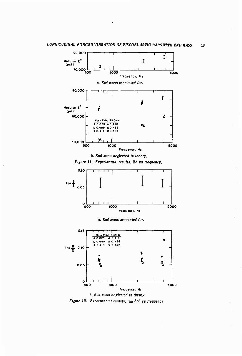
Experimental results

The ranges of E* and tan S/2 which were computed from the experimental values of Q' and /' for various mass ratios are shown in the upper portion of Figures 11 and 12, respectively, at the frequencies corresponding to the first three modes of vibration. To illustrate the errors introduced in computing the complex modulus ignoring end-mass effect, the lower halves of these figures are plots of the same data calculated from theory neglecting end-mass effect. All data are taken from Table II and there are seven points at each frequency (some are superimposed).

It may be concluded that large errors are introduced in the computation of E* if mass loading effects are neglected. For example, for R as low as 0.029, E* will be about 6% low in the first three modes; for ft = 0.5, E* will be about 50% of its true value in the first mode. This is illustra- ted graphically in Figure 11.

The effect of mass loading on the computation of tan S/2 is seen in Figure 13. The errors introduced using R = 0 theory are about 1% for R = 0.029 but become greater with increased mass ratio and mode number. For example. Young (1967) gives an error of 130.6% high for tan 8/2 for R m 0.414 in the third mode. The spread in the experimental data for tan S/2 for constant values of R makes it difficult to interpret the data in these tests.

CONCLUSIONS AND SUMMARY

The theory given here, including end-mass effect, leads to more nearly correct results in computing the complex modulus from vibrating bar test data and should be adopted. For laboratories


using the 90° phase shift measurement technique, this report presents curves that allow direct use of experimental data to calculate the complex modulus. For experimental data that fall outside the range of these curves, a computer program is presented for the same purpose.

LITERATURE CITED

Brown, O.W. and Sei way, D.R. (1964) Frequency response of a photoviscoelascic material. Experimental Uechunics, vol. 4, p. 57-63.

Kuo, S.S. (1965) Numerical methods and computers. Reading, Mass.: Addison Wesley.

Lee, T.M. (1963) Method of determining properties of viscoelastic solids employing forced vibration. Journal of Applied Physics, vol. 34, p. 1684-1589.

Scarborough, J.B. (1955) Numerical mathematical analysis. Baltimore: The Johns Hopkins Press, p. 803-804.

Timoshenko, S. (1955) Vibration problems in engineering, 3rd Ed. New York: D. Van Nostrand, p. 318-313.

Young, Wun-Chung (1967) Forced longitudinal vibration of a viscoelastic bar with end mass. University of New Hampshire, Master's Thesis.

17

APPENDIX A. TAN 5/2 AND E* FROM MEASURED Q' AND FREQUENCY

WH |T( (1,^1) 31 P[A[)(1,:) A,n.HO, AL.l-f ,N.UO

1 F-OPVA T ( 3r 1 o . 7 ,F- 1 0 . /i , I ^ . I',. r 10.-) I f ( M ) 1 , A 0 « 'l

'i HI = i ./r* C THF; rOLLOV.'ING 't ST A TF MrNT<-, AK". uSfO FO'^ CALCULATING THC C riPST TU I Al v.'.UJf" or LO^n FACTOP, DFL/?.

yrsi^-N E'fs-n.ono l PI =.T. I A 1 S9 x-Pi« e?. »xN-i. >/?. ÄS IN-Al Or. ( ( 1 . 4 S^PT ( 1 , +n-5«r) ) /H ) YrAS IM/y r,0 TO ( ? , 6 . 2 . 6 » ?» 6 ) t N

6 en = - n i r TM[ FOLLOWING 1 ^ T.T / 1 f M[ NT f. Apr F On THE ITCHATIONS

? SINHr (E:xP< X»Y )-EXP(-X»Y ) ) /? . CO.SHr (i:xf'( X«Y )+FxP{-X»Y ) ) /2. r i - coi.H« ( cc.( x > -A*X*:- i M( x ) ) < A«x«Y»r.05(X) »si NH

r?r5, INH* f SlNfXI +A*X*COr-. (X' ) ) -»COSH« A«.x«Y*r. 1N( xi-ni riyT?-ro--M*(-(i.+A)«siN(y)-A<x''(i.-Y*Y)«ror, (x)) FTXI ;:--rosn->( ( I, + A)»Y»SIN{X)+2.»A»X*Y*COS(X) ) KlX=5INH*((I,4Al«Y«COS(y)-2,«A«X«Y«S|N(X))+FlXT2 F2X = SINH« ( U .■» Al»COS(X)-A«X« < ! .-Y»Y J«51N<X) )+FaxT2 F 1 Y = 5: INH« ( ( 1 . +A HiX tCO:^ X) -A »Xi'X ■« r IN( X ) ) 4 COSH ;< A * X « X » Y «COS ( X ) FPyrCOSM« ( ( ! .+ A )*'/ »SIN(X) + A*X«X«CO<". ( X) ) +S IMHSA i X « K* Y * S I N ( X ) H-F I X«r?Y-F-'J y*F'2X HX = F 1 tf-?Y-F 2»F 1 Y MY-r?»Fiy-ri*r2x DF l.X-- -HX/H DFLY^-HY/H I F t AHS ( n' i v i -t Ps) ■-, s, i o

ci if c APS(iif i,v )-[ t\-,) .-»o.^r., i r; 1 0 X-- X-t 01 LX

Y- V-l or L Y r,o TO ?

30 PfLTA-2.vATAM(y) C- ( ,". «I1 I KLF*Al )/x PO: < PO^O.O.^fil ' ) /i^PtP-" \P,) FrPD -•' C«COS<r>tLTA/<-'. ) ) tip 11" 1 rF.*.COS (^n TA ) IF2 = f »S IN(UE l.TA )

C STWrSS CAL CUL AT ION' corr-uofx^FuvAt A fi - r> I N ( X ) 4 A»X * C O.^ ( X 1 n^ = COS( X )-A>:x'-S IN(X ) Cc. = A3X*Y

PF-AI I rF'^.tS INH-t C^'COSf X ) «r OSM AM i or, = A'•« r GSM4 c!''«s i M t \ i - s I \" i STPfSS = COr F ItSOWT ( ( AMI GC«Y-Pi ALL ) •;-»24 ( PC ALL «-Y4-AM ICG ) >«2 ) IC = C I r - F: v.'to 17r < 3 « 22 ) A . '<. i r . x . v , i ^ , i r , ; r-1 . I' ;•. STPf; ss . M CO TO 31

«■to CALL r: v n

18 APPENDIX A

21 FOPMAT ( 1 Ml .CX t I MH! «ftX. lHOt6X,f'iHr (CP'.) .'•<, «-tMV.'L /C./VX ♦6HT;<( L/?.r'X , IOKC( iN/src) «sx.6Hr.' (Pi-n .ox.rtif i. i ■:••.?HL'? »nx.6HM i.-' v,.'.>;. IflML OK MAP/)

?? roroMAT (rio.3»r3.?.2x. in.rx.r i: . *, i x ,f IO,/! ,^x. r v.^x, i7.rix, iv.^x, i i'ix.r i o.fi,' x.rc..? >

TYPICAL INPUT

^r, L r N mr-PL

o.o n.r>7 o.Pi i 13,0 0226"^ ni i .o-.-ir-or, 0.07lrvl B.^7 0."! I 1?.° 02?r>r> 01 1 .on-^ _,v, 0.0 ?^.6 0."1I 13.0 0663^ D? 0.07^r-n7 0.07153 ?f-.'') O."!! .-'.c> 06fOO 02 0,n7<-,r-07 0.0 17.^ 0."l 1 13.0 lO^iCJ 03 0.rv3^r-07 0.071'-.T I7.f> 0.°] 1 13,o 10"n3 03 1.f'3r.'- -0-?

TYPICAL OUTPUT

R C F(CPS) WL/C TCEL/2 C{ IN/SEC)

0.0 e.97 2269 1.571 o.o7cn 126156 0.C72 6.97 2269 l.ttt C.07C5 1 J51'.0 0.0 25.60 66 39 ^.712 O.COfl3 123012 0.072 25.60 6639 «.«ei 0.CÜ79 131567 o.o. 17.60 lC9fl3 7.851 0.C072 122130 0.072 17.60 1C9H3 7.369 0.C065 130160

Et PS II El E2 STRESS L OF M

1319692 1518817

1336218 1533538

190230 217226

2.691121 2.B9H1fll

13.90 13,90

1290213 1290065 21383 0.980596 13.90 1175233 1175017 23113 1.099321 13.90 1271209 1271076 18381 0.677136 13.90 1111012 1113921 1866 3 0.815897 1 3.90

19

APPENDIX B. STRESS, STRAIN AND DISPLACEMENT AS A FUNCTION OP X AND R (TABLE 1)

COMPLEX P,PL,C2.r,AMA, XI . LP5i, M GMA , D I SPL .Fi 1 C , QC . YC , EPS 1 100 REÄD(1.2) Y.UZ.O.AL.E . V.KOUNT

? fOPMAT(3F10.0,F10.^,r 10.0,Fin.^,12) IF (KOUNT )ri.7.?i)

5 WPITF(3,1) Y=2.»ATAN(Y) A 1 =X B|=ytTAN(Y/2.) nic=(o.o. i.o)«Bi PL-Al-BlC P=PL/AL f,AMArP#PL C2: (CSIN(PL )+GAMA<CCOS(PL ) )/(CCOSCPL )-GAMA«CSIN(PL > ) ZN=0.0

1 I A = ZN»X 0=A*TAN<Y/?.) nc=(o.o,i.n)*n XI =A-ÜC FPS = U7«P«(C?»CC0?( XI )-CSIN( XI )) YC=(0.0.1.0)«Y EPS I =FPS»CEXP(YC) SIGVAÊ»LEXP(YC jtfCPS HI fPL = U7»(CC0?( XI )+C?*CSIN( XI )-l.) DISPLSsCABSfUISPL) DI SPLW^PFLAl (DISPL ) oi SPL I =A iMAr-(r sr'L ) IFCOISPUPJ Ifi.lfi.IS

lf> nPHAr,r-0.n GO TO ??>

I r-. DPHA «-.F = A T AN ( D I SPL I /D I SPLP ) ?^ ÎGMAr, = CAHc,( SIGMA )

SIGMAPrREAL ( SIG./A ) S t GMAI=AI MAG(5 IGMA) IFCSIGMAPI 17,IB. 17

|7 .^PHA^-rr ATAN( ^ I i^MA I /S I r.v.'.ir ) in rps.c-=CAf»s(Fprii

FP.:;p=PEAL(rpS) EPS I-A I MAG(EPS) IF(EPr.P) l",rc'.!''

lo E PHASE:-A TAN (I pc, \ /f p.î. ) ?n K'ÎTF(.-?,.^) ri^PL.Î'Â,«-rx-, i

'».'PI T1" ( .T.?l ) 0 I'■PL.,- , niOÂ^, .rfJCir

U'P I TE ( .'',? I ) PPMA^.f , pPMA^P « FPHAf-F 7M-7N(+0.r'- IF ( 7N- I .?n ) M . i ,-'. ! ?

12 WR Iff ( 3i(>) GO TO 100

7 CALl T X IT 1 EOPf'AT ( IH1 «!<X, 1 ?HOI.ciPUArtM£ NT , .•'■'V .r,Hr TP« rS ,23X .6Hr. TP A I N/I 3 FOP-I AT ( /2r, i r..i .hx ..'T, i r,'.. v\ .;.'.' i r./. >

21 F- OPMA T ( r. 1 ? , /i , 1 2X , G 1 2. -"i . ! ?y . r. 1 7- . /i ) 6 FOPVAT(//) tl FO'.^'AT ( I « )

END

20 APPENDIX B

< oc

c er c

c c- c tC r-

s < rr c o ß a

Q Z UJ (1 a < a o u.

<

V

UJ et »-

c c c •

c

«0 c

< ^- < c

i

c L.

3 a ^- z ILI 2.

< a

Kl rn rt f0 (*l o o o

1 o o

1

UJ 1

UJ 1

UJ 1

UJ 1

UJ o ro 0» m <M •4 «N» •o «o * <*• f»> o <o r^ <M PX P>J IM« mt • • • • •

o 1

O 1

o 1

o 1

O 1

in m Ifl m in o i

UJ

o 1

o 1

o o 1

UJ 1

UJ i

UJ UJ (NJ o o o 00 oo ro CI m o 0> 00 * 00 ^ i-4 f\j m in ^ • • • • • o o o o o

m 1 \lf\ i dl i ro 1 w o o o o o i i 1 1 1

UJ UJ UJ UJ UJ -^ o« ^ 0- o m <a <o ro rsj — ir> <NJ fO f- Oi •o — «r •- •r «r fl * o •<■ ■c * - ^■ Oi t «M • <N . -< • -i •

o O O o o

o CO * 0> 0> CO ^ *4 0» o • • 1 • tr « ec <£ «M •

1 l 1 m4

1 00

1

•a r«. 1 ^ f> oo * o 1 l*\ •c f*S in ~ fst m •T

N * * m • i » • •

o o «■ w «» » O ^ m o o «o o O CS) « « i — ^ i - >r i o «» 1 »< ir\ J *• • in « in • vn v m

• «0 t «o • m t • • -. — •» t-i —1 r-l 00 —

1 s*1

<M PJ «M <9»l o o

1 O |

i UJ UJ

1 UJ

1 UJ

er oo w rg o w o in 0« ~4 <0 o>

o in *4 ^4 M^

• • • • • o o

1 o o o

•»■ m m fM (*> N tn IM o o

1 1 o

1 O ■

o 1

o 1

o 1 ■ 1 1

UJ UJ 1

UJ 1

UJ 1

UJ 1

UJ 1

UJ 1

UJ as * « •t CD O o oc %r lf\\~t — •C \f\ * 0>|* * o -< ro m.K m (M o> •* ^ -. ^• fM «0 * t- & ^r

o o o r- in t M1^ • rg -rf • OJ ~4 • • • • • • ^w • • -I • • -^ • • w4

o o o ? o o 1

o o o o i

o

21

APPENDIX C. Q VERSUS £ FOR VARIOUS R AND TAN S/2 VALUES (FIG. 2-4)

x o—r>jco—(\. o — fyoo—I\J -" ••••••• ••••••• C ooooooo ooooooo u a Q c

a O OOOCOPO (EfflOtCCCOO) u. •■••••• •••••••

nnnr>nnn tfi tfi tf> in lö tfl tf)

c

oco-J^^rifl^ooo-lnlPl^(^ • ••••••••••••••• uuoooooooooooooooo

I I X r Z c- z in "

0 o \ — uo o « ii u' O c • • c • V I • • — X X *M X X • • V V * V *. X o l/l r o m z c • o • o • n IJ l/l o u 0-, X » • • * » ♦ r o > y c >- > t 2 z • 2 2 *

<r • • < < r, • • < < X # <Vi (^ i- K • (V. tvi i- t- in c s \ * * c \ S * * • • « X X • X X M c M» A « 1 o -^ ^> » * V * > >- < • > > < < _1 ru z z + ♦ (^ 2 2 + ♦ • < 4 — M • « < ^ o h- t- — *» c H i- — -* z • * * X X * 4 » X X 4 o X X o X X 1- • 1 1 2 U! • 1 1 2 m I m O o o 9 ro • Q a Ifl u IM » a r l/l u N • o X X * * • (VJ X X » * .- * X • LJ u X X ^■ •» X • u L, X X « V X «0 in >■ + i « * M ** Ä • m > h + 1 * • 00 ivj ^ • • z «^ ^ < « * • N >- • z •— H A < «; » N > ß o < V >- 1 + * (Vi « • 2 co < * > V 1 + * .1 - • 2 I • h h z z ^ *- (\J w- N X < • t- f 2 Z ■» (VJ » M X < n • • <I < X X u. * • * t- in • —• < < X X h. (\J • • t- •~ • «•> • — X h t- 1- w w + M X o 9 -* — X • PJ o K K + X u * *« o x m o ffl « • O o * * oO 2 N — • u « a Ä u o • c 0 * * KT. 2 (VI IM • o < 1> o in • M 0- «i (T tm n X X o M ¥ o H o> ^ PH c- < tm » • X X O » o •— C r- • C W ■^ *- • ■ in u 1/1 * -» w *- <w W aM VM in V Ifl * « v w *» w .* M

h- K rj <« — ^• V* M Q ä M w -t E H 1- >0 »- 1- »- t- ^- — II II M a a M H 2 t- o K <1 H H t- I ll. o o • o tC II II C X X * )k L < 0 o 0 ki » u. o o o o c ■0 V — O X X » k u. tf O PM o u » U c in O "- - « J _l n • • • V M O u u I I w in J V* J D n 5 _J in J J J • • O in Li I T 1/1 ■M j D n 2 J wm J X krf W

o a a w •M o M • tl 2 H N * a M a 2 «# z L a a a ■H ü • IT o • V. 2 1- INI • ü M c. v -» a a u- 1- K 0- UJ *■ i t in o o M II o a S — L. o LJ o w 1 M <\ o II n c c \ M U. o — L. — o 4 <

- ii j j t- c « II ftj *rt + x X u t/l 0 • U, j II K _J K K h- -J K _i j _i 0 < II M ♦ i T o in 0 • u. —■ II 1- J h- 1- H j 1- j -1 S £ II U J _i — •i w £ X in z II n i0 M _i £ _i 2 «M 2 -1 _i j _i c v 1 X cl 2 II n in ~ J >; J 2 •- 2 j j _l a B: c u u < < er UJ u. < o o II o ^ M ftj II II b. < «I o < C a 0 < o < < < tu u. < O o 0 fi. M II u. <: < o < o a O 4 o < ■I o o 2 - - (J o 3 IT in O 0 X u irt u. L. N N u in o u VJ » o U o u u u s Kl 0 o X u in u. L. N N u in o u u 3 U o o u u li. L. kl

in B M « o in (>■ in 01 <\j c o IT CiJ

^ (VJ >0

23

APPENDIX D. ^ VERSUS R FOR VARIOUS VALUES OF TAN 8/2 (FIG. 5)

IC = 1

DO 11 1=1,2 READ(1.22)

11 WR1TE(3.22) 22 FORMAT(IX.VgH

I ) EPS=0.001 CALL PLOT(ic.o.o.o.6.6.o.ri,i.n.ri.io.o.io,o.i.O)

CALL PLOT(99) 30 READ(I.3) Xll,x22,V.fJ

IF(Xll) 6.7.6 6 WRITEO.«) N

R=-0.00125

DO 25 K=l.6 DO 10 1=1.SO Xl=Xl 1 X2=X22 R=R+0.00125 PI=3.14159 C0T1=C0S(X1 )/5IN(XI ) C0T2 = C0r>(x2)/SIN(X?) FX1=C0T1-R«X1+R»X1«Y«C0T1*TANH(X1«Y) FX2sC0T2-R»X2 + R»X2«Y*C0T.?»TANH<X2«V I

70 X^(Xl+X2)/2. CO X = COS(X)/5.IN(x ) FX-C0TX-R*X+R«X«Y»COTX«TANH(X»Y) IF(AD5(rX)-EPr,) 15,15.60

60 1F(FX»FX1) 50,15,80 50 X2=X

FXSsFX GO TO 70

80 XI=X FX1=FX GO TO 70

15 CALL PLOT( ICCR.X) 10 COMTINur

WR1TF(3.1) Y.R.X

25 CONTINUE CALL PLOT(99) GO TO 30

7 CALL PL.0T( 100) CALL EXIT

1 FORMAT(OF 10.5) 3 FORMAT(3F10.5.12) 4 FORMAT (//"JX,4HN = ,12//) CNÜ

C DATA f OR APPfNllIX I i PRor.

C Y R X

o.n 1.8 0.0 01 o.n I.Q 0. 1 01 O.P 1.0 0.2 01 3.4 5.0 0.0 02 3.4 5.0 0.1 or 3.4 5.0 0.2 0," 6.5 9.0 0.0 0 1 6.5 9.0 0.1 OT 6.5 P.O 0.2 03 0.0

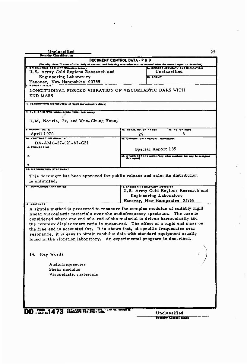
Unclassified 25 ^•curit^ClMjificjtloi^

DOCUMENT CONTROL DATA .R&D (Sieurlty clmttlllcmllan of llll; body ol mbiltmcl mod Indtulng amouilon mufl *« «iHf< whm> U— mmmU nßotl I« tlattHM}

I. ORieiNATINO ACTIVITY CCoipOMM «utflor; U.S. Army Cold Regions Research and

Engineering Laboratory Hanover. New Hampshire 03755

aa. McronT ■■cuniTv CLAMIFICATION

Unclassified ab. anouP

1. REPORT TITLK

LONGITUDINAL FORCED VIBRATION OF VISCOELASTIC BARS WITH END MASS

I (Typ* ol fpott and lnclu»lw dml0»)

%■ AUTHORII) (Flm nrnrn», mIBi Inlllal, fad naaM; / *

D.M. Norris, Jr. and Wun-Chung Young

«■ RKRORT DATS

April 1970 »«. TOTAL NO. or RAac*

29 7*. NO. OP RIP«

M. CONTRACT OR ORANT NO.

DA-AMC-27-021-67-G21 *. PROJECT NO.

M. ORiaiNATOR'I REPORT NUhfSERC«)

Special Report 135

IhU—tott) »1*1 (Any otift numbtn Mai may k» aaaffnatf

10. DIITRiaUTION (TATEMENT

This document has been approved for public release and sale; its distribution is unlimited.

II. SUPPLEMENTARY NOTEI It. (PONtORINS MILITARY ACTIVITY

U.S. Army Cold Regions Research and Engineering Laboratory

Hanover, New Hampshire 03755 I*. A.ITRAAT

A simple method is presented to measure the complex modulus of suitably rigid linear viscoelastic materials over the audiofrequency spectrum. The case is considered where one end of a rod of the material is driven harmonically and the complex displacement ratio is measured. The effect of a rigid end mass on the free end is accounted for. It is shown that, at specific frequencies near resonance, it is easy to obtain modulus data with standard equipment usually found in the vibration laboratory. An experimental program is described.

14. Key Words

Audiofrequencies Shear modulus Viscoelastic materials

DD MST*AA73 •A*". DO PONM I4T». I JAM M, «MICH I* worn AMMV «*•■. Unclassified

••curity Claaaiflcalloa

longitudinal forced vibration of viscoelastic … · computer generated curves and discussion 7 ......

Documents