mba super notes: statistics: descriptive measures

MBA Super Notes © M S Ahluwalia Sirf Business

Version 1.0

Descriptive measures

http://sirfbusiness.blogspot.in/search/label/Super-Notes

http://msahluwalia.blogspot.com/

http://sirfbusiness.blogspot.com/


MBA SUPER NOTES

Statistics





Disclaimer !

Copyright © 2014, by M S Ahluwalia Trademarks: Super Notes, Sirf Business and the MSA logo are trademarks of M S Ahluwalia in India and other countries, and may not be used without written permission. All other trademarks are the property of their respective owners. M S Ahluwalia, is not associated with any product or vendor mentioned in this book. Limit of liability/disclaimer of warranty: The publisher and the author make no representations or warranties with respect to the accuracy or completeness of the contents of this work and specifically disclaim all warranties, including without limitation warranties of fitness for a particular purpose. This book should not be used as a replacement of expert opinion. No warranty may be created or extended by sales or promotional materials. The advice and strategies contained herein may not be suitable for every situation. This work is sold with the understanding that the publisher is not engaged in rendering legal, accounting, or other professional services. If professional assistance is required, the services of a competent professional person should be sought. Neither the publisher nor the author shall be liable for damages arising herefrom. The fact that an organization or website is referred to in this work as a citation and/or a potential source of further information does not mean that the author or the publisher endorses the information the organization or website may provide or recommendations it may make. Further, readers should be aware that internet websites listed in this work may have changed or disappeared between when this work was written and when it is read. This document contains notes on the said subject made by the author during the course of studies or general reading. The author hopes you will find these ‘super-notes’ useful in the course of your learning. In case you notice any errors or have any suggestions for the improvement of this document, please send an email to [email protected]. For general information on our other publications or for any kind of support or further information, you may reach us at http://SirfBusiness.blogspot.com.




mailto:[email protected]




Numerical Descriptive measures

4

Measures of central tendency/ location

Mean and its types

Measures of location

Mode

Measures of dispersion/ variation

Range and IQR

Mean and standard deviation

Coefficient of variation

Measures of shape/ symmetry

Skewness Kurtosis

Numerical descriptive measures

• Large data sets can often be adequately described by just a few numbers: • Populations are described by parameters. The symbols are notated by

Greek symbols, or upper case English symbols • Samples are described by statistics. The symbols are notated by lower

case English symbols • Populations and parameters are seldom encountered in the real world,

therefore, it would be worthwhile to focus attention on samples and statistics

Types of descriptive measures





Interpreting histograms (1/2)

5

Interpreting histograms

• The main reason for drawing a histogram is to graphically summarize the data.

• We can also use the histogram to understand the data. Following are some things to look for in a histogram: • Patterns

• Is there an overall pattern, and any striking deviations from that pattern • Overall pattern of a distribution • Look for the center of the distribution • Look for the spread of the distribution

• Does the distribution have a simple shape that you can describe in a few words

• Outliers • any individual observation that lies outside the overall pattern of

the graph





Spread

Shape

Interpreting histograms (2/2)

6

05

101520

0-4

>4-8

>8-1

2

>12

-16

>16

-20

>20

-24

>24

-28

>28

-32

>32

-36

>36

-40

Peaked distribution

0

5

10

15

20

0-4

>4-8

>8-1

2

>12

-16

>16

-20

>20

-24

>24

-28

>28

-32

>32

-36

>36

-40

Skewed to the left (-ve skew)

0

5

10

15

20

1 3 5 7 9

11

13

15

17

19

Bimodal distribution

0

5

10

15

0-4

>4-8

>8-1

2

>12

-16

>16

-20

>20

-24

>24

-28

>28

-32

>32

-36

>36

-40

Skewed to the right (+ve skew)

05

101520

0-4

>4-8

>8-1

2

>12

-16

>16

-20

>20

-24

>24

-28

>28

-32

>32

-36

Flat distribution





Measures of central tendency/

location

1

7





Measures of Central tendency

8

1

Mean

Arithmetic mean

Harmonic mean

Geometric mean

Measures of location

Median Quartiles Deciles Percentiles

Mode

Measures of central tendency

• Indicates a number, which all the observations tend to have, or a value where all the observations can be assumed to be located or concentrated (center of a distribution)

Use • Gives a single value that is representative of the distribution i.e. gives us some idea of what the ‘average’ or ‘middle’ or ‘most occurring’ number in the data set is

• Facilitates comparison of: • One sample at different points of time • More than one sample at a point of time

• It is analogous to the concept of center of gravity • It is the most common measure used to describe data sets

Types





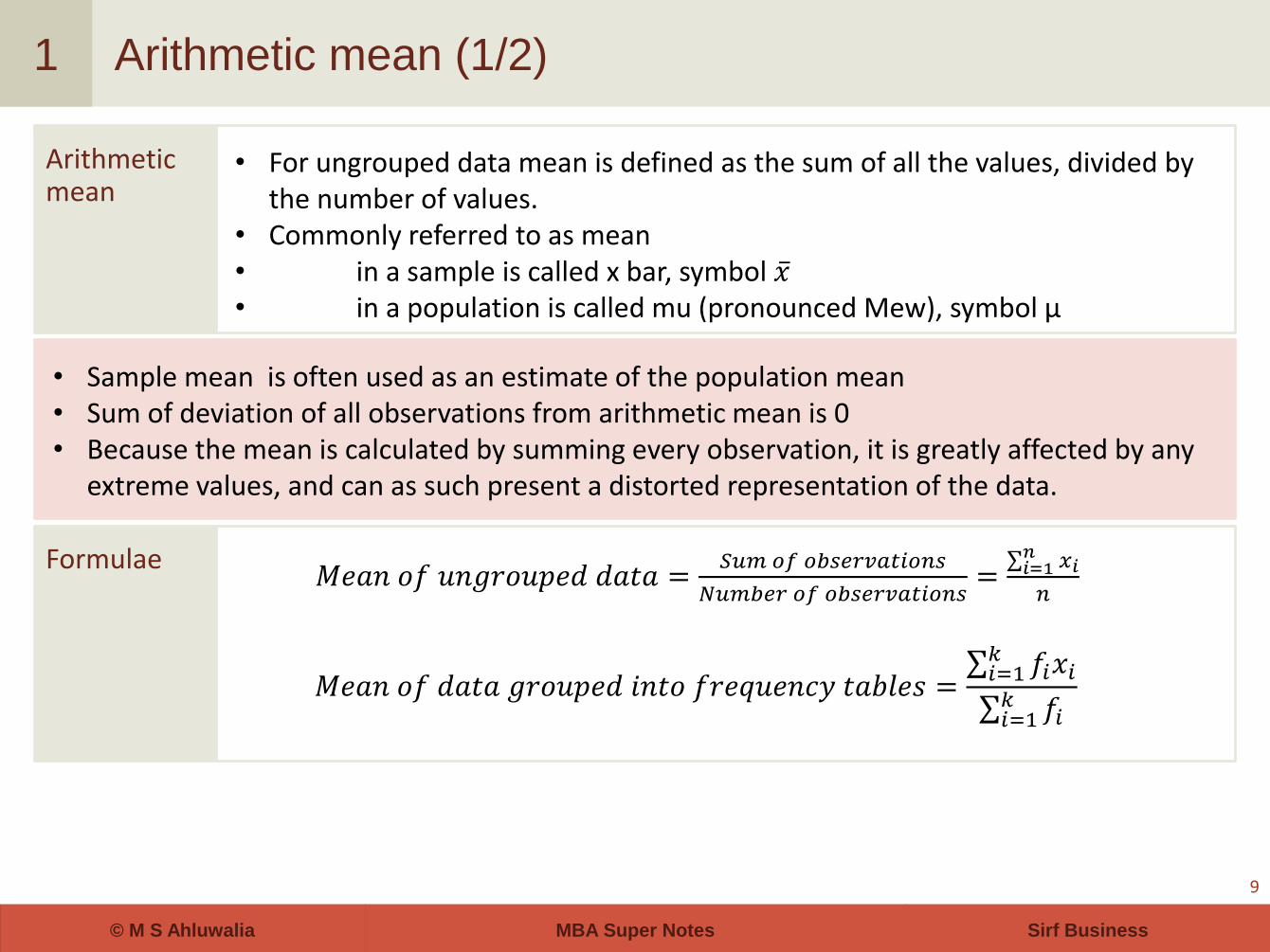
Arithmetic mean (1/2)

9

1

Arithmetic mean

• For ungrouped data mean is defined as the sum of all the values, divided by the number of values.

• Commonly referred to as mean • in a sample is called x bar, symbol 𝑥 • in a population is called mu (pronounced Mew), symbol μ

• Sample mean is often used as an estimate of the population mean • Sum of deviation of all observations from arithmetic mean is 0 • Because the mean is calculated by summing every observation, it is greatly affected by any

extreme values, and can as such present a distorted representation of the data.

Formulae 𝑀𝑒𝑎𝑛 𝑜𝑓 𝑢𝑛𝑔𝑟𝑜𝑢𝑝𝑒𝑑 𝑑𝑎𝑡𝑎 =

𝑆𝑢𝑚 𝑜𝑓 𝑜𝑏𝑠𝑒𝑟𝑣𝑎𝑡𝑖𝑜𝑛𝑠

𝑁𝑢𝑚𝑏𝑒𝑟 𝑜𝑓 𝑜𝑏𝑠𝑒𝑟𝑣𝑎𝑡𝑖𝑜𝑛𝑠= 𝑥𝑖𝑛𝑖=1

𝑛

𝑀𝑒𝑎𝑛 𝑜𝑓 𝑑𝑎𝑡𝑎 𝑔𝑟𝑜𝑢𝑝𝑒𝑑 𝑖𝑛𝑡𝑜 𝑓𝑟𝑒𝑞𝑢𝑒𝑛𝑐𝑦 𝑡𝑎𝑏𝑙𝑒𝑠 = 𝑓𝑖𝑥𝑖𝑘𝑖=1

𝑓𝑖𝑘𝑖=1





Arithmetic mean (2/2)

10

1

Change of origin

• When a number, say M, is subtracted from each observation then it shifts the origin from 0 to point M

• Mean of original data = Mean of new observations + M (origin)

Change of scale

• When the original observations are scaled or divided by a number to reduce the value of original observations

• Mean of original data = Mean of new observations x Factor by which observations were divided

Change of both origin and scale

• Origin of variable shifted to M and observations are scaled by a factor, say N • Mean of original data = M + (N x Mean of new observations)





Median

11

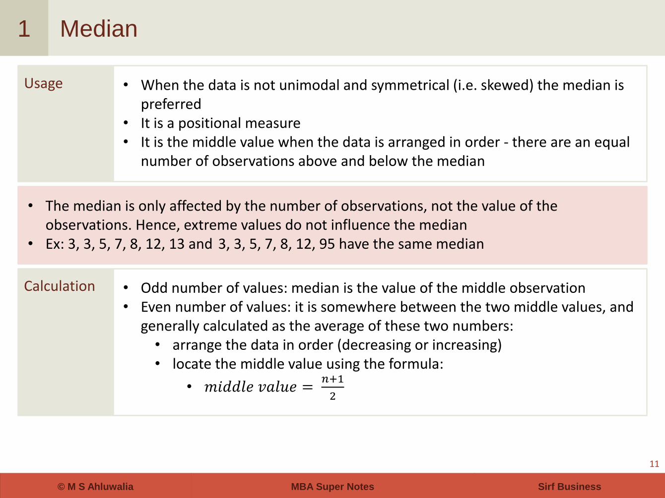
1

Usage • When the data is not unimodal and symmetrical (i.e. skewed) the median is preferred

• It is a positional measure • It is the middle value when the data is arranged in order - there are an equal

number of observations above and below the median

Calculation • Odd number of values: median is the value of the middle observation • Even number of values: it is somewhere between the two middle values, and

generally calculated as the average of these two numbers: • arrange the data in order (decreasing or increasing) • locate the middle value using the formula:

• 𝑚𝑖𝑑𝑑𝑙𝑒 𝑣𝑎𝑙𝑢𝑒 = 𝑛+1

2

• The median is only affected by the number of observations, not the value of the observations. Hence, extreme values do not influence the median

• Ex: 3, 3, 5, 7, 8, 12, 13 and 3, 3, 5, 7, 8, 12, 95 have the same median





Mode

12

1

Mode • The mode is the value(s) in the distribution with the maximum frequency – the most common observation in the series

• Useful on nominal scale data, where it is not possible to calculate the mean or median

• A distribution can have more than one mode (e.g. two modes = bimodal) • Does not necessarily indicate the centre of a distribution – mode may even

be a class interval rather than a data value

Examples

0

5

10

15

20

1 3 5 7 9

11

13

15

17

19

Bimodal distribution

0

5

10

15

0-4

>4-8

>8-1

2

>12

-16

>16

-20

>20

-24

>24

-28

>28

-32

>32

-36

>36

-40

Skewed to the right

modes = 5 and 16 mode = >8 - 12





Comparison of mean, median & mode

13

1

If data is uni-modal and symmetrical, the three measures of central tendency will be of similar value

If data is skewed, mean and median will not be equal. The mean will be ‘pulled towards the skew’.

The mode acts similarly, but not always.

Skewed to the right or +ve skew: Mean > Median > Mode

• Skewed to the left or -ve skew: Mean < Median < Mode

*Right and left refers to the side of the long tail





Measures of Dispersion

2

14





Measures of Dispersion

15

2

Range Variance Standard deviation Coefficient of

variation

Measures of dispersion

• Indicate the extent to which the observations differ from each other

Major types of measures of dispersion





Range

16

2

Range • It is the difference between the maximum and minimum observations in a data set:

𝑅𝑎𝑛𝑔𝑒 = 𝑥𝑚𝑎𝑥 − 𝑥𝑚𝑖𝑛

• Usually the actual values are given. For example; “Chocolate prices ranged between $1 and $1.5 per bar during 2014”

• It gives no indication of the dispersion of values between these two extreme values, i.e., there may be a lot of values clumped at either end of the distribution

Q1 Q3 M Lowest number

Highest number

Range

Inter Quartile Range





Variance

17

2

Variance • Variance and standard deviations are the two commonly used measures which take into account all data values

• A data set that is more variable will have a larger variance than a data set that is relatively homogeneous

• Variance is the sum of the squared deviations divided by the number of observations

Calculation • Calculate deviation - distance of each observation from the mean = 𝑥𝑖 − 𝜇 • Square the deviations = (𝑥𝑖−𝜇)

2 • Sum the squared deviations and divide by number of observations to get the

variance • The variance is hence the average squared deviation of the data

Formulae • For a population, variance is notated by 𝜎2

𝜎2 = (𝑥𝑖−𝜇)

2𝑁𝑖=1

𝑁

• For a sample, variance is notated by 𝑠2:

𝑠2 = (𝑥𝑖−𝑥 )

2𝑛𝑖=1

𝑛 − 1





Standard deviation

18

2

Standard deviation

• Absolute measure of the deviation of the observation from its arithmetic mean

• Also known as the Root Mean Square (RMS) value

Calculation • The standard deviation is simple the +ve square root of the variance. Hence for a population the standard deviation is s and σ for a sample, i.e., the standard deviation is in the same units as the mean.

Formulae Population:

𝜎 = 𝑣𝑎𝑟𝑖𝑎𝑛𝑐𝑒 Sample:

𝑠 = 𝑥𝑖 − 𝑥

2𝑛𝑖=1

𝑛 − 1





Coefficient of variance

19

2

Coefficient of variance (CV)

• It is a relative measure of variability which has no units • It expresses standard deviation as a proportion of arithmetic mean • It is used for comparing data that are not measured using the same units, or

when comparing data with significantly different means • The CV can only be calculated on data collected at the ratio level

Formulae Population:

𝐶𝑉 =𝜎

𝜇

Sample:

𝐶𝑉 =𝑠

𝑥





Quartiles

20

2

Quartiles • Quartile is a positional measure like median (calculation is also similar) • There are three quartiles that divide the distribution into four equal parts:

• The first quartile lies one quarter of the way through the data, i.e., 25% of the observations are less than the first quartile

• The second quartile (median) is the middle value of the data set, i.e., the value that 50% of observations are greater than and 50% of observations are less than the second quartile

• The third quartile lies three quarters of the way through the data, i.e., three quarters of the data values are less than the third quartile

Inter quartile range

• The difference between the 1st and 3rd quartiles is called the Inter Quartile Range

• It signifies the central 50% of the observation

0

5

10

15

20

25

30

35

37

5

42

5

47

5

52

5

57

5

62

5

67

5

72

5

77

5

82

5

87

5

92

5

97

5

10

25

Fre

qu

en

cy

Salary midpoint ($)

Company weekly salaries





Percentiles

21

2

Percentiles • Positional measure like median and quartiles • There are 99 percentiles in a distribution. They divide the data into 100 equal

parts





Five Number Summary

22

2

Five number summary

• Quartiles, median and range can be used collectively to determine the five-number Summary

• It offers a reasonably complete description of the centre and the spread of the data around the centre





Boxplots

23

2

Boxplots • The five number Summary lends itself nicely to a new type of graph, the boxplot

• With boxplots it is imperative that the plot is drawn OFF the axis, that the axis is drawn to scale and clearly labelled with units.

• The plot itself should have a clear title attached. • They can be drawn either vertically or horizontally • Different computer programs use different methods for generating boxplots:

• Most programs like to identify outliers in the data - usually any observation(s) that are more than 1.5 Inter Quartile Ranges from 1st or 3rd quartile

Use • Boxplots allow the viewer to easily assess the range, spread and centre of a distribution

• They are useful for comparing more than one distribution (better than histograms or stem leaf displays)

Q1 Q3 M min max





Approximate statistics for grouped data

24

2

Statistics for grouped data

• When data is given in a frequency distribution table, we cannot calculate the exact mean and standard deviation

• However, it is possible to calculate the approximate mean and variance

Formulae • Mean

𝑥 ≅ 𝑓𝑖𝑥𝑖𝑘𝑖=1

𝑛

• Variance

𝑠2 ≅1

𝑛 − 1 𝑓𝑖𝑥𝑖

2 − 𝑛𝑥 2𝑘

𝑖=1





The Empirical rule

25

2

The empirical rule

• The great benefit of standard deviation is that in certain circumstances it allows us to calculate the number of observations lying within particular intervals of the distribution

• The Empirical rule evolved from studies involving ‘mound’ shaped distributions like the following:

• If a sample (or population) of measurements has a mound shaped distribution: • approximately 68 % of observations lie within one standard deviation of

the mean • approximately 95 % of observations lie within two standard deviations

of the mean • approximately 99.7 % of observations lie within three standard

deviations of the mean

99.7 %

68 %

95 %





Measures of Shape

3





Skewness

27

3

Definition

• Measure of asymmetry of a frequency distribution

• It measures the deviation of the distribution from a symmetrical uniform bell shaped curve

Types

• Following are the 3 possibilities: • Skewed to left (negatively

skewed)

• Mean < Median < Mode

• Symmetric or unskewed

• Mean = Median = Mode

• Skewed to right (positively skewed)

• Mean > Median > Mode

Formulae

• Bowley’s coefficient of skewness to measure extent of skewness

• Varies from -1 to +1

• Positively skewed >0

• Negatively skewed <0

• Pearson’s measure of skewness

0

2

4

6

1 2 3 4 5 6

(Q3 − Med ) – ( Med – Q1 ) Sk = −−−−−−−−−−−−−−−−−−−−−−−−−−−−−−−−

2 Q2 or ( Q3 − Q1)

0

2

4

6

1 2 3 4 5 6

0

2

4

6

1 2 3 4 5 6

= Mean −Mode

𝜎

= 3 (Mean − Median)

𝜎





Kurtosis

28

3

Definition

• Measure of flatness or ‘peaked-ness of a frequency distribution

• Also known as ‘Convexity of the curve’

Types

• Platykurtic (relatively flat distribution)

• Mesokurtic (not too flat, nor too peaked distribution)

• Leptokurtic (relatively peaked distribution)

0

2

4

6

8

1 2 3 4 5 6 7

0

2

4

6

8

1 2 3 4 5 6 7

0

2

4

6

8

1 2 3 4 5 6 7





Standardised variable

4





Standardised variable

30

4

Calculation Standardised variable, Where:

x = variable m = mean σ = standard deviation

Definition • A variable whose origin is shifted to its arithmetic mean and which is then scaled by its standard deviation

• Standardized variable has Mean = 0 and Standard deviation = 1

• It is also known as ‘Standardised Score’

z =x − m

σ





Do you have any questions or some feedback to share?

Send an email to

[email protected]

Thank You!

31




mailto:[email protected]


M S Ahluwalia, is a top B-School graduate (MBA, Finance), CAIIB & JAIIB (both with ‘First class with

Distinction’) and ex-Banker from India.

He’s also a visual artist, blogger, designer and photographer. To know more please visit Estudiante De La

Vida or follow on Twitter or Facebook:

For more Super-Notes: Click Here











http://sirfbusiness.blogspot.com/search/label/Super-Notes




http://twitter.com/msahluwalia

http://www.facebook.com/pages/M-S-Ahluwalia/258015240783