! "#$%&&#&'()(#*

+,.-/01% 2

34(#6572%1#*8 ,9:-<;6->=72?@#

3A22* , %&2B&6572%1#*) ,9:-DCE>(%F

572%1#*8 , G AHI#F2*J KL2KFM;N@OP#)7QRTSUVSW

9X1O/&#)12?$G AL&)*8K*34(#6572%1#*8 ,

Y O#0WS(RTS

Z

Maximum Smoothed Likelihood for Multivariate

Mixtures

Michael Levine, David R. Hunter∗, Didier Chauveau

April 15, 2010

Abstract

We introduce an algorithm for estimating the parameters in a fi-nite mixture of completely unspecified multivariate components in atleast three dimensions under the assumption of conditionally indepen-dent coordinate dimensions. We prove that this algorithm, based on amajorization-minimization idea, possesses a desirable descent propertyjust as any EM algorithm does. We discuss the similarities betweenour algorithm and a related one—the so-called nonlinearly smoothedEM, or NEMS, algorithm for the non-mixture setting. We also demon-strate via simulation studies that the new algorithm gives very similarresults to another algorithm that does not satisfy any descent algo-rithm, thus validating the latter algorithm, which can be simpler toprogram. We provide code for implementing the new algorithm in apublicly-available R package.

Keywords: EM algorithms, MM algorithms, NEMS, nonparametricmixtures

1 Introduction

Suppose the r-dimensional vectors X1, . . . ,Xn are a simple random samplefrom a finite mixture density of m components f1, . . . , fm, with m > 1 andknown in advance. It is assumed throughout this manuscript that each oneof these densities fj is equal with probability 1 to the product of its marginaldensities:

fj(x) =

r∏k=1

fjk(xk) (1)

This, in turn, means that, conditional on knowing the particular subpopu-lation the observation Xj came from, its coordinates are independent. This

∗Corresponding author. Address: Department of Statistics, Pennsylvania State Uni-versity, University Park, PA 16802, USA. dhunter@stat.psu.edu

1

conditional independence assumption has appeared in a growing body ofliterature on non- and semi-parametric multivariate mixture models; seeBenaglia et al. (2009b) for a discussion of the relevant literature.

We let θ denote the vector of parameters, including the mixing pro-portions λ1, . . . , λm and the univariate densities fjk. Here and throughoutthe article, j is the component index and k indexes the coordinate. Con-sequently, 1 ≤ j ≤ m and 1 ≤ k ≤ r. Therefore, under the assumptionof conditional independence, the mixture density evaluated at the pointxi = (xi1, . . . , xir)

> can be represented as

gθ(xi) =m∑j=1

λj

r∏k=1

fjk(xik), (2)

where λ = (λ1, . . . , λm) must satisfy

m∑j=1

λj = 1 and each λj ≥ 0. (3)

The question of identifiability of the parameters in Equation (2) is ofcentral theoretical importance. By identifiability, we refer to the question ofwhen gθ uniquely determines λ and each of the fjk, at least up to so-called“label-switching” and any changes to the densities fjk that occur on a setof Lebesgue measure zero that do not therefore change the distributions Fjk(here, “label-switching” refers to permuting the order of the summands, 1through m, in equation (2)). Hall and Zhou (2003) established that whenm = 2, identifiability of parameters generally follows in r ≥ 3 dimensionsbut not in fewer than three. However, a general result for more than twocomponents proved elusive, though several articles on the topic appeared inthe literature (e.g., Hall et al., 2005; Kasahara and Shimotsu, 2008). Then,Allman et al. (2009) finally proved an elegant and powerful result using atheorem of Kruskal (1977), establishing the identifiability of the parametersin (2) whenever r ≥ 3, regardless of m, under weak conditions. To wit, theidentifiability follows as long as for each k, the density functions f1k, . . . , fmkare linearly independent (except possibly on a set of Lebesgue measure zero,of course).

An EM-like algorithm designed to estimate θ in model (2) was intro-duced in Benaglia et al. (2009b). That algorithm can handle any number ofmixture components and any number of vector coordinates of the multivari-ate observations, unlike other existing algorithms. It also yields considerablysmaller mean integrated squared errors than an alternative algorithm (Hallet al., 2005) in a simulation study. However, despite its empirical success,this algorithm lacks any sort of theoretical justification; indeed, it can only

2

be called “EM-like” because it resembles an EM algorithm in certain as-pects of its formulation. The current article corrects this shortcoming byintroducing a smoothed loglikelihood function and formulating an iterativealgorithm with a provable monotonicity property that happens to produceresults in that resemble those of Benaglia et al. (2009b) in practice.

The association of EM algorithms with mixture models has a long his-tory; indeed, the original “EM algorithm” article—i.e., the article in whichthe initials “EM” were coined, not the first appearance of such an algorithm—describes a finite mixture model as one of several EM examples (Dempsteret al., 1977). Not long after, a sizable literature on “nonparametric mix-tures” appeared (see, e.g., Lindsay, 1995), but here, “nonparametric mix-tures” was used in a different sense: The mixing distribution, rather thanthe component densities, were assumed to be unspecified (by contrast, thecurrent article and most of the literature we have cited so far assume themixing distribution to have finite support with a fixed cardinality, but thecomponent densities are unspecified). For this distinct concept of nonpara-metric mixture models, Vardi et al. (1985) introduced an EM algorithm formaximum likelihood estimation of the mixing distribution.

The Vardi et al. (1985) algorithm has an elegant convergence theoryassociated with it, but unfortunately it does not deal with ill-posedness ofthe problem. To overcome this difficulty, Silverman et al. (1990) proposedthe EMS (Smoothed EM) algorithm that smoothes the result of each step ofthe classical EM algorithm. The practical performance of this algorithm isexcellent but, unfortunately, understanding its quantitative properties hasturned out to be a difficult issue. Eggermont (1992) first proposed the idea ofusing a regularization approach to modify the EMS algorithm in such a waythat the resulting algorithm is easier to investigate theoretically. Eggermontand LaRiccia (1995) showed that the resulting NEMS (Nonlinear EMS)algorithm is, indeed, an EM algorithm itself and that its convergence theoryis very similar to that of the original EM algorithm introduced in the mixingdensity estimation context by Shepp and Vardi (1982). Eggermont (1999)showed that it also possesses a descent property and that the correspondingmaximum likelihood problem has a unique solution. Finally, it is knownthat the practical performance of the NEMS algorithm is at least as goodas that of the EMS algorithm; again, see Eggermont (1999) for details.

In a sense, the current article unites the two different historical meaningsof “nonparametric mixture model” by introducing an NEMS-inspired algo-rithm that does in fact possess a descent property and that converges to alocal maximizer of a likelihood-like quantity for the finite mixture model (2)in which the component densities are completely unspecified. As far as weknow, our article is a novel adaptation of the regularization approach to thecontext of nonparametric finite mixture models. The likelihood-like function

3

used is similar to the one introduced in Eggermont and LaRiccia (1995) inthe case of an unspecified continuous mixing distribution: It is, essentially,a penalized Kullback-Leibler distance between the target (mixture) densityfunction and the iteratively reweighted sum of smoothed component densityfunction estimates. However, for its optimization, we will rely on a compu-tational tool called an MM algorithm, which may be viewed as yet anothergeneralization of an EM algorithm.

2 Smoothing the log-density

Let us assume that Ω is a compact subset of Rr and define the linear vectorfunction space

F = f = (f1, . . . , fm)> : 0 < fj ∈ L1(Ω), log fj ∈ L1(Ω), j = 1, . . . ,m.

The assumption of compact support may appear somewhat limiting from atheoretical point of view, but it is not problematic from a practical pointof view; it plays no role in the implementation of the algorithm we proposehere, for instance.

Take K(·) to denote some kernel density function on the real line. Witha slight abuse of notation, let us define the product kernel function K(u) =∏rk=1K(uk) and its rescaled version Kh(u) = h−r

∏rk=1K(h−1uk). Fur-

thermore, we define a smoothing operator S for any function f ∈ L1(Ω)by

Sf(x) =

∫ΩKh(x− u)f(u) du.

Furthermore, we extend S to F by defining Sf = (Sf1, . . . ,Sfm)>. We alsodefine a nonlinear smoothing operator N as

N f(x) = exp (S log f)(x) = exp

∫ΩKh(x− u) log f(u) du.

This operator is strictly concave, and it is also multiplicative in the sensethat N fj =

∏kN fjk for fj defined as in (1). The concavity is proven

as Lemma 3.1(iii) of Eggermont (1999); we do not repeat the proof here.The idea of smoothing the logarithm of the density function goes back toSilverman (1982), where a penalty based on the second derivative of thedensity logarithm is discussed.

To simplify notation, we introduce the finite mixture operator

Mλf(x)def=

m∑j=1

λjfj(x),

4

whence we also obtain Mλf(x) = gθ(x) and

MλN f(x)def=

m∑j=1

λjN fj(x).

Let g(x) now represent a known target density function. We begin bydefining the following functional of θ (and, implicitly, g):

`(θ) =

∫Ωg(x) log

g(x)

[MλN f ](x)dx. (4)

Note that we will suppress the subscripted Ω on the integral sign from nowon. Our goal in Section 3 will be to find a minimizer of `(θ) subject to theassumptions that each fjk is a univariate density function and λ satisfies (3).Remark: An immediate consequence of Equation (4) is that `(θ) can beviewed as a penalized Kullback-Leibler distance between g(x) and (MλN f)(x).Indeed, if we define

D(a | b) =

∫ [a(x) log

a(x)

b(x)+ b(x)− a(x)

]dx (5)

as usual, it follows that

`(θ) = D(g |MλN f) +

∫g(x) dx−

m∑j=1

λj

∫N fj(x) dx, (6)

where −λj∫N fj(x) dx is a penalization term (cf. Eggermont, 1999, equa-

tion (1.12) and the discussion immediately following).

3 An MM algorithm

Our goal is to define an iterative algorithm that possesses a descent propertywith respect to the functional `(f ,λ); that is, we wish to ensure that thevalue of `(f ,λ) cannot increase from one iteration to the next. (Here, wewrite `(f ,λ) instead of `(θ) so we may discuss f and λ separately.) Supposethat we were to define an iteration operator G, to be applied to the vectorf = (f1, . . . , fm)>, as

Gfj(x) = αj

∫Kh(x− u)

g(u)N fj(u)

MλN f(u)du

for each j, where αj is a proportionality constant that makes Gfj(·) integrateto one. Using an argument analogous to the proof of Lemma 1, we could

5

show that

`(f ,λ)− `(Gf ,λ) ≥m∑j=1

λjαj

∫Gfj(x) log

Gfj(x)

fj(x)dx

=m∑j=1

λjαjD(Gfj | fj) ≥ 0.

Thus, the above definition evidently results in an algorithm that satisfies thedescent property. Unfortunately, however, it does not preserve the essentialconditional independence assumption (1). We must therefore use a slightlydifferent approach.

Let (f0,λ0) denote the current parameter values in an iterative algo-rithm. Our strategy for minimizing `(f ,λ) is based on a “majorization-minimization” (MM) algorithm, in which we define a functional b0(f ,λ)that, when shifted by a constant, majorizes `(f ,λ)—i.e.,

b0(f ,λ) + C0 ≥ `(f ,λ), with equality when (f ,λ) = (f0,λ0). (7)

Note that the superscript on b0 indicates that the definition of b0(f ,λ) will ingeneral depend on the parameter values (f0,λ0), which are considered fixedconstants in this context. A general introduction to MM algorithms is givenby Hunter and Lange (2004); in brief, by defining a majorizing function, wemay minimize the majorizer instead of the original function.

For j = 1, . . . ,m, let

w0j (x)

def=

λ0jN f0

j (x)

Mλ0N f0(x). (8)

Note in particular that the “weight” functions w0j satisfy

∑j w

0j (x) = 1. We

now claim that

b0(f ,λ)def= −

∫g(x)

m∑j=1

w0j (x) log [λjN fj(x)] dx (9)

gives the majorizing functional we seek:

Lemma 1. `(f ,λ)− `(f0,λ0) ≤ b0(f ,λ)− b0(f0,λ0).

6

Proof:

`(f ,λ)− `(f0,λ0) = −∫g(x) log

MλN f(x)

Mλ0N f0(x)dx

= −∫g(x) log

∑mj=1 λjN fj(x)

Mλ0N f0(x)dx

= −∫g(x) log

m∑j=1

λ0jN f0

j (x)

Mλ0N f0(x)

λjN fj(x)

λ0jN f0

j (x)dx

= −∫g(x) log

m∑j=1

w0j (x)

λjN fj(x)

λ0jN f0

j (x)dx

≤ −∫g(x)

m∑j=1

w0j (x) log

λjN fj(x)

λ0jN f0

j (x)dx

= b0(f ,λ)− b0(f0,λ0),

where the inequality follows directly from the convexity of the negative log-arithm function, since

∑j w

0j (x) = 1.

Lemma 1 verifies the majorization claim (7), where we take the constantC0 to be `(f0,λ0)− b0(f0,λ0).

Rewriting (9), we obtain

b0(f ,λ) = −m∑j=1

r∑k=1

∫∫Kh(xk − u)g(x)w0

j (x) log fjk(u) du dx

−m∑j=1

log λj

∫g(x)w0

j (x) dx. (10)

Note that above (and henceforth), u denotes a scalar, whereas x is an r-dimensional vector. Also note that b0(f ,λ) separates the parameters fromeach other, in the sense that it is the sum of separate functions of theindividual fjk and λj .

Subject to the constraint∑

j λj = 1, it is not hard to minimize b0(f ,λ)with respect to the λ parameter: For each j, the minimizer is

λj =

∫g(x)w0

j (x) dx∑mj=1

∫g(x)w0

j (x) dx=

∫g(x)w0

j (x) dx. (11)

Next, let us focus on only the part of (10) involving fjk by defining

b0jk(fjk)def= −

∫∫Kh(xk − u)g(x)w0

j (x) log fjk(t) du dx. (12)

7

Lemma 2. For j = 1, . . . ,m and k = 1, . . . , r, define

fjk(u) = αjk

∫Kh(xk − u)g(x)w0

j (x) dx, (13)

where αjk is a constant chosen so that∫fjk(u) dt = 1. Then fjk is the

unique (up to changes on a set of Lebesgue measure zero) density functionminimizing b0jk(·).

Proof: Fubini’s Theorem yields

b0jk(fjk) =1

αjkD(fjk | fjk)−

1

αjk

∫fjk(u) log fjk(u) du,

where the second term on the right hand side does not depend on fjk. Theresult follows immediately.

Let us now combine the preceding results. From Lemma 1, we concludethat

`(f , λ)− `(f0,λ0) ≤ b0(f , λ)− b0(f0,λ0). (14)

Furthermore, we know from Lemma 2 and Equation (11) that each individ-ual piece of the b0(·) function of Equation (10) is minimized by the corre-sponding piece of (f , λ). We conclude that the right side of Inequality (14)is bounded above by zero, which proves the descent property summarizedby the following theorem.

Theorem 1. Define λ as in Equation (11) and f as in Lemma 2. Then

`(f , λ) ≤ `(f0,λ0).

4 Inference for the parameters

We now assume that we are given a simple random sample x1, . . . ,xn dis-tributed according to the gθ(x) density defined in Equation (2). LettingGn(·) denote the empirical distribution function of the sample and ignor-ing the term

∫gθ(x) log gθ(x) dx that does not involve any parameters, a

discrete version of (4) is

`n(f ,λ)def=

∫log

1

[MλN f ](x)dGn(x) = −

n∑i=1

log[MλN f ](xi).

Note that `n(f ,λ) resembles a penalized loglikelihood function except forthe presence of the nonlinear smoothing operator N and the fact that withthe negative sign preceding the sum, our goal is minimization rather thanmaximization of `n(·).

8

Using an argument nearly identical to the one leading to equation (13),we may show that the following algorithm results in an EM algorithm inwhich the value of `n(·) decreases at each iteration:

Given initial values (f0,λ0), iterate the following three steps for t =0, 1, . . .:

• E-step: Define, for each i and j,

wtij =λtjN f tj (xi)MλtN f t(xi)

=λtjN f tj (xi)∑ma=1 λaN f ta(xi)

. (15)

• M-step, part 1: Set

λt+1j =

1

n

n∑i=1

wtij (16)

for j = 1, . . . ,m.

• M-step, part 2: For each j and k, let

f t+1jk (u) =

∑ni=1w

tijKh (u− xik)∑ni=1w

tij

=1

nhλt+1j

n∑i=1

wtijK

(u− xikh

). (17)

Note that equations (15), (16), and (17) are merely the discrete versionsof equations (8), (11), and (13), respectively. With regard to the conver-gence properties of the algorithm we have defined here, we prove in theAppendix that, if we hold λ fixed and repeatedly iterate equation (13), thenthe sequence of f functions converges to a global minimizer of `(f ,λ) forthat value of λ.

5 Implementation and numerical examples

Here, we test our algorithm on several examples from the recent literatureon nonparametric finite mixtures. In order to do this, it is first necessaryto introduce a slight extension of the basic model (2) in order to allowfor “block structure” in which some blocks of the coordinates might beidentically distributed in addition to being independent.

5.1 Blocks of identically distributed coordinates

As in Benaglia et al. (2009b), we can extend the model of conditional in-dependence to a more general model: We will allow that the coordinates ofXi are conditionally independent and that there exist blocks of coordinates

9

that are also identically distributed. If we let bk denote the block index ofthe kth coordinate, where 1 ≤ bk ≤ B and B is the total number of suchblocks, then equation (2) is replaced by

gθ(xi) =m∑j=1

λj

r∏k=1

fjbk(xik). (18)

These blocks may all be of size one (bk = k, k = 1, . . . r), which coincideswith equation (2), or there may exist only a single block (bk = B = 1,k = 1, . . . , r), which is the conditional i.i.d. case. The non-linear smoothingoperator N applied to fj is simply N fj =

∏rk=1N fjbk , and definitions of

Mλf and MλN f are unchanged.The algorithm of section 4 can easily be adapted for handling the block

structure. In fact, both the E-step (15) and the first part of the M-step (16)remain unchanged. The second part of the M-step (17) becomes

• M-step, part 2: For each component j and block ` ∈ 1, . . . , B,let

f t+1j` (u) =

∑rk=1

∑ni=1w

tijIbk=`Kh (u− xik)∑r

k=1

∑ni=1w

tijIbk=`

=1

nhλt+1j C`

r∑k=1

n∑i=1

wtijIbk=`K

(u− xikh

), (19)

where C` =∑r

k=1 Ibk=` is the number of coordinates in the `th block.This algorithm is implemented in the latest version of the publicly-

available R (R Development Core Team, 2008) package called mixtools (Younget al., 2009; Benaglia et al., 2009c).

5.2 Simulated Examples

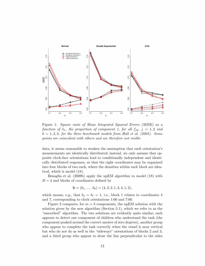
This simulation study compares the nonparametric “EM-like” algorithmfrom Benaglia et al. (2009b), which we refer to as npEM here, with thenew algorithm using the same examples for which Hall et al. (2005) testedtheir estimation technique based on inverting the mixture model. The threesimulated models, described below, are trivariate two-component mixtures(m = 2, r = 3) with independent but not identically distributed repeatedmeasures, i.e., bk = k for k = 1, 2, 3. We ran S = 300 replications of n = 500observations each and computed the errors in terms of the square root ofthe Mean Integrated Squared Error (MISE) for the densities, where

MISEjk =1

S

S∑s=1

∫ (f

(s)jk (u)− fjk(u)

)2du, j = 1, 2 and k = 1, 2, 3;

10

and the integral is computed numerically (using an appropriate function

defined in mixtools). Each density f(s)jk is computed using the weighted

kernel density estimate (17) together with the final values of the posteriorprobabilities ptij after convergence of the algorithm.

The first example is a normal model, for which the individual densities fj`are the pdf’s of N (µj`, 1), with component means µ1 = (0, 0, 0) and µ2 =(3, 4, 5). The second example uses double exponential distributions withdensities fj`(t) = exp−|t− µj`|/2, where µ1 = (0, 0, 0) and µ2 = (3, 3, 3).In the third example, the first component has a central t(10) distributionand thus µ1 = (0, 0, 0), whereas the second component’s coordinates arenoncentral t(10) distributions with noncentrality parameters 3, 4, and 5.Thus, the mean of the third component is µ2 = (3, 4, 5)× 1.0837. Note thatboth algorithms assume only the general model of conditional independence,with bk = k for all k.

Since it has already been shown in Benaglia et al. (2009b) that thenpEM dramatically outperforms the inversion method of Hall et al. (2005)for the three test cases, Figure 1 only compares the npEM against the newalgorithm, which is labeled “smoothed” in the figure. This figure shows thatthe two algorithms provide nearly identical efficiency (in terms of MISE) andthat there is no clear winner for the models and the various settings (λ1)considered.

5.3 The water-level experiment

We consider in this section a dataset from an experiment involving n = 405children aged 11 to 16 years subjected to a water-level task as initially de-scribed by Thomas et al. (1993). In this experiment, each child is presentedwith eight rectangular vessels on a sheet of paper, each tilted to one of r = 8clock-hour orientations: in order of presentation to the subjects, these ori-entations are 11, 4, 2, 7, 10, 5, 1, and 8 o’clock. The children’s task wasto draw a line representing the surface of still liquid in the closed, tiltedvessel in each picture. Each such line describes two points of intersectionwith the sides of the vessel; the acute angle, in degrees, formed between thehorizontal and the line passing through these two points was measured foreach response. The sign of each such measurement was taken to be the signof the slope of the line. The water-level dataset is available in the mixtoolspackage (Young et al., 2009; Benaglia et al., 2009c). This dataset has beenanalyzed previously by Hettmansperger and Thomas (2000) and Elmoreet al. (2004), who assume that the r = 8 coordinates are all conditionallyidentically distributed and then bin the data to produce multinomial vectors(these authors call this a “cutpoint” approach).

However, because of the experimental methodology used to collect the

11

0.04

0.06

0.08

0.10

0.12

0.14

Normal

λ1

MISE

0.1 0.2 0.3 0.4

Smoothed Component 1Smoothed Component 2npEM Component 1 npEM Component 2

0.04

0.06

0.08

0.10

0.12

0.14

Double Exponential

λ10.1 0.2 0.3 0.4

0.04

0.06

0.08

0.10

0.12

0.14

t(10)

λ10.1 0.2 0.3 0.4

Figure 1: Square roots of Mean Integrated Squared Errors (MISE) as afunction of λ1, the proportion of component 1, for all fjk, j = 1, 2 andk = 1, 2, 3, for the three benchmark models from Hall et al. (2005). Somepoints are coincident with others and are therefore not visible.

data, it seems reasonable to weaken the assumption that each orientation’smeasurements are identically distributed; instead, we only assume that op-posite clock-face orientations lead to conditionally independent and identi-cally distributed responses, so that the eight coordinates may be organizedinto four blocks of two each, where the densities within each block are iden-tical, which is model (18).

Benaglia et al. (2009b) apply the npEM algorithm to model (18) withB = 4 and blocks of coordinates defined by

b = (b1, . . . , b8) = (4, 3, 2, 1, 3, 4, 1, 2),

which means, e.g., that b4 = b7 = 1, i.e., block 1 relates to coordinates 4and 7, corresponding to clock orientations 1:00 and 7:00.

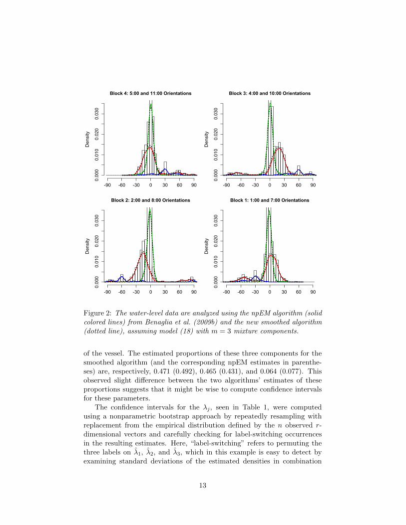
Figure 2 compares, for m = 3 components, the npEM solution with thesolution given by the new algorithm (Section 5.1), which we refer to as the“smoothed” algorithm. The two solutions are evidently quite similar; eachappears to detect one component of children who understand the task (thecomponent peaked around the correct answer of zero degrees), another groupwho appear to complete the task correctly when the vessel is near verticalbut who do not do as well in the “sideways” orientations of blocks 2 and 3,and a third group who appear to draw the line perpendicular to the sides

12

Density

0.000

0.010

0.020

0.030

Block 4: 5:00 and 11:00 Orientations

-90 -60 -30 0 30 60 90

Density

0.000

0.010

0.020

0.030

Block 3: 4:00 and 10:00 Orientations

-90 -60 -30 0 30 60 90

Density

0.000

0.010

0.020

0.030

Block 2: 2:00 and 8:00 Orientations

-90 -60 -30 0 30 60 90

Density

0.000

0.010

0.020

0.030

Block 1: 1:00 and 7:00 Orientations

-90 -60 -30 0 30 60 90

Figure 2: The water-level data are analyzed using the npEM algorithm (solidcolored lines) from Benaglia et al. (2009b) and the new smoothed algorithm(dotted line), assuming model (18) with m = 3 mixture components.

of the vessel. The estimated proportions of these three components for thesmoothed algorithm (and the corresponding npEM estimates in parenthe-ses) are, respectively, 0.471 (0.492), 0.465 (0.431), and 0.064 (0.077). Thisobserved slight difference between the two algorithms’ estimates of theseproportions suggests that it might be wise to compute confidence intervalsfor these parameters.

The confidence intervals for the λj , seen in Table 1, were computedusing a nonparametric bootstrap approach by repeatedly resampling withreplacement from the empirical distribution defined by the n observed r-dimensional vectors and carefully checking for label-switching occurrencesin the resulting estimates. Here, “label-switching” refers to permuting thethree labels on λ1, λ2, and λ3, which in this example is easy to detect byexamining standard deviations of the estimated densities in combination

13

λ1 λ2 λ3

npEM 0.446 0.552 0.337 0.469 0.0542 0.1506Smoothed 0.420 0.527 0.361 0.496 0.0515 0.1594

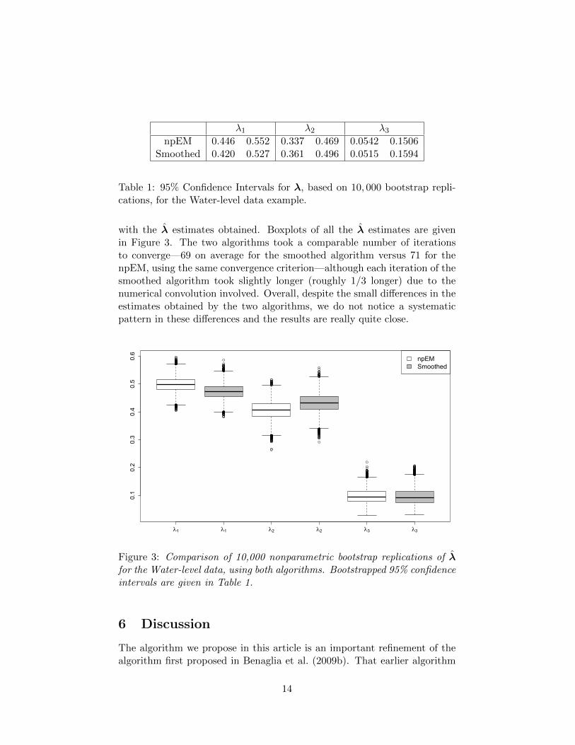
Table 1: 95% Confidence Intervals for λ, based on 10, 000 bootstrap repli-cations, for the Water-level data example.

with the λ estimates obtained. Boxplots of all the λ estimates are givenin Figure 3. The two algorithms took a comparable number of iterationsto converge—69 on average for the smoothed algorithm versus 71 for thenpEM, using the same convergence criterion—although each iteration of thesmoothed algorithm took slightly longer (roughly 1/3 longer) due to thenumerical convolution involved. Overall, despite the small differences in theestimates obtained by the two algorithms, we do not notice a systematicpattern in these differences and the results are really quite close.

λ1 λ1 λ2 λ2 λ3 λ3

0.1

0.2

0.3

0.4

0.5

0.6

npEMSmoothed

Figure 3: Comparison of 10,000 nonparametric bootstrap replications of λfor the Water-level data, using both algorithms. Bootstrapped 95% confidenceintervals are given in Table 1.

6 Discussion

The algorithm we propose in this article is an important refinement of thealgorithm first proposed in Benaglia et al. (2009b). That earlier algorithm

14

is, to the best of our knowledge, the first algorithm that can deal easily withModel (2) in its full generality. It also renders itself to fairly easy coding andproduces error rates that are considerably lower than those of the inversionmethod (easily applicable only when m = 2) of Hall et al. (2005) for a set ofstandard test cases. However, it does not appear to minimize any particularobjective function and therefore cannot be viewed as a true EM algorithm.The new algorithm introduced in this article has a provable descent propertywith respect to a loglikelihood-like quantity. That quantity is, essentially,a penalized Kullback-Leibler distance between the true target density andthe iteratively reweighted sum of smoothed estimated component densities.

We obtain our new algorithm by combining the so-called regularizationapproach with the earlier algorithm of Benaglia et al. (2009b). This ap-proach was used by Eggermont and LaRiccia (1995) and Eggermont (1999)in the context of indirect measurements, where it was applied to an earlierEMS (Smoothed EM) algorithm of Silverman et al. (1990) that does nothave an easy interpretation. The result of the regularization approach thereis a new algorithm, closely related to EMS, called NEMS (Nonlinear EMS).That algorithm has empirical performance almost identical to that of EMS;however, it is a true EM algorithm. In the mixture-model setting, additionalcomputational tools based on a majorization-minimization (MM) theory arenecessary in order to produce an algorithm with a descent property.

The MM device used in our algorithm, namely, the convexity of the neg-ative logarithm in the proof of Lemma 1, is exactly the same as used bya classical EM algorithm. However, the question of whether our algorithmrepresents a true EM algorithm—i.e., whether the right side of Equation (9)is actually the expectation of a loglikelihood function for some idea of “com-plete data”—is largely academic; one feature of this article is that it demon-strates in a practical case how a direct MM approach can produce the sametheoretical advantages as an EM approach.

A future practitioner will have a choice of algorithms when estimatingthe nonparametric multivariate finite mixture model of Equation (2). Thealgorithm we propose in the current paper is the wise choice if a descentproperty and the convergence properties associated with it (e.g., see Langeet al., 2000) are needed. On the other hand, our experimental results vali-date the use of the earlier algorithm of Benaglia et al. (2009b) if only goodempirical performance is desired, since the earlier algorithm appears to pro-duce very similar results to the new, theoretically sound one. Note that ournew algorithm is generally the slower of the two since it involves numericalconvolutions.

The basic algorithm presented in this article may be generalized in sev-eral directions. In addition to the blocking structure introduced in Equa-tion (18), one might posit various location and/or scale models that link

15

the component densities while still allowing the overall parametric form ofthe density functions to be unspecified. A thorough discussion of such gen-eralizations is given in Section 4 of Benaglia et al. (2009b), where even aunivariate application of these algorithms to the case in which the den-sity functions are assumed symmetric is given. Another possible topic offuture research is selection of an appropriate bandwidth h. Complicatingthis selection is the fact that, when estimating a mixture model, one doesnot observe individual component densities. At every step of the algorithm,new estimates of these components are computed; thus, bandwidth selectionproblem in this context may be a problem fundamentally different from theregular bandwidth selection for density estimation purposes. This issue isdiscussed at length by Benaglia et al. (2009a), who recommend an iterativebandwidth selection algorithm. It does not appear that generalization ofour algorithm in any of these many directions would present any seriousdifficulties. Finally, there is the question of asymptotic convergence rates.Empirical studies in Benaglia et al. (2009b) are suggestive of rates of con-vergence of the original npEM algorithm, though no theoretical result onthis subject is yet known. Now that we have demonstrated that our newalgorithm may be used to optimize a particular objective function, it willperhaps be possible to establish such results in the future.

Appendix 1: Some convergence properties

Suppose we fix λ0 and consider the function defined by Equation (13) thatmaps (f0,λ0) 7→ (f ,λ0). Iteratively applying this function yields a sequence

(f0,λ0), (f1,λ0), (f2,λ0), . . . . (20)

Here, we present a few simple convergence results regarding this sequence.The results of this section have analogues in Section 3 of Eggermont (1999)for a slightly different case.

Throughout this section, we will assume for the sake of simplicity thatthe kernel K(·) is strictly positive on the whole real line. We define thesubset B ⊂ F by

B =

Sφ : 0 ≤ φ ∈ F and

∫Ωφj(x) dx = 1 for all j

. (21)

The idea of defining B in this way is that B will contain the whole sequencef0, f1, f2, . . . except possibly the initial f0, where each element in the se-quence is defined by applying equation (13) to the preceding element. Toverify this claim, we simply note that equation (13) may be rewritten as

fjk(u) = Sφ0jk(u), (22)

16

where

φ0jk(xk)

def= αjk

∫· · ·∫g(x)w0

j (x) dx1 · · · dxk−1dxk+1 · · · dxr (23)

must integrate to one because of the definition of αjk. Furthermore, thefunctional f 7→ `(f ,λ) is defined on B because for any (f1, . . . , fm) ∈ B,fj is bounded below by infx∈ΩKh(x) > 0 since we have assumed that theoriginal kernel K(·) is positive; thus, N f is well-defined for f ∈ B.

Lemma 3. The set B is convex and the functional `(f ,λ) of Equation (4)is strictly convex on B for fixed λ.

Proof: Let f1 and f2 be arbitrary elements of B, and take some α ∈(0, 1). The linearity of the S operator implies that αf1 + (1 − α)f2 ∈ B,which establishes the convexity of B immediately.

Furthermore,

`[αf1 + (1− α)f2

]=

∫g(x) log g(x) dx

−∫g(x) log

m∑j=1

λjN[αf1

j + (1− α)f2j

](x) dx.

Focusing on the rightmost term above, we first claim that

N[αf1

j + (1− α)f2j

](x) > αN f1(x) + (1− α)N f2(x)

by the strict concavity of the N operator [Lemma 3.1(iii) of Eggermont(1999)]. Furthermore, the fact that the logarithm function is concave andstrictly increasing implies that

`[αf1 + (1− α)f2,λ

]<

∫g(x) log g(x) dx− α

∫g(x) log

m∑j=1

λjN f1j (x) dx

−(1− α)

∫g(x) log

m∑j=1

λjN f2j (x) dx

= α`(f1,λ) + (1− α)`(f2,λ).

Remark: We may also, using nearly the same proof as for Lemma 3,show that `(f ,λ) is strictly convex in λ for fixed f , though this fact ap-pears less useful. It is not possible to prove that `(f ,λ) is somehow strictlyconvex in the vector (f ,λ) jointly—even if we were to define this conceptrigorously—since we know that, as in all mixture model settings, permutingthe subscripts 1, . . . ,m on (f1, λ1), . . . , (fm, λm) does not change the value

17

of `(f ,λ), which implies that there cannot in general exist a unique globalminimizer of `(f ,λ).

The following lemma establishes a sufficient condition so that the se-quence of functions in (20) is guaranteed to have a uniformly convergentsubsequence. It turns out that, along with the assumptions made earlier,the only additional assumption we will make is that the kernel density func-tion satisfies a Lipschitz continuity condition:

Lemma 4. If there exists L > 0 such that |Kh(x)−Kh(y)| ≤ L|x− y| forany x,y ∈ Ω, then every functional sequence f1, f2, . . . defined by (20) hasa uniformly convergent subsequence.

Proof: Since Ω is a compact subset of Rr, we may assume that thereexist positive constants a < A such that a ≤ Kh(·) ≤ A on Ω. Thus,in Equations (22) and (23), we must have a ≤ fjk ≤ A for all j, k. Weconclude that the sequence |f1|, |f2|, . . . is uniformly bounded.

Furthermore, for arbitrary x,y ∈ Ω and f ∈ B,

|fj(x)− fj(y)| = |Sφj(x)− Sφj(y)|

≤∫|Kh(x− u)−Kh(y − u)||φj(u)| du

≤ L|x− y|

for all j. We conclude that the sequence f1, f2, . . . is uniformly boundedand equicontinuous, so the Arzela-Ascoli Theorem implies that there is auniformly convergent subsequence.

Lemma 5. The functional f 7→ `(f ,λ) is lower semicontinuous on B.

Proof: Consider a sequence of functions fn = (f1,1, . . . , fm,n)′ ∈ B.Let us denote ψ = ψ1, . . . , ψm

′= lim infn fn. By Lemma 4, there always

exists a subsequence fnk→ ψ; without loss of generality, assume that this

subsequence coincides with the entire sequence fn. Since every componentfunction fj,n ∈ B is bounded away from zero then so is the limit functionψ; therefore, log fj,n → logψ. Consequently, N fj,n → Nψj and MλN fn →MλNψ. Since the function ρ(t) = t − log t − 1 ≥ 0, by Fatou’s lemma wehave ∫

g(x)ρ(MλNψ(x)) dx ≤ lim inf

∫g(x)ρ(MλN fn(x)) dx.

From the above, the statement of the proposition follows immediately.Notice that the functional f 7→ `(f ,λ) is uniformly bounded from below

on B, which follows from Equation (6) and the fact that N fj(x) ≤ Sfj(x) =1 by the arithmetic-geometric mean inequality. Thus, the lower semincon-tinuity combined with strict convexity, as proved above, imply that for any

18

fixed λ, the sequence (20) converges to a global maximizer of the functionalf 7→ `(f ,λ). As a practical matter, this means that we could essentiallyreplace `(f ,λ) by the profile loglikelihood

`∗(λ)def= inf

f∈B`(f ,λ)

because the minimization on the right-hand side may be accomplished byiterating (13) until convergence. However, dealing with the profile loglikeli-hood is not the general optimization strategy adopted in Section 4.

References

Allman, E. S., Matias, C., and Rhodes, J. A. (2009). Identifiability ofparameters in latent structure models with many observed variables. Ann.Statist, 37(6A):3099–3132.

Benaglia, T., Chauveau, D., and Hunter, D. R. (2009a). Bandwidth se-lection in an EM-like algorithm for nonparametric multivariate mixtures.Technical Report hal-00353297, hal.

Benaglia, T., Chauveau, D., and Hunter, D. R. (2009b). An EM-like algo-rithm for semi-and non-parametric estimation in multivariate mixtures.Journal of Computational and Graphical Statistics, 18(2):505–526.

Benaglia, T., Chauveau, D., Hunter, D. R., and Young, D. (2009c). mixtools:An R package for analyzing finite mixture models. Journal of StatisticalSoftware, 32(6):1–29.

Dempster, A. P., Laird, N. M., and Rubin, D. B. (1977). Maximum likeli-hood from incomplete data via the em algorithm. Journal of the RoyalStatistical Society, Series B, 39(1):1–38.

Eggermont, P. P. B. (1992). Nonlinear smoothing and the EM algorithm forpositive integral equations of the first kind. Unpublished manuscript.

Eggermont, P. P. B. (1999). Nonlinear smoothing and the em algorithmfor positive integral equations of the first kind. Applied Mathematics andOptimization, 39(1):75–91.

Eggermont, P. P. B. and LaRiccia, V. N. (1995). Maximum smoothed densityestimation for inverse problems. The Annals of Statistics, 23(1):199–220.

Elmore, R. T., Hettmansperger, T. P., and Thomas, H. (2004). Estimatingcomponent cumulative distribution functions in finite mixture models.Comm. Statist. Theory Methods, 33(9):2075–2086.

19

Hall, P., Neeman, A., Pakyari, R., and Elmore, R. T. (2005). Nonparametricinference in multivariate mixtures. Biometrika, 92(3):667–678.

Hall, P. and Zhou, X. H. (2003). Nonparametric estimation of componentdistributions in a multivariate mixture. Annals of Statistics, 31:201–224.

Hettmansperger, T. P. and Thomas, H. (2000). Almost nonparametric in-ference for repeated measures in mixture models. Journal of the RoyalStatistical Society, Series B, 62(4):811–825.

Hunter, D. R. and Lange, K. (2004). A tutorial on MM algorithms. TheAmerican Statistician, 58:30–37.

Kasahara, H. and Shimotsu, K. (2008). Nonparametric identification of finitemixture models of dynamic discrete choices. Econometrica, 77(1):135–176.

Kruskal, J. B. (1977). Three-way arrays: Rank and uniqueness of trilineardecompositions, with application to arithmetic complexity and statistics.Linear algebra and its applications, 18(2):95–138.

Lange, K., Hunter, D. R., and Yang, I. (2000). Optimization transfer usingsurrogate objective functions. Journal of Computational and GraphicalStatistics, 9(1):1–20.

Lindsay, B. G. (1995). Mixture Models: Theory, Geometry, and Applica-tions. Institute of Mathematical Statistics.

R Development Core Team (2008). R: A Language and Environment forStatistical Computing. R Foundation for Statistical Computing, Vienna,Austria. ISBN 3-900051-07-0.

Shepp, L. A. and Vardi, Y. (1982). Maximum likelihood reconstruction foremission tomography. IEEE Trans. Med. Imaging, 1(2):113–122.

Silverman, B. W. (1982). On the estimation of a probability density functionby the maximum penalized likelihood method. The Annals of Statistics,pages 795–810.

Silverman, B. W., Jones, M. C., Wilson, J. D., and Nychka, D. W. (1990). Asmoothed EM algorithm approach to indirect estimation problems, withparticular reference to stereology and emission tomography. Journal ofthe Royal Statistical Society, Series B, 52:271–324.

Thomas, H., Lohaus, A., and Brainerd, C. J. (1993). Modeling growthand individual differences in spatial tasks. Monographs of the Society forResearch in Child Development, 58(9).

20

Vardi, Y., Shepp, L. A., and Kaufman, L. (1985). A statistical model forpositron emission tomography. Journal of the American Statistical Asso-ciation, 80(389):8–20.

Young, D. S., Benaglia, T., Chauveau, D., Elmore, R. T., Hettmansperger,T. P., Hunter, D. R., Thomas, H., and Xuan, F. (2009). mixtools: Toolsfor mixture models. R package version 0.3.3.

21