smoothed analysis of algorithms - arxiv · smoothed analysis of algorithms: ... terpolates between...
TRANSCRIPT

arX
iv:c
s/01
1105
0v7
[cs
.DS]
9 O
ct 2
003
Smoothed Analysis of Algorithms:
Why the Simplex Algorithm Usually Takes Polynomial Time ∗
Daniel A. Spielman †
Department of Mathematics
Massachusetts Institute of Technology
Shang-Hua Teng ‡
Department of Computer Science
Boston University, and
Akamai Technologies Inc.
February 1, 2008
Abstract
We introduce the smoothed analysis of algorithms, which continuously in-terpolates between the worst-case and average-case analyses of algorithms.In smoothed analysis, we measure the maximum over inputs of the expectedperformance of an algorithm under small random perturbations of that in-put. We measure this performance in terms of both the input size and themagnitude of the perturbations. We show that the simplex algorithm hassmoothed complexity polynomial in the input size and the standard deviationof Gaussian perturbations.
∗An extended abstract of this paper appeared in the Proceedings of the 33rd Annual ACM Symposium
on Theory of Computing, pp. 296-305, 2001.†Partially supported by an Alfred P. Sloan Foundation Fellowship, NSF CAREER award CCR-9701304,
NSF grant CCR-0112487, and a Junior Faculty Research Leave sponsored by the M.I.T. School of Science‡Partially suppoted by an Alfred P. Sloan Foundation Fellowship, and NSF grant CCR: 99-72532. Part
of this work was done while at UIUC and visiting the department of mathematics at M.I.T.
1

Contents
1 Introduction 61.1 Linear Programming and the Simplex Method . . . . . . . . . . . . . . . . . 61.2 Smoothed Analysis of Algorithms and Related Work . . . . . . . . . . . . . 81.3 Our Results . . . . . . . . . . . . . . . . . . . . . . . . . . . . . . . . . . . . 101.4 Intuition Through Condition Numbers . . . . . . . . . . . . . . . . . . . . . 101.5 Discussion . . . . . . . . . . . . . . . . . . . . . . . . . . . . . . . . . . . . . 11
2 Notation and Mathematical Preliminaries 132.1 Geometric Definitions . . . . . . . . . . . . . . . . . . . . . . . . . . . . . . 142.2 Vector and Matrix Norms . . . . . . . . . . . . . . . . . . . . . . . . . . . . 152.3 Probability . . . . . . . . . . . . . . . . . . . . . . . . . . . . . . . . . . . . 162.4 Gaussian Random Vectors . . . . . . . . . . . . . . . . . . . . . . . . . . . . 192.5 Changes of Variables . . . . . . . . . . . . . . . . . . . . . . . . . . . . . . . 25
3 The Shadow Vertex Method 283.1 Formal Description . . . . . . . . . . . . . . . . . . . . . . . . . . . . . . . . 283.2 Polar Description . . . . . . . . . . . . . . . . . . . . . . . . . . . . . . . . . 303.3 Two-Phase Method . . . . . . . . . . . . . . . . . . . . . . . . . . . . . . . . 323.4 Discussion . . . . . . . . . . . . . . . . . . . . . . . . . . . . . . . . . . . . . 37
4 Shadow Size 384.1 Distance . . . . . . . . . . . . . . . . . . . . . . . . . . . . . . . . . . . . . . 454.2 Angle of q to ω . . . . . . . . . . . . . . . . . . . . . . . . . . . . . . . . . . 514.3 Extending the shadow bound . . . . . . . . . . . . . . . . . . . . . . . . . . 54
5 Smoothed Analysis of a Two-Phase Simplex Algorithm 575.1 Many Good Choices . . . . . . . . . . . . . . . . . . . . . . . . . . . . . . . 59
5.1.1 Discussion . . . . . . . . . . . . . . . . . . . . . . . . . . . . . . . . . 665.2 Bounding the shadow of LP ′ . . . . . . . . . . . . . . . . . . . . . . . . . . 675.3 Bounding the shadow of LP+ . . . . . . . . . . . . . . . . . . . . . . . . . . 78
6 Discussion and Open Questions 876.1 Practicality of the analysis . . . . . . . . . . . . . . . . . . . . . . . . . . . . 876.2 Further analysis of the simplex algorithm . . . . . . . . . . . . . . . . . . . 876.3 Degeneracy . . . . . . . . . . . . . . . . . . . . . . . . . . . . . . . . . . . . 886.4 Smoothed Analysis . . . . . . . . . . . . . . . . . . . . . . . . . . . . . . . . 88
7 Acknowledgments 89
2

List of Theorems, Lemmas, Corollaries and Propositions
Theorem 2.5.2 (Blaschke) . . . . . . . . . . . . . . . . . . . . . . . . . . . . . . . . . . . . . . . . . . . . . . . . . . . . 25
Theorem 4.0.1 (Shadow Size) . . . . . . . . . . . . . . . . . . . . . . . . . . . . . . . . . . . . . . . . . . . . . . . . 38
Theorem 5.0.1 (Main) . . . . . . . . . . . . . . . . . . . . . . . . . . . . . . . . . . . . . . . . . . . . . . . . . . . . . . . 57
Lemma 2.3.3 (Comparing expectations) . . . . . . . . . . . . . . . . . . . . . . . . . . . . . . . . . . . . . . 16
Lemma 2.3.4 (Similar distributions). . . . . . . . . . . . . . . . . . . . . . . . . . . . . . . . . . . . . . . . . .17
Lemma 2.3.5 (Combination lemma) . . . . . . . . . . . . . . . . . . . . . . . . . . . . . . . . . . . . . . . . . . 17
Lemma 2.3.6 (Generalized combination lemma) . . . . . . . . . . . . . . . . . . . . . . . . . . . . . . 18
Lemma 2.3.7 (Almost polynomial densities) . . . . . . . . . . . . . . . . . . . . . . . . . . . . . . . . . . 18
Lemma 2.4.2 (Smoothness of Gaussians) . . . . . . . . . . . . . . . . . . . . . . . . . . . . . . . . . . . . . 20
Lemma 2.4.11 (Comparing Gaussian tails) . . . . . . . . . . . . . . . . . . . . . . . . . . . . . . . . . . . 23
Lemma 3.3.5 (Shadow path of LP+). . . . . . . . . . . . . . . . . . . . . . . . . . . . . . . . . . . . . . . . . .37
Lemma 4.0.6 (Discretization in limit) . . . . . . . . . . . . . . . . . . . . . . . . . . . . . . . . . . . . . . . . 40
Lemma 4.0.7 (Angle bound) . . . . . . . . . . . . . . . . . . . . . . . . . . . . . . . . . . . . . . . . . . . . . . . . . 41
Lemma 4.0.11 (Angle bound given optSimp) . . . . . . . . . . . . . . . . . . . . . . . . . . . . . . . . . 43
Lemma 4.0.12 (Division into distance and angle) . . . . . . . . . . . . . . . . . . . . . . . . . . . . . 44
Lemma 4.1.1 (Distance bound) . . . . . . . . . . . . . . . . . . . . . . . . . . . . . . . . . . . . . . . . . . . . . . 46
Lemma 4.1.2 (Distance bound in plane) . . . . . . . . . . . . . . . . . . . . . . . . . . . . . . . . . . . . . .46
Lemma 4.1.3 (Height of simplex) . . . . . . . . . . . . . . . . . . . . . . . . . . . . . . . . . . . . . . . . . . . . 49
Lemma 4.2.1 (Angle of incidence) . . . . . . . . . . . . . . . . . . . . . . . . . . . . . . . . . . . . . . . . . . . .51
Lemma 4.2.2 (Angle of incidence, II) . . . . . . . . . . . . . . . . . . . . . . . . . . . . . . . . . . . . . . . . 52
Lemma 4.2.3 (Points under plane) . . . . . . . . . . . . . . . . . . . . . . . . . . . . . . . . . . . . . . . . . . . 53
Lemma 5.1.1 (Many good choices) . . . . . . . . . . . . . . . . . . . . . . . . . . . . . . . . . . . . . . . . . . . 59
Lemma 5.1.6 (Probability of Y jK) . . . . . . . . . . . . . . . . . . . . . . . . . . . . . . . . . . . . . . . . . . . . . 62
Lemma 5.1.7 (Sum over j of Y jK) . . . . . . . . . . . . . . . . . . . . . . . . . . . . . . . . . . . . . . . . . . . . . 62
Lemma 5.1.8 (Sum over K and j of Y jK) . . . . . . . . . . . . . . . . . . . . . . . . . . . . . . . . . . . . . . 62
Lemma 5.1.9 (Relating Xs to Y s) . . . . . . . . . . . . . . . . . . . . . . . . . . . . . . . . . . . . . . . . . . . . 63
Lemma 5.1.10 (Geometric condition for bad I) . . . . . . . . . . . . . . . . . . . . . . . . . . . . . . . 63
Lemma 5.1.11 (Big height, small coefficient) . . . . . . . . . . . . . . . . . . . . . . . . . . . . . . . . . 64
Lemma 5.1.12 (Probability of bad geometry) . . . . . . . . . . . . . . . . . . . . . . . . . . . . . . . . . 65
Lemma 5.2.1 (LP’) . . . . . . . . . . . . . . . . . . . . . . . . . . . . . . . . . . . . . . . . . . . . . . . . . . . . . . . . . . 67
3

Lemma 5.2.2 (probability of small smin
(
AI(A)
)
) . . . . . . . . . . . . . . . . . . . . . . . . . . . . . . 70
Lemma 5.2.3 (From a) . . . . . . . . . . . . . . . . . . . . . . . . . . . . . . . . . . . . . . . . . . . . . . . . . . . . . . .71
Lemma 5.2.4 (Changing α to α) . . . . . . . . . . . . . . . . . . . . . . . . . . . . . . . . . . . . . . . . . . . . . 72
Lemma 5.2.5 (Approximation of α by α) . . . . . . . . . . . . . . . . . . . . . . . . . . . . . . . . . . . . . 73
Lemma 5.2.7 (Proper subset) . . . . . . . . . . . . . . . . . . . . . . . . . . . . . . . . . . . . . . . . . . . . . . . . 74
Lemma 5.2.9 (Jacobian of Ψ) . . . . . . . . . . . . . . . . . . . . . . . . . . . . . . . . . . . . . . . . . . . . . . . . 75
Lemma 5.2.10 (Bound on Jacobian of Ψ) . . . . . . . . . . . . . . . . . . . . . . . . . . . . . . . . . . . . . 75
Lemma 5.2.11 (Jacobian of Γu ,v) . . . . . . . . . . . . . . . . . . . . . . . . . . . . . . . . . . . . . . . . . . . . . 76
Lemma 5.2.12 (Jacobian of Γu ,v in 2D) . . . . . . . . . . . . . . . . . . . . . . . . . . . . . . . . . . . . . . . 77
Lemma 5.3.1 (LP+) . . . . . . . . . . . . . . . . . . . . . . . . . . . . . . . . . . . . . . . . . . . . . . . . . . . . . . . . . 78
Lemma 5.3.2 (LP+ Shadow, part 2) . . . . . . . . . . . . . . . . . . . . . . . . . . . . . . . . . . . . . . . . . . 81
Lemma 5.3.3 (ν) . . . . . . . . . . . . . . . . . . . . . . . . . . . . . . . . . . . . . . . . . . . . . . . . . . . . . . . . . . . . . 82
Lemma 5.3.4 (Almost Gaussian) . . . . . . . . . . . . . . . . . . . . . . . . . . . . . . . . . . . . . . . . . . . . . 83
Lemma 5.3.5 (Almost Gaussian, single variable). . . . . . . . . . . . . . . . . . . . . . . . . . . . . .84
Lemma 5.3.6 (Almost Gaussian, pointwise) . . . . . . . . . . . . . . . . . . . . . . . . . . . . . . . . . . 84
Lemma 5.3.7 (Almost Gaussian, Jacobians) . . . . . . . . . . . . . . . . . . . . . . . . . . . . . . . . . . 85
Corollary 2.4.6 (A chi-square bound) . . . . . . . . . . . . . . . . . . . . . . . . . . . . . . . . . . . . . . . . . 21
Corollary 2.5.3 (Blaschke with s) . . . . . . . . . . . . . . . . . . . . . . . . . . . . . . . . . . . . . . . . . . . . . 26
Corollary 4.3.1 (‖aaa i‖ free) . . . . . . . . . . . . . . . . . . . . . . . . . . . . . . . . . . . . . . . . . . . . . . . . . . . . 55
Corollary 4.3.2 (Gaussians free) . . . . . . . . . . . . . . . . . . . . . . . . . . . . . . . . . . . . . . . . . . . . . . 55
Corollary 4.3.3 (yi free) . . . . . . . . . . . . . . . . . . . . . . . . . . . . . . . . . . . . . . . . . . . . . . . . . . . . . . 56
Corollary 5.1.2 (probability of small smin
(
AI(A)
)
) . . . . . . . . . . . . . . . . . . . . . . . . . . . . . 59
Corollary 5.1.3 (probability of κ in K) . . . . . . . . . . . . . . . . . . . . . . . . . . . . . . . . . . . . . . . . 60
Proposition 2.2.2 (Vectors norms) . . . . . . . . . . . . . . . . . . . . . . . . . . . . . . . . . . . . . . . . . . . . 15
Proposition 2.2.4 (Properties of matrix norm) . . . . . . . . . . . . . . . . . . . . . . . . . . . . . . . . 15
Proposition 2.2.6 (Properties of smin ()) . . . . . . . . . . . . . . . . . . . . . . . . . . . . . . . . . . . . . . . 15
Proposition 2.3.1 (Average ≤ maximum) . . . . . . . . . . . . . . . . . . . . . . . . . . . . . . . . . . . . . 16
Proposition 2.3.2 (Expectation on sub-domain) . . . . . . . . . . . . . . . . . . . . . . . . . . . . . . . 16
Proposition 2.4.1 (Additivity of Gaussians) . . . . . . . . . . . . . . . . . . . . . . . . . . . . . . . . . . . 19
Proposition 2.4.3 (Restrictions of Gaussians) . . . . . . . . . . . . . . . . . . . . . . . . . . . . . . . . . 20
Proposition 2.4.4 (Gaussian measure of halfspaces) . . . . . . . . . . . . . . . . . . . . . . . . . . . 20
4

Proposition 2.4.5 (Chi-Square bound) . . . . . . . . . . . . . . . . . . . . . . . . . . . . . . . . . . . . . . . . 20
Proposition 2.4.7 (Gaussian near point or plane) . . . . . . . . . . . . . . . . . . . . . . . . . . . . . 21
Proposition 2.4.8 (Gamma Inequality) . . . . . . . . . . . . . . . . . . . . . . . . . . . . . . . . . . . . . . . . 22
Proposition 2.4.9 (Non-central Gaussian near the origin) . . . . . . . . . . . . . . . . . . . . . 22
Proposition 2.4.10 (Gaussian tail bound) . . . . . . . . . . . . . . . . . . . . . . . . . . . . . . . . . . . . . 23
Proposition 2.4.12 (Monotonicity of Gaussian density) . . . . . . . . . . . . . . . . . . . . . . . . 24
Proposition 2.5.1 (Change of variables) . . . . . . . . . . . . . . . . . . . . . . . . . . . . . . . . . . . . . . . 25
Proposition 2.5.4 (Latitude and longitude). . . . . . . . . . . . . . . . . . . . . . . . . . . . . . . . . . . .26
Proposition 3.2.2 (Duality) . . . . . . . . . . . . . . . . . . . . . . . . . . . . . . . . . . . . . . . . . . . . . . . . . . . 31
Proposition 3.2.3 (Detecting unbounded programs) . . . . . . . . . . . . . . . . . . . . . . . . . . . 32
Proposition 3.3.1 (Initial simplex of LP ′) . . . . . . . . . . . . . . . . . . . . . . . . . . . . . . . . . . . . . 33
Proposition 3.3.2 (relation of M and κ) . . . . . . . . . . . . . . . . . . . . . . . . . . . . . . . . . . . . . . . 34
Proposition 3.3.3 (Unbounded programs) . . . . . . . . . . . . . . . . . . . . . . . . . . . . . . . . . . . . . 35
Proposition 3.3.4 (Bounded programs) . . . . . . . . . . . . . . . . . . . . . . . . . . . . . . . . . . . . . . . 35
Proposition 4.0.5 (Measure of P) . . . . . . . . . . . . . . . . . . . . . . . . . . . . . . . . . . . . . . . . . . . . . 38
Proposition 4.0.9 (P ⊂ P jI ) . . . . . . . . . . . . . . . . . . . . . . . . . . . . . . . . . . . . . . . . . . . . . . . . . . . . 41
Proposition 5.0.2 (trivial shadow bounds) . . . . . . . . . . . . . . . . . . . . . . . . . . . . . . . . . . . . 58
Proposition 5.1.4 (size of K) . . . . . . . . . . . . . . . . . . . . . . . . . . . . . . . . . . . . . . . . . . . . . . . . . . 61
Proposition 5.2.6 (Volume dilation). . . . . . . . . . . . . . . . . . . . . . . . . . . . . . . . . . . . . . . . . . .74
5

1 Introduction
The Analysis of Algorithms community has been challenged by the existence of remarkablealgorithms that are known by scientists and engineers to work well in practice, but whosetheoretical analyses are negative or inconclusive. The root of this problem is that algorithmsare usually analyzed in one of two ways: by worst-case or average-case analysis. Worst-case analysis can improperly suggest that an algorithm will perform poorly by examining itsperformance under the most contrived circumstances. Average-case analysis was introducedto provide a less pessimistic measure of the performance of algorithms, and many practicalalgorithms perform well on the random inputs considered in average-case analysis. However,average-case analysis may be unconvincing as the inputs encountered in many applicationdomains may bear little resemblance to the random inputs that dominate the analysis.
We propose an analysis that we call smoothed analysis which can help explain the successof algorithms that have poor worst-case complexity and whose inputs look sufficiently dif-ferent from random that average-case analysis cannot be convincingly applied. In smoothedanalysis, we measure the performance of an algorithm under slight random perturbations ofarbitrary inputs. In particular, we consider Gaussian perturbations of inputs to algorithmsthat take real inputs, and we measure the running times of algorithms in terms of theirinput size and the standard deviation of the Gaussian perturbations.
We show that the simplex method has polynomial smoothed complexity. The simplexmethod is the classic example of an algorithm that is known to perform well in practice butwhich takes exponential time in the worst case [KM72, Mur80, GS79, Gol83, AC78, Jer73,AZ99]. In the late 1970’s and early 1980’s the simplex method was shown to converge inexpected polynomial time on various distributions of random inputs by researchers includingBorgwardt, Smale, Haimovich, Adler, Karp, Shamir, Megiddo, and Todd [Bor80, Bor77,Sma83, Hai83, AKS87, AM85, Tod86]. These works introduced novel probabilistic toolsto the analysis of algorithms, and provided some intuition as to why the simplex methodruns so quickly. However, these analyses are dominated by “random looking” inputs: evenif one were to prove very strong bounds on the higher moments of the distributions ofrunning times on random inputs, one could not prove that an algorithm performs well inany particular small neighborhood of inputs.
To bound expected running times on small neighborhoods of inputs, we consider linearprogramming problems in the form
maximize z Tx
subject to Ax ≤ y , (1)
and prove that for every vector z and every matrix A and vector y , the expectation overstandard deviation σ (maxi ‖(yi, a i)‖) Gaussian perturbations A and y of A and y of thetime taken by a two-phase shadow-vertex simplex method to solve such a linear program ispolynomial in 1/σ and the dimensions of A.
1.1 Linear Programming and the Simplex Method
It is difficult to overstate the importance of linear programming to optimization. Linearprogramming problems arise in innumerable industrial contexts. Moreover, linear program-
6

ming is often used as a fundamental step in other optimization algorithms. In a linearprogramming problem, one is asked to maximize or minimize a linear function over a poly-hedral region.
Perhaps one reason we see so many linear programs is that we can solve them efficiently.In 1947, Dantzig [Dan51] introduced the simplex method, which was the first practical ap-proach to solving linear programs and which remains widely used today. To state it roughly,the simplex method proceeds by walking from one vertex to another of the polyhedron de-fined by the inequalities in (1). At each step, it walks to a vertex that is better with respectto the objective function. The algorithm will either determine that the constraints areunsatisfiable, determine that the objective function is unbounded, or reach a vertex fromwhich it cannot make progress, which necessarily optimizes the objective function.
Because of its great importance, other algorithms for linear programming have beeninvented. In 1979, Khachiyan [Kha79] applied the ellipsoid algorithm to linear programmingand proved that it always converged in time polynomial in d, n, and L—the number of bitsneeded to represent the linear program. However, the ellipsoid algorithm has not beencompetitive with the simplex method in practice. In contrast, the interior-point methodintroduced in 1984 by Karmarkar [Kar84], which also runs in time polynomial in d, n, andL, has performed very well: variations of the interior point method are competitive withand occasionally superior to the simplex method in practice.
In spite of half a century of attempts to unseat it, the simplex method remains the mostpopular method for solving linear programs. However, there has been no satisfactory the-oretical explanation of its excellent performance. A fascinating approach to understandingthe performance of the simplex method has been the attempt to prove that there alwaysexists a short walk from each vertex to the optimal vertex. The Hirsch conjecture statesthat there should always be a walk of length at most n − d. Significant progress on thisconjecture was made by Kalai and Kleitman [KK92], who proved that there always existsa walk of length at most nlog2 d+2. However, the existence of such a short walk does notimply that the simplex method will find it.
A simplex method is not completely defined until one specifies its pivot rule—the methodby which it decides which vertex to walk to when it has many to choose from. Thereis no deterministic pivot rule under which the simplex method is known to take a sub-exponential number of steps. In fact, for almost every deterministic pivot rule there is afamily of polytopes on which it is known to take an exponential number of steps [KM72,Mur80, GS79, Gol83, AC78, Jer73]. (See [AZ99] for a survey and a unified construction ofthese polytopes). The best present analysis of randomized pivot rules shows that they take
expected time nO(√
d)[Kal92, MSW96], which is quite far from the polynomial complexityobserved in practice. This inconsistency between the exponential worst-case behavior of thesimplex method and its everyday practicality leave us wanting a more reasonable theoreticalanalysis.
Various average-case analyses of the simplex method have been performed. Most rele-vant to this paper is the analysis of Borgwardt [Bor77, Bor80], who proved that the simplexmethod with the shadow vertex pivot rule runs in expected polynomial time for polytopeswhose constraints are drawn independently from spherically symmetric distributions (e.g.Gaussian distributions centered at the origin). Independently, Smale [Sma83, Sma82] provedbounds on the expected running time of Lemke’s self-dual parametric simplex algorithm on
7

linear programming problems chosen from a spherically-symmetric distribution. Smale’sanalysis was substantially improved by Megiddo [Meg86].
While these average-case analyses are significant accomplishments, it is not clear whetherthey actually provide intuition for what happens on typical inputs. Edelman [Ede92] writeson this point:
What is a mistake is to psychologically link a random matrix with the intu-itive notion of a “typical” matrix or the vague concept of “any old matrix.”
Another model of random linear programs was studied in a line of research initiatedindependently by Haimovich [Hai83] and Adler [Adl83]. Their works considered the maxi-mum over matrices, A, of the expected time taken by parametric simplex methods to solvelinear programs over these matrices in which the directions of the inequalities are chosen atrandom. As this framework considers the maximum of an average, it may be viewed as aprecursor to smoothed analysis—the distinction being that the random choice of inequali-ties cannot be viewed as a perturbation, as different choices yield radically different linearprograms. Haimovich and Adler both proved that parametric simplex methods would takean expected linear number of steps to go from the vertex minimizing the objective functionto the vertex maximizing the objective function, even conditioned on the program beingfeasible. While their theorems confirmed the intuitions of many practitioners, they weregeometric rather than algorithmic1 as it was not clear how an algorithm would locate eithervertex. Building on these analyses, Todd [Tod86], Adler and Megiddo [AM85], and Adler,Karp and Shamir [AKS87] analyzed parametric algorithms for linear programming underthis model and proved quadratic bounds on their expected running time. While the randominputs considered in these analyses are not as special as the random inputs obtained fromspherically symmetric distributions, the model of randomly flipped inequalities provokessome similar objections.
1.2 Smoothed Analysis of Algorithms and Related Work
We introduce the smoothed analysis of algorithms in the hope that it will help explain thegood practical performance of many algorithms that worst-case does not and for whichaverage-case analysis is unconvincing. Our first application of the smoothed analysis ofalgorithms will be to the simplex method. We will consider the maximum over A and y ofthe expected running time of the simplex method on inputs of the form
maximize z Tx
subject to (A + G)x ≤ (y + h), (2)
where we let A and y be arbitrary and G and h be a matrix and a vector of independentlychosen Gaussian random variables of mean 0 and standard deviation σ (maxi ‖(yi, a i)‖). Ifwe let σ go to 0, then we obtain the worst-case complexity of the simplex method; whereas,if we let σ be so large that G swamps out A, we obtain the average-case analyzed byBorgwardt. By choosing polynomially small σ, this analysis combines advantages of worst-case and average-case analysis, and roughly corresponds to the notion of imprecision inlow-order digits.
1Our results in Section 4 are analogous to these results.
8

In a smoothed analysis of an algorithm, we assume that the inputs to the algorithm aresubject to slight random perturbations, and we measure the complexity of the algorithm interms of the input size and the standard deviation of the perturbations. If an algorithm haslow smoothed complexity, then one should expect it to work well in practice since most real-world problems are generated from data that is inherently noisy. Another way of thinkingabout smoothed complexity is to observe that if an algorithm has low smoothed complexity,then one must be unlucky to choose an input instance on which it performs poorly.
We now provide some definitions for the smoothed analysis of algorithms that take realor complex inputs. For an algorithm A and input x , let
CA(x )
be a complexity measure of A on input x . Let X be the domain of inputs to A, and letXn be the set of inputs of size n. The size of an input can be measured in various ways.Standard measures are the number of real variables contained in the input and the sumsof the bit-lengths of the variables. Using this notation, one can say that A has worst-caseC-complexity f(n) if
maxx∈Xn
(CA(x )) = f(n).
Given a family of distributions µn on Xn, we say that A has average-case C-complexity f(n)under µ if
Ex
µn←Xn
[CA(x )] = f(n).
Similarly, we say that A has smoothed C-complexity f(n, σ) if
maxx∈Xn
Eg
[CA(x + (σ ‖x‖?) g)] = f(n, σ), (3)
where (σ ‖x‖?) g is a vector of Gaussian random variables of mean 0 and standard deviationσ ‖x‖? and ‖x‖? is a measure of the magnitude of x , such as the largest element or the norm.We say that an algorithm has polynomial smoothed complexity if its smoothed complexity ispolynomial in n and 1/σ. In Section 6, we present some generalizations of the definition ofsmoothed complexity that might prove useful. To further contrast smoothed analysis withaverage-case analysis, we note that the probability mass in (3) is concentrated in a region ofradius O(σ
√n) and volume at most O(σ
√n)n, and so, when σ is small, this region contains
an exponentially small fraction of the probability mass in an average-case analysis. Thus,even an extension of average-case analysis to higher moments will not imply meaningfulbounds on smoothed complexity.
A discrete analog of smoothed analysis has been studied in a collection of works inspiredby Santha and Vazirani’s semi-random source model [SV86]. In this model, an adversarygenerates an input, and each bit of this input has some probability of being flipped. Blumand Spencer [BS95] design a polynomial-time algorithm that k-colors k-colorable graphsgenerated by this model. Feige and Krauthgamer [FK] analyze a model in which the adver-sary is more powerful, and use it to show that Turner’s algorithm [Tur86] for approximatingthe bandwidth performs well on semi-random inputs. They also improve Turner’s analysis.Feige and Kilian [FK98] present polynomial-time algorithms that recover large independentsets, k-colorings, and optimal bisections in semi-random graphs. They also demonstratethat significantly better results would lead to surprising collapses of complexity classes.
9

1.3 Our Results
We consider the maximum over z , y , and a1, . . . , an of the expected time taken by a two-phase shadow vertex simplex method to solve linear programming problems of the form
maximize z Tx
subject to 〈aaa i|x 〉 ≤ yi, for 1 ≤ i ≤ n, (4)
where each aaai is a Gaussian random vector of standard deviation σ maxi ‖(yi, a i)‖ centeredat a i, and each yi is a Gaussian random variable of standard deviation σ maxi ‖(yi, a i)‖centered at yi.
We begin by considering the case in which y = 1, ‖a i‖ ≤ 1, and σ < 1/3√
d ln n. Inthis case, our first result, Theorem 4.0.1, says that for every vector t the expected size ofthe shadow of the polytope—the projection of the polytope defined by the equations (4)onto the plane spanned by t and z—is polynomial in n, the dimension, and 1/σ. Thisresult is the geometric foundation of our work, but it does not directly bound the runningtime of an algorithm, as the shadow relevant to the analysis of an algorithm depends onthe perturbed program and cannot be specified beforehand as the vector t must be. InSection 3.3, we describe a two-phase shadow-vertex simplex algorithm, and in Section 5 weuse Theorem 4.0.1 as a black box to show that it takes expected time polynomial in n, d,and 1/σ in the case described above.
Efforts have been made to analyze how much the solution of a linear program canchange as its data is perturbed. For an introduction to such analyses, and an analysis ofthe complexity of interior point methods in terms of the resulting condition number, werefer the reader to the work of Renegar [Ren95b, Ren95a, Ren94].
1.4 Intuition Through Condition Numbers
For those already familiar with the simplex method and condition numbers, we include thissection to provide some intuition for why our results should be true.
Our analysis will exploit geometric properties of the condition number of a matrix, ratherthan of a linear program. We start with the observation that if a corner of a polytope isspecified by the equation AIx = y I , where I is a d-set, then the condition number of thematrix AI provides a good measure of how far the corner is from being flat. Moreover, it isrelatively easy to show that if A is subject to perturbation, then it is unlikely that AI haspoor condition number. So, it seems intuitive that if A is perturbed, then most corners ofthe polytope should have angles bounded away from being flat. This already provides someintuition as to why the simplex method should run quickly: one should make reasonableprogress as one rounds a corner if it is not too flat.
There are two difficulties in making the above intuition rigorous: the first is that evenif AI is well-conditioned for most sets I, it is not clear that AI will be well-conditioned formost sets I that are bases of corners of the polytope. The second difficulty is that evenif most corners of the polytope have reasonable condition number, it is not clear that asimplex method will actually encounter many of these corners. By analyzing the shadowvertex pivot rule, it is possible to resolve both of these difficulties.
The first advantage of studying the shadow vertex pivot rule is that its analysis comesdown to studying the expected sizes of shadows of the polytope. From the specification of
10

the plane onto which the polytope will be projected, one obtains a characterization of allthe corners that will be in the shadow, thereby avoiding the complication of an iterativecharacterization. The second advantage is that these corners are specified by the propertythat they optimize a particular objective function, and using this property one can actuallybound the probability that they are ill-conditioned. While the results of Section 4 are notstated in these terms, this is the intuition behind them.
Condition numbers also play a fundamental role in our analysis of the shadow-vertexalgorithm. The analysis of the algorithm differs from the mere analysis of the sizes ofshadows in that, in the study of an algorithm, the plane onto which the polytope is pro-jected depends upon the polytope itself. This correlation of the plane with the polytopecomplicates the analysis, but is also resolved through the help of condition numbers. Inour analysis, we view the perturbation as the composition of two perturbations, where thesecond is small relative to the first. We show that our choice of the plane onto which weproject the shadow is well-conditioned with high probability after the first perturbation.That is, we show that the second perturbation is unlikely to substantially change the planeonto which we project, and therefore unlikely to substantially change the shadow. Thus, itsuffices to measure the expected size of the shadow obtained after the second perturbationonto the plane that would have been chosen after just the first perturbation.
The technical lemma that enables this analysis, Lemma 5.1.1, is a concentration resultthat proves that it is highly unlikely that almost all of the minors of a random matrix havepoor condition number. This analysis also enables us to show that it is highly unlikely thatwe will need a large “big-M” in phase I of our algorithm.
We note that the condition numbers of the AIs have been studied before in the complex-ity of linear programming algorithms. The condition number χA of Vavasis and Ye [VY96]measures the condition number of the worst sub-matrix AI , and their algorithm runs intime proportional to ln(χA). Todd, Tuncel, and Ye [TTY01] have shown that for a Gaus-sian random matrix the expectation of ln(χA) is O(min(d ln n, n)). That is, they show thatit is unlikely that any AI is exponentially ill-conditioned. It is relatively simple to applythe techniques of Section 5.1 to obtain a similar result in the smoothed case. We won-der whether our concentration result that it is exponentially unlikely that many AI areeven polynomially ill-conditioned could be used to obtain a better smoothed analysis of theVavasis-Ye algorithm.
1.5 Discussion
One can debate whether the definition of polynomial smoothed complexity should be thatan algorithm have complexity polynomial in 1/σ or log(1/σ). We believe that the choiceof being polynomial in 1/σ will prove more useful as the other definition is too strong andquite similar to the notion of being polynomial in the worst case. In particular, one canconvert any algorithm for linear programming whose smoothed complexity is polynomial ind, n and log(1/σ) into an algorithm whose worst-case complexity is polynomial in d, n, andL. That said, one should certainly prefer complexity bounds that are lower as a function of1/σ, d and n.
We also remark that a simple examination of the constructions that provide exponentiallower bounds for various pivot rules [KM72, Mur80, GS79, Gol83, AC78, Jer73] reveals that
11

none of these pivot rules have smoothed complexity polynomial in n and sub-polynomial in1/σ. That is, these constructions are unaffected by exponentially small perturbations.
12
2 Notation and Mathematical Preliminaries
In this section, we define the notation that will be used in the paper. We will also reviewsome background from mathematics and derive a few simple statements that we will need.The reader should probably skim this section now, and save a more detailed examinationfor when the relevant material is referenced.
• [n] denotes the set of integers between 1 and n, and([n]
k
)
denotes the subsets of [n] ofsize k.
• Subsets of [n] are denoted by the capital Roman letters I, J, L,K. M will denote asubset of integers, and K will denote a set of subsets of [n].
• Subsets of IR? are denoted by the capital Roman letters A,B,P,Q,R, S, T, U, V .
• Vectors in IR? are denoted by bold lower-case Roman letters, such as aaa i, a i, a i, b i, ci,di,h , t , q , z ,y .
• Whenever a vector, say aaa ∈ IRd is present, its components will be denoted by lower-case Roman letters with subscripts, such as a1, . . . , ad.
• Whenever a collection of vectors, such as aaa1, . . . ,aaan, are present, the similar boldupper-case letter, such as A, will denote the matrix of these vectors. For I ∈
([n]k
)
,AI will denote the matrix of those aaai for which i ∈ I.
• Matrices are denoted by bold upper-case Roman letters, such as A, A, A,B ,M andRω.
• Sd−1 denotes the unit sphere in IRd.
• Vectors in S? will be denoted by bold Greek letters, such as ω,ψ, τ .
• Generally speaking, univariate quantities with scale, such as lengths or heights, willbe represented by lower case Roman letters such as c, h, l, r, s, and t. The principalexceptions are that κ and M will also denote such quantities.
• Quantities without scale, such as the ratios of quantities with scale or affine coor-dinates, will be represented by lower case Greek letters such as α, β, λ, ξ, ζ. α willdenote a vector of such quantities such as (α1, . . . , αd).
• Density functions are denoted by lower case Greek letters such as µ and ν.
• The standard deviations of Gaussian random variables are denoted by lower-caseGreek letters such as σ, τ and ρ.
• Indicator random variables are denoted by upper case Roman letters, such as A, B,E, F , V , W , X, Y , and Z
• Functions into the reals or integers will be denoted by calligraphic upper-case letters,such as F ,G,S+,S ′,T .
13

• Functions into IR? are denoted by upper-case Greek letters, such as Φǫ,Υ,Ψ.
• 〈x |y〉 denotes the inner product of vectors x and y .
• For vectors ω and z , we let angle (ω, z ) denote the angle between these vectors atthe origin.
• The logarithm base 2 is written lg and the natural logarithm is written ln.
• The probability of an event A is written Pr [A], and the expectation of a variable Xis written E [X].
• The indicator random variable for an event A is written [A].
2.1 Geometric Definitions
For the following definitions, we let aaa1, . . . ,aaak denote a set of vectors in IRd.
• Span (aaa1, . . . ,aaak) denotes the subspace spanned by aaa1, . . . ,aaak.
• Aff (aaa1, . . . ,aaak) denotes the hyperplane that is the affine span of aaa1, . . . ,aaak: the setof points
∑
i αiaaai, where∑
i αi = 1, for all i.
• ConvHull (aaa1, . . . ,aaak) denotes the convex hull of aaa1, . . . ,aaak.
• Cone (aaa1, . . . ,aaak) denotes the positive cone through aaa1, . . . ,aaak: the set of points∑
i αiaaai, for αi ≥ 0.
• △ (aaa1, . . . ,aaad) denotes the simplex ConvHull (aaa1, . . . ,aaad).
For a linear program specified by aaa1, . . . ,aaan, y and z , we will say that the linear programis in general position if
• The points aaa1, . . . ,aaan are in general position with respect to y , which means that forall I ⊂
([n]d
)
and x = A−1I yI , and all j 6∈ I, 〈aaaj |x 〉 6= yj.
• For all I ⊂( [n]d−1
)
, z 6∈ Cone (AI).
Furthermore, we will say that the linear program is in general position with respect to avector t if the set of λ for which there exists an I ∈
( [n]d−1
)
such that
(1 − λ)t + λz ∈ Cone (AI)
is finite and does not contain 0.
14

2.2 Vector and Matrix Norms
The material of this section is principally used in Sections 3.3 and 5.1. The followingdefinitions and propositions are standard, and may be found in standard texts on NumericalLinear Algebra.
Definition 2.2.1 (Vector Norms) For a vector x , we define
• ‖x‖ =√
∑
i x2i .
• ‖x‖1 =∑
i |xi|.
• ‖x‖∞ = maxi |xi|.
Proposition 2.2.2 (Vectors norms) For a vector x ∈ IRd,
‖x‖ ≤ ‖x‖1 ≤√
d ‖x‖ .
Definition 2.2.3 (Matrix norm) For a matrix A, we define
‖A‖ def= max
x‖Ax‖ / ‖x‖ .
Proposition 2.2.4 (Properties of matrix norm) For d-by-d matrices A and B , and ad-vector x ,
(a) ‖Ax‖ ≤ ‖A‖ ‖x‖.
(b) ‖AB‖ ≤ ‖A‖ ‖B‖.
(c) ‖A‖ =∥
∥AT∥
∥.
(d) ‖A‖ ≤√
dmaxi ‖aaa i‖, where A = (aaa1, . . . ,aaad).
(e) det (A) ≤ ‖A‖d.
Definition 2.2.5 (smin ()) For a matrix A, we define
smin (A)def=∥
∥A−1∥
∥
−1.
We recall that smin (A) is the smallest singular value of the matrix A, and that it is not anorm.
Proposition 2.2.6 (Properties of smin ()) For d-by-d matrices A and B ,
(a) smin (A) = minx ‖Ax‖ / ‖x‖.
(b) smin (B) ≥ smin (A) − ‖A−B‖ .
15
2.3 Probability
For an event, A, we let [A] denote the indicator random variable for the event. We generallydescribe random variables by their density functions. If x has density µ, then
Pr [A(x )]def=
∫
[A(x )] µ(x ) dx .
If B is another event, then
PrB
[A(x )]def= Pr
[
A(x )∣
∣B(x )] def
=
∫
[B(x )] [A(x )]µ(x ) dx∫
[B(x )] µ(x ) dx.
In a context where multiple densities are present, we will use use the notation Prµ [A(x )]to indicate the probability of A when x is distributed according to µ.
In many situations, we will not know the density µ of a random variable x , but rathera function ν such that ν(x ) = cµ(x ) for some constant c. In this case, we will say that x
has density proportional to ν.The following Propositions and Lemmas will play a prominent role in the proofs in this
paper. The only one of these which might not be intuitively obvious is Lemma 2.3.5.
Proposition 2.3.1 (Average ≤ maximum) Let µ(x, y) be a density function, and letx and y be distributed according to µ(x, y). If A(x, y) is an event and X(x, y) is randomvariable, then
Prx,y
[A(x, y)] ≤ maxx
Pry
[A(x, y)] , and
Ex,y
[X(x, y)] ≤ maxx
Ey
[X(x, y)] ,
where in the right-hand terms, y is distributed according to the induced distribution µ(x, y).
Proposition 2.3.2 (Expectation on sub-domain) Let x be a random variable and A(x )an event. Let P be a measurable subset of the domain of x . Then,
Prx∈P
[A(x )] ≤ Pr [A(x )] /Pr [x ∈ P ] .
Proof By the definition of conditional probability,
Prx∈P
[A(x )] = Pr [A(x )|x ∈ P ]
= Pr [A(x ) and x ∈ P ] /Pr [x ∈ P ] , by Bayes’ rule,
≤ Pr [A(x )] /Pr [x ∈ P ] .
Lemma 2.3.3 (Comparing expectations) Let X and Y be non-negative random vari-ables and A an event satisfying (1) X ≤ k, (2) Pr [A] ≥ 1 − ǫ, and (3) there exists aconstant c such that E [X|A] ≤ cE [Y |A]. Then,
E [X] ≤ cE [Y ] + ǫk.
16

Proof
E [X] = E [X|A]Pr [A] + E [X|not(A)]Pr [not(A)]
≤ cE [Y |A]Pr [A] + ǫk
≤ cE [Y ] + ǫk,
by Proposition 2.3.2.
Lemma 2.3.4 (Similar distributions) Let X be a non-negative random variable suchthat X ≤ k. Let ν and µ be density functions for which there exists a set S such that (1)Prν [S] > 1 − ǫ and (2) there exists a constant c ≥ 1 such that for all a ∈ S, ν(a) ≤ cµ(a).Then,
Eν
[X(a)] ≤ cEµ
[X(a)] + kǫ.
Proof We write
Eν
[X] =
∫
a∈SX(a)ν(a) da +
∫
a6∈SX(a)ν(a) da
≤ c
∫
a∈SX(a)µ(a) da + kǫ
≤ c
∫
aX(a)µ(a) da + kǫ
= cEµ
[X] + kǫ.
Lemma 2.3.5 (Combination lemma) Let x and y be random variables distributed ac-cording to µ(x, y). Let F(x) and G(x, y) be non-negative functions and α and β be constantssuch that
• ∀ǫ ≥ 0, Prx,y [F(x) ≤ ǫ] ≤ αǫ, and
• ∀ǫ ≥ 0, maxx Pry [G(x, y) ≤ ǫ] ≤ (βǫ)2,
where in the second line y is distributed according to the induced density µ(x, y). Then
Prx,y
[F(x)G(x, y) ≤ ǫ] ≤ 4αβǫ.
Proof Consider any x and y for which F(x)G(x, y) ≤ ǫ. If i is the integer for which
2iβǫ < F(x) ≤ 2i+1βǫ,
then G(x, y) ≤ 2−i/β. Thus, F(x)G(x, y) ≤ ǫ, implies that either F(x) ≤ 2βǫ, or thereexists an integer i ≥ 1 for which
F(x) ≤ 2i+1βǫ and G(x, y) ≤ 2−i/β.
17

So, we obtain the bound
Prx,y
[F(x)G(x, y) ≤ ǫ] ≤ Prx,y
[F(x) ≤ 2βǫ] +∑
i≥1
Prx,y
[
F(x) ≤ 2i+1βǫ and G(x, y) ≤ 2−i/β]
≤ 2αβǫ +∑
i≥1
Prx,y
[
F(x) ≤ 2i+1βǫ]
Prx,y
[
G(x, y) ≤ 2−i/β∣
∣F(x) ≤ 2i+1βǫ]
≤ 2αβǫ +∑
i≥1
Prx,y
[
F(x) ≤ 2i+1βǫ]
maxx
Pry
[
G(x, y) ≤ 2−i/β]
≤ 2αβǫ +∑
i≥1
(
2i+1αβǫ) (
2−i)2
, by Proposition 2.3.1,
= 2αβǫ + αβǫ∑
i≥1
21−i
= 4αβǫ.
As we have found this lemma very useful in our work, and we suspect others may aswell, we state a more broadly applicable generalization. It’s proof is similar.
Lemma 2.3.6 (Generalized combination lemma) Let x and y be random variablesdistributed according to µ(x, y). There exists a function c(a, b) such that if F(x) and G(x, y)are non-negative functions and α, β, a and b are constants such that
• Prx,y [F(x) ≤ ǫ] ≤ (αǫ)a, and
• maxx Pry [G(x, y) ≤ ǫ] ≤ (βǫ)b,
where in the second line y is distributed according to the induced density µ(x, y), then
Prx,y
[F(x)G(x, y) ≤ ǫ] ≤ c(a, b)αβǫmin(a,b) lg(1/ǫ)[a=b],
where [a = b] is 1 if a = b and 0 otherwise.
Lemma 2.3.7 (Almost polynomial densities) Let k > 0 and let t be a non-negativerandom variable with density proportional to µ(t)tk such that, for some t0 > 0,
max0≤t≤t0 µ(t)
min0≤t≤t0 µ(t)≤ c.
Then,Pr [t < ǫ] < c(ǫ/t0)
k+1.
18

Proof For ǫ ≥ t0, the lemma is vacuously true. Assuming ǫ < t0,
Pr [t < ǫ] ≤ Pr [t < ǫ]
Pr [t < t0]
=
∫ ǫt=0 µ(t)tk dt∫ t0t=0 µ(t)tk dt
≤ max0≤t≤t0 µ(t)∫ ǫt=0 tk dt
min0≤t≤t0 µ(t)∫ t0t=0 tk dt
≤ cǫk+1/(k + 1)
tk+10 /(k + 1)
= c(ǫ/t0)k+1.
2.4 Gaussian Random Vectors
For the convenience of the reader, we recall some standard facts about Gaussian randomvariables and vectors. These may be found in [Fel68, VII.1] and [Fel71, III.6]. We thendraw some corollaries of these facts and derive some lemmas that we will need later in thepaper.
We first recall that a univariate Gaussian distribution with mean 0 and standard devi-ation σ has density
1√2πσ
e−a2/2σ2,
and that a Gaussian random vector in IRd centered at a point a with covariance matrix M
has density1
(√2π)d
det(M )e−(aaa−a)T M−1(aaa−a)/2.
For positive-definite M , there exists a basis in which the density can be written
d∏
i=1
1√2πσi
e−a2i /2σ2
i ,
where σ21 ≤ · · · ≤ σ2
d are the eigenvalues of M . When all the eigenvalues of M are thesame and equal to σ, then we will refer to the density as a Gaussian distribution of standarddeviation σ.
Proposition 2.4.1 (Additivity of Gaussians) If aaa1 is a Gaussian random vector withcovariance matrix M 1 centered at a point a1 and aaa2 is a Gaussian random vector withcovariance matrix M 2 centered at a point a2, then aaa1 + aaa2 is the Gaussian random vectorwith covariance matrix M 1 + M 2 centered at a1 + a2.
19

Lemma 2.4.2 (Smoothness of Gaussians) Let µ(x ) be a Gaussian distribution of stan-dard deviation σ centered at a point aaa. Let k ≥ 1, let dist (x , aaa) ≤ k and let dist (x ,y) <ǫ ≤ k. Then,
µ(y)
µ(x )≥ e−3kǫ/2σ2
.
Proof By translating aaa, x and y , we may assume aaa = 0 and ‖x‖ ≤ k. We then have
µ(y)
µ(x )= e−(‖y‖2−‖x‖2)/2σ2
≥ e−(2ǫ‖x‖+ǫ2)/2σ2, as ‖y‖ ≤ ‖x‖ + ǫ
≥ e−(2ǫk+ǫ2)/2σ2, as ‖x‖ ≤ k
≥ e−3ǫk/2σ2as ǫ ≤ k.
Proposition 2.4.3 (Restrictions of Gaussians) Let µ be a Gaussian distribution of stan-dard deviation σ centered at a point aaa. Let v be any vector and r any real. Then, the induceddistribution
µ(x |vTx = r)
is a Gaussian distribution of standard deviation σ centered at the projection of aaa onto theplane
{
x : vTx = r}
.
Proposition 2.4.4 (Gaussian measure of halfspaces) Let ω be any unit vector in IRd
and r any real. Then,
(
1√2πσ
)d ∫
g
[〈ω|g〉 ≤ r] e−‖g‖2/2σ2
dg =1√2πσ
∫ t=r
t=−∞e−t2/2σ2
dt
Proof Immediate if one expresses the Gaussian density in a basis containing ω.
The distribution of the square of the norm of a Gaussian random vector is the Chi-Square distribution. We use the following weak bound on the Chi-Square distribution,which follows from Equality (26.4.8) of [AS70].
Proposition 2.4.5 (Chi-Square bound) Let x be a Gaussian random vector in IRd ofstandard deviation σ centered at the origin. Then,
Pr [‖x‖ ≥ kσ] ≤(
k2)d/2−1
e−k2/2
2d/2−1Γ(d2)
. (5)
From this, we derive
20

Corollary 2.4.6 (A chi-square bound) Let x be a Gaussian random vector in IRd ofstandard deviation σ centered at the origin. Then, for n ≥ 3
Pr[
‖x‖ ≥ 3√
d ln nσ]
≤ n−2.9d.
Moreover, if n > d ≥ 3, and x 1, . . . ,xn are such vectors, then
Pr
[
maxi
‖x i‖ ≥ 3√
d ln nσ
]
≤ n−2.9d+1 ≤ 0.0015
(
n
d
)−1
.
Proof For α = 3√
ln nσ we can apply Stirling’s formula [AS70] to (5) to find
Pr[
‖x‖ ≥ α√
d]
≤ (α2d)d/2−1e−α2d/2ed/2√
d/2
2d/2−1(d/2)d/2√
2π
=(
α2)d/2−1
e−(α2−1)d/2 dd/2−1√
d
2d/2−1(d/2)d/22√
π
=(
α2)d/2−1
e−(α2−1)d/2 1√dπ
≤(
α2)d/2
e−(α2−1)d/2
= e−(α2−ln(α2)−1)d/2
≤ e−2.9d ln n
= n−2.9d,
as(α2 − ln(α2) − 1) = 9 ln(n) − ln(9 ln n) − 1 ≥ ln(n)(9 − ln 9 − 1) ≥ 5.8 ln(n).
We also prove it is unlikely that a Gaussian random variable has small norm.
Proposition 2.4.7 (Gaussian near point or plane) Let x be a d-dimensional Gaus-sian random vector of standard deviation σ centered anywhere. Then,
(a) For any point p, Pr [dist (x ,p) ≤ ǫ] ≤(
min(
1,√
e/d)
(ǫ/σ))d
, and
(b) For a plane H of dimension h, Pr [dist (x ,H) ≤ ǫ] ≤ (ǫ/σ)d−h.
Proof Let x be the center of the Gaussian distribution, and let Bǫ(p) denote the ball ofradius ǫ around p. Recall that the volume of Bǫ(p) is
2πd/2ǫd
dΓ(d/2).
To prove part (a), we bound the probability that dist (x ,p) ≤ ǫ by
(
1√2πσ
)d ∫
x∈Bǫ(p)e−‖(x−x)‖2/2σ2
dx ≤(
1√2πσ
)d(
2πd/2ǫd
dΓ(d/2)
)
=( ǫ
σ
)d 2
d2d/2Γ(d/2).
21

By Proposition 2.4.8, we have for d ≥ 3
2
d2d/2Γ(d/2)≤ (e/d)d/2.
Combining with the fact that 2/(d2d/2Γ(d/2)) ≤ 1 for all d ≥ 1, we establish (a).To prove part (b), we consider a basis in which d − h vectors are perpendicular to H,
and apply part (a) to the components of x in the span of those basis vectors.
Proposition 2.4.8 (Gamma Inequality) For d ≥ 3
2
d2d/2Γ(d/2)≤ (e/d)d/2
Proof For d ≥ 3, we apply the inequality Γ(x + 1) ≥√
2π√
x(x/e)x to show
2
d2d/2Γ(d/2)≤ 2
d2d/2√
2π√
(d − 2)/2
(
2e
d − 2
)(d−2)/2
=
(
e(d−2)/2
dd/2√
2π√
(d − 2)/2
)
(
d
d − 2
)(d−2)/2
≤ (e/d)d/2,
where the last inequality used the inequalities 1+2/(d−2) ≤ e2/(d−2) and√
2π√
(d − 1)/2 >1 when d ≥ 3.
Proposition 2.4.9 (Non-central Gaussian near the origin) For any integer d ≥ 3,let x be a d-dimensional Gaussian random vector of standard deviation σ centered at x .Then, for ǫ ≤ 1/(
√2e)
Pr
[
‖x‖ ≤(√
‖x‖2 + dσ2
)
ǫ
]
≤(√
2eǫ)d
.
Proof Let λ = ‖x‖. We divide the analysis into two cases: (1) λ ≤√
dσ, and (2)λ ≥
√dσ.
For λ ≤√
dσ,
Pr[
‖x‖ ≤ (√
λ2 + dσ2)ǫ]
≤ Pr[
‖x‖ ≤ (√
2dσ)ǫ]
≤ (√
2eǫ)d,
by Part (a) of Lemma 2.4.7.
22

For λ >√
dσ, let Br be the ball of radius r around the origin. Applying the assumptionǫ ≤ 1/(
√2e) and letting λ = c
√dσ for c ≥ 1, we have
Pr[
‖x‖ ≤ (√
λ2 + dσ2)ǫ]
≤ Pr[
‖x‖ ≤ (√
2λ)ǫ]
=
(
1√2πσ
)d ∫
x∈B√2ǫλ
e−‖(x−x )‖2/2σ2dx
≤(
1√2πσ
)d(
2πd/2
dΓ(d/2)
)
(√
2ǫλ)de−(1−1/e)2λ2/2σ2
≤ (√
2eǫ)dλd
dd/2σde−(1−1/e)2λ2/2σ2
= (√
2eǫ)ded(ln c−c2(1−1/e)2/2)
≤ (√
2eǫ)d,
where the second inequality holds because ǫ ≤ 1/(√
2e) and for any point x ∈ B√2ǫλ,
e−‖(x−x )‖2/2σ2 ≤ e−(1−√
2ǫ)2λ2/2σ2 ≤ e−(1−1/e)2λ2/2σ2,
the third inequality follows from Proposition 2.4.8, and the last inequality holds becauseone can prove for any c ≥ 1, ln c − c2(1 − 1/e)2/2 < 0.
Bounds such as the following on the tails of Gaussian distributions are standard (see,for example [Fel68, Section VII.1])
Proposition 2.4.10 (Gaussian tail bound)
(σ
x
) e−x2/2σ2
√2π
≥ 1√2πσ
∫ ∞
t=xe−t2/2σ2
dt ≥(
σ
x− σ3
x3
)
e−x2/2σ2
√2π
.
Using this, we prove:
Lemma 2.4.11 (Comparing Gaussian tails) Let σ ≤ 1 and let
µ(t) =1√2πσ
e−t2/2σ2.
Then, for x ≤ 2 and |x − y| ≤ ǫ,
∫∞t=y µ(t) dt∫∞t=x µ(t) dt
≥ 1 − 8ǫ
3σ2. (6)
Proof If y < x, the ratio is greater than 1 and the lemma is trivially true. Assumingy ≥ x, the ratio is minimized when y = x + ǫ. In this case, the lemma will follow from
∫ x+ǫt=x µ(t) dt∫∞t=x µ(t) dt
≤ 8ǫ
3σ2. (7)
23

It follows from part (b) of Proposition 2.4.12 that the left-hand ratio in (7) is monotonicallyincreasing in x, and therefore is maximized when x is maximized at 2. For x = 2, we applyProposition 2.4.10 to show
1√2πσ
∫ ∞
t=xµ(t) dt ≥
(
σ
2− σ3
8
)
e−2/σ2
√2π
≥ 3σe−2/σ2
8√
2π.
We then combine this bound with
1√2πσ
∫ x+ǫ
t=xµ(t) dt ≤ ǫe−2/σ2
√2πσ
,
to obtain∫ x+ǫt=x µ(t) dt∫∞t=x µ(t) dt
≤(
ǫe−2/σ2
√2πσ
)(
8√
2π
3σe−2/σ2
)
=8ǫ
3σ2.
Proposition 2.4.12 (Monotonicity of Gaussian density) Let
µ(t) =1√2πσ
e−t2/2σ2.
(a) For all a > 0, µ(x)/µ(x + a) is monotonically increasing in x;
(b) The following ratio is monotonically increasing in x
µ(x)∫∞t=x µ(t) dt
Proof Part (a) follows from
µ(x)
µ(x + a)= e(2ax+a2)/2σ2
,
and that e2ax is monotonically increasing in x.To prove part (b) note that for all a > 0
∫∞t=x µ(t) dt
µ(x)=
∫∞t=0 µ(x + t) dt
µ(x)≥∫∞t=0 µ(x + a + t) dt
µ(x + a)=
∫∞t=x+a µ(t) dt
µ(x + a),
where the inequality follows from part (a).
24

2.5 Changes of Variables
The main proof technique used in Section 4 is change of variables. For the reader’s conve-nience, we recall how a change of variables affects probability distributions.
Proposition 2.5.1 (Change of variables) Let y be a random variable distributed ac-cording to density µ. If y = Φ(x ), then x has density
µ(Φ(x ))
∣
∣
∣
∣
det
(
∂Φ(x )
∂x
)∣
∣
∣
∣
.
Recall that∣
∣
∣det
(
∂y∂x
)∣
∣
∣is the Jacobian of the change of variables.
We now introduce the fundamental change of variables used in this paper. Let aaa1, . . . ,aaad
be linearly independent points in IRd. We will represent these points by specifying the planepassing through them and their positions on that plane. Many studies of the convex hulls ofrandom point sets have used this change of variables (for example, see [RS63, RS64, Efr65,Mil71]). We specify the plane containing aaa1, . . . ,aaad by ω and r, where ‖ω‖ = 1, r ≥ 0and 〈ω|aaa i〉 = r for all i. We will not concern ourselves with the issue that ω is ill-definedif the aaa1, . . . ,aaad are affinely dependent, as this is an event of probability zero. To specifythe positions of aaa1, . . . ,aaad on the plane specified by (ω, r), we must choose a coordinatesystem for that plane. To choose a canonical set of coordinates for each (d−1)-dimensionalhyperplane specified by (ω, r), we first fix a reference unit vector in IRd, say q , and anarbitrary coordinatization of the subspace orthogonal to q . For any ω 6= −q , we let
Rω
denote the linear transformation that rotates q to ω in the two-dimensional subspacethrough q and ω and that is the identity in the orthogonal subspace. Using Rω, wecan map points specified in the d − 1 dimensional hyperplane specified by r and ω to IRd
byaaai = Rωb i + rω,
where b i is viewed both as a vector in IRd−1 and as an element of the subspace orthogonal toq . We will not concern ourselves with the fact that this map is not well defined if q = −ω,as the set of aaa1, . . . ,aaad that result in this coincidence has measure zero.
The Jacobian of this change of variables is computed by a famous theorem of integralgeometry due to Blaschke [Bla35] (for more modern treatments, see [Mil71] or [San76,12.24]), and actually depends only marginally on the coordinatizations of the hyperplanes.
Theorem 2.5.2 (Blaschke) For variables b1, . . . , bd taking values in IRd−1, ω ∈ Sd−1
and r ∈ IR, let
(aaa1, . . . ,aaad) = (Rωb1 + rω, . . . ,Rωbd + rω)
The Jacobian of this map is∣
∣
∣
∣
det
(
∂(aaa1, . . . ,aaad)
∂(ω, r, b1, . . . , bd)
)∣
∣
∣
∣
= (d − 1)!Vol (△ (b1, . . . , bd)) .
That is,daaa1 . . . daaad = (d − 1)!Vol (△ (b1, . . . , bd)) dω dr db1 . . . dbd
25

We will also find it useful to specify the plane by ω and s, where 〈sq |ω〉 = r, so thatsq lies on the plane specified by ω and r. We will also arrange our coordinate system sothat the origin on this plane lies at sq .
Corollary 2.5.3 (Blaschke with s) For variables b1, . . . , bd taking values in IRd−1, ω ∈Sd−1 and s ∈ IR, let
(aaa1, . . . ,aaad) = (Rωb1 + sq , . . . ,Rωbd + sq)
The Jacobian of this map is
∣
∣
∣
∣
det
(
∂(aaa1, . . . ,aaad)
∂(ω, s, b1, . . . , bd)
)∣
∣
∣
∣
= (d − 1)! 〈ω|q〉Vol (△ (b1, . . . , bd)) .
Proof So that we can apply Theorem 2.5.2, we will decompose the map into three simplermaps:
(b1, . . . , bd, s,ω) 7→(
b1 + R−1ω (sq − rω), . . . , bd + R−1
ω (sq − rω), s,ω)
7→(
b1 + R−1ω (sq − rω), . . . , bd + R−1
ω (sq − rω), r,ω)
7→(
Rω(
b1 + R−1ω (sq − rω)
)
+ rω, . . . , Rω(
bd + R−1ω (sq − rω)
)
+ rω)
= (Rωb1 + sq , . . . , Rωbd + sq)
As sq − rω is orthogonal to ω, R−1ω (sq − rω) can be interpreted as a vector in the d − 1
dimensional space in which b1, . . . , bd lie. So, the first map is just a translation, and itsJacobian is 1. The Jacobian of the second map is
∣
∣
∣
∣
∂r
∂s
∣
∣
∣
∣
= 〈q |ω〉 .
Finally, we note
Vol(
b1 + R−1ω (sq − rω), . . . , bd + R−1
ω (sq − rω))
= Vol (b1, . . . , bd) ,
and that the third map is one described in Theorem 2.5.2.
In Section 4.2, we will need to represent ω by c = 〈ω|q〉 and ψ ∈ Sd−2, where ψ givesthe location of ω in the cross-section of Sd−1 for which 〈ω|q〉 = c. Formally, the map canbe defined in a coordinate system with first coordinate q by
ω = (c,ψ√
1 − c2).
For this change of variables, we have:
Proposition 2.5.4 (Latitude and longitude) The Jacobian of the change of variablesfrom ω to (c,ψ) is
∣
∣
∣
∣
det
(
∂(ω)
∂(c,ψ)
)∣
∣
∣
∣
= (1 − c2)(d−3)/2.
26

Proof We begin by changing ω to (θ,ψ), where θ is the angle between ω and q , andψ represents the position of ω in the d − 2 dimensional sphere of radius sin(θ) of pointsat angle θ to q . To compute the Jacobian of this change of variables, we choose a localcoordinate system on Sd−1 at ω by taking the great circle through ω and q , and then anarbitrary coordinatization of the great d − 2 dimensional sphere through ω orthogonal tothe great circle. In this coordinate system, θ is the position of ω along the first great circle.As the d − 2 dimensional sphere of points at angle θ to q is orthogonal to the great circleat ω, the coordinates in ψ can be mapped orthogonally into the coordinates of the greatd − 2 dimensional sphere–the only difference being the radii of the sub-spheres. Thus,
∣
∣
∣
∣
det
(
∂(ω)
∂(θ,ψ)
)∣
∣
∣
∣
= sin(θ)d−2
If we now let c = cos(θ), then we find
∣
∣
∣
∣
det
(
∂(ω)
∂(c,ψ)
)∣
∣
∣
∣
=
∣
∣
∣
∣
det
(
∂(ω)
∂(θ,ψ)
)∣
∣
∣
∣
∣
∣
∣
∣
det
(
∂(θ)
∂(c)
)∣
∣
∣
∣
=(√
1 − c2)d−2 1√
1 − c2=(√
1 − c2)d−3
.
27
3 The Shadow Vertex Method
In this section, we will review the shadow vertex method and formally state the two-phasemethod analyzed in this paper. We will begin by motivating the method. In Section 3.1,we will explain how the method works assuming a feasible vertex is known. In Section 3.2,we present a polar perspective on the method, from which our analysis is most natural. Wethen present a complete two-phase method in Section 3.3. For a more complete expositionof the Shadow Vertex Method, we refer the reader to [Bor80, Chapter 1].
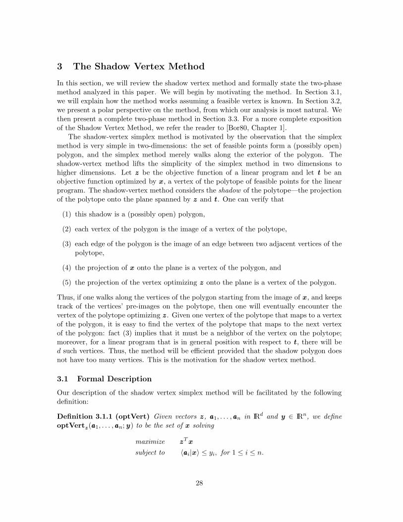
The shadow-vertex simplex method is motivated by the observation that the simplexmethod is very simple in two-dimensions: the set of feasible points form a (possibly open)polygon, and the simplex method merely walks along the exterior of the polygon. Theshadow-vertex method lifts the simplicity of the simplex method in two dimensions tohigher dimensions. Let z be the objective function of a linear program and let t be anobjective function optimized by x , a vertex of the polytope of feasible points for the linearprogram. The shadow-vertex method considers the shadow of the polytope—the projectionof the polytope onto the plane spanned by z and t . One can verify that
(1) this shadow is a (possibly open) polygon,
(2) each vertex of the polygon is the image of a vertex of the polytope,
(3) each edge of the polygon is the image of an edge between two adjacent vertices of thepolytope,
(4) the projection of x onto the plane is a vertex of the polygon, and
(5) the projection of the vertex optimizing z onto the plane is a vertex of the polygon.
Thus, if one walks along the vertices of the polygon starting from the image of x , and keepstrack of the vertices’ pre-images on the polytope, then one will eventually encounter thevertex of the polytope optimizing z . Given one vertex of the polytope that maps to a vertexof the polygon, it is easy to find the vertex of the polytope that maps to the next vertexof the polygon: fact (3) implies that it must be a neighbor of the vertex on the polytope;moreover, for a linear program that is in general position with respect to t , there will bed such vertices. Thus, the method will be efficient provided that the shadow polygon doesnot have too many vertices. This is the motivation for the shadow vertex method.
3.1 Formal Description
Our description of the shadow vertex simplex method will be facilitated by the followingdefinition:
Definition 3.1.1 (optVert) Given vectors z , aaa1, . . . ,aaan in IRd and y ∈ IRn, we defineoptVertz (aaa1, . . . ,aaan;y) to be the set of x solving
maximize z Tx
subject to 〈aaa i|x 〉 ≤ yi, for 1 ≤ i ≤ n.
28

Figure 1: A shadow of a polytope
If there are no such x , either because the program is unbounded or infeasible, we letoptVertz (aaa1, . . . ,aaan;y) be ∅. When aaa1, . . . ,aaan and y are understood, we will use thenotation optVertz .
We note that, for linear programs in general position, optVertz will either be empty orcontain one vertex.
Using this definition, we will give a description of the shadow vertex method assumingthat a vertex x 0 and a vector t are known for which optVertt = x 0. An algorithm thatworks without this assumption will be described in Section 3.3. Given t and z , we defineobjective functions interpolating between the two by
qλ = (1 − λ)t + λz .
The shadow-vertex method will proceed by varying λ from 0 to 1, and tracking optVertqλ.
We will denote the vertices encountered by x 0,x 1, . . . ,xk, and we will set λi so that x i ∈optVertqλ
for λ ∈ [λi, λi+1].As our main motivation for presenting the primal algorithm is to develop intuition in
the reader, we will not dwell on issues of degeneracy in its description. We will present apolar version of this algorithm with a proof of correctness in the next section.
29
primal shadow-vertex methodInput: aaa1, . . . ,aaan, y , z , and x 0 and t satisfying {x 0} =optVertt(aaa1, . . . ,aaan;y).
(1) Set λ0 = 0, and i = 0.
(2) Set λ1 to be maximal such that {x 0} = optVertqλfor λ ∈ [λ0, λ1].
(3) while λi+1 < 1,
(a) Set i = i + 1.
(b) Find an x i for which there exists a λi+1 > λi such that x i ∈optVertqλ
for λ ∈ [λi, λi+1]. If no such x i exists, return un-bounded.
(c) Let λi+1 be maximal such that x i ∈ optVertqλfor λ ∈ [λi, λi+1].
(4) return x i.
Step (b) of this algorithm deserves further explanation. Assuming that the linear pro-gram is in general position with respect to t , each vertex x i will have exactly d neighbors,and the vertex x i+1 will be one of these [Bor80, Lemma 1.3]. Thus, the algorithm can bedescribed as a simplex method. While one could implement the method by examining thesed vertices in turn, more efficient implementations are possible. For an efficient implemen-tation of this algorithm in tableau form, we point the reader to the exposition in [Bor80,Section 1.3].
3.2 Polar Description
Following Borgwardt [Bor80], we will analyze the shadow vertex method from a polar per-spective. This polar perspective is natural provided that all yi > 0. In this section, we willdescribe a polar variant of the shadow-vertex method that works under this assumption. Inthe next section, we will describe a two-phase shadow vertex method that uses this polarvariant to solve linear programs with arbitrary yis.
While it is not strictly necessary for the results in this paper, we remind the readerthat for a polytope P = {x : 〈x |aaa i〉 ≤ 1,∀i}, the polar of P is {y : 〈x |y〉 ≤ 1,∀x ∈ P}.An equivalent definition of the polar is ConvHull (0,aaa1, . . . ,aaan). We remark that P isbounded if and only if 0 is in the interior of ConvHull (aaa1, . . . ,aaan). The polar motivates:
Definition 3.2.1 (optSimp) For z and aaa1, . . . ,aaan in IRd and y ∈ IRn, yi > 0, we let
optSimpz (aaa1, . . . ,aaan;y) denote the set of I ∈([n]
d
)
such that AI has full rank, △ ((aaa i/yi)i∈I)is a facet of ConvHull (0,aaa1/y1, . . . ,aaan/yn) and z ∈ Cone ((aaa i)i∈I). When y is under-stood to be 1, we will use the notation optSimpz (aaa1, . . . ,aaan) When aaa1, . . . ,aaan and y areunderstood, we will use the notation optSimpz .
We remark that for y , z and aaa1, . . . ,aaan in general position, optSimpz (aaa1, . . . ,aaan;y)will be the empty set or contain just one set of indices I.
The following proposition follows from the duality theory of linear programming:
30
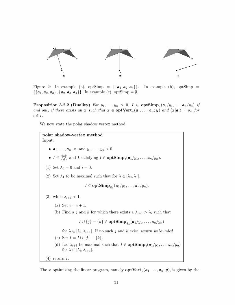
Figure 2: In example (a), optSimp = {{aaa1,aaa2,aaa3}}. In example (b), optSimp ={{aaa1,aaa2,aaa3} , {aaa2,aaa3,aaa4}}. In example (c), optSimp = ∅,
Proposition 3.2.2 (Duality) For y1, . . . , yn > 0, I ∈ optSimpz (aaa1/y1, . . . ,aaan/yn) ifand only if there exists an x such that x ∈ optVertz (aaa1, . . . ,aaan;y) and 〈x |aaa i〉 = yi, fori ∈ I.
We now state the polar shadow vertex method.
polar shadow-vertex methodInput:
• aaa1, . . . ,aaan, z , and y1, . . . , yn > 0,
• I ∈([n]
d
)
and t satisfying I ∈ optSimpt(aaa1/y1, . . . ,aaan/yn).
(1) Set λ0 = 0 and i = 0.
(2) Set λ1 to be maximal such that for λ ∈ [λ0, λ1],
I ∈ optSimpqλ(aaa1/y1, . . . ,aaan/yn).
(3) while λi+1 < 1,
(a) Set i = i + 1.
(b) Find a j and k for which there exists a λi+1 > λi such that
I ∪ {j} − {k} ∈ optSimpqλ(aaa1/y1, . . . ,aaan/yn)
for λ ∈ [λi, λi+1]. If no such j and k exist, return unbounded.
(c) Set I = I ∪ {j} − {k}.(d) Let λi+1 be maximal such that I ∈ optSimpt(aaa1/y1, . . . ,aaan/yn)
for λ ∈ [λi, λi+1].
(4) return I.
The x optimizing the linear program, namely optVertz (aaa1, . . . ,aaan;y), is given by the
31

equations 〈x |aaa i〉 = yi, for i ∈ I.Borgwardt [Bor80, Lemma 1.9] establishes that such j and k can be found in step (b) if
there exists an ǫ for which optSimpqλi+ǫ(aaa1/y1, . . . ,aaan/yn) 6= ∅. That the algorithm may
conclude that the program is unbounded if a j and k cannot be found in step (b) followsfrom:
Proposition 3.2.3 (Detecting unbounded programs) If there is an i and an ǫ > 0such that λi+ǫ < 1 and optSimpqλi+ǫ
(aaa1/y1, . . . ,aaan/yn) = ∅, then optSimpz (aaa1/y1, . . . ,aaan/yn) =
∅.
Proof optSimpqλi+ǫ(aaa1/y1, . . . ,aaan/yn) = ∅ if and only if qλi+ǫ 6∈ Cone (aaa1, . . . ,aaan).
The proof now follows from the facts that Cone (aaa1, . . . ,aaan) is a convex set and qλi+ǫ is apositive multiple of a convex combination of t and z .
The running time of the shadow-vertex method is bounded by the number of vertices inshadow of the polytope defined by the constraints of the linear program. Formally, this is
Definition 3.2.4 (Shadow) For independent vectors t and z , aaa1, . . . ,aaan in IRd and y ∈IRn, y > 0,
Shadowt ,z (aaa1, . . . ,aaan;y)def=
⋃
q∈Span(t ,z )
{
optSimpq (aaa1/y1, . . . ,aaan/yn)}
.
If y is understood to be 1, we will just write Shadowt ,z (aaa1, . . . ,aaan).
3.3 Two-Phase Method
We now describe a two-phase shadow vertex method that solves linear programs of form
maximize 〈z |x 〉subject to 〈aaai|x 〉 ≤ yi, for 1 ≤ i ≤ n. (LP )
There are three issues that we must resolve before we can apply the polar shadow vertexmethod as described in Section 3.2 to the solution of such programs:
(1) the method must know a feasible vertex of the linear program,
(2) the linear program might not even be feasible, and
(3) some yi might be non-positive.
The first two issues are standard motivations for two-phase methods, while the third ismotivated by the polar perspective from which we prefer to analyze the shadow vertexmethod. We resolve these issues in two stages. We first relax the constraints of LP toconstruct a linear program LP ′ such that
(a) the right-hand vector of the linear program is positive, and
(b) we know a feasible vertex of the linear program.
32

After solving LP ′, we construct another linear program, LP+, in one higher dimension thatinterpolates between LP and LP ′. LP+ has properties (a) and (b), and we can use theshadow vertex method on LP+ to transform the solution to LP ′ into a solution of LP .
Our two-phase method first chooses a d-set I to define the known feasible vertex of LP ′.The linear program LP ′ is determined by A, z and the choice of I. However, the magnitudeof the right-hand entries in LP ′ depends upon smin (AI). To reduce the chance that theseentries will need to be large, we examine several randomly chosen d-sets, and use the onemaximizing smin.
The algorithm then sets
M = 2⌈lg(maxi‖yi,aaai‖)⌉+2,
κ = 2⌊lg(smin(AI))⌋, and
y′i =
{
M for i ∈ I√dM2/4κ otherwise.
These define the program LP ′:
maximize 〈z |x 〉subject to 〈aaa i|x 〉 ≤ y′i, for 1 ≤ i ≤ n. (LP ′)
By Proposition 3.3.1, AI is a feasible basis for LP ′, and optimizes any objective functionof the form AIα, for α > 0. Our two-phase algorithm will solve LP ′ by starting the polarshadow-vertex algorithm at the basis I and the objective function AIα for a randomlychosen α satisfying
∑
αi = 1 and αi ≥ 1/d2, for all i.
Proposition 3.3.1 (Initial simplex of LP ′) For any α > 0, I = optSimpAIα(aaa1, . . . ,aaan;y ′).
Proof Let x ′ be the solution of the linear system⟨
aaai|x ′⟩
= y′i, for i ∈ I.
By Definition 2.2.3 and Proposition 2.2.4 (a),∥
∥x ′∥
∥ ≤∥
∥y ′I∥
∥
∥
∥A−1I
∥
∥ ≤ M√
d∥
∥A−1I
∥
∥ = M√
d/smin (AI) .
So, for all i 6∈ I,⟨
aaa i|x ′⟩
≤ (maxi
‖aaai‖)M√
d/smin (AI) < M2√
d/4κ.
Thus, for all i 6∈ I,⟨
aaa i|x ′⟩
< y′i,
and, by Definition 3.2.1, I = optSimpAIα(aaa1, . . . ,aaan;y ′).
We will now define a linear program LP+ that interpolates between LP ′ and LP . Thislinear program will contain an extra variable x0 and constraints of the form
〈aaai|x 〉 ≤(
1 + x0
2
)
yi +
(
1 − x0
2
)
y′i,
33

and −1 ≤ x0 ≤ 1. So, for x0 = 1 we see the original program LP while for x0 = −1 we getLP ′. Formally, we let
a+i =
((y′i − yi)/2,aaa i) for 1 ≤ i ≤ n(1, 0, . . . , 0) for i = 0(−1, 0, . . . , 0) for i = −1
y+i =
(y′i + yi)/2 for 1 ≤ i ≤ n1 for i = 01 for i = −1
z+ = (1, 0, . . . , 0),
and we define LP+ by
maximize⟨
z+|(x0,x )⟩
subject to⟨
a+i |(x0,x )
⟩
≤ y+i , for −1 ≤ i ≤ n, (LP+)
and we sety+ def
= (y+−1, . . . , y
+n ).
By Proposition 3.3.2,√
dM/4κ ≥ 1, so y′i ≥ M and y+i > 0, for all i. If LP is infeasible,
then the solution to LP+ will have x0 < 1. If LP is feasible, then the solution to LP+ willhave form (1,x ) where x is a feasible point for LP . If we use the shadow-vertex method tosolve LP+ starting from the appropriate initial vector, then x will be an optimal solutionto LP .
Proposition 3.3.2 (relation of M and κ) For M and κ as set by the algorithm,√
dM/4κ ≥1.
Proof By definition, κ ≤ smin (AI). On the other hand, smin (AI) ≤ ‖AI‖ ≤√
d maxi ‖aaai‖,by Proposition 2.2.4 (d). Finally, M ≥ 4maxi ‖aaai‖.
We now state and prove the correctness of the two-phase shadow vertex method.
34

two-phase shadow-vertex methodInput: A = (aaa1, . . . ,aaan), y , z .
(1) Let I = {I1, . . . , I3nd ln n} be a collection of randomly chosen sets in([n]
d
)
, and let I ∈ I be the set maximizing smin (AI).
(2) Set M = 2⌈lg(maxi‖yi,aaai‖)⌉+2 and κ = 2⌊lg(smin(AI ))⌋.
(3) Set y′i =
{
M for i ∈ I√dM2/4κ otherwise.
.
(4) Choose α uniformly at random from{
α :∑
αi = 1 and αi ≥ 1/d2}
.Set t ′ = AIα.
(5) Let J be the output of the polar shadow vertex algorithm on LP ′ oninput I and t ′. If LP ′ is unbounded, then return unbounded.
(6) Let ζ > 0 be such that
{−1} ∪ J ∈ optSimp(−ζ,z )
(
a+−1/y
+−1, . . . ,a
+n /y+
n
)
.
(7) Let K be the output of the polar shadow vertex algorithm on LP+ oninput {−1} ∪ J , (−ζ, z ).
(8) Compute (x0,x ) satisfying⟨
(x0,x )|a+i
⟩
= yi for i ∈ K.
(9) If x0 < 1, return infeasible. Otherwise, return x .
The following propositions prove the correctness of the algorithm.
Proposition 3.3.3 (Unbounded programs) The following are equivalent
(a) LP is unbounded;
(b) LP ′ is unbounded;
(c) there exists a 1 > λ > 0 such that optSimpλ(1,0)+(1−λ)(−ζ,z )
(
a+−1, . . . ,a
+n ;y+
)
= ∅;
(d) for all 1 > λ > 0, optSimpλ(1,0)+(1−λ)(−ζ,z )
(
a+−1, . . . ,a
+n ;y+
)
= ∅.
Proposition 3.3.4 (Bounded programs) If LP ′ is bounded and has solution J , then
(a) there exists ζ0 such that for all ζ > ζ0, {−1} ∪ J ∈ optSimp(−ζ,z )
(
a+−1, . . . ,a
+n ;y+
)
,
(b) If LP is feasible, then for K ′ ∈ optSimpz (aaa1, . . . ,aaan;y), there exists ξ0 such that forall ξ > ξ0, {0} ∪ K ′ ∈ optSimp(ξ,z )
(
a+−1, . . . ,a
+n ;y+
)
, and
(c) if we use the shadow vertex method to solve LP+ starting from {−1, J} and objectivefunction (−ζ, z ), then the output of the algorithm will have form {0} ∪ K ′, where K ′
is a solution to LP .
35

Proof of Proposition 3.3.3 LP is unbounded if and only if there exists a vector v
such that 〈z |v〉 > 0 and 〈aaa i|v〉 ≤ 0 for all i. The same holds for LP ′, and establishes theequivalence of (a) and (b). To show that (a) or (b) implies (d), observe
〈λ(1,0) + (1 − λ)(−ζ, z )|(0, v )〉 = (1 − λ) 〈z |v 〉 > 0, (8)⟨
a+i |(0, v )
⟩
= 〈aaai|v 〉 , for i = 1, . . . , n, (9)⟨
aaa+0 |(0, v )
⟩
= 0, and⟨
aaa+−1|(0, v )
⟩
= 0.
To show that (c) implies (a) and (b), note that a+0 and a+
−1 are arranged so that if for somev0 we have
⟨
a+i |(v0, v )
⟩
≤ 0, for −1 ≤ i ≤ n,
then v0 = 0. This identity allows us to apply (8) and (9) to show (c) implies (a) and (b).
Proof of Proposition 3.3.4 Let J be the solution to LP ′ and let x ′ = A−1J y ′J be the
corresponding vertex. We then have
⟨
x ′|aaa i
⟩
= y′i, for i ∈ J , and
⟨
x ′|aaa i
⟩
≤ y′i, for i 6∈ J.
Therefore, it is clear that
⟨
(−1,x ′)|a+i
⟩
= y+i , for i ∈ {−1} ∪ J , and
⟨
(−1,x ′)|a+i
⟩
≤ y+i , for i 6∈ {−1} ∪ J.
Thus, △(
a+−1, (a
+i )i∈J
)
is a facet of LP+. To see that there exists a ζ0 such that itoptimizes (−ζ, z ) for all ζ > ζ0, first observe that there exist αi > 0, for i ∈ J , such that∑
i∈J αiaaa i = z . Now, let (−ζ0, z ) =∑
i∈J αia+i . For ζ > ζ0, we have
(−ζ, z ) = (ζ − ζ0)a+−1 +
∑
i∈J
αia+i ,
which proves (−ζ, z ) ∈ Cone(
a+−1, (a
+i )i∈J
)
and completes the proof of (a).The proof of (b) is similar.To prove part (c), let K be as in step (7). Then, there exists a λk such that for all
λ ∈ (λk, 1),K = optSimp(1−λ)(−ζ,z )+λz+
(
a+−1, . . . ,a
+n ;y+
)
.
Let (x0,x ) satisfy⟨
(x0,x )|a+i
⟩
= y+i , for i ∈ K. Then, by Proposition 3.2.2,
(x0,x ) = optVert(1−λ)(−ζ,z )+λz+
(
a+−1, . . . ,a
+n ;y+
)
.
If x0 < 1, then LP was infeasible. Otherwise, let x ∗ = optVertz (aaa1, . . . ,aaan;y). By part(b), there exists ξ0 such that for all ξ > ξ0,
(1,x ∗) = optVert(ξ,z )
(
a+−1, . . . ,a
+n ;y+
)
.
36

For ξ = −ζ + λ/(1 − λ), we have
(ξ, z ) =1
1 − λ
(
(1 − λ)(−ζ, z ) + λz+)
.
So, as λ approaches 1, ξ = −ζ + λ/(1 − λ) goes to infinity and we have
optVert(1−λ)(−ζ,z )+λz+
(
a+−1, . . . ,a
+n ;y+
)
= optVert(ξ,z )
(
a+−1, . . . ,a
+n ;y+
)
,
which implies (x0,x ) = (1,x ∗).
Finally, we bound the number of steps taken in step (7) by the shadow size of a relatedpolytope:
Lemma 3.3.5 (Shadow path of LP+) Let aaa+−1, . . . ,aaa
+n and y+
−1, . . . , y+n be as defined in
LP+. Let ζ > 0 be such that {−1} ∪ J = optSimp(−ζ,z )
(
a+−1/y
+−1, . . . ,a
+n /y+
n
)
. Then thenumber of simplex steps made by the polar shadow vertex algorithm while solving LP+ frominitial basis {−1} ∪ J and vector (−ζ, z ) is at most
2 +∣
∣Shadow(0,z ),z+
(
a+1 /y+
1 , . . . ,a+n /y+
n
)∣
∣ .
Proof We will establish that {−1} ∈ I for the first step only. One can similarly provethat {0} ∈ I is only true at termination.
Let I ∈ optSimpqλ
(
a+−1/y
+−1, . . . ,a
+n /y+
n
)
have form {−1} ∪ L. As q0 = a+−1 ∈
Cone(
A{−1}∪L
)
, and Cone(
A{−1}∪L
)
is a convex set, we have qλ′ ∈ Cone(
A{−1}∪L
)
for all 0 ≤ λ′ ≤ λ. As [λi, λi+1] is exactly the set of λ optimized by △ (AI) in the ith stepof the polar shadow vertex method, I must be the initial set.
3.4 Discussion
We also note that our analysis of the two-phase algorithm actually takes advantage of thefact that κ and M have been set to powers of two. In particular, this fact is used to showthat there are not too many likely choices for κ and M . For the reader who would like todrop this condition, we briefly explain how the argument of Section 5 could be modified tocompensate: first, we could consider setting κ and M to powers of 1 + 1/poly(n, d, 1/σ).This would still result in a polynomially bounded number of choices for κ and M . Onecould then drop this assumption by observing that allowing κ and M to vary in a smallrange would not introduce too much dependency between the variables.
37

4 Shadow Size
In this section, we bound the expected size of the shadow of the perturbation of a polytopeonto a fixed plane. This is the main geometric result of the paper. The algorithmic resultsof this paper will rely on extensions of this theorem derived in Section 4.3.
Theorem 4.0.1 (Shadow Size) Let d ≥ 3 and n > d. Let z and t be independent vectorsin IRd, and let µ1, . . . , µn be Gaussian distributions in IRd of standard deviation σ centeredat points each of norm at most 1. Then,
Eaaa1,...,aaan
[|Shadowt ,z (aaa1, . . . ,aaan)|] ≤ D(n, d, σ), (10)
where
D(n, d, σ) =58, 888, 678 nd3
min(
σ, 1/3√
d ln n)6 ,
and aaa1, . . . ,aaan have density∏n
i=1 µi(aaa i).
The proof of Theorem 4.0.1, will use the following definitions.
Definition 4.0.2 (ang) For a vector q and a set S, we define
ang (q , S) = minx∈S
angle (q ,x ) ,
If S is empty, we set ang (q , ∅) = ∞.
Definition 4.0.3 (angq) For a vector q and points aaa1, . . . ,aaan in IRd, we define
angq (aaa1, . . . ,aaan) = ang(
q , ∂ △(
optSimpq (aaa1, . . . ,aaan)))
,
where ∂△(
optSimpq (aaa1, . . . ,aaan))
denotes the boundary of the simplex △(
optSimpq (aaa1, . . . ,aaan))
.
These definitions are arranged so that if the ray through q does not pierce the convexhull of aaa1, . . . ,aaan, then angq (aaa1, . . . ,aaan) = ∞.
In our proofs, we will make frequent use of the fact that it is very unlikely that aGaussian random variable is far from its mean. To capture this fact, we define:
Definition 4.0.4 (P) P is the set of (aaa1, . . . ,aaan) for which ‖aaai‖ ≤ 2, for all i.
Applying a union bound to Corollary 2.4.6, we obtain
Proposition 4.0.5 (Measure of P)
Pr [(aaa1, . . . ,aaan) ∈ P ] ≥ 1 − n(n−2.9d) = 1 − n−2.9d+1.
38

Proof of Theorem 4.0.1 We first observe that we can assume σ ≤ 1/3√
d ln n: ifσ > 1/3
√d ln n, then we can scale down all the data until σ = 1/3
√d ln n. As this could
only decrease the norms of the centers of the distributions, the theorem statement wouldbe unaffected.
Assume without loss of generality that z and t are orthogonal. Let
qθ = z sin(θ) + t cos(θ). (11)
We discretize the problem by using the intuitively obvious fact, which we prove as Lemma 4.0.6,that the left-hand of (10) equals
limm→∞
Eaaa1,...,aaan
∣
∣
∣
∣
∣
∣
∣
⋃
θ∈{ 2πm
, 2·2πm
,..., m·2πm }
{
optSimpqθ(aaa1, . . . ,aaan)
}
∣
∣
∣
∣
∣
∣
∣
.
Let Ei denote the event[
optSimpq2πi/m(aaa1, . . . ,aaan) 6= optSimpq2π((i+1) mod m)/m
(aaa1, . . . ,aaan)]
.
Then, for any m ≥ 2 and for all aaa1, . . . ,aaan,∣
∣
∣
∣
∣
∣
∣
⋃
θ∈{ 2πm
, 2·2πm
,..., m·2πm }
{
optSimpqθ(aaa1, . . . ,aaan)
}
∣
∣
∣
∣
∣
∣
∣
=
m∑
i=1
Ei(aaa1, . . . ,aaan).
We bound this sum by
E
[
m∑
i=1
Ei
]
= EP
[
∑
i
Ei
]
Pr [P ] + EP
[
∑
i
Ei
]
Pr[
P]
≤ EP
[
∑
i
Ei
]
+
(
n
d
)
n−2.9d+1
≤ EP
[
∑
i
Ei
]
+ 1
Thus, we will focus on bounding EP [∑
i Ei].
Observing that Ei implies[
angq2πi/m(aaa1, . . . ,aaan) ≤ 2π/m
]
, and applying linearity of
expectation, we obtain
EP
[
∑
i
Ei
]
=
m∑
i=1
PrP
[Ei]
≤m∑
i=1
PrP
[
angq2πi/m(aaa1, . . . ,aaan) <
2π
m
]
≤ 2π9, 372, 424 nd3
σ6by Lemma 4.0.7,
≤ 58, 888, 677 nd3
σ6.
39

Lemma 4.0.6 (Discretization in limit) Let z and t be orthogonal vectors in IRd, andlet µ1, . . . , µn be non-degenerate Gaussian distributions. Then,
Eaaa1,...,aaan
∣
∣
∣
∣
∣
∣
⋃
q∈Span(z ,t)
{
optSimpq (aaa1, . . . ,aaan)}
∣
∣
∣
∣
∣
∣
=
limm→∞
Eaaa1,...,aaan
∣
∣
∣
∣
∣
∣
∣
⋃
θ∈{ 2πm
, 2·2πm
,..., m·2πm }
{
optSimpqθ(aaa1, . . . ,aaan)
}
∣
∣
∣
∣
∣
∣
∣
, (12)
where qθ is as defined in (11).
Proof For a I ∈([n]
d
)
, let
FI(aaa1, . . . ,aaan) =
∫
θ
[
optSimpqθ(aaa1, . . . ,aaan) = I
]
dθ .
The left and right hand sides of (12) can differ only if there exists a δ > 0 such that for allǫ > 0,
Praaa1,...,aaan
[
∃I∣
∣
∣
I = optSimpqθ(aaa1, . . . ,aaan) for some θ, and
FI(aaa1, . . . ,aaan) < ǫ
]
≥ δ.
As there are only finitely many choices for I, this would imply the existence of a δ′ and aparticular I such that for all ǫ > 0,
Praaa1,...,aaan
[
I = optSimpqθ(aaa1, . . . ,aaan) for some θ, and
FI(aaa1, . . . ,aaan) < ǫ
]
≥ δ′.
As FI(aaa1, . . . ,aaan) = FI(AI) given that I = optSimpqθ(aaa1, . . . ,aaan) for some θ, this implies
that for all ǫ > 0,
Praaa1,...,aaan
[
I = optSimpqθ(AI) for some θ, and
FI(AI) < ǫ
]
≥ δ′. (13)
Note that I = optSimpqθ(AI) if and only if qθ ∈ Cone (AI). Now, let
G(AI) =
∫
θ[qθ ∈ Cone (AI)] (ang (qθ, ∂ △ (AI)) /π) dθ .
As G(AI) ≤ FI(AI), (13) implies that for all ǫ > 0
Praaa1,...,aaan
[
I = optSimpqθ(aaa1, . . . ,aaan) for some θ, and
G(AI) < ǫ
]
≥ δ′.
However, G is a continuous function, and therefore measurable, so this would imply
Praaa1,...,aaan
[
I = optSimpqθ(aaa1, . . . ,aaan) for some θ, and
G(AI) = 0
]
≥ δ′,
which is clearly false as the set of AI satisfying
40

• G(AI) = 0, and
• ∃θ : optSimpqθ(aaa1, . . . ,aaan) = {AI}
has co-dimension 1, and so has measure zero under the product distribution of non-degenerateGaussians.
Lemma 4.0.7 (Angle bound) Let d ≥ 3 and n > d. Let q be any unit vector and letµ1, . . . , µn be Gaussian measures in IRd of standard deviation σ ≤ 1/3
√d ln n centered at
points of norm at most 1. Then,
PrP
[
angq (aaa1, . . . ,aaan) < ǫ]
≤ 9, 372, 424 nd3
σ6ǫ
where aaa1, . . . ,aaan have densityn∏
i=1
µi(aaa i).
The proof will make use of the following definition:
Definition 4.0.8 (PjI ) For a I ∈
([n]d
)
and j ∈ I, we define P jI to be the set of aaa1, . . . ,aaad
satisfying
(1) For all q , if optSimpq (aaa1, . . . ,aaan) 6= ∅, then s ≤ 2, where s is the real number forwhich sq ∈ △
(
optSimpq (aaa1, . . . ,aaan))
,
(2) dist (aaai,aaak) ≤ 4, for i, k ∈ I − {j},
(3) dist(
aaaj,Aff(
AI−{j}))
≤ 4, and
(4) dist(
aaa⊥j ,aaa i
)
≤ 4, for all i ∈ I−{j}, where aaa⊥j is the orthogonal projection of aaaj onto
Aff(
AI−{j})
.
Proposition 4.0.9 (P ⊂ PjI ) For all j, I, P ⊂ P j
I .
Proof Parts (2), (3), and (4) follow immediately from the restrictions ‖aaa i‖ ≤ 2. To seewhy part (1) is true, note that sq lies in the convex hull of aaa1, . . . ,aaan, and so its norm, s,can be at most maxi ‖aaa i‖ ≤ 2, for (aaa1, . . . ,aaan) ∈ P .
Proof of Lemma 4.0.7 Applying a union bound twice, we write
PrP
[
angq (aaa1, . . . ,aaan) < ǫ]
≤∑
I
PrP
[
optSimpq (aaa1, . . . ,aaan) = I and
ang(q , ∂ △ (AI)) < ǫ
]
≤∑
I
d∑
j=1
PrP
[
optSimpq (aaa1, . . . ,aaan) = I and
ang(q ,△(
AI−{j})
) < ǫ
]
≤∑
I
d∑
j=1
PrP j
I
[
optSimpq (aaa1, . . . ,aaan) = I and
ang(q ,△(
AI−{j})
) < ǫ
]
/
PrP j
I
[P ]
41

(by Proposition 2.3.2)
≤∑
I
d∑
j=1
PrP j
I
[
optSimpq (aaa1, . . . ,aaan) = I and
ang(q ,△(
AI−{j})
) < ǫ
]
/
Pr [P ]
(by P ⊂ P jI )
≤ 1
1 − n−2.9d+1
∑
I
d∑
j=1
PrP j
I
[
optSimpq (aaa1, . . . ,aaan) = I and
ang(q ,△(
AI−{j})
) < ǫ
]
(by Proposition 4.0.5)
≤ 1
1 − n−2.9d+1
d∑
j=1
∑
I
PrP j
I
[
optSimpq (aaa1, . . . ,aaan) = I and
ang(q ,△(
AI−{j})
) < ǫ,
]
,
by changing the order of summation.We now expand the inner summation using Bayes’ rule to get
∑
I
PrP j
I
[
optSimpq (aaa1, . . . ,aaan) = I andang(q ,△
(
AI−{j})
) < ǫ
]
=∑
I
PrP j
I
[
optSimpq (aaa1, . . . ,aaan) = I]
·
PrP j
I
[
ang(q ,△(
AI−{j})
) < ǫ∣
∣
optSimpq (aaa1, . . . ,aaan) = I
]
(14)
As optSimpq (aaa1, . . . ,aaan) is a set of size zero or one with probability 1,
∑
I
Pr[
optSimpq (aaa1, . . . ,aaan) = I]
≤ 1;
from which we derive∑
I
PrP j
I
[
optSimpq (aaa1, . . . ,aaan) = I]
≤∑
I
Pr[
optSimpq (aaa1, . . . ,aaan) = I] /
Pr[
P jI
]
(by Proposition 2.3.2)
≤ 1
1 − n−2.9d+1
∑
I
Pr[
optSimpq (aaa1, . . . ,aaan) = I]
(by P ⊂ P jI and Proposition 4.0.5)
≤ 1
1 − n−2.9d+1.
42

So,
(14) ≤ 1
1 − n−2.9d+1.max
IPrP j
I
[
ang(q ,△(
AI−{j})
) < ǫ∣
∣
optSimpq (aaa1, . . . ,aaan) = I
]
.
Plugging this bound in to the first inequality derived in the proof, we obtain the bound of
PrP
[
angq (aaa1, . . . ,aaan) < ǫ]
≤ d
(1 − n−2.9d+1)2maxj,I
PrP j
I
[
ang(q ,△(
AI−{j})
) < ǫ∣
∣
optSimpq (aaa1, . . . ,aaan) = I
]
≤ d9, 372, 424 nd3
σ6ǫ, by Lemma 4.0.11, d ≥ 3 and n ≥ d + 1,
=9, 372, 424 nd3
σ6ǫ.
Definition 4.0.10 (Q) We define Q to be the set of (b1, . . . , bd) ∈ IRd−1 satisfying
(1) dist (b1,Aff (b2, . . . , bd)) ≤ 4,
(2) dist (bi, bj) ≤ 4 for all i, j ≥ 2,
(3) dist(
b⊥1 , b i
)
≤ 4 for all i ≥ 2, where b⊥1 is the orthogonal projection of b1 ontoAff (b2, . . . , bd), and
(4) 0 ∈ △ (b1, . . . , bd).
Lemma 4.0.11 (Angle bound given optSimp) Let µ1, . . . , µn be Gaussian measures inIRd of standard deviation σ ≤ 1/3
√d ln n centered at points of norm at most 1. Then
PrP 1
1,...,d
[
ang(q ,△ (aaa2, . . . ,aaad)) < ǫ∣
∣
optSimpq (aaa1, . . . ,aaan) = {1, . . . , d}
]
≤ 9, 371, 990 nd2ǫ
σ6(15)
where aaa1, . . . ,aaan have densityn∏
i=1
µi(aaa i).
Proof We begin by making the change of variables from aaa1, . . . ,aaad to ω, s, b1, . . . , bd
described in Corollary 2.5.3, and we recall that the Jacobian of this change of variables is
(d − 1)! 〈ω|q〉Vol (△ (b1, . . . , bd)) .
As this change of variables is arranged so that sq ∈ △ (aaa1, . . . ,aaad) if and only if 0 ∈△ (b1, . . . , bd), the condition that optSimpq (aaa1, . . . ,aaan) = {1, . . . , d} can be expressed as
[0 ∈ △ (b1, . . . , bd)]∏
j>d
[〈ω|aaaj〉 ≤ 〈ω|sq〉] .
43

Let x be any point on △ (aaa2, . . . ,aaad). Given that sq ∈ △ (aaa1, . . . ,aaad), conditions (3)and (4) for membership in P 1
1,...,d imply that
dist (sq ,x ) ≤ dist (aaa1,x ) ≤√
dist (aaa1,Aff (aaa2, . . . ,aaad))2 + dist
(
aaa⊥1 ,x)2 ≤ 4
√2,
where aaa⊥1 is the orthogonal projection of aaa1 onto Aff (aaa2, . . . ,aaad). So, Lemma 4.0.12 implies
ang (q ,△ (aaa2, . . . ,aaad)) ≥dist (sq ,Aff (aaa2, . . . ,aaad)) 〈ω|q〉
2 + 4√
2=
dist (0,Aff (b2, . . . , bd)) 〈ω|q〉2 + 4
√2
.
Finally, observe that (aaa1, . . . ,aaad) ∈ P 11,...,d is equivalent to the conditions (b1, . . . , bd) ∈
Q and s ≤ 2, given that optSimpq (aaa1, . . . ,aaad) = {1, . . . , d}. Now, the left-hand side of(15) can be bounded by
Prω,s≤2
(b1,...,bd)∈Q
[
dist (0,Aff (b2, . . . , bd)) 〈ω|q 〉2 + 4
√2
< ǫ
]
, (16)
where the variables have density proportional to
〈ω|q〉Vol (△ (b1, . . . , bd))
∏
j>d
∫
aaaj
[〈ω|aaaj〉 ≤ s 〈ω|q〉]µj(aaaj) daaaj
d∏
i=1
µi(Rωbi + sq).
As Lemma 4.1.1 implies
Prω,s≤2
(b1,...,bd)∈Q
[dist (0,Aff (b2, . . . , bd)) < ǫ] ≤ 900e2/3d2ǫ
σ4,
and Lemma 4.2.1 implies
maxs≤2,b1,...,bd∈Q
Prω
[〈ω|q〉 < ǫ] <
(
340nǫ
σ2
)2
,
we can apply Lemma 2.3.5 to prove
(16) ≤ 4 · (2 + 4√
2) ·(
900e2/3d2
σ4
)
(
340n
σ2
)
ǫ ≤ 9, 371, 990 nd2ǫ
σ6.
Lemma 4.0.12 (Division into distance and angle) Let x be a vector, let 0 < s ≤ 2,and let q and ω be unit vectors satisfying
(a) 〈ω|x − sq〉 = 0, and
(b) dist (x , sq) ≤ 4√
2.
44

Then,
angle (q ,x ) ≥ dist (x , sq) 〈ω|q〉2 + 4
√2
.
Proof Let r = x − sq . Then, (a) implies
〈ω|q〉2 +
⟨
r
‖r‖∣
∣
∣q
⟩2
≤ ‖q‖ = 1;
so,
〈r |q〉 ≤√
1 − 〈ω|q〉2 ‖r‖ .
Let h be the distance from x to the ray through q . Then,
h2 + 〈r |q〉2 = ‖r‖2 ;
so,h ≥ 〈ω|q〉 ‖r‖ = 〈ω|q〉dist (x , sq)
Now,
angle (q ,x ) ≥ sin(angle (q ,x )) =h
‖x‖ ≥ h
s + dist (x , sq)≥ h
2 + 4√
2≥ 〈ω|q〉dist (x , sq)
2 + 4√
2.
4.1 Distance
The goal of this section is to prove it is unlikely that 0 is near ∂ △ (b1, . . . , bd).
d1
d2
0
d3
h
h
d3
d1
d2
0
b3b2
b1
Figure 3: The change of variables in Lemma 4.1.2.
45

Lemma 4.1.1 (Distance bound) Let q be a unit vector and let µ1, . . . , µn be Gaussianmeasures in IRd of standard deviation σ ≤ 1/3
√d ln n centered at points of norm at most 1.
Then,
Prω,s≤2
(b1,...,bd)∈Q
[dist (0,Aff (b2, . . . , bd)) < ǫ] ≤ 900e2/3d2ǫ
σ4, (17)
where the variables have density proportional to
〈ω|q〉Vol (△ (b1, . . . , bd))
∏
j>d
∫
aaaj
[〈ω|aaaj〉 ≤ s 〈ω|q〉]µj(aaaj) daaaj
d∏
i=1
µi(Rωbi + sq).
Proof Note that if we fix ω and s, then the first and third terms in the density becomeconstant. For any fixed plane specified by (ω, s), Proposition 2.4.3 tells us that the induceddensity on bi remains a Gaussian of standard deviation σ and is centered at the projectionof the center of µi onto the plane. As the origin of this plane is the point sq , and s ≤ 2,these induced Gaussians have centers of norm at most 3. Thus, we can use Lemma 4.1.2 tobound the left-hand side of (17) by
maxω,s≤2
Pr(b1,...,bd)∈Q
[dist (0,Aff (b2, . . . , bd)) < ǫ] ≤ 900e2/3d2ǫ
σ4.
Lemma 4.1.2 (Distance bound in plane) Let µ1, . . . , µd be Gaussian measures in IRd−1.of standard deviation σ ≤ 1/3
√d ln n centered at points of norm at most 3. Then
Prb1,...,bd∈Q
[dist (0,Aff (b2, . . . , bd)) < ǫ] ≤ 900e2/3d2ǫ
σ4, (18)
where b1, . . . , bd have density proportional to
Vol (△ (b1, . . . , bd))d∏
i=1
µi(b i).
Proof In Lemma 4.1.3, we will prove it is unlikely that b1 is close to Aff (b2, . . . , bd).We will exploit this fact by proving that it is unlikely that 0 is much closer than b1 toAff (b2, . . . , bd). We do this by fixing the shape of △ (b1, . . . , bd), and then consideringslight translations of this simplex. That is, we make a change of variables to
h =1
d
d∑
i=1
bi
di = h − b i, for i ≥ 2.
The vectors d2, . . . ,dd specify the shape of the simplex, and h specifies its location. As thischange of variables is a linear transformation, its Jacobian is constant. For convenience, wealso define d1 = h − b1 = −∑i≥2 di.
46

It is easy to verify that
0 ∈ △ (b1, . . . , bd) ⇔ h ∈ △ (d1, . . . ,dd) ,
dist (0,Aff (b2, . . . , bd)) = dist (h ,Aff (d2, . . . ,dd)) ,
dist (b1,Aff (b2, . . . , bd)) = dist (d1,Aff (d2, . . . ,dd)) , and
Vol (△ (b1, . . . , bd)) = Vol (△ (d1, . . . ,dd)) .
Note that the relation between d1 and d2, . . . ,dd guarantees 0 ∈ △ (d1, . . . ,dd) for alld2, . . . ,dd. So, (b1, . . . , bd) ∈ Q if and only if (d1, . . . ,dd) ∈ Q and h ∈ △ (d1, . . . ,dd). Asd1 is a function of d2, . . . ,dd, we let Q′ be the set of d2, . . . ,dd for which (d1, . . . ,dd) ∈ Q.
So, the left-hand side of (18) equals
Pr(d2,...,dd)∈Q′
h∈△(d1,...,dd)
[dist (h ,Aff (d2, . . . ,dd)) < ǫ]
where h ,d2, . . . ,dd have density proportional to
Vol (△ (d1, . . . ,dd))
d∏
i=1
µi(h − di). (19)
Similarly, Lemma 4.1.3 can be seen to imply
Pr(d2,...,dd)∈Q′
h∈△(d1,...,dd)
[dist (d1,Aff (d2, . . . ,dd)) < ǫ] ≤(
ǫ3e2/3d
σ2
)3
≤(
ǫ3e2/3d
σ2
)2
(20)
under density proportional to (19). We take advantage of (20) by proving
maxd2,...,dd∈Q′
Prh∈△(d1,...,dd)
[
dist (h ,Aff (d2, . . . ,dd))
dist (d1,Aff (d2, . . . ,dd))< ǫ
]
<75dǫ
σ2, (21)
where h has density proportional to
d∏
i=1
µi(h − di).
Before proving (21), we point out that using Lemma 2.3.5 to combine (20) and (21), weobtain
Pr(d2,...,dd)∈Q′
h∈△(d1,...,dd)
[dist (h ,Aff (d2, . . . ,dd) < ǫ)] ≤ 900e2/3d2ǫ
σ4,
from which the lemma follows.To prove (21), we let
Uǫ =
{
h ∈ △ (d1, . . . ,dd) :dist (h ,Aff (d2, . . . ,dd))
dist (d1,Aff (d2, . . . ,dd))≥ ǫ
}
,
47

and we set ν(h) =∏d
i=1 µi(h − di). Under this notation, the probability in (21) is equal to
(ν(U0) − ν(Uǫ))/ν(U0).
To bound this ratio, we construct an isomorphism from U0 to Uǫ. The natural isomorphism,which we denote Φǫ, is the map that contracts the simplex by a factor of (1 − ǫ) at d1.To use this isomorphism to compare the measures of the sets, we use the facts that ford1, . . . ,dd ∈ Q and h ∈ △ (d1, . . . ,dd),
(a) ‖h − di‖ ≤ maxi,j ‖di − dj‖ ≤ 4√
2, so the distance from h − di to the center of itsdistribution is at most ‖h − di‖ + 3 ≤ 4
√2 + 3;
(b) dist (h ,Φǫ(h)) ≤ ǫmaxi dist (d1,di) ≤ 4√
2ǫ
to apply Lemma 2.4.2 to show that for all h ∈ △ (d1, . . . ,dd),
µi(Φǫ(h) − di)
µi(h − di)≥ e−
3·4√
2(4√
2+3)ǫ
2σ2 = e−(48+18
√2)ǫ
σ2 .
So,
minh∈△(d1,...,dd)
ν(Φǫ(h))
ν(h)= min
h∈△(d1,...,dd)
d∏
i=1
µi(Φǫ(h) − di)
µi(h − di)≥ e−
(48+18√
2)dǫ
σ2 ≥ 1−(48 + 18√
2)dǫ
σ2.
(22)As the Jacobian
∣
∣
∣
∣
∂Φǫ(h)
∂h
∣
∣
∣
∣
= (1 − ǫ)d ≥ 1 − dǫ,
using the change of variables x = Φǫ(h) we can compute
ν(Uǫ) =
∫
x∈Uǫ
ν(x ) dx =
∫
h∈U0
ν(Φǫ(h))
∣
∣
∣
∣
∂Φǫ(h)
∂h
∣
∣
∣
∣
dh ≥ (1−dǫ)
∫
h∈U0
ν(Φǫ(h)) dh . (23)
So,
ν(Uǫ)
ν(U0)≥
(1 − dǫ)∫
h∈U0ν(Φǫ(h)) dh
∫
h∈U0ν(h) dh
by (23)
≥ (1 − dǫ)
(
minh∈△(d1,...,dd)
ν(Φǫ(h))
ν(h)
)
∫
h∈U0dh
∫
h∈U0dh
≥ (1 − dǫ)
(
1 − (48 + 18√
2)dǫ
σ2
)
by (22)
≥ 1 − 75dǫ
σ2, as σ ≤ 1.
(21) now follows from (ν(U0) − ν(Uǫ))/ν(U0) < 75dǫσ2 .
48

c3 c2 c1
b3 b2
τt
l
b1
Figure 4: The change of variables in Lemma 4.1.3.
Lemma 4.1.3 (Height of simplex) Let µ1, . . . , µd be Gaussian measures in IRd−1 of stan-dard deviation σ ≤ 1/3
√d ln n centered at points of norm at most 3. Then
Prb1,...,bd∈Q
[dist (b1,Aff (b2, . . . , bd) < ǫ)] ≤(
3ǫe2/3d
σ2
)3
where b1, . . . , bd have density proportional to
Vol (△ (b1, . . . , bd))
d∏
i=1
µi(b i).
Proof We begin with a simplifying change of variables. As in Theorem 2.5.2, we let
(b2, . . . , bd) = (Rτc2 + tτ , . . . ,Rτcd + tτ ) ,
where τ ∈ Sd−2 and t ≥ 0 specify the plane through b2, . . . , bd, and c2, . . . , cd ∈ IRd−2
denote the local coordinates of these points on that plane. Recall that the Jacobian ofthis change of variables is Vol (△ (c2, . . . , cd)). Let l = −〈τ |b1〉, and let c1 denote thecoordinates in IRd−2 of the projection of b1 onto the plane specified by τ and t. Note thatl ≥ 0. In this notation, we have
dist (b1,Aff (b2, . . . , bd)) = l + t.
The Jacobian of the change from b1 to (l, c1) is 1 as the transformation is just an orthogonalchange of coordinates. The conditions for (b1, . . . , bd) ∈ Q translate into the conditions
49

(a) dist (ci, cj) ≤ 4 for all i 6= j;
(b) (l + t) ≤ 4; and
(c) 0 ∈ △ (b1, . . . , bd).
Let R denote the set of c1, . . . , cd satisfying the first condition. As the lemma is vacuouslytrue for ǫ ≥ 4, we will drop the second condition and note that doing so cannot decreasethe probability that (t + l) < ǫ. Thus, our goal is to bound
Prτ,t,l,(c1,...,cd)∈R
[(l + t) < ǫ] , (24)
where the variables have density proportional to2
[0 ∈ △ (b1, . . . , bd)]Vol (△ (b1, . . . , bd))Vol (△ (c2, . . . , cd))
d∏
i=1
µi(bi).
As Vol (△ (b1, . . . , bd)) = (l + t)Vol (△ (c1, . . . , cd)) /d, this is the same as having densityproportional to
(l + t) [0 ∈ △ (b1, . . . , bd)]Vol (△ (c2, . . . , cd))2
d∏
i=1
µi(b i).
Under a suitable system of coordinates, we can express b1 = (−l, c1) and bi = (t, ci) fori ≥ 2. The key idea of this proof is that multiplying the first coordinates of these points by aconstant does not change whether or not 0 ∈ △ (b1, . . . , bd); so, we can determine whether0 ∈ △ (b1, . . . , bd) from the data (l/t, c1, . . . , cd). Thus, we will introduce a new variableα, set l = αt, and let S denote the set of (α, c1, . . . , cd) for which 0 ∈ △ (b1, . . . , bd) and(c1, . . . , cd) ∈ R. This change of variables from l to α incurs a Jacobian of ∂l
∂α = t, so (24)equals
Prτ ,t,(α,c1,...,cd)∈S
[(1 + α)t < ǫ] ,
where the variables have density proportional to
t2(1 + α)Vol (△ (c2, . . . , cd))2 µ1(−αt, c1)
d∏
i=2
µi(t, ci).
We upper bound this probability by
maxτ ,(α,c1,...,cd)∈S
Prt
[(1 + α)t < ǫ] ≤ maxτ,(α,c1,...,cd)∈S
Prt
[max(1, α)t < ǫ] ,
where t has density proportional to
t2µ1(−αt, c1)
d∏
i=2
µi(t, ci).
2While we keep terms such as b1 in the expression of the density, they should be interpreted as functions
of τ , t, l, c1, . . . , cd.
50
For c1, . . . , cd fixed, the points (−αt, c1), (t, c2), . . . , (t, cd) become univariate Gaussians ofstandard deviation σ and mean of absolute value at most 3. Let t0 = σ2/(3max(1, α)d).Then, for t in the range [0, t0], −αt is at most 3+αt0 from the mean of the first distributionand t is at most 3 + t0 from the means of the other distributions. We will now observe thatif t is restricted to a sufficiently small domain, then the densities of these Gaussians willhave bounded variation. In particular, Lemma 2.4.2 implies that
maxt∈[0,t0] µ1(−αt, c1)∏d
i=2 µi(t, ci)
mint∈[0,t0] µ1(−αt, c1)∏d
i=2 µi(t, ci)≤ e3(3+αt0)αt0/2σ2
d∏
i=2
e3(3+t0)t0/2σ2
≤ e9αt0/2σ2
(
d∏
i=2
e9t0/2σ2
)
· e3(αt0)2/2σ2
(
d∏
i=2
e3t20/2σ2
)
≤ e3/2d
(
d∏
i=2
e3/2d
)
· eσ2/6d2
(
d∏
i=2
eσ2/6d2
)
≤ e3/2 · e1/6d
≤ e2.
Thus, we can now apply Lemma 2.3.7 to show that
Prt
[t < ǫ] < e2
(
3ǫ(max(1, α)d
σ2
)3
,
from which we conclude
Prt
[max(1, α)t < ǫ] <
(
3ǫe2/3d
σ2
)3
.
4.2 Angle of q to ω
Lemma 4.2.1 (Angle of incidence) Let d ≥ 3 and n > d. Let µ1, . . . , µn be Gaussiandensities in IRd of standard deviation σ centered at points of norm at most 1 in IRd. Lets ≤ 2 and let (b1, . . . , bd) ∈ Q. Then,
Prω
[〈ω|q〉 < ǫ] <
(
340ǫn
σ2
)2
, (25)
where ω has density proportional to
〈ω|q〉
∏
j>d
∫
aaaj
[〈ω|aaaj〉 ≤ s 〈ω|q〉]µj(aaaj) daaaj
d∏
i=1
µi(Rωbi + sq).
51

Proof First note that the conditions for (b1, . . . , bd) to be in Q imply that for 1 ≤ i ≤ d,b i has norm at most
√
(4)2 + (4)2 = 4√
2 by properties (1), (3) and (4) of Q.As in Proposition 2.5.4, we change ω to (c,ψ), where c = 〈ω|q〉 and ψ ∈ Sd−2.The
Jacobian of this change of variables is
(1 − c2)(d−3)/2.
In these variables, the bound follows from Lemma 4.2.2.
Lemma 4.2.2 (Angle of incidence, II) Let d ≥ 3 and n > d. Let µd+1, . . . , µn be Gaus-sian densities in IRd of standard deviation σ centered at points of norm at most 1 in IRd.Let s ≤ 2, and let b1, . . . , bd each have norm at most 4
√2. Let ψ ∈ Sd−2. Then
Pr [c < ǫ] <
(
340ǫn
σ2
)2
,
where c has density proportional to
(1− c2)(d−3)/2 · c ·
∏
j>d
∫
aaaj
[〈ωψ,c|aaaj〉 ≤ s 〈ωψ,c|q〉] µj(aaaj) daaaj
d∏
i=1
µi(Rωψ ,cbi + sq) (26)
Proof Let
ν1(c) = (1 − c2)(d−3)/2,
ν2(c) =∏
j>d
∫
aaaj
[〈ωψ,c|aaaj〉 ≤ s 〈ωψ,c|q〉]µj(aaaj) daaaj , and
ν3(c) =
d∏
i=1
µi(Rωψ,cb i + sq).
Then, the density of c is proportional to
(26) = c · ν1(c)ν2(c)ν3(c).
Let
c0 =σ2
240n. (27)
We will show that, for c between 0 and c0, the density will vary by a factor no greater than2. We begin by letting θ0 = π/2 − arccos(c0), and noticing that a simple plot of the arccosfunction reveals c0 < 1/26 implies
θ0 ≤ 1.001c0. (28)
So, as c varies in the range [0, c0], ωψ,c travels in an arc of angle at most θ0 and thereforetravels a distance at most θ0. As c = 〈q |ωψ,c〉, we can apply Lemma 4.2.3 to show
min0≤c≤c0 ν2(c)
max0≤c≤c0 ν2(c)≥ 1 − 8n(1 + s)θ0
3σ2≥ 1 − 24nθ0
3σ2≥ 1 − 1.001
30, (29)
52

by (27) and (28).We similarly note that as c varies between 0 and c0, the point Rωψ,c
b i + sq moves adistance of at most
θ0 ‖b i‖ ≤ 4√
2θ0.
As this point is at distance at most
1 + s + ‖b i‖ ≤ 4√
2 + 3
from the center of µi, Lemma 2.4.2 implies
min0≤c≤c0 µi(Rωψ,cb i + sq)
max0≤c≤c0 µi(Rωψ,cb i + sq)
≥ e−(3(4√
2+3)4√
2θ0)/2σ2 ≥ e−147θ0/σ2.
So,
min0≤c≤c0 ν3(c)
max0≤c≤c0 ν3(c)≥ e−147dθ0/σ2 ≥ e−148/240, (30)
by (27) and (28) and d ≤ n.Finally, we note that
1 ≥ ν1(c) = (1 − c2)(d−3)/2 ≥ (1 − 1/26d)(d−3)/2 ≥(
1 − 1
52
)
. (31)
So, combining equations (29), (30), and (31), we obtain
min0≤c≤c0 ν1(c)ν2(c)ν3(c)
max0≤c≤c0 ν1(c)ν2(c)ν3(c)≥(
1 − 1
52
)
e−148240
(
1 − 1.001
30
)
≥ 1/2.
We conclude by using Lemma 2.3.7 to show
Prc
[c < ǫ] ≤ 2(ǫ/c0)2 = 2
(
240ǫn
σ2
)2
≤(
340ǫn
σ2
)2
.
Lemma 4.2.3 (Points under plane) For n > d, let µd+1, . . . , µn be Gaussian distribu-tions in IRd of standard deviation σ centered at points of norm at most 1. Let s ≥ 0 and letω1 and ω2 be unit vectors such that 〈ω1|q〉 and 〈ω2|q 〉 are non-negative. Then,
∏
j>d
∫
aaaj[〈ω2|aaaj〉 ≤ s 〈ω2|q〉]µj(aaaj) daaaj
∏
j>d
∫
aaaj[〈ω1|aaaj〉 ≤ s 〈ω1|q〉]µj(aaaj) daaaj
≥ 1 − 8n(1 + s) ‖ω1 − ω2‖3σ2
.
Proof As the integrals in the statement of the lemma are just the integrals of Gaussianmeasures over half-spaces, they can be reduced to univariate integrals. If µj is centered ataj , then
∫
aaaj
[〈ω1|aaaj〉 ≤ s 〈ω1|q〉] µj(aaaj) daaaj =
(
1√2πσ
)d ∫
aaaj
[〈ω1|aaaj〉 ≤ s 〈ω1|q〉] e−‖aaaj−aj‖2/2σ2daaaj
=
(
1√2πσ
)d ∫
gj
[⟨
ω1|g j + aj
⟩
≤ s 〈ω1|q〉]
e−‖gj‖2/2σ2
dg j ,
53

(setting g j = aaaj − aj)
=
(
1√2πσ
)d ∫
gj
[⟨
ω1|g j
⟩
≤ 〈ω1|sq − aj〉]
e−‖gj‖2/2σ2
dg j
=1√2πσ
∫ t=〈ω1|sq−aj〉
t=−∞e−t2/2σ2
dt
(by Proposition 2.4.4)
=1√2πσ
∫ t=∞
t=−〈ω1|sq−aj〉e−t2/2σ2
dt .
As ‖aj‖ ≤ 1, we know
−〈ω1|sq − aj〉 = −〈ω1|sq〉 + 〈ω1|aj〉 ≤ 〈ω1|aj〉 ≤ 1 (32)
Similarly,
∣
∣− 〈ω1|sq − a j〉 + 〈ω2|sq − aj〉∣
∣ =∣
∣− 〈ω1 − ω2|sq − aj〉∣
∣
≤ ‖ω1 −ω2‖ ‖sq − a j‖ (33)
≤ ‖ω1 −ω2‖ (s + 1). (34)
Thus, by applying Lemma 2.4.11 to (32) and (34), we obtain
∫
aaaj[〈ω2|aaaj〉 ≤ s 〈ω2|q〉] µj(aaaj) daaaj
∫
aaaj[〈ω1|aaaj〉 ≤ s 〈ω1|q〉] µj(aaaj) daaaj
=
∫ t=∞t=−〈ω2|sq−aj〉 e
−t2/2σ2dt .
∫ t=∞t=−〈ω1|sq−aj〉 e
−t2/2σ2dt .
≥(
1 − 8(1 + s) ‖ω1 − ω2‖3σ2
)
.
Thus,
∏
j>d
∫
aaaj[〈ω2|aaaj〉 ≤ s 〈ω2|q〉]µj(aaaj) daaaj
∏
j>d
∫
aaaj[〈ω1|aaaj〉 ≤ s 〈ω1|q〉]µj(aaaj) daaaj
≥(
1 − 8(1 + s) ‖ω1 − ω2‖3σ2
)n−d
≥(
1 − 8n(1 + s) ‖ω1 − ω2‖3σ2
)
.
4.3 Extending the shadow bound
In this section, we relax the restrictions made in the statement of Theorem 4.0.1. Theextensions of Theorem 4.0.1 are needed in the proof of Theorem 5.0.1.
We begin by removing the restrictions on where the distributions are centered in theshadow bound.
54

Corollary 4.3.1 (‖aaai‖ free) Let z and t be unit vectors and let aaa1, . . . ,aaan be Gaussianrandom vectors in IRd of standard deviation σ ≤ 1/3
√d ln n centered at points a1, . . . , an.
Then,
E [Shadowz ,t (aaa1, . . . ,aaan)] ≤ D(
d, n,σ
max (1,maxi ‖a‖)
)
where D(d, n, σ) is as given in Theorem 4.0.1.
Proof Let k = maxi ‖a i‖. Assume without loss of generality that k ≥ 1, and let bi = aaai/kfor all i. Then, bi is a Gaussian random variable of standard deviation (σ/k) centered at apoint of norm at most 1. So, Theorem 4.0.1 implies
E [Shadowz ,t (b1, . . . , bn)] ≤ D(
d, n,σ
k
)
.
On the other hand, the shadow of the polytope defined by the b is can be seen to be a dilationof the polytope defined by the aaais: the division of the b is by a factor of k is equivalent tothe multiplication of x by k. So, we may conclude that for all aaa1, . . . ,aaan,
|Shadowz ,t (aaa1, . . . ,aaan)| = |Shadowz ,t (b1, . . . , bn)| .
Corollary 4.3.2 (Gaussians free) Let z and t be unit vectors and let aaa1, . . . ,aaan be Gaus-sian random vectors in IRd with covariance matrices M 1, . . . ,M n centered at points a1, . . . , an,respectively. If the eigenvalues of each M i lie between σ2 and 1/9d ln n, then
E [Shadowz ,t (aaa1, . . . ,aaan)] ≤ D(
d, n,σ
1 + maxi ‖a‖
)
+ 1
where D(d, n, σ) is as given in Theorem 4.0.1.
Proof By Proposition 2.4.1, each aaa i can be expressed as
aaa i = a i + g i + g i,
where g i is a Gaussian random vector of standard deviation σ centered at the origin and g i
is a Gaussian random vector centered at the origin with covariance matrix M 0i = M i−σ2I,
each of whose eigenvalues is at most 1/9d ln n. Let a i = a i + g i. If ‖a i‖ ≤ 1 + ‖a i‖, for alli, then we can apply Corollary 4.3.1 to show
Eg1,...,gn
[Shadowz ,t (aaa1, . . . ,aaan)] ≤ D(
d, n,σ
max (1,maxi ‖a‖)
)
≤ D(
d, n,σ
1 + maxi ‖a‖
)
.
On the other hand, Corollary 2.4.6 implies
Prg1,...,gn
[∃i : ‖a i‖ > 1 + ‖a i‖] ≤ 0.0015
(
n
d
)−1
55

So, using Lemma 2.3.3 and Shadowz ,t (aaa1, . . . ,aaan) ≤(n
d
)
, we can show
Eg1,...,gn
[
Eg1,...,gn
[Shadowz ,t (aaa1, . . . ,aaan)]
]
≤ D(
d, n,σ
1 + maxi ‖a‖
)
+ 1.
from which the Corollary follows.
Corollary 4.3.3 (yi free) Let y ∈ IRn be a positive vector. Let z and t be unit vectorsand let aaa1, . . . ,aaan be Gaussian random vectors in IRd with covariance matrices M 1, . . . ,M n
centered at points a1, . . . , an, respectively. If the eigenvalues of each M i lie between σ2 and1/9d ln n, then
E [Shadowz ,t (aaa1, . . . ,aaan) ;y ] ≤ D(
d, n,σ
(1 + maxi ‖a i‖)(maxi yi)/(mini yi)
)
+ 1
where D(d, n, σ) is as given in Theorem 4.0.1.
Proof Nothing in the statement is changed if we rescale the yis. So, assume without lossof generality that mini yi = 1.
Let b i = aaa i/yi. Then bi is a Gaussian random vector with covariance matrix M i/y2i
centered at a point of norm at most ‖aaa i‖ /yi ≤ ‖aaa i‖. Then, the eigenvalues of each M i
lie between σ2/y2i and 1/(9d ln ny2
i ) ≤ 1/9d ln n, so we may complete the proof by applyingCorollary 4.3.2.
56

5 Smoothed Analysis of a Two-Phase Simplex Algorithm
In this section, we will analyze the smoothed complexity of the two-phase shadow-vertexsimplex method introduced in Section 3.3. The analysis of the algorithm will use as a black-box the bound on the expected sizes of shadows proved in the previous section. However,the analysis is not immediate from this bound.
The most obvious difficulty in applying the shadow bound to the analysis of an algorithmis that, in the statement of the shadow bound, the plane onto which the polytope wasprojected to form the shadow was fixed, and unrelated to the data defining the polytope.However, in the analysis of the shadow-vertex algorithm, the plane onto which the polytopeis projected will necessarily depend upon data defining the linear program. This is thedominant complication in the analysis of the number of steps taken to solve LP ′.
Another obstacle will stem from the fact that, in the analysis of LP+, we need toconsider the expected sizes of shadows of the convex hulls of points of the form a+
i /y+i ,
which do not have a Gaussian distribution. In our analysis of LP+, we essentially handlethis complication by demonstrating that in almost every small region the distribution canbe approximated by some Gaussian distribution.
The last issue we need to address is that if smin (AI) is too small, then the resultingvalues for y′i and y+
i can be too large. In Section 5.1 we resolve this problem by proving thatone of 3nd ln n randomly chosen I will have reasonable smin (AI) with very high probability.Having a reasonable smin (AI) is also essential for the analysis of LP ′.
As our two-phase shadow-vertex simplex algorithm is randomized, we will measure itsexpected complexity on each input. For an input linear program specified by A, y and z ,we let
C(A,y , z )
denote the expected number of simplex steps taken by the algorithm on input (A,y , z ). Asthis expectation is taken over the choices for I and α, and can be divided into the numberof steps taken to solve LP+ and LP ′, we introduce the functions
S ′z (A,y ,I,α),
to denote the number of simplex steps taken by the algorithm in step (5) to solve LP ′ fora given A, y , I and α, and
S+z (A,y ,I) + 2
to denote the number of simplex steps3 taken by the algorithm in step (7) to solve LP+
for a given A, y and I. We note that the complexity of the second phase does not dependupon α, however it does depend upon I as I affects the choice of κ and M . We have
C(A,y , z ) ≤ EI,α
[
S ′z (A,y ,I,α)]
+ EI,α
[
S+z (A,y ,I,α)
]
+ 2.
Theorem 5.0.1 (Main) There exists a polynomial P and a constant σ0 such that for everyn > d ≥ 3, A = [aaa1, . . . , aaan] ∈ IRn×d, y ∈ IRn and z ∈ IRd, and σ > 0,
EA,y
[C(A,y , z )] ≤ min
(
P(d, n, 1/min(σ, σ0)),
(
n
d
)
+
(
n
d + 1
)
+ 2
)
,
3The seemingly odd appearance of +2 in this definition is explained by 3.3.5.
57

where A is a Gaussian random matrix centered at A of standard deviation σ maxi ‖(yi, aaa i)‖,and y is a Gaussian random vector centered at y of standard deviation σ maxi ‖(yi, aaa i)‖.
Proof We first observe that the behavior of the algorithm is unchanged if one multipliesA and y by a power of two. That is,
C(A,y , z ) = C(2kA, 2ky , z ),
for any integer k. When A and y are Gaussian random variables centered at A and y ofstandard deviation σ maxi ‖(yi, aaa i)‖, 2kA and 2ky are Gaussian random variables centeredat 2kA and 2ky of standard deviation σ maxi
∥
∥(2kyi, 2kaaa i)
∥
∥. Accordingly, we may assumewithout loss of generality in our analysis that maxi ‖(yi, aaa i)‖ ∈ (1/2, 1].
The Theorem now follows from Proposition 5.0.2 and Lemmas 5.2.1 and 5.3.1.
Before proceeding with the proof of Theorem 5.0.1, we state a trivial upper bound onS ′ and S+:
Proposition 5.0.2 (trivial shadow bounds) For all A, y , z , I and α:
S ′z (A,y ,I,α) ≤(
n
d
)
and S+z (A,y ,I,α) ≤
(
n
d + 1
)
.
Proof The bound on S ′ follows from the fact that there are(n
d
)
d-subsets of [n]. Thebound on S+ follows from the observation in Lemma 3.3.5 that the number of steps takenby the second phase is at most 2 plus the number of (d + 1)-subsets of [n].
58

5.1 Many Good Choices
For a Gaussian random d-by-d matrix (aaa1, . . . ,aaad), it is possible to show that the probabilitythat the smallest singular value of (aaa1, . . . ,aaad) is less than ǫ is at most O(d1/2ǫ). In thissection, we consider the probability that almost all of the d-by-d minors of a d-by-n matrix(aaa1, . . . ,aaan) have small singular value. If the events for different minors were independent,then the proof would be straightforward. However, distinct minors may have significantoverlap. While we believe stronger concentration results should be obtainable, we haveonly been able to prove:
Lemma 5.1.1 (Many good choices) For n > d ≥ 3, let aaa1, . . . ,aaan be Gaussian randomvariables in IRd of standard deviation σ centered at points of norm at most 1. Let A =(aaa1, . . . ,aaan). Then, we have
Praaa1,...,aaan
∑
I∈([n]d )
[smin (AI) ≤ κ0] ≥(
1 − 1
n
)(
n
d
)
≤ n−d + n−n+d−1 + n−2.9d+1,
where
κ0def=
σ min(1, σ)
12d2n7√
ln n. (35)
In the analyses of LP ′ and LP+, we use the following consequence of Lemma 5.1.1,whose statement is facilitated by the following notation for a set of d-sets, I
I(A)def= argmaxI∈I (smin (AI)) .
Corollary 5.1.2 (probability of small smin
(
AI(A)
)
) For n > d ≥ 3, let aaa1, . . . ,aaan be
Gaussian random variables in IRd of standard deviation σ centered at points of norm atmost 1, and let A = (aaa1, . . . ,aaan). For I a set of 3nd ln n randomly chosen d-subsets of [n],
PrA,I
[
smin
(
AI(A)
)
≤ κ0
]
≤ 0.417
(
n
d
)−1
.
59

Proof
PrA,I
[
smin
(
AI(A)
)
≤ κ0
]
= PrA,I
[∀I ∈ I : smin (AI) ≤ κ0]
≤ PrA
∑
I∈([n]d )
[smin (AI) ≤ κ0] <
(
1 − 1
n
)(
n
d
)
+ PrI,A
∀I ∈ I : smin (AI) ≤ κ0
∣
∣
∣
∣
∣
∑
I∈([n]d )
[smin (AI) ≤ κ0] ≥(
1 − 1
n
)(
n
d
)
≤ n−d + n−n+d−1 + n−2.9d+1 +
(
1 − 1
n
)|I|, by Lemma 5.1.1
≤ n−d + n−n+d−1 + n−2.9d+1 + n−3d, as |I| = 3nd ln n,
≤ 0.417
(
n
d
)−1
,
for n > d ≥ 3.
We also use the following corollary, which states that it is highly unlikely that κ fallsoutside the set K, which we now define:
K ={
2⌊lg(x)⌋ : κ0 ≤ x ≤√
d + 3d√
ln nσ}
. (36)
Corollary 5.1.3 (probability of κ in K) For n > d ≥ 3, let aaa1, . . . ,aaan be Gaussianrandom variables in IRd of standard deviation σ centered at points of norm at most 1, andlet A = (aaa1, . . . ,aaan). For I a set of 3nd ln n randomly chosen d-subsets of [n],
PrA,I
[
2⌊lg(smin(AI(A)))⌋ 6∈ K]
≤ 0.42
(
n
d
)−1
.
ProofIt follows from Corollary 5.1.2 that
PrA,I
[
smin
(
AI(A)
)
≤ κ0
]
≤ 0.417
(
n
d
)−1
.
On the other hand, assmin (AI) ≤ ‖AI‖ ≤
√dmax
i‖aaai‖ ,
PrA,I
[
smin
(
AI(A)
)
≥√
d(
1 + 3√
d ln nσ)]
≤ PrA
[
maxi
‖aaa i‖ ≥ 1 + 3√
d ln nσ
]
≤ 0.0015
(
n
d
)−1
,
by Corollary 2.4.6.
60

Proposition 5.1.4 (size of K)
|K| ≤ 9 lg(nd/min(σ, 1)).
The rest of this section is devoted to the proof of Lemma 5.1.1. The key to the proof isan examination of the relation between the events which we now define.
Definition 5.1.5 For I ∈([n]
d
)
, K ∈( [n]d−1
)
, and j 6∈ K, we define the indicator randomvariables
XI = [smin (AI) ≤ κ0] , and
Y jK = [dist (aaaj ,Span (AK)) ≤ h0] ,
whereh0
def=
σ
4n4.
In Lemma 5.1.8, we obtain a concentration result on the Y jKs using the fact that the Y j
K
are independent for fixed K and different j. To relate this concentration result to the XIs,we show in Lemma 5.1.9 that when XI is true, it is probably the case that Y j
I−{j} is truefor most j.Proof of Lemma 5.1.1 The proof has two parts. The first, and easier, part is Lemma 5.1.8which implies
Praaa1,...,aaan
∑
K∈( [n]d−1)
∑
j 6∈K
Y jK ≤
⌈
n − d − 1
2
⌉(
n
d − 1
)
> 1 − n−n+d−1.
To apply this fact, we use Lemma 5.1.9, which implies
Praaa1,...,aaan
∑
K∈( [n]d−1)
∑
j 6∈K
Y jK >
d
2
∑
I
XI
> 1 − n−d − n−2.9d+1.
Combining these two Lemmas, we obtain
Praaa1,...,aaan
[
d
2
∑
I
XI <
⌈
n − d − 1
2
⌉(
n
d − 1
)
]
≥ 1 − n−d − n−n+d−1 − n−2.9d+1.
Observing,
d
2
∑
I
XI <
⌈
n − d − 1
2
⌉(
n
d − 1
)
=⇒∑
I
XI <n − d
d
(
n
d − 1
)
=n − d
n − d + 1
(
n
d
)
=
(
1 − 1
n − d + 1
)(
n
d
)
≤(
1 − 1
n
)(
n
d
)
,
61
we obtain
Praaa1,...,aaan
[
∑
I
XI ≥(
1 − 1
n
)(
n
d
)
]
≤ n−d + n−n+d−1 + n−2.9d+1.
Lemma 5.1.6 (Probability of Y jK) Under the conditions of Lemma 5.1.1, for all K ∈( [n]d−1
)
and j 6∈ K,
Praaa1,...,aaan
[
Y jK
]
≤ h0
σ.
Proof Follows from Proposition 2.4.7.
Lemma 5.1.7 (Sum over j of Y jK) Under the conditions of Lemma 5.1.1, for all K ∈( [n]d−1
)
,
Praaa1,...,aaan
∑
j 6∈K
Y jK ≥ ⌈(n − d + 1)/2⌉
≤(
4h0
σ
)⌈(n−d+1)/2⌉
Proof Using the fact that for fixed K, the events Y jK are independent, we compute
Praaa1,...,aaan
∑
j 6∈K
Y jK ≥ ⌈(n − d + 1)/2⌉
≤∑
J∈( [n]−K⌈(n−d+1)/2⌉)
Praaa1,...,aaan
[
∀j ∈ J, Y jK
]
=∑
J∈( [n]−K⌈(n−d+1)/2⌉)
∏
j∈J
Praaa1,...,aaan
[
Y jK
]
≤∑
J∈( [n]−K⌈(n−d+1)/2⌉)
(
h0
σ
)⌈(n−d+1)/2⌉, by Lemma 5.1.6,
≤(
4h0
σ
)⌈(n−d+1)/2⌉,
as∣
∣
∣
( [n]−K⌈(n−d+1)/2⌉
)
∣
∣
∣ ≤ 2|[n]−K| = 2n−d+1.
Lemma 5.1.8 (Sum over K and j of Y jK) Under the conditions of Lemma 5.1.1,
Praaa1,...,aaan
∑
K∈( [n]d−1)
∑
j 6∈K
Y jK >
⌈
n − d − 1
2
⌉(
n
d − 1
)
≤ n−n+d−1.
62

Proof If∑
K∈( [n]d−1)
∑
j 6∈K Y jK >
⌈
n−d−12
⌉ ( nd−1
)
, then there must exist a K for which∑
j 6∈K Y jK >
⌈
n−d−12
⌉
, which implies for that K
∑
j 6∈K
Y jK ≥
⌈
n − d − 1
2
⌉
+ 1 =
⌈
n − d + 1
2
⌉
.
Using this trick, we compute
Praaa1,...,aaan
∑
K∈( [n]d−1)
∑
j 6∈K
Y jK ≥
⌈
n − d − 1
2
⌉(
n
d − 1
)
≤ Pr
aaa1,...,aaan
∃K ∈(
[n]
d − 1
)
:∑
j 6∈K
Y jK ≥
⌈
n − d + 1
2
⌉
≤(
n
d − 1
)
Praaa1,...,aaan
∑
j 6∈K
Y jK ≥
⌈
n − d + 1
2
⌉
≤(
n
d − 1
)(
4h0
σ
)⌈(n−d+1)/2⌉
(by Lemma 5.1.7)
=
(
n
n − d + 1
)(
4h0
σ
)⌈(n−d+1)/2⌉
≤ nn−d+1
(
1
n4
)⌈(n−d+1)/2⌉
≤ n−n+d−1.
The other statement needed for the proof of Lemma 5.1.1 is:
Lemma 5.1.9 (Relating Xs to Y s) Under the conditions of Lemma 5.1.1,
Praaa1,...,aaan
∑
K∈( [n]d−1)
∑
j 6∈K
Y jK ≤ d
2
∑
I
XI
≤ n−d + n−2.9d+1
Proof Follows immediately from Lemmas 5.1.10 and 5.1.12.
Lemma 5.1.10 (Geometric condition for bad I) If there exists a d-set I such that
XI and∑
j∈I
Y jI−{j} ≤ d/2,
then there exists a set L ⊂ I, |L| = ⌊d/2 − 1⌋ and a j0 ∈ I − L such that
dist (aaaj0,Span (AL)) ≤√
dκ0
(
1 +
⌈
d
2
⌉
maxi ‖aaai‖h0
)
.
63

Proof Let I = {i1, . . . , id}. By Proposition 2.2.6 (a), XI implies the existence ofui1 , . . . , uid , ‖(ui1 , . . . , uid)‖ = 1, such that
∥
∥
∥
∥
∥
∑
i∈I
uiaaa i
∥
∥
∥
∥
∥
≤ κ0.
On the other hand,∑
j∈I Y jI−{j} ≤ d/2 implies the existence of a J ⊂ I, |J | = ⌈d/2⌉, such
that Y jI−{j} = 0 for all j ∈ J . By Lemma 5.1.11, this implies |uj | < κ0/h0 for all j ∈ J . As
‖(ui1 , . . . , uid)‖ = 1 and κ0/h0 ≤ 1/√
d, there exists some j0 ∈ I−J such that |uj0| ≥ 1/√
d.Setting L = I − J − {j0}, we compute
∥
∥
∥
∥
∥
∥
∑
j∈I
ujaaaj
∥
∥
∥
∥
∥
∥
≤ κ0 =⇒
∥
∥
∥
∥
∥
∥
uj0aaaj0 +∑
j∈L
ujaaaj +∑
j∈J
ujaaaj
∥
∥
∥
∥
∥
∥
≤ κ0
=⇒
∥
∥
∥
∥
∥
∥
uj0aaaj0 +∑
j∈L
ujaaaj
∥
∥
∥
∥
∥
∥
≤ κ0 +
∥
∥
∥
∥
∥
∥
∑
j∈J
ujaaaj
∥
∥
∥
∥
∥
∥
=⇒
∥
∥
∥
∥
∥
∥
aaaj0 +∑
j∈L
(uj/uj0)aaaj
∥
∥
∥
∥
∥
∥
≤ (1/ |uj0|)
κ0 +
∥
∥
∥
∥
∥
∥
∑
j∈J
ujaaaj
∥
∥
∥
∥
∥
∥
=⇒
∥
∥
∥
∥
∥
∥
aaaj0 +∑
j∈L
(uj/uj0)aaaj
∥
∥
∥
∥
∥
∥
≤√
d
κ0 +∑
j∈J
|uj| ‖aaaj‖
=⇒ dist (aaaj0,Span (AL)) ≤√
d
(
κ0 +
⌈
d
2
⌉
κ0 maxi ‖aaai‖h0
)
.
Lemma 5.1.11 (Big height, small coefficient) Let aaa1, . . . ,aaad be vectors and u be aunit vector such that
∥
∥
∥
∥
∥
d∑
i=1
uiaaa i
∥
∥
∥
∥
∥
≤ κ0.
If dist(
aaaj ,Span(
{aaa i}i6=j
))
> h0, then |uj | < κ0/h0.
Proof We have∥
∥
∥
∥
∥
d∑
i=1
uiaaai
∥
∥
∥
∥
∥
≤ κ0 =⇒
∥
∥
∥
∥
∥
∥
ujaaaj +∑
i6=j
uiaaa i
∥
∥
∥
∥
∥
∥
≤ κ0
=⇒
∥
∥
∥
∥
∥
∥
aaaj +∑
i6=j
(ui/uj)aaa i
∥
∥
∥
∥
∥
∥
≤ κ0/ |uj |
=⇒ dist(
aaaj ,Span(
{aaa i}i6=j
))
≤ κ0/ |uj | ,
from which the lemma follows.
64

Lemma 5.1.12 (Probability of bad geometry) Under the conditions of Lemma 5.1.1,
Praaa1,...,aaan
∃L ∈( [n]⌊d/2−1⌋
)
, j0 6∈ L such that
dist (aaaj0,Span (AL)) ≤√
dκ0
(
1 +⌈
d2
⌉ maxi‖aaai‖h0
)
≤ n−d + n−2.9d+1.
Proof We first note that
Praaa1,...,aaan
∃L ∈( [n]⌊d/2−1⌋
)
, j0 6∈ L such that
dist (aaaj0,Span (AL)) ≤√
dκ0
(
1 +⌈
d2
⌉ maxi‖aaai‖h0
)
≤ Praaa1,...,aaan
∃L ∈( [n]⌊d/2−1⌋
)
, j0 6∈ L such that
dist (aaaj0,Span (AL)) ≤√
dκ0
(
1 +⌈
d2
⌉
1+3√
d lnnσh0
)
(37)
+ Praaa1,...,aaan
[
maxi
‖aaai‖ > 1 + 3√
d ln nσ
]
. (38)
We now apply Proposition 2.4.7 to bound (37) by
∑
L∈( [n]⌊d/2−1⌋)
∑
j0 6∈L
Praaa1,...,aaan
[
dist (aaaj0,Span (AL)) ≤√
dκ0
(
1 +
⌈
d
2
⌉
1 + 3√
d ln nσ
h0
)]
≤(
n
⌊d/2 − 1⌋
)
(n − d/2 + 1)
(√dκ0
σ
(
1 +
⌈
d
2
⌉
1 + 3√
d ln nσ
h0
))d−|L|
(39)
To simplify this expression, we note that⌈
d2
⌉
≤ 2d3 , for d ≥ 3. We then recall
κ0
h0=
min(σ, 1)
3d2n3√
ln n,
and apply d ≥ 3 to show
√dκ0
σ
(
1 +
⌈
d
2
⌉
1 + 3√
d ln nσ
h0
)
≤√
dκ0
σ+
κ0
h0
(
2d3/2
3σ+ 2d2
√ln n
)
≤ 1
n3.
So, we have
(39) ≤(
n
⌊d/2 − 1⌋
)
(n − d/2 + 1)
(
1
n3
)⌈d/2⌉(40)
≤ n⌊d/2−1⌋+1n−3d/2 (41)
≤ n−d. (42)
On the other hand, we can use Corollary 2.4.6, to bound (38) by n−2.9d+1.
65

5.1.1 Discussion
It is natural to ask whether one could avoid the complication of this section by settingI = {1, . . . , d}, or even choosing I to be the best d-set in {1, . . . , d + k} for some constant k.It is possible to show that the probability that all d-by-d minors of a perturbed d-by-(d+k)matrix have condition number at most ǫ grows like (
√dǫ/σ)k. Thus, the best of these sets
would have reasonable condition number with polynomially high probability. This boundwould be sufficient to handle our concerns about the magnitude of y′i. The analysis inLemma 5.2.4 might still be possible in this situation; however, it would require consideringmultiple possible splittings of the perturbation (for multiple values of τ1), and it is not clearwhether such an analysis can be made rigorous. Finally, it seems difficult in this situationto apply the trick in the proofs of Lemma 5.3.1 and 5.2.1 of summing over all likely valuesfor κ. If the algorithm is given σ as input, then it is possible to avoid the need for this trick(and an such an analysis appeared in an earlier draft of this paper). However, we believethat it is preferable for the algorithm to make sense without taking σ as an input.
While choosing I in such a simple fashion could possibly simplify this section, albeit atthe cost of complicating others, we feel that once Lemma 5.1.1 has been improved and thecorrect concentration bound has been obtained, this technique will provide the best bounds.
One of the anonymous referees pointed out that it should be possible to use the rankrevealing QR factorization to find an I with almost maximal smin (AI) (see [CH92]). Whiledoing so seems to be the best choice algorithmically, it is not clear to us how we couldanalyze the smoothed complexity of the resulting two-phase algorithm. The difficulty isthat the assumption that a particular I was output by the rank revealing QR factorizationwould impose conditions on A that we are currently not able to analyze.
66

5.2 Bounding the shadow of LP ′
Before beginning our analysis of the shadow of LP ′, we define the set from which α ischosen to be A1/d2 , where we define
A = {α : 〈α|1〉 = 1} , and
Aδ = {α : 〈α|1〉 = 1 and αi ≥ δ,∀i} .
The principal obstacle to proving the bound for LP ′ is that Theorem 4.0.1 requires oneto specify the plane on which the shadow of the perturbed polytope will be measured be-fore the perturbation is known, whereas the shadow relevant to the analysis of LP ′ dependson the perturbation—it is the shadow onto Span (Aα, z ). To overcome this obstacle, weprove in Lemma 5.2.4 that if smin
(
AI(A)
)
≥ κ0/2, then the expected size of the shadowonto Span (Aα, z ) is close to the expected size of the shadow onto Span
(
Aα, z)
, whereα is chosen from A0. As this plane is independent of the perturbation, we can apply The-orem 4.0.1 to bound the size of the shadow on this plane. Unfortunately, A is arbitrary, sowe cannot make any assumptions about smin
(
AI(A)
)
. Instead, we decompose the pertur-bation into two parts, as in Corollary 4.3.2, and can then use Corollary 5.1.2 to show that
with high probability smin
(
AI(A)
)
≥ κ0/2. We begin the proof with this decomposition,
and build to the point at which we can apply Lemma 5.2.4.A secondary obstacle in the analysis is that κ and M are correlated with A and y . We
overcome this obstacle by considering the sum of the expected sizes of the shadows when κand M are fixed to each of their likely values. This analysis is facilitated by the notation
T ′z (A, I,α, κ,M)def=∣
∣ShadowAIα,z
(
aaa1, . . . ,aaan;y ′)∣
∣ , where y′i =
{
M if i ∈ I√dM2/4κ otherwise.
We note that
S ′z (A,y ,I,α) = T ′z(
A,I(A),α, 2⌊lg smin(AI(A))⌋, 2⌈lg(maxi‖(yi,aaai)‖)⌉+2)
.
Lemma 5.2.1 (LP’) Let d ≥ 3 and n ≥ d + 1. Let A = [aaa1, . . . , aaan] ∈ IRn×d, y ∈ IRn andz ∈ IRd satisfy maxi ‖(yi, a i)‖ ∈ (1/2, 1]. For any σ > 0, let A be a Gaussian random matrixcentered at A of standard deviation σ, and let y by a Gaussian random vector centered aty of standard deviation σ. Let α be chosen uniformly at random from A1/d2 and let I be acollection of 3nd ln n randomly chosen d-subsets of [n]. Then,
EA,y ,I,α
[
S ′z (A,y ,I,α)]
= 326nd(ln n) lg(dn/min(1, σ)) D(
d, n,min(1, σ4)
12, 960d8.5n14 ln2.5 n
)
,
where D(d, n, σ) is as given in Theorem 4.0.1.
Proof Instead of treating A as a perturbation of standard deviation σ of A, we willview A as the result of applying a perturbation of standard deviation τ0 followed by a
67

perturbation of standard deviation τ1, where τ20 + τ2
1 = σ2. Formally, we will let G be aGaussian random matrix of standard deviation τ0 centered at the origin, A = A+G, G bea Gaussian random matrix of standard deviation τ1 centered at the origin, and A = A+G,where
τ1def=
κ0
6d3√
ln n.
and τ20 = σ2 − τ2
1 . We similarly decompose the perturbation to y into a perturbation ofstandard deviation τ0 from which we obtain y , and a perturbation of standard deviation τ1
from which we obtain y . We will let h = y − y .We can then apply Lemma 5.2.2 to show
PrI,A,G
[
smin
(
AI(A)
)
< κ0/2]
< 0.42
(
n
d
)−1
. (43)
One difficulty in bounding the expectation of T ′ is that its input parameters are corre-lated. To resolve this difficulty, we will bound the expectation of T ′ by the sum over theexpectations obtained by substituting each of the likely choices for κ and M .
In particular, we set
M =
{
2⌈lg x⌉+2 :
(
maxi
‖(yi, a i)‖)
− 3√
d ln nτ1 ≤ x ≤(
maxi
‖(yi, a i)‖)
+ 3√
d ln nτ1
}
.
We now define indicator random variables V , W , X, Y , and Z by
V = [|M| ≤ 2] ,
W =
[
maxi
‖(yi, a i)‖ ≤ 1 + 3√
(d + 1) ln nσ
]
,
X =[
smin
(
AI(A)
)
≥ κ0/2]
,
Y =[
2⌊lg smin(AI(A))⌋ ∈ K]
, and
Z =[
2⌈lg maxi‖(yi,aaai)‖⌉+2 ∈ M]
,
and then expand
EI,A,y,α
[
S ′(A,y ,I,α)]
= EI,A,y,α
[
S ′(A,y ,I,α)V WXY Z]
+ EI,A,y,α
[
S ′(A,y ,I,α)(1 − V WXY Z)]
. (44)
From Corollary 5.1.3, we know
PrA,I
[not(Y )] = PrA,I
[
2⌊lgsmin(AI(A))⌋ 6∈ K]
≤ 0.42
(
n
d
)−1
. (45)
Similarly, Corollary 2.4.6 implies for any A and y and n > d ≥ 3.
PrG,h ,I
[not(Z)] = PrG,h,I
[
2⌈lg maxi‖(yi,aaai)‖⌉+2 6∈ M]
≤ 0.0015
(
n
d
)−1
. (46)
68

From Corollary 2.4.6 we have
PrA,y
[not(W )] ≤ n−2.9(d+1)+1 ≤ 0.0015
(
n
d
)−1
.
For i0 an index for which ‖(yi0 ,aaa i0)‖ ≥ 1/2, Proposition 2.4.9 implies
PrA
[not(V )] ≤ Pra i0
,yi0
[
‖(yi0, a i0)‖ < 9√
(d + 1) ln nτ1
]
≤ 0.01
(
n
d
)−1
.
By also applying inequality (43) to bound the probability of not(X), we find
PrA,y ,I
[(1 − V WXY Z) = 1] ≤ 0.86
(
n
d
)−1
.
As
S ′(A,y ,I,α) ≤(
n
d
)
, (by Proposition 5.0.2)
the second term of (44) can be bounded by 1.To bound the first term of (44), we note
EI,A,y,α
[
S ′(A,y ,I,α)V WXY Z]
≤ EI,A,y
V W∑
κ∈K,M∈ME
G,h,α
[
T ′ (A,I(A),α, κ,M) XW]
(47)
Moreover,
EG,h,α
[
T ′ (A,I(A),α, κ,M) XW]
= EG,h,α
[
∑
I∈IT ′ (A, I,α, κ,M) W
[
smin
(
AI
)
≥ κ0/2]
[I(A) = I]
]
≤ EG,h,α
[
∑
I∈IT ′ (A, I,α, κ,M) W
[
smin
(
AI
)
≥ κ0/2]
]
≤ EG,h,α
[
∑
I∈IT ′ (A, I,α, κ,M)
∣
∣
∣W and smin
(
AI
)
≥ κ0/2
]
=∑
I∈IE
G,h,α
[
T ′ (A, I,α, κ,M)∣
∣
∣W and smin
(
AI
)
≥ κ0/2]
≤∑
I∈I(6 + 10−4)D
(
d, n,τ1
(2 + 3√
d ln nσ)(√
dM2/4κM)
)
, by Lemma 5.2.3,
≤ 3(6 + 10−4)nd(ln n)
(
D(
d, n,4τ1κ
(2 + 3√
d ln nσ)(√
dM)
))
.
69

Thus,
(47) ≤ EI,A,y
V W∑
κ∈K,M∈M3(6 + 10−4)nd(ln n)D
(
d, n,4τ1κ
(2 + 3√
d ln nσ)(√
dM)
)
≤ EI,A,y
[
3(6 + 10−4)nd(ln n)(V |M|) |K|WD(
d, n,4τ1 min(K)
(2 + 3√
d ln nσ)(√
dmax(M))
)]
≤ EI,A,y
[
6(6 + 10−4)nd(ln n) |K|WD(
d, n,4τ1 min(K)
(2 + 3√
d ln nσ)(√
dmax(M))
)]
≤ 6(6 + 10−4)nd(ln n) |K|D(
d, n,2τ1κ0√
d(2 + 3√
d ln nσ)(1 + 6√
(d + 1) ln nσ)
)
,
where the last inequality follows from max(M) ≤ 1 + 6√
(d + 1) ln nσ when W is true.To simplify, we first bound the third argument of the function D by:
2τ1κ0√d(2 + 3
√d ln nσ)(1 + 6
√
(d + 1) ln nσ)
=1
3d3√
ln n
κ20√
d(2 + 3√
d ln nσ)(1 + 6√
(d + 1) ln nσ)
=1
3d3.5√
ln n
(
1
12d2n7√
ln n
)2 σ2(min(1, σ))2
(2 + 3√
d ln nσ)(1 + 6√
(d + 1) ln nσ)
≥ 1
432d7.5n14(ln n)1.5
min(1, σ4)
(2 + 3√
d ln n)(1 + 6√
(d + 1) ln n)
≥ 1
432d7.5n14(ln n)1.5
min(1, σ4)
30d ln n
=min(1, σ4)
12, 960d8.5n14 ln2.5 n
where the last inequality follows from the assumption that n > d ≥ 3.Applying Proposition 5.1.4 to show |K| ≤ 9 lg(dn/min(1, σ)), we now obtain
(47) ≤ 6(6 + 10−4) |K|nd(ln n)D(
d, n,min(1, σ4)
12, 960d8.5n14 ln2.5 n
)
≤ 325nd(ln n) lg(dn/min(1, σ))D(
d, n,min(1, σ4)
12, 960d8.5n14 ln2.5 n
)
.
Lemma 5.2.2 (probability of small smin
(
AI(A)
)
) For A, A, and I as defined in the
proof of Lemma 5.2.1,
PrI,A,G
[
smin
(
AI(A)
)
< κ0/2]
< 0.42
(
n
d
)−1
.
70

Proof Let I = I(A), we have
Pr[
smin
(
AI
)
< κ0/2]
≤ Pr [smin (AI) < κ0]
Pr[
smin (AI) < κ0
∣
∣smin
(
AI
)
< κ0/2] .
From Corollary 5.1.2, we have
Pr [smin (AI) < κ0] ≤ 0.417
(
n
d
)−1
,
On the other hand, we have
Pr[
smin (AI) ≥ κ0
∣
∣smin
(
AI
)
< κ0/2]
≤ Pr[
smin (AI) ≥ κ0 and smin
(
AI
)
< κ0/2]
≤ Pr[∥
∥
∥AI − AI
∥
∥
∥≥ κ0/2
]
, by Proposition 2.2.6 (b),
≤ PrA
[
maxi
‖aaai − a i‖ ≥ κ0/2√
d
]
, by Proposition 2.2.4 (d),
= PrA
[
maxi
‖aaai − a i‖ ≥ 3d5/2√
ln nτ1
]
≤ n−2.9d+1,
by Corollary 2.4.6. Thus,
(5.2) ≤ 0.417(
nd
)−1
1 − n−2.9d+1≤ 0.42
(
n
d
)−1
,
for n > d ≥ 3.
Lemma 5.2.3 (From a) Let I be a set in([n]
d
)
and let a1, . . . , an be points each of norm
at most 1 + 3√
(d + 1) ln nσ such that
smin
(
AI
)
≥ κ0/2.
Then,
EA,α∈A1/d2
[
ShadowAIα,z
(
aaa1, . . . ,aaan;y ′)]
≤ (6+10−4)D(
d, n,τ1
(2 + 3√
d ln nσ)(maxi y′i/mini y′i)
)
.
(48)
71

Proof We apply Lemma 5.2.4 to show
EA,α∈A1/d2
[∣
∣ShadowAIα,z
(
aaa1, . . . ,aaan;y ′)∣
∣
]
≤ 6 EA,α∈A0
[∣
∣
∣ShadowAIα,z
(
aaa1, . . . ,aaan;y ′)
∣
∣
∣
]
+ 1
≤ 6 maxα∈A0
EA
[∣
∣
∣Shadow
AIα,z
(
aaa1, . . . ,aaan;y ′)
∣
∣
∣
]
+ 1
≤ 6D(
d, n,τ1
(2 + 3√
d ln nσ)(maxi y′i/mini y′i)
)
+ 7
≤ (6 + 10−4)D(
d, n,τ1
(2 + 3√
d ln nσ)(maxi y′i/mini y′i)
)
,
by Corollary 4.3.3 and fact that D(n, d, σ) ≥ 58, 888, 678 for any positive n, d, σ.
Lemma 5.2.4 (Changing α to α) Let I ∈([n]
d
)
. Let aaa1, . . . ,aaan be Gaussian random
vectors in IRd of standard deviation τ1, centered at points a1, . . . , an. If smin
(
AI
)
≥ κ0/2,
then
EA,α∈A1/d2
[∣
∣ShadowAIα,z
(
aaa1, . . . ,aaan;y ′)∣
∣
]
≤ 6 EA,α∈A0
[∣
∣
∣ShadowAIα,z
(
aaa1, . . . ,aaan;y ′)
∣
∣
∣
]
+1.
Proof The key to our proof is Lemma 5.2.5. To ready ourselves for the application ofthis lemma, we let
FA(t) =∣
∣Shadowt ,z
(
aaa1, . . . ,aaan;y ′)∣
∣ ,
and note that FA(t) = FA(t/ ‖t‖). If∥
∥
∥A−A
∥
∥
∥≤ 3d
√ln nτ1, then
∥
∥
∥I − A−1
A
∥
∥
∥ ≤∥
∥
∥A−1∥
∥
∥
∥
∥
∥A−A
∥
∥
∥ ≤(
2
κ0
)
3d√
ln nτ1 ≤(
2
κ0
)
3d√
ln nκ0
12d3√
lnn≤ 1
2d2.
By Proposition 2.2.6 (b),
smin (AI) ≥ smin
(
AI
)
−∥
∥
∥A−A
∥
∥
∥
≥ κ0/2 − 3d√
ln nτ1
≥ κ0
2
(
1 − 1
2d2
)
≥ κ0
2
(
17
18
)
,
for d ≥ 3. So, we can similarly bound
∥
∥
∥I −A−1A
∥
∥
∥ ≤ 9
17d2.
We can then apply Lemma 5.2.5 to show
Eα∈A1/d2
[∣
∣ShadowAIα,z
(
aaa1, . . . ,aaan;y ′)∣
∣
]
≤ 6 Eα∈A
[∣
∣
∣Shadow
AIα,z
(
aaa1, . . . ,aaan;y ′)
∣
∣
∣
]
.
72

From Corollary 2.4.6 and Proposition 2.2.4 (d), we know that the probability that∥
∥
∥A−A
∥
∥
∥ >
3d√
lnnτ1 is at most n−2.9d+1. As ShadowAIα,z (aaa1, . . . ,aaan;y ′) ≤
(
nd
)
, we can applyLemma 2.3.3 to show
EA
[
Eα∈A1/d2
[∣
∣ShadowAIα,z
(
aaa1, . . . ,aaan;y ′)∣
∣
]
]
≤ 6EA
[
Eα∈A
[∣
∣
∣Shadow
AIα,z
(
aaa1, . . . ,aaan;y ′)
∣
∣
∣
]
]
+1.
To compare the expected sizes of the shadows, we will show that the distribution
Span (Aα, z ) is close to the distribution Span(
Aα, z)
. To this end, we note that for
a given α ∈ A0 the α ∈ A for which Aα is a positive multiple of Aα is given by
α = Ψ(α)def=
A−1Aα⟨
A−1Aα|1⟩ . (49)
To derive this equation, note that Aα is the point in △ (a1, . . . , ad) specified by α. A−1Aα
provides the coordinates of this point in the basis A. Dividing by⟨
A−1Aα|1⟩
provides
the α ∈ A specifying the parallel point in Aff (aaa1, . . . ,aaad). We can similarly derive
Ψ−1(α) =A−1
Aα⟨
A−1
Aα|1⟩ .
Our analysis will follow from a bound on the Jacobian of Ψ.
Lemma 5.2.5 (Approximation of α by α) Let F(x ) be a non-negative function de-
pending only on x/ ‖x‖. If δ = 1/d2,∥
∥
∥I − A−1
A
∥
∥
∥ ≤ ǫ, and∥
∥
∥I −A−1A
∥
∥
∥ ≤ ǫ, where
ǫ ≤ 9/17d2, then
Eα∈Aδ
[F(Aα)] ≤ 6 Eα∈A0
[
F(Aα)]
Proof Expressing the expectations as integrals, the lemma is equivalent to
1
Vol (Aδ)
∫
α∈Aδ
F(Aα) dα ≤ 6
Vol (A0)
∫
α∈A0
F(Aα) dα .
Applying Lemma 5.2.7 and setting α = Ψ(α), we bound
1
Vol (Aδ)
∫
α∈Aδ
F(Aα) dα ≤ 1
Vol (Aδ)
∫
α∈Ψ(A0)F(Aα) dα
=1
Vol (Aδ)
∫
α∈A0
F(AΨ(α))
∣
∣
∣
∣
∂Ψ(α)
∂α
∣
∣
∣
∣
dα
=1
Vol (Aδ)
∫
α∈A0
F(Aα)
∣
∣
∣
∣
∂Ψ(α)
∂α
∣
∣
∣
∣
dα
73

(as Aα is a positive multiple of AΨ(α) and F(x ) only depends on x/ ‖x‖)
≤ maxα∈A0
(∣
∣
∣
∣
∂Ψ(α)
∂α
∣
∣
∣
∣
)
1
Vol (Aδ)
∫
α∈A0
F(Aα) dα
= maxα∈A0
(∣
∣
∣
∣
∂Ψ(α)
∂α
∣
∣
∣
∣
)(
Vol (A0)
Vol (Aδ)
)
1
Vol (A0)
∫
α∈A0
F(Aα) dα
≤ (1 + ǫ)d
(1 − ǫ√
d)d(1 − ǫ)
(
1
1 − dδ
)d 1
Vol (A0)
∫
α∈A0
F(Aα) dα
(by Proposition 5.2.6 and Lemma 5.2.10)
≤ 61
Vol (A0)
∫
α∈A0
F(Aα) dα ,
for ǫ ≤ 9/17d2, δ = 1/d2 and d ≥ 3.
Proposition 5.2.6 (Volume dilation)
Vol (A0)
Vol (Aδ)=
(
1
1 − dδ
)d
.
Proof The set Aδ may be obtained by contracting the set A0 at the point (1/d, 1/d, . . . , 1/d)by the factor (1 − dδ).
Lemma 5.2.7 (Proper subset) Under the conditions of Lemma 5.2.5,
Aδ ⊂ Ψ(A0).
Proof We will proveΨ−1(Aδ) ⊂ A0.
Let α ∈ Aδ, α′ = A
−1Aα and α = α′/ 〈α′|1〉. Using Proposition 2.2.2 to show ‖α‖ ≤
‖α‖1 = 1 and Proposition 2.2.4 (a), we bound
α′i ≥ αi−∣
∣αi − α′i∣
∣ ≥ δ−∥
∥α−α′∥
∥ ≥ δ−∥
∥
∥I − A−1
A
∥
∥
∥ ‖α‖ ≥ δ−ǫ > 0.
So, all components of α′ are positive and therefore all components of α = α′/ 〈α′|1〉 arepositive.
We will now begin a study of the Jacobian of Ψ. This study will be simplified bydecomposing Ψ into the composition of two maps. The second of these maps is given by:
Definition 5.2.8 (Γu,v) Let u and v be vectors in IRd and let Γu,v (x ) be the map from{x : 〈x |u〉 = 1} to {x : 〈x |v 〉 = 1} by
Γu ,v (x ) =x
〈x |v 〉 .
74

Figure 5: Γu,v can be understood as the projection through the origin from one plane ontothe other.
Lemma 5.2.9 (Jacobian of Ψ)∣
∣
∣
∣
∂Ψ(α)
∂α
∣
∣
∣
∣
= det(
A−1A) ‖1‖⟨
A−1Aα|1⟩d∥
∥
∥
∥
(
A−1
A)T
1
∥
∥
∥
∥
.
Proof Let α = Ψ(α) and let α′ = A−1Aα. As 〈α|1〉 = 1, we have⟨
α′|(
A−1
A)T
1
⟩
= 1.
So, α = Γu,v (α′), where u =(
A−1
A)T
1 and v = 1. By Lemma 5.2.11,
∣
∣
∣
∣
∂α
∂α
∣
∣
∣
∣
=
∣
∣
∣
∣
∂α
∂α′
∣
∣
∣
∣
∣
∣
∣
∣
∂α′
∂α
∣
∣
∣
∣
= det
(
∂Γu,v (α′)∂α′
)
det(
A−1A)
= det(
A−1A) ‖1‖⟨
A−1Aα|1⟩d∥
∥
∥
∥
(
A−1
A)T
1
∥
∥
∥
∥
.
Lemma 5.2.10 (Bound on Jacobian of Ψ) Under the conditions of Lemma 5.2.5,∣
∣
∣
∣
∂Ψ(α)
∂α
∣
∣
∣
∣
≤ (1 + ǫ)d
(1 − ǫ√
d)d(1 − ǫ).
for all α ∈ A0.
75

Proof The condition∥
∥
∥I −A−1A
∥
∥
∥ ≤ ǫ implies∥
∥
∥A−1A
∥
∥
∥ ≤ 1 + ǫ, so Proposition 2.2.4 (e)
implies
det(
A−1A)
≤ (1 + ǫ)d.
Observing that ‖1‖ =√
d, and∥
∥
∥I − (A
−1A)T
∥
∥
∥=∥
∥
∥I − (A
−1A)∥
∥
∥, we compute
∥
∥
∥(A−1
A)T1∥
∥
∥ ≥ ‖1‖ −∥
∥
∥1 − (A−1
A)T 1∥
∥
∥ ≥√
d −∥
∥
∥I − (A−1
A)T∥
∥
∥ ‖1‖ ≥√
d − ǫ√
d.
So,‖1‖
∥
∥
∥
∥
(
A−1
A)T
1
∥
∥
∥
∥
≤ 1
1 − ǫ.
Finally, as 〈α|1〉 = 1 and ‖α‖ ≤ 1, we have
⟨
A−1Aα|1⟩
= 〈α|1〉 +⟨
A−1Aα− α|1⟩
= 1 +⟨
(A−1A− I)α|1⟩
≥ 1 −∥
∥
∥A−1A− I
∥
∥
∥‖α‖ ‖1‖
≥ 1 − ǫ√
d.
Applying Lemma 5.2.9, we have
∣
∣
∣
∣
∂Ψ(α)
∂α
∣
∣
∣
∣
= det(
A−1A) ‖1‖⟨
A−1Aα|1⟩d∥
∥
∥
∥
(
A−1
A)T
1
∥
∥
∥
∥
≤ (1 + ǫ)d
(1 − ǫ√
d)d(1 − ǫ).
Lemma 5.2.11 (Jacobian of Γu,v)
∣
∣
∣
∣
det
(
∂Γu ,v (x )
∂x
)∣
∣
∣
∣
=‖v‖
〈x |v 〉d ‖u‖.
Proof Consider dividing IRd into Span (u , v ) and the space orthogonal to Span (u , v).In the (d − 2)-dimensional orthogonal space, Γu ,v acts as a multiplication by 1/ 〈x |v〉.On the other hand, the Jacobian of the restriction of Γu ,v to Span (u , v) is computed byLemma 5.2.12 to be
‖v‖〈x |v 〉2 ‖u‖
.
So,∣
∣
∣
∣
det
(
∂Γu,v (x )
∂x
)∣
∣
∣
∣
=
(
1
〈x |v〉
)d−2 ‖v‖〈x |v 〉2 ‖u‖
=‖v‖
〈x |v〉d ‖u‖.
76

Lemma 5.2.12 (Jacobian of Γu,v in 2D) Let u and v be vectors in IR2 and let Γu,v (x )be the map from {x : 〈x |u〉 = 1} to {x : 〈x |v 〉 = 1} by
Γu ,v (x ) =x
〈x |v 〉 .
Then,∣
∣
∣
∣
det
(
∂Γu ,v (x )
∂x
)∣
∣
∣
∣
=‖v‖
〈x |v〉2 ‖u‖.
Proof Let R =
(
0 −11 0
)
, the 90o rotation counter-clockwise. Let
u⊥ = Ru/ ‖u‖ and v⊥ = Rv/ ‖v‖ .
Express the x such that 〈x |u〉 = 1, as x = u/ ‖u‖2 +xu⊥. Similarly, parameterize the line{x : 〈x |v 〉 = 1} by v/ ‖v‖2 + yv⊥. Then, we have
Γu,v
(
u/ ‖u‖2 + xu⊥)
= v/ ‖v‖2 + yv⊥,
where
y =
⟨
u/ ‖u‖2 + xu⊥|v⊥⟩
⟨
u/ ‖u‖2 + xu⊥|v⟩ =
⟨
u/ ‖u‖2 + xu⊥|v⊥⟩
〈x |v 〉 .
So,∣
∣
∣
∣
det
(
∂Γu ,v (x )
∂x
)∣
∣
∣
∣
=
∣
∣
∣
∣
det
(
∂y
∂x
)∣
∣
∣
∣
=
∣
∣
∣
∣
∣
∣
⟨
u⊥∣
∣
∣v⊥⟩⟨
u
‖u‖2 + xu⊥∣
∣
∣v⟩
−⟨
u⊥∣
∣
∣v⟩⟨
u
‖u‖2 + xu⊥∣
∣
∣v⊥⟩
〈x |v〉2
∣
∣
∣
∣
∣
∣
=
∣
∣
∣
∣
∣
∣
⟨
u⊥∣
∣
∣v⊥⟩⟨
u
‖u‖2∣
∣
∣v⟩
−⟨
u⊥∣
∣
∣v⟩⟨
u
‖u‖2∣
∣
∣v⊥⟩
〈x |v〉2
∣
∣
∣
∣
∣
∣
=
∣
∣
∣
∣
∣
∣
‖v‖(⟨
u⊥∣
∣
∣v⊥⟩⟨
u‖u‖
∣
∣
∣
v‖v‖
⟩
−⟨
u⊥∣
∣
∣
v‖v‖
⟩⟨
u‖u‖
∣
∣
∣v⊥⟩)
‖u‖ 〈x |v 〉2
∣
∣
∣
∣
∣
∣
=
∣
∣
∣
∣
∣
∣
∣
∣
‖v‖(
⟨
u‖u‖
∣
∣
∣
v‖v‖
⟩2+⟨
u⊥∣
∣
∣
v‖v‖
⟩2)
‖u‖ 〈x |v 〉2
∣
∣
∣
∣
∣
∣
∣
∣
, as R is orthogonal and R2 = −1,
=‖v‖
‖u‖ 〈x |v 〉2, as
u
‖u‖ ,u⊥ is a basis.
77
5.3 Bounding the shadow of LP+
The main obstacle to proving a bound on the size of the shadow of LP+ is that the vectorsa+
i /y+i are not Gaussian random vectors. To resolve this problem, we will show that, in
almost every sufficiently small region, we can construct a family of Gaussian random vectorswith distributions similar to the vectors a+
i /y+i . We will then bound the expected size of
the shadow of the vectors a+i /y+
i by a small multiple of the expected size of the shadowof these Gaussian vectors. These regions are defined by splitting the original perturbationinto two, and letting the first perturbation define the region.
As in the analysis of LP ′, a secondary obstacle is the correlation of κ and M with A
and y . We again overcome this obstacle by considering the sum of the expected sizes of theshadows when κ and M are fixed to each of their likely values, and use the notation
T +z (A,y , κ,M)
def=
{
∣
∣Shadow(0,z ),z+
(
a+1 /y+
1 , . . . ,a+n /y+
n
)∣
∣ , if√
dM/4κ ≥ 1
0 otherwise,
where
a+i =
(
(y′i − yi)/2,aaa i
)
,
y+i = (y′i + yi)/2, and
y′i =
{
M if i ∈ I√dM2/4κ otherwise.
By Lemma 3.3.5 and Proposition 3.3.2, we then have
S+z (A,y ,I) = T +
z
(
A,y , 2⌊lgsmin(AI(A))⌋, 2⌈lg(maxi‖(yi,aaai)‖)⌉+2)
.
Lemma 5.3.1 (LP+) Let d ≥ 3 and n ≥ d + 1. Let A = [aaa1, . . . , aaan] ∈ IRn×d, y ∈ IRn
and z ∈ IRd, satisfy maxi ‖(yi, a i)‖ ∈ (1/2, 1]. For any σ > 0, let A be a Gaussian randommatrix centered at A of standard deviation σ, and let y by a Gaussian random vectorcentered at y of standard deviation σ. Let I be a set of 3nd ln n randomly chosen d-subsetsof [n]. Then,
EA,y ,I
[
S+(A,y ,I)]
≤ 49 lg(nd/min(σ, 1))D(
d, n,min(1, σ5)
223(d + 1)11/2n14(ln n)5/2
)
+ n.
where D(d, n, σ) is as given in Theorem 4.0.1.
Proof For ρ0 and ρ1 defined below, we let G and G be Gaussian random matricescentered at the origin of standard deviations ρ0 and ρ1, respectively. We then let A = A+G
and A = A + G. We similarly let h and h be Gaussian random vectors centered at theorigin of standard deviations ρ0 and ρ1, respectively, and let y = y ′+h and y = y + h . If
σ ≤ 3√
1/4√2en(60n(d + 1)3/2(ln n)3/2)
,
78

we set ρ1 = σ. Otherwise, we set ρ1 so that
ρ1 =3√
1/4 + d(σ2 − ρ21)√
2en(60n(d + 1)3/2(ln n)3/2),
and set ρ20 = σ2 − ρ2
1. We note that
ρ1 = min
(
σ,3√
1/4 + dρ20√
2en(60n(d + 1)3/2(ln n)3/2)
)
.
As in the proof of Lemma 5.2.1, we define the set of likely values for M :
M =
{
2⌈lg x⌉+2 :
(
maxi
‖(yi, a i)‖)
(
1 − 9√
(d + 1) ln n
(60n(d + 1)3/2(ln n)3/2)
)
≤ x
≤(
maxi
‖(yi, a i)‖)
(
1 +9√
(d + 1) ln n
(60n(d + 1)3/2(ln n)3/2)
)}
.
Observed that |M| ≤ 2.As in the proof of Lemma 5.2.1, we define random variables:
W =
[
maxi
‖(yi, a i)‖ ≤ 1 + 3√
(d + 1) ln nρ0
]
,
X =
[
maxi
‖(yi, a i)‖ ≥√
1/4 + dρ20√
2en
]
,
Y =[
2⌊lgsmin(AI(A))⌋ ∈ K]
, and
Z =[
2⌈lgmaxi‖(yi,aaai)‖⌉+2 ∈ M]
.
In order to apply the shadow bound proved below in Lemma 5.3.2, we need
M ≥ 3maxi
‖(yi, a i)‖ ,
andM ≥ (60n(d + 1)3/2(ln n)3/2)ρ1.
From the definition of M and the inequality 1 − 9√
(d + 1) ln n/(60n(d + 1)3/2(ln n)3/2) ≥3/4, the first of these inequalities holds if Z is true. Given that Z is true, the secondinequality holds if X is also true.
From Corollary 5.1.3, we know
PrA,I
[not(Y )] ≤ PrA,I
[
2⌊lg smin(AI(A))⌋ 6∈ K]
≤ 0.42
(
n
d
)−1
≤ 0.42n
(
n
d + 1
)−1
. (50)
From Corollary 2.4.6 we have
PrA,y
[not(W )] ≤ n−2.9(d+1)+1 ≤ 0.0015
(
n
d + 1
)−1
. (51)
79

From Proposition 2.4.9, we know
Pr [not(X)] = Pr
[
maxi
‖(yi, a i)‖ <
√
1/4 + dρ20√
2en
]
< n−(d+1) ≤ 1
24
(
n
d + 1
)−1
. (52)
To bound the probability that Z fails, we note that
maxi
‖(yi, a i)‖ ≥√
1/4 + dρ20√
2en
andmax
i‖(yi − yi,aaa i − a i)‖ ≤ ρ13
√
(d + 1) ln n,
imply Z is true. Hence, by Corollary 2.4.6 and (52),
Pr [not(Z)] ≤ n−2.9(d+1)+1 + n−(d+1) ≤ .044
(
n
d + 1
)−1
. (53)
As in the proof of Lemma 5.2.1, we now expand
EI,A,y
[
S+(A,y ,I)]
= EI,A,y
[
S+(A,y ,I)WXY Z]
+ EI,A,y
[
S+(A,y ,I)(1 − WXY Z)]
. (54)
To bound the second term by n, we apply (51) , (52) , (50) and (53) to show
PrA,I
[not(W ) or not(X) or not(Y ) or not(Z)] ≤ n
(
n
d + 1
)−1
,
and then combine this inequality with Proposition 5.0.2.To bound the first term of (54), we note
EI,A,y
[
S+(A,y ,I)WXY Z]
≤ EI,A,y
WX∑
κ∈K,M∈ME
G,h
[
T + (A,y , κ,M) XZ]
≤ EI,A,y
WX∑
κ∈K,M∈ME
G,h
[
T + (A,y , κ,M)∣
∣
∣XZ]
≤ EI,A,y
WX∑
κ∈K,M∈MeD(
d, n,ρ1 mini y′i
3(maxi y′i)2
)
+ 1,
by Lemma 5.3.2 (55)
≤ EI,A,y
WX∑
κ∈K,M∈MeD(
d, n,σM
3(M2/4κ)2
)
+ 1
≤ EI,A,y
[
WX |K| |M | eD(
d, n,16σ min(K)2
3max(M)3
)
+ 1
]
. (56)
80

As min(K) ≥ κ0/2 and W implies max(M) ≤ 9(
1 + 3√
(d + 1) ln nσ)
,
16σ min(K)2
3max(M)3≥ 16σ3 min(1, σ)2
3 · 4(
9(1 + 3√
(d + 1) ln nσ)3 (
12d2n7√
ln n)2
≥ 16min(1, σ5)
3 · 4(
9(1 + 3√
(d + 1) ln n)3 (
12d2n7√
ln n)2
≥ min(1, σ5)
223(d + 1)11/2n14(ln n)5/2.
Applying this inequality, Proposition 5.1.4, and the fact that X implies |M| ≤ 2, we obtain
(56) ≤ 49 lg(nd/min(σ, 1))D(
d, n,min(1, σ5)
223(d + 1)11/2n14(ln n)5/2
)
.
Lemma 5.3.2 (LP+ Shadow, part 2) Let d ≥ 3 and n ≥ d + 1. Let y be a Gaussianrandom vector of standard deviation ρ1 centered at a point y , and let aaa1, . . . ,aaan be Gaussianrandom vectors in IRd of standard deviation ρ1 centered at a1, . . . , an respectively. Underthe conditions
y′i > 3(‖yi, a i‖),∀i, and (57)
y′i > 60n(d + 1)3/2(ln n)3/2ρ1,∀i. (58)
Let
a+i =
(
(y′i − yi)/2,aaa i
)
, and
y+i = (y′i + yi)/2.
Then,
E(y1,aaa1),...,(yn,aaan)
[∣
∣Shadow(0,z ),z+
(
a+1 /y+
1 , . . . ,a+n /y+
n
)∣
∣
]
≤ eD(
d, n,ρ1 mini y
′i
3(maxi y′i)2
)
+ 1.
Proof We use the notation
(pi,0(hi),p i(hi, g i)) = a+i /y+
i =
(
y′i − yi − hi
y′i + yi + hi
,2(a i + g i)
y′i + yi + hi
)
,
where g1, . . . , gn are the columns of G and (h1, . . . , hn) = h as defined in the proof ofLemma 5.3.1.
The Gaussian random vectors that we will use to approximate these will come fromtheir first-order approximations:
(pi,0(hi), p(hi, g i)) =
(
y′i − yi − hi(2y′i/(y
′i + yi))
y′i + yi,2a i + 2g i − hi(2a i/(y
′i + yi))
y′i + yi
)
81

Let νi(pi,0, p i) be the induced density on (pi,0, p i). In Lemma 5.3.4, we prove that thereexists a set B of ((p1,0,p1), . . . , (pn,0,pn)) such that
Pr∏n
i=1 νi(pi,0,pi)[((p1,0,p1), . . . , (pn,0,pn)) ∈ B] ≥ 1 − 0.0015
(
n
d + 1
)−1
,
and for ((p1,0,p1), . . . , (pn,0,pn)) ∈ B,
n∏
i=1
νi(pi,0,p i) ≤ en∏
i=1
µ′i(pi,0,p i).
Consequently, Lemma 2.3.4 allows us to prove
E∏n
i=1 νi(pi,0,pi)
[∣
∣Shadow(0,z ),z+ ((p1,0,p1), . . . , (pn,0,pn))∣
∣
]
≤ e E∏n
i=1 νi(pi,0,pi)
[∣
∣Shadow(0,z ),z+ ((p1,0,p1), . . . , (pn,0,pn))∣
∣
]
+ 1.
By Lemma 5.3.3, the densities νi represent Gaussian distributions centered at points ofnorm at most
∥
∥
∥
∥
(
y′i − yi
y′i + yi,
2a i
y′i + yi
)∥
∥
∥
∥
≤√
5, (by condition (57))
whose covariance matrices have eigenvalues at most
(
9ρ1/2y′i
)2 ≤(
9/2(60n(d + 1)3/2(ln n)3/2))2
≤ 1/9d ln n, (by condition (58))
and at least(
9ρ1/8y′i
)2.
Thus, we can apply Corollary 4.3.3 to bound
E∏n
i=1 νi(pi,0,pi)
[∣
∣Shadow(0,z ),z+ ((p1,0,p1), . . . , (pn,0,pn))∣
∣
]
≤ eD(
d, n,9ρ1/8maxi y
′i
(1 +√
5)(maxi y′i/mini y′i)
)
+ 1,
≤ eD(
d, n,ρ1 mini y
′i
3(maxi y′i)2
)
+ 1,
thereby proving the Lemma.
Lemma 5.3.3 (ν) Under the conditions of Lemma 5.3.2, the vector (pi,0(hi), p(hi, g i)) isa Gaussian random vector centered at
(
y′i − yi
y′i + yi,
2a i
y′i + yi
)
,
and has a covariance matrix with eigenvalues between (9ρ1/8y′i)
2 and (9ρ1/2y′i)
2.
82

Proof Because (pi,0(hi), p(hi, g i)) is linear in (hi, g i) and (hi, g i) is a Gaussian randomvector, (pi,0(hi), p(hi, g i)) is a Gaussian vector. The statement about the center of thedistributions follows immediately from the fact that (hi, g i) is centered at the origin. Toconstruct the covariance matrix, we note that the matrix corresponding to the transforma-tion from (hi, g i) to (pi,0(hi), p(hi, g i)) is
Cidef=
−2y′
i
(y′
i+yi)2, 0, . . . , 0
−2ai,1
(y′
i+yi)2−2ai,2
(y′
i+yi)2
...−2ai,d
(y′
i+yi)2
2y′
i+yiI
Thus, the covariance matrix of (pi,0(hi), p(hi, g i)) is given by ρ21C
Ti Ci.
We now note that
y′i + yi
2Ci −
−1 0, . . . , 0
0
0...
0
I
=
yi
y′
i+yi, 0, . . . , 0
− ai,1
y′
i+yi
− ai,2
y′
i+yi
...
− ai,d
y′
i+yi
0
As all the singular values of the middle matrix are 1, and the norm of the right-hand matrixis ‖(yi, a i)‖ /(y′i + yi), all the singular values of Ci lie between
2
y′i + yi
(
1 − ‖(yi, a i)‖y′i + yi
)
and2
y′i + yi
(
1 +‖(yi, a i)‖y′i + yi
)
The stated bounds now follow from inequality (57).
Lemma 5.3.4 (Almost Gaussian) Under the conditions of Lemma 5.3.2, let νi(pi,0,p i)be the induced density on (pi,0,p i), and let νi(pi,0, p i) be the induced density on (pi,0, p i).Then, there exists a set B of ((p1,0,p1), . . . , (pn,0,pn)) such that
(a) Pr [((p1,0,p1), . . . , (pn,0,pn)) ∈ B] ≥ 1 − 0.0015( n
d+1
)−1; and
(b) for all ((p1,0,p1), . . . , (pn,0,pn)) ∈ B,
n∏
i=1
νi(pi,0,p i) ≤ e
n∏
i=1
νi(pi,0,p i).
83

Proof Let
B =
{
((p1,0(h1),p1(h1, g 1)), . . . , (pn,0(hn),pn(hn, gn)))
such that∥
∥
∥(hi, g i)
∥
∥
∥≤ 3√
(d + 1) ln nρ1, for 1 ≤ i ≤ n
}
.
From inequalities (57) and (58), and the assumption∣
∣
∣hi
∣
∣
∣ ≤ 3√
(d + 1) ln nρ1, we can show
y′i + yi + hi > 0, and so the map from (h1, g1), . . . , (hn, gn) to (p1,0,p1), . . . , (pn,0,pn) isinvertible for (p1,0,p1), . . . , (pn,0,pn) ∈ B. Thus, we may apply Corollary 2.4.6 to establishpart (a).
Part (b) of follows directly Lemma 5.3.5.
Lemma 5.3.5 (Almost Gaussian, single variable) Under the conditions of Lemma 5.3.2,
for all hi and g i such that∥
∥
∥(hi, g i)
∥
∥
∥≤ 3√
(d + 1) ln nρ1,
νi(pi,0(hi),p i(hi, g i)) ≤ e1/nνi(pi,0(hi),p i(hi, g i)).
Proof Let µ(hi, g i) be the density on (hi, g i). As observed in the proof of Lemma 5.3.4,
the map from (hi, g i) to (pi,0(hi),p i(hi, g i)) is injective for∥
∥
∥(hi, g i)∥
∥
∥ ≤ 3√
(d + 1) ln nρ1;
so, by Proposition 2.5.1, the induced density on νi is
νi(pi,0,p i) =1
∣
∣
∣det
(
∂(pi,0,pi)
∂(hi,gi)
)∣
∣
∣
µ(hi, g i),where (pi,0,p i) = (pi,0(hi),p i(hi, g i)).
Similarly,
νi(pi,0, p i) =1
∣
∣
∣det(
∂(pi,0,pi)
∂(hi,gi)
)∣
∣
∣
µ(hi, g i),where (pi,0, p i) = (pi,0(hi), p i(hi, g i)).
The proof now follows from Lemma 5.3.6, which tells us that
µ(hi, g i)
µ(hi, g i)≤ e0.81/n,
and Lemma 5.3.7, which tells us that∣
∣
∣det
(
∂(pi,0,pi)
∂(hi,g i)
)∣
∣
∣
∣
∣
∣det(
∂(pi,0,pi)
∂(hi,g i)
)∣
∣
∣
≤ e1/10n.
Lemma 5.3.6 (Almost Gaussian, pointwise) Under the conditions of Lemma 5.3.5, If
pi,0(hi) = p0(hi), p i(hi, g i) = p i(hi, g i), and∥
∥
∥hi, g i
∥
∥
∥≤ 3√
(d + 1) ln nρ1, then
µ(hi, g i)
µ(hi, g i)≤ e0.81/n.
84

Proof We first observe that the conditions of the lemma imply
hi =hi(y
′i + yi)
y′i + yi + hi
, and g i =g i(y
′i + yi)
y′i + yi + hi
.
We then compute
µ(hi, g i)
µ(hi, g i)= exp
(
−1
2ρ21
∥
∥
∥(hi, g i)
∥
∥
∥
2(
2hi(y′i + yi) + h2
i
(y′i + yi + hi)2
))
. (59)
Assuming∥
∥
∥(hi, g i)∥
∥
∥ ≤ 3√
(d + 1) ln nρ1, the absolute value of the exponent in (59) is at
most9(d + 1) ln n
2
(
2hi(y′i + yi) + h2
i
(y′i + yi + hi)2
)
.
From inequalities (57) and (58), we find
y′i + yi
(y′i + yi + hi)2≤ 40
(37)2n(d + 1)3/2(ln n)3/2ρ1.
Observing that hi ≤ (1/40)(y′i + yi), we can now lower bound the exponent in (59) by
9(d + 1) ln n
2
(
2hi(81/80)40
(37)2n(d + 1)3/2(ln n)3/2ρi
)
≤ 0.81/n.
Lemma 5.3.7 (Almost Gaussian, Jacobians) Under the conditions of Lemma 5.3.5,
∣
∣
∣det
(
∂(p0,pi)
∂(hi,gi)
)∣
∣
∣
∣
∣
∣det(
∂(pi,0,pi)
∂(hi,gi)
)∣
∣
∣
≤ e.0094/n
Proof We first note that∣
∣
∣
∣
∣
det
(
∂(p0, p i)
∂(hi, g i)
)∣
∣
∣
∣
∣
= |det (Ci)| =2d+1y′i
(y′i + yi)d+2.
To compute∣
∣
∣det
(
∂(pi,0,pi)
∂(hi,gi)
)∣
∣
∣, we note that
∣
∣
∣
∣
∂pi,0
∂hi
∣
∣
∣
∣
=−2y′i
(y′i + yi + hi)2, and
∣
∣
∣
∣
∣
∂p i,j(hi, gi,k)
∂gi,k
∣
∣
∣
∣
∣
=
{
0 if j 6= k2
y′i+yi+hi
otherwise.
85

Thus, the matrix of partial derivatives is lower-triangular, and its determinant has absolutevalue
∣
∣
∣
∣
det
(
∂(pi,0,p i)
∂(hi, g i)
)∣
∣
∣
∣
=2d+1y′i
(y′i + yi + hi)d+2.
Thus,
∣
∣
∣det
(
∂(p0,pi)
∂(hi,gi)
)∣
∣
∣
∣
∣
∣det(
∂(pi,0,pi)
∂(hi,gi)
)∣
∣
∣
=
(
y′i + yi + hi
y′i + yi
)d+2
=
(
1 +hi
y′i + yi
)d+2
≤(
1 +3hi
2y′i
)d+2
, by (57)
≤ e3(d+2)hi
2y′i
≤ e0.094/n, by d ≥ 3 and (58).
86

6 Discussion and Open Questions
The results proved in this paper support the assertion that the shadow-vertex simplexalgorithm usually runs in polynomial time. However, our understanding of the performanceof the simplex algorithm is far from complete. In this section, we discuss problems in theanalysis of the simplex algorithm and in the smoothed analysis of algorithms that deservefurther study.
6.1 Practicality of the analysis
While we have demonstrated that the smoothed complexity of the shadow-vertex algorithmis polynomial, the polynomial we obtain is quite large. Yet, we believe that the presentanalysis provides some intuition for why the shadow-vertex simplex algorithm should runquickly. It is clear that the proofs in this paper are very loose and make many worst-caseassumptions that are unlikely to be simultaneously valid. We did not make any attemptto optimize the coefficients or exponents of the polynomial we obtained. We have notattempted such optimization for two reasons: they would increase the length of the paperand probably make it more difficult to read; and, we believe that it should be possible toimprove the bounds in this paper by simplifying the analysis rather than making it morecomplicated. Finally, we point out that most of our intuition comes from the shadow sizebound, which is not so bad as the bound for the two-phase algorithm.
6.2 Further analysis of the simplex algorithm
• While we have analyzed the shadow-vertex pivot rule, there are many other pivot rulesthat are more commonly used in practice. Knowing that one pivot rule usually takespolynomial time makes it seem reasonable that others should as well. We consider themaximum-increase and steepest-increase rules, as well as randomized pivot rules, tobe good candidates for smoothed analysis. However, the reader should note that thereis a reason that the shadow-vertex pivot rule was the first to be analyzed: there is asimple geometric description of the vertices encountered by the algorithm. For otherpivot rules, the only obvious characterization of the vertices encountered is by iterativeapplication of the pivot rule. This iterative characterization introduces dependenciesthat make probabilistic analysis difficult.
• Even if we cannot perform a smoothed analysis of other pivot rules, we might be ableto measure the diameter of a polytope under smoothed analysis. We conjecture thatit is expected polynomial in m, d, and 1/σ.
• Given that the shadow-vertex simplex algorithm can solve the perturbations of linearprograms efficiently, it seems natural to ask if we can follow the solutions as weunperturb the linear programs. For example, having solved an instance of type (4),it makes sense to follow the solution as we let σ approach zero. Such an approachis often called a homotopy or path-following method. So far, we know of no reasonthat there should exist an A for which one cannot follow these solutions in expectedpolynomial time, where the expectation is taken over the choice of G. Of course, if
87

one could follow these solutions in expected polynomial time for every A, then onewould have a randomized strongly-polynomial time algorithm for linear programming!
6.3 Degeneracy
One criticism of our model is that it does not allow for degenerate linear programs. It isan interesting problem to find a model of local perturbations that will preserve meaningfuldegeneracies. It seems that one might be able to expand upon the ideas of Todd [Tod91]to construct such a model. Until such a model presents itself and is analyzed, we make thefollowing observations about types of degeneracies.
• In primal degeneracy, a single feasible vertex may correspond to multiple bases, I.In the polar formulation, this corresponds to an unexpectedly large number of theaaa is lying in a (d − 1)-dimensional affine subspace. In this case, a simplex methodmay cycle—spending many steps switching among bases for this vertex, failing tomake progress toward the objective function. Unlike many simplex methods, theshadow-vertex method may still be seen to be making progress in this situation: eachsuccessive basis corresponds to a simplex that maps to an edge further along theshadow. It just happens that these edges are co-linear.
A more severe version of this phenomenon occurs when the set of feasible points of alinear program lies in an affine subspace of fewer then d dimensions. By consideringperturbations to the constraints under the condition that they do not alter the affinespan of the set of feasible points, the results on the sizes of shadows obtained inSection 4 carry over unchanged. However, how such a restriction would affect theresults in Section 5 is presently unclear.
• In dual degeneracy, the optimal solution of the linear program is a face of the polyhe-dron rather than a vertex. This does not appear to be a very strong condition, and weexpect that one could extend our analysis to a model that preserves such degeneracies.
6.4 Smoothed Analysis
We believe that many algorithms will be better understood through smoothed analysis.Scientists and engineers routinely use algorithms with poor worst-case performance. Often,they solve problems that appear intractable from the worst-case perspective. While we donot expect smoothed analysis to explain every such instance, we hope that it can explainaway a significant fragment of the discrepancy between the algorithmic intuitions of engi-neers and theorists. To make it easier to apply smoothed analyses, we briefly discuss somealternative definitions of smoothed analysis.
Zero-preserving perturbations: One criticism of smoothed complexity as definedin Section 1.2 is that the additive Gaussian perturbations destroy any zero-structure thatthe problem has, as it will replace the zeros with small values. One can refine the modelto fix this problem by studying zero-preserving perturbations. In this model, one appliesGaussian perturbations only to non-zero entries. Zero entries remain zero.
Relative perturbations: A further refinement is the model of relative perturbations.Under a relative perturbation, an input is mapped to a constant multiple of itself. For
88

example, a reasonable definition would be to map each variable by
x 7→ x(1 + σg),
where g is a Gaussian random variable of mean zero and variance 1. Thus, each numberis usually mapped to one of similar magnitude, and zero is always mapped to zero. Whenwe measure smoothed complexity under relative perturbations, we call it relative smoothedcomplexity. Smooth complexity as defined in Section 1.2 above can be called absolutesmoothed complexity if clarification is necessary. It would be very interesting to know if thesimplex method has polynomial relative smoothed complexity.
ǫ-smoothed-complexity: Even if we cannot bound the expectation of the runningtime of an algorithm under perturbations, we can still obtain computationally meaningfulresults for an algorithm by proving that it has ǫ-smoothed-complexity f(n, σ, ǫ), by whichwe mean that the probability that it takes time more than f(n, σ, ǫ) is at most ǫ:n
∀x∈Xn Prg
[C(A,x + σ max(x)g) ≤ f(n, σ)] ≥ 1 − ǫ.
7 Acknowledgments
We thank Chloe for support in writing this paper, and Donna, Julia and Diana for theirpatience while we wrote, wrote, and re-wrote. We thank Marcos Kiwi for his comments onthe earliest draft of this paper, and Mohammad Madhian for his detailed comments on thefirst draft. We thank Alan Edelman, Charles Leiserson, and Michael Sipser for helpful con-versations. We thank Alan Edelman for proposing the name “smoothed analysis”. Finally,we thank the referees for extrodinary efforts and many helpful suggestions.
89

References
[AC78] David Avis and Vasek Chvatal. Notes on Bland’s pivoting rule. In PolyhedralCombinatorics, volume 8 of Math. Programming Study, pages 24–34. 1978.
[Adl83] Ilan Adler. The expected number of pivots needed to solve parametric linearprograms and the efficiency of the self-dual simplex method. Technical report,University of California at Berkeley, May 1983.
[AKS87] I. Adler, R. M. Karp, and R. Shamir. A simplex variant solving an m x dlinear program in O(min(m2, d2)) expected number of pivot steps. J. Complexity,3:372–387, 1987.
[AM85] Ilan Adler and Nimrod Megiddo. A simplex algorithm whose average numberof steps is bounded between two quadratic functions of the smaller dimension.Journal of the ACM, 32(4):871–895, October 1985.
[AS70] Milton Abramowitz and Irene A. Stegun, editors. Handbook of mathematical func-tions, volume 55 of Applied Mathematics Series. National Bureau of Standards,9 edition, 1970.
[AZ99] Nina Amenta and Gunter Ziegler. Deformed products and maximal shadows ofpolytopes. In B. Chazelle, J.E. Goodman, and R. Pollack, editors, Advances inDiscrete and Computational Geometry, number 223 in Contemporary Mathemat-ics, pages 57–90. Amer. Math. Soc., 1999.
[Bla35] W. Blaschke. Integralgeometrie 2: Zu ergebnissen von m. w. crofton. Bull. Math.Soc. Roumaine Sci., 37:3–11, 1935.
[Bor77] Karl Heinz Borgwardt. Untersuchungen zur Asymptotik der mittleren Schrittzahlvon Simplexverfahren in der linearen Optimierung. PhD thesis, UniversitatKaiserslautern, 1977.
[Bor80] Karl Heinz Borgwardt. The Simplex Method: a probabilistic analysis. Number 1in Algorithms and Combinatorics. Springer-Verlag, 1980.
[BS95] Avrim Blum and Joel Spencer. Coloring random and semi-random k-colorablegraphs. J. Algorithms, 19(2):204–234, 1995.
[CH92] T. F. Chan and P. C. Hansen. Some applications of the rank revealing qr factor-ization. SIAM J. Sci. Stat. Comput., 13(3):727–741, May 1992.
[Dan51] G. B. Dantzig. Maximization of linear function of variables subject to linearinequalities. In T. C. Koopmans, editor, Activity Analysis of Production andAllocation, pages 339–347. 1951.
[Ede92] Alan Edelman. Eigenvalue roulette and random test matrices. In Marc S. Moo-nen, Gene H. Golub, and Bart L. R. De Moor, editors, Linear Algebra for LargeScale and Real-Time Applications, NATO ASI Series, pages 365–368. 1992.
90

[Efr65] Bradley Efron. The convex hull of a random set of points. Biometrika,52(3/4):331–343, 1965.
[Fel68] William Feller. An Introduction to Probability Theory and Its Applications, vol-ume 1. John Wiley & Sons, 1968.
[Fel71] William Feller. An Introduction to Probability Theory and Its Applications, vol-ume 2. John Wiley & Sons, 1971.
[FK] Uri Feige and Robert Krauthgamer. Improved performance guarantees for band-width minimization heuristics. November 1998.
[FK98] U. Feige and J. Kilian. Heuristics for finding large independent sets, with applica-tions to coloring semi-random graphs. In IEEE, editor, 39th Annual Symposiumon Foundations of Computer Science: proceedings: November 8–11, 1998, PaloAlto, California, pages 674–683, 1109 Spring Street, Suite 300, Silver Spring, MD20910, USA, 1998. IEEE Computer Society Press.
[Gol83] Donald Goldfarb. Worst case complexity of the shadow vertex simplex algorithm.Technical report, Columbia University, 1983.
[GS79] Donald Goldfarb and William T. Sit. Worst case behaviour of the steepest edgesimplex method. Discrete Applied Math, 1:277–285, 1979.
[Hai83] M. Haimovich. The simplex algorithm is very good ! : On the expected number ofpivot steps and related properties of random linear programs. Technical report,Columbia University, April 1983.
[Jer73] Robert G. Jeroslow. The simplex algorithm with the pivot rule of maximizingimprovement criterion. Discrete Math., 4:367–377, 1973.
[Kal92] G. Kalai. A subexponential randomized simplex algorithm. In Proc. 24th Ann.ACM Symp. on Theory of Computing, pages 475–482, Victoria, B.C., Canada,May 1992.
[Kar84] N. Karmarkar. A new polynomial time algorithm for linear programming. Com-binatorica, 4:373–395, 1984.
[Kha79] L. G. Khachiyan. A polynomial algorithm in linear programming. DokladyAkademia Nauk SSSR, pages 1093–1096, 1979.
[KK92] Gil Kalai and Daniel J. Kleitman. A quasi-polynomial bound for the diameter ofgraphs of polyhedra. Bulletin Amer. Math. Soc., 26:315–316, 1992.
[KM72] V. Klee and G. J. Minty. How good is the simplex algorithm ? In Shisha, O.,editor, Inequalities – III, pages 159–175. Academic Press, 1972.
[Meg86] Nimrod Megiddo. Improved asymptotic analysis of the average number ofsteps performed by the self-dual simplex algorithm. Mathematical Programming,35(2):140–172, 1986.
91

[Mil71] R. E. Miles. Isotropic random simplices. Adv. Appl. Prob., 3:353–382, 1971.
[MSW96] J. Matousek, M. Sharir, and E. Welzl. A subexponential bound for linear pro-gramming. Algorithmica, 16(4/5):498–516, October/November 1996.
[Mur80] K. G. Murty. Computational complexity of parametric linear programming.Math. Programming, 19:213–219, 1980.
[Ren94] J. Renegar. Some perturbation theory for linear programming. Math. Program-ming, 65(1, Ser. A):73–91, 1994.
[Ren95a] J. Renegar. Incorporating condition measures into the complexity theory of linearprogramming. SIAM J. Optim., 5(3):506–524, 1995.
[Ren95b] J. Renegar. Linear programming, complexity theory and elementary functionalanalysis. Math. Programming, 70(3, Ser. A):279–351, 1995.
[RS63] A. Renyi and R. Sulanke. Uber die convexe hulle von is zufallig gewahlten punk-ten, i. Z. Whar., 2:75–84, 1963.
[RS64] A. Renyi and R. Sulanke. Uber die convexe hulle von is zufallig gewahlten punk-ten, ii. Z. Whar., 3:138–148, 1964.
[San76] Luis A. Santalo. Integral Geometry and Geometric Probability. Encyclopedia ofMathematics and its Applications. Addison-Wesley, 1976.
[Sma82] S. Smale. The problem of the average speed of the simplex method. In Proceedingsof the 11th International Symposium on Mathematical Programming, pages 530–539, August 1982.
[Sma83] S. Smale. On the average number of steps in the simplex method of linear pro-gramming. Mathematical Programming, 27:241–262, 1983.
[SV86] Miklos Santha and Umesh Vazirani. Generating quasi-random sequences fromsemi-random sources. JCSS, 33:75–87, 1986.
[Tod86] M.J. Todd. Polynomial expected behavior of a pivoting algorithm for linearcomplementarity and linear programming problems. Mathematical Programming,35:173–192, 1986.
[Tod91] M. J. Todd. Probabilistic models for linear programming. Mathematics of Oper-ations Research, 16(4):671–693, 1991.
[TTY01] M. J. Todd, L. Tuncel, and Y. Ye. Characterizations, bounds, and probabilisticanalysis of two complexity measures for linear programming problems. Math.Program., Ser. A, 90:59–69, 2001.
[Tur86] Johathan S. Turner. On the probable performance of a heuristic for bandwidthminimization. SIAM Journal on Computing, 15(2):561–580, 1986.
[VY96] S. A. Vavasis and Y. Ye. A primal-dual interior-point method whose runningtime depends only on the constraint matrix. Math. Program., 74:79–120, 1996.
92

Index
〈x |y〉, 14△ (), 14
A, 67a+
i , 34Aδ, 67Aff (), 14α, 50ang, 38angq , 38angle (ω, z ), 14A, 68, 78
B, 82B, 84b i, 25
C, 57ψ, 26, 52c, 26, 52ci, 49Ci, 83Cone (), 14ConvHull (), 14covariance matrix, 19Ψ, 73
D, 38di, 46
Ei, 39ǫ-smoothed-complexity, 89
F , 73FA(t), 72Φǫ, 48
Γu,v , 74Gaussian, distribution of standard devia-
tion σ, 19general position, 14G, 68, 78g i, 81
h , 46
h0, 61h , 68, 78hi, 81
I, 33I(A), 59
J , 35
K, 35K, 60κ, 33κ0, 59
l, 49λ, 29
M , 33M , 19M, 79
ω, 25optSimpz (aaa1, . . . ,aaan), 30optVertz (aaa1, . . . ,aaan;y), 28
P jI , 41
P , 38p i, 82pi,0, 82p i, 81pi,0, 81polar shadow-vertex method, 31polynomial smoothed complexity, 9primal shadow-vertex method, 30
Q, 43Q′, 47qθ, 39q , 38qλ, 29
R, 50Rω, 25r, 25ρ0, 79
93
ρ1, 79
S, 50s, 26Shadowt ,z (aaa1, . . . ,aaan;y), 32Sd, 13smallest singular value, 15smin (), 15smoothed-complexity, 9Span (), 14S+, 57, 78S ′, 57, 67
t, 49τ , 49τ0, 68τ1, 68T +, 78T ′, 67two-phase shadow-vertex method, 35
Uǫ, 48
XI , 61ξ, 35ξ0, 35x i, 30
Y jK , 61
y′i, 33y+
i , 34y , 68, 78
ζ, 35ζ0, 35z+, 34z , 10
94