maximum likelihood estimation and computation for the ornstein-uhlenbeck process

MAXIMUM LIKELIHOOD ESTIMATION AND

COMPUTATION FOR THE

ORNSTEIN-UHLENBECK PROCESS

PAUL MULLOWNEY ∗ AND SATISH IYENGAR †

Abstract. The Ornstein-Uhlenbeck process has been proposed as a model for the spontaneousactivity of a neuron. In this model, the firing of the neuron corresponds to the first-passage of theprocess to a constant boundary, or threshold. While the Laplace transform of the first-passage timedistribution is available, the probability distribution function has not been obtained in any tractableform. We address the problem of estimating the parameters of the process when the only availabledata from a neuron are the interspike intervals, or the times between firings. In particular, we give analgorithm for computing maximum likelihood estimates (MLEs) and their corresponding confidenceregions for the three identifiable (of the five model) parameters by numerically inverting the Laplacetransform. A comparison of the two-parameter algorithm (where the time constant τ is known apriori) to the three-parameter algorithm shows that significantly more data is required in the lattercase to achieve comparable parameter resolution as measured by 95% confidence intervals widths.We also provide an analysis on the reliability of the estimates and their confidence regions whensimulated data are used to generate the first-passage sample.

Key words. Ornstein-Uhlenbeck process, parameter inference, inverse Laplace transform,maximum-likelihood estimation

AMS subject classifications.

1. Introduction. Mean-reverting stochastic processes are common across manyareas of science. The Ornstein-Uhlenbeck diffusion [1, 2] is perhaps the simplest math-ematical model of this type and has thus received considerable attention in physics[3], meteorology [4], population growth [5], and financial asset modeling [6]. It isalso used to model the sub-threshold, spontaneous activity of certain types of indi-vidual neurons [7]. Accounts of the neurophysiological background leading to theOrnstein-Uhlenbeck process are given in [8, 9, 10]. These derivations are dependenton the assumptions that the neuron is connected to a large number of cells withinthe membrane and that the input from no single cell dominates. Neuroanatomicalstudies [5] indicate that a neuron can have as many as 104 to 105 synapses. Burstingneurons are an example of a type of neuron for which second assumption fails and theOrnstein-Uhlenbeck model does not apply.

In many cases, due to technical limitations only the extracellular region is acces-sible, so the neurons successive firings, or spike train, are the available data. Thesedata are used in several ways. For instance, they provide a quantitative characteriza-tion of the neuron in terms of indices such as the mean and variance of the interspikeintervals, and their autocorrelation. The effects of different experimental conditionscan then be inferred from changes in these indices. Such uses, however, are some-what crude in the sense that they do not relate the data or indices to any known (orhypothesized) details of the electrophysiology or anatomy of the neuron. When suchinformation has been gathered from experiments, more realistic mathematical models

∗Tech-X Corporation, 5621 Arapahoe Avenue, Suite A, Boulder, CO, 80303 ([email protected]),Department of Mathematics and Statistics, University of Canterbury, Private Bag 4800,Christchurch, NZ

†Department of Statistics, University of Pittsburgh, 2730 Cathedral of Learning, Pittsburgh, PA,15260 ([email protected])

1

2 P. Mullowney and S. Iyengar

for neural activity have been proposed [11].

The main difficulty with the study of first-passage times using the Ornstein-Uhlenbeck model is that the probability density function (pdf) of these times is notanalytically tractable. In fact, the inverse Gaussian distribution [12, 13] and gener-alized inverse Gaussian distribution families [14] are the only ones that are amenableto standard statistical inference such as maximum likelihood or Bayes estimation andhypothesis testing. These families arises from simple Brownian motion models andmore general diffusion models of neural activity that includes reversal potentials [14].Thus in the case Ornstein-Uhlenbeck, it is hard to estimate parameters from availabledata, to judge the goodness of fit, or to compare various models.

Recently, Ricciardi and Sato, [15], did a detailed study of this first-passage timedensity for the Ornstein-Uhlenbeck model and its moments, providing useful approx-imations for certain ranges of parameter values. Their work has made it easier to usenumerical methods to evaluate the density, so that maximum likelihood estimationis now feasible. In the present paper, we outline an algorithm for computing maxi-mum likelihood estimates for the three identifiable parameters, which are themselvesfunctions of the five Ornstein-Uhlenbeck model parameters. In particular, we use theproperties of the Laplace transform and known inversion algorithms to compute thefirst-passage time density and its parameter partial derivatives. We assume that thefiring threshold is constant, and that each time the neuron fires, it is instantly reset toits resting potential; that is, we ignore the refractory period so the spike train formsa renewal process.

In §2, we summarize the known properties of the Ornstein-Uhlenbeck process andwe extract the estimable or identifiable parameters of the process. Then, we give anexpression for the first-passage time density in terms of its Laplace transform andthe identifiable parameters. In §3, the algorithm for generating maximum likelihoodestimates is described in detail. This includes an overview of the maximum likeli-hood method for known densities §3.1 and techniques for calculating the densities byinverting the Laplace transform §3.2. This section also discusses methods for max-imizing the efficiency §3.3 and robustness of the algorithm §3.4 and finishes with acomparison of the algorithm in the case where the exact pdf is known §3.5. §4 openswith a description of techniques for calculating confidence intervals and regions forthe estimations. This is followed by numerical results for two and three-parameteralgorithms. We conclude with a discussion of the main results in §5.

2. SDE, Math Model, First-Passage Time. Let {X(t), t ≥ 0, X(0) = X0}be a stationary, Gaussian, Markovian process that is continuous in probability. Anysuch process is referred to as an Ornstein-Uhlenbeck (OU) diffusion and it satisfies alinear stochastic differential equation (SDE) of the form [16]:

dX(t) =

(

µ − X(t)

τ

)

dt + σdW (t) (2.1)

X(0) = X0 .

Here, {W (t), t ≥ 0} denotes Brownian motion with zero mean and unit variance anddW (t) represents white noise. OU diffusions have continuous sample paths. That is,for any ǫ > 0,

limh→0

P {|X(t + h) − X(t)| > ǫ} = 0 ,

Paramter Inference in the Ornstein-Uhlenbeck process 3

where P is the probability measure. The infinitesimal drift and variance, µ and σ2,are defined through expectation operators:

µ = limh→0

E {X(t + h) − X(t)}

σ2 = limh→0

E{

[X(t + h) − X(t)]2}

.

More general diffusions can have both spatial and temporal dependence in the driftand variance, µ(X(t), t) and σ2(X(t), t) [17], although this study focuses on the casewhere µ and σ2 are constant. In the context of a neuron, X(t) represents the depolar-ization or membrane potential at time t. µ captures the mean excitatory (µ > 0) orinhibitory (µ < 0) input from the surrounding neural network while the net variance inthat signal is stored within σ2. The remaining parameter, τ , is a physiological param-eter of the cell. It defines the rate at which X(t) decays to its resting potential, X0, inthe absence of external stimuli (µ = 0, σ2 = 0). We can further simplify by assumingX0 = 0 by translation. OU processes are commonly referred to as mean-reverting dueto the presence of the attracting equilibrium, X = µτ , in the deterministic limit ofthe SDE (σ → 0). The solution to (2.1) is given in terms of W (t):

X(t) = µτ(

1 − e−t/τ)

+ X0e−t/τ + σ

√

τ

2e−t/τW

(

e2t/τ − 1)

. (2.2)

Note that in the limit σ → 0, (2.2) converges to the solution of the deterministic case.The first-passage time of the OU process to a horizontal barrier, X(t) = Xf , is a

random variable T :

T = inf {t > 0 : X(t) = Xf}

= inf

{

t > 0 : θ2 = θ1e−t/θ3 +

e−t/θ3

√2

W (e2t/θ3 − 1)

}

, (2.3)

where θi (i = 1, 2, 3) are the identifiable parameters:

Θ = (θ1, θ2, θ3)T (2.4)

=

(

X0 − µτ

σ√

τ,Xf − µτ

σ√

τ, τ

)T

. (2.5)

Given only a set of first-passage time data ~T = {T1, · · · , Tn} and a method for cal-culating the pdf of (2.3), estimates of Θ can be generated using the maximum like-lihood method. It is not possible though, to estimate the full set of parameters{Xf , X0, µ, σ, τ} given only first-passage time data. This would require auxiliary ex-periments to fix two of the parameters to determine the full parameter set.

Tractable expressions for the pdf of T exist only in the special case Xf = µτ [18]:

p (t, ζ, θ3) =2ζe2t/θ3

√πθ3

(

e2t/θ3 − 1)3/2

exp

[

− ζ2

e2t/θ3 − 1

]

(2.6)

ζ =Xf − X0

σ√

τ

For all other parameter values, exact representations for p(t, Θ) are more diffcult togenerate. Typically one starts with the Laplace transform, p̂(ν, Θ) = L(p(t, Θ)) which


has a simple form [18, 19]:

p̂(ν, Θ) =Hνθ3

(θ1)

Hνθ3(θ2)

. (2.7)

Here, Hν(θ) are Hermite functions that satisfy the ODE,

H ′′

ν (θ) − 2θH ′

ν(θ) − 2νHν(θ) = 0 , (2.8)

and ′ is the derivative with respect to θ. Solutions of (2.8) are uniformly convergentpower series for all θ [20]:

Hν(θ) =

∞∑

n=0

Γ(

n+ν2

)

(2θ)n

Γ(

ν2

)

n!. (2.9)

ν is the variable of the Laplace transform domain and is referred as the order param-eter. When ν ∈ Z+ , the Hermite functions reduce to the Hermite polynomials. Thereal density, p(t, Θ), can then be obtained through an inverse Laplace transform, alsoknown as the Bromwich integral [21]:

p(t, Θ) = L−1 (p̂(ν, Θ))

=1

2πi

∫ σ0+i∞

σ0−i∞

etν p̂(ν, Θ)dν . (2.10)

The contour integration in (2.10) extends ν to the complex plane (ν = νreal + iνimag).The integration path (νreal = σ0,−∞ < νimag < ∞) is chosen such that the abscissaof convergence, σ0, is greater than the real part of all singularities of p̂(ν, Θ). Prop-erties of the Hermite functions simplify this contour integration. For instance, Hν(θ)is an entire function of ν ∈ C and does not vanish for νreal ≥ 0. This implies σ0 ≤ 0.Moreover, Hν(θ) = 0 at a countable set of points residing along the line νreal < 0,νimag = 0. Therefore, p̂(ν, Θ) has a countable set of simple poles at the zeros of theHermite function Hνθ3

(θ2). If one extends the contour to contain these poles, thenresidue theory can be applied to generate a formal expression for p(t, Θ) (see Eq.(28)in [15]); however these representations are cumbersome.

Despite the existence of the formal representation for the real density, it is notused in the algorithm discussed in §3 and §4. The decision was motivated by compu-tational efficiency and implementation considerations. The formal representation forp(t, Θ) is an infinite series whose coefficients are also power series in the parametersθ1,2,3. The asymptotic behavior of these series are not completely understood, there-fore robust and efficient calculation for large parameter ranges could prove difficult.More importantly, the MLE will be generated via Newtons method and requires allparameter derivatives out to second order. Generating and implementing these deriva-tives would be difficult for the formal representation. However, these calculations arecomparatively simple in the Laplace transform domain.

3. Algorithm. We begin by describing the maximum likelihood method for pa-rameter estimation. This method assumes that the pdf and its parameter partialderivatives can be readily computed. This is followed by a summary of the algo-rithms for generating a function when only its Laplace transform is available. Then,the focus turns to the computational efficiency of the ML method. Next, we discusstechniques for maximizing the algorithms effectiveness over the broadest possible pa-rameter space. Finally, we give results of the algorithm for the specific case where thepdf is known.


3.1. Maximum Likelihood Estimation. The method of maximum likelihood(ML) provides estimates of parameters embedded within a distribution. The goal ofML is to maximize the likelihood function,

L(Θ|~T ) =

n∏

i=1

p(Ti, Θ) , (3.1)

with respect to the identifiable parameters Θ. Here, the switch in the order of thearguments, ~T and Θ, reflects the idea that ~T now acts as the parameters of thefunction. Maximizing (3.1) is equivalent to maximizing the log-likelihood function,

lnL(Θ|~T ) =

n∑

i=1

ln p(Ti, Θ) , (3.2)

with respect to Θ. Moreover, ML assumes that the pdf is available and can beevaluated at the data points p(Ti, Θ). The maximum likelihood estimate (MLE),

Θ̂ =(

θ̂1, θ̂2, θ̂3

)T

, is then the solution to the nonlinear system of equations:

∂

∂θ1lnL(Θ|~T ) = 0

∂

∂θ2lnL(Θ|~T ) = 0 (3.3)

∂

∂θ3lnL(Θ|~T ) = 0 .

This system can be solved numerically with a multidimensional root-finding algorithm.If the derivatives of p(Ti, Θ) with respect to θ1,2,3 are available up to second order,then application of Newtons method gives an algorithm that is asymptotically efficient[22]:

Θ(n+1) = Θ(n) − H(Θ(n))F (Θ(n))

Θ(n) =(

θ(n)1 , θ

(n)2 , θ

(n)3

)T

.

Here, H(Θ(n)) is the Hessian matrix containing the second derivatives of lnL(Θ|~T ),and F (Θ(n)) is the system (3.3). Then, the MLE is the limiting value of the sequence:

Θ̂ = limn→∞

Θ(n) = limn→∞

(

θ(n)1 , θ

(n)2 , θ

(n)3

)T

=(

θ̂1, θ̂2, θ̂3

)T

.

Typically it is found that only a few iterations are needed for convergence. This is dueto the fact that lnL(Θ|~T ) is a log-concave function of Θ [23]. Moreover, convergenceof the algorithm requires an initial guess within the basin of attraction. Estimates forθ1 and θ2 can be generated through the method of moments [24], although no suchtechnique exists for θ3 . For the typical neuron, θ3 is on the order of 5−20 milliseconds.This range can be used to formulate an appropriate initial guess, although a bit ofguesswork is certainly required.

3.2. Inversion of the Laplace Transform. In this section, we consider tech-niques for computing the inverse Laplace transform of a function (2.10). There area number of methods available with each having their own benefits and drawbacks.


In Weeks method [25], the desired function is written as an expansion in Laguerrepolynomials. This routine can be computationally efficient if one needs to performmultiple evaluations in the time domain. However, the implementation is not asstraightforward as the other methods. Alternatively, the Post-Widder algorithm [26]has a simple form for its expansion and is easy to use. However the convergence isslow and the method is computationally prohibitive when multiple time domain eval-uations are needed. The Fourier Series technique of De Hoog[27, 28] is a good choicebecause it is highly efficient for multiple time evaluations and straightforward to pro-gram. In this algorithm, the path of the contour integration of (2.10) is discretizedas:

νk = σ0 + ik∆ν 0 ≤ k ≤ N . (3.4)

The grid spacing parameter is given by ∆ν = π/Tmax where Tmax is a parameterto be determined. Any numerical integration technique could be employed at thisjuncture; the trapezoidal rule gives a simple Fourier Series expansion:

p̃N(t, Θ) =eσ0t

TmaxRe

[

p̂(σ0, Θ)

2+

N∑

k=1

p̂

(

σ0 +ikπ

Tmax, Θ

)

eikπ

Tmax

]

. (3.5)

The error in the approximation, |p̃N (t, Θ) − p(t, Θ)| converges to the trapezoidal dis-cretization error as N → ∞. This holds for t ∈ [0, Tmax] provided p(t, Θ) has periodTmax . Otherwise, the method suffers from the Runge phenomenon at the boundariesof the interval. In the context of the problem at hand, σ0 = 0 due to the properties ofthe Hermite functions. Tmax is chosen to be greater than the maximum stopping timemax {T1, · · · , Tn} while N is chosen sufficiently large to achieve a desired accuracyin the Fourier Series approximation. (3.5) also requires the evaluation of the Laplacetransform, p̂(ν, Θ), at an evenly spaced grid on the complex ν-axis.

3.3. Efficiency. Given this technique for inverting Laplace transform, we nowconsider the requirements of the ML algorithm:

density : p(t, Θ)

first derivatives : ∂θ1p(t, Θ), ∂θ2

p(t, Θ), ∂θ3p(t, Θ)

second derivatives : ∂2θ1

p(t, Θ), ∂2θ2

p(t, Θ), ∂2θ3

p(t, Θ),

∂2θ1θ2

p(t, Θ), ∂2θ1θ3

p(t, Θ), ∂2θ2θ3

p(t, Θ) .

Although the formal representation of p(t, Θ) exists and the required derivatives couldbe analytically computed, such expressions are impractical. Alternatively, one canwork in the Laplace transform domain where the density and its derivatives have sim-ple representations that can be computed efficiently and accurately for all parametervalues. Then, the Fourier series inversion method can be used to generate the realdensity and its parameter derivatives. For p(t, Θ), a careful application of (3.5) givesthe real density. For the parameter derivatives more work is required. In [23], ithas been shown that the order of the differentiation and contour integration can beswitched for any parameter partial derivative of p(t, Θ). For instance,

∂

∂θ1p(t, Θ) =

∂

∂θ1

(

1

2πi

∫ σ0+i∞

σ0−i∞

etν p̂(ν, Θ)dν

)

=1

2πi

∫ σ0+i∞

σ0−i∞

etν ∂

∂θ1p̂(ν, Θ)dν


The efficiency of the algorithm would be significantly hindered in the event thatthis switch were not possible. First, the parameter derivatives would need to beapproximated using finite differences. Second order accuracy in all the parameterpartial derivatives using the traditional [1 − 2 1] stencils or some variation thereinwould require 27 separate inversions of p̂(ν, Θ) for parameter values near Θ(n) . Thiswould be necessary at each ML iteration. Moreover, it would introduce another sourceof error in the computations. Although one could use Broydens method [29], thiswould require a second initial approximation to the parameters which is not readilyavailable. For these reasons, the ML method is optimal provided the parameter partialderivatives of p̂(ν, Θ) can be generated in a time-efficient manner.

3.4. Algorithmic Parameter Range. In order for the ML algorithm to berobust, accurate representations of p̂(ν, Θ) and all its parameter partial derivativesare necessary for the widest possible parameter range: −∞ < θ2 < θ1 < ∞, 0 < θ3 <∞. This is a nontrivial computational task whose details merits some explanation.Consider first, the computation of p̂(ν, Θ). Recall from (2.7) that p̂(ν, Θ) is definedas a ratio of Hermite functions that are uniformly convergent power series in theirarguments, θ1,2, and that the order parameter always has the form νθ3. In addition,recall that the Fourier inversion algorithm (3.5) requires evaluations of p̂(ν, Θ) alongthe complex axis of the order parameter. When the argument of the Hermite functionis small (|θ1,2| < 2 roughly), the power series can be used to calculate H and thusp̂(ν, Θ) for all νθ3 values on the complex axis with surprisingly few terms (< 100).However, for larger |θ1,2|, the power series suffers from catastrophic cancellation asνθ3 → ∞ (on the complex axis). Catastrophic cancellation occurs when the sum of analternating series results in cancellation across orders of magnitude greater than theaccuracy of the chosen floating point representation. The onset of the phenomenon isobserved for smaller νθ3 with increasing |θ1,2| until eventually, the power series givesutterly unreliable results.

The observations above indicate that limiting representations of the Hermite func-tions are needed for |θ1,2| → ∞ and |νθ3| → ∞. Using the known relationships be-tween the Hermite and parabolic cylinder functions [20, 30], the following asymptoticrepresentation can be derived for the case ξ =

√θ2 + 4νθ3 − 2 → ∞:

Hνθ3(θ) = 23/4

√

Γ(

νθ3+12

)

Γ(

νθ3

2

) exp

[

θ2

2± ϑ + G

(

νθ3 −1

2, θ√

2

)]

(3.6)

ϑ =θξ

4+

(

νθ3 −1

2

)

ln

θ + ξ

2√

νθ3 − 12

G

(

νθ3 −1

2, θ√

2

)

= − ln ξ

2+

g3

ξ3+

g6

ξ6+

g9

ξ9+

g12

ξ12+ O

(

1

|ξ|15)

The exact form of the coefficients g3, g6, · · · is given by (19.10.13) in [30] however wenote that each is a function of θ and νθ3.

Now, consider a situation where the power series representation of H gives reliableresults for small νθ3 before succumbing to catastrophic cancellation. (3.6) is partic-ularly useful in this scenario because it can accurately compute H well before theonset of the numerical instability. Thereafter, the approximation improves for largerνθ3 thus giving a precise representation of H over the entire integration range. Next,consider the situation where the power series never gives reliable results (|θ| → ∞).


(3.6) gives reasonable approximations of H when |νθ3| << |θ|. In this regime though,another expansion is far more accurate [20]:

Hνθ3(θ) =

2

Γ(

νθ3

2

)

{

(−2θ)−νθ3

[

n∑

k=0

(−1)kΓ(νθ3 + 2k)

k!(2θ)2k+ O

(

|θ|−2n−2)

]

+ h(θ)√

πeθ2

θνθ3−1

[

n∑

k=0

Γ(1 − νθ3 + 2k)

Γ(1 − νθ3)k!(2θ)2k+ O

(

|θ|−2n−2)

]}

, (3.7)

where h(θ) is the Heaviside function. For larger νθ3, (3.7) loses validity while the(3.6) approximation improves. Thus, one can generate an accurate computation ofH over the entire integration range for any parameter values by piecing together thedifferent representations.

Fig. 3.1 shows the relative error between the three representations of Hνθ3(θ) for

νθ3 along the complex axis. In this case, θ is moderately large (θ = −4.47) andthe power series suffers from catastrophic cancellation giving at least O(1) errors for|νθ3| > 3. The dotted trajectory shows that (3.7) gives an excellent approximationof (2.9) as |νθ3| → 0. As expected though, the approximation diminishes as |νθ3|increases. On the other hand, (3.6) gives a poor approximation for small |νθ3| butimproves significantly for larger values. Eventually though the approximation de-grades due to the onset of the cancellation in (2.9). For |θ| < 2, this error would go to0 because the power series does not suffer from cancellation in this regime. Finally, thedashed line gives the error between the two asymptotic approximations. While (3.6)should improve with increasing |νθ3| for any θ, (3.7) loses validity when |θ| ∼ |νθ3|.This picture is typical for any θ value, the only difference between the location wherethe different representations gain/lose validity.

We now address the computation of the parameter derivatives of H and thusp̂(ν, Θ). In the power series representation (2.9), uniform convergence implies thatthe infinite series can be differentiated term by term to give a series that is alsouniformly convergent:

∂

∂θHνθ3

(θ) = 2νθ3Hνθ3+1(θ) .

The same holds for the second derivatives with respect to θ although for computationpurposes, it would be easier to use (2.8). For the θ3 derivatives, direct differentiationof (2.9) also yields convergent power series. However, this brings about an interestingside issue that must be addressed; the θ3 dependence in θ1 and θ2. When computing θ3

partial derivatives, this dependence is ignored effectively treating θ1,2,3 as independentparameters. Were this not done, then the ∂θ3

θ1(θ3) and ∂θ3θ2(θ3) derivatives would

yield terms that could not be written only as a function of θ1,2,3. The ML algorithmwould then require information on two out of four parameters: X0, Xf , µ, or σ. Thiscannot be generated through first-passage time data since (2.3) is a function of θ1,2,3

only. Thus, the parameters are considered to be independent.Parameter derivatives of all types can be computed from the asymptotic expansion

(3.6). Here, convergence is guaranteed because it is generated as a solution to adifferential equation [31, 32]. This is not the case when differentiating (3.7) withrespect to the parameters because it was derived as an approximation to an integral[20]. In practice though, it has never been shown to fail.

3.5. The case θ2 = 0. Recall the special case, θ2 = 0 or Xf = µθ3, where theexact pdf is given by (2.6). Fig. 3.2 displays (2.6) and the numerically inverted pdf


0 0.5 1 1.5 210

−10

10−8

10−6

10−4

10−2

100

ντ

Rel

ativ

e E

rror

|H1−H

2|/|H

1|

|H1−H

3|/|H

1|

|H2−H

3|/|H

2|

Fig. 3.1. Relative Error versus νθ3 for the three Hermite function representations for θ3 = 5,θ = −4.47. The solid line gives the error between the power series (2.9) and the Darwin expansion(3.6), the dotted line compares (2.9) and (3.7), and the dashed line measures the error between (3.6)and (3.7).

0 10 20 30 40 500

0.02

0.04

0.06

0.08

0.1

t (milliSeconds)

PDF for case Vf=µτ : θ

2=0

Inversion Algorithm PDFPDF

Fig. 3.2. Probability distribution function (pdf) versus t for˘

X0, Xf , µ, σ, τ¯

= {0, 15, 3, 1.5, 5}.(-) gives the exact representation, (2.6) while the markers (*) give the pdf through (3.5).

from (3.5). To the eye, (3.5) accurately computes the exact distribution. To quantifythe accuracy of the inversion, the relative error is computed between (2.6) and (3.5)on a uniform grid in t. The results are then averaged across the grid giving a meanrelative error. In this particular example, the mean relative error between the tworepresentations is 1.5 ∗ 10−3 . Since, the grid spacing parameter for the inversion is∆ν = π/50, we find agreement with the trapezoidal rule composite error O(∆ν2). Asexpected, refinement of the grid spacing parameter ∆ν yields a smaller mean relativeerror always in agreement with the theoretical composite error.

4. Numerical Results. In this section, numerical results for the algorithm aregiven. First, we consider the case of estimating the two parameters, (θ1, θ2), whenθ3 is fixed. In particular, we focus on the construction and testing of approximateconfidence intervals and regions for the estimates. Then, results for the full three-


parameter estimation θ1,2,3 are given. Comparisons with the two-parameter case willbe discussed. Here, we note that simulated data from (2.2) is used to generate thefirst-passage time samples for all parameter estimation studies. The data sets aregenerated via discrete mapping in time:

ti = i∆t

Wi =

√

2∆t

θ3eti/θ3Zi + Wi−1 (4.1)

Xi = (X0 − µθ3)e−ti/θ3 + µθ3 + σ

√

θ3

2e−ti/θ3Wi .

Here, Zi ∈ N(0, 1) and Wi is the increment of the Wiener process with W0 = 0.Since it is unlikely that Xn = Xf at some tn = n∆t, linear interpolation is used tofind the time of the boundary crossing once Xn first exceeds Xf . It is importantto emphasize that the reliability of the sample in representing a true OU diffusionis inversely proportional to ∆t. This fact will have an important effect on both thequality of the estimates as well as the confidence intervals and regions as we shall seein the two-parameter estimation case study.

In order to construct approximate confidence intervals and regions for the esti-mates, we make use of the Hessian evaluated at the MLE, H(Θ̂), or the observedFisher information matrix:

J(Θ̂) = −H(Θ̂) .

It has been shown in [23] that the MLEs of the embedded parameters Θ are asymp-totically normal as the number of first-passage time samples, n, tends to ∞, i.e.:

√

J(Θ̂n)(Θ̂n − Θ) → N(0, 1) (4.2)

J(Θ̂n)−1 =

Var(θ̂1,n) Cov(θ̂1,n, θ̂2,n) Cov(θ̂1,n, θ̂3,n)

Cov(θ̂2,n, θ̂1,n) Var(θ̂2,n) Cov(θ̂2,n, θ̂3,n)

Cov(θ̂3,n, θ̂1,n) Cov(θ̂3,n, θ̂2,n) Var(θ̂3,n)

. (4.3)

Here, we adopt the notation Θ̂n =(

θ̂1,n, θ̂2,n, θ̂3,n

)T

to specify the sample size depen-

dence of the estimate thereby distinguishing it from the iteration of the ML algorithmgiven by the superscript Θ̂(n) . Typically J is referred to as the covariance or errormatrix. 1 is a vector of ones whose dimension equals the number of parameters beingestimated. Using (4.2) and (4.3), one can construct individual confidence intervals foreach parameter in the usual manner via:

θ̂1,n ± z 1−α2

√

J(Θ̂n)−111 (4.4)

θ̂2,n ± z 1−α2

√

J(Θ̂n)−122 (4.5)

θ̂3,n ± z 1−α2

√

J(Θ̂n)−133 (4.6)

where z 1−α2

= 1.96 when α = .951. The intersection of these regions in the θ1θ2θ3

space defines an α percent confidence box. For (4.4)-(4.6), note that the square rootoperation is taken after computing J(Θ̂n)1ii

1The decimal and percentage interpretations for α are used interchangeably hereafter


Alternatively, one can construct more restrictive confidence ellipsoids. To do this,we assume that (3.2) can be modeled with an ellipsoid around the MLE:

F (θ1, θ2, θ3) = a1θ21 + a2θ

22 + a3θ

23 + 2a4θ1θ2 + 2a5θ1θ3

+ 2a6θ2θ3 + 2a7θ1 + 2a8θ2 + 2a9θ3 + a10. (4.7)

Then, use the following facts to determine the parameters, ai :• (3.2) is maximized at Θ̂n and thus F is as well. This gives 3 constraints.• The second derivatives of (3.2), i.e. the Hessian, must coincide with the sec-

ond derivatives of F . This gives 6 constraints since the Hessian is symmetric.• Equating the two functions at the MLE gives 1 constraint and determines the

center of the ellipsoid:

ln L(Θ̂n|~T ) = F (θ̂1,n, θ̂2,n, θ̂3,n) .

Given this, we must now determine which contour of F defines the α% confidenceregion. To do this, we first compute the square root of the covariance matrix. Thisis done via eigenvalue decomposition since the covariance matrix is always positivedefinite. Let {λmax, vmax} be the eigenvalue-eigenvector pair corresponding to themaximum eigenvalue. vmax defines the direction of the ellipsoids semi-major axis.The other eigenvectors define the minor axes. Then, the contour of F , z 1−α

4

√λmax

units from the center of the region in the direction of vvmax yields the approximateα% confidence ellipsoid. This contour could equally be determined using the othereigenvalue-eigenvector pairs. Notice here that z 1−α

4

is used rather than z 1−α2

2. This

arises from the fact that confidence ellipsoids measure the joint probability of the trueparameters residing within the region. Thus, a larger z value must be used to acco-modate the combined variation. For uncorrelated parameters, z 1−α

4

is sufficient for a

reasonable approximation. For highly correlated parameters, z > z 1−α4

is necessary.

4.1. 2-D results: Fixed θ3. The results in §3.5 instill confidence in the accu-racy and reliability of the inversion algorithm. We now proceed with an analysis ofthe MLEs in the case where θ3 is fixed. Fig. 4.1a shows a histogram of a simulatedfirst-passage time sample for θ1 ≈ −3.354 and θ2 ≈ 1.118. Fig. 4.1b displays the truepdf evaluated on a grid of points in t with the exact parameters used to generatethe sample in Fig. 4.1a. It also shows the maximum likelihood pdf evaluated at thefirst-passage sample shown in Fig. 4.1a using the MLE parameters: θ̂1,n ≈ −3.231,

θ̂2,n ≈ 1.134. Each density is calculated from the inversion technique (3.5). To the eye,the maximum likelihood pdf does a good job of approximating the true distributionalthough deviations are certainly evident especially near the maximum.

Contours of the log-likelihood function (3.2) are shown in Fig. 4.2 in the θ1θ2

plane for two cases of θ2. The true values of the parameters, (θ1, θ2), and the estimate

(θ̂1,n, θ̂2,n) are also given for reference. The 95% and 99% confidence regions/ellipsesare plotted as thick, dark contours. The 95% and 99% confidence intervals/boxesare also shown to contrast the ellipses. At first we glance, we note that the contoursare approximately elliptical and that the MLE resides at the center of the concentricellipses. Note the different scales of the axes in the two pictures. The ratio of theellipses major to minor axes is roughly 10 : 1 in Fig. 4.2a and 4 : 1 in Fig. 4.2b.These pictures are representative of the log-likelihood (3.2) when θ2 > 0 (Fig. 4.2a)

2For α = .95, z 1−α4

= 2.243


(a) (b)

Fig. 4.1.˘

X0, Xf , µ, σ, τ¯

= {0, 20, 3, 2, 5} ⇔ Θ = (−3.354, 1.118, 5)T . Simulation parameters:n = 1000 samples with time step ∆t = 10−4. (a) distribution of first-passage times and (b) Maxi-

mum likelihood pdf using θ̂1,n ≈ −3.231, θ̂2,n ≈ 1.134 (.) versus true pdf (-). Each distribution wasgenerated from (3.5).

and θ2 < 0 (Fig. 4.2b). In Fig. 4.2a, lnL(Θ|~T ) is broad in the θ1 direction and sharpin the θ2 direction. These features are a byproduct of the mean reverting nature ofthe OU process. As θ1 → −∞, the process has a stronger inclination to revert backto µθ3 as indicated by (2.1). Therefore, large changes in θ1 in either direction shouldhave little effect on the first-passage time distribution. On the other hand, largepositive increases in θ2 yields significantly longer first-passage times since the naturaltendency of the process is to revert back to µθ3 (recall that θ2 > 0 gives a thresholdgreater than µθ3). Then given enough samples (n = 1000 for both cases), it is notsurprising that one has enough information to make a precise estimate of the θ2 asindicated by the length of the semi-minor axis of the 95% confidence ellipsoid or thesize of the 95% confidence interval in θ2. If one chooses Xf < µθ3 as in Fig. 4.2b, theaspect ratio decreases dramatically as noted above, however, the correlation betweenθ1 and θ2 increases as measured by the rotation angle of the ellipse. The correlationincreases as θ2 → θ1 and the ellipses tend to circles. Due to this higher correlation,it is likely that the calculated 95% confidence ellipse in Fig. 4.2b underestimates thetrue region 3.

Now we consider the quality of the estimations with regard to the confidenceintervals and regions. In particular, we expect asymptotic normality in the parametersfor large sample sizes and we expect an α% confidence interval/region to contain thetrue parameter in α% of a set of trials. To test this, 100 simulations are run with eachconsisting of 1000 first-passage times. Asymptotic normality is measured by lookingat the distribution of (4.2) using the Anderson-Darling test at the 95% level [33].The confidence regions/intervals can be tested by counting the number of times thetrue parameter(s) fall within the appropriate regions for all simulations. These testsare performed as a function of the simulation time increment ∆t. The results areshown in Table 4.1 Clearly, refining the simulations with smaller times steps yieldsstatistics consistent with the theoretical predictions when considering the asymptoticnormality of the estimates, and the predictive power of the confidence intervals and

3The first-passage sample in Fig. 4.1 gives the MLEs and contours in Fig. 4.2a. A differentfirst-passage sample was used in Fig. 4.2b.


(a) (b)

Fig. 4.2. {X0, µ, σ, τ} = {0, 3, 2, 5} ⇒ θ1 = −3.354. Simulation parameters: n = 1000 sampleswith time step ∆t = 10−4. Contours of log-likelihood function (3.2) in the θ1θ2 plane. The thickcontours give the 95% and 99% confidence ellipses. (a) Xf = 20 ⇔ θ2 = 1.118 and (b) Xf = 12 ⇔θ2 = −.67082.

Table 4.1˘

X0, Xf , µ, σ, τ¯

= {0, 20, 3, 2, 5} ⇔ Θ = (−3.354, 1.118, 5)T . Number of times θj falls withinα% confidence interval, the number of times (θ1, θ2) falls within α% confidence region/ellipse, andthe asymptotic normality of (4.2) for 100 Samples, 1000 first-passage times per sample generatedwith time step ∆t.

θ1 θ2 (θ1, θ2)Interval Normal Interval Normal Ellipse

∆t 90 95 99 95 90 95 99 95 90 95 9910−1 66 75 92 No 6 8 25 No 6 12 3110−2 86 95 99 No 74 83 92 No 73 82 9110−3 90 98 100 Yes 84 94 98 No 83 90 9910−4 94 97 100 Yes 87 95 100 Yes 89 94 100

regions/ellipses. More importantly, the data suggests that simulated data is onlyreliable when small time steps are taken. It should also be mentioned that the resultsin Table 4.1 are consistent for different values of θ1 and θ2 in all aspects

4.2. 3-D results. In the previous section, estimates for θ1 and θ2 were com-puted from first-passage time samples for fixed θ3. This may incorrectly constrain theoptimization since (2.3) is clearly a function of three identifiable parameters: θ1,2,3.Thus, we now allow for variation in θ3 and see what effect this has on the estimates.First, the maximum likelihood pdf is computed from the sample shown in Fig. 4.1a.The algorithm yields the estimates: Θ̂n = (−2.653, 1.035, 5.984)T . The associatedpdf is shown in Fig. 4.3. To the eye there is little discernible difference with thetwo-parameter estimation given in Fig. 4.1b. Although once again, deviations fromthe true pdf exist around the maximum. The degree of similarity can be quantified bycomputing the r.m.s error between the true pdf evaluated at the first-passage timesand the maximum likelihood pdf for both the two and three parameter estimations,


Fig. 4.3.˘

X0, Xf , µ, σ, τ¯

= {0, 20, 3, 2, 5} ⇔ Θ = (−3.354, 1.118, 5)T . Simulation pa-rameters: n = 1000 samples with time step ∆t = 10−4. Maximum likelihood pdf (.) using

Θ̂n = (−2.653, 1.035, 5.984)T versus true pdf (-). Each distribution is generated from (3.5).

i.e.:

ǫj =

√

√

√

√

n∑

i=1

[p(Ti, Θ) − pj(Ti, Θ̂n)]2

The subscript j denotes the two and three parameter estimates respectively andp(Ti, Θ) is the true pdf with parameters Θ = (−3.354, 1.118, 5)T . For the data givenin Fig. 4.1 and Fig. 4.3, we find that ǫ2 ≈ 3.7 ∗ 10−4 and ǫ3 ≈ 6.7 ∗ 10−4. Both errorsare of the same order as the trapezoidal rule integration error O(10−4)(∆ν = .015) inthe inversions.

The previous computations measured the relative accuracy of the maximum like-lihood pdf for the two and three parameter algorithms. Now, we consider their re-spective degrees of variability, i.e. the confidence intervals for the estimates. To dothis, we compute the 95% confidence intervals from (4.4)-(4.6) as a function of thesample size n. 20 unique simulations are performed for each n. For each sample size,we tabulate the number of times, N , that the true parameter value resides within the95% interval as well as the average width (resolution) of the 95% confidence interval:

〈∆CI〉i,n =2z 1−α

2

20

20∑

j=1

√

J(Θ̂nj)−1ii . (4.8)

The results are given in Table 4.2 for both the two and three-parameter algorithms.From this data, it is obvious that the two-parameter algorithm provides a much higherresolution of the true parameter values for each sample size. This is because 〈∆CI〉1,n

and 〈∆CI〉2,n are 4 − 5 and 7 − 9 times larger than their respective two-parameteralgorithm counterparts. Even at 10000 samples, 〈∆CI〉1,n ≈ 30% larger than the sameinterval using the two-parameter algorithm and 1000 samples. This suggests that amuch larger range of parameters is capable of representing the true distribution withreasonable accuracy. Thus, if θ3 is not known a priori, then a significantly larger


Table 4.2˘

X0, Xf , µ, σ, τ¯

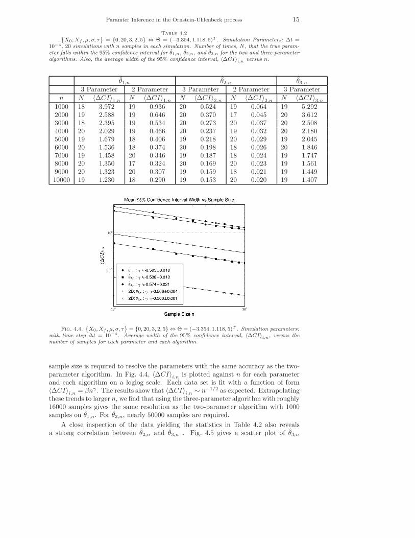
= {0, 20, 3, 2, 5} ⇔ Θ = (−3.354, 1.118, 5)T . Simulation Parameters; ∆t =10−4, 20 simulations with n samples in each simulation. Number of times, N , that the true param-eter falls within the 95% confidence interval for θ̂1,n, θ̂2,n, and θ̂3,n for the two and three parameteralgorithms. Also, the average width of the 95% confidence interval, 〈∆CI〉i,n versus n.

θ̂1,n θ̂2,n θ̂3,n

3 Parameter 2 Parameter 3 Parameter 2 Parameter 3 Parametern N 〈∆CI〉1,n N 〈∆CI〉1,n N 〈∆CI〉2,n N 〈∆CI〉2,n N 〈∆CI〉3,n

1000 18 3.972 19 0.936 20 0.524 19 0.064 19 5.2922000 19 2.588 19 0.646 20 0.370 17 0.045 20 3.6123000 18 2.395 19 0.534 20 0.273 20 0.037 20 2.5084000 20 2.029 19 0.466 20 0.237 19 0.032 20 2.1805000 19 1.679 18 0.406 19 0.218 20 0.029 19 2.0456000 20 1.536 18 0.374 20 0.198 18 0.026 20 1.8467000 19 1.458 20 0.346 19 0.187 18 0.024 19 1.7478000 20 1.350 17 0.324 20 0.169 20 0.023 19 1.5619000 20 1.323 20 0.307 19 0.159 18 0.021 19 1.44910000 19 1.230 18 0.290 19 0.153 20 0.020 19 1.407

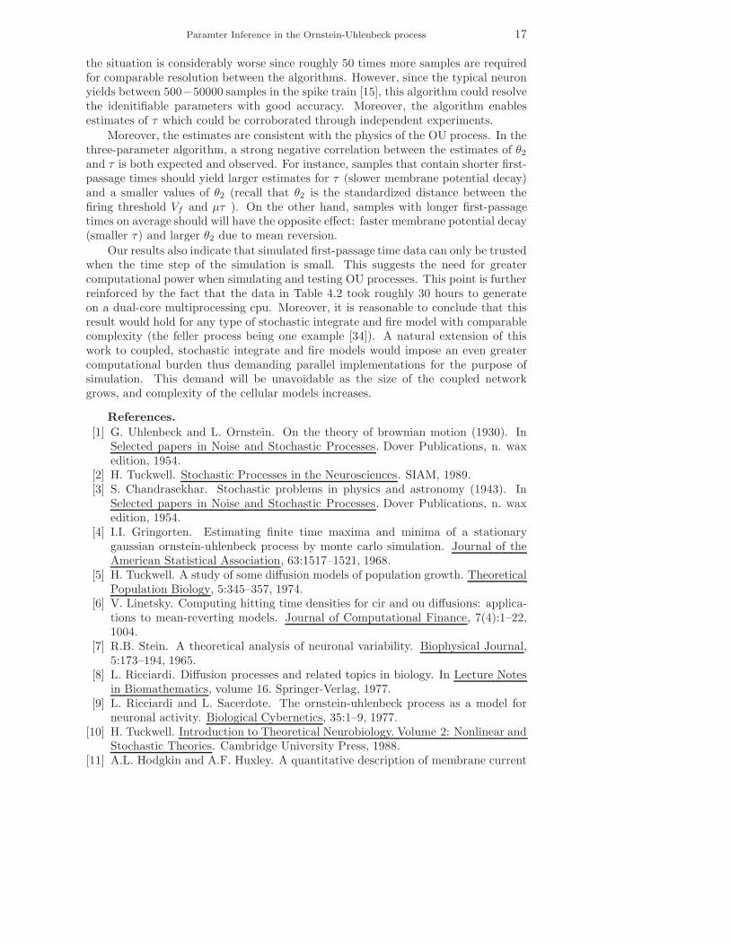
Fig. 4.4.˘

X0, Xf , µ, σ, τ¯

= {0, 20, 3, 2, 5} ⇔ Θ = (−3.354, 1.118, 5)T . Simulation parameters:with time step ∆t = 10−4. Average width of the 95% confidence interval, 〈∆CI〉i,n, versus thenumber of samples for each parameter and each algorithm.

sample size is required to resolve the parameters with the same accuracy as the two-parameter algorithm. In Fig. 4.4, 〈∆CI〉i,n is plotted against n for each parameterand each algorithm on a loglog scale. Each data set is fit with a function of form〈∆CI〉i,n = βnγ . The results show that 〈∆CI〉i,n ∼ n−1/2 as expected. Extrapolatingthese trends to larger n, we find that using the three-parameter algorithm with roughly16000 samples gives the same resolution as the two-parameter algorithm with 1000samples on θ̂1,n. For θ̂2,n, nearly 50000 samples are required.

A close inspection of the data yielding the statistics in Table 4.2 also revealsa strong correlation between θ̂2,n and θ̂3,n . Fig. 4.5 gives a scatter plot of θ̂3,n


Fig. 4.5.˘

X0, Xf , µ, σ, τ¯

= {0, 20, 3, 2, 5} ⇔ Θ = (−3.354, 1.118, 5)T . Simulation parameters:

∆t = 10−4. θ̂3,n versus θ̂2,n for all sample sizes and simulations in Table 4.2. The true value of Θ(i.e. the simulation parameters) is given by the red dot.

versus θ̂2,n for every simulation in every sample size n. A marker denoting the trueparameter value used for the simulation is given for reference. These results are notat all surprising considering the physics of the OU process, although the strength ofthe correlation is surprising. To see this, imagine two distinct OU processes labeledA and B that are subject to the same input drift µ and variance σ. Moreover, letthem have the same resting and firing thresholds X0 and Xf . Lastly, let A have alarger time constant, θ3. Since A has a larger time constant, the state variable of A,XA(t), will decay more slowly than XB(t) and thus can be expected to have shorterfirst-passage times. Shorter first passage-times implies a smaller value of θ2 due tomean-reversion. The same argument can be applied in reverse thus explaining thestrong negative correlation between these parameters.

Although a variety of additional parameter studies could be performed at thisjuncture, we believe that the main differences between the two and three-parameteralgorithms have been demonstrated. Moreover, since the results are typical for anyset of parameters, Θ, the conclusions are completely general.

5. Discussion. We have given an algorithm for computing maximum likelihoodestimates (MLEs) for the three identifiable parameters of the Ornstein-Uhlenbeckprocess. Previous efforts [15, 24, 34] have focused on the two-parameter case wherethe time constant τ is known a priori. When this assumption is introduced intoour algorithm, the resulting parameter estimates and their corresponding confidenceintervals and regions are consistent with theoretical predictions.

However, when only first-passage time data is available, a priori assumptions on τcannot be made and thus the full three-parameter estimation is necessary. Our resultsshow unequivocably that the addition of the τ parameter in the estimation proceduredramatically decreases the resolution of θ1,2 for a fixed sample size. Here, a decrease inresolution corresponds to an increase in the width of the parameters’ 95% confidenceintervals. In fact, case studies have shown that roughly 15 times more samples arerequired to resolve θ1 to the same accuracy as the two-parameter algorithm. For θ2 ,


the situation is considerably worse since roughly 50 times more samples are requiredfor comparable resolution between the algorithms. However, since the typical neuronyields between 500−50000 samples in the spike train [15], this algorithm could resolvethe idenitifiable parameters with good accuracy. Moreover, the algorithm enablesestimates of τ which could be corroborated through independent experiments.

Moreover, the estimates are consistent with the physics of the OU process. In thethree-parameter algorithm, a strong negative correlation between the estimates of θ2

and τ is both expected and observed. For instance, samples that contain shorter first-passage times should yield larger estimates for τ (slower membrane potential decay)and a smaller values of θ2 (recall that θ2 is the standardized distance between thefiring threshold Vf and µτ ). On the other hand, samples with longer first-passagetimes on average should will have the opposite effect: faster membrane potential decay(smaller τ) and larger θ2 due to mean reversion.

Our results also indicate that simulated first-passage time data can only be trustedwhen the time step of the simulation is small. This suggests the need for greatercomputational power when simulating and testing OU processes. This point is furtherreinforced by the fact that the data in Table 4.2 took roughly 30 hours to generateon a dual-core multiprocessing cpu. Moreover, it is reasonable to conclude that thisresult would hold for any type of stochastic integrate and fire model with comparablecomplexity (the feller process being one example [34]). A natural extension of thiswork to coupled, stochastic integrate and fire models would impose an even greatercomputational burden thus demanding parallel implementations for the purpose ofsimulation. This demand will be unavoidable as the size of the coupled networkgrows, and complexity of the cellular models increases.

References.

[1] G. Uhlenbeck and L. Ornstein. On the theory of brownian motion (1930). InSelected papers in Noise and Stochastic Processes. Dover Publications, n. waxedition, 1954.

[2] H. Tuckwell. Stochastic Processes in the Neurosciences. SIAM, 1989.[3] S. Chandrasekhar. Stochastic problems in physics and astronomy (1943). In

Selected papers in Noise and Stochastic Processes. Dover Publications, n. waxedition, 1954.

[4] I.I. Gringorten. Estimating finite time maxima and minima of a stationarygaussian ornstein-uhlenbeck process by monte carlo simulation. Journal of theAmerican Statistical Association, 63:1517–1521, 1968.

[5] H. Tuckwell. A study of some diffusion models of population growth. TheoreticalPopulation Biology, 5:345–357, 1974.

[6] V. Linetsky. Computing hitting time densities for cir and ou diffusions: applica-tions to mean-reverting models. Journal of Computational Finance, 7(4):1–22,1004.

[7] R.B. Stein. A theoretical analysis of neuronal variability. Biophysical Journal,5:173–194, 1965.

[8] L. Ricciardi. Diffusion processes and related topics in biology. In Lecture Notesin Biomathematics, volume 16. Springer-Verlag, 1977.

[9] L. Ricciardi and L. Sacerdote. The ornstein-uhlenbeck process as a model forneuronal activity. Biological Cybernetics, 35:1–9, 1977.

[10] H. Tuckwell. Introduction to Theoretical Neurobiology. Volume 2: Nonlinear andStochastic Theories. Cambridge University Press, 1988.

[11] A.L. Hodgkin and A.F. Huxley. A quantitative description of membrane current


and its application to conduction and excitation in nerves. Journal of Physiology,117:500–544, 1952.

[12] R. Chhikara and J.L. Folks. The Inverse Gaussian Distribution: Theory,Methodology, and Applications. Marcel-Dekker, 1988.

[13] B. Jorgensen. The Generalized Inverse Gaussian Distribution. Springer, 1981.[14] S. Iyengar and Q. Liao. Modeling neural activity using the generalized inverse

gaussian distribution. Biological Cybernetics, 77:289–295, 1997.[15] L. Ricciardi and S. Sato. First passage time density and moments of the ornstein-

uhlenbeck process. J. of Applied Probability, 25:43–57, 1988.[16] L. Arnold. Stochastic Differential Equations: Theory and Applications. John

Wiley and Sons, 1974.[17] S. Karlin and H. Taylor. A Second Course in Stochastic Processes. Academic

Press, 1981.[18] D. Darling and A. Siegert. The first passage problem for a continuous markov

process. Annals of Mathematical Statistics, 24:624–639, 1953.[19] A.J.F. Siegert. On the first passage time probablity functioin. Physical Review,

81:617–623, 1951.[20] N.N. Lebedev. Special Functions and their Applications. Dover Publications,

1972.[21] R.V. Churchill. Operational Mathematics. McGraw-Hill, 1981.[22] E.L. Lehmann. Theory of Point Estimation. John Wiley and Sons, 1983.[23] S. Iyengar and P. Mullowney. Parameter estimation in the ornstein-uhlenbeck

process. Submitted to: submitted to The Annals of Statistics, 2006.[24] J. Inoue, S. Sato, and L. Ricciardi. On the parameter estimation for diffusion

models of single neuron’s activities. Biological Cybernetics, 73:209–221, 1995.[25] W.T. Weeks. Numerical inversion of the laplace transform using laguerre func-

tions. Journal of Association of Computational Mathematics, 13:419–429, 1966.[26] P.O. Kano, B. Moysey, and J.V. Moloney. Application of weeks method for

the numerical inversion of the laplace transform of the matrix exponential.Computational Mathematical Sciences, 3:335–372, 2005.

[27] F.R. De Hoog, J.H. Knight, and A.N. Stokes. An improved method for numer-ical inversion of laplace transforms. SIAM Journal of Scientific and StatisticalComputing, 3:357–366, 1982.

[28] L. D’Amore, G. Laccetti, and A. Murli. An implementation of a fourier seriesmethod for the numerical inversion of the laplace transform. ACM Transactionson Mathematical Software, 25:279–305, 1999.

[29] C. G. Broyden. A class of methods for solving nonlinear simultaneous equations.Mathematical Computing, 19:577–593, 1965.

[30] M. Abramowitz and I.R. Stegun. Handbook of Mathematical Functions. DoverPublications Inc, 9 edition, 1972.

[31] J.C.P Miller. National Physical Laboratory, Tables of Weber parabolic cylinderfunctions. Her Majesty’s Stationary Office, 1955.

[32] C.M. Bender and S.A. Orzag. Advanced mathematical methods for scientistsand Engineers. McGraw Hill, 1978.

[33] M.A. Stephens. Edf statistics for goodness of fit and some comparisons. Journalof the American Statistical Association, 69:730–737, 1974.

[34] S. Ditlevsen and O. Ditlevsen. Parameter estimation from observations of first-passage times of the ornstein-uhlenbeck process and the feller process. Presentedat the Fifth Computational Stochastic Mechanics Conference, 2006.

maximum likelihood estimation and computation for the ornstein-uhlenbeck process

Documents