Thesis for the degree of Master of Science

Generalized Ornstein-Uhlenbeckprocesses

Vladyslav Bezuglyy

Department of Physics and Engineering PhysicsChalmers University of Technology

Goteborg, Sweden 2006

Generalized Ornstein-Uhlenbeck processes

Vladyslav Bezuglyy

c© Vladyslav Bezuglyy, 2006

Department of Physics and Engineering PhysicsChalmers University of TechnologySE–412 96 GoteborgSwedenTelephone: +46 (0)31–772 1000

Abstract

This thesis discusses diffusive motion of particles experiencing random forc-ing in a viscous medium. It generalizes the standard Ornstein-Uhlenbeckprocess in one spatial dimension (which is also discussed) for the case whenthe dependence of the force on the position of the particle cannot be ne-glected. Expectation values and correlation functions of physical observables(momentum and displacement) are calculated. This is achieved by findingthe spectrum of the so-called Fokker-Planck operator describing the timeevolution of the probability distribution of momentum. Numerical experi-ments are performed confirming the analytical results obtained. The caseof two spatial dimensions is briefly discussed and numerical results for thiscase are presented.

Contents

1 Introduction 5

2 The model 72.1 Random-field generation . . . . . . . . . . . . . . . . . . . . . 8

2.1.1 Spectral decomposition of a random function . . . . . 82.1.2 Synthetic turbulence . . . . . . . . . . . . . . . . . . . 92.1.3 Time correlation function . . . . . . . . . . . . . . . . 10

3 The standard Ornstein-Uhlenbeck process 12

4 Spectral decomposition of the Fokker-Planck operator of thegeneralized Ornstein-Uhlenbeck process 154.1 Eigenvalues and eigenfunctions . . . . . . . . . . . . . . . . . 174.2 Correlation functions . . . . . . . . . . . . . . . . . . . . . . . 19

4.2.1 Matrix elements Y0n . . . . . . . . . . . . . . . . . . . 194.2.2 Matrix elements Zmn . . . . . . . . . . . . . . . . . . . 204.2.3 Ratio of the eigenfunctions . . . . . . . . . . . . . . . 22

5 Results 245.1 Momentum equilibrium correlation function . . . . . . . . . . 245.2 Momentum diffusion . . . . . . . . . . . . . . . . . . . . . . . 255.3 Spatial diffusion . . . . . . . . . . . . . . . . . . . . . . . . . 26

5.3.1 Long-time diffusion . . . . . . . . . . . . . . . . . . . . 265.3.2 Short-time anomalous diffusion . . . . . . . . . . . . . 28

6 Motion in two spatial dimensions 32

7 Conclusions and future work 35

4

Chapter 1

Introduction

This thesis addresses the problem of describing the dynamics of particlesmoving in a viscous medium. This problems has recently been intensivelyinvestigated. Examples are passive tracers in turbulent flows [1] and inertialparticles in turbulent flows [2, 3, 4, 5]. Early works go back to Einstein[6] and Smoluchowski [7] in the theory of Brownian motion showing amongother results diffusive motion of particles. Subsequently Ornstein and Uh-lenbeck [8] considered the equation of motion of a particle of mass m,

mdu

dt= −ku + f(t). (1.1)

Here, f(t) represents a randomly fluctuating force, u is the velocity of theparticle and k is the friction coefficient. Ornstein and Uhlenbeck obtainedresults for the mean square values of the displacement of the particle, 〈x2(t)〉,and the velocity 〈u2(t)〉, as well as the probability distribution of the velocity.

In this thesis this problem is generalized by considering the equation ofmotion,

mdu

dt= −ku + f(x, t), (1.2)

where the force f(x, t) depends not only on time, but also on the positionof a particle (as is generally the case).

Properties of particles moving according to (1.2) have been studied in-tensively in the past. In particular, the evolution of distribution of manyparticles moving in a turbulent flow that can be approximated by (1.2) isof major interest. Surprisingly, for non-interacting particles, it appearedthat (1.2) exhibits a phase transition between two regimes: in the first oneparticles seem to move completely independently as one might expect fordiffusive motion; in the second one particles tend to cluster together and, inthe end, explore the same trajectory. Deutsch [9] described this phenomenonand gave theoretical statements and numerical simulations showing an ex-istence of a phase transition. In [10, 11] the Lyapunov exponent - the rate

5

of exponential convergence (divergence) of nearby trajectories - was explic-itly calculated as a function of a dimensionless parameter characterizing themodel (1.2) both for one-dimensional and two-dimensional cases. The Lya-punov exponent for the three-dimensional case was calculated in [5] and [12],which is most important for physical applications. Sigurgeirsson and Stuart[16] investigated model (1.2) incorporating collisions between particles.

The aim of this thesis is to calculate the mean square values of themomentum and the displacement, 〈p2(t)〉, 〈x2(t)〉 respectively, as well asthe correlation function of the momentum 〈p(t)p(t+∆t)〉 in equilibrium forparticles moving according to (1.2). This is achieved by finding a spectrumof the corresponding operator of the Fokker-Planck equation that describesthe evolution of the probability distribution of momentum. The spectrum isused to write the propagator that defines correlation functions. This is doneassuming motion in the limit of small damping and large forcing. This makesit possible to simplify the Fokker-Planck equation. This problem has beeninvestigated in [15], and the results obtained there are generalized. Thereare also asymptotic scaling results available in [13] and [14] for the case ofundamped motion (k = 0), for an arbitrary dimension both for classical andquantum particles.

This report is organized in the following way. The second chapter de-scribes the model and introduces all parameters. It also describes themethod used for the numerical simulation of random force field f(x, t).Chapter 3 is dedicated to the standard Ornstein-Uhlenbeck process. Chap-ter 4 introduces the Fokker-Planck equation for model (1.2) and the cor-responding operator, its spectral decomposition, and correlation functionsthat can be determined using eigenvalues and eigenfunctions. Chapter 5presents the results for momentum and spatial diffusion for the generalizedOrnstein-Uhlenbeck process compared with numerical results. Chapter 6gives a brief discussion for the case of two spatial dimensions. Conclusionsare summarized in chapter 7.

6

Chapter 2

The model

Consider a particle with mass m, position x and momentum p moving in anone-dimensional random force field f(x, t) characterized by damping rate γ.The equation of motion is

dx

dt=

p

m, (2.1)

dp

dt= −γp + f(x, t).

Note that the original Ornstein-Uhlenbeck equation (1.1) is written in termsof a friction coefficient k. It is related to γ as follows: k = γm.

The following assumptions concerning f(x, t) are made. First, the meanvalue of the force f(x, t) over an ensemble of realizations for any x and t isassumed to vanish, that is,

〈f(x, t)〉 = 0. (2.2)

Angular brackets denote the mean value throughout the report.Furthermore, it is assumed that correlations between values of f(x, t) for

different x1, t1 and x2, t2 decay fast with increasing |x2 − x1| and |t2 − t1|with scaling factors, ξ and τ respectively. The correlation function of theforce can be written as follows,

〈f(x1, t1)f(x2, t2)〉 = c(x1 − x2, t1 − t2). (2.3)

In the numerical simulations, the following form of the correlation functionis used,

c(x, t) = 〈f(x1, t1)f(x1 + x, t1 + t)〉 (2.4)

= σ2exp(− x2

2ξ2

)exp

(−|t|

τ

),

7

where σ is the typical strength of the force. A random field having suchproperties is referred as a generic random field and, accordingly, this case iscalled the generic case. Another possibility is to generate a force field as

f(x, t) =∂ψ(x, t)

∂x, (2.5)

where ψ(x, t) is a generic random field as described above. This case isreferred as the gradient case. Note that for this case the typical strengthof the force is σ/ξ. Later it will be shown how the form of the correlationfunction for the gradient case can be calculated.

2.1 Random-field generation

Numerical methods for creating random fields are usually based on spec-tral or Fourier decomposition of a random function similar to the case of anon-random function. In order to verify the analytical results discussed inchapter 5, it is important to have a method for simulating the random forcein (1.2) that is fast and memory efficient.

2.1.1 Spectral decomposition of a random function

Here, spectral decomposition of a random function of one variable is brieflydescribed. It is assumed that

〈f(x)〉 = 0, (2.6)〈f(x1)f(x1 + x)〉 = c(x).

An extension to the case of more than one variable is straightforward.The spectral decomposition of a periodic random function f(x) with a

period L looks as follows,

f(x) =∑

k∈Kfk exp(ikx), (2.7)

where K is the set of the form 2πL n and n = 0,±1,±2, . . . The coefficients

fk are complex numbers, but in order for f(x) to be real one has to choosef0 to be a real number and f−k = f∗k , where the asterisk denotes complex-conjugation. The fk’s are chosen to be independent random numbers withparticular properties, and from the first condition of (2.6) it clearly followsthat 〈fk〉 = 0. The second condition implies that the variance of any fk mustbe equal to the value of a required spectral density s(k), which is, simply,the Fourier transform of a correlation function,

s(k) =1L

∫ ∞

−∞c(x)exp (ikx) dx, (2.8)

c(x) =L

2π

∫ ∞

−∞s(k)exp (ikx) dk.

8

This implies that the variance of f(x) is equal to the sum of variances of allfk’s, that is,

〈f2(x)〉 = c(0) =∑

k∈K〈|fk|2〉. (2.9)

These statements might be enough to start generating a random func-tion. However, computational problems arises. The time necessary for com-puting the sum (2.7) grows quickly with a number of terms N and thedimension d, namely as Nd, that is exponentially with the dimension. Notealso that upon increasing the period L, one has to increase the number ofterms to reliably approximate the indefinite sum (2.7). If a random fielddepends on discrete variables it is possible to apply fast Fourier transforms(FFT) to compute (2.7). This might be useful for the present problem. FFTis a very powerful technique that makes it possible to reduce the growth ofthe computing time from Nd to Nd−n log Nn, where n is the number of dis-crete variables, but it can be crucially exacting for memory resources, if thenumber of discrete steps is very large (and this is the case).

Sigurgeirsson and Stuart [16] described a method for generating a spatialrandom field evolving in time that is also based on spectral decomposition.They showed that it is possible to use a differential equation to generatefk(t) to simulate the desired time correlation function while at a given timet the coefficients fk(t) determine the desired spatial correlation function.Sigurgeirsson et al. [17] referred to this approach as synthetic turbulence.

2.1.2 Synthetic turbulence

This section describes how a random field of two variables (one in space andone in time) can be generated. The algorithm presented in [16] is adoptedwith some modifications. The idea is to use spectral decomposition of theform (2.7),

f(x, t) =∑

k∈Kfk(t)exp(ikx). (2.10)

The distribution of fk must remain stationary and satisfy the constraint〈|fk(t)|2〉 = s(k), where s(k) is the Fourier transform of the spatial correla-tion function. Using the correlation function of the form (2.4) the requiredspectral density is

s(k) =√

2πσ2ξ

Lexp

(−ξ2k2

2

). (2.11)

In order to reproduce the desired time correlation function, fk(t) can begenerated dynamically using a differential equation. It can be easily verifiedthat in order to get the time correlation function of the form (2.4) fk(t)must be solutions of the following differential equation,

dfk

dt= −τ−1fk +

√2s(k)

τ

dβk

dt, (2.12)

9

where βk is a sequence of standard complex-valued Brownian motions, i.e.〈dβk(t)〉 = 0, and 〈dβk(t1)dβ∗k(t2)〉 = δt1t2dt. In order for f(x, t) to be realone has to choose βk = β∗−k, fk = f∗−k and f0 to be a real number. At t = 0,the fk’s must be chosen from a normal distribution N [0, s(k)], which is astationary distribution of (2.12).

Unfortunately, there are not many types of correlation functions thatcan be simulated by this method, and it is not obvious how to constructa differential equation for a given correlation function, whereas for FFT itis necessary to know only a spectral density. The method based on (2.10)and (2.12) is much faster than the one described in section 2.1.1, and it istherefore used to simulate the random force in (2.1).

2.1.3 Time correlation function

It is now possible to calculate the correlation function of the force for thegradient case by writing a spatial derivative of (2.10) as follows,

g(x, t) =∂f(x, t)

∂x= i

∑

k∈Kkfk(t)exp(ikx). (2.13)

The unique solution of (2.12) (assuming t > 0) is

fk(t) = fk(0)exp(− t

τ

)+

√2s(k)

τ

∫ t

0exp

(z − t

τ

)dβk(z). (2.14)

The time correlation function can be calculated by averaging g(0, 0)g(0, t)over an ensemble of realizations,

c(t) = 〈g(0, 0)g(0, t)〉 =∑

k∈K〈k2fk(0)fk(t)〉. (2.15)

Using (2.14) this can be rewritten as follows,

c(t) =∑

k∈Kk2〈f2

k (0)〉exp(− t

τ

)(2.16)

+∑

k∈K

√2s(k)

τ

⟨∫ t

0exp

(z − t

τ

)dβk(z)

⟩. (2.17)

The average value of the term with the integral is 0, since dβk are indepen-dent increments in time. Therefore,

c(t) =∑

k∈Kk2〈fk(0)2〉exp

(− t

τ

)(2.18)

=∑

k∈Kk2s(k)exp

(− t

τ

)=

σ2

ξ2exp

(− t

τ

).

10

The spatial correlation function c(x) is determined as follows,

c(x) = 〈g(0, 0)g(x, 0)〉. (2.19)

Using (2.13) this yields,

c(x) =∑

k∈Kk2s(k)exp(ikx) =

σ2(ξ2 − x2)ξ4

exp(− x2

2ξ2

). (2.20)

Summarizing, the correlation function for the gradient case is

c(x, t) =σ2

ξ4(ξ2 − x2)exp

(− x2

2ξ2

)exp

(−|t|

τ

). (2.21)

Henceforth c(x, t) is referred as the correlation function and c(x) and c(t)are referred as its spatial and time part respectively.

11

Chapter 3

The standardOrnstein-Uhlenbeck process

This chapter describes the standard Ornstein-Uhlenbeck process. The ma-terial in this chapter is taken from [8] (see also [19]).

The equation of motion considered by Ornstein and Uhlenbeck (in termsof damping rate γ) is

dp

dt= −γp + f(t). (3.1)

Let f(t) have the following properties:

〈f(t)〉 = 0, (3.2)〈f(t1)f(t1 + t)〉 = c(t),

where c(t) is a function with a sharp maximum at t = 0 with correlationlength τ [e.g. the time part of the correlation function of the form (2.4)]. Thesolution of (3.1), that is, the dynamics of the momentum can be calculatedby integrating the differential equation (assuming initial condition p(0) = 0),

p(t) = e−γt

∫ t

0eγsf(s)ds. (3.3)

The variance of the momentum is thus

〈p2(t)〉 = e−2γt

∫ t

0ds1

∫ t

0ds2eγ(s1+s2)〈f(s1)f(s2)〉. (3.4)

By changing the variables s1 + s2 = u, s1 − s2 = v, (3.4) becomes

〈p2(t)〉 =12e−2γt

∫ 2t

0eγudu

∫ t

−tc(v)dv. (3.5)

Since c(v) has a sharp maximum at v = 0, it is possible to change the limitsof integration of the second integral in (3.5) to (−∞;∞) for t À τ to obtain

〈p2(t)〉 =D0

γ(1− e−2γt) (3.6)

12

with the diffusion constant

D0 =12

∫ ∞

−∞c(t)dt. (3.7)

The variance of the displacement is obtained by integrating (3.3) (assumingfor the sake of simplicity x(0) = 0),

x(t) =1m

∫ t

0e−γudu

∫ u

0eγvf(v)dv, (3.8)

or integrating by parts,

x(t) =1

γm

(∫ t

0f(u)du− e−γt

∫ t

0eγuf(u)du

). (3.9)

By squaring and averaging the variance of the displacement becomes,

〈x2(t)〉 =1

γ2m2

∫ t

0du

∫ t

0dv 〈f(u)f(v)〉 (3.10)

− 2e−γt

γ2m2

∫ t

0du

∫ t

0dv eγu〈f(u)f(v)〉

+e−2γt

γ2m2

∫ t

0du

∫ t

0dv eγ(u+v)〈f(u)f(v)〉.

It is convenient to change variables in the first and the third terms as a =u + v and b = u− v, whereas for the second term the change of variables isa = u and b = u− v. This gives the following result,

〈x2(t)〉 =1

2γ2m2

∫ 2t

0da

∫ t

−tdb c(b) (3.11)

− 2e−γt

γ2m2

∫ t

0da eγa

∫ t

−tdb c(b)

+e−2γt

2γ2m2

∫ 2t

0da eγa

∫ t

−tdb c(b).

As before, it is possible to approximate the second integral in all 3 terms as2D0 for t À τ obtaining

〈x(t)2〉 =2D0

γ2m2

[t +

1− e−2γt

2γ− 2(1− e−γt)

γ

]. (3.12)

The last expression implies anomalous diffusion at short times,

〈x(t)2〉 ∼ 2D0

3m2t3 (3.13)

13

10-3 10-2 10-1 100 10110-4

10-3

10-2

10-1

100

10-3 10-2 10-1 100 101 10210-11

10-9

10-7

10-5

10-3

10-1

101

103

<p2 (t

)>D

0-1

t

<x2 (t

)> D

0-1m

23

t

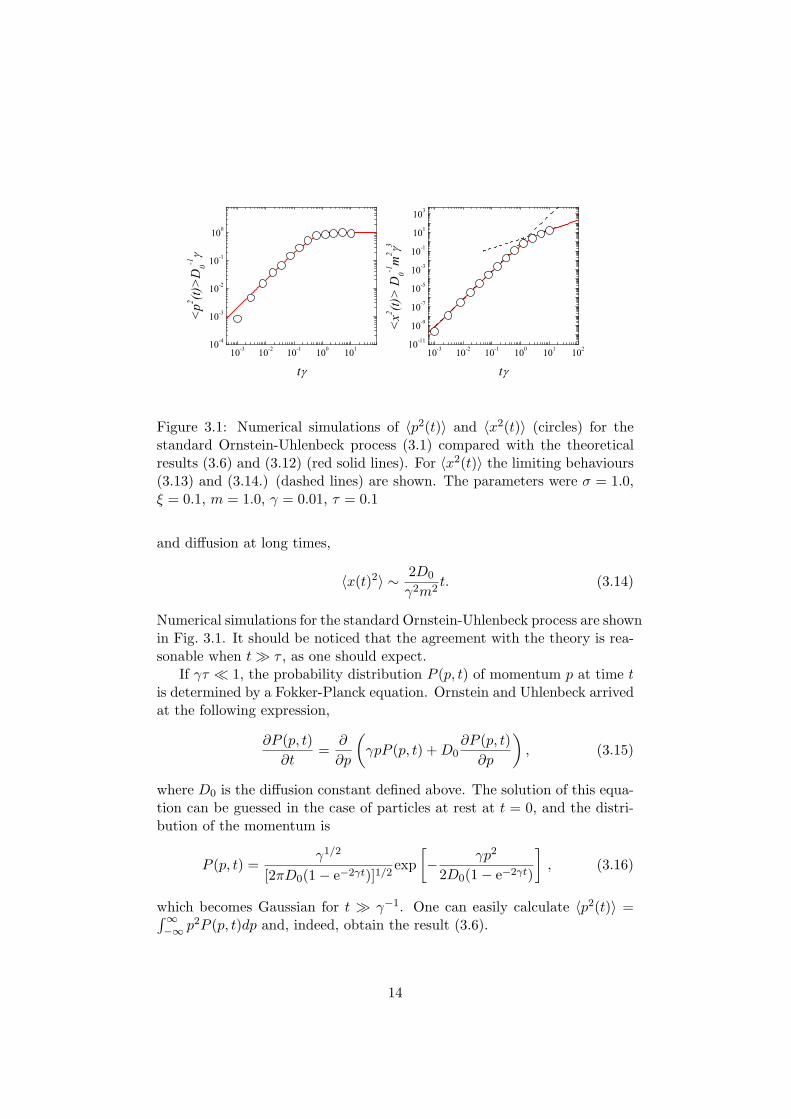
Figure 3.1: Numerical simulations of 〈p2(t)〉 and 〈x2(t)〉 (circles) for thestandard Ornstein-Uhlenbeck process (3.1) compared with the theoreticalresults (3.6) and (3.12) (red solid lines). For 〈x2(t)〉 the limiting behaviours(3.13) and (3.14.) (dashed lines) are shown. The parameters were σ = 1.0,ξ = 0.1, m = 1.0, γ = 0.01, τ = 0.1

and diffusion at long times,

〈x(t)2〉 ∼ 2D0

γ2m2t. (3.14)

Numerical simulations for the standard Ornstein-Uhlenbeck process are shownin Fig. 3.1. It should be noticed that the agreement with the theory is rea-sonable when t À τ , as one should expect.

If γτ ¿ 1, the probability distribution P (p, t) of momentum p at time tis determined by a Fokker-Planck equation. Ornstein and Uhlenbeck arrivedat the following expression,

∂P (p, t)∂t

=∂

∂p

(γpP (p, t) + D0

∂P (p, t)∂p

), (3.15)

where D0 is the diffusion constant defined above. The solution of this equa-tion can be guessed in the case of particles at rest at t = 0, and the distri-bution of the momentum is

P (p, t) =γ1/2

[2πD0(1− e−2γt)]1/2exp

[− γp2

2D0(1− e−2γt)

], (3.16)

which becomes Gaussian for t À γ−1. One can easily calculate 〈p2(t)〉 =∫∞−∞ p2P (p, t)dp and, indeed, obtain the result (3.6).

14

Chapter 4

Spectral decomposition ofthe Fokker-Planck operatorof the generalizedOrnstein-Uhlenbeck process

This chapter discusses the spectral decomposition of the Fokker-Planck oper-ator corresponding to (2.1) in the limit of small damping. The Fokker-Planckequation in this case looks as follows [13, 14, 15, 18],

∂P (p, t)∂t

=∂

∂p

(γpP (p, t) + D(p)

∂P (p, t)∂p

), (4.1)

with a diffusion constant that now depends on p,

D(p) =12

∫ ∞

−∞c(pt/m, t) dt. (4.2)

The limits of validity of (4.1) are discussed in [22]. If damping rate γ is smalland the force is large particles travel very fast compared with the typicalmomentum of the model p0 = mξ/τ and the diffusion constant D(p) can beapproximated in the limit of p À p0.

First, D(p) is calculated for the generic case using the correlation func-tion of the form (2.4),

D(p) =mσ2ξexp

(m2ξ2

2p2τ2

)erfc

(mξ

|p|τ√2

)√π

|p|√2, (4.3)

where erfc(x) is the complementary error function [20]. By denoting D1 =σ2τ one has,

D(p) = D1p0

|p|exp(

p20

2p2

)erfc

(p0

|p|√2

). (4.4)

15

Assuming p À p0 it is possible to keep only the terms p0/p of first orderand obtain,

D(p) ∼ D1p0

|p| . (4.5)

Now, D(p) for the gradient case can be calculated using the correlationfunction of the form (2.21),

D(p) =m2σ2

[2|p|τ −mξexp

(m2ξ2

2p2τ2

)erfc

(mξ

pτ√

2

)√2π

]

2|p|3τ2(4.6)

and denoting D2 = σ2τ/ξ2 one obtains,

D(p) = D2p20

p2−D2

p30

|p|3 exp(

p20

2p2

)erfc

(p0

|p|√2

)√π

2. (4.7)

Assuming p À p0 it is possible to keep only the terms p0/p of second orderand obtain,

D(p) ∼ D2

(p0

p

)2

. (4.8)

It is argued [15] that for any differentiable force (e.g. time correlation func-tion of the Gaussian form) one obtains either D(p) ∼ p−1 (the generic case)or D(p) ∼ p−3 (the gradient case). Indeed, the correlation function (2.4) isnot differentiable at t = 0. This gives rise to D(p) ∼ p−2 for the gradientcase. To generalize, one may assume that the diffusion constant behaves as

D(p) = Dζ

∣∣∣∣p0

p

∣∣∣∣ζ

. (4.9)

Values of ζ different from 1,2 or 3 arise for correlation functions of algebraicform.

The Fokker-Planck equation for the generic case with the diffusion con-stant approximated for large p looks as follows,

∂P

∂t=

∂

∂p

(γpP + D1

p0

|p|∂P

∂p

). (4.10)

Assuming that at t = 0 all particles are at rest initial condition is P (p, 0) =δ(p). The solution of (4.10) can be guessed then,

P (p, t) =1

2Γ(4/3)γ1/3

[3p0D1(1− e−3γt)]1/3exp

[− γ|p|3

3p0D1(1− e−3γt)

]. (4.11)

Using this probability distribution it is possible to calculate the variance ofthe momentum,

〈p2(t)〉 =∫ ∞

−∞p2P (p, t)dp =

(p0D1

γ

)2/3 131/3Γ(4/3)

(1− e−3γt)2/3. (4.12)

16

This reproduces the result obtained in [15].Similarly for the gradient case one obtains the Fokker-Planck equation

with the approximated diffusion constant,

∂P

∂t=

∂

∂p

(γpP + D2

(p0

p

)2 ∂P

∂p

). (4.13)

The probability distribution function for the gradient case is,

P (p, t) =1

2Γ(5/4)γ1/4

[4p20D2(1− e−4γt)]1/4

exp[− γp4

4p20D2(1− e−4γt)

](4.14)

and the variance of the momentum,

〈p2(t)〉 =(

p20D2

γ

)1/2 2Γ(3/4)Γ(1/4)

(1− e−4γt)1/2. (4.15)

4.1 Eigenvalues and eigenfunctions

It has been shown above how the probability distribution of momentumcan be obtained using the Fokker-Planck equation. However, the generalsolution for arbitrary initial condition is not found in closed form. Therefore,the following approach is adopted.

It is assumed that the diffusion constant is of the form (4.9) for large p.First, it is convenient to introduce dimensionless variables,

t′ = γt, z = pγ

12+ζ

pζ

2+ζ

0 D1

2+ζ

ζ

. (4.16)

Then the Fokker-Planck equation (4.1) becomes

∂P (z, t′)∂t′

=∂

∂z

(zP (z, t′) +

1|z|ζ

∂P (z, t′)∂z

)≡ FP, (4.17)

which defines the Fokker-Planck operator F . The stationary distribution ofthis equation is P0(z) ∝ exp[−|z|ζ+2/(ζ + 2)]. Therefore, one can write theHermitian form of the operator F ,

H = P−1/20 FP

1/20 =

12− |z|2+ζ

4+

∂

∂z

1|z|ζ

∂

∂z, (4.18)

which is sometimes referred as the Hamiltonian operator. To begin with,an eigenvalue of H os λ+

0 = 0, and the corresponding eigenfunction is

ψ+0 = C+

0 exp(− |z|2+ζ

4+2ζ

). It turns out that λ+

0 is the lowest eigenvalue. Thenext eigenvalue can be determined by inspection as well (e.g. by putting ζ

17

to any particular value and generalizing). It is λ−0 = −1− ζ and the corre-

sponding eigenfunction is ψ−0 = C−0 z|z|ζexp(− |z|2+ζ

4+2ζ

). The eigenfunctions

and eigenvalues are labeled by superscripts ’+’ and ’-’ to emphasize thateigenfunctions ψ+

n are even functions and ψ−n are odd functions.Now, the following operators are introduced,

a± =∂

∂z± z|z|−ζ

2, (4.19)

A = a+|z|−ζ a+, A+ = a−|z|−ζ a−,

G = a+|z|−ζ a−.

In terms of a+ and a− it can be derived that H = a−|z|−ζ a+. The followingrelations hold,

[H, A] = (2 + ζ)A, [H, A+] = −(2 + ζ)A+, (4.20)

where [X, Y ] = XY − Y X is the commutator. Consider, now

HA+|ψ±n 〉 − A+H|ψ±n 〉 = −(2 + ζ)A+|ψ±n 〉. (4.21)

Here eigenfunctions are written using bra-ket or Dirac notation [23]. Thedefinition of the eigenfunction, namely H|ψ±n 〉 = λn|ψ±n 〉, makes it possibleto write,

A+|ψ±n 〉(λn − 2− ζ) = HA+|ψ±n 〉 (4.22)

This means that A+|ψ±n 〉 is also the eigenfunction of H with the eigenvalueλn − 2− ζ. Together with λ+

0 = 0 and λ−0 = −1− ζ this gives the spectrumof (4.18),

λ+n = −(2 + ζ)n, λ−n = −(2 + ζ)n− 1− ζ. (4.23)

The operators A+ and A thus act as rasing and lowering operators respec-tively:

A+|ψ±n 〉 = C±n+1|ψ±n+1〉, A|ψ±n 〉 = C±

n |ψ±n−1〉. (4.24)

To determine the factors C±n one can use the normalization constraint for

the eigenfunctions,

〈ψ±n+1|ψ±n+1〉 = (C±n+1)

−2〈ψ±n |AA+|ψ±n 〉 = 1. (4.25)

and using the definition of the commutator,

1 = (C±n+1)

−2〈ψ±n |[AA+] + A+A|ψ±n 〉, (4.26)

that is,(C±

n+1)2 = (2 + ζ)(−2λ±n + 1) + (C±

n )2. (4.27)

Recursion gives,

(C±n+1)

2 = (2 + ζ)n∑

k=0

(−2λ±k + 1). (4.28)

Evaluation of the sum yields,

C±n =

√(ζ + 2)n[(ζ + 2)n∓ (ζ + 1)]. (4.29)

18

4.2 Correlation functions

In this correlation functions of the momentum are obtained using the eigen-values and eigenfunction of (4.18. The propagator of the Fokker-Planckequation (4.1) can be written in terms of eigenfunctions as follows [15, 19],

K(y, z; t′) =∞∑

n=0

∑σ=±

P−1/20 (y)ψσ

n(y)P 1/20 (z)ψσ

n(z)exp(λσnt′). (4.30)

The propagator K(y, z, t′) satisfies the Fokker-Planck equation (4.1) andcan be used to compute correlation functions. In order to find 〈p2(t)〉 and〈x2(t)〉 one has to calculate the correlation functions of z2(t′) and z(t′1)z(t′2).For z2(t′) one obtains,

〈z2(t′)〉 =∫ ∞

−∞dz z2K(0, z; t′) =

∞∑

n=0

ψ+n (0)

ψ+0 (0)

〈ψ+0 |z2|ψ+

n 〉exp(λ+n t′). (4.31)

The required correlation function for z(t′1)z(t′2) is

〈z(t′2)z(t′1)〉 =∫ ∞

−∞dz1

∫ ∞

−∞dz2z1z2K(z1, z2; t′2 − t′1)K(0, z1; t1) (4.32)

=∑n,m

ψ+m(0)

ψ+0 (0)

〈ψ+0 |z|ψ−n 〉〈ψ−n |z|ψ+

m〉exp[λ−n (t′2 − t′1) + λ+mt′1].

The terms of the sums (4.31) and (4.32) are calculated in the next threesections, namely matrix elements Y0n = 〈ψ+

0 |z2|ψ+n 〉 and Zmn = 〈ψ+

m|z|ψ−n 〉,as well as the ratio of the eigenfunctions ψ+

m(0)/ψ+0 (0).

4.2.1 Matrix elements Y0n

Consider Y0n = 〈ψ+0 |z2|ψ+

n 〉. Using (4.24) one can obtain Y0n+1 as follows,

Y0n+1 = 〈ψ+0 |z2A+|ψ+

n 〉/C+n+1. (4.33)

It is possible to write zA+ as zG + z(A+ − G) = z(H − I) + z(A+ − G),where I is the identity operator. Using this (4.33) becomes

Y0n+1C+n+1 = 〈ψ+

0 |z2(H − I)|ψ+n 〉+ 〈ψ+

0 |z2(A+ − G)|ψ+n 〉 (4.34)

= (λ+n − 1)Y0n + 〈ψ+

0 |z2(A+ − G)|ψ+n 〉,

and using A+ − G = −za−

Y0n+1C+n+1 = (λ+

n + 2)Y0n. (4.35)

Recursion gives the following,

Y0n = Y00

n∏

k=1

λ+k−1 + 2

C+k

. (4.36)

19

Taking into account that Y00 = (2 + ζ)2

2+ζ Γ( 32+ζ )/Γ( 1

2+ζ ) evaluation of theproduct yields the result,

Y0n = (−1)n(2 + ζ)

22+ζ Γ( 3

2+ζ )Γ(n− 22+ζ )

Γ(− 22+ζ )

√Γ(n + 1)Γ(n + 1

2+a)Γ( 12+a)

. (4.37)

4.2.2 Matrix elements Zmn

Now, consider the matrix elements Zmn = 〈ψ+m|z|ψ−n 〉. It is convenient to

consider first the following element,

Jmn = 〈ψ+0 |Amz(A+)n|ψ−0 〉. (4.38)

The relation between Jmn and Zmn is

Zmn =Jmn

m∏k=1

C+k

n∏k=1

C−k

. (4.39)

For m ≤ n one has,

Jmn = 〈ψ+0 |Am[z, A+](A+)n−1|ψ−0 〉+ 〈ψ+

0 |AmA+z(A+)n−1|ψ−0 〉. (4.40)

The following property

[z, A+] = −(|z|−ζ a− + a−|z|−ζ) (4.41)

makes it possible to write

Jmn = −〈ψ+0 |Am|z|−ζ a−(A+)n−1|ψ−0 〉 − 〈ψ+

0 |Ama−|z|−ζ(A+)n−1|ψ−0 〉(4.42)

+ 〈ψ+0 |AmA+z(A+)n−1|ψ−0 〉 = J (1)

mn + J (2)mn + J (3)

mn.

The third terms evaluates to

J (3)mn = 〈ψ+

0 |AmA+z(A+)n−1|ψ−0 〉 = (C+m)2〈ψ+

0 |Am−1z(A+)n−1|ψ−0 〉 (4.43)

= (C+m)2Jm−1n−1.

Using

Am|z|−ζ a−(A+)n−1 = Am−1a+|z|−ζ a+|z|−ζ a−(A+)n−1 (4.44)

= Am−1a+|z|−ζG(A+)n−1.

it follows that

〈ψ+0 |Am|z|−ζ a−(A+)n−1|ψ−0 〉 = (λ−n−1 − 1) (4.45)

× 〈ψ+0 |Am−1a+|z|−ζ(A+)n−1|ψ−0 〉.

20

Using

Am−1a+|z|−ζ(A+)n−1 = Am−1a+|z|−ζ a−|z|−ζ a−(A+)n−2 (4.46)

= Am−1G|z|−ζ a−(A+)n−2

one obtains the recursion,

J (1)mn = (λ−n−1 − 1)(λ+

m−1 − 1)J (1)m−1n−1 (4.47)

= (ζ + 2)n[(ζ + 2)m− ζ − 1]J (1)m−1n−1.

Now, consider the second term. Using

a−|z|−ζ(A+)n−1 = A+|z|−ζ a−(A+)n−2 (4.48)

it follows,

J (2)mn =

(C+m)2

(λ−n−1 − 1)(λ+m−1 − 1)

J (1)mn =

m

nJ (1)

mn. (4.49)

Note that J(3)0n = 0, J

(2)0n = 0, thus J

(3)0n = J0n. This gives,

J (1)mn =

m∏

k=1

(ζ + 2)(n−m + k)[(ζ + 2)k − ζ − 1]J0n−m (4.50)

and the result is,

J (1)mn = (−1)n−m (2 + ζ)−

1+ζ2+ζ

+m+n

Γ( 12+ζ )Γ( ζ

2+ζ )(4.51)

×Γ( 1

2+ζ + m)Γ(1 + n)Γ( ζ2+ζ + n−m)

√Γ( 1

2+ζ + n−m)

Γ(1 + n−m)√

Γ(3+2ζ2+ζ + n−m)

.

Now, it is possible to determine Jmn using (4.42), (4.43) and (4.49) withrecursion,

Jmn = (ζ + 2)m[(ζ + 2)m− ζ − 1]Jm−1n−1 + J (1)mn

(1 +

m

n

). (4.52)

Iterating the recursion one obtains,

Jmn =m∑

k=0

(m∏

l=k+1

(ζ + 2)l[(ζ + 2)l − ζ − 1]

)(4.53)

×(

1 +k

n−m + kJ

(1)k n−m+k

).

21

Evaluation of the sum gives the following result,

Jmn = (−1)m−n(2 + ζ)−

ζ2(2+ζ)

+m+n√

sin( π2+ζ )

Γ( ζ2+ζ )

√π(1 + ζ)

(4.54)

× (m + n + 1)Γ( 1

2+ζ + m)Γ(1 + n)Γ( ζ2+ζ −m + n)

Γ(2−m + n).

Now, consider Jmn for n < m,

Jmn = 〈ψ+0 |Am−1[z, A+](A+)n|ψ−0 〉+ 〈ψ+

0 |Am−1A+z(A+)n|ψ−0 〉. (4.55)

Comparing with (4.40) one can proceed in the same way. It turns out thatfor n < m− 1, Jmn = 0, and for Jnn+1 one can use (4.54). Finally, one canobtain Zmn using (4.39). For n ≥ m− 1 the result is,

Zmn = (−1)n−m (2 + ζ)−1+ζ2+ζ

Γ( ζ2+ζ )

(m + n + 1) (4.56)

×Γ( ζ

2+ζ −m + n)√

Γ(n + 1)Γ( 12+ζ + m)

Γ(2−m + n)√

Γ(3+2ζ2+ζ + n)Γ(m + 1)

and zero otherwise.

4.2.3 Ratio of the eigenfunctions

In this section, the ratio ψ+n (0)/ψ+

0 (0) is calculated (see also [21]). Theeigenfunction ψ+

n (0) is of the form,

ψ+n = N+

n gn(z)exp(− |z|

2+ζ

4 + 2ζ

), (4.57)

where gn is a polynomial,

gn(z) = g0n + g1

n|z|2+ζ + . . . , (4.58)

and N+n is a constant,

N+n = N+

0

n∏

k=0

C+k . (4.59)

For z = 0 it means that ψ+n (0) = N+

n g0n, implying that

ψn+1(0) =N+

n+1

N+n

g0n+1

g0n

ψ+n (0). (4.60)

The following relation holds [21],

g0n+1 = −(1 + (2 + ζ)n)g0

n. (4.61)

22

Thus,

ψn+1(0) =−(1 + (2 + ζ)n)

C+n+1

ψ+n (0) (4.62)

or, in other words,

ψn+1(0)ψn(0)

= −√

1 + (2 + ζ)n(ζ + 2)(n + 1)

. (4.63)

Evaluation of the recursion gives the result,

ψ+n (0)

ψ+0 (0)

= (−1)n

√√√√ Γ(n + 12+ζ )

Γ(n + 1)Γ( 12+ζ )

. (4.64)

23

Chapter 5

Results

In this chapter the results obtained in the section 4.2 are used to analyticallycharacterize momentum and spatial diffusion and the momentum correlationfunction in equilibrium (t À γ−1). The results are compared with resultsobtained by numerical integration of (2.1) using a force field generated asdescribed in chapter 1.

5.1 Momentum equilibrium correlation function

Using the propagator K(y, z; t′) of the form (4.30) one has,

〈z(0)z(t′)〉 =∫ ∞

−∞dz

∫ ∞

−∞dy zyK(y, z; t′)P0(y) (5.1)

=∞∑

n=0

[〈ψ+0 |z|ψ+

n 〉]2exp(λ−n t′) =∞∑

n=0

Z20nexp(λ−n t′).

This gives for the generic case (ζ = 1),

〈p(t)p(t + ∆t)〉eq =(

p0D1

γ

)2/3 Γ(4/3)exp(−2γ∆t)31/3Γ(5/3)

(5.2)

× F21(1/3, 1/3, 5/3, exp(−3γ∆t)),

where F21 is a hypergeometric function [20]. For the gradient case (ζ = 2)the sum (5.1) evaluates to the following,

〈p(t)p(t + ∆t)〉eq =(

p20D2

γ

)1/2 Γ(1/4)exp(−3γ∆t)8Γ(7/4)

(5.3)

× F21(1/2, 1/2, 7/4, exp(−4γ∆t)).

Numerical simulations for the equilibrium correlation function are shownin Fig. 5.1. Note that it decays as exp(−2γ∆t) for the generic case andexp(−3γ∆t) for the gradient case at long times, whereas for the standardOrnstein-Uhlenbeck it decays as exp(−γ∆t).

24

0 1 2 3 4 5-0.10.00.10.20.30.40.50.60.70.80.9

0 1 2 3 4 5-0.10.00.10.20.30.40.50.60.70.8

<p t p

t+t>

(p02 D

2 / )-1

/2

<p t p

t+t>

(p0D

1 / )-2

/3

t

(a)

t

(b)

Figure 5.1: Numerical simulations (circles) of (2.1) for the momentum corre-lation function in equilibrium for the generic (a) and the gradient (b) casescompared with the theoretical results (5.2) and (5.3) (solid lines). The pa-rameters were ξ = 0.1, m = 1.0, γ = 0.01, τ = 0.1. For the generic caseσ = 35.0, for the gradient case σ = 20.0.

5.2 Momentum diffusion

Evaluating the sum in (4.31) one obtains the variance of momentum,

〈p2(t)〉 =

(pζ0Dζ

γ

) 22+ζ (2 + ζ)

22+ζ Γ( 3

2+ζ )

Γ( 12+ζ )

(1− e−(2+ζ)γt)2

2+ζ . (5.4)

This reproduces (3.6) for ζ = 0, (4.12) for ζ = 1 and (4.15) for ζ = 2. Nu-merical simulations for the variance of momentum are presented in Figs. 5.2and 5.3 for the generic case and in Figs. 5.4 and 5.5 for the gradient case.Note that Figs. 5.3 and 5.5 show simulations for larger damping rate γ,therefore for smaller p, but still fit the theory quite well. At short times,anomalous diffusion of the momentum arises: 〈p2(t)〉 ∼ t2/3 for the genericcase and 〈p2(t)〉 ∼ t1/2 for the gradient case. It should be emphasized thatresults for momentum diffusion in [13], [14] and [15] were obtained assumingthe time correlation function of Gaussian form, that is,

c(t) = exp(− t2

2τ2

). (5.5)

This gives ζ = 1 for the generic case, thus the result is the same as in [15].However, for the gradient case the diffusion constant D(p) behaves as p−3,i.e. the case of ζ = 3 arises implying that (5.4) yields anomalous diffusion ofthe momentum 〈p2(t)〉 ∼ t2/5. This is consistent with a short-time scalingbehaviour obtained in [13], [14] and with the analytical expression obtainedin [15].

25

10-4 10-3 10-2 10-1 100 101

10-3

10-2

10-1

100

10-3 10-2 10-1 100 101 10210-10

10-8

10-6

10-4

10-2

100

102

<p2 (t

)>(p

0 D1 /

)-2/3

t

<x2 (t

)>(p

0 D1 )-2

/3m

28/

3

t

Figure 5.2: Numerical simulations of 〈p2(t)〉 and 〈x2(t)〉 (circles) of (2.1) forthe generic case (ζ = 1) compared with the theoretical results (4.12) and(5.7) (red solid lines). For 〈x2(t)〉 the limiting behaviours (5.12) and (5.25)(dashed lines) are shown. The parameters were σ = 20.0, ξ = 0.1, m = 1.0,γ = 0.001, τ = 0.1

5.3 Spatial diffusion

Using the correlation function of momentum of the form (4.32) one cancalculate the mean square value of displacement by writing 〈x2(t)〉 usingthe dimensionless variables z and t′,

〈x2(t′)〉 =1

m2γ2

(pζ0Dζ

γ

) 22+ζ ∫ t′

0dt′1

∫ t′

0dt′2〈z(t′1)z(t′2)〉. (5.6)

Using the fact that Zkl = 0 for l < k − 1 one can write the correlationfunction of the form (4.32) as follows,

〈x2(t′)〉 =1

m2

(pζ0Dζ

γ3+ζ

) 22+ζ ∞∑

k=0

∞∑

l=k−1

ψ+k (0)

ψ+0 (0)

Z0lZklTkl(t′), (5.7)

with

Tkl(t′) = 2λ+

k (1− eλ−l t′)− λ−l (1− eλ+k t′)

λ−l λ+k (λ+

k − λ−l ). (5.8)

5.3.1 Long-time diffusion

First, the limit of Tkl for k → 0 has to be calculated,

T0l = − 2t′

λ−l+

2

λ−2

l

(eλ−l t′ − 1). (5.9)

26

10-3 10-2 10-1 100 101

10-2

10-1

100

10-3 10-2 10-1 100 101 10210-9

10-7

10-5

10-3

10-1

101

<p2 (t

)>(p

0 D1 /

)-2/3

t

<x2 (t

)>(p

0 D1 )-2

/3m

28/

3

t

Figure 5.3: Numerical simulations of 〈p2(t)〉 and 〈x2(t)〉 (circles) of (2.1) forthe generic case (ζ = 1) compared with the theoretical results (4.12) and(5.7) (red solid lines). For 〈x2(t)〉 the limiting behaviours are shown(5.12)and (5.25) (dashed lines). The parameters were σ = 20.0, ξ = 0.1, m = 1.0,γ = 0.01, τ = 0.1

It is convenient to write the sum (5.7) processing separately the terms withk = 0. This gives,

〈x2(t)〉 = 2Dxt (5.10)

+1

m2

(pζ0Dζ

γ3+ζ

) 22+ζ ∞∑

l=0

Z20l

2

λ−2

l

(eλ−l γt)

+1

m2

(pζ0Dζ

γ3+ζ

) 22+ζ ∞∑

k=1

∞∑

l=k−1

ψ+k (0)

ψ+0 (0)

Z0lZklTkl(γt),

with

Dx = − 1m2

(p2ζ0 D2

ζ

γ4+ζ

) 12+ζ ∞∑

l=0

Z20l

λ−l(5.11)

=1

m2

(p2ζ0 D2

ζ

γ4+ζ

) 12+ζ (2 + ζ)−

4+3ζ2+ζ πF32( ζ

2+ζ , ζ2+ζ , 1+ζ

2+ζ ; 3+2ζ2+ζ , 3+2ζ

2+ζ ; 1)

sin( π2+ζ )Γ(3+2ζ

2+ζ )2,

where F32 is a generalized hypergeometric function [20]. At long times, thelast two terms in (5.10) approach a constant, and, therefore, diffusion isrecovered,

〈x2(t)〉 ∼ 2Dxt (5.12)

in this limit. Fig. 5.6 shows how Dx decays with ζ. Note that for ζ = 0 theresult (3.14) for the standard Ornstein-Uhlenbeck process is recovered, andfor ζ = 1 and ζ = 3 this reproduces the results obtained in [15].

27

10-4 10-3 10-2 10-1 100 101

10-2

10-1

100

10-4 10-3 10-2 10-1 100 101 102

10-10

10-8

10-6

10-4

10-2

100

102

<p2 (t

)>(p

02 D2 /

)-1/2

t

<x2 (t

)>(p

02 D2 )-1

/2m

25/2

t

Figure 5.4: Numerical simulations of 〈p2(t)〉 and 〈x2(t)〉 (circles) of (2.1) forthe gradient case (ζ = 2) compared with the theoretical results (4.15) and(5.7) (red solid lines). For 〈x2(t)〉 the limiting behaviours (5.12) and (5.26)(dashed lines) are shown. The parameters were σ = 20.0, ξ = 0.1, m = 1.0,γ = 0.001, τ = 0.1

5.3.2 Short-time anomalous diffusion

Consider the limit of short times. Let for l ≥ k − 1

Akl =ψ+

k (0)ψ+

0 (0)Z0lZkl (5.13)

and zero otherwise. Apart from the dimensional pre-factor one needs tocalculate

S(t′) =∑

kl

AklTkl(t′) =∫ ∞

0dl

∫ l

0dk T (k, l; t′)A(k, l). (5.14)

At short times, the behavior of the sum (5.7) is determined by large valuesof k and l. In this limit, Akl looks as follows,

Akl ∼ (2 + ζ)−2+2ζ2+ζ k

− 1+ζ2+ζ l

− 3+ζ2+ζ (l − k)−

4+ζ2+ζ (l + k)

Γ( ζ2+ζ )2

. (5.15)

Note that Akl, as it is given in (5.15), diverges in a non-integrable way ask → l. Using the sum rule

l+1∑

k=0

Akl = 0. (5.16)

one can write,

S(t′) =∫ ∞

0dl

∫ l

0dk

[T (k, l; t′)− lim

k→lT (k, l; t′)

]A(k, l). (5.17)

28

10-3 10-2 10-1 100 101

10-2

10-1

100

10-3 10-2 10-1 100 101 10210-9

10-7

10-5

10-3

10-1

101

<p2 (t

)>(p

02 D2 /

)-1/2

t

<x2 (t

)>(p

02 D2 )-1

/2m

25/2

t

Figure 5.5: Numerical simulations of 〈p2(t)〉 and 〈x2(t)〉 (circles) of (2.1) forthe gradient case (ζ = 2) compared with the theoretical results (4.15) and(5.7) (red solid lines). For 〈x2(t)〉 the limiting behaviours (5.12) and (5.26)(dashed lines) are shown. The parameters were σ = 20.0, ξ = 0.1, m = 1.0,γ = 0.01, τ = 0.1

and thus reduce the divergence to the one that can be integrated.T (k, l; t′) in the limit of large k and l looks as follows,

T (k, l; t′) = 2l[1− exp(−(ζ + 2)kt′)]− k[1− exp(−(2 + ζ)lt′)]

(2 + ζ)2kl(l − k). (5.18)

It is convenient to change the variables as x = (2 + ζ)lt′, xy = (2 + ζ)kt′.Then the inverse transformation is k = xy/[(2 + ζ)t′] and l = x/[(2 + ζ)t′]implying that the Jacobian of the transformation is J = x/[(2 + ζ)2t′2].Using the new variables T (k, l, t′) becomes

T (x, y; t′) = 2t′2

x

[a(xy)− a(x)

1− y

], (5.19)

where a(x) = [1−exp(−x)]/x. It is now possible to find the limit of T (k, l; t),

limk→l

T (k, l; t) = limy→1

T (x, y; t) = 2t2

xlimy→1

[a(xy)− a(x)

1− y

](5.20)

and using l’Hospital’s rule,

limy→1

T (x, y; t) = −2t2

x

[∂

∂ya(xy)

] ∣∣∣∣∣y=1

= −2t2

xxa′(x). (5.21)

One obtains

T (k, l; t′)− limk→l

T (k, l; t′) = 2t′2

x

[a(xy)− a(x)

1− y+ xa′(x)

]. (5.22)

29

0 1 2 3 4 50.0

0.2

0.4

0.6

0.8

1.0

Dx m

2 [4+

D-2

p 0-2] 1/

(2+

)

Figure 5.6: Diffusion constant as a function of ζ

Using (5.15), (5.17) and (5.22) to simplify S(t) one can write,

〈x2(t)〉 =1

m2

(pζ0Dζ

γ3+ζ

) 22+ζ

S(t) (5.23)

=2(2 + ζ)−

2ζ2+ζ

Γ( ζ2+ζ )2

(pζ0Dζ)

22+ζ m−2t

6+2ζ2+ζ

∫ ∞

0dx x

− 2ζ+62+ζ

×∫ 1

0dy

[a(xy)− a(x)

1− y+ xa′(x)

]y− 1+ζ

2+ζ (1− y)−4+ζ2+ζ (1 + y).

This implies for the generic case 〈x2(t)〉 ∼ t8/3 and for the gradient case〈x2(t)〉 ∼ t5/2, thus anomalous spatial diffusion at short times is discovered.For the case of ζ = 3, (5.23) reproduces results obtained in [13], [14] and[15], that is 〈x2(t)〉 ∼ t12/5.

Consider the following function,

I(ζ) =2(2 + ζ)−

2ζ2+ζ

Γ( ζ2+ζ )2

∫ ∞

0dx x

− 2ζ+62+ζ (5.24)

×∫ 1

0dy

[a(xy)− a(x)

1− y+ xa′(x)

]y− 1+ζ

2+ζ (1− y)−4+ζ2+ζ (1 + y).

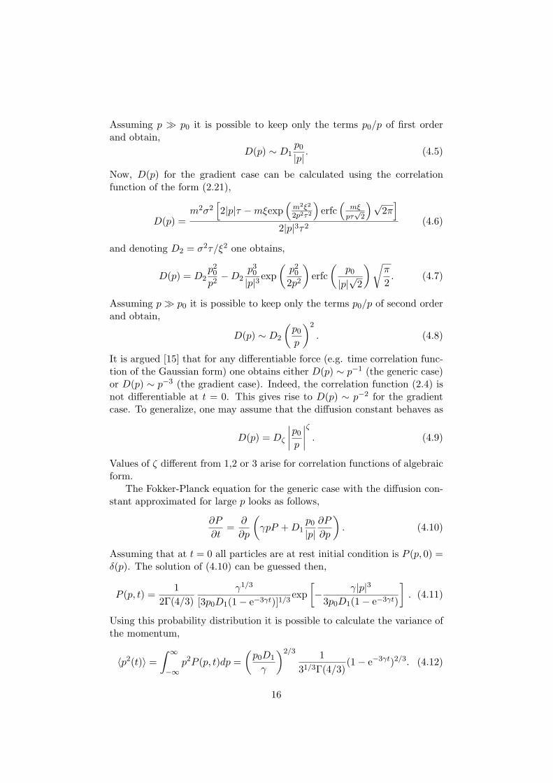
Numerical evaluation of (5.24) as a function of ζ is shown in Fig. 5.7. It canbe seen that for small values ζ it approaches 0 whereas for ζ = 0 it shouldreproduce the result for the standard Ornstein-Uhlenbeck process, that is2/3. Reliable results for small values of ζ are not recovered, however other

30

0.0 0.5 1.0 1.5 2.0 2.5 3.0 3.50.3

0.4

0.5

0.6

0.7

I (

)

Figure 5.7: Numerical evaluation of the integral (5.24) as a function of ζ(solid line)

values are quite precise. Using the numerical values for I(ζ) one can rewrite(5.23) for the generic case,

〈x2(t)〉 = 0.5705× (p0D1)2/3m−2t8/3 (5.25)

and for the gradient case,

〈x2(t)〉 = 0.4580× (p20D2)1/2m−2t5/2. (5.26)

These results agree with the numerical simulations quite well (Figs. 5.2-5.5).

31

Chapter 6

Motion in two spatialdimensions

This chapter gives a brief discussion for the case of motion in two spatialdimensions. In this case the equation of motion replacing (1.2) is,

dp

dt= −γp + f(x, t), (6.1)

where p = (px, py)T , x = (x, y)T and f = (fx, fy)T are two-dimensionalvectors (superscript T denotes transposition). One can consider severalpossibilities of how the random force field f can be generated (see e.g. [11]).One possibility is a potential field,

f(x, t) =(

∂xφ(x, t)∂yφ(x, t)

)(6.2)

where φ is a generic random field described in chapter 2. Another possibilityis a solenoidal (or rotational) field that looks as follows,

f(x, t) =(

∂yφ(x, t)−∂xφ(x, t)

)(6.3)

To generalize, one can also consider a combination of a potential and asolenoidal field,

f(x, t) = α

(∂xψ(x, t)∂yψ(x, t)

)+ β

(∂yφ(x, t)

−∂xφ(x, t)

), (6.4)

where ψ and φ are independent generic random field having identical statis-tical properties, and α and β are real numbers.

The Fokker-Planck equation for the two-dimensional case is derived anal-ogously to the one-dimensional case. One obtains,

∂P (p, t)∂t

= ∇Tp (γpP + D(p)∇pP ) , (6.5)

32

10-1 100 101 102101

102

103

10-1 100 101 10210-3

10-1

101

103

105

107

<p x

2 (t) +

py 2 (t)

>

t

<x

2 (t) +

y 2 (t)

>

t

Figure 6.1: Numerical simulations (circles) for two-dimensional generalizedOrnstein-Uhlenbeck process for the case of potential force field. Red linesshow slope 1/2 for the momentum and 5/2 for the displacement

where∇p denotes a gradient with respect to p and D(p) is a diffusion matrix.It is defined as follows [19],

D(p) =(

D11 D12

D21 D22

), (6.6)

with

D11 =12

∫ ∞

−∞cxx(pt/m, t) dt, (6.7)

D12 = D21 =12

∫ ∞

−∞cxy(pt/m, t) dt,

D22 =12

∫ ∞

−∞cyy(pt/m, t) dt,

where cxx, cxy and cyy are correlation functions of components of f, that is

cxx(x, y, t) = 〈fx(x1, y1, t1)fx(x1 + x, y1 + y, t1 + t)〉, (6.8)cxy(x, y, t) = 〈fx(x1, y1, t1)fy(x1 + x, y1 + y, t1 + t)〉,cyy(x, y, t) = 〈fy(x1, y1, t1)fy(x1 + x, y1 + y, t1 + t)〉.

It is convenient to transform p to polar coordinates as follows,

px = p cos θ, (6.9)py = p sin θ.

As before, the case of large forcing and small damping is considered, that

33

10-1 100 101 102

102

103

104

10-1 100 101 10210-3

10-1

101

103

105

107

109

<p x

2 (t) +

py 2 (t)

>

t

<x

2 (t) +

y 2 (t)

>

t

Figure 6.2: Numerical simulations (circles) for two-dimensional generalizedOrnstein-Uhlenbeck process for the case of solenoidal force field. Red linesshow slope 2/3 for the momentum and 8/3 for the displacement

is |p| À p0. In this limit the diffusion matrix in polar coordinates is

D(p) =D2p0

p

(sin2 θ − cos θ sin θ− cos θ sin θ cos2 θ

)(6.10)

for the potential force field, and

D(p) =D2p0

p

(cos2 θ cos θ sin θcos θ sin θ sin2 θ

)(6.11)

for the solenoidal one. Here, D2 is the same as it was defined in chapter 4.It is, however, not obvious that an approximation of the diffusion matrix

should be carried out before it is used in the Fokker-Planck equation. In fact,the diffusion matrices in the case of the Gaussian time correlation functionare equal to those obtained above. This would imply the same result forboth types of correlation function. Numerical results performed for thecorrelation function of the form (2.4) are consistent with short-time scalingbehaviours obtained in [13] (〈|p|2〉 ∼ t1/2) for the Gaussian time correlationfunction and potential force field (Fig. 6.1). Yet, it is believed that theresults obtained in [13] for multi-dimensional cases are not correct and oneshould refer to [14] where the result is 〈|p|2〉 ∼ t2/5. For the solenoidal forcefield numerical simulations give 〈|p|2〉 ∼ t2/3 (Fig. 6.2)

34

Chapter 7

Conclusions and future work

The most important property of the generalized Ornstein-Uhlenbeck pro-cess may be the fact that the spectrum of the corresponding Fokker-Planckoperator consists of two rows of eigenvalues λ+

n and λ−n that are evenlyspaced in each row, and the rows are staggered with respect to each other.Such a spectrum was called as staggered ladder spectrum in [15]. Usingthe spectral decomposition of the Fokker-Planck operator, correlations andfluctuations of observables in generalized Ornstein-Uhlenbeck process couldbe calculated analytically. It is found that the momentum variance exhibitsanomalous diffusion at short times and grows until particles accelerate toa certain level, but then saturates in equilibrium. The mean square valueof the displacement also exhibits anomalous spatial diffusion at short times,however, at long times an expected result, that is, ordinary diffusion, is con-firmed. The spectral decomposition approach makes it possible to determinein a very clear way many other quantities that are related to momentum of aparticle. Among such quantities, the correlation function of the momentumin equilibrium has been calculated; it decays exponentially for long timebut faster than exp(−γt) as in the standard Ornstein-Uhlenbeck process.The Fokker-Planck equation also gives the probability distribution of themomentum as a function of time, which turns out to be non-Maxwellian inequilibrium for the generalized Ornstein-Uhlenbeck process, unlike Gaussiandistribution for the standard one. The theory has been successfully verifiedby numerical experiments.

In chapter 6, it has been shown that numerical results for the case ofmotion in two spatial dimensions are not consistent with the analytical onesobtained in [14]. The reason for this inconsistence could be the differencein time correlation functions, however the diffusion matrices approximatedfor the case of large p turn out to be the same for both types of correlationfunction. Thus a careful investigation of motion in two spatial dimensionsis the next question to address.

35

Bibliography

[1] J. Schumacher and B. Eckhardt, Phys. Rev. E, 66, 017303 (2002)

[2] E. Balkovsky, G. Falkovich and A. Fouxon, Phys. Rev. Lett., 86, 13(2001)

[3] T. Elperin and N. Kleeorin, Phys. Rev. Lett., 77, 27, 1996

[4] G. Falkovich, K. Gawedzki and M. Vergassola, Rev. Mod. Phys., 73, 913(2001)

[5] K. Duncan, B. Mehlig, S. Ostlund, and M. Wilkinson, Phys. Rev. Lett72, 051104(R), (2005)

[6] A. Einstein, Ann. d. Physik 17, 549 (1905)

[7] M. v. Smoluchowski, Phys. Zeits. 17, 557 (1916)

[8] G. E. Ornstein and L. S. Uhlenbeck, Phys. Rev., 36, 823 (1930).

[9] J. Deutsch, J. Phys. A 18, 1449 (1985)

[10] M. Wilkinson and B. Mehlig, Phys. Rev. E 68, 040101(R), (2003)

[11] B. Mehlig and M. Wilkinson, Phys. Rev. Lett. 92, 250602 (2004)

[12] B. Mehlig, M. Wilkinson, K. Duncan, T. Webber, M. Ljunggren, Phys.Rev. E 95, 240602, (2005)

[13] L. Golubovic, S. Feng, and F.-A. Zeng, Phys. Rev. Lett. 67, 2115 (1991)

[14] M. N. Rosenbluth, Phys. Rev. Lett., 69, 1831, (1992).

[15] E. Arvedson, B. Mehlig, M. Wilkinson, and K. Nakamura, Phys. Rev.Lett. 96 030601 (2006).

[16] H. Sigurgeirsson and A. Stuart, Phys. Fluids 14, 12 (2002)

[17] H. Sigurgeirsson, A. Stuart and Wing-Lok Wan, J. Comp. Phys. 172,766-807 (2001)

36

[18] P. A. Sturrock, Phys. Rev. 141, 186 (1966)

[19] N. G. van Kampen, Stochastic processes in physics and chemistry, 2nded., North-Holland, Amsterdam 1981

[20] I.S. Gradshteyn, I.M. Ryzhik, Table of integrals, series, and products,4th ed., Academic Press, London 1980

[21] V. Bezuglyy, B. Mehlig, M. Wilkinson, K. Nakamura, and E. Arvedson,preprint (2006)

[22] V. Bezuglyy, B. Mehlig, M. Wilkinson, K. Nakamura, A multiplicity ofregimes of diffusion, unpublished (2006)

[23] P. A. M. Dirac, The principles of Quantum Mechanics, Oxford Univer-sity Press, Oxford, (1930).

37