max-margin dictionary learning for multiclass image...

Max-Margin Dictionary Learning for MulticlassImage Categorization

Xiao-Chen Lian1, Zhiwei Li3, Bao-Liang Lu1,2, and Lei Zhang3

1Dept. of Computer Science and Engineering, Shanghai Jiao Tong University, China2MOE-MS Key Lab for BCMI, Shanghai Jiao Tong University, China

3Microsoft Research Asia

Abstract. Visual dictionary learning and base (binary) classifier train-ing are two basic problems for the recently most popular image cate-gorization framework, which is based on the bag-of-visual-terms (BOV)models and multiclass SVM classifiers. In this paper, we study new algo-rithms to improve performance of this framework from these two aspects.Typically SVM classifiers are trained with dictionaries fixed, and as a re-sult the traditional loss function can only be minimized with respectto hyperplane parameters (w and b). We propose a novel loss functionfor a binary classifier, which links the hinge-loss term with dictionarylearning. By doing so, we can further optimize the loss function withrespect to the dictionary parameters. Thus, this framework is able tofurther increase margins of binary classifiers, and consequently decreasethe error bound of the aggregated classifier. On two benchmark dataset,Graz [1] and the fifteen scene category dataset [2], our experiment resultssignificantly outperformed state-of-the-art works.

1 Introduction

Visual recognition is one of the fundamental challenges in computer vision, whichtargets at automatically assigning class labels to images based on their visualfeatures. In recent years, many methods have been proposed [2–5], in which theframework that combines bag of visual words (BOV) model with SVM-basedmulticlass classifiers [3, 4] has achieved state-of-the-art performance in variousbenchmark tasks [2, 6, 7]. To further improve the performance of this framework,we study two basic problems of it in this paper.

First, how to learn a better BOV model? A core issue of this frameworkis generating a dictionary that will be effective for classifier training. Most ofexisting approaches adopt unsupervised clustering manners, whose goals are tokeep sufficient information for representing the original features by minimizing areconstruction error or expected distortion (e.g. K-means [8], manifold learning[9] and sparse coding [4]). Due to the ignorance to supervisory information,the histogram representations of images over the learned dictionary may not beoptimal for a classification task. Therefore, a highly probably better choice isto incorporate discriminative information (i.e. class labels) into the dictionaryconstruction process.

2 X.C. Lian, Z. Li, B.L. Lu and L. Zhang

Second, how to train a better SVM classifier? SVM-based multiclass clas-sifiers are usually constructed by aggregating results of a collection of binaryclassifiers. The most popular strategies are one-vs.-one where all pairs of classesare compared, and one-vs.-all where each class is compared against all others.The performance of the binary classifiers directly affects the performance ofthe aggregated classifier. Thus, a straightforward idea to improve the multiclassclassifiers is improving the individual binary classifier.

Existing approaches typically deal with the above two problems separately:dictionaries are first generated and classifiers are then learned based on them.In this paper, we propose a novel framework for image classification which uni-fies the dictionary learning process with classifier training. The framework re-duces the multiclass problem to a collection of one-vs-one binary problems. Foreach binary problem, classifier learning and dictionary generation are conductediteratively by minimizing a unified objective function which adopts the maxi-mum margin criteria. We name this approach Max-Margin Dictionary Learn-ing (MMDL). We evaluate MMDL using two widely used classifier aggregationstrategies: majority voting and Decision Directed Acyclic Graph (DDAG) [10].Experimental results show that by embedding the dictionary learning into classi-fier training, the performance of the aggregated multiclass classifier is improved.Our results outperformed state-of-the-art results on Graz [1] and the fifteen scenecategory dataset [2].

2 Related Work

Supervised dictionary learning has attracted much attention in recent years.Existing approaches can be roughly categorized into three categories.

First, constructing multiple dictionaries, e.g. [11] wraps dictionary construc-tion inside a boosting procedure and learns multiple dictionaries with comple-mentary discriminative power, and[12] learns a category-specific dictionary foreach category.

Second, learning a dictionary by manipulating an initial dictionary, e.g. merg-ing visual words. The merging process could be guided by mutual information be-tween visual words and classes [13], or trade-off between intra-class compactnessand inter-class discrimination power [14]. The performance of such approaches ishighly affected by the initial dictionary since only merging operation is consid-ered in them. To ease this problem a large dictionary is required at the beginningto preserve as much discriminative abilities as possible, which is not guaranteedthough.

Third, learning a dictionary via pursuing a descriptor-level discriminativeability, e.g. empirical information loss minimization method [15], randomizeddecision forests [16, 17], and sparse coding-based approaches [18–20]. Most ofthese approaches are first motivated from coding of signals, where a sample (orsay signal) is only analogous to a local descriptor in an image rather than awhole image which is composed of a collection of local descriptors. Actually, this

Max-Margin Dictionary Learning for Multiclass Image Categorization 3

requirement is over strong since local descriptors of different objects are oftenoverlapped (i.e. a white patch may appear both in the sky and on a wall).

Moreover, depending on whether dictionary learning and classifier trainingare unified in a single process or not, the above approaches can be further catego-rized to two categories. Most of them take two separate processes, e.g. [11, 16, 17,12–15], in which a dictionary is first learned and then a classifier is trained overit. Therefore, the objectives of the two processes are likely to be inconsistent.The other category of approaches takes a similar strategy as ours, that is, theycombine the two processes by designing a hybrid generative and discriminativeenergy function. The discrimination criteria used include softmax discriminativecost functions [18, 19] and Fisher’s discrimination criterion [20]. However, ex-isting approaches put the discrimination criteria on individual local descriptorsrather than image-level representations, i.e. histogram representations of images.

After this paper was submitted, two additional related works were published,which also consider learning dictionary with image-level discriminative criteria.Yang et al. [27] used sparse coding for dictionary learning and put a classificationloss in the model. Boureau et al. used regularized logistic cost.

3 Max-Margin Dictionary Learning

In this section, we first introduce the motivation of incorporating max-margin cri-teria into dictionary learning process. Then the Max-Margin Dictionary Learning(MMDL) algorithm is described and the analysis on how max-margin criterionaffects the dictionary construction is given. Finally, we describe the pipeline ofthe whole classification framework.

3.1 Problem Formulation

Suppose we are given a corpus of training images D = {(Id, cd)}Dd=1, where Id =

{xd1, x

d2 . . . , xd

Nd} is the set of local descriptors (i.e. SIFT [21]) extracted from

image d, and cd ∈ {+1,−1} is the class label associated with Id. A dictionarylearning method will construct a dictionary which consists of K visual words V ={v1, v2, . . . , vK}. A descriptor xd

i from image d is quantized to a K-dimensionvector φd

i where

φdi [k] =

1, k = argminw

‖ xdi − vw ‖2

0, otherwise(1)

for hard assignment and

φdi [k] =

exp(−γ ‖ xdi − vk ‖22)∑K

k′=1 exp(−γ ‖ xdi − vk′ ‖22)

, k = 1, . . . , K (2)

for soft assignment [22]. Then image d is represented by the histogram

Φd =1

Nd

Nd∑

i=1

φdi , (3)


(a) (b) (c)

Fig. 1. (a) The 2-D synthetic data. Colors of points indicate their categories. (b) K-means results and Voronoi boundary of the words. Red and yellow points are groupedonto the same word and as a result cannot be distinguished. (c) A correct partitionwhere categories information are completely preserved at the price of distortion. Thisfigure should best be viewed in color

and the set of couples {(Φd, cd)} are used to train the classifiers.Traditionally, the dictionary V is learned by minimizing the reconstruction

error or overall distortion. For example, K-means clustering algorithm solves thefollowing problem

minV

D∑

d=1

Nd∑

i=1

mink=1...K

‖ xdi − vk ‖22 (4)

However, as the learning process does not utilize the category information, theresulted histograms may not be optimal for classification. We illustrate the prob-lem on a toy data shown in Figure 1(a). K-means groups the red and yellowclusters into one word (Figure 1(b)) and separates the two green clusters to twowords because it only considers to minimizing the overall distortion. As a result,red and yellow clusters cannot be distinguished through their histogram repre-sentations. A correct partition is shown in Figure 1(c); although the dictionaryhas a bigger distortion, it is more discriminative than the dictionary obtainedby K-means.

3.2 MMDL

Our solution to the above problem is to combine classifier training and dictionarylearning together. Motivated by the loss function in SVM, we design the followingobjective function

L(V, W ) =12‖ W ‖22 +C

∑

d

max(0, 1− cd〈W,Φd〉) (5)

where Φd is computed through Eq. (2) and (3), W = (w1, . . . , wK)> is a hyper-plane classifier and C is the trade-off factor. It is noted that:

1) We omit the offset (i.e. b in a standard SVM classifier) since the L1-normof Φd is always one.


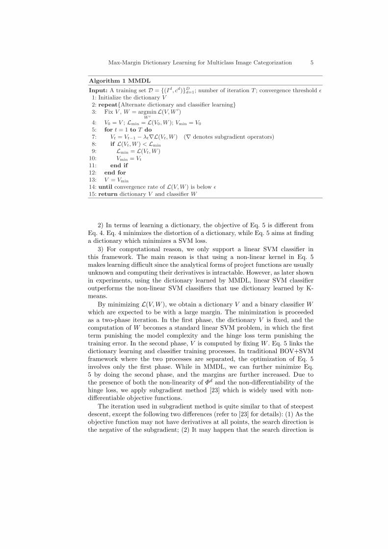
Algorithm 1 MMDL

Input: A training set D = {(Id, cd)}Dd=1; number of iteration T ; convergence threshold ε

1: Initialize the dictionary V2: repeat{Alternate dictionary and classifier learning}3: Fix V , W = argmin

W ′L(V, W ′)

4: V0 = V ; Lmin = L(V0, W ); Vmin = V0

5: for t = 1 to T do7: Vt = Vt−1 − λt∇L(Vt, W ) (∇ denotes subgradient operators)8: if L(Vt, W ) < Lmin

9: Lmin = L(Vt, W )10: Vmin = Vt

11: end if12: end for13: V = Vmin

14: until convergence rate of L(V, W ) is below ε15: return dictionary V and classifier W

2) In terms of learning a dictionary, the objective of Eq. 5 is different fromEq. 4. Eq. 4 minimizes the distortion of a dictionary, while Eq. 5 aims at findinga dictionary which minimizes a SVM loss.

3) For computational reason, we only support a linear SVM classifier inthis framework. The main reason is that using a non-linear kernel in Eq. 5makes learning difficult since the analytical forms of project functions are usuallyunknown and computing their derivatives is intractable. However, as later shownin experiments, using the dictionary learned by MMDL, linear SVM classifieroutperforms the non-linear SVM classifiers that use dictionary learned by K-means.

By minimizing L(V, W ), we obtain a dictionary V and a binary classifier Wwhich are expected to be with a large margin. The minimization is proceededas a two-phase iteration. In the first phase, the dictionary V is fixed, and thecomputation of W becomes a standard linear SVM problem, in which the firstterm punishing the model complexity and the hinge loss term punishing thetraining error. In the second phase, V is computed by fixing W . Eq. 5 links thedictionary learning and classifier training processes. In traditional BOV+SVMframework where the two processes are separated, the optimization of Eq. 5involves only the first phase. While in MMDL, we can further minimize Eq.5 by doing the second phase, and the margins are further increased. Due tothe presence of both the non-linearity of Φd and the non-differentiability of thehinge loss, we apply subgradient method [23] which is widely used with non-differentiable objective functions.

The iteration used in subgradient method is quite similar to that of steepestdescent, except the following two differences (refer to [23] for details): (1) As theobjective function may not have derivatives at all points, the search direction isthe negative of the subgradient; (2) It may happen that the search direction is


not a descent direction, therefore a list recording the lowest objective functionvalue found so far is maintained.

Algorithm 1 depicts the complete MMDL algorithm. In line 3, W is computedby a standard SVM solver. In line 7, the dictionary V is updated according to thesubgradient and the step size λt. The subgradient of a convex function f at pointx0 is a nonempty closed interval [f−(x0), f+(x0)] where f−(x0) and f+(x0) arethe left- and right-sided derivatives respectively. The interval reduces to a pointwhen f is differentiable at x0. In this case, f−(x0) = f+(x0) = ∂f(x0).

Denote 〈W>, Φd〉 by hd(V ), then the hinge loss term for image d is Ld =max(0, 1− cdhd(V )). When cdhd(V ) < 1, Ld = 1− cdhd(V ) is differentiable. Itssubgradient at vk(k = 1 . . . ,K) equals to its derivative

∂Ld

∂vk=

∂

∂vk(−cdwk

Nd

Nd∑

i=1

φdi [k])

= −cdwk

Nd

Nd∑

i=1

2γ(xdi − vk) exp(−γ ‖ xd

i − vk ‖22)(∑Kk′=1 exp(−γ ‖ xd

i − vk′ ‖22))

+cdwk

Nd

Nd∑

i=1

2γ(xdi − vk) exp(−γ ‖ xd

i − vk ‖22)2(∑Kk′=1 exp(−γ ‖ xd

i − vk′ ‖22))2

= −2cdwk

Nd

Nd∑

i=1

γ(xdi − vk)

(φd

i [k]− (φdi [k])2

).

(6)

When cdhd(V ) ≥ 1, the subgradient ∇Ld = 0 for all vk(k = 1 . . . ,K), whichmeans we pick the right-sided derivative of the hinge loss term. The visual wordvk is then updated by

vt+1k = vt

k − λt

∑

d∈X

∂Ld

∂vtk

(7)

where X = {d | cdhd(V ) < 1} is the set of indices of the images that lie inthe margin or are misclassified by W . We name these images as effective imagesbecause only these images are involved in the dictionary update equation.

Analysis We examine the update rules to see how the effective images takeeffect in the dictionary learning process. For better understanding, we reformatEq. (7) as:

v′k = vk +∑

d∈X

2γλ

Nd

Nd∑

i=1

sdi [k] · tdi [k] · pd

i [k], (8)

wheresd

i [k] = sign(cdwk)

pdi [k] =

xdi − vk

‖ xdi − vk ‖22

tdi [k] = wk

(φd

i [k]− (φdi [k])2

) ‖ xdi − vk ‖22 .

(9)


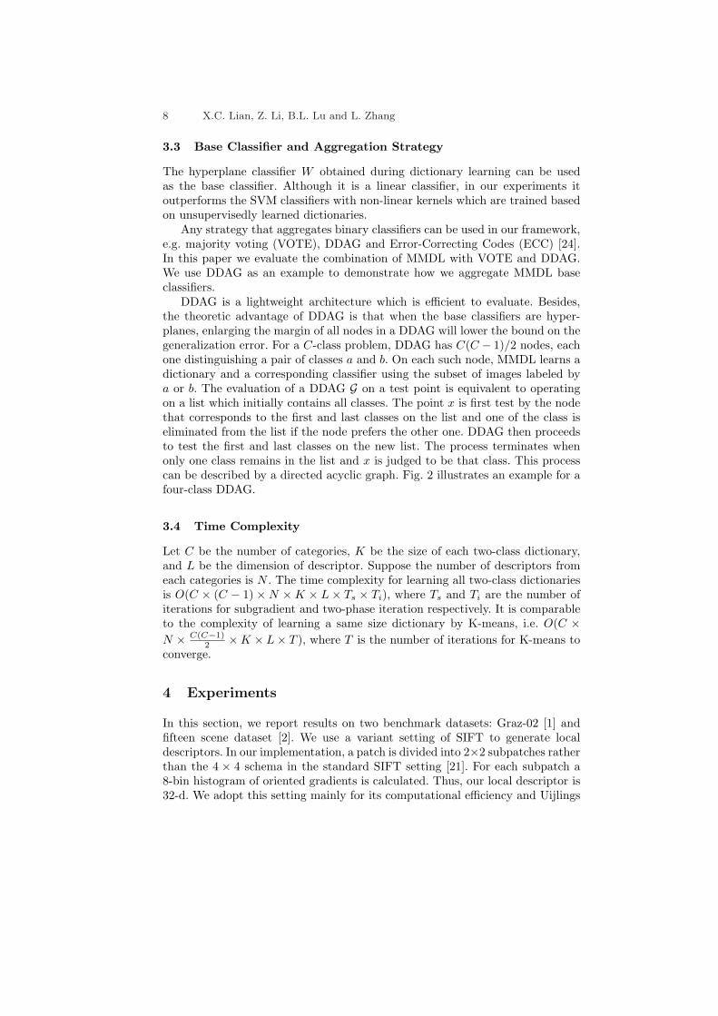
Fig. 2. A four-class DDAG. The list under each node contains the class labels that willremain when the evaluation reaches the node

Intuitively, the update of vk is the net force of all local descriptors in effectiveimages. Each descriptor xd

i pushes or pulls vk along a direction. The directionof the force is determined by sd

i [k] and pdi [k]. If sd

i [k] > 0, it means that thek-th word is positive to correctly predicting the label of image d (i.e. the imagefavors larger φd

i [k]); otherwise, it means that we expect that the image d shouldhave smaller φd

i [k]. As a result, when sdi [k] > 0, vk will be pulled to be near to

descriptor xdi , and when sd

i [k] < 0, it will be pushed to be far away from xdi .

Therefore moving vk according to Eq. (8) will decreases the hinge loss L(V, W ).The strength of xd

i ’s force on vk is determined by tdi [k], which is proportionalto wk, a quadratic term φd

i [k] − (φdi [k])2 and ‖ xd

i − vk ‖22 (Euclidean distancebetween xd

i and vk). In the following, we give an intuitive explanation abouttdi [k].

From the feature selection’s point of view, hyperplane W plays a role asvisual word selector. If the absolute value of wk is very small, it means the wordis not important for the classifier, and thus the update to the corresponding vk

could be minor.

Before analyzing the latter two terms, we first note that φdi [k] and ed

i [k] =‖xd

i −vk ‖22 are both related to the distance between descriptor xdi and visual word

vk. The former one measures the relative distance from vk to xdi [k] compared with

other visual words, while the latter is the absolute distance. We first consider thecase when the force xd

i exerts on vk is pull. When φdi [k] is very large, moving vk

for a distance may not increase the distortion too much. Therefore the quadraticterm φd

i [k]− (φdi [k])2 will be small, indicating that xd

i does not hold vk stronglyand allows other descriptors to move it. If φd

i [k] is quite small, vk is relativefar from xd

i , and the quadratic term will also be small which means the forceshould be small as moving vk close to xd

i may cause large distortion. If edi is

large but other visual words are much far away from xdi , moving vk close is

acceptable. Otherwise xdi may not pull vk over as the distortion may increase.

Similar discussion can be made when the force is push.


3.3 Base Classifier and Aggregation Strategy

The hyperplane classifier W obtained during dictionary learning can be usedas the base classifier. Although it is a linear classifier, in our experiments itoutperforms the SVM classifiers with non-linear kernels which are trained basedon unsupervisedly learned dictionaries.

Any strategy that aggregates binary classifiers can be used in our framework,e.g. majority voting (VOTE), DDAG and Error-Correcting Codes (ECC) [24].In this paper we evaluate the combination of MMDL with VOTE and DDAG.We use DDAG as an example to demonstrate how we aggregate MMDL baseclassifiers.

DDAG is a lightweight architecture which is efficient to evaluate. Besides,the theoretic advantage of DDAG is that when the base classifiers are hyper-planes, enlarging the margin of all nodes in a DDAG will lower the bound on thegeneralization error. For a C-class problem, DDAG has C(C − 1)/2 nodes, eachone distinguishing a pair of classes a and b. On each such node, MMDL learns adictionary and a corresponding classifier using the subset of images labeled bya or b. The evaluation of a DDAG G on a test point is equivalent to operatingon a list which initially contains all classes. The point x is first test by the nodethat corresponds to the first and last classes on the list and one of the class iseliminated from the list if the node prefers the other one. DDAG then proceedsto test the first and last classes on the new list. The process terminates whenonly one class remains in the list and x is judged to be that class. This processcan be described by a directed acyclic graph. Fig. 2 illustrates an example for afour-class DDAG.

3.4 Time Complexity

Let C be the number of categories, K be the size of each two-class dictionary,and L be the dimension of descriptor. Suppose the number of descriptors fromeach categories is N . The time complexity for learning all two-class dictionariesis O(C × (C − 1) ×N ×K × L × Ts × Ti), where Ts and Ti are the number ofiterations for subgradient and two-phase iteration respectively. It is comparableto the complexity of learning a same size dictionary by K-means, i.e. O(C ×N × C(C−1)

2 ×K × L× T ), where T is the number of iterations for K-means toconverge.

4 Experiments

In this section, we report results on two benchmark datasets: Graz-02 [1] andfifteen scene dataset [2]. We use a variant setting of SIFT to generate localdescriptors. In our implementation, a patch is divided into 2×2 subpatches ratherthan the 4 × 4 schema in the standard SIFT setting [21]. For each subpatch a8-bin histogram of oriented gradients is calculated. Thus, our local descriptor is32-d. We adopt this setting mainly for its computational efficiency and Uijlings


Table 1. A comparison of the pixel precision-recall equal error rates on Graz-02dataset. Dictionary size is 200

cars people bicycles

AIB200-KNN [13] 50.90 49.70 63.80

AIB200-SVM [13] 40.10 50.70 59.90

MMDL+HP 54.27 55.81 63.55

et al. [25] reported that 2×2 SIFT performed marginally better but never worsethan the 4× 4 SIFT.

In all experiments, we perform processing in gray scale, even when color im-ages are available. We initialize the dictionary V by randomly selecting descrip-tors from training data and set the parameters of MMDL as C = 32, γ = 1×10−3

and λt = 1×10−1 for all t = 1 . . . , T . The number of iterations T for subgradientmethod is set to be 40, and MMDL converges after about 30 iterations underthe convergence threshold ε = 1× 10−4.

4.1 Object Localization

We first use Graz-02 dataset [1] to evaluate the performance of MMDL for ob-ject localization. Graz-02 contains three classes (bicycles, cars and people) withextreme variability in pose, scale and lighting. The task is to label image pixel aseither belonging to one of the three classes or background. The baseline approachis another supervised dictionary learning method proposed in [13]. The measureof performance is pixel precision-recall error rate. We follow the same setup asin [13]: for each object, a dictionary that distinguishes foreground objects frombackground is constructed; when testing, a histogram of frequencies of visualwords within the 80 × 80-pixel window centered at each pixel is computed. ASVM classifier is applied to classify the histogram and a confidence that the pixelbelongs to foreground object is returned. Precision and recall are computed ac-cording to ground-truth segmentation provided by the dataset. The results whenthe sizes of dictionaries are 200 are reported in Table 1. MMDL+HP means thatwe directly used the learned hyperplane classifiers obtained during the dictio-nary learning. The performance of our approach is significantly better than thebaseline approach on the first two classes, and is comparable with [13] on thelast class.

4.2 Scene Category Classification

The second dataset we use is the fifteen scene dataset (scene15), which consistsof fifteen kinds of scene images, e.g. highway, kitchen and street. As in [2, 15],SIFT descriptors of 16× 16 patches sampled over a grid with spacing of 8 pixelsare computed. 100 images per class are randomly selected for training and therest for testing. We train 105 binary classifiers, one for each pair of classes,


20 40 60 80 1000

50

100

150

200

250

300

hing

e lo

ss

KM+LNMMDL+LNMMDL+HP

Fig. 3. Comparison of hinge losses on all binary problems obtained by MMDL andK-means on scene15. The hinge losses are computed on test data

Table 2. Comparison of hinge losses for the top four most confused classes of scene15:bedroom, kitchen, living room and industrial

KM+LN MMDL+LN MMDL+HP

bedroom vs. kitchen 137.25± 8.23 115.86± 3.56 108.59± 6.35bedroom vs. living room 239.97± 9.55 206.62± 13.08 189.93± 32.36bedroom vs. industrial 168.38± 2.87 124.71± 0.49 125.25± 5.89kitchen vs. living room 193.47± 9.70 173.29± 14.23 166.30± 12.70kitchen vs. industrial 133.34± 16.91 95.78± 7.56 88.24± 8.24living room vs. industrial 222.74± 24.41 147.55± 33.33 155.82± 16.33

with all possible combinations of dictionary learning algorithms and classifiersettings. The dictionary learning algorithms are K-means (KM) and MMDL.The quantization of KM uses the soft assignment in Eq. 2 with the same γas MMDL. Each binary problem use a dictionary with 50 visual words. Theclassifiers are SVM with linear kernel (LN) and histogram intersection kernel(HI), and the hyperplane-based classifier learned by MMDL (HP). For example,a name “KM+HI+DDAG” means that we adopt K-means to learn a dictionary,histogram intersection kernel to train SVM classifiers, and the DDAG approachto aggregate base classifiers. The experiments are repeated five times and thefinal result is reported as the mean and standard deviation of the results fromthe individual runs.

To show the superiority of MMDL over K-means, in Fig. 3 we plot the hingelosses of linear classifiers on all binary problems obtained by the K-means andMMDL. The x-coordinate is the indices of binary classifiers which are sorted inan order that their hinge loss produced by the corresponding KM+LIN methodon test set are ascending. We also list the hinge losses of the top four mostconfused classes (bedroom, kitchen, living room and industrial) in Table 2. In


20 40 60 80 1000.65

0.7

0.75

0.8

0.85

0.9

0.95

1

prec

isio

n

KM+LNMMDL+LNMMDL+HP

Fig. 4. Comparison of precisions on all binary problems obtained by MMDL and K-means on scene15

Table 3. Comparison of precisions (percentage) for the top four most confused classesof scene15: bedroom, kitchen, living room and industrial

KM+LN MMDL+LN MMDL+HP

bedroom vs. kitchen 77.46± 2.38 80.04± 0.97 82.69± 1.11bedroom vs. living room 66.70± 0.42 70.06± 3.26 72.37± 0.77bedroom vs. industrial 81.96± 1.84 86.99± 1.43 87.83± 1.51kitchen vs. living room 72.03± 1.43 75.86± 3.37 78.53± 2.26kitchen vs. industrial 86.80± 1.92 86.96± 0.39 89.60± 1.41living room vs. industrial 78.66± 2.73 87.55± 3.37 85.56± 0.94

the similar way, we compare their precisions on all binary problems in Fig. 4 andTable 3. We can see that:

1) In terms of both the hinge loss and precision, MMDL based approach issignificantly better than K-means based approaches.

2) For the four categories, which KM+LIN does not distinguish well (i.e.classification between the four classes), the improvements obtained by MMDLare significant. For all categories, MMDL outperforms K-means.

Table 4 shows the performance for each category with different dictionaryand classifier settings. Our basic approaches, i.e. MMDL+HP+DDAG/VOTE,significantly outperform the baseline approaches (KM+HI+DDAG/VOTE), andwith histogram intersection kernel, their performance is even better. With a 200word universal dictionary, which is obtained by running K-means over SIFT de-scriptors of randomly sampled 400 images, the linear SVM achieved an averageprecision at 74.3%1 which is also lower than our approaches. We also learneda 5250-word universal dictionary by K-means, whose size is equal to the totalnumber of visual words used in MMDL approaches. Its result with histogramintersection kernel is 75.3%. An interesting observation is that without incor-

1 The result is better than the result, 72.2± 0.6%, reported in [2]


Table 4. Comparison of precisions (percentage) for all classes of scene15

KM+HI MMDL+HP MMDL+HIclass DDAG VOTE DDAG VOTE DDAG VOTE

bedroom 34.5± 0.9 40.8± 1.8 47.1± 7.3 58.0± 5.2 46.0± 5.7 55.7± 5.7suburb 88.2± 3.9 89.4± 2.5 91.7± 1.1 92.9± 2.6 92.9± 1.9 93.9± 1.8kitchen 52.1± 1.4 57.0± 3.4 71.2± 0.5 69.4± 3.4 68.8± 6.7 69.1± 6.3living room 49.7± 3.8 46.9± 4.2 53.3± 1.3 51.0± 5.0 61.9± 2.4 54.1± 3.8coast 81.0± 5.3 82.6± 5.5 82.4± 1.2 84.6± 2.0 86.2± 2.8 90.1± 3.1forest 90.2± 1.3 90.8± 1.6 92.3± 1.5 92.3± 1.5 90.6± 1.8 91.7± 1.2highway 83.8± 3.8 84.4± 2.5 87.1± 1.8 87.1± 2.4 87.1± 2.5 88.1± 3.5inside city 65.2± 3.9 66.8± 3.5 72.1± 3.8 72.8± 3.6 72.6± 1.7 75.8± 1.1mountain 79.2± 1.8 78.5± 2.4 83.8± 1.3 82.1± 1.6 84.4± 1.1 82.5± 1.3open country 68.4± 2.6 68.0± 2.9 71.5± 1.5 73.4± 3.2 80.0± 2.1 78.8± 2.3street 84.0± 2.4 82.6± 2.9 87.3± 2.1 86.5± 1.4 86.1± 1.5 86.3± 2.1tall building 82.9± 0.6 82.0± 0.7 77.9± 1.0 79.0± 5.6 87.5± 1.0 85.3± 0.2office 77.4± 1.5 75.9± 2.0 82.9± 4.8 80.9± 3.0 89.3± 4.0 87.5± 5.8store 64.0± 5.8 63.1± 6.2 68.2± 1.2 70.7± 3.3 74.6± 0.5 73.8± 0.5industrial 42.3± 5.2 42.0± 2.8 42.2± 5.0 48.3± 4.8 55.5± 4.3 58.5± 5.2

average 69.5± 0.2 70.1± 0.1 74.1± 1.2 75.3± 2.1 77.6± 0.3 78.1± 0.7

porating the max margin term into learning process, using a set of two-classdictionaries is worse than using a single dictionary with enough size. Two-classdictionaries are likely to over fit on training images, and their generalizationcapabilities are usually weak. While from table 4, we can see that MMDL canboost the performance, which is attributed to the incorporation of max margincriteria.

On scene15, the state-of-the-art results are obtained by applying spatial pyra-mid matching (SPM) mechanism [2]. We apply it to each binary classifier in ourframework. Although our objective function of dictionary learning does not op-timize for the SPM representation, our approach achieves the best results asshown in Table 5. To the best of our knowledge, it outperforms all results onthis dataset reported in recent years [3, 4, 2, 26]. Actually, due to a characteristicof SPM mechanism (i.e. it is a “linear” transform indeed), it can be integratedin our loss function easily.

5 Conclusion

We have proposed a max-margin dictionary learning algorithm, which can beintegrated in the training process of a linear SVM classifier to further increasethe margin of the learned classifier, and consequently decrease the error bound ofthe aggregated multi-class classifier. Our preliminary experiment results on twobenchmark datasets demonstrate the effectiveness of the proposed approach.

In the future, we are going to study how to directly apply non-linear kernelfunctions, e.g. histogram intersection kernel and χ2 kernel, in the SVM clas-


Table 5. Comparison of average precisions (percentage) on secene15 dataset

L = 2 L = 3

MMDL+SPM+HP+DDAG 78.34± 0.90 82.33± 0.39MMDL+SPM+HP+VOTE 79.15± 0.76 83.21± 0.45MMDL+SPM+HI+DDAG 82.23± 1.01 85.98± 0.68MMDL+SPM+HI+VOTE 82.66± 0.51 86.43± 0.41KM+SPM+HI+DDAG 77.48± 1.08 79.65± 0.59KM+SPM+HI+VOTE 77.89± 0.50 80.17± 0.28HG [26] - 85.2SPM [2] 80.1± 0.5 81.4± 0.5ScSPM [4] - 80.4± 0.9sPACT [3] - 83.3± 0.5

sifier. Recently, using spatial information in image classification have drawnmuch attention. A common problem of these approaches is that the spatial con-straints are predetermined and fixed during dictionary learning. We are design-ing a method that will automatically determine the spatial constraints under theguidance of supervised information.

Acknowledgments

This research was supported in part by the National Natural Science Foundationof China (Grant No. 60773090 and Grant No. 90820018), the National BasicResearch Program of China (Grant No. 2009CB320901), and the National High-Tech Research Program of China (Grant No. 2008AA02Z315).

References

1. Opelt, A., Pinz, A.: Object localization with boosting and weak supervision forgeneric object recognition. Lecture notes in computer science (3540) 862–871

2. Lazebnik, S., Schmid, C., Ponce, J.: Beyond bags of features: Spatial pyramidmatching for recognizing natural scene categories. In: Proc. CVPR. (2006) 2169–2178

3. Wu, J., Rehg, J.: Where am I: Place instance and category recognition using spatialPACT. In: Proc. CVPR. (2008)

4. Yang, J., Yu, K., Gong, Y., Huang, T.: Linear spatial pyramid matching usingsparse coding for image classification. In: Proc. CVPR. (2009)

5. Fei-Fei, L., Perona, P.: A bayesian hierarchical model for learning natural scenecategories. In: Proc. CVPR. (Volume 2.) 524–531

6. Fei-Fei, L., Fergus, R., Perona, P.: Learning generative visual models from fewtraining examples: An incremental bayesian approach tested on 101 object cate-gories. Comput. Vis. Image Underst. 106 (2007) 59–70

7. Everingham, M., Van Gool, L., Williams, C.K.I., Winn, J., Zisserman, A.: ThePASCAL Visual Object Classes Challenge 2009 Results. (http://www.pascal-network.org/challenges/VOC/voc2009/workshop/index.html)


8. Sivic, J., Zisserman, A.: Video Google: A text retrieval approach to object matchingin videos. In: Proc. ICCV. Volume 2. (2003) 1470–1477

9. Jiang, Y.G., Ngo, C.W.: Visual word proximity and linguistics for semantic videoindexing and near-duplicate retrieval. Comput. Vis. Image Underst. 113 (2009)405–414

10. Platt, J., Cristianini, N., Shawe-Taylor, J.: Large margin DAGs for multiclassclassification. Advances in neural information processing systems 12 (2000) 547–553

11. Zhang, W., Surve, A., Fern, X., Dietterich, T.: Learning non-redundant codebooksfor classifying complex objects. In: Proceedings of the 26th Annual InternationalConference on Machine Learning. (2009)

12. Perronnin, F.: Universal and adapted vocabularies for generic visual categorization.IEEE Transactions on Pattern Analysis and Machine Intelligence 30 (2008) 1243–1256

13. Fulkerson, B., Vedaldi, A., Soatto, S.: Localizing objects with smart dictionaries.In: Proc. ECCV, Springer (2008)

14. Winn, J., Criminisi, A., Minka, T.: Object categorization by learned universalvisual dictionary. In: Proc. ICCV. (2005) 1800–1807

15. Lazebnik, S., Raginsky, M.: Supervised learning of quantizer codebooks by in-formation loss minimization. IEEE Trans. Pattern Anal. Mach. Intell. 31 (2009)1294–1309

16. Moosmann, F., Triggs, B., Jurie, F.: Fast discriminative visual codebooks usingrandomized clustering forests. Advances in neural information processing systems19 (2007) 985

17. Shotton, J., Johnson, J., Cipolla, M.: Semantic texton forests for image catego-rization and segmentation. In: Proc. CVPR. (2008)

18. Mairal, J., Bach, F., Ponce, J., Sapiro, G., Zisserman, A.: Supervised dictionarylearning. Advances in Neural Information Processing Systems 21 (2009)

19. Mairal, J., Bach, F., Ponce, J., Sapiro, G., Zisserman, A.: Discriminative learneddictionaries for local image analysis. In: Proc. CVPR. (2008)

20. Huang, K., Aviyente, S.: Sparse representation for signal classification. Advancesin Neural Information Processing Systems 19 (2007) 609

21. Lowe, D.: Object recognition from local scale-invariant features. In: Proc. ICCV.Volume 2. (1999) 1150–1157

22. Philbin, J., Chum, O., Isard, M., Sivic, J., Zisserman, A.: Lost in quantization:Improving particular object retrieval in large scale image databases. In: Proc.CVPR. (2008)

23. Shor, N., Kiwiel, K., Ruszcaynski, A.: Minimization methods for non-differentiablefunctions. Springer-Verlag New York, Inc. New York, NY, USA (1985)

24. Allwein, E., Schapire, R., Singer, Y.: Reducing multiclass to binary: A unifyingapproach for margin classifiers. The Journal of Machine Learning Research 1(2001) 113–141

25. Uijlings, J., Smeulders, A., Scha, R.: What is the Spatial Extent of an Object? In:Proc. CVPR. (2009)

26. Zhou, X., Cui, N., Li, Z. Liang, F., Huang, T.: Hierarchical Gaussianization forImage Classification. In: Proc. ICCV. (2009)

27. Yang, J., K., Y., T., H.: Supervised Translation-Invariant Sparse Coding. In: Proc.CVPR. (2010)

28. Y.L., B., F., B., Y., L., J., P.: Learning Mid-Level Features For Recognition. In:Proc. CVPR. (2010)

max-margin dictionary learning for multiclass image...

Documents