matrix methods - applied linear algebra 3rd ed - bronson,costa.pdf
TRANSCRIPT


MATRIX METHODS

The Student Solutions Manual is now availableonline through separate purchase at
www.elsevierdirect.com/companions/9780123744272

MATRIX METHODS:Applied Linear AlgebraThird Edition
Richard BronsonFairleigh Dickinson UniversityTeaneck, New Jersey
Gabriel B. CostaUnited States Military AcademyWest Point, New York
AMSTERDAM • BOSTON • HEIDELBERG • LONDONNEW YORK • OXFORD • PARIS • SAN DIEGO
SAN FRANCISCO • SINGAPORE • SYDNEY • TOKYO
Academic Press is an imprint of Elsevier

Academic Press is an imprint of Elsevier30 Corporate Drive, Suite 400, Burlington, MA 01803, USA525 B Street, Suite 1900, San Diego, California 92101-4495, USA84 Theobald’s Road, London WC1X 8RR, UK
Copyright © 2009, Elsevier Inc. All rights reserved.
No part of this publication may be reproduced or transmitted in any form or by any means,electronic or mechanical, including photocopy, recording, or any information storage andretrieval system, without permission in writing from the publisher.
Permissions may be sought directly from Elsevier’s Science & Technology Rights Departmentin Oxford, UK: phone: (+44) 1865 843830, fax: (+44) 1865 853333, E-mail: [email protected] may also complete your request online via the Elsevier homepage (http://elsevier.com), byselecting “Support & Contact” then “Copyright and Permission” and then “Obtaining Permissions.”
Library of Congress Cataloging-in-Publication DataAPPLICATION SUBMITTED
British Library Cataloguing-in-Publication DataA catalogue record for this book is available from the British Library.
ISBN: 978-0-12-374427-2
For information on all Academic Press publicationsvisit our Web site at www.elsevierdirect.com
Printed in the United States of America08 09 10 9 8 7 6 5 4 3 2 1

To Evy...again.
R.B.
To my brother priests...especially Father Frank Maione,the parish priest of my youth...and Archbishop Peter
Leo Gerety, who ordained me a priest.
G.B.C.

This page intentionally left blank

Contents
Preface xi
About the Authors xiii
Acknowledgments xv
1 Matrices 1
1.1 Basic Concepts 1Problems 1.1 3
1.2 Operations 6Problems 1.2 8
1.3 Matrix Multiplication 9Problems 1.3 16
1.4 Special Matrices 19Problems 1.4 23
1.5 Submatrices and Partitioning 29Problems 1.5 32
1.6 Vectors 33Problems 1.6 34
1.7 The Geometry of Vectors 37Problems 1.7 41
2 Simultaneous Linear Equations 43
2.1 Linear Systems 43Problems 2.1 45
2.2 Solutions by Substitution 50Problems 2.2 54
2.3 Gaussian Elimination 54Problems 2.3 62
vii

viii Contents
2.4 Pivoting Strategies 65Problems 2.4 70
2.5 Linear Independence 71Problems 2.5 76
2.6 Rank 78Problems 2.6 83
2.7 Theory of Solutions 84Problems 2.7 87
2.8 Final Comments on Chapter 2 88
3 The Inverse 93
3.1 Introduction 93Problems 3.1 98
3.2 Calculating Inverses 101Problems 3.2 106
3.3 Simultaneous Equations 109Problems 3.3 111
3.4 Properties of the Inverse 112Problems 3.4 114
3.5 LU Decomposition 115Problems 3.5 121
3.6 Final Comments on Chapter 3 124
4 An Introduction to Optimization 127
4.1 Graphing Inequalities 127Problems 4.1 130
4.2 Modeling with Inequalities 131Problems 4.2 133
4.3 Solving Problems Using Linear Programming 135Problems 4.3 140
4.4 An Introduction to The Simplex Method 140Problems 4.4 147
4.5 Final Comments on Chapter 4 147
5 Determinants 149
5.1 Introduction 149Problems 5.1 150
5.2 Expansion by Cofactors 152Problems 5.2 155
5.3 Properties of Determinants 157Problems 5.3 161
5.4 Pivotal Condensation 163Problems 5.4 166
Contents ix
5.5 Inversion 167
Problems 5.5 169
5.6 Cramer’s Rule 170
Problems 5.6 173
5.7 Final Comments on Chapter 5 173
6 Eigenvalues and Eigenvectors 177
6.1 Definitions 177
Problems 6.1 179
6.2 Eigenvalues 180
Problems 6.2 183
6.3 Eigenvectors 184
Problems 6.3 188
6.4 Properties of Eigenvalues and Eigenvectors 190
Problems 6.4 193
6.5 Linearly Independent Eigenvectors 194
Problems 6.5 200
6.6 Power Methods 201
Problems 6.6 211
7 Matrix Calculus 213
7.1 Well-Defined Functions 213
Problems 7.1 216
7.2 Cayley–Hamilton Theorem 219
Problems 7.2 221
7.3 Polynomials of Matrices–Distinct Eigenvalues 222
Problems 7.3 226
7.4 Polynomials of Matrices—General Case 228
Problems 7.4 232
7.5 Functions of a Matrix 233
Problems 7.5 236
7.6 The Function eAt 238
Problems 7.6 240
7.7 Complex Eigenvalues 241
Problems 7.7 244
7.8 Properties of eA 245
Problems 7.8 247
7.9 Derivatives of a Matrix 248
Problems 7.9 253
7.10 Final Comments on Chapter 7 254

x Contents
8 Linear Differential Equations 2578.1 Fundamental Form 257
Problems 8.1 2618.2 Reduction of an nth Order Equation 263
Problems 8.2 2698.3 Reduction of a System 269
Problems 8.3 2748.4 Solutions of Systems with Constant Coefficients 275
Problems 8.4 2858.5 Solutions of Systems—General Case 286
Problems 8.5 2948.6 Final Comments on Chapter 8 295
9 Probability and Markov Chains 297
9.1 Probability: An Informal Approach 297Problems 9.1 300
9.2 Some Laws of Probability 301Problems 9.2 304
9.3 Bernoulli Trials and Combinatorics 305Problems 9.3 309
9.4 Modeling with Markov Chains: An Introduction 310Problems 9.4 313
9.5 Final Comments on Chapter 9 314
10 Real Inner Products and Least-Square 31510.1 Introduction 315
Problems 10.1 31710.2 Orthonormal Vectors 320
Problems 10.2 32510.3 Projections and QR-Decompositions 327
Problems 10.3 33710.4 The QR-Algorithm 339
Problems 10.4 34310.5 Least-Squares 344
Problems 10.5 352
Appendix: A Word on Technology 355
Answers and Hints to Selected Problems 357
Index 411

Preface
It is no secret that matrices are used in many fields. They are naturally presentin all branches of mathematics, as well as, in many engineering and science fields.Additionally, this simple but powerful concept is readily applied to many otherdisciplines, such as economics, sociology, political science, nursing and psychology.
The Matrix is a dynamic construct. New applications of matrices are stillevolving, and our third edition of Matrix Methods: Applied Linear Algebra(previouslyAn Introduction) reflects important changes that have transpired sincethe publication of the previous edition.
In this third edition, we added material on optimization and probability theory.Chapter 4 is new and covers an introduction to the simplex method, one of themajor applied advances in the last half of the twentieth century. Chapter 9 isalso new and introduces Markov Chains, a primary use of matrices to probabilityapplications. To ensure that the book remains appropriate in length for a onesemester course, we deleted some of the subject matter that is more advanced;specifically, chapters on the Jordan Canonical Form and on Special Matrices (e.g.,Hermitian and Unitary Matrices). We also included an Appendix dealing withtechnological support, such as computer algebra systems. The reader will also findthat the text contains a considerable “modeling flavor”.
This edition remains a textbook for the student, not the instructor. It remainsa book on methodology rather than theory. And, as in all past editions, proofs aregiven in the main body of the text only if they are easy to follow and revealing.
For most of this book, a firm understanding of basic algebra and a smatteringof trigonometry are the only prerequisites; any references to calculus are few andfar between. Calculus is required for Chapter 7 and Chapter 8; however, thesechapters may be omitted with no loss of continuity, should the instructor wishto do so. The instructor will also find that he/she can “mix and match” chaptersdepending on the particular course requirements and the needs of the students.
xi

xii Preface
In closing, we would like to acknowledge the many people who helped to makethis book a reality. These include the professors, most notably Nicholas J. Rose,who introduced us to the subject matter and instilled in us their love of matrices.They also include the hundreds of students who interacted with us when we passedalong our knowledge to them. Their questions and insights enabled us to betterunderstand the underlying beauty of the field and to express it more succinctly.
Special thanks go to the Most Reverend John J. Myers,Archbishop of Newark,as well as to the Reverend Monsignor James M. Cafone and the Priest Communityat Seton Hall University. Gratitude is also given to the administrative leadersof Seton Hall University, and to Dr. Joan Guetti and to the members of theDepartment of Mathematics and Computer Science. Finally, thanks are given toColonel Michael Phillips and to the members of the Department of MathematicalSciences of the United States Military Academy.
Richard BronsonTeaneck, NJ
Gabriel B. CostaWest Point, NY and South Orange, NJ

About the Authors
Richard Bronson is a Professor of Mathematics in the School of ComputerScience and Engineering at Fairleigh Dickinson University, where he is currentlythe Senior Executive Assistant to the President. Dr. Bronson has been chairmanof his academic department, Acting Dean of his college and Interim Provost. Hehas authored or co-authored eleven books in mathematics and over thirty articles,primarily in mathematical modeling.
Gabriel B. Costa is a Catholic priest. He is a Professor of Mathematical Sciencesand associate chaplain at the United States Military Academy at West Point. He ison an extended Academic Leave from Seton Hall University. His interests includedifferential equations, sabermetrics and mathematics education. This is the thirdbook Father Costa has co-authored with Dr. Bronson.
xiii

This page intentionally left blank

Acknowledgments
Many readers throughout the country have suggested changes and additions tothe first edition, and their contributions are gratefully acknowledged. They includeJohn Brillhart, of the University of Arizona; Richard Thornhill, of the Universityof Texas; Ioannis M. Roussos, of the University of Southern Alabama; RichardScheld and James Jamison, of Memphis State University; Hari Shankar, of OhioUniversity; D.J. Hoshi, of ITT-West;W.C. Pye and Jeffrey Stuart, of the Universityof Southern Mississippi; Kevin Andrews, of Oakland University; Harold Klee,of the University of Central Florida; Edwin Oxford, Patrick O’Dell and HerbertKasube, of Baylor University; and Christopher McCord, Philip Korman, CharlesGroetsch and John King, of the University of Cincinnati.
Special thanks must also go to William Anderson and Gilbert Steiner, of Fair-leigh Dickinson University, who were always available to me for consultationand advice in writing this edition, and to E. Harriet, whose assistance was instru-mental in completing both editions. Finally, I have the opportunity to correct atwenty-year oversight: Mable Dukeshire, previously Head of the Department ofMathematics at FDU, now retired, gave me support and encouragement to writethe first edition. I acknowledge her contribution now, with thanks and friendship.
xv

This page intentionally left blank

11Matrices
1.1 Basic Concepts
Definition 1 A matrix is a rectangular array of elements arranged in horizontalrows and vertical columns. Thus, [
1 3 52 0 −1
], (1)
⎡⎣4 1 1
3 2 10 4 2
⎤⎦, (2)
and ⎡⎣
√2
π
19.5
⎤⎦ (3)
are all examples of a matrix.The matrix given in (1) has two rows and three columns; it is said to have order
(or size) 2 × 3 (read two by three). By convention, the row index is always givenfirst. The matrix in (2) has order 3 × 3, while that in (3) has order 3 × 1. The entriesof a matrix are called elements.
In general, a matrix A (matrices will always be designated by uppercaseboldface letters) of order p × n is given by
A =
⎡⎢⎢⎢⎢⎢⎣
a11 a12 a13 · · · a1n
a21 a22 a23 · · · a2n
a31 a32 a33 · · · a3n...
......
...
ap1 ap2 ap3 · · · apn
⎤⎥⎥⎥⎥⎥⎦, (4)
1

2 Chapter 1 Matrices
which is often abbreviated to [aij]p × n or just [aij]. In this notation, aij representsthe general element of the matrix and appears in the ith row and the jth column.The subscript i, which represents the row, can have any value 1 through p, whilethe subscript j, which represents the column, runs 1 through n. Thus, if i = 2 andj = 3, aij becomes a23 and designates the element in the second row and thirdcolumn. If i = 1 and j = 5, aij becomes a15 and signifies the element in the firstrow, fifth column. Note again that the row index is always given before the columnindex.
Any element having its row index equal to its column index is a diagonalelement. Thus, the diagonal elements of a matrix are the elements in the 1−1position, 2−2 position, 3−3 position, and so on, for as many elements of this typethat exist. Matrix (1) has 1 and 0 as its diagonal elements, while matrix (2) has 4,2, and 2 as its diagonal elements.
If the matrix has as many rows as columns, p = n, it is called a square matrix;in general it is written as
⎡⎢⎢⎢⎢⎢⎢⎣
a11 a12 a13 · · · a1n
a21 a22 a23 · · · a2n
a31 a32 a33 · · · a3n
......
......
an1 an2 an3 · · · ann
⎤⎥⎥⎥⎥⎥⎥⎦. (5)
In this case, the elements a11, a22, a33, . . . , ann lie on and form the main (orprincipal) diagonal.
It should be noted that the elements of a matrix need not be numbers; theycan be, and quite often arise physically as, functions, operators or, as we shall seelater, matrices themselves. Hence,
[∫ 1
0(t2 + 1)dt t2
√3t 2
],
[sin θ cos θ
− cos θ sin θ
],
and
⎡⎢⎢⎢⎣
x2 x
ex d
dxln x
5 x + 2
⎤⎥⎥⎥⎦
are good examples of matrices. Finally, it must be noted that a matrix is anentity unto itself; it is not a number. If the reader is familiar with determinants,he will undoubtedly recognize the similarity in form between the two. Warn-ing: the similarity ends there. Whereas a determinant (see Chapter 5) can beevaluated to yield a number, a matrix cannot. A matrix is a rectangular array,period.

1.1 Basic Concepts 3
Problems 1.1
1. Determine the orders of the following matrices:
A =
⎡⎢⎢⎣
3 1 −2 4 72 5 −6 5 70 3 1 2 0
−3 −5 2 2 2
⎤⎥⎥⎦, B =
⎡⎣1 2 3
0 0 04 3 2
⎤⎦,
C =⎡⎣ 1 2 3 4
5 6 −7 810 11 12 12
⎤⎦, D =
⎡⎢⎢⎣
3 t t2 0t − 2 t4 6t 5t + 2 3t 1 2
2t − 3 −5t2 2t5 3t2
⎤⎥⎥⎦,
E =
⎡⎢⎢⎣
12
13
14
23
35
−56
⎤⎥⎥⎦, F =
⎡⎢⎢⎢⎢⎣
15
100
−4
⎤⎥⎥⎥⎥⎦, G =
⎡⎢⎢⎣
√313 −5052π 18
46.3 1.0432√
5 −√5
⎤⎥⎥⎦,
H =[
0 00 0
], J = [1 5 −30].
2. Find, if they exist, the elements in the 1−3 and the 2−1 positions for each ofthe matrices defined in Problem 1.
3. Find, if they exist, a23, a32, b31, b32, c11, d22, e13, g22, g23, and h32 for thematrices defined in Problem 1.
4. Construct the 2 × 2 matrix A having aij = (−1)i + j .
5. Construct the 3 × 3 matrix A having aij = i/j.
6. Construct the n × n matrix B having bij = n − i − j. What will this matrix bewhen specialized to the 3 × 3 case?
7. Construct the 2 × 4 matrix C having
cij ={
i when i = 1,
j when i = 2.
8. Construct the 3 × 4 matrix D having
dij =⎧⎨⎩
i + j when i > j,
0 when i = j,
i − j when i < j.
9. Express the following times as matrices: (a) A quarter after nine in the morn-ing. (b) Noon. (c) One thirty in the afternoon. (d) A quarter after nine in theevening.
10. Express the following dates as matrices:
(a) July 4, 1776 (b) December 7, 1941(c) April 23, 1809 (d) October 31, 1688

4 Chapter 1 Matrices
11. A gasoline station currently has in inventory 950 gallons of regular unleadedgasoline, 1253 gallons of premium, and 98 gallons of super. Express thisinventory as a matrix.
12. Store 1 of a three store chain has 3 refrigerators, 5 stoves, 3 washing machines,and 4 dryers in stock. Store 2 has in stock no refrigerators, 2 stoves, 9 washingmachines, and 5 dryers, while store 3 has in stock 4 refrigerators, 2 stoves, andno washing machines or dryers. Present the inventory of the entire chain as amatrix.
13. The number of damaged items delivered by the SleepTight Mattress Companyfrom its various plants during the past year is given by the matrix⎡
⎣80 12 1650 40 1690 10 50
⎤⎦.
The rows pertain to its three plants in Michigan,Texas, and Utah. The columnspertain to its regular model, its firm model, and its extra-firm model, respec-tively. The company’s goal for next year to is to reduce by 10% the numberof damaged regular mattresses shipped by each plant, to reduce by 20% thenumber of damaged firm mattresses shipped by its Texas plant, to reduce by30% the number of damaged extra-firm mattresses shipped by its Utah plant,and to keep all other entries the same as last year. What will next year’s matrixbe if all goals are realized?
14. A person purchased 100 shares of AT&T at $27 per share, 150 shares ofExxon at $45 per share, 50 shares of IBM at $116 per share, and 500 shares ofPanAm at $2 per share. The current price of each stock is $29, $41, $116, and$3, respectively. Represent in a matrix all the relevant information regardingthis person’s portfolio.
15. On January 1, a person buys three certificates of deposit from different insti-tutions, all maturing in one year. The first is for $1000 at 7%, the second isfor $2000 at 7.5%, and the third is for $3000 at 7.25%. All interest rates areeffective on an annual basis.
(a) Represent in a matrix all the relevant information regarding this person’sholdings.
(b) What will the matrix be one year later if each certificate of deposit isrenewed for the current face amount and accrued interest at rates onehalf a percent higher than the present?
16. (Markov Chains, see Chapter 9) A finite Markov chain is a set of objects,a set of consecutive time periods, and a finite set of different states suchthat
(i) during any given time period, each object is in only state (althoughdifferent objects can be in different states), and

1.1 Basic Concepts 5
(ii) the probability that an object will move from one state to another state(or remain in the same state) over a time period depends only on thebeginning and ending states.
A Markov chain can be represented by a matrix P = [pij
]where pij represents
the probability of an object moving from state i to state j in one time period.Such a matrix is called a transition matrix.
Construct a transition matrix for the following Markov chain: Census fig-ures show a population shift away from a large mid-western metropolitancity to its suburbs. Each year, 5% of all families living in the city move tothe suburbs while during the same time period only 1% of those living in thesuburbs move into the city. Hint: Take state 1 to represent families living inthe city, state 2 to represent families living in the suburbs, and one time periodto equal a year.
17. Construct a transition matrix for the following Markov chain: Every fouryears, voters in a New England town elect a new mayor because a townordinance prohibits mayors from succeeding themselves. Past data indicatethat a Democratic mayor is succeeded by another Democrat 30% of the timeand by a Republican 70% of the time. A Republican mayor, however, issucceeded by another Republican 60% of the time and by a Democrat 40%of the time. Hint:Take state 1 to represent a Republican mayor in office, state2 to represent a Democratic mayor in office, and one time period to be fouryears.
18. Construct a transition matrix for the following Markov chain: The appleharvest in New York orchards is classified as poor, average, or good. His-torical data indicates that if the harvest is poor one year then there is a 40%chance of having a good harvest the next year, a 50% chance of having an aver-age harvest, and a 10% chance of having another poor harvest. If a harvestis average one year, the chance of a poor, average, or good harvest the nextyear is 20%, 60%, and 20%, respectively. If a harvest is good, then the chanceof a poor, average, or good harvest the next year is 25%, 65%, and 10%,respectively. Hint: Take state 1 to be a poor harvest, state 2 to be an averageharvest, state 3 to be a good harvest, and one time period to equal one year.
19. Construct a transition matrix for the following Markov chain. Brand X andbrandY control the majority of the soap powder market in a particular region,and each has promoted its own product extensively. As a result of past adver-tising campaigns, it is known that over a two year period of time 10% ofbrand Y customers change to brand X and 25% of all other customers changeto brand X. Furthermore, 15% of brand X customers change to brand Y and30% of all other customers change to brand Y. The major brands also lose cus-tomers to smaller competitors, with 5% of brand X customers switching to aminor brand during a two year time period and 2% of brandY customers doinglikewise. All other customers remain loyal to their past brand of soap powder.Hint:Take state 1 to be a brand X customer, state 2 a brand Y customer, state3 another brand customer, and one time period to be two years.

6 Chapter 1 Matrices
1.2 Operations
The simplest relationship between two matrices is equality. Intuitively one feelsthat two matrices should be equal if their corresponding elements are equal. Thisis the case, providing the matrices are of the same order.
Definition 1 Two matrices A = [aij]p×n and B = [bij]p×n are equal if they havethe same order and if aij = bij (i = 1, 2, 3, . . . , p; j = 1, 2, 3, . . . , n). Thus, theequality [
5x + 2y
x − 3y
]=[
71
]implies that 5x + 2y = 7 and x − 3y = 1.
The intuitive definition for matrix addition is also the correct one.
Definition 2 If A = [aij] and B = [bij] are both of order p × n, then A + B isa p × n matrix C = [cij] where cij = aij + bij (i = 1, 2, 3, . . . , p; j = 1, 2, 3, . . . , n).Thus,
⎡⎣ 5 1
7 3−2 −1
⎤⎦+
⎡⎣−6 3
2 −14 1
⎤⎦ =
⎡⎣ 5 + (−6)
7 + 2(−2) + 4
1 + 33 + (−1)
(−1) + 1
⎤⎦ =
⎡⎣−1 4
9 22 0
⎤⎦
and [t2 53t 0
]+[
1 −6t −t
]=[t2 + 1 −1
4t −t
];
but the matrices ⎡⎣ 5 0
−1 02 1
⎤⎦ and
[−6 21 1
]
cannot be added since they are not of the same order.
It is not difficult to show that the addition of matrices is both commutative andassociative: that is, if A, B, C represent matrices of the same order, then
(A1) A + B = B + A,
(A2) A + (B + C) = (A + B) + C.
We define a zero matrix 0 to be a matrix consisting of only zero elements. Zeromatrices of every order exist, and when one has the same order as another matrixA, we then have the additional property
(A3) A + 0 = A.

1.2 Operations 7
Subtraction of matrices is defined in a manner analogous to addition: theorders of the matrices involved must be identical and the operation is performedelementwise.
Thus, [5 1
−3 2
]−[
6 −14 −1
]=[−1 2−7 3
].
Another simple operation is that of multiplying a scalar times a matrix. Intu-ition guides one to perform the operation elementwise, and once again intuitionis correct. Thus, for example,
7[
1 2−3 4
]=[
7 14−21 28
]and t
[1 03 2
]=[
t 03t 2t
].
Definition 3 If A = [aij] is a p × n matrix and if λ is a scalar, then λA is a p × n
matrix B = [bij] where bij = λaij(i = 1, 2, 3, . . . , p; j = 1, 2, 3, . . . , n).
Example 1 Find 5A − 12 B if
A =[
4 10 3
]and B =
[6 −20
18 8
]
Solution
5A − 12 B = 5
[4 10 3
]− 1
2
[6 −20
18 8
]
=[
20 50 15
]−[
3 −109 4
]=[
17 15−9 11
]. �
It is not difficult to show that if λ1 and λ2 are scalars, and if A and B are matricesof identical order, then
(S1) λ1A = Aλ1,
(S2) λ1(A + B) = λ1A + λ1B,
(S3) (λ1 + λ2)A = λ1A + λ2A,
(S4) λ1(λ2A) = (λ1λ2)A.
The reader is cautioned that there is no such operation as matrix division. Wewill, however, define a somewhat analogous operation, namely matrix inversion, inChapter 3.

8 Chapter 1 Matrices
Problems 1.2
In Problems 1 through 26, let
A =[
1 23 4
], B =
[5 67 8
], C =
[−1 03 −3
],
D =
⎡⎢⎢⎣
3 1−1 2
3 −22 6
⎤⎥⎥⎦, E =
⎡⎢⎢⎣
−2 20 −25 −35 1
⎤⎥⎥⎦, F =
⎡⎢⎢⎣
0 1−1 0
0 02 2
⎤⎥⎥⎦.
1. Find 2A. 2. Find −5A. 3. Find 3D.
4. Find 10E. 5. Find −F. 6. Find A + B.
7. Find C + A. 8. Find D + E. 9. Find D + F.
10. Find A + D. 11. Find A − B. 12. Find C − A.
13. Find D − E. 14. Find D − F. 15. Find 2A + 3B.
16. Find 3A − 2C. 17. Find 0.1A + 0.2C. 18. Find −2E + F.
19. Find X if A + X = B. 20. Find Y if 2B + Y = C.
21. Find X if 3D − X = E. 22. Find Y if E − 2Y = F.
23. Find R if 4A + 5R = 10C. 24. Find S if 3F − 2S = D.
25. Verify directly that (A + B) + C = A + (B + C).
26. Verify directly that λ(A + B) = λA + λB.
27. Find 6A − θB if
A =[θ2 2θ − 14 1/θ
]and B =
[θ2 − 1 6
3/θ θ3 + 2θ + 1
].
28. Prove Property (A1). 29. Prove Property (A3).
30. Prove Property (S2). 31. Prove Property (S3).
32. (a) Mr. Jones owns 200 shares of IBM and 150 shares of AT&T. Determine aportfolio matrix that reflects Mr. Jones’ holdings.
(b) Over the next year, Mr. Jones triples his holdings in each company. Whatis his new portfolio matrix?
(c) The following year Mr. Jones lists changes in his portfolio as[−50 100
].
What is his new portfolio matrix?

1.3 Matrix Multiplication 9
33. The inventory of an appliance store can be given by a 1 × 4 matrix in whichthe first entry represents the number of television sets, the second entry thenumber of air conditioners, the third entry the number of refrigerators, andthe fourth entry the number of dishwashers.
(a) Determine the inventory given on January 1 by[15 2 8 6
].
(b) January sales are given by[4 0 2 3
]. What is the inventory matrix on
February 1?
(c) February sales are given by[5 0 3 3
], and new stock added in
February is given by[3 2 7 8
]. What is the inventory matrix on
March 1?
34. The daily gasoline supply of a local service station is given by a 1 × 3 matrixin which the first entry represents gallons of regular, the second entry gallonsof premium, and the third entry gallons of super.
(a) Determine the supply of gasoline at the close of business on Mondaygiven by
[14,000 8,000 6,000
].
(b) Tuesday’s sales are given by[3,500 2,000 1,500
]. What is the inventory
matrix at day’s end?
(c) Wednesday’s sales are given by[5,000 1,500 1,200
]. In addition, the
station received a delivery of 30,000 gallons of regular, 10,000 gallons ofpremium, but no super. What is the inventory at day’s end?
35. On a recent shopping trip Mary purchased 6 oranges, a dozen grapefruits,8 apples, and 3 lemons. John purchased 9 oranges, 2 grapefruits, and 6apples. Express each of their purchases as 1 × 4 matrices. What is the physicalsignificance of the sum of these matrices?
1.3 Matrix Multiplication
Matrix multiplication is the first operation we encounter where our intuition fails.First, two matrices are not multiplied together elementwise. Secondly, it is notalways possible to multiply matrices of the same order while it is possible to mul-tiply certain matrices of different orders. Thirdly, if A and B are two matrices forwhich multiplication is defined, it is generally not the case that AB = BA; that is,matrix multiplication is not a commutative operation. There are other propertiesof matrix multiplication, besides the three mentioned that defy our intuition, andwe shall illustrate them shortly. We begin by determining which matrices can bemultiplied.
Rule 1 The product of two matrices AB is defined if the number of columnsof A equals the number of rows of B.

10 Chapter 1 Matrices
Thus, if A and B are given by
A =[
6 1 0−1 2 1
]and B =
⎡⎣−1 0 1 0
3 2 −2 14 1 1 0
⎤⎦, (6)
then the product AB is defined since A has three columns and B has three rows.The product BA, however, is not defined since B has four columns while Ahas only two rows.
When the product is written AB, A is said to premultiply B while B is said topostmultiply A.
Rule 2 If the product AB is defined, then the resultant matrix will have the samenumber of rows as A and the same number of columns as B.
Thus, the product AB, where A and B are given in (6), will have two rows andfour columns since A has two rows and B has four columns.
An easy method of remembering these two rules is the following: write theorders of the matrices on paper in the sequence in which the multiplication is tobe carried out; that is, if AB is to be found where A has order 2 × 3 and B hasorder 3 × 4, write
(2 × 3)(3 × 4) (7)
If the two adjacent numbers (indicated in (7) by the curved arrow) are both equal(in the case they are both three), the multiplication is defined. The order of theproduct matrix is obtained by canceling the adjacent numbers and using the tworemaining numbers. Thus in (7), we cancel the adjacent 3’s and are left with 2 × 4,which in this case, is the order of AB.
As a further example, consider the case where A is 4 × 3 matrix while B isa 3 × 5 matrix. The product AB is defined since, in the notation (4 × 3)(3 × 5),the adjacent numbers denoted by the curved arrow are equal. The product willbe a 4 × 5 matrix. The product BA however is not defined since in the notation(3 × 5)(4 × 3) the adjacent numbers are not equal. In general, one may sche-matically state the method as
(k × n)(n × p) = (k × p).
Rule 3 If the product AB = C is defined, where C is denoted by [cij], then theelement cij is obtained by multiplying the elements in ith row of A by the corre-sponding elements in the jth column of B and adding. Thus, if A has order k × n,and B has order n × p, and⎡
⎢⎢⎢⎢⎣a11 a12 · · · a1n
a21 a22 · · · a2n
......
...
ak1 ak2 · · · akn
⎤⎥⎥⎥⎥⎦
⎡⎢⎢⎢⎢⎣
b11 b12 · · · b1p
b21 b22 · · · b2p
......
...
bn1 bn2 · · · bnp
⎤⎥⎥⎥⎥⎦ =
⎡⎢⎢⎢⎢⎣
c11 c12 · · · c1p
c21 c22 · · · c2p
......
...
ck1 ck2 · · · ckp
⎤⎥⎥⎥⎥⎦,

1.3 Matrix Multiplication 11
then c11 is obtained by multiplying the elements in the first row of A by thecorresponding elements in the first column of B and adding; hence,
c11 = a11b11 + a12b21 + · · · + a1nbn1.
The element c12 is found by multiplying the elements in the first row of A by thecorresponding elements in the second column of B and adding; hence.
c12 = a11b12 + a12b22 + · · · + a1nbn2.
The element ckp is obtained by multiplying the elements in the kth row of A bythe corresponding elements in the pth column of B and adding; hence,
ckp = ak1b1p + ak2b2p + · · · + aknbnp.
Example 1 Find AB and BA if
A =[
1 2 34 5 6
]and B =
⎡⎣−7 −8
9 100 −11
⎤⎦.
Solution
AB =[
1 2 34 5 6
]⎡⎣−7 −89 100 −11
⎤⎦
=[
1(−7) + 2(9) + 3(0) 1(−8) + 2(10) + 3(−11)
4(−7) + 5(9) + 6(0) 4(−8) + 5(10) + 6(−11)
]
=[ −7 + 18 + 0 −8 + 20 − 33−28 + 45 + 0 −32 + 50 − 66
]=[
11 −2117 −48
],
BA =⎡⎣−7 −8
9 100 −11
⎤⎦[1 2 3
4 5 6
]
=⎡⎣(−7)1 + (−8)4
9(1) + 10(4)
0(1) + (−11)4
(−7)2 + (−8)59(2) + 10(5)
0(2) + (−11)5
(−7)3 + (−8)69(3) + 10(6)
0(3) + (−11)6
⎤⎦
=⎡⎣−7 − 32 −14 − 40 −21 − 48
9 + 40 18 + 50 27 + 600 − 44 0 − 55 0 − 66
⎤⎦ =
⎡⎣−39 −54 −69
49 68 87−44 −55 −66
⎤⎦. �
The preceding three rules can be incorporated into the following formaldefinition:

12 Chapter 1 Matrices
Definition 1 If A = [aij] is a k × n matrix and B = [bij] is an n × p matrix,then the product AB is defined to be a k × p matrix C = [cij] wherecij =∑n
l=1 ailblj = ai1b1j + ai2b2j + · · · + ainbnj(i = 1, 2, . . . , k; j = 1, 2, . . . , p).
Example 2 Find AB if
A =⎡⎣ 2 1
−1 03 1
⎤⎦ and B =
[3 1 5 −14 −2 1 0
].
Solution
AB =⎡⎣ 2 1
−1 03 1
⎤⎦[3 1 5 −1
4 −2 1 0
]
=⎡⎣ 2(3) + 1(4) 2(1) + 1(−2) 2(5) + 1(1) 2(−1) + 1(0)
−1(3) + 0(4) −1(1) + 0(−2) −1(5) + 0(1) −1(−1) + 0(0)
3(3) + 1(4) 3(1) + 1(−2) 3(5) + 1(1) 3(−1) + 1(0)
⎤⎦
=⎡⎣ 10 0 11 −2
−3 −1 −5 113 1 16 −3
⎤⎦.
Note that in this example the product BA is not defined. �
Example 3 Find AB and BA if
A =[
2 1−1 3
]and B =
[4 01 2
].
Solution
AB =[
2 1−1 3
] [4 01 2
]=[
2(4) + 1(1) 2(0) + 1(2)
−1(4) + 3(1) −1(0) + 3(2)
]=[
9 2−1 6
];
BA =[
4 01 2
] [2 1
−1 3
]=[
4(2) + 0(−1) 4(1) + 0(3)
1(2) + 2(−1) 1(1) + 2(3)
]=[
8 40 7
].
This, therefore, is an example where both products AB and BA are defined butunequal. �
Example 4 Find AB and BA if
A =[
3 10 4
]and B =
[1 10 2
].

1.3 Matrix Multiplication 13
Solution
AB =[
3 10 4
] [1 10 2
]=[
3 50 8
],
BA =[
1 10 2
] [3 10 4
]=[
3 50 8
].
This, therefore, is an example where both products AB and BA are defined andequal. �
In general, it can be shown that matrix multiplication has the followingproperties:
(M1) A(BC) = (AB)C (Associative Law)(M2) A(B + C) = AB + AC (Left Distributive Law)(M3) (B + C)A = BA + CA (Right Distributive Law)
providing that the matrices A, B, C have the correct order so that the abovemultiplications and additions are defined. The one basic property that matrixmultiplication does not possess is commutativity; that is, in general, AB does notequal BA (see Example 3). We hasten to add, however, that while matrices ingeneral do not commute, it may very well be the case that, given two particularmatrices, they do commute as can be seen from Example 4.
Commutativity is not the only property that matrix multiplication lacks. Weknow from our experiences with real numbers that if the product xy = 0, theneither x = 0 or y = 0 or both are zero. Matrices do not possess this property as thefollowing example shows:
Example 5 Find AB if
A =[
4 22 1
]and B =
[3 −4
−6 8
].
Solution
AB =[
4 22 1
] [3 −4
−6 8
]=[
4(3) + 2(−6) 4(−4) + 2(8)
2(3) + 1(−6) 2(−4) + 1(8)
]
=[
0 00 0
].
Thus, even though neither A nor B is zero, their product is zero. �

14 Chapter 1 Matrices
One final “unfortunate” property of matrix multiplication is that the equationAB = AC does not imply B = C.
Example 6 Find AB and AC if
A =[
4 22 1
], B =
[1 12 1
], C =
[2 20 −1
].
Solution
AB =[
4 22 1
] [1 12 1
]=[
4(1) + 2(2) 4(1) + 2(1)
2(1) + 1(2) 2(1) + 1(1)
]=[
8 64 3
];
AC =[
4 22 1
] [2 20 −1
]=[
4(2) + 2(0) 4(2) + 2(−1)
2(2) + 1(0) 2(2) + 1(−1)
]=[
8 64 3
].
Thus, cancellation is not a valid operation in the matrix algebra. �
The reader has no doubt wondered why this seemingly complicated procedurefor matrix multiplication has been introduced when the more obvious methodsof multiplying matrices termwise could be used. The answer lies in systems ofsimultaneous linear equations. Consider the set of simultaneous linear equationsgiven by
5x − 3y + 2z = 14,
x + y − 4z = −7,
7x − 3z = 1.
(8)
This system can easily be solved by the method of substitution. Matrix algebra,however, will give us an entirely new method for obtaining the solution.
Consider the matrix equation
Ax = b (9)
where
A =⎡⎣5 −3 2
1 1 −47 0 −3
⎤⎦, x =
⎡⎣x
y
z
⎤⎦, and b =
⎡⎣ 14
−71
⎤⎦.
Here A, called the coefficient matrix, is simply the matrix whose elements are thecoefficients of the unknowns x, y, z in (8). (Note that we have been very care-ful to put all the x coefficients in the first column, all the y coefficients in thesecond column, and all the z coefficients in the third column. The zero in the(3, 2) entry appears because the y coefficient in the third equation of system (8)

1.3 Matrix Multiplication 15
is zero.) x and b are obtained in the obvious manner. One note of warning: thereis a basic difference between the unknown matrix x in (9) and the unknown vari-able x. The reader should be especially careful not to confuse their respectiveidentities.
Now using our definition of matrix multiplication, we have that
Ax =⎡⎣5 −3 2
1 1 −47 0 −3
⎤⎦⎡⎣x
y
z
⎤⎦ =
⎡⎣(5)(x) + (−3)(y) + (2)(z)
(1)(x) + (1)(y) + (−4)(z)
(7)(x) + (0)(y) + (−3)(z)
⎤⎦
=⎡⎣5x − 3y + 2z
x + y − 4z
7x − 3z
⎤⎦ =
⎡⎣ 14
−71
⎤⎦. (10)
Using the definition of matrix equality, we see that (10) is precisely system (8).Thus (9) is an alternate way of representing the original system. It should comeas no surprise, therefore, that by redefining the matrices A, x, b, appropriately, wecan represent any system of simultaneous linear equations by the matrix equationAx = b.
Example 7 Put the following system into matrix form:
x − y + z + w = 5,
2x + y − z = 4,
3x + 2y + 2w = 0,
x − 2y + 3z + 4w = −1.
Solution Define
A =
⎡⎢⎢⎣
1 −1 1 12 1 −1 03 2 0 21 −2 3 4
⎤⎥⎥⎦, x =
⎡⎢⎢⎣
x
y
z
w
⎤⎥⎥⎦, b =
⎡⎢⎢⎣
540
−1
⎤⎥⎥⎦.
The original system is then equivalent to the matrix system Ax = b. �
Unfortunately, we are not yet in a position to solve systems that are in matrixform Ax = b. One method of solution depends upon the operation of inversion,and we must postpone a discussion of it until the inverse has been defined. Forthe present, however, we hope that the reader will be content with the knowl-edge that matrix multiplication, as we have defined it, does serve some usefulpurpose.

16 Chapter 1 Matrices
Problems 1.3
1. The order of A is 2 × 4, the order of B is 4 × 2, the order of C is 4 × 1, theorder of D is 1 × 2, and the order of E is 4 × 4. Find the orders of
(a) AB, (b) BA, (c) AC, (d) CA,(e) CD, (f) AE, (g) EB, (h) EA,(i) ABC, (j) DAE, (k) EBA, (l) EECD.
In Problems 2 through 19, let
A =[
1 23 4
], B =
[5 67 8
], C =
[−1 0 13 −2 1
],
D =⎡⎣ 1 1
−1 22 −2
⎤⎦, E =
⎡⎣−2 2 1
0 −2 −11 0 1
⎤⎦, F =
⎡⎣ 0 1 2
−1 −1 01 2 3
⎤⎦,
X = [1 − 2], Y = [1 2 1].
2. Find AB. 3. Find BA. 4. Find AC.
5. Find BC. 6. Find CB. 7. Find XA.
8. Find XB. 9. Find XC. 10. Find AX.
11. Find CD. 12. Find DC. 13. Find YD.
14. Find YC. 15. Find DX. 16. Find XD.
17. Find EF. 18. Find FE. 19. Find YF.
20. Find AB if
A =[
2 63 9
]and B =
[3 −6
−1 2
].
Note that AB = 0 but neither A nor B equals the zero matrix.
21. Find AB and CB if
A =[
3 21 0
], B =
[2 41 2
], C =
[1 63 −4
].
Thus show that AB = CB but A �= C
22. Compute the product
[1 23 4
] [x
y
].

1.3 Matrix Multiplication 17
23. Compute the product ⎡⎣1 0 −1
3 1 11 3 0
⎤⎦⎡⎣x
y
z
⎤⎦.
24. Compute the product [a11 a12a21 a22
] [x
y
].
25. Compute the product
[b11 b12 b13b21 b22 b23
]⎡⎣ 2−1
3
⎤⎦.
26. Evaluate the expression A2 − 4A − 5I for the matrix∗
A =[
1 24 3
].
27. Evaluate the expression (A − I)(A + 2I) for the matrix∗
A =[
3 5−2 4
].
28. Evaluate the expression (I − A)(A2 − I) for the matrix∗
A =⎡⎣2 −1 1
3 −2 10 0 1
⎤⎦.
29. Verify property (M1) for
A =[
2 11 3
], B =
[0 1
−1 4
], C =
[5 12 1
].
30. Prove Property (M2).
31. Prove Property (M3).
32. Put the following system of equations into matrix form:
2x + 3y = 10,
4x − 5y = 11.
∗I is defined in Section 1.4

18 Chapter 1 Matrices
33. Put the following system of equations into matrix form:
x + z + y = 2,
3z + 2x + y = 4,
y + x = 0.
34. Put the following system of equations into matrix form:
5x + 3y + 2z + 4w = 5,
x + y + w = 0,
3x + 2y + 2z = −3,
x + y + 2z + 3w = 4.
35. The price schedule for a Chicago to Los Angeles flight is given by P =[200 350 500], where the matrix elements pertain, respectively, to coachtickets, business-class tickets, and first-class tickets. The number of ticketspurchased in each category for a particular flight is given by
N =⎡⎣130
2010
⎤⎦.
Compute the products (a) PN, and (b) NP, and determine their significance.
36. The closing prices of a person’s portfolio during the past week are given bythe matrix
P =
⎡⎢⎢⎣
40 40 12 40 7
8 41 41
3 14 3 5
8 3 12 4 3 7
8
10 9 34 10 1
8 10 9 58
⎤⎥⎥⎦,
where the columns pertain to the days of the week, Monday through Friday,and the rows pertain to the prices of Orchard Fruits, Lion Airways, andArrow Oil. The person’s holdings in each of these companies are given bythe matrix H = [100 500 400]. Compute the products (a) HP, and (b) PH,and determine their significance.
37. The time requirements for a company to produce three products is given bythe matrix
T =⎡⎣0.2 0.5 0.4
1.2 2.3 0.70.8 3.1 1.2
⎤⎦,
where the rows pertain to lamp bases, cabinets, and tables, respectively. Thecolumns pertain to the hours of labor required for cutting the wood, assem-bling, and painting, respectively. The hourly wages of a carpenter to cut wood,

1.4 Special Matrices 19
of a craftsperson to assemble a product, and of a decorator to paint is given,respectively, by the elements of the matrix
W =⎡⎣10.50
14.0012.25
⎤⎦.
Compute the product TW and determine its significance.
38. Continuing with the data given in the previous problem, assume further thatthe number of items on order for lamp bases, cabinets, and tables, respectively,is given by the matrix O = [1000 100 200]. Compute the product OTW,and determine its significance.
39. The results of a flu epidemic at a college campus are collected in the matrix
F =⎡⎣0.20 0.20 0.15 0.15
0.10 0.30 0.30 0.400.70 0.50 0.55 0.45
⎤⎦.
The elements denote percents converted to decimals. The columns pertainto freshmen, sophomores, juniors, and seniors, respectively, while the rowsrepresent bedridden students, infected but ambulatory students, and well stu-dents, respectively. The male–female composition of each class is given by thematrix
C =
⎡⎢⎢⎣
1050 9501100 1050
360 500860 1000
⎤⎥⎥⎦.
Compute the product FC, and determine its significance.
1.4 Special Matrices
There are certain types of matrices that occur so frequently that it becomes advis-able to discuss them separately. One such type is the transpose. Given a matrix A,the transpose of A, denoted by AT and read A-transpose, is obtained by changingall the rows of A into columns of AT while preserving the order; hence, the firstrow of A becomes the first column of AT, while the second row of A becomesthe second column of AT, and the last row of A becomes the last column of AT.Thus if
A =⎡⎣1 2 3
4 5 67 8 9
⎤⎦, then AT =
⎡⎣1 4 7
2 5 83 6 9
⎤⎦

20 Chapter 1 Matrices
and if
A =[
1 2 3 45 6 7 8
], then AT =
⎡⎢⎢⎣
1 52 63 74 8
⎤⎥⎥⎦.
Definition 1 If A, denoted by [aij] is an n × p matrix, then the transpose of A,denoted by AT = [aT
ij] is a p × n matrix where aTij = aji.
It can be shown that the transpose possesses the following properties:
(1) (AT)T = A,(2) (λA)T = λAT where λ represents a scalar,(3) (A + B)T = AT + BT,(4) (A + B + C)T = AT + BT + CT,(5) (AB)T = BTAT,(6) (ABC)T = CTBTAT
Transposes of sums and products of more than three matrices are defined in theobvious manner. We caution the reader to be alert to the ordering of properties (5)and (6). In particular, one should be aware that the transpose of a product is notthe product of the transposes but rather the commuted product of the transposes.
Example 1 Find (AB)T and BTAT if
A =[
3 04 1
]and B =
[−1 2 13 −1 0
].
Solution
AB =[−3 6 3−1 7 4
], (AB)T =
⎡⎣−3 −1
6 73 4
⎤⎦;
BTAT =⎡⎣−1 3
2 −11 0
⎤⎦[3 4
0 1
]=⎡⎣−3 −1
6 73 4
⎤⎦.
Note that (AB)T = BTAT but ATBT is not defined. �
A zero row in a matrix is a row containing only zeros, while a nonzero row isone that contains at least one nonzero element. A matrix is in row-reduced formif it satisfies four conditions:
(R1) All zero rows appear below nonzero rows when both types are present inthe matrix.
(R2) The first nonzero element in any nonzero row is unity.

1.4 Special Matrices 21
(R3) All elements directly below ( that is, in the same column but in succeedingrows from) the first nonzero element of a nonzero row are zero.
(R4) The first nonzero element of any nonzero row appears in a later column(further to the right) than the first nonzero element in any preceding row.
Such matrices are invaluable for solving sets of simultaneous linear equations anddeveloping efficient algorithms for performing important matrix operations. Weshall have much more to say on these matters in later chapters. Here we are simplyinterested in recognizing when a given matrix is or is not in row-reduced form.
Example 2 Determine which of the following matrices are in row-reduced form:
A =
⎡⎢⎢⎣
1 1 −2 4 70 0 −6 5 70 0 0 0 00 0 0 0 0
⎤⎥⎥⎦, B =
⎡⎣1 2 3
0 0 00 0 1
⎤⎦,
C =⎡⎣1 2 3 4
0 0 1 20 1 0 5
⎤⎦, D =
⎡⎣−1 −2 3 3
0 0 1 −30 0 1 0
⎤⎦.
Solution Matrix A is not in row-reduced form because the first nonzero elementof the second row is not unity. This violates (R2). If a23 had been unity instead of−6, then the matrix would be in row-reduced form. Matrix B is not in row-reducedform because the second row is a zero row and it appears before the third rowwhich is a nonzero row. This violates (R1). If the second and third rows had beeninterchanged, then the matrix would be in row-reduced form. Matrix C is not inrow-reduced form because the first nonzero element in row two appears in a latercolumn, column 3, than the first nonzero element of row three. This violates (R4).If the second and third rows had been interchanged, then the matrix would be inrow-reduced form. Matrix D is not in row-reduced form because the first nonzeroelement in row two appears in the third column, and everything below d23 is notzero. This violates (R3). Had the 3–3 element been zero instead of unity, then thematrix would be in row-reduced form. �
For the remainder of this section, we concern ourselves with square matrices;that is, matrices having the same number of rows as columns. A diagonal matrix isa square matrix all of whose elements are zero except possibly those on the maindiagonal. (Recall that the main diagonal consists of all the diagonal elementsa11, a22, a33, and so on.) Thus,
[5 00 −1
]and
⎡⎣3 0 0
0 3 00 0 3
⎤⎦

22 Chapter 1 Matrices
are both diagonal matrices of order 2 × 2 and 3 × 3 respectively. The zero matrixis the special diagonal matrix having all the elements on the main diagonal equalto zero.
An identity matrix is a diagonal matrix worthy of special consideration. Des-ignated by I, an identity is defined to be a diagonal matrix having all diagonalelements equal to one. Thus,
[1 00 1
]and
⎡⎢⎢⎣
1 0 0 00 1 0 00 0 1 00 0 0 1
⎤⎥⎥⎦
are the 2 × 2 and 4 × 4 identities respectively. The identity is perhaps the mostimportant matrix of all. If the identity is of the appropriate order so that thefollowing multiplication can be carried out, then for any arbitrary matrix A,
AI = A and IA = A.
A symmetric matrix is a matrix that is equal to its transpose while a skew symmetricmatrix is a matrix that is equal to the negative of its transpose. Thus, a matrix Ais symmetric if A = AT while it is skew symmetric if A = −AT. Examples of eachare respectively ⎡
⎣1 2 32 4 53 5 6
⎤⎦ and
⎡⎣ 0 2 −3
−2 0 13 −1 0
⎤⎦.
A matrix A = [aij] is called lower triangular if aij = 0 for j > i (that is, if all theelements above the main diagonal are zero) and upper triangular if aij = 0 for i > j
(that is, if all the elements below the main diagonal are zero).Examples of lower and upper triangular matrices are, respectively,⎡
⎢⎢⎣5 0 0 0
−1 2 0 00 1 3 02 1 4 1
⎤⎥⎥⎦ and
⎡⎢⎢⎣
−1 2 4 10 1 3 −10 0 2 50 0 0 5
⎤⎥⎥⎦.
Theorem 1 The product of two lower (upper) triangular matrices is also lower(upper) triangular.
Proof. Let A and B both be n × n lower triangular matrices. Set C = AB. Weneed to show that C is lower triangular, or equivalently, that cij = 0 when i < j.Now,
cij =n∑
k=1
aikbkj =j−1∑k=1
aikbkj +n∑
k=j
aikbkj.

1.4 Special Matrices 23
We are given that aik = 0 when i < k, and bkj = 0 when k < j, because both A andB are lower triangular. Thus,
j−1∑k=1
aikbkj =j−1∑k=1
aik(0) = 0
because k is always less than j. Furthermore, if we restrict i < j, then
n∑k=j
aikbkj =n∑
k=j
(0)bkj = 0
because k ≥ j > i. Therefore, cij = 0 when i < j.
Finally, we define positive integral powers of a matrix in the obvious manner:A2 = AA, A3 = AAA and, in general, if n is a positive integer,
An = AA . . . A.︸ ︷︷ ︸n times
Thus, if
A =[
1 −21 3
], then A2 =
[1 −21 3
] [1 −21 3
]=[−1 −8
4 7
].
It follows directly from Property 5 that
(A2)T = (AA)T = ATAT = (AT)2.
We can generalize this result to the following property for any integral posi-tive power n:
(7) (An)T = (AT)n.
Problems 1.4
1. Verify that (A + B)T = AT + BT where
A =⎡⎣1 5 −1
2 1 30 7 −8
⎤⎦ and B =
⎡⎣ 6 1 3
2 0 −1−1 −7 2
⎤⎦.
2. Verify that (AB)T = BTAT, where
A =⎡⎣t t2
1 2t
1 0
⎤⎦ and B =
[3 t t + 1 0t 2t t2 t3
].

24 Chapter 1 Matrices
3. Simplify the following expressions:
(a) (ABT)T, (b) AT + (A + BT)T,(c) (AT(B + CT))T, (d) ((AB)T + C)T,(e) ((A + AT)(A − AT))T.
4. Find XTX and XXT when
X =⎡⎣2
34
⎤⎦.
5. Find XTX and XXT when X = [1 −2 3 −4].6. Find XTAX when
A =[
2 33 4
]and X =
[x
y
].
7. Determine which, if any, of the following matrices are in row-reduced form:
A =
⎡⎢⎢⎣
0 1 0 4 −70 0 0 1 20 0 0 0 10 0 0 0 0
⎤⎥⎥⎦, B =
⎡⎢⎢⎣
1 1 0 4 −70 1 0 1 20 0 1 0 10 0 0 1 5
⎤⎥⎥⎦,
C =
⎡⎢⎢⎣
1 1 0 4 −70 1 0 1 20 0 0 0 10 0 0 1 −5
⎤⎥⎥⎦, D =
⎡⎢⎢⎣
0 1 0 4 −70 0 0 0 00 0 0 0 10 0 0 0 0
⎤⎥⎥⎦,
E =⎡⎣2 2 2
0 2 20 0 2
⎤⎦, F =
⎡⎣0 0 0
0 0 00 0 0
⎤⎦, G =
⎡⎣1 2 3
0 0 11 0 0
⎤⎦,
H =⎡⎣0 0 0
0 1 00 0 0
⎤⎦, J =
⎡⎣0 1 1
1 0 20 0 0
⎤⎦, K =
⎡⎣1 0 2
0 −1 10 0 0
⎤⎦,
L =⎡⎣2 0 0
0 2 00 0 0
⎤⎦, M =
⎡⎢⎣1 1
213
0 1 14
0 0 1
⎤⎥⎦, N =
⎡⎣1 0 0
0 0 10 0 0
⎤⎦,
Q =[
0 11 0
], R =
[1 10 0
], S =
[1 01 0
], T =
[1 120 1
].
8. Determine which, if any, of the matrices in Problem 7 are upper triangular.
9. Must a square matrix in row-reduced form necessarily be upper triangular?

1.4 Special Matrices 25
10. Must an upper triangular matrix necessarily be in row-reduced form?
11. Can a matrix be both upper and lower triangular simultaneously?
12. Show that AB = BA, where
A =⎡⎣−1 0 0
0 3 00 0 1
⎤⎦ and B =
⎡⎣5 0 0
0 3 00 0 2
⎤⎦.
13. Prove that if A and B are diagonal matrices of the same order, then AB = BA.
14. Does a 2 × 2 diagonal matrix commute with every other 2 × 2 matrix?
15. Compute the products AD and BD for the matrices
A =⎡⎣1 1 1
1 1 11 1 1
⎤⎦, B =
⎡⎣0 1 2
3 4 56 7 8
⎤⎦, D =
⎡⎣2 0 0
0 3 00 0 −5
⎤⎦.
What conclusions can you make about postmultiplying a square matrix by adiagonal matrix?
16. Compute the products DA and DB for the matrices defined in Problem 15.What conclusions can you make about premultiplying a square matrix by adiagonal matrix?
17. Prove that if a 2 × 2 matrix A commutes with every 2 × 2 diagonal matrix, thenA must also be diagonal. Hint: Consider, in particular, the diagonal matrix
D =[
1 00 0
].
18. Prove that if an n × n matrix A commutes with every n × n diagonal matrix,then A must also be diagonal.
19. Compute D2 and D3 for the matrix D defined in Problem 15.
20. Find A3 if
A =⎡⎣1 0 0
0 2 00 0 3
⎤⎦.
21. Using the results of Problems 19 and 20 as a guide, what can be said about Dn
if D is a diagonal matrix and n is a positive integer?
22. Prove that if D = [dij] is a diagonal matrix, then D2 = [d2ij].

26 Chapter 1 Matrices
23. Calculate D50 − 5D35 + 4I, where
D =⎡⎣0 0 0
0 1 00 0 −1
⎤⎦.
24. A square matrix A is nilpotent if An = 0 for some positive integer n. If n isthe smallest positive integer for which An = 0 then A is nilpotent of index n.Show that
A =⎡⎣−1 −1 −3
−5 −2 −62 1 3
⎤⎦
is nilpotent of index 3.
25. Show that
A =
⎡⎢⎢⎣
0 1 0 00 0 1 00 0 0 10 0 0 0
⎤⎥⎥⎦
is nilpotent. What is its index?
26. Prove that if A is a square matrix, then B = (A + AT)/2 is a symmetric matrix.
27. Prove that if A is a square matrix, then C = (A − AT)/2 is a skew symmetricmatrix.
28. Using the results of the preceding two problems, prove that any square matrixcan be written as the sum of a symmetric matrix and a skew-symmetric matrix.
29. Write the matrix A in Problem 1 as the sum of a symmetric matrix and skew-symmetric matrix.
30. Write the matrix B in Problem 1 as the sum of a symmetric matrix and askew-symmetric matrix.
31. Prove that if A is any matrix, then AAT is symmetric.
32. Prove that the diagonal elements of a skew-symmetric matrix must be zero.
33. Prove that the transpose of an upper triangular matrix is lower triangular, andvice versa.
34. If P = [pij] is a transition matrix for a Markov chain (see Problem 16 of Sec-tion 1.1), then it can be shown with elementary probability theory that thei − j element of P2 denotes the probability of an object moving from state i
to stage j over two time periods. More generally, the i − j element of Pn forany positive integer n denotes the probability of an object moving from statei to state j over n time periods.

1.4 Special Matrices 27
(a) Calculate P2 and P3 for the two-state transition matrix
P =[
0.1 0.90.4 0.6
].
(b) Determine the probability of an object beginning in state 1 and ending instate 1 after two time periods.
(c) Determine the probability of an object beginning in state 1 and ending instate 2 after two time periods.
(d) Determine the probability of an object beginning in state 1 and ending instate 2 after three time periods.
(e) Determine the probability of an object beginning in state 2 and ending instate 2 after three time periods.
35. Consider a two-state Markov chain. List the number of ways an object in state1 can end in state 1 after three time periods.
36. Consider the Markov chain described in Problem 16 of Section 1.1. Determine(a) the probability that a family living in the city will find themselves in thesuburbs after two years, and (b) the probability that a family living in thesuburbs will find themselves living in the city after two years.
37. Consider the Markov chain described in Problem 17 of Section 1.1. Deter-mine (a) the probability that there will be a Republican mayor eight yearsafter a Republican mayor serves, and (b) the probability that there will be aRepublican mayor 12 years after a Republican mayor serves.
38. Consider the Markov chain described in Problem 18 of Section 1.1. It is knownthat this year the apple harvest was poor. Determine (a) the probability thatnext year’s harvest will be poor, and (b) the probability that the harvest intwo years will be poor.
39. Consider the Markov chain described in Problem 19 of Section 1.1. Determine(a) the probability that a brand X customer will be a brand X customer after4 years, (b) after 6 years, and (c) the probability that a brand X customer willbe a brand Y customer after 4 years.
40. A graph consists of a set of nodes, which we shall designate by positive integers,and a set of arcs that connect various pairs of nodes. An adjacency matrix Massociated with a particular graph is defined by
mij = number of distinct arcs connecting node i to node j
(a) Construct an adjacency matrix for the graph shown in Figure 1.1.
(b) Calculate M2, and note that the i − j element of M2 is the number ofpaths consisting of two arcs that connect node i to node j.

28 Chapter 1 Matrices
Figure 1.1
Figure 1.2
41. (a) Construct an adjacency matrix M for the graph shown in Figure 1.2.
(b) Calculate M2, and use that matrix to determine the number of pathsconsisting of two arcs that connect node 1 to node 5.
(c) Calculate M3, and use that matrix to determine the number of pathsconsisting of three arcs that connect node 2 to node 4.
Figure 1.3
42. Figure 1.3 depicts a road network linking various cities. A traveler in city 1needs to drive to city 7 and would like to do so by passing through the least

1.5 Submatrices and Partitioning 29
number of intermediate cities. Construct an adjacency matrix for this roadnetwork. Consider powers of this matrix to solve the traveler’s problem.
1.5 Submatrices and Partitioning
Given any matrix A, a submatrix of A is a matrix obtained from A by the removalof any number of rows or columns. Thus, if
A =
⎡⎢⎢⎣
1 2 3 45 6 7 89 10 11 12
13 14 15 16
⎤⎥⎥⎦, B =
[10 1214 16
], and C = [2 3 4], (11)
then B and C are both submatrices of A. Here B was obtained by removing fromA the first and second rows together with the first and third columns, while C wasobtained by removing from A the second, third, and fourth rows together with thefirst column. By removing no rows and no columns from A, it follows that A is asubmatrix of itself.
A matrix is said to be partitioned if it is divided into submatrices by horizontaland vertical lines between the rows and columns. By varying the choices of whereto put the horizontal and vertical lines, one can partition a matrix in many differentways. Thus, ⎡
⎢⎢⎣1 2 3 45 6 7 89 10 11 12
13 14 15 16
⎤⎥⎥⎦ and
⎡⎢⎢⎣
1 2 3 45 6 7 89 10 11 12
13 14 15 16
⎤⎥⎥⎦
are examples of two different partitions of the matrix A given in (11).If partitioning is carried out in a particularly judicious manner, it can be a great
help in matrix multiplication. Consider the case where the two matrices A and Bare to be multiplied together. If we partition both A and B into four submatrices,respectively, so that
A =[
C DE F
]and B =
[G HJ K
]
where C through K represent submatrices, then the product AB may be obtainedby simply carrying out the multiplication as if the submatrices were themselveselements. Thus,
AB =[
CG + DJ CH + DKEG + FJ EH + FK
], (12)
providing the partitioning was such that the indicated multiplications are defined.It is not unusual to need products of matrices having thousands of rows and
thousands of columns. Problem 42 of Section 1.4 dealt with a road network con-necting seven cities. A similar network for a state with connections between all

30 Chapter 1 Matrices
cities in the state would have a very large adjacency matrix associated with it, andits square is then the product of two such matrices. If we expand the networkto include the entire United States, the associated matrix is huge, with one rowand one column for each city and town in the country. Thus, it is not difficult tovisualize large matrices that are too big to be stored in the internal memory of anymodern day computer. And yet the product of such matrices must be computed.
The solution procedure is partitioning. Large matrices are stored in externalmemory on peripheral devices, such as disks, and then partitioned. Appropriatesubmatrices are fetched from the peripheral devices as needed, computed, and theresults again stored on the peripheral devices. An example is the product given in(12). If A and B are too large for the internal memory of a particular computer,but C through K are not, then the partitioned product can be computed. First,C and G are fetched from external memory and multiplied; the product is thenstored in external memory. Next, D and J are fetched and multiplied. Then, theproduct CG is fetched and added to the product DJ. The result, which is the firstpartition of AB, is then stored in external memory, and the process continues.
Example 1 Find AB if
A =⎡⎣3 1 2
1 4 −13 1 2
⎤⎦ and B =
⎡⎣ 1 3 2
−1 0 10 1 1
⎤⎦.
Solution We first partition A and B in the following manner
A =⎡⎣3 1 2
1 4 −13 1 2
⎤⎦ and B =
⎡⎣ 1 3 2
−1 0 10 1 1
⎤⎦;
then,
AB =
⎡⎢⎢⎢⎣[
3 11 4
] [1 3
−1 0
]+[
2−1
] [0 1
] [3 11 4
] [21
]+[
2−1
] [1]
[3 1
] [ 1 3−1 0
]+ [2] [0 1
] [3 1
] [21
]+ [2] [1]
⎤⎥⎥⎥⎦
=⎡⎢⎣[
2 9−3 3
]+[
0 20 −1
] [76
]+[
2−1
][2 9
]+ [0 2] [
7]+ [2]
⎤⎥⎦
=⎡⎣ 2 11 9
−3 2 52 11 9
⎤⎦ =
⎡⎣ 2 11 9
−3 2 52 11 9
⎤⎦. �

1.5 Submatrices and Partitioning 31
Example 2 Find AB if
A =
⎡⎢⎢⎢⎢⎣
3 1 02 0 00 0 30 0 10 0 0
⎤⎥⎥⎥⎥⎦ and B =
⎡⎣ 2 1 0 0 0
−1 1 0 0 00 1 0 0 1
⎤⎦.
Solution From the indicated partitions, we find that
AB =
⎡⎢⎢⎢⎢⎢⎢⎢⎣
[3 12 0
] [2 1
−1 1
]+[
00
] [0 1
] [3 12 0
] [0 0 00 0 0
]+[
00
] [0 0 1
][
0 00 0
] [2 1
−1 1
]+[
34
] [0 1
] [0 00 0
] [0 0 00 0 0
]+[
31
] [0 0 1
][0 0
] [ 2 1−1 1
]+ [0] [0 1
] [0 0
] [0 0 00 0 0
]+ [0] [0 0 1
]
⎤⎥⎥⎥⎥⎥⎥⎥⎦
AB =
⎡⎢⎢⎢⎢⎢⎣
[5 44 2
]+[
0 00 0
] [0 0 00 0 0
]+[
0 0 00 0 0
][
0 00 0
]+[
0 30 1
] [0 0 00 0 0
]+[
0 0 30 0 1
][0 0
]+ [0 0] [
0 0 0]+ [0 0 0
]
⎤⎥⎥⎥⎥⎥⎦
=
⎡⎢⎢⎢⎢⎣
5 4 0 0 04 2 0 0 00 3 0 0 30 1 0 0 10 0 0 0 0
⎤⎥⎥⎥⎥⎦ =
⎡⎢⎢⎢⎢⎣
5 4 0 0 04 2 0 0 00 3 0 0 30 1 0 0 10 0 0 0 0
⎤⎥⎥⎥⎥⎦.
Note that we partitioned in order to make maximum of the zero submatrices ofboth A and B. �
A matrix A that can be partitioned into the form
A =
⎡⎢⎢⎢⎢⎢⎣
A1A2
A3 0. . .
0 An
⎤⎥⎥⎥⎥⎥⎦
is called block diagonal. Such matrices are particularly easy to multiply becausein partitioned form they act as diagonal matrices.

32 Chapter 1 Matrices
Problems 1.5
1. Which of the following are submatrices of the given A and why?
A =⎡⎣1 2 3
4 5 67 8 9
⎤⎦
(a)
[1 37 9
](b)
[1]
(c)[
1 28 9
](d)
[4 67 9
].
2. Determine all possible submatrices of
A =[a b
c d
].
3. Given the matrices A and B (as shown), find AB using the partitioningsindicated:
A =⎡⎣1 −1 2
3 0 40 1 2
⎤⎦, B =
⎡⎣5 2 0 2
1 −1 3 10 1 1 4
⎤⎦.
4. Partition the given matrices A and B and, using the results, find AB.
A =
⎡⎢⎢⎣
4 1 0 02 2 0 00 0 1 00 0 1 2
⎤⎥⎥⎦, B =
⎡⎢⎢⎣
3 2 0 0−1 1 0 0
0 0 2 10 0 1 −1
⎤⎥⎥⎦.
5. Compute A2 for the matrix A given in Problem 4 by partitioning A into blockdiagonal form.
6. Compute B2 for the matrix B given in Problem 4 by partitioning B into blockdiagonal form.
7. Use partitioning to compute A2 and A3 for
A =
⎡⎢⎢⎢⎢⎢⎢⎣
1 0 0 0 0 00 2 0 0 0 00 0 0 1 0 00 0 0 0 1 00 0 0 0 0 10 0 0 0 0 0
⎤⎥⎥⎥⎥⎥⎥⎦.
What is An for any positive integral power of n > 3?

1.6 Vectors 33
8. Use partitioning to compute A2 and A3 for
A =
⎡⎢⎢⎢⎢⎢⎢⎢⎢⎣
0 −1 0 0 0 0 0−1 0 0 0 0 0 0
0 0 2 −2 −4 0 00 0 −1 3 4 0 00 0 1 −2 −3 0 00 0 0 0 0 −1 00 0 0 0 0 0 −1
⎤⎥⎥⎥⎥⎥⎥⎥⎥⎦
.
What is An for any positive integral power of n?
1.6 Vectors
Definition 1 A vector is a 1 × n or n × 1 matrix.
A 1 × n matrix is called a row vector while an n × 1 matrix is a column vector. Theelements are called the components of the vector while the number of componentsin the vector, in this case n, is its dimension. Thus,⎡
⎣123
⎤⎦
is an example of a 3-dimensional column vector, while[t 2t −t 0
]is an example of a 4-dimensional row vector.
The reader who is already familiar with vectors will notice that we have notdefined vectors as directed line segments. We have done this intentionally, firstbecause in more than three dimensions this geometric interpretation loses its sig-nificance, and second, because in the general mathematical framework, vectorsare not directed line segments. However, the idea of representing a finite dimen-sional vector by its components and hence as a matrix is one that is acceptableto the scientist, engineer, and mathematician. Also, as a bonus, since a vector isnothing more than a special matrix, we have already defined scalar multiplication,vector addition, and vector equality.
A vector y (vectors will be designated by boldface lowercase letters) has asso-ciated with it a nonnegative number called its magnitude or length designatedby ‖y‖.
Definition 2 If y = [y1 y2 . . . yn] then ‖y‖ = √(y1)2 + (y2)2 + · · · + (yn)2.

34 Chapter 1 Matrices
Example 1 Find ‖y‖ if y = [ 1 2 3 4].
Solution∥∥y∥∥ = √(1)2 + (2)2 + (3)2 + (4)2 = √
30. �
If z is a column vector, ‖z‖ is defined in a completely analogous manner.
Example 2 Find ‖z‖ if
z =⎡⎣−1
2−3
⎤⎦.
Solution ‖z‖ = √(−1)2 + (2)2 + (−3)2 = √14. �
A vector is called a unit vector if its magnitude is equal to one. A nonzerovector is said to be normalized if it is divided by its magnitude. Thus, a normalizedvector is also a unit vector.
Example 3 Normalize the vector [1 0 −3 2 −1].
Solution The magnitude of this vector is
√(1)2 + (0)2 + (−3)2 + (2)2 + (−1)2 = √
15.
Hence, the normalized vector is[1√15
0−3√
15
2√15
−1√15
]. �
In passing, we note that when a general vector is written y = [y1y2 . . . yn] one ofthe subscripts of each element of the matrix is deleted. This is done solely for thesake of convenience. Since a row vector has only one row (a column vector hasonly one column), it is redundant and unnecessary to exhibit the row subscript(the column subscript).
Problems 1.6
1. Find p if 5x − 2y = b, where
x =⎡⎣1
30
⎤⎦, y =
⎡⎣2
p
1
⎤⎦, and b =
⎡⎣ 1
13−2
⎤⎦.

1.6 Vectors 35
2. Find x if 3x + 2y = b, where
y =
⎡⎢⎢⎣
3160
⎤⎥⎥⎦ and b =
⎡⎢⎢⎣
2−1
41
⎤⎥⎥⎦.
3. Find y if 2x − 5y = −b, where
x = [2 −1 3]
and b = [1 0 −1].
4. Using the vectors defined in Problem 2, calculate, if possible,
(a) yb, (b) ybT,
(c) yTb, (d) bTy.
5. Using the vectors defined in Problem 3, calculate, if possible,
(a) x + 2b, (b) xbT,
(c) xTb, (d) bTb.
6. Determine which of the following are unit vectors:
(a)[1 1
], (b)
[1/2 1/2
], (c)
[1/
√2 −1/
√2]
(d)
⎡⎣0
10
⎤⎦, (e)
⎡⎣1/2
1/31/6
⎤⎦, (f)
⎡⎣1/
√3
1/√
31/
√3
⎤⎦,
(g)12
⎡⎢⎢⎣
1111
⎤⎥⎥⎦, (h)
16
⎡⎢⎢⎣
1531
⎤⎥⎥⎦, (i)
1√3
[−1 0 1 −1].
7. Find ‖y‖ if
(a) y =[1 −1], (b) y =[3 4
],
(c) y = [−1 −1 1], (d) y = [ 1
212
12
],
(e) y = [2 1 −1 3], (f) y = [0 −1 5 3 2
].
8. Find ‖x‖ if
(a) x =[
1−1
], (b) x =
[12
], (c) x =
⎡⎣1
11
⎤⎦,

36 Chapter 1 Matrices
(d) x =
⎡⎢⎢⎣
1−1
1−1
⎤⎥⎥⎦, (e) x =
⎡⎢⎢⎣
1234
⎤⎥⎥⎦, (f) x =
⎡⎢⎢⎣
1010
⎤⎥⎥⎦.
9. Find ‖y‖ if
(a) y = [2 1 −1 3], (b) y = [0 −1 5 3 2
].
10. Prove that a normalized vector must be a unit vector.
11. Show that the matrix equation⎡⎣ 1 1 −2
2 5 3−1 3 1
⎤⎦⎡⎣x
y
z
⎤⎦ =
⎡⎣−3
115
⎤⎦
is equivalent to the vector equation
x
⎡⎣ 1
2−1
⎤⎦+ y
⎡⎣1
53
⎤⎦+ z
⎡⎣−2
31
⎤⎦ =
⎡⎣−3
115
⎤⎦.
12. Convert the following system of equations into a vector equation:
2x + 3y = 10,
4x + 5y = 11.
13. Convert the following system of equations into a vector equation:
3x + 4y + 5z + 6w = 1,
y − 2z + 8w = 0,
−x + y + 2z − w = 0.
14. Using the definition of matrix multiplication, show that the jth column of(AB) = A × (jth column of B).
15. Verify the result of Problem 14 by showing that the first column of the productAB with
A =[
1 2 34 5 6
]and B =
⎡⎣ 1 1
−1 02 −3
⎤⎦
is
A
⎡⎣ 1
−12
⎤⎦,

1.7 The Geometry of Vectors 37
while the second column of the product is
A
⎡⎣ 1
0−3
⎤⎦.
16. A distribution row vector d for an N-state Markov chain (see Problem 16 ofSection 1.1 and Problem 34 of Section 1.4) is an N-dimensional row vectorhaving as its components, one for each state, the probabilities that an object inthe system is in each of the respective states. Determine a distribution vectorfor a three-state Markov chain if 50% of the objects are in state 1, 30% are instate 2, and 20% are in state 3.
17. Let d(k) denote the distribution vector for a Markov chain after k time periods.Thus, d(0) represents the initial distribution. It follows that
d(k) = d(0)Pk = P(k−1)P,
where P is the transition matrix and Pk is its kth power.
Consider the Markov chain described in Problem 16 of Section 1.1.
(a) Explain the physical significance of saying d(0) = [0.6 0.4].(b) Find the distribution vectors d(1) and d(2).
18. Consider the Markov chain described in Problem 19 of Section 1.1.
(a) Explain the physical significance of saying d(0) = [0.4 0.5 0.1].(b) Find the distribution vectors d(1) and d(2).
19. Consider the Markov chain described in Problem 17 of Section 1.1.(a) Determine an initial distribution vector if the town currently has a Demo-cratic mayor, and (b) show that the components of d(1) are the probabilitiesthat the next mayor will be a Republican and a Democrat, respectively.
20. Consider the Markov chain described in Problem 18 of Section 1.1.(a) Determine an initial distribution vector if this year’s crop is known tobe poor. (b) Calculate d(2) and use it to determine the probability that theharvest will be good in two years.
1.7 The Geometry of Vectors
Vector arithmetic can be described geometrically for two- and three-dimensionalvectors. For simplicity, we consider two dimensions here; the extension to three-dimensional vectors is straightforward. For convenience, we restrict our examplesto row vectors, but note that all constructions are equally valid for column vectors.
A two dimensional vector v = [a b] is identified with the point (a, b) on theplane, measured from the origin a units along the horizontal axis and then b

38 Chapter 1 Matrices
Figure 1.4
units parallel to the vertical axis. We can then draw an arrow beginning at theorigin and ending at the point (a, b). This arrow or directed line segment, asshown in Figure 1.4, represents the vector geometrically. It follows immediatelyfrom Pythagoras’s theorem and Definition 2 of Section 1.6 that the length of thedirected line segment is the magnitude of the vector. The angle associated with avector, denoted by θ in Figure 1.4, is the angle from the positive horizontal axis tothe directed line segment measured in the counterclockwise direction.
Example 1 Graph the vectors v = [2 4] and u = [−1 1] and determine themagnitude and angle of each.
Solution The vectors are drawn in Figure 1.5. Using Pythagoras’s theorem andelementary trigonometry, we have, for v,
‖v‖ =√
(2)2 + (4)2 = 4.47, tan θ = 42
= 2, and θ = 63.4◦.
For u, similar computations yield
‖u‖ =√
(−1)2 + (1)2 = 1.14, tan θ = 1−1
= −1, and θ = 135◦. �
To construct the sum of two vectors u + v geometrically, graph u normally,translate v so that its initial point coincides with the terminal point of u, beingcareful to preserve both the magnitude and direction of v, and then draw an arrowfrom the origin to the terminal point of v after translation. This arrow geometrically

1.7 The Geometry of Vectors 39
Figure 1.5
Figure 1.6
represents the sum u + v. The process is depicted in Figure 1.6 for the two vectorsdefined in Example 1.
To construct the difference of two vectors u − v geometrically, graph both uand v normally and construct an arrow from the terminal point of v to the terminalpoint of u. This arrow geometrically represents the difference u − v. The processis depicted in Figure 1.7 for the two vectors defined in Example 1. To measure themagnitude and direction of u − v, translate it so that its initial point is at the origin,

40 Chapter 1 Matrices
Figure 1.7
being careful to preserve both its magnitude and direction, and then measure thetranslated vector.
Both geometrical sums and differences involve translations of vectors. Thissuggests that a vector is not altered by translating it to another position in theplane providing both its magnitude and direction are preserved.
Many physical phenomena such as velocity and force are completely describedby their magnitudes and directions. For example, a velocity of 60 miles perhour in the northwest direction is a complete description of that velocity, andit is independent of where that velocity occurs. This independence is the ratio-nale behind translating vectors geometrically. Geometrically, vectors havingthe same magnitude and direction are called equivalent, and they are regardedas being equal even though they may be located at different positions in theplane.
A scalar multiplication ku is defined geometrically to be a vector having length‖k‖ times the length of u with direction equal to u when k is positive, and oppositeto u when k is negative. Effectively, ku is an elongation of u by a factor of ‖k‖when ‖k‖ is greater than unity, or a contraction of u by a factor of ‖k‖ when ‖k‖is less than unity, followed by no rotation when k is positive, or a rotation of 180degrees when k is negative.
Example 2 Find −2u and 12 v geometrically for the vectors defined in Example 1.
Solution To construct −2u, we double the length of u and then rotate the result-ing vector by 180◦. To construct 1
2 v we halve the length of v and effect no rotation.These constructions are illustrated in Figure 1.8. �

1.7 The Geometry of Vectors 41
Figure 1.8
Problems 1.7
In Problems 1 through 16, geometrically construct the indicated vector operationsfor
u = [3 −1], v = [−2 5], w = [−4 −4],
x =[
35
], and y =
[0
−2
].
1. u + v. 2. u + w. 3. v + w. 4. x + y.
5. x − y. 6. y − x. 7. u − v. 8. w − u.
9. u − w. 10. 2x. 11. 3x. 12. −2x.
13. 12 u. 14. − 1
2 u. 15. 13 v. 16. − 1
4 w.
17. Determine the angle of u. 18. Determine the angle of v.
19. Determine the angle of w. 20. Determine the angle of x.
21. Determine the angle of y.
22. For arbitrary two-dimensional row vectors construct on the same graph u + vand v + u.(a) Show that u + v = v + u.(b) Show that the sum is a diagonal of a parallelogram having u and v as two
of its sides.

This page intentionally left blank

22Simultaneous Linear Equations
2.1 Linear Systems
Systems of simultaneous equations appear frequently in engineering and scientificproblems. Because of their importance and because they lend themselves tomatrix analysis, we devote this entire chapter to their solutions.
We are interested in systems of the form
a11x1 + a12x2 + · · · + a1nxn = b1,
a21x1 + a22x2 + · · · + a2nxn = b2,
...
am1x1 + am2x2 + · · · + amnxn = bm.
(1)
We assume that the coefficients aij (i = 1, 2, . . . , m; j = 1, 2, . . . , n) and the quan-tities bi (i = 1, 2, . . . , m) are all known scalars. The quantities x1, x2, . . . , xn
represent unknowns.
Definition 1 A solution to (1) is a set of n scalars x1, x2, . . . , xn that whensubstituted into (1) satisfies the given equations (that is, the equalities are valid).
System (1) is a generalization of systems considered earlier in that m can differfrom n. If m > n, the system has more equations than unknowns. If m < n, thesystem has more unknowns than equations. If m = n, the system has as manyunknowns as equations. In any case, the methods of Section 1.3 may be used toconvert (1) into the matrix form
Ax = b, (2)
43

44 Chapter 2 Simultaneous Linear Equations
where
A =
⎡⎢⎢⎢⎣
a11 a12 · · · a1n
a21 a22 · · · a2n
......
...
am1 am2 · · · amn
⎤⎥⎥⎥⎦, x =
⎡⎢⎢⎢⎣
x1x2...
xn
⎤⎥⎥⎥⎦, b =
⎡⎢⎢⎢⎣
b1b2...
bm
⎤⎥⎥⎥⎦.
Thus, if m �= n, A will be rectangular and the dimensions of x and b will be different.
Example 1 Convert the following system to matrix form:
x + 2y − z + w = 4,
x + 3y + 2z + 4w = 9.
Solution
A =[
1 2 −1 11 3 2 4
], x =
⎡⎢⎢⎣
x
y
z
w
⎤⎥⎥⎦, b =
[49
]. �
Example 2 Convert the following system to matrix form:
x − 2y = −9,
4x + y = 9,
2x + y = 7,
x − y = −1.
Solution
A =
⎡⎢⎢⎣
1 −24 12 11 −1
⎤⎥⎥⎦, x =
[x
y
], b =
⎡⎢⎢⎣
−997
−1
⎤⎥⎥⎦. �
A system of equations given by (1) or (2) can possess no solutions, exactlyone solution, or more than one solution (note that by a solution to (2) we mean avector x which satisfies the matrix equality (2)). Examples of such systems are
x + y = 1,(3)
x + y = 2,
x + y = 1,(4)
x − y = 0,

2.1 Linear Systems 45
x + y = 0,(5)
2x + 2y = 0.
Equation (3) has no solutions, (4) admits only the solution x = y = 12 , while (5)
has solutions x = −y for any value of y.
Definition 2 A system of simultaneous linear equations is consistent if itpossesses at least one solution. If no solution exists, the system is inconsistent.
Equation (3) is an example of an inconsistent system, while (4) and (5)represent examples of consistent systems.
Definition 3 A system given by (2) is homogeneous if b = 0 (the zero vec-tor). If b �= 0 (at least one component of b differs from zero) the system isnonhomogeneous.
Equation (5) is an example of a homogeneous system.
Problems 2.1
In Problems 1 and 2, determine whether or not the proposed values of x, y, and z
are solutions of the given systems.
1. x + y + 2z = 2, (a) x = 1, y = −3, z = 2.
x − y − 2z = 0, (b) x = 1, y = −1, z = 1.
x + 2y + 2z = 1.
2. x + 2y + 3z = 6, (a) x = 1, y = 1, z = 1.
x − 3y + 2z = 0, (b) x = 2, y = 2, z = 0.
3x − 4y + 7z = 6. (c) x = 14, y = 2, z = −4.
3. Find a value for k such that x = 1, y = 2, and z = k is a solution of the system
2x + 2y + 4z = 1,
5x + y + 2z = 5,
x − 3y − 2z = −3.
4. Find a value for k such that x = 2 and y = k is a solution of the system
3x + 5y = 11,
2x − 7y = −3.

46 Chapter 2 Simultaneous Linear Equations
5. Find a value for k such that x = 2k, y = −k, and z = 0 is a solution of thesystem
x + 2y + z = 0,
−2x − 4y + 2z = 0,
3x − 6y − 4z = 1.
6. Find a value for k such that x = 2k, y = −k, and z = 0 is a solution of thesystem
x + 2y + 2z = 0,
2x − 4y + 2z = 0,
−3x − 6y − 4z = 0.
7. Find a value for k such that x = 2k, y = −k, and z = 0 is a solution of thesystem
x + 2y + 2z = 0,
2x + 4y + 2z = 0,
−3x − 6y − 4z = 1.
8. Put the system of equations given in Problem 4 into the matrix form Ax = b.
9. Put the system of equations given in Problem 1 into the matrix form Ax = b.
10. Put the system of equations given in Problem 2 into the matrix form Ax = b.
11. Put the system of equations given in Problem 6 into the matrix form Ax = b.
12. A manufacturer receives daily shipments of 70,000 springs and 45,000 poundsof stuffing for producing regular and support mattresses. Regular mattressesr require 50 springs and 30 pounds of stuffing; support mattresses s require60 springs and 40 pounds of stuffing. The manufacturer wants to know howmany mattresses of each type should be produced daily to utilize all availableinventory. Show that this problem is equivalent to solving two equations inthe two unknowns r and s.
13. A manufacturer produces desks and bookcases. Desks d require 5 hours ofcutting time and 10 hours of assembling time. Bookcases b require 15 minutesof cutting time and one hour of assembling time. Each day, the manufacturerhas available 200 hours for cutting and 500 hours for assembling. The manu-facturer wants to know how many desks and bookcases should be scheduledfor completion each day to utilize all available workpower. Show that thisproblem is equivalent to solving two equations in the two unknowns d and b.
14. A mining company has a contract to supply 70,000 tons of low-grade ore,181,000 tons of medium-grade ore, and 41,000 tons of high-grade ore to a

2.1 Linear Systems 47
supplier. The company has three mines which it can work. Mine A produces8000 tons of low-grade ore, 5000 tons of medium-grade ore, and 1000 tons ofhigh-grade ore during each day of operation. Mine B produces 3000 tons oflow-grade ore, 12,000 tons of medium-grade ore, and 3000 tons of high-gradeore for each day it is in operation. The figures for mine C are 1000, 10,000,and 2000, respectively. Show that the problem of determining how many dayseach mine must be operated to meet contractual demands without surplusis equivalent to solving a set of three equations in A, B, and C, where theunknowns denote the number of days each mine will be in operation.
15. A pet store has determined that each rabbit in its care should receive 80 unitsof protein, 200 units of carbohydrates, and 50 units of fat daily. The storecarries four different types of feed that are appropriate for rabbits with thefollowing compositions:
Protein Carbohydrates FatFeed units/oz units/oz units/oz
A 5 20 3B 4 30 3C 8 15 10D 12 5 7
The store wants to determine a blend of these four feeds that will meet thedaily requirements of the rabbits. Show that this problem is equivalent tosolving three equations in the four unknowns A, B, C, and D, where eachunknown denotes the number of ounces of that feed in the blend.
16. A small company computes its end-of-the-year bonus b as 5% of the net profitafter city and state taxes have been paid. The city tax c is 2% of taxable income,while the state tax s is 3% of taxable income with credit allowed for the citytax as a pretax deduction. This year, taxable income was $400,000. Show thatb, c, and s are related by three simultaneous equations.
17. A gasoline producer has $800,000 in fixed annual costs and incurs an additionalvariable cost of $30 per barrel B of gasoline. The total cost C is the sum ofthe fixed and variable costs. The net sales S is computed on a wholesale priceof $40 per barrel. (a) Show that C, B, and S are related by two simultaneousequations. (b) Show that the problem of determining how many barrels mustbe produced to break even, that is, for net sales to equal cost, is equivalent tosolving a system of three equations.
18. (Leontief Closed Models) A closed economic model involves a society inwhich all the goods and services produced by members of the society are con-sumed by those members. No goods and services are imported from withoutand none are exported. Such a system involves N members, each of whom pro-duces goods or services and charges for their use. The problem is to determinethe prices each member should charge for his or her labor so that everyone
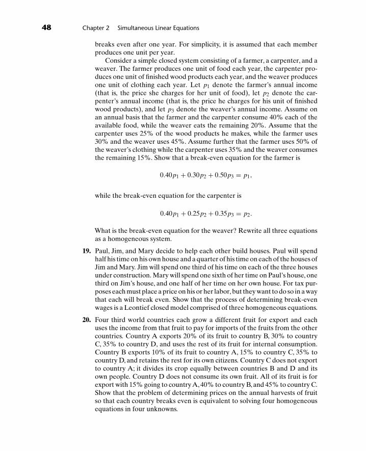
48 Chapter 2 Simultaneous Linear Equations
breaks even after one year. For simplicity, it is assumed that each memberproduces one unit per year.
Consider a simple closed system consisting of a farmer, a carpenter, and aweaver. The farmer produces one unit of food each year, the carpenter pro-duces one unit of finished wood products each year, and the weaver producesone unit of clothing each year. Let p1 denote the farmer’s annual income(that is, the price she charges for her unit of food), let p2 denote the car-penter’s annual income (that is, the price he charges for his unit of finishedwood products), and let p3 denote the weaver’s annual income. Assume onan annual basis that the farmer and the carpenter consume 40% each of theavailable food, while the weaver eats the remaining 20%. Assume that thecarpenter uses 25% of the wood products he makes, while the farmer uses30% and the weaver uses 45%. Assume further that the farmer uses 50% ofthe weaver’s clothing while the carpenter uses 35% and the weaver consumesthe remaining 15%. Show that a break-even equation for the farmer is
0.40p1 + 0.30p2 + 0.50p3 = p1,
while the break-even equation for the carpenter is
0.40p1 + 0.25p2 + 0.35p3 = p2.
What is the break-even equation for the weaver? Rewrite all three equationsas a homogeneous system.
19. Paul, Jim, and Mary decide to help each other build houses. Paul will spendhalf his time on his own house and a quarter of his time on each of the houses ofJim and Mary. Jim will spend one third of his time on each of the three housesunder construction. Mary will spend one sixth of her time on Paul’s house, onethird on Jim’s house, and one half of her time on her own house. For tax pur-poses each must place a price on his or her labor, but they want to do so in a waythat each will break even. Show that the process of determining break-evenwages is a Leontief closed model comprised of three homogeneous equations.
20. Four third world countries each grow a different fruit for export and eachuses the income from that fruit to pay for imports of the fruits from the othercountries. Country A exports 20% of its fruit to country B, 30% to countryC, 35% to country D, and uses the rest of its fruit for internal consumption.Country B exports 10% of its fruit to country A, 15% to country C, 35% tocountry D, and retains the rest for its own citizens. Country C does not exportto country A; it divides its crop equally between countries B and D and itsown people. Country D does not consume its own fruit. All of its fruit is forexport with 15% going to country A, 40% to country B, and 45% to country C.Show that the problem of determining prices on the annual harvests of fruitso that each country breaks even is equivalent to solving four homogeneousequations in four unknowns.

2.1 Linear Systems 49
21. (Leontief Input–Output Models) Consider an economy consisting of N sec-tors, with each producing goods or services unique to that sector. Let xi denotethe amount produced by the ith sector, measured in dollars. Thus xi representsthe dollar value of the supply of product i available in the economy. Assumethat every sector in the economy has a demand for a proportion (which maybe zero) of the output of every other sector. Thus, each sector j has a demand,measured in dollars, for the item produced in sector i. Let aij denote the pro-portion of item j’s revenues that must be committed to the purchase of itemsfrom sector i in order for sector j to produce its goods or services. Assumealso that there is an external demand, denoted by di and measured in dollars,for each item produced in the economy.
The problem is to determine how much of each item should be pro-duced to meet external demand without creating a surplus of any item. Showthat for a two sector economy, the solution to this problem is given by thesupply/demand equations
supply demandx1 = a11x1 + a12x2 + d1,
x2 = a21x1 + a22x2 + d2.
Show that this system is equivalent to the matrix equations
x = Ax + d and (I − A)x = d.
In this formulation, A is called the consumption matrix and d the demandvector.
22. Determine A and d in the previous problem if sector 1 must expend half of itsrevenues purchasing goods from its own sector and one third of its revenuespurchasing goods from the other sector, while sector 2 must expend one quar-ter of its revenues purchasing items from sector 1 and requires nothing fromitself. In addition, the demand for items from these two sectors are $20,000and $30,000, respectively.
23. A small town has three primary industries, coal mining (sector 1), transporta-tion (sector 2), and electricity (sector 3). Production of one dollar of coalrequires the purchase of 10 cents of electricity and 20 cents of transportation.Production of one dollar of transportation requires the purchase of 2 cents ofcoal and 35 cents of electricity. Production of one unit of electricity requiresthe purchase of 10 cents of electricity, 50 cents of coal, and 30 cents of trans-portation. The town has external contracts for $50,000 of coal, $80,000 oftransportation, and $30,000 units of electricity. Show that the problem ofdetermining how much coal, electricity, and transportation is required to sup-ply the external demand without a surplus is equivalent to solving a Leontiefinput–output model. What are A and d?
24. An economy consists of four sectors: energy, tourism, transportation, andconstruction. Each dollar of income from energy requires the expenditure

50 Chapter 2 Simultaneous Linear Equations
of 20 cents on energy costs, 10 cents on transportation, and 30 cents on con-struction. Each dollar of income gotten by the tourism sector requires theexpenditure of 20 cents on tourism (primarily in the form of complimentaryfacilities for favored customers), 15 cents on energy, 5 cents on transporta-tion, and 30 cents on construction. Each dollar of income from transportationrequires the expenditure of 40 cents on energy and 10 cents on construction;while each dollar of income from construction requires the expenditure of 5cents on construction, 25 cents on energy, and 10 cents on transportation. Theonly external demand is for tourism, and this amounts to $5 million dollars ayear. Show that the problem of determining how much energy, tourism, trans-portation, and construction is required to supply the external demand withouta surplus is equivalent to solving a Leontief input–output model. What are Aand d?
25. A constraint is often imposed on each column of the consumption matrix ofa Leontief input–output model, that the sum of the elements in each columnbe less than unity. Show that this guarantees that each sector in the economyis profitable.
2.2 Solutions by Substitution
Most readers have probably encountered simultaneous equations in high schoolalgebra. At that time, matrices were not available; hence other methods weredeveloped to solve these systems, in particular, the method of substitution. Wereview this method in this section. In the next section, we develop its matrixequivalent, which is slightly more efficient and, more importantly, better suitedfor computer implementations.
Consider the system given by (1):
a11x1 + a12x2 + · · · + a1nxn = b1,
a21x1 + a22x2 + · · · + a2nxn = b2,...
am1x1 + am2x2 + · · · + amnxn = bm.
The method of substitution is the following: take the first equation and solve forx1 in terms of x2, x3, . . . , xn and then substitute this value of x1 into all the otherequations, thus eliminating it from those equations. (If x1 does not appear in thefirst equation, rearrange the equations so that it does. For example, one mighthave to interchange the order of the first and second equations.) This new set ofequations is called the first derived set. Working with the first derived set, solvethe second equation for x2 in terms of x3, x4, . . . , xn and then substitute this valueof x2 into the third, fourth, etc. equations, thus eliminating it. This new set is the

2.2 Solutions by Substitution 51
second derived set. This process is kept up until the following set of equations isobtained:
x1 = c12x2 +c13x3 + c14x4 + · · · + c1nxn + d1,
x2 = c23x3 + c24x4 + · · · + c2nxn + d2,
x3 = c34x4 + · · · + c3nxn + d3,
...
xm = cm,m+1xm+1 + · · · + cmnxn + dm,
(6)
where the cij’s and the di’s are some combination of the original aij’s and bi’s.System (6) can be quickly solved by back substitution.
Example 1 Use the method of substitution to solve the system
r + 2s + t = 3,
2r + 3s − t = −6,
3r − 2s − 4t = −2.
Solution By solving the first equation for r and then substituting it into thesecond and third equations, we obtain the first derived set
r = 3 − 2s − t,
−s − 3t = −12,
−8s − 7t = −11.
By solving the second equation for s and then substituting it into the third equation,we obtain the second derived set
r = 3 − 2s − t,
s = 12 − 3t,
17t = 85.
By solving for t in the third equation and then substituting it into the remainingequations (of which there are none), we obtain the third derived set
r = 3 − 2s − t,
s = 12 − 3t,
t = 5.
Thus, the solution is t = 5, s = −3, r = 4. �

52 Chapter 2 Simultaneous Linear Equations
Example 2 Use the method of substitution to solve the system
x + y + 3z = −1,
2x − 2y − z = 1,
5x + y + 8z = −2.
Solution The first derived set is
x = −1 − y − 3z,
−4y − 7z = 3,
−4y − 7z = 3.
The second derived set is
x = −1 − y − 3z,
y = −34
− 74z,
0 = 0.
Since the third equation can not be solved for z, this is as far as we can go. Thus, sincewe can not obtain a unique value for z, the first and second equations will not yield aunique value for x and y. Caution:The third equation does not imply that z = 0. Onthe contrary, this equation says nothing at all about z, consequently z is completelyarbitrary. The second equation gives y in terms of z. Substituting this value intothe first equation, we obtain x in terms of z. The solution therefore is x = − 1
4 − 54z
and y = − 34 − 7
4z, z is arbitrary. Thus there are infinitely many solutions to theabove system. However, once z is chosen, x and y are determined. If z is chosento be −1, then x = y = 1, while if z is chosen to be 3, then x = −4, y = −6. Thesolutions can be expressed in the vector form
⎡⎣x
y
z
⎤⎦ =
⎡⎢⎣− 1
4 − 54z
− 34 − 7
4z
z
⎤⎥⎦ =
⎡⎢⎣− 1
4
− 340
⎤⎥⎦+ z
⎡⎢⎣− 5
4
− 741
⎤⎥⎦. �
Example 3 Use the method of substitution to solve
a + 2b − 3c + d = 1,
2a + 6b + 4c + 2d = 8.

2.2 Solutions by Substitution 53
Solution The first derived set is
a = 1 − 2b + 3c − d,
2b + 10c = 6.
The second derived set is
a = 1 − 2b + 3c − d
b = 3 − 5c
Again, since there are no more equations, this is as far as we can go, and sincethere are no defining equations for c and d, these two unknowns must be arbitrary.Solving fora andb in terms of c andd, we obtain the solutiona = −5 + 13c − d, b =3 − 5c; c and d are arbitrary. The solutions can be expressed in the vector form
⎡⎢⎢⎣
a
b
c
d
⎤⎥⎥⎦ =
⎡⎢⎢⎣
−5 + 13c − d
3 − 5c
c
d
⎤⎥⎥⎦ =
⎡⎢⎢⎣
−5300
⎤⎥⎥⎦+
⎡⎢⎢⎣
13−5
10
⎤⎥⎥⎦+ d
⎡⎢⎢⎣
−1001
⎤⎥⎥⎦.
Note that while c and d are arbitrary, once they are given a particular value, a andb are automatically determined. For example, if c is chosen as −1 and d as 4, asolution is a = −22, b = 8, c = −1, d = 4, while if c is chosen as 0 and d as −3, asolution is a = −2, b = 3, c = 0, d = −3. �
Example 4 Use the method of substitution to solve the following system:
x + 3y = 4,
2x − y = 1,
3x + 2y = 5,
5x + 15y = 20.
Solution The first derived set is
x = 4 − 3y,
−7y = −7,
−7y = −7,
0 = 0.
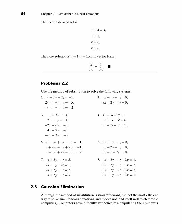
54 Chapter 2 Simultaneous Linear Equations
The second derived set is
x = 4 − 3y,
y = 1,
0 = 0,
0 = 0.
Thus, the solution is y = 1, x = 1, or in vector form[x
y
]=[
11
]. �
Problems 2.2
Use the method of substitution to solve the following systems:
1. x + 2y − 2z = −1,
2x + y + z = 5,
−x + y − z = −2.
2. x + y − z = 0,
3x + 2y + 4z = 0.
3. x + 3y = 4,
2x − y = 1,
−2x − 6y = −8,
4x − 9y = −5,
−6x + 3y = −3.
4. 4r − 3s + 2t = 1,
r + s − 3t = 4,
5r − 2s − t = 5.
5. 2l − m + n − p = 1,
l + 2m − n + 2p = −1,
l − 3m + 2n − 3p = 2.
6. 2x + y − z = 0,
x + 2y + z = 0,
3x − y + 2z = 0.
7. x + 2y − z = 5,
2x − y + 2z = 1,
2x + 2y − z = 7,
x + 2y + z = 3.
8. x + 2y + z − 2w = 1,
2x + 2y − z − w = 3,
2x − 2y + 2z + 3w = 3,
3x + y − 2z − 3w = 1.
2.3 Gaussian Elimination
Although the method of substitution is straightforward, it is not the most efficientway to solve simultaneous equations, and it does not lend itself well to electroniccomputing. Computers have difficulty symbolically manipulating the unknowns

2.3 Gaussian Elimination 55
in algebraic equations. A striking feature of the method of substitution, however,is that the unknowns remain unaltered throughout the process: x remains x, y
remains y, z remains z. Only the coefficients of the unknowns and the numbers onthe right side of the equations change from one derived set to the next. Thus, wecan save a good deal of writing, and develop a useful representation for computerprocessing, if we direct our attention to just the numbers themselves.
Definition 1 Given the system Ax = b, the augmented matrix, designated byAb, is a matrix obtained from A by adding to it one extra column, namely b.
Thus, if
A =[
1 2 34 5 6
]and b =
[78
],
then
Ab =[
1 2 3 74 5 6 8
],
while if
A =⎡⎣1 2 3
4 5 67 8 9
⎤⎦ and b =
⎡⎣−1
−2−3
⎤⎦,
then
Ab =⎡⎣1 2 3 −1
4 5 6 −27 8 9 −3
⎤⎦.
In particular, the system
x + y − 2z = −3,
2x + 5y + 3z = 11,
−x + 3y + z = 5.
has the matrix representation
⎡⎣ 1 1 −2
2 5 3−1 3 1
⎤⎦⎡⎣x
y
z
⎤⎦⎡⎣−3
115
⎤⎦,

56 Chapter 2 Simultaneous Linear Equations
with an augmented matrix of
Ab =⎡⎣ 1 1 −2 −3
2 5 3 11−1 3 1 5
⎤⎦.
Example 1 Write the set of equations in x, y, and z associated with theaugmented matrix
Ab =[−2 1 3 8
0 4 5 −3
].
Solution
−2x+ y + 3z = 8,
4y + 5z = −3.�
A second striking feature to the method of substitution is that every derived setis different from the system that preceded it. The method continues creating newderived sets until it has one that is particularly easy to solve by back-substitution.Of course, there is no purpose in solving any derived set, regardless how easy itis, unless we are assured beforehand that it has the same solution as the originalsystem. Three elementary operations that alter equations but do not change theirsolutions are:
(i) Interchange the positions of any two equations.
(ii) Multiply an equation by a nonzero scalar.
(iii) Add to one equation a scalar times another equation.
If we restate these operations in words appropriate to an augmented matrix,we obtain the elementary row operations:
(E1) Interchange any two rows in a matrix.
(E2) Multiply any row of a matrix by a nonzero scalar.
(E3) Add to one row of a matrix a scalar times another row of that same matrix.
Gaussian elimination is a matrix method for solving simultaneous linear equa-tions. The augmented matrix for the system is created, and then it is transformedinto a row-reduced matrix (see Section 1.4) using elementary row operations. Thisis most often accomplished by using operation (E3) with each diagonal elementin a matrix to create zeros in all columns directly below it, beginning with thefirst column and moving successively through the matrix, column by column. Thesystem of equations associated with a row-reduced matrix can be solved easily byback-substitution, if we solve each equation for the first unknown that appears init. This is the unknown associated with the first nonzero element in each nonzerorow of the final augmented matrix.

2.3 Gaussian Elimination 57
Example 2 Use Gaussian elimination to solve
x + 3y = 4,
2x − y = 1,
3x + 2y = 5,
5x + 15y = 20.
Solution The augmented matrix for this system is
⎡⎢⎢⎣
1 3 42 −1 13 2 55 15 20
⎤⎥⎥⎦.
Then,
⎡⎢⎢⎣
1 3 42 −1 13 2 55 15 20
⎤⎥⎥⎦→
⎡⎢⎢⎣
1 3 40 −7 −73 2 55 15 20
⎤⎥⎥⎦
⎧⎨⎩
by adding to thesecond row (−2) timesthe first row
→
⎡⎢⎢⎣
1 3 40 −7 −70 −7 −75 15 20
⎤⎥⎥⎦
⎧⎨⎩
by adding to thethird row (−3) timesthe first row
→
⎡⎢⎢⎣
1 3 40 −7 −70 −7 −70 0 0
⎤⎥⎥⎦
⎧⎨⎩
by adding to thefourth row (−5) timesthe first row
→
⎡⎢⎢⎣
1 3 40 1 10 −7 −70 0 0
⎤⎥⎥⎦
{by multiplying the
second row by−17
→
⎡⎢⎢⎣
1 3 40 1 10 0 00 0 0
⎤⎥⎥⎦.
⎧⎨⎩
by adding to thesecond row (7) timesthe first row
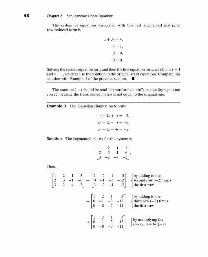
58 Chapter 2 Simultaneous Linear Equations
The system of equations associated with this last augmented matrix inrow-reduced form is
x + 3y = 4,
y = 1,
0 = 0,
0 = 0.
Solving the second equation for y and then the first equation for x, we obtain x = 1and y = 1, which is also the solution to the original set of equations. Compare thissolution with Example 4 of the previous section. �
The notation (→) should be read “is transformed into”; an equality sign is notcorrect because the transformed matrix is not equal to the original one.
Example 3 Use Gaussian elimination to solve
r + 2s + t = 3,
2r + 3s − t = −6,
3r − 2s − 4t = −2.
Solution The augmented matrix for this system is
⎡⎣1 2 1 3
2 3 −1 −63 −2 −4 −2
⎤⎦.
Then,⎡⎣1 2 1 3
2 3 −1 −63 −2 −4 −2
⎤⎦→
⎡⎣1 2 1 3
0 −1 −3 −123 −2 −4 −2
⎤⎦
⎧⎨⎩
by adding to thesecond row (−2) timesthe first row
→⎡⎣1 2 1 3
0 −1 −3 −120 −8 −7 −11
⎤⎦
⎧⎨⎩
by adding to thethird row (−3) timesthe first row
→⎡⎣1 2 1 3
0 1 3 120 −8 −7 −11
⎤⎦ {
by multiplying thesecond row by (−1)
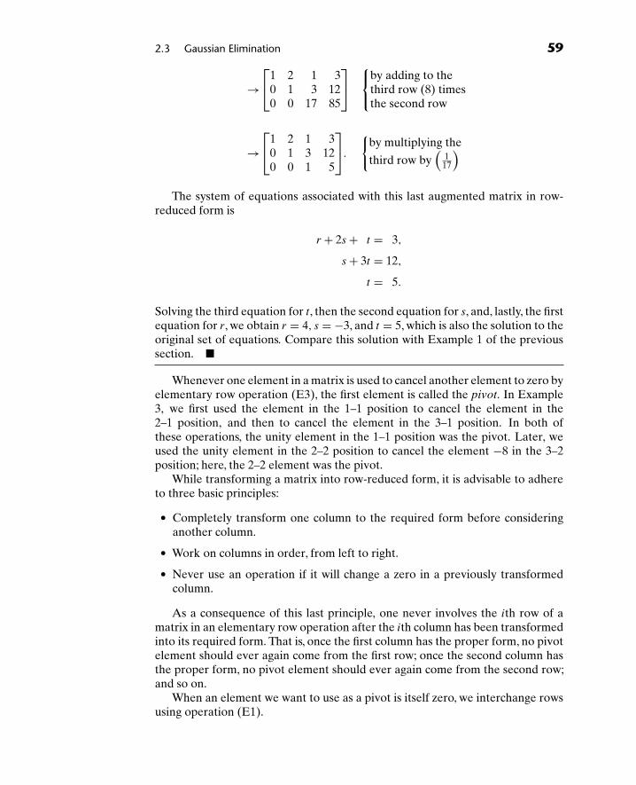
2.3 Gaussian Elimination 59
→⎡⎣1 2 1 3
0 1 3 120 0 17 85
⎤⎦
⎧⎨⎩
by adding to thethird row (8) timesthe second row
→⎡⎣1 2 1 3
0 1 3 120 0 1 5
⎤⎦.
{by multiplying the
third row by(
117
)
The system of equations associated with this last augmented matrix in row-reduced form is
r + 2s + t = 3,
s + 3t = 12,
t = 5.
Solving the third equation for t, then the second equation for s, and, lastly, the firstequation for r, we obtain r = 4, s = −3, and t = 5, which is also the solution to theoriginal set of equations. Compare this solution with Example 1 of the previoussection. �
Whenever one element in a matrix is used to cancel another element to zero byelementary row operation (E3), the first element is called the pivot. In Example3, we first used the element in the 1–1 position to cancel the element in the2–1 position, and then to cancel the element in the 3–1 position. In both ofthese operations, the unity element in the 1–1 position was the pivot. Later, weused the unity element in the 2–2 position to cancel the element −8 in the 3–2position; here, the 2–2 element was the pivot.
While transforming a matrix into row-reduced form, it is advisable to adhereto three basic principles:
● Completely transform one column to the required form before consideringanother column.
● Work on columns in order, from left to right.
● Never use an operation if it will change a zero in a previously transformedcolumn.
As a consequence of this last principle, one never involves the ith row of amatrix in an elementary row operation after the ith column has been transformedinto its required form. That is, once the first column has the proper form, no pivotelement should ever again come from the first row; once the second column hasthe proper form, no pivot element should ever again come from the second row;and so on.
When an element we want to use as a pivot is itself zero, we interchange rowsusing operation (E1).

60 Chapter 2 Simultaneous Linear Equations
Example 4 Use Gaussian elimination to solve
2c + 3d = 4,
a + 3c + d = 2,
a + b + 2c = 0.
Solution The augmented matrix is⎡⎣0 0 2 3 4
1 0 3 1 21 1 2 0 0
⎤⎦.
Normally, we would use the element in the 1–1 position to cancel to zero thetwo elements directly below it, but we cannot because it is zero. To proceed withthe reduction process, we must interchange the first row with either of the othertwo rows. The choice is arbitrary.⎡
⎣0 0 2 3 41 0 3 1 21 1 2 0 0
⎤⎦→
⎡⎣1 0 3 1 2
0 0 2 3 41 1 2 0 0
⎤⎦
⎧⎨⎩
by interchanging thefirst row with thesecond row
→⎡⎣1 0 3 1 2
0 0 2 3 40 1 −1 −1 −2
⎤⎦.
⎧⎨⎩
by adding to thethird row (−1) timesthe first row
Next, we would like to use the element in the 2–2 position to cancel to zero theelement in the 3–2 position, but we cannot because that prospective pivot is zero.We use elementary row operation (E1) once again. The transformation yields
→⎡⎣1 0 3 1 2
0 1 −1 −1 −20 0 2 3 4
⎤⎦
⎧⎨⎩
by interchanging thesecond row with thethird row
→⎡⎣1 0 3 1 2
0 1 −1 −1 −20 0 1 1.5 2
⎤⎦.
{by multiplying thethird row by (0.5)
The system of equations associated with this last augmented matrix in row-reduced form is
a + 3c + d = 2,
b − c − d = −2,
c + 1.5d = 2.

2.3 Gaussian Elimination 61
We use the third equation to solve for c, the second equation to solve for b, andthe first equation to solve for a, because these are the unknowns associated withthe first nonzero element of each nonzero row in the final augmented matrix. Wehave no defining equation for d, so this unknown remains arbitrary. The solutionis, a = −4 + 3.5d, b = −0.5d, c = 2 − 1.5d, and d arbitrary, or in vector form
⎡⎢⎢⎣
a
b
c
d
⎤⎥⎥⎦ =
⎡⎢⎢⎣
−4 + 3.5d
−0.5d
2 − 1.5d
d
⎤⎥⎥⎦ =
⎡⎢⎢⎣
−4020
⎤⎥⎥⎦+ d
2
⎡⎢⎢⎣
7−1−3
2
⎤⎥⎥⎦.
This is also the solution to the original set of equations. �
The derived set of equations associated with a row-reduced, augmented matrixmay contain an absurd equation, such as 0 = 1. In such cases, we conclude that thederived set is inconsistent, because no values of the unknowns can simultaneouslysatisfy all the equations. In particular, it is impossible to choose values of theunknowns that will make the absurd equation true. Since the derived set has thesame solutions as the original set, it follows that the original set of equations isalso inconsistent.
Example 5 Use Gaussian elimination to solve
2x + 4y + 3z = 8,
3x − 4y − 4z = 3,
5x − z = 12.
Solution The augmented matrix for this system is
⎡⎣2 4 3 8
3 −4 −4 35 0 −1 12
⎤⎦.
Then,
⎡⎣2 4 3 8
3 −4 −4 35 0 −1 12
⎤⎦→
⎡⎣1 2 1.5 4
3 −4 −4 35 0 −1 12
⎤⎦ {
by multiplying the
first row by(
12
)
→⎡⎣1 2 1.5 4
0 −10 −8.5 −95 0 −1 12
⎤⎦
⎧⎨⎩
by adding to thesecond row (−3) timesthe first row

62 Chapter 2 Simultaneous Linear Equations
→⎡⎣1 2 1.5 4
0 −10 −8.5 −90 −10 −8.5 −8
⎤⎦
⎧⎨⎩
by adding to thethird row (−5) timesthe first row
→⎡⎣1 2 1.5 4
0 1 0.85 0.90 −10 −8.5 −8
⎤⎦ {
by multiplying the
second row by(−1
10
)
→⎡⎣1 2 1.5 4
0 1 0.85 0.90 0 0 1
⎤⎦.
⎧⎨⎩
by adding to thethird row (10) timesthe second row
The system of equations associated with this last augmented matrix in row-reduced form is
x + 2y + 1.5z = 4,
y + 0.85z = 0.9,
0 = 1.
Since no values of x, y, and z can make this last equation true, this system, as wellas the original one, has no solution. �
Finally, we note that most matrices can be transformed into a variety of row-reduced forms. If a row-reduced matrix has two nonzero rows, then a differentrow-reduced matrix is easily constructed by adding to the first row any nonzeroconstant times the second row. The equations associated with both augmentedmatrices, however, will have identical solutions.
Problems 2.3
In Problems 1 through 5, construct augmented matrices for the given systems ofequations:
1. x + 2y = −3,
3x + y = 1.
2. x + 2y − z = −1,
2x − 3y + 2z = 4.
3. a + 2b = 5,
−3a + b = 13,
4a + 3b = 0.
4. 2r + 4s = 2,
3r + 2s + t = 8,
5r − 3s + 7t = 15.
5. 2r + 3s − 4t = 12,
3r − 2s = −1,
8r − s − 4t = 10.

2.3 Gaussian Elimination 63
In Problems 6 through 11, write the set of equations associated with the givenaugmented matrix and the specified variables.
6. Ab =[
1 2 50 1 8
]variables: x and y.
7. Ab =
⎡⎣1 −2 3 10
0 1 −5 −30 0 1 4
⎤⎦ variables: x, y, and z.
8. Ab =
⎡⎣1 −3 12 40
0 1 −6 −2000 0 1 25
⎤⎦ variables: r, s, and t.
9. Ab =
⎡⎣1 3 0 −8
0 1 4 20 0 0 0
⎤⎦ variables: x, y, and z.
10. Ab =
⎡⎣1 −7 2 0
0 1 −1 00 0 0 0
⎤⎦ variables: a, b, and c.
11. Ab =
⎡⎢⎢⎣
1 −1 0 10 1 −2 20 0 1 −30 0 0 1
⎤⎥⎥⎦ variables: u, v, and w.
12. Solve the system of equations defined in Problem 6.
13. Solve the system of equations defined in Problem 7.
14. Solve the system of equations defined in Problem 8.
15. Solve the system of equations defined in Problem 9.
16. Solve the system of equations defined in Problem 10.
17. Solve the system of equations defined in Problem 11.
In Problems 18 through 24, use elementary row operations to transform the givenmatrices into row-reduced form:
18.[
1 −2 5−3 7 8
]. 19.
[4 24 202 11 −8
]. 20.
[0 −1 62 7 −5
].
21.
⎡⎣ 1 2 3 4
−1 −1 2 3−2 3 0 0
⎤⎦. 22.
⎡⎣ 0 1 −2 4
1 3 2 1−2 3 1 2
⎤⎦.

64 Chapter 2 Simultaneous Linear Equations
23.
⎡⎢⎢⎣
1 3 2 0−1 −4 3 −1
2 0 −1 32 −1 4 2
⎤⎥⎥⎦. 24.
⎡⎣ 2 3 4 6 0 10
−5 −8 15 1 3 403 3 5 4 4 20
⎤⎦.
25. Solve Problem 1. 26. Solve Problem 2.
27. Solve Problem 3. 28. Solve Problem 4.
29. Solve Problem 5.
30. Use Gaussian elimination to solve Problem 1 of Section 2.2.
31. Use Gaussian elimination to solve Problem 2 of Section 2.2.
32. Use Gaussian elimination to solve Problem 3 of Section 2.2.
33. Use Gaussian elimination to solve Problem 4 of Section 2.2.
34. Use Gaussian elimination to solve Problem 5 of Section 2.2.
35. Determine a production schedule that satisfies the requirements of themanufacturer described in Problem 12 of Section 2.1.
36. Determine a production schedule that satisfies the requirements of themanufacturer described in Problem 13 of Section 2.1.
37. Determine a production schedule that satisfies the requirements of themanufacturer described in Problem 14 of Section 2.1.
38. Determine feed blends that satisfy the nutritional requirements of the petstore described in Problem 15 of Section 2.1.
39. Determine the bonus for the company described in Problem 16 ofSection 2.1.
40. Determine the number of barrels of gasoline that the producer described inProblem 17 of Section 2.1 must manufacture to break even.
41. Determine the annual incomes of each sector of the Leontief closed modeldescribed in Problem 18 of Section 2.1.
42. Determine the wages of each person in the Leontief closed model describedin Problem 19 of Section 2.1.
43. Determine the total sales revenue for each country of the Leontief closedmodel described in Problem 20 of Section 2.1.
44. Determine the production quotas for each sector of the economy describedin Problem 22 of Section 2.1.
45. An elementary matrix is a square matrix E having the property that the productEA is the result of applying a single elementary row operation on the matrixA. Form a matrix H from the 4 × 4 identity matrix I by interchanging any tworows of I, and then compute the product HA for any 4 × 4 matrix A of your

2.4 Pivoting Strategies 65
choosing. Is H an elementary matrix? How would one construct elementarymatrices corresponding to operation (E1)?
46. Form a matrix G from the 4 × 4 identity matrix I by multiplying any one rowof I by the number 5, and then compute the product GA for any 4 × 4 matrixA of your choosing. Is G an elementary matrix? How would one constructelementary matrices corresponding to operation (E2)?
47. Form a matrix F from the 4 × 4 identity matrix I by adding to one row of Ifive times another row of I. Use any two rows of your choosing. Computethe product FA for any 4 × 4 matrix A of your choosing. Is F an elemen-tary matrix? How would one construct elementary matrices corresponding tooperation (E3)?
48. A solution procedure uniquely suited to matrix equations of the form x =Ax + d is iteration. A trial solution x(0) is proposed, and then progressivelybetter estimates x(1), x(2), x(3), . . . for the solution are obtained iterativelyfrom the formula
x(i+1) = Ax(i) + d.
The iterations terminate when two successive estimates differ by less than aprespecified acceptable tolerance.
If the system comes from a Leontief input–output model, then a reasonableinitialization is x(0) = 2d. Apply this method to the system defined by Problem22 of Section 2.1. Stop after two iterations.
49. Use the iteration method described in the previous problem to solve thesystem defined in Problem 23 of Section 2.1. In particular, find the first twoiterations by hand calculations, and then use a computer to complete theiteration process.
50. Use the iteration method described in Problem 48 to solve the system definedin Problem 24 of Section 2.1. In particular, find the first two iterationsby hand calculations, and then use a computer to complete the iterationprocess.
2.4 Pivoting Strategies
Gaussian elimination is often programmed for computer implementation. Since allcomputers round or truncate numbers to a finite number of digits (e.g., the fraction1/3 might be stored as 0.33333, but never as the infinite decimal 0.333333 . . .)roundoff error can be significant. A number of strategies have been developed tominimize the effects of such errors.
The most popular strategy is partial pivoting, which requires that a pivot ele-ment always be larger in absolute value than any element below it in the samecolumn. This is accomplished by interchanging rows whenever necessary.

66 Chapter 2 Simultaneous Linear Equations
Example 1 Use partial pivoting with Gaussian elimination to solve the system
x + 2y + 4z = 18,
2x + 12y − 2z = 9,
5x + 26y + 5z = 14.
Solution The augmented matrix for this system is⎡⎣1 2 4 18
2 12 −2 95 26 5 14
⎤⎦.
Normally, the unity element in the 1–1 position would be the pivot. With partialpivoting, we compare this prospective pivot to all elements directly below it in thesame column, and if any is larger in absolute value, as is the case here with theelement 5 in the 3–1 position, we interchange rows to bring the largest elementinto the pivot position.⎡
⎣1 2 4 182 12 −2 95 26 5 14
⎤⎦→
⎡⎣5 26 5 14
2 12 −2 91 2 4 18
⎤⎦.
{by interchanging thefirst and third rows
Then,
→⎡⎣1 5.2 1 2.8
2 12 −2 91 2 4 18
⎤⎦ {
by multiplying thefirst row by 1
5
→⎡⎣1 5.2 1 2.8
0 1.6 −4 3.41 2 4 18
⎤⎦
⎧⎨⎩
by adding to thesecond row (−2) timesthe first row
→⎡⎣1 5.2 1 2.8
0 1.6 −4 3.40 −3.2 3 15.2
⎤⎦.
⎧⎨⎩
by adding to thethird row (−1) timesthe first row
The next pivot would normally be the element 1.6 in the 2–2 position. Beforeaccepting it, however, we compare it to all elements directly below it in the samecolumn. The largest element in absolute value is the element −3.2 in the 3–2position. Therefore, we interchange rows to bring this larger element into thepivot position.
Note. We do not consider the element 5.2 in the 1–2 position, even though itis the largest element in its column. Comparisons are only made between aprospective pivot and all elements directly below it. Recall one of the three basic

2.4 Pivoting Strategies 67
principles of row-reduction: never involve the first row of matrix in a row operationafter the first column has been transformed into its required form.
→⎡⎣1 5.2 1 2.8
0 −3.2 3 15.20 1.6 −4 3.4
⎤⎦ {
by interchanging thesecond and third rows
→⎡⎣1 5.2 1 2.8
0 1 −0.9375 −4.750 1.6 −4 3.4
⎤⎦ {
by multiplying thesecond row by −1
3.2
→⎡⎣1 5.2 1 2.8
0 1 −0.9375 −4.750 0 −2.5 11
⎤⎦
⎧⎨⎩
by adding to thethird row (−1.6) timesthe second row
→⎡⎣1 5.2 1 2.8
0 1 −0.9375 −4.750 0 1 −4.4
⎤⎦ {
by multiplying thethird row by −1
2.5
The new derived set of equations is
x + 5.2y + z = 2.8,
y − 0.9375z = −4.75,
z = −4.4,
which has as its solution x = 53.35, y = −8.875, and z = −4.4. �
Scaled pivoting involves ratios. A prospective pivot is divided by the largestelement in absolute value in its row, ignoring the last column. The result is com-pared to the ratios formed by dividing every element directly below the pivot bythe largest element in absolute value in its respective row, again ignoring the lastcolumn. Of these, the element that yields the largest ratio in absolute value isdesignated as the pivot, and if that element is not already in the pivot position,then row interchanges are performed to move it there.
Example 2 Use scaled pivoting with Gaussian elimination to solve the systemgiven in Example 1.
Solution The augmented matrix for this system is
⎡⎣1 2 4 18
2 12 −2 95 26 5 14
⎤⎦.
Normally, we would use the element in the 1–1 position as the pivot. Withscaled pivoting, however, we first compare ratios between elements in the first

68 Chapter 2 Simultaneous Linear Equations
column to the largest elements in absolute value in each row, ignoring the lastcolumn. The ratios are
14
= 0.25,2
12= 0.1667, and
526
= 0.1923.
The largest ratio in absolute value corresponds to the unity element in the 1–1position, so that element remains the pivot. Transforming the first column intoreduced form, we obtain
⎡⎣1 2 4 18
0 8 −10 −270 16 −15 −76
⎤⎦.
Normally, the next pivot would be the element in the 2–2 position. Instead, weconsider the ratios
810
= 0.8 and1616
= 1,
which are obtained by dividing the pivot element and every element directly belowit by the largest element in absolute value appearing in their respective rows, ignor-ing elements in the last column. The largest ratio in absolute value corresponds tothe element 16 appearing in the 3–2 position. We move it into the pivot positionby interchanging the second and third rows. The new matrix is
⎡⎣1 2 4 18
0 16 −15 −760 8 −10 −27
⎤⎦.
Completing the row-reduction transformation, we get
⎡⎢⎣1 2 4 18
0 1 −0.9375 −4.75
0 0 1 −4.4
⎤⎥⎦.
The system of equations associated with this matrix is
x + 2y + 4z = 18,
y − 0.9375z = −4.75,
z = −4.4.
The solution is, as before, x = 53.35, y = −8.875, and z = −4.4. �
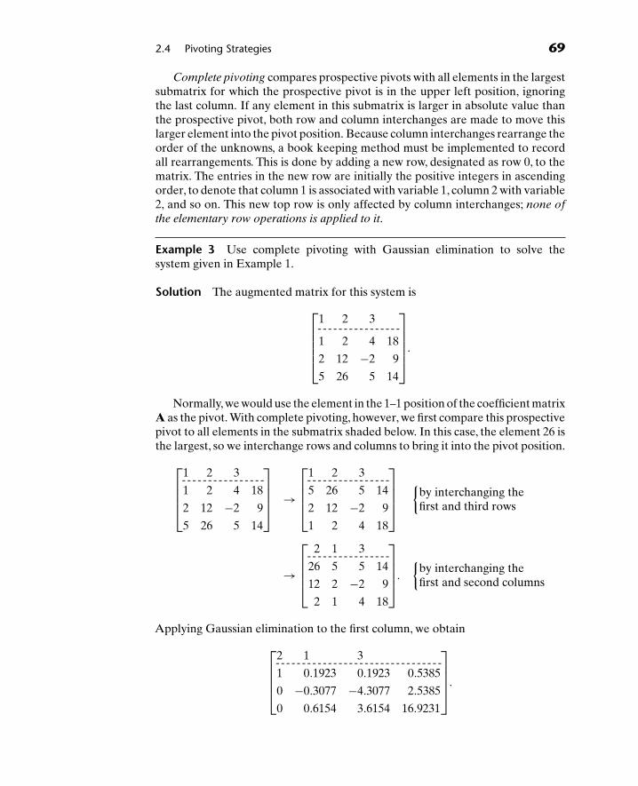
2.4 Pivoting Strategies 69
Complete pivoting compares prospective pivots with all elements in the largestsubmatrix for which the prospective pivot is in the upper left position, ignoringthe last column. If any element in this submatrix is larger in absolute value thanthe prospective pivot, both row and column interchanges are made to move thislarger element into the pivot position. Because column interchanges rearrange theorder of the unknowns, a book keeping method must be implemented to recordall rearrangements. This is done by adding a new row, designated as row 0, to thematrix. The entries in the new row are initially the positive integers in ascendingorder, to denote that column 1 is associated with variable 1, column 2 with variable2, and so on. This new top row is only affected by column interchanges; none ofthe elementary row operations is applied to it.
Example 3 Use complete pivoting with Gaussian elimination to solve thesystem given in Example 1.
Solution The augmented matrix for this system is⎡⎢⎢⎢⎢⎣
1 2 3-- - - - - - - - - - - - - - -1 2 4 18
2 12 −2 9
5 26 5 14
⎤⎥⎥⎥⎥⎦.
Normally, we would use the element in the 1–1 position of the coefficient matrixA as the pivot. With complete pivoting, however, we first compare this prospectivepivot to all elements in the submatrix shaded below. In this case, the element 26 isthe largest, so we interchange rows and columns to bring it into the pivot position.
⎡⎢⎢⎢⎣
1 2 3-- - - - - - - - - - - - - - -1 2 4 18
2 12 −2 9
5 26 5 14
⎤⎥⎥⎥⎦ →
⎡⎢⎢⎢⎣
1 2 3-- - - - - - - - - - - - - - -5 26 5 14
2 12 −2 9
1 2 4 18
⎤⎥⎥⎥⎦
{by interchanging thefirst and third rows
→
⎡⎢⎢⎢⎣
2 1 3-- - - - - - - - - - - - - - -26 5 5 14
12 2 −2 9
2 1 4 18
⎤⎥⎥⎥⎦.
{by interchanging thefirst and second columns
Applying Gaussian elimination to the first column, we obtain
⎡⎢⎢⎢⎣
2 1 3-- - - - - - - - - - - - - - - - - - - - - - - - - - - - - - -1 0.1923 0.1923 0.5385
0 −0.3077 −4.3077 2.5385
0 0.6154 3.6154 16.9231
⎤⎥⎥⎥⎦.

70 Chapter 2 Simultaneous Linear Equations
Normally, the next pivot would be −0.3077. Instead, we compare this numberin absolute value to all the numbers in the submatrix shaded above. The largestsuch element in absolute value is −4.3077, which we move into the pivot positionby interchanging the second and third column. The result is
⎡⎢⎢⎢⎣
2 3 1-- - - - - - - - - - - - - - - - - - - - - - - - - - - - - - -1 0.1923 0.1923 0.5385
0 −4.3077 −0.3077 2.5385
0 3.6154 0.6154 16.9231
⎤⎥⎥⎥⎦.
Continuing with Gaussian elimination, we obtain the row-reduced matrix
⎡⎢⎢⎢⎣
2 3 1-- - - - - - - - - - - - - - - - - - - - - - - - - - - -1 0.1923 0.1923 0.5385
0 1 0.0714 −0.5893
0 0 1 53.35
⎤⎥⎥⎥⎦.
The system associated with this matrix is
y + 0.1923z + 0.1923x = 0.5385,
z + 0.0714x = −0.5893,
x = 53.35.
Its solution is, x = 53.35, y = −8.8749, and z = −4.3985, which is within round-offerror of the answers gotten previously. �
Complete pivoting generally identifies a better pivot than scaled pivotingwhich, in turn, identifies a better pivot than partial pivoting. Nonetheless, par-tial pivoting is most often the strategy of choice. Pivoting strategies are used toavoid roundoff error. We do not need the best pivot; we only need to avoid badpivots.
Problems 2.4
In Problems 1 through 6, determine the first pivot under (a) partial pivoting,(b) scaled pivoting, and (c) complete pivoting for given augmented matrices.

2.5 Linear Independence 71
1.[
1 3 354 8 15
]. 2.
[1 −2 −55 3 85
].
3.[
1 8 153 −4 11
]. 4.
⎡⎢⎣−2 8 −3 100
4 5 4 75−3 −1 2 250
⎤⎥⎦.
5.
⎡⎢⎣1 2 3 4
5 6 7 89 10 11 12
⎤⎥⎦. 6.
⎡⎢⎣0 2 3 4 0
1 0.4 0.8 0.1 904 10 1 8 40
⎤⎥⎦.
7. Solve Problem 3 of Section 2.3 using Gaussian elimination with each of thethree pivoting strategies.
8. Solve Problem 4 of Section 2.3 using Gaussian elimination with each of thethree pivoting strategies.
9. Solve Problem 5 of Section 2.3 using Gaussian elimination with each of thethree pivoting strategies.
10. Computers internally store numbers in formats similar to the scientificnotation 0, –E–, representing the number 0. –multiplied by the power of 10signified by the digits following E. Therefore, 0.1234E06 is 123,400 while0.9935E02 is 99.35. The number of digits between the decimal point and Eis finite and fixed; it is the number of significant figures. Arithmetic opera-tions in computers are performed in registers, which have twice the numberof significant figures as storage locations.
Consider the system
0.00001x + y = 1.00001,
x + y = 2.
Show that when Gaussian elimination is implemented on this system by a computerlimited to four significant figures, the result is x = 0 and y = 1, which is incorrect.Show further that the difficulty is resolved when partial pivoting is employed.
2.5 Linear Independence
We momentarily digress from our discussion of simultaneous equations to developthe concepts of linearly independent vectors and rank of a matrix, both of whichwill prove indispensable to us in the ensuing sections.
Definition 1 A vector V1 is a linear combination of the vectors V2, V3, . . . , Vn
if there exist scalars d2, d3, . . . , dn such that
V1 = d2V2 + d3V3 + · · · + dnVn.
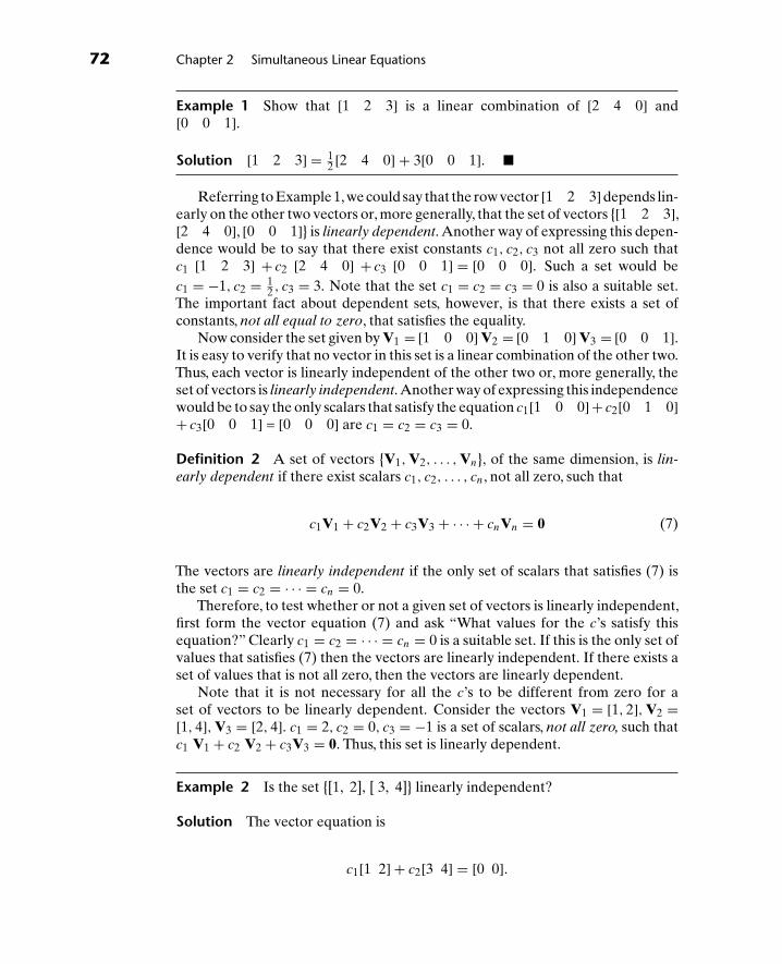
72 Chapter 2 Simultaneous Linear Equations
Example 1 Show that [1 2 3] is a linear combination of [2 4 0] and[0 0 1].
Solution [1 2 3] = 12 [2 4 0] + 3[0 0 1]. �
Referring to Example 1, we could say that the row vector [1 2 3]depends lin-early on the other two vectors or, more generally, that the set of vectors {[1 2 3],[2 4 0], [0 0 1]} is linearly dependent. Another way of expressing this depen-dence would be to say that there exist constants c1, c2, c3 not all zero such thatc1 [1 2 3] + c2 [2 4 0] + c3 [0 0 1] = [0 0 0]. Such a set would bec1 = −1, c2 = 1
2 , c3 = 3. Note that the set c1 = c2 = c3 = 0 is also a suitable set.The important fact about dependent sets, however, is that there exists a set ofconstants, not all equal to zero, that satisfies the equality.
Now consider the set given by V1 = [1 0 0] V2 = [0 1 0] V3 = [0 0 1].It is easy to verify that no vector in this set is a linear combination of the other two.Thus, each vector is linearly independent of the other two or, more generally, theset of vectors is linearly independent. Another way of expressing this independencewould be to say the only scalars that satisfy the equation c1[1 0 0]+ c2[0 1 0]+ c3[0 0 1] = [0 0 0] are c1 = c2 = c3 = 0.
Definition 2 A set of vectors {V1, V2, . . . , Vn}, of the same dimension, is lin-early dependent if there exist scalars c1, c2, . . . , cn, not all zero, such that
c1V1 + c2V2 + c3V3 + · · · + cnVn = 0 (7)
The vectors are linearly independent if the only set of scalars that satisfies (7) isthe set c1 = c2 = · · · = cn = 0.
Therefore, to test whether or not a given set of vectors is linearly independent,first form the vector equation (7) and ask “What values for the c’s satisfy thisequation?” Clearly c1 = c2 = · · · = cn = 0 is a suitable set. If this is the only set ofvalues that satisfies (7) then the vectors are linearly independent. If there exists aset of values that is not all zero, then the vectors are linearly dependent.
Note that it is not necessary for all the c’s to be different from zero for aset of vectors to be linearly dependent. Consider the vectors V1 = [1, 2], V2 =[1, 4], V3 = [2, 4]. c1 = 2, c2 = 0, c3 = −1 is a set of scalars, not all zero, such thatc1 V1 + c2 V2 + c3V3 = 0. Thus, this set is linearly dependent.
Example 2 Is the set {[1, 2], [ 3, 4]} linearly independent?
Solution The vector equation is
c1[1 2] + c2[3 4] = [0 0].

2.5 Linear Independence 73
This equation can be rewritten as
[c1 2c1] + [3c2 4c2] = [0 0]
or as
[c1 + 3c2 2c1 + 4c2] = [0 0].
Equating components, we see that this vector equation is equivalent to the system
c1 + 3c2 = 0,
2c1 + 4c2 = 0.
Using Gaussian elimination, we find that the only solution to this system is c1 =c2 = 0, hence the original set of vectors is linearly independent. �
Although we have worked exclusively with row vectors, the above definitionsare equally applicable to column vectors.
Example 3 Is the set
⎧⎨⎩⎡⎣ 2
6−2
⎤⎦,
⎡⎣3
12
⎤⎦,
⎡⎣ 8
16−3
⎤⎦⎫⎬⎭
linearly independent?
Solution Consider the vector equation
c1
⎡⎣ 2
6−2
⎤⎦+ c2
⎡⎣3
12
⎤⎦+ c3
⎡⎣ 8
16−3
⎤⎦ =
⎡⎣0
00
⎤⎦. (8)
This equation can be rewritten as
⎡⎣ 2c1
6c1−2c1
⎤⎦+
⎡⎣3c2
c22c2
⎤⎦+
⎡⎣ 8c3
16c3−3c3
⎤⎦ =
⎡⎣0
00
⎤⎦
or as ⎡⎣ 2c1 + 3c2 + 8c3
6c1 + c2 + 16c3−2c1 + 2c2 − 3c3
⎤⎦ =
⎡⎣0
00
⎤⎦.

74 Chapter 2 Simultaneous Linear Equations
By equating components, we see that this vector equation is equivalent to thesystem
2c1 + 3c2 + 8c3 = 0,
6c1 + c2 + 16c3 = 0,
−2c1 + 2c2 − 3c3 = 0.
By using Gaussian elimination, we find that the solution to this system is c1 =(− 5
2
)c3, c2 = −c3, c3 arbitrary. Thus, choosing c3 = 2, we obtain c1 = −5, c2 =
−2, c3 = 2 as a particular nonzero set of constants that satisfies (8); hence, theoriginal vectors are linearly dependent. �
Example 4 Is the set
{[12
],
[57
],
[−31
]}
linearly independent?
Solution Consider the vector equation
c1
[12
]+ c2
[57
]+ c3
[−31
]=[
00
].
This is equivalent to the system
c1 + 5c2 − 3c3 = 0,
2c1 + 7c2 + c3 = 0.
By using Gaussian elimination, we find that the solution to this system is c1 =(−26/3)c3, c2 = (7/3)c3, c3 arbitrary. Hence a particular nonzero solution is foundby choosing c3 = 3; then c1 = −26, c2 = 7, and, therefore, the vectors are linearlydependent. �
We conclude this section with a few important theorems on linear indepen-dence and dependence.
Theorem 1 A set of vectors is linearly dependent if and only if one of the vectorsis a linear combination of the others.
Proof. Let {V1, V2, . . . , Vn} be a linearly dependent set. Then there exist scalarsc1, c2, . . . , cn, not all zero, such that (7) is satisfied. Assume c1 �= 0. (Since at least

2.5 Linear Independence 75
one of the c’s must differ from zero, we lose no generality in assuming it is c1).Equation (7) can be rewritten as
c1V1 = −c2V2 − c3V3 − · · · − cnVn,
or as
V1 = −c2
c1V2 − c3
c1V3 − · · · − cn
c1Vn.
Thus, V1 is a linear combination of V2, V3, . . . , Vn. To complete the proof, wemust show that if one vector is a linear combination of the others, then the set islinearly dependent. We leave this as an exercise for the student (see Problem 36.)
OBSERVATION 1 In order for a set of vectors to be linearly dependent, it is notnecessary for every vector to be a linear combination of the others, only that thereexists one vector that is a linear combination of the others. For example, considerthe vectors [1 0], [2 0], [0 1]. Here, [0, 1] cannot be written as a linearcombination of the other two vectors; however, [2 0] can be written as a linearcombination of [1 0] and [0 1], namely, [2 0] = 2[1 0] + 0[0 1]]; hence, thevectors are linearly dependent.
Theorem 2 The set consisting of the single vector V1 is a linearly independentset if and only if V1 �= 0.
Proof. Consider the equation c1V1 = 0. If V1 �= 0, then the only way this equa-tion can be valid is if c1 = 0; hence, the set is linearly independent. If V1 = 0, thenany c1 �= 0 will satisfy the equation; hence, the set is linearly dependent.
Theorem 3 Any set of vectors that contains the zero vector is linearly dependent.
Proof. Consider the set {V1, V2, . . . , Vn, 0}. Pick c1 = c2 = · · · = cn = 0, cn+1 =5 (any other number will do). Then this is a set of scalars, not all zero, such that
c1V1 + c2V2 + · · · + cnVn + cn+10 = 0;
hence, the set of vectors is linearly dependent.
Theorem 4 If a set of vectors is linearly independent, any subset of these vectorsis also linearly independent.
Proof. See Problem 37.
Theorem 5 If a set of vectors is linearly dependent, then any larger set, containingthis set, is also linearly dependent.
Proof. See Problem 38.
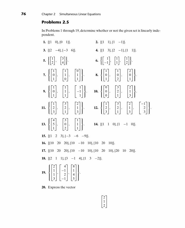
76 Chapter 2 Simultaneous Linear Equations
Problems 2.5
In Problems 1 through 19, determine whether or not the given set is linearly inde-pendent.
1. {[1 0], [0 1]}. 2. {[1 1], [1 −1]}.
3. {[2 −4], [−3 6]}. 4. {[1 3], [2 −1], [1 1]}.
5.{[
12
],[
34
]}. 6.
{[1
−1
],[
11
],[
12
]}.
7.
⎧⎨⎩⎡⎣1
01
⎤⎦,
⎡⎣1
10
⎤⎦,
⎡⎣0
11
⎤⎦⎫⎬⎭. 8.
⎧⎨⎩⎡⎣1
01
⎤⎦,
⎡⎣1
02
⎤⎦,
⎡⎣2
01
⎤⎦⎫⎬⎭.
9.
⎧⎨⎩⎡⎣1
01
⎤⎦,
⎡⎣1
11
⎤⎦,
⎡⎣ 1
−11
⎤⎦⎫⎬⎭. 10.
⎧⎨⎩⎡⎣0
00
⎤⎦,
⎡⎣3
21
⎤⎦,
⎡⎣2
13
⎤⎦⎫⎬⎭.
11.
⎧⎨⎩⎡⎣1
23
⎤⎦,
⎡⎣3
21
⎤⎦,
⎡⎣2
13
⎤⎦⎫⎬⎭. 12.
⎧⎨⎩⎡⎣1
23
⎤⎦,
⎡⎣3
21
⎤⎦,
⎡⎣2
13
⎤⎦,
⎡⎣−1
23
⎤⎦⎫⎬⎭.
13.
⎧⎨⎩⎡⎣4
51
⎤⎦,
⎡⎣3
02
⎤⎦,
⎡⎣1
11
⎤⎦⎫⎬⎭. 14. {[1 1 0], [1 −1 0]}.
15. {[1 2 3], [−3 −6 −9]}.16. {[10 20 20], [10 −10 10], [10 20 10]}.17. {[10 20 20], [10 −10 10], [10 20 10], [20 10 20]}.18. {[2 1 1], [3 −1 4], [1 3 −2]}.
19.
⎧⎪⎪⎨⎪⎪⎩⎡⎢⎢⎣
2113
⎤⎥⎥⎦,
⎡⎢⎢⎣
4−1
2−1
⎤⎥⎥⎦,
⎡⎢⎢⎣
8145
⎤⎥⎥⎦⎫⎪⎪⎬⎪⎪⎭.
20. Express the vector
⎡⎣2
12
⎤⎦

2.5 Linear Independence 77
as a linear combination of
⎧⎨⎩⎡⎣1
10
⎤⎦,
⎡⎣ 1
0−1
⎤⎦,
⎡⎣1
11
⎤⎦⎫⎬⎭.
21. Can the vector [2 3] be expressed as a linear combination of the vectorsgiven in (a) Problem 1, (b) Problem 2, or (c) Problem 3?
22. Can the vector [1 1 1]T be expressed as a linear combination of the vectorsgiven in (a) Problem 7, (b) Problem 8, or (c) Problem 9?
23. Can the vector [2 0 3]T be expressed as a linear combination of the vectorsgiven in Problem 8?
24. A set of vectors S is a spanning set for another set of vectors R if every vectorin R can be expressed as a linear combination of the vectors in S. Show thatthe vectors given in Problem 1 are a spanning set for all two-dimensional rowvectors. Hint: Show that for any arbitrary real numbers a and b, the vector[a b] can be expressed as a linear combination of the vectors in Problem 1.
25. Show that the vectors given in Problem 2 are a spanning set for all two-dimensional row vectors.
26. Show that the vectors given in Problem 3 are not a spanning set for all two-dimensional row vectors.
27. Show that the vectors given in Problem 3 are a spanning set for all vectors ofthe form [a −2a], where a designates any real number.
28. Show that the vectors given in Problem 4 are a spanning set for all two-dimensional row vectors.
29. Determine whether the vectors given in Problem 7 are a spanning set for allthree-dimensional column vectors.
30. Determine whether the vectors given in Problem 8 are a spanning set for allthree-dimensional column vectors.
31. Determine whether the vectors given in Problem 8 are a spanning set forvectors of the form [a 0 a]T, where a denotes an arbitrary real number.
32. A set of vectors S is a basis for another set of vectors R if S is a spanning setfor R and S is linearly independent. Determine which, if any, of the sets givenin Problems 1 through 4 are a basis for the set of all two dimensional rowvectors.
33. Determine which, if any, of the sets given in Problems 7 through 12 are a basisfor the set of all three dimensional column vectors.
34. Prove that the columns of the 3 × 3 identity matrix form a basis for the set ofall three dimensional column vectors.

78 Chapter 2 Simultaneous Linear Equations
35. Prove that the rows of the 4 × 4 identity matrix form a basis for the set of allfour dimensional row vectors.
36. Finish the proof of Theorem 1. (Hint: Assume that V1 can be written as alinear combination of the other vectors.)
37. Prove Theorem 4.
38. Prove Theorem 5.
39. Prove that the set of vectors {x, kx} is linearly dependent for any choice of thescalar k.
40. Prove that if x and y are linearly independent, then so too are x + y and x − y.
41. Prove that if the set {x1, x2, . . . , xn} is linearly independent then so too is theset {k1x1, k2x2, . . . , knxn} for any choice of the non-zero scalars k1, k2, . . . , kn.
42. Let A be an n × n matrix and let {x1, x2, . . . , xk} and {y1, y2, . . . , yk} be twosets of n-dimensional column vectors having the property that Axi = yi =1, 2, . . . , k. Show that the set {x1, x2, . . . , xk} is linearly independent if the set{y1, y2, . . . , yk} is.
2.6 Rank
If we interpret each row of a matrix as a row vector, the elementary row operationsare precisely the operations used to form linear combinations; namely, multiplyingvectors (rows) by scalars and adding vectors (rows) to other vectors (rows). Thisobservation allows us to develop a straightforward matrix procedure for deter-mining when a set of vectors is linearly independent. It rests on the concept ofrank.
Definition 1 The row rank of a matrix is the maximum number of linearly inde-pendent vectors that can be formed from the rows of that matrix, considering eachrow as a separate vector. Analogically, the column rank of a matrix is the maximumnumber of linearly independent columns, considering each column as a separatevector.
Row rank is particularly easy to determine for matrices in row-reduced form.
Theorem 1 The row rank of a row-reduced matrix is the number of nonzerorows in that matrix.
Proof. We must prove two facts: First, that the nonzero rows, considered asvectors, form a linearly independent set, and second, that every larger set is linearlydependent. Consider the equation
c1v1 + c2v2 + · · · + crvr = 0, (9)

2.6 Rank 79
where v1 is the first nonzero row, v2 is the second nonzero row, . . . , and vr is thelast nonzero row of a row-reduced matrix. The first nonzero element in the firstnonzero row of a row-reduced matrix must be unity. Assume it appears in columnj. Then, no other rows have a nonzero element in that column. Consequently,when the left side of Eq. (9) is computed, it will have c1 as its jth component.Since the right side of Eq. (9) is the zero vector, it follows that c1 = 0. A similarargument then shows iteratively that c2, . . . , cr, are all zero. Thus, the nonzerorows are linearly independent.
If all the rows of the matrix are nonzero, then they must comprise a maximumnumber of linearly independent vectors, because the row rank cannot be greaterthan the number of rows in the matrix. If there are zero rows in the row-reducedmatrix, then it follows from Theorem 3 of Section 2.5 that including them couldnot increase the number of linearly independent rows. Thus, the largest numberof linearly independent rows comes from including just the nonzero rows.
Example 1 Determine the row rank of the matrix
A =
⎡⎢⎢⎢⎣
1 0 −2 5 3
0 0 1 −4 1
0 0 0 1 0
0 0 0 0 0
⎤⎥⎥⎥⎦.
Solution A is in row-reduced form. Since it contains three nonzero rows, its rowrank is three. �
The following two theorems, which are proved in the Final Comments to thischapter, are fundamental.
Theorem 2 The row rank and column rank of a matrix are equal.
For any matrix A, we call this common number the rank of A and denote it byr(A).
Theorem 3 If B is obtained from A by an elementary row (or column) operation,then r(B) = r(A).
Theorems 1 through 3 suggest a useful procedure for determining the rank ofany matrix: Simply use elementary row operations to transform the given matrixto row-reduced form, and then count the number of nonzero rows.
Example 2 Determine the rank of
A =
⎡⎢⎢⎣
1 3 42 −1 13 2 55 15 20
⎤⎥⎥⎦.

80 Chapter 2 Simultaneous Linear Equations
Solution In Example 2 of Section 2.3, we transferred this matrix into the row-reduced form ⎡
⎢⎢⎣1 3 40 1 10 0 00 0 0
⎤⎥⎥⎦.
This matrix has two nonzero rows so its rank, as well as that of A, is two. �
Example 3 Determine the rank of
B =⎡⎣1 2 1 3
2 3 −1 −63 −2 −4 −2
⎤⎦.
Solution In Example 3 of Section 2.3, we transferred this matrix into the row-reduced form ⎡
⎣1 2 1 30 1 3 120 0 1 5
⎤⎦.
This matrix has three nonzero rows so its rank, as well as that of B, is three. �
A similar procedure can be used for determining whether a set of vectors islinearly independent: Form a matrix in which each row is one of the vectors in thegiven set, and then determine the rank of that matrix. If the rank equals the num-ber of vectors, the set is linearly independent; if not, the set is linearly dependent.In either case, the rank is the maximal number of linearly independent vectorsthat can be formed from the given set.
Example 4 Determine whether the set⎧⎨⎩⎡⎣ 2
6−2
⎤⎦,
⎡⎣3
12
⎤⎦,
⎡⎣ 8
16−3
⎤⎦⎫⎬⎭
is linearly independent.
Solution We consider the matrix⎡⎣2 6 −2
3 1 28 16 −3
⎤⎦.

2.6 Rank 81
Reducing this matrix to row-reduced form, we obtain⎡⎢⎣
1 3 −1
0 1 − 58
0 0 0
⎤⎥⎦.
This matrix has two nonzero rows, so its rank is two. Since this is less than thenumber of vectors in the given set, that set is linearly dependent.
We can say even more: The original set of vectors contains a subset of twolinearly independent vectors, the same number as the rank. Also, since no rowinterchanges were involved in the transformation to row-reduced form, we canconclude that the third vector is linear combination of the first two. �
Example 5 Determine whether the set
{[0 1 2 3 0], [1 3 −1 2 1],[2 6 −1 −3 1], [4 0 1 0 2]}
is linearly independent.
Solution We consider the matrix⎡⎢⎢⎢⎣
0 1 2 3 01 3 −1 2 12 6 −1 −3 14 0 1 0 2
⎤⎥⎥⎥⎦,
which can be reduced (after the first two rows are interchanged) to the row-reduced form ⎡
⎢⎢⎢⎣1 3 −1 2 10 1 2 3 00 0 1 −7 −1
0 0 0 1 27175
⎤⎥⎥⎥⎦.
This matrix has four nonzero rows, hence its rank is four, which is equal to thenumber of vectors in the given set. Therefore, the set is linearly independent. �
Example 6 Can the vector [11
]

82 Chapter 2 Simultaneous Linear Equations
be written as a linear combination of the vectors
[36
]and
[24
]?
Solution The matrix
A =[
3 62 4
]
can be transformed into the row-reduced form
[3 60 0
],
which has rank one; hence A has just one linearly independent row vector. Incontrast, the matrix
B =⎡⎣1 1
3 62 4
⎤⎦
can be transformed into the row-reduced form,
⎡⎣1 1
0 10 0
⎤⎦,
which has rank two; hence B has two linearly independent row vectors. Since Bis precisely A with one additional row, it follows that the additional row [1, 1]Tis independent of the other two and, therefore, cannot be written as a linearcombination of the other two vectors. �
We did not have to transform B in Example 6 into row-reduced form to deter-mine whether the three-vector set was linearly independent. There is a more directapproach. Since B has only two columns, its column rank must be less than or equalto two (why?). Thus, the column rank is less than three. It follows from Theorem3 that the row rank of B is less than three, so the three vectors must be linearlydependent. Generalizing this reasoning, we deduce one of the more importantresults in linear algebra.
Theorem 4 In an n-dimensional vector space, every set of n + 1 vectors is linearlydependent.

2.6 Rank 83
Problems 2.6
In Problems 1–5, find the rank of the given matrix.
1.[
1 2 03 1 −5
]. 2.
⎡⎣4 1
2 32 2
⎤⎦.
3.
⎡⎣ 1 4 −2
2 8 −4−1 −4 2
⎤⎦. 4.
⎡⎣1 2 4 2
1 1 3 21 2 4 2
⎤⎦.
5.
⎡⎣1 7 0
0 1 11 1 0
⎤⎦.
In Problems 6 through 22, use rank to determine whether the given set of vectorsis linearly independent.
6. {[1 0], [0 1]}. 7. {[1 1], [1 −1]}.
8. {[2 −4], [−3 6]}. 9. {[1 3], [2 −1], [1 1]}.
10.{[
12
],
[34
]}. 11.
{[1
−1
],
[11
],
[12
]}.
12.
⎧⎨⎩⎡⎣1
01
⎤⎦,
⎡⎣1
10
⎤⎦,
⎡⎣0
11
⎤⎦⎫⎬⎭. 13.
⎧⎨⎩⎡⎣1
01
⎤⎦,
⎡⎣1
02
⎤⎦,
⎡⎣2
01
⎤⎦⎫⎬⎭.
14.
⎧⎨⎩⎡⎣1
01
⎤⎦,
⎡⎣1
11
⎤⎦,
⎡⎣ 1
−11
⎤⎦⎫⎬⎭. 15.
⎧⎨⎩⎡⎣0
00
⎤⎦,
⎡⎣3
21
⎤⎦,
⎡⎣2
13
⎤⎦⎫⎬⎭.
16.
⎧⎨⎩⎡⎣1
23
⎤⎦,
⎡⎣3
21
⎤⎦,
⎡⎣2
13
⎤⎦⎫⎬⎭. 17.
⎧⎨⎩⎡⎣1
23
⎤⎦,
⎡⎣3
21
⎤⎦,
⎡⎣2
13
⎤⎦,
⎡⎣−1
2−3
⎤⎦⎫⎬⎭.
18. {[1 1 0], [1 −1 0]}.19. {[1 2 3], [−3 −6 −9]}.20. {[10 20 20], [10 −10 10], [10 20 10]}.21. {[10 20 20], [10 −10 10], [10 20 10], [20 10 20]}.22. {[2 1 1], [3 −1 4], [1 3 −2]}.23. Can the vector [2 3] be expressed as a linear combination of the vectors
given in (a) Problem 6, (b) Problem 7, or (c) Problem 8?

84 Chapter 2 Simultaneous Linear Equations
24. Can the vector [1 1 1]T be expressed as a linear combination of the vectorsgiven in (a) Problem 12, (b) Problem 13, or (c) Problem 14?
25. Can the vector [2 0 3]T be expressed as a linear combination of the vectorsgiven in Problem 13?
26. Can [3 7] be written as a linear combination of the vectors [1 2] and [3 2]?27. Can [3 7] be written as a linear combination of the vectors [1 2] and [4 8]?28. Find a maximal linearly independent subset of the vectors given in Problem 9.
29. Find a maximal linearly independent subset of the vectors given in Problem 13.
30. Find a maximal linearly independent subset of the set.
[1 2 4 0], [2 4 8 0], [1 −1 0 1], [4 2 8 2], [4 −1 4 3].31. What is the rank of the zero matrix?
32. Show r(AT) = r(A).
2.7 Theory of Solutions
Consider once again the system Ax = b of m equations and n unknowns given inEq. (2). Designate the n columns of A by the vectors V1, V2, . . . , Vn. Then Eq. (2)can be rewritten in the vector form
x1V1 + x2V2 + · · · + xnVn = b. (10)
Example 1 Rewrite the following system in the vector form (10):
x − 2y + 3z = 7,
4x + 5y − 6z = 8.
Solution
x
[14
]+ y
[−25
]+ z
[3
−6
]=[
78
]�
Thus, finding solutions to (1) and (2) is equivalent to finding scalarsx1, x2, . . . , xn that satisfy (10). This, however, is asking precisely the question “Isthe vector b a linear combination of V1, V2, . . . , Vn?” If b is a linear combinationof V1, V2, . . . , Vn, then there will exist scalars x1, x2, . . . , xn that satisfy (10) andthe system is consistent. If b is not a linear combination of these vectors, that is, if bis linearly independent of the vectors V1, V2, . . . , Vn, then no scalars x1, x2, . . . , xn
will exist that satisfy (10) and the system is inconsistent.Taking a hint from Example 6 of Section 2.6, we have the following theorem.

2.7 Theory of Solutions 85
Theorem 1 The system Ax = b is consistent if and only if r(A) = r(Ab).
Once a system is deemed consistent, the following theorem specifies thenumber of solutions.
Theorem 2 If the system Ax = b is consistent and r(A) = k then the solutions areexpressible in terms of n − k arbitrary unknowns (where n represents the numberof unknowns in the system).
Theorem 2 is almost obvious. To determine the rank of Ab, we must reduceit to row-reduced form. The rank is the number of nonzero rows. With Gaussianelimination, we use each nonzero row to solve for the variable associated with thefirst nonzero entry in it. Thus, each nonzero row defines one variable, and all othervariables remain arbitrary.
Example 2 Discuss the solutions of the system
x + y − z = 1,
x + y − z = 0.
Solution
A =[
1 1 −11 1 −1
], b =
[10
], Ab =
[1 1 −1 11 1 −1 0
].
Here, r(A) = 1, r(Ab) = 2. Thus, r(A) �= r(Ab) and no solution exists. �
Example 3 Discuss the solutions of the system
x + y + w = 3,
2x + 2y + 2w = 6,
−x − y − w = −3.
Solution
A =⎡⎣ 1 1 1
2 2 2−1 −1 −1
⎤⎦, b =
⎡⎣ 3
6−3
⎤⎦, Ab =
⎡⎣ 1 1 1 3
2 2 2 6−1 −1 −1 −3
⎤⎦.
Here r(A) = r(Ab) = 1; hence, the system is consistent. In this case, n = 3 andk = 1; thus, the solutions are expressible in terms of 3 − 1 = 2 arbitrary unknowns.Using Gaussian elimination, we find that the solution is x = 3 − y − w where y andw are both arbitrary. �

86 Chapter 2 Simultaneous Linear Equations
Example 4 Discuss the solutions of the system
2x − 3y + z = −1,
x − y + 2z = 2,
2x + y − 3z = 3.
Solution
A =⎡⎣2 −3 1
1 −1 22 1 −3
⎤⎦, b =
⎡⎣−1
23
⎤⎦, Ab =
⎡⎣2 −3 1 −1
1 −1 2 22 1 −3 3
⎤⎦.
Here r(A) = r(Ab) = 3, hence the system is consistent. Since n = 3 and k = 3, thesolution will be in n − k = 0 arbitrary unknowns. Thus, the solution is unique (noneof the unknowns are arbitrary) and can be obtained by Gaussian elimination asx = y = 2, z = 1. �
Example 5 Discuss the solutions of the system
x + y − 2z = 1,
2x + y + z = 2,
3x + 2y − z = 3,
4x + 2y + 2z = 4.
Solution
A =
⎡⎢⎢⎣
1 1 −22 1 13 2 −14 2 2
⎤⎥⎥⎦, b =
⎡⎢⎢⎣
1234
⎤⎥⎥⎦, Ab =
⎡⎢⎢⎣
1 1 −2 12 1 1 23 2 −1 34 2 2 4
⎤⎥⎥⎦.
Here r(A) = r(Ab) = 2. Thus, the system is consistent and the solutions will be interms of 3 − 2 = 1 arbitrary unknowns. Using Gaussian elimination, we find thatthe solution is x = 1 − 3z, y = 5z, and z is arbitrary. �
In a consistent system, the solution is unique if k = n. If k �= n, the solution willbe in terms of arbitrary unknowns. Since these arbitrary unknowns can be chosento be any constants whatsoever, it follows that there will be an infinite number ofsolutions. Thus, a consistent system will possess exactly one solution or an infinitenumber of solutions; there is no inbetween.

2.7 Theory of Solutions 87
A homogeneous system of simultaneous linear equations has the form
a11x1 + a12x2 + · · · + a1nxn = 0,
a21x1 + a22x2 + · · · + a2nxn = 0,...
am1x1 + am2x2 + · · · + amnxn = 0,
(11)
or the matrix form
Ax = 0. (12)
Since Eq. (12) is a special case of Eq. (2) with b = 0, all the theory developedfor the system Ax = b remains valid. Because of the simplified structure of ahomogeneous system, one can draw conclusions about it that are not valid for anonhomogeneous system. For instance, a homogeneous system is always consis-tent. To verify this statement, note that x1 = x2 = · · · = xn = 0 is always a solutionto Eq. (12). Such a solution is called the trivial solution. It is, in general, the non-trivial solutions (solutions in which one or more of the unknowns is different fromzero) that are of the greatest interest.
It follows from Theorem 2, that if the rank of A is less than n(n being thenumber of unknowns), then the solution will be in terms of arbitrary unknowns.Since these arbitrary unknowns can be assigned nonzero values, it follows thatnontrivial solutions exist. On the other hand, if the rank of A equals n, then thesolution will be unique, and, hence, must be the trivial solution (why?). Thus, itfollows that:
Theorem 3 The homogeneous system (12) will admit nontrivial solutions if andonly if r(A) �= n.
Problems 2.7
In Problems 1–9, discuss the solutions of the given system in terms of consistencyand number of solutions. Check your answers by solving the systems whereverpossible.
1. x − 2y = 0,
x + y = 1,
2x − y = 1.
2. x + y = 0,
2x − 2y = 1,
x − y = 0.
3. x + y + z = 1,
x − y + z = 2,
3x + y + 3z = 4.
4. x + 3y + 2z − w = 2,
2x − y + z + w = 3.

88 Chapter 2 Simultaneous Linear Equations
5. 2x − y + z = 0,
x + 2y − z = 4,
x + y + z = 1.
6. 2x + 3y = 0,
x − 4y = 0,
7. x − y + 2z = 0,
2x + 3y − z = 0,
−2x + 7y − 7z = 0.
8. x − y + 2z = 0,
2x − 3y − z = 0,
−2x + 7y − 9z = 0.
9. x − 2y + 3z + 3w = 0,
y − 2z + 2w = 0,
x + y − 3z + 9w = 0.
2.8 Final Comments on Chapter 2
We would like to show that the column rank of a matrix equals its row rank, andthat an elementary row operation of any kind does not alter the rank.
Lemma 1 If B is obtained from A by interchanging two columns of A, then bothA and B have the same column rank.
Proof. The set of vectors formed from the columns of A is identical to the setformed from the columns of B, and, therefore, the two matrices must have thesame column rank.
Lemma 2 If Ax = 0 and Bx = 0 have the same set of solutions, then the columnrank of A is less than or equal to the column rank of B.
Proof. Let the order of A be m × n. Then, the system Ax = 0 is a set of m
equations in the n unknowns x1, x2, . . . , xn, which has the vector form
x1A1 + x2A2 + · · · + xnAn = 0, (13)
where A1, A2, . . . , An denote the columns of A. Similarly, the system Bx = 0 hasthe vector form
x1B1 + x2B2 + · · · + xnBn = 0. (14)
We shall assume that the column rank of A is greater than the column rank of Band show that this assumption leads to a contradiction. It will then follow that thereverse must be true, which is precisely what we want to prove.
Denote the column rank of A as a and the column rank of B as b. We assumethat a > b. Since the column rank of A is a, there must exist a columns of A that

2.8 Final Comments 89
are linearly independent. If these columns are not the first a columns, rearrangethe order of the columns so they are. Lemma 1 guarantees such reorderings donot alter the column rank. Thus, A1, A2, . . . , Aa are linearly independent. Sincea is assumed greater than b, we know that the first a columns of B are not lin-early independent. Since they are linearly dependent, there must exist constantsc1, c2, . . . , ca — not all zero — such that
c1B1 + c2B2 + · · · + caBa = 0.
It then follows that
c1B1 + c2B2 + · · · + caBa + 0Ba+1 + · · · + 0Bn = 0,
from which we conclude that
x1 = c1, x2 = c2, . . . , xa = ca, xa+1 = 0, . . . , xn = 0.
is a solution of Eq. (14). Since every solution to Eq. (14) is also a solution to Eq.(12), we have
c1A1 + c2A2 + · · · + caAa + 0Aa+1 + · · · + 0An = 0,
or more simply
c1A1 + c2A2 + · · · + caAa = 0,
where all the c’s are not all zero. But this implies that the first a columns of Aare linearly dependent, which is a contradiction of the assumption that they werelinearly independent.
Lemma 3 If Ax = 0 and Bx = 0 have the same set of solutions, then A and Bhave the same column rank.
Proof. If follows from Lemma 2 that the column rank of A is less than or equalto the column rank of B. By reversing the roles of A and B, we can also concludefrom Lemma 2 that the column rank of B is less than or equal to the column rankof A. As a result, the two column ranks must be equal.
Theorem 1 An elementary row operation does not alter the column rank of amatrix.
Proof. Denote the original matrix as A, and let B denote a matrix obtainedby applying an elementary row operation to A; and consider the two homoge-neous systems Ax = 0 and Bx = 0. Since elementary row operations do not altersolutions, both of these systems have the same solution set. Theorem 1 followsimmediately from Lemma 3.

90 Chapter 2 Simultaneous Linear Equations
Lemma 4 The column rank of a matrix is less than or equal to its row rank.
Proof. Denote rows of A by A1, A2, . . . Am, the column rank of matrix A by c
and its row rank by r. There must exist r rows of A which are linearly independent.If these rows are not the first r rows, rearrange the order of the rows so they are.Theorem 1 guarantees such reorderings do not alter the column rank, and theycertainly do not alter the row rank. Thus, A1, A2, . . . , Ar are linearly independent.Define partitioned matrices R and S by
R =
⎡⎢⎢⎢⎣
A1A2...
Ar
⎤⎥⎥⎥⎦ and S =
⎡⎢⎢⎢⎣
Ar+1Ar+2
...
An
⎤⎥⎥⎥⎦.
Then A has the partitioned form
A =[
RS
].
Every row of S is a linear combination of the rows of R. Therefore, there existconstants tij such that
Ar+1 = tr+1,1A1 + tr+1,2A2 + · · · + tr+1,rAr,
Ar+2 = tr+2,1A1 + tr+2,2A2 + · · · + tr+2,rAr,
...
An = tn,1A1 + tn,2A2 + · · · + tn,rAr,
which may be written in the matrix form
S = TR,
where
T =
⎡⎢⎢⎢⎣
tr+1,1 tr+1,2 · · · tr+1,n
tr+2,1 tr+2,2 · · · tr+2,n...
......
...
tn,1 tn,2 · · · tn,n
⎤⎥⎥⎥⎦.
Then, for any n-dimensional vector x, we have
Ax =[
RS
]x =
[RxSx
]=[
RxTRx
].

2.8 Final Comments 91
Thus, Ax = 0 if and only if Rx = 0. It follows from Lemma 3 that both A and Rhave the same column rank. But the columns of R are r-dimensional vectors, soits column rank cannot be larger than r. Thus,
c = column rank of A = column rank of R ≤ r = row rank of A
Lemma 5 The row rank of a matrix is less than or equal to its column rank.
Proof. By applying Lemma 4 to AT, we conclude that the column rank of AT isless than or equal to the row rank of AT. But since the columns of AT are the rowsof A and vice-versa, the result follows immediately.
Theorem 2 The row rank of a matrix equals its column rank.
Proof. The result is immediate from Lemmas 4 and 5.
Theorem 3 An elementary row operation does not alter the row rank of a matrix.
Proof. This theorem is an immediate consequence of both Theorems 1 and 2.

This page intentionally left blank

33The Inverse
3.1 Introduction
Definition 1 An inverse of an n × n matrix A is a n × n matrix B having theproperty that
AB = BA = I. (1)
Here, B is called an inverse of A and is usually denoted by A−1. If a squarematrix A has an inverse, it is said to be invertible or nonsingular. If A does notpossess an inverse, it is said to be singular. Note that inverses are only definedfor square matrices. In particular, the identity matrix is invertible and is its owninverse because
II = I.
Example 1 Determine whether
B =[
1 12
13
14
]or C =
[−2 132 − 1
2
]
are inverses for
A =[
1 23 4
].
Solution B is an inverse if and only if AB = BA = I; C is an inverse if and onlyif AC = CA = I. Here,
AB =[
1 2
3 4
][1 1
213
14
]=[
53 1
133
52
]�=[
1 0
0 1
],
93

94 Chapter 3 The Inverse
while
AC =[
1 2
3 4
][−2 132 − 1
2
]=[
1 0
0 1
]=[−2 1
32 − 1
2
][1 2
3 4
]= CA.
Thus, B is not an inverse for A, but C is. We may write A−1 = C. �
Definition 1 is a test for checking whether a given matrix is an inverse of anothergiven matrix. In the Final Comments to this chapter we prove that if AB = I fortwo square matrices of the same order, then A and B commute, and BA = I. Thus,we can reduce the checking procedure by half. A matrix B is an inverse for a squarematrix A if either AB = I or BA = I; each equality automatically guarantees theother for square matrices. We will show in Section 3.4 that an inverse is unique. Ifa square matrix has an inverse, it has only one.
Definition 1 does not provide a method for finding inverses. We develop sucha procedure in the next section. Still, inverses for some matrices can be founddirectly.
The inverse for a diagonal matrix D having only nonzero elements on its maindiagonal is also a diagonal matrix whose diagonal elements are the reciprocals ofthe corresponding diagonal elements of D. That is, if
D =
⎡⎢⎢⎢⎢⎢⎣
λ1 0λ2
λ3. . .
0 λn
⎤⎥⎥⎥⎥⎥⎦,
then
D−1 =
⎡⎢⎢⎢⎢⎢⎢⎢⎢⎢⎢⎢⎢⎣
1λ1
0
1λ2
1λ3
. . .
01λn
⎤⎥⎥⎥⎥⎥⎥⎥⎥⎥⎥⎥⎥⎦
.
It is easy to show that if any diagonal element in a diagonal matrix is zero, thenthat matrix is singular. (See Problem 57.)
An elementary matrix E is a square matrix that generates an elementary rowoperation on a matrix A (which need not be square) under the multiplicationEA. Elementary, matrices are constructed by applying the desired elementaryrow operation to an identity matrix of appropriate order. The appropriate order

3.1 Introduction 95
for both I and E is a square matrix having as many columns as there are rowsin A; then, the multiplication EA is defined. Because identity matrices containmany zeros, the process for constructing elementary matrices can be simplifiedstill further. After all, nothing is accomplished by interchanging the positions ofzeros, multiplying zeros by nonzero constants, or adding zeros to zeros.
(i) To construct an elementary matrix that interchanges the ith row with the jthrow, begin with an identity matrix of the appropriate order. First, interchangethe unity element in the i − i position with the zero in the j − i position, andthen interchange the unity element in the j − j position with the zero in thei − j position.
(ii) To construct an elementary matrix that multiplies the ith row of a matrix bythe nonzero scalar k, replace the unity element in the i − i position of theidentity matrix of appropriate order with the scalar k.
(iii) To construct an elementary matrix that adds to the jth row of a matrix k timesthe ith row, replace the zero element in the j − i position of the identity matrixof appropriate order with the scalar k.
Example 2 Find elementary matrices that when multiplied on the right by any4 × 3 matrix A will (a) interchange the second and fourth rows of A, (b) multiplythe third row of A by 3, and (c) add to the fourth row of A − 5 times its second row.
Solution
(a)
⎡⎢⎢⎣
1 0 0 00 0 0 10 0 1 00 1 0 0
⎤⎥⎥⎦, (b)
⎡⎢⎢⎣
1 0 0 00 1 0 00 0 3 00 0 0 1
⎤⎥⎥⎦, (c)
⎡⎢⎢⎣
1 0 0 00 1 0 00 0 1 00 −5 0 1
⎤⎥⎥⎦. �
Example 3 Find elementary matrices that when multiplied on the right by any3 × 5 matrix A will (a) interchange the first and second rows of A, (b) multiply thethird row of A by −0.5, and (c) add to the third row of A − 1 times its second row.
Solution
(a)
⎡⎣0 1 0
1 0 00 0 1
⎤⎦, (b)
⎡⎣1 0 0
0 1 00 0 −0.5
⎤⎦, (c)
⎡⎣1 0 0
0 1 00 −1 1
⎤⎦. �
The inverse of an elementary matrix that interchanges two rows is the matrixitself, it is its own inverse. The inverse of an elementary matrix that multipliesone row by a nonzero scalar k is gotten by replacing k by 1/k. The inverse of

96 Chapter 3 The Inverse
an elementary matrix which adds to one row a constant k times another row isobtained by replacing the scalar k by −k.
Example 4 Compute the inverses of the elementary matrices found inExample 2.
Solution
(a)
⎡⎢⎢⎢⎣
1 0 0 0
0 0 0 1
0 0 1 0
0 1 0 0
⎤⎥⎥⎥⎦, (b)
⎡⎢⎢⎢⎣
1 0 0 0
0 1 0 0
0 0 13 0
0 0 0 1
⎤⎥⎥⎥⎦, (c)
⎡⎢⎢⎢⎣
1 0 0 0
0 1 0 0
0 0 1 0
0 5 0 1
⎤⎥⎥⎥⎦. �
Example 5 Compute the inverses of the elementary matrices found inExample 3.
Solution
(a)
⎡⎢⎣0 1 0
1 0 00 0 1
⎤⎥⎦, (b)
⎡⎢⎣1 0 0
0 1 00 0 −2
⎤⎥⎦, (c)
⎡⎢⎣1 0 0
0 1 00 1 1
⎤⎥⎦.
Finally, if A can be partitioned into the block diagonal form,
A =
⎡⎢⎢⎢⎢⎢⎢⎣
A1 0A2
A3
. . .
0 An
⎤⎥⎥⎥⎥⎥⎥⎦,
then A is invertible if and only if each of the diagonal blocks A1, A2, . . . , An isinvertible and
A−1 =
⎡⎢⎢⎢⎢⎢⎢⎢⎢⎣
A−11 0
A−12
A−13
. . .
0 A−1n
⎤⎥⎥⎥⎥⎥⎥⎥⎥⎦
. �

3.1 Introduction 97
Example 6 Find the inverse of
A =
⎡⎢⎢⎢⎢⎢⎢⎢⎢⎢⎣
2 0 0 0 0 0 00 5 0 0 0 0 00 0 1 0 0 0 00 0 4 1 0 0 00 0 0 0 1 0 00 0 0 0 0 0 10 0 0 0 0 1 0
⎤⎥⎥⎥⎥⎥⎥⎥⎥⎥⎦
.
Solution Set
A1 =[
2 00 5
], A2 =
[1 04 1
], and A3 =
⎡⎣1 0 0
0 0 10 1 0
⎤⎦;
then, A is in the block diagonal form
A =⎡⎢⎣A1 0
A20 A3
⎤⎥⎦.
Here A1 is a diagonal matrix with nonzero diagonal elements, A2 is an elementarymatrix that adds to the second row four times the first row, and A3 is an elementarymatrix that interchanges the second and third rows; thus
A−11 =
[12 0
0 15
], A−1
2 =[
1 0−4 1
], and A−1
3 =⎡⎣1 0 0
0 0 10 1 0
⎤⎦,
and
A−1 =
⎡⎢⎢⎢⎢⎢⎢⎢⎢⎢⎢⎣
12 0 0 0 0 0 0
0 15 0 0 0 0 0
0 0 1 0 0 0 00 0 −4 1 0 0 00 0 0 0 1 0 00 0 0 0 0 0 10 0 0 0 0 1 0
⎤⎥⎥⎥⎥⎥⎥⎥⎥⎥⎥⎦
. �

98 Chapter 3 The Inverse
Problems 3.1
1. Determine if any of the following matrices are inverses for
A =[
1 32 9
]:
(a)
⎡⎣1 1
3
12
19
⎤⎦, (b)
[−1 −3−2 −9
],
(c)
[3 −1
− 23
13
], (d)
[9 −3
−2 1
].
2. Determine if any of the following matrices are inverses for
B =[
1 11 1
]:
(a)
[1 11 1
], (b)
[−1 11 −1
],
(c)[
1 1−1 −1
], (d)
[2 −1
−1 2
].
3. Calculate directly the inverse of
A =[
8 25 3
].
Hint: Define
B =[a b
c d
].
Calculate AB, set the product equal to I, and then solve for the elements of B.
4. Use the procedure described in Problem 3 to calculate the inverse of
C =[
1 22 1
].
5. Use the procedure described in Problem 3 to calculate the inverse of
D =[
1 11 1
].

3.1 Introduction 99
6. Show directly that the inverse of
A =[a b
c d
]
when ad − bc �= 0 is
A−1 = 1ad − bc
[d −b
−c a
].
7. Use the results of Problem 6 to calculate the inverse of[1 13 4
].
8. Use the results of Problem 6 to calculate the inverse of[2 14 3
].
9. Use the results of Problem 6 to calculate the inverse of[1 1
212
13
].
10. Use the results of Problem 6 to calculate the inverse of[10 2030 40
].
In Problems 11 through 26, find elementary matrices that when multiplied on theright by a matrix A will generate the specified result.
11. Interchange the order of the first and second row of the 2 × 2 matrix A.
12. Multiply the first row of a 2 × 2 matrix A by three.
13. Multiply the second row of a 2 × 2 matrix A by −5.
14. Multiply the second row of a 3 × 3 matrix A by −5.
15. Add to the second row of a 2 × 2 matrix A three times its first row.
16. Add to the first row of a 2 × 2 matrix A three times its second row.
17. Add to the second row of a 3 × 3 matrix A three times its third row.
18. Add to the third row of a 3 × 4 matrix A five times its first row.
19. Add to the second row of a 4 × 4 matrix A eight times its fourth row.
20. Add to the fourth row of a 5 × 7 matrix A −2 times its first row.
21. Interchange the second and fourth rows of a 4 × 6 matrix A.

100 Chapter 3 The Inverse
22. Interchange the second and fourth rows of a 4 × 4 matrix A.
23. Interchange the second and fourth rows of a 6 × 6 matrix A.
24. Multiply the second row of a 2 × 5 matrix A by seven.
25. Multiply the third row of a 5 × 2 matrix A by seven.
26. Multiply the second row of a 3 × 5 matrix A by −0.2.
In Problems 27 through 42, find the inverses of the given elementary matrices.
27.[
2 00 1
], 28.
[1 20 1
], 29.
[1 0
−3 1
], 30.
[1 01 1
],
31.
⎡⎣1 0 0
0 2 00 0 1
⎤⎦, 32.
⎡⎣0 1 0
1 0 00 0 1
⎤⎦, 33.
⎡⎣1 0 0
0 1 03 0 1
⎤⎦,
34.
⎡⎣1 0 3
0 1 00 0 1
⎤⎦, 35.
⎡⎣1 0 0
0 1 −20 0 1
⎤⎦, 36.
⎡⎣1 0 0
0 1 00 0 −4
⎤⎦,
37.
⎡⎢⎢⎣
1 0 0 00 1 0 00 0 0 10 0 1 0
⎤⎥⎥⎦, 38.
⎡⎢⎢⎣
1 0 0 00 1 0 70 0 1 00 0 0 1
⎤⎥⎥⎦, 39.
⎡⎢⎢⎣
1 0 0 00 1 0 0
−3 0 1 00 0 0 1
⎤⎥⎥⎦,
40.
⎡⎢⎢⎣
0 0 0 10 1 0 00 0 1 01 0 0 0
⎤⎥⎥⎦, 41.
⎡⎢⎢⎣
1 0 0 00 1 0 00 1 1 00 0 0 1
⎤⎥⎥⎦, 42.
⎡⎢⎢⎣
1 0 0 00 1 0 0
0 0 − 12 0
0 0 0 1
⎤⎥⎥⎦,
In Problems 43 through 55, find the inverses, if they exist, of the given diagonal orblock diagonal matrices.
43.[
2 00 3
], 44.
[−1 00 0
], 45.
[3 00 −3
], 46.
[12 0
0 − 23
],
47.
⎡⎣10 0 0
0 5 00 0 5
⎤⎦, 48.
⎡⎣1 1 0
0 1 00 0 −1
⎤⎦, 49.
⎡⎣−4 0 0
0 −2 00 0 3
5
⎤⎦,
50.
⎡⎢⎢⎣
1 2 0 00 1 0 00 0 1 00 0 2 1
⎤⎥⎥⎦, 51.
⎡⎢⎢⎣
2 0 0 00 3 0 00 0 1 −30 0 0 1
⎤⎥⎥⎦, 52.
⎡⎢⎢⎣
4 0 0 00 5 0 00 0 6 00 0 0 1
⎤⎥⎥⎦,

3.2 Calculating Inverses 101
53.
⎡⎢⎢⎢⎣
0 1 0 01 0 0 00 0 0 10 0 1 0
⎤⎥⎥⎥⎦, 54.
⎡⎢⎢⎢⎣
0 0 1 00 1 0 01 0 0 00 0 0 7
⎤⎥⎥⎥⎦, 55.
⎡⎢⎢⎢⎣
4 0 0 00 5 0 00 0 1 60 0 0 1
⎤⎥⎥⎥⎦,
56. Prove that a square zero matrix does not have an inverse.
57. Prove that if a diagonal matrix has at least one zero on its main diagonal, thenthat matrix cannot have an inverse.
58. Prove that if A2 = I, then A−1 = A.
3.2 Calculating Inverses
In Section 2.3, we developed a method for transforming any matrix into row-reduced form using elementary row operations. If we now restrict our attentionto square matrices, we may say that the resulting row-reduced matrices are uppertriangular matrices having either a unity or zero element in each entry on themain diagonal. This provides a simple test for determining which matrices haveinverses.
Theorem 1 A square matrix has an inverse if and only if reduction to row-reduced form by elementary row operations results in a matrix having all unityelements on the main diagonal.
We shall prove this theorem in the Final Comments to this chapter as
Theorem 2 An n × n matrix has an inverse if and only if it has rank n.
Theorem 1 not only provides a test for determining when a matrix is invertible,but it also suggests a technique for obtaining the inverse when it exists. Once amatrix has been transformed to a row-reduced matrix with unity elements on themain diagonal, it is a simple matter to reduce it still further to the identity matrix.This is done by applying elementary row operation (E3)—adding to one row ofa matrix a scalar times another row of the same matrix—to each column of thematrix, beginning with the last column and moving sequentially toward the firstcolumn, placing zeros in all positions above the diagonal elements.
Example 1 Use elementary row operations to transform the upper triangularmatrix
A =⎡⎣1 2 1
0 1 30 0 1
⎤⎦
to the identity matrix.

102 Chapter 3 The Inverse
Solution ⎡⎣1 2 1
0 1 30 0 1
⎤⎦→
⎡⎣1 2 1
0 1 00 0 1
⎤⎦
⎧⎨⎩
by adding tothe second row (−3)
times the third row
→⎡⎣1 2 0
0 1 00 0 1
⎤⎦
⎧⎨⎩
by adding tothe first row (−1)
times the third row
→⎡⎣1 0 0
0 1 00 0 1
⎤⎦
⎧⎨⎩
by adding tothe first row (−2)
times the second row�
To summarize, we now know that a square matrix A has an inverse if and onlyif it can be transformed into the identity matrix by elementary row operations.Moreover, it follows from the previous section that each elementary row operationis represented by an elementary matrix E that generates the row operation underthe multiplication EA. Therefore, A has an inverse if and only if there exist asequence of elementary matrices. E1, E2, . . . , Ek such that
EkEk−1 · · · E3 E2 E1 A = I.
But, if we denote the product of these elementary matrices as B, we then haveBA = I, which implies that B = A−1. That is, the inverse of a square matrix A offull rank is the product of those elementary matrices that reduce A to the identitymatrix! Thus, to calculate the inverse of A, we need only keep a record of theelementary row operations, or equivalently the elementary matrices, that wereused to reduce A to I. This is accomplished by simultaneously applying the sameelementary row operations to both A and an identity matrix of the same order,because if
Ek Ek−1 · · · E3 E2 E1 A = I,
then
(Ek Ek−1 · · · E3 E2 E1)I = Ek Ek−1 · · · E3 E2 E1 = A−1.
We have, therefore, the following procedure for calculating inverses when theyexist. Let A be the n × n matrix we wish to invert. Place next to it another n × n
matrix B which is initially the identity. Using elementary row operations on A,transform it into the identity. Each time an operation is performed on A, repeatthe exact same operation on B. After A is transformed into the identity, the matrixobtained from transforming B will be A−1.
If A cannot be transformed into an indentity matrix, which is equivalent tosaying that its row-reduced from contains at least one zero row, then A does nothave an inverse.

3.2 Calculating Inverses 103
Example 2 Invert
A =[
1 23 4
].
Solution
[1 23 4
∣∣∣∣ 1 00 1
]→[
1 20 −2
∣∣∣∣ 1 0−3 1
] ⎧⎨⎩
by adding tothe second row (−3)
times the first row
→[
1 2
0 1
∣∣∣∣∣ 1 032 − 1
2
].
{by multiplyingthe second row by (− 1
2 )
A has been transformed into row-reduced form with a main diagonal of only unityelements; it has an inverse. Continuing with transformation process, we get
→[
1 0
0 1
∣∣∣∣∣ −2 132 − 1
2
].
⎧⎨⎩
by adding tothe first row (−2)
times the second row
Thus,
A−1 =[−2 1
32 − 1
2
]. �
Example 3 Find the inverse of
A =⎡⎣5 8 1
0 2 14 3 −1
⎤⎦.
Solution⎡⎣5 8 1
0 2 14 3 −1
∣∣∣∣∣∣1 0 00 1 00 0 1
⎤⎦→
⎡⎣1 1.6 0.2
0 2 14 3 −1
∣∣∣∣∣∣0.2 0 00 1 00 0 1
⎤⎦ {
by multiplying thefirst row by (0.2)
→⎡⎣1 1.6 0.2
0 2 10 −3.4 −1.8
∣∣∣∣∣∣0.2 0 00 1 0
−0.8 0 1
⎤⎦⎧⎨⎩
by adding to thethird row (−4)
times the first row

104 Chapter 3 The Inverse
→⎡⎣1 1.6 0.2
0 1 0.50 −3.4 −1.8
∣∣∣∣∣∣0.2 0 00 0.5 0
−0.8 0 1
⎤⎦ {
by multiplying thesecond row by (0.5)
→⎡⎣1 1.6 0.2
0 1 0.50 0 −0.1
∣∣∣∣∣∣0.2 0 00 0.5 0
−0.8 1.7 1
⎤⎦
⎧⎨⎩
by adding to thethird row (3.4)
times the second row
→⎡⎣1 1.6 0.2
0 1 0.50 0 1
∣∣∣∣∣∣0.2 0 00 0.5 08 −17 −10
⎤⎦.
{by multiplying thethird row by (−0.1)
A has been transformed into row-reduced form with a main diagonal of only unityelements; it has an inverse. Continuing with the transformation process, we get
→⎡⎣1 1.6 0.2
0 1 00 0 1
∣∣∣∣∣∣0.2 0 0
−4 9 58 −17 −10
⎤⎦
⎧⎨⎩
by adding to thesecond row (−0.5)
times the third row
→⎡⎣1 1.6 0
0 1 00 0 1
∣∣∣∣∣∣−1.4 3.4 2−4 9 5
8 −17 −10
⎤⎦
⎧⎨⎩
by adding to thefirst row (−0.2)
times the third row
→⎡⎣1 0 0
0 1 00 0 1
∣∣∣∣∣∣5 −11 −6
−4 9 58 −17 −10
⎤⎦.
⎧⎨⎩
by adding to thefirst row (−1.6)
times the second row
Thus,
A−1 =⎡⎣ 5 −11 −6
−4 9 58 −17 −10
⎤⎦. �
Example 4 Find the inverse of
A =⎡⎣0 1 1
1 1 11 1 3
⎤⎦.
Solution⎡⎣0 1 1
1 1 11 1 3
∣∣∣∣∣∣1 0 00 1 00 0 1
⎤⎦ →
⎡⎣1 1 1
0 1 11 1 3
∣∣∣∣∣∣0 1 01 0 00 0 1
⎤⎦ {
by interchanging thefirst and second rows

3.2 Calculating Inverses 105
→⎡⎣1 1 1
0 1 10 0 2
∣∣∣∣∣∣0 1 01 0 00 −1 1
⎤⎦
⎧⎨⎩
by adding to thethe third row (−1)
times the first row
→⎡⎢⎣1 1 1
0 1 10 0 1
∣∣∣∣∣∣∣0 1 01 0 0
0 − 12
12
⎤⎥⎦ {
by multiplying thethird row by ( 1
2 )
→⎡⎢⎣1 1 1
0 1 00 0 1
∣∣∣∣∣∣∣0 1 01 1
2 − 12
0 − 12
12
⎤⎥⎦
⎧⎨⎩
by adding to thesecond row (−1)
times the third row
→
⎡⎢⎢⎣
1 1 0
0 1 0
0 0 1
∣∣∣∣∣∣∣∣0 3
2 − 12
1 12 − 1
2
0 − 12
12
⎤⎥⎥⎦
⎧⎨⎩
by adding to thefirst row (−1)
times the third row
→⎡⎢⎣1 0 0
0 1 00 0 1
∣∣∣∣∣∣∣−1 1 0
1 12 − 1
2
0 − 12
12
⎤⎥⎦.
⎧⎨⎩
by adding to thefirst row (−1)
times the second row
Thus,
A−1 =⎡⎢⎣
−1 1 0
1 12 − 1
2
0 − 12
12
⎤⎥⎦. �
Example 5 Invert
A =[
1 2
2 4
].
Solution
[1 22 4
∣∣∣∣ 1 00 1
]→[
1 20 0
∣∣∣∣ 1 0−2 1
].
⎧⎨⎩
by adding tothe second row (−2)
times the first row
A has been transformed into row-reduced form. Since the main diagonal containsa zero element, here in the 2–2 position, the matrix A does not have an inverse. Itis singular. �

106 Chapter 3 The Inverse
Problems 3.2
In Problems 1–20, find the inverses of the given matrices, if they exist.
1.[
1 13 4
], 2.
[2 11 2
], 3.
[4 44 4
],
4.[
2 −13 4
], 5.
[8 35 2
], 6.
[1 1
212
13
],
7.
⎡⎣1 1 0
1 0 10 1 1
⎤⎦, 8.
⎡⎣0 0 1
1 0 00 1 0
⎤⎦, 9.
⎡⎣2 0 −1
0 1 23 1 1
⎤⎦,
10.
⎡⎣1 2 3
4 5 67 8 9
⎤⎦, 11.
⎡⎣2 0 0
5 1 04 1 1
⎤⎦, 12.
⎡⎣2 1 5
0 3 −10 0 2
⎤⎦,
13.
⎡⎣3 2 1
4 0 13 9 2
⎤⎦, 14.
⎡⎣ 1 2 −1
2 0 1−1 1 3
⎤⎦, 15.
⎡⎣1 2 1
3 −2 −42 3 −1
⎤⎦,
16.
⎡⎣2 4 3
3 −4 −45 0 −1
⎤⎦, 17.
⎡⎣5 0 −1
2 −1 22 3 −1
⎤⎦, 18.
⎡⎣3 1 1
1 3 −12 3 −1
⎤⎦,
19.
⎡⎢⎢⎣
1 1 1 20 1 −1 10 0 2 30 0 0 −2
⎤⎥⎥⎦, 20.
⎡⎢⎢⎣
1 0 0 02 −1 0 04 6 2 03 2 4 −1
⎤⎥⎥⎦.
21. Use the results of Problems 11 and 20 to deduce a theorem involving inversesof lower triangular matrices.
22. Use the results of Problems 12 and 19 to deduce a theorem involving theinverses of upper triangular matrices.
23. Matrix inversion can be used to encode and decode sensitive messages fortransmission. Initially, each letter in the alphabet is assigned a unique positiveinteger, with the simplest correspondence being
A B C D E F G H I J K L M N O P Q R S T U V W X Y Z↓ ↓ ↓ ↓ ↓ ↓ ↓ ↓ ↓ ↓ ↓ ↓ ↓ ↓ ↓ ↓ ↓ ↓ ↓ ↓ ↓ ↓ ↓ ↓ ↓ ↓1 2 3 4 5 6 7 8 9 10 11 12 13 14 15 16 17 18 19 20 21 22 23 24 25 26
.

3.2 Calculating Inverses 107
Zeros are used to separate words. Thus, the message
SHE IS A SEER
is encoded
19 8 5 0 9 19 0 1 0 19 5 5 18 0.
This scheme is too easy to decipher, however, so a scrambling effect is addedprior to transmission. One scheme is to package the coded string as a set of2-tuples, multiply each 2-tuple by a 2 × 2 invertible matrix, and then transmitthe new string. For example, using the matrix
A =[
1 2
2 3
],
the coded message above would be scrambled into
[1 2
2 3
][19
8
]=[
35
62
],
[1 2
2 3
][5
0
]=[
5
10
],
[1 2
2 3
][9
19
]=[
47
75
], etc.,
and the scrambled message becomes
35 62 5 10 47 75 . . . .
Note an immediate benefit from the scrambling: the letter S, which was orig-inally always coded as 19 in each of its three occurrences, is now coded as a35 the first time and as 75 the second time. Continue with the scrambling, anddetermine the final code for transmitting the above message.
24. Scramble the message SHE IS A SEER using, matrix
A =[
2 −34 5
].
25. Scramble the message AARON IS A NAME using the matrix and stepsdescribed in Problem 23.

108 Chapter 3 The Inverse
26. Transmitted messages are unscrambled by again packaging the received mes-sage into 2-tuples and multiplying each vector by the inverse of A. To decodethe scrambled message
18 31 44 72
using the encoding scheme described in Problem 23, we first calculate
A−1 =[−3 2
2 −1
],
and then
[−3 22 −1
][1831
]=[
85
],
[−3 22 −1
][4472
]=[
1216
].
The unscrambled message is
8 5 12 16
which, according to the letter-integer correspondence given in Problem 23,translates to HELP. Using the same procedure, decode the scrambled message
26 43 40 60 18 31 28 51.
27. Use the decoding procedure described in Problem 26, but with the matrix Agiven in Problem 24, to decipher the transmitted message
16 120 −39 131 −27 45 38 76 −51 129 28 56.
28. Scramble the message SHE IS A SEER by packaging the coded letters into3-tuples and then multiplying by the 3 × 3 invertible matrix
A =⎡⎢⎣1 0 1
0 1 11 1 0
⎤⎥⎦.
Add as many zeros as necessary to the end of the message to generate complete3-tuples.

3.3 Simultaneous Equations 109
3.3 Simultaneous Equations
One use of the inverse is in the solution of systems of simultaneous linearequations. Recall, from Section 1.3 that any such system may be written in the form
Ax = b, (2)
where A is the coefficient matrix, b is a known vector, and x is the unknown vectorwe wish to find. If A is invertible, then we can premultiply (2) by A−1 and obtain
A−1Ax = A−1b.
But A−1A = 1, therefore
Ix = A−1b
or
x = A−1b. (3)
Hence, (3) shows that if A is invertible, then x can be obtained by premultiplyingb by the inverse of A.
Example 1 Solve the following system for x and y:
x − 2y = −9,
−3x + y = 2.
Solution Define
A =[
1 −2−3 1
], x =
[x
y
], b =
[−92
];
then the system can be written as Ax = b, hence x = A−1b. Using the methodgiven in Section 3.2 we find that
A−1 =(− 1
5
) [1 23 1
].
Thus, [x
y
]= x = A−1b =
(− 1
5
) [1 23 1
][−92
]=(− 1
5
) [ −5−25
]=[
15
].
Using the definition of matrix equality (two matrices are equal if and only if theircorresponding elements are equal), we have that x = 1 and y = 5. �
110 Chapter 3 The Inverse
Example 2 Solve the following system for x, y, and z:
5x + 8y + z = 2,
2y + z = −1,
4x + 3y − z = 3.
Solution
A =⎡⎣5 8 1
0 2 14 3 −1
⎤⎦, x =
⎡⎣x
y
z
⎤⎦, b =
⎡⎣ 2
−13
⎤⎦.
A−1 is found to be (see Example 3 of Section 3.2)⎡⎣ 5 −11 −6
−4 9 58 −17 −10
⎤⎦.
Thus, ⎡⎣x
y
z
⎤⎦ = x = A−1b =
⎡⎣ 5 −11 −6
−4 9 58 −17 −10
⎤⎦⎡⎣ 2
−13
⎤⎦ =
⎡⎣ 3
−23
⎤⎦,
hence x = 3, y = −2, and z = 3. �
Not only does the invertibility of A provide us with a solution of the systemAx = b, it also provides us with a means of showing that this solution is unique(that is, there is no other solution to the system).
Theorem 1 If A is invertible, then the system of simultaneous linear equationsgiven by Ax = b has one and only one solution.
Proof. Define w = A−1b. Since we have already shown that w is a solution toAx = b, it follows that
Aw = b. (4)
Assume that there exists another solution y. Since y is a solution, we have that
Ay = b. (5)
Equations (4) and (5) imply that
Aw = Ay. (6)

3.3 Simultaneous Equations 111
Premultiply both sides of (6) by A−1. Then
A−1Aw = A−1Ay,
Iw = Iy,
or
w = y.
Thus, we see that if y is assumed to be a solution of Ax = b, it must, in fact, equalw. Therefore, w = A−1b is the only solution to the problem.
If A is singular, so that A−1 does not exist, then (3) is not valid and othermethods, such as Gaussian elimination, must be used to solve the given system ofsimultaneous equations.
Problems 3.3
In Problems 1 through 12, use matrix inversion, if possible, to solve the givensystems of equations:
1. 2.x + 2y = −3,
3x + y = 1.
a + 2b = 5,
−3a + b = 13.
3. 4.4x + 2y = 6,
2x − 3y = 7.
4l − p = 1,
5l − 2p = −1.
5. 6.2x + 3y = 8,
6x + 9y = 24.
x + 2y − z = −1,
2x + 3y + 2z = 5,
y − z = 2.
7. 8.2x + 3y − z = 4,
−x − 2y + z = −2,
3x − y = 2.
60l + 30m + 20n = 0,
30l + 20m + 15n = −10,
20l + 15m + 12n = −10.
9. 10.2r + 4s = 2,
3r + 2s + t = 8,
5r − 3s + 7t = 15.
2r + 4s = 3,
3r + 2s + t = 8,
5r − 3s + 7t = 15.
11. 12.2r + 3s − 4t = 12,
3r − 2s = −1,
8r − s − 4t = 10.
x + 2y − 2z = −1,
2x + y + z = 5,
−x + y − z = −2.
13. Use matrix inversion to determine a production schedule that satisfies therequirements of the manufacturer described in Problem 12 of Section 2.1.

112 Chapter 3 The Inverse
14. Use matrix inversion to determine a production schedule that satisfies therequirements of the manufacturer described in Problem 13 of Section 2.1.
15. Use matrix inversion to determine a production schedule that satisfies therequirements of the manufacturer described in Problem 14 of Section 2.1.
16. Use matrix inversion to determine the bonus for the company described inProblem 16 of Section 2.1.
17. Use matrix inversion to determine the number of barrels of gasoline that theproducer described in Problem 17 of Section 2.1 must manufacture to breakeven.
18. Use matrix inversion to solve the Leontief input–output model described inProblem 22 of Section 2.1.
19. Use matrix inversion to solve the Leontief input–output model described inProblem 23 of Section 2.1.
3.4 Properties of the Inverse
Theorem 1 If A, B, and C are square matrices of the same order with AB = Iand CA = I, then B = C.
Proof. C = CI = C(AB) = (CA)B = IB = B.
Theorem 2 The inverse of a matrix is unique.
Proof. Suppose that B and C are inverse of A. Then, by (1), we have that
AB = I, BA = I, AC = I, and CA = I.
It follows from Theorem 1 that B = C. Thus, if B and C are both inverses of A,they must in fact be equal. Hence, the inverse is unique.
Using Theorem 2, we can prove some useful properties of the inverse of amatrix A when A is nonsingular.
Property 1(A−1)−1 = A.
Proof. See Problem 1.
Property 2 (AB)−1 = B−1A−1.
Proof. (AB)−1 denotes the inverse of AB. However,(B−1A−1) (AB) =
B−1 (A−1A)
B = B−1IB = B−1B = I. Thus, B−1A−1 is also an inverse for AB,and, by uniqueness of the inverse, B−1A−1 = (AB)−1.
Property 3 (A1A2 · · · An)−1 = A−1
n A−1n−1 · · · A−1
2 A−11 .

3.4 Properties of the Inverse 113
Proof. This is an extension of Property 2 and, as such, is proved in a similarmanner.
CAUTION. Note that Property 3 states that the inverse of a product is not theproduct of the inverses but rather the product of the inverses commuted.
Property 4(AT)−1 = (A−1)T
Proof.(AT)−1
denotes the inverse of AT. However, using the property of thetranspose that (AB)T = BTAT, we have that
(AT)(A−1)T = (A−1A
)T = IT = I.
Thus,(A−1)T is an inverse of AT, and by uniqueness of the inverse,
(A−1)T =(
AT)−1.
Property 5 (λA)−1 = (1/λ) (A)−1 if λ is a nonzero scalar.
Proof. (λA)−1 denotes the inverse of λA. However,
(λA)(1/λ)A−1 = λ(1/λ)AA−1 = 1·I = I.
Thus, (1/λ)A−1 is an inverse of λA, and by uniqueness of the inverse (1/λ)A−1 =(λA)−1.
Property 6 The inverse of a nonsingular symmetric matrix is symmetric.
Proof. See Problem 18.
Property 7 The inverse of a nonsingular upper or lower triangular matrix isagain an upper or lower triangular matrix respectively.
Proof. This is immediate from Theorem 2 and the constructive proceduredescribed in Section 3.2 for calculating inverses.
Finally, the inverse provides us with a straightforward way of defining squarematrices raised to negative integral powers. If A is nonsingular then we defineA−n = (A−1)n.
Example 1 Find A−2 if
A =⎡⎣ 1
312
12 1
⎤⎦.

114 Chapter 3 The Inverse
Solution
A−2 =(
A−1)2
=[
12 −6−6 4
]2
=[
12 −6−6 4
][12 −6−6 4
]=[
180 −96−96 52
]. �
Problems 3.4
1. Prove Property 1.
2. Verify Property 2 for
A =[
1 12 3
]and B =
[2 51 2
].
3. Verify Property 2 for
A =[
1 23 4
]and B =
[1 −13 5
].
4. Verify Property 2 for
A =⎡⎣1 1 1
0 1 10 0 1
⎤⎦ and B =
⎡⎣1 2 −1
0 1 −10 0 1
⎤⎦.
5. Prove that (ABC)−1 = C−1 B−1 A−1.
6. Verify the result of Problem 5 if
A =[
1 30 2
], B =
[4 00 2
], and C =
[−1 02 2
].
7. Verify Property 4 for the matrix A defined in Problem 2.
8. Verify Property 4 for the matrix A defined in Problem 3.
9. Verify Property 4 for the matrix A defined in Problem 4.
10. Verify Property 5 for λ = 2 and
A =⎡⎣ 1 0 2
2 3 −1−1 0 3
⎤⎦.
11. Find A−2 and B−2 for the matrices defined in Problem 2.

3.5 LU Decomposition 115
12. Find A−3 and B−3 for the matrices defined in Problem 2.
13. Find A−2 and B−4 for the matrices defined in Problem 3.
14. Find A−2 and B−2 for the matrices defined in Problem 4.
15. Find A−3 and B−3 for the matrices defined in Problem 4.
16. Find A−3 if
A =[
1 −22 1
].
17. If A is symmetric, prove the identity
(BA−1)T(A−1BT)−1 = I.
18. Prove Property 6.
3.5 LU Decomposition
Matrix inversion of elementary matrices (see Section 3.1) can be combined withthe third elementary row operation (see Section 2.3) to generate a good numericaltechnique for solving simultaneous equations. It rests on being able to decomposea nonsingular square matrix A into the product of lower triangular matrix L withan upper triangular matrix U. Generally, there are many such factorizations. If,however, we add the additional condition that all diagonal elements of L be unity,then the decomposition, when it exists, is unique, and we may write
A = LU (7)
with
L =
⎡⎢⎢⎢⎢⎣
1 0 0 · · · 0l21 1 0 · · · 0l31 l32 1 · · · 0...
......
. . ....
ln1 ln2 ln3 · · · 1
⎤⎥⎥⎥⎥⎦
and
U =
⎡⎢⎢⎢⎢⎣
u11 u12 u13 · · · u1n
0 u22 u23 · · · u2n
0 0 u33 · · · u3n...
......
. . ....
0 0 0 · · · unn
⎤⎥⎥⎥⎥⎦.
To decompose A into from (7), we first reduce A to upper triangular from usingjust the third elementary row operation: namely, add to one row of a matrix a

116 Chapter 3 The Inverse
scalar times another row of that same matrix. This is completely analogous totransforming a matrix to row-reduced form, except that we no longer use thefirst two elementary row operations. We do not interchange rows, and we do notmultiply a row by a nonzero constant. Consequently, we no longer require thefirst nonzero element of each nonzero row to be unity, and if any of the pivotsare zero—which in the row-reduction scheme would require a row interchangeoperation—then the decomposition scheme we seek cannot be done.
Example 1 Use the third elementary row operation to transform the matrix
A =⎡⎣ 2 −1 3
4 2 1−6 −1 2
⎤⎦
into upper triangular form.
Solution
A =⎡⎣ 2 −1 3
4 2 1−6 −1 2
⎤⎦→
⎡⎣ 2 −1 3
0 4 −5−6 −1 2
⎤⎦
⎧⎨⎩
by adding to thesecond row (−2) timesthe first row
→⎡⎣2 −1 3
0 4 −50 −4 11
⎤⎦
⎧⎨⎩
by adding to thethird row (3) timesthe first row
→⎡⎣2 −1 3
0 4 −50 0 6
⎤⎦.
⎧⎨⎩
by adding to thethird row (1) timesthe second row
�
If a square matrix A can be reduced to upper triangular form U by a sequenceof elementary row operations of the third type, then there exists a sequence ofelementary matrices E21, E31, E41, . . . , En,n−1 such that
(En−1,n · · · E41E31E21
)A = U, (8)
where E21 denotes the elementary matrix that places a zero in the 2–1 position,E31 denotes the elementary matrix that places a zero in the 3–1 position, E41denotes the elementary matrix that places a zero in the 4–1 position, and so on.Since elementary matrices have inverses, we can write (8) as
A =(
E−121 E−1
31 E−141 · · · E−1
n,n−1
)U. (9)
Each elementary matrix in (8) is lower triangular. If follows from Property 7 ofSection 3.4 that each of the inverses in (9) are lower triangular, and then from

3.5 LU Decomposition 117
Theorem 1 of Section 1.4 that the product of these lower triangular matrices isitself lower triangular. Setting
L = E−121 E−1
31 E−141 · · · E−1
n,n−1,
we see that (9) is identical to (7), and we have the decomposition we seek.
Example 2 Construct an LU decomposition for the matrix given in Example 1.
Solution The elementary matrices associated with the elementary row opera-tions described in Example 1 are
E21 =⎡⎣ 1 0 0
−2 1 00 0 1
⎤⎦, E31 =
⎡⎣1 0 0
0 1 03 0 1
⎤⎦, and E42 =
⎡⎣1 0 0
0 1 00 1 1
⎤⎦,
with inverses given respectively by
E−121 =
⎡⎣1 0 0
2 1 00 0 1
⎤⎦, E−1
31 =⎡⎣ 1 0 0
0 1 0−3 0 1
⎤⎦, and E−1
42 =⎡⎣1 0 0
0 1 00 −1 1
⎤⎦.
Then,⎡⎣ 2 −1 3
4 2 1−6 −1 2
⎤⎦ =
⎡⎣1 0 0
2 1 00 0 1
⎤⎦⎡⎣ 1 0 0
0 1 0−3 0 1
⎤⎦⎡⎣1 0 0
0 1 00 −1 1
⎤⎦⎡⎣2 −1 3
0 4 −50 0 6
⎤⎦
or, upon multiplying together the inverses of the elementary matrices,
⎡⎣ 2 −1 3
4 2 1−6 −1 2
⎤⎦ =
⎡⎣ 1 0 0
2 1 0−3 −1 1
⎤⎦⎡⎣2 −1 3
0 4 −50 0 6
⎤⎦. �
Example 2 suggests an important simplification of the decomposition process.Note the elements in L below the main diagonal are the negatives of the scalarsused in the elementary row operations to reduce the original matrix to uppertriangular form! This is no coincidence. In general,
OBSERVATION 1 If an elementary row operation is used to put a zero in the i−j
position of A(i > j) by adding to row i a scalar k times row j, then the i−j elementof L in the LU decomposition of A is −k.
We summarize the decomposition process as follows: Use only the third ele-mentary row operation to transform a given square matrix A to upper triangular

118 Chapter 3 The Inverse
from. If this is not possible, because of a zero pivot, then stop; otherwise, the LUdecomposition is found by defining the resulting upper triangular matrix as U andconstructing the lower triangular matrix L utilizing Observation 1.
Example 3 Construct an LU decomposition for the matrix
A =
⎡⎢⎢⎣
2 1 2 36 2 4 81 −1 0 40 1 −3 −4
⎤⎥⎥⎦.
Solution Transforming A to upper triangular form, we get
⎡⎢⎢⎣
2 1 2 36 2 4 81 −1 0 40 1 −3 −4
⎤⎥⎥⎦→
⎡⎢⎢⎣
2 1 2 30 −1 −2 −11 −1 0 40 1 −3 −4
⎤⎥⎥⎦
⎧⎨⎩
by adding to thesecond row (−3) timesthe first row
→
⎡⎢⎢⎢⎣
2 1 2 30 −1 −2 −1
0 − 32 −1 5
2
0 1 −3 −4
⎤⎥⎥⎥⎦⎧⎨⎩
by adding to thethird row
(− 12
)times
the first row
→
⎡⎢⎢⎣
2 1 2 30 −1 −2 −10 0 2 40 1 −3 −4
⎤⎥⎥⎦
⎧⎨⎩
by adding to thethird row
(− 32
)times
the second row
→
⎡⎢⎢⎣
2 1 2 30 −1 −2 −10 0 2 40 0 −5 −5
⎤⎥⎥⎦
⎧⎨⎩
by adding to thefourth row (1) timesthe second row
→
⎡⎢⎢⎣
2 1 2 30 −1 −2 −10 0 2 40 0 0 5
⎤⎥⎥⎦
⎧⎪⎨⎪⎩
by adding to the
fourth row(
52
)times
the third row
We now have an upper triangular matrix U. To get the lower triangular matrixL in the decomposition, we note that we used the scalar −3 to place a zero inthe 2–1 position, so its negative −(−3) = 3 goes into the 2–1 position of L. Weused the scalar − 1
2 to place a zero in the 3–1 position in the second step of theabove triangularization process, so its negative, 1
2 , becomes the 3–1 element inL; we used the scalar 5
2 to place a zero in the 4–3 position during the last step of

3.5 LU Decomposition 119
the triangularization process, so its negative, − 52 , becomes the 4–3 element in L.
Continuing in this manner, we generate the decomposition
⎡⎢⎢⎢⎣
2 1 2 36 2 4 81 −1 0 40 1 −3 −4
⎤⎥⎥⎥⎦ =
⎡⎢⎢⎢⎣
1 0 0 03 1 0 012
32 1 0
0 −1 − 52 1
⎤⎥⎥⎥⎦⎡⎢⎢⎢⎣
2 1 2 30 −1 −2 −10 0 2 40 0 0 5
⎤⎥⎥⎥⎦. �
LU decompositions, when they exist, can be used to solve systems of simulta-neous linear equations. If a square matrix A can be factored into A = LU, thenthe system of equations Ax = b can be written as L(Ux) = b. To find x, we firstsolve the system
Ly = b (10)
for y, and then, once y is determined, we solve the system
Ux = y (11)
for x. Both systems (10) and (11) are easy to solve, the first by forward substitutionand the second by backward substitution.
Example 4 Solve the system of equations:
2x − y + 3z = 9,
4x + 2y + z = 9,
−6x − y + 2z = 12.
Solution This system has the matrix form
⎡⎣ 2 −1 3
4 2 1−6 −1 2
⎤⎦⎡⎣x
y
z
⎤⎦ =
⎡⎣ 9
912
⎤⎦.
The LU decomposition for the coefficient matrix A is given in Example 2. Ifwe define the components of y by α, β, and γ , respectively, the matrix systemLy = b is
⎡⎣ 1 0 0
2 1 0−3 −1 1
⎤⎦⎡⎣α
β
γ
⎤⎦ =
⎡⎣ 9
912
⎤⎦,

120 Chapter 3 The Inverse
which is equivalent to the system of equations
α = 9,
2α + β = 9,
−3α − β + γ = 12.
Solving this system from top to bottom, we get α = 9, β = −9, and γ = 30. Conse-quently, the matrix system Ux = y is⎡
⎣2 −1 30 4 −50 0 6
⎤⎦⎡⎣x
y
z
⎤⎦ =
⎡⎣ 9
−930
⎤⎦.
which is equivalent to the system of equations
2x − y + 3z = 9,
4y − 5z = −9,
6z = 30.
Solving this system from bottom to top, we obtain the final solution x = −1, y = 4,and z = 5. �
Example 5 Solve the system:
2a + b + 2c + 3d = 5,
6a + 2b + 4c + 8d = 8,
a − b + 4d = −4,
b − 3c − 4d = −3.
Solution The matrix representation for this system has as its coefficient matrixthe matrix A of Example 3. Define.
y = [α, β, γ, δ]T.
Then, using the decomposition determined in Example 3, we can write the matrixsystem Ly = b as the system of equations
α = 5,
3α + β = 8,12α + 3
2β + γ = −4,
− β − 52γ + δ = −3,
which has as its solution α = 5, β = −7, γ = 4, and δ = 0. Thus, the matrix systemUx = y is equivalent to the system of equations
2a + b + 2c + 3d = 5,
− b − 2c − d = −7,
2c + 4d = 4,
5d = 0.

3.5 LU Decomposition 121
Solving this set from bottom to top, we calculate the final solution a = −1,
b = 3, c = 2, and d = 0. �
LU decomposition and Gaussian elimination are equally efficient for solvingAx = b, when the decomposition exists. LU decomposition is superior when Ax =b must be solved repeatedly for different values of b but the same A, because oncethe factorization of A is determined it can be used with all b. (See Problems 17 and18.) A disadvantage of LU decomposition is that it does not exist for all nonsingularmatrices, in particular whenever a pivot is zero. Fortunately, this occurs rarely, andwhen it does the difficulty usually is overcome by simply rearranging the order ofthe equations. (See Problems 19 and 20.)
Problems 3.5
In Problems 1 through 14, A and b are given. Construct an LU decomposition forthe matrix A and then use it to solve the system Ax = b for x.
1. A =[
1 13 4
], b =
[1
−6
]. 2. A =
[2 11 2
], b =
[11−2
].
3. A =[
8 35 2
], b =
[625550
]. 4. A =
⎡⎣1 1 0
1 0 10 1 1
⎤⎦, b =
⎡⎣ 4
1−1
⎤⎦.
5. A =⎡⎣−1 2 0
1 −3 12 −2 3
⎤⎦, b =
⎡⎣−1
−23
⎤⎦.
6. A =⎡⎣ 2 1 3
4 1 0−2 −1 −2
⎤⎦, b =
⎡⎣ 10
−400
⎤⎦.
7. A =⎡⎣3 2 1
4 0 13 9 2
⎤⎦, b =
⎡⎣50
8020
⎤⎦.
8. A =⎡⎣ 1 2 −1
2 0 1−1 1 3
⎤⎦, b =
⎡⎣ 80
159−75
⎤⎦.
9. A =⎡⎣1 2 −1
0 2 10 0 1
⎤⎦, b =
⎡⎣ 8
−15
⎤⎦.
10. A =⎡⎣1 0 0
3 2 01 1 2
⎤⎦, b =
⎡⎣2
42
⎤⎦.

122 Chapter 3 The Inverse
11. A =
⎡⎢⎢⎣
1 0 1 11 1 0 11 1 1 00 1 1 1
⎤⎥⎥⎦, b =
⎡⎢⎢⎣
4−3−2−2
⎤⎥⎥⎦.
12. A =
⎡⎢⎢⎣
2 1 −1 31 4 2 10 0 −1 10 1 0 1
⎤⎥⎥⎦, b =
⎡⎢⎢⎣
1000200100100
⎤⎥⎥⎦.
13. A =
⎡⎢⎢⎣
1 2 1 11 1 2 11 1 1 20 1 1 1
⎤⎥⎥⎦, b =
⎡⎢⎢⎣
30301010
⎤⎥⎥⎦.
14. A =
⎡⎢⎢⎣
2 0 2 02 2 0 6
−4 3 1 11 0 3 1
⎤⎥⎥⎦, b =
⎡⎢⎢⎣
−2494
⎤⎥⎥⎦.
15. (a) Use LU decomposition to solve the system
−x + 2y = 9,
2x + 3y = 4.
(b) Resolve when the right sides of each equation are replaced by 1 and −1,respectively.
16. (a) Use LU decomposition to solve the system
x + 3y − z = −1,
2x + 5y + z = 4,
2x + 7y − 4z = −6.
(b) Resolve when the right sides of each equation are replaced by 10, 10, and10, respectively.
17. Solve the system Ax = b for the following vectors b when A is given as inProblem 4:
(a)
⎡⎣ 5
7−4
⎤⎦, (b)
⎡⎣2
20
⎤⎦, (c)
⎡⎣40
5020
⎤⎦, (d)
⎡⎣1
13
⎤⎦.

3.5 LU Decomposition 123
18. Solve the system Ax = b for the following vectors b when A is given as inProblem 13:
(a)
⎡⎢⎢⎣
−1111
⎤⎥⎥⎦, (b)
⎡⎢⎢⎣
0000
⎤⎥⎥⎦, (c)
⎡⎢⎢⎣
190130160
60
⎤⎥⎥⎦, (d)
⎡⎢⎢⎣
1111
⎤⎥⎥⎦.
19. Show that LU decomposition cannot be used to solve the system
2y + z = −1,
x + y + 3z = 8,
2x − y − z = 1,
but that the decomposition can be used if the first two equations areinterchanged.
20. Show that LU decomposition cannot be used to solve the system
x + 2y + z = 2,
2x + 4y − z = 7,
x + y + 2z = 2,
but that the decomposition can be used if the first and third equations areinterchanged.
21. (a) Show that the LU decomposition procedure given in this chapter cannotbe applied to
A =[
0 20 9
].
(b) Verify that A = LU, when
L =[
1 01 1
]and U =
[0 20 7
].
(c) Verify that A = LU, when
L =[
1 03 1
]and U =
[0 20 3
].
(d) Why do you think the LU decomposition procedure fails for this A? Whatmight explain the fact that A has more than one LU decomposition?

124 Chapter 3 The Inverse
3.6 Final Comments on Chapter 3
We now prove the answers to two questions raised earlier. First, what matriceshave inverses? Second, if AB = I, is it necessarily true that AB = I too?
Lemma 1 Let A and B be n × n matrices. If AB = I, then the system of equationsAx = y has a solution for every choice of the vector y.
Proof. Once y is specified, set x = By. Then
Ax = A(By) = (AB)y = Iy = y,
so x = By is a solution of Ax = y.
Lemma 2 If A and B are n × n matrices with AB = I, then A has rank n.
Proof. Designate the rows of A by A1, A2, . . . , An. We want to show that these n
rows constitute a linearly independent set of vectors, in which case the rank of A isn. Designate the columns of I as the vectors e1, e2, . . . , en, respectively. It followsfrom Lemma 1 that the set of equations Ax = ej (j = 1, 2, . . . , n) has a solutionfor each j. Denote these solutions by x1, x2, . . . xn, respectively. Therefore,
Axj = ej.
Since ej (j = 1, 2, . . . , n) is an n-dimensional column vector having a unity elementin row j and zeros everywhere else, it follows form the last equation that
Aixj ={
1 when i = j,
0 when i �= j.
This equation can be notationally simplified if we make use of the Kronecker deltaδij defined by
δij ={
1 when i = j.
0 when i �= j.
Then,
Aixj = δij.
Now consider the equation
n∑i=0
ciAi = 0.

3.6 Final Comments 125
We wish to show that each constant ci must be zero. Multiplying both sides of thislast equation on the right by the vector xj , we have
(n∑
i=0
ciAi
)xj = 0xj,
n∑i=0
(ciAi) xj = 0,
n∑i=0
ci
(Aixj
) = 0,
n∑i=0
ciδij = 0,
cj = 0.
Thus for each xj (j = 1, 2, . . . , n) we have cj = 0, which implies that c1 = c2 =· · · = cn = 0 and that the rows A1, A2, . . . , An are linearly independent.
It follows directly from Lemma 2 and the definition of an inverse that if ann × n matrix A has an inverse, then A must have rank n. This in turn impliesdirectly that if A does not have rank n, then it does not have an inverse. We nowwant to show the converse: that is, if A has rank n, then A has an inverse.
We already have part of the result. If an n × n matrix A has rank n, then theprocedure described in Section 3.2 is a constructive method for obtaining a matrixC having the property that CA = I. The procedure transforms A to an identitymatrix by a sequence of elementary row operations E1, E2, . . . , Ek−1, Ek. That is,
EkEk−1 . . . E2E1A = I.
Setting
C = EkEk−1 . . . E2E1, (12)
we have
CA = I. (13)
We need only show that AC = I, too.
Theorem 1 If A and B are n × n matrices such that AB = I, then BA = I.
Proof. If AB = I, then from Lemma 1 A has rank n, and from (12) and (13)there exists a matrix C such that CA = I. It follows from Theorem 1 of Section 3.4that B = C.

126 Chapter 3 The Inverse
The major implication of Theorem 1 is that if B is a right inverse of A, then Bis also a left inverse of A; and also if A is a left inverse of B, then A is also a rightinverse of B. Thus, one needs only check whether a matrix is a right or left inverse;once one is verified for square matrices, the other is guaranteed. In particular, ifan n × n matrix A has rank n, then (13) is valid. Thus, C is a left inverse of A. As aresult of Theorem 1, however, C is also a right inverse of A—just replace A withC and B with A in Theorem 1—so C is both a left and right inverse of A, whichmeans that C is the inverse of A. We have now proven:
Theorem 2 An n × n matrix A has an inverse if and only if A has rank n.

44An Introduction toOptimization
4.1 Graphing Inequalities
Many times in real life, solving simple equations can give us solutions to everydayproblems.
Example 1 Suppose we enter a supermarket and are informed that a certainbrand of coffee is sold in 3-lb bags for $6.81. If we wanted to determine the costper unit pound, we could model this problem as follows:
Let x be the cost per unit pound of coffee; then the following equation representsthe total cost of the coffee:
x + x + x = 3x = 6.81. (1)
Dividing both sides of (1) by 3 gives the cost of $2.27 per pound of coffee. �
Example 2 Let’s suppose that we are going to rent a car. If the daily fixed costis $100.00, with the added price of $1.25 per mile driven, then
C = 100 + 1.25m (2)
represents the total daily cost, C, where m is the number of miles traveled on aparticular day.
What if we had a daily budget of $1000.00? We would then use (2) to deter-mine the number of miles we could travel given this budget. Using elementaryalgebra, we see that we would be able to drive 720 miles. �
These two simple examples illustrate how equations can assist us in our dailylives. But sometimes things can be a bit more complicated.
127

128 Chapter 4 An Introduction to Optimization
Example 3 Suppose we are employed in a factory that produces two types ofbicycles: a standard model (S) and a deluxe model (D). Let us assume that therevenue (R) on the former is $250 per bicycle and the revenue on the latter is $300per bicycle. Then the total revenue can be expressed by the following equation:
R = 250S + 300D. (3)
Now suppose manufacturing costs are $10,000; so to make a profit, R has to begreater than $10,000. Hence the following inequality is used to relate the bicyclesand revenue with respect to showing a profit:
250S + 300D > 10,000. (4)
Relationship (4) illustrates the occurrence of inequalities. However, before we cansolve problems related to this example, it is important to “visualize” inequalities,because the graphing of such relationships will assist us in many ways. �
For the rest of this section, we will sketch inequalities in two dimensions.
Example 4 Sketch the inequality x + y ≤ 2. The equation x + y = 2 is a str-aight line passing through the points (2, 0)—the x-intercept—and (0, 2)—they-intercept. The inequality x + y ≤ 2 merely includes the region “under” theline.
100
50
0
�50
�100�100 �50 0 50 100
Figure 4.1 �

4.1 Graphing Inequalities 129
Remark 1 Notice that the lower left-hand part of the graph is shaded.An easy way to check is to pick a point, say (−50, −50); clearly −50 +−50 ≤ 2, therefore the “half-region” containing this point must be the shadedportion.
Remark 2 The graph of the strict inequality x + y < 2 yields the same picturewith the line dashed (instead of solid) to indicate that points on the line x + y = 2are not included.
Example 5 Sketch 2x + 3y ≥ 450.
800
1000
600
400
200
00 200 400 600 800 1000
Figure 4.2 �
Remark 3 Notice that we have restricted this graph to the first quadrant.Many times the variables involved will have non-negative values, such as vol-ume, area, etc. Notice, too, that the region is infinite, as is the region inExample 4.
Example 6 Sketch 4x + y ≤ 12 and 2x + 5y ≤ 24, where x ≥ 0 and y ≥ 0.

130 Chapter 4 An Introduction to Optimization
12
10
8
6
4
2
00 2 4 6 8 10 12
Figure 4.3 �
Remark 4 Note that the “upper-right” corner point is (2, 4). This point isthe intersection of the straight lines given by the equations 4x + y = 12 and2x + 5y = 24; in Chapter 2 we covered techniques used in solving simultaneousequations. Here the added constraints of x ≥ 0 and y ≥ 0 render a bounded orfinite region.
We will see regions like Figure 4.3 again both in Section 4.2 (with regard tomodeling) and Section 4.3 (using the technique of linear programming).
Problems 4.1
Sketch the following inequalities:
1. y ≤ 0
2. x ≥ 0
3. y ≥ π
4. x + 4y ≤ 12
5. x + 4y < 12
6. x + 4y ≥ 12
7. x + 4y > 12

4.2 Modeling with Inequalities 131
Sketch the inequalities on the same set of axes:
8. x + 4y ≤ 12, x ≥ 0, y ≥ 0
9. x + 4y ≤ 12, 5x + 2y ≤ 24
10. x + 4y ≥ 12, 5x + 2y ≥ 24
11. x + 2y ≤ 12, 2x + y ≤ 16, x + 2y ≤ 20
12. x − y ≥ 100
13. x + y ≥ 100, 3x + 3y ≤ 60
14. x + y ≤ 10, −x + y ≤ 10, x − y ≤ 10, −x − y ≤ 10
4.2 Modeling with Inequalities
Consider the following situation. Suppose a toy company makes two types ofwagons, X and Y . Let us further assume that during any work period, each X takes3 hours to construct and 2 hours to paint, while each Y takes 1 hour to construct and2 hours to paint. Finally, the maximum number of hours allotted for constructionis 1500 and the limit on hours available for painting is 1200 hours. If the profit oneach X is $50 and the profit on each Y is $60, how many of each type of wagonshould be produced to maximize the profit?
We can model the above with a number of inequalities. First, we must defineour variables. Let X represent the number of X wagons produced and Y representthe number of Y wagons produced. This leads to the following four relationships:
3X + Y ≤ 1500 (5)
2X + 2Y ≤ 1200 (6)
X ≥ 0 (7)
Y ≥ 0. (8)
Note that (5) represents the constraint due to construction (in hours) while (6)represents the constraint due to painting (also in hours). The inequalities (7) and(8) merely state that the number of each type of wagon cannot be negative.
These four inequalities can be graphed as follows in Figure 4.4:Let us make a few observations. We will call the shaded region that satisfies
all four inequalities the region of feasibility. Next, the shaded region has four“corner points” called vertices. The coordinates of these points are given by (0, 0),(0, 600), (450, 150) and (500, 0). Lastly, this region has the property that, givenany two points in the interior of the region, the straight line segment connectingthese two points lies entirely within the region. We call regions with this propertyconvex.
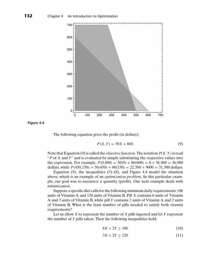
132 Chapter 4 An Introduction to Optimization
700
600
500
400
300
200
100
00 100 200 300 400 600500 700
Figure 4.4
The following equation gives the profit (in dollars):
P(X, Y ) = 50X + 60Y. (9)
Note that Equation (9) is called the objective function. The notation P(X, Y ) is read“P of X and Y” and is evaluated by simply substituting the respective values intothe expression. For example, P(0,600) = 50(0) + 60(600) = 0 + 36,000 = 36,000dollars, while P(450,150) = 50(450) + 60(150) = 22,500 + 9000 = 31,500 dollars.
Equation (9), the inequalities (5)–(8), and Figure 4.4 model the situationabove, which is an example of an optimization problem. In this particular exam-ple, our goal was to maximize a quantity (profit). Our next example deals withminimization.
Suppose a specific diet calls for the following minimum daily requirements: 186units of Vitamin A and 120 units of Vitamin B. Pill X contains 6 units of VitaminA and 3 units of Vitamin B, while pill Y contains 2 units of Vitamin A and 2 unitsof Vitamin B. What is the least number of pills needed to satisfy both vitaminrequirements?
Let us allow X to represent the number of X pills ingested and let Y representthe number of Y pills taken. Then the following inequalities hold:
6X + 2Y ≥ 186 (10)
3X + 2Y ≥ 120 (11)

4.2 Modeling with Inequalities 133
100
80
60
40
20
00 20 40 60 80 100
Figure 4.5
X ≥ 0 (12)
Y ≥ 0. (13)
Note that (10) models the minimum daily requirement of units ofVitaminA,while(11) refers to the minimum daily requirement of units of Vitamin B. The quantityto be minimized, the total number of pills, is given by the objective function:
N(X, Y) = X + Y. (14)
We note that while this region of feasibility is convex, it is also unbounded. Ourvertices are (40, 0), (0, 93), and (22, 27).
In the next section we will solve problems such as these by applying a verysimple, yet extremely powerful, theorem of linear programming.
Problems 4.2
Model the following situations by defining all variables and giving all inequalities,the objective function and the region of feasibility.
1. Farmer John gets $5000 for every truck of wheat sold and $6000 for every truckof corn sold. He has two fields: field A has 23 acres and field B has 17 acres.

134 Chapter 4 An Introduction to Optimization
For every 2 acres of field A, Farmer John produces a truck of wheat, while3 acres are required of field B for the same amount of wheat. Regarding thecorn, 3 acres of field A are required for a truck, while only 1 acre of field B isneeded. How many trucks of each commodity should be produced to maximizeFarmer John’s profit?
2. Redo Problem (1) if Farmer John gets $8000 for every truck of wheat and $5000for every truck of corn.
3. Dr. Lori Pesciotta, a research scientist, is experimenting with two forms of aspecial compound, H-Turebab. She needs at least 180 units of one form of thecompound (α) and at least 240 units of the second form of the compound (β).Two mixtures are used: X and Y . Every unit of X contains two units of α andthree units of β, while each unit of Y has the opposite concentration. Whatcombination of X and Y will minimize Dr. Pesciotta’s costs, if each unit of X
costs $500 and each unit of Y costs $750?
4. Redo Problem (3) if X costs $750 per unit and Y costs $500 per unit.
5. Redo Problem (3) if, in addition, Dr. Pesciotta needs at least 210 units of athird form (γ) of H-Turebab, and it is known that every unit of both X and Y
contains 10 units of γ .
6. Cereal X costs $.05 per ounce while Cereal Y costs $.04 per ounce. Everyounce of X contains 2 milligrams (mg) of Zinc and 1 mg of Calcium, whileevery ounce of Y contains 1 mg of Zinc and 4 mg of Calcium. The minimumdaily requirement (MDR) is 10 mg of Zinc and 15 mg of Calcium. Find theleast expensive combination of the cereals which would satisfy the MDR.
7. Redo Problem (6) with the added constraint of at least 12 mg of Sodium if eachounce of X contains 3 mg of Sodium and every ounce of Y has 2 mg of Sodium.
8. Redo Problem (7) if Cereal X costs $.07 an ounce and Cereal Y costs $.08 anounce.
9. Consider the following group of inequalities along with a corresponding objec-tive function. For each one, sketch the region of feasibility (except for 9 g) andconstruct a scenario that might model each set of inequalities:
(a) x ≥ 0, y ≥ 0, 2x + 5y ≤ 10, 3x + 4y ≤ 12, F(x, y) = 100x + 55y
(b) x ≥ 0, y ≤ 0, x + y ≤ 40, x + 2y ≤ 60, G(x, y) = 7x + 6y
(c) x ≥ 2, y ≥ 3, x + y ≤ 40, x + 2y ≤ 60, H(x, y) = x + 3y
(d) x ≥ 0, y ≥ 0, x + y ≤ 600, 3x + y ≤ 900, x + 2y ≤ 1000, J(x, y) = 10x + 4y
(e) 2x + 9y ≥ 1800, 3x + y ≥ 750, K(x, y) = 4x + 11y
(f ) x + y ≥ 100, x + 3y ≥ 270, 3x + y ≥ 240, L(x, y) = 600x + 375y
(g) x ≥ 0, y ≥ 0, z ≥ 0, x + y + 2z ≤ 12, 2x + y + z ≤ 14, x + 3y + z ≤ 15,
M(x, y, z) = 2x + 3y + 4z (Do not sketch the region of feasibility for thisproblem.)

4.3 Solving Problems Using Linear Programming 135
4.3 Solving Problems Using Linear Programming
We are now ready to solve a fairly large class of optimization problems usinga special form of the Fundamental Theorem of Linear Programming. We willnot prove this theorem, but many references to the proof of a more generalresult are available (for example, see Luenberger, D. G., Linear and NonlinearProgramming, 2nd Ed., Springer 2003).
The Fundamental Theorem of Linear Programming Let be a convex regionof feasibility in the xy-plane. Then the objective function F(x, y) = ax + by, wherea and b are real numbers, takes on both maximum and minimum values—if theyexist—on one or more vertices of .
Remark 1 The theorem holds only if maximum and/or minimum values exist.
Remark 2 It is possible to have infinitely many values where an optimal (max-imum or minimum) value exists. In this case, they would lie on one of the linesegments that form the boundary of the region of feasibility. See Example 3 below.
Remark 3 The word programming has nothing to do with computer program-ming, but rather the systematic order followed by the procedure, which can alsobe termed an algorithm.
Some examples are in order.
Example 1 (Wagons): Consider the inequalities (5) through (8), along withEquation (9), from Section 4.2. We again give the region of feasibility belowin Figure 4.6 (same as Figure 4.4):
Evaluation our objective function,
P(X, Y) = 50X + 60Y, (15)
at each of the four vertices yields the following results:
⎧⎪⎪⎨⎪⎪⎩
P(0,0) = 0P(0,600) = 36,000P(450,150) = 31,500P(500,0) = 25,000.
By the Fundamental Theorem of Linear Programming, we see that the maxi-mum profit of $36,000 occurs if no X wagons are produced and 600 Y wagons aremade. �

136 Chapter 4 An Introduction to Optimization
700
600
500
400
300
200
100
00 100 200 300 400 600500 700
Figure 4.6
Example 2 (Wagons): Suppose the profit function in the previous example isgiven by
R(X, Y) = 80X + 50Y. (16)
Then
⎧⎪⎪⎨⎪⎪⎩
R(0,0) = 0R(0,600) = 30,000R(450,150) = 43,500R(500,0) = 40,000.
We see, in this situation, that the maximum profit of $43,500 occurs if 450 X
wagons are produced, along with 150 Y wagons. �
Example 3 (Wagons): Consider the examples above with the profit functiongiven by
L(X, Y) = 75X + 75Y. (17)

4.3 Solving Problems Using Linear Programming 137
Then ⎧⎪⎪⎨⎪⎪⎩
L(0,0) = 0L(0,600) = 45,000L(450,150) = 45,000L(500,0) = 37,500.
Note that we have two situations in which the profit is maximized at $45,000; infact, there are many points where this occurs. For example,
L(300, 300) = 45,000. (18)
This occurs at any point along the constraint given by inequality (2). The reasonlies in the fact that coefficients of X and Y in (2) and in Equation (7) have the sameratio. �
Example 4 (Vitamins): Consider constraints (10) through (13) above inSection 4.2; minimize the objective function given by Equation (14).
N(X, Y) = X + Y. (19)
�
The region of feasibility (same as Figure 4.5) is given below in Figure 4.7:Evaluating our objective function (19) at the three vertices, we find that⎧⎨
⎩N(40, 0) = 40N(0, 93) = 93N(22, 27) = 49,
so the minimum number of pills needed to satisfy the minimum daily requirementis 40.
Sometimes a constraint is redundant; that is, the other constraints “include”the redundant constraint.
For example, suppose we want to maximize the objective function
Z(X, Y) = 4X + 3Y, (20)
given the constraints
4X + 2Y ≤ 40 (21)
3X + 4Y ≤ 60 (22)
X ≥ 0 (23)
Y ≥ 0. (24)

138 Chapter 4 An Introduction to Optimization
100
80
60
40
20
00 20 40 60 80 100
Figure 4.7
The vertices of the region of feasibility are (0, 0), (0, 15), (4, 12), and (10, 0), asseen below in Figure 4.8.
Note that (11) is maximized at Z(4, 12) = 52.Suppose we now add a third constraint:
X + Y ≤ 30. (25)
Figure 4.9 below reflects this added condition. Note, however, that the region offeasibility is not changed and the four vertices are unaffected by this redundantconstraint. It follows, therefore, that our objective function Z(X, Y) = 4X + 3Y isstill maximized at Z(4, 12) = 52.
Remark 4 Sometimes a vertex does not have whole number coordinates (seeproblem (15) below). If the physical model does not make sense to have a frac-tional or decimal answer—for example 2.5 bicycles or 1/3 cars—then we shouldcheck the closest points with whole number coordinates, provided these pointslie in the region of feasibility. For example, if (2.3, 7.8) is the vertex which givesthe optimal value for an objective function, then the following points should bechecked: (2, 7), (2, 8), (3, 7) and (3, 8).

4.3 Solving Problems Using Linear Programming 139
40
30
20
10
00 10 20 30 40
Figure 4.8
40
30
20
10
00 10 20 30 40
Figure 4.9

140 Chapter 4 An Introduction to Optimization
Problems 4.3
Using linear programming techniques, solve the following problems.
1. Section 4.2, Problem (1).
2. Section 4.2, Problem (2).
3. Section 4.2, Problem (3).
4. Section 4.2, Problem (4).
5. Section 4.2, Problem (5).
6. Section 4.2, Problem (6).
7. Section 4.2, Problem (7).
8. Section 4.2, Problem (8).
9. Section 4.2, Problem (9a); maximize F(x, y).
10. Section 4.2, Problem (9b); maximize G(x, y).
11. Section 4.2, Problem (9c); maximize H(x, y).
12. Section 4.2, Problem (9d); maximize J(x, y).
13. Section 4.2, Problem (9e); minimize K(x, y).
14. Section 4.2, Problem (9f); minimize L(x, y).
15. Maximize P(x, y) = 7x + 6y subject to the constraints x ≥ 0, y ≥ 0, 2x + 3y ≤1200 and 6x + y ≤ 1500.
4.4 An Introduction to the Simplex Method
In most of the problems considered in the previous section, we had but twovariables (usually X and Y) and two constraints, not counting the usual condi-tions of the non-negativity of X and Y . Once a third constraint is imposed, theregion of feasibility becomes more complicated; and, with a fourth constraint,even more so.
Also, if a third variable, say Z, is brought into the discussion, then theregion of feasibility becomes three-dimensional! This certainly makes the tech-nique employed in the previous section much more difficult to apply, althoughtheoretically it can be used.
We are fortunate that an alternate method exists which is valid for any numberof variables and any number of constraints. It is known as the Simplex Method.This is a classic method that has been in use for many years. The reader may wishto consult G. Hadley’s Linear Programming published by Addison-Wesley in 1963for the theoretical underpinnings of this algorithm.
Before we illustrate this technique with a number of examples, describing anddefining terms as we go along, we point out that this section will deal exclusively

4.4 An Introduction to the Simplex Method 141
with maximization problems. We will address minimization in the next, and final,section of this chapter.
Example 1 Suppose we want to maximize the following function of twovariables:
z = 7x1 + 22x2. (26)
Note that we are using xi instead of the usual x and y, due to the fact that, in laterexamples, we will have more than two independent variables.
Let us assume that the following constraints are imposed:
3x1 + 10x2 ≤ 33,000 (27)
5x1 + 8x2 ≤ 42,000 (28)
x1 ≥ 0 (29)
x2 ≥ 0. (30)
We now introduce the concept of slack variables, which we denote by si. Thesevariables (which can never be negative) will“pick up the slack”in the relationships(27) and (28) and convert these inequalities into equations. That is, (27) and (28)can now be written respectively as:
3x1 + 10x2 + s1 = 33,000 (31)
and
5x1 + 8x2 + s2 = 42,000. (32)
We also incorporate these slack variables into our objective function (26), rewritingit as:
−7x1 − 22x2 + 0s1 + 0s2 + z = 0. (33)
Finally, we rewrite (27) and (28) as
3x1 + 10x2 + s1 + 0s2 + 0z = 33,000 (34)
5x1 + 8x2 + 0s1 + 1s2 + 0z = 42,000. (35)
�
Remark 1 Admittedly, the Equations (33) through (35) seem somewhat strange.However, the reader will soon see why we have recast these equations as they nowappear.

142 Chapter 4 An Introduction to Optimization
We are now ready to put these last three equations into a table known as theinitial tableau. This is nothing more than a kind of augmented matrix. To do this,we merely “detach” the coefficients of the five unknowns (x1, x2, s1, s2, and z) andform the following table:
x1 x2 s1 s2 z⎡⎣ 3 10 1 0 0 33,000
5 8 0 1 0 42,000−7 −22 0 0 1 0
⎤⎦. (36)
Remark 2 Note that the objective function equation—here, Equation (33)—is in the bottom row. Also, unless otherwise stipulated, we shall always assumethat the decision variables—that is, x1 and x2—are non-negative. Notice, too, thevertical bar that appears to the left of the rightmost column and the horizontal barplaced above the bottom row. Finally, we point out that the entry in the last rowand last column is always zero for this initial tableau. These conventions will assistus in interpreting the end state of the Simplex Method.
Before continuing with the Simplex Method, let us consider another example.
Example 2 Put the following maximization problem into the initial tableauform: z = 4x1 + 7x2 + 9x3, where x1 + x2 + 6x3 ≤ 50, 2x1 + 3x2 ≤ 40, and 4x1 +9x2 + 3x3 ≤ 10.
Note that we have three independent (decision) variables (the xi) and that thethree constraints will give us three slack variables (the si). These lead us to thefollowing four equations:
−4x1 − 7x2 − 9x3 + 0s1 + 0s2 + 0s3 + z = 0 (37)
x1 + x2 + 6x3 + s1 + 0s2 + 0s3 + 0z = 50 (38)
2x1 + 0x2 + 3x3 + 0s1 + s2 + 0s3 + 0z = 40 (39)
4x1 + 9x2 + 3x3 + 0s1 + 0s2 + s3 + 0z = 10. (40)
The initial tableau for this example is given below:
x1 x2 x3 s1 s2 s3 z⎡⎢⎢⎣
1 1 6 1 0 0 0 502 0 3 0 1 0 0 404 9 3 0 0 1 0 10
−4 −7 −9 0 0 0 1 0
⎤⎥⎥⎦. (41)
�

4.4 An Introduction to the Simplex Method 143
We will now outline the steps in the Simplex Method:
● Change all inequalities into equations via the use of slack variables.
● Rewrite the objective function, z, in terms of slack variables, setting one sideof the equation equal to zero and keeping the coefficient of z equal to +1.
● The number of equations should equal the sum of the constraints plus one (theequation given by the objective function).
● Form the initial tableau, listing the constraints above the objective function,labeling the columns, beginning with the decision variables, followed by theslack variables, with z represented by the last column before the vertical bar.The last column should have all the “constants.”
● Locate the most negative number in the last row. If more than one equally neg-ative number is present, arbitrarily choose any one of them. Call this numberk. This column will be called the work column.
● Consider each positive element in the work column. Divide each of theseelements into the corresponding row entry element in the last column. Theratio that is the smallest will be used as the work column’s pivot. If there ismore than one smallest ratio, arbitrarily choose any one of them.
● Use elementary row operations (see Chapter 2) to change the pivot elementto 1, unless it is already 1.
● Use elementary row operations to transform all the other elements in the workcolumn to 0.
● A column is reduced when all the elements are 0, with the exception of thepivot, which is 1.
● Repeat the process until there are no negative elements in the last row.
● We are then able to determine the answers from this final tableau.
Let us illustrate this by returning to Example 1, where the initial tableau isgiven by
x1 x2 s1 s2 z⎡⎣ 3 10 1 0 0 33,000
5 8 0 1 0 42,000−7 −22 0 0 1 0
⎤⎦. (42)
We first note that −22 is the most negative number in the last row of (42). So the“x2” column is our work column.
We next divide 33,000 by 10 = 3300 and 42,000 by 8 = 5250; since 3300 is thelesser positive number, we will use 10 as the pivot. Note that we have put a carat

144 Chapter 4 An Introduction to Optimization
(∧) over the 10 to signify it is the pivot element.
x1 x2 s1 s2 z⎡⎣ 3 10 1 0 0 33,000
5 8 0 1 0 42,000−7 −22 0 0 1 0
⎤⎦. (43)
We now divide every element in the row containing the pivot by 10.
x1 x2 s1 s2 z⎡⎣ 0.3 1 0.1 0 0 3300
5 8 0 1 0 42,000−7 −22 0 0 1 0
⎤⎦. (44)
Next, we use elementary row operations; we multiply the first row by −8 and addit to the second row and multiply the first row by 22 and add it to the third row.This will give us a 0 for every element (other than the pivot) in the work column.
x1 x2 s1 s2 z⎡⎣ 0.3 1 0.1 0 0 3300
2.6 0 −0.8 1 0 15,600−0.4 0 2.2 0 1 72,600
⎤⎦. (45)
And now we repeat the process because we still have a negative entry in thelast row; that is, −0.4 is in the “x1” column. Hence, this becomes our new workcolumn.
Dividing 3300 by 0.3 yields 11,000; dividing 15,600 by 2.6 gives us 6000; since6000 is the lesser of the two positive ratios, we will use the 2.6 entry as the pivot(again denoting it with a carat, and removing the carat from our first pivot).
x1 x2 s1 s2 z⎡⎣ 0.3 1 0.1 0 0 3300
ˆ2.6 0 −0.8 1 0 15,600−0.4 0 2.2 0 1 72,600
⎤⎦. (46)
Dividing each element in this row by 2.6 gives us the following tableau:
x1 x2 s1 s2 z⎡⎣ 0.3 1 0.1 0 0 3300
1 0 −.31 .38 0 6000−0.4 0 2.2 0 1 72,600
⎤⎦. (47)
Using our pivot and elementary row operations, we transform every other elementin this work column to 0. That is, we multiply each element in the second row by

4.4 An Introduction to the Simplex Method 145
−0.3 and add the row to the first row and we multiply every element in the secondrow by 0.4 and add the row to the last row. This gives us the following tableau:
x1 x2 s1 s2 z⎡⎣ 0 1 0.19 −0.12 0 1500
1 0 −.31 .38 0 60000 0 2.08 0.15 1 75,000
⎤⎦. (48)
We are now finished with the process, because there are no negative elements inthe last row. We interpret this final tableau as follows:
● x1 = 6000 (note the “1” in the x1 column and the “0” in the x2 column).
● x2 = 1500 (note the “0” in the x1 column and the “1” in the x2 column).
● Both slack variables equal 0. To verify this, please see Equations (31) and (32)and substitute our values for x1 and x2 into these equations.
● The maximum value of z is 75,000 (found in the lower right-hand corner box).
We now give another example.
Example 3 Maximize z = x1 + 2x2, subject to the constraints 4x1 + 2x2 ≤ 40and 3x1 + 4x2 ≤ 60.
Following the practice discussed in this section and introducing the slackvariables, we have:
4x1 + 2x2 + s1 = 40 (49)
3x1 + 4x2 + s2 = 60 (50)
and
−x1 − 2x2 + z = 0. (51)
We form the initial tableau, using coefficients of 0 where needed, as follows:
x1 x2 s1 s2 z⎡⎣ 4 2 1 0 0 40
3 4 0 1 0 60−1 −2 0 0 1 0
⎤⎦. (52)
The second column will be our work column, since −2 is the most negative entry.Dividing 40 by 2 gives 20; dividing 60 by 4 yields 15. Since 15 is a lesser positive

146 Chapter 4 An Introduction to Optimization
ratio than 20, we will use the 4 as the pivot:
x1 x2 s1 s2 z⎡⎣ 4 2 1 0 0 40
3 4 0 1 0 60−1 −2 0 0 1 0
⎤⎦. (53)
Dividing every element of the second row will make our pivoting element 1:
x1 x2 s1 s2 z⎡⎣ 4 2 1 0 0 40
0.75 1 0 0.25 0 15−1 −2 0 0 1 0
⎤⎦. (54)
We now use our pivot, along with the proper elementary row operations, to makeevery other element in the column zero. This leads to the following tableau:
x1 x2 s1 s2 z⎡⎣ 2.5 0 1 −0.5 0 10
0.75 1 0 0.25 0 150.5 0 0 0.5 1 30
⎤⎦. (55)
Since the last row has no negative entries, we are finished and have the finaltableau:
x1 x2 s1 s2 z⎡⎣ 2.5 0 1 −0.5 0 10
0.75 1 0 0.25 0 150.5 0 0 0.5 1 30
⎤⎦. (56)
This final tableau is a little more complicated to interpret than (48).
First notice the “1” in the second row; this implies that x2 = 15. Thecorresponding equation represented by this second row thereby reduces to
0.75x1 + 15 + 0.25s2 = 15. (57)
Which forces both x1 and s2 to be zero, since neither can be negative. This forcess1 = 10, as we can infer from the equation represented by the first row:
0.25x1 + s1 − 0.5s2 = 10. (58)
In practice, we are not concerned with the values of the slack variables, so we sum-marize by simply saying that our answers are x1 = 0 and x2 = 15 with a maximumvalue of z = 30. �

4.5 Final Comments 147
As we have pointed out, this is a classic technique. However, as the numberof variables (decision and/or slack) increases, the calculations can be somewhatburdensome. Thankfully, there are many software packages to assist in this matter.Please refer to the Final Comments at the end of this chapter.
One final remark:As is the case with linear programming, if there are an infinitenumber of optimal solutions, the Simplex Method does not give all solutions.
Problems 4.4
Using the Simplex Method, solve the following problems:
1. Section 4.2, Problem (1).
2. Section 4.2, Problem (2).
3. Maximize z = 3x1 + 5x2, subject to x1 + x2 ≤ 6 and 2x1 + x2 ≤ 8.
4. Maximize z = 8x1 + x2, subject to the same constraints in (3).
5. Maximize z = x1 + 12x2, subject to the same constraints in (3).
6. Maximize z = 3x1 + 6x2, subject to the constraints x1 + 3x2 ≤ 30, 2x1 + 2x2 ≤40, and 3x1 + x2 ≤ 30.
7. Consider problem (9) at the end of Section 4.2. Set up the initial tableaus forproblems (9a) through (9d).
4.5 Final Comments on Chapter 4
In this chapter we covered two approaches to optimization, the Linear Program-ming Method and the Simplex Method. Both of these techniques are classicaland their geometrics and algebraic simplicity reflect both the beauty and powerof mathematics.
Our goal was to introduce the reader to the basics of these “simple” methods.However, he or she should be cautioned with regard to the underlying theory.That is, many times in mathematics we have elegant results (theorems) whichare proved using very deep and subtle mathematical concepts with respect to theproofs of these theorems.
As we mentioned in the last section, the calculations, while not difficult, canbe a burden. Calculators and software packages can be of great assistance here.
We close with two observations. Please note that we have considered veryspecial cases where the constraints of the “≤” variety had positive quantitieson the right-hand side. If this is not the case for all the constraints, then wemust use an enhanced version of the Simplex Method (see, for example, FiniteMathematics: A Modeling Approach by R. Bronson and G. Bronson publishedby West in 1996).

148 Chapter 4 An Introduction to Optimization
Similarly, regarding the solving of minimization problems via the SimplexMethod, we essentially consider the “negation” of the objective function, andthen apply a modified version of the Simplex Method. For example, suppose wewanted to minimize z = 3x1 + 2x2, subject to the same constraints. In this case wewould maximize Z = −z = −3x1 − 2x2 while recasting our constraints, and thenproceed with the Simplex Method.

55Determinants
5.1 Introduction
Every square matrix has associated with it a scalar called its determinant. To beextremely rigorous we would have to define this scalar in terms of permutationson positive integers. However, since in practice it is difficult to apply a definitionof this sort, other procedures have been developed which yield the determinant ina more straightforward manner. In this chapter, therefore, we concern ourselvessolely with those methods that can be applied easily. We note here for referencethat determinants are only defined for square matrices.
Given a square matrix A, we use det(A) or |A| to designate its determinant. Ifthe matrix can actually be exhibited, we then designate the determinant of A byreplacing the brackets by vertical straight lines. For example, if
A =⎡⎣1 2 3
4 5 67 8 9
⎤⎦ (1)
then
det(A) =∣∣∣∣∣∣1 2 34 5 67 8 9
∣∣∣∣∣∣. (2)
We cannot overemphasize the fact that (1) and (2) represent entirely differentanimals. (1) represents a matrix, a rectangular array, an entity unto itself while (2)represents a scalar, a number associated with the matrix in (1). There is absolutelyno similarity between the two other than form!
We are now ready to calculate determinants.
Definition 1 The determinant of a 1 × 1 matrix [a] is the scalar a.
Thus, the determinant of the matrix [5] is 5 and the determinant of the matrix[−3] is −3.
149

150 Chapter 5 Determinants
Definition 2 The determinant of a 2 × 2 matrix
[a b
c d
]
is the scalar ad − bc.
Example 1 Find det(A) if
A =[
1 24 3
].
Solution
det(A) =∣∣∣∣1 24 3
∣∣∣∣ = (1)(3) − (2)(4) = 3 − 8 = −5. �
Example 2 Find |A| if
A =[
2 −14 3
].
Solution
|A| =∣∣∣∣2 −14 3
∣∣∣∣ = (2)(3) − (−1)(4) = 6 + 4 = 10. �
We now could proceed to give separate rules which would enable one to com-pute determinants of 3 × 3, 4 × 4, and higher order matrices. This is unnecessary.In the next section, we will give a method that enables us to reduce all determi-nants of order n(n > 2) (if A has order n × n then det(A) is said to have order n)to a sum of determinants of order 2.
Problems 5.1
In Problems 1 through 18, find the determinants of the given matrices.
1.[
3 45 6
], 2.
[3 −45 6
], 3.
[3 4
−5 6
],
4.[
5 67 8
], 5.
[5 6
−7 8
], 6.
[5 67 −8
],

5.1 Introduction 151
7.[
1 −12 7
], 8.
[−2 −3−4 4
], 9.
[3 −1
−3 8
],
10.[
0 1−2 6
], 11.
[−2 3−4 −4
], 12.
[9 02 0
],
13.[
12 20−3 −5
], 14.
[−36 −3−12 −1
], 15.
[−8 −3−7 9
],
16.[t 23 4
], 17.
[2t 3
−2 t
], 18.
[3t −t2
2 t
].
19. Find t so that ∣∣∣∣ t 2t
1 t
∣∣∣∣ = 0.
20. Find t so that ∣∣∣∣t − 2 t
3 t + 2
∣∣∣∣ = 0.
21. Find λ so that ∣∣∣∣4 − λ 2−1 1 − λ
∣∣∣∣ = 0.
22. Find λ so that ∣∣∣∣1 − λ 51 −1 − λ
∣∣∣∣ = 0.
23. Find det(A − λI) if A is the matrix defined in Problem 1.
24. Find det(A − λI) if A is the matrix defined in Problem 2.
25. Find det(A − λI) if A is the matrix defined in Problem 4.
26. Find det(A − λI) if A is the matrix defined in Problem 7.
27. Find |A|, |B|, and |AB| if
A =[
1 32 1
]and B =
[4 2
−1 2
].
What is the relationship between these three determinants?
28. Interchange the rows for each of the matrices given in Problems 1 through15, and calculate the new determinants. How do they compare with thedeterminants of the original matrices?

152 Chapter 5 Determinants
29. The second elementary row operation is to multiply any row of a matrixby a nonzero constant. Apply this operation to the matrices given in Prob-lems 1 through 15 for any constants of your choice, and calculate the newdeterminants. How do they compare with the determinants of the originalmatrix?
30. Redo Problem 29 for the third elementary row operation.
31. What is the determinant of a 2 × 2 matrix if one row or one column containsonly zero entries?
32. What is the relationship between the determinant of a 2 × 2 matrix and itstranspose?
33. What is the determinant of a 2 × 2 matrix if one row is a linear combinationof the other row?
5.2 Expansion by Cofactors
Definition 1 Given a matrix A, a minor is the determinant of any squaresubmatrix of A.
That is, given a square matrix A, a minor is the determinant of any matrixformed from A by the removal of an equal number of rows and columns. As anexample, if
A =⎡⎣1 2 3
4 5 67 8 9
⎤⎦,
then ∣∣∣∣1 27 8
∣∣∣∣ and∣∣∣∣5 68 9
∣∣∣∣are both minors because [
1 27 8
]and
[5 68 9
]
are both submatrices of A, while[1 28 9
]and
∣∣1 2∣∣
are not minors because [1 28 9
]
is not a submatrix of A and [1 2], although a submatrix of A, is not square.

5.2 Expansion by Cofactors 153
A more useful concept for our immediate purposes, since it will enable us tocalculate determinants, is that of the cofactor of an element of a matrix.
Definition 2 Given a matrix A =[aij
], the cofactor of the element aij is a
scalar obtained by multiplying together the term (−1)i + j and the minor obtainedfrom A by removing the ith row and jth column.
In other words, to compute the cofactor of the element aij we first form asubmatrix of A by crossing out both the row and column in which the element aij
appears. We then find the determinant of the submatrix and finally multiply it bythe number (−1)i + j .
Example 1 Find the cofactor of the element 4 in the matrix
A =⎡⎣1 2 3
4 5 67 8 9
⎤⎦.
Solution We first note that 4 appears in the (2, 1) position. The submatrixobtained by crossing out the second row and first column is⎡
⎣1 2 34 5 67 8 9
⎤⎦ =
[2 38 9
],
which has a determinant equal to (2)(9) − (3)(8) = −6. Since 4 appears in the (2, 1)position, i = 2 and j = 1. Thus, (−1)i+j = (−1)2+1 = (−1)3 = (−1). The cofactorof 4 is (−1)(−6) = 6. �
Example 2 Using the sameA as in Example 1, find the cofactor of the element 9.
Solution The element 9 appears in the (3, 3) position. Thus, crossing out thethird row and third column, we obtain the submatrix⎡
⎣1 2 34 5 67 8 9
⎤⎦ =
[1 24 5
].
which has a determinant equal to (1)(5) − (2)(4) = −3. Since, in this case, i = j =3, the cofactor of 9 is (−1)3 + 3(−3) = (−1)6(−3) = −3. �
We now have enough tools at hand to find the determinant of any matrix.
Expansion by Cofactors. To find the determinant of a matrix A of arbitrary order,(a) pick any one row or any one column of the matrix (dealer’s choice), (b) for

154 Chapter 5 Determinants
each element in the row or column chosen, find its cofactor, (c) multiply eachelement in the row or column chosen by its cofactor and sum the results. This sumis the determinant of the matrix.
Example 3 Find det(A) if
A =⎡⎣ 3 5 0
−1 2 13 −6 4
⎤⎦.
Solution In this example, we expand by the second column.
|A| = (5)(cofactor of 5) + (2)(cofactor of 2) + (−6)(cofactor of −6)
= (5)(−1)1 + 2∣∣∣∣−1 1
3 4
∣∣∣∣+ (2)(−1)2 + 2∣∣∣∣3 03 4
∣∣∣∣+ (−6)(−1)3 + 2∣∣∣∣ 3 0−1 1
∣∣∣∣= 5(−1)(−4 − 3) + (2)(1)(12 − 0) + (−6)(−1)(3 − 0)
= (−5)(−7) + (2)(12) + (6)(3) = 35 + 24 + 18 = 77. �
Example 4 Using the A of Example 3 and expanding by the first row, finddet(A).
Solution
|A| = 3(cofactor of 3) + 5(cofactor of 5) + 0(cofactor of 0)
= (3)(−1)1 + 1∣∣∣∣ 2 1−6 4
∣∣∣∣+ 5(−1)1 + 2∣∣∣∣−1 1
3 4
∣∣∣∣+ 0
= (3)(1)(8 + 6) + (5)(−1)(−4 − 3)
= (3)(14) + (−5)(−7) = 42 + 35 = 77. �
The previous examples illustrate two important properties of the method. First,the value of the determinant is the same regardless of which row or column wechoose to expand by and second, expanding by a row or column that containszeros significantly reduces the number of computations involved.
Example 5 Find det(A) if
A =
⎡⎢⎢⎣
1 0 5 2−1 4 1 0
3 0 4 1−2 1 1 3
⎤⎥⎥⎦.

5.2 Expansion by Cofactors 155
Solution We first check to see which row or column contains the most zeros andexpand by it. Thus, expanding by the second column gives
|A| = 0(cofactor of 0) + 4(cofactor of 4) + 0(cofactor of 0) + 1(cofactor of 1)
= 0 + 4(−1)2+2
∣∣∣∣∣∣1 5 23 4 1
−2 1 3
∣∣∣∣∣∣+ 0 + 1(−1)4+2
∣∣∣∣∣∣1 5 2
−1 1 03 4 1
∣∣∣∣∣∣= 4
∣∣∣∣∣∣1 5 23 4 1
−2 1 3
∣∣∣∣∣∣+∣∣∣∣∣∣
1 5 2−1 1 0
3 4 1
∣∣∣∣∣∣.Using expansion by cofactors on each of the determinants of order 3 yields
∣∣∣∣∣∣1 5 23 4 1
−2 1 3
∣∣∣∣∣∣ = 1(−1)1+1∣∣∣∣4 11 3
∣∣∣∣+ 5(−1)1+2∣∣∣∣ 3 1−2 3
∣∣∣∣+ 2(−1)1+3∣∣∣∣ 3 4−2 1
∣∣∣∣= −22 (expanding by the first row)
and ∣∣∣∣∣∣1 5 2
−1 1 03 4 1
∣∣∣∣∣∣ = 2(−1)1+3∣∣∣∣−1 1
3 4
∣∣∣∣+ 0 + 1(−1)3+3∣∣∣∣ 1 5−1 1
∣∣∣∣= −8 (expanding by the third column).
Hence,
|A| = 4(−22) − 8 = −88 − 8 = −96. �
For n × n matrices with n > 3, expansion by cofactors is an inefficient pro-cedure for calculating determinants. It simply takes too long. A more elegantmethod, based on elementary row operations, is given in Section 5.4 for matriceswhose elements are all numbers.
Problems 5.2
In Problems 1 through 22, use expansion by cofactors to evaluate the determinantsof the given matrices.
1.
⎡⎣1 2 −2
0 2 30 0 −3
⎤⎦, 2.
⎡⎣3 2 −2
1 0 42 0 −3
⎤⎦, 3.
⎡⎣1 −2 −2
7 3 −30 0 0
⎤⎦,

156 Chapter 5 Determinants
4.
⎡⎣2 0 −1
1 1 13 2 −3
⎤⎦, 5.
⎡⎣ 3 5 2
−1 0 4−2 2 7
⎤⎦, 6.
⎡⎣1 −3 −3
2 8 34 5 0
⎤⎦,
7.
⎡⎣2 1 −9
3 −1 13 −1 2
⎤⎦, 8.
⎡⎣−1 3 3
1 1 4−1 1 2
⎤⎦, 9.
⎡⎣1 −3 −3
2 8 43 5 1
⎤⎦,
10.
⎡⎣2 1 3
3 −1 22 3 5
⎤⎦, 11.
⎡⎣−1 3 3
4 5 6−1 3 3
⎤⎦, 12.
⎡⎣1 2 −3
5 5 12 −5 −1
⎤⎦,
13.
⎡⎣−4 0 0
2 −1 03 1 −2
⎤⎦, 14.
⎡⎣ 1 3 2
−1 4 15 3 8
⎤⎦, 15.
⎡⎣ 3 −2 0
1 1 2−3 4 1
⎤⎦,
16.
⎡⎢⎢⎣
−4 0 0 01 −5 0 02 1 −2 03 1 −2 1
⎤⎥⎥⎦, 17.
⎡⎢⎢⎣
−1 2 1 21 0 3 −12 2 −1 12 0 −3 2
⎤⎥⎥⎦,
18.
⎡⎢⎢⎣
1 1 2 −21 5 2 −1
−2 −2 1 3−3 4 −1 8
⎤⎥⎥⎦, 19.
⎡⎢⎢⎣
−1 3 2 −21 −5 −4 63 −6 1 13 −4 3 −3
⎤⎥⎥⎦,
20.
⎡⎢⎢⎣
1 1 0 −21 5 0 −1
−2 −2 0 3−3 4 0 8
⎤⎥⎥⎦, 21.
⎡⎢⎢⎣
1 2 1 −14 0 3 01 1 0 52 −2 1 1
⎤⎥⎥⎦,
22.
⎡⎢⎢⎢⎢⎣
11 1 0 9 02 1 1 0 04 −1 1 0 03 2 2 1 00 0 1 2 0
⎤⎥⎥⎥⎥⎦.
23. Use the results of Problems 1, 13, and 16 to develop a theorem about thedeterminants of triangular matrices.
24. Use the results of Problems 3, 20, and 22 to develop a theorem regardingdeterminants of matrices containing a zero row or column.
25. Find det(A − λI) if A is the matrix given in Problem 2.
26. Find det(A − λI) if A is the matrix given in Problem 3.
27. Find det(A − λI) if A is the matrix given in Problem 4.
28. Find det(A − λI) if A is the matrix given in Problem 5.

5.3 Properties of Determinants 157
5.3 Properties of Determinants
In this section, we list some useful properties of determinants. For the sake ofexpediency, we only give proofs for determinants of order three, keeping in mindthat these proofs may be extended in a straightforward manner to determinantsof higher order.
Property 1 If one row of a matrix consists entirely of zeros, then the determinantis zero.
Proof. Expanding by the zero row, we immediately obtain the desired result.
Property 2 If two rows of a matrix are interchanged, the determinant changessign.
Proof. Consider
A =⎡⎣a11 a12 a13
a21 a22 a23a31 a32 a33
⎤⎦.
Expanding by the third row, we obtain
|A| = a31(a12 a23 − a13 a22) − a32(a11 a23 − a13 a21)
+ a33(a11 a22 − a12 a21).
Now consider the matrix B obtained from A by interchanging the second and thirdrows:
B =⎡⎣a11 a12 a13
a31 a32 a33a21 a22 a23
⎤⎦.
Expanding by the second row, we find that
|B| = −a31(a12 a23 − a13 a22) + a32(a11 a23 − a13 a21)
− a33(a11 a22 − a12 a21).
Thus, |B| = −|A|. Through similar reasoning, one can demonstrate that the resultis valid regardless of which two rows are interchanged.
Property 3 If two rows of a determinant are identical, the determinant is zero.

158 Chapter 5 Determinants
Proof. If we interchange the two identical rows of the matrix, the matrix remainsunaltered; hence the determinant of the matrix remains constant. From Property2, however, by interchanging two rows of a matrix, we change the sign of thedeterminant. Thus, the determinant must on one hand remain the same while onthe other hand change the sign. The only way both of these conditions can be metsimultaneously is for the determinant to be zero.
Property 4 If the matrix B is obtained from the matrix A by multiplying everyelement in one row of A by the scalar λ, then |B| = λ|A|.
Proof.
∣∣∣∣∣∣λa11 λa12 λa13a21 a22 a23a31 a32 a33
∣∣∣∣∣∣ = λa11
∣∣∣∣a22 a23a32 a33
∣∣∣∣− λa12
∣∣∣∣a21 a23a31 a33
∣∣∣∣+ λa13
∣∣∣∣a12 a22a31 a32
∣∣∣∣= λ
(a11
∣∣∣∣a22 a23a32 a33
∣∣∣∣− a12
∣∣∣∣a21 a23a31 a33
∣∣∣∣+ a13
∣∣∣∣a21 a22a31 a32
∣∣∣∣)
= λ
∣∣∣∣∣∣a11 a12 a13a21 a22 a23a31 a32 a33
∣∣∣∣∣∣.In essence, Property 4 shows us how to multiply a scalar times a determinant.
We know from Chapter 1 that multiplying a scalar times a matrix simply multipliesevery element of the matrix by that scalar. Property 4, however, implies that mul-tiplying a scalar times a determinant simply multiplies one row of the determinantby the scalar. Thus, while in matrices
8[
1 23 4
]=[
8 1624 32
],
in determinants we have
8∣∣∣∣1 23 4
∣∣∣∣ =∣∣∣∣ 1 224 32
∣∣∣∣,or alternatively
8∣∣∣∣1 23 4
∣∣∣∣ = 4(2)
∣∣∣∣1 23 4
∣∣∣∣ = 4∣∣∣∣2 43 4
∣∣∣∣ =∣∣∣∣ 2 412 16
∣∣∣∣.Property 5 For an n × n matrix A and any scalar λ, det(λA) = λn det(A).

5.3 Properties of Determinants 159
Proof. This proof makes continued use of Property 4.
det(λA) = det
⎧⎨⎩λ
⎡⎣a11 a12 a13
a21 a22 a23a31 a32 a33
⎤⎦⎫⎬⎭ = det
⎧⎨⎩⎡⎣λa11 λa12 λa13
λa21 λa22 λa23λa31 λa32 λa33
⎤⎦⎫⎬⎭
=∣∣∣∣∣∣λa11 λa12 λa13λa21 λa22 λa23λa31 λa32 λa33
∣∣∣∣∣∣ = λ
∣∣∣∣∣∣a11 a12 a13
λa21 λa22 λa23λa31 λa32 λa33
∣∣∣∣∣∣= (λ)(λ)
∣∣∣∣∣∣a11 a12 a13a21 a22 a23
λa31 λa32 λa33
∣∣∣∣∣∣ = λ(λ)(λ)
∣∣∣∣∣∣a11 a12 a13a21 a22 a23a31 a32 a33
∣∣∣∣∣∣= λ3 det(A).
Note that for a 3 × 3 matrix, n = 3.
Property 6 If a matrix B is obtained from a matrix A by adding to one row ofA, a scalar times another row of A, then |A| = |B|.
Proof. Let
A =⎡⎣a11 a12 a13
a21 a22 a23a31 a32 a33
⎤⎦
and
B =⎡⎣a11 a12 a13
a21 a22 a23a31 + λa11 a32 + λa12 a33 + λa13
⎤⎦,
where B has been obtained from A by adding λ times the first row of A to thethird row of A. Expanding |B| by its third row, we obtain
|B| = (a31 + λa11)
∣∣∣∣a12 a13a22 a23
∣∣∣∣− (a32 + λa12)
∣∣∣∣a11 a13a21 a23
∣∣∣∣+ (a33 + λa13)
∣∣∣∣a11 a12a21 a22
∣∣∣∣= a31
∣∣∣∣a12 a13a22 a23
∣∣∣∣− a32
∣∣∣∣a11 a13a21 a23
∣∣∣∣+ a33
∣∣∣∣a11 a12a21 a22
∣∣∣∣+ λ
{a11
∣∣∣∣a12 a13a22 a23
∣∣∣∣− a12
∣∣∣∣a11 a13a21 a23
∣∣∣∣+ a13
∣∣∣∣a11 a12a21 a22
∣∣∣∣}.

160 Chapter 5 Determinants
The first three terms of this sum are exactly |A| (expand |A| by its third row), whilethe last three terms of the sum are
λ
∣∣∣∣∣∣a11 a12 a13a21 a22 a23a11 a12 a13
∣∣∣∣∣∣(expand this determinant by its third row). Thus, it follows that
|B| = |A| + λ
∣∣∣∣∣∣a11 a12 a13a21 a22 a23a11 a12 a13
∣∣∣∣∣∣.From Property 3, however, this second determinant is zero since its first and thirdrows are identical, hence |B| = |A|.
The same type of argument will quickly show that this result is valid regardlessof the two rows chosen.
Example 1 Without expanding, show that
∣∣∣∣∣∣a b c
r s t
x y z
∣∣∣∣∣∣ =∣∣∣∣∣∣a − r b − s c − t
r + 2x s + 2y t + 2z
x y z
∣∣∣∣∣∣.Solution Using Property 6, we have that
∣∣∣∣∣∣a b c
r s t
x y z
∣∣∣∣∣∣ =∣∣∣∣∣∣a − r b − s c − t
r s t
x y z
∣∣∣∣∣∣,⎧⎨⎩
by adding to the firstrow (−1 ) times thesecond row
=∣∣∣∣∣∣a − r b − s c − t
r + 2x s + 2y t + 2z
x y z
∣∣∣∣∣∣.⎧⎨⎩
by adding to thesecond row ( 2) times thethird row
�
Property 7 det(A) = det(AT).
Proof. If
A =⎡⎣a11 a12 a13
a21 a22 a23a31 a32 a33
⎤⎦, then AT =
⎡⎣a11 a21 a31
a12 a22 a32a13 a23 a33
⎤⎦.

5.3 Properties of Determinants 161
Expanding det(AT) by the first column, it follows that
∣∣∣AT∣∣∣ = a11
∣∣∣∣a22 a32a23 a33
∣∣∣∣− a12
∣∣∣∣a21 a31a23 a33
∣∣∣∣+ a13
∣∣∣∣a21 a31a22 a32
∣∣∣∣= a11(a22 a33 − a32 a23) − a12(a21a33 − a31 a23) + a13(a21 a32 − a31 a22).
This, however, is exactly the expression we would obtain if we expand det(A) bythe first row. Thus
∣∣AT∣∣ = |A|.
It follows from Property 7 that any property about determinants dealing withrow operations is equally true for column operations (the analogous elementaryrow operation applied to columns), because a row operation on AT is the sameas a column operation on A. Thus, if one column of a matrix consists entirely ofzeros, then its determinant is zero; if two columns of a matrix are interchanged, thedeterminant changes the sign; if two columns of a matrix are identical, its determi-nant is zero; multiplying a determinant by a scalar is equivalent to multiplying onecolumn of the matrix by that scalar and then calculating the new determinant; andthe third elementary column operation when applied to a matrix does not changeits determinant.
Property 8 The determinant of a triangular matrix, either upper or lower, is theproduct of the elements on the main diagonal.
Proof. See Problem 2.
Property 9 If A and B are of the same order, then det(A) det(B) = det(AB).
Because of its difficulty, the proof of Property 9 is omitted here.
Example 2 Show that Property 9 is valid for
A =[
2 31 4
]and B =
[6 −17 4
].
Solution |A| = 5, |B| = 31.
AB =[
33 1034 15
]thus |AB| = 155 = |A||B|. �
Problems 5.3
1. Prove that the determinant of a diagonal matrix is the product of the elementson the main diagonal.

162 Chapter 5 Determinants
2. Prove that the determinant of an upper or lower triangular matrix is theproduct of the elements on the main diagonal.
3. Without expanding, show that∣∣∣∣∣∣a + x r − x x
b + y s − y y
c + z t − z z
∣∣∣∣∣∣ =∣∣∣∣∣∣a r x
b s y
c t z
∣∣∣∣∣∣.4. Verify Property 5 for λ = −3 and
A =⎡⎣2 1 0
5 −1 32 1 1
⎤⎦.
5. Verify Property 9 for
A =∣∣∣∣6 11 2
∣∣∣∣ and B =∣∣∣∣3 −12 1
∣∣∣∣.6. Without expanding, show that∣∣∣∣∣∣
2a 3r x
4b 6s 2y
−2c −3t −z
∣∣∣∣∣∣ = −12
∣∣∣∣∣∣a r x
b s y
c t z
∣∣∣∣∣∣.7. Without expanding, show that∣∣∣∣∣∣
a − 3b r − 3s x − 3y
b − 2c s − 2t y − 2z
5c 5t 5z
∣∣∣∣∣∣ = 5
∣∣∣∣∣∣a r x
b s y
c t z
∣∣∣∣∣∣.8. Without expanding, show that∣∣∣∣∣∣
a b c
r s t
x y z
∣∣∣∣∣∣ = −∣∣∣∣∣∣a x r
b y s
c z t
∣∣∣∣∣∣.9. Without expanding, show that∣∣∣∣∣∣
a b c
r s t
x y z
∣∣∣∣∣∣ = −14
∣∣∣∣∣∣2a 4b 2c
−r −2s −t
x 2y z
∣∣∣∣∣∣.10. Without expanding, show that∣∣∣∣∣∣
a − 3x b − 3y c − 3z
a + 5x b + 5y c + 5z
x y z
∣∣∣∣∣∣ = 0.
5.4 Pivotal Condensation 163
11. Without expanding, show that∣∣∣∣∣∣2a 3a c
2r 3r t
2x 3x z
∣∣∣∣∣∣ = 0.
12. Prove that if one column of a square matrix is a linear combination of anothercolumn, then the determinant of that matrix is zero.
13. Prove that if A is invertible, then det(A−1) = 1/ det(A).
5.4 Pivotal Condensation
Properties 2, 4, and 6 of the previous section describe the effects on the determi-nant of a matrix of applying elementary row operations to the matrix itself. Theycomprise part of an efficient algorithm for calculating determinants of matriceswhose elements are numbers. The technique is known as pivotal condensation: Agiven matrix is transformed into row-reduced form using elementary row opera-tions. A record is kept of the changes to the determinant as a result of Properties 2,4, and 6. Once the transformation is complete, the row-reduced matrix is in uppertriangular form, and its determinant is found easily by Property 8. In fact, sincea row-reduced matrix has either unity elements or zeros on its main diagonal, itsdeterminant will be unity if all its diagonal elements are unity, or zero if any onediagonal element is zero.
Example 1 Use pivotal condensation to evaluate∣∣∣∣∣∣1 2 3
−2 3 23 −1 1
∣∣∣∣∣∣.Solution ∣∣∣∣∣∣
1 2 3−2 3 2
3 −1 1
∣∣∣∣∣∣ =∣∣∣∣∣∣1 2 30 7 83 −1 1
∣∣∣∣∣∣⎧⎨⎩
Property 6: adding tothe second row (2)times the first row
=∣∣∣∣∣∣1 2 30 7 80 −7 −8
∣∣∣∣∣∣⎧⎨⎩
Property 6: adding tothe third row (−3)times the first row
= 7
∣∣∣∣∣∣1 2 30 1 8
70 −7 −8
∣∣∣∣∣∣{
Property 4: appliedto the second row

164 Chapter 5 Determinants
= 7
∣∣∣∣∣∣1 2 30 1 8
70 0 0
∣∣∣∣∣∣⎧⎨⎩
Property 6: addingto the third row (7)times the second row
= 7(0) = 0.{
Property 8 �
Example 2 Use pivotal condensation to evaluate
∣∣∣∣∣∣0 −1 41 −5 1
−6 2 −3
∣∣∣∣∣∣.Solution∣∣∣∣∣∣
0 −1 41 −5 1
−6 2 −3
∣∣∣∣∣∣ = (−1)
∣∣∣∣∣∣1 −5 10 −1 4
−6 2 −3
∣∣∣∣∣∣{
Property 2: interchangingthe first and second rows
= (−1)
∣∣∣∣∣∣1 −5 10 1 40 −28 3
∣∣∣∣∣∣⎧⎨⎩
Property 6: addingto the third row (6)times the first row
= (−1)(−1)
∣∣∣∣∣∣1 −5 10 1 −40 −28 3
∣∣∣∣∣∣{
Property 4: appliedto the second row
=∣∣∣∣∣∣1 −5 10 1 −40 0 −109
∣∣∣∣∣∣⎧⎨⎩
Property 6: addingto the third row (28)times the second row
= (−109)
∣∣∣∣∣∣1 −5 10 1 −40 0 1
∣∣∣∣∣∣{
Property 4: appliedto the third row
= (−109)(1) = −109.{Property 8 �
Pivotal condensation is easily coded for implementation on a computer.Although shortcuts can be had by creative individuals evaluating determinantsby hand, this rarely happens. The orders of most matrices that occur in practiceare too large and, therefore, too time consuming to consider hand calculations inthe evaluation of their determinants. In fact, such determinants can bring com-puter algorithms to their knees. As a result, calculating determinants is avoidedwhenever possible.
Still, when determinants are evaluated by hand, appropriate shortcuts aretaken, as illustrated in the next two examples. The general approach involvesoperating on a matrix so that one row or one column is transformed into a new

5.4 Pivotal Condensation 165
row or column containing at most one nonzero element. Expansion by cofactorsis then applied to that row or column.
Example 3 Evaluate ∣∣∣∣∣∣10 −6 −9
6 −5 −7−10 9 12
∣∣∣∣∣∣.Solution∣∣∣∣∣∣
10 −6 −96 −5 −7
−10 9 12
∣∣∣∣∣∣ =∣∣∣∣∣∣10 −6 −9
6 −5 −70 3 3
∣∣∣∣∣∣⎧⎨⎩
by adding (1) times thefirst row to the third row(Property 6)
=∣∣∣∣∣∣10 −6 −3
6 −5 −20 3 0
∣∣∣∣∣∣⎧⎨⎩
by adding (−1) times thesecond column to thethird column (Property 6)
= −3∣∣∣∣10 −3
6 −2
∣∣∣∣ {by expansion by cofactors
= −3(−20 + 18) = 6. �
Example 4 Evaluate ∣∣∣∣∣∣∣∣3 −1 0 20 1 4 13 −2 3 59 7 0 2
∣∣∣∣∣∣∣∣.Solution Since the third column already contains two zeros, it would seemadvisable to work on that one.∣∣∣∣∣∣∣∣
3 −1 0 20 1 4 13 −2 3 59 7 0 2
∣∣∣∣∣∣∣∣ =
∣∣∣∣∣∣∣∣3 −1 0 20 1 4 13 − 11
4 0 174
9 7 0 2
∣∣∣∣∣∣∣∣⎧⎪⎨⎪⎩
by adding(− 3
4
)times
the second row tothe third row.
= −4
∣∣∣∣∣∣∣3 −1 23 − 11
4174
9 7 2
∣∣∣∣∣∣∣{
by expansionby cofactors
= −4(
14
)∣∣∣∣∣∣3 −1 2
12 −11 179 7 2
∣∣∣∣∣∣{by Property 4

166 Chapter 5 Determinants
= (−1)
∣∣∣∣∣∣3 −1 20 −7 99 7 2
∣∣∣∣∣∣⎧⎨⎩
by adding (−4) timesthe first row to thesecond row
= (−1)
∣∣∣∣∣∣3 −1 20 −7 90 10 −4
∣∣∣∣∣∣⎧⎨⎩
by adding (−3) timesthe first row to thethird row
= (−1)(3)
∣∣∣∣−7 910 −4
∣∣∣∣{
by expansion bycofactors
= (−3)(28 − 90) = 186. �
Problems 5.4
In Problems 1 through 18, evaluate the determinants of the given matrices.
1.
⎡⎣1 2 −2
1 3 32 5 0
⎤⎦, 2.
⎡⎣1 2 3
4 5 67 8 9
⎤⎦, 3.
⎡⎣ 3 −4 2
−1 5 71 9 −6
⎤⎦,
4.
⎡⎣−1 3 3
1 1 4−1 1 2
⎤⎦, 5.
⎡⎣1 −3 −3
2 8 43 5 1
⎤⎦, 6.
⎡⎣2 1 −9
3 −1 13 −1 2
⎤⎦,
7.
⎡⎣2 1 3
3 −1 22 3 5
⎤⎦, 8.
⎡⎣−1 3 3
4 5 6−1 3 3
⎤⎦, 9.
⎡⎣1 2 −3
5 5 12 −5 −1
⎤⎦,
10.
⎡⎣2 0 −1
1 1 13 2 −3
⎤⎦, 11.
⎡⎣ 3 5 2
−1 0 4−2 2 7
⎤⎦, 12.
⎡⎣1 −3 −3
2 8 34 5 0
⎤⎦,
13.
⎡⎢⎢⎣
3 5 4 6−2 1 0 7−5 4 7 2
8 −3 1 1
⎤⎥⎥⎦, 14.
⎡⎢⎢⎣
−1 2 1 21 0 3 −12 2 −1 12 0 −3 2
⎤⎥⎥⎦,
15.
⎡⎢⎢⎣
1 1 2 −21 5 2 −1
−2 −2 1 3−3 4 −1 8
⎤⎥⎥⎦, 16.
⎡⎢⎢⎣
−1 3 2 −21 −5 −4 63 −6 1 13 −4 3 −3
⎤⎥⎥⎦,
17.
⎡⎢⎢⎣
1 1 0 −21 5 0 −1
−2 −2 0 3−3 4 0 8
⎤⎥⎥⎦, 18.
⎡⎢⎢⎣
−2 0 1 34 0 2 −2
−3 1 0 15 4 1 7
⎤⎥⎥⎦.

5.5 Inversion 167
19. What can you say about the determinant of an n × n matrix that has rank lessthan n?
20. What can you say about the determinant of a singular matrix?
5.5 Inversion
As an immediate consequence of Theorem 1 of Section 3.2 and the method ofpivotal condensation, we have:
Theorem 1 A square matrix has an inverse if and only if its determinant is notzero.
In this section, we develop a method to calculate inverses of nonsingular matri-ces using determinants. For matrices with order greater than 3 × 3, this method isless efficient than the one described in Section 3.2, and is generally avoided.
Definition 1 The cofactor matrix associated with an n × n matrix A is an n × n
matrix Ac obtained from A by replacing each element of A by its cofactor.
Example 1 Find Ac if
A =⎡⎣ 3 1 2
−2 5 41 3 6
⎤⎦.
Solution
Ac =
⎡⎢⎢⎢⎢⎢⎢⎢⎢⎣
(−1)1+1∣∣∣∣5 43 6
∣∣∣∣ (−1)1+2∣∣∣∣−2 4
1 6
∣∣∣∣ (−1)1+3∣∣∣∣−2 5
1 3
∣∣∣∣(−1)2+1
∣∣∣∣1 23 6
∣∣∣∣ (−1)2+2∣∣∣∣3 21 6
∣∣∣∣ (−1)2+3∣∣∣∣3 11 3
∣∣∣∣(−1)3+1
∣∣∣∣1 25 4
∣∣∣∣ (−1)3+2∣∣∣∣ 3 2−2 4
∣∣∣∣ (−1)3+3∣∣∣∣ 3 1−2 5
∣∣∣∣
⎤⎥⎥⎥⎥⎥⎥⎥⎥⎦
,
Ac =⎡⎣ 18 16 −11
0 16 −8−6 −16 17
⎤⎦. �
If A = [aij
], we will use the notation Ac = [ac
ij] to represent the cofactor matrix.Thus ac
ij represents the cofactor of aij .
Definition 2 The adjugate of an n × n matrix A is the transpose of the cofactormatrix of A.

168 Chapter 5 Determinants
Thus, if we designate the adjugate of A by Aa, we have that Aa = (Ac)T.
Example 2 Find Aa for the A given in Example 1.
Solution
Aa =⎡⎣ 18 0 −6
16 16 −16−11 −8 17
⎤⎦. �
The importance of the adjugate is given in the following theorem, which isproved in the Final Comments to this chapter.
Theorem 2 AAa = AaA = |A|I.
If |A| �= 0, we may divide by it in Theorem 2 and obtain
A(
Aa
|A|)
=(
Aa
|A|)
A = I.
Thus, using the definition of the inverse, we have
A−1 = 1|A|Aa if |A| �= 0.
That is, if |A| �= 0, then A−1 may be obtained by dividing the adjugate of A by thedeterminant of A.
Example 3 Find A−1 for the A given in Example 1.
Solution The determinant of A is found to be 48. Using the solution toExample 2, we have
A−1 =(
Aa
|A|)
= 1/48
⎡⎣ 18 0 −6
16 16 −16−11 −8 17
⎤⎦ =
⎡⎣ 3/8 0 −1/8
1/3 1/3 −1/3−11/48 −1/6 17/48
⎤⎦. �
Example 4 Find A−1 if
A =⎡⎣5 8 1
0 2 14 3 −1
⎤⎦.

5.5 Inversion 169
Solution det(A) = −1 �= 0, therefore A−1 exists.
Ac =⎡⎣−5 4 −8
11 −9 176 −5 10
⎤⎦, Aa = (Ac
)T =⎡⎣−5 11 6
4 −9 −5−8 17 10
⎤⎦,
A−1 = Aa
|A| =⎡⎣ 5 −11 −6
−4 9 58 −17 −10
⎤⎦, �
Example 5 Find A−1 if
A =[
1 23 4
].
Solution |A| = −2, therefore A−1 exists.
Ac =[
4 −3−2 1
], Aa = (Ac
)T =[
4 −2−3 1
],
A−1 = Aa
|A| =(− 1
2
) [ 4 −2−3 1
]=[−2 1
32 − 1
2
]. �
Problems 5.5
In Problems 1 through 15, find the inverses of the given matrices, if they exist.
1.[
4 44 4
], 2.
[1 13 4
], 3.
[1 1
2
12
13
],
4.[
2 −13 4
], 5.
[8 35 2
], 6.
[2 −14 −2
],
7.
⎡⎣1 1 0
1 0 10 1 1
⎤⎦, 8.
⎡⎣0 0 1
1 0 00 1 0
⎤⎦, 9.
⎡⎣2 0 −1
0 1 23 1 1
⎤⎦,
10.
⎡⎣1 2 3
4 5 67 8 9
⎤⎦, 11.
⎡⎣2 0 0
5 1 04 1 1
⎤⎦, 12.
⎡⎣1 2 1
3 −2 −42 3 −1
⎤⎦,
13.
⎡⎣2 4 3
3 −4 −45 0 −1
⎤⎦, 14.
⎡⎣5 0 −1
2 −1 22 3 −1
⎤⎦, 15.
⎡⎣3 1 1
1 3 −12 3 −1
⎤⎦.

170 Chapter 5 Determinants
16. Find a formula for the inverse of
A =[a b
c d
]
if its determinant is nonzero.
17. Prove that if A and B are square matrices of the same order, then the productAB is nonsingular if and only if both A and B are.
18. Prove Theorem 1.
19. What can be said about the rank of a square matrix having a nonzerodeterminant?
5.6 Cramer’s Rule
Cramer’s rule is a method, based on determinants, for solving systems of simul-taneous linear equations. In this section, we first state the rule, then illustrate itsusage by an example, and finally prove its validity using the properties derived inSection 5.3. We also discuss the many limitations of the method.
Cramer’s rule states that given a system of simultaneous linear equations inthe matrix form Ax = b (see Section 1.3), the ith component of x (or equivalentlythe ith unknown) is the quotient of two determinants. The determinant in thenumerator is the determinant of a matrix obtained from A by replacing the ithcolumn of A by the vector b, while the determinant in the denominator is just |A|Thus, if we are considering the system
a11x1 + a12x2 + a13x3 = b1,
a21x1 + a22x2 + a23x3 = b2,
a31x1 + a32x2 + a33x3 = b3,
where x1, x2, and x3 represent the unknowns, then Cramer’s rule states that
x1 =
∣∣∣∣∣∣b1 a12 a13b2 a22 a23b3 a32 a33
∣∣∣∣∣∣|A| , x2 =
∣∣∣∣∣∣a11 b1 a13a21 b2 a23a31 b3 a33
∣∣∣∣∣∣|A| ,
x3 =
∣∣∣∣∣∣a11 a12 b1a21 a22 b2a31 a32 b3
∣∣∣∣∣∣|A| , where |A| =
∣∣∣∣∣∣a11 a12 a13a21 a22 a23a31 a32 a33
∣∣∣∣∣∣.Two restrictions on the application of Cramer’s rule are immediate. First, the
systems under consideration must have exactly the same number of equations as

5.6 Cramer’s Rule 171
unknowns to insure that all matrices involved are square and hence have deter-minants. Second, the determinant of the coefficient matrix must not be zero sinceit appears in the denominator. If |A| = 0, then Cramer’s rule cannot be applied.
Example 1 Solve the system
x + 2y − 3z + w = −5,
y + 3z + w = 6,
2x + 3y + z + w = 4,
x + z + w = 1.
Solution
A =
⎡⎢⎢⎢⎣
1 2 −3 10 1 3 12 3 1 11 0 1 1
⎤⎥⎥⎥⎦, x =
⎡⎢⎢⎢⎣
x
y
z
w
⎤⎥⎥⎥⎦, b =
⎡⎢⎢⎢⎣
−5641
⎤⎥⎥⎥⎦.
Since |A| = 20, Cramer’s rule can be applied, and
x =
∣∣∣∣∣∣∣∣∣−5 −2 −3 1
6 1 3 14 3 1 11 0 1 1
∣∣∣∣∣∣∣∣∣20
= 020
= 0, y =
∣∣∣∣∣∣∣∣∣1 −5 −3 10 6 3 12 4 1 11 1 1 1
∣∣∣∣∣∣∣∣∣20
= 2020
= 1,
z =
∣∣∣∣∣∣∣∣∣1 2 −5 10 1 6 12 3 4 11 0 1 1
∣∣∣∣∣∣∣∣∣20
= 4020
= 2, w =
∣∣∣∣∣∣∣∣∣1 2 −3 −50 1 3 62 3 1 41 0 1 1
∣∣∣∣∣∣∣∣∣20
= −2020
= −1. �
We now derive Cramer’s rule using only those properties of determinants givenin Section 5.3. We consider the general system Ax = b where
A =
⎡⎢⎢⎢⎢⎢⎣
a11 a12 a13 · · · a1n
a21 a22 a23 · · · a2n
a31 a32 a33 · · · a3n
......
......
an1 an2 an3 · · · amn
⎤⎥⎥⎥⎥⎥⎦, x =
⎡⎢⎢⎢⎢⎢⎣
x1x2x3...
xn
⎤⎥⎥⎥⎥⎥⎦, and b =
⎡⎢⎢⎢⎢⎢⎣
b1b2b3...
bn
⎤⎥⎥⎥⎥⎥⎦.

172 Chapter 5 Determinants
Then
x1|A| =
∣∣∣∣∣∣∣∣∣∣∣
a11x1 a12 a13 . . . a1n
a21x1 a22 a23 . . . a2n
a31x1 a32 a33 . . . a3n
......
......
an1x1 an2 an3 . . . ann
∣∣∣∣∣∣∣∣∣∣∣{by Property 4 modified to columns
=
∣∣∣∣∣∣∣∣∣∣∣
a11x1 + a12x2 a12 a13 . . . a1n
a21x1 + a22x2 a22 a23 . . . a2n
a31x1 + a32x2 a32 a33 . . . a3n
......
......
an1x1 + an2x2 an2 an3 . . . ann
∣∣∣∣∣∣∣∣∣∣∣
⎧⎨⎩
by adding (x2) timesthe second column tothe first column
=
∣∣∣∣∣∣∣∣∣∣∣
a11x1 + a12x2 + a13x3 a12 a13 . . . a1n
a21x1 + a22x2 + a23x3 a22 a23 . . . a2n
a31x1 + a32x2 + a33x3 a32 a33 . . . a3n
......
......
an1x1 + an2x2 + an3x3 an2 an3 . . . ann
∣∣∣∣∣∣∣∣∣∣∣
⎧⎪⎪⎨⎪⎪⎩
by adding (x3)
times the thirdcolumn to thefirst column
=
∣∣∣∣∣∣∣∣∣∣∣
a11x1 + a12x2 + a13x3 + · · · + a1nxn a12 a13 . . . a1n
a21x1 + a22x2 + a23x3 + · · · + a2nxn a22 a23 . . . a2n
a31x1 + a32x2 + a33x3 + · · · + a3nxn a32 a33 . . . a3n
......
......
an1x1 + an2x2 + an3x3 + · · · + annxn an2 an3 . . . ann
∣∣∣∣∣∣∣∣∣∣∣by making continued use of Property 6 in the obvious manner. We now notethat the first column of the new determinant is nothing more than Ax, and since,Ax = b, the first column reduces to b.
Thus,
x1|A| =
∣∣∣∣∣∣∣∣∣∣∣
b1 a12 a13 · · · a1n
b2 a22 a23 · · · a2n
b3 a32 a33 · · · a3n
......
......
bn an2 an3 · · · ann
∣∣∣∣∣∣∣∣∣∣∣or
x1 =
∣∣∣∣∣∣∣∣∣b1 a12 · · · a1n
b2 a22 · · · a2n
......
...
bn an2 · · · ann
∣∣∣∣∣∣∣∣∣|A|
5.7 Final Comments 173
providing |A| �= 0. This expression is Cramer’s rule for obtaining x1. A similarargument applied to the jth column, instead of the first column, quickly showsthat Cramer’s rule is valid for every xj, j = 1, 2, . . . , n.
Although Cramer’s rule gives a systematic method for the solution of simul-taneous linear equations, the number of computations involved can becomeawesome if the order of the determinant is large. Thus, for large systems, Cramer’srule is never used. The recommended algorithms include Gaussian elimination(Section 2.3) and LU decomposition (Section 3.5).
Problems 5.6
Solve the following systems of equations by Cramer’s rule.
1. x + 2y = −3,
3x + y = 1.
2. 2x + y = 3,
x − y = 6.
3. 4a + 2b = 0,
5a − 3b = 10.
4. 3s − 4t = 30,
−2s + 3t = −10.
5. 2x − 8y = 200,
−x + 4y = 150.
6. x + y − 2z = 3,
2x − y + 3z = 2.
7. x + y = 15,
x + z = 15,
y + z = 10.
8. 3x + y + z = 4,
x − y + 2z = 15,
2x − 2y − z = 5.
9. x + 2y − 2z = −1,
2x + y + z = 5,
−x + y − z = −2.
10. 2a + 3b − c = 4,
−a − 2b + c = −2,
3a − b = 2.
11. 2x + 3y + 2z = 3,
3x + y + 5z = 2,
7y − 4z = 5.
12. 5r + 8s + t = 2,
2s + t = −1,
4r + 3s − t = 3.
13. x + 2y + z + w = 7,
3x + 4y − 2z − 4w = 13,
2x + y − z + w = −4,
x − 3y + 4z + 5w = 0.
5.7 Final Comments on Chapter 5
We shall now prove Theorem 2 of Section 5.5 dealing with the product of a matrixwith its adjugate. For this proof we will need the following lemma:
Lemma 1 If each element of one row of a matrix is multiplied by the cofactor ofthe corresponding element of a different row, the sum is zero.

174 Chapter 5 Determinants
Proof. We prove this lemma only for an arbitrary 3 × 3 matrix A where
A =⎡⎣a11 a12 a13
a21 a22 a23a31 a32 a33
⎤⎦.
Consider the case in which we multiply every element of the third row by thecofactor of the corresponding element in the second row and then sum the results.Thus,
a31(cofactor of a21) + a32(cofactor of a22) + a33( cofactor of a23)
= a31(−1)3∣∣∣∣a12 a13a32 a33
∣∣∣∣+ a32(−1)4∣∣∣∣a11 a13a31 a33
∣∣∣∣+ a33(−1)5∣∣∣∣a11 a12a31 a32
∣∣∣∣=∣∣∣∣∣∣a11 a12 a13a31 a32 a33a31 a32 a33
∣∣∣∣∣∣ = 0{from Property 3, Section 5.3
Note that this property is equally valid if we replace the word row by the wordcolumn.
Theorem 1 AAa = |A|I.
Proof. We prove this theorem only for matrices of order 3 × 3. The proof easilymay be extended to cover matrices of any arbitrary order. This extension is left asan exercise for the student.
AAa =⎡⎢⎣a11 a12 a13
a21 a22 a23
a31 a32 a33
⎤⎥⎦⎡⎢⎣ac
11 ac21 ac
31ac
12 ac22 ac
32ac
13 ac23 ac
33
⎤⎥⎦.
If we denote this product matrix by[bij
], then
b11 = a11ac11 + a12a
c12 + a13a
c13,
b12 = a11ac21 + a12a
c22 + a13a
c23,
b23 = a21ac31 + a22a
c32 + a23a
c33,
b22 = a21ac21 + a22a
c22 + a23a
c23,
etc.
We now note that b11 = |A| since it is precisely the term obtained when one com-putes det(A) by cofactors, expanding by the first row. Similarly, b22 = |A| since itis precisely the term obtained by computing det(A) by cofactors after expandingby the second row. It follows from the above lemma that b12 = 0 and b23 = 0 sinceb12 is the term obtained by multiplying each element in the first row of A by the

5.7 Final Comments 175
cofactor of the corresponding element in the second row and adding, while b23is the term obtained by multiplying each element in the second row of A by thecofactor of the corresponding element in the third row and adding. Continuingthis analysis for each bij , we find that
AAa =⎡⎣|A| 0 0
0 |A| 00 0 |A|
⎤⎦ = |A|
⎡⎣1 0 0
0 1 00 0 1
⎤⎦,
AAa = |A|I.
Theorem 2 AaA = |A|I.
Proof. This proof is completely analogous to the previous one and is left as anexercise for the student.

This page intentionally left blank

66Eigenvalues and Eigenvectors
6.1 Definitions
Consider the matrix A and the vectors x1, x2, x3 given by
A =⎡⎣1 4 −1
0 2 10 0 3
⎤⎦, x1 =
⎡⎣4
10
⎤⎦, x2 =
⎡⎣3
22
⎤⎦, x3 =
⎡⎣3
00
⎤⎦.
Forming the products Ax1, Ax2, and Ax3, we obtain
Ax1 =⎡⎣8
20
⎤⎦, Ax2 =
⎡⎣9
66
⎤⎦, Ax3 =
⎡⎣3
00
⎤⎦.
But ⎡⎣8
20
⎤⎦ = 2x1,
⎡⎣9
66
⎤⎦ = 3x2, and
⎡⎣3
00
⎤⎦ = 1x3;
hence,
Ax1 = 2x1,
Ax2 = 3x2,
Ax3 = 1x3.
That is, multiplying A by any one of the vectors x1, x2, or x3 is equivalent to simplymultiplying the vector by a suitable scalar.
Definition 1 A nonzero vector x is an eigenvector (or characteristic vector) of asquare matrix A if there exists a scalar λ such that Ax = λx. Then λ is an eigenvalue(or characteristic value) of A.
Thus, in the above example, x1, x2, and x3 are eigenvectors of A and 2, 3, 1 areeigenvalues of A.
177

178 Chapter 6 Eigenvalues and Eigenvectors
Note that eigenvectors and eigenvalues are only defined for square matrices.Furthermore, note that the zero vector can not be an eigenvector even thoughA· 0 = λ· 0 for every scalar λ. An eigenvalue, however, can be zero.
Example 1 Show that
x =⎡⎣5
00
⎤⎦
is an eigenvector of
A =⎡⎣0 5 7
0 −1 20 3 1
⎤⎦.
Solution
Ax =⎡⎣0 5 7
0 −1 20 3 1
⎤⎦⎡⎣5
00
⎤⎦ =
⎡⎣0
00
⎤⎦ = 0
⎡⎣5
00
⎤⎦.
Thus, x is an eigenvector of A and λ = 0 is an eigenvalue. �
Example 2 Is
x =[
11
]
an eigenvector of
A =[
1 23 4
]?
Solution
Ax =[
1 23 4
] [11
]=[
37
].
Thus, if x is to be an eigenvector of A, there must exist a scalar λ such that Ax = λx,or such that [
37
]= λ
[11
]=[λ
λ
].
It is quickly verified that no such λ exists, hence x is not an eigenvector of A. �

6.1 Definitions 179
Problems 6.1
1. Determine which of the following vectors are eigenvectors for
A =[
1 2−4 7
].
(a)[
11
], (b)
[1
−1
], (c)
[21
], (d)
[12
],
(e)[
22
], (f)
[−4−4
], (g)
[4
−4
], (h)
[24
].
2. What are the eigenvalues that correspond to the eigenvectors found inProblem 1?
3. Determine which of the following vectors are eigenvectors for
B =[
2 −43 −6
].
(a)[
11
], (b)
[1
−1
], (c)
[21
], (d)
[00
],
(e)[
63
], (f)
[23
], (g)
[−4−6
], (h)
[10
].
4. What are the eigenvalues that correspond to the eigenvectors found inProblem 3?
5. Determine which of the following vectors are eigenvectors for
A =⎡⎣ 2 0 −1
1 2 1−1 0 2
⎤⎦.
(a)
⎡⎣1
00
⎤⎦, (b)
⎡⎣0
10
⎤⎦, (c)
⎡⎣ 1
−21
⎤⎦, (d)
⎡⎣−3
6−3
⎤⎦,
(e)
⎡⎣−1
01
⎤⎦, (f)
⎡⎣1
01
⎤⎦, (g)
⎡⎣ 2
0−2
⎤⎦, (h)
⎡⎣1
11
⎤⎦.
6. What are the eigenvalues that correspond to the eigenvectors found inProblem 5?
7. Determine which of the following vectors are eigenvectors for
A =
⎡⎢⎢⎣
1 3 0 01 −1 0 00 0 1 20 0 4 3
⎤⎥⎥⎦.

180 Chapter 6 Eigenvalues and Eigenvectors
(a)
⎡⎢⎢⎣
1−1
00
⎤⎥⎥⎦, (b)
⎡⎢⎢⎣
001
−1
⎤⎥⎥⎦, (c)
⎡⎢⎢⎣
100
−1
⎤⎥⎥⎦,
(d)
⎡⎢⎢⎣
3100
⎤⎥⎥⎦, (e)
⎡⎢⎢⎣
0000
⎤⎥⎥⎦, (f)
⎡⎢⎢⎣
1100
⎤⎥⎥⎦.
8. What are the eigenvalues that correspond to the eigenvectors found inProblem 7?
6.2 Eigenvalues
Let x be an eigenvector of the matrix A. Then there must exist an eigenvalue λ
such that
Ax = λx (1)
or, equivalently,
Ax − λx = 0
or
(A − λI)x = 0. (2)
CAUTION. We could not have written (2) as (A − λ)x = 0 since the term A − λ
would require subtracting a scalar from a matrix, an operation which is not defined.The quantity A − λI, however, is defined since we are now subtracting one matrixfrom another.
Define a new matrix
B = A − λI. (3)
Then (2) may be rewritten as
Bx = 0, (4)
is a linear homogeneous system of equations for the unknown x. If B has aninverse, then we can solve Eq. (4) for x, obtaining x = B−10, or x = 0. This result,however, is absurd since x is an eigenvector and cannot be zero. Thus, it followsthat x will be an eigenvector of A if and only if B does not have an inverse. Butif a square matrix does not have an inverse, then its determinant must be zero(Theorem 1 of Section 5.5). Therefore, x will be an eigenvector of A if and only if
det (A − λI) = 0. (5)
Equation (5) is called the characteristic equation of A. The roots of (5) determinethe eigenvalues of A.

6.2 Eigenvalues 181
Example 1 Find the eigenvalues of
A =[
1 24 3
].
Solution
A − λI =[
1 24 3
]− λ
[1 00 1
]=[
1 24 3
]−[λ 00 λ
]
=[
1 − λ 24 3 − λ
].
det (A − λI) = (1 − λ)(3 − λ) − 8 = λ2 − 4λ − 5. The characteristic equationof A is det (A − λI) = 0, or λ2 − 4λ − 5 = 0. Solving for λ, we have that λ = −1, 5;hence the eigenvalues of A are λ1 = −1, λ2 = 5. �
Example 2 Find the eigenvalues of
A =[
1 −21 1
].
Solution
A − λI =[
1 −21 1
]− λ
[1 00 1
]=[
1 − λ −21 1 − λ
],
det (A − λI) = (1 − λ)(1 − λ) + 2 = λ2 − 2λ + 3.
The characteristic equation is λ2 − 2λ + 3 = 0; hence, solving for λ by the quadraticformula, we have that λ1 = 1 + √
2 i, λ2 = 1 − √2 i which are eigenvalues of A.
�
Note: Even if the elements of a matrix are real, the eigenvalues may be complex.
Example 3 Find the eigenvalues of
A =[
t 2t
2t −t
].
Solution
A − λI =[
t 2t
2t −t
]− λ
[1 00 1
]=[t − λ 2t
2t −t − λ
]
det (A − λI) = (t − λ)(−t − λ) − 4t2 = λ2 − 5t2.

182 Chapter 6 Eigenvalues and Eigenvectors
The characteristic equation is λ2 − 5t2 = 0, hence, the eigenvalues are λ1 = √5t,
λ2 = −√5t.
Note: If the matrix A depends on a parameter (in this case the parameter is t),then the eigenvalues may also depend on the parameter. �
Example 4 Find the eigenvalues for
A =⎡⎣2 −1 1
3 −2 10 0 1
⎤⎦.
Solution
A − λI =⎡⎣2 −1 1
3 −2 10 0 1
⎤⎦− λ
⎡⎣1 0 0
0 1 00 0 1
⎤⎦ =
⎡⎣2 − λ −1 1
3 −2 − λ 10 0 1 − λ
⎤⎦.
det (A − λI) = (1 − λ)[(2 − λ)(−2 − λ) + 3] = (1 − λ)(λ2 − 1).
The characteristic equation is (1 − λ)(λ2 − 1) = 0; hence, the eigenvalues areλ1 = λ2 = 1, λ3 = −1. �
Note: The roots of the characteristic equation can be repeated. That is, λ1 = λ2 =λ3 = · · · = λk. When this happens, the eigenvalue is said to be of multiplicity k.Thus, in Example 4, λ = 1 is an eigenvalue of multiplicity 2 while, λ = −1 is aneigenvalue of multiplicity 1.
From the definition of the characteristic Equation (5), it can be shown thatif A is an n × n matrix then the characteristic equation of A is an nth degreepolynomial in λ. It follows from the Fundamental Theorem of Algebra, that thecharacteristic equation has n roots, counting multiplicity. Hence, A has exactly neigenvalues, counting multiplicity. (See Examples 1 and 4).
In general, it is very difficult to find the eigenvalues of a matrix. First thecharacteristic equation must be obtained, and for matrices of high order this is alengthy task. Then the characteristic equation must be solved for its roots. If theequation is of high order, this can be an impossibility in practice. For example, thereader is invited to find the eigenvalues of
A =
⎡⎢⎢⎣
10 7 8 77 5 6 58 6 10 97 5 9 10
⎤⎥⎥⎦.
For these reasons, eigenvalues are rarely found by the method just given, andnumerical techniques are used to obtain approximate values (see Sections 6.6and 10.4).
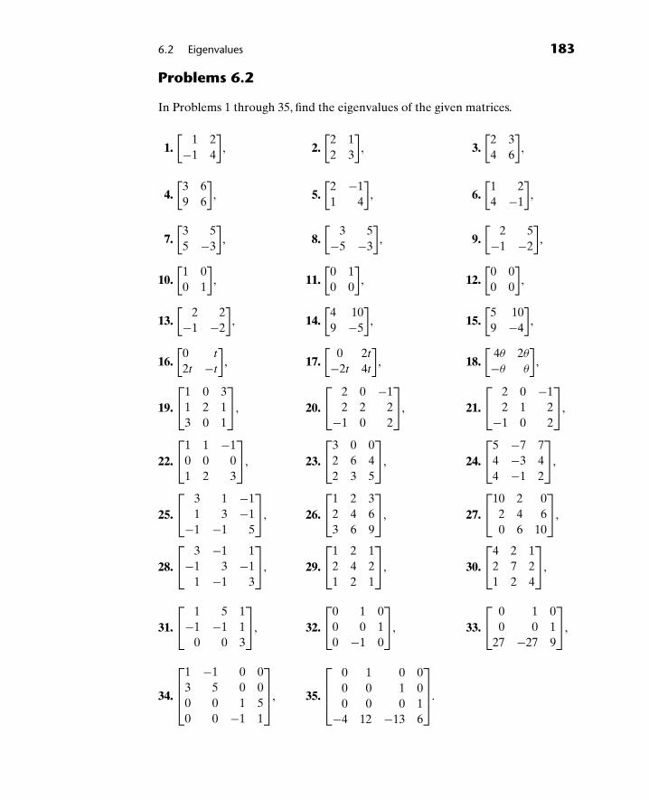
6.2 Eigenvalues 183
Problems 6.2
In Problems 1 through 35, find the eigenvalues of the given matrices.
1.[
1 2−1 4
], 2.
[2 12 3
], 3.
[2 34 6
],
4.[
3 69 6
], 5.
[2 −11 4
], 6.
[1 24 −1
],
7.[
3 55 −3
], 8.
[3 5
−5 −3
], 9.
[2 5
−1 −2
],
10.[
1 00 1
], 11.
[0 10 0
], 12.
[0 00 0
],
13.[
2 2−1 −2
], 14.
[4 109 −5
], 15.
[5 109 −4
],
16.[
0 t
2t −t
], 17.
[0 2t
−2t 4t
], 18.
[4θ 2θ
−θ θ
],
19.
⎡⎣1 0 3
1 2 13 0 1
⎤⎦, 20.
⎡⎣ 2 0 −1
2 2 2−1 0 2
⎤⎦, 21.
⎡⎣ 2 0 −1
2 1 2−1 0 2
⎤⎦,
22.
⎡⎣1 1 −1
0 0 01 2 3
⎤⎦, 23.
⎡⎣3 0 0
2 6 42 3 5
⎤⎦, 24.
⎡⎣5 −7 7
4 −3 44 −1 2
⎤⎦,
25.
⎡⎣ 3 1 −1
1 3 −1−1 −1 5
⎤⎦, 26.
⎡⎣1 2 3
2 4 63 6 9
⎤⎦, 27.
⎡⎣10 2 0
2 4 60 6 10
⎤⎦,
28.
⎡⎣ 3 −1 1
−1 3 −11 −1 3
⎤⎦, 29.
⎡⎣1 2 1
2 4 21 2 1
⎤⎦, 30.
⎡⎣4 2 1
2 7 21 2 4
⎤⎦,
31.
⎡⎣ 1 5 1
−1 −1 10 0 3
⎤⎦, 32.
⎡⎣0 1 0
0 0 10 −1 0
⎤⎦, 33.
⎡⎣ 0 1 0
0 0 127 −27 9
⎤⎦,
34.
⎡⎢⎢⎣
1 −1 0 03 5 0 00 0 1 50 0 −1 1
⎤⎥⎥⎦, 35.
⎡⎢⎢⎣
0 1 0 00 0 1 00 0 0 1
−4 12 −13 6
⎤⎥⎥⎦.

184 Chapter 6 Eigenvalues and Eigenvectors
36. Consider the matrix
C =
⎡⎢⎢⎢⎢⎣
0 1 0 · · · 00 0 1 · · · 0· · · · · · ·0 0 0 · · · 1
−a0 −a1 −a2 · · · −an−1
⎤⎥⎥⎥⎥⎦.
Use mathematical induction to prove that
det (C − λI) = (−1)n(λn + an−1λn−1 + · · · + a2λ
2 + a1λ + a0).
Deduce that the characteristic equation for this matrix is
λn + an−1λn−1 + · · · + a2λ
2 + a1λ + a0 = 0.
The matrix C is called the companion matrix for this characteristic equation.
37. Show that if λ is an eigenvalue of A, then kλ is an eigenvalue of kA, where k
denotes an arbitrary scalar.
38. Show that if λ �= 0 is an eigenvalue of A, then 1/λ is an eigenvalue of A−1,providing the inverse exists.
39. Show that if λ is an eigenvalue of A, then it is also an eigenvalue of AT.
6.3 Eigenvectors
To each distinct eigenvalue of a matrix A there will correspond at least oneeigenvector which can be found by solving the appropriate set of homogeneousequations. If an eigenvalue λi is substituted into (2), the corresponding eigenvectorxi is the solution of
(A − λiI)xi = 0. (6)
Example 1 Find the eigenvectors of
A =[
1 24 3
].
Solution The eigenvalues of A have already been found to be λ1 = −1, λ2 = 5(see Example 1 of Section 6.2). We first calculate the eigenvectors correspondingto λ1. From (6),
(A − (−1)I)x1 = 0. (7)

6.3 Eigenvectors 185
If we designate the unknown vector x1 by[x1y1
],
Eq. (7) becomes {[1 24 3
]+[
1 00 1
]}[x1y1
]=[
00
]or [
2 24 4
] [x1y1
]=[
00
].
or, equivalently,
2x1 + 2y1 = 0,
4x1 + 4y1 = 0.
A nontrivial solution to this set of equations is x1 = −y1, y1 arbitrary; hence, theeigenvector is
x1 =[x1y1
]=[−y1
y1
]= y1
[−11
], y1 arbitrary.
By choosing different values of y1, different eigenvectors for λ1 = −1 can beobtained. Note, however, that any two such eigenvectors would be scalar mul-tiples of each other, hence linearly dependent. Thus, there is only one linearlyindependent eigenvector corresponding to λ1 = −1. For convenience we choosey1 = 1, which gives us the eigenvector
x1 =[−1
1
].
Many times, however, the scalar y1 is chosen in such a manner that the resultingeigenvector becomes a unit vector. If we wished to achieve this result for the abovevector, we would have to choose y1 = 1/
√2.
Having found an eigenvector corresponding to λ1 = −1, we proceed to find aneigenvector x2 corresponding to λ2 = 5. Designating the unknown vector x2 by[
x2y2
]
and substituting it with λ2 into (6), we obtain{[1 24 3
]− 5
[1 00 1
]}[x2y2
]=[
00
],
or [− 4 24 −2
] [x2y2
]=[
00
],

186 Chapter 6 Eigenvalues and Eigenvectors
or, equivalently,
−4x2 + 2y2 = 0,
4x2 − 2y2 = 0.
A nontrivial solution to this set of equations is x2 = 12y2, where y2 is arbitrary;
hence
x2 =[x2y2
]=[y2/2y2
]= y2
[12
1
].
For convenience, we choose y2 = 2, thus
x2 =[
12
].
In order to check whether or not x2 is an eigenvector corresponding to λ2 = 5,we need only check if Ax2 = λ2x2:
Ax2 =[
1 24 3
] [12
]=[
510
]= 5
[12
]= λ2x2.
Again note that x2 is not unique! Any scalar multiple of x2 is also an eigenvectorcorresponding to λ2. However, in this case, there is just one linearly independenteigenvector corresponding to λ2. �
Example 2 Find the eigenvectors of
A =⎡⎣2 0 0
0 2 50 −1 −2
⎤⎦.
Solution By using the method of the previous section, we find the eigenvaluesto be λ1 = 2, λ2 = i, λ3 = −i. We first calculate the eigenvectors corresponding toλ1 = 2. Designate x1 by ⎡
⎣x1y1z1
⎤⎦.
Then (6) becomes
⎧⎨⎩⎡⎣2 0 0
0 2 50 −1 −2
⎤⎦− 2
⎡⎣1 0 0
0 1 00 0 1
⎤⎦⎫⎬⎭⎡⎣x1
y1z1
⎤⎦ =
⎡⎣0
00
⎤⎦,
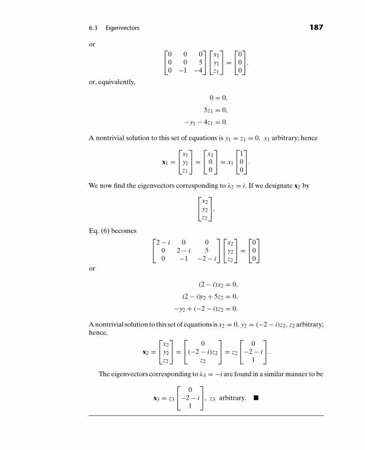
6.3 Eigenvectors 187
or ⎡⎣0 0 0
0 0 50 −1 −4
⎤⎦⎡⎣x1
y1z1
⎤⎦ =
⎡⎣0
00
⎤⎦,
or, equivalently,
0 = 0,
5z1 = 0,
−y1 − 4z1 = 0.
A nontrivial solution to this set of equations is y1 = z1 = 0, x1 arbitrary; hence
x1 =⎡⎣x1
y1z1
⎤⎦ =
⎡⎣x1
00
⎤⎦ = x1
⎡⎣1
00
⎤⎦.
We now find the eigenvectors corresponding to λ2 = i. If we designate x2 by⎡⎣x2
y2z2
⎤⎦,
Eq. (6) becomes ⎡⎣2 − i 0 0
0 2 − i 50 −1 −2 − i
⎤⎦⎡⎣x2
y2z2
⎤⎦ =
⎡⎣0
00
⎤⎦
or
(2 − i)x2 = 0,
(2 − i)y2 + 5z2 = 0,
−y2 + (−2 − i)z2 = 0.
A nontrivial solution to this set of equations is x2 = 0, y2 = (−2 − i)z2, z2 arbitrary;hence,
x2 =⎡⎣x2
y2z2
⎤⎦ =
⎡⎣ 0
(−2 − i)z2z2
⎤⎦ = z2
⎡⎣ 0
−2 − i
1
⎤⎦.
The eigenvectors corresponding to λ3 = −i are found in a similar manner to be
x3 = z3
⎡⎣ 0
−2 − i
1
⎤⎦, z3 arbitrary. �

188 Chapter 6 Eigenvalues and Eigenvectors
It should be noted that even if a mistake is made in finding the eigenvalues ofa matrix, the error will become apparent when the eigenvectors corresponding tothe incorrect eigenvalue are found. For instance, suppose that λ1 in Example 2 wascalculated erroneously to be 3. If we now try to find x1 we obtain the equations.
−x1 = 0,
−y1 + 5z1 = 0,
−y1 − 5z1 = 0.
The only solution to this set of equations is x1 = y1 = z1 = 0, hence
x1 =⎡⎣0
00
⎤⎦.
However, by definition, an eigenvector cannot be the zero vector. Since everyeigenvalue must have a corresponding eigenvector, there is a mistake. A quickcheck shows that all the calculations above are valid, hence the error must lie inthe value of the eigenvalue.
Problems 6.3
In Problems 1 through 23, find an eigenvector corresponding to each eigenvalueof the given matrix.
1.[
1 2−1 4
], 2.
[2 12 3
], 3.
[2 34 6
],
4.[
3 69 6
], 5.
[1 24 −1
], 6.
[3 55 −3
],
7.[
3 5−5 −3
], 8.
[2 5
−1 −2
], 9.
[2 2
−1 −2
],
10.[
4 109 −5
], 11.
[0 t
2t −t
], 12.
[4θ 2θ
−θ θ
],
13.
⎡⎣1 0 3
1 2 13 0 1
⎤⎦, 14.
⎡⎣ 2 0 −1
2 2 2−1 0 2
⎤⎦, 15.
⎡⎣ 3 0 −1
2 3 2−1 0 3
⎤⎦,
16.
⎡⎣3 0 0
2 6 42 3 5
⎤⎦, 17.
⎡⎣5 −7 7
4 −3 44 −1 2
⎤⎦, 18.
⎡⎣ 3 1 −1
1 3 −1−1 −1 5
⎤⎦,

6.3 Eigenvectors 189
19.
⎡⎣ 1 5 1
−1 −1 10 0 3
⎤⎦, 20.
⎡⎣0 1 0
0 0 10 −1 0
⎤⎦, 21.
⎡⎣3 2 1
0 4 00 1 5
⎤⎦,
22.
⎡⎢⎢⎣
1 −1 0 03 5 0 00 0 1 40 0 1 1
⎤⎥⎥⎦, 23.
⎡⎢⎢⎣
2 4 2 −20 1 0 00 3 3 −10 2 0 4
⎤⎥⎥⎦.
24. Find unit eigenvectors (i.e., eigenvectors whose magnitudes equal unity) forthe matrix in Problem 1.
25. Find unit eigenvectors for the matrix in Problem 2.
26. Find unit eigenvectors for the matrix in Problem 3.
27. Find unit eigenvectors for the matrix in Problem 13.
28. Find unit eigenvectors for the matrix in Problem 14.
29. Find unit eigenvectors for the matrix in Problem 16.
30. A nonzero vector x is a left eigenvector for a matrix A if there exists a scalar λ
such that xA = λx. Find a set of left eigenvectors for the matrix in Problem 1.
31. Find a set of left eigenvectors for the matrix in Problem 2.
32. Find a set of left eigenvectors for the matrix in Problem 3.
33. Find a set of left eigenvectors for the matrix in Problem 4.
34. Find a set of left eigenvectors for the matrix in Problem 13.
35. Find a set of left eigenvectors for the matrix in Problem 14.
36. Find a set of left eigenvectors for the matrix in Problem 16.
37. Find a set of left eigenvectors for the matrix in Problem 18.
38. Prove that if x is a right eigenvector of a symmetric matrix A, then xT is a lefteigenvector of A.
39. A left eigenvector for a given matrix is known to be [1 1]. Find another lefteigenvector for the same matrix satisfying the property that the sum of thevector components must equal unity.
40. A left eigenvector for a given matrix is known to be [2 3]. Find another lefteigenvector for the same matrix satisfying the property that the sum of thevector components must equal unity.
41. A left eigenvector for a given matrix is known to be [1 2 5]. Find anotherleft eigenvector for the same matrix satisfying the property that the sum ofthe vector components must equal unity.
42. A Markov chain (see Problem 16 of Section 1.1 and Problem 16 of Section 1.6)is regular if some power of the transition matrix contains only positive ele-ments. If the matrix itself contains only positive elements then the power

190 Chapter 6 Eigenvalues and Eigenvectors
is one, and the matrix is automatically regular. Transition matrices that areregular always have an eigenvalue of unity. They also have limiting distribu-tion vectors denoted by x(∞), where the ith component of x(∞) represents theprobability of an object being in state i after a large number of time periodshave elapsed. The limiting distribution x(∞) is a left eigenvector of the tran-sition matrix corresponding to the eigenvalue of unity, and having the sum ofits components equal to one.
(a) Find the limiting distribution vector for the Markov chain described inProblem 16 of Section 1.1.
(b) Ultimately, what is the probability that a family will reside in the city?
43. Find the limiting distribution vector for the Markov chain described in Prob-lem 17 of Section 1.1. What is the probability of having a Republican mayorover the long run?
44. Find the limiting distribution vector for the Markov chain described in Prob-lem 18 of Section 1.1. What is the probability of having a good harvest overthe long run?
45. Find the limiting distribution vector for the Markov chain described in Prob-lem 19 of Section 1.1. Ultimately, what is the probability that a person will useBrand Y?
6.4 Properties of Eigenvalues and Eigenvectors
Definition 1 The trace of a matrix A, designated by tr(A), is the sum of theelements on the main diagonal.
Example 1 Find the tr(A) if
A =⎡⎣3 −1 2
0 4 11 −1 −5
⎤⎦.
Solution tr(A) = 3 + 4 + (−5) = 2. �
Property 1 The sum of the eigenvalues of a matrix equals the trace of the matrix.
Proof. See Problem 20.
Property 1 provides us with a quick and useful procedure for checkingeigenvalues.
Example 2 Verify Property 1 for
A =[
11 3−5 −5
].

6.4 Properties of Eigenvalues and Eigenvectors 191
Solution The eigenvalues of A are λ1 = 10, λ2 = −4.
tr(A) = 11 + (−5) = 6 = λ1 + λ2. �
Property 2 A matrix is singular if and only if it has a zero eigenvalue.
Proof. A matrix A has a zero eigenvalue if and only if det(A − 0I) = 0, or (since0I = 0) if and only if det(A) = 0. But det(A) = 0 if and only if A is singular, thus,the result is immediate.
Property 3 The eigenvalues of an upper (or lower) triangular matrix are theelements on the main diagonal.
Proof. See Problem 15.
Example 3 Find the eigenvalues of
A =⎡⎣1 0 0
2 1 03 4 −1
⎤⎦.
Solution Since A is lower triangular, the eigenvalues must be λ1 = λ2 = 1,λ3 = −1. �
Property 4 If λ is an eigenvalue of A and if A is invertible, then 1/λ is aneigenvalue of A−1.
Proof. Since A is invertible, Property 2 implies that λ �= 0; hence 1/λ exists.Since λ is an eigenvalue of A there must exist an eigenvector x such that Ax = λx.Premultiplying both sides of this equation by A−1, we obtain
x = λA−1x
or, equivalently, A−1x = (1/λ)x. Thus, 1/λ is an eigenvalue of A−1.
OBSERVATION 1 If x is an eigenvector of A corresponding to the eigenvalue λ
and if A is invertible, then x is an eigenvector of A−1 corresponding to theeigenvalue 1/λ.
Property 5 If λ is an eigenvalue of A, then αλ is an eigenvalue of αA where α isany arbitrary scalar.
Proof. If λ is an eigenvalue of A, then there must exist an eigenvector x such thatAx = λx. Multiplying both sides of this equation by α, we obtain (αA)x = (αλ)xwhich implies Property 5.

192 Chapter 6 Eigenvalues and Eigenvectors
OBSERVATION 2 If x is an eigenvector of A corresponding to the eigenvalue λ,then x is an eigenvector of αA corresponding to eigenvalue αλ.
Property 6 If λ is an eigenvalue of A, then λk is an eigenvalue of Ak, for anypositive integer k.
Proof. We prove the result for the special cases k = 2 and k equals 3. Other casesare handled by mathematical induction. (See Problem 16.) If λ is an eigenvalueof A, there must exist an eigenvector x such that Ax = λx. Then,
A2x = A(Ax) = A(λx) = λ(Ax) = λ(λx) = λ2x,
which implies that λ2 is an eigenvalue of A2. As a result, we also have that
A3x = A(A2x) = A(λ2x) = λ2(Ax) = λ2(λx) = λ3x,
which implies that λ3 is an eigenvalue of A3.
OBSERVATION 3 If x is an eigenvector of A corresponding to the eigenvalue λ,then x is an eigenvector Ak corresponding to the eigenvalue λk, for any positiveinteger k.
Property 7 If λ is an eigenvalue of A, then for any scalar c, λ − c is an eigenvalueof A − cI.
Proof. If λ is an eigenvalue of A, then there exists an eigenvector x such thatAx = λx. Consequently,
Ax − cx = λx − cx,
or
(A − cI)x = (λ − c)x.
Thus, λ − c is an eigenvalue of A − cI.
OBSERVATION 4 If x is an eigenvector of A corresponding to the eigenvalue λ,then x is an eigenvector A − cI corresponding to the eigenvalue λ − c.
Property 8 If λ is an eigenvalue of A, then λ is an eigenvalue of AT.
Proof. Since λ is an eigenvalue of A, det(A − λI) = 0. Hence
0 = ∣∣A − λI∣∣ = ∣∣(AT)T − λIT
∣∣ {Property 1 (Section 1.4)
= ∣∣(AT − λI)T∣∣ {
Property 3 (Section 1.4)
= ∣∣AT − λI∣∣ {
Property 7 (Section 5.3)
Thus, det(AT − λI
) = 0, which implies that λ is an eigenvalue of AT.

6.4 Properties of Eigenvalues and Eigenvectors 193
Property 9 The product of the eigenvalues (counting multiplicity) of a matrixequals the determinant of the matrix.
Proof. See Problem 21.
Example 4 Verify Property 9 for the matrix A given in Example 2:
Solution For this A, λ1 = 10, λ2 = −4, det(A) = −55 + 15 = −40 = λ1λ2. �
Problems 6.4
1. One eigenvalue of the matrix
A =[
8 23 3
]
is known to be 2. Determine the second eigenvalue by inspection.
2. One eigenvalue of the matrix
A =[
8 33 2
]
is known to be 0.7574, rounded to four decimal places. Determine the secondeigenvalue by inspection.
3. Two eigenvalues of a 3 × 3 matrix are known to be 5 and 8. What can be saidabout the remaining eigenvalue if the trace of the matrix is −4?
4. Redo Problem 3 if the determinant of the matrix is −4 instead of its trace.
5. The determination of a 4 × 4 matrix A is 144 and two of its eigenvalues areknown to be −3 and 2. What can be said about the remaining eigenvalues?
6. A 2 × 2 matrix A is known to have the eigenvalues−3 and 4. What are the eigen-values of (a) 2A, (b) 5A, (c) A − 3I, and (d) A + 4I?
7. A 3 × 3 matrix A is known to have the eigenvalues −2, 2, and 4. What are theeigenvalues of (a) A2, (b) A3, (c) −3A, and (d) A + 3I?
8. A 2 × 2 matrix A is known to have the eigenvalues −1 and 1. Find a matrix interms of A that has for its eigenvalues:
(a) −2 and 2, (b) −5 and 5,(c) 1 and 1, (d) 2 and 4.
9. A 3 × 3 matrix A is known to have the eigenvalues 2, 3, and 4. Find a matrixin terms of A that has for its eigenvalues:
(a) 4, 6, and 8, (b) 4, 9, and 16,(c) 8, 27, and 64, (d) 0, 1, and 2.

194 Chapter 6 Eigenvalues and Eigenvectors
10. Verify Property 1 for
A =[
12 16−3 −7
].
11. Verify Property 2 for
A =⎡⎣ 1 3 6
−1 2 −12 1 7
⎤⎦.
12. Show that if λ is an eigenvalue of A, then it is also an eigenvalue for S−1ASfor any nonsingular matrix S.
13. Show by example that, in general, an eigenvalue of A + B is not the sum ofan eigenvalue of A with an eigenvalue of B.
14. Show by example that, in general, an eigenvalue of AB is not the product ofan eigenvalue of A with an eigenvalue of B.
15. Prove Property 3.
16. Use mathematical induction to complete the proof of Property 6.
17. The determinant of A − λI is known as the characteristic polynomial of A.For an n × n matrix A, it has the form
det (A − λI) = (−1)n(λn + an−1λn−1 + an−2λ
n−2 + · · · + a2λ2 + a1λ + a0),
where an−1, an−2, . . . , a2, a1, a0 are constants that depend on the elements ofA. Show that (−1)na0 = det (A).
18. (Problem 17 continued) Convince yourself by considering arbitrary 3 × 3 and4 × 4 matrices that an−1 = tr(A).
19. Assume that A is an n × n matrix with eigenvalues λ1, λ2, . . . , λn, wheresome or all of the eigenvalues may be equal. Since each eigenvalueλi(i = 1, 2, . . . , n) is a root of the characteristic polynomial, (λ − λi) mustbe a factor of that polynomial. Deduce that
det (A − λI) = (−1)n(λ − λ1)(λ − λ2) · · · (λ − λn).
20. Use the results of Problems 18 and 19 to prove Property 1.
21. Use the results of Problems 17 and 19 to prove Property 9.
22. Show, by example, that an eigenvector of A need not be an eigenvector of AT.
23. Prove that an eigenvector of A is a left eigenvector of AT.
6.5 Linearly Independent Eigenvectors
Since every eigenvalue has an infinite number of eigenvectors associated withit (recall that if x is an eigenvector, then any scalar multiple of x is also an

6.5 Linearly Independent Eigenvectors 195
eigenvector), it becomes academic to ask how many different eigenvectors cana matrix have? The answer is clearly an infinite number. A more revealing ques-tion is how many linearly independent eigenvectors can a matrix have? Theorem4 of Section 2.6 provides us with a partial answer.
Theorem 1 In an n-dimensional vector space, every set of n + 1 vectors islinearly dependent.
Therefore, since all of the eigenvectors of an n × n matrix must be n-dimensional (why?), it follows from Theorem 1 that an n × n matrix can haveat most n linearly independent eigenvectors. The following three examples shedmore light on the subject.
Example 1 Find the eigenvectors of
A =⎡⎣2 1 0
0 2 10 0 2
⎤⎦.
Solution The eigenvalues of A are λ1 = λ2 = λ3 = 2, therefore λ = 2 is aneigenvalue of multiplicity 3. If we designate the unknown eigenvector x by
⎡⎣x
y
z
⎤⎦,
then Eq. (6) gives rise to the three equations
y = 0,
z = 0,
0 = 0.
Thus, y = z = 0 and x is arbitrary; hence
x =⎡⎣x
y
z
⎤⎦ =
⎡⎣x
00
⎤⎦ = x
⎡⎣1
00
⎤⎦.
Setting x = 1, we see that λ = 2 generates only one linearly independent eigen-vector,
x =⎡⎣1
00
⎤⎦. �

196 Chapter 6 Eigenvalues and Eigenvectors
Example 2 Find the eigenvectors of
A =⎡⎣2 1 0
0 2 00 0 2
⎤⎦.
Solution Again, the eigenvalues are λ1 = λ2 = λ3 = 2, therefore λ = 2 is aneigenvalue of multiplicity 3. Designate the unknown eigenvector x by
⎡⎣x
y
z
⎤⎦.
Equation (6) now gives rise to the equations
y = 0,
0 = 0,
0 = 0.
Thus, y = 0 and both x and z are arbitrary; hence
x =⎡⎣x
y
z
⎤⎦ =
⎡⎣x
0z
⎤⎦ =
⎡⎣x
00
⎤⎦+
⎡⎣0
0z
⎤⎦ = x
⎡⎣1
00
⎤⎦+ z
⎡⎣0
01
⎤⎦.
Since x and z can be chosen arbitrarily, we can first choose x = 1 and z = 0 toobtain
x1 =⎡⎣1
00
⎤⎦
and then choose x = 0 and z = 1 to obtain
x2 =⎡⎣0
01
⎤⎦.
x1 and x2 can easily be shown to be linearly independent vectors, hence we seethat λ = 2 generates the two linearly independent eigenvectors
⎡⎣1
00
⎤⎦ and
⎡⎣0
01
⎤⎦. �

6.5 Linearly Independent Eigenvectors 197
Example 3 Find the eigenvectors of
A =⎡⎣2 0 0
0 2 00 0 2
⎤⎦.
Solution Again the eigenvalues are λ1 = λ2 = λ3 = 2 so again λ = 2 is aneigenvalue of multiplicity three. Designate the unknown eigenvector x by
⎡⎣x
y
z
⎤⎦.
Equation (6) gives rise to the equations
0 = 0,
0 = 0,
0 = 0,
Thus, x, y, and z are all arbitrary; hence
x =⎡⎣x
y
z
⎤⎦ =
⎡⎣x
00
⎤⎦+
⎡⎣0
y
0
⎤⎦+
⎡⎣0
0z
⎤⎦ = x
⎡⎣1
00
⎤⎦+ y
⎡⎣0
10
⎤⎦+ z
⎡⎣0
01
⎤⎦.
Since x, y, and z can be chosen arbitrarily, we can first choose x = 1, y = z = 0,then choose x = z = 0, y = 1 and finally choose y = x = 0, z = 1 to generate thethree linearly independent eigenvectors
⎡⎣1
00
⎤⎦,
⎡⎣0
10
⎤⎦,
⎡⎣0
01
⎤⎦.
In this case we see that three linearly independent eigenvectors are generatedby λ = 2. (Note that, from Theorem 1, this is the maximal number that could begenerated.) �
The preceding examples are illustrations of
Theorem 2 If λ is an eigenvalue of multiplicity k of an n × n matrix A, thenthe number of linearly independent eigenvectors of A associated with λ is given byρ = n − r(A − λI). Furthermore, 1 ≤ ρ ≤ k.

198 Chapter 6 Eigenvalues and Eigenvectors
Proof. Let x be an n-dimensional vector. If x is an eigenvector, then it mustsatisfy the vector equation Ax = λx or, equivalently, (A − λI)x = 0. This system ishomogeneous, hence consistent, so by Theorem 2 of Section 2.7, we have that thesolution vector x will be in terms of n − r(A − λI) arbitrary unknowns. Since theseunknowns can be picked independently of each other, it follows that the number oflinearly independent eigenvectors of A associated with λ is also ρ = n − r(A − λI).We defer a proof that 1 ≤ ρ ≤ k until Chapter 9.
In Example 1, A is 3 × 3; hence n = 3, and r(A − 2I) = 2. Thus, there should be3 − 2 = 1 linearly independent eigenvector associated with λ = 2 which is indeedthe case. In Example 2, once again n = 3 but r(A − 2I) = 1. Thus, there shouldbe 3 − 1 = 2 linearly independent eigenvectors associated with λ = 2 which alsois the case.
The next theorem gives the relationship between eigenvectors that correspondto different eigenvalues.
Theorem Eigenvectors corresponding to distinct (that is, different) eigenvaluesare linearly independent.
Proof. For the sake of clarity, we consider the case of three distinct eigenvectorsand leave the more general proof as an exercise (see Problem 17). Therefore,let λ1, λ2, λ3, be distinct eigenvalues of the matrix A and let x1, x2, x3 be theassociated eigenvectors. That is
Ax1 = λ1x1,
Ax2 = λ2x2,
Ax3 = λ3x3,
(8)
and λ1 �= λ2 �= λ3 �= λ1.Since we want to show that x1, x2, x3 are linearly independent, we must show
that the only solution to
c1x1 + c2x2 + c3x3 = 0 (9)
is c1 = c2 = c3 = 0. By premultiplying (9) by A, we obtain
c1Ax1 + c2Ax2 + c3Ax3 = A • 0 = 0.
It follows from (8), therefore, that
c1λ1x1 + c2λ2x2 + c3λ3x3 = 0. (10)
By premultiplying (10) by A and again using (8), we obtain
c1λ21x1 + c2λ
22x2 + c3λ
23x3 = 0. (11)
Equations (9)–(11) can be written in the matrix form⎡⎢⎣1 1 1
λ1 λ2 λ3
λ21 λ2
2 λ23
⎤⎥⎦⎡⎢⎣c1x1
c2x2
c3x3
⎤⎥⎦ =
⎡⎢⎣0
0
0
⎤⎥⎦.

6.5 Linearly Independent Eigenvectors 199
Define
B =⎡⎢⎣
1 1 1λ1 λ2 λ3
λ21 λ2
2 λ23
⎤⎥⎦.
It can be shown that det(B) = (λ2 − λ1)(λ3 − λ2)(λ3 − λ1). Thus, since all theeigenvalues are distinct, det (B) �= 0 and B is invertible. Therefore,
⎡⎣c1x1
c2x2c3x3
⎤⎦ = B−1
⎡⎣0
00
⎤⎦ =
⎡⎣0
00
⎤⎦
or ⎡⎢⎣c1x1 = 0
c2x2 = 0c3x3 = 0
⎤⎥⎦ (12)
But since x1, x2, x3 are eigenvectors, they are nonzero, therefore, it follows from(12) that c1 = c2 = c3 = 0. This result together with (9) implies Theorem 3.
Theorems 2 and 3 together completely determine the number of linearlyindependent eigenvectors of a matrix.
Example 4 Find a set of linearly independent eigenvectors for
A =⎡⎣1 0 0
4 3 24 2 3
⎤⎦.
Solution The eigenvalues of A are λ1 = λ2 = 1, and λ3 = 5. For this matrix,n = 3 and r(A − 1I) = 1, hencen − r(A − 1I) = 2. Thus, fromTheorem 2, we knowthat A has two linearly independent eigenvectors corresponding to λ = 1 and onelinearly independent eigenvector corresponding to λ = 5 (why?). Furthermore,Theorem 3 guarantees that the two eigenvectors corresponding to λ = 1 will belinearly independent of the eigenvector corresponding to λ = 5 and vice versa. Itonly remains to produce these vectors.
For λ = 1, the unknown vector
x1 =
⎡⎢⎢⎣
x1
y1
z1
⎤⎥⎥⎦

200 Chapter 6 Eigenvalues and Eigenvectors
must satisfy the vector equation (A − 1I)x1 = 0, or equivalently, the set ofequations
0 = 0,
4x1 + 2y1 + 2z1 = 0,
4x1 + 2y1 + 2z1 = 0.
A solution to this equation is z1 = −2x1 − y1, x1, and y1 arbitrary. Thus,
x1 =⎡⎢⎣x1
y1
z1
⎤⎥⎦ =
⎡⎢⎣ x1
y1
−2x1 − y1
⎤⎥⎦ = x1
⎡⎢⎣ 1
0
−2
⎤⎥⎦+ y1
⎡⎢⎣ 0
1
−1
⎤⎥⎦.
By first choosing x1 = 1, y1 = 0 and then x1 = 0, y1 = 1, we see that λ = 1generates the two linearly independent eigenvectors
⎡⎢⎣ 1
0
−2
⎤⎥⎦,
⎡⎢⎣ 0
1
−1
⎤⎥⎦.
An eigenvector corresponding to λ3 = 5 is found to be
⎡⎢⎣0
1
1
⎤⎥⎦.
Therefore, A possesses the three linearly independent eigenvectors,
⎡⎢⎣ 1
0
−2
⎤⎥⎦,
⎡⎢⎣ 0
1
−1
⎤⎥⎦,
⎡⎢⎣0
1
1
⎤⎥⎦. �
Problems 6.5
In Problems 1–16 find a set of linearly independent eigenvectors for the givenmatrices.
1.[
2 −11 4
], 2.
[3 10 3
], 3.
[3 00 3
],

6.6 Power Methods 201
4.
⎡⎣2 1 1
0 1 01 1 2
⎤⎦, 5.
⎡⎣2 1 1
0 1 01 2 2
⎤⎦, 6.
⎡⎣ 2 0 −1
2 1 −2−1 0 2
⎤⎦,
7.
⎡⎣1 1 −1
0 0 01 2 3
⎤⎦, 8.
⎡⎣1 2 3
2 4 63 6 9
⎤⎦, 9.
⎡⎣ 3 −1 1
−1 3 −11 −1 3
⎤⎦,
10.
⎡⎣ 0 1 0
0 0 127 −27 9
⎤⎦, 11.
⎡⎣0 1 0
0 0 11 −3 3
⎤⎦, 12.
⎡⎣4 2 1
2 7 21 2 4
⎤⎦,
13.
⎡⎢⎢⎣
0 1 0 00 0 1 00 0 0 1
−1 4 −6 4
⎤⎥⎥⎦, 14.
⎡⎢⎢⎣
1 0 0 00 0 1 00 0 0 10 1 −3 3
⎤⎥⎥⎦,
15.
⎡⎢⎢⎣
1 0 0 01 2 1 11 1 2 11 1 1 2
⎤⎥⎥⎦, 16.
⎡⎢⎢⎣
3 1 1 20 3 1 10 0 2 00 0 0 2
⎤⎥⎥⎦.
17. The Vandermonde determinant∣∣∣∣∣∣∣∣∣∣∣∣∣∣∣
1 1 · · · 1x1 x2 · · · xn
x21 x2
2 · · · x2n
......
...
xn−11 xn−1
2 . . . xn−1n
∣∣∣∣∣∣∣∣∣∣∣∣∣∣∣is known to equal the product
(x2 − x1)(x3 − x2)(x3 − x1)(x4 − x3)(x4 − x2) · · · (xn − x1).
Using this result, prove Theorem 3 for n distinct eigenvalues.
6.6 Power Methods
The analytic methods described in Sections 6.2 and 6.3 are impractical for calculat-ing the eigenvalues and eigenvectors of matrices of large order. Determining thecharacteristic equations for such matrices involves enormous effort, while findingits roots algebraically is usually impossible. Instead, iterative methods which lend

202 Chapter 6 Eigenvalues and Eigenvectors
themselves to computer implementation are used. Ideally, each iteration yieldsa new approximation, which converges to an eigenvalue and the correspondingeigenvetor.
The dominant eigenvalue of a matrix is the one having largest absolute val-ues. Thus, if the eigenvalues of a matrix are 2, 5, and −13, then −13 is thedominant eigenvalue because it is the largest in absolute value. The powermethod is an algorithm for locating the dominant eigenvalue and a correspond-ing eigenvector for a matrix of real numbers when the following two conditionsexist:
Condition 1. The dominant eigenvalue of a matrix is real (not complex) and isstrictly greater in absolute values than all other eigenvalues.
Condition 2. If the matrix has order n × n, then it possesses n linearlyindependent eigenvectors.
Denote the eigenvalues of a given square matrix A satisfying Conditions 1and 2 by λ1, λ2, . . . , λn, and a set of corresponding eigenvectors by v1, v2, . . . , vn,respectively. Assume the indexing is such that
|λ1| > |λ2| ≥ |λ3| ≥ · · · ≥ |λn|.
Any vector x0 can be expressed as a linear combination of the eigenvectors of A,so we may write
x0 = c1v1 + c2v2 + · · · + cnvn.
Multiplying this equation by Ak, for some large, positive integer k, we get
Akx0 = Ak(c1v1 + c2v2 + · · · + cnvn)
= c1Akv1 + c2Akv2 + · · · + cnAkvn.
It follows from Property 6 and Observation 3 of Section 6.4 that
Akx0 = c1λk1v1 + c2λ
k2v2 + · · · + cnλ
knvn
= λk1
[c1v1 + c2
(λ2
λ1
)k
v2 + · · · + cn
(λn
λ1
)k
vn
]
≈ λk1c1v1 for large k.

6.6 Power Methods 203
This last pseudo-equality follows from noting that each quotient of eigenvalues isless than unity in absolute value, as a result of indexing the first eigenvalue as thedominant one, and therefore tends to zero as that quotient is raised to successivelyhigher powers.
Thus, Akx0 approaches a scalar multiple of v1. But any nonzero scalar multipleof an eigenvector is itself an eigenvector, so Akx0 approaches an eigenvector of Acorresponding to the dominant eigenvalue, providing c1 is not zero. The scalar c1will be zero only if x0 is a linear combination of {v2, v3, . . . , vn}.
The power method begins with an initial vector x0, usually the vector havingall ones for its components, and then iteratively calculates the vectors
x1 = Ax0,
x2 = Ax1 = A2x0,
x3 = Ax2 = A3x0,
...
xk = Axk−1 = Akx0.
As k gets larger, xk approaches an eigenvector of A corresponding to its dominanteigenvalue.
We can even determine the dominant eigenvalue by scaling appropriately. If k
is large enough so that xk is a good approximation to the eigenvector, say to withinacceptable roundoff error, then it follows from Eq. (1) that
Axk = λ1xk.
If xk is scaled so that its largest component is unity, then the component of xk+1 =Axk = λ1xk having the largest absolute value must be λ1.
We can now formalize the power method. Begin with an initial guess x0 forthe eigenvector, having the property that its largest component in absolute valueis unity. Iteratively, calculate x1, x2, x3, . . . by multiplying each successive iterateby A, the matrix of interest. Each time xk(k = 1, 2, 3, . . .) is computed, identifyits dominant component and divide each component by it. Redefine this scaledvector as the new xk. Each xk is an estimate of an eigenvector for A and eachdominant component is an estimate for the associated eigenvalue.
Example 1 Find the dominant eigenvalue, and a corresponding eigenvector for
A =[
1 24 3
].
Solution We initialize x0 = [1 1]T. Then

204 Chapter 6 Eigenvalues and Eigenvectors
First Iteration
x1 = Ax0 =[
1 24 3
] [11
]=[
37
],
λ ≈ 7,
x1 ← 17
[3 7
]T = [0.428571 1]T
.
Second Iteration
x2 = Ax1 =[
1 24 3
] [0.428571
1
]=[
2.4285714.714286
],
λ ≈ 4.714286,
x2 ← 14.714286
[2.428571 4.714286
]T = [0.515152 1]T
.
Third Iteration
x3 = Ax2 =[
1 24 3
] [0.515152
1
]=[
2.5151525.060606
],
λ = 5.060606,
x3 ← 15.060606
[2.515152 5.060606]T = [0.497006 1]T .
Fourth Iteration
x4 = Ax3 =[
1 24 3
] [0.497006
1
]=[
2.4970064.988024
],
λ ≈ 4.988024,
x4 ← 14.988024
[2.497006 4.988024
]T = [0.500600 1]T
.
The method is converging to the eigenvalue 5 and its corresponding eigenvector[0.5 1
]T. �
Example 2 Find the dominant eigenvalue and a corresponding eigenvector for
A =⎡⎣ 0 1 0
0 0 118 −1 −7
⎤⎦.

6.6 Power Methods 205
Solution We initialize x0 = [1 1 1]T. Then
First Iteration
x1 = Ax0 = [1 1 10]T
,
λ ≈ 10,
x1 ← 110
[1 1 10
]T = [0.1 0.1 1]T
.
Second Iteration
x2 = Ax1 =⎡⎣ 0 1 0
0 0 118 −1 −7
⎤⎦⎡⎣0.1
0.11
⎤⎦ =
⎡⎣ 0.1
1−5.3
⎤⎦,
λ ≈ −5.3,
x2 ← 1−5.3
[0.1 1 −5.3
]T= [−0.018868 −0.188679 1
]T.
Third Iteration
x3 = Ax2 =⎡⎣ 0 1 0
0 0 118 −1 −7
⎤⎦⎡⎣−0.018868
−0.1886791
⎤⎦ =
⎡⎣−0.188679
1−7.150943
⎤⎦,
λ ≈ −7.150943,
x3 ← 1−7.150943
[−0.188679 1 −7.150943]T
= [0.026385 −0.139842 1
]T.
Continuing in this manner, we generateTable 6.1, where all entries are roundedto four decimal places. The algorithm is converging to the eigenvalue −6.405125and its corresponding eigenvector
[0.024376 −0.1561240 1
]T. �
Although effective when it converges, the power method has deficiencies. Itdoes not converge to the dominant eigenvalue when that eigenvalue is complex,and it may not converge when there are more than one equally dominant eigen-values (See Problem 12). Furthermore, the method, in general, cannot be used tolocate all the eigenvalues.
A more powerful numerical method is the inverse power method, which is thepower method applied to the inverse of a matrix. This, of course, adds anotherassumption: the inverse must exist, or equivalently, the matrix must not haveany zero eigenvalues. Since a nonsingular matrix and its inverse share identical

206 Chapter 6 Eigenvalues and Eigenvectors
Table 6.1Iteration Eigenvector components Eigenvalue
0 1.0000 1.0000 1.00001 0.1000 0.1000 1.0000 10.00002 −0.0189 −0.1887 1.0000 −5.30003 0.0264 −0.1398 1.0000 −7.15094 0.0219 −0.1566 1.0000 −6.38525 0.0243 −0.1551 1.0000 −6.44926 0.0242 −0.1561 1.0000 −6.40787 0.0244 −0.1560 1.0000 −6.40848 0.0244 −0.1561 1.0000 −6.4056
eigenvectors and reciprocal eigen- values (see Property 4 and Observation 1 ofSection 6.4), once we know the eigenvalues and eigenvectors of the inverse of amatrix, we have the analogous information about the matrix itself.
The power method applied to the inverse of a matrix A will generally convergeto the dominant eigenvalue of A−1. Its reciprocal will be the eigenvalue of Ahaving the smallest absolute value. The advantages of the inverse power methodare that it converges more rapidly than the power method, and if often can be usedto find all real eigenvalues of A; a disadvantage is that it deals with A−1, whichis laborious to calculate for matrices of large order. Such a calculation, however,can be avoided using LU decomposition.
The power method generates the sequence of vectors
xk = Axk−1.
The inverse power method will generate the sequence
xk = A−1xk−1,
which may be written as
Axk = xk−1.
We solve for the unknown vector xk using LU-decomposition (see Section 3.5).
Example 3 Use the inverse power method to find an eigenvalue for
A =[
2 12 3
].
Solution We initialize x0 = [1 1]T. The LU decomposition for A has A = LUwith
L =[
1 01 1
]and U =
[2 10 2
].
First Iteration. We solve the system LUx1 = x0 by first solving the systemLy = x0 for y, and then solving the system Ux1 = y for x1. Set y = [y1 y2]T and

6.6 Power Methods 207
x1 = [a b]T. The first system is
y1 + 0y2 = 1,
y1 + y2 = 1,
which has as its solution y1 = 1 and y2 = 0. The system Ux1 = y becomes
2a + b = 1,
2b = 0,
which admits the solution a = 0.5 and b = 0. Thus,
x1 = A−1x0 = [0.5 0]T ,
λ ≈ 0.5 (an approximation to an eigenvalue for A−1),
x1 ← 10.5
[0.5 0]T = [1 0]T .
Second Iteration. We solve the system LUx2 = x1 by first solving the systemLy = x1 for y, and then solving the system Ux2 = y for x2. Set y = [y1 y2]T andx2 = [a b]T. The first system is
y1 + 0y2 = 1,
y1 + y2 = 0,
which has as its solution y1 = 1 and y2 = −1. The system Ux2 = y becomes
2a + b = 1,
2b = −1,
which admits the solution a = 0.75 and b = −0.5. Thus,
x2 = A−1x1 = [0.75 −0.5]T,
λ ≈ 0.75,
x2 ← 10.75
[0.75 −0.5
]T = [1 −0.666667]T
.
Third Iteration. We first solve Ly = x2 to obtain y = [1 −1.666667]T, and then
Ux3 = y to obtain x3 = [0.916667 −0.833333]T. Then,
λ ≈ 0.916667
x3 ← 10.916667
[0.916667 −0.833333
]T = [1 −0.909091]T
.
Continuing, we converge to the eigenvalue 1 for A−1 and its reciprocal 1/1 = 1 forA. The vector approximations are converging to
[1 −1
]T, which is an eigenvectorfor both A−1 and A. �

208 Chapter 6 Eigenvalues and Eigenvectors
Example 4 Use the inverse power method to find an eigenvalue for
A =⎡⎣7 2 0
2 1 60 6 7
⎤⎦.
Solution We initialize x0 = [1 1 1]T. The LU decomposition for A has
A = LU with
L =⎡⎣ 1 0 0
0.285714 1 00 14 1
⎤⎦ and U =
⎡⎣7 2 0
0 0.428571 60 0 −77
⎤⎦ .
First Iteration
Set y = [y1 y2 y3]T and x1 = [a b c
]T. The first system is
y1 + 0y2 + 0y3 = 1,
0.285714y1 + y2 + 0y3 = 1,
0y1 + 14y2 + y3 = 1,
which has as its solution y1 = 1, and y2 = 0.714286, and y3 = −9. The systemUx1 = y becomes
7a + 2b = 1,
0.428571b + 6c = 0.714286,
−77c = −9,
which admits the solution a = 0.134199, b = 0.030303, and c = 0.116883. Thus,
x1 = A−1x0 = [0.134199 0.030303 0.116833]T
,
λ ≈ 0.134199 (an approximation to an eigenvalue for A−1),
x1 ← 10.134199
[0.134199 0.030303 0.116833
]T= [1 0.225806 0.870968
]T.
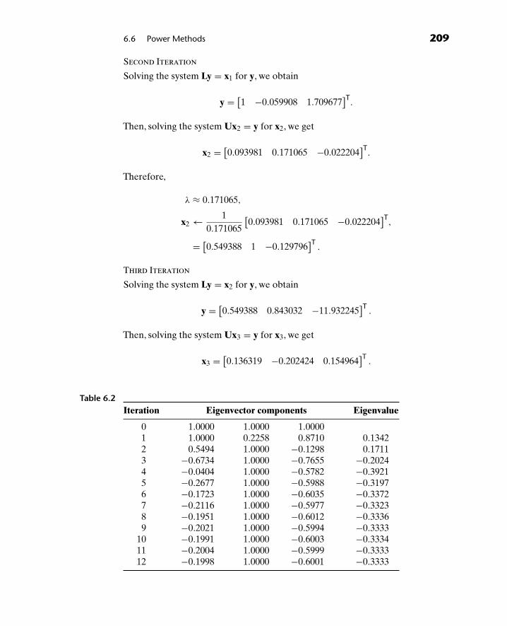
6.6 Power Methods 209
Second Iteration
Solving the system Ly = x1 for y, we obtain
y = [1 −0.059908 1.709677]T
.
Then, solving the system Ux2 = y for x2, we get
x2 = [0.093981 0.171065 −0.022204]T
.
Therefore,
λ ≈ 0.171065,
x2 ← 10.171065
[0.093981 0.171065 −0.022204
]T,
= [0.549388 1 −0.129796]T
.
Third Iteration
Solving the system Ly = x2 for y, we obtain
y = [0.549388 0.843032 −11.932245]T
.
Then, solving the system Ux3 = y for x3, we get
x3 = [0.136319 −0.202424 0.154964]T
.
Table 6.2Iteration Eigenvector components Eigenvalue
0 1.0000 1.0000 1.00001 1.0000 0.2258 0.8710 0.13422 0.5494 1.0000 −0.1298 0.17113 −0.6734 1.0000 −0.7655 −0.20244 −0.0404 1.0000 −0.5782 −0.39215 −0.2677 1.0000 −0.5988 −0.31976 −0.1723 1.0000 −0.6035 −0.33727 −0.2116 1.0000 −0.5977 −0.33238 −0.1951 1.0000 −0.6012 −0.33369 −0.2021 1.0000 −0.5994 −0.3333
10 −0.1991 1.0000 −0.6003 −0.333411 −0.2004 1.0000 −0.5999 −0.333312 −0.1998 1.0000 −0.6001 −0.3333

210 Chapter 6 Eigenvalues and Eigenvectors
Therefore,
λ ≈ −0.202424,
x3 ← 1−0.202424
[0.136319 −0.202424 0.154964
]T= [−0.673434 1 −0.765542
]T.
Continuing in this manner, we generateTable 6.2, where all entries are roundedto four decimal places. The algorithm is converging to the eigenvalue −1/3 forA−1 and its reciprocal −3 for A. The vector approximations are converging to[−0.2 1 − 0.6]T, which is an eigenvector for both A−1 and A. �
We can use Property 7 and Observation 4 of Section 6.4 in conjunction withthe inverse power method to develop a procedure for finding all eigenvalues anda set of corresponding eigenvectors for a matrix, providing that the eigenvaluesare real and distinct, and estimates of their locations are known. The algorithm isknown as the shifted inverse power method.
If c is an estimate for an eigenvalue of A, then A − cI will have an eigenvaluenear zero, and its reciprocal will be the dominant eigenvalue of (A − cI)−1. Weuse the inverse power method with an LU decomposition of A − cI to calculatethe dominant eigenvalue λ and its corresponding eigenvector x for (A − cI)−1.Then 1/λ and x are an eigenvalue and eigenvector for A − cI while 1/λ + c and xare an eigenvalue and eigenvector for A.
Example 5 Find a second eigenvalue for the matrix given in Example 4.
Table 6.3Iteration Eigenvector components Eigenvalue
0 1.0000 1.0000 1.00001 0.6190 0.7619 1.0000 −0.29172 0.4687 0.7018 1.0000 −0.26393 0.3995 0.6816 1.0000 −0.25574 0.3661 0.6736 1.0000 −0.25265 0.3496 0.6700 1.0000 −0.25136 0.3415 0.6683 1.0000 −0.25067 0.3374 0.6675 1.0000 −0.25038 0.3354 0.6671 1.0000 −0.25029 0.3343 0.6669 1.0000 −0.2501
10 0.3338 0.6668 1.0000 −0.250011 0.3336 0.6667 1.0000 −0.2500

6.6 Power Methods 211
Solution Since we do not have an estimate for any of the eigenvalues, wearbitrarily choose c = 15. Then
A − cI =⎡⎣−8 2 0
2 −14 60 6 −8
⎤⎦,
which has an LU decomposition with
L =⎡⎣ 1 0 0
0.25 1 00 −0.444444 1
⎤⎦ and U =
⎡⎣−8 2 0
0 −13.5 60 0 −5.333333
⎤⎦.
Applying the inverse power method to A − 15I, we generate Table 6.3, whichis converging to λ = −0.25 and x = [ 1
323 1
]T. The corresponding eigenvalue
of A is 1/ − 0.25 + 15 = 11, with the same eigenvector.Using the results of Examples 4 and 5, we have two eigenvalues, λ1 = −3
and λ2 = 11, of the 3 × 3 matrix defined in Example 4. Since the trace of amatrix equals the sum of the eigenvalues (Property 1 of Section 6.4), we know7 + 1 + 7 = −3 + 11 + λ3, so the last eigenvalue is λ3 = 7. �
Problems 6.6
In Problems 1 through 10, use the power method to locate the dominant eigenvalueand a corresponding eigenvector for the given matrices. Stop after five iterations.
1.[
2 12 3
], 2.
[2 34 6
], 3.
[3 69 6
],
4.[
0 1−4 6
], 5.
[8 23 3
], 6.
[8 33 2
],
7.
⎡⎣3 0 0
2 6 42 3 5
⎤⎦, 8.
⎡⎣7 2 0
2 1 60 6 7
⎤⎦, 9.
⎡⎣3 2 3
2 6 63 6 11
⎤⎦,
10.
⎡⎣ 2 −17 7
−17 −4 17 1 −14
⎤⎦.
11. Use the power method on
A =⎡⎣ 2 0 −1
2 2 2−1 0 2
⎤⎦,
and explain why it does not converge to the dominant eigenvalue λ = 3.

212 Chapter 6 Eigenvalues and Eigenvectors
12. Use the power method on
A =[
3 55 −3
],
and explain why it does not converge.
13. Shifting can also be used with the power method to locate the next mostdominant eigenvalue, if it is real and distinct, once the dominant eigenvaluehas been determined. Construct A − λI, where λ is the dominant eigenvalueof A, and apply the power method to the shifted matrix. If the algorithmconverges to μ and x, then μ + λ is an eigenvalue of A with the correspondingeigenvector x. Apply this shifted power method algorithm to the matrix inProblem 1. Use the results of Problem 1 to determine the appropriate shift.
14. Use the shifted power method as described in Problem 13 to the matrix inProblem 9. Use the results of Problem 9 to determine the appropriate shift.
15. Use the inverse power method on the matrix defined in Example 1. Stop afterfive iterations.
16. Use the inverse power method on the matrix defined in Problem 3. Takex0 = [1 −0.5
]T and stop after five iterations.
17. Use the inverse power method on the matrix defined in Problem 5. Stop afterfive iterations.
18. Use the inverse power method on the matrix defined in Problem 6. Stop afterfive iterations.
19. Use the inverse power method on the matrix defined in Problem 9. Stop afterfive iterations.
20. Use the inverse power method on the matrix defined in Problem 10. Stopafter five iterations.
21. Use the inverse power method on the matrix defined in Problem 11. Stopafter five iterations.
22. Use the inverse power method on the matrix defined in Problem 4. Explainthe difficulty, and suggest a way to avoid it.
23. Use the inverse power method on the matrix defined in Problem 2. Explainthe difficulty, and suggest a way to avoid it.
24. Can the power method converge to a dominant eigenvalue it that eigenvalueis not distinct?
25. Apply the shifted inverse power method to the matrix defined in Problem 9,with a shift constant of 10.
26. Apply the shifted inverse power method to the matrix defined in Problem 10,with a shift constant of −25.

77Matrix Calculus
7.1 Well-Defined Functions
The student should be aware of the vast importance of polynomials and exponen-tials to calculus and differential equations. One should not be surprised to find,therefore, that polynomials and exponentials of matrices play an equally importantrole in matrix calculus and matrix differential equations. Since we will be inter-ested in using matrices to solve linear differential equations, we shall devote thisentire chapter to defining matrix functions, specifically polynomials and exponen-tials, developing techniques for calculating these functions, and discussing someof their important properties.
Let pk(x) denote an arbitrary polynomial in x of degree k,
pk(x) = akxk + ak−1x
k−1 + · · · + a1x + a0, (1)
where the coefficients ak, ak−1, . . . , a1, a0 are real numbers. We then define
pk(A) = akAk + ak−1Ak−1 + · · · + a1A + a0I. (2)
Recall from Chapter 1, that A2 = A · A, A3 = A2 · A = A · A · A and, in general,Ak = Ak−1 · A. Also A0 = I.
Two observations are now immediate. Whereas a0 in (1) is actually multipliedby x0 = 1, a0 in (2) is multiplied by A0 = I. Also, if A is an n × n matrix, thenpk(A) is an n × n matrix since the right-hand side of (2) may be summed.
Example 1 Find p2(A) for
A =⎡⎣0 1 0
0 0 10 0 0
⎤⎦
if p2(x) = 2x2 + 3x + 4.
213

214 Chapter 7 Matrix Calculus
Solution In this case, p2(A) = 2A2 + 3A + 4I. Thus,
p2(A) = 2
⎡⎣0 1 0
0 0 10 0 0
⎤⎦2
+ 3
⎡⎣0 1 0
0 0 10 0 0
⎤⎦+ 4
⎡⎣1 0 0
0 1 00 0 1
⎤⎦
= 2
⎡⎣0 0 1
0 0 00 0 0
⎤⎦+ 3
⎡⎣0 1 0
0 0 10 0 0
⎤⎦+ 4
⎡⎣1 0 0
0 1 00 0 1
⎤⎦ =
⎡⎣4 3 2
0 4 30 0 4
⎤⎦.
Note that had we defined p2(A) = 2A2 + 3A + 4 (that is, without the I term),we could not have performed the addition since addition of a matrix and a scalaris undefined. �
Since a matrix commutes with itself, many of the properties of polynomials(addition, subtraction, multiplication, and factoring but not division) are still validfor polynomials of a matrix. For instance, if f(x), d(x), q(x), and r(x) representpolynomials in x and if
f(x) = d(x)q(x) + r(x) (3)
then it must be the case that
f(A) = d(A)q(A) + r(A). (4)
Equation (4) follows from (3) only because A commutes with itself; thus, wemultiply together two polynomials in A precisely in the same manner that wemultiply together two polynomials in x.
If we recall from calculus that many functions can be written as a Maclaurinseries, then we can define functions of matrices quite easily. For instance, theMaclaurin series for ex is
ex =∞∑
k=0
xk
k! = 1 + x
1! + x2
2! + x3
3! + · · · . (5)
Thus, we define the exponential of a matrix A as
eA =∞∑
k=0
Ak
k! = I + A1! + A2
2! + A3
3! + · · · . (6)
The question of convergence now arises. For an infinite series of matrices wedefine convergence as follows:
Definition 1 A sequence {Bk} of matrices, Bk = [bkij], is said to converge to a
matrix B = [bij] if the elements bkij converge to bij for every i and j.
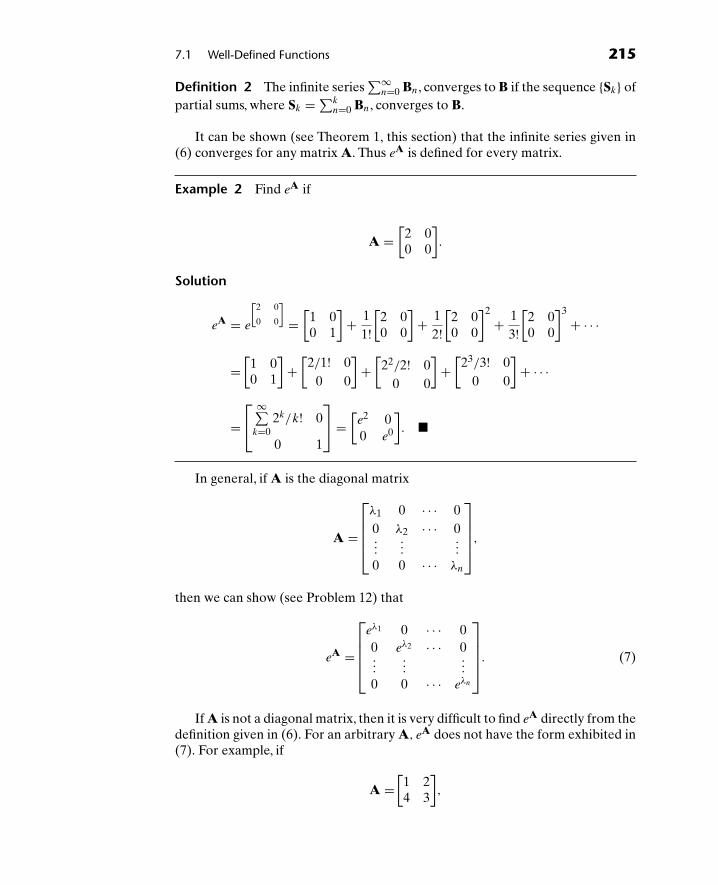
7.1 Well-Defined Functions 215
Definition 2 The infinite series∑∞
n=0 Bn, converges to B if the sequence {Sk} ofpartial sums, where Sk =∑k
n=0 Bn, converges to B.
It can be shown (see Theorem 1, this section) that the infinite series given in(6) converges for any matrix A. Thus eA is defined for every matrix.
Example 2 Find eA if
A =[
2 00 0
].
Solution
eA = e
[2 0
0 0
]=[
1 00 1
]+ 1
1![
2 00 0
]+ 1
2![
2 00 0
]2
+ 13![
2 00 0
]3
+ · · ·
=[
1 00 1
]+[
2/1! 00 0
]+[
22/2! 00 0
]+[
23/3! 00 0
]+ · · ·
=⎡⎣ ∞∑
k=02k/k! 0
0 1
⎤⎦ =
[e2 00 e0
]. �
In general, if A is the diagonal matrix
A =
⎡⎢⎢⎢⎣
λ1 0 · · · 00 λ2 · · · 0...
......
0 0 · · · λn
⎤⎥⎥⎥⎦,
then we can show (see Problem 12) that
eA =
⎡⎢⎢⎢⎣
eλ1 0 · · · 00 eλ2 · · · 0...
......
0 0 · · · eλn
⎤⎥⎥⎥⎦. (7)
If A is not a diagonal matrix, then it is very difficult to find eA directly from thedefinition given in (6). For an arbitrary A, eA does not have the form exhibited in(7). For example, if
A =[
1 24 3
],

216 Chapter 7 Matrix Calculus
it can be shown (however, not yet by us) that
eA = 16
[2e5 + 4e−1 2e5 − 2e−1
4e5 − 4e−1 4e5 + 2e−1
]
For the purposes of this book, the exponential is the only function that isneeded. However, it may be of some value to know how other functions of matrices,sines, cosines, etc., are defined. The following theorem, the proof of which is beyondthe scope of this book, provides this information.
Theorem 1 Let z represent the complex variable x + iy. If f(z) has the Taylorseries
∑∞k=0 akz
k, which converges for |z| < R, and if the eigenvalues λ1, λ2, . . . , λn
of an n × n matrix A have the property that |λi| < R(i = 1, 2, . . . , n), then∑∞k=0 akAk will converge to an n × n matrix which is defined to be f(A). In such a
case, f(A) is said to be well defined.
Example 3 Define sin A.
Solution A Taylor series for sin z is
sin z =∞∑
k=0
(−1)kz2k+1
(2k + 1)!
= z − z3
3! + z5
5! − z7
7! + · · · ·
This series can be shown to converge for all z (that is, R = ∞). Hence, sinceany eigenvalue λ of A must have the property |λ| < ∞ (that is, λ is finite) sin Acan be defined for every A as
sin A =∞∑
k=0
(−1)kA2k+1
(2k + 1)! = A − A3
3! + A5
5! − A7
7! + · · · · � (8)
Problems 7.1
1. Let q(x) = x − 1. Find pk(A) and q(A)pk(A) if
(a) A =⎡⎢⎣1 2 3
0 −1 40 0 1
⎤⎥⎦, k = 2, and p2(x) = x2 − 2x + 1,
(b) A =[
1 23 4
], k = 3, and p3(x) = 2x3 − 3x2 + 4.

7.1 Well-Defined Functions 217
2. If pk(x) is defined by (1), find pk(A) for the diagonal matrix
A =⎡⎢⎣λ1 0 0
0 λ2 00 0 λ3
⎤⎥⎦. Can you generalize?
3. By actually computing both sides of the following equation separately, verifythat (A − 3I)(A + 2I) = A2 − A − 6I for
(a) A =[
1 23 4
], (b) A =
⎡⎢⎣ 1 0 −2
3 1 1−2 −2 3
⎤⎥⎦.
The above equation is an example of matrix factoring.
4. Although x2 − y2 = (x − y)(x + y) whenever x and y denote real-valuedvariables, show by example that A2 − B2 need not equal the product(A − B)(A + B) whenever A and B denote 2 × 2 real matrices. Why?
5. It is known that x2 − 5x + 6 factors into the product (x − 2)(x − 3) wheneverx denotes a real-valued variable. Is it necessarily true that A2 − 5A + 6I =(A − 2I)(A − 3I) whenever A represents a square real matrix? Why?
6. Determine limk→∞ Bk when
Bk =⎡⎢⎣
1k
2 − 2k2
3 (0.5)k
⎤⎥⎦.
7. Determine limk→∞ Bk when
Bk =
⎡⎢⎢⎢⎢⎢⎢⎢⎢⎢⎢⎣
2k
k + 1
k + 3k2 − 2k + 1
3k2 + 2k
2k2
⎤⎥⎥⎥⎥⎥⎥⎥⎥⎥⎥⎦
.
8. Determine limk→∞ Dk when
Dk =[(0.2)k 1 (0.1)k
4 3k 0
].

218 Chapter 7 Matrix Calculus
9. It is known that arctan (z) =∑∞n=0[(−1)n/(2n + 1)]z2n+1 converges for all
|z| < π/2. Determine for which of the following matrices A, arctan(A) =∑∞n=0[(−1)n/2n + 1]A2n+1 is well defined:
(a)[−3 6−2 4
]. (b)
[5 −46 −5
]. (c)
[6 −52 −1
].
(d)
⎡⎣0 1 0
0 0 −10 1 0
⎤⎦. (e)
⎡⎣1 2 1
0 3 50 −1 −3
⎤⎦. (f)
⎡⎣0 1 0
0 0 1
0 − 18
34
⎤⎦.
10. It is known that ln(1 + z) =∑∞n=0[(−1)n+1/n]zn converges for all |z| < 1.
Determine for which of the matrices given in Problem 9 ln(I + A) =∑∞n=0[(−1)n+1/n]An is well defined.
11. It is known that f(z) =∑∞n=0 zn/3n converges for all |z| < 3. Determine for
which of the matrices given in Problem 9 f(A) =∑∞n=0 An/3n is well defined.
12. Derive Eq. (7).
13. Find eA when
A =[
1 00 2
].
14. Find eA when
A =[−1 0
0 28
].
15. Find eA when
A =⎡⎣2 0 0
0 −2 00 0 0
⎤⎦.
16. Derive an expression for sin(A) similar to Eq. (7) when A is a square diagonalmatrix.
17. Find sin(A) for the matrix given in Problem 13.
18. Find sin(A) for the matrix given in Problem 14.

7.2 Cayley–Hamilton Theorem 219
19. Using Theorem 1, give a definition for cos A and use this definition to find
cos[
1 00 2
].
20. Find cos(A) for the matrix given in Problem 15.
7.2 Cayley–Hamilton Theorem
We now state one of the most powerful theorems of matrix theory, the proof whichis given in the Final Comments at the end of this chapter.
Cayley–Hamilton Theorem. A matrix satisfies its own characteristic equation. Thatis, if the characteristic equation of an n × n matrix A is λn + an−1λ
n−1 + · · · + a1λ +a0 = 0, then
An + an−1An−1 + · · · + a1A + a0I = 0.
Note once again that when we change a scalar equation to a matrix equation,the unity element 1 is replaced by the identity matrix I.
Example 1 Verify the Cayley–Hamilton theorem for
A =[
1 24 3
].
Solution The characteristic equation for A is λ2 − 4λ − 5 = 0.
A2 − 4A − 5I =[
1 24 3
] [1 24 3
]− 4[
1 24 3
]− 5[
1 00 1
]
=[
9 816 17
]−[
4 816 12
]−[
5 00 5
]
=[
9 − 4 − 5 8 − 8 − 016 − 16 − 0 17 − 12 − 5
]=[
0 00 0
]= 0. �
Example 2 Verify the Cayley–Hamilton theorem for
A =⎡⎣3 0 −1
2 0 10 0 4
⎤⎦.

220 Chapter 7 Matrix Calculus
Solution The characteristic equation of A is (3 − λ)(−λ)(4 − λ) = 0.
(3I − A)(−A)(4I − A) =⎛⎝⎡⎣3 0 0
0 3 00 0 3
⎤⎦−
⎡⎣3 0 −1
2 0 10 0 4
⎤⎦⎞⎠⎛⎝−⎡⎣3 0 −1
2 0 10 0 4
⎤⎦⎞⎠
⎛⎝⎡⎣4 0 0
0 4 00 0 4
⎤⎦−
⎡⎣3 0 −1
2 0 10 0 4
⎤⎦⎞⎠
=⎡⎣ 0 0 1
−2 3 −10 0 −1
⎤⎦⎡⎣−3 0 1
−2 0 −10 0 −4
⎤⎦⎡⎣ 1 0 1
−2 4 −10 0 0
⎤⎦
=⎡⎣ 0 0 1
−2 3 −10 0 −1
⎤⎦⎡⎣−3 0 −3
−2 0 −20 0 0
⎤⎦ =
⎡⎣0 0 0
0 0 00 0 0
⎤⎦ = 0. �
One immediate consequence of the Cayley–Hamilton theorem is a newmethod for finding the inverse of a nonsingular matrix. If
λn + an−1λn−1 + · · · + a1λ + a0 = 0
is the characteristic equation of a matrix A, it follows from Problem 17 of Section6.4 that det(A) = (−1)na0. Thus, A is invertible if and only if a0 �= 0.
Now assume that a0 �= 0. By the Cayley–Hamilton theorem, we have
An + an−1An−1 + · · · + a1A + a0I = 0,
A[An−1 + an−1An−2 + · · · + a1I] = −a0I,
or
A[− 1
a0(An−1 + an−1An−2 + · · · + a1I)
]= I.
Thus, (−1/a0)(An−1 + an−1An−2 + · · · + a1I) is an inverse of A. But since theinverse is unique (see Theorem 2 of Section 3.4), we have that
A−1 = −1a0
(An−1 + an−1 An−2 + · · · + a1I). (9)
Example 3 Using the Cayley–Hamilton theorem, find A−1 for
A =⎡⎣1 −2 4
0 −1 22 0 3
⎤⎦.

7.2 Cayley–Hamilton Theorem 221
Solution The characteristic equation for A is λ3 − 3λ2 − 9λ + 3 = 0. Thus, bythe Cayley–Hamilton theorem,
A3 − 3A2 − 9A + 3I = 0.
Hence
A3 − 3A2 − 9A = −3I,
A(A2 − 3A − 9I) = −3I,
or,
A(
13
)(−A2 + 3A + 9I) = I.
Thus,
A−1 =(
13
)(−A2 + 3A + 9I
)
= 13
⎛⎝⎡⎣−9 0 −12
−4 −1 −4−8 4 −17
⎤⎦+
⎡⎣3 −6 12
0 −3 66 0 9
⎤⎦+
⎡⎣9 0 0
0 9 00 0 9
⎤⎦⎞⎠
= 13
⎡⎣ 3 −6 0
−4 5 2−2 4 1
⎤⎦. �
Problems 7.2
Verify the Cayley–Hamilton theorem and use it to find A−1, where possible, for:
1. A =[
1 23 4
], 2. A =
[1 22 4
],
3. A =⎡⎣2 0 1
4 0 20 0 −1
⎤⎦, 4. A =
⎡⎣1 −1 2
0 3 22 1 2
⎤⎦,
5. A =
⎡⎢⎢⎣
1 0 0 00 −1 0 00 0 −1 00 0 0 1
⎤⎥⎥⎦.

222 Chapter 7 Matrix Calculus
7.3 Polynomials of Matrices—Distinct Eigenvalues
In general, it is very difficult to compute functions of matrices from their definitionas infinite series (one exception is the diagonal matrix). The Cayley–Hamiltontheorem, however, provides a starting point for the development of an alternate,straightforward method for calculating these functions. In this section, we shalldevelop the method for polynomials of matrices having distinct eigenvalues. Inthe ensuing sections, we shall extend the method to functions of matrices havingarbitrary eigenvalues.
Let A represent an n × n matrix. Define d(λ) = det(A − λI). Thus, d(λ) isan nth degree polynomial in λ and the characteristic equation of A is d(λ) = 0.From Chapter 6, we know that if λi is an eigenvalue of A, then λi is a root of thecharacteristic equation, hence
d(λi) = 0. (10)
From the Cayley–Hamilton theorem, we know that a matrix must satisfy its owncharacteristic equation, hence
d(A) = 0. (11)
Let f(A) be any matrix polynomial of arbitrary degree that we wish to compute.f(λ) represents the corresponding polynomial of λ. A theorem of algebra statesthat there exist polynomials q(λ) and r(λ) such that
f(λ) = d(λ)q(λ) + r(λ), (12)
where r(λ) is called the remainder. The degree of r(λ) is less than that of d(λ),which is n, and must be less than or equal to the degree of f(λ) (why?).
Example 1 Find q(λ) and r(λ) if f(λ) = λ4 + 2λ3 − 1 and d(λ) = λ2 − 1.
Solution For λ �= ±1, d(λ) �= 0. Dividing f(λ) by d(λ), we obtain
f(λ)
d(λ)= λ4 + 2λ3 − 1
λ2 − 1=(λ2 + 2λ + 1
)+ 2λ
λ2 − 1,
f(λ)
d(λ)=(λ2 + 2λ + 1
)+ 2λ
d(λ),
or
f(λ) = d(λ)(λ2 + 2λ + 1
)(2λ). (13)
If we define q(λ) = λ2 + 2λ + 1 and r(λ) = 2λ, (13) has the exact form of (12) forall λ except possibly λ = ±1. However, by direct substitution, we find that (13) isalso valid for λ = ±1; hence (13) is an identity for all (λ). �
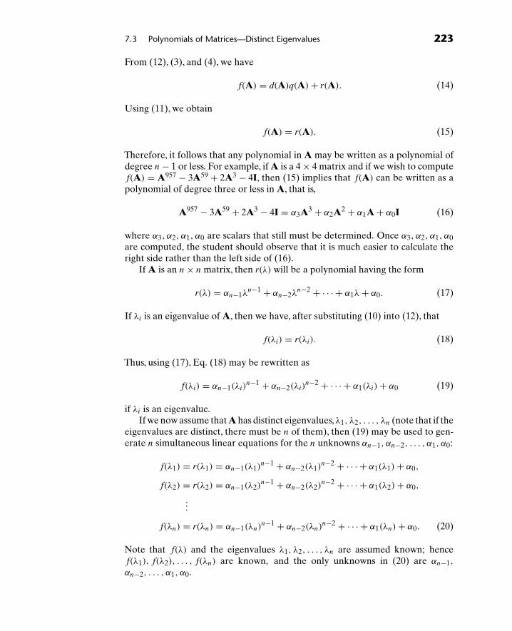
7.3 Polynomials of Matrices—Distinct Eigenvalues 223
From (12), (3), and (4), we have
f(A) = d(A)q(A) + r(A). (14)
Using (11), we obtain
f(A) = r(A). (15)
Therefore, it follows that any polynomial in A may be written as a polynomial ofdegree n − 1 or less. For example, if A is a 4 × 4 matrix and if we wish to computef(A) = A957 − 3A59 + 2A3 − 4I, then (15) implies that f(A) can be written as apolynomial of degree three or less in A, that is,
A957 − 3A59 + 2A3 − 4I = α3A3 + α2A2 + α1A + α0I (16)
where α3, α2, α1, α0 are scalars that still must be determined. Once α3, α2, α1, α0are computed, the student should observe that it is much easier to calculate theright side rather than the left side of (16).
If A is an n × n matrix, then r(λ) will be a polynomial having the form
r(λ) = αn−1λn−1 + αn−2λ
n−2 + · · · + α1λ + α0. (17)
If λi is an eigenvalue of A, then we have, after substituting (10) into (12), that
f(λi) = r(λi). (18)
Thus, using (17), Eq. (18) may be rewritten as
f(λi) = αn−1(λi)n−1 + αn−2(λi)
n−2 + · · · + α1(λi) + α0 (19)
if λi is an eigenvalue.If we now assume that A has distinct eigenvalues,λ1, λ2, . . . , λn (note that if the
eigenvalues are distinct, there must be n of them), then (19) may be used to gen-erate n simultaneous linear equations for the n unknowns αn−1, αn−2, . . . , α1, α0:
f(λ1) = r(λ1) = αn−1(λ1)n−1 + αn−2(λ1)
n−2 + · · · + α1(λ1) + α0,
f(λ2) = r(λ2) = αn−1(λ2)n−1 + αn−2(λ2)
n−2 + · · · + α1(λ2) + α0,
...
f(λn) = r(λn) = αn−1(λn)n−1 + αn−2(λn)
n−2 + · · · + α1(λn) + α0. (20)
Note that f(λ) and the eigenvalues λ1, λ2, . . . , λn are assumed known; hencef(λ1), f(λ2), . . . , f(λn) are known, and the only unknowns in (20) are αn−1,
αn−2, . . . , α1, α0.

224 Chapter 7 Matrix Calculus
Example 2 Find A593 if
A =[−3 −4
2 3
].
Solution The eigenvalues of A are λ1 = 1, λ2 = −1. For this example, f(A) =A593, thus, f(λ) = λ593. Since A is a 2 × 2 matrix, r(A) will be a polynomial ofdegree (2 − 1) = 1 or less, hence r(A) = α1A + α0I and r(λ) = α1λ + α0. From(15), we have that f(A) = r(A), thus, for this example,
A593 = α1A + α0I. (21)
From (18), we have that f(λi) = r(λi) if λi is an eigenvalue of A; thus, for thisexample, (λi)
593 = α1λi + α0. Substituting the eigenvalues of A into this equation,we obtain the following system for α1 and α0.
(1)593 = α1(1) + α0,
(−1)593 = α1(−1) + α0,
or
1 = α1 + α0,
−1 = −α1 + α0. (22)
Solving (22), we obtain α0 = 0, α1 = 1. Substituting these values into (21), weobtain A593 = 1 · A + 0 · I or
[−3 −42 3
]593
=[−3 −4
2 3
]. �
Example 3 Find A39 if
A =[
4 12 3
].
Solution The eigenvalues of A are λ1 = 5, λ2 = 2. For this example,f(A) = A39,thus f(λ) = λ39. Since A is a 2 × 2 matrix, r(A) will be a polynomial of degree 1or less, hence r(A) = α1A + α0I and r(λ) = α1λ + α0. From (15), we have thatf(A) = r(A), thus, for this example,
A39 = α1A + α0I. (23)

7.3 Polynomials of Matrices—Distinct Eigenvalues 225
From (18) we have that f(λi) = r(λi) if λi is an eigenvalue of A, thus for thisexample, (λi)
39 = α1λi + α0. Substituting the eigenvalues of A into this equation,we obtain the following system for α1 and α0:
539 = 5α1 + α0,
239 = 2α1 + α0. (24)
Solving (24), we obtain
α1 = 539 − 239
3, α0 = −2(5)39 + 5(2)39
3,
Substituting these values into (23), we obtain
A39 = 539 − 239
3
[4 12 3
]+ −2(5)39 + 5(2)39
3
[1 00 1
].
= 13
[2(5)39 + 239 539 − 239
2(5)39 − 2(2)39 539 + 2(2)39
]. (25)
The number 539 and 239 can be determined on a calculator. For our purposes,however, the form of (25) is sufficient and no further simplification is required. �
Example 4 Find A602 − 3A3 if
A =⎡⎣1 4 −2
0 0 00 −3 3
⎤⎦.
Solution The eigenvalues of A are λ1 = 0, λ2 = 1, λ3 = 3.
f(A) = A602 − 3A3, r(A) = α2A2 + α1A + α0I,
f(λ) = λ602 − 3λ3, r(λ) = α2λ2 + α1λ + α0.
Note that since A is a 3 × 3 matrix, r(A) must be no more than a second degreepolynomial. Now
f(A) = r(A);
thus,
A602 − 3A3 = α2A2 + α1A + α0I. (26)

226 Chapter 7 Matrix Calculus
If λi is an eigenvalue of A, then f(λi) = r(λi). Thus,
(λi)602 − 3(λi)
3 = α2(λi)2 + α1λi + α0;
hence,
(0)602 − 3(0)3 = α2(0)2 + α1(0) + α0,
(1)602 − 3(1)3 = α2(1)2 + α1(1) + α0,
(3)602 − 3(3)3 = α2(3)2 + α1(3) + α0,
or
0 = α0,
−2 = α2 + α1 + α0,
3602 − 81 = 9α2 + 3α1 + α0.
Thus,
α2 = 3602 − 756
, α1 = −(3)602 + 636
, α0 = 0. (27)
Substituting (27) into (26), we obtain
A602 − 3A3 = 3602 − 756
⎡⎣1 10 −8
0 0 00 −9 9
⎤⎦+ −(3)602 + 63
6
⎡⎣1 4 −2
0 0 00 −3 3
⎤⎦
= 16
⎡⎢⎣−12 6(3)602 − 498 −6(3)602 + 474
0 0 0
0 −6(3)602 + 486 6(3)602 − 486
⎤⎥⎦. �
Finally, the student should note that if the polynomial to be calculated is alreadyof a degree less than or equal to n − 1, then this method affords no simplificationand the polynomial must still be computed directly.
Problems 7.3
1. Specialize system (20) for f(A) = A7 and
A =[−2 3−1 2
].
Solve this system and use the results to determine A7. Check your answer bydirect calculations.

7.3 Polynomials of Matrices—Distinct Eigenvalues 227
2. Find A50 for the matrix A given in Problem 1.
3. Specialize system (20) for f(A) = A735 and
A =[
0 10 −1
].
Solve this system and use the results to determine A735 (What do you noticeabout A3?).
4. Specialize system (20) for f(A) = A20 and
A =[−3 6−1 2
].
Solve this system and use the results to determine A20.
5. Find A97 for the matrix A given in Problem 4.
6. Find A50 for the matrix A given in Example 3.
7. Specialize system (20) for f(A) = A78 and
A =[
2 −12 5
].
Solve this system and use the results to determine A78.
8. Find A41 for the matrix A given in Problem 7.
9. Specialize system (20) for f(A) = A222 and
A =⎡⎣1 −1 2
0 −1 20 0 2
⎤⎦.
Solve this system and use the results to determine A222.
10. Specialize system (20) for f(A) = A17, when A is a 3 × 3 matrix having 3, 5,and 10 as its eigenvalues.
11. Specialize system (20) for f(A) = A25, when A is a 4 × 4 matrix having2, −2, 3, and 4 as its eigenvalues.
12. Specialize system (20) for f(A) = A25, when A is a 4 × 4 matrix having1, −2, 3, and −4 as its eigenvalues.
13. Specialize system (20) for f(A) = A8, when A is a 5 × 5 matrix having1, −1, 2, −2, and 3 as its eigenvalues.
14. Specialize system (20) for f(A) = A8 − 3A5 + 5I, when A is the matrixdescribed in Problem 10.

228 Chapter 7 Matrix Calculus
15. Specialize system (20) for f(A) = A8 − 3A5 + 5I, when A is the matrixdescribed in Problem 11.
16. Specialize system (20) for f(A) = A8 − 3A5 + 5I, when A is the matrixdescribed in Problem 12.
17. Specialize system (20) for f(A) = A10 + 6A3 + 8A, when A is the matrixdescribed in Problem 12.
18. Specialize system (20) for f(A) = A10 + 6A3 + 8A, when A is the matrixdescribed in Problem 13.
19. Find A202 − 3A147 + 2I for the A of Problem 1.
20. Find A1025 − 4A5 for the A of Problem 1.
21. Find A8 − 3A5 − I for the matrix given in Problem 7.
22. Find A13 − 12A9 + 5I for
A =[
3 −51 −3
].
23. Find A10 − 2A5 + 10I for the matrix given in Problem 22.
24. Find A593 − 2A15 for
A =⎡⎣−2 4 3
0 0 0−1 5 2
⎤⎦.
25. Specialize system (20) for f(A) = A12 − 3A9 + 2A + 5I and
A =⎡⎣ 0 1 0
0 0 1−4 4 1
⎤⎦.
Solve this system, and use the results to determine f(A).
26. Specialize system (20) for f(A) = A9 − 3A4 + I and
A =⎡⎣ 0 1 0
0 0 1
− 116
14
14
⎤⎦.
Solve this system, and use the results to determine f(A).
7.4 Polynomials of Matrices—General Case
The only restriction in the previous section was that the eigenvalues of A hadto be distinct. The following theorem suggests how to obtain n equations for theunknown α’s in (15) even if some of the eigenvalues are identical.

7.4 Polynomials of Matrices—General Case 229
Theorem 1 Let f(λ) and r(λ) be defined as in Eq. (12). If λi is an eigenvalue ofmultiplicity k, then
f(λi) = r(λi),
df(λi)
dλ= dr(λi)
dλ,
d2f(λi)
dλ2 = d2r(λi)
dλ2 , (28)
...
dk−1f(λi)
dλk−1 = dk−1r(λi)
dλk−1 ,
where the notation dnf(λi)/dλn denotes the nth derivative of f(λ) with respect toλ evaluated at λ = λi.∗
Thus, for example, if λi is an eigenvalue of multiplicity 3, Theorem 1 impliesthat f(λ) and its first two derivatives evaluated at λ = λi are equal, respectively, tor(λ) and its first two derivatives also evaluated at λ = λi. If λi is an eigenvalue ofmultiplicity 5, then f(λ) and the first four derivatives of f(λ) evaluated at λ = λi areequal respectively to r(λ) and the first four derivatives of r(λ) evaluated at λ = λi.Note, furthermore, that if λi is an eigenvalue of multiplicity 1, then Theorem 1implies that f(λi) = r(λi), which is Eq. (18).
Example 1 Find A24 − 3A15 if
A =⎡⎣ 3 2 4
0 1 0−1 −3 −1
⎤⎦.
Solution The eigenvalues of A are λ1 = λ2 = λ3 = 1; hence, λ = 1 is aneigenvalue of multiplicity three.
f(A) = A24 − 3A15 r(A) = α2A2 + α1A + α0I
f(λ) = λ24 − 3λ15 r(λ) = α2λ2 + α1λ + α0
f ′(λ) = 24λ23 − 45λ14 r′(λ) = 2α2λ + α1
f ′′(λ) = 552λ22 − 630λ13 r′′(λ) = 2α2.
∗ Theorem 1 is proved by differentiating Eq. (12) k − 1 times and noting that if λi is an eigenvalue ofmultiplicity k, then
d(λi) = d[d(λi)]dλ
= · · · = d(k−1)d(λi)
dλk−1 = 0.

230 Chapter 7 Matrix Calculus
Now f(A) = r(A), hence
A24 − 3A15 = α2A2 + α1A + α0I. (29)
Also, since λ = 1 is an eigenvalue of multiplicity 3, it follows from Theorem 1 that
f(1) = r(1),
f ′(1) = r′(1),
f ′′(1) = r′′(1).
Hence,
(1)24 − 3(1)15 = α2(1)2 + α1(1) + α0,
24(1)23 − 45(1)14 = 2α2(1) + α1,
552(1)22 − 630(1)13 = 2α2,
or
−2 = α2 + α1 + α0,
−21 = 2α2 + α1,
−78 = 2α2.
Thus, α2 = −39, α1 = 57, α0 = −20, and from Eq. (29)
A24 − 3A15 = −39A2 + 57A − 20I =⎡⎣−44 270 −84
0 −2 021 −93 40
⎤⎦. �
Example 2 Set up the necessary equation to find A15 − 6A2 if
A =
⎡⎢⎢⎢⎢⎢⎢⎣
1 4 3 2 1 −70 0 2 11 1 00 0 1 −1 0 10 0 0 −1 2 10 0 0 0 −1 170 0 0 0 0 1
⎤⎥⎥⎥⎥⎥⎥⎦.
Solution The eigenvalues of A are λ1 = λ2 = λ3 = 1, λ4 = λ5 = −1, λ6 = 0.
f(A) = A15 − 6A2 r(A) = α5A5 + α4A4 + α3A3 + α2A2 + α1A + α0I
f(λ) = λ15 − 6λ2 r(λ) = α5λ5 + α4λ
4 + α3λ3 + α2λ
2 + α1λ1 + α0
f ′(λ) = 15λ14 − 12λ r′(λ) = 5α5λ4 + 4α4λ
3 + 3α3λ2 + 2α2λ + α1
f ′′(λ) = 210λ13 − 12 r′′(λ) = 20α5λ3 + 12α4λ
2 + 6α3λ + 2α2.

7.4 Polynomials of Matrices—General Case 231
Since f(A) = r(A),
A15 − 6A2 = a5A5 + α4A4 + α3A3 + α2A2 + α1A + α0I. (30)
Since λ = 1 is an eigenvalue of multiplicity 3, λ = −1 is an eigenvalue of multi-plicity 2 and λ = 0 is an eigenvalue of multiplicity 1, it follows from Theorem 1that
f(1) = r(1),
f ′(1) = r′(1),
f ′′(1) = r′′(1), (31)
f(−1) = r(−1),
f ′(−1) = r′(−1),
f(0) = r(0).
Hence,
(1)15 − 6(1)2 = α5(1)5 + α4(1)4 + α3(1)3 + α2(1)2 + α1(1) + α0
15(1)14 − 12(1) = 5α5(1)4 + 4α4(1)3 + 3α3(1)2 + 2α2(1) + α1
210(1)13 − 12 = 20α5(1)3 + 12α4(1)2 + 6α3(1) + 2α2
(−1)15 − 6(−1)2 = α5(−1)5 + α4(−1)4 + α3(−1)3 + α2(−1)2 + α1(−1) + α0
15(−1)14 − 12(−1) = 5α5(−1)4 + 4α4(−1)3 + 3α3(−1)2 + 2α2(−1) + α1
(0)15 − 12(0)2 = α5(0)5 + α4(0)4 + α3(0)3 + α2(0)2 + α1(0) + α0
or
−5 = α5 + α4 + α3 + α2 + α1 + α0
3 = 5α5 + 4α4 + 3α3 + 2α2 + α1
198 = 20α5 + 12α4 + 6α3 + 2α2 (32)
−7 = −α5 + α4 − α3 + α2 − α1 + α0
27 = 5α5 − 4α4 + 3α3 − 2α2 + α1
0 = α0.
System (32) can now be solved uniquely for α5, α4, . . . , α0; the results are thensubstituted into (30) to obtain f(A). �

232 Chapter 7 Matrix Calculus
Problems 7.4
1. Using Theorem 1, establish the equations that are needed to find A7 if A is a2 × 2 matrix having 2 and 2 as multiple eigenvalues.
2. Using Theorem 1, establish the equations that are needed to find A7 if A is a3 × 3 matrix having 2 as an eigenvalue of multiplicity three.
3. Redo Problem 2 if instead the eigenvalues are 2, 2, and 1.
4. Using Theorem 1, establish the equations that are needed to find A10 if A isa 2 × 2 matrix having 3 as an eigenvalue of multiplicity two.
5. Redo Problem 4 if instead the matrix has order 3 × 3 with 3 as an eigenvalueof multiplicity three.
6. Redo Problem 4 if instead the matrix has order 4 × 4 with 3 as an eigenvalueof multiplicity four.
7. Using Theorem 1, establish the equations that are needed to find A9 if A is a4 × 4 matrix having 2 as an eigenvalue of multiplicity four.
8. Redo Problem 7 if instead the eigenvalues are 2, 2, 2, and 1.
9. Redo Problem 7 if instead the eigenvalues are 2 and 1, both with multiplicitytwo.
10. Set up (but do not solve) the necessary equations to find A10 − 3A5 if
A =
⎡⎢⎢⎢⎢⎢⎢⎣
5 −2 1 1 5 −70 5 2 1 −1 10 0 5 0 1 −30 0 0 2 1 20 0 0 0 2 00 0 0 0 0 5
⎤⎥⎥⎥⎥⎥⎥⎦.
11. Find A6 in two different ways if
A =[
5 8−2 −5
].
(First find A6 using Theorem 1, and then by direct multiplication.)
12. Find A521 if
A =⎡⎣4 1 −3
0 −1 05 1 −4
⎤⎦.

7.5 Functions of a Matrix 233
13. Find A14 − 3A13 if
A =⎡⎣ 4 1 2
0 0 0−8 1 −4
⎤⎦.
7.5 Functions of a Matrix
Once the student understands how to compute polynomials of a matrix, com-puting exponentials and other functions of a matrix is easy, because the methodsdeveloped in the previous two sections remain valid for more general functions.
Let f(λ) represent a function of λ and suppose we wish to compute f(A). Itcan be shown, for a large class of problems, that there exists a function q(λ) andan n − 1 degree polynomial r(λ) (we assume A is of order n × n) such that
f(λ) = q(λ)d(λ) + r(λ), (33)
where d(λ) = det(A − λI). Hence, it follows that
f(A) = q(A)d(A) + r(A). (34)
Since (33) and (34) are exactly Eqs. (12) and (14), where f(λ) is now understoodto be a general function and not restricted to polynomials, the analysis of Sections7.3 and 7.4 can again be applied. It then follows that
(a) f(A) = r(A), and(b) Theorem 1 of Section 7.4 remains valid
Thus, the methods used to compute a polynomial of a matrix can be generalizedand used to compute arbitrary functions of a matrix.
Example 1 Find eA if
A =[
1 24 3
].
Solution The eigenvalues of A are λ1 = 5, λ2 = −1; thus,
f(A) = eA r(A) = α1A + α0I
f(λ) = eλ r(λ) = α1λ + α0.
Now f(A) = r(A); hence
eA = α1A + α0I. (35)

234 Chapter 7 Matrix Calculus
Also, since Theorem 1 of Section 7.4 is still valid,
f(5) = r(5),
and
f(−1) = r(−1);
hence,
e5 = 5α1 + α0,
e−1 = −α1 + α0.
Thus,
α1 = e5 − e−1
6and α0 = e5 + 5e−1
6.
Substituting these values into (35), we obtain
eA = 16
[2e5 + 4e−1 2e5 − 2e−1
4e5 − 4e−1 4e5 + 2e−1
]. �
Example 2 Find eA if
A =⎡⎣2 1 0
0 2 10 0 2
⎤⎦.
Solution The eigenvalues of A are λ1 = λ2 = λ3 = 2, thus,
f(A) = eA r(A) = α2A2 + α1A + α0If(λ) = eλ r(λ) = α2λ
2 + α1λ + α0
f ′(λ) = eλ r′(λ) = 2α2λ + α1
f ′′(λ) = eλ r′′(λ) = 2α2.
since f(A) = r(A),
eA = α2A2 + α1A + α0I. (36)

7.5 Functions of a Matrix 235
Since λ = 2 is an eigenvalue of multiplicity three,
f(2) = r(2),
f ′(2) = r′(2),
f ′′(2) = r′′(2);
hence,
e2 = 4α2 + 2α1 + α0,
e2 = 4α2 + α1,
e2 = 2α2,
or
α2 = e2
2, α1 = −e2, α0 = e2.
Substituting these values into (36), we obtain
eA = e2
2
⎡⎣4 4 1
0 4 40 0 4
⎤⎦− e2
⎡⎣2 1 0
0 2 10 0 2
⎤⎦+ e2
⎡⎣1 0 0
0 1 00 0 1
⎤⎦ =
⎡⎣e2 e2 e2/2
0 e2 e2
0 0 e2
⎤⎦. �
Example 3 Find sin A if
A =⎡⎣π 1 0
0 π 04 1 π/2
⎤⎦.
Solution The eigenvalues of A are λ1 = π/2, λ2 = λ3 = π; thus
f(A) = sin A r(A) = α2A2 + α1A + α0I
f(λ) = sin λ r(λ) = α2λ2 + α1λ + α0
f ′(λ) = cos λ r′(λ) = 2α2λ + α1.
But f(A) = r(A), hence
sin A = α2A2 + α1A + α0I. (37)

236 Chapter 7 Matrix Calculus
Since λ = π/2 is an eigenvalue of multiplicity 1 and λ = π is an eigenvalue ofmultiplicity 2, it follows that
f(π/2) = r(π/2),
f(π) = r(π),
f ′(π) = r′(π);hence,
sin π/2 = α2(π/2)2 + α1(π/2) + α0,
sin π = α2(π)2 + α1(π) + α0,
cos π = 2α2π + α1,
or simplifying
4 = α2π2 + 2α1π + 4α0,
0 = α2π2 + α1π + α0,
−1 = 2α2π + α1.
Thus, α2 = (1/π2)(4 − 2π), α1 = (1/π2)(−8π + 3π2), α0 = (1/π2)(4π2 − π3). Sub-stituting these values into (37), we obtain
sin A = 1/π2
⎡⎣ 0 −π2 0
0 0 0−8π 16 − 10π π2
⎤⎦. �
In closing, we point out that although exponentials of any square matrix canalways be computed by the above methods, not all functions of all matrices can;f(A) must first be “well defined” whereby “well defined” (see Theorem 1 of Sec-tion 7.1) we mean that f(z) has a Taylor series which converges for |z| < R andall eigenvalues of A have the property that their absolute values are also lessthan R.
Problems 7.5
1. Establish the equations necessary to find eA if A is a 2 × 2 matrix having 1 and2 as its eigenvalues.
2. Establish the equations necessary to find eA if A is a 2 × 2 matrix having 2 and2 as multiple eigenvalues.
3. Establish the equations necessary to find eA if A is a 3 × 3 matrix having 2 asan eigenvalue of multiplicity three.

7.5 Functions of a Matrix 237
4. Establish the equations necessary to find eA if A is a 3 × 3 matrix having 1,−2, and 3 as its eigenvalues.
5. Redo Problem 4 if instead the eigenvalues are −2, −2, and 1.
6. Establish the equations necessary to find sin(A) if A is a 3 × 3 matrix having1, 2, and 3 as its eigenvalues.
7. Redo Problem 6 if instead the eigenvalues are −2, −2, and 1.
8. Establish the equations necessary to find eA if A is a 4 × 4 matrix having 2 asan eigenvalue of multiplicity four.
9. Establish the equations necessary to find eA if A is a 4 × 4 matrix having both2 and −2 as eigenvalues of multiplicity two.
10. Redo Problem 9 if instead the function of interest is sin(A).
11. Establish the equations necessary to find eA if A is a 4 × 4 matrix having 3, 3,3, and −1 as its eigenvalues.
12. Redo Problem 11 if instead the function of interest is cos(A).
13. Find eA for
A =[
1 34 2
].
14. Find eA for
A =[
4 −11 2
].
15. Find eA for
A =⎡⎣ 1 1 2
−1 3 40 0 2
⎤⎦.
16. Find eA for
A =⎡⎣1 1 2
3 −1 40 0 2
⎤⎦.
17. Find cos A if
A =[
π 3π
2π 2π
].

238 Chapter 7 Matrix Calculus
18. The function f(z) = log(1 + z) has the Taylor series
∞∑k=1
(−1)k−1zk
k
which converges for |z| < 1. For the following matrices, A, determine whetheror not log(A + I) is well defined and, if so, find it.
(a)
[12 1
0 − 12
](b)
[−6 9−2 3
](c)[
3 5−1 −3
](d)
[0 00 0
].
7.6 The Function eAt
A very important function in the matrix calculus is eAt , where A is a square constantmatrix (that is, all of its entries are constants) and t is a variable. This function maybe calculated by defining a new matrix B = At and then computing eB by themethods of the previous section.
Example 1 Find eAt if
A =[
1 24 3
].
Solution Define
B = At =[
t 2t
4t 3t
].
The problem then reduces to finding eB. The eigenvalues of B are λ1 = 5t, λ2 = −t.Note that the eigenvalues now depend on t.
f(B) = eB r(B) = α1B + α0If(λ) = eλ r(λ) = α1λ + α0.
Since f(B) = r(B),
eB = α1B + α0I. (38)
Also, f(λi) = r(λi); hence
e5t = α1(5t) + α0,
e−t = α1(−t) + α0.

7.6 The Function eAt 239
Thus, α1 = (1/6t)(e5t − e−t) and α0 = (1/6)(e5t + 5e−t). Substituting these valuesinto (38), we obtain
eAt = eB =(
16t
)(e5t − e−t
) [t 2t
4t 3t
]+(
16
)(e5t + 5e−t
) [1 00 1
]
= 16
[2e5t + 4e−t 2e5t − 2e−t
4e5t − 4e−t 4e5t + 2e−t
]. �
Example 2 Find eAt if
A =⎡⎣3 1 0
0 3 10 0 3
⎤⎦.
Solution Define
B = At =⎡⎣3t t 0
0 3t t
0 0 3t
⎤⎦.
The problem reduces to finding eB. The eigenvalues of B are
λ1 = λ2 = λ3 = 3t
thus,
f(B) = eB r(B) = α2B2 + α1B + α0I
f(λ) = eλ r(λ) = α2λ2 + α1λ + α0
(39)
f ′(λ) = eλ r′(λ) = 2α2λ + α1 (40)
f ′′(λ) = eλ r′′(λ) = 2α2. (41)
Since f(B) = r(B),
eB = α2B2 + α1B + α0I. (42)
Since λ = 3t is an eigenvalue of multiplicity 3,
f(3t) = r(3t), (43)
f ′(3t) = r′(3t), (44)
f ′′(3t) = r′′(3t). (45)

240 Chapter 7 Matrix Calculus
Thus, using (39)–(41), we obtain
e3t = (3t)2α2 + (3t)α1 + α0,
e3t = 2(3t)α2 + α1,
e3t = 2α2
or
e3t = 9t2α2 + 3tα1 + α0, (46)
e3t = 6tα2 + α1, (47)
e3t = 2α2. (48)
Solving (46)–(48) simultaneously, we obtain
α2 = 12e3t , α1 = (1 − 3t)e3t , α0 = (1 − 3t + 9
2 t2)e3t .
From (42), it follows that
eAt = eB = 12e3t
⎡⎣9t2 6t2 t2
0 9t2 6t2
0 0 9t2
⎤⎦+ (1 − 3t)e3t
⎡⎣3t t 0
0 3t t
0 0 3t
⎤⎦
+ (1 − 3t + 92 t2)e3t
⎡⎣1 0 0
0 1 00 0 1
⎤⎦
= e3t
⎡⎣1 t t2/2
0 1 t
0 0 1
⎤⎦. �
Problems 7.6
Find eAt if A is given by:
1.[
4 43 5
]. 2.
[2 1
−1 −2
]. 3.
[4 1
−1 2
].
4.[
0 1−14 −9
]. 5.
[−3 22 −6
]. 6.
[−10 66 −10
].
7.
⎡⎣0 1 0
0 0 10 0 0
⎤⎦. 8.
⎡⎣ 1 0 0
4 1 2−1 4 −1
⎤⎦.

7.7 Complex Eigenvalues 241
7.7 Complex Eigenvalues
When computing eAt , it is often the case that the eigenvalues of B = At arecomplex. If this occurs the complex eigenvalues will appear in conjugate pairs,assuming the elements of A to be real, and these can be combined to produce realfunctions.
Let z represent a complex variable. Define ez by
ez =∞∑
k=0
zk
k! = 1 + z + z2
2! + z3
3! + z4
4! + z5
5! + · · · (49)
(see Eq. (5)). Setting z = iθ, θ real, we obtain
eiθ = 1 + iθ + (iθ)2
2! + (iθ)3
3! + (iθ)4
4! + (iθ)5
5! + · · ·
= 1 + iθ − θ2
2! − iθ3
3! + θ4
4! + iθ5
5! − · · · ·
Combining real and imaginary terms, we obtain
eiθ =(
1 − θ2
2! + θ4
4! − · · ·)
+ i
(θ − θ3
3! + θ5
5! − · · ·)
. (50)
But the Maclaurin series expansions for sin θ and cos θ are
sin θ = θ
1! − θ3
3! + θ5
5! − · · ·
cos θ = 1 − θ2
2! + θ4
4! + θ6
6! + · · · ;
hence, Eq. (50) may be rewritten as
eiθ = cos θ + i sin θ. (51)
Equation (51) is referred to as DeMoivre’s formula. If the same analysis is appliedto z = −iθ, it follows that
e−iθ = cos θ − i sin θ. (52)
Adding (51) and (52), we obtain
cos θ = eiθ + e−iθ
2, (53)

242 Chapter 7 Matrix Calculus
while subtracting (52) from (51), we obtain
sin θ = eiθ − e−iθ
2i. (54)
Equations (53) and (54) are Euler’s relations and can be used to reducecomplex exponentials to expressions involving real numbers.
Example 1 Find eAt if
A =[−1 5−2 1
].
Solution
B = At =[ −t 5t
−2t t
].
Hence the eigenvalues of B are λ1 = 3ti and λ2 = −3ti; thus
f(B) = eB r(B) = α1B + α0I
f(λ) = eλ r(λ) = α1λ + α0
Since f(B) = r(B),
eB = α1B + α0I, (55)
and since f(λi) = r(λi),
e3ti = α1(3ti) + α0,
e−3ti = α1(−3ti) + α0.
Thus,
α0 = e3ti + e−3ti
2and α1 = 1
3t
(e3ti − e−3ti
2i
).
If we now use (53) and (54), where in this case θ = 3t, it follows that
α0 = cos 3t and α1 = (1/3t) sin 3t.
Substituting these values into (55), we obtain
eAt = eB =[− 1
3 sin 3t + cos 3t 53 sin 3t
− 23 sin 3t 1
3 sin 3t + cos 3t
]. �

7.7 Complex Eigenvalues 243
In Example 1, the eigenvalues of B are pure imaginary permitting theapplication of (53) and (54) in a straightforward manner. In the general case,where the eigenvalues are complex numbers, we can still use Euler’s relationsproviding we note the following:
eβ+iθ + eβ−iθ
2= eβeiθ + eβe−iθ
2= eβ
(eiθ + e−iθ
)2
= eβ cos θ, (56)
and
eβ+iθ − eβ−iθ
2i= eβeiθ − eβe−iθ
2i= eβ
(eiθ − e−iθ
)2i
= eβ sin θ. (57)
Example 2 Find eAt if
A =[
2 −14 1
].
Solution
B = At =[
2t −t
4t t
];
hence, the eigenvalues of B are
λ1 =(
32
+ i
√152
)t, λ2 =
(32
− i
√152
)t.
Thus,
f(B) = eB r(B) = α1B + α0I
f(λ) = eλ r(λ) = α1λ + α0.
Since f(B) = r(B),
eB = α1B + α0I, (58)
and since f(λi) = r(λi),
e[3/2+i(√
15/2)]t = α1[ 32 + i(
√15/2)]t + α0,
e[3/2−i(√
15/2)]t = α1[ 32 − i(
√15/2)]t + α0.

244 Chapter 7 Matrix Calculus
Putting this system into matrix form, and solving for α1 and α0 by inversion, weobtain
α1 = 2√15t
[e[(3/2)t+(
√15/2)ti] − e[(3/2)t−(
√15/2)ti]
2i
]
α0 = −3√15
(e[(3/2)t+(
√15/2)ti] − e[(3/2)t−(
√15/2)ti]
2i
)
+(
e[(3/2)t+(√
15/2)ti] + e[(3/2)t−(√
15/2)ti]
2
).
Using (56) and (57) where, β = 32 t and θ = (
√15/2)t, we obtain
α1 = 2√15t
e3t/2 sin
√15t
2
α0 = − 3√15
e3t/2 sin
√152
t + e3t/2 cos
√152
t.
Substituting these values into (58), we obtain
eAt = e3t/2
⎡⎢⎢⎢⎢⎣
1√15
sin
√152
t + cos
√152
t−2√
15sin
√152
t
8√15
sin
√152
t−1√
15sin
√152
t + cos
√152
t
⎤⎥⎥⎥⎥⎦. �
Problems 7.7
Find eAt if A is given by:
1.[
1 −15 −1
]. 2.
[2 −23 −2
]. 3.
[0 1
−64 0
].
4.[
4 −810 −4
]. 5.
[2 5
−1 −2
]. 6.
[0 1
−25 −8
].
7.[
3 1−2 5
]. 8.
⎡⎣0 1 0
0 −2 −50 1 2
⎤⎦.

7.8 Properties of eA 245
7.8 Properties of eA
Since the scalar function ex and the matrix function eA are defined similarly (seeEqs. (5) and (6)), it should not be surprising to find that they possess some similarproperties. What might be surprising, however, is that not all properties of ex arecommon to eA. For example, while it is always true that exey = ex+y = eyex, thesame cannot be said for matrices eA and eB unless A and B commute.
Example 1 Find eAeB, eA+B, and eBeA if
A =[
1 10 0
]and B =
[0 00 1
].
Solution Using the methods developed in Section 7.5, we find
eA =[e e − 10 1
], eB =
[1 00 e
], eA+B =
[e e
0 e
].
Therefore,
eAeB =[e e − 10 1
] [1 00 e
]=[e e2 − e
0 e
]
and
eBeA =[
1 00 e
] [e e − 10 1
]=[e e − 10 e
];
hence
eA+B �= eAeB, eA+B �= eBeA and eBeA �= eAeB. �
Two properties that both ex and eA do have in common are given by thefollowing:
Property 1 e0 = I, where 0 represents the zero matrix.
Proof. From (6) we have that
eA =∞∑
k=0
(Ak
k!)
= I +∞∑
k=1
(Ak
k!)
.
Hence,
e0 = I +∞∑
k=1
0k
k! = I.

246 Chapter 7 Matrix Calculus
Property 2 (eA)−1 = e−A.
Proof.
(eA)(e−A) =[ ∞∑
k=0
(Ak
k!)][ ∞∑
k=0
(−A)k
k!
]
=[
I + A + A2
2! + A3
3! + · · ·][
I − A + A2
2! − A3
3! + · · ·]
= II + A [1 − 1] + A2[
12 ! − 1 + 1
2 !]
+ A3[− 1
3 ! + 12 ! − 1
2 ! + 13 !]
+ · · ·= I.
Thus, e−A is an inverse of eA. However, by definition, an inverse of eA is (eA)−1;hence, from the uniqueness of the inverse (Theorem 2 of Section 3.4), we havethat e−A = (eA)−1.
Example 2 Verify Property 2 for
A =[
0 10 0
].
Solution
−A =[
0 −10 0
],
eA =[
1 10 1
], and e−A =
[1 −10 1
].
Thus,
(eA)−1 =[
1 10 1
]−1
=[
1 −10 1
]= e−A. �
Note that Property 2 implies that eA is always invertible even if A itself is not.
Property 3 (eA)T = eAT.
Proof. The proof of this property is left as an exercise for the reader (seeProblem 7).

7.8 Properties of eA 247
Example 3 Verify Property 3 for
A =[
1 24 3
].
Solution
AT =[
1 42 3
],
eAT = 16
[2e5 + 4e−1 4e5 − 4e−1
2e5 − 2e−1 4e5 + 2e−1
].
and
eA = 16
[2e5 + 4e−1 2e5 − 2e−1
4e5 − 4e−1 4e5 + 2e−1
];
Hence, (eA)T = eAT. �
Problems 7.8
1. Verify Property 2 for
A =[
1 30 1
].
2. Verify Property 2 for
A =[
0 1−64 0
].
3. Verify Property 2 for
A =⎡⎣0 1 0
0 0 10 0 0
⎤⎦.
What is the inverse of A?
4. Verify Property 3 for
A =⎡⎣2 1 0
0 2 01 −1 1
⎤⎦.

248 Chapter 7 Matrix Calculus
5. Verify Property 3 for the matrix given in Problem 2.
6. Verify Property 3 for the matrix given in Problem 3.
7. Prove Property 3. (Hint: Using the fact that the eigenvalues of A are identicalto eigenvalues of AT, show that if eA = αn−1An−1 + · · · + α1A + α0I, and if
eAT = βn−1(AT)n−1 + · · · + β1AT + β0I,
then αj = βj for j = 0, 1, . . . , n − 1.)
8. Find eAeB, eBeA, and eA+B if
A =[
1 10 0
]and B =
[0 10 1
]
and show that eA+B �= eAeB, eA+B �= eBeA and eBeA �= eAeB.
9. Find two matrices A and B such that
eAeB = eA+B.
10. By using the definition of eA, prove that if A and B commute, then eAeB =eA+B.
11. Show that if A = P−1BP for some invertible matrix P, then eA = P−1eBP.
7.9 Derivatives of a Matrix
Definition 1 An n × n matrix A(t) = [aij(t)] is continuous at t = t0 if each of itselements aij(t)(i, j = 1, 2, . . . , n) is continuous at t = t0.
For example, the matrix given in (59) is continuous everywhere because eachof its elements is continuous everywhere while the matrix given in (60) is notcontinuous at t = 0 because the (1, 2) element, sin(1/t), is not continuous at t = 0.
[et t2 − 1
2 sin2 t
](59)
[t3 − 3t sin(1/t)
2t 45
](60)
We shall use the notation A(t) to emphasize that the matrix A may depend onthe variable t.

7.9 Derivatives of a Matrix 249
Definition 2 An n × n matrix A(t) = [aij(t)] is differentiable at t = t0 if each ofthe elements aij(t)(i, j = 1, 2, . . . , n) is differentiable at t = t0 and
dA(t)
dt=[daij(t)
dt
]. (61)
Generally we will use the notation A(t) to represent dA(t)/dt.
Example 1 Find A(t) if
A(t) =[
t2 sin t
ln t et2
].
Solution
A(t) = dA(t)
dt=
⎡⎢⎢⎢⎣
d(t2)
dt
d(sin t)
dt
d(ln t)
dt
d(et2)
dt
⎤⎥⎥⎥⎦ =
[2t cos t
1t
2tet2
]. �
Example 2 Find A(t) if
A(t) =⎡⎢⎣3t
45t2
⎤⎥⎦.
Solution
A(t) =
⎡⎢⎢⎢⎢⎢⎢⎣
d(3t)
dtd(45)
dt
d(t2)
dt
⎤⎥⎥⎥⎥⎥⎥⎦ =
⎡⎣ 3
02t
⎤⎦. �
Example 3 Find x(t) if
x(t) =
⎡⎢⎢⎣
x1(t)
x2(t)...
xn(t)
⎤⎥⎥⎦.
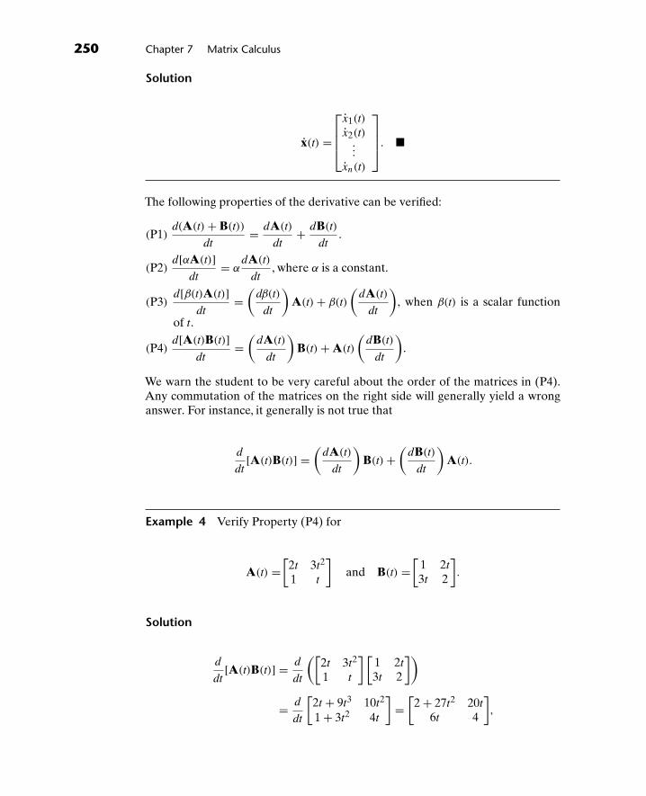
250 Chapter 7 Matrix Calculus
Solution
x(t) =
⎡⎢⎢⎣
x1(t)
x2(t)...
xn(t)
⎤⎥⎥⎦. �
The following properties of the derivative can be verified:
(P1)d(A(t) + B(t))
dt= dA(t)
dt+ dB(t)
dt.
(P2)d[αA(t)]
dt= α
dA(t)
dt, where α is a constant.
(P3)d[β(t)A(t)]
dt=(
dβ(t)
dt
)A(t) + β(t)
(dA(t)
dt
), when β(t) is a scalar function
of t.
(P4)d[A(t)B(t)]
dt=(
dA(t)
dt
)B(t) + A(t)
(dB(t)
dt
).
We warn the student to be very careful about the order of the matrices in (P4).Any commutation of the matrices on the right side will generally yield a wronganswer. For instance, it generally is not true that
d
dt[A(t)B(t)] =
(dA(t)
dt
)B(t) +
(dB(t)
dt
)A(t).
Example 4 Verify Property (P4) for
A(t) =[
2t 3t2
1 t
]and B(t) =
[1 2t
3t 2
].
Solution
d
dt[A(t)B(t)] = d
dt
([2t 3t2
1 t
] [1 2t
3t 2
])
= d
dt
[2t + 9t3 10t2
1 + 3t2 4t
]=[
2 + 27t2 20t
6t 4
],

7.9 Derivatives of a Matrix 251
and [dA(t)
dt
]B(t) + A(t)
[dB(t)
dt
]=[
2 6t
0 1
] [1 2t
3t 2
]+[
2t 3t2
1 t
] [0 23 0
]
=[
2 + 27t2 20t
6t 4
]
= d[A(t)B(t)]dt
. �
We are now in a position to establish one of the more important properties ofeAt . It is this property that makes the exponential so useful in differential equations(as we shall see in Chapter 8) and hence so fundamental in analysis.
Theorem 1 If A is a constant matrix then
deAt
dt= AeAt = eAtA.
Proof. From (6) we have that
eAt =∞∑
k=0
(At)k
k!
or
eAt = I + tA + t2A2
2! + t3A3
3! + · · · + tn−1An−1
(n − 1)! + tnAn
n! + tn+1An+1
(n + 1)! + · · ·
Therefore,
deAt
dt= 0 + A
1! + 2tA2
2! + 3t2A3
3! + · · · + ntn−1An
n! + (n + 1)tnAn+1
(n + 1)! + · · ·
= A + tA2
1! + t2A3
2! + · · · + tn−1An
(n − 1)! + tnAn+1
n! + · · ·
=[
I + tA1! + t2A2
2! + · · · + tn−1An−1
(n − 1)! + tnAn
n! + · · ·]
A
= eAtA.
If we had factored A on the left, instead of on the right, we would have obtainedthe other identity,
deAt
dt= AeAt .

252 Chapter 7 Matrix Calculus
Corollary 1 If A is a constant matrix, then
de−At
dt= −Ae−At = −e−AtA.
Proof. Define C = −A. Hence, e−At = eCt . Since C is a constant matrix, usingTheorem 1, we have
deCt
dt= CeCt = eCtC.
If we now substitute for C its value, −A, Corollary 1 is immediate.
Definition 3 An n × n matrix A(t) = [aij(t)] is integrable if each of its elementsaij(t)(i, 1, 2, . . . , n) is integrable, and if this is the case,
∫A(t) dt =
[∫aij(t) dt
].
Example 5 Find∫
A(t) dt if
A(t) =[
3t 2t2 et
].
Solution
∫A(t) dt =
[∫3t dt
∫2 dt∫
t2 dt∫
et dt
]=⎡⎣(
32
)t2 + c1 2t + c2(
13
)t3 + c3 et + c4
⎤⎦. �
Example 6 Find∫ 1
0 A(t) dt if
A(t) =⎡⎣ 2t 1 2
et 6t2 −1sin πt 0 1
⎤⎦.

7.9 Derivatives of a Matrix 253
Solution
∫ 1
0A(t) dt =
⎡⎢⎢⎢⎢⎢⎢⎢⎣
∫ 1
02t dt
∫ 1
01 dt
∫ 1
02 dt∫ 1
0et dt
∫ 1
06t2 dt
∫ 1
0−1 dt∫ 1
0sin πt dt
∫ 1
00 dt
∫ 1
01 dt
⎤⎥⎥⎥⎥⎥⎥⎥⎦
=⎡⎣ 1 1 2
e − 1 2 −12/π 0 1
⎤⎦. �
The following property of the integral can be verified:
(P5)
∫[αA(t) + βB(t)] dt = α
∫A(t) dt + β
∫B(t) dt,
where α and β are constants.
Problems 7.9
1. Find A(t) if
(a) A(t) =[
cos t t2 − 12t e(t−1)
].
(b) A(t) =⎡⎣ 2et3 t(t − 1) 17
t2 + 3t − 1 sin 2t t
cos3(3t2) 4 ln t
⎤⎦.
2. Verify Properties (P1) – (P4) for
α = 7, β(t) = t2, A(t) =[t3 3t2
1 2t
], and B(t) =
[t −2t
t3 t5
].
3. Prove that if dA(t)/dt = 0, then A(t) is a constant matrix. (That is, a matrixindependent of t).
4. Find∫
A(t) dt for the A(t) given in Problem 1(a).
5. Verify Property (P5) for
α = 2, β = 10, A(t) =[
6t t2
2t 1
], and B(t) =
[t 4t2
1 2t
].

254 Chapter 7 Matrix Calculus
6. Using Property (P4), derive a formula for differentiating A2(t). Use thisformula to find dA2(t)/dt, where
A(t) =[
t 2t2
4t3 et
],
and, show that dA2(t)/dt �= 2A(t) dA(t)/dt. Therefore, the power rule of dif-ferentiation does not hold for matrices unless a matrix commutes with itsderivative.
7.10 Final Comments on Chapter 7
We begin a proof of the Cayley–Hamilton theorem by noting that if B is an n × n
matrix having elements which are polynomials in λ with constant coefficients,then B can be expressed as a matrix polynomial in λ whose coefficients are n × n
constant matrices. As an example, consider the following decomposition:
[λ3 + 2λ2 + 3λ + 4 2λ3 + 3λ2 + 4λ + 5
3λ3 + 4λ2 + 5λ 2λ + 3
]
=[
1 23 0
]λ3 +
[2 34 0
]λ2 +
[3 45 2
]λ +
[4 50 3
].
In general, if the elements of B are polynomials of degree k or less, then
B = Bkλk + Bk−1λ
k−1 + · · · + B1λ + B0,
where Bj (j = 0, 1, . . . , k) is an n × n constant matrix.Now let A be any arbitrary n × n matrix. Define
C =(A − λI) (62)
and let
d(λ) = λn + an−1λn−1 + · · · + a1λ + a0 (63)
represent the characteristic polynomial of A. Thus,
d(λ) = det(A − λI) = det C. (64)
Since C is an n × n matrix, it follows that the elements of Ca (see Definition 2 ofSection 5.5) will be polynomials in λ of either degree n − 1 or n − 2. (Elements

7.10 Final Comments 255
on the diagonal of Ca will be polynomials of degree n − 1 while all other elementswill be polynomials of degree n − 2.) Thus, Ca can be written as
Ca = Cn−1λn−1 + Cn−2λ
n−2 + · · · + C1λ + C0, (65)
where Cj (j = 0, 1, . . . , n − 1) is an n × n constant matrix.From Theorem 2 of Section 5.5 and (64), we have that
CaC = [det C]I = d(λ)I. (66)
From (62), we have that
CaC = Ca(A − λI) = CaA − λCa. (67)
Equating (66) and (67), we obtain
d(λ)I = CaA − λCa. (68)
Substituting (63) and (65) into (68), we find that
Iλn + an−1Iλn−1 + · · · + a1Iλ + a0I
= Cn−1Aλn−1 + Cn−2Aλn−2 + · · · + C1Aλ + C0A
−Cn−1λn − Cn−2λ
n−1 − · · · − C1λ2 − C0λ.
Both sides of this equation are matrix polynomials in λ of degree n. Since twopolynomials are equal if and only if their corresponding coefficients are equal wehave
I = −Cn−1
an−1I = −Cn−2 + Cn−1A... (69)
a1I = −C0 + C1A
a0I = C0A.
Multiplying the first equation in (69) by An, the second equation by An−1, . . . ,and the last equation by A0 = I and adding, we obtain (note that the terms on theright-hand side cancel out)
An + an−1An−1 + · · · + a1A + A0I = 0. (70)
Equation (70) is the Cayley–Hamilton theorem.

This page intentionally left blank

88Linear Differential Equations
8.1 Fundamental Form
We are now ready to solve linear differential equations. The method that we shalluse involves introducing new variables x1(t), x2(t), . . . , xn(t), and then reducing agiven system of differential equations to the system
dx1(t)
dt= a11(t)x1(t) + a12(t)x2(t) + · · · + a1n(t)xn(t) + f1(t)
dx2(t)
dt= a21(t)x1(t) + a22(t)x2(t) + · · · + a2n(t)xn(t) + f2(t)
(1)...
dxn(t)
dt= an1(t)x1(t) + an2(t)x2(t) + · · · + ann(t)xn(t) + fn(t).
If we define
x(t) =
⎡⎢⎢⎢⎣
x1(t)
x2(t)...
xn(t)
⎤⎥⎥⎥⎦,
A(t) =
⎡⎢⎢⎣
a11(t) a12(t) · · · a1n(t)
a21(t) a22(t) · · · a2n(t)...
......
an1(t) an2(t) · · · ann(t)
⎤⎥⎥⎦, and f(t) =
⎡⎢⎢⎢⎣
f1(t)
f2(t)...
fn(t)
⎤⎥⎥⎥⎦, (2)
then (1) can be rewritten in the matrix form
dx(t)
dt= A(t)x(t) + f(t). (3)
257

258 Chapter 8 Linear Differential Equations
Example 1 Put the following system into matrix form:
y(t) = t2y(t) + 3z(t) + sin t,
z(t) = −ety(t) + tz(t) − t2 + 1.
Note that we are using the standard notation y(t) and z(t) to represent
dy(t)
dtand
dz(t)
dt.
Solution Define x1(t) = y(t) and x2(t) = z(t). This system is then equivalent tothe matrix equation[
x1(t)
x2(t)
]=[
t2 3−et t
] [x1(t)
x2(t)
]+[
sin t
−t2 + 1
]. (4)
If we define
x(t) =[x1(t)
x2(t)
], A(t) =
[t2 3
−et t
], and f(t) =
[sin t
−t2 + 1
]
then (4) is in the required form, x(t) = A(t)x(t) + f(t). �
In practice, we are usually interested in solving an initial value problem; thatis, we seek functions x1(t), x2(t), . . . , xn(t) that satisfy not only the differentialequations given by (1) but also a set of initial conditions of the form
x1 (t0) = c1, x2 (t0) = c2, . . . , xn (t0) = cn, (5)
where c1, c2, . . . , cn, and t0 are known constants. Upon defining
c =
⎡⎢⎢⎢⎣
c1c2...
cn
⎤⎥⎥⎥⎦,
it follows from the definition of x(t) (see Eqs. (2) and (5)) that
x (t0) =
⎡⎢⎢⎢⎣
x1 (t0)
x2 (t0)...
xn (t0)
⎤⎥⎥⎥⎦ =
⎡⎢⎢⎢⎣
c1c2...
cn
⎤⎥⎥⎥⎦= c.
Thus, the initial conditions can be put into the matrix form
x(t0) = c. (6)

8.1 Fundamental Form 259
Definition 1 A system of differential equations is in fundamental form if it isgiven by the matrix equations
x(t) = A(t)x(t) + f(t)
x(t0) = c. (7)
Example 2 Put the following system into fundamental form:
x(t) = 2x(t) − ty(t)
y(t) = t2x(t) + et
x(2) = 3, y (2) = 1.
Solution Define x1(t) = x(t) and x2(t) = y(t). This system is then equivalent tothe matrix equations
[x1(t)
x2(t)
]=[
2 −t
t2 0
] [x1(t)
x2(t)
]+[
0et
][x1(2)
x2(2)
]=[
31
]. (8)
Consequently, if we define
x(t) =[x1(t)
x2(t)
], A(t) =
[2 −t
t2 0
],
f(t) =[
0et
], c =
[31
], and t0 = 2,
then (8) is in fundamental form. �
Example 3 Put the following system into fundamental form:
l(t) = 2l(t) + 3m(t) − n(t)
m(t) = l(t) − m(t)
n(t) = m(t) − n(t)
l(15) = 0, m
(15) = −170, n
(15) = 1007.

260 Chapter 8 Linear Differential Equations
Solution Define x1(t) = l(t), x2(t) = m(t), x3(t) = n(t).This system is then equiv-alent to the matrix equations
⎡⎣x1(t)
x2(t)
x3(t)
⎤⎦ =
⎡⎣2 3 −1
1 −1 00 1 −1
⎤⎦⎡⎣x1(t)
x2(t)
x3(t)
⎤⎦,
⎡⎣x1(15)
x2(15)
x3(15)
⎤⎦ =
⎡⎣ 0
−1701007
⎤⎦. (9)
Thus, if we define
x(t) =⎡⎣x1(t)
x2(t)
x3(t)
⎤⎦, A(t) =
⎡⎣2 3 −1
1 −1 00 1 −1
⎤⎦, f(t) =
⎡⎣0
00
⎤⎦,
c =⎡⎣ 0
−1701007
⎤⎦ and t0 = 15,
then (9) is in fundamental form. �
Definition 2 A system in fundamental form is homogeneous if f(t) = 0 (thatis, if f1(t) = f2(t) = · · · = f n(t) = 0) and nonhomogeneous if f(t) �= 0 (that is, if atleast one component of f(t) differs from zero).
The system given in Examples 2 and 3 are nonhomogeneous and homogeneousrespectively.
Since we will be attempting to solve differential equations, it is important toknow exactly what is meant by a solution.
Definition 3 x(t) is a solution of (7) if
(a) both x(t) and x(t) are continuous in some neighborhood J of the initial timet = t0,
(b) the substitution of x(t) into the differential equation
x(t) = A(t)x(t) + f(t)
makes the equation an identity in t on the interval J ; that is, the equation isvalid for each t in J , and
(c) x(t0) = c.
It would also seem advantageous, before trying to find the solutions, to knowwhether or not a given system has any solutions at all, and if it does, how

8.1 Fundamental Form 261
many. The following theorem from differential equations answers both of thesequestions.
Theorem 1 Consider a system given by (7). If A(t) and f(t) are continuous insome interval containing t = t0, then this system possesses a unique continuoussolution on that interval.
Hence, to insure the applicability of this theorem, we assume for the remainderof the chapter that A(t) and f(t) are both continuous on some common intervalcontaining t = t0.
Problems 8.1
In Problems 8.1 through 8.8, put the given systems into fundamental form.
1.dx(t)
dt= 2x(t) + 3y(t),
dy(t)
dt= 4x(t) + 5y(t),
x(0) = 6, y(0) = 7.
2. y(t) = 3y(t) + 2z(t),
z(t) = 4y(t) + z(t),
y(0) = 1, z(0) = 1.
3.dx(t)
dt= −3x(t) + 3y(t) + 1,
dy(t)
dt= 4x(t) − 4y(t) − 1,
x(0) = 0, y(0) = 0.
4.dx(t)
dt= 3x(t) + t,
dy(t)
dt= 2x(t) + t + 1,
x(0) = 1, y(0) = −1.
5.dx(t)
dt= 3t2x(t) + 7y(t) + 2,
dx(t)
dt= x(t) + ty(t) + 2t,
x(1) = 2, y(1) = −3.

262 Chapter 8 Linear Differential Equations
6.du(t)
dt= etu(t) + tv(t) + w(t),
dv(t)
dt= t2u(t) − 3v(t) + (t + 1)w(t),
dw(t)
dt= v(t) + et2w(t),
u(4) = 0, u(4) = 1, z(4) = −1.
7.dx(t)
dt= 6y(t) + zt,
dy(t)
dt= x(t) − 3z(t),
dz(t)
dt−2y(t),
x(0) = 10, y(0) = 10, z(0) = 20.
8. r(t) = t2r(t) − 3s(t) − (sin t)u(t) + sin t,
s(t) = r(t) − s(t) + t2 − 1,
u(t) = 2r(t) + ets(t) + (t2 − 1)u(t) + cos t,
r(1) = 4, s(1) = −2, u(1) = 5.
9. Determine which of the following are solutions to the system
[x1x2
]=[
0 1−1 0
] [x1x2
],
[x1 (0)
x2 (0)
]=[
10
]:
(a)[
sin t
cos t
], (b)
[et
0
], (c)
[cos t
− sin t
].
10. Determine which of the following are solutions to the system:
[x1x2
]=[
1 24 3
] [x1x2
],
[x1(0)
x2(0)
]=[
12
]:
(a)[
e−t
−e−t
], (b)
[e−t
2e−t
], (c)
[e5t
2e5t
].
11. Determine which of the following are solutions to the system:
[x1x2
]=[
0 1−2 3
] [x1x2
],
[x1(1)
x2(1)
]=[
10
]:
(a)[ −e2t + 2et
−2e2t + 2et
], (b)
[ −e2(t−1) + 2e(t−1)
−2e2(t−1) + 2e(t−1)
], (c)
[e2(t−1)
0
].

8.2 Reduction of an nth Order Equation 263
8.2 Reduction of an nth Order Equation
Before seeking solutions to linear differential equations, we will first developtechniques for reducing these equations to fundamental form. In this section, weconsider the initial-value problems given by
an(t)dnx(t)
dtn+ an−1(t)
dn−1x(t)
dtn−1 + · · · + a1(t)dx(t)
dt+ a0(t)x(t) = f(t)
(10)
x (t0) = c1,dx (t0)
dt= c2, . . . ,
dn−1x (t0)
dtn−1 = cn.
Equation (10) is an nth order differential equation for x(t) where a0(t),
a1(t), . . . , an(t) and f(t) are assumed known and continuous on some intervalcontaining t0. Furthermore, we assume that an(t) �= 0 on this interval.
A method of reduction, particularly useful for differential equations definedby system (10), is the following:
Step 1. Rewrite (10) so that the nth derivative of x(t) appears by itself;
dnx(t)
dtn= −an−1(t)
an(t)
dn−1x(t)
dtn−1 − · · · − a1(t)
an(t)
dx(t)
dt− a0(t)
an(t)x(t) + f(t)
an(t). (11)
Step 2. Define n new variables (the same number as the order of the differentialequation), x1(t), x2(t), . . . , xn(t) by the equations
x1 = x(t),
x2 = dx1
dt,
x3 = dx2
dt,
...
xn−1 = dxn−2
dt,
xn = dxn−1
dt.
(12)
Generally, we will write xj(t)(j = 1, 2, . . . , n) simply as xj when the dependenceon the variable t is obvious from context. It is immediate from system (12)

264 Chapter 8 Linear Differential Equations
that we also have the following relationships between x1, x2, . . . , xn and theunknown x(t):
x1 = x,
x2 = dx
dt,
x3 = d2x
dt2 ,
...
xn−1 = dn−2x
dtn−2 .
xn = dn−1x
dtn−1 .
(13)
Hence, by differentiating the last equation of (13), we have
dxn
dt= dnx
dtn. (14)
Step 3. Rewrite dxn/dt in terms of the new variables x1, x2, . . . , xn.Substituting (11) into (14), we have
dxn
dt= −an−1(t)
an(t)
dn−1x
dtn−1 − · · · − a1(t)
an(t)
dx
dt− a0(t)
an(t)x + f(t)
an(t).
Substituting (13) into this equation, we obtain
dxn
dt= −an−1(t)
an(t)xn − · · · − a1(t)
an(t)x2 − a0(t)
an(t)x1 + f(t)
an(t). (15)
Step 4. Form a system of n first-order differential equations for x1, x2, . . . , xn.Using (12) and (15), we obtain the system
dx1
dt= x2,
dx2
dt= x3,
...dxn−2
dt= xn−1,
dxn−1
dt= xn,
dxn
dt= −a0(t)
an(t)x1 − a1(t)
an(t)x2 − · · · − an−1(t)
an(t)xn + f(t)
an(t).
(16)

8.2 Reduction of an nth Order Equation 265
Note that in the last equation of (16) we have rearranged the order of (15) so thatthe x1 term appears first, the x2 term appears second, etc. This was done in orderto simplify the next step.
Step 5. Put (16) into matrix form.Define
x(t) =
⎡⎢⎢⎢⎢⎢⎣
x1(t)
x2(t)...
xn−1(t)
xn(t)
⎤⎥⎥⎥⎥⎥⎦,
A(t) =
⎡⎢⎢⎢⎢⎢⎢⎢⎢⎢⎢⎢⎣
0 1 0 0 · · · 00 0 1 0 · · · 00 0 0 1 · · · 0...
......
......
0 0 0 0 · · · 1
−a0(t)
an(t)−a1(t)
an(t)−a2(t)
an(t)−a3(t)
an(t)· · · −an−1(t)
an(t)
⎤⎥⎥⎥⎥⎥⎥⎥⎥⎥⎥⎥⎦
, (17)
and
f(t) =
⎡⎢⎢⎢⎢⎢⎢⎢⎣
00...
0f(t)
an(t)
⎤⎥⎥⎥⎥⎥⎥⎥⎦
.
Then (16) can be written as
x(t) = A(t)x(t) + f(t). (18)
Step 6. Rewrite the initial conditions in matrix form.From (17), (13), and (10), we have that
x(t0) =
⎡⎢⎢⎢⎣
x1 (t0)
x2 (t0)...
xn (t0)
⎤⎥⎥⎥⎦ =
⎡⎢⎢⎢⎢⎢⎢⎢⎢⎢⎣
x (t0)
dx (t0)
dt...
dn−1x (t0)
dtn−1
⎤⎥⎥⎥⎥⎥⎥⎥⎥⎥⎦
=
⎡⎢⎢⎢⎣
c1c2...
cn
⎤⎥⎥⎥⎦.

266 Chapter 8 Linear Differential Equations
Thus, if we define
c =
⎡⎢⎢⎢⎣
c1c2...
cn
⎤⎥⎥⎥⎦,
the initial conditions can be put into matrix form
x (t0) = c. (19)
Equations (18) and (19) together represent the fundamental form for (10).
Since A(t) and f(t) are continuous (why?), Theorem 1 of the previous sectionguarantees that a unique solution exists to (18) and (19). Once this solution isobtained, x(t) will be known; hence, the components of x(t), x1(t), . . . , xn(t) willbe known and, consequently, so will x(t), the variable originally sought (from (12),x1(t) = x(t)).
Example 1 Put the following initial-value problem into fundamental form:
2....x − 4
...x + 16tx − x + 2t2x = sin t,
x(0) = 1, x(0) = 2, x(0) = −1,...x(0) = 0.
Solution The differential equation may be rewritten as
....x = 2
...x − 8tx + 1
2 x − t2x +(
12
)sin t.
Define
x1 = x
x2 = x1 = x,
x3 = x2 = x,
x4 = x3 = ...x
hence, x4 = ....x. Thus,
x1 = x2
x2 = x3
x3 = x4

8.2 Reduction of an nth Order Equation 267
x4 = ....x = 2
...x − 8tx + 1
2 x − t2x + 12 sin t
= 2x4 − 8tx3 + 12x2 − t2x1 + 1
2 sin t,
or
x1 = x2x2 = x3x3 = x4
x4 = −t2x1 + 12x2 − 8tx3 + 2x4 + 1
2 sin t.
Define
x(t) =
⎡⎢⎢⎣
x1x2x3x4
⎤⎥⎥⎦, A(t) =
⎡⎢⎢⎣
0 1 0 00 0 1 00 0 0 1
−t2 12 −8t 2
⎤⎥⎥⎦,
f(t) =
⎡⎢⎢⎣
000
12 sin t
⎤⎥⎥⎦, c =
⎡⎢⎢⎣
12
−10
⎤⎥⎥⎦, and t0 = 0.
Thus, the initial value problem may be rewritten in the fundamental form
x(t) = A(t)x(t) + f(t),
x (t0) = c. �
Example 2 Put the following initial value problem into fundamental form:
et d5x
dt5− 2e2t d
4x
dt4 + tx = 4et,
x(2) = 1,dx(2)
dt= −1,
d2x (2)
dt2 = −1,d3x (2)
dt3 = 2,d4x (2)
dt4 = 3.
Solution The differential equation may be rewritten
d5x
dt5= 2et d
4x
dt4 − te−tx + 4.

268 Chapter 8 Linear Differential Equations
Definex1 = x
x2 = x1 = x
x3 = x2 = x
x4 = x3 = ...x
x5 = x4 = d4x
dt4 ;hence,
x5 = d5x
dt5.
Thus,x1 = x2x2 = x3x3 = x4x4 = x5
x5 = d5x
dt5= 2et d
4x
dt4 − te−tx + 4
= 2etx5 − te−tx1 + 4,
or
x1 = x2x2 = x3x3 = x4x4 = x5
x5 = −te−tx1 + 2etx5 + 4.
Define
x(t) =
⎡⎢⎢⎢⎢⎣
x1x2x3x4x5
⎤⎥⎥⎥⎥⎦, A(t) =
⎡⎢⎢⎢⎢⎢⎢⎣
0 1 0 0 00 0 1 0 00 0 0 1 00 0 0 0 1
−te−t 0 0 0 2et
⎤⎥⎥⎥⎥⎥⎥⎦,
f(t) =
⎡⎢⎢⎢⎢⎣
00004
⎤⎥⎥⎥⎥⎦, c =
⎡⎢⎢⎢⎢⎣
1−1−1
23
⎤⎥⎥⎥⎥⎦, and t0 = 2.
Thus, the initial value problem may be rewritten in the fundamental form
x(t) = A(t)x(t) + f(t),
x (t0) = c. �

8.3 Reduction of a System 269
Problems 8.2
Put the following initial-value problems into fundamental form:
1.d2x
dt2 − 2dx
dt− 3x = 0; 2.
d2x
dt2 + et dx
dt− tx = 0;
x(0) = 4,dx(0)
dt= 5. x(1) = 2,
dx(1)
dt= 0.
3.d2x
dt2 − x = t2; 4. et d2x
dt2 − 2e2t dx
dt− 3etx = 2;
x(0) = −3,dx(0)
dt= 3. x(0) = 0,
dx(0)
dt= 0.
5. x − 3x + 2x = e−t ,
x(1) = x(1) = 2.
6. 4...x + tx − x = 0,
x(−1) = 2, x(−1) = 1, x(−1) = −205.
7. et d4x
dt4 + td2x
dt2 = 1 + dx
dt,
x(0) = 1,dx(0)
dt= 2,
d2x(0)
dt2 = π,d3x(0)
dt3 = e3.
8.d6x
dt6+ 4
d4x
dt4 = t2 − t,
x(π) = 2, x(π) = 1, x(π) = 0,...x(π) = 2,
d4x(π)
dt4 = 1,d5x(π)
dt5= 0.
8.3 Reduction of a System
Based on our work in the preceding section, we are now able to reduce systems ofhigher order linear differential equations to fundamental form. The method, whichis a straightforward extension of that used to reduce the nth order differentialequation to fundamental form, is best demonstrated by examples.
Example 1 Put the following system into fundamental form:
...x = 5x + y − 7y + et,
y = x − 2y + 3y + sin t, (20)
x (1) = 2, x (1) = 3, x(1) = −1, y(1) = 0, y(1) = −2.

270 Chapter 8 Linear Differential Equations
Step 1. Rewrite the differential equations so that the highest derivative of eachunknown function appears by itself. For the above system, this has alreadybeen done.
Step 2. Define new variables x1(t), x2(t), x3(t), y1(t), and y2(t). (Since the highestderivative of x(t) is of order 3, and the highest derivative of y(t) is of order 2,we need 3 new variables for x(t) and 2 new variables for y(t). In general, foreach unknown function we define a set a k new variables, where k is the orderof the highest derivative of the original function appearing in the system underconsideration). The new variables are defined in a manner analogous to that usedin the previous section:
x1 = x,
x2 = x1,
x3 = x2, (21)
y1 = y,
y2 = y1.
From (21), the new variables are related to the functions x(t) and y(t) by thefollowing:
x1 = x,
x2 = x,
x3 = x, (22)
y1 = y,
y2 = y.
It follows from (22), by differentiating x3 and y2, that
x3 = ...x,
y2 = y.(23)
Step 3. Rewrite x3 and y2 in terms of the new variables defined in (21).Substituting (20) into (23), we have
x3 = 5x + y − 7y + et,
y2 = x − 2y + 3y + sin t.
Substituting (22) into these equations, we obtain
x3 = 5x3 + y2 − 7y1 + et,
y2 = x2 − 2y2 + 3y1 + sin t.(24)

8.3 Reduction of a System 271
Step 4. Set up a system of first-order differential equations for x1, x2, x3, y1,and y2.
Using (21) and (24), we obtain the system
x1 = x2,
x2 = x3,
x3 = 5x3 − 7y1 + y2 + et, (25)
y1 = y2,
y2 = x2 + 3y1 − 2y2 + sin t.
Note, that for convenience we have rearranged terms in some of the equations topresent them in their natural order.
Step 5. Write (25) in matrix form.Define
x(t) =
⎡⎢⎢⎢⎢⎣
x1(t)
x2(t)
x3(t)
y1(t)
y2(t)
⎤⎥⎥⎥⎥⎦, A(t) =
⎡⎢⎢⎢⎢⎣
0 1 0 0 00 0 1 0 00 0 5 −7 10 0 0 0 10 1 0 3 −2
⎤⎥⎥⎥⎥⎦, and f(t) =
⎡⎢⎢⎢⎢⎣
00et
0sin t
⎤⎥⎥⎥⎥⎦. (26)
Thus, Eq. (25) can be rewritten in the matrix form
x(t) = A(t)x(t) + f(t). (27)
Step 6. Rewrite the initial conditions in matrix form. From Eqs. (26), (22), and(20) we have
x(1) =
⎡⎢⎢⎢⎢⎣
x1(1)
x2(1)
x3(1)
y1(1)
y2(1)
⎤⎥⎥⎥⎥⎦ =
⎡⎢⎢⎢⎢⎣
x(1)
x(1)
x(1)
y(1)
y(1)
⎤⎥⎥⎥⎥⎦ =
⎡⎢⎢⎢⎢⎣
23
−10
−2
⎤⎥⎥⎥⎥⎦.
Thus, if we define
c =
⎡⎢⎢⎢⎢⎣
23
−10
−2
⎤⎥⎥⎥⎥⎦
and t0 = 1, then the initial conditions can be rewritten as
x(1) = c. � (28)

272 Chapter 8 Linear Differential Equations
Since A(t) and f(t) are continuous, (27) and (28) possess a unique solution.Once x(t) is known, we immediately have the components of x(t), namelyx1(t), x2(t), x3(t), y1(t) and y2(t). Thus, we have the functions x(t) and y(t) (from(21), x1(t) = x(t) and y1(t) = y(t)).
All similar systems containing higher order derivatives may be put intofundamental form in exactly the same manner as that used here.
Example 2 Put the following system into fundamental form:
...x = 2x + ty − 3z + t2z + t,
...y = z + (sin t
)y + x − t,
z = x − y + t2 + 1;x (π) = 15, x (π) = 59, x (π) = −117, y (π) = 2, y (π) = −19,
y (π) = 3, z (π) = 36, z (π) = −212.
Solution Define
x1 = x
x2 = x1 = x
x3 = x2 = x; hence, x3 = ...x.
y1 = y
y2 = y1 = y
y3 = y2 = y; hence, y3 = ...y.
z1 = z
z2 = z1 = z; hence, z2 = z.
Thus,
x1 = x2
x2 = x3
x3 = ...x = 2x + ty − 3z + t2z + t
= 2x2 + ty2 − 3z1 + t2z2 + t;y1 = y2
y2 = y3

8.3 Reduction of a System 273
y3 = ...y = z + (sin t
)y + x − t
= z2 + (sin t)y1 + x1 − t;
z1 = z2
z2 = z = x − y + t2 + 1
= x3 − y3 + t2 + 1;
orx1 = x2
x2 = x3
x3 = 2x2 + ty2 −3z1 + t2z2 + t
y1 = y2
y2 = y3
y3 = x1 + (sin t)y1 z2 − t
z1 = z2
z2 = x3 − y3 + t2 + 1.
Define
x =
⎡⎢⎢⎢⎢⎢⎢⎢⎢⎢⎢⎣
x1x2x3y1y2y3z1z2
⎤⎥⎥⎥⎥⎥⎥⎥⎥⎥⎥⎦, A(t) =
⎡⎢⎢⎢⎢⎢⎢⎢⎢⎢⎢⎣
0 1 0 0 0 0 0 00 0 1 0 0 0 0 00 2 0 0 t 0 −3 t2
0 0 0 0 1 0 0 00 0 0 0 0 1 0 01 0 0 sin t 0 0 0 10 0 0 0 0 0 0 10 0 1 0 0 −1 0 0
⎤⎥⎥⎥⎥⎥⎥⎥⎥⎥⎥⎦,
f(t) =
⎡⎢⎢⎢⎢⎢⎢⎢⎢⎢⎢⎣
00t
00
−t
0t2 + 1
⎤⎥⎥⎥⎥⎥⎥⎥⎥⎥⎥⎦, c =
⎡⎢⎢⎢⎢⎢⎢⎢⎢⎢⎢⎣
1559
−1172
−193
36−212
⎤⎥⎥⎥⎥⎥⎥⎥⎥⎥⎥⎦
, and t0 = π.
Thus, the system can now be rewritten in the fundamental form
x(t) = A(t)x(t) + f(t),
x (t0) = c. �

274 Chapter 8 Linear Differential Equations
Problems 8.3
Put the following initial-value problems into fundamental form:
1.d2x
dt2 = 2dx
dt+ 3x + 4y,
dy
dt= 5x − 6y,
x(0) = 7,
dx(0)
dt= 8,
y(0) = 9.
2.d2x
dt2 = dx
dt+ dy
dt,
d2y
dt2 = dy
dt− dx
dt,
x(0) = 2,dx(0)
dt= 3, y(0) = 4,
dy(0)
dt= 4.
3.dx
dt= t2 dy
dt− 4x,
d2y
dt2 = ty + t2x,
x(2) = −1, y(2) = 0,dy(2)
dt= 0.
4.dx
dt= 2
dy
dt− 4x + t,
d2y
dt2 = ty + 3x − 1,
x(3) = 0, y(3) = 0,dy(3)
dt= 0.
5. x = 2x + ...y − t,
....y = tx − ty + y − et;x(−1) = 2, x(−1) = 0, y(−1) = 0, y(−1) = 3, y(−1) = 9,
...y(−1) = 4.

8.4 Solutions of Systems with Constant Coefficients 275
6....x = x − y + y,
y = x − x + 2y;x(0) = 21, x(0) = 4, x(0) = −5, y(0) = 5, y(0) = 7.
7. x = y − 2,
y = z − 2,
z = x + y;x(π) = 1, y(π) = 2, y(π) = 17, z(π) = 0.
8. x = y + z + 2,
y = x + y − 1,
z = x − z + 1;x(20) = 4, x(20) = −4, y(20) = 5, y(20) = −5, z(20) = 9,
z(20) = −9.
8.4 Solutions of Systems with Constant Coefficients
In general, when one reduces a system of differential equations to fundamentalform, the matrix A(t) will depend explicitly on the variable t. For some systemshowever, A(t) does not vary with t (that is, every element of A(t) is a constant).If this is the case, the system is said to have constant coefficients. For instance,in Section 8.1, Example 3 illustrates a system having constant coefficients, whileExample 2 illustrates a system that does not have constant coefficients.
In this section, we only consider systems having constant coefficients; hence,we shall designate the matrix A(t) as A in order to emphasize its independenceof t. We seek the solution to the initial-value problem in the fundamental form
x(t) = Ax(t) + f(t), (29)
x(t0) = c.
The differential equation in (29) can be written as
x(t) − Ax(t) = f(t). (30)
If we premultiply each side of (30) by e−At , we obtain
e−At [x(t) − Ax(t)] = e−Atf(t). (31)
Using matrix differentiation and Corollary 1 of Section 7.9, we find that
d
dt
[e−Atx(t)
]= e−At (−A) x(t) + e−At x(t)
= e−At [x(t) − Ax(t)] . (32)

276 Chapter 8 Linear Differential Equations
Substituting (32) into (31), we obtain
d
dt
[e−Atx(t)
]= e−Atf(t). (33)
Integrating (33) between the limits t = t0 and t = t, we have
∫ t
t0
d
dt
[e−Atx(t)
]dt =
∫ t
t0
e−Atf(t) dt
=∫ t
t0
e−Asf(s) ds.
(34)
Note that we have replaced the dummy variable t by the dummy variable s inthe right-hand integral of (34), which in no way alters the definite integral (seeProblem 1).
Upon evaluating the left-hand integral, it follows from (34) that
e−Atx(t)
∣∣∣∣tt0
=∫ t
t0
e−Asf(s)ds
or that
e−Atx(t) = e−At0 x(t0) +∫ t
t0
e−Asf(s)ds. (35)
But x(t0) = c, hence
e−Atx(t) = e−At0 c +∫ t
t0
e−Asf(s)ds, (36)
Premultiplying both sides of (36) by(e−At
)−1, we obtain
x(t) = (e−At)−1
e−At0 c + (e−At)−1
∫ t
t0
e−Asf(s) ds. (37)
Using Property 2 of Section 7.8, we have
(e−At
)−1 = eAt ,
Whereupon we can rewrite (37) as
x(t) = eAte−At0 c + eAt
∫ t
t0
e−Asf(s) ds. (38)

8.4 Solutions of Systems with Constant Coefficients 277
Since At and −At0 commute (why?), we have from Problem 10 of Section 7.8,
eAte−At0 = eA(t−t0). (39)
Finally using (39), we can rewrite (38) as
x(t) = eA(t−t0)c + eAt
∫ t
t0
e−Asf(s) ds. (40)
Equation (40) is the unique solution to the initial-value problem given by (29).A simple method for calculating the quantities eA(t−t0), and e−As is to first
compute eAt (see Section 7.6) and then replace the variable t wherever it appearsby the variables t − t0 and (−s), respectively.
Example 1 Find eA(t−t0) and e−As for
A =[−1 1
0 −1
].
Solution Using the method of Section 7.6, we calculate eAt as
eAt =[e−t te−t
0 e−t
].
Hence,
eA(t−t0) =[e−(t−t0) (t − t0) e−(t−t0)
0 e−(t−t0)
]
and
e−As =[es −ses
0 es
]. �
Note that when t is replaced by (t − t0) in e−t , the result is e−(t−t0) = e−t+t0 andnot e−t−t0 . That is, we replaced the quantity t by the quantity (t − t0); we didnot simply add −t0 to the variable t wherever it appeared. Also note that thesame result could have been obtained for e−As by first computing eAs and theninverting by the method of cofactors (recall that e−As is the inverse of eAs) orby computing e−As directly (define B = −As and calculate eB). However, ifeAt is already known, the above method is by far the most expedient one forobtaining e−As.

278 Chapter 8 Linear Differential Equations
We can derive an alternate representation for the solution vector x(t) if wenote that eAt depends only on t and the integration is with respect to s. Hence, eAt
can be brought inside the integral, and (40) can be rewritten as
x(t) = eA(t−t0)c +∫ t
t0
eAte−Asf(s) ds.
Since At and −As commute, we have that
eAte−As = eA(t−s)
Thus, the solution to (29) can be written as
x(t) = eA(t−t0)c +∫ t
t0
eA(t−s)f(s) ds. (41)
Again the quantity eA(t−s) can be obtained by replacing the variable t in eAt bythe variable (t − s).
In general, the solution x(t) may be obtained quicker by using (41) than by using(40), since there is one less multiplication involved. (Note that in (40) one mustpremultiply the integral by eAt while in (41) this step is eliminated.) However,since the integration in (41) is more difficult than that in (40), the reader whois not confident of his integrating abilities will probably be more comfortableusing (40).
If one has a homogeneous initial-value problem with constant coefficients, thatis, a system defined by
x(t) = Ax(t),
x (t0) = c, (42)
a great simplification of (40) is effected. In this case, f(t) ≡ 0. The integral in(40), therefore, becomes the zero vector, and the solution to the system givenby (42) is
x(t) = eA(t−t0)c. (43)
Occasionally, we are interested in just solving a differential equation and notan entire initial-value problem. In this case, the general solution can be shown tobe (see Problem 2)
x(t) = eAtk + eAt
∫e−Atf(t) dt, (44)
where k is an arbitrary n-dimensional constant vector. The general solution to thehomogeneous differential equation by itself is given by
x(t) = eAtk. (45)

8.4 Solutions of Systems with Constant Coefficients 279
Example 2 Use matrix methods to solve
u(t) = u(t) + 2v(t) + 1v(t) = 4u(t) + 3v(t) − 1u(0) = 1, v(0) = 2.
Solution This system can be put into fundamental form if we define t0 = 0,
x(t) =[u(t)
v(t)
], A =
[1 24 3
], f(t) =
[1
−1
], and c =
[12
]. (46)
Since A is independent of t, this is a system with constant coefficients, and thesolution is given by (40). For the A in (46), eAt is found to be
eAt = 16
[2e5t + 4e−t 2e5t − 2e−t
4e5t − 4e−t 4e5t + 2e−t
].
Hence,
e−As = 16
[2e−5s + 4es 2e−5s − 2es
4e−5s − 4es 4e−5s + 2es
]
and
eA(t−t0) = eAt , since t0 = 0.
Thus,
eA(t−t0)c = 16
[2e5t + 4e−t 2e5t − 2e−t
4e5t − 4e−t 4e5t + 2e−t
] [12
]
= 16
[1[2e5t + 4e−t
]+ 2[2e5t − 2e−t
]1[4e5t − 4e−t
]+ 2[4e5t + 2e−t
]]
=[
e5t
2e5t
], (47)
and
e−Asf(s) = 16
[2e−5s + 4es 2e−5s − 2es
4e−5s − 4es 4e−5s + 2es
] [1
−1
]
= 16
[1[2e−5s + 4es
]− 1[2e−5s − 2es
]1[4e−5s − 4es
]− 1[4e−5s + 2es
]]
=[
es
−es
].

280 Chapter 8 Linear Differential Equations
Hence,
∫ t
t0
e−Asf(s)ds =
⎡⎢⎢⎢⎣∫ t
0esds
∫ t
0−esds
⎤⎥⎥⎥⎦ =
[es|t0
−es|t0
]=[
et − 1
−et + 1
]
and
eAt
∫ t
t0
e−Asf(s)ds = 16
[2e5t + 4e−t 2e5t − 2e−t
4e5t − 4e−t 4e5t + 2e−t
][(et − 1
)(1 − et
)]
= 16
⎡⎣[2e5t + 4e−t
][et − 1] + [2e5t − 2e−t
][1 − et][
4e5t − 4e−t]
[et − 1] + [4e5t + 2e−t]
[1 − et]
⎤⎦
=[ (
1 − e−t)(−1 + e−t)]. (48)
Substituting (47) and (48) into (40), we have
[u(t)
v(t)
]= x(t) =
[e5t
2e5t
]+[
1 − e−t
−1 + e−t
]=[
e5t + 1 − e−t
2e5t − 1 + e−t
],
or
u(t) = e5t − e−t + 1,
v(t) = 2e5t + e−t − 1. �
Example 3 Use matrix methods to solve
y − 3y + 2y = e−3t ,
y (1) = 1, y (1) = 0.
Solution This system can be put into fundamental form if we define t0 = 1;
x(t) =[x1(t)
x2(t)
], A =
[0 1
−2 3
], f(t) =
[0
e−3t
], and c =
[10
].
The solution to this system is given by (40). For this A,
eAt =[ − e2t + 2et e2t − et
−2e2t + 2et 2e2t − et
].

8.4 Solutions of Systems with Constant Coefficients 281
Thus,
eA(t−t0)c =[ −e2(t−1) + 2e(t−1) e2(t−1) − e(t−1)
−2e2(t−1) + 2e(t−1) 2e2(t−1) − e(t−1)
][1
0
]
=[ −e2(t−1) + 2e(t−1)
−2e2(t−1) + 2e(t−1)
]. (49)
Now
f(t) =[
0e−3t
], f(s) =
[0
e−3s
],
and
e−Asf(s) =[ −e−2s + 2e−s e−2s − e−s
−2e−2s + 2e−s 2e−2s − e−s
] [0
e−3s
]
=[
e−5s − e−4s
2e−5s − e−4s
].
Hence,
∫ t
t0
e−Asf(s)ds =
⎡⎢⎢⎢⎣∫ t
1
(e−5s − e−4s
)ds∫ t
1
(2e−5s − e−4s
)ds
⎤⎥⎥⎥⎦
=⎡⎢⎣(− 1
5
)e−5t +
(14
)e−4t +
(15
)e−5 −
(14
)e−4
(− 2
5
)e−5t +
(14
)e−4t +
(25
)e−5 −
(14
)e−4
⎤⎥⎦,
and
eAt
∫ t
t0
e−Asf(s)ds
=[ (−e2t + 2et
) (e2t − et
)(−2e2t + 2et
) (2e2t − et
)]⎡⎢⎣(− 1
5e−5t + 14e−4t + 1
5e−5 − 14e−4
)(− 2
5e−5t + 14e−4t + 2
5e−5 − 14e−4
)⎤⎥⎦
=⎡⎢⎣
120e−3t + 1
5e(2t−5) − 14et−4
− 320e−3t + 2
5e(2t−5) − 14et−4
⎤⎥⎦. (50)

282 Chapter 8 Linear Differential Equations
Substituting (49) and (50) into (40), we have that
x(t) =[x1(t)
x2(t)
]=[ − e2(t−1) + 2et−1
−2e2(t−1) + 2et−1
]+
⎡⎢⎢⎣
120e−3t + 1
5e(2t−5) − 14et−4
− 320e−3t + 2
5e(2t−5) − 14et−4
⎤⎥⎥⎦
=⎡⎢⎣ −e2(t−1) + 2et−1 + 1
20e−3t + 15e(2t−5) − 1
4et−4
−2e2(t−1) + 2et−1 − 320e−3t + 2
5e(2t−5) − 14et−4
⎤⎥⎦.
Thus, it follows that the solution to the initial-value problem is given by
y(t) = x1(t)
= −e2(t−1) + 2et−1 + 120e−3t + 1
5e(2t−5) − 14et−4. �
The most tedious step in Example 3 was multiplying the matrix eAt by thevector
∫ t
t0e−Asf(s)ds. We could have eliminated this multiplication had we used
(41) for the solution rather than (40). Of course, in using (41), we would have hadto handle an integral rather more complicated than the one we encountered.
If A and f(t) are relatively simple (for instance, if f(t) is a constant vector), thenthe integral obtained in (41) may not be too tedious to evaluate, and its use canbe a real savings in time and effort over the use of (40). We illustrate this point inthe next example.
Example 4 Use matrix methods to solve
x(t) + x(t) = 2,
x (π) = 0, x (π) = −1.
Solution This initial-valued problem can be put into fundamental form if wedefine t0 = π,
x(t) =[x1(t)
x2(t)
], A =
[0 1
−1 0
], f(t) =
[02
], and c =
[0
−1
]. (51)
Here, A is again independent of the variable t, hence, the solution is given byeither (40) or (41). This time we elect to use (41). For the A given in (51), eAt isfound to be
eAt =[
cos t sin t
− sin t cos t
].

8.4 Solutions of Systems with Constant Coefficients 283
Thus,
eA(t−t0)c =[
cos (t − π) sin (t − π)
− sin (t − π) cos (t − π)
] [0
−1
]
=[− sin (t − π)
− cos (t − π)
], (52)
and
eA(t−s)f(s) =[
cos (t − s) sin (t − s)
− sin (t − s) cos (t − s)
] [02
]
=[
2 sin (t − s)
2 cos (t − s)
].
Hence,
∫ t
t0
eA(t−s)f(s)ds =
⎡⎢⎢⎢⎣∫ t
π
2 sin (t − s) ds
∫ t
π
2 cos (t − s)ds
⎤⎥⎥⎥⎦
=[
2 − 2 cos (t − π)
2 sin (t − π)
]. (53)
Substituting (52) and (53) into (41) and using the trigonometric identitiessin(t − π) = − sin t and cos(t − π) = − cos t, we have[
x1(t)
x2(t)
]= x(t) =
[− sin (t − π)
− cos (t − π)
]+[
2 − 2 cos (t − π)
2 sin (t − π)
]
=[
sin t + 2 cos t + 2cos t − 2 sin t
].
Thus, since x(t) = x1(t), it follows that the solution to the initial-value problem isgiven by
x(t) = sin t + 2 cos t + 2. �
Example 5 Solve by matrix methods
u(t) = u(t) + 2v(t),
v(t) = 4u(t) + 3v(t).

284 Chapter 8 Linear Differential Equations
Solution This system can be put into fundamental form if we define
x(t) =[u(t)
v(t)
], A =
[1 24 3
], and f(t) =
[00
].
This is a homogeneous system with constant coefficients and no initial conditionsspecified; hence, the general solution is given by (45).
As in Example 2, for this A, we have
eAt = 16
[2e5t + 4e−t 2e5t − 2e−t
4e5t − 4e−t 4e5t + 2e−t
].
Thus,
eAtk = 16
[2e5t + 4e−t 2e5t − 2e−t
4e5t − 4e−t 4e5t + 2e−t
] [k1k2
]
= 16
[k1[2e5t + 4e−t
]+ k2[2e5t − 2e−t
]k1[4e5t − 4e−t
]+ k2[4e5t + 2e−t
]]
= 16
[e5t(2k1 + 2k2) + e−t(4k1 − 2k2)
e5t(4k1 + 4k2) + e−t(−4k1 + 2k2)
]. (54)
Substituting (54) into (45), we have that[u(t)
v(t)
]= x(t) = 1
6
[e5t(2k1 + 2k2) + e−t(4k1 − 2k2)
e5t(4k1 + 4k2) + e−t(−4k1 + 2k2)
]
or
u(t) =(
2k1 + 2k2
6
)e5t +
(4k1 − 2k2
6
)e−t
v(t) = 2(
2k1 + 2k2
6
)e5t +
(−4k1 + 2k2
6
)e−t . (55)
We can simplify the expressions for u(t) and v(t) if we introduce two new arbitraryconstants k3 and k4 defined by
k3 = 2k1 + 2k2
6, k4 = 4k1 − 2k2
6. (56)
Substituting these values into (55), we obtain
u(t) = k3e5t + k4e
−t
v(t) = 2k3e5t − k4e
−t . � (57)

8.4 Solutions of Systems with Constant Coefficients 285
Problems 8.4
1. Show by direct integration that
∫ t
t0
t2dt =∫ t
t0
s2ds =∫ t
t0
p2dp.
In general, show that if f(t) is integrable on [a, b], then
∫ b
a
f(t) dt =∫ b
a
f(s) ds.
(Hint:Assume∫
f(t) dt = F(t) + c. Hence,∫
f(s) ds = F(s) + c. Use the funda-mental theorem of integral calculus to obtain the result.)
2. Derive Eq. (44). (Hint: Follow steps (30)–(33). For step (34) use indefiniteintegration and note that
∫d
dt
[e−Atx(t)
]dt = e−Atx(t) + k,
where k is an arbitrary constant vector of integration.)
3. Find (a) e−At (b) eA(t−2) (c) eA(t−s) (d) e−A(t−2), if
eAt = e3t
⎡⎢⎣
1 t t2/2
0 1 t
0 0 1
⎤⎥⎦.
4. For eAt as given in Problem 3, invert by the method of cofactors to obtain e−At
and hence verify part (a) of that problem.
5. Find (a) e−At , (b) e−As, (c) eA(t−3) if
eAt = 16
[2e5t + 4e−t 2e5t − 2e−t
4e5t − 4e−t 4e5t + 2e−t
].
6. Find (a) e−At , (b) e−As, (c) e−A(t−s) if
eAt = 13
[− sin 3t + 3 cos 3t 5 sin 3t
−2 sin 3t sin 3t + 3 cos 3t
].

286 Chapter 8 Linear Differential Equations
Solve the systems given in Problems 7 through 14 by matrix methods. Note thatProblems 7 through 10 have the same coefficient matrix.
7. x(t) = −2x(t) + 3y(t), 8. x(t) = −2x(t) + 3y(t) + 1,
y(t) = −x(t) + 2y(t); y(t) = −x(t) + 2y(t) + 1;
x(2) = 2, y(2) = 4. x(1) = 1, y(1) = 1.
9. x(t) = −2x(t) + 3y(t), 10. x(t) = −2x(t) + 3y(t) + 1,
y(t) = −x(t) + 2y(t). y(t) = −x(t) + 2y(t) + 1.
11. x(t) = −4x(t) + sin t; 12. x(t) = t;x(0) = 1, x(0) = 0. x(1) = 1, x(1) = 2, x(1) = 3
13. x − x − 2x = e−t ; 14. x = 2x + 5y + 3,
x(0) = 1, x(0) = 0. y = −x − 2y;x(0) = 0, x(0) = 0, y(0) = 1.
8.5 Solutions of Systems—General Case
Having completely solved systems of linear differential equations with con-stant coefficients, we now turn our attention to the solutions of systems ofthe form
x(t) = A(t)x(t) + f(t),
x(t0) = c. (58)
Note that A(t) may now depend on t, hence the analysis of Section 8.4 does notapply. However, since we still require both A(t) and f(t) to be continuous in someinterval about t = t0, Theorem 1 of Section 8.1 still guarantees that (58) has aunique solution. Our aim in this section is to obtain a representation for thissolution.
Definition 1 A transition (or fundamental) matrix of the homogeneous equa-tion x(t) = A(t)x(t) is an n × n matrix �(t, t0) having the properties that
(a)d
dt�(t, t0) = A(t)�(t, t0), (59)
(b) �(t0, t0) = I. (60)
Here t0 is the initial time given in (58). In the Final Comments to this chapter, weshow that �(t, t0) exists and is unique.

8.5 Solutions of Systems—General Case 287
Example 1 Find �(t, t0) if A(t) is a constant matrix.
Solution Consider the matrix eA(t−t0). From Property 1 of Section 7.8, we havethat eA(t0−t0) = e0 = I, while from Theorem 1 of Section 7.9, we have that
d
dteA(t−t0) = d
dt
(eAte−At0
)= AeAte−At0 = AeA(t−t0).
Thus, eA(t−t0) satisfies (59) and (60). Since �(t, t0) is unique, it follows for the casewhere A is a constant matrix that
�(t, t0) = eA(t−t0). � (61)
CAUTION. Although �(t, t0) = eA(t−t0) if A is a constant matrix, this equality isnot valid if A actually depends on t. In fact, it is usually impossible to explic-itly find �(t, t0) in the general time varying case. Usually, the best we can sayabout the transition matrix is that it exists, it is unique, and, of course, it satisfies(59) and (60).
One immediate use of �(t, t0) is that it enables us to theoretically solve thegeneral homogeneous initial-value problem
x(t) = A(t)x(t)
x (t0) = c. (62)
Theorem 1 The unique solution to (62) is
x(t) = �(t, t0)c. (63)
Proof. If A(t) is a constant matrix, (63) reduces to (43) (see (61)), henceTheorem 1 is valid. In general, however, we have that
dx(t)
dt= d
dt[�(t, t0)c] = d
dt[�(t, t0)] c,
= A(t)�(t, t0)c {from (59),
= A(t)x(t) {from (63),
and
x(t0) = �(t0, t0)c,
= Ic {from(60),
= c.

288 Chapter 8 Linear Differential Equations
Example 2 Find x(t) and y(t) if
x = ty
y = −tx
x(1) = 0, y(1) = 1,
Solution Putting this system into fundamental form, we obtain
t0 = 1, x(t) =[x(t)
y(t)
], A(t) =
[0 t
−t 0
], f(t) = 0, c =
[01
],
andx(t) = A(t)x(t),
x(t0) = c.
The transition matrix for this system can be shown to be (see Problem 1)
�(t, t0) =
⎡⎢⎢⎢⎢⎢⎢⎣
cos
(t2 − t2
0
2
)sin
(t2 − t2
0
2
)
− sin
(t2 − t2
0
2
)cos
(t2 − t2
0
2
)
⎤⎥⎥⎥⎥⎥⎥⎦.
Thus, from (63), we have
x(t) =
⎡⎢⎢⎢⎢⎢⎢⎣
cos
(t2 − 1
2
)sin
(t2 − 1
2
)
− sin
(t2 − 1
2
)cos
(t2 − 1
2
)
⎤⎥⎥⎥⎥⎥⎥⎦[
01
]
=
⎡⎢⎢⎢⎢⎢⎢⎣
sin
(t2 − 1
2
)
cos
(t2 − 1
2
)
⎤⎥⎥⎥⎥⎥⎥⎦ .
Consequently, the solution is
x(t) = sin
(t2 − 1
2
), y(t) = cos
(t2 − 1
2
). �

8.5 Solutions of Systems—General Case 289
The transition matrix also enables us to give a representation for the solutionof the general time-varying initial-value problem
x(t) = A(t)x(t) + f(t),
x(t0) = c. (58)
Theorem 2 The unique solution to (58) is
x(t) = �(t, t0)c +∫ t
t0
�(t, s)f(s)ds. (64)
Proof. If A is a constant matrix, �(t, t0) = eA(t−t0); hence �(t, s) = eA(t−s) and(64) reduces to (41). We defer the proof of the general case, where A(t) dependson t, until later in this section.
Equation (64) is the solution to the general initial-value problem given by (58).It should be noted, however, that since �(t, t0) is not explicitly known, x(t) will notbe explicitly known either, hence, (64) is not as useful a formula as it might firstappear. Unfortunately, (64) is the best solution that we can obtain for the generaltime varying problem. The student should not despair, though. It is often the casethat by knowing enough properties of �(t, t0), we can extract a fair amount ofinformation about the solution from (64). In fact, we can sometimes even obtainthe exact solution!
Before considering some important properties of the transition matrix, we stateone lemma that we ask the student to prove (see Problem 3).
Lemma 1 If B(t) is an n × n matrix having the property that B(t)c = 0 for everyn-dimensional constant vector c, then B(t) is the zero matrix.
For the remainder of this section we assume that �(t, t0) is the transition matrixfor x(t) = A(t)x(t).
Property 1 (The transition property)
�(t, τ)�(τ, t0) = �(t, t0). (65)
Proof. If A(t) is a constant matrix, �(t, t0) = eA(t−t0) hence,
�(t, τ)�(τ, t0) = eA(t−τ)eA(τ−t0)
= eA(t−τ+τ−t0)
= eA(t−t0) = �(t, t0).

290 Chapter 8 Linear Differential Equations
Thus, Property 1 is immediate. For the more general case, that in which A(t)
depends on t, the argument runs as follows: Consider the initial-value problem
x(t) = A(t)x(t)
x(t0) = c. (66)
The unique solution of (66) is
x(t) = �(t, t0)c. (67)
Hence,
x(t1) = �(t1, t0)c (68)
and
x(τ) = �(τ, t0)c, (69)
where t1 is any arbitrary time greater than τ. If we designate the vector x(t1) by dand the vector x(τ) by b, then we can give the solution graphically by Figure 8.1.
Consider an associated system governed by
x(t) = A(t)x(t),
x(τ) = b. (70)
We seek a solution to the above differential equation that has an initial value b atthe initial time t = τ. If we designate the solution by y(t), it follows fromTheorem 1that
y(t) = �(t, τ)b, (71)
hence
y(t1) = �(t1, τ)b. (72)
x(t )
Solution curvex(t ) 5 �(t, t0)c
t0 t1
x(t1) 5 d
x( ) 5 b
x(t0) 5 c
t
Figure 8.1

8.5 Solutions of Systems—General Case 291
But now we note that both x(t) and y(t) are governed by the same equation ofmotion, namely x(t) = A(t)x(t), and both x(t) and y(t) go through the same point(τ, b). Thus, x(t) and y(t) must be the same solution. That is, the solution curve fory(t) looks exactly like that of x(t), shown in Figure 8.1 except that it starts at t = τ,while that of x(t) starts at t = t0. Hence,
x(t) = y(t), t ≥ τ,
and, in particular,
x(t1) = y(t1). (73)
Thus, substituting (68) and (72) into (73) we obtain
�(t1, t0)c = �(t1, τ)b. (74)
However, x(τ) = b, thus (74) may be rewritten as
�(t1, t0)c = �(t1, τ)x(τ). (75)
Substituting (69) into (75), we have
�(t1, t0)c = �(t1, τ)�(τ, t0)c
or
[�(t1, t0) − �(t1, τ)�(τ, t0)] c = 0. (76)
Since c may represent any n-dimensional initial state, it follows from Lemma 1that
�(t1, t0) − �(t1, τ)�(τ, t0) = 0
or
�(t1, t0) = �(t1, τ)�(τ, t0). (77)
Since t1 is arbitrary, it can be replaced by t; Eq. (77) therefore implies Eq. (65).
Property 2 �(t, t0) is invertible and
[�(t, t0)]−1 = �(t0, t). (78)

292 Chapter 8 Linear Differential Equations
Proof. This result is obvious if A(t) is a constant matrix. We know fromSection 7.8 that the inverse of eAt is e−At , hence,
[�(t, t0)]−1 =[eA(t−t0)
]−1 = e−A(t−t0)
= eA(t0−t) = �(t0, t).
In order to prove Property 2 for any A(t), we note that (65) is valid for any t, henceit must be valid for t = t0. Thus
�(t0, τ)�(τ, t0) = �(t0, t0).
It follows from (60) that
�(t0, τ)�(τ, t0) = I.
Thus, from the definition of the inverse, we have
[�(τ, t0)]−1 = �(t0, τ)
which implies (78).
Example 3 Find the inverse of
⎡⎢⎢⎢⎢⎢⎢⎣
cos
(t2 − t2
0
2
)sin
(t2 − t2
0
2
)
− sin
(t2 − t2
0
2
)cos
(t2 − t2
0
2
)
⎤⎥⎥⎥⎥⎥⎥⎦.
Solution This matrix is a transition matrix. (See Problem 1.) Hence using (78)we find the inverse to be
⎡⎢⎢⎢⎢⎢⎢⎣
cos
(t20 − t2
2
)sin
(t20 − t2
2
)
− sin
(t20 − t2
2
)cos
(t20 − t2
2
)
⎤⎥⎥⎥⎥⎥⎥⎦ =
⎡⎢⎢⎢⎢⎢⎢⎢⎣
cos
(t2 − t2
0
2
)− sin
(t2 − t2
0
2
)
sin
(t2 − t2
0
2
)cos
(t2 − t2
0
2
)
⎤⎥⎥⎥⎥⎥⎥⎥⎦
.
Here we have used the identities sin(−θ) = − sin θ and cos(−θ) = cos θ. �

8.5 Solutions of Systems—General Case 293
Properties 1 and 2 enable us to prove Theorem 2, namely, that the solution of
x(t) = A(t)x(t) + f(t),
x (t0) = c
is
x(t) = �(t, t0)c +∫ t
t0
�(t, s)f(s)ds. (79)
Using Property 1, we have that �(t, s) = �(t, t0)�(t0, s); hence, (79) may berewritten as
x(t) = �(t, t0)c + �(t, t0)
∫ t
t0
�(t0, s)f(s)ds. (80)
Now
x(t0) = �(t0, t0)c + �(t0, t0)
∫ t0
t0
�(t0, s)f(s)ds
= Ic + I0 = c.
Thus, the initial condition is satisfied by (80). To show that the differential equationis also satisfied, we differentiate (80) and obtain
dx(t)
dt= d
dt
[�(t, t0)c + �(t, t0)
∫ t
t0
�(t0, s)f(s)ds
]
=[
d
dt�(t, t0)
]c +
[d
dt�(t, t0)
] ∫ t
t0
�(t0, s)f(s)ds
+ �(t, t0)
[d
dt
∫ t
t0
�(t0, s)f(s)ds
]
= A(t)�(t, t0)c + A(t)�(t, t0)
∫ t
t0
�(t0, s)f(s)ds
+ �(t, t0)�(t0, t)f(t)
= A(t)
[�(t, t0)c + �(t, t0)
∫ t
t0
�(t0, s)f(s)ds
]
+ �(t, t0)�−1(t, t0)f(t).
The quantity inside the bracket is given by (80) to be x(t); hence
dx(t)
dt= A(t)x(t) + f(t).

294 Chapter 8 Linear Differential Equations
We conclude this section with one final property of the transition matrix, theproof of which is beyond the scope of this book.
Property 3
det �(t, t0) = exp{∫ t
t0
tr [A(t)] dt
}. (81)
Since the exponential is never zero, (81) establishes that det �(t, t0) �= 0, hence,we have an alternate proof that �(t, t0) is invertible.
Problem 8.5
1. Use (59) and (60) to show that
�(t, t0) =
⎡⎢⎢⎢⎢⎢⎣
cos
(t2 − t2
0
2
)sin
(t2 − t2
0
2
)
− sin
(t2 − t2
0
2
)cos
(t2 − t2
0
2
)⎤⎥⎥⎥⎥⎥⎦
is a transition matrix for
x = ty,
y = −tx.
2. As a generalization of Problem 1, use (59) and (60) to show that
�(t, t0) =
⎡⎢⎢⎢⎢⎣
cos∫ t
t0
g(s)ds sin∫ t
t0
g(s)ds
− sin∫ t
t0
g(s)ds cos∫ t
t0
g(s)ds
⎤⎥⎥⎥⎥⎦
is a transition matrix for
x = g(t)y,
y = −g(t)x.
3. Prove Lemma 1. (Hint: Consider the product B(t)c where
first, c =
⎡⎢⎢⎢⎢⎣
100...
0
⎤⎥⎥⎥⎥⎦, second, c =
⎡⎢⎢⎢⎢⎣
010...
0
⎤⎥⎥⎥⎥⎦, etc.)

8.6 Final Comments 295
4. If �(t, t0) is a transition matrix, prove that
�T(t1, t0)
[∫ t1
t0
�(t1, s)�T(t1, s)ds
]−1
�(t1, t0)
=[∫ t1
t0
�(t0, s)�T(t0, s)ds
]−1
.
8.6 Final Comments on Chapter 8
We now prove that there exists a unique matrix �(t, t0) having properties (59)and (60).
Define n-dimensional unit vectors e1, e2, . . . , en by
e1 =
⎡⎢⎢⎢⎢⎢⎢⎣
1000...
0
⎤⎥⎥⎥⎥⎥⎥⎦, e2 =
⎡⎢⎢⎢⎢⎢⎢⎣
0100...
0
⎤⎥⎥⎥⎥⎥⎥⎦, e3 =
⎡⎢⎢⎢⎢⎢⎢⎣
0010...
0
⎤⎥⎥⎥⎥⎥⎥⎦, . . . , en =
⎡⎢⎢⎢⎢⎢⎢⎣
0000...
1
⎤⎥⎥⎥⎥⎥⎥⎦. (82)
Thus,
[e1 e2 e3 · · · en] =
⎡⎢⎢⎢⎢⎣
1 0 0 · · · 00 1 0 00 0 0 0...
......
...
0 0 0 · · · 1
⎤⎥⎥⎥⎥⎦ = I. (83)
Consider the homogeneous systems given by
x(t) = A(t)x(t)
x(t0) = ej (j = 1, 2, . . . , n), (84)
where A(t) and t0 are taken from (58). For each j(j = 1, 2, . . . , n), Theorem 1of Section 8.1 guarantees the existence of a unique solution of (84); denote thissolution by xj(t). Thus, x1(t) solves the system
x1(t) = A(t)x1(t)
x1(t0) = e1, (85)

296 Chapter 8 Linear Differential Equations
x2(t) satisfies the system
x2(t) = A(t)x2(t)
x2(t0) = e2, (86)
and xn(t) satisfies the system
xn(t) = A(t)xn(t)
xn(t0) = en, (87)
Define the matrix
�(t, t0) = [x1(t) x2(t) · · · xn(t)].
Then
�(t0, t0) = [x1(t0) x2(t0) · · · xn(t0)]= [e1 e2 · · · en] {from (85)−(87)
= I {from (83)
and
d�(t, t0)
dt= d
dt[x1(t) x2(t) · · · xn(t)]
= [x1(t) x2(t) · · · xn(t)]= [A(t)x1(t) A(t)x2(t) · · · A(t)xn(t)] {from (85)−(87)
= A(t)[x1(t) x2(t) · · · xn(t)]= A(t)�(t, t0).
Thus �(t, t0), as defined above, is a matrix that satisfies (59) and (60). Since this�(t, t0) always exists, it follows that there will always exist a matrix that satisfiesthese equations.
It only remains to be shown that �(t, t0) is unique. Let �(t, t0) be any matrixsatisfying (59) and (60). Then the jth column �(t, t0) must satisfy the initial-valuedproblem given by (84). However, the solution to (84) is unique by Theorem 1 ofSection 8.1, hence, the jth column of �(t, t0) must be xj(t). Thus,
�(t, t0) = [x1(t) x2(t) · · · xn(t)] = �(t, t0).
From this equation, it follows that the transition matrix is unique.

99Probability and MarkovChains
9.1 Probability: An Informal Approach
Our approach to probability will be very basic in this section; we will be moreformal in the next section.
We begin by considering a set; recall that a set can be thought of as a collectionof objects. For example, consider a deck of regular playing cards, consisting of 52cards. This set will be called the sample space or the universe. Now suppose weshuffle the deck a number of times and, at random, pick out a card. Assume thatthe card is the King of Diamonds. The action of selecting this card is called anevent. And we might ask the following question: “How likely are we to pick outthe King of Diamonds?”
Before attempting to answer this question, let us consider the following:
● How many times have we shuffled the deck?
● What do we mean by random?
● What do we mean by likely?
The answers to these three “simple” questions touch on a number of advancedmathematical concepts and can even go into philosophical areas. For our purposes,we will, by and large, appeal to our intuition when quantifying certain conceptsbeyond the scope of this section.
However, we can give a reasonable answer to our original question. We notethat the size of our sample space (the deck of cards) is 52. We also observe thatthere is only one way to draw a King of Diamonds, since there is only one King ofDiamonds in the deck; hence, the size of the desired event is 1. So we make thefollowing statement, which should seem plausible to the reader: we will say thatthe probability of the desired event is, simply, 1/52.
297

298 Chapter 9 Probability and Markov Chains
Using mathematical notation, we can let S be the set that represents thesample space and let E be the set that represents the desired event. Since thenumber of objects (size) in any set is called the cardinal number, we can writeN(S) = 52 and N(E) = 1, to represent the cardinal number of each set. So we nowwrite
P(E) = N(E)
N(S)= 1
52(1)
to denote the probability of event E.What does this mean? It does not mean that, should we make exactly 52 draw-
ings of a card—returning it to the deck after each drawing and reshuffling the deckeach time—we would draw the King of Diamonds exactly once. (Try it!).
A better interpretation is that over a very large number of trials, the proportionof times for which a King of Diamonds would be drawn, would get closer and closerto 1 out of 52.
Continuing with this example, the probability of drawing a Spade (event F) isone-fourth, since there are 13 Spades in the deck,
P(F ) = N(F)
N(S)= 13
52= 1
4. (2)
Another example would be to consider a fair die; let’s call it D. Since there aresix faces, there are six equally likely outcomes (1, 2, 3, 4, 5, or 6) for every roll ofthe die, N(D) = 6. If the event G is to roll a “3,” then
P(G) = N(G)
N(D)= 1
6. (3)
Experiment by rolling a die “many” times. You will find that the proportionof times a “3” occurs is close to one-sixth. In fact, if this is not the case, the die ismost probably “not fair”.
Remark 1 From this example it is clear that the probability of any of the sixoutcomes is one-sixth. Note, too, that the sum of the six probabilities is 1. Also,the probability of rolling a “7” is zero, simply because there are no 7s on the anyof the six faces of the die.
Because of the above examples, it is most natural to think of probability asa number. This number will always be between 0 and 1. We say that an event iscertain if the probability is 1, and that it is impossible if the probability is 0. Mostprobabilities will be strictly between 0 and 1.
To compute the number we call the probability of an event, we will adopt thefollowing convention. We will divide the number of ways the desired event can occurby the total number of possible outcomes. We always assume that each member ofthe sample space is “just as likely” to occur as any other member. We call this arelative frequency approach.

9.1 Probability: An Informal Approach 299
Example 1 Consider a fair die. Find the probability of rolling a number that isa perfect square.
As before, the size of the sample space, D, is 6. The number of ways a perfectsquare can occur is two: only “1” or “4” are perfect squares out of the first sixpositive integers. Therefore, the desired probability is
P(K) = N(K)
N(D)= 2
6= 1
3. (4)
�
Example 2 Consider a pair of fair dice. What is the probability of rolling a “7”?To solve this problem, we first have to find the cardinal number of the sample
space, R. To do this, it may be helpful to consider the dice as composed of one reddie and one green die, and to think of a “roll” as tossing the red die first, followedby the green die. Then N(R) = 36, because there are 36 possible outcomes. To seethis, consider Figure 9.1 below. Here, the first column represents the outcome ofthe red die, the first row represents the outcome of the green die and the body isthe sum of the two dice—the actual number obtained by the dice roll.
Notice, too, that if we label a “7” roll event Z, then N(Z) = 6, because thereare six distinct ways of rolling a “7”; again, see Figure 9.1 below.
So our answer is
P(Z) = N(Z)
N(R)= 6
36= 1
6. (5)
�
Example 3 Suppose a random number generator generates numbers rangingfrom 1 through 1000. Find the probability that a given number is divisible by 5.
Elementary Number Theory teaches that for a number to be divisible by 5, thenumber must end in either a “5” or a “0”. By sheer counting, we know that thereare 200 numbers between 1 and 1000 that satisfy this condition. Therefore, therequired probability is 200
1000 . �
R\G 1 2 3 4 5 61 2 3 4 5 6 72 3 4 5 6 7 83 4 5 6 7 8 94 5 6 7 8 9 105 6 7 8 9 10 116 7 8 9 10 11 12
Figure 9.1

300 Chapter 9 Probability and Markov Chains
In the next section we will give some rules that pertain to probabilities, andinvestigate the meaning of probability more fully.
Problems 9.1
1. Find the sample space, its cardinal number and the probability of the desiredevent for each of the following scenarios:
a) Pick a letter, at random, out of the English alphabet. Desired Event:choosing a vowel.
b) Pick a date, at random, for the Calendar Year 2008. Desired Event:choosing December 7th.
c) Pick a U.S. President, at random, from a list of all the presidents. DesiredEvent: choosing Abraham Lincoln.
d) Pick a U.S. President, at random, from a list of all the presidents. DesiredEvent: choosing Grover Cleveland.
e) Pick a card, at random, from a well shuffled deck of regular playing cards.Desired Event: choosing the Ace of Spades.
f) Pick a card, at random, from a well shuffled deck of Pinochle playing cards.Desired Event: choosing the Ace of Spades.
g) Roll a pair of fair dice. Desired Event: getting a roll of “2” (Snake Eyes).
h) Roll a pair of fair dice. Desired Event: getting a roll of “12” (Box Cars).
i) Roll a pair of fair dice. Desired Event: getting a roll of “8”.
j) Roll a pair of fair dice. Desired Event: getting a roll of “11”.
k) Roll a pair of fair dice. Desired Event: getting a roll of an even number.
l) Roll a pair of fair dice. Desired Event: getting a roll of a number that is aperfect square.
m) Roll a pair of fair dice. Desired Event: getting a roll of a number that is aperfect cube.
n) Roll a pair of fair dice. Desired Event: getting a roll of a number that is amultiple of 3.
o) Roll a pair of fair dice. Desired Event: getting a roll of a number that isdivisible by 3.
p) Roll a pair of fair dice. Desired Event: getting a roll of “13”.
2. Suppose we were to roll three fair dice: a red one first, followed by a white die,followed by a blue die. Describe the sample space and find its cardinal number.
3. Suppose the probability for event A is known to be 0.4. Find the cardinalnumber of the sample space if N(A) = 36.

9.2 Some Laws of Probability 301
4. Suppose the probability for event B is known to be 0.65. Find the cardinalnumber of B, if the cardinal number of the sample space, S, is N(S) = 3000.
9.2 Some Laws of Probability
In this section we will continue our discussion of probability from a moretheoretical and formal perspective.
Recall that the probability of event A, given a sample space S, is given by
P(A) = N(A)
N(S), (6)
where the numerator and denominator are the respective cardinal numbers of A
and S.We will now give a number of definitions and rules which we will follow regard-
ing the computations of probabilities. This list “formalizes” our approach. We notethat the reader can find the mathematical justification in any number of sourcesdevoted to more advanced treatments of this topic. We assume that A, B, C . . . areany events and that S is the sample space. We also use � to denote an impossibleevent.
● P(�) = 0; that is, the probability of an impossible event is zero.
● P(S) = 1; that is, the probability of a certain event is one.
● For any two events, A and B, then
P(A ∪ B) = P(A) + P(B) − P(A ∩ B). (7)
Remark 1 Here we use both the union (∪) and intersection (∩) notation fromset theory. For this rule, we subtract off the probability of the “common” even inorder not to “count it twice”. For example, if A is the event of drawing a Kingfrom a deck of regular playing cards, and B is the event of drawing a Diamond,clearly the King of Diamonds is both a King and a Diamond. Since there are 4Kings in the deck, the probability of drawing a King is 4
52 . And since there are 13Diamonds in the deck, the probability of drawing a Diamond is 13
52 . Since thereis only one King of Diamonds in the deck, the probability of drawing this card isclearly 1
52 . We note that
452
+ 1352
− 152
= 1652
, (8)
which is the probability of drawing a King or a Diamond, because the deck containsonly 16 Kings or Diamonds.
● If A and B are disjoint events, then
P(A ∪ B) = P(A) + P(B). (9)
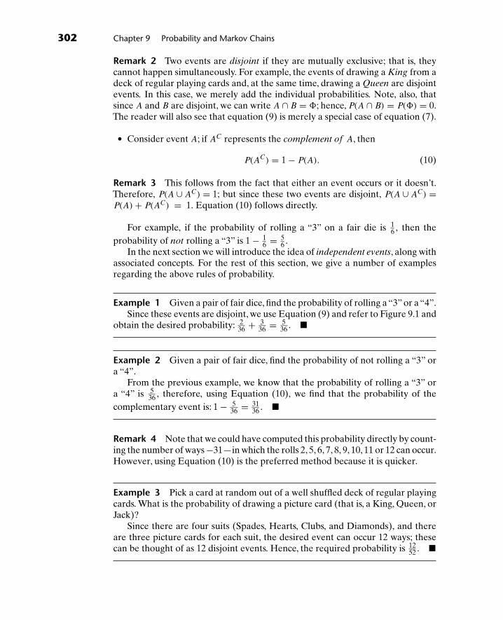
302 Chapter 9 Probability and Markov Chains
Remark 2 Two events are disjoint if they are mutually exclusive; that is, theycannot happen simultaneously. For example, the events of drawing a King from adeck of regular playing cards and, at the same time, drawing a Queen are disjointevents. In this case, we merely add the individual probabilities. Note, also, thatsince A and B are disjoint, we can write A ∩ B = �; hence, P(A ∩ B) = P(�) = 0.The reader will also see that equation (9) is merely a special case of equation (7).
● Consider event A; if AC represents the complement of A, then
P(AC) = 1 − P(A). (10)
Remark 3 This follows from the fact that either an event occurs or it doesn’t.Therefore, P(A ∪ AC) = 1; but since these two events are disjoint, P(A ∪ AC) =P(A) + P(AC) = 1. Equation (10) follows directly.
For example, if the probability of rolling a “3” on a fair die is 16 , then the
probability of not rolling a “3” is 1 − 16 = 5
6 .In the next section we will introduce the idea of independent events, along with
associated concepts. For the rest of this section, we give a number of examplesregarding the above rules of probability.
Example 1 Given a pair of fair dice, find the probability of rolling a “3” or a “4”.Since these events are disjoint, we use Equation (9) and refer to Figure 9.1 and
obtain the desired probability: 236 + 3
36 = 536 . �
Example 2 Given a pair of fair dice, find the probability of not rolling a “3” ora “4”.
From the previous example, we know that the probability of rolling a “3” ora “4” is 5
36 , therefore, using Equation (10), we find that the probability of thecomplementary event is: 1 − 5
36 = 3136 . �
Remark 4 Note that we could have computed this probability directly by count-ing the number of ways −31—in which the rolls 2, 5, 6, 7, 8, 9, 10, 11 or 12 can occur.However, using Equation (10) is the preferred method because it is quicker.
Example 3 Pick a card at random out of a well shuffled deck of regular playingcards. What is the probability of drawing a picture card (that is, a King, Queen, orJack)?
Since there are four suits (Spades, Hearts, Clubs, and Diamonds), and thereare three picture cards for each suit, the desired event can occur 12 ways; thesecan be thought of as 12 disjoint events. Hence, the required probability is 12
52 . �

9.2 Some Laws of Probability 303
Example 4 Pick a card at random out of a well shuffled deck of regular playingcards. Find the probability of drawing a red card or a picture card.
We know there are 12 picture cards as well as 26 red cards (Hearts or Dia-monds). But our events are not disjoint, since six of the picture cards arered. Therefore, we apply Equation (7) and compute the desired probability as1252 + 26
52 − 652 = 32
52 . �
Example 5 Suppose events A and B are not disjoint. Find P(A ∩ B), if it is giventhat P(A) = 0.4, P(B) = 0.3, and P(A ∪ B) = 0.6.
Recall Equation (7): P(A ∪ B) = P(A) + P(B) − P(A ∩ B). Therefore, 0.6 =0.4 + 0.3 − P(A ∩ B). Therefore, P(A ∩ B) = 0.1. �
Example 6 Extend formula (7) for three non-disjoint events. That is, considerP(A ∪ B ∪ C).
By using parentheses to group two events, we have the following equationbelow:
P(A ∪ B ∪ C) = P((A ∪ B) ∪ C) = P(A ∪ B) + P(C) − P((A ∪ B)) ∩ C). (11)
From Set Theory, we know that the last term of (11) can be written asP((A ∪ B) ∩ C) = P((A ∩ C) ∪ (B ∩ C)). Hence, applying (7) to (11) yields
P(A ∩ C) + P(B ∩ C) − P((A ∩ C) ∩ (B ∩ C)). (12)
But the last term of (12) is equivalent to P(A ∩ B ∩ C). After applying (7) tothe P(A ∪ B) term in (11), we have
P(A ∪ B ∪ C) = P(A) + P(B) + P(C) − P(A ∩ B)
− [P(A ∩ C) + P(B ∩ C) − P((A ∩ C) ∩ (B ∩ C))]. (13)
This simplifies to:
P(A ∪ B ∪ C) = P(A) + P(B) + P(C) − P(A ∩ B) − P(A ∩ C)
− P(B ∩ C) + P(A ∩ B ∩ C). (14)
�
Remark 5 Equation (14) can be extended for any finite number of events, andit holds even if some events are pairwise disjoint. For example, if events A and B
are disjoint, we merely substitute P(A ∩ B) = 0 into (14).

304 Chapter 9 Probability and Markov Chains
Problems 9.2
1. Pick a card at random from a well shuffled deck of regular playing cards. Findthe probabilities of:
a) Picking an Ace or a King.
b) Picking an Ace or a picture card.
c) Picking an Ace or a black card.
d) Picking the Four of Diamonds or the Six of Clubs.
e) Picking a red card or a Deuce.
f) Picking a Heart or a Spade.
g) Not choosing a Diamond.
h) Not choosing a Queen.
i) Not choosing an Ace or a Spade.
2. Roll a pair of fair dice. Find the probabilities of:
a) Getting an odd number.
b) Rolling a prime number.
c) Rolling a number divisible by four.
d) Not rolling a “7”.
e) Not rolling a “6” or an “8”.
f) Not rolling a “1”.
3. See Problem 2 of Section 9.1. Roll the three dice. Find the probabilities of:
a) Getting an odd number.
b) Rolling a “3”.
c) Rolling an “18”.
d) Rolling a “4”.
e) Rolling a “17”.
f) Rolling a “25”.
g) Not rolling a “4”.
h) Not rolling a “5”.
i) Not rolling a “6”.
4. Consider events A and B. Given P(A) = .7 and P(B) = .2, find the probabilityof “A or B” if P(A ∩ B) = .15.

9.3 Bernoulli Trials and Combinatorics 305
5. Suppose events A and B are equally likely. Find their probabilities if P(A ∪ B) =.46 and P(A ∩ B) = .34.
6. Extend Equation (14) for any four events A, B, C, and D.
9.3 Bernoulli Trials and Combinatorics
In the previous section, we considered single events. For example, rolling dice onceor drawing one card out of a deck. In this section we consider multiple events whichneither affect nor are affected by preceding or succeeding events.
For this section, we will consider events with only two outcomes. For example,flipping a coin, which can result in only “heads” or “tails”. The coin cannot land onits edge. We do not insist that the probability of a “head” equals the probabilityof a “tail”, but we will assume that the probabilities remain constant. Each one ofthe “flips” will be called a Bernoulli trial, in honor of Jakob Bernoulli (1654–1705).
Remark 1 A closely related underlying mathematical structure for these trialsis known as a Binomial Distribution.
Remark 2 The Bernoulli family had a number of great mathematicians andscientists spanning several generations. This family is to mathematics what theBach family is to music.
As we have indicated, we will assume that the events are independent. Hencethe probabilities are unaffected at all times. So, if we tossed a coin 10 times in arow, each of the tosses would be called a Bernoulli trial, and the probability ofgetting a head on each toss would remain constant.
We will assume the following rule. If two events, A and B, are independent,then the probability of “A and B” or the probability of “A followed by B” is givenby:
P(AB) = P(A ∩ B) = P(A)P(B). (15)
Notice that we use the intersection (∩) notation. This simple rule is called themultiplication rule.
Remark 3 The reader must be careful not to confuse disjoint events with inde-pendent events. The former means that “nothing is in common” or that the events“cannot happen simultaneously”. The latter means that the probabilities do notinfluence one another. Often, but not always, independent events are sequential;like flipping a coin 10 times in a row.
It is clear that probabilities depend on counting, as in determining the size ofthe sample space. We assume the following result from an area of mathematics

306 Chapter 9 Probability and Markov Chains
known as Combinatorics:
● The number of ways we can choose k objects from a given collection of n objectsis given by: (
n
k
)= n!
k!(n − k)! . (16)
Remark 4 This is equivalent to determining the number of subsets of size k givena set of size n, where k ≤ n.
Remark 5 We saw “factorials” in Chapter Seven. Recall that 3!, for example,is read “three factorial” and it is evaluated 3 · 2 · 1 = 6. Hence, “n − factorial” isgiven by n! = n(n − 1)(n − 2) · · · 3 · 2 · 1. By convention, we define 0! = 1. Finally,we only consider cases where n is a non-negative integer.
Remark 6 For these “number of ways”, we are not concerned about the orderof selection. We are merely interested in the number of combinations (as opposedto the number of permutations).
We will provide the reader with a number of examples which illustrate thesalient points of this section.
Example 1 Evaluate(
52
). Using (16) we see that
(52
)= 5!
2!(5−2)! = 5!2!3! .
Since 5! = 120, 2! = 2 and 3! = 6,(
52
)= 120
12 = 10. �
Example 2 Given a committee of five people, in how many ways can a sub-committee of size two be formed? The number is precisely what we computedin the previous example: 10. The reader can verify this as follows. Suppose thepeople are designated: A, B, C, D, and E. Then, the 10 sub-committees of size twoare given by: AB, AC, AD, AE, BC, BD, BE, CD, CE, and DE. �
Example 3 Given a committee of five people, in how many ways can a sub-committee of size three be formed? We can use formula (16) to compute theanswer, however the answer must be 10. This is because a sub-committee of 3 isthe complement of a sub-committee or two. That is, consider the three people noton a particular sub-committee of two, as constituting a sub-committee of three.For example, if A and B are on one sub-committee of size two, put C, D, and E ona sub-committee of size three. Clearly there are 10 such pairings. �
Example 4 Suppose we flip a fair coin twice. What is the probability of gettingexactly one “head”?

9.3 Bernoulli Trials and Combinatorics 307
Let H represent getting a“head”and T represent getting a“tail”. Since the coinis fair, P(H) = P(T) = 1
2 . The only way we can obtain exactly one head in two tossesis if the order of outcomes is either HT or TH . Note that the events are disjointor mutually exclusive; that is, we cannot get these two outcomes at the same time.Hence, Equation (9) will come into play. And because of the independence of thecoin flips (each toss is a Bernoulli trial), we will use Equation (15) to determinethe probability of obtaining HT and TH .
Therefore, the probability of getting exactly one H is equal to
P(HT ∪ TH) = P(HT ) + P(TH) = P(H)P(T ) + P(T )P(H)
= 12
· 12
+ 12
· 12
= 12.
(17)
�
Remark 7 Note that (17) could have been obtained by finding the probability ofHT —in that order—and then multiplying it by the number of times (combinations)we could get exactly one H in two tosses.
Example 5 Now, suppose we flip a fair coin 10 times. What is the probability ofgetting exactly one “head”?
Suppose we get the H on the first toss. Then the probability of getting
HTTTTTTTTT —in that order—is equal to(
12
)·(
12
)9 = 11024 , because the tosses
are all independent. Note that if the H occurs “in the second slot”, the probabilityis also 1
1024 . In fact, we get the same number for all 10 possible “slots”. Hence thefinal answer to our question is 10
1024 . �
Remark 8 Note that the previous example could have be answered by thefollowing computation
(101
)(12
)(12
)9
= 101024
. (18)
Here, the first factor gives the number of ways we can get exactly one H
in 10 tosses; this is where mutual exclusivity comes in. The second factor is theprobability of getting one H , and the third factor is the probability of getting nineT s; the independence factor is employed here.
Example 6 Suppose we flip a fair coin 10 times. Find the probability of gettingexactly five Hs.

308 Chapter 9 Probability and Markov Chains
Since there are(
105
)= 252 ways of getting five Hs in 10 tosses, the desired
probability is given by
(105
)(12
)5 (12
)5
= 2521024
. (19)
�
Example 7 Suppose we flip an unfair coin 10 times. If P(H) = .3 and the P(T ) =.7, what is the probability of getting exactly five Hs?
As we learned from the previous problem, there are 252 ways of getting exactlyfive Hs in 10 tosses. Hence, our desired probability is given by
(105
)(.3)5(.7)5 ≈ 0.103. �
Remark 9 A calculator is useful for numerical computations. We will addressthe issues of calculations and technology in both Section 9.5 and in the Appendix.Note, too, that individual probabilities, P(H) and P(T ) must add to 1, and thatthe exponents in the formula must add to the total number of tosses; in thiscase, 10.
Example 8 Consider the previous example. Find the probability of getting atleast five Hs.
Note that at least five Hs means exactly five Hs plus exactly six Hs plus … etc.Note, also, that exactly five Hs and exactly six Hs are disjoint, so we will useEquation (9). Therefore the desired probability is given by:
(105
)(.3)5(.7)5 +
(106
)(.3)6(.7)4 +
(107
)(.3)7(.7)3 +
(108
)(.3)8(.7)2
+(
109
)(.3)9(.7)1 +
(1010
)(.3)10(.7)10 ≈ 0.150. (20)
�
Example 9 Consider the previous examples. Find the probability of getting atleast one H .

9.3 Bernoulli Trials and Combinatorics 309
While we could follow the approach in Example 9, there is a simpler way toanswer this question. If we realize that the complement of the desired event isgetting no Hs in 10 tosses, we can apply Equation (10). That is, the probability ofgetting at least one H is equal to
1 −(
100
)(.3)0(.7)10 ≈ 0.972. (21)
�
We summarize the results for the probability in this section as follows:
● Given n successive Bernoulli trials, the probability of getting exactly k
successes, where k ≤ n, is equal to
n!k!(n − k)!p
k(1 − p)n−k (22)
where the probability of a success is p, and the probability of a failure is (1 − p).
Problems 9.3
1. Evaluate the following:
a)(
62
); b)
(71
); c)
(85
); d)
(2018
); e)
(202
);
f)(
10001000
); g)
(1000
0
); h)
(10099
); i)
(1000999
); j)
(00
).
2. How many different nine-player line-ups can the New York Yankees produceif there are 25 players on the roster and every player can play every position?
3. Suppose 15 women comprised a club, and a committee of 6 members wasneeded. How many different committees would be possible?
4. Toss a fair die eight times. Find the probability of:
a) Rolling exactly one “5”.
b) Rolling exactly three “5s”.
c) Rolling at least three “5s”.
d) Rolling at most three “5s”.
e) Rolling at least one “5”.
5. Suppose event A has a probability of occurring equal to .65. Without evalu-ating the expressions, find the following probabilities given 500 independentBernoulli trials.

310 Chapter 9 Probability and Markov Chains
a) Event A occurs 123 times.
b) Event A occurs 485 times.
c) Event A occurs at least 497 times.
d) Event A occurs at most 497 times.
e) Event A occurs any non-zero multiple of 100 times.
6. An urn contains 10 golf balls, three of which are white, with the remainingseven painted orange. A blindfolded golfer picks a golf ball from the urn, andthen replaces it. The process is repeated nine times, making a total of 10 trials.What is the probability of the golfer picking a white golf ball exactly threetimes?
7. An urn contains 10 golf balls colored as follows: three are white; two are green;one is red; four are orange. A blindfolded golfer picks a golf ball from the urn,and then replaces it. The process is repeated nine times, making a total of 10trials. What is the probability of the golfer picking a white golf ball exactlythree times?
9.4 Modeling with Markov Chains: An Introduction
In Chapter 1 and Chapter 6, we mentioned the concept of Markov chains. Wereturn to this idea, further formalizing it from the perspective of probability.Consider the following example, which we will call the Moving Situation.
Example 1 Suppose we have two families. Family (1) lives in state A and Family(2) lives in state B. Let us further assume that the matrix
P =[.7 .3.9 .1
](23)
represents the following probabilities. The element in the first row and first columnrepresents the probability of Family (1) originally residing in state A remainingin state A, while the element in the first row and second column represents theprobability of starting in state A and then moving to state B. Note that these twoprobabilities add to one.
Similarly, let the element in the second row and first column, represent theprobability of Family (2) starting in state B and moving to state A, while the ele-ment in the second row and second column, represents the probability of startingin state B and remaining in state B. Here, too, these two probabilities add to one.
Note that we can consider the process as “time conditioned” in the sense thatthere is a present and a future (for example, one year from the present).
Such a matrix is called a transition matrix and the elements are calledtransitional probabilities.

9.4 Modeling with Markov Chains: An Introduction 311
Let us consider the matrix in (23) and let us compute P2. We find that
P2 =[.76 .24.72 .28
]. (24)
What does P2 represent? To answer this question, let us ask another question:From the perspective of Family (1), what is the probability of being in state A aftertwo years?
There are two ways Family (1) can be in state A after two years:
● Scenario 1: Either the family stayed two years in a row.
● Scenario 2: The family moved to state B after one year and then moved backto state A after the second year.
The probability of the first scenario is .7(.7) = .49, because these events can beconsidered independent. The probability of the second is .3(.7) = .27.
Because these events are disjoint, we add the probabilities to get .76.Note that this is the element in the first row and first column of P2.By similar analyses we find that P2 is indeed the transitional matrix of our
Moving Situation after two time periods.Matrix P is the transition matrix for a Markov chain. The sum of the proba-
bilities of each row must add to one, and by the very nature of the process, thematrix must be square. We assume that at any time each object is in one and onlyone state (although different objects can be in the same state). We also assumethat the probabilities remain constant over the given time period. �
Remark 1 The notation p(n)ij is used to signify the transitional probability of
moving from state i to state j over n time periods.
Example 2 Suppose Moe, Curly, and Larry live in the same neighborhood. Letthe transition matrix
S =⎡⎣.7 .1 .2
.5 .3 .2
.8 .1 .1
⎤⎦ (25)
represent the respective probabilities of Moe, Curly, and Larry staying at homeon Monday and either visiting one of their two neighbors or staying home onTuesday. We ask the following questions regarding Thursday:
a) What is the probability of Moe going to visit Larry at his home, p(3)13?
b) What is the probability of Curly being at his own home, p(3)22?

312 Chapter 9 Probability and Markov Chains
To answer both of these questions, we must compute P3 because three timeperiods would have elapsed. We find that
P3 =⎡⎣.694 .124 .182
.124 .132 .182
.695 .124 .181
⎤⎦ . (26)
So, our answers are as follows: a) the probability is .182, the entry in the firstrow and third column; b) the probability is .132, the entry in the second row andsecond column. �
Example 3 Consider the transitional matrix K which represents respectiveprobabilities of Republicans, Democrats, and Independents either remainingwithin their political parties or changing their political parties over a two-yearperiod:
K =⎡⎣ .7 .1 .2
.15 .75 .1.3 .2 .5
⎤⎦. (27)
What is the probability of a Republican becoming an Independent after four years?And what is the probability of a Democrat becoming a Republican after fouryears?
Both of these questions require two time periods; hence we need p(2)13 and
p(2)21 which can be obtained from K2 below:
K2 =⎡⎣ .565 .185 .25
.2475 .5975 .155.39 .28 .33
⎤⎦. (28)
Hence, p(2)13 = .25 and p(2)
21 = .2475.We close this discussion with the observation that sometimes transitional
matrices have special properties. For example, consider the matrix
A =[.5 .5.3 .7
]. (29)
We find that if we raise this matrix to the 9th and 10th powers, our result is thesame. That is,
A9 = A10 =[.375 .625.375 .625
]. (30)
and the same result occurs for any higher power of A. This absorbing qualityimplies that “sooner or later” the transitional probabilities will stabilize.

9.4 Modeling with Markov Chains: An Introduction 313
Markov processes are used in many areas including decision theory, economicsand political science. �
Problems 9.4
1. Why are the following matrices not transitional matrices?
a)[
0 1−1 2
]; b)
[.6 .5.4 .5
]; c)
⎡⎣.1 .2 .7
1 0 00 0 0
⎤⎦; d)
[.1 .5 .4.2 .6 .2
]
2. Consider the following transitional matrices. Construct scenarios for whichthese matrices might represent the transitional probabilities:
a)[.5 .5.7 .3
]; b)
[.95 .05.02 .98
]; c)
[.5 .5.5 .5
];
d)[
1 00 .1
]; e)
[0 11 0
]; f)
⎡⎣.1 .2 .7
.5 .25 .25
.3 .3 .4
⎤⎦
3. Consider the c) and d) matrices in the previous problem; show that thesematrices are “absorbing” matrices.
4. Consider the e) matrix in Problem (2). Raise the matrix to the powers of 2, 3,4, 5, 6, 7, and 8. What do you notice? Can you construct a scenario for whichthis transitional matrix could be a model?
5. Consider the following transitional matrix:[.6 .4.1 .9
]. Find p(2)
11, p(2)21, p(3)
12,
and p(3)22.
6. Consider a game called Red-Blue. The rules state that after one “turn” Red canbecome Blue or remain Red. The same is true with Blue. Suppose you make abet that after five turns, Red will be in the Red category. You are told that thefollowing probabilities are valid:
● Given Red, the probability of remaining Red after one turn is .7
● Given Red, the probability of going to Blue is .3
● Given Blue, the probability of remaining Blue is .6
● Given Blue, the probability of going to Red is .4
a) Give the transition matrix.
b) What is the probability of you winning your bet?
c) Does the probability increase, decrease or stay the same if you bet six turnsinstead of five?

314 Chapter 9 Probability and Markov Chains
9.5 Final Comments on Chapter 9
Probability is a fascinating area. For numbers that necessarily range between 0and 1, inclusively, a lot can happen.
When using probability, we must understand exactly what is being asked andgive precise answers, without misrepresenting our conclusions. Concepts such asrandomness and independence must be present before certain laws can be applied.While the mathematical underpinnings are rock solid, probabilities generally dealwith “trends” and “likelihoods”.
Regarding Bernoulli trials, if the number of experiments is large, the calcu-lations can be overwhelming. In these cases, the use of computers and othertechnological aids is essential. From a theoretical perspective, there is a very goodapproximation that can be employed, known as the Normal Approximation to theBinomial Distribution. This technique is explored in basic courses on probabilityand statistics.
One final point: With the exception of the section on Markov chains, all theprobabilities in Chapter 9 were theoretically assigned. That is, we made assump-tions, applied definitions and then made our computations. For example, if a diewas fair, then we assigned a probability of 1
6 to the event of rolling a “3”, based onour definition, which dealt with relative frequency.
However, there are many times when probabilities are obtained by observationand empirical evidence. For example, the greatest baseball player of all time, BabeRuth, had a lifetime batting average of .342. Since batting average is defined assuccessful hits divided by total at-bats, we can interpret this as Ruth getting 342hits for every 1000 at-bats over a long period of time.
There are many other occurrences of empirical probabilities in research areassuch as medicine, psychology, economics, and sociology, to name but a few.

1010Real Inner Products andLeast-Square
10.1 Introduction
To any two vectors x and y of the same dimension having real components (asdistinct from complex components), we associate a scalar called the inner product,denoted as 〈x, y〉, by multiplying together the corresponding elements of x and y,and then summing the results. Students already familiar with the dot product oftwo- and three-dimensional vectors will undoubtedly recognize the inner productas an extension of the dot product to real vectors of all dimensions.
Example 1 Find 〈x, y〉 if
x =⎡⎣1
23
⎤⎦ and y =
⎡⎣ 4
−56
⎤⎦.
Solution 〈x, y〉 = 1(4) + 2(−5) + 3(6) = 12. �
Example 2 Find 〈u, v〉 if u = [20 −4 30 10] and v = [10 −5 −8 −6].
Solution 〈u, v〉 = 20(10) + (−4)(−5) + 30(−8) + 10(−6) = −80. �
It follows immediately from the definition that the inner product of real vectorssatisfies the following properties:
(I1) 〈x, x〉 is positive if x �= 0; 〈x, x〉 = 0 if and only if x = 0.
(I2) 〈x, y〉 = 〈y, x〉.(I3) 〈λx, y〉 = λ〈x, y〉, for any real scalar λ.
315

316 Chapter 10 Real Inner Products and Least-Square
(I4) 〈x + z, y〉 = 〈x, y〉 + 〈z, y〉.(I5) 〈0, y〉 = 0.
We will only prove (I1) here and leave the proofs of the other propertiesas exercises for the students (see Problems 29 through 32). Let x =[x1 x2 x3 · · · xn] be an n-dimensional row vector whose componentsx1, x2, x3, . . . , xn are all real. Then,
〈x, x〉 = (x1)2 + (x2)
2 + (x3)2 + · · · + (xn)
2.
This sum of squares is zero if and only if x1 = x2 = x3 = · · · = xn = 0, which inturn implies x = 0. If any one component is not zero, that is, if x is not the zerovector, then the sum of squares must be positive.
The inner product of real vectors is related to the magnitude of a vector asdefined in Section 1.6. In particular,
‖x‖ = √〈x, x〉.
Example 3 Find the magnitude of x = [2 −3 −4].
Solution 〈x, x〉 = 2(2) + (−3)(−3) + (−4)(−4) = 29, so the magnitude of x is
‖x‖ = √29. �
The concepts of a normalized vector and a unit vector are identical to thedefinitions given in Section 1.6. A nonzero vector is normalized if it is divided byits magnitude. A unit vector is a vector whose magnitude is unity. Thus, if x is anynonzero vector, then (1/‖x‖) x is normalized. Furthermore,
〈 1‖x‖x,
1‖x‖x〉 = 1
‖x‖〈x,1
‖x‖x〉 (Property I3)
= 1‖x‖〈 1
‖x‖x, x〉 (Property I2)
=(
1‖x‖
)2
〈x, x〉 (Property I3)
=(
1‖x‖
)2
‖x‖2 = 1,
so a normalized vector is always a unit vector.

10.1 Introduction 317
Problems 10.1
In Problems 1 through 17, find (a) 〈x, y〉 and (b) 〈x, x〉 for the given vectors.
1. x =[
12
]and y =
[34
].
2. x =[
20
]and y =
[4
−5
].
3. x =[−5
7
]and y =
[3
−5
].
4. x = [3 14] and y = [7 3].5. x = [−2 −8] and y = [−4 −7].
6. x =⎡⎣2
01
⎤⎦ and y =
⎡⎣1
24
⎤⎦.
7. x =⎡⎣−2
2−4
⎤⎦ and y =
⎡⎣−4
3−3
⎤⎦.
8. x =⎡⎣−3
−25
⎤⎦ and y =
⎡⎣ 6
−4−4
⎤⎦.
9. x = [ 12
13
16
]and y = [ 1
332 1
].
10. x = [1/√
2 1/√
3 1/√
6]
and y = [1/√
3 3/√
2 1].
11. x = [ 13
13
13
]and y = [ 1
412
18
].
12. x = [10 20 30] and y = [5 −7 3].
13. x =
⎡⎢⎢⎣
1011
⎤⎥⎥⎦ and y =
⎡⎢⎢⎣
1101
⎤⎥⎥⎦.
14. x =
⎡⎢⎢⎢⎢⎢⎣
12121212
⎤⎥⎥⎥⎥⎥⎦ and y =
⎡⎢⎢⎣
123
−4
⎤⎥⎥⎦.
15. x =
⎡⎢⎢⎣
35
−7−8
⎤⎥⎥⎦ and y =
⎡⎢⎢⎣
4−6−9
8
⎤⎥⎥⎦.

318 Chapter 10 Real Inner Products and Least-Square
16. x = [ 15
15
15
15
15
]and y = [1 2 −3 4 −5
].
17. x = [1 1 1 1 1 1] and y = [−3 8 11 −4 7].18. Normalize y as given in Problem 1.
19. Normalize y as given in Problem 2.
20. Normalize y as given in Problem 4.
21. Normalize y as given in Problem 7.
22. Normalize y as given in Problem 8.
23. Normalize y as given in Problem 11.
24. Normalize y as given in Problem 15.
25. Normalize y as given in Problem 16.
26. Normalize y as given in Problem 17.
27. Find x if 〈x, a〉b = c, where
a =⎡⎣ 1
3−1
⎤⎦, b =
⎡⎣2
11
⎤⎦, and c =
⎡⎣ 3
0−1
⎤⎦.
28. Determine whether it is possible for two nonzero vectors to have an innerproduct that is zero.
29. Prove Property I2.
30. Prove Property I3.
31. Prove Property I4.
32. Prove Property I5.
33. Prove that ‖x + y‖2 = ‖x‖2 + 2〈x, y〉 + ‖y‖2.
34. Prove the parallelogram law:
‖x + y‖2 + ‖x − y‖2 = 2‖x‖2 + 2‖y‖2.
35. Prove that, for any scalar λ,
0 ≤ ‖λx − y‖2 = λ2‖x‖2 − 2λ〈x, y〉 + ‖y‖2.
36. (Problem 35 continued) Take λ = 〈x, y〉/‖x‖2 and show that
0 ≤ −〈x, y〉2
‖x‖2 + ‖y‖2.

10.1 Introduction 319
From this, deduce that
〈x, y〉2 ≤ ‖x‖2‖y‖2,
and that
|〈x, y〉| ≤ ‖x‖ ‖y‖.
This last inequality is known as the Cauchy–Schwarz inequality.
37. Using the results of Problem 33 and the Cauchy–Schwarz inequality, showthat
‖x + y‖2 ≤ ‖x‖2 + 2‖x‖‖y‖ + ‖y‖2
= (‖x‖ + ‖y‖)2.
From this, deduce that
‖x + y‖ ≤ ‖x‖ + ‖y‖.
38. Determine whether there exists a relationship between 〈x, y〉 and xTy, whenboth x and y are column vectors of identical dimension with real components.
39. Use the results of Problem 38 to prove that 〈Ax, y〉 = 〈x, ATy〉, when A, x,and y are real matrices of dimensions n × n, n × 1, and n × 1, respectively.
40. A generalization of the inner product for n-dimensional column vectors withreal components is 〈x, y〉A = 〈Ax, Ay〉 for any real n × n nonsingular matrixA. This definition reduces to the usual one when A = I.
Compute 〈x, y〉A for the vectors given in Problem 1 when
A =[
2 31 −1
].
41. Compute 〈x, y〉A for the vectors given in Problem 6 when
A =⎡⎣1 1 0
1 0 10 1 1
⎤⎦.
42. Redo Problem 41 with
A =⎡⎣1 −1 1
0 1 −11 1 1
⎤⎦.

320 Chapter 10 Real Inner Products and Least-Square
10.2 Orthonormal Vectors
Definition 1 Two vectors x and y are orthogonal (or perpendicular) if 〈x, y〉 = 0.Thus, given the vectors
x =⎡⎣1
11
⎤⎦, y =
⎡⎣−1
10
⎤⎦, z =
⎡⎣1
10
⎤⎦,
we see that x is orthogonal to y and y is orthogonal to z since 〈x, y〉 = 〈y, z〉 = 0;but the vectors x and z are not orthogonal since 〈x, z〉 = 1 + 1 �= 0. In particular,as a direct consequence of Property (I5) of Section 10.1 we have that the zerovector is orthogonal to every vector.
A set of vectors is called an orthogonal set if each vector in the set is orthogonalto every other vector in the set. The set given above is not an orthogonal set sincez is not orthogonal to x whereas the set given by {x, y, z},
x =⎡⎣1
11
⎤⎦, y =
⎡⎣ 1
1−2
⎤⎦, z =
⎡⎣ 1
−10
⎤⎦,
is an orthogonal set because each vector is orthogonal to every other vector.
Definition 2 A set of vectors is orthonormal if it is an orthogonal set having theproperty that every vector is a unit vector (a vector of magnitude 1).
The set of vectors ⎧⎨⎩⎡⎣1/
√2
1/√
20
⎤⎦,
⎡⎣ 1/
√2
−1/√
20
⎤⎦,
⎡⎣0
01
⎤⎦⎫⎬⎭
is an example of an orthonormal set.Definition 2 can be simplified if we make use of the Kronecker delta, δij,
defined by
δij ={
1 if i = j,
0 if i �= j.(1)
A set of vectors {x1, x2, . . . , xn} is an orthonormal set if and only if⟨xi, xj
⟩ = δij for all i and j, i, j = 1, 2, . . . , n. (2)
The importance of orthonormal sets is that they are almost equivalent to lin-early independent sets. However, since orthonormal sets have associated withthem the additional structure of an inner product, they are often more conve-nient. We devote the remaining portion of this section to showing the equivalenceof these two concepts. The utility of orthonormality will become self-evident inlater sections.

10.2 Orthonormal Vectors 321
Theorem 1 An orthonormal set of vectors is linearly independent.
Proof. Let {x1, x2, . . . , xn} be an orthonormal set and consider the vectorequation
c1x1 + c2x2 + · · · + cnxn = 0 (3)
where the cj’s (j = 1, 2, . . . , n) are constants. The set of vectors will be linearlyindependent if the only constants that satisfy (3) are c1 = c2 = · · · = cn = 0. Takethe inner product of both sides of (3) with x1. Thus,
〈c1x1 + c2x2 + · · · + cnxn, x1〉 = 〈0, x1〉 .
Using properties (I3), (I4), and (I5) of Section 10.1, we have
c1〈x1, x1〉 + c2〈x2, x1〉 + · · · + cn〈xn, x1〉 = 0.
Finally, noting that 〈xi, x1〉 = δi1, we obtain c1 = 0. Now taking the inner prod-uct of both sides of (3) with x2, x3, . . . , xn, successively, we obtain c2 = 0,
c3 = 0, . . . , cn = 0. Combining these results, we find that c1 = c2 = · · · cn = 0,which implies the theorem.
Theorem 2 For every linearly independent set of vectors {x1, x2, . . . , xn}, thereexists an orthonormal set of vectors {q1, q2, . . . , qn} such that each qj(j =1, 2, . . . , n) is a linear combination of x1, x2, . . . , xj .
Proof. First define new vectors y1, y2, . . . , yn by
y1 = x1
y2 = x2 − 〈x2, y1〉〈y1, y1〉y1
y3 = x3 − 〈x3, y1〉〈y1, y1〉y1 − 〈x3, y2〉
〈y2, y2〉y2
and, in general,
yj = xj −j−1∑k=1
〈xj, yk〉〈yk, yk〉yk (j = 2, 3, . . . , n). (4)
Each yj is a linear combination of x1, x2, . . . , xj(j = 1, 2, . . . , n). Since the x’s arelinearly independent, and the coefficient of the xj term in (4) is unity, it followsthat yj is not the zero vector (see Problem 19). Furthermore, it can be shown thatthe yj terms form an orthogonal set (see Problem 20), hence the only property

322 Chapter 10 Real Inner Products and Least-Square
that the yj terms lack in order to be the required set is that their magnitudes maynot be one. We remedy this situation by defining
qj = yj
‖yj‖ . (5)
The desired set is {q1, q2, . . . , qn}.The process used to construct the qj terms is called the Gram–Schmidt
orthonormalization process.
Example 1 Use the Gram–Schmidt orthonormalization process to constructan orthonormal set of vectors from the linearly independent set {x1, x2, x3},where
x1 =⎡⎣1
10
⎤⎦, x2 =
⎡⎣0
11
⎤⎦, x3 =
⎡⎣1
01
⎤⎦.
Solution
y1 = x1 =⎡⎣1
10
⎤⎦.
Now 〈x2, y1〉 = 0(1) + 1(1) + 1(0) = 1, and 〈y1, y1〉 = 1(1) + 1(1) + 0(0) = 2;hence,
y2 = x2 − 〈x2, y1〉〈y1, y1〉y1 = x2 − 1
2y1 =
⎡⎣0
11
⎤⎦− 1
2
⎡⎣1
10
⎤⎦ =
⎡⎣−1/2
1/21
⎤⎦.
Then,
〈x3, y1〉 = 1(1) + 0(1) + 1(0) = 1,
〈x3, y2〉 = 1(−1/2) + 0 (1/2) + 1(1) = 1/2,
〈y2, y2〉 = (−1/2)2 + (1/2)2 + (1)2 = 3/2,
so
y3 = x3 − 〈x3, y1〉〈y1, y1〉y1 − 〈x3, y2〉
〈y2, y2〉y2 = x3 − 12
y1 − 1/23/2
y2
=⎡⎣1
01
⎤⎦− 1
2
⎡⎣1
10
⎤⎦− 1
3
⎡⎣−1/2
1/21
⎤⎦ =
⎡⎣ 2/3
−2/32/3
⎤⎦.

10.2 Orthonormal Vectors 323
The vectors y1, y2, and y3 form an orthogonal set. To make this set orthonormal, wenote that 〈y1, y1〉 = 2, 〈y2, y2〉 = 3/2, and 〈y3, y3〉 = (2/3)(2/3) + (−2/3)(−2/3) +(2/3)(2/3) = 4/3. Therefore,
‖y1‖ = √〈y1, y1〉 = √2 ‖y2‖ = √〈y2, y2〉 = √3/2,
‖y3‖ = √〈y3, y3〉 = 2/√
3,
and
q1 = y1
‖y1‖ = 1√2
⎡⎣1
10
⎤⎦ =
⎡⎣1/
√2
1/√
20
⎤⎦,
q2 = y2
‖y2‖ = 1√3/2
⎡⎣−1/2
1/21
⎤⎦ =
⎡⎣−1/
√6
1/√
62/
√6
⎤⎦,
q3 = y3
‖y3‖ = 1
2/√
3
⎡⎣ 2/3
−2/32/3
⎤⎦ =
⎡⎣ 1/
√3
−1/√
31/
√3
⎤⎦. �
Example 2 Use the Gram–Schmidt orthonormalization process to construct anorthonormal set of vectors from the linearly independent set {x1, x2, x3, x4}, where
x1 =
⎡⎢⎢⎣
1101
⎤⎥⎥⎦, x2 =
⎡⎢⎢⎣
1210
⎤⎥⎥⎦, x3 =
⎡⎢⎢⎣
0121
⎤⎥⎥⎦, x4 =
⎡⎢⎢⎣
1011
⎤⎥⎥⎦.
Solution
y1 = x1 =
⎡⎢⎢⎣
1101
⎤⎥⎥⎦,
〈y1, y1〉 = 1(1) + 1(1) + 0(0) + 1(1) = 3,
〈x2, y1〉 = 1(1) + 2(1) + 1(0) + 0(1) = 3,
y2 = x2 − 〈x2, y1〉〈y1, y1〉y1 = x2 − 3
3y1 =
⎡⎢⎢⎣
011
−1
⎤⎥⎥⎦;

324 Chapter 10 Real Inner Products and Least-Square
〈y2, y2〉 = 0(0) + 1(1) + 1(1) + (−1)(−1) = 3,
〈x3, y1〉 = 0(1) + 1(1) + 2(0) + 1(1) = 2,
〈x3, y2〉 = 0(0) + 1(1) + 2(1) + 1(−1) = 2,
y3 = x3 − 〈x3, y1〉〈y1, y1〉y1 − 〈x3, y2〉
〈y2, y2〉y2
= x3 − 23
y1 − 23
y2 =
⎡⎢⎢⎣
−2/3−1/3
4/31
⎤⎥⎥⎦;
〈y3, y3〉 =(−2
3
)2
+(−1
3
)2
+(
43
)2
+ (1)2 = 103
,
〈x4, y1〉 = 1(1) + 0(1) + 1(0) + 1(1) = 2,
〈x4, y2〉 = 1(0) + 0(1) + 1(1) + 1(−1) = 0,
〈x4, y3〉 = 1(−2
3
)+ 0(−1
3
)+ 1(
43
)+ 1(1) = 5
3,
y4 = x4 − 〈x4, y1〉〈y1, y1〉y1 − 〈x4, y2〉
〈y2, y2〉y2 − 〈x4, y3〉〈y3, y3〉y3
= x4 − 23
y1 − 03
y2 − 5/310/3
y3 =
⎡⎢⎢⎣
2/3−1/2
1/3−1/6
⎤⎥⎥⎦.
Then
〈y4, y4〉 = (2/3)(2/3) + (−1/2)(−1/2) + (1/3)(1/3) + (−1/6)(−1/6)
= 5/6,
and
q1 = 1√3
⎡⎢⎢⎣
1101
⎤⎥⎥⎦ =
⎡⎢⎢⎣
1/√
31/
√3
01/
√3
⎤⎥⎥⎦,
q2 = 1√3
⎡⎢⎢⎣
011
−1
⎤⎥⎥⎦ =
⎡⎢⎢⎣
01/
√3
1/√
3−1/
√3
⎤⎥⎥⎦,

10.2 Orthonormal Vectors 325
q3 = 1√10/3
⎡⎢⎢⎣
−2/3−1/3
4/31
⎤⎥⎥⎦ =
⎡⎢⎢⎣
−2/√
30−1/
√30
4/√
303/
√30
⎤⎥⎥⎦,
q4 = 1√5/6
⎡⎢⎢⎣
2/3−1/2
1/3−1/6
⎤⎥⎥⎦ =
⎡⎢⎢⎣
4/√
30−3/
√30
2/√
30−1/
√30
⎤⎥⎥⎦. �
Problems 10.2
1. Determine which of the following vectors are orthogonal:
x =[
12
], y =
[2
−1
], z =
[−2−1
], u =
[−42
], v =
[36
].
2. Determine which of the following vectors are orthogonal:
x =⎡⎣1
12
⎤⎦, y =
⎡⎣1
11
⎤⎦, z =
⎡⎣ 1
1−1
⎤⎦, u =
⎡⎣ 1
−10
⎤⎦, v =
⎡⎣−2
11
⎤⎦.
3. Find x so that [35
]is orthogonal to
[x
4
].
4. Find x so that ⎡⎣−1
x
3
⎤⎦ is orthogonal to
⎡⎣1
23
⎤⎦.
5. Find x so that [x x 2] is orthogonal to [1 3 − 1].
6. Find x and y so that [x y] is orthogonal to [1 3].
7. Find x and y so that
⎡⎣x
y
1
⎤⎦ is orthogonal to both
⎡⎣1
23
⎤⎦ and
⎡⎣1
11
⎤⎦.

326 Chapter 10 Real Inner Products and Least-Square
8. Find x, y, and z so that
⎡⎣x
y
z
⎤⎦ is orthogonal to both
⎡⎣1
01
⎤⎦ and
⎡⎣1
12
⎤⎦.
9. Redo Problem 8 with the additional stipulation that [x y z]ᵀ be a unitvector.
In Problems 10 through 18, use the Gram–Schmidt orthonormalization processto construct an orthonormal set from the given set of linearly independent vectors.
10. x1 =[
12
], x2 =
[21
]. 11. x1 =
[11
], x2 =
[35
].
12. x1 =[
3−2
], x2 =
[33
].
13. x1 =⎡⎣1
21
⎤⎦, x2 =
⎡⎣1
01
⎤⎦, x3 =
⎡⎣1
02
⎤⎦.
14. x1 =⎡⎣2
10
⎤⎦, x2 =
⎡⎣0
11
⎤⎦, x3 =
⎡⎣2
02
⎤⎦.
15. x1 =⎡⎣1
10
⎤⎦, x2 =
⎡⎣2
01
⎤⎦, x3 =
⎡⎣2
21
⎤⎦.
16. x1 =⎡⎣0
34
⎤⎦, x2 =
⎡⎣3
50
⎤⎦, x3 =
⎡⎣2
55
⎤⎦.
17. x1 =
⎡⎢⎢⎣
0111
⎤⎥⎥⎦, x2 =
⎡⎢⎢⎣
1011
⎤⎥⎥⎦, x3 =
⎡⎢⎢⎣
1101
⎤⎥⎥⎦, x4 =
⎡⎢⎢⎣
1110
⎤⎥⎥⎦.
18. x1 =
⎡⎢⎢⎣
1100
⎤⎥⎥⎦, x2 =
⎡⎢⎢⎣
01
−10
⎤⎥⎥⎦, x3 =
⎡⎢⎢⎣
10
−10
⎤⎥⎥⎦, x4 =
⎡⎢⎢⎣
100
−1
⎤⎥⎥⎦.
19. Prove that no y-vector in the Gram–Schmidt orthonormalization processis zero.

10.3 Projections and QR-Decompositions 327
20. Prove that the y-vectors in the Gram–Schmidt orthonormalization processform an orthogonal set. (Hint: first show that 〈y2, y1〉 = 0, hence y2 must beorthogonal to y1. Then use induction.)
21. With qj defined by Eq. (5), show that Eq. (4) can be simplified to yj = xj −∑j−1k=1 〈xj, qk〉qk.
22. The vectors
x1 =⎡⎣1
10
⎤⎦, x2 =
⎡⎣0
11
⎤⎦, x3 =
⎡⎣ 1
0−1
⎤⎦
are linearly dependent. Apply the Gram–Schmidt process to it, and use theresults to deduce what occurs whenever the process is applied to a linearlydependent set of vectors.
23. Prove that if x and y are orthogonal, then
||x − y||2 = ||x||2 + ||y||2.24. Prove that if x and y are orthonormal, then
||sx + ty||2 = s2 + t2
for any two scalars s and t.
25. Let Q be any n × n matrix whose columns, when considered as n-dimensionalvectors, form an orthonormal set. What can you say about the product QᵀQ?
26. Prove that if 〈y, x〉 = 0 for every n-dimensional vector y, then x = 0.
27. Let x and y be any two vectors of the same dimension. Prove that x + y isorthogonal to x − y if and only if ||x|| = ||y||.
28. Let A be an n × n real matrix and p be a real n-dimensional column vector.Show that if p is orthogonal to the columns of A, then 〈Ay, p〉 = 0 for anyn-dimensional real column vector y.
10.3 Projections and QR-Decompositions
As with other vector operations, the inner product has a geometrical interpretationin two or three dimensions. For simplicity, we consider two-dimensional vectorshere; the extension to three dimensions is straightforward.
Let u and v be two nonzero vectors, considered as directed line segments (seeSection 1.7), positioned so that their initial points coincide. The angle betweenu and v is the angle θ between the two line segments satisfying 0 ≤ θ ≤ π. SeeFigure 10.1.
Definition 1 If u and v are two-dimensional vectors and θ is the angle betweenthem, then the dot product of these two vectors is u · v = ||u|| ||v|| cos θ.

328 Chapter 10 Real Inner Products and Least-Square
u
v
�
Figure 10.1
To use Definition 1, we need the cosine of the angle between two vectors, whichrequires us to measure the angle. We shall take another approach.
The vectors u and v along with their difference u − v form a triangle (seeFigure 10.2) having sides ||u||, ||v||, and ||u − v||. It follows from the law of cosinesthat
||u − v||2 = ||u||2 + ||v||2 − 2||u|| ||v|| cos θ,
whereupon
||u|| ||v|| cos θ = 12[||u||2 + ||v||2 − ||u − v||2]
= 12
[〈u, u〉 + 〈v, v〉 − 〈u − v, u − v〉]= 〈u, v〉.
u
v
u 2 v
�
Figure 10.2

10.3 Projections and QR-Decompositions 329
Thus, the dot product of two-dimensional vectors is the inner product of thosevectors. That is,
u · v = ||u|| ||v|| cos θ = 〈u, v〉. (6)
The dot product of nonzero vectors is zero if and only if cos θ = 0, or θ = 90◦.Consequently, the dot product of two nonzero vectors is zero if and only if thevectors are perpendicular. This, with Eq. (6), establishes the equivalence betweenorthogonality and perpendicularity for two-dimensional vectors. In addition, wemay rewrite Eq. (6) as
cos θ = 〈u, v〉||u|| ||v|| , (7)
and use Eq. (7) to calculate the angle between two vectors.
Example 1 Find the angle between the vectors
u =[
25
]and v =
[−34
].
Solution 〈u, v〉 = 2(−3) + 5(4) = 14, ‖u‖ = √4 + 25 = √
29, ‖v‖ = √9 + 16 =
5, so cos θ = 14/(5√
29) = 0.1599, and θ = 58.7◦. �
Eq. (7) is used to define the angle between any two vectors of the same, butarbitrary dimension, even though the geometrical significance of an angle becomesmeaningless for dimensions greater than three. (See Problems 9 and 10.)
A problem that occurs often in the applied sciences and that has importantramifications for us in matrices involves a given nonzero vector x and a nonzeroreference vector a. The problem is to decompose x into the sum of two vectors,u + v, where u is parallel to a and v is perpendicular to a. This situation is illustratedin Figure 10.3. In physics, u is called the parallel component of x and v is called the
u
avx
Figure 10.3

330 Chapter 10 Real Inner Products and Least-Square
perpendicular component of x, where parallel and perpendicular are understoodto be with respect to the reference vector a.
If u is to be parallel to a, it must be a scalar multiple of a, in particular u = λa.Since we want x = u + v, it follows that v = x − u = x − λa. Finally, if u and v areto be perpendicular, we require that
0 = 〈u, v〉 = 〈λa, x − λa〉= λ〈a, x〉 − λ2〈a, a〉= λ[〈a, x〉 − λ〈a, a〉].
Thus, either λ = 0 or λ = 〈a, x〉/〈a, a〉. If λ = 0, then u = λa = 0, and x =u + v = v, which means that x and a are perpendicular. In such a case, 〈a, x〉 = 0.Thus, we may always infer that λ = 〈a, x〉/〈a, a〉, with
u = 〈a, x〉〈a, a〉a and v = x − 〈a, x〉
〈a, a〉a.
In this context, u is the projection of x onto a, and v is the orthogonal complement.
Example 2 Decompose the vector
x =[
27
]
into the sum of two vectors, one of which is parallel to
a =[−3
4
],
and one of which is perpendicular to a.
Solution
u = 〈a, x〉〈a, a〉a = 22
25
[−34
]=[−2.64
3.52
],
v = x − u =[
27
]−[−2.64
3.52
]=[
4.643.48
].
Then, x = u + v, with u parallel to a and v perpendicular to a. �
We now extend the relationships developed in two dimensions to vectors inhigher dimensions. Given a nonzero vector x and another nonzero referencevector a, we define the projection of x onto a as
projax = 〈a, x〉〈a, a〉a. (8)

10.3 Projections and QR-Decompositions 331
As a result, we obtain the very important relationship that
x − 〈a, x〉〈a, a〉 a is orthogonal to a. (9)
That is, if we subtract from a nonzero vector x its projection onto another nonzerovector a, we are left with a vector that is orthogonal to a. (See Problem 23.)
In this context, the Gram–Schmidt process, described in Section 10.2, is almostobvious. Consider Eq. (4) from that section:
yj = xj −j−1∑k=1
⟨xj, yk
⟩⟨yk, yk
⟩yk (4 repeated)
The quantity inside the summation sign is the projection of xj onto yk. Thus foreach k (k = 1, 2, . . . , j − 1), we are sequentially subtracting from xj its projectiononto yk, leaving a vector that is orthogonal to yk.
We now propose to alter slightly the steps of the Gram–Schmidt orthonormal-ization process. First, we shall normalize the orthogonal vectors as soon as theyare obtained, rather than waiting until the end. This will make for messier handcalculations, but for a more efficient computer algorithm. Observe that if the yk
vectors in Eq. (4) are unit vectors, then the denominator is unity, and need not becalculated.
Once we have fully determined a yk vector, we shall immediately subtract thevarious projections onto this vector from all succeeding x vectors. In particular,once y1 is determined, we shall subtract the projection of x2 onto y1 from x2, thenwe shall subtract the projection of x3 onto y1 from x3, and continue until we havesubtracted the projection of xn onto y1 from xn. Only then will we return to x2 andnormalize it to obtain y2. Then, we shall subtract from x3, x4, . . . , xn the projectionsonto y2 from x3, x4, . . . , xn, respectively, before returning to x3 and normalizingit, thus obtaining y3. As a result, once we have y1, we alter x2, x3, . . . , xn so eachis orthogonal to y1; once we have y2, we alter again x3, x4, . . . , xn so each is alsoorthogonal to y2; and so on.
These changes are known as the revised Gram–Schmidt algorithm. Given a setof linearly independent vectors {x1, x2, . . . , xn}, the algorithm may be formalizedas follows: Begin with k = 1 and, sequentially moving through k = n;
(i) calculate rkk = √〈xk, xk〉,(ii) set qk = (1/rkk)xk,
(iii) for j = k + 1, k + 2, . . . , n, calculate rkj = 〈xj, qk〉,(iv) for j = k + 1, k + 2, . . . , n, replace xj by xj − rkjqk.
The first two steps normalize, the third and fourth steps subtract projections fromvectors, thereby generating orthogonality.

332 Chapter 10 Real Inner Products and Least-Square
Example 3 Use the revised Gram–Schmidt algorithm to construct an orthonor-mal set of vectors from the linearly independent set {x1, x2, x3}, where
x1 =⎡⎣1
10
⎤⎦, x2 =
⎡⎣0
11
⎤⎦, x3 =
⎡⎣1
01
⎤⎦.
Solution
First Iteration (k = 1)
r11 = √〈x1, x1〉 = √2,
q1 = 1r11
x1 = 1√2
⎡⎣1
10
⎤⎦ =
⎡⎣1/
√2
1/√
20
⎤⎦,
r12 = 〈x2, q1〉 = 1√2,
r13 = 〈x3, q1〉 = 1√2,
x2 ← x2 − r12q1 =⎡⎣0
11
⎤⎦− 1√
2
⎡⎣1/
√2
1/√
20
⎤⎦ =
⎡⎣−1/2
1/21
⎤⎦,
x3 ← x3 − r13q1 =⎡⎣1
01
⎤⎦− 1√
2
⎡⎣1/
√2
1/√
20
⎤⎦ =
⎡⎣ 1/2
−1/21
⎤⎦.
Note that both x2 and x3 are now orthogonal to q1.
Second Iteration (k = 2)
Using vectors from the first iteration, we compute
r22 = √〈x2, x2〉 = √3/2,
q2 = 1r22
x2 = 1√3/2
⎡⎣−1/2
1/21
⎤⎦ =
⎡⎣−1/
√6
1/√
62/
√6
⎤⎦,
r23 = 〈x3, q2〉 = 1√6,
x3 ← x3 − r23q2 =⎡⎣ 1/2
−1/21
⎤⎦− 1√
6
⎡⎣−1/
√6
1/√
62/
√6
⎤⎦ =
⎡⎣ 2/3
−2/32/3
⎤⎦.

10.3 Projections and QR-Decompositions 333
Third Iteration (k = 3)
Using vectors from the second iteration, we compute
r33 = √〈x3, x3〉 = 2√3,
q3 = 1r33
x3 = 1
2/√
3
⎡⎣ 2/3
−2/32/3
⎤⎦ =
⎡⎣ 1/
√3
−1/√
31/
√3
⎤⎦.
The orthonormal set is {q1, q2, q3}. Compare with Example 1 of Section 10.2. �
The revised Gram–Schmidt algorithm has two advantages over the Gram–Schmidt process developed in the previous section. First, it is less effected byroundoff errors, and second, the inverse process—recapturing the x-vectors fromthe q-vectors—becomes trivial. To understand this second advantage, let us redoExample 3 symbolically. In the first iteration, we calculated
q1 = 1r11
x1,
so, we immediately have,x1 = r11q1. (10)
We then replaced x2 and x3 with vectors that were orthogonal to q1. If we denotethese replacement vectors as x′
2 and x′3, respectively, we have
x′2 = x2 − r12q1 and x′
3 = x3 − r13q1.
With the second iteration, we calculated
q2 = 1r22
x′2 = 1
r22(x2 − r12q1).
Solving for x2, we get
x2 = r12q1 + r22q2. (11)
We then replaced x3 with a vector that was orthogonal to q2. If we denote thisreplacement vector as x′′
3 , we have
x′′3 = x′
3 − r23q2 = (x3 − r13q1)− r23q2.
With the third iteration, we calculated
q3 = 1r33
x′′3 = 1
r33(x3 − r13q1 − r23q2).

334 Chapter 10 Real Inner Products and Least-Square
Solving for x3, we obtain
x3 = r13q1 + r23q2 + r33q3. (12)
Eqs. (10) through (12) form a pattern that is easily extended. Begin withlinearly independent vectors x1, x2, . . . , xn, and use the revised Gram–Schmidtalgorithm to form q1, q2, . . . , qn. Then, for any k(k = 1, 2, . . . , n).
xk = r1kq1 + r2kq2 + r3kq3 + · · · + rkkqk.
If we set X = [x1 x2 . . . xn],
Q = [q1 q2 · · · qn] (13)
and
R =
⎡⎢⎢⎢⎢⎢⎣
r11 r12 r13 . . . r1n
0 r22 r23 · · · r2n
0 0 r33 · · · r3n...
......
...
0 0 0 · · · rnn
⎤⎥⎥⎥⎥⎥⎦; (14)
we have the matrix representation
X = QR,
which is known as the QR-decomposition of the matrix X. The columns of Q forman orthonormal set of column vectors, and R is upper (or right) triangular.
In general, we are given a matrix X and are asked to generate its QR-decomposition. This is accomplished by applying the revised Gram–Schmidtalgorithm to the columns of X, providing those columns are linearly independent.Then Eqs. (13) and (14) yield the desired factorization.
Example 4 Construct a QR-decomposition for
X =⎡⎣1 0 1
1 1 00 1 1
⎤⎦.
Solution The columns of X are the vectors x1, x2, and x3 of Example 3. Usingthe results of that problem, we generate
Q =⎡⎢⎣1/
√2 −1/
√6 1/
√3
1/√
2 1/√
6 −1/√
30 2/
√6 1/
√3
⎤⎥⎦ and R =
⎡⎢⎣
√2 1/
√2 1/
√2
0√
3/2 1/√
60 0 2/
√3
⎤⎥⎦. �

10.3 Projections and QR-Decompositions 335
Example 5 Construct a QR-decomposition for
X =
⎡⎢⎢⎣
1 1 0 11 2 1 00 1 2 11 0 1 1
⎤⎥⎥⎦.
Solution The columns of X are the vectors
x1 =
⎡⎢⎢⎣
1101
⎤⎥⎥⎦, x2 =
⎡⎢⎢⎣
1210
⎤⎥⎥⎦, x3 =
⎡⎢⎢⎣
0121
⎤⎥⎥⎦, x4 =
⎡⎢⎢⎣
1011
⎤⎥⎥⎦.
We apply the revised Gram–Schmidt algorithm to these vectors. Carrying eightsignificant figures through all computations but rounding to four decimals forpresentation purposes, we get
First Iteration (k = 1)
r11 = √〈x1, x1〉 = √3 = 1.7321,
q1 = 1r11
x1 = 1√3
⎡⎢⎢⎣
1101
⎤⎥⎥⎦ =
⎡⎢⎢⎣
0.57740.57740.00000.5774
⎤⎥⎥⎦,
r12 = ⟨x2, q1⟩ = 1.7321,
r13 = ⟨x3, q1⟩ = 1.1547,
r14 = ⟨x4, q1⟩ = 1.1547,
x2 ← x2 − r12q1 =
⎡⎢⎢⎣
1210
⎤⎥⎥⎦− 1.7321
⎡⎢⎢⎣
0.57740.57740.00000.5774
⎤⎥⎥⎦ =
⎡⎢⎢⎣
0.00001.00001.0000
−1.0000
⎤⎥⎥⎦,
x3 ← x3 − r13q1 =
⎡⎢⎢⎣
0121
⎤⎥⎥⎦− 1.1547
⎡⎢⎢⎣
0.57740.57740.00000.5774
⎤⎥⎥⎦ =
⎡⎢⎢⎣
−0.66670.33332.00000.3333
⎤⎥⎥⎦,
x4 ← x4 − r14q1 =
⎡⎢⎢⎣
1011
⎤⎥⎥⎦− 1.1547
⎡⎢⎢⎣
0.57740.57740.00000.5774
⎤⎥⎥⎦ =
⎡⎢⎢⎣
0.3333−0.6667
1.00000.3333
⎤⎥⎥⎦.

336 Chapter 10 Real Inner Products and Least-Square
Second Iteration (k = 2)
Using vectors from the first iteration, we compute
r22 = √〈x2, x2〉 = 1.7321,
q2 = 1r22
x2 = 11.7321
⎡⎢⎢⎣
0.00001.00001.0000
−1.0000
⎤⎥⎥⎦ =
⎡⎢⎢⎣
0.00000.57740.5774
−0.5774
⎤⎥⎥⎦,
r23 = ⟨x3, q2⟩ = 1.1547,
r24 = ⟨x4, q2⟩ = 0.0000,
x3 ← x3 − r23q2 =
⎡⎢⎢⎣
−0.66670.33332.00000.3333
⎤⎥⎥⎦− 1.1547
⎡⎢⎢⎣
0.00000.57740.5774
−0.5774
⎤⎥⎥⎦ =
⎡⎢⎢⎣
−0.6667−0.3333
1.33331.0000
⎤⎥⎥⎦,
x4 ← x4 − r24q2 =
⎡⎢⎢⎣
0.3333−0.6667
1.00000.3333
⎤⎥⎥⎦− 0.0000
⎡⎢⎢⎣
0.00000.57740.5774
−0.5774
⎤⎥⎥⎦ =
⎡⎢⎢⎣
0.3333−0.6667
1.00000.3333
⎤⎥⎥⎦.
Third Iteration (k = 3)
Using vectors from the second iteration, we compute
r33 = √〈x3, x3〉 = 1.8257,
q3 = 1r33
x3 = 11.8257
⎡⎢⎢⎣
−0.6667−0.3333
1.33331.0000
⎤⎥⎥⎦ =
⎡⎢⎢⎣
−0.3651−0.1826
0.73030.5477
⎤⎥⎥⎦,
r34 = ⟨x4, q3⟩ = 0.9129,
x4 ← x4 − r34q3 =
⎡⎢⎢⎣
0.3333−0.6667
1.00000.3333
⎤⎥⎥⎦− 0.9129
⎡⎢⎢⎣
−0.3651−0.1826
0.73030.5477
⎤⎥⎥⎦ =
⎡⎢⎢⎣
0.6667−0.5000
0.3333−0.1667
⎤⎥⎥⎦.
Fourth Iteration (k = 4)
Using vectors from the third iteration, we compute
r44 = √〈x4, x4〉 = 0.9129,
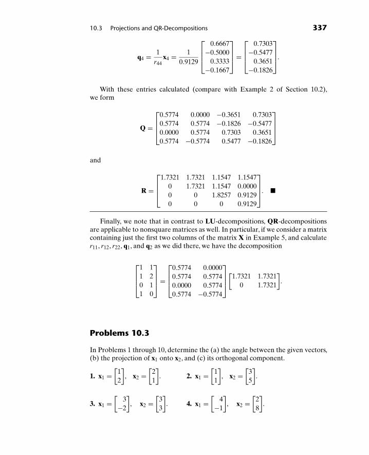
10.3 Projections and QR-Decompositions 337
q4 = 1r44
x4 = 10.9129
⎡⎢⎢⎣
0.6667−0.5000
0.3333−0.1667
⎤⎥⎥⎦ =
⎡⎢⎢⎣
0.7303−0.5477
0.3651−0.1826
⎤⎥⎥⎦.
With these entries calculated (compare with Example 2 of Section 10.2),we form
Q =
⎡⎢⎢⎣
0.5774 0.0000 −0.3651 0.73030.5774 0.5774 −0.1826 −0.54770.0000 0.5774 0.7303 0.36510.5774 −0.5774 0.5477 −0.1826
⎤⎥⎥⎦
and
R =
⎡⎢⎢⎣
1.7321 1.7321 1.1547 1.15470 1.7321 1.1547 0.00000 0 1.8257 0.91290 0 0 0.9129
⎤⎥⎥⎦. �
Finally, we note that in contrast to LU-decompositions, QR-decompositionsare applicable to nonsquare matrices as well. In particular, if we consider a matrixcontaining just the first two columns of the matrix X in Example 5, and calculater11, r12, r22, q1, and q2 as we did there, we have the decomposition
⎡⎢⎢⎣
1 11 20 11 0
⎤⎥⎥⎦ =
⎡⎢⎢⎣
0.5774 0.00000.5774 0.57740.0000 0.57740.5774 −0.5774
⎤⎥⎥⎦[
1.7321 1.73210 1.7321
].
Problems 10.3
In Problems 1 through 10, determine the (a) the angle between the given vectors,(b) the projection of x1 onto x2, and (c) its orthogonal component.
1. x1 =[
12
], x2 =
[21
]. 2. x1 =
[11
], x2 =
[35
].
3. x1 =[
3−2
], x2 =
[33
]. 4. x1 =
[4
−1
], x2 =
[28
].

338 Chapter 10 Real Inner Products and Least-Square
5. x1 =[−7−2
], x2 =
[29
]. 6. x1 =
⎡⎣2
10
⎤⎦, x2 =
⎡⎣2
02
⎤⎦.
7. x1 =⎡⎣1
10
⎤⎦, x2 =
⎡⎣2
21
⎤⎦. 8. x1 =
⎡⎣0
34
⎤⎦, x2 =
⎡⎣2
55
⎤⎦.
9. x1 =
⎡⎢⎢⎣
0111
⎤⎥⎥⎦, x2 =
⎡⎢⎢⎣
1110
⎤⎥⎥⎦. 10. x1 =
⎡⎢⎢⎣
1234
⎤⎥⎥⎦, x2 =
⎡⎢⎢⎣
1−2
0−1
⎤⎥⎥⎦.
In Problems 11 through 21, determine QR-decompositions for the given matrices.
11.[
1 22 1
]. 12.
[1 31 5
]. 13.
[3 3
−2 3
].
14.
⎡⎣1 2
2 22 1
⎤⎦. 15.
⎡⎣1 1
1 03 5
⎤⎦. 16.
⎡⎢⎢⎣
3 1−2 1
1 1−1 1
⎤⎥⎥⎦.
17.
⎡⎣2 0 2
1 1 00 1 2
⎤⎦. 18.
⎡⎣1 2 2
1 0 20 1 1
⎤⎦. 19.
⎡⎣0 3 2
3 5 54 0 5
⎤⎦.
20.
⎡⎢⎢⎣
0 1 11 0 11 1 01 1 1
⎤⎥⎥⎦. 21.
⎡⎢⎢⎣
1 0 11 1 00 −1 −10 0 0
⎤⎥⎥⎦.
22. Show that
∥∥∥∥ 〈x, a〉〈a, a〉a
∥∥∥∥ = ‖x‖|cos θ|,
where θ is the angle between x and a.
23. Prove directly that
x − 〈a, x〉〈a, a〉a
is orthogonal to a.
24. Discuss what is likely to occur in a QR-decomposition if the columns are notlinearly independent, and all calculations are rounded.

10.4 The QR-Algorithm 339
10.4 The QR-Algorithm
The QR-algorithm is one of the more powerful numerical methods developedfor computing eigenvalues of real matrices. In contrast to the power methodsdescribed in Section 6.6, which converge only to a single dominant real eigenvalueof a matrix, the QR-algorithm generally locates all eigenvalues, both real andcomplex, regardless of multiplicity.
Although a proof of the QR-algorithm is beyond the scope of this book, thealgorithm itself is deceptively simple. As its name suggests, the algorithm is basedon QR-decompositions. Not surprisingly then, the algorithm involves numerousarithmetic calculations, making it unattractive for hand computations but idealfor implementation on a computer.
Like many numerical methods, the QR-algorithm is iterative. We begin witha square real matrix A0. To determine its eigenvalues, we create a sequence ofnew matrices A1, A2, . . . , Ak−1, Ak, . . . , having the property that each new matrixhas the same eigenvalues as A0, and that these eigenvalues become increasinglyobvious as the sequence progresses. To calculate Ak (k = 1, 2, 3, . . .) once Ak−1 isknown, first construct a QR-decomposition of Ak−1:
Ak−1 = Qk−1Rk−1,
and then reverse the order fo the product to define
Ak = Rk−1Qk−1.
It can be shown that each matrix in the sequence {Ak} (k = 1, 2, 3, . . .) has identicaleigenvalues. For now, we just note that the sequence generally converges to oneof the following two partitioned forms:
[S --
-
T- - - - - - - - - - - - - - - - - - - - -0 0 0 · · · 0 --
-
a
](15)
or ⎡⎢⎣ U --
- V- - - - - - - - - - - - - - - - - - - - - - - -0 0 0 · · · 0 b c
0 0 0 · · · 0 ----
-
d e
⎤⎥⎦. (16)
If matrix (15) occurs, then the element a is an eigenvalue, and the remainingeigenvalues are found by applying the QR-algorithm a new to the submatrix S.If, on the other hand, matrix (16) occurs, then two eigenvalues are determined bysolving for the roots of the characteristic equation of the 2 × 2 matrix in the lowerright partition, namely
λ2 − (b + e)λ + (be − cd) = 0.

340 Chapter 10 Real Inner Products and Least-Square
The remaining eigenvalues are found by applying the QR-algorithm anew to thesubmatrix U.
Convergence of the algorithm is accelerated by performing a shift at eachiteration. If the orders of all matrices are n × n, we denote the element in the(n, n)-position of the matrix Ak−1 as wk−1,and construct a QR-decomposition forthe shifted matrix Ak−1 − wk−1I. That is,
Ak−1 − wk−1I = Qk−1Rk−1. (17)
We define
Ak = Rk−1Qk−1 + wk−1I. (18)
Example 1 Find the eigenvalues of
A0 =⎡⎣ 0 1 0
0 0 118 −1 −7
⎤⎦.
Solution Using the QR-algorithm with shifting, carrying all calculations to eightsignificant figures but rounding to four decimals for presentation, we compute
A0 − (−7)I =⎡⎣ 7 1 0
0 7 118 −1 0
⎤⎦
=⎡⎣0.3624 0.1695 −0.9165
0.0000 0.9833 0.18180.9320 −0.0659 0.3564
⎤⎦⎡⎣19.3132 −0.5696 0.0000
0.0000 7.1187 0.98330.0000 0.0000 0.1818
⎤⎦
= Q0R0,
A1 = R0Q0 + (−7)I
=⎡⎣19.3132 −0.5696 0.0000
0.0000 7.1187 0.98330.0000 0.0000 0.1818
⎤⎦⎡⎣0.3624 0.1695 −0.9165
0.0000 0.9833 0.18180.9320 −0.0659 0.3564
⎤⎦
+⎡⎣−7 0 0
0 −7 00 0 −7
⎤⎦
=⎡⎣0.0000 2.7130 −17.8035
0.9165 −0.0648 1.64490.1695 −0.0120 −6.9352
⎤⎦,

10.4 The QR-Algorithm 341
A1 − (−6.9352)I =⎡⎣6.9352 2.7130 −17.8035
0.9165 6.8704 1.64490.1695 −0.0120 0.0000
⎤⎦
=⎡⎣0.9911 −0.1306 −0.0260
0.1310 0.9913 0.01200.0242 −0.0153 0.9996
⎤⎦⎡⎣6.9975 3.5884 −17.4294
0.0000 6.4565 3.95620.0000 0.0000 0.4829
⎤⎦
= Q1R1,
A2 = R1Q1 + (−6.9352)I =⎡⎣0.0478 2.9101 −17.5612
0.9414 −0.5954 4.03220.0117 −0.0074 −6.4525
⎤⎦.
Continuing in this manner, we generate sequentially
A3 =⎡⎣0.5511 2.7835 −16.8072
0.7826 −1.1455 6.52000.0001 −0.0001 −6.4056
⎤⎦
and
A4 =⎡⎣0.9259 2.5510 −15.9729
0.5497 −1.5207 8.35830.0000 −0.0000 −6.4051
⎤⎦.
A4 has form (15) with
S =[
0.9259 2.55100.5497 −1.5207
]and a = −6.4051.
One eigenvalue is −6.4051, which is identical to the value obtained in Example 2of Section 6.6. In addition, the characteristic equation of R is λ2 + 0.5948λ −2.8103 = 0, which admits both −2 and 1.4052 as roots. These are the other twoeigenvalues of A0. �
Example 2 Find the eigenvalues of
A0 =
⎡⎢⎢⎣
0 0 0 −251 0 0 300 1 0 −180 0 1 6
⎤⎥⎥⎦.

342 Chapter 10 Real Inner Products and Least-Square
Solution Using the QR-algorithm with shifting, carrying all calculations to eightsignificant figures but rounding to four decimals for presentation, we compute
A0 − (6)I =
⎡⎢⎢⎣
−6 0 0 −251 −6 0 300 1 −6 −180 0 1 0
⎤⎥⎥⎦
=
⎡⎢⎢⎣
−0.9864 −0.1621 −0.0270 −0.00460.1644 −0.9726 −0.1620 −0.02740.0000 0.1666 −0.9722 −0.16430.0000 0.0000 0.1667 −0.9860
⎤⎥⎥⎦
×
⎡⎢⎢⎣
6.0828 −0.9864 0.0000 −29.59180.0000 6.0023 −0.9996 −28.12460.0000 0.0000 6.0001 13.31420.0000 0.0000 0.0000 2.2505
⎤⎥⎥⎦
= Q0R0,
A1 = R0Q0 + (6)I =
⎡⎢⎢⎣
−0.1622 −0.0266 4.9275 −29.17870.9868 −0.0044 −4.6881 27.73110.0000 0.9996 2.3856 −14.11400.0000 0.0000 0.3751 3.7810
⎤⎥⎥⎦,
A1 − (3.7810)I =
⎡⎢⎢⎣
−3.9432 −0.0266 4.9275 −29.17870.9868 −3.7854 −4.6881 27.73110.0000 0.9996 −1.3954 −14.11400.0000 0.0000 0.3751 0.0000
⎤⎥⎥⎦
=
⎡⎢⎢⎣
−0.9701 −0.2343 −0.0628 −0.01060.2428 −0.9361 −0.2509 −0.04230.0000 0.2622 −0.9516 −0.16040.0000 0.0000 0.1662 −0.9861
⎤⎥⎥⎦
×
⎡⎢⎢⎣
4.0647 −0.8931 −5.9182 35.03790.0000 3.8120 2.8684 −22.82570.0000 0.0000 2.2569 8.30600.0000 0.0000 0.0000 1.3998
⎤⎥⎥⎦
= Q1R1,
A2 = R1Q1 + (3.7810)I =
⎡⎢⎢⎣
−0.3790 −1.6681 11.4235 −33.60680.9254 0.9646 −7.4792 21.88710.0000 0.5918 3.0137 −8.55240.0000 0.0000 0.2326 2.4006
⎤⎥⎥⎦.

10.4 The QR-Algorithm 343
Continuing in this manner, we generate, after 25 iterations,
A25 =
⎡⎢⎢⎣
4.8641 −4.4404 18.1956 −28.76754.2635 −2.8641 13.3357 −21.33710.0000 0.0000 2.7641 −4.14380.0000 0.0000 0.3822 1.2359
⎤⎥⎥⎦,
which has form (16) with
U =[
4.8641 −4.44044.2635 −2.8641
]and
[b c
d e
]=[
2.7641 −4.14380.3822 1.2359
].
The characteristic equation of U is λ2 − 2λ + 5 = 0, which has as its roots 1 ± 2i;the characteristic equation of the other 2 × 2 matrix is λ2 − 4λ + 4.9999 = 0, whichhas as its roots 2 ± i. These roots are the four eigenvalues of A0. �
Problems 10.4
1. Use one iteration of the QR-algorithm to calculate A1 when
A0 =⎡⎣ 0 1 0
0 0 118 −1 7
⎤⎦.
Note that this matrix differs from the one in Example 1 by a single sign.
2. Use one iteration of the QR-algorithm to calculate A1 when
A0 =⎡⎣ 2 −17 7
−17 −4 17 1 −14
⎤⎦.
3. Use one iteration of the QR-algorithm to calculate A1 when
A0 =
⎡⎢⎢⎣
0 0 0 −131 0 0 40 1 0 −140 0 1 4
⎤⎥⎥⎦.
In Problems 4 through 14, use the QR-algorithm to calculate the eigenvaluesof the given matrices:
4. The matrix defined in Problem 1.
5. The matrix defined in Problem 2.

344 Chapter 10 Real Inner Products and Least-Square
6.
⎡⎣3 0 0
2 6 42 3 5
⎤⎦. 7.
⎡⎣7 2 0
2 1 60 6 7
⎤⎦. 8.
⎡⎣3 2 3
2 6 63 6 11
⎤⎦.
9.
⎡⎣ 2 0 −1
2 3 2−1 0 2
⎤⎦. 10.
⎡⎣1 1 0
0 1 15 −9 6
⎤⎦. 11.
⎡⎣ 3 0 5
1 1 1−2 0 −3
⎤⎦.
12. The matrix in Problem 3.
13.
⎡⎢⎢⎣
0 3 2 −11 0 2 −33 1 0 −12 −2 1 1
⎤⎥⎥⎦. 14.
⎡⎢⎢⎣
10 7 8 77 5 6 58 6 10 97 5 9 10
⎤⎥⎥⎦.
10.5 Least-Squares
Analyzing data for forecasting and predicting future events is common to business,engineering, and the sciences, both physical and social. If such data are plotted,as in Figure 10.4, they constitute a scatter diagram, which may provide insightinto the underlying relationship between system variables. For example, the datain Figure 10.4 appears to follow a straight line relationship reasonably well. Theproblem then is to determine the equation of the straight line that best fits the data.
A straight line in the variables x and y having the equation
y = mx + c, (19)
y
x
Figure 10.4

10.5 Least-Squares 345
y
x0 1 2 3 4
10
9
8
7
6
5
4
3
2
1
e(4)
e(3)
e(2)
e(1)
e(0)
y5
2x1
15
Denotes a data point
Denotes a point on thestraight line for the samey-value as the data point
Figure 10.5
where m and c are constants, will have one y-value on the line for each value ofx. This y-value may or may not agree with the data at the same value of x. Thus,for values of x at which data are available, we generally have two values of y, onevalue from the data and a second value from the straight line approximation tothe data. This situation is illustrated in Figure 10.5. The error at each x, designatedas e(x), is the difference between the y-value of the data and the y-value obtainedfrom the straight-line approximation.
Example 1 Calculate the errors made in approximating the data given inFigure 10.5 by the line y = 2x + 1.5.
Solution The line and the given data points are plotted in Figure 10.5. Thereare errors at x = 0, x = 1, x = 2, x = 3, and x = 4. Evaluating the equationy = 2x + 1.5 at these values of x, we compute Table 10.1.
It now follows that
e(0) = 1 − 1.5 = −0.5,
e(1) = 5 − 3.5 = 1.5,
e(2) = 3 − 5.5 = −2.5,
e(3) = 6 − 7.5 = −1.5,

346 Chapter 10 Real Inner Products and Least-Square
Table 10.1
Evaluated fromGiven data y = 2x + 1.5
x y y
0 1 1.51 5 3.52 3 5.53 6 7.54 9 9.5
and
e(4) = 9 − 9.5 = −0.5.
Note that these errors could have been read directly from the graph. �
We can extend this concept of error to the more general situation involving N datapoints. Let (x1, y1), (x2, y2), (x3, y3), . . . , (xN, yN) be a set of N data points for aparticular situation. Any straight-line approximation to this data generates errorse(x1), e(x2), e(x3), . . . , e(xN) which individually can be positive, negative, or zero.The latter case occurs when the approximation agrees with the data at a particularpoint. We define the overall error as follows.
Definition 1 The least-squares error E is the sum of the squares of the individualerrors. That is,
E = [e(x1)]2 + [e(x2)]2 + [e(x3)]2 + · · · + [e(xN)]2.
The only way the total error E can be zero is for each of the individual errors to bezero. Since each term of E is squared, an equal number of positive and negativeindividual errors cannot sum to zero.
Example 2 Compute the least-squares error for the approximation used inExample 1.
Solution
E = [e(0)]2 + [e(1)]2 + [e(2)]2 + [e(3)]2 + [e(4)]2
= (−0.5)2 + (1.5)2 + (−2.5)2 + (−1.5)2 + (−0.5)2
= 0.25 + 2.25 + 6.25 + 2.25 + 0.25
= 11.25. �

10.5 Least-Squares 347
Definition 2 The least-squares straight line is the line that minimizes theleast-squares error.
We seek values of m and c in (19) that minimize the least-squares error. Forsuch a line,
e(xi) = yi − (mxi + c),
so we want the values for m and c that minimize
E =N∑
i=1
(yi − mxi − c)2.
This occurs when
∂E
∂m=
N∑i=1
2(yi − mxi − c)(−xi) = 0
and
∂E
∂c=
N∑i=1
2(yi − mxi − c)(−1) = 0,
or, upon simplifying, when(N∑
i=1
x2i
)m +
(N∑
i=1
xi
)c =
N∑i=1
xiyi, (20)
(N∑
i=1
xi
)m + Nc =
N∑i=1
yi.
System (20) makes up the normal equations for a least-squares fit in twovariables.
Example 3 Find the least-squares straight line for the following x − y data:
x 0 1 2 3 4y 1 5 3 6 9
.
Solution Table 10.2 contains the required summations.
For this data, the normal equations become
30m + 10c = 65,
10m + 5c = 24,
which has as its solution m = 1.7 and c = 1.4. The least-squares straight line isy = 1.7x + 1.4.
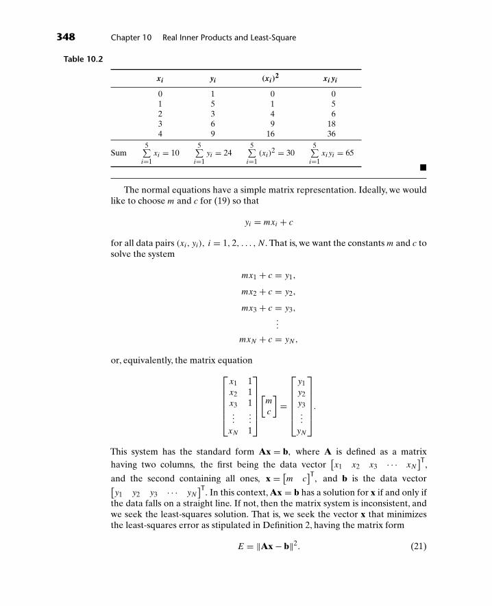
348 Chapter 10 Real Inner Products and Least-Square
Table 10.2
xi yi (xi)2 xiyi
0 1 0 01 5 1 52 3 4 63 6 9 184 9 16 36
Sum5∑
i=1xi = 10
5∑i=1
yi = 245∑
i=1(xi)
2 = 305∑
i=1xiyi = 65
�
The normal equations have a simple matrix representation. Ideally, we wouldlike to choose m and c for (19) so that
yi = mxi + c
for all data pairs (xi, yi), i = 1, 2, . . . , N. That is, we want the constants m and c tosolve the system
mx1 + c = y1,
mx2 + c = y2,
mx3 + c = y3,
...
mxN + c = yN,
or, equivalently, the matrix equation⎡⎢⎢⎢⎢⎢⎣
x1 1x2 1x3 1...
...
xN 1
⎤⎥⎥⎥⎥⎥⎦[m
c
]=
⎡⎢⎢⎢⎢⎢⎣
y1y2y3...
yN
⎤⎥⎥⎥⎥⎥⎦.
This system has the standard form Ax = b, where A is defined as a matrixhaving two columns, the first being the data vector
[x1 x2 x3 · · · xN
]T,
and the second containing all ones, x = [m c]T, and b is the data vector[
y1 y2 y3 · · · yN
]T. In this context, Ax = b has a solution for x if and only ifthe data falls on a straight line. If not, then the matrix system is inconsistent, andwe seek the least-squares solution. That is, we seek the vector x that minimizesthe least-squares error as stipulated in Definition 2, having the matrix form
E = ‖Ax − b‖2. (21)

10.5 Least-Squares 349
The solution is the vector x satisfying the normal equations, which take the matrixform
ATAx = ATb. (22)
System (22) is identical to system (20) when A and b are defined as above.We now generalize to all linear systems of the form Ax = b. We are primarily
interested in cases where the system is inconsistent (rendering the methods devel-oped in Chapter 2 useless), ands this generally occurs when A has more rows thancolumns. We shall place no restrictions on the number of columns in A, but wewill assume that the columns are linearly independent. We seek the vector x thatminimizes the least-squares error defined by Eq. (21).
Theorem 1 If x has the property that Ax − b is orthogonal to the columns of A,then x minimizes ‖Ax − b‖2.
Proof. For any vector x0 of appropriate dimension,
‖Ax0 − b‖2 = ‖(Ax0 − Ax) + (Ax − b)‖2
= 〈(Ax0 − Ax) + (Ax − b) , (Ax0 − Ax) + (Ax − b)〉= 〈(Ax0 − Ax) , (Ax0 − Ax)〉 + 〈(Ax − b) , (Ax − b)〉= +2 〈(Ax0 − Ax) , (Ax − b)〉= ‖(Ax0 − Ax)‖2 + ‖(Ax − b)‖2
= +2 〈Ax0, (Ax − b)〉 − 2 〈Ax, (Ax − b)〉 .
It follows directly from Problem 28 of Section 10.2 that the last two inner productsare both zero (take p = Ax − b). Therefore,
‖Ax0 − b‖2 = ‖(Ax0 − Ax)‖2 + ‖(Ax − b)‖2
≥ ‖(Ax − b)‖2,
and x minimizes Eq. (21).
As a consequence of Theorem 1, we seek a vector x having the propertythat Ax − b is orthogonal to the columns of A. Denoting the columns of A asA1, A2, . . . , An, respectively, we require
〈Ai, Ax − b〉 = 0 (i = 1, 2, . . . , n).
If y = [y1 y2 · · · yn
]T denotes an arbitrary vector of appropriate dimension,then
Ay = A1y1 + A2y2 + · · · + Anyn,

350 Chapter 10 Real Inner Products and Least-Square
and
〈Ay, (Ax − b)〉 =⟨
n∑i=1
Aiyi, (Ax − b)
⟩
=n∑
i=1
〈Aiyi, (Ax − b)〉 (23)
=n∑
i=1
yi 〈Ai, (Ax − b)〉
= 0.
It also follows from Problem 39 of Section 6.1 that
〈Ay, (Ax − b)〉 = 〈y, Aᵀ(Ax − b)〉 = 〈y, (AᵀAx − Aᵀb)〉. (24)
Eqs. (23) and (24) imply that 〈y, (AᵀAx − Aᵀb)〉 = 0 for any y. We may deducefrom Problem 26 of Section 10.2 that AᵀAx − Aᵀb = 0, or AᵀAx = Aᵀb, whichhas the same form as Eq. (22)! Therefore, a vector x is the least-squares solutionto Ax = b if and only if it is the solution to AᵀAx = Aᵀb. This set of normalequations is guaranteed to have a unique solution whenever the columns of A arelinearly independent, and it may be solved using any of the methods described inthe previous chapters!
Example 4 Find the least-squares solution to
x + 2y + z = 1,
3x − y = 2,
2x + y − z = 2,
x + 2y + 2z = 1.
Solution This system takes the matrix form Ax = b, with
A =
⎡⎢⎢⎣
1 2 13 −1 02 1 −11 2 2
⎤⎥⎥⎦, x =
⎡⎣x
y
z
⎤⎦, and b =
⎡⎢⎢⎣
1221
⎤⎥⎥⎦.
Then,
AᵀA =⎡⎣15 3 1
3 10 51 5 6
⎤⎦ and Aᵀb =
⎡⎣12
41
⎤⎦,

10.5 Least-Squares 351
and the normal equations become
⎡⎢⎣15 3 1
3 10 51 5 6
⎤⎥⎦
⎡⎢⎣x
y
z
⎤⎥⎦ =
⎡⎢⎣12
41
⎤⎥⎦.
Using Gaussian elimination, we obtain as the unique solution to this set of equa-tions x = 0.7597, y = 0.2607, and z = −0.1772, which is also the least-squaressolution to the original system. �
Example 5 Find the least-squares solution to
0x + 3y = 80,
2x + 5y = 100,
5x − 2y = 60,
−x + 8y = 130,
10x − y = 150.
Solution This system takes the matrix form Ax = b, with
A =
⎡⎢⎢⎢⎢⎢⎣
1 32 55 −2
−1 810 −1
⎤⎥⎥⎥⎥⎥⎦, x =
[x
y
], and b =
⎡⎢⎢⎢⎢⎢⎣
80100
60130150
⎤⎥⎥⎥⎥⎥⎦.
Then,
AᵀA =[
131 −15−15 103
]and Aᵀb =
[19501510
],
and the normal equations become
[131 −15−15 103
][x
y
]=[
19501510
].
The unique solution to this set of equations is x = 16.8450, and y = 17.1134,rounded to four decimals, which is also the least-squares solution to the originalsystem. �

352 Chapter 10 Real Inner Products and Least-Square
Problems 10.5
In Problems 1 through 8, find the least-squares solution to the given systems ofequations:
1. 2x + 3y = 8,
3x − y = 5,
x + y = 6.
2. 2x + y = 8,
x + y = 4,
−x + y = 0,
3x + y = 13.
3. x + 3y = 65,
2x − y = 0,
3x + y = 50,
2x + 2y = 55.
4. 2x + y = 6,
x + y = 8,
−2x + y = 11,
−x + y = 8,
3x + y = 4.
5. 2x + 3y − 4z = 1,
x − 2y + 3z = 3,
x + 4y + 2z = 6,
2x + y − 3z = 1.
6. 2x + 3y + 2z = 25,
2x − y + 3z = 30,
3x + 4y − 2z = 20,
3x + 5y + 4z = 55.
7. x + y − z = 90,
2x + y + z = 200,
x + 2y + 2z = 320,
3x − 2y − 4z = 10,
3x + 2y − 3z = 220.
8. x + 2y + 2z = 1,
2x + 3y + 2z = 2,
2x + 4y + 4z = −2,
3x + 5y + 4z = 1,
x + 3y + 2z = −1.
9. Which of the systems, if any, given in Problems 1 through 8 represent a least-squares, straight line fit to data?
10. The monthly sales figures (in thousands of dollars) for a newly opened shoestore are:
month 1 2 3 4 5
sales 9 16 14 15 21
(a) Plot a scatter diagram for this data.
(b) Find the least-squares straight line that best fits this data.
(c) Use this line to predict sales revenue for month 6.
11. The number of new cars sold at a new car dealership over the first 8 weeks ofthe new season are:
week 1 2 3 4 5 6 7 8
sales 51 50 45 46 43 39 35 34

10.5 Least-Squares 353
(a) Plot a scatter diagram for this data.
(b) Find the least-squares straight line that best fits this data.
(c) Use this line to predict sales for weeks 9 and 10.
12. Annual rainfall data (in inches) for a given town over the last seven years are:
year 1 2 3 4 5 6 7
rainfall 10.5 10.8 10.9 11.7 11.4 11.8 12.2
(a) Find the least-squares straight line that best fits this data.
(b) Use this line to predict next year’s rainfall.
13. Solve system (20) algebraically and explain why the solution would besusceptible to round-off error.
14. (Coding) To minimize the round-off error associated with solving the normalequations for a least-squares straight line fit, the (xi, yi)-data are coded beforeusing them in calculations. Each xi-value is replaced by the difference betweenxi and the average of all xi-data. That is, if
X = 1N
N∑i=1
xi, then set x′i = xi − X,
and fit a straight line to the (x′i, yi)-data instead.
Explain why this coding scheme avoids the round-off errors associatedwith uncoded data.
15. (a) Code the data given in Problem 10 using the procedure described inProblem 14.
(b) Find the least-squares straight line fit for this coded data.
16. (a) Code the data given in Problem 11 using the procedure described inProblem 14.
(b) Find the least-squares straight line fit for this coded data.
17. Census figures for the population (in millions of people) for a particular regionof the country are as follows:
year 1950 1960 1970 1980 1990
population 25.3 23.5 20.6 18.7 17.8
(a) Code this data using the procedure described in Problem 14, and thenfind the least-squares straight line that best fits it.
(b) Use this line to predict the population in 2000.

354 Chapter 10 Real Inner Products and Least-Square
18. Show that if A = QR is a QR-decomposition of A, then the normal equationsgiven by Eq. (22) can be written as RᵀRx = RᵀQᵀb, which reduces toRx = Qᵀb. This is a numerically stable set of equations to solve, not subjectto the same round-off errors associated with solving the normal equationsdirectly.
19. Use the procedure described in Problem 18 to solve Problem 1.
20. Use the procedure described in Problem 18 to solve Problem 2.
21. Use the procedure described in Problem 18 to solve Problem 5.
22. Use the procedure described in Problem 18 to solve Problem 6.
23. Determine the error vector associated with the least-squares solution ofProblem 1, and then calculate the inner product of this vector with each of thecolumns of the coefficient matrix associated with the given set of equations.
24. Determine the error vector associated with the least-squares solution ofProblem 5, and then calculate the inner product of this vector with each of thecolumns of the coefficient matrix associated with the given set of equations.

Appendix: A Word onTechnology
We have covered a number of topics which relied very heavily on computations.For example, in Chapter 6, we computed eigenvalues and in Chapter 9 we raisedtransitional matrices to certain powers.
While it is true that much of the “number crunching” involved the basic oper-ations of addition and multiplication, all would agree that much time could beconsumed with these tasks.
We, as educators, are firm believers that students of mathematics, science, andengineering should first understand the underlying fundamental concepts involvedwith the topics presented in this text. However, once these ideas are mastered,a common sense approach would be appropriate regarding laborious numericalcalculations.
As the first decade of this new millennium is coming to a close, we can takeadvantage of many tools. Calculators and Computer Algebra Systems are idealinstruments which can be employed.
We give a few suggestions below:
● TI-89 calculator produced by Texas Instruments (http://www.ti.com/)
● Various products developed by Maplesoft (http://www.maplesoft.com/)
● Various Mathematica ® software packages (http://www.wolfram.com/)
Thank you for using our text.
355

This page intentionally left blank

Answers and Hints to SelectedProblems
CHAPTER 1
Section 1.1
1. A is 4 × 5, B is 3 × 3, C is 3 × 4,
D is 4 × 4, E is 2 × 3, F is 5 × 1,
G is 4 × 2, H is 2 × 2, J is 1 × 3.
2. a13 = −2, a21 = 2,
b13 = 3, b21 = 0,
c13 = 3, c21 = 5,
d13 = t2, d21 = t − 2,
e13 = 14 , e21 = 2
3 ,
f13 = does not exist, f21 = 5,
g13 = does not exist, g21 = 2π,
h13 = does not exist, h21 = 0,
j13 = −30, j21 does not exist.
3. a23 = −6, a32 = 3, b31 = 4,
b32 = 3, c11 = 1, d = 22 t4, e13 = 14 ,
g22 = 18, g23 and h32 do not exist.
4. A =[
1 −1−1 1
]. 5. A =
⎡⎢⎢⎣
1 12
13
2 1 23
3 32 1
⎤⎥⎥⎦. 6. B =
⎡⎣ 1 0 −1
0 −1 −2−1 −2 −3
⎤⎦.
7. C =[
1 1 1 11 2 3 4
]. 8. D =
⎡⎣0 −1 −2 −3
3 0 −1 −24 5 0 −1
⎤⎦.
357

358 Answers and Hints to Selected Problems
9. (a)[9 15
], (b)
[12 0
], (c)
[13 30
], (d)
[21 15
].
10. (a)[7 4 1776
], (b)
[12 7 1941
], (c)
[4 23 1809
],
(d)[10 31 1688
].
11.[950 1253 98
]. 12.
⎡⎣3 5 3 4
0 2 9 54 2 0 0
⎤⎦. 13.
⎡⎣72 12 16
45 32 1681 10 35
⎤⎦.
14.
⎡⎣100 150 50 500
27 45 116 229 41 116 3
⎤⎦.
15. (a)[
1000 2000 30000.07 0.075 0.0725
]. (b)
[1070.00 2150.00 3217.50
0.075 0.08 0.0775
].
16.[
0.95 0.050.01 0.99
]. 17.
[0.6 0.40.7 0.3
]. 18.
⎡⎣0.10 0.50 0.40
0.20 0.60 0.200.25 0.65 0.10
⎤⎦.
19.
⎡⎣0.80 0.15 0.05
0.10 0.88 0.020.25 0.30 0.45
⎤⎦.
Section 1.2
1.[
2 46 8
]. 2.
[ −5 −10−15 −20
]. 3.
⎡⎢⎢⎣
9 3−3 6
9 −66 18
⎤⎥⎥⎦. 4.
⎡⎢⎢⎣
−20 200 −20
50 −3050 10
⎤⎥⎥⎦.
5.
⎡⎢⎢⎣
0 −11 00 0
−2 −2
⎤⎥⎥⎦. 6.
[6 8
10 12
]. 7.
[0 26 1
]. 8.
⎡⎢⎢⎣
1 3−1 0
8 −57 7
⎤⎥⎥⎦.
9.
⎡⎢⎢⎣
3 2−2 2
3 −24 8
⎤⎥⎥⎦. 10. Does not exist. 11.
[−4 −4−4 −4
]. 12.
[−2 −20 −7
].
13.
⎡⎢⎢⎣
5 −1−1 4−2 1−3 5
⎤⎥⎥⎦. 14.
⎡⎢⎢⎣
3 00 23 −20 4
⎤⎥⎥⎦. 15.
[17 2227 32
]. 16.
[5 63 18
].
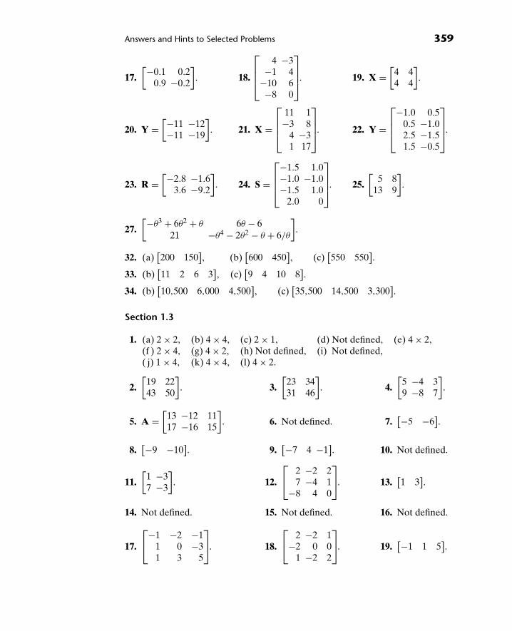
Answers and Hints to Selected Problems 359
17.[−0.1 0.2
0.9 −0.2
]. 18.
⎡⎢⎢⎣
4 −3−1 4
−10 6−8 0
⎤⎥⎥⎦. 19. X =
[4 44 4
].
20. Y =[−11 −12−11 −19
]. 21. X =
⎡⎢⎢⎣
11 1−3 8
4 −31 17
⎤⎥⎥⎦. 22. Y =
⎡⎢⎢⎣
−1.0 0.50.5 −1.02.5 −1.51.5 −0.5
⎤⎥⎥⎦.
23. R =[−2.8 −1.6
3.6 −9.2
]. 24. S =
⎡⎢⎢⎣
−1.5 1.0−1.0 −1.0−1.5 1.0
2.0 0
⎤⎥⎥⎦. 25.
[5 8
13 9
].
27.[−θ3 + 6θ2 + θ 6θ − 6
21 −θ4 − 2θ2 − θ + 6/θ
].
32. (a)[200 150
], (b)
[600 450
], (c)
[550 550
].
33. (b)[11 2 6 3
], (c)
[9 4 10 8
].
34. (b)[10,500 6,000 4,500
], (c)
[35,500 14,500 3,300
].
Section 1.3
1. (a) 2 × 2, (b) 4 × 4, (c) 2 × 1, (d) Not defined, (e) 4 × 2,(f ) 2 × 4, (g) 4 × 2, (h) Not defined, (i) Not defined,( j) 1 × 4, (k) 4 × 4, (l) 4 × 2.
2.[
19 2243 50
]. 3.
[23 3431 46
]. 4.
[5 −4 39 −8 7
].
5. A =[
13 −12 1117 −16 15
]. 6. Not defined. 7.
[−5 −6].
8.[−9 −10
]. 9.
[−7 4 −1]. 10. Not defined.
11.[
1 −37 −3
]. 12.
⎡⎣ 2 −2 2
7 −4 1−8 4 0
⎤⎦. 13.
[1 3
].
14. Not defined. 15. Not defined. 16. Not defined.
17.
⎡⎣−1 −2 −1
1 0 −31 3 5
⎤⎦. 18.
⎡⎣ 2 −2 1
−2 0 01 −2 2
⎤⎦. 19.
[−1 1 5].

360 Answers and Hints to Selected Problems
22.[
x + 2y
3x + 4y
]. 23.
⎡⎣ x − z
3x + y + z
x + 3y
⎤⎦. 24.
[a11x + a12y
a21x + a22y
].
25.[
2b11 − b12 + 3b132b21 − b22 + 3b23
]. 26.
[0 00 0
]. 27.
[0 40
−16 8
].
28.
⎡⎣0 0 0
0 0 00 0 0
⎤⎦. 29.
[7 5
11 10
]. 32.
[2 34 −5
][x
y
]=[
1011
].
33.
⎡⎣1 1 1
2 1 31 1 0
⎤⎦⎡⎣x
y
z
⎤⎦ =
⎡⎣2
40
⎤⎦. 34.
⎡⎢⎢⎣
5 3 2 41 1 0 13 2 2 01 1 2 3
⎤⎥⎥⎦⎡⎢⎢⎣
x
y
z
w
⎤⎥⎥⎦ =
⎡⎢⎢⎣
50
−34
⎤⎥⎥⎦.
35. (a) PN = [38,000], which represents the total revenue for that flight.
(b) NP =⎡⎣26,000 45,5000 65,000
4,000 7,000 10,0002,000 3,500 5,000
⎤⎦,
which has no physical significance.
36. (a) HP = [9,625 9,762.50 9,887.50 10,100 9,887.50], which representsthe portfolio value each day.
(b) PH does not exist.
37. TW = [14.00 65.625 66.50]T, which denotes the cost of producing eachproduct.
38. OTW = [33,862.50], which denotes the cost of producing all items on order.
39. FC =⎡⎣ 613 625
887 9601870 1915
⎤⎦,
which represents the number of each sex in each state of sickness.
Section 1.4
1.
⎡⎣7 4 −1
6 1 02 2 −6
⎤⎦. 2.
⎡⎢⎢⎣
t3 + 3t 2t2 + 3 32t3 + t2 4t2 + t t
t4 + t2 + t 2t3 + t + 1 t + 1t5 2t4 0
⎤⎥⎥⎦.
3. (a) BAT, (b) 2AT + B, (c) (BT + C)A = BTA + CA, (d) AB + CT,
(e) ATAT + ATA − AAT − AA.
4. XTX = [29], and XXT =⎡⎣4 6 8
6 9 128 12 16
⎤⎦.

Answers and Hints to Selected Problems 361
5. XTX =
⎡⎢⎢⎣
1 −2 3 −4−2 4 −6 8
3 −6 9 −12−4 8 −12 16
⎤⎥⎥⎦, and XXT = [30].
6.[2x2 + 6xy + 4y2]. 7. A, B, D, F, M, N, R, and T.
8. E, F, H, K, L, M, N, R, and T. 9. Yes.
10. No, see H and L in Problem 7. 11. Yes, see L in Problem 7.
12.
⎡⎣−5 0 0
0 9 00 0 2
⎤⎦. 14. No.
19. D2 is a diagonal matrix with diagonal elements 4, 9, and 25; D3 is a diagonalmatrix with diagonal elements 8, 27, and −125.
20. A diagonal matrix with diagonal elements 1, 8, 27.
23. A diagonal matrix with diagonal elements 4, 0, 10. 25. 4.
28. A = B + C. 29.
⎡⎢⎢⎢⎣
1 72 − 1
2
72 1 5
− 12 5 −8
⎤⎥⎥⎥⎦+
⎡⎢⎢⎢⎣
0 32 − 1
2
− 32 0 −2
12 2 0
⎤⎥⎥⎥⎦.
30.
⎡⎢⎢⎣
6 32 1
32 0 −4
1 −4 2
⎤⎥⎥⎦+
⎡⎢⎢⎣
0 − 12 2
12 0 3
−2 −3 0
⎤⎥⎥⎦.
34. (a) P2 =[
0.37 0.630.28 0.72
]and P3 =
[0.289 0.7110.316 0.684
],
(b) 0.37, (c) 0.63, (d) 0.711, (e) 0.684.
35. 1 → 1 → 1 → 1, 1 → 1 → 2 → 1, 1 → 2 → 1 → 1, 1 → 2 → 2 → 1.
36. (a) 0.097, (b) 0.0194. 37. (a) 0.64, (b) 0.636.
38. (a) 0.1, (b) 0.21. 39. (a) 0.6675, (b) 0.577075, (c) 0.267.
40. M =
⎡⎢⎢⎢⎢⎢⎢⎢⎢⎣
0 1 0 0 0 0 01 0 0 0 0 1 00 0 0 1 1 0 00 0 1 0 0 1 00 0 1 0 0 1 10 1 0 1 1 0 00 0 0 0 1 0 1
⎤⎥⎥⎥⎥⎥⎥⎥⎥⎦
.

362 Answers and Hints to Selected Problems
41. (a) M =
⎡⎢⎢⎢⎢⎣
0 2 0 1 02 0 0 2 10 0 0 1 01 2 1 0 10 1 0 1 0
⎤⎥⎥⎥⎥⎦,
(b) 3 paths consisting of 2 arcs connecting node 1 to node 5.
42. (a) M =
⎡⎢⎢⎢⎢⎢⎢⎢⎢⎢⎢⎣
0 1 1 0 1 0 0 01 0 1 0 1 0 0 01 1 0 0 1 0 0 00 0 0 0 1 1 1 01 1 1 1 0 1 0 00 0 0 1 1 0 0 10 0 0 1 0 0 0 10 0 0 0 0 1 1 0
⎤⎥⎥⎥⎥⎥⎥⎥⎥⎥⎥⎦
,
(b) M3 has a path from node 1 to node 7; it is the first integral power of Mhaving m17 positive. The minimum number of intermediate cities is two.
Section 1.5
1. (a), (b), and (d) are submatrices. 3.
⎡⎣ 4 5 −1 9
15 10 4 221 1 5 9
⎤⎦.
4. Partition A and B into four 2 × 2 submatrices each. Then,
AB =
⎡⎢⎢⎣
11 9 0 04 6 0 00 0 2 10 0 4 −1
⎤⎥⎥⎦.
5.
⎡⎢⎢⎣
18 6 0 012 6 0 0
0 0 1 00 0 3 4
⎤⎥⎥⎦. 6.
⎡⎢⎢⎣
7 8 0 0−4 −1 0 0
0 0 5 10 0 1 2
⎤⎥⎥⎦.
7. A2 =
⎡⎢⎢⎢⎢⎢⎢⎣
1 0 0 0 0 00 4 0 0 0 00 0 0 0 1 00 0 0 0 0 10 0 0 0 0 00 0 0 0 0 0
⎤⎥⎥⎥⎥⎥⎥⎦. A3 =
⎡⎢⎢⎢⎢⎢⎢⎣
1 0 0 0 0 00 8 0 0 0 00 0 0 0 0 10 0 0 0 0 00 0 0 0 0 00 0 0 0 0 0
⎤⎥⎥⎥⎥⎥⎥⎦.
8. An = A when n is odd.

Answers and Hints to Selected Problems 363
Section 1.6
1. p = 1. 2.
⎡⎢⎢⎣
−4/3−1−8/3
1/3
⎤⎥⎥⎦. 3.
[1 −0.4 1
].
4. (a) Not defined, (b)
⎡⎢⎢⎣
6 −3 12 32 −1 4 1
12 −6 24 60 0 0 0
⎤⎥⎥⎦, (c) [29], (d) [29].
5. (a)[4 −1 1
], (b) [−1], (c)
⎡⎣ 2 0 −2
−1 0 13 0 −3
⎤⎦, (d)
⎡⎣ 1 0 −1
0 0 0−1 0 1
⎤⎦.
6. (c), (d), (f), (g), (h), and (i).
7. (a)√
2, (b) 5, (c)√
3, (d) 12
√3, (e)
√15, (f)
√39.
8. (a)√
2, (b)√
5, (c)√
3, (d) 2, (e)√
30, (f)√
2.
9. (a)√
15, (b)√
39. 12. x
[24
]+ y
[35
]=[
1011
].
13. x
⎡⎣ 3
0−1
⎤⎦+ y
⎡⎣4
11
⎤⎦+ z
⎡⎣ 5
−22
⎤⎦+ w
⎡⎣ 6
8−1
⎤⎦ =
⎡⎣1
00
⎤⎦. 16.
[0.5 0.3 0.2
].
17. (a) There is a 0.6 probability that an individual chosen at random initially willlive in the city; thus, 60% of the population initially lives in the city, while40% lives in the suburbs.
(b) d(1) = [0.574 0.426]. (c) d(2) = [0.54956 0.45044].18. (a) 40% of customers now use brand X, 50% use brand Y, and 10% use other
brands.
(b) d1 = [0.395 0.530 0.075]. (c) d2 = [0.38775 0.54815 0.06410].19. (a) d(0) = [0 1]. (b) d(1) = [0.7 0.3].
20. (a) d(0) = [1 0 0].(b) d(2) = [0.21 0.61 0.18]. A probability of 0.18 that the harvest will be good
in two years.

364 Answers and Hints to Selected Problems
Section 1.7
1.
4.

Answers and Hints to Selected Problems 365
6.
7.

366 Answers and Hints to Selected Problems
16.
17. 341.57◦. 18. 111.80◦. 19. 225◦. 20. 59.04◦. 21. 270◦.
CHAPTER 2
Section 2.1
1. (a) No. (b) Yes. 2. (a) Yes. (b) No. (c) Yes.
3. No value of k will work. 4. k = 1. 5. k = 1/12.
6. k is arbitrary; any value will work. 7. No value of k will work.
8.[
3 52 −7
][x
y
]=[
11−3
]. 9.
⎡⎣1 1 2
1 −1 −21 2 2
⎤⎦⎡⎣x
y
z
⎤⎦ =
⎡⎣2
01
⎤⎦.
10.
⎡⎣1 2 3
1 −3 23 −4 7
⎤⎦⎡⎣x
y
z
⎤⎦ =
⎡⎣6
06
⎤⎦. 11.
⎡⎣ 1 2 2
2 4 2−3 −6 −4
⎤⎦⎡⎣x
y
z
⎤⎦ =
⎡⎣0
00
⎤⎦.
12. 50r + 60s = 70,000,
30r + 40s = 45,000.
13. 5d + 0.25b = 200,
10d + b = 500.
14. 8,000A + 3,000B + 1,000C = 70,000,
5,000A + 12,000B + 10,000C = 181,000,
1,000A + 3,000B + 2,000C = 41,000.
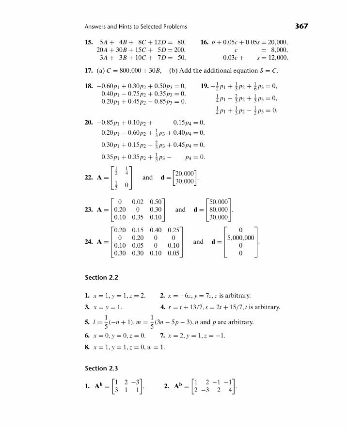
Answers and Hints to Selected Problems 367
15. 5A + 4B + 8C + 12D = 80,
20A + 30B + 15C + 5D = 200,
3A + 3B + 10C + 7D = 50.
16. b + 0.05c + 0.05s = 20,000,
c = 8,000,
0.03c + s = 12,000.
17. (a) C = 800,000 + 30B, (b) Add the additional equation S = C.
18. −0.60p1 + 0.30p2 + 0.50p3 = 0,
0.40p1 − 0.75p2 + 0.35p3 = 0,
0.20p1 + 0.45p2 − 0.85p3 = 0.
19. − 12p1 + 1
3p2 + 16p3 = 0,
14p1 − 2
3p2 + 13p3 = 0,
14p1 + 1
3p2 − 12p3 = 0.
20. −0.85p1 + 0.10p2 + 0.15p4 = 0,
0.20p1 − 0.60p2 + 13p3 + 0.40p4 = 0,
0.30p1 + 0.15p2 − 23p3 + 0.45p4 = 0,
0.35p1 + 0.35p2 + 13p3 − p4 = 0.
22. A =⎡⎣ 1
214
13 0
⎤⎦ and d =
[20,00030,000
].
23. A =⎡⎣ 0 0.02 0.50
0.20 0 0.300.10 0.35 0.10
⎤⎦ and d =
⎡⎣50,000
80,00030,000
⎤⎦.
24. A =
⎡⎢⎢⎣
0.20 0.15 0.40 0.250 0.20 0 0
0.10 0.05 0 0.100.30 0.30 0.10 0.05
⎤⎥⎥⎦ and d =
⎡⎢⎢⎣
05,000,000
00
⎤⎥⎥⎦.
Section 2.2
1. x = 1, y = 1, z = 2. 2. x = −6z, y = 7z, z is arbitrary.
3. x = y = 1. 4. r = t + 13/7, s = 2t + 15/7, t is arbitrary.
5. l = 15(−n + 1), m = 1
5(3n − 5p − 3), n and p are arbitrary.
6. x = 0, y = 0, z = 0. 7. x = 2, y = 1, z = −1.
8. x = 1, y = 1, z = 0, w = 1.
Section 2.3
1. Ab =[
1 2 −33 1 1
]. 2. Ab =
[1 2 −1 −12 −3 2 4
].

368 Answers and Hints to Selected Problems
3. Ab =⎡⎣ 1 2 5
−3 1 134 3 0
⎤⎦. 4. Ab =
⎡⎣2 4 0 2
3 2 1 85 −3 7 15
⎤⎦.
5. Ab =⎡⎣2 3 −4 12
3 −2 0 −18 −1 −4 10
⎤⎦. 6. x + 2y = 5,
y = 8.
7. x − 2y + 3z = 10,
y − 5z = −3,
z = 4.
8. r − 3s + 12t = 40,
s − 6t = −200,
t = 25.
9. x + 3y = −8,
y + 4z = 2,
0 = 0.
10. a − 7b + 2c = 0,
b − c = 0,
0 = 0.
11. u − v = −1,
v − 2w = 2,
w = −3,
0 = 1.
12. x = −11, y = 8. 13. x = 32, y = 17, z = 4.
14. r = −410, s = −50, t = 25.
15. x = −14 + 12z, y = 2 − 4z, z is arbitrary.
16. a = 5c, b = c, c is arbitrary.
17. No solution.
18.[
1 −2 50 1 23
]. 19.
[1 6 50 1 18
]. 20.
[1 3.5 −2.50 1 −6
].
21.
⎡⎣1 2 3 4
0 1 5 70 0 1 41/29
⎤⎦. 22.
⎡⎣1 3 2 1
0 1 −2 40 0 1 −32/23
⎤⎦.
23.
⎡⎢⎢⎣
1 3 2 00 1 −5 10 0 1 −9/350 0 0 0
⎤⎥⎥⎦. 24.
⎡⎣1 3/2 2 3 0 5
0 1 −50 −32 −6 −1300 0 1 53/76 5/76 190/76
⎤⎦.
25. x = 1, y = −2.
26. x = 5/7 − (1/7)z, y = −6/7 + (4/7)z, z is arbitrary.
27. a = −3, b = 4. 28. r = 13/3, s = t = −5/3.
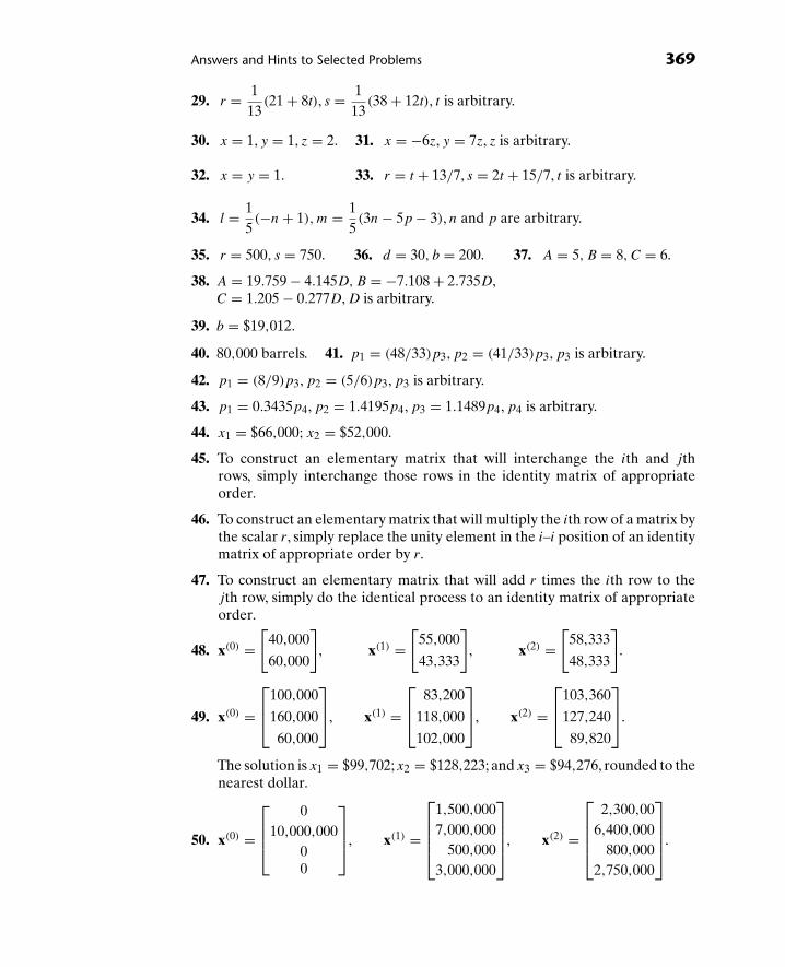
Answers and Hints to Selected Problems 369
29. r = 113
(21 + 8t), s = 113
(38 + 12t), t is arbitrary.
30. x = 1, y = 1, z = 2. 31. x = −6z, y = 7z, z is arbitrary.
32. x = y = 1. 33. r = t + 13/7, s = 2t + 15/7, t is arbitrary.
34. l = 15(−n + 1), m = 1
5(3n − 5p − 3), n and p are arbitrary.
35. r = 500, s = 750. 36. d = 30, b = 200. 37. A = 5, B = 8, C = 6.
38. A = 19.759 − 4.145D, B = −7.108 + 2.735D,C = 1.205 − 0.277D, D is arbitrary.
39. b = $19,012.
40. 80,000 barrels. 41. p1 = (48/33)p3, p2 = (41/33)p3, p3 is arbitrary.
42. p1 = (8/9)p3, p2 = (5/6)p3, p3 is arbitrary.
43. p1 = 0.3435p4, p2 = 1.4195p4, p3 = 1.1489p4, p4 is arbitrary.
44. x1 = $66,000; x2 = $52,000.
45. To construct an elementary matrix that will interchange the ith and jthrows, simply interchange those rows in the identity matrix of appropriateorder.
46. To construct an elementary matrix that will multiply the ith row of a matrix bythe scalar r, simply replace the unity element in the i–i position of an identitymatrix of appropriate order by r.
47. To construct an elementary matrix that will add r times the ith row to thejth row, simply do the identical process to an identity matrix of appropriateorder.
48. x(0) =[
40,000
60,000
], x(1) =
[55,000
43,333
], x(2) =
[58,333
48,333
].
49. x(0) =⎡⎢⎣100,000
160,000
60,000
⎤⎥⎦, x(1) =
⎡⎢⎣ 83,200
118,000
102,000
⎤⎥⎦, x(2) =
⎡⎢⎣103,360
127,240
89,820
⎤⎥⎦.
The solution is x1 = $99,702; x2 = $128,223; and x3 = $94,276, rounded to thenearest dollar.
50. x(0) =
⎡⎢⎢⎣
010,000,000
00
⎤⎥⎥⎦, x(1) =
⎡⎢⎢⎢⎣
1,500,0007,000,000
500,0003,000,000
⎤⎥⎥⎥⎦, x(2) =
⎡⎢⎢⎢⎣
2,300,006,400,000
800,0002,750,000
⎤⎥⎥⎥⎦.
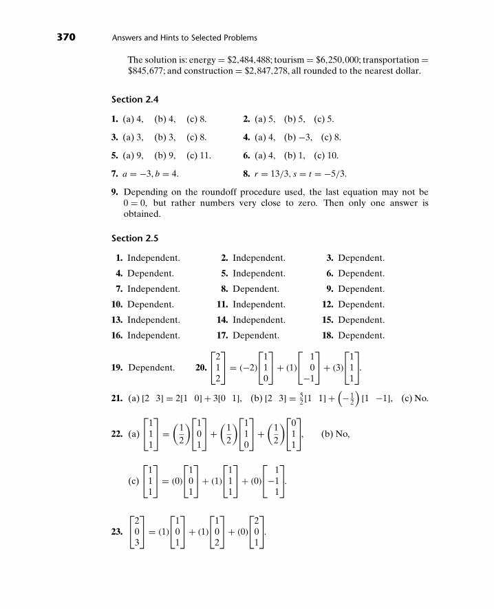
370 Answers and Hints to Selected Problems
The solution is: energy = $2,484,488; tourism = $6,250,000; transportation =$845,677; and construction = $2,847,278, all rounded to the nearest dollar.
Section 2.4
1. (a) 4, (b) 4, (c) 8. 2. (a) 5, (b) 5, (c) 5.
3. (a) 3, (b) 3, (c) 8. 4. (a) 4, (b) −3, (c) 8.
5. (a) 9, (b) 9, (c) 11. 6. (a) 4, (b) 1, (c) 10.
7. a = −3, b = 4. 8. r = 13/3, s = t = −5/3.
9. Depending on the roundoff procedure used, the last equation may not be0 = 0, but rather numbers very close to zero. Then only one answer isobtained.
Section 2.5
1. Independent. 2. Independent. 3. Dependent.
4. Dependent. 5. Independent. 6. Dependent.
7. Independent. 8. Dependent. 9. Dependent.
10. Dependent. 11. Independent. 12. Dependent.
13. Independent. 14. Independent. 15. Dependent.
16. Independent. 17. Dependent. 18. Dependent.
19. Dependent. 20.
⎡⎣2
12
⎤⎦ = (−2)
⎡⎣1
10
⎤⎦+ (1)
⎡⎣ 1
0−1
⎤⎦+ (3)
⎡⎣1
11
⎤⎦.
21. (a) [2 3] = 2[1 0] + 3[0 1], (b) [2 3] = 52 [1 1] +
(− 1
2
)[1 −1], (c) No.
22. (a)
⎡⎣1
11
⎤⎦ =
(12
)⎡⎣101
⎤⎦+
(12
)⎡⎣110
⎤⎦+
(12
)⎡⎣011
⎤⎦, (b) No,
(c)
⎡⎣1
11
⎤⎦ = (0)
⎡⎣1
01
⎤⎦+ (1)
⎡⎣1
11
⎤⎦+ (0)
⎡⎣ 1
−11
⎤⎦.
23.
⎡⎣2
03
⎤⎦ = (1)
⎡⎣1
01
⎤⎦+ (1)
⎡⎣1
02
⎤⎦+ (0)
⎡⎣2
01
⎤⎦.

Answers and Hints to Selected Problems 371
24. [a b] = (a)[1 0] + (b)[0 1].
25. [a b] =(
a + b
2
)[1 1] +
(a − b
2
)[1 −1].
26. [1 0] cannot be written as a linear combination of these vectors.
27. [a −2a] = (a/2)[2 −4] + (0)[−3 6].
28. [a b] =(
a + 2b
7
)[1 3] +
(3a − b
7
)[2 −1] + (0)[1 1].
29.
⎡⎣a
b
c
⎤⎦ =
(a − b + c
2
)⎡⎣101
⎤⎦+
(a + b − c
2
)⎡⎣110
⎤⎦+
(−a + b + c
2
)⎡⎣011
⎤⎦.
30. No, impossible to write any vector with a nonzero second component as alinear combination of these vectors.
31.
⎡⎣a
0a
⎤⎦ = (a)
⎡⎣1
01
⎤⎦+ (0)
⎡⎣1
02
⎤⎦+ (0)
⎡⎣2
01
⎤⎦. 32. 1 and 2 are bases.
33. 7 and 11 are bases. 39. (−k)x + (1)kx = 0.
42. 0 = A0 = A(c1x1 + c2x2 + · · · + ckxk) = c1Ax1 + c2Ax2 + · · · + ckAxk
= c1y1 + c2y2 + · · · + ckyk
).
Section 2.6
1. 2. 2. 2. 3. 1. 4. 2. 5. 3.
6. Independent. 7. Independent. 8. Dependent.
9. Dependent. 10. Independent. 11. Dependent.
12. Independent. 13. Dependent. 14. Dependent.
15. Dependent. 16. Independent. 17. Dependent.
18. Independent. 19. Dependent. 20. Independent.
21. Dependent. 22. Dependent.
23. (a) Yes, (b) Yes, (c) No. 24. (a) Yes, (b) No, (c) Yes.
25. Yes. 26. Yes. 27. No. 28. First two.
29. First two. 30. First and third. 31. 0.
Section 2.7
1. Consistent with no arbitrary unknowns; x = 2/3, y = 1/3.
2. Inconsistent.

372 Answers and Hints to Selected Problems
3. Consistent with one arbitrary unknown; x = (1/2)(3 − 2z), y = −1/2.
4. Consistent with two arbitrary unknowns; x = (1/7)(11 − 5z − 2w),
y = (1/7)(1 − 3z + 3w).
5. Consistent with no arbitrary unknowns; x = y = 1, z = −1.
6. Consistent with no arbitrary unknowns; x = y = 0.
7. Consistent with no arbitrary unknowns; x = y = z = 0.
8. Consistent with no arbitrary unknowns; x = y = z = 0.
9. Consistent with two arbitrary unknowns; x = z − 7w, y = 2z − 2w.
CHAPTER 3
Section 3.1
1. (c). 2. None. 3.
[ 314
−214
−514
814
]. 4.
[− 13
23
23 − 1
3
].
5. D has no inverse. 7.
[4 −1
−3 1
]. 8.
[32 − 1
2
−2 1
]. 9.
[4 −6
−6 12
].
10.
[−15
110
320
−120
]. 11.
[0 11 0
]. 12.
[3 00 1
]. 13.
[1 00 −5
].
14.
⎡⎢⎣1 0 0
0 −5 0
0 0 1
⎤⎥⎦. 15.
[1 0
3 1
]. 16.
[1 3
0 1
]. 17.
⎡⎢⎣1 0 0
0 1 3
0 0 1
⎤⎥⎦.
18.
⎡⎢⎣1 0 0
0 1 0
5 0 1
⎤⎥⎦. 19.
⎡⎢⎢⎢⎣
1 0 0 0
0 1 0 8
0 0 1 0
0 0 0 1
⎤⎥⎥⎥⎦. 20.
⎡⎢⎢⎢⎢⎢⎢⎣
1 0 0 0 0
0 1 0 0 0
0 0 1 0 0
−2 0 0 1 0
0 0 0 0 1
⎤⎥⎥⎥⎥⎥⎥⎦.
21.
⎡⎢⎢⎢⎣
1 0 0 0
0 0 0 1
0 0 1 0
0 1 0 0
⎤⎥⎥⎥⎦. 22.
⎡⎢⎢⎢⎣
1 0 0 0
0 0 0 1
0 0 1 0
0 1 0 0
⎤⎥⎥⎥⎦. 23.
⎡⎢⎢⎢⎢⎢⎢⎢⎢⎣
1 0 0 0 0 0
0 0 0 1 0 0
0 0 1 0 0 0
0 1 0 0 0 0
0 0 0 0 1 0
0 0 0 0 0 1
⎤⎥⎥⎥⎥⎥⎥⎥⎥⎦
.

Answers and Hints to Selected Problems 373
24.[
1 00 7
]. 25.
⎡⎢⎢⎢⎢⎣
1 0 0 0 00 1 0 0 00 0 7 0 00 0 0 1 00 0 0 0 1
⎤⎥⎥⎥⎥⎦. 26.
⎡⎣1 0 0
0 −0.2 00 0 1
⎤⎦.
27.
[12 0
0 1
]. 28.
[1 −20 1
]. 29.
[1 03 1
]. 30.
[1 0
−1 1
].
31.
⎡⎢⎣
1 0 0
0 12 0
0 0 1
⎤⎥⎦. 32.
⎡⎣0 1 0
1 0 00 0 1
⎤⎦. 33.
⎡⎣ 1 0 0
0 1 0−3 0 1
⎤⎦.
34.
⎡⎣1 0 −3
0 1 00 0 1
⎤⎦. 35.
⎡⎣1 0 0
0 1 20 0 1
⎤⎦. 36.
⎡⎢⎢⎣
1 0 0
0 1 0
0 0 − 14
⎤⎥⎥⎦.
37.
⎡⎢⎢⎣
1 0 0 00 1 0 00 0 0 10 0 1 0
⎤⎥⎥⎦. 38.
⎡⎢⎢⎣
1 0 0 00 1 0 −70 0 1 00 0 0 1
⎤⎥⎥⎦. 39.
⎡⎢⎢⎣
1 0 0 00 1 0 03 0 1 00 0 0 1
⎤⎥⎥⎦.
40.
⎡⎢⎢⎣
0 0 0 10 1 0 00 0 1 01 0 0 0
⎤⎥⎥⎦. 41.
⎡⎢⎢⎣
1 0 0 00 1 0 00 −1 1 00 0 0 1
⎤⎥⎥⎦. 42.
⎡⎢⎢⎣
1 0 0 00 1 0 00 0 −2 00 0 0 1
⎤⎥⎥⎦.
43.
[12 0
0 13
]. 44. No inverse. 45.
[13 0
0 − 13
]. 46.
[2 0
0 − 32
].
47.
⎡⎢⎢⎣
110 0 0
0 15 0
0 0 15
⎤⎥⎥⎦. 48.
⎡⎣1 −1 0
0 1 00 0 −1
⎤⎦. 49.
⎡⎢⎢⎣
− 14 0 0
0 − 12 0
0 0 53
⎤⎥⎥⎦.
50.
⎡⎢⎢⎣
1 −2 0 00 1 0 00 0 1 00 0 −2 1
⎤⎥⎥⎦. 51.
⎡⎢⎢⎢⎢⎣
12 0 0 0
0 13 0 0
0 0 1 30 0 0 1
⎤⎥⎥⎥⎥⎦. 52.
⎡⎢⎢⎢⎢⎣
14 0 0 0
0 15 0 0
0 0 16 0
0 0 0 1
⎤⎥⎥⎥⎥⎦.
53.
⎡⎢⎢⎣
0 1 0 01 0 0 00 0 0 10 0 1 0
⎤⎥⎥⎦. 54.
⎡⎢⎢⎢⎣
0 0 1 00 1 0 01 0 0 0
0 0 0 17
⎤⎥⎥⎥⎦. 55.
⎡⎢⎢⎢⎣
14 0 0 0
0 15 0 0
0 0 1 −60 0 0 1
⎤⎥⎥⎥⎦.

374 Answers and Hints to Selected Problems
Section 3.2
1.[
4 −1−3 1
]. 2.
13
[2 −1
−1 2
]. 3. Does not exist.
4.1
11
[4 1
−3 2
]. 5.
[2 −3
−5 8
]. 6.
[4 −6
−6 12
].
7.12
⎡⎣ 1 1 −1
1 −1 1−1 1 1
⎤⎦. 8.
⎡⎣0 1 0
0 0 11 0 0
⎤⎦. 9.
⎡⎣−1 −1 1
6 5 −4−3 −2 2
⎤⎦.
10. Does not exist. 11.12
⎡⎣ 1 0 0
−5 2 01 −2 2
⎤⎦. 12.
16
⎡⎣3 −1 −8
0 2 10 0 3
⎤⎦.
13.
⎡⎣ 9 −5 −2
5 −3 −1−36 21 8
⎤⎦. 14.
117
⎡⎣ 1 7 −2
7 −2 3−2 3 4
⎤⎦.
15.117
⎡⎣ 14 5 −6
−5 −3 713 1 −8
⎤⎦. 16. Does not exist.
17.133
⎡⎣ 5 3 1
−6 3 12−8 15 5
⎤⎦. 18.
14
⎡⎣0 −4 4
1 5 −43 7 −8
⎤⎦.
19.14
⎡⎢⎢⎣
4 −4 −4 −40 4 2 50 0 2 30 0 0 −2
⎤⎥⎥⎦. 20.
⎡⎢⎢⎢⎣
1 0 0 02 −1 0 0
−8 3 12 0
−25 10 2 −1
⎤⎥⎥⎥⎦.
21. Inverse of a nonsingular lower triangular matrix is lower triangular.
22. Inverse of a nonsingular upper triangular matrix is upper triangular.
23. 35 62 5 10 47 75 2 3 38 57 15 25 18 36.
24. 14 116 10 20 −39 131 −3 5 −57 95 −5 45 36 72.
25. 3 5 48 81 14 28 47 75 2 3 28 42 27 41 5 10.
26. HI THERE. 27. THIS IS FUN.
28. 24 13 27 19 28 9 0 1 1 24 10 24 18 0 18.

Answers and Hints to Selected Problems 375
Section 3.3
1. x = 1, y = −2. 2. a = −3, b = 4. 3. x = 2, y = −1.
4. l = 1, p = 3. 5. Not possible; A is singular.
6. x = −8, y = 5, z = 3. 7. x = y = z = 1.
8. l = 1, m = −2, n = 0. 9. r = 4.333, s = t = −1.667.
10. r = 3.767, s = −1.133, t = −1.033. 11. Not possible; A is singular.
12. x = y = 1, z = 2. 13. r = 500, s = 750. 14. d = 30, b = 200.
15. A = 5, B = 8, C = 6. 16. B = $19,012.
17. 80,000 barrels. 18. x1 = 66,000; x2 = 52,000.
19. x1 = 99,702; x2 = 128,223; x3 = 94,276.
Section 3.4
11. A−2 =[
11 −4−8 3
], B−2 =
[9 −20
−4 9
].
12. A−3 =[
41 −15−30 11
], B−3 =
[−38 8517 −38
].
13. A−2 = 14
[22 −10
−15 7
], B−4 = 1
512
[47 15
−45 −13
].
14. A−2 =⎡⎣1 −2 1
0 1 −20 0 1
⎤⎦, B−2 =
⎡⎣1 −4 4
0 1 20 0 1
⎤⎦.
15. A−3 =⎡⎣1 −3 3
0 1 −30 0 1
⎤⎦, B−3 =
⎡⎣1 −6 −9
0 1 30 0 1
⎤⎦.
16.1
125=[−11 −2
2 −11
].
17. First show that(BA−1)T = A−1BT and that
(A−1BT)−1 = (BT)−1
A.
Section 3.5
1.[
1 03 1
] [1 10 1
], x =
[10−9
].
2.[
1 00.5 1
] [2 10 1.5
], x =
[8
−5
].

376 Answers and Hints to Selected Problems
3.[
1 00.625 1
] [8 30 0.125
], x =
[−4001275
].
4.
⎡⎣1 0 0
1 1 00 −1 1
⎤⎦⎡⎣1 1 0
0 −1 10 0 2
⎤⎦, x =
⎡⎣ 3
1−2
⎤⎦.
5.
⎡⎣ 1 0 0
−1 1 0−2 −2 1
⎤⎦⎡⎣−1 2 0
0 −1 10 0 5
⎤⎦, x =
⎡⎣ 5
2−1
⎤⎦.
6.
⎡⎣ 1 0 0
2 1 0−1 0 1
⎤⎦⎡⎣2 1 3
0 −1 −60 0 1
⎤⎦, x =
⎡⎣−10
010
⎤⎦.
7.
⎡⎢⎢⎣
1 0 043 1 0
1 − 218 1
⎤⎥⎥⎦⎡⎢⎢⎣
3 2 1
0 − 83 − 1
3
0 0 18
⎤⎥⎥⎦, x =
⎡⎣ 10
−1040
⎤⎦.
8.
⎡⎣ 1 0 0
2 1 0−1 −0.75 1
⎤⎦⎡⎣1 2 −1
0 −4 30 0 4.25
⎤⎦, x =
⎡⎣79
11
⎤⎦.
9.
⎡⎣1 0 0
0 1 00 0 1
⎤⎦⎡⎣1 2 −1
0 2 10 0 1
⎤⎦, x =
⎡⎣ 19
−35
⎤⎦.
10.
⎡⎢⎣1 0 0
3 1 0
1 12 1
⎤⎥⎦⎡⎣1 0 0
0 2 00 0 2
⎤⎦, x =
⎡⎢⎣ 2
−112
⎤⎥⎦.
11.
⎡⎢⎢⎣
1 0 0 01 1 0 01 1 1 00 1 2 1
⎤⎥⎥⎦⎡⎢⎢⎣
1 0 1 10 1 −1 00 0 1 −10 0 0 3
⎤⎥⎥⎦, x =
⎡⎢⎢⎣
1−5
21
⎤⎥⎥⎦.
12.
⎡⎢⎢⎢⎢⎣
1 0 0 012 1 0 0
0 0 1 0
0 27
57 1
⎤⎥⎥⎥⎥⎦
⎡⎢⎢⎢⎢⎣
2 1 −1 3
0 72
52 − 1
2
0 0 −1 1
0 0 0 37
⎤⎥⎥⎥⎥⎦, x =
⎡⎢⎢⎣
266.67−166.67
166.67266.67
⎤⎥⎥⎦.

Answers and Hints to Selected Problems 377
13.
⎡⎢⎢⎣
1 0 0 01 1 0 01 1 1 00 −1 −2 1
⎤⎥⎥⎦⎡⎢⎢⎣
1 2 1 10 −1 1 00 0 −1 10 0 0 3
⎤⎥⎥⎦, x =
⎡⎢⎢⎣
101010
−10
⎤⎥⎥⎦.
14.
⎡⎢⎢⎣
1 0 0 01 1 0 0
−2 1.5 1 00.5 0 0.25 1
⎤⎥⎥⎦⎡⎢⎢⎣
2 0 2 00 2 −2 60 0 8 −80 0 0 3
⎤⎥⎥⎦, x =
⎡⎢⎢⎣
−2.5−1.5
1.52.0
⎤⎥⎥⎦.
15. (a) x = 5, y = −2; (b) x = −5/7, y = 1/7.
16. (a) x = 1, y = 0, z = 2; (b) x = 140, y = −50, z = −20.
17. (a)
⎡⎣ 8
−3−1
⎤⎦, (b)
⎡⎣2
00
⎤⎦, (c)
⎡⎣35
515
⎤⎦, (d)
⎡⎣−0.5
1.51.5
⎤⎦.
18. (a)
⎡⎢⎢⎣
−1−1
11
⎤⎥⎥⎦, (b)
⎡⎢⎢⎣
0000
⎤⎥⎥⎦, (c)
⎡⎢⎢⎣
8050
−1020
⎤⎥⎥⎦, (d)
⎡⎢⎢⎢⎢⎢⎢⎣
− 13131313
⎤⎥⎥⎥⎥⎥⎥⎦.
21. (d) A is singular.
CHAPTER 4
Section 4.1
1. 2.3
2
1
0
21
22
2323 22 21 0 1 2 3
3
2
1
0
21
22
2323 22 21 0 1 2 3

378 Answers and Hints to Selected Problems
3. 4.
6
7
5
4
3
2
1
023 22 21 0 1 2 3
6
4
2
0
22
24
2626 24 22 0 2 4 6
5. 6.6
4
2
0
22
24
2626 24 22 0 2 4 6
6
4
2
0
22
24
2626 24 22 0 2 4 6
7. 8.6
4
2
0
22
24
2626 24 22 0 2 4 6
6
5
4
3
2
1
00 1 2 3 4 5 6

Answers and Hints to Selected Problems 379
9. 10.12
10
8
6
4
2
00 2 4 6 8 10 12
6
4
2
0
22
24
2626 24 22 0 2 4 6
11. 12.10
8
6
4
22 4 6 8 10
200
100
0
2100
22002200 2100 0 100 200
13. 14.100
50
0
250
21002100 250 0 50 100

380 Answers and Hints to Selected Problems
Section 4.2
Note: Assume all variables are non-negative for (1) through (8).
1. Let x = the number of trucks of wheat; y = the number of trucks of corn.2x + 3y ≤ 23, 3x + y ≤ 17.
The objective function is 5000x + 6000y.
2. The objective function is 8000x + 5000y.
3. Let x = the number of units of X; y = the number of units of Y . 2x + 3y ≥ 180,3x + 2y ≥ 240. The objective function is 500x + 750y.
4. The objective function is 750x + 500y.
5. Add the third constraint 10x + 10y ≥ 210.
6. Let x = the number of ounces of Zinc and y = the number of ounces ofCalcium. 2x + y ≥ 10, x + 4y ≥ 15. The objective function is .04x + .0 5y.
7. Add the third constraint 3x + 2y ≥ 12.
8. The objective function is .07x + .0 8y.
9. The Richard Nardone Emporium needs at least 1800 cases of regular scotch andat least 750 cases of premium scotch. Each foreign shipment from distributor“x” can deliver two cases of the former and three cases of the latter, whiledistributor “y” can produce nine cases of the former and one case of the latterfor each foreign shipment. Minimize the cost if each “x” shipment costs $400and each “y” shipment costs $1100. Note that the units for K (x, y) is in $100’s.
(g) Three components are required to produce a special force (in pounds):mechanical, chemical, and electrical. The following constraints areimposed:
● Every x force requires one mechanical unit, two chemical units and oneelectrical unit;
● Every y force needs one mechanical unit, one chemical unit and threeelectrical units;
● Every z force requires two mechanical units, one chemical unit and oneelectrical unit.
The respective limits on these components is 12, 14, and 15 units, respectively.The Cafone Force Machine uses 2x plus 3y plus 4z pounds of force; maximizethe sum of these forces.
Section 4.3
1. $50,000. 2. $57,000.
3. $45,000. Note that the minimum occurs at every point on the line segmentconnecting (72,12) and (90,0).

Answers and Hints to Selected Problems 381
4. $60,000. Note that the minimum occurs at every point on the line segmentconnecting (72,12) and (0,120).
5. X = 72, Y = 12 is one solution, 6. About 29 cents.X = 90, Y = 0 is another solution.
9. 400. 12. 3280.
14. 60,468.8. 15. 3018.8.
Section 4.4
1. $50,000. 2. $57,000.
3. 30. 4. 20.
5. 72.
7.
x1 x2 s1 s2 z⎡⎢⎣ 2 5 1 0 0 10
3 4 0 1 0 12−100 −55 0 0.5 1 0
⎤⎥⎦
CHAPTER 5
Section 5.1
1. −2. 2. 38. 3. 38. 4. −2. 5. 82.
6. −82. 7. 9. 8. −20. 9. 21. 10. 2.
11. 20. 12. 0. 13. 0. 14. 0. 15. −93.
16. 4t − 6. 17. 2t2 + 6. 18. 5t2. 19. 0 and 2. 20. −1 and 4.
21. 2 and 3. 22. ±√6. 23. λ2 − 9λ − 2.
24. λ2 − 9λ + 38. 25. λ2 − 13λ − 2. 26. λ2 − 8λ + 9.
27. |A||B| = |AB|. 28. They differ by a sign.
29. The new determinants are the chosen constant times the old determinants,respectively.
30. No change. 31. Zero. 32. Identical. 33. Zero.

382 Answers and Hints to Selected Problems
Section 5.2
1. −6. 2. 22. 3. 0. 4. −9. 5. −33.
6. 15. 7. −5. 8. −10. 9. 0. 10. 0.
11. 0. 12. 119. 13. −8. 14. 22. 15. −7.
16. −40. 17. 52. 18. 25. 19. 0. 20. 0.
21. −11. 22. 0. 23. Product of diagonal elements.
24. Always zero. 25. −λ3 + 7λ + 22.
26. −λ3 + 4λ2 − 17λ. 27. −λ3 + 6λ − 9.
28. −λ3 + 10λ2 − 22λ − 33.
Section 5.3
2. For an upper triangular matrix, expand by the first column at each step.
3. Use the third column to simplify both the first and second columns.
6. Factor the numbers −1, 2, 2, and 3 from the third row, second row, first column,and second column, respectively.
7. Factor a five from the third row. Then use this new third row to simplify thesecond row and the new second row to simplify the first row.
8. Interchange the second and third rows, and then transpose.
9. Multiply the first row by 2, the second row by −1, and the second column by 2.
10. Apply the third elementary row operation with the third row to make the firsttwo rows identical.
11. Multiply the first column by 1/2, the second column by 1/3, to obtain identicalcolumns.
13. 1 = det(I) = det(AA−1) = det(A) det(A−1).
Section 5.4
1. −1. 2. 0. 3. −311. 4. −10. 5. 0.
6. −5. 7. 0. 8. 0. 9. 119. 10. −9.
11. −33. 12. 15. 13. 2187. 14. 52. 15. 25.
16. 0. 17. 0. 18. 152. 19. 0. 20. 0.
Section 5.5
1. Does not exist. 2.[
4 −1−3 1
]. 3.
[4 −6
−6 12
].

Answers and Hints to Selected Problems 383
4.111
[4 1
−3 2
]. 5.
[2 −3
−5 8
]. 6. Does not exist.
7.12
⎡⎣ 1 1 −1
1 −1 1−1 1 1
⎤⎦. 8.
⎡⎣0 1 0
0 0 11 0 0
⎤⎦. 9.
⎡⎣−1 −1 1
6 5 −4−3 −2 2
⎤⎦.
10. Does not exist. 11.12
⎡⎣ 1 0 0
−5 2 01 −2 2
⎤⎦. 12.
117
⎡⎣ 14 5 −6
−5 −3 713 1 −8
⎤⎦.
13. Does not exist. 14.133
⎡⎣ 5 3 1
−6 3 12−8 15 5
⎤⎦. 15.
14
⎡⎣0 −4 4
1 5 −43 7 −8
⎤⎦.
16.1
ad − bc
[d −b
−c a
]. 17. det(AB) = det(A) det(B).
19. Equals the number of rows in the matrix.
Section 5.6
1. x = 1, y = −2. 2. x = 3, y = −3. 3. a = 10/11, b = −20/11.
4. s = 50, t = 30. 5. Determinant of coefficient matrix is zero.
6. System is not square. 7. x = 10, y = z = 5.
8. x = 1, y = −4, z = 5. 9. x = y = 1, z = 2. 10. a = b = c = 1.
11. Determinant of coefficient matrix is zero. 12. r = 3, s = −2, t = 3.
13. x = 1, y = 2, z = 5, w = −3.
CHAPTER 6
Section 6.1
1. (a), (d), (e), (f ), and (h). 2. (a) 3, (d) 5, (e) 3, (f) 3, (h) 5.
3. (c), (e), (f ), and (g). 4. (c) 0, (e) 0, (f) −4, (g) −4.
5. (b), (c), (d), (e), and (g). 6. (b) 2, (c) 1, (d) 1, (e) 3, (g) 3.
7. (a), (b), and (d). 8. (a) −2, (b) −1, (d) 2.

384 Answers and Hints to Selected Problems
Section 6.2
1. 2, 3. 2. 1, 4. 3. 0, 8. 4. −3, 12.
5. 3, 3. 6. 3, −3. 7. ±√34. 8. ±4i.
9. ±i. 10. 1, 1. 11. 0, 0. 12. 0, 0.
13. ±√2. 14. 10, −11. 15. −10, 11. 16. t, −2t.
17. 2t, 2t. 18. 2θ, 3θ. 19. 2, 4, −2. 20. 1, 2, 3.
21. 1, 1, 3. 22. 0, 2, 2. 23. 2, 3, 9. 24. 1, −2, 5.
25. 2, 3, 6. 26. 0, 0, 14. 27. 0, 10, 14. 28. 2, 2, 5.
29. 0, 0, 6. 30. 3, 3, 9. 31. 3, ±2i. 32. 0, ±i.
33. 3, 3, 3. 34. 2, 4, 1, ±i√
5. 35. 1, 1, 2, 2.
Section 6.3
1.[
21
],
[11
]. 2.
[1
−1
],
[12
]. 3.
[3
−2
],
[12
].
4.[
1−1
],
[23
]. 5.
[11
],
[1
−2
]. 6.
[ −53 − √
34
],
[ −53 + √
34
].
7.[ −5
3 − 4i
],
[ −53 + 4i
]. 8.
[ −52 − i
],
[ −52 + i
]. 9.
[−2 − √2
1
],
[−2 + √2
1
].
10.[
53
],
[2
−3
]. 11.
[11
],
[−12
]. 12.
[−11
],
[−21
].
13.
⎡⎣0
10
⎤⎦,
⎡⎣1
11
⎤⎦,
⎡⎣−1
01
⎤⎦. 14.
⎡⎣ 1
−41
⎤⎦,
⎡⎣0
10
⎤⎦,
⎡⎣−1
01
⎤⎦. 15.
⎡⎣ 1
−41
⎤⎦,
⎡⎣0
10
⎤⎦,
⎡⎣−1
01
⎤⎦.
16.
⎡⎣ 0
−11
⎤⎦,
⎡⎣ 3
−20
⎤⎦,
⎡⎣0
43
⎤⎦. 17.
⎡⎣0
11
⎤⎦,
⎡⎣−1
01
⎤⎦,
⎡⎣1
11
⎤⎦. 18.
⎡⎣ 1
−10
⎤⎦,
⎡⎣1
11
⎤⎦,
⎡⎣ 1
1−2
⎤⎦.
19.
⎡⎣ 9
113
⎤⎦,
⎡⎣ 5
−1 + 2i
0
⎤⎦,
⎡⎣ 5
−1 − 2i
0
⎤⎦. 20.
⎡⎣1
00
⎤⎦,
⎡⎣−1
−i
1
⎤⎦,
⎡⎣−1
i
1
⎤⎦.
21.
⎡⎣1
00
⎤⎦,
⎡⎣−1
−11
⎤⎦,
⎡⎣1
02
⎤⎦. 22.
⎡⎢⎢⎣
−1100
⎤⎥⎥⎦,
⎡⎢⎢⎣
−1300
⎤⎥⎥⎦,
⎡⎢⎢⎣
0021
⎤⎥⎥⎦,
⎡⎢⎢⎣
00
−21
⎤⎥⎥⎦.
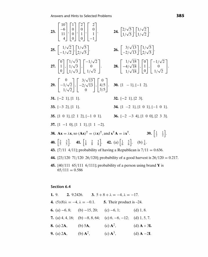
Answers and Hints to Selected Problems 385
23.
⎡⎢⎢⎣
10−6114
⎤⎥⎥⎦,
⎡⎢⎢⎣
1000
⎤⎥⎥⎦,
⎡⎢⎢⎣
2010
⎤⎥⎥⎦,
⎡⎢⎢⎣
201
−1
⎤⎥⎥⎦. 24.
[2/
√5
1/√
5
],
[1/
√2
1/√
2
].
25.[
1/√
2−1/
√2
],
[1/
√5
2/√
5
]. 26.
[3/
√13
−2/√
13
],
[1/
√5
2/√
5
].
27.
⎡⎣0
10
⎤⎦,
⎡⎣1/
√3
1/√
31/
√3
⎤⎦,
⎡⎣−1/
√2
01/
√2
⎤⎦. 28.
⎡⎣ 1/
√18
−4/√
181/
√18
⎤⎦,
⎡⎣0
10
⎤⎦,
⎡⎣−1/
√2
01/
√2
⎤⎦.
29.
⎡⎣ 0
−1/√
21/
√2
⎤⎦,
⎡⎣ 3/
√13
−2/√
130
⎤⎦,
⎡⎣ 0
4/53/5
⎤⎦. 30. [1 − 1], [−1 2].
31. [−2 1], [1 1]. 32. [−2 1], [2 3].33. [−3 2], [1 1]. 34. [1 −2 1], [1 0 1], [−1 0 1].
35. [1 0 1], [2 1 2], [−1 0 1]. 36. [−2 −3 4], [1 0 0], [2 3 3].37. [1 −1 0], [1 1 1], [1 1 −2].38. Ax = λx, so (Ax)T = (λx)T, and xTA = λxT. 39.
[12
12
].
40.[
25
35
]. 41.
[18
28
58
]. 42. (a)
[16
56
]. (b) 1
6 .
43. [7/11 4/11]; probability of having a Republican is 7/11 = 0.636.
44. [23/120 71/120 26/120]; probability of a good harvest is 26/120 = 0.217.
45. [40/111 65/111 6/111]; probability of a person using brand Y is65/111 = 0.586
Section 6.4
1. 9. 2. 9.2426. 3. 5 + 8 + λ = −4, λ = −17.
4. (5)(8)λ = −4, λ = −0.1. 5. Their product is –24.
6. (a) −6, 8; (b) −15, 20; (c) −6, 1; (d) 1, 8.
7. (a) 4, 4, 16; (b) −8, 8, 64; (c) 6, −6, −12; (d) 1, 5, 7.
8. (a) 2A, (b) 5A, (c) A2, (d) A + 3I.
9. (a) 2A, (b) A2, (c) A3, (d) A −2I.

386 Answers and Hints to Selected Problems
Section 6.5
1.[
1−1
]. 2.
[10
]. 3.
[10
],
[01
]. 4.
⎡⎣ 1
0−1
⎤⎦,
⎡⎣ 1
−10
⎤⎦,
⎡⎣1
01
⎤⎦.
5.
⎡⎣ 1
0−1
⎤⎦ ,
⎡⎣1
01
⎤⎦. 6.
⎡⎣0
10
⎤⎦,
⎡⎣1
01
⎤⎦,
⎡⎣ 1
2−1
⎤⎦. 7.
⎡⎣ 5
−41
⎤⎦,
⎡⎣−1
01
⎤⎦.
8.
⎡⎣ 3
0−1
⎤⎦,
⎡⎣−1
5−3
⎤⎦,
⎡⎣1
23
⎤⎦. 9.
⎡⎣ 1
0−1
⎤⎦,
⎡⎣1
21
⎤⎦,
⎡⎣ 1
−11
⎤⎦. 10.
⎡⎣1
39
⎤⎦.
11.
⎡⎣1
11
⎤⎦. 12.
⎡⎣ 1
0−1
⎤⎦,
⎡⎣1
21
⎤⎦,
⎡⎣ 1
−11
⎤⎦. 13.
⎡⎢⎢⎣
1111
⎤⎥⎥⎦.
14.
⎡⎢⎢⎣
1000
⎤⎥⎥⎦,
⎡⎢⎢⎣
0111
⎤⎥⎥⎦. 15.
⎡⎢⎢⎣
−1001
⎤⎥⎥⎦,
⎡⎢⎢⎣
−1010
⎤⎥⎥⎦,
⎡⎢⎢⎣
−1001
⎤⎥⎥⎦,
⎡⎢⎢⎣
0111
⎤⎥⎥⎦.
16.
⎡⎢⎢⎣
1000
⎤⎥⎥⎦,
⎡⎢⎢⎣
0−1
10
⎤⎥⎥⎦,
⎡⎢⎢⎣
−1−1
01
⎤⎥⎥⎦.
Section 6.6
1. Iteration Eigenvector components Eigenvalue0 1.0000 1.00001 0.6000 1.0000 5.00002 0.5238 1.0000 4.20003 0.5059 1.0000 4.04764 0.5015 1.0000 4.01185 0.5004 1.0000 4.0029
2. Iteration Eigenvector components Eigenvalue0 1.0000 1.00001 0.5000 1.0000 10.00002 0.5000 1.0000 8.00003 0.5000 1.0000 8.0000

Answers and Hints to Selected Problems 387
3. Iteration Eigenvector components Eigenvalue0 1.0000 1.00001 0.6000 1.0000 15.00002 0.6842 1.0000 11.40003 0.6623 1.0000 12.15794 0.6678 1.0000 11.96105 0.6664 1.0000 12.0098
4. Iteration Eigenvector components Eigenvalue0 1.0000 1.00001 0.5000 1.0000 2.00002 0.2500 1.0000 4.00003 0.2000 1.0000 5.00004 0.1923 1.0000 5.20005 0.1912 1.0000 5.2308
5. Iteration Eigenvector components Eigenvalue0 1.0000 1.00001 1.0000 0.6000 10.00002 1.0000 0.5217 9.20003 1.0000 0.5048 9.04354 1.0000 0.5011 9.00965 1.0000 0.5002 9.0021
6. Iteration Eigenvector components Eigenvalue0 1.0000 1.00001 1.0000 0.4545 11.00002 1.0000 0.4175 9.36363 1.0000 0.4145 9.25244 1.0000 0.4142 9.24345 1.0000 0.4142 9.2427
7. Iteration Eigenvector components Eigenvalue0 1.0000 1.0000 1.00001 0.2500 1.0000 0.8333 12.00002 0.0763 1.0000 0.7797 9.83333 0.0247 1.0000 0.7605 9.27124 0.0081 1.0000 0.7537 9.09145 0.0027 1.0000 0.7513 9.0310

388 Answers and Hints to Selected Problems
8. Iteration Eigenvector components Eigenvalue0 1.0000 1.0000 1.00001 0.6923 0.6923 1.0000 13.00002 0.5586 0.7241 1.0000 11.15383 0.4723 0.6912 1.0000 11.34484 0.4206 0.6850 1.0000 11.14715 0.3883 0.6774 1.0000 11.1101
9. Iteration Eigenvector components Eigenvalue0 1.0000 1.0000 1.00001 0.4000 0.7000 1.0000 20.00002 0.3415 0.6707 1.0000 16.40003 0.3343 0.6672 1.0000 16.04884 0.3335 0.6667 1.0000 16.00615 0.3333 0.6667 1.0000 16.0008
10. Iteration Eigenvector components Eigenvalue0 1.0000 1.0000 1.00001 0.4000 1.0000 0.3000 −20.00002 1.0000 0.7447 0.0284 −14.10003 0.5244 1.0000 −0.3683 −19.95044 1.0000 0.7168 −0.5303 −18.52935 0.6814 1.0000 −0.7423 −20.3976
11.
⎡⎣1
11
⎤⎦ is a linear combination of
⎡⎣ 1
−41
⎤⎦ and
⎡⎣0
10
⎤⎦, which are eigenvectors
corresponding to λ = 1 and λ = 2, not λ = 3. Thus, the power method con-verges to λ = 2.
12. There is no single dominant eigenvalue. Here, |λ1| = |λ2| = √34.
13. Shift by λ = 4. Power method on A =[−2 1
2 −1
]converges after three
iterations to μ = −3. λ + μ = 1.
14. Shift by λ = 16. Power method on A =⎡⎣−13 2 3
2 −10 63 6 −5
⎤⎦ converges after
three iterations to μ = −14. λ + μ = 2.

Answers and Hints to Selected Problems 389
15. Iteration Eigenvector components Eigenvalue0 1.0000 1.00001 −0.3333 1.0000 0.60002 1.0000 −0.7778 0.60003 −0.9535 1.0000 0.95564 1.0000 0.9904 0.97215 −0.9981 1.0000 0.9981
16. Iteration Eigenvector components Eigenvalue0 1.0000 −0.50001 −0.8571 1.0000 0.29172 1.0000 −0.9615 0.30953 −0.9903 1.0000 0.33014 1.0000 0.9976 0.33175 −0.9994 1.0000 0.3331
17. Iteration Eigenvector components Eigenvalue0 1.0000 1.00001 0.2000 1.0000 0.27782 −0.1892 1.0000 0.41113 −0.2997 1.0000 0.47604 −0.3258 1.0000 0.49445 −0.3316 1.0000 0.4987
18. Iteration Eigenvector components Eigenvalue0 1.0000 1.00001 −0.2000 1.0000 0.71432 −0.3953 1.0000 1.22863 −0.4127 1.0000 1.31234 −0.4141 1.0000 1.31975 −0.4142 1.0000 1.3203
19. Iteration Eigenvector components Eigenvalue0 1.0000 1.0000 1.00001 1.0000 0.4000 −0.2000 0.31252 1.0000 0.2703 −0.4595 0.46253 1.0000 0.2526 −0.4949 0.49494 1.0000 0.2503 −0.4994 0.49945 1.0000 0.2500 −0.4999 0.4999

390 Answers and Hints to Selected Problems
20. Iteration Eigenvector components Eigenvalue0 1.0000 1.0000 1.00001 0.3846 1.0000 0.9487 −0.10432 0.5004 0.7042 1.0000 −0.09693 0.3296 0.7720 1.0000 −0.09164 0.3857 0.6633 1.0000 −0.09405 0.3244 0.7002 1.0000 −0.0907
21. Iteration Eigenvector components Eigenvalue0 1.0000 1.0000 1.00001 −0.6667 1.0000 −0.6667 −1.50002 −0.3636 1.0000 −0.3636 1.83333 −0.2963 1.0000 −0.2963 1.22734 −0.2712 1.0000 −0.2712 1.09265 −0.2602 1.0000 −0.2602 1.0424
22. Cannot construct an LU decomposition. Shift as explained in Problem 13.
23. Cannot solve Lx1 = y uniquely for x1 because one eigenvalue is zero. Shift asexplained in Problem 13.
24. Yes, on occasion.
25. Inverse power method applied to A =⎡⎣−7 2 3
2 −4 63 6 1
⎤⎦ converges to μ = 1/6.
λ + 1/μ = 10 + 6 = 16.
26. Inverse power method applied to A =⎡⎣ 27 −17 7
−17 21 17 1 11
⎤⎦ converges to
μ = 1/3. λ + 1/μ = −25 + 3 = −22.
CHAPTER 7
Section 7.1
1. (a)
⎡⎣0 −4 8
0 4 −80 0 0
⎤⎦,
⎡⎣0 8 −16
0 −8 160 0 0
⎤⎦; (b)
[57 78
117 174
],[
234 348522 756
].
2. pk(A) =⎡⎣pk(λ1) 0 0
0 pk(λ2) 00 0 pk(λ3)
⎤⎦. 4. In general, AB �= BA.

Answers and Hints to Selected Problems 391
5. Yes. 6.[
0 23 0
]. 7.
⎡⎣ 2
03/2
⎤⎦.
8. 2−2 element tends to ∞, so limit diverges. 9. a, b, d, and f .
10. f . 11. All except c. 13.[e 00 e2
]. 14.
[e−1 0
0 e28
].
15.
⎡⎣e2 0 0
0 e−2 00 0 1
⎤⎦. 16. sin(A) =
⎡⎢⎢⎢⎣
sin(λ1) 0 · · · 00 sin(λ2) · · · 0...
... . . ....
0 0 · · · sin(λn)
⎤⎥⎥⎥⎦.
17.[
sin(1) 00 sin(2)
]. 18.
[sin(−1) 0
0 sin(28)
].
19. cos A =∞∑
k=0
(−1)kA2k
(2k)! , cos[
1 00 2
]=[
cos(1) 00 cos(2)
].
20.
⎡⎣cos(2) 0 0
0 cos(−2) 00 0 1
⎤⎦.
Section 7.2
1. A−1 =[−2 1
3/2 −1/2
]. 2. Since α0 = 0, the inverse does not exist.
3. Since α0 = 0, the inverse does not exist.
4. A−1
⎡⎣−1/3 −1/3 2/3
−1/3 1/6 1/61/2 1/4 −1/4
⎤⎦. 5. A−1 =
⎡⎢⎢⎣
1 0 0 00 −1 0 00 0 −1 00 0 0 1
⎤⎥⎥⎦.
Section 7.3
1.1 = α1 + α0,
−1 = −α1 + α0;[−2 3−1 2
]. 2.
[1 00 1
].
3.0 = α0,
−1 = −α1 + α0;[
0 10 −1
].
4.0 = α01 = −α1 + α0;
[3 −61 −2
]. 5.
[−3 6−1 2
]. 6.
[0 −10 1
].

392 Answers and Hints to Selected Problems
7.378 = 3α1 + α0,
478 = 478 = 4α1 + α0;
[−478 + 2
(378) −478 + 378
2(478)− 2
(378) 2
(478)− 378
].
8.
[−441 + 2
(341) −441 + 341
2(441)− 2
(341) 2
(441)− 341
].
9. 1 = α2 + α1 + α0,
1 = α2 − α1 + α0,
2222 = 4α2 + 2α1 + α0;
⎡⎢⎣
1 0(−4 + 4
(2222))/3
0 1(−2 + 2
(2222))/3
0 0 2222
⎤⎥⎦.
10. 317 = 9α2 + 3α1 + α0,
517 = 25α2 + 5α1 + α0,
1017 = 100α2 + 10α1 + α0.
11. 225 = 8α3 + 4α2 + 2α1 + α0,
(−2)25 = −8α3 + 4α2 − 2α1 + α0,
325 = 27α3 + 9α2 + 3α1 + α0,
425 = 64α3 + 16α2 + 4α1 + α0.
12. 1 = α3 + α2 + α1 + α0,
(−2)25 = −8α3 + 4α2 − 2α1 + α0,
325 = 27α3 + 9α2 + 3α1 + α0,(−425) = −64α3 + 16α2 − 4α1 + α0.
13. 1 = α4 + α3 + α2 + α1 + α0,
1 = α4 − α3 + α2 − α1 + α0,
256 = 16α4 + 8α3 + 4α2 + 2α1 + α0,
256 = 16α4 − 8α3 + 4α2 − 2α1 + α0,
6,561 = 81α4 + 27α3 + 9α2 + 3α1 + α0.
14. 5,837 = 9α2 + 3α1 + α0,
381,255 = 25α2 + 5α1 + α0,
108 − 3 (10)5 + 5 = 100α2 + 10α1 + α0.
15. 165 = 8α3 + 4α2 + 2α1 + α0,
357 = −8α3 + 4α2 − 2α1 + α0,
5,837 = 27α3 + 9α2 + 3α1 + α0,
62,469 = 64α3 + 16α2 + 4α1 + α0.
16. 3 = α3 + α2 + α1 + α0,
357 = −8α3 + 4α2 − 2α1 + α0,
5,837 = 27α3 + 9α2 + 3α1 + α0,
68,613 = −64α3 + 16α2 − 4α1 + α0.
17. 15 = α3 + α2 + α1 + α0,
960 = −8α3 + 4α2 − 2α1 + α0,
59,235 = 27α3 + 9α2 + 3α1 + α0,
1,048,160 = −64α3 + 16α2 − 4α1 + α0.

Answers and Hints to Selected Problems 393
18. 15 = α4 + α3 + α2 + α1 + α0,
−13 = α4 − α3 + α2 − α1 + α0,
1,088 = 16α4 + 8α3 + 4α2 + 2α1 + α0,
960 = 16α4 − 8α3 + 4α2 − 2α1 + α0,
59,235 = 81α4 + 27α3 + 9α2 + 3α1 + α0.
19.[
9 −93 −3
]. 20.
[6 −93 −6
]. 21.
[−50,801 −56,632113,264 119,095
].
22.[
3,007 −5,1201,024 −3,067
]. 23.
[938 160−32 1130
]. 24.
⎡⎣2 −4 −3
0 0 01 −5 −2
⎤⎦.
25. 2, 569 = 4α2 + 2α1 + α0,
5, 633 = 4α2 − 2α1 + α0,
5 = α2 + α1 + α0.
⎡⎣ −339 −766 1110
−4440 4101 344−1376 −3064 4445
⎤⎦.
26. 0.814453 = 0.25α2 + 0.5α1 + α0,
0.810547 = 0.25α2 − 0.5α1 + α0,
0.988285 = 0.0625α2 + 0.25α1 + α0.
⎡⎣1.045578 0.003906 −0.932312
0.058270 0.812500 −0.2291720.014323 0.000977 0.755207
⎤⎦.
Section 7.4
1. 128 = 2α1 + α0,
448 = α1.
2. 128 = 4α2 + 2α1 + α0,
448 = 4α2 + α1,
1,344 = 2α2.
3. 128 = 4α2 + 2α1 + α0,
448 = 4α2 + α1,
1 = α2 + α1 + α0.
4. 59,049 = 3α1 + α0,
196,830 = α1.
5. 59,049 = 9α2 + 3α1 + α0,
196,830 = 6α2 + α1,
590,490 = 2α2.
6. 59,049 = 27α3 + 9α2 + 3α1 + α0,
196,830 = 27α3 + 6α2 + α1,
590,490 = 18α3 + 2α2,
1,574,640 = 6α3.
7. 512 = 8α3 + 4α2 + 2α1 + α0,
2,304 = 12α3 + 4α2 + α1,
9,216 = 12α3 + 2α2,
32,256 = 6α3.
8. 512 = 8α3 + 4α2 + 2α1 + α0,
2,304 = 12α3 + 4α2 + α1,
9,216 = 12α3 + 2α2,
1 = α3 + α2 + α1 + α0.
9. 512 = 8α3 + 4α2 + 2α1 + α0,
2,304 = 12α3 + 4α2 + α1,
1 = α3 + α2 + α1 + α0.
9 = 3α3 + 2α2 + α1.
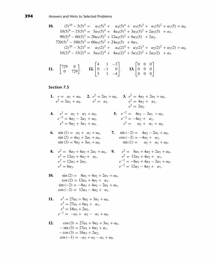
394 Answers and Hints to Selected Problems
10. (5)10 − 3(5)5 = α5(5)5 + α4(5)4 + α3(5)3 + α2(5)2 + α1(5) + α0,
10(5)9 − 15(5)4 = 5α5(5)4 + 4α4(5)3 + 3α3(5)2 + 2α2(5) + α1,
90(5)8 − 60(5)3 = 20α5(5)3 + 12α4(5)2 + 6α3(5) + 2α2,
720(5)7 − 180(5)2 = 60α5(5)2 + 24α4(5) + 6α3,
(2)10 − 3(2)5 = α5(2)5 + α4(2)4 + α3(2)3 + α2(2)2 + α1(2) + α0,
10(2)9 − 15(2)4 = 5α5(2)4 + 4α4(2)3 + 3α3(2)2 + 2α2(2) + α1.
11.[
729 00 729
]. 12.
⎡⎣4 1 −3
0 −1 05 1 −4
⎤⎦. 13.
⎡⎣0 0 0
0 0 00 0 0
⎤⎦.
Section 7.5
1. e = α1 + α0,
e2 = 2α1 + α0.
2. e2 = 2α1 + α0,
e2 = α1.
3. e2 = 4α2 + 2α1 + α0,
e2 = 4α2 + α1,
e2 = 2α2.
4. e1 = α2 + α1 + α0, 5. e−2 = 4α2 − 2α1 + α0,
e−2 = 4α2 − 2α1 + α0, e−2 = −4α2 + α1,
e3 = 9α2 + 3α1 + α0. e1 = α2 + α1 + α0.
6. sin (1) = α2 + α1 + α0, 7. sin (−2) = 4α2 − 2α1 + α0,
sin (2) = 4α2 + 2α1 + α0, cos (−2) = −4α2 + α1,
sin (3) = 9α2 + 3α1 + α0. sin (1) = α2 + α1 + α0.
8. e2 = 8α3 + 4α2 + 2α1 + α0, 9. e2 = 8α3 + 4α2 + 2α1 + α0,
e2 = 12α3 + 4α2 + α1, e2 = 12α3 + 4α2 + α1,
e2 = 12α3 + 2α2, e−2 = −8α3 + 4α2 − 2α1 + α0,
e2 = 6α3. e−2 = 12α3 − 4α2 + α1.
10. sin (2) = 8α3 + 4α2 + 2α1 + α0,
cos (2) = 12α3 + 4α2 + α1,
sin (−2) = −8α3 + 4α2 − 2α1 + α0,
cos (−2) = 12α3 − 4α2 + α1.
11. e3 = 27α3 + 9α2 + 3α1 + α0,
e3 = 27α3 + 6α2 + α1,
e3 = 18α3 + 2α2,
e−1 = −α3 + α2 − α1 + α0.
12. cos (3) = 27α3 + 9α2 + 3α1 + α0,
− sin (3) = 27α3 + 6α2 + α1,
− cos (3) = 18α3 + 2α2,
cos (−1) = −α3 + α2 − α1 + α0.

Answers and Hints to Selected Problems 395
13. 17
[3e5 + 4e−2 3e5 − 3e−2
4e5 − 4e−2 4e5 + 3e−2
]. 14. e3
[2 −11 0
].
15. e2
⎡⎣ 0 1 3
−1 2 50 0 1
⎤⎦. 16.
116
⎡⎣12e2 + 4e−2 4e2 − 4e−2 38e2 + 2e−2
12e2 − 12e−2 4e2 + 12e−2 46e2 − 6e−2
0 0 16e2
⎤⎦.
17. 15
[−1 64 1
].
18. (a)[
log(3/2) log(3/2) − log(1/2)
0 log(1/2)
].
(b) and (c) are not defined since they possess eigenvalues having absolutevalue greater than 1.
(d)[
0 00 0
].
Section 7.6
1. 1/7[
3e8t + 4et 4e8t − 4et
3e8t − 3et 4e8t + 3et
].
2.
[(2/
√3) sinh
√3t + cosh
√3t (1/
√3) sinh
√3t
(−1/√
3) sinh√
3t (−2/√
3) sinh√
3t + cosh√
3t
].
Note:
sinh√
3t = e√
3t − e−√3t
2and cosh
√3t = e
√3t + e−√
3t
2.
3. e3t
[1 + t t
−t 1 − t
]. 4.
[1.4e−2t − 0.4e−7t 0.2e−2t − 0.2e−7t
−2.8e−2t + 2.8e−7t −0.4e−2t + 1.4e−7t
].
5.[
0.8e−2t + 0.2e−7t 0.4e−2t − 0.4e−7t
0.4e−2t − 0.4e−7t 0.2e−2t + 0.8e−7t
].
6.[
0.5e−4t + 0.5e−16t 0.5e−4t − 0.5e−16t
0.5e−4t − 0.5e−16t 0.5e−4t + 0.5e−16t
].
7.
⎡⎣1 t t2/2
0 1 t
0 0 1
⎤⎦.

396 Answers and Hints to Selected Problems
8.1
12
⎡⎣ 12et 0 0
−9et + 14e3t − 5e−3t 8e3t + 4e−3t 4e3t − 4e−3t
−24et + 14e3t + 10e−3t 8e3t − 8e−3t 4e3t + 8e−3t
⎤⎦.
Section 7.7
1.
[(1/2) sin 2t + cos 2t (−1/2) sin 2t
(5/2) sin 2t (−1/2) sin 2t + cos 2t
].
2.
[√2 sin
√2t + cos
√2t −√
2 sin√
2t
(3/√
2) sin√
2t −√2 sin
√2t + cos
√2t
].
3.
[cos(8t) 1
8 sin(8t)
−8 sin(8t) cos(8t)
].
4.14
[2 sin(8t) + 4 cos(8t) −4 sin(8t)
5 sin(8t) −2 sin(8t) + 4 cos(8t)
].
5.[
2 sin(t) + cos(t) 5 sin(t)
− sin(t) −2 sin(t) + cos(t)
].
6.13e−4t
[4 sin(3t) + 3 cos(3t) sin(3t)
−25 sin(3t) −4 sin(3t) + 3 cos(3t)
].
7. e4t
[− sin t + cos t sin t
−2 sin t sin t + cos t
].
8.
⎡⎣1 −2 + 2 cos(t) + sin(t) −5 + 5 cos(t)
0 cos(t) − 2 sin(t) −5 sin(t)
0 sin(t) cos(t) + 2 sin(t)
⎤⎦.
Section 7.8
3. A does not have an inverse.
8. eA =[e e − 10 1
], eB =
[1 e − 10 1
], eAeB =
[e 2e2 − 2e
0 e
],
eBeA =[e 2e − 20 e
], eA+B =
[e 2e
0 e
].
9. A =[
1 00 2
], B =
[3 00 4
]. Also see Problem 10.
11. First show that for any integer n, (P−1BP)n = P−1BnP, and then use Eq. (6)directly.

Answers and Hints to Selected Problems 397
Section 7.9
1. (a)[− sin t 2t
2 e(t−1)
]. (b)
⎡⎢⎣ 6t2et3 2t − 1 0
2t + 3 2 cos 2t 1
−18t cos2(3t2) sin(3t2) 0 1/t
⎤⎥⎦.
4.
[sin t + c1
13 t3 − t + c2
t2 + c3 e(t−1) + c4
].
CHAPTER 8
Section 8.1
1. x(t) =[x(t)
y(t)
], A(t) =
[2 34 5
], f(t) =
[00
], c =
[67
], t0 = 0.
2. x(t) =[y(t)
z(t)
], A(t) =
[3 24 1
], f(t) =
[00
], c =
[11
], t0 = 0.
3. x(t) =[x(t)
y(t)
], A(t) =
[−3 34 −4
], f(t) =
[1
−1
], c =
[00
], t0 = 0.
4. x(t) =[x(t)
y(t)
], A(t) =
[3 02 0
], f(t) =
[t
t + 1
], c =
[1
−1
], t0 = 0.
5. x(t) =[x(t)
y(t)
], A(t) =
[3t2 71 t
], f(t) =
[22t
], c =
[2
−3
], t0 = 1.
6. x(t) =⎡⎣u(t)
v(t)
w(t)
⎤⎦, A(t) =
⎡⎣et t 1
t2 −3 t + 10 1 et2
⎤⎦, f(t) =
⎡⎣0
00
⎤⎦, c =
⎡⎣ 0
1−1
⎤⎦, t0 = 4.
7. x(t) =⎡⎣x(t)
y(t)
z(t)
⎤⎦, A(t) =
⎡⎣0 6 1
1 0 −30 −2 0
⎤⎦, f(t) =
⎡⎣0
00
⎤⎦, c =
⎡⎣10
1020
⎤⎦, t0 = 0.
8. x(t) =⎡⎣r(t)
s(t)
u(t)
⎤⎦, A(t) =
⎡⎣t2 −3 − sin t
1 −1 02 et t2 − 1
⎤⎦, f(t) =
⎡⎣ sin t
t2 − 1cos t
⎤⎦,
c =⎡⎣ 4
−25
⎤⎦, t0 = 1.
9. Only (c). 10. Only (c). 11. Only (b).

398 Answers and Hints to Selected Problems
Section 8.2
1. x(t) =[x1(t)
x2(t)
], A(t) =
[0 13 2
], f(t) =
[00
], c =
[45
], t0 = 0.
2. x(t) =[x1(t)
x2(t)
], A(t) =
[0 1t −et
], f(t) =
[00
], c =
[20
], t0 = 1.
3. x(t) =[x1(t)
x2(t)
], A(t) =
[0 11 0
], f(t) =
[0t2
], c =
[−33
], t0 = 0.
4. x(t) =[x1(t)
x2(t)
], A(t) =
[0 13 2et
], f(t) =
[0
2e−t
], c =
[00
], t0 = 0.
5. x(t) =[x1(t)
x2(t)
], A(t) =
[0 1
−2 3
], f(t) =
[0
e−t
], c =
[22
], t0 = 1.
6. x(t) =⎡⎣x1(t)
x2(t)
x3(t)
⎤⎦, A(t) =
⎡⎣ 0 1 0
0 0 11/4 0 −t/4
⎤⎦, f(t) =
⎡⎣0
00
⎤⎦, c =
⎡⎣ 2
1−205
⎤⎦,
t0 = −1.
7. x(t) =
⎡⎢⎢⎣
x1(t)
x2(t)
x3(t)
x4(t)
⎤⎥⎥⎦, A(t) =
⎡⎢⎢⎢⎣
0 1 0 00 0 1 00 0 0 10 e−t −te−t 0
⎤⎥⎥⎥⎦, f(t) =
⎡⎢⎢⎣
000
e−t
⎤⎥⎥⎦, c =
⎡⎢⎢⎣
12π
e3
⎤⎥⎥⎦,
t0 = 0.
8. x(t) =
⎡⎢⎢⎢⎢⎢⎢⎣
x1(t)
x2(t)
x3(t)
x4(t)
x5(t)
x6(t)
⎤⎥⎥⎥⎥⎥⎥⎦, A(t) =
⎡⎢⎢⎢⎢⎢⎢⎣
0 1 0 0 0 00 0 1 0 0 00 0 0 1 0 00 0 0 0 1 00 0 0 0 0 10 0 0 0 −4 0
⎤⎥⎥⎥⎥⎥⎥⎦, f(t) =
⎡⎢⎢⎢⎢⎢⎢⎣
00000
t2 − t
⎤⎥⎥⎥⎥⎥⎥⎦,
c =
⎡⎢⎢⎢⎢⎢⎢⎣
210210
⎤⎥⎥⎥⎥⎥⎥⎦, t0 = π.

Answers and Hints to Selected Problems 399
Section 8.3
1. x(t) =⎡⎣x1(t)
x2(t)
y1(t)
⎤⎦, A(t) =
⎡⎣0 1 0
3 2 45 0 −6
⎤⎦, f(t) =
⎡⎣0
00
⎤⎦, c =
⎡⎣7
89
⎤⎦, t0 = 0.
2. x(t) =
⎡⎢⎢⎣
x1(t)
x2(t)
y1(t)
y2(t)
⎤⎥⎥⎦, A(t) =
⎡⎢⎢⎣
0 1 0 00 1 0 10 0 0 10 −1 0 1
⎤⎥⎥⎦, f(t) =
⎡⎢⎢⎣
0000
⎤⎥⎥⎦, c =
⎡⎢⎢⎣
2344
⎤⎥⎥⎦, t0 = 0.
3. x(t) =⎡⎣x1(t)
y1(t)
y2(t)
⎤⎦, A(t) =
⎡⎣−4 0 t2
0 0 1t2 t 0
⎤⎦, f(t) =
⎡⎣0
00
⎤⎦, c =
⎡⎣−1
00
⎤⎦, t0 = 2.
4. x(t) =⎡⎣x1(t)
y1(t)
y2(t)
⎤⎦, A(t) =
⎡⎣−4 0 2
0 0 13 t 0
⎤⎦, f(t) =
⎡⎣ t
0−1
⎤⎦, c =
⎡⎣0
00
⎤⎦, t0 = 3.
5. x(t) =
⎡⎢⎢⎢⎢⎢⎢⎣
x1(t)
x2(t)
y1(t)
y2(t)
y3(t)
y4(t)
⎤⎥⎥⎥⎥⎥⎥⎦, A(t) =
⎡⎢⎢⎢⎢⎢⎢⎣
0 1 0 0 0 00 2 0 0 0 10 0 0 1 0 00 0 0 0 1 00 0 0 0 0 1t 0 −t 0 1 0
⎤⎥⎥⎥⎥⎥⎥⎦, f(t) =
⎡⎢⎢⎢⎢⎢⎢⎣
0−t
000
−et
⎤⎥⎥⎥⎥⎥⎥⎦,
c =
⎡⎢⎢⎢⎢⎢⎢⎣
200394
⎤⎥⎥⎥⎥⎥⎥⎦, t0 = −1.
6. x(t) =
⎡⎢⎢⎢⎢⎣
x1(t)
x2(t)
x3(t)
y1(t)
y2(t)
⎤⎥⎥⎥⎥⎦, A(t) =
⎡⎢⎢⎢⎢⎣
0 1 0 0 00 0 1 0 01 0 0 −1 10 0 0 0 1
−1 0 1 0 2
⎤⎥⎥⎥⎥⎦, f(t) =
⎡⎢⎢⎢⎢⎣
00000
⎤⎥⎥⎥⎥⎦,
c =
⎡⎢⎢⎢⎢⎣
214
−557
⎤⎥⎥⎥⎥⎦, t0 = 0.

400 Answers and Hints to Selected Problems
7. x(t) =
⎡⎢⎢⎣
x1(t)
y1(t)
y2(t)
z1(t)
⎤⎥⎥⎦, A(t) =
⎡⎢⎢⎣
0 1 0 00 0 1 00 0 0 11 1 0 0
⎤⎥⎥⎦, f(t) =
⎡⎢⎢⎣
−20
−20
⎤⎥⎥⎦, c =
⎡⎢⎢⎣
12
170
⎤⎥⎥⎦, t0 = π.
8. x(t) =
⎡⎢⎢⎢⎢⎢⎢⎣
x1(t)
x2(t)
y1(t)
y2(t)
z1(t)
z2(t)
⎤⎥⎥⎥⎥⎥⎥⎦, A(t) =
⎡⎢⎢⎢⎢⎢⎢⎣
0 1 0 0 0 00 0 1 0 1 00 0 0 1 0 01 0 1 0 0 00 0 0 0 0 11 0 0 0 −1 0
⎤⎥⎥⎥⎥⎥⎥⎦, f(t) =
⎡⎢⎢⎢⎢⎢⎢⎣
020
−101
⎤⎥⎥⎥⎥⎥⎥⎦,
c =
⎡⎢⎢⎢⎢⎢⎢⎣
4−4
5−5
9−9
⎤⎥⎥⎥⎥⎥⎥⎦, t0 = 20.
Section 8.4
3. (a) e−3t
⎡⎣1 −t t2/2
0 1 −t
0 0 1
⎤⎦, (b) e3(t−2)
⎡⎣1 (t − 2) (t − 2)2/2
0 1 (t − 2)
0 0 1
⎤⎦,
(c) e3(t−s)
⎡⎣1 (t − 2) (t − s)2/2
0 1 (t − s)
0 0 1
⎤⎦,
(d) e−3(t−2)
⎡⎣1 −(t − 2) (t − 2)2/2
0 1 −(t − s)
0 0 1
⎤⎦.
5. (a)16
[2e−5t + 4et 2e−5t − 2et
4e−5t − 4et 4e−5t + 2et
], (b)
16
[2e−5s + 4es 2e−5s − 2es
4e−5s − 4es 4e−5s + 2es
],
(c)16
[2e5(t−3) + 4e−(t−3) 2e5(t−3) − 2e−(t−3)
4e5(t−3) − 4e−(t−3) 4e5(t−3) + 2e−(t−3)
].
6. (a)13
[sin 3t + 3 cos 3t −5 sin 3t
2 sin 3t − sin 3t + 3 cos 3t
],
(b)13
[sin 3s + 3 cos 3s −5 sin 3s
2 sin 3s − sin 3s + 3 cos 3s
],

Answers and Hints to Selected Problems 401
(c)13
[sin 3(t − s) + 3 cos 3(t − s) −5 sin 3(t − s)
2 sin 3(t − s) − sin 3(t − s) + 3 cos 3(t − s)t
].
7. x(t) = 5e(t−2) − 3e−(t−2), y(t) = 5e(t−2) − e−(t−2).
8. x(t) = 2e(t−1) − 1, y(t) = 2e(t−1) − 1.
9. x(t) = k3et + 3k4e
−t , y(t) = k3et + k4e
−t .
10. x(t) = k3et + 3k4e
−t − 1, y(t) = k3et + k4e
−t − 1.
11. x(t) = cos 2t − (1/6) sin 2t + (1/3) sin t.
12. x(t) = t4/24 + (5/4)t2 − (2/3)t + 3/8.
13. x(t) = (4/9) e2t + (5/9)e−1t − (1/3) te−1t
14. x(t) = −8 cos t − 6 sin t + 8 + 6t,
y(t) = 4 cos t − 2 sin t − 3.
Section 8.5
4. First show that
�T(t1, t0)
[∫ t1
t0
�(t1, s)�T(t1, s)ds
]−1
�(t1, t0)
=[�(t0, t1)
∫ t1
t0
�(t1, s)�′(t1, s)ds�T(t0, t1)
]−1
=[∫ t1
t0
�(t0, t1)�(t1, s)[�(t0, t1)�(t1, s)]Tds
]−1
.
CHAPTER 9
Section 9.1
1. (a) The English alphabet: a, b, c, . . . x, y, z. 26. 5/26.
(b) The 366 days designated by a 2008 Calendar, ranging from 1 Januarythrough 31 December. 366. 1/366.
(c) A list of all 43 United States Presidents. 43. 1/43.
(d) Same as (c). 43. 2/43 (Grover Cleveland was both the 22nd and 24th
President).
(e) Regular deck of 52 cards. 52. 1/52.
(f) Pinochle deck of 48 cards. 48. 2/48.
(g) See Figure 9.1 of Chapter 9. 36. 1/36.

402 Answers and Hints to Selected Problems
(h) Same as (g). (i) Same as (g). 5/36.
(j) Same as (g). 2/36. (k) Same as (g). 18/36.
(l) Same as (g). 7/36. (m) Same as (g). 5/36.
(n) Same as (g). 12/36. (o) Same as (n).
(p) Same as (g). 0.
2. The sample space would consist of all 216 possibilities, ranging from rolling a“3” to tossing an “18”.
3. 90. 4. 1950.
Section 9.2
1. (a) 8/52. (b) 16/52. (c) 28/52.
(d) 2/52. (e) 28/52. (f) 26/52.
(g) 39/52. (h) 48/52. (i) 36/52.
2. (a) 18/36. (b) 15/36. (c) 10/36.
(d) 30/36. (e) 26/36. (f) 1.
3. (a) 108/216. (b) 1/216. (c) 1/216.
(d) 3/216. (e) 3/216. (f) 0.
(g) 213/216. (h) 210/216. (i) 206/216.
4. 0.75. 5. 0.4.
6. P(A ∪ B ∪ C ∪ D) = P(A) + P(B) + P(C) + P(D) − P(A ∩ B) −P(A ∩ C) − P(A ∩ D) − P(B ∩ C) − P(B ∩ D) − P(C ∩ D) +P(A ∩ B ∩ C) + P(A ∩ B ∩ D) + P(A ∩ C ∩ D) +P(B ∩ C ∩ D) − P(A ∩ B ∩ C ∩ D).
Section 9.3
1. (a) 15. (b) 7. (c) 56. (d) 190.
(e) 190. (f) 1. (g) 1. (h) 100.
(i) 1000. (j) 1.
2. 2,042,975. 3. 5005.
4. (a) Approximately .372. (b) Approximately .104.
(c) Approximately .135. (d) Approximately .969.
(e) Approximately .767.

Answers and Hints to Selected Problems 403
5. (a)(
500123
)(.65)123 (.35)377.
(b)(
500485
)(.65)485 (.35)15.
(c)(
500497
)(.65)497 (.35)3 +
(500498
)(.65)498 (.35)2
+(
500499
) (.65)499 (
.35)1 +
(500500
) (.65)500 (
.35)0
.
(d) 1 −(
500498
) (.65)498 (
.35)2 −
(500499
) (.65)499 (
.35)1 −
(500500
) (.65)500 (
.35)0.
(e)(
500100
) (.65)100 (
.35)400 +
(500200
) (.65)200 (
.35)300 +
(500300
) (.65)300 (
.35)200
+(
500400
) (.65)400 (
.35)100 +
(500500
) (.65)500 (
.35)0
.
6. Approximately .267.
7. Approximately .267.
Section 9.4
1. (a) There is a negative element in the second row.
(b) The first row does not add to 1.
(c) The third row does not add to 1.
(d) It is not a square matrix.
2. (a) If it is sunny today, there is a probability of .5 that it will be sunny tomor-row and a .5 probability that it will rain tomorrow. If it rains today, there isa .7 probability that it will be sunny tomorrow and a .3 chance that it willrain tomorrow.
(b) If a parking meter works today, there is a probability of .95 that it willwork tomorrow with a .05 probability that it will not work tomorrow. If theparking meter is inoperative today, there is a probability of .02 that it willbe fixed tomorrow and a .98 probability that it will not be fixed tomorrow.
(c) Any scenario has a “50–50” chance at any stage.
(d) What is “good” stays “good”; what is “bad” stays “bad”.
(e) What is “good” today is “bad” tomorrow; what is “bad” today is “good”tomorrow.

404 Answers and Hints to Selected Problems
(f) See Example 2 in Section 9.4 and use Tinker, Evers, and Chance for Moe,Curly, and Larry and instead of visiting or staying home use “borrowing acar” or “not borrowing a car”.
3. Clearly if we raise either matrix to any power, we obtain the original matrix.
4. The even powers produce[
1 00 1
]and the odd powers give back the original
matrix. And situation repeats itself after an even number of time periods.
5. p(2)11 = 0.4, p
(2)21 = 0.15, p
(3)12 = 0.7, p
(3)22 = 0.825.
6. (a)[.7 .3.4 .6
](b) Approximately 0.5725.
(c) Approximately 0.5717.
CHAPTER 10
Section 10.1
1. 11, 5. 2. 8, 4. 3. −50, 74. 4. 63, 205.
5. 64, 68. 6. 6, 5. 7. 26, 24. 8. −30, 38.
9. 5/6, 7/18. 10. 5/√
6, 1. 11. 7/24, 1/3. 12. 0, 1400.
13. 2, 3. 14. 1, 1. 15. −19, 147. 16. −1/5, 1/5.
17. undefined, 6. 18.[
3/54/5
]. 19.
[4/
√41
−5/√
41
]. 20.
[7/
√58 3/
√58].
21.
⎡⎢⎣−4/
√34
3/√
34
−3/√
34
⎤⎥⎦. 22.
⎡⎣ 3/
√17
−2/√
17−2/
√17
⎤⎦. 23.
[2/
√21 4/
√21 1/
√21].
24.
⎡⎢⎢⎣
4/√
197−6/
√197
−9/√
1978/
√197
⎤⎥⎥⎦. 25.
[1/
√55 2/
√55 − 3
√55 4/
√55 − 5/
√55].
26[−3/
√259 8/
√259 11/
√259 − 4/
√259 7/
√259].
27. No vector x exists. 28. Yes, see Problem 12.
33. ‖x + y‖2 = 〈x + y, x + y〉 = 〈x, x〉 + 2〈x, y〉 + 〈y, y〉= ‖x‖2 + 2〈x, y〉 + ‖y‖2.
34. Show that ‖x − y‖2 = ‖x‖2 − 2〈x, y〉 + ‖y‖2, and then use Problem 33.
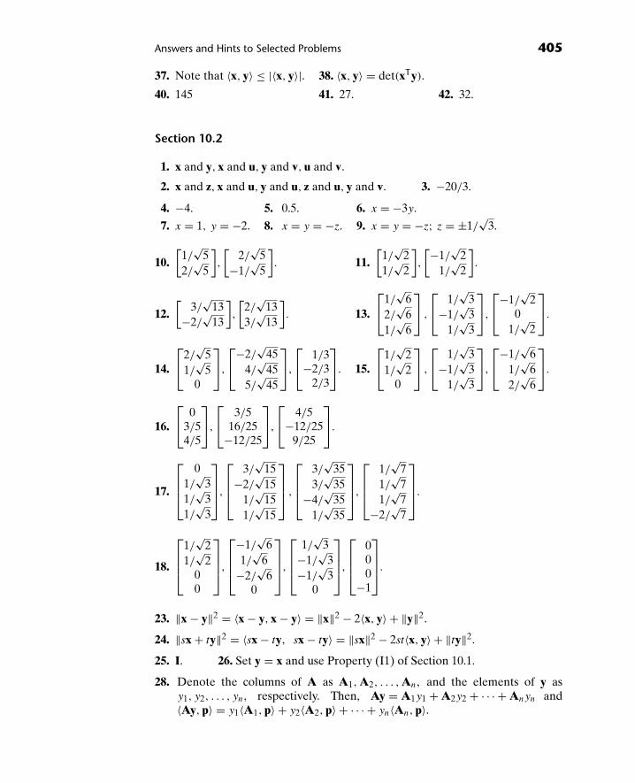
Answers and Hints to Selected Problems 405
37. Note that 〈x, y〉 ≤ |〈x, y〉|. 38. 〈x, y〉 = det(xTy).
40. 145 41. 27. 42. 32.
Section 10.2
1. x and y, x and u, y and v, u and v.
2. x and z, x and u, y and u, z and u, y and v. 3. −20/3.
4. −4. 5. 0.5. 6. x = −3y.
7. x = 1, y = −2. 8. x = y = −z. 9. x = y = −z; z = ±1/√
3.
10.[
1/√
52/
√5
],
[2/
√5
−1/√
5
]. 11.
[1/
√2
1/√
2
],
[−1/√
21/
√2
].
12.[
3/√
13−2/
√13
],
[2/
√13
3/√
13
]. 13.
⎡⎣1/
√6
2/√
61/
√6
⎤⎦ ,
⎡⎣ 1/
√3
−1/√
31/
√3
⎤⎦,
⎡⎣−1/
√2
01/
√2
⎤⎦.
14.
⎡⎣2/
√5
1/√
50
⎤⎦,
⎡⎣−2/
√45
4/√
455/
√45
⎤⎦,
⎡⎣ 1/3
−2/32/3
⎤⎦. 15.
⎡⎣1/
√2
1/√
20
⎤⎦ ,
⎡⎣ 1/
√3
−1/√
31/
√3
⎤⎦,
⎡⎣−1/
√6
1/√
62/
√6
⎤⎦.
16.
⎡⎣ 0
3/54/5
⎤⎦,
⎡⎣ 3/5
16/25−12/25
⎤⎦,
⎡⎣ 4/5
−12/259/25
⎤⎦.
17.
⎡⎢⎢⎣
01/
√3
1/√
31/
√3
⎤⎥⎥⎦,
⎡⎢⎢⎣
3/√
15−2/
√15
1/√
151/
√15
⎤⎥⎥⎦ ,
⎡⎢⎢⎣
3/√
353/
√35
−4/√
351/
√35
⎤⎥⎥⎦,
⎡⎢⎢⎣
1/√
71/
√7
1/√
7−2/
√7
⎤⎥⎥⎦.
18.
⎡⎢⎢⎣
1/√
21/
√2
00
⎤⎥⎥⎦,
⎡⎢⎢⎣
−1/√
61/
√6
−2/√
60
⎤⎥⎥⎦,
⎡⎢⎢⎣
1/√
3−1/
√3
−1/√
30
⎤⎥⎥⎦,
⎡⎢⎢⎣
000
−1
⎤⎥⎥⎦.
23. ‖x − y‖2 = 〈x − y, x − y〉 = ‖x‖2 − 2〈x, y〉 + ‖y‖2.
24. ‖sx + ty‖2 = 〈sx − ty, sx − ty〉 = ‖sx‖2 − 2st〈x, y〉 + ‖ty‖2.
25. I. 26. Set y = x and use Property (I1) of Section 10.1.
28. Denote the columns of A as A1, A2, . . . , An, and the elements of y asy1, y2, . . . , yn, respectively. Then, Ay = A1y1 + A2y2 + · · · + Anyn and〈Ay, p〉 = y1〈A1, p〉 + y2〈A2, p〉 + · · · + yn〈An, p〉.

406 Answers and Hints to Selected Problems
Section 10.3
1. (a) θ = 36.9◦, (b)[
1.60.8
], (c)
[−0.61.2
].
2. (a) θ = 14.0◦, (b)[
0.70591.1765
], (c)
[0.2941
−0.1765
].
3. (a) θ = 78.7◦, (b)[
0.50.5
], (c)
[2.5
−2.5
].
4. (a) θ = 90◦, (b)[
00
], (c)
[4
−1
].
5. (a) θ = 118.5◦, (b)[−0.7529−3.3882
], (c)
[−6.24711.3882
].
6. (a) θ = 50.8◦, (b)
⎡⎣1
01
⎤⎦, (c)
⎡⎣ 1
1−1
⎤⎦.
7. (a) θ = 19.5◦, (b)
⎡⎣8/9
8/94/9
⎤⎦, (c)
⎡⎣ 1/9
1/9−4/9
⎤⎦.
8. (a) θ = 17.7◦, (b)
⎡⎣1.2963
3.24073.2407
⎤⎦, (c)
⎡⎣−1.2963
−0.24070.7593
⎤⎦.
9. (a) θ = 48.2◦, (b)
⎡⎢⎢⎣
2/32/32/30
⎤⎥⎥⎦, (c)
⎡⎢⎢⎣
−2/31/31/31
⎤⎥⎥⎦.
10. (a) θ = 121.4◦, (b)
⎡⎢⎢⎣
−7/67/30
7/6
⎤⎥⎥⎦, (c)
⎡⎢⎢⎣
13/6−1/3
317/6
⎤⎥⎥⎦.
11.[
0.4472 0.89440.8944 −0.4472
] [2.2361 1.78890.0000 1.3416
].
12.[
0.7071 −0.70710.7071 0.7071
] [1.4142 5.65690.0000 1.4142
].
13.[
0.8321 0.5547−0.5547 0.8321
] [3.6056 0.83210.0000 4.1603
].

Answers and Hints to Selected Problems 407
14.
⎡⎣0.3333
0.66670.6667
0.80850.1617
−0.5659
⎤⎦[3.0000 2.6667
0.0000 1.3744
].
15.
⎡⎣0.3015
0.30150.9045
−0.2752−0.8808
0.3853
⎤⎦[3.3166 4.8242
0.0000 1.6514
].
16.
⎡⎢⎢⎣
0.7746−0.5164
0.2582−0.2582
0.40340.57140.47060.5378
⎤⎥⎥⎦[
3.8730 0.25820.0000 1.9833
].
17.
⎡⎣0.8944 −0.2981 0.3333
0.4472 0.5963 −0.66670.0000 0.7454 0.6667
⎤⎦⎡⎣2.2361 0.4472 1.7889
0.0000 1.3416 0.89440.0000 0.0000 2.0000
⎤⎦.
18.
⎡⎣0.7071 0.5774 −0.4082
0.7071 −0.5774 0.40820.0000 0.5774 0.8165
⎤⎦⎡⎣1.4142 1.4142 2.8284
0.0000 1.7321 0.57740.0000 0.0000 0.8165
⎤⎦.
19.
⎡⎣0.00 0.60 0.80
0.60 0.64 −0.480.80 −0.48 0.36
⎤⎦⎡⎣5 3 7
0 5 20 0 1
⎤⎦.
20.
⎡⎢⎢⎣
0.0000 0.7746 0.50710.5774 −0.5164 0.50710.5774 0.2582 −0.67610.5774 0.2582 0.1690
⎤⎥⎥⎦⎡⎣1.7321 1.1547 1.1547
0.0000 1.2910 0.51640.0000 0.0000 1.1832
⎤⎦.
21.
⎡⎢⎢⎣
0.7071 −0.4082 0.57740.7071 0.4082 −0.57740.0000 −0.8165 −0.57740.0000 0.0000 0.0000
⎤⎥⎥⎦⎡⎣1.4142 0.7071 0.7071
0.0000 1.2247 0.40820.0000 0.0000 1.1547
⎤⎦.
24. QR �= A.
Section 10.4
1. A1 = R0Q0 + 7I
=⎡⎣19.3132 −1.2945 0.0000
0.0000 7.0231 −0.99670.0000 0.0000 0.0811
⎤⎦⎡⎣−0.3624 0.0756 0.9289
0.0000 −0.9967 0.08110.9320 0.0294 0.3613
⎤⎦
+ 7
⎡⎣1 0 0
0 1 00 0 1
⎤⎦ =
⎡⎣ 0.0000 2.7499 17.8357
−0.9289 −0.0293 0.20950.0756 0.0024 7.0293
⎤⎦.

408 Answers and Hints to Selected Problems
2. A1 = R0Q0 − 14I
=⎡⎣24.3721 −17.8483 3.8979
0.0000 8.4522 −4.66500.0000 0.0000 3.6117
⎤⎦⎡⎣ 0.6565 −0.6250 0.4223
−0.6975 −0.2898 0.65530.2872 0.7248 0.6262
⎤⎦
−14
⎡⎣1 0 0
0 1 00 0 1
⎤⎦ =
⎡⎣ 15.5690 −7.2354 1.0373
−7.2354 −19.8307 2.61781.0373 2.6178 −11.7383
⎤⎦.
3. Shift by 4.
R0 =
⎡⎢⎢⎣
4.1231 −0.9701 0.0000 13.58200.0000 4.0073 −0.9982 −4.19820.0000 0.0000 4.0005 12.95090.0000 0.0000 0.0000 3.3435
⎤⎥⎥⎦,
Q0 =
⎡⎢⎢⎣
−0.9701 −0.2349 −0.0586 −0.01510.2425 −0.9395 −0.2344 −0.06050.0000 0.2495 −0.9376 −0.24210.0000 0.0000 0.2500 −0.9683
⎤⎥⎥⎦.
A1 = R0Q0 + 4I =
⎡⎢⎢⎣
−0.2353 −0.0570 3.3809 −13.15450.9719 −0.0138 −1.0529 4.06400.0000 0.9983 3.4864 −13.50810.0000 0.0000 0.8358 0.7626
⎤⎥⎥⎦.
4. 7.2077, −0.1039 ± 1.5769i. 5. −11, −22, 17. 6. 2, 3, 9.
7. Method fails. A0 − 7I does not have linearly independent columns, so no QR-decomposition is possible.
8. 2, 2, 16. 9. 1, 3, 3. 10. 2, 3 ± i. 11. 1, ± i.
12. ± i, 2 ± 3i. 13. 3.1265 ± 1.2638i, − 2.6265 ± 0.7590i.
14. 0.0102, 0.8431, 3.8581, 30.887.
Section 10.5
1. x = 2.225, y = 1.464. 2. x = 3.171, y = 2.286.
3. x = 9.879, y = 18.398. 4. x = −1.174, y = 8.105.
5. x = 1.512, y = 0.639, z = 0.945. 6. x = 7.845, y = 1.548, z = 5.190.
7. x = 81.003, y = 50.870, z = 38.801. 8. x = 2.818, y = −0.364, z = −1.364.
9. 2 and 4. 10. (b) y = 2.3x + 8.1, (c) 21.9.
11. (b) y = −2.6x + 54.4, (c) 31 in week 9, 28 in week 10.

Answers and Hints to Selected Problems 409
12. (b) y = 0.27x + 10.24, (c) 12.4.
13. m =N
N∑i=1
xiyi −N∑
i=1xi
N∑i=1
yi
NN∑
i=1x2i −
(N∑
i=1xi
)2 , c =
N∑i=1
yi
N∑i=1
x2i −
N∑i=1
xi
N∑i=1
xiyi
NN∑
i=1x2i −
(N∑
i=1xi
) .
If N∑N
i=1 x2i is near
(∑Ni=1 xi
)2, then the denominator is near zero.
14.∑N
i=1 x′i = 0, so the denominator for m and c as suggested in Problem 13 is
simply N∑N
i=1(x′i
)2.
15. y = 2.3x′ + 15. 16. y = −2.6x′ + 42.9.
17. (a) y = −0.198x′ + 21.18, (b) Year 2000 is coded as x′ = 30; y (30) = 15.2.
23. E =⎡⎣ 0.841
0.210−2.312
⎤⎦. 24. E =
⎡⎢⎢⎣
0.1600.069
−0.042−0.173
⎤⎥⎥⎦.

This page intentionally left blank

Index
AAdjacency matrices, 27–28, 42fAdjugates, 167–168Algorithms, 135
Gram-Schmidt, revised, 331–337QR, 339–344
Augmented matrix, 55–56
BBernoulli, Jakob, 305Bernoulli trials, 305–310
binomial distribution and, 305independent events and, 305multiplication rule for, 305
Binomial distribution, 305Normal Approximation to
Binomial Distribution, 314Block diagonals, 31Bounded regions. See Finite regions;
Regions
CCalculations, for inversions,
101–108theorems for, 101
for square matrices, 102Calculus, for matrices, 213–255.
See also Function eAt
Cayley-Hamilton theorem,219–222, 254–255
consequence of, 220verification of, 219–220
matrix derivatives in, 248–254definitions of, 248–253properties of, 250–251
polynomials in, 222–232for eigenvalues, 222–228
for general cases, 228–233theorems for, 229-231
well-defined functions in, 213–219,233-248
definitions of, 214–216function eAt , 238–248Maclaurin series as, 214matrix, 245scalar, 245Taylor series as, 216, 236theorems for, 216
Cancellations, 14Cardinal numbers, 298Cauchy-Schwarz inequality, 319Cayley-Hamilton theorem, 219–222,
254–255consequence of, 220verification of, 219–220
Coding, 164Coefficient ratios, 137Cofactor matrices, 167Cofactors, expansion by, 152–156
definitions of, 152–155minors and, 152pivotal condensation and, 165
Column vectors, 33linearly dependent, 349rank for, 78work, 143
Combinations, in laws of probability,306–307
Combinatorics, 305–310combinations v. permutations
with, 306Commutativity, multiplication
matrices and, 13Companion matrices, 184
Complete pivoting strategies, forsimultaneous linearequations, 69–71
Gaussian elimination methodswith, 69–70
round-off errors and, 69Constant coefficient systems,
solution of, 275–286quantity replacement in,
277–278Constraints. See Redundant
constraintsCramer’s rule, 170–173
restrictions on, 170–171simultaneous linear equations
and, 173
DDecomposition. See LU
decompositionDeMoivre’s formula, 241Derivatives, for matrices, 248–254
definitions for, 248–253properties of, 250–251
Determinants, 149–175cofactor expansion and, 152–156
definitions of, 152–155minors and, 152pivotal expansion and, 165
Cramer’s rule and, 170–173restrictions on, 170–171simultaneous linear equations
and, 173definitions of, 149–150eigenvalues/eigenvectors and, 193inversion and, 167–170
adjugates and, 167–168cofactor matrices and, 167
411

412 Index
Determinants (continued)definitions of, 167–168theorems for, 167
pivotal condensation and, 163–167coding for, 164cofactor expansion and, 165
properties of, 157–163multiplications of matrices and,
158row vectors as, 157–158
Diagonal elements, 2Diagonal matrices, 21–22
block, 31partitioning and, 31
Disjoint events, 302complements to, 309independent v., 305in Markov chains, 311
Dominant eigenvalues, 202iterations of, 204–205
Dot products, 327–330
EEigenvalues, 177–194, 201–212.
See also Inverse powermethod
for companion matrices, 184definitions of, 177–178dominant, 202
iterations of, 204–205eigenvectors and, 180–190
characteristic equation of,180–182
function eAt and, 241–244matrix calculus for, 222–228multiplicity of, 182power methods with, 201–212
deficiencies of, 205inverse, 205–211
properties of, 190–194determinants and, 193trace of matrix as, 190–191for upper/lower triangular
matrix, 191Eigenvectors, 177–212. See also
Inverse power methodfor companion matrices, 184definitions of, 177–178eigenvalues and, 180–190
characteristic equation of,180–182
linearly independent, 186, 194–201theorems for, 195–200
nontrivial solutions with, 185–186
power methods with, 201–212deficiencies of, 205inverse, 205–211
properties of, 190–194determinants and, 193trace of matrix as, 190–191for upper/lower triangular
matrix, 191Elementary matrices, inversions of,
95–96Elementary row operations, 56
pivots in, 59Elements, 1–2
diagonal, 2of multiplication matrices, 10–11
Euler’s relations, 242–243Expansion by cofactors. See
Cofactors, expansion by
FFeasibility, region of, 131–132
in linear programming,137–138
minimization in, 132objective functions of, 132properties of, 131
convex, 131Simplex method and, 140three-dimensional, 140unbounded, 133vertices in, 131
Finite regions, 130First derived sets, 50Force, vectors and, 40Function eAt , 238–248
DeMoivre’s formula and, 241eigenvalues and, 241–244Euler’s relations and, 242–243properties of, 245–248
Fundamental forms, 257–262definitions of, 259–261homogenous, 260initial value problems in, 258nonhomogenous, 260theorem for, 261
Fundamental Theorem of LinearProgramming, 135–136
GGaussian elimination method, 54–65
augmented matrix in, 55–56with complete pivoting strategies,
69–70definition of, 54–55
elementary row operations in, 56pivots in, 59
LU decomposition and, 121with partial pivoting strategies, 65
Gram-Schmidt orthonormalizationprocess, 322–325, 331–337
for projections, 331–337revised algorithms for, 331–337
Graphing, for inequalities, 127–131visualization for, 128
HHadley, G., 140Homogenous fundamental forms,
260Horizontal bar, in Simplex method,
142
IIdentity matrices, 22
inversions for, 102Independent events, 302, 305
Bernoulli trials and, 305complements to, 309disjoint v., 305in Markov chains, 311as sequential, 305
Inequalities, 127–134. See alsoFeasibility, region of;Graphing
Cauchy-Schwarz, 319finite regions and, 130graphing for, 127–131infinite regions and, 129intersections within, 129–130modeling with, 131–134
region of feasibility and, 131strict, 129
Infinite regions, 130Initial tableaux, 142Inner products, 315–344. See also
Orthonormal vectorsCauchy-Schwarz inequality
and, 319dot, 327–330nonzero vectors, 316
normalized, 316orthonormal vectors, 320–327,
334–344Gram-Schmidt
orthonormalization processfor, 322–325
projections for, 327–338QR decompositions for,334–344

Index 413
sets of, 320theorems for, 321–325
unit vectors, 316Intersections, within sets,
129–130, 301Inverse power method, 205–211
iterations of, 206t, 210tshifted, 209–210
Inversions, of matrices, 7, 93–126calculations for, 101–108definition of, 93–95determinants and, 167–170
adjugates and, 167–168cofactor matrices and, 167definitions of, 167–168theorems for, 167
for elementary matrices, 95–96for identity matrices, 102invertible, 93for lower triangular, 113LU decomposition in, 115–124
construction of, 118–119Gaussian elimination methods
and, 121for nonsingular square
matrices, 115–116scalar negatives and, 117in upper triangular matrices,
118nonsingular, 93properties of, 112–115
extensions of, 113symmetry, 113theorems of, 112–113transpose, 113
simultaneous equations and,109–112
singular, 93for upper triangular, 113
Invertible inversions, 93
LLaws of probability, 301–307, 309
combinations in, 306–307disjoint events under, 302independent events under, 302
Bernoulli trials and, 305complements to, 309disjoint v., 305as sequential, 305
Least-squares, 344–354error in, 346linearly dependent columns
and, 349
scatter diagram for, 344f, 345fstraight line for, 347theorem for, 349–351
Leontief closed models, 47–48Leontief Input-Output models,
49–50Linear dependence, 72Linear differential equations,
257–296. See also Solutionsof systems, with lineardifferential equations
fundamental forms for, 257–262definitions of, 259–261homogenous, 260initial value problems in, 258nonhomogenous, 260theorem for, 261
nth order equations and,reduction of, 263–269
variable definition for, 263solution of systems with, 275–295
with constant coefficients,275–286
for general cases, 286–295system reduction in, 269–275
Linear independence, 71–78definitions of, 71–73in eigenvectors, 186, 194–201
theorems for, 195–200theorems for, 74–75vectors and, 71–76
Linear Programming (Hadley), 140Linear programming, problem
solving with, 135–140algorithms in, 135coefficient ratios in, 137Fundamental Theorem of Linear
Programming, 135–136redundant constraints in, 137–138region of feasibility in, 137–138
Linear systems, 43–50definitions of, 43–45
consistency as part of, 45homogeneity as part of, 45inconsistency as part of, 45nonhomogeneity as part of, 45solutions in, 43–44
Leontief closed models for, 47–48Leontief Input-Output models for,
49–50Linearly dependent columns, 349Linearly independent eigenvectors,
186, 194–201theorems for, 195–200
Lower triangular matrices, 22
eigenvalues/eigenvectors and, 191inversions of, 113
LU decomposition, 115–124construction of, 118–119Gaussian elimination methods
and, 121for nonsingular square matrices,
115–116scalar negatives and, 117in upper triangular matrices, 118
MMaclaurin series, 214Markovchains,4–5,189–190,310–313
modeling with, 310–313disjoint events in, 311independent events in, 311
Mathematical modelsLeontief closed, 47–48Leontief Input-Output, 49–50
Matrices, 1–40. See also Calculus, formatrices; Determinants;Eigenvalues; Eigenvectors;Inner products; Inversions, ofmatrices; Multiplications, ofmatrices; Probability;Transpose matrices; Vectors
augmented, 55–56basic concepts of, 1–5calculus for, 213–255
Cayley-Hamilton theorem,219–222, 254–255
matrix derivatives in, 248–254polynomials in, 222–232well-defined functions in,
213–219, 233–248cofactor, 167companion, 184constant coefficient systems,
solution of, 275–286quantity replacement in,
277–278definition of, 1–2derivatives of, 248–254
definitions of, 248–253properties of, 250–251
determinants and, 149–175cofactor expansion and,152–156Cramer’s rule and, 170–173definitions of, 149–150inversion and, 167–170pivotal condensation and,
163–167properties of, 157–163

414 Index
Matrices (continued)diagonal, 21–22
block, 31partitioning and, 31
eigenvalues for, 177–194, 201–212companion matrices for, 184definitions of, 177–178dominant, 202eigenvectors and, 180–190multiplicity of, 182polynomials in, 222–228power methods with, 201–212properties of, 190–194
eigenvectors for, 177–212companion matrices for, 184definitions of, 177–178eigenvalues and, 180–190linearly independent, 186,
194–201nontrivial solutions with,
185–186power methods with, 201–212properties of, 190–194
elementary, 95–96inversions of, 95–96
elements in, 1–2equality between, 15inner products and, 315–344
Cauchy-Schwarz inequalityand, 319
dot, 327–330nonzero vectors, 316orthonormal vectors, 320–327,
334–344unit vectors, 316
inversion of, 7, 93–126calculations for, 101–108definition of, 93–95determinants and, 167–170for elementary matrices, 95–96for identity matrices, 102invertible, 93for lower triangular, 113LU decomposition in, 115–124nonsingular, 93properties of, 112–115simultaneous equations and,
109–112singular, 93for upper triangular, 113
least-squares and, 344–354error in, 346linearly dependent columns
and, 349scatter diagram for, 344f, 345f
straight line for, 347theorem for, 349–351
linear differential equations and,257–296
fundamental forms for, 257–262nth order equations and,
reduction of, 263–269solution of systems with,
275–295system reduction in, 269–275
lower triangular, 22inversions of, 113
operations of, 6–9definitions of, 6–7inversion in, 7multiplications in, 7, 9–19subtractions in, 7
order of, 1partitioning, 29–32
block diagonals and, 31definition of, 29
polynomials in, 222–232for eigenvalues, 222–228for general cases, 228–233theorems for, 229–231
probability and, 297–310Bernoulli trials and, 305–310combinatorics and, 305–310interpretations of, 297–298laws of, 301–307, 309Markov chains and, 4–5,
189–190, 310–313sets in, 297–300
rank for, 78–82for columns, 78for rows, 78–82
special, 19–29adjacency, 27–28, 42fdiagonal, 2, 21–22identity, 22lower triangular, 22row-reduced form, 20–21skew symmetric, 22symmetric, 22transpose, 19–20upper triangular, 22
square, 2inversions for, 102
submatrices, 29–32zero, 31
transitional, 286–289upper triangular, 22
inversions of, 113LU decomposition in, 118
vectors and, 33–41
column, 33components of, 33definitions, 33–34dimension of, 33geometry of, 37–41magnitude of, 33normalized, 34row, 33unit, 34
zerononzero v., 20submatrices, 31
Matrix calculus. See Calculus, formatrices
Matrix functions, 245Minors, 152Models. See Mathematical modelsMultiplication rule, 305Multiplications, of matrices, 7, 9–19.
See also Simultaneous linearequations
cancellations in, 14coefficient matrix in, 14–15definitions of, 12, 15determinants and, 158elements of, 10–11partitioning and, 29properties of, 13
commutativity and, 13rules of, 9–11
postmultiplication, 10premultiplication, 10
simultaneous linear equationsand, 14, 43–91
Cramer’s rule and, 170–173Gaussian elimination method
in, 54–65linear independence and, 71–78linear systems in, 43–50pivoting strategies for, 65–71rank and, 78–84substitution methods in, 50–54theory of solutions in, 84–88
NNegative numbers, location of, 143Nonhomogenous fundamental
forms, 260Nonsingular inversions, 93Nonsingular square matrices,
115–116Nontrivial solutions, 87
with eigenvectors, 185–186Nonzero matrices, 20

Index 415
Nonzero vectors, 316normalized, 316
Normal Approximation to BinomialDistribution, 314
Normalized vectors, 34nth order equations, 263–269
reduction of, 263–269variable definition for, 263
OOptimization, 127–148. See also
Simplex method, foroptimization
inequalities and, 127–134finite regions and, 130graphing for, 127–131infinite regions and, 129intersections within, 129–130modeling with, 131–134problems in, 132strict, 129
linear programming and, 135–140algorithms in, 135coefficient ratios in, 137Fundamental Theorem of
Linear Programming and,135–136
redundant constraints in,137–138
region of feasibilityin, 137–138
Simplex method for, 140–147horizontal bar in, 142initial tableaux in, 142in Linear Programming, 140region of feasibility and, 140slack variables in, 141steps in, 143vertical bar in, 142
Orthogonal sets, 320Orthonormal vectors, 320–327
Gram-Schmidtorthonormalization processfor, 322–325, 331–337
for projections, 331–337projections for, 327–338
dot products in, 327–330Gram-Schmidt process for,
331–337QR decompositions for, 334–344
algorithms for, 339–344iterations of, 335–337
sets of, 320theorems for, 321–325
PPartial pivoting strategies, for
simultaneous linearequations, 65–67
definition of, 65in Gaussian elimination
methods, 65Partitioning, 29–32
block diagonals and, 31definition of, 29multiplication of matrices
and, 29Pivotal condensation, 163–167
coding for, 164cofactor expansion and, 165
Pivoting strategies, for simultaneouslinear equations, 65–71
complete, 69–71with Gaussian elimination
methods, 69–70round-off errors and, 69
partial, 65–67definition of, 65with Gaussian elimination
methods, 65scaled, 67–68
ratios in, 67–68Pivots, 59
in work column location, 143Polynomials, 222–232
for eigenvalues, 222–228for general cases, 228–233
Postmultiplication, 10Power methods, with
eigenvalues/eigenvectors,201–212
deficiencies of, 205inverse, 205–211
iterations of, 206t, 210tshifted, 209–210
Premultiplication, 10Probability, 297–310. See also Laws
of probability; Markovchains
Bernoulli trials and, 305–310combinatorics and, 305–310interpretations of, 297–298laws of, 301–307, 309
combinations in, 306–307disjoint events under, 302independent events under, 302
Markov chains and, 4–5, 189–190,310–313
modeling with, 310–313
sets in, 297–300cardinal numbers in, 298
Projections for, orthonormal vectors,327–338
dot products in, 327–330Gram-Schmidt process for,
331–337revised algorithms for, 331–337
QQR decompositions, 334–344
algorithms for, 339–344iterations of, 335–337
QR-algorithms, 339–344
RRank, in simultaneous linear
equations, 78–84for column vectors, 78definition of, 78for row vectors, 78–82theorems for, 79, 82
Ratioscoefficient, 137in scaled pivoting strategies, 67–68
Reduction of systems, 269–275Redundant constraints, 137–138Region of feasibility. See Feasibility,
region ofRegions
finite, 130infinite, 129
Round-off errors, 69Row vectors, 33
as determinant property, 157–158rank for, 78–82
Row-reduced form matrices, 20–21Ruth, Babe, 314
SScalar functions, 245Scalar negatives, 117Scaled pivoting strategies, for
simultaneous linearequations, 67–68
ratios in, 67–68Scatter diagram, 344f, 345fSets, 297–300
intersections within, 301orthogonal, 320orthonormal vectors in, 320union in, 297–301
Shifted inverse power method,209–210

416 Index
Simplex method, for optimization,140–147
horizontal bar in, 142initial tableaux in, 142in Linear Programming, 140region of feasibility and, 140
three-dimensional, 140slack variables in, 141steps in, 143
negative number location, 143work column location, 143
vertical bar in, 142Simultaneous linear equations, 14,
43–91. See also Linearsystems; Pivoting strategies,for simultaneous linearequations
Cramer’s rule and, 173Gaussian elimination method in,
54–65augmented matrix in, 55–56definition of, 54–55elementary row operations in,
56with partial pivoting strategies,
65linear independence and, 71–78
definitions of, 71–73theorems for, 74–75vectors and, 71–76
linear systems in, 43–50definitions of, 43–45Leontief closed models for,
47–48Leontief Input-Output models
for, 49–50matrix inversions and, 109–112pivoting strategies for, 65–71
complete, 69–71partial, 65–67scaled, 67–68
rank and, 78–84for column vectors, 78definition of, 78for row vectors, 78–82theorems for, 79, 82
substitution methods in, 50–54first derived sets in, 50
theory of solutions in, 84–88for consistent systems, 86for homogenous systems, 87nontrivial, 87trivial, 87
Singular inversions, 93Skew symmetric matrices, 22
Slack variables, 141Solutions of systems, with linear
differential equations,275–295
with constant coefficients, 275–286quantity replacement in,
277–278for general cases, 286–295
definition of, 286theorems for, 287–294transitional matrices and,
286–289Square matrices, 2
inversions for, 102nonsingular, 115–116
Strict inequalities, 129Submatrices, 29–32
zero, 31Substitution methods, in
simultaneous linearequations, 50–54
first derived sets in, 50Subtractions, of matrices, 7Symmetric matrices, 22
inversions of, 113skew, 22
TTaylor series, 216, 236Transitional matrices, 286–289Transpose matrices, 19–20
commuted products of, 20definition of, 20inversions of, 113
Trivial solutions, 87
UUnions, within sets, 301Unit vectors, 34
as inner product, 316Upper triangular matrices, 22
eigenvalues/eigenvectors and, 191inversions of, 113LU decomposition in, 118
VVectors, 33–41. See also
Eigenvectors; Orthonormalvectors
column, 33linearly dependent, 349rank for, 78work, 143
components of, 33definitions, 33–34dimension of, 33eigenvectors, 177–212
definitions of, 177–178eigenvalues and, 180–190linearly independent, 194–201nontrivial solutions with,
185–186power methods with, 201–212properties of, 190–194
force and, 40geometry of, 37–41
angles in, 38fequivalency in, 40force effects on, 40measurement parameters in,
39–40, 40fsum construction in, 38–39, 39fvelocity effects on, 40
inner products and, 315–344linear dependence and, 72linear independence and, 71–76magnitude of, 33nonzero, 316
normalized, 316normalized, 34orthonormal, 320–327
Gram-Schmidt process for,322–325, 331–337
projections for, 327–338QR decompositions for,
334–344sets of, 320theorems for, 321–325
row, 33as determinant property,
157–158rank for, 78–82
unit, 34, 316as inner product, 316
Velocity, vectors and, 40Vertical bar, in Simplex method, 142Vertices, 131Visualizations, for graphing
inequalities, 128
WWork column vectors, 143
ZZero matrices, 6
nonzero v., 20Zero submatrices, 31