matrix integrals and map enumeration: an accessible

Pergamon Mathl. Comput. Modelling Vol. 26, No. 8-10, pp. 281-304, 1997

Copyright@1997 Elsevier Science Ltd Printed in Great Britain. All rights reserved

0895-7177/97 $17.00 + 0.00 PII: SO8957177(97)00210-O

Matrix Integrals and Map Enumeration: An Accessible Introduction

A. ZVONKIN LaBRI, Universite Bordeaux I, 351 tours da la Liberation

F-33405 Talence Cedex, France [email protected]

This paper is dedicated to the memory of Claude Itzykson

Abstract-Physicists working in two-dimensional quantum gravity invented a new method of map enumeration based on computation of Gaussian integrals over the space of Hermitian matrices. This paper explains the basic facts of the method and provides an accessible introduction to the subject.

Keywords-Maps, Imbedded graphs, Enumerative combinatorics, Matrix integrals, Quantum field theory, String theory.

1. INTRODUCTION

Map enumeration is a vast and well developed branch of enumerative combinatorics. It is impos-

sible to give an account of this theory in one paper. The techniques of computation of matrix

integrals is also an elaborate subject full of ingenious methods and technically difficult results.

This paper is not a survey of these methods. Our goal is much more modest: we will try to

explain the word and in the title. That is, why and how are matrix integrals related to map

enumeration?

The last decades witnessed a spectacular development of various interrelations between combi-

natorial maps (or “imbedded graphs”) and many other branches of mathematics and theoretical

physics. Grothendieck was first to note that the absolute Galois group acts on maps, and this

remark led to a development of the theory of “dessins d’enfants” [l] which further explores the

connections between combinatorics of maps and Galois theory. Maps became relevant to the knot

theory, via Vassiliev knot invariants [2]. New relations of maps with groups were found [3]., and

so on.

Among all these exciting new developments one of the most interesting is the fact that physicists

(working in two-dimensional quantum gravity) became interested in map enumeration. This is

how very classic problems of the enumerative combinatorics suddenly became a hot point in

theoretical physics. But, as is often the case with physicists, they developed their own, highly

original techniques of map enumeration based on the computation of integrals over the space of

The author is partially supported by PRC Math-Info and by EC Grant CHHX-CT93-0400. The author’s interest to the matrix integrals and to combinatorics in general was instigated by I. M. Gelfand. V. Kazakov patiently explained to me many subtle topics of the method. I was much enriched by my cooperation with S. Lando. I am grateful to my friends and colleagues J. Bet&ma, R. Cori, A. Kulakov, V. Liskovets, D. Loeb, G. Shabat, S. Tabachnikov, X. Viennot, D. Zagier and to many others for fruitful discussions. I would also like to thank the organizers and participants of the School “Physics and Combinatorics” for their interest and support. It goes without saying that the whole domain has been and will long be dominated by the impact of ideas and the outstanding personality of C. Itzykson.

Typeset by A,#-TEX

281

282 A. ZVONKIN

Hermitian matrices. The foundations of the method were developed in [4,5]. In physical literature

they also cite [6] as a source of the main idea.

Unfortunately, these extremely interesting methods are still largely unknown to combinatorial

community. The major reason is the difference of language and background, the different set of

notions and techniques supposed to be “known to everybody”. The goal of the present paper is

to build a bridge between two theories and to explain why and how map enumeration is related

to matrix integrals. We claim no originality, and we do not touch here the difficult (and most

substantial) parts of the theory, namely, methods of computation of integrals. We explain here

only the simplest part, i.e., the connection itself. (This part is presumed to be so simple that

the relevant explanations were often omitted, thus making the reading of original papers very

difficult for a noninitiated reader.)

Our bibliography is not complete. For the latest developments we refer the reader to the

survey [7]. For subsequent reading we heartily recommend [8]. The comprehensive account of

all the aspects mentioned above (dessins d’enfants, group theory, matrix integrals) may be found

in [9].

Reading physical literature is sometimes a very difficult task, but it can be enormously instruc-

tive. We hope to share with the reader our joy of a journey across this new world.

2. GAUSSIAN MEASURES AND INTEGRALS

The aim of this section is to introduce Gaussian measures in Euclidean spaces, and to develop

techniques of computing the integrals with respect to these measures.

2.1. Basic Notions

The material of this section is very standard and may be found in many textbooks of probability

theory; see, for example, [lo] . For an exposition closer to physics (including Wick formula)

see [ll].

2.1.1. Standard Gaussian measure on the line

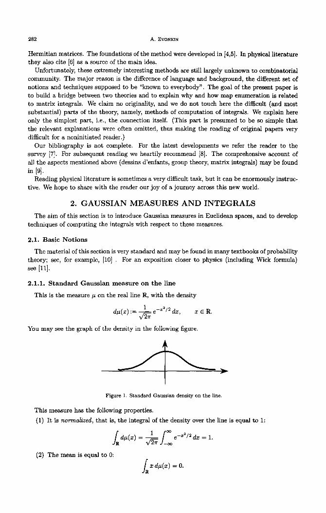
This is the measure /_J on the real line R, with the density

You may see the graph of the density in the following figure.

Figure 1. Standard Gaussian density on the line.

This measure has the following properties.

(1) It is normalized, that is, the integral of the density over the line is equal to 1:

J w dp(z) = -& J _I e-sa/2 dz = 1.

(2) The mean is equal to 0:

J zdp(z) = 0. B

Matrix Integrals and Map Enumeration 283

(3) The variance is equal to 1:

J “%&) = 1.

B

(4) The characteristic function (or Fourier transform) is

cp(t) := s, fez dp(x) = e-t2’2.

NOTATION 2.1. We will regularly use the following notation borrowed from physics: for any

measure p on X, and for any function f : X -+ R or f : X + @, we will denote by (f) the mean,

or average of f with respect to the measure ,LL:

(f) := s, f(x) 44x).

The measure p and the space X that are not explicitly mentioned in this notation will usually

be clear from the context. For example, the above formulae may be rewritten as

(1) = 1, (4 = 0, (x2) = 1, cp(t) := (eit”) = evt2j2.

2.1.2. General Gaussian measure on the line

This measure has the density

&L(X) := + e -((-42)/2~2 dx, x,m,a E lit, 0 > 0. ?Tcl

(1)

This measure is also normalized, and the mean, the variance, and the characteristic function are

as follows:

(x) = m, ((x - m)2) = 02, cp(t) := (eit”) = eimt-_(02ta/2)* (2)

REMARK 2.2. As is well known, a probabilistic distribution is uniquely determined by its char-

acteristic function. Hence, we could give the last formula for v(t) as a definition of a Gaussian

measure on the line.

2.1.3. Gaussian measure in IV

This measure will be the main object of our study. To introduce it we must start from its

characteristic function.

Let 2 = (xl, x2,. . . , xn) E IF. By (x, y) we denote the ordinary scalar product in lP, that is,

(2, y) := zlyl + * * . + xnyn.

DEFINITION 2.3. A measure p on lRn is called Gaussian, if its characteristic function has the

form

dtJ) dp(x) = exp i(m,t) - i(Ct,t)

where t, m E IP are vectors, and C = (~j) is a nonnegatively defined (n x n)-matrix of quadratic

form. Vector m is the mean vector of measure p, that is, (xi) = mi, and matrix C is its covariance

matti, that is, ((zi - mi)(xj - mj)) = r+.

REMARK 2.4. In what follows, for the sake of simplicity, we

mean m = 0, thus

p(t) = exp { --~CCt,t)}

consider only the case of the zero

(3)

284 A. ZVONK~N

and

(Xi) = 0, (ZiZj) = cij, i,j = 1,2 ,..., 71.

REMARK 2.5. The covariance matrix C may well be degenerate. Then the measure has no

density and is concentrated on a vector subspace of I&?. When C is nondegenerate, the measure

has density

&.4(z) = Const x exp { -;(Bz,z)} dz, (4)

where the matrix B = C-l. For this measure to be normalized, i.e., the measure of the whole

space Rn to be equal to 1, we should take the constant factor in the last formula equal to

Const = (2r)-n/2(det B)li2. (5)

All the above formulae (3)-(5) are consistent with the one-dimensional case (l),(2), where C =

(a2), B = (aV2), and Const = (27r)-1/2a-‘.

A Gaussian measure in R” is called standard if both B and C are identity matrices.

LEMMA 2.6. Let /J be a Gaussian measure in W”, and let A : IV’ --) R” be a linear operator.

Then A induces a measure Y in Rk which is also Gaussian.

PROOF. Let C be the covariance matrix of p, and let x, t E IFP, y, s E W”, and y = Ax. Then

where A* : R” -+ RF is the operator adjoint to A. What remains is to substitute A*s for t in

VP(t) = exp{-(1/2)(Ct, t)}, which g ives the covariance matrix of v equal to ACA*.

REMARK 2.7. In the above lemma, the dimension k may be less than n, equal to n, or greater

than n, and the operator A may be of an arbitrary rank.

2.2. Integrals of Polynomials and Wick Formula

A great part of the machinery of quantum physics consists of methods of calculating the

integrals with respect to a Gaussian measure (not necessarily in the finite dimensional case); see,

for example, [ll]. The goal of this section is to develop a technique for integration of polynomials.

2.2.1. Wick formula

Knowing that (xi) = 0, i = 1,. . . , n and (QX~) = cij, i, j = 1,. . . , n, one can easily compute

the integral of any polynomial of xi,. . . , x, of degree 2. What about higher degrees?

LEMMA 2.8. If f( ) x is a monomial of odd degree, then (f) = 0.

The following theorem reduces the integration of any polynomial of an even degree to that of

degree 2.

THEOREM 2.9. (Wick formula.) Let f~, f2,. . . , f2k be a set of linear functions (not necessarily

different,) of xl,. . . , xn. Then,

where the sum is taken over all the permutations plqlp2 . . . qk of the set of indices 1,2,. . . ,2k,

Such thatpr <p2 <*..<pk,pl <ql,...,pk <qk.

The number of summands on the right-hand side is equal to

(2k - l)!! := 1 x 3 x 5 x . -a x (2k - 1).


A partition of the set 1,2, . . . , 2k into couples (pi, qi) satisfying the conditions of the Wick formula

is called a Wick coupling.

EXAMPLE 2.10. As an example of application of the Wick formula let us compute a one-

dimensional integral

z4e-x2/2 dx = (x4) .

We have x4 = fl f2fsf4, where fl = f2 = f3 = f4 = x. Hence,

(flf2f3f4) = (flf2)(f3f4) + (flf3)(f2f4) + (flf4)(fif3).

Now each (fifj) = (z2) = 1; therefore the result is l2 + l2 + l2 = 3.

In the same way, we may find (x2”) = (2k - I)!!.

2.2.2. Wick formula: A sketch of the proof

In fact, the Wick formula is a very particular case of a formula well known in probability theory,

which expresses the moments of a probability distribution in terms of its semi-invariants. The

latter one, in its turn, is a “probabilistic interpretation” of the formula of logarithm of a power

series. For more details see, for example [12], Chapter 2 “Semi-invariants and combinatorics”.

We use the multi-index notation

a:=((Y1,...,cxn), Qi E N,

IaI:=cq+~~*+a,,

a! := al! x *. . x an!,

.p .= .p tan . l”‘n, where t = (tlr...,tn),

dlal f alQl f F := aty1 . . , &Em.

Let

f(t) = 1 + c Fta Ial> *

be the Taylor series for a function f(t) satisfying f (0) = 1, where

m aI*1 f

a = -3-F t=O.

Let the following be the Taylor series for log f(t):

log f(t) = c 2ta.

Ial> .

The formula below expresses the coefficients m, in terms of so.

PROPOSITION 2.11. The Taylor coefficients m, of a function f are expressed in terms of the Taylor coefficients sa of log f by the following formula:

Here pi are also multi-indices; the interior sum is taken over all ordered k-tuples of multi-indices

(but the factor l/k! ‘kills the order”).

286 A. ZVONK~N

REMARK 2.12. We skipped the condition of the analyticity

formula is also valid for formal power series.

PROPOSITION 2.13. Let p be a probability distribution in R”

Gaussian), and ^

of function f because the above

(an arbitrary one, not necessarily

p(t) = (ei@J)) = jRn ei@‘“) d/A(z),

its characteristic function. If cp is analytic in a neighborhood of 0, then all the moments m, := (xQ)

exist, and

cp(t) = 1 + c 3@)“.

l4>0

The coefficients s, of the series

log&) = c ?(it)“,

la1>0 cY.

are called semi-invariants of the distribution p, so the formula of Proposition 2.11 expresses the

moments of a probability distribution in terms of its semi-invariants.

The formulae and computations involving semi-invariants are often much simpler than those

involving moments. A Gaussian distribution is a striking example of this phenomenon, as for the

characteristic function (3), its logarithm is no more an infinite series but a quadratic polynomial

logcp(t) = -+t,t),

so s, # 0 implies Ial = 2, and for such an Q we have s, = m, = ~j (here ai = cyj = 1 if i # j,

and ai = 2 if i = j, while all the other components of the multi-index (Y are equal to 0).

Return now to the Wick formula. Let y1 = fi(z), . . . , YZk = f‘&(X). According to Lemma 2.6

vector (yl, . . . , y2k) has a Gaussian distribution, and our goal is to compute, for this distribution,

the moment (~1.. . y2/2k) which corresponds to the multi-index o = (1, 1, . . . , 1). Now we may

apply the formula of Proposition 2.11 and to split cr into the sums of multi-indices pi, of which

survive only those of the form (0,. . . ,O, l,O, . . . ,O, l,O, . . . , 0), having only two nonzero entries.

The Wick formula is proved.

3. THE SPACE OF HERMITIAN MATRICES

In this section, we consider a very special case of the previous construction, namely, a Gaussian

measure on the space of Hermitian matrices.

3.1. Definitions and Notation

Let H = (hij) denote an Hermitian (N x N)-matrix; that is, its entries are complex numbers:

h, E @ and hij = &, where the bar denotes the complex conjugation. We denote by ?f~ the

space off all such matrices.

Every Hermitian matrix may be described by N2 real parameters: xii = hii E R, i = 1,. . . , N

for diagonal entries, and xij = Re(hij), yij = Im(hij), 1 5 i < j 5 N for over-diagonal entries

(the under-diagonal entries being determined by the over-diagonal ones via complex conjugation).

Thus, the space ‘FIN is isomorphic to the Euclidean space RN’. We introduce the ordinary

Lebesgue measure in %N:

dv(H) := fi dxii I-J dxij dyij. i=l i<j

In principle, the space ‘HN 2 RN2 does not differ from any other Euclidean space of the same

dimension. But some of the characteristics of the Gaussian measure on it will be expressed in


terms of matrix operations. In order to introduce a Gaussian density in the form (4), we need a

nondegenerate quadratic form in %N. We take as such a form the following one: tr(H2).

Let us see how this form looks in the coordinates zij, yij. A term (.)ik of H2 is equal to

c3N,i hijhjk; h ence, a diagonal term (.)ii is equal to C& hijhji, and hence, the trace of H2 is

equal to

N N N N

tr (Hz) = C hijhji = 1 hijG = C XZ + C (me + yfj) = C xfi + 2 C (xfj + y,j:\ . i,j=l i,j=l i=l i#j i=l i<j

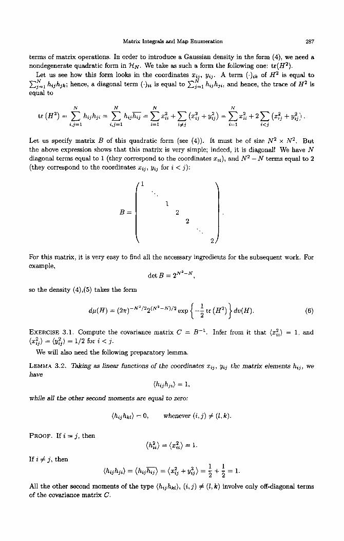
Let us specify matrix B of this quadratic form (see (4)). It must be of size N2 x N2. But

the above expression shows that this matrix is very simple; indeed, it is diagonal! We have N

diagonal terms equal to 1 (they correspond to the coordinates Q), and N2 - N terms equal to 2

(they correspond to the coordinates zij, yij for i < j):

B=

1

2

2

2

For this matrix, it is very easy to find all the necessary ingredients for the subsequent work. For

example,

det B = 2N2-N,

so the density (4),(5) takes the form

&(H) = (2,+-N2/22(N2-W exp { -$ tr (H’)}dv(H). (f-3

EXERCISE 3.1. Compute the covariance matrix C = B-l. Infer from it that {zfi) = 1, and

(x2) = (y$) = l/2 for i < j.

We will also need the following preparatory lemma.

LEMMA 3.2. Taking aa linear functions of the coordinates zij, yij the matrix elements hij, we

have

(hijhj,) = 1,

while al1 the other second moments are equal to zero:

(hijhd = 0, whenever (i, j) # (I, k).

PROOF. If i = j, then

(hyi) = (xfi) = 1.

If i # j, then

(hijhji) = (hijhij) = (~z + Yi”j) = i + f = 1.

All the other second moments of the type (hijhkl), (i, j) # (I, k) involve only off-diagonal terms

of the covariance matrix C.

288 A. ZVONKIN

3.2. An Example

Now, we are ready to try the efficiency of the developed techniques for computing an integral of some polynomial. Let us consider the following one: tr(H2”). It is a polynomial of degree 2k of N2 variables h,j, which are, in their turn, linear functions of xij, 9i.j. More precisely,

tr (H2”) = C hili2hi2i, + . . hi2,_,i2,hi,,i, 7 (7)

where the sum is taken over all N2k combinations of indices ii, iz, . . . , i2k. Consider the integral

(tr (H2k)).

In order to compute it, we must apply the Wick formula to expression (7). Let us look at how it works in a particular case.

EXAMPLE 3.3. Let k = 4, so we deal with the sum of the Ns products of the form

h. h h. h. h, h. h, h. 2122 2223 2314 2425 25% %27 27% @al

Let us choose an arbitrary Wick coupling (out of 7!! = 105 ones). For example, let us couple hiliz

with hi4iS; hiZi3 with hiSi6; hi3i4 with hisi,; and hiSi, with hiTie; in other words, let US consider the product

~~~~~~~~~~~~~~~~~~~~~~~~~~~~~~~~~~~~~~~~~~~~~~~~~ (3)

Recalling Lemma 3.2, we see that each factor of this product has quite good chances to be equal to 0 (and then the whole product will become 0). In order for the product to be nonzero, we need all of its factors to be equal to 1 (then the product itself is also equal to 1). And for that,

we must impose rather restrictive conditions on indices (see once more Lemma 3.2):

(hili2hi4<5) = 1 w ii = is, i2 = id,

(hi,i,hi,i,) = 1 w i2 = i6, is = is,

(hi3i4hi8il) = 1 u i3 = il, i4 = ig,

(hi6i7hili8) = 1 C is = is, ir = ir.

Finally, we have the following “chains of equalities”:

il = i5 = i3 = il,

i2=i4=i8=i6=i2,

i7 = i7,

which gives us N3 possible combinations of indices (the indices il, is, and i7 may be chosen arbitrarily, while the values of all the other indices are determined by this choice). This fact is usually expressed by saying that the contribution of the coupling (8) is equal to N3.

In general (for an arbitrary k, and for an arbitrary coupling), the contribution is equal to NV,

where V is the number of ‘<free indices”.

It seems that the question is more or less settled. But the most interesting part of the story only

begins, because the above equalities among indices have a fascinating geometric interpretation.

4. MAPS

4.1. Graphs, Surfaces and Maps: Basic Notions

Basic facts concerning the combinatorics of maps may be found, for example, in [13].


Figure 2. A graph

4.1.1. Graphs

We accept graphs with loops and multiple edges, as well as graphs with vertices of degree 1

and 2 (see Figure 2). But usually we will only consider connected graphs.

4.1.2. Surfaces

We will consider compact oriented 2-dimensional manifolds without boundary. From now on

we will simply use the word surface to denote such an object. The genus of a surface is the

number g 2 0 of “holes” in it, or the number of “handles”; see Figure 3.

Figure 3. Surfaces of genus g = 0, 1,2.

The surfaces are classified according to their genera: every surface has genus, which is a

nonnegative integer, and there is only one, up to a homeomorphism surface of any given genus.

4.1.3. Maps

A map is a graph drawn on a surface. The difference between the notion of a graph and that

of a map is rather subtle and does not strike one’s eye. The reason is that whenever we deal

with a graph, we usually draw it. But the mere fact of drawing a graph provides it with some

additional mathematical structure.

Let us be more precise.

DEFINITION 4.1. A map is a graph which is “drawn” on (imbedded into) a surface in such a way

that:

* the edges do not intersect;

o if we “cut” the surface along the edges, we get a disjoint union of sets which are homeo-

morphic to an open disk (these sets are called faces of the map).

The second condition implies the connectedness of the graph. It is important to notice that

the graph itself does not have any faces, but only vertices and edges. The degree of a vertex is

the number of edges incident to it (a loop incident to a vertex is counted twice). The degree of a

face is the number of its boundary edges (an edge may be adjacent to a face “from both sides”;

then it is counted twice).

PROPOSITION 4.2. The following quantity, which is called the Euler characteristic of a map,

x = #(vertices) - #(edges) + #(faces) = 2 - 29,

does not depend on the map itself but only on the genus of the surface on which it is drawn.

290 A. ZVONKIN

REMARK 4.3. Sometimes it is necessary to consider nonconnected maps. In such a case, the maps

are considered as drawn not on a single surface, but on several disjoint surfaces (one surface for

each component). The Euler characteristic is additive, that is, the Euler characteristic of the

whole map is the sum of the Euler characteristics of its components (because the numbers of

vertices, edges, and faces are additive), while the genus is not additive.

4.2. Examples

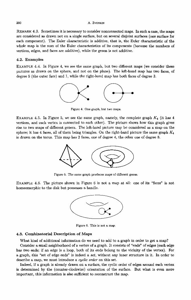
EXAMPLE 4.4. In Figure 4, we see the same graph, but two different maps (we consider these

pictures as drawn on the sphere, and not on the plane). The left-hand map has two faces, of

degree 5 (the outer face) and 1, while the right-hand map has both faces of degree 3.

Figure 4. One graph, but two maps.

EXAMPLE 4.5. In Figure 5, we see the same graph, namely, the complete graph K4 (it has 4

vertices, and each vertex is connected to each other). The picture shows how this graph gives

rise to two maps of different genera. The left-hand picture may be considered as a map on the

sphere; it has 4 faces, all of them being triangles. On the right-hand picture the same graph K4

is drawn on the torus. This map has 2 faces, one of degree 4, the other one of degree 8.

Figure 5. The same graph produces maps of different genus.

EXAMPLE 4.6. The picture shown in Figure 6 is not a map at all: one of its “faces” is not

homeomorphic to the disk but possesses a handle.

Figure 6. This is not a map.

4.3. Combinatorial Description of Maps

What kind of additional information do we need to add to a graph in order to get a map?

Consider a small neighborhood of a vertex of a graph. It consists of “ends” of edges (each edge

has two ends; if an edge is a loop, both of its ends belong to the vicinity of the vertex). For

a graph, this “set of edge ends” is indeed a set, without any inner structure in it. In order to

describe a map, we must introduce a cyclic order on this set.

Indeed, if a graph is already drawn on a surface, the cyclic order of edges around each vertex

is determined by the (counter-clockwise) orientation of the surface. But what is even more

important, this information is also sufficient to reconstruct the map.


PROPOSITION 4.7. Any given cyclic order of the ends of edges of a graph around each vertex (chosen arbitrarily and independently at each vertex) uniquely determines the imbedding of the

graph into a surface, i.e., a map.

This result is usually attributed to Edmonds [14], though according to certain authors it goes

back to Heffter [15] or even to Hamilton [16]. Anyway, it is now widely known to combinatorialists

working with maps. Instead of giving a formal proof of the proposition, we give a simple geometric

construction which explains how the map is reconstructed from the cyclic orders of edges around

vertices.

Let us represent an edge as a “two-way” street.

\

>

Figure 7. A two-way street.

Let us represent a vertex as a crossroad made as a “roundabout” (Figure 8). This geometric

image of a roundabout corresponds nicely to the formal notion of cyclic order of edges around a

vertex. Now, let us move through this city, always respecting the following rule: hating come to

a crossroad, leave it by the first street to your right.

Figure 8. A “roundabout” crossroad

Then all possible routes form a set of disjoint cycles.

Figure 9. A face.

We may consider these cycles as faces of a map. We may just call them faces, in a purely

formal manner, filling them by open polygonal sets. Note, that the streets at each crossroad are oriented counter-clockwise, but the boundaries of faces are oriented clockwise.

This construction is often called a “ribbon graph”, or a “fat-graph”.

REMARK 4.8. For the graph shown in Figure 6, the cyclic order of the edges around vertices is

also prescribed by the imbedding. But when we reconstruct the map structure from this cyclic

order, we must glue a simple pentagon as its outer face. The map thus becomes of genus zero: the handle has appeared illegally.

292 A. ZVONKIN

In a dual approach, we may start from a number of faces, that is, polygons with their boundaries oriented clockwise, with the total number of edges being even, and then glue the edges pair-wise in an arbitrary (but connected) way, always respecting the rule that the Bsrows glued together must point in opposite directions, as in Figure 10. Then the cyclic order of edges around a vertex is determined by the rule: the next edge is the one that we may access to by the interior of the face.

Figure 10. Gluing of faces.

The number of cyclic orders of edges of a graph at a vertex v of degree d, is (d, - l)!. Therefore, the total number of edge orderings of the graph is equal to n(du - l)!, where the product is taken over the set of vertices, and every such ordering leads to a map. There exist many unusual imbeddings even for well-known graphs. The reader may entertain him or herself by trying to imbed, for example, the graph of the cube into the torus (in a regular way, so that all the faces be hexagons), or the graph of the icosahedron into the surface of genus 4 (also regularly, so that all the faces be pentagons).

5. ONE FACE MAPS

5.1. An Enumeration Problem

Consider a polygon with 2k sides. This polygon will serve as the only face of the maps we are going to construct. Orient the polygon perimeter clockwise, and label its vertices by labels . . z1,22,. . . , &?k. Now, let us split the sides of the polygon into pairs in an arbitrary way, and glue together the sides belonging to each pair, always respecting the rule “end to the head”. What we get is a map.

There are (2k - l)!! ways of splitting the set of the labeled edges into pairs. (Indeed, couple the first edge with any of the other 2k - 1 ones; than couple the first “nonappointed” edge to any one of the 2k - 3 edges that left, etc.). Hence there are (2k - l)!! corresponding maps. Our goal is to enumerate them according to their genus. It is easy to see that the maximal genus is equal to [k/2], where the square brackets denote the integer part. So we are looking for the numbers

sg (k) : = #(gluings of 2k-gon of genus g), c e,(k) = (2k - l)!!. g=o

This problem has all the attributes of a worthy problem: it is beautiful, difficult, and important. The answer for the genus zero has been well known for a long time: it is given by Catalan numbers,

co(k) = cr, = j-& “k” . 0

(9)

Some preliminary results for arbitrary genus were obtained in [17]. The problem was completely solved in [18].

Let us see how to determine the genus of a map in question. In order to compute its Euler characteristic, we must know the number of vertices V, the number of edges E, and the number of faces F. The number of faces is the easiest to found: our map has only one face by construction,


namely, the polygon itself; so F = 1. As to the number of edges, it is equal to E = k, because

the original polygon had 2k sides, and they were glued together in pairs. The only unknown

parameter is the number V of vertices. We have

x=V-E+F=V-k+1=2-2g,

hence,

V=k+l-2g.

Let us look how to determine V in a particular example.

EXAMPLE 5.1. Consider a polygon with 8 sides, and glue its sides in pairs as is shown in Figure 11.

Figure 11. A polygon whose sides are glued together in pairs

We remind to the reader that the arrows must be glued together in the opposite directions. The

fact that the side labeled iliz is glued to the one labeled idis, means that the polygon vertex ir

is identified with is, as well as is is identified with id. We express this by writing

il = is, i2 = i4.

In the same way, the side i& is glued to isis, hence,

i2 = i6, i3 = is,

and the two remaining identifications give us

i3 = il, i4 = ig, i6 = is, i7 = i7.

Finally, we see that the 8 original vertices of the polygon are identified in the following way (thus,

producing 3 vertices of the corresponding map):

il = is = is = il,

i2 = i4 = is = is = i.2,

i7 = i7.

We hope that by now the reader has recognized the equalities of Example 3.3. This leads to a geometric interpretation of the Wick coupling described in Section 3.2.

294 A. ZVONKIN

5.2. Back to Gaussian Integrals

We will “graphically represent” the integral of tr(Hzk) by a polygon with 2k sides whose vertices are labeled by ii, iz, . . . , i2k clockwise. The cyclic structure of indices in (7) is reflected in the cyclic arrangement of labels around the polygon. Each of (2k - l)!! Wick couplings is represented by one of the (2k - l)!! gluings of the sides of the polygon, that is, by the corresponding one-face map. (In the language of physics, one would say that this map serves as a Feynman diagram for our integral.) The number V of free indices of a Wick coupling is equal to the number V = k + 1 - 2g of vertices of the corresponding map. The contribution of a coupling (map, diagram, whatever) into the integral is equal to NV.

We have established the following theorem [18].

THEOREM 5.2. Let f(k,N) be

f(k, N) := (tr (H2”)) = k, tr (H2”) dP(H),

where the integral is taken over the space ?iN of Hermitian (N x N)-matrices with respect to the Gaussian measure (6). Then

[k/21 f(k, N) = c ,S(k)Nk+‘-2g = N”+’

g=o [?&g(k) (,)g, g=o

where eg(k) is the number of labeled one-face maps of genus g with k edges.

REMARK 5.3. The function f(k, N) may be considered as a kind of a generating function for the numbers am, where the role of a formal parameter is played by the quantity l/N2.

5.3. Results and Discussion

We have explained only a very small part of the paper [18], where the method of matrix integrals was independently rediscovered. Now, one must compute the integral, which is not at all an easy task:

The next step is to extract from the above formula an information concerning the numbers e,(k). The final result takes the form of a recurrent relation

- 2 +1sg(k 4k

- - - &g(k) = - 1) + (k 1)(2k 1)(2k

k+l 3)E 9 _-l(k _ 2) 7

with the boundary conditions

Eg(O) = I

1, if g = 0,

0, otherwise.

The table of values of .sg( k) may be found in [18]. Relations (10) are so simple that one is tempted to look for a purely combinatorial proof,

without matrix integrals. The first such proof, using characters of the symmetric group, was given in [19]. It was still very complicated. A considerable simplification is achieved in [20]. But a convincing purely geometrical proof still does not exist.

The enumerative result for eg(k) in [18] has only served as a combinatorial lemma in a study of a much more complicated object, namely, the moduli space of algebraic curves. The method of computation of its (virtual) Euler characteristic based on this lemma was later considerably simplified by Kontsevich [21] who reduced the problem to the computation of a one-dimensional Gaussian integral. In cartographic terms, the main result of [21] may be formulated ss follows.


For any map m let V(m) and E(m) denote the number of its vertices and edges, respectively.

Let M, be the set of maps such that the degree of each vertex is at least 3, and E(m) - V(m) = n

(we no longer demand the number of faces to be equal to one). Note, that this set M, is finite.

THEOREM 5.4. The following formula is valid:

c wvy = &+1

mEM, Put (ml n(n + 1) ’

where IAut(m)I is an order of the automorphism group of the map m, and B,+l is a Bernoulli

number.

6. ONE MORE INTEGRAL

Let us consider the following more complicated integral:

Z(t,N):= (exp{-$tr(H’)}), (11)

(historically, this integral was studied earlier than the previous one, see [4,5]). On the one hand,

tr(H4) is simpler than tr(H2”); on the other hand, we have here an exponential function, while

we only know how to integrate polynomials.

REMARK 6.1. Integral (11) is not trivial even in the one-dimensional case:

Z(t) = & _I &z2/2)-ts* dx. .I We see that the latter integral converges for all t > 0 and diverges for all t < 0. Hence, it cannot be analytic at t = 0. In physics, this reasoning is called “Dyson’s argument”. The integral may

be expressed in terms of Bessel functions.

6.1. Perturbative Series

If we must deal with the exponential function but are only able to integrate polynomials, then

it is clear what to do: we must first expand the exponential function into a power series:

exp {-k tr (H4)} = C $ (-$)” (tr (H4))“. ?I>0

And now we must struggle only against (tr(H4))“. We have

tr (H4) = 2 hijhjkhklhliy i,j,kJ=l

hence,

where the sum is taken over all the N4” possible combinations of indices. And now we must

apply the Wick formula to this incredibly cumbersome expression! Feynman diagrams are indeed

an invaluable tool for overcoming many-storeyed indices, i.e., to present them in a geometric way.

296 A. ZVONKIN

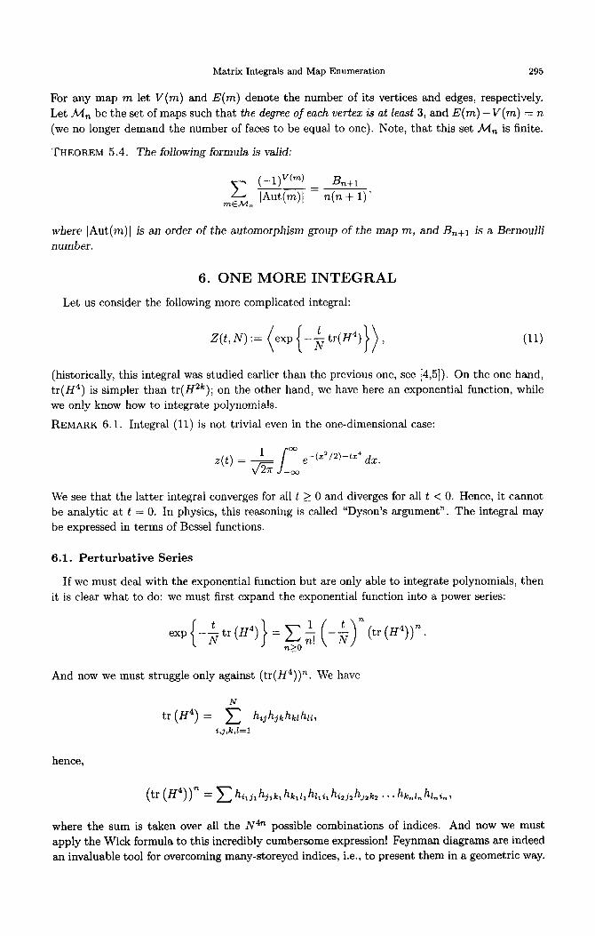
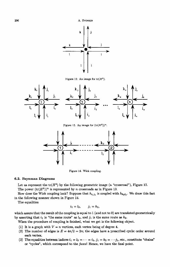
Figure 12. An image for tr(H4)

Figure 13. An image for (tr(If4))”

<A lL______<3-i ll- +fp+ - - - - - - -qyf-* Figure 14. Wick coupling.

6.2. Feynman Diagrams

Let us represent the tr(H4) by the following geometric image (a “crossroad”), Figure 12. The power (tr(H4))” is represented by n crossroads as in Figure 13. How does the Wick coupling look? Suppose that hi,j, is coupled with hk212. We draw this fact

in the following manner shown in Figure 14.

The equalities ii = 12, jr = kz,

which assure that the result of the coupling is equal to 1 (and not to 0) are translated geometrically by asserting that ir is “the same route” as 12, and jr is the same route as kz.

When the procedure of coupling is finished, what we get is the following object.

(1) (2)

(3)

It is a graph with V = n vertices, each vertex being of degree 4. The number of edges is E = 4n/2 = 2n; the edges have a prescribed cyclic order around each vertex. The equalities between indices ii = 12 = . . - = il, jl = k2 = . e . jl, etc., constitute “chains” or “cycles”, which correspond to the faces! Hence, we have the final point.


(4) The contribution of a diagram into the integral (11) is equal to NF, where F is the number

of faces of the diagram.

Having in mind that the Euler characteristic is

we get the following result:

z(t,N) = c 5 (-$)” c Nnfx = c -$(-t)” c NX, n>O 7L>O

where the internal sum is taken over all the diagrams (couplings).

But this is not yet the result for which we are looking.

6.3. Logarithm

We have missed a very important point: our diagrams do not have to be connected. Quite

on the contrary: we must consider all the possible matchings, disconnected ones included. (We

tried to avoid the term “map” for this object on purpose.) In order to find a more interesting

combinatorial result, we must yet perform four more operations.

(1) Take the logarithm of Z(t, N). This operation is very well known in combinatorics; see, for

example, [22]. If one has an ezponelztial generating function for a class of labeled objects, then

its logarithm is the generating function of the connected objects of the same type.

The word “exponential” means “with n! in the denominator”. The term “labeled” should be

explained at more length. But we will limit ourselves to a single remark. One may consider

the objects (such as graphs) with additional structures (such as cyclic orders of edges around

vertices) and with some properties imposed (such as the prescribed vertex degrees). But, one

must be careful: a property has a legal right to be imposed when it is valid for an object if and only ,if it is valid for all its connected components. For example, the property:

every vertex of a graph is colored in one of k colors

is acceptable; on the contrary, the property:

every vertex of a graph is colored in one of k colors, and all k colors are used

is notf good, because it may be valid for a graph as a whole but not valid for some of its components.

See the discussion of this subtle point in [23].

Concerning the proof, we may once more use the formula for the logarithm of a power series of

Proposition 2.11, with a slight change of the interpretation. First, we must specialize the formula

from multi-indices to simple (one-dimensional) indices. Second, we must generalize the notion of “coefficients” (sa or m,), considering them as “weights” taking values in a ring. The weight of

an object must be the product of the weights of its connected components.

In our case, the weight of a diagram is equal to NX, and the multiplicativity of this weight is

implied by the additivity of the Euler characteristic x, see Remark 4.3. Thus, finally,

logZ(t, N) = c $(-t)” 1 N2-2g, l+l

where the second sum this time is taken over all the connected diagrams, and g is the genus of a

diagram.

(2) Let us now divide the result by N2, in order to have weights of the form Nm29.

298 A. ZVONKIN

(3) The third operation is to change the sign preceding the whole thing, that is, to take the “minus logarithm”. This operation is not very meaningful mathematically, but it is meaningful

from the physical point of view. As one physicist has put it, “Partition function does not have its own physical meaning, but its logarithm has the meaning of energy”. Function Z(t, N) obviously

has the meaning of a partition function (see discussion below), i.e., it is a “sum” (rather an

integral) of the exponents of “minus energy”. This is yet another facet of the logarithm of a

power series.

(4) The last operation is the changing of the summation order, to collect the diagrams of the

same genus. Finally, we get the following theorem (see [4,5]).

THEOREM 6.2. Let E(t,N) be

E(t,N) := - $log .z(t,IV) = -$ log ( I

exp -$tr(H’)}).

Then,

E(t) N) = c ( gg E,(t), 910

where

J%(t) = - c &)“Kg(n) n>l

and K,(n) is the number of connected diagrams of genus g with n vertices.

Once again l/N2 plays the role of a formal parameter in the genus expansion.

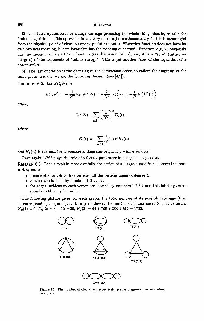
REMARK 6.3. Let us explain more carefully the notion of a diagram used in the above theorem.

A diagram is:

l a connected graph with n vertices, all the vertices being of degree 4,

l vertices are labeled by numbers 1,2,. . . , n,

l the edges incident to each vertex are labeled by numbers 1,2,3,4 and this labeling corresponds to their cyclic order.

The following picture gives, for each graph, the total number of its possible labelings (that

is, corresponding diagrams), and, in parentheses, the number of planar ones. So, for example,

Ko(l) = 2, KC,(~) = 4 + 32 = 36, X0(3) = 64 + 768 + 384 + 512 = 1728.

3 (2) 24 (4) 72 (32)

2592 (768)

Figure 15. The number of diagrams (respectively, planar diagrams) corresponding to a graph.


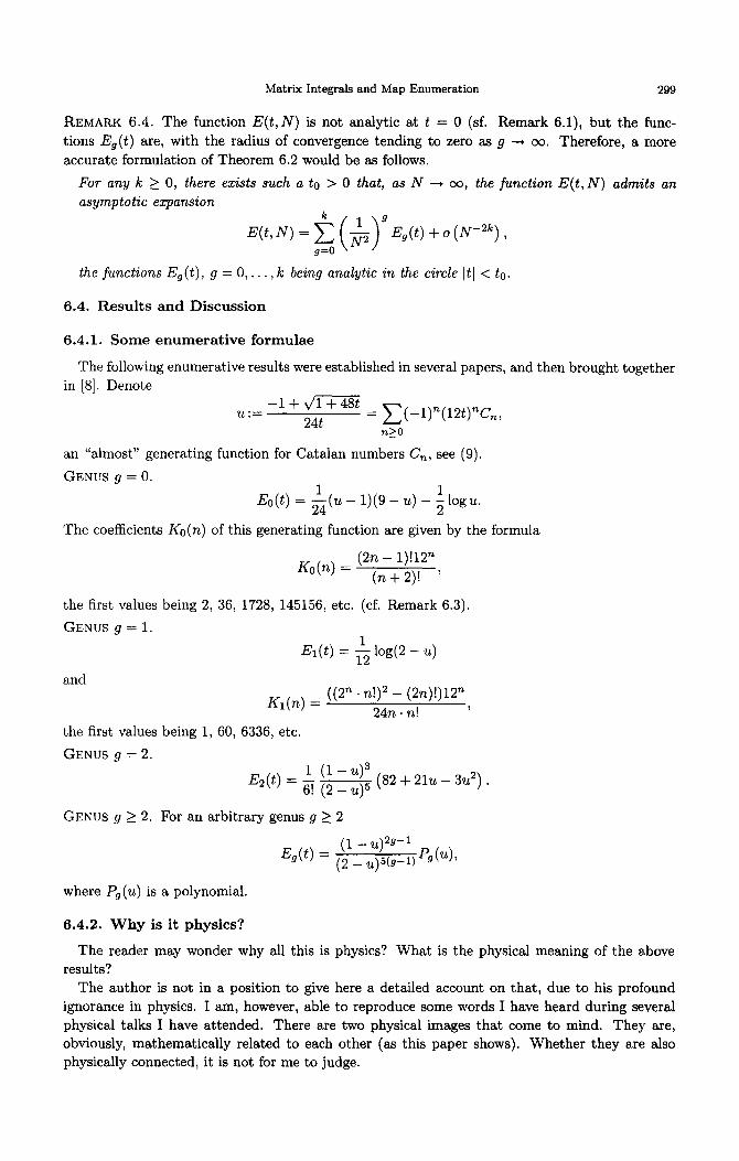
REMARK 6.4. The function E(t,N) is not analytic at t = 0 (sf. Remark 6.1), but the func-

tions E,(t) are, with the radius of convergence tending to zero as g -+ 00. Therefore, a more

accurate formulation of Theorem 6.2 would be as follows.

For any k 1 0, there asymptotic expansion

exists such a to > 0 that, as N 4 00, the function E(t, N) admits an

E(t, N) = & ($)’ E,(t) + o (N-2k) , g=o

the functions E,(t), g = ,..., 0 k being analytic in the circle ItI < to.

6.4. Results and Discussion

6.4.1. Some enumerative formulae

The following enumerative results were established in several papers, and then brought together

in 181. Denote / 1

-1+diTx u:=

24t = C(-1)“(12t)nC,,

n>O

an “almost” generating function for Catalan numbers C,, see (9).

GENIJS g = 0.

Eo(t) = &(u - 1)(9 - U) - f logu.

The coefficients J&(n) of this generating function are given by the formula

Ko(n) = Pn - lwn (n+2)! ’

the first values being 2, 36, 1728, 145156, etc. (cf. Remark 6.3).

GENCJS g = 1.

and

El(t) = & log(2 - u)

. n!)2 - (2n)!)12n Kl(n) = ((2” 24n . n! ,

the first values being 1, 60, 6336, etc.

GENUS g = 2.

E2(t) = 1 (1 (82 + 21~ - 3u2) . 6! (2 - u)~

GENUS g 2 2. For an arbitrary genus g 2 2

-G(t) = (1 - 42g-1 pg(u)

(2 - q(P-1) ’

where Pg(u) is a polynomial.

6.4.2. Why is it physics?

The reader may wonder why all this is physics ? What is the physical meaning of the above

results?

The author is not in a position to give here a detailed account on that, due to his profound

ignorance in physics. I am, however, able to reproduce some words I have heard during several

physical talks I have attended. There are two physical images that come to mind. They are,

obviously, mathematically related to each other (as this paper shows). Whether they are also

physically connected, it is not for me to judge.

300 A. ZVONKIN

String Theory

In classical mechanics, a point particle that moves from A to B chooses a trajectory o(t) that

minimizes the functional of action S[Z]. In quantum mechanics (more exactly, in Feynman path

integrals approach), a particle moves from A to B along all possible trajectories, the contribution

of each trajectory into the “amplitude of probability” being e-(i’ti)slZl. In order to compute

the amplitude (and other physical quantities), one must evaluate an integral over the space

of all possible trajectories. One of the techniques of such a computation consists in replacing

trajectories by broken lines, thus reducing the problem to a finite-dimensional integration. If in

the process of its evolution in time the particle breaks down into two, and/or two particles collide

and form one particle, the space of trajectories becomes more complicated (see Figure 16).

yB /a+’ A A

A

Figure 16. Feynman paths and their discrete approximations.

In the string theory approach, a particle is no more point-like, but is a small circle (“string”).

As this circle evolves in time, a two-dimensional surface appears, which serves as an analog of a

trajectory. The process of breaking down/colliding is described by the addition of a new handle

to the surface (Figure 17).

Figure 17. Evolution of a string in time.

The path integrals are now replaced by integrals over the space of two-dimensional surfaces.

There are two main strategies of reducing these integrals to finite dimensional ones (miraculously,

both strategies lead to the same physical results). One consists in considering a surface as a

complex algebraic curve. It is well known that the space of complex algebraic curves (or, more

accurately, the space of parameters describing them, the so-called moduli space of curves) is

finite-dimensional, its complex dimension being 3g - 3 for g 2 2, 1 for g = 1, and 0 for g = 0.

Thus, instead of integrating over the space of surfaces, one may integrate over the moduli space.

Another approach consists in replacing a surface by its discrete approximation, that is, by a

map! Thus, enumeration of maps becomes relevant to this physical model, being an approximate

computation of Feynman path integrals over the space of “two-dimensional paths”. Many physical

papers cited in our bibliography compute some parameters of physical interest, such as, for

example, “string susceptibility”.

Quantum Field Models

A general scheme according to which the models of quantum fields theory are constructed is

as follows. There is a space X that is a model of the Universe. Fields are functions f : X --t Y


taking values in a space Y. There is a measure on the space F of all fields. The general form of

the measure is

exp{-(quadratic functional off) - (interaction term)},

where interaction term is nonquadratic. When there is no interaction, the measure becomes

Gaussian (as it becomes exponent of a quadratic term), and it is called “free field”. The inter-

action term may also depend on some parameters. Then we must integrate with respect to this

measure, and study the dependence of the results on parameters.

Obviously, the matrix model considered above has all the ingredients of this general scheme.

The role of the space Y is played by tiN, the space of Hermitian matrices. The free field and

the corresponding Gaussian measure are described by the quadratic functional (l/2) tr(H2). The

interaction t,erm is (t/N) tr(H4). Th e most unusual part of the story is, however, the space X:

in our model the Universe consists of one point!

To my mind, this feature of the model shows in a very striking way the level of mathematical

nontriviality of modern theoretical physics. Even the simplest imaginable models may 1ea.d to

very complicated mathematical considerations.

7. FURTHER RESULTS, QUESTIONS, AND DISCUSSION

7.1. A Variety of Integrals

There are many other matrix integrals, computed or otherwise studied in a vast literature. It

would

(1)

(2)

(3)

(4)

(5)

(6)

(7)

(8)

be very difficult to explain all of them in full detail, but it is worth making a brief survey.

Replacing H4 by H3 gives rise to the enumeration of triangulations (or, dually, of trivalent

graphs); see, for example, [24].

More complicated “trace polynomials” of the form ni(tr(Hki))ma are integrated in [25].

These enumerate maps with prescribed face degrees.

Considering an “interaction potential” of the form

U(H):=H+;H2+;H3+...= - log(1 - H),

is used to enumerate maps with arbitrary vertex degrees, see [26].

Considering a Gaussian measure with nonzero mean may help to enumerate maps without

loops (Kszakov, private communication).

Integrals over the space of real symmetric matrices are related to maps on nonoriented

surfaces (see forthcoming works of Goulden).

The %wo-matrix” model is very interesting physically (but much more complicated com-

putationally), see [5]. The Gaussian measure in ‘HN x XN is introduced by means of the

quadratic form

tr (Hf -t Hi - 2cH1 Hz) .

While considering Feynman diagrams for this measure, we must assign to each vertex

either HI or Hz, the contribution of the diagram depending on this assignment. Thus, the

diagrams are configurations of the Ising model on the graph in question.

While the two-matrix model is solved, its direct generalization, the n-matrix model, is

not.

A kind of a Potts model suggested by Kazanov is related in [27] to the problem of enu-

merating “meanders”. This model involves 2q matrices, q being one of the parameters of

the model. For later development, see [28].

In [29], the first attack is launched against the most intriguing (but undoubtedly. very

difficult) problem of enumerating maps according to both the set of vertex degrees and

the set of face degrees.

302

6-J)

(10)

A. ZVONKIN

The most famous recent application of the method of matrix integrals is [30]. Kontse-

vich has proved a conjecture of Witten, and has shown, among other things, that some

generating functions for maps satisfy higher analogs of the Korteweg-de Vries equation.

Some additional references: for various methods of computation of matrix integrals,

see [31-331; for experimental numerical results, see [34]; for various recent developments,

see [7,35-371.

7.2. First Glimpses of the Computation of Integrals

The fundamental observation is that the density (6), as well as all the functions of H we

would like to integrate, are unitary invariant. This means that we may introduce the so-called

“polar coordinates” in the space tiN, representing each matrix H E tiN by a pair (U, A), where

U E U(N) is a unitary matrix, A is a diagonal matrix, and

H = UN-I. (12)

Then the density and all the integrands depend only on A and do not depend on U.

These “coordinates” are not coordinates properly speaking, as the representation (12) is am-

biguous. The matrix A is determined to within permutation of its diagonal entries Xi, i = 1,. . . , N

(and the corresponding permutation of the columns of U), and the matrix U, in the case of all Xi

different (the opposite case has measure 0), to within multiplication by a diagonal matrix of the

form

(@ eirpz . . . e,,.).

This ambiguity is responsible for the factor 1/((27rtN . N!) in the formula below.

The following proposition asserts two major facts: first, that we may “integrate out” the

unitary part, and second, that the Jacobian of this change of variables is equal to the square of

the Vandermonde determinant.

PROPOSITION 7.1. Let a function f(H) be unitary invariant. Then,

I ‘Hi-l fcH) hdH) = (24: , N! vol(U(N)) lRN f(A) n(xi - U2 %A),

i<j

where vol(U(N)) is the volume of the unitary group, and

dy(A) := (27r)-N’2 exp

is the standard Gaussian measure in RN.

The volume of the unitary group is induced by the metrics of its imbedding as a N2-dimensional

surface into the space of complex (N x N)-matrices, and this latter space is considered as W2NZ. This volume was calculated many times, for different purposes. It is equal to

vol(U(N)) = (“$;;,““. kl ’

The functions to integrate are: f(A) = tr(A2”) = C Xfk for one of the models considered above;

f(A) = exp{-(t/N) tr(A4)} = exp(-(t/N) C Xf) for the other. But we would propose, to begin

with, to compute the integral of the function f(A) E 1. The result is known in advance, of course:


it is equal to 1 (the measure is normalized!). Being compared to the formula for the volume of

U(N), this result is equivalent to the following identity:

Sn RN (Xi - Xj)2dv(A) = fi k!.

Z<j k=l

The right-hand side suggests some (yet unknown) combinatorial meaning. The left-hand side

contains an integral with respect to the standard Gaussian measure in RN, of a polynomial that

seems to be specially prepared for an application of the Wick formula, as it is already split

into linear factors. However, the only way known to the author to prove this identity is not

combinatorial: it involves Hermite polynomials.

7.3. Some Questions, Not Necessarily Open

(1)

(‘4

(3)

Witten [38] characterizes the works [39-411 as a “spectacular success”. All these papers

deal with an asymptotic enumeration of maps of arbitrary genus. The results obtained

seem to be very similar to those obtained in [42], which also treats maps of arbitrary genus

(this last paper is cited in [40]). The question is, what are the physical implications of the

works of Bender and his co-authors on asymptotic map enumeration?

A very general nature of Proposition 2.11 suggests paying a closer attention at a general

theory of integration of power series with respect to various measures. A most obvious ob-

stacle is the theorem of Marcinkiewicz (see, for example, [43]) stating that if the logarithm

of the characteristic function of a probabilistic distribution is a polynomial, then it is a

quadratic polynomial, and the distribution is Gaussian. So, in a case other than Gaussian,

we must deal with an infinite series. Or maybe it is worth considering a convolution not

with a probabilistic measure but with an arbitrary function which is an inverse Fourier

transform of a polynomial (such as the Airy function). As an example of an interesting

non-Gaussian distribution in the space of matrices we may mention the Wishart distribu-

tion, a matrix analog of the gamma-distribution on the line; see [44], where one may also

find many interesting results concerning matrix integrals.

The world of maps is full of various bijections;

arbitrary maps with n edges are in bijection with

put a new vertex in the middle of each edge. The

some interesting identities for matrix integrals?

see, for example, [45]. For example,

maps with n vertices of degree 4: just

question is, do these bijections lead to

REFERENCES

1. L. Schneps, Editor, The Gmthendieck Theory of Dessins d’Enfants, London Math. Sot. Lecture Notes Series, Vol. 200, Cambridge Univ. Press, (1994).

2. D. Bar-Natan, On the Vassiliev knot invariants, Topology 84 (2), 423-472 (1995). 3. A.K. Zvonkin, How to draw a group, In Formal Power Series and Algebraic Combinatorics 95, (Edited by

B. Leclerc and J.-Y. Thibon), pp. 601-611, Paris (May 1995). 4. E. Brezin, C. Itzykson, G. Parisi and J.-B. Zuber, Planar diagrams, Commun. Math. Phys. 59, 35-51 (1978). 5. C. Itzykson and J.-B. Zuber, The planar approximation II, J. Math. Phys. 21 (3), 411-421 (1980). 6. G. ‘t Hooft, A planar diagram theory for strong interactions, Nuclear Physics B 72, 461-473 (1974). 7. Ph. Di Rancesco, P. Ginsparg and J. Zinn-Justin, 20 gravity and random matrices, Phys. Rep. 254, 1-133

(1995). 8. D. Bessis, C. Itzykson and J.-B. Zuber, Quantum field theory techniques in graphical enumeration, Hdv. in

Appl. Math. 1 (2), 109-157 (1980). 9. M. Bauer and C. Itzykson, Triangulations, In The Grothendieck Theory of Dessins d’Enfants, London Math.

Sot. Lecture Notes Series, Vol. 200, pp. 179-236, Cambridge Univ. Press, (1994). 10. A.N. Shiryaev, Probability, Second Edition, Springer-Verlag, New York, (1996). 11. B. Simon, The P(cp)z Euclidean (Quantum) Field Theory, Princeton Univ. Press, (1974). 12. V.A. Malyshev and HA. Minlos, Gibbs Random Fields, Kluwer, Dordrecht, (1991). 13. A.T. White, Graphs, Groups and Surfaces, (2 nd edition), North-Holland, Amsterdam, (1984).

304 A. ZVONKIN

14. JR. Edmonds, A combinatorial representation for polyhedral surfaces, Notices Amer. Math. Sot. 7, 646 (1960).

15. L. Heffter, fiber das problem der Nachbargebiete, Math. Ann. 38, 477-508 (1891). 16. W.R. Hamilton, Letter to John T. Graves “On the Icosian” (17 th October 1856), In W.R. Hamilton,

Mathematical Papers, Vol. III, Algebra (Edited by H. Halberstam and R.E. Ingram), pp. 612-625, Cambridge Univ. Press, (1967).

17. T.R.S. Walsh and A.B. Lehman, Counting rooted maps by genus I, J. of Combinat. Theory B 13, 192-218 (1972).

18. J. Harer and D. Zagier, The Euler characteristic of the moduli space of curves, Invent. Math. 85, 457-485 (1986).

19. D.M. Jackson, Counting cycles in permutations by group characters, with an application to a topological problem, pans. Amer. Math. Sot. 299 (2), 785-801 (1987).

20. D. Zagier, On the distribution of the number of cycles of elements in symmetric groups, Nieuw. Asch. Wiskd., Ser. IV 13 (3), 489-495 (1995).

21. M. Kontsevich, New computation of the Euler characteristic of the moduli space of curves, (in Russian), (Unpublished note), 3 (1990).

22. F. Harary and E.M. Palmer, Graphical Enumeration, Academic Press, New York, (1973). 23. R.C. Read and E.M. Wright, Coloured graphs: A correction and extension, Canad. J. Math. 22 (3), 594-596

(1970). 24. V.A. Kazakov, Bosonic strings and string field theories in one-dimensional target space, (preprint), 49

(October 1990). 25. R.C. Penner, Perturbative series and the moduli space of Riemann surfaces, J. Diff. Geometry 27, 3553

(1988). 26. I.K. Kostov and M.L. Mehta, Random surfaces of arbitrary genus: Exact results for D = 2 and -2

dimensions, Physics Letters B 189 (l/2), 118-124 (1987). 27. S.K. Lando and A.K. Zvonkin, Meanders, Selecta Mathematics Soviet& 11 (2), 117-144 (1992). 28. Ph. Di Francesco, 0. Golinelli and E. Guitter, Meander, folding and arch statistics, (preprint), 82 (June

1995). 29. Ph. Di Francesco and C. Itzykson, A generating function for fatgraphs, (preprint), 27 (1992). 30. M. Kontsevich, Intersection theory on the moduli spsce of curves and matrix Airy function, Comm. Math.

Phys. 147 (1) l-23 (1992). 31. D. Bessis, A new method in the combinatorics of the topological expansion, Comm. Math. Phys. 69, 147-163

(1979). 32. M.L. Mehta, A method of integration over matrix variables, Comm. Math. Physics 79, 327-340 (1981). 33. S. Chadha, G. Mahoux and M.L. Mehta, A method of integration over matrix variables: II, J. Phys. A:

Math. Gen. 14, 579-586 (1981). 34. D.V. Boulatov, V.A. Kazakov, I.K. Kostov and A.A. Migdal, Analytical and numerical study of a model of

dynamically triangulated random surfaces, Nuclear Physics B 275, 641-686 (1986). 35. C. Itzykson and J.-B. Zuber, Matrix integration and combinatorics of modular groups, Commun. Math.

Phys. 134, 197-207 (1990). 36. C. Itzykson and J.-B. Zuber, Combinatorics of the modular group II. The Kontsevich integrals, Intern. J.

of Modern Physics A 7 (23), 5661-5705 (1992). 37. Ph. Di Francesco, C. Itzykson and J.-B. Zuber, Polynomial averages in the Kontsevich model, Commun.

Math. Phys. 151, 193-219 (1993). 38. E. Witten, Two dimensional gravity and intersection theory on moduli space, Surveys in Diff. Geom. 1,

243-310 (1991). 39. E. Brezin and V.A. Kazakov, Exactly solvable field theories of closed strings, Physics Letters B 236 (2),

144-150 (1990). 40. M.R. Douglas and S.H. Shenker, Strings in less than one dimension, Nuclear Physics B 335, 635-654 (1990). 41. D.J. Gross and A.A. MigdaI, A nonperturbative treatment of two-dimensional quantum gravity, Nuclear

Physics B 340, 333-365 (1990). 42. E.A. Bender and L.B. Richmond, A survey of the asymptotic behaviour of maps, J. of Combinat. Theory

B 40, 297-329 (1986). 43. E. Lukacs, Characteristic Functions, Griffin, London, (1969). 44. M.G. Kendall and A. Stuart, The Advanced Theory of Statistics, Vol. 3: Design and Analysis, and

Time-Series, Griffin, London, (1966). 45. R. Cori, Bijective census of rooted planar maps: A survey, In Forma6 Power Series and Algebmic Combi-

natorics 93, (Edited by A. Barlotti, M. Delest and R. Pinzani), pp. 131-141, Florence (1993).

matrix integrals and map enumeration: an accessible

Documents