2002 MTNS Problem Book

Open Problems on the Mathematical Theory of Systems

August 12-16, 2002

Editors

Vincent D. BlondelAlexander Megretski

Associate Editors

Roger BrockettJean-Michel Coron

Miroslav KrsticAnders Rantzer

Joachim RosenthalEduardo D. Sontag

M. VidyasagarJan C. Willems

Some of the problems appearing in this booklet will appear in a more extensive forthcoming book onopen problems in systems theory. For more information about this future book, please consult thewebsite

http://www.inma.ucl.ac.be/~blondel/op/

We wish the reader much enjoyment and stimulation in reading the problems in this booklet.

The editors

ii

Program and table of contents

Monday August 12.

Co-chairs: Vincent Blondel, Roger Brockett.

8:00 PM Linear Systems

75 State and first order representations 1

Jan C. Willems 1

59 The elusive iff test for time-controllability of behaviours 4

Amol J. Sasane 4

58 Schur Extremal Problems 7

Lev Sakhnovich 7

69 Regular feedback implementability of linear differential behaviors 9

H.L. Trentelman 9

36 What is the characteristic polynomial of a signal flow graph? 13

Andrew D. Lewis 13

35 Bases for Lie algebras and a continuous CBH formula 16

Matthias Kawski 16

10 Vector-valued quadratic forms in control theory 20

Francesco Bullo, Jorge Cortes, Andrew D. Lewis, Sonia Martınez 20

8:48 PM Stochastic Systems

4 On error of estimation and minimum of cost for wide band noise driven systems 24

Agamirza E. Bashirov 24

25 Aspects of Fisher geometry for stochastic linear systems 27

Bernard Hanzon, Ralf Peeters 27

iii

9:00 PM Nonlinear Systems

81 Dynamics of Principal and Minor Component Flows 31

U. Helmke, S. Yoshizawa, R. Evans, J.H. Manton, and I.M.Y. Mareels 31

55 Delta-Sigma Modulator Synthesis 35

Anders Rantzer 35

44 Locomotive Drive Control by Using Haar Wavelet Packets 37

P. Mercorelli, P. Terwiesch, D. Prattichizzo 37

61 Determining of various asymptotics of solutions of nonlinear time-optimal problemsvia right ideals in the moment algebra 41

G. M. Sklyar, S. Yu. Ignatovich 41

9:24 PM Hybrid Systems

28 L2-Induced Gains of Switched Linear Systems 45

Joao P. Hespanha 45

48 Is Monopoli’s Model Reference Adaptive Controller Correct? 48

A. S. Morse 48

82 Stability of a Nonlinear Adaptive System for Filtering and Parameter Estimation 53

Masoud Karimi-Ghartemani, Alireza K. Ziarani 53

70 Decentralized Control with Communication between Controllers 56

Jan H. van Schuppen 56

9:48 PM Infinite dimensional systems

80 Some control problems in electromagnetics and fluid dynamics 60

Lorella Fatone, Maria Cristina Recchioni, Francesco Zirilli 60

9:54 PM Identification, Signal Processing

19 A conjecture on Lyapunov equations and principal angles in subspace identification 64

Katrien De Cock, Bart De Moor 64

84 On the Computational Complexity of Non-Linear Projections and its Relevance toSignal Processing 69

iv

J. Manton and R. Mahony 69

10:06 PM Identification, Signal Processing

2 H∞-norm approximation 73

A.C. Antoulas, A. Astolfi 73

14 Exact Computation of Optimal Value in H∞ Control 77

Ben M. Chen 77

Tuesday August 13.

Co-chairs: Co-chairs: Anders Rantzer, Eduardo Sontag, Jan Willems.

8:00 PM Algorithms and Computation

40 The Computational Complexity of Markov Decision Processes 80

Omid Madani 80

Tuesday August 13 80

Co-chairs: Anders Rantzer, Eduardo Sontag, Jan Willems 80

7 When is a pair of matrices stable? 83

Vincent D. Blondel, Jacques Theys, John N. Tsitsiklis 83

8:12 PM Stability, stabilization

12 On the Stability of Random Matrices 86

Giuseppe C. Calafiore, Fabrizio Dabbene 86

37 Lie algebras and stability of switched nonlinear systems 90

Daniel Liberzon 90

21 The Strong Stabilization Problem for Linear Time-Varying Systems 93

Avraham Feintuch 93

86 Smooth Lyapunov Characterization of Measurement to Error Stability 95

Brian P. Ingalls, Eduardo D. Sontag 95

13 Copositive Lyapunov functions 98

M.K. Camlıbel, J.M. Schumacher 98

v

56 Delay independent and delay dependent Aizerman problem 102

Vladimir Rasvan 102

6 Root location of multivariable polynomials and stability analysis 108

Pierre-Alexandre Bliman 108

18 Determining the least upper bound on the achievable delay margin 112

Daniel E. Davison, Daniel E. Miller 112

53 Robust stability test for interval fractional order linear systems 115

Ivo Petras, YangQuan Chen, Blas M. Vinagre 115

73 Stability of Fractional-order Model Reference Adaptive Control 118

Blas M. Vinagre, Ivo Petras, Igor Podlubny, YangQuan Chen 118

29 Robustness of transient behavior 122

Diederich Hinrichsen, Elmar Plischke, Fabian Wirth 122

85 Generalized Lyapunov Theory and its Omega-Transformable Regions 126

Sheng-Guo Wang 126

9:24 PM Controllability, Observability

20 Linearization of linearly controllable systems 130

R. Devanathan 130

5 The dynamical Lame system with the boundary control: on the structure of thereachable sets 133

M.I. Belishev 133

30 A Hautus test for infinite-dimensional systems 136

Birgit Jacob, Hans Zwart 136

34 On the convergence of normal forms for analytic control systems 139

Wei Kang, Arthur J. Krener 139

27 Nilpotent bases of distributions 143

Henry G. Hermes, Matthias Kawski 143

9 Optimal Synthesis for the Dubins’ Car with Angular Acceleration Control 147

Ugo Boscain, Benedetto Piccoli 147

vi

Problem 75

State and first order representations

Jan C. WillemsDepartment of Electrical Engineering - SCD (SISTA)University of LeuvenKasteelpark Arenberg 10B-3001 Leuven-HeverleeBelgiumJan.Willems@esat.kuleuven.ac.be

75.1 Abstract

We conjecture that the solution set of a system of linear constant coefficient PDE’s is Markovian ifand only if it is the solution set of a system of first order PDE’s. An analogous conjecture regardingstate systems is also made.Keywords: Linear differential systems, Markovian systems, state systems, kernel representations.

75.2 Description of the problem

75.2.1 Notation

First, we introduce our notation for the solution sets of linear PDE’s in the n real independent variablesx = (x1, . . . , xn). Let D′n denote, as usual, the set of real distributions on Rn, and Lw

n the linearsubspaces of (D′n)

w consisting of the solutions of a system of linear constant coefficient PDE’s in the wreal-valued dependent variables w = col(w1, . . . , ww). More precisely, each element B ∈ Lw

n is definedby a polynomial matrix R ∈ R•×w[ξ1, ξ2, . . . , ξn], with w columns, but any number of rows, such that

B = w ∈ (D′n)w | R(

∂

∂x1,∂

∂x2, . . . ,

∂

∂xn)w = 0.

We refer to elements of Lwn as linear differential n-D systems. The above PDE is called a kernel

representation of B ∈ Lwn. Note that each B ∈ Lw

n has many kernel representations. For an in depthstudy of Lw

n, see [1] and [2].Next, we introduce a class of special three-way partitions of Rn. Denote by P the following set ofpartitions of Rn:

[(S−, S0, S+) ∈ P] :⇔ [(S−, S0, S+ are disjoint subsets of Rn)∧ (S− ∪ S0 ∪ S+ = R

n) ∧ (S− and S+ are open, and S0 is closed)].

Finally, we define concatenation of maps on Rn. Let f−, f+ : Rn → F, and let π = (S−, S0, S+) ∈ P.

1

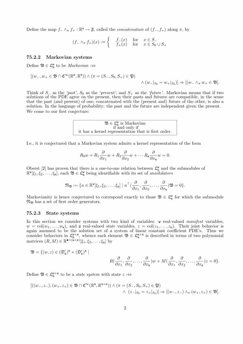
Define the map f− ∧π f+ : Rn → F, called the concatenation of (f−, f+) along π, by

(f− ∧π f+)(x) :=

f−(x) for x ∈ S−f+(x) for x ∈ S0 ∪ S+

75.2.2 Markovian systems

Define B ∈ Lwn to be Markovian :⇔

[(w−, w+ ∈ B ∩ C∞(Rn,Rw)) ∧ (π = (S−, S0, S+) ∈ P)∧ (w−|S0 = w+|S0)]⇒ [(w− ∧π w+ ∈ B].

Think of S− as the ‘past’, S0 as the ‘present’, and S+ as the ‘future’. Markovian means that if twosolutions of the PDE agree on the present, then their pasts and futures are compatible, in the sensethat the past (and present) of one, concatenated with the (present and) future of the other, is also asolution. In the language of probability: the past and the future are independent given the present.We come to our first conjecture:

B ∈ Lwn is Markovian

if and only ifit has a kernel representation that is first order.

I.e., it is conjectured that a Markovian system admits a kernel representation of the form

R0w +R1∂

∂x1w +R2

∂

∂x2w + · · ·Rn

∂

∂xnw = 0.

Oberst [2] has proven that there is a one-to-one relation between Lwn and the submodules of

Rw[ξ1, ξ2, . . . , ξn], each B ∈ Lw

n being identifiable with its set of annihilators

NB := n ∈ Rw[ξ1, ξ2, . . . , ξn] | n>(∂

∂x1,∂

∂x2, . . . ,

∂

∂xn)B = 0.

Markovianity is hence conjectured to correspond exactly to those B ∈ Lwn for which the submodule

NB has a set of first order generators.

75.2.3 State systems

In this section we consider systems with two kind of variables: w real-valued manifest variables,w = col(w1, . . . , ww), and z real-valued state variables, z = col(z1, . . . , zz). Their joint behavior isagain assumed to be the solution set of a system of linear constant coefficient PDE’s. Thus weconsider behaviors in Lw+z

n , whence each element B ∈ Lw+zn is described in terms of two polynomial

matrices (R,M) ∈ R•×(w+z)[ξ1, ξ2, . . . , ξn] by

B = (w, z) ∈ (D′n)w × (D′n)

z |

R(∂

∂x1,∂

∂x2, . . . ,

∂

∂xn)w +M(

∂

∂x1,∂

∂x2, . . . ,

∂

∂xn)z = 0.

Define B ∈ Lw+zn to be a state system with state z :⇔

[((w−, z−), (w+, z+) ∈ B ∩ C∞(Rn,Rw+z)) ∧ (π = (S−, S0, S+) ∈ P)∧ (z−|S0 = z+|S0)]⇒ [(w−, z−) ∧π (w+, z+) ∈ B].

2

Think again of S− as the ‘past’, S0 as the ‘present’, S−+ as the ‘future’. State means that if the statecomponents of two solutions agree on the present, then their pasts and futures are compatible, in thesense that the past of one solution (involving both the manifest and the state variables), concatenatedwith the present and future of the other solution, is also a solution. In the language of probability:the present state ‘splits’ the past and the present plus future of the manifest and the state trajectorycombined.We come to our second conjecture:

B ∈ Lw+zn is a state systemif and only if

it has a kernel representationthat is first order in the state variables z

and zero-th order in the manifest variables w.

I.e., it is conjectured that a state system admits a kernel representation of the form

R0w +M0z +M1∂

∂x1z +M2

∂

∂x2z + · · ·Mn

∂

∂xnz = 0.

75.3 Motivation and history of the problem

These open problems aim at understanding state and state construction for n-D systems.Maxwell’s equations constitute an example of a Markovian system. The diffusion equation and thewave equation are non-examples.

75.4 Available results

It is straightforward to prove the ‘if’-part of both conjectures. The conjectures are true for n = 1,i.e. in the ODE case, see [3].

Bibliography

[1] H.K. Pillai and S. Shankar, A behavioral approach to control of distributed systems, SIAMJournal on Control and Optimization, volume 37, pages 388-408, 1999.

[2] U. Oberst, Multidimensional constant linear systems, Acta Applicandae Mathematicae, volume20, pages 1-175, 1990.

[3] P. Rapisarda and J.C. Willems, State maps for linear systems, SIAM Journal on Control andOptimization, volume 35, pages 1053-1091, 1997.

3

Problem 59

The elusive iff test fortime-controllability of behaviours

Amol SasaneFaculty of Mathematical SciencesUniversity of Twente7500 AE, Enschede,The NetherlandsA.J.Sasane@math.utwente.nl

59.1 Description of the problem

Problem: Let R ∈ C[η1, . . . , ηm, ξ]g×w and let B be the behaviour given by the kernel representationcorresponding to R. Find an algebraic test on R characterizing the time-controllability of B.

In the above, we assume B to comprise of only smooth trajectories, that is,

B =w ∈ C∞

(Rm+1,Cw

)| DRw = 0

,

where DR : C∞(Rm+1,Cw

)→ C∞

(Rm+1,Cg

)is the differential map which acts as follows: if R =[

rij]g×w, then

DR

[ w1...ww

]=

∑w

k=1 r1k

(∂∂x1

, . . . , ∂∂xm

, ∂∂t

)wk

...∑wk=1 rgk

(∂∂x1

, . . . , ∂∂xm

, ∂∂t

)wk

.Time-controllability is a property of the behaviour, defined as follows. The behaviour B is said to betime-controllable if for any w1 and w2 in B, there exists a w ∈ B and a τ ≥ 0 such that

w(•, t) =w1(•, t) for all t ≤ 0w2(•, t− τ) for all t ≥ τ .

59.2 Motivation and history of the problem

The behavioural theory for systems described by a set of linear constant coefficient partial differentialequations has been a challenging and fruitful area of research for quite some time (see for instancePillai and Shankar [5], Oberst [3] and Wood et al. [4]). An excellent elementary introduction to thebehavioural theory in the 1−D case (corresponding to systems described by a set of linear constantcoefficient ordinary differential equations) can be found in Polderman and Willems [6].

4

In [5], [3] and [4], the behaviours arising from systems of partial differential equations are studied ina general setting in which the time-axis does not play a distinguished role in the formulation of thedefinitions pertinent to control theory. Since in the study of systems with “dynamics”, it is useful togive special importance to time in defining system theoretic concepts, recent attempts have been madein this direction (see for example Cotroneo and Sasane [2], Sasane et al. [7] and Camlıbel and Sasane[1]). The formulation of definitions with special emphasis on the time-axis is straightforward, sincethey can be seen quite easily as extensions of the pertinent definitions in the 1−D case. However, thealgebraic characterization of the properties of the behaviour, such as time-controllability, turn out tobe quite involved.Although the traditional treatment of distributed parameter systems (in which one views them as anordinary differential equation with an infinite-dimensional Hilbert space as the state-space) is quitesuccessful, the study of the present problem will have its advantages, since it would give a test whichis algebraic in nature (and hence computationally easy) for a property of the sets of trajectories,namely time-controllability. Another motivation for considering this problem is that the problem ofpatching up of solutions of partial differential equations is also an interesting question from a purelymathematical point of view.

59.3 Available results

In the 1−D case, it is well-known (see for example, Theorem 5.2.5 on page 154 of [6]) that time-controllability is equivalent with the following condition: There exists a r0 ∈ N ∪ 0 such that forall λ ∈ C, rank(R(λ)) = r0. This condition is in turn equivalent with the torsion freeness of theC[ξ]-module C[ξ]w/C[ξ]gR.Let us consider the following statements

A1. The C(η1, . . . , ηm)[ξ]-module C(η1, . . . , ηm)[ξ]w/C(η1, . . . , ηm)[ξ]gR is torsion free.

A2. There exists a χ ∈ C[η1, . . . , ηm, ξ]w\C(η1, . . . , ηm)[ξ]gR and there exists a nonzero p ∈ C[η1, . . . , ηm, ξ]such that p ·χ ∈ C(η1, . . . , ηm)[ξ]gR, and deg(p) = deg((p)), where denotes the homomorphismp(ξ, η1, . . . , ηm) 7→ p(ξ, 0, . . . , 0) : C[ξ, η1, . . . , ηm]→ C[ξ].

In [2], [7] and [1], the following implications were proved:

B is time-controllable⇓ 6⇑ ⇑¬A2 ⇐

6⇒ A1

Although it is tempting to conjecture that the condition A1 might be the iff test for time-controllability,the diffusion equation reveals the precariousness of hazarding such a guess. In [1], it was shown thatthe diffusion equation is time-controllable with respect to1 the space W defined below. Before definingthe set W, we recall the definition of the (small) Gevrey class of order 2, denoted by γ(2)(R): γ(2)(R)is the set of all ϕ ∈ C∞(R,C) such that for every compact set K and every ε > 0 there exists aconstant Cε such that for every k ∈ N, |ϕ(k)(t)| ≤ Cεε

k(k!)2 for all t ∈ K. W is then defined tobe the set of all w ∈ B such that w(0, •) ∈ γ(2)(R). Furthermore, it was also shown in [1], thatthe control could then be implemented by the two point control input functions acting at the pointx = 0: u1(t) = w(0, t) and u2(t) = ∂

∂xw(0, t) for all t ∈ R. The subset W of C∞(R2,C) functionscomprises a large class of solutions of the diffusion equation. In fact, an interesting open problem isthe problem of constructing a trajectory in the behaviour that is not in the class W. Also whether thewhole behaviour (and not just trajectories in W) of the diffusion equation is time-controllable or notis an open question. The answers to these questions would either strengthen or discard the conjecturethat the behaviour corresponding to p ∈ C[η1, . . . , ηm, ξ] is time-controllable iff p ∈ C[η1, . . . , ηm], whichwould eventually help in settling the question of the equivalence of A1 and time-controllability.

1That is, for any two trajectories in W ∩B, there exists a concatenating trajectory in W ∩B.

5

Bibliography

[1] M.K. Camlıbel and A.J. Sasane, “Approximate time-controllability versus time-controllability”.Submitted to the 15th MTNS, U.S.A., June 2002.

[2] T. Cotroneo and A.J. Sasane, “Conditions for time-controllability of behaviours”, InternationalJournal of Control, 75, pp. 61-67 (2002).

[3] U. Oberst, “Multidimensional constant linear systems”, Acta Appl. Math., 20, pp. 1-175 (1990).[4] D.H. Owens, E. Rogers and J. Wood, “Controllable and autonomous n−D linear systems”, Multi-

dimensional Systems and Signal Processing, 10, pp. 33-69 (1999).[5] H.K. Pillai and S. Shankar, “A Behavioural Approach to the Control of Distributed Systems”,

SIAM Journal on Control and Optimization, 37, pp. 388-408 (1998).[6] J.W. Polderman and J.C. Willems, Introduction to Mathematical Systems Theory, Springer-Verlag,

1998.[7] A.J. Sasane, E.G.F. Thomas and J.C. Willems, “Time-autonomy versus time-controllability”. Ac-

cepted for publication in the Systems and Control Letters, 2001.

6

Problem 58

Schur Extremal Problems

Large Lev Sakhnovich

Courant Institute of Mathematical ScienceNew York, NY,11223USALev.Sakhnovich@verizon.net

58.1 Description of the problem

In this paper we consider the well-known Schur problem the solution of which satisfy in addition theextremal condition

w?(z)w(z)≤ρ2min, |z| < 1 (58.1)

where w(z) and ρmin are mxm matrices and ρmin > 0 . Here the matrix ρmin is defined by a certainminimal-rank condition(see Definition 1).We remark that the extremal Schur problem is a particularcase. The general case is considered in book [1] and paper [2].Our approach to the extremal problemsdoesn’t coincide with the superoptimal approach [3],[4].In paper [2] we compare our approach to theextremal problems with the superoptimal approach.Interpolation has found great applications in control theory [5],[6].

Schur extremal problem:The m×m matrices a0, a1, ..., an are given.To describe the set of m×mmatrix functions w(z) holomorphic in the circle |z| < 1 and satisfying the relation

w(z) = a0 + a1z + ...+ anzn + ... (58.2)

and the inequality (1.1)A necessary condition of the solvability of the Schur extremal problem is the inequality

R2min − S≥0 (58.3)

where (n+ 1)m×(n+ 1)m matrices S and Rminare defined by the relations

S = CnC?n, Rmin = diag[ρmin, ρmin, ..., ρmin] (58.4)

Cn =

(a0 0 ... 0a1 a0 ... 0... ... ... ...an an−1 ... a0

)(58.5)

Definition 1.We shall call the matrix ρ = ρmin > 0 a minimal if the the following two requirementsare fulfilled:1. The inequality

R2min − S≥0 (58.6)

is true.2.If m×m matrix ρ > 0 is such that

R2 − S≥0 (58.7)

7

thenrank(R2

min − S)≤rank(R2 − S) (58.8)

where R = diag[ρ, ρ, ..., ρ]Remark 1.The existence of ρmin follows directly from Definition 1.Question 1.Is ρmin unique ?Remark 2.If m=1 then ρmin is unique and ρ2

min = λmax , where λmax is the largest eigenvalue of thematrix S.Remark 3.Under some assumptions the uniqueness of ρmin is proved in the casem > 1,n=1(see [2],[7]).

If ρmin is known then the corresponding wmin(ξ) is a rational matrix function.This generalizes thewell known fact for the scalar case (see[7]).Question 2.How to find ρmin?In order to describe some results in this direction we write the matrix S = CnC

?n in the following block

form (S11 S12S21 S22

)(58.9)

where S22 is the m×m matrix.Proposition 1 [1]If ρ = q > 0 satisfies inequality (1.7) and the relation

q2 = S22 + S?12(Q2 − S11)−1S12 (58.10)

where Q = diag[q, q, ..., q] then ρmin = q.We shall apply the method of successive approximation when studying equation (1.10).We put

q20 = S22, q

2k+1 = S22 + S?12(Q2

k − S11)−1S12 where k≥0, Qk = diag[qk, qk, ..., qk].We suppose that

Q20 − S11 > 0 (58.11)

Theorem 1[1].The sequence q20, q

22, q

24, ... monotonically increases and has the limit m1.The sequence

q21, q

23, q

25, ... monotonically decreases and has the limit m2.The inequality m1≤m2 is true. If m1 = m2

then ρ2min = q2

Question 3.Suppose relation(1.11) holds.Is there a case whenm1 6=m2

The answer is ”no” if n = 1(see[2],[8]).Remark4.In book [1] we give an example in which ρmin is constructed in explicit form.

Bibliography

[1] Lev Sakhnovich”Interpolation Theory and Applications”,it Kluwer Acad.Publ.(1997)[2] J.Helton and L.Sakhnovich ”Extremal Problems of Interpolation Theory”(to appear)[3] N.J.Young”The Nevanlinna-Pick Problem for matrix-valued functions”,it J. Operator Theory,15

pp239-265,(1986).[4] V.V.Peller and N.J.Young ”Superoptimal analytic approximations of matrix functions”,it Journal

of Functional Analysis,120,pp300-343(1994)[5] M.Green M. and D.Limebeer ”Linear Robust Control”it Prentice -Hall(1995)[6] ”Lecture Notes in Control and Information”it Sciences,Springer Verlag, 135,(1989)[7] N.I.Akhiezer ”On a Minimum in Function Theory”,it Operator Theory,Adv. and Appl.95 pp19-

35(1997)[8] A.Ferrante and B.C.Levy ”Hermitian Solutions of the Equations X = Q + NX−1N?”, Linear

Algebra and Applications 247 pp359-373(1996)

8

Problem 69

Regular feedback implementability oflinear differential behaviors

H.L. TrentelmanMathematics Institute,University of GroningenP.O. Box 800,9700 AV GroningenThe Netherlands H.L.Trentelman@math.rug.nl

69.1 Introduction

In this short paper we want to discuss an open problem that appears in the context of interconnectionof systems in a behavioral framework. Given a system behavior, playing the role of plant to becontrolled, the problem is to characterize all system behaviors that can be achieved by interconnectingthe plant behavior with a controller behavior, where the interconnection should be a regular feedbackinterconnection.More specifically, we will deal with linear time-invariant differential systems, i.e., dynamical systemsΣ given as a triple R,Rw,B, where R is the time-axis, and where B, called the behavior of the systemΣ, is equal to the set of all solutions w : R → R

w of a set of higher order, linear, constant coefficient,differential equations. More precisely,

B = w ∈ C∞(R,Rw | R(d

dt)w = 0,

for some polynomial matrix R ∈ R•×w[ξ]. The set of all such systems Σ is denoted by Lw. Often,we simply refer to a system by talking about its behavior, and we write B ∈ Lw instead of Σ ∈ Lw.Behaviors B ∈ Lw can hence be described by differential equations of the form R( ddt)w = 0, typicallywith the number of rows of R strictly less than its number of columns. Mathematically, R( ddt)w = 0 isthen an under-determined system of equations. This results in the fact that some of the componentsof w = (w1, w2, . . . , ww) are unconstrained. This number of unconstrained components is an integer‘invariant’ associated with B, and is called the input cardinality of B, denoted by m(B), its number offree, ‘input’, variables. The remaining number of variables, w − m(B), is called the output cardinalityof B and is denoted by p(B). Finally, a third integer invariant associated with a system behaviorB ∈ Lw is its McMillan degree. It can be shown that (modulo permutation of the componentsof the external variable w) any B ∈ Lw can be represented by a state space representation of theform d

dtx = Ax + Bu, y = Cx + Du, w = (u, y). Here, A,B,C and D are constant matrices withreal components. The minimal number of components of the state variable x needed in such aninput/state/output representation of B is called the McMillan degree of B, and is denoted by n(B).Suppose now Σ1 = R,Rw1 × Rw2 ,B1 ∈ Lw1+w2 and Σ2 = R,Rw2 × Rw3 ,B2 ∈ Lw2+w3 are lineardifferential systems with common factor Rw2 in the signal space. The manifest variable of Σ1 is(w1, w2) and that of Σ2 is (w2, w3). The variable w2 is shared by the systems, and it is through thisvariable, called the interconnection variable, that we can interconnect the systems. We define the

9

interconnection of Σ1 and Σ2 through w2 as the system

Σ1 ∧w2 Σ2 := R,Rw1 × Rw2 × Rw3 ,B1 ∧w2 B2,

with interconnection behavior

B1 ∧w2 B2 := (w1, w2, w3) | (w1, w2) ∈ B1 and (w2, w3) ∈ B2.

The interconnection Σ1 ∧w2 Σ2 is called a regular interconnection if the output cardinalities of Σ1 andΣ2 add up to that of Σ1 ∧w2 Σ2:

p(B1 ∧w2 B2) = p(B1) + p(B2).

It is called a regular feedback interconnection if, in addition, the sum of the McMillan degrees of B1and B2 is equal to the McMilan degree of the interconnection:

n(B1 ∧w2 B2) = n(B1) + n(B2).

It can be proven that the interconnection of Σ1 and Σ2 is a regular feedback interconnection if, possiblyafter permutation of components within w1, w2 and w3, there exists a component-wise partition of w2into w2 = (u, y1, y2), of w1 into w1 = (v1, z1), and of w3 into w3 = (v2, z2) such that the following fourconditions hold:

1. in the system Σ1, (v1, y2, u) is input and (z1, y1) is output, and the transfer matrix from (v1, y2, u)to (z1, y1) is proper

2. in the system Σ2, (v2, y1, u) is input and (z2, y2) is output, and the transfer matrix from (v2, y1, u)to (z2, y2) is proper

3. in the system Σ1 ∧w2 Σ2, (v1, v2, u) is input and (z1, z2, y1, y2) is output, and the transfer matrixfrom (v1, v2, u) to (z1, z2, y1, y2) is proper.

4. if we introduce new (‘perturbation signals’) e1 and e2 and, instead of y1 and y2 we apply inputsy1 + e2 and y2 + e1 to Σ2 and Σ1 respectively, then the transfer matrix from (v1, v2, u, e1, e2) to(z1, z2, y1, y2) is proper.

The first three of these conditions state that, in the interconnection of Σ1 and Σ2, along the terminalsof the interconnected system one can identify a signal flow which is compatible with the signal flowdiagram of a feedback configuration with proper transfer matrices. The fourth condition states thatthis feedback interconnection is ‘well-posed’ . The equivalence of the property of being a regularfeedback interconnection with these four conditions was studied for the ‘full interconnection case’ in[8] and [2].

69.2 Statement of the problem

Suppose Pfull ∈ Lw+c is a system (the plant) with two types of external variables, namely c and w.The first of these, c, is the interconnection variable through which it can be interconnected to a secondsystem C ∈ Lc (the controller) with external variable c. The external variable c is shared by Pfulland C. The remaining variable w is the variable through which Pfull interacts with the rest of itsenvironment. After interconnecting plant and controller through the shared variable c, we obtain thefull controlled behavior Pfull ∧c C ∈ Lw+c. The manifest controlled behavior K ∈ Lw is obtained byprojecting all trajectories (w, c) ∈ Pfull ∧c C on their first coordinate:

K := w | there exists c such that (w, c) ∈ Pfull ∧c C. (69.1)

If this holds, then we say that C implements K. If, for a given K ∈ Lw there exists C ∈ Lc such thatC implements K, then we call K implementable. If, in addition, the interconnection of Pfull and C isregular, we call K regularly implementable. Finally, if the interconnection of Pfull and C is a regularfeedback interconnection, we call K implementable by regular feedback.

10

This now brings us to the statement of our problem: the problem is to characterize, for a givenPfull ∈ Lw+c, the set of all behaviors K ∈ Lw that are implementable by regular feedback. In otherwords:

Problem statement: Let Pfull ∈ Lw+c be given. Let K ∈ Lw. Find necessary andsufficient conditions on K under which there exists C ∈ Lc such that

1. C implements K (meaning that (69.1) holds),

2. p(Pfull ∧c C) = p(Pfull) + p(C),

3. n(Pfull ∧c C) = n(Pfull) + n(C).

Effectively, a characterization of all such behaviors K ∈ Lw gives a characterization of the ‘limits ofperformance’ of the given plant under regular feedback control.

69.3 Background

Our open problem is to find conditions for a given K ∈ Lw to be implementable by regular feedback.An obvious necessary condition for this is that K is implementable, i.e., it can be achieved by in-terconnecting the plant with a controller by (just any) interconnection through the interconnectionvariable c. Necessary and sufficient conditions for implementability have been obtained in [7]. Theseconditions are formulated in terms of two behaviors derived from the full plant behavior Pfull:

P := w | there exists c such that (w, c) ∈ Pfull

andN := w | (w, 0) ∈ Pfull.

P and N are both in Lw, and are called the manifest plant behavior and hidden behavior associatedwith the full plant behavior Pfull, respectively. In [7] it has been shown that K ∈ Lw is implementableif and only if

N ⊆ K ⊆ P, (69.2)

i.e., K contains N, and is contained in P. This elegant characterization of the set of implementablebehaviors still holds true if, instead of (ordinary) linear differential system behaviors, we deal withnD linear system behaviors, which are system behaviors that can be represented by partial differentialequations of the form

R(∂

∂x1,∂

∂x2, . . . ,

∂

∂xn)w(x1, x2, . . . , xn) = 0,

with R(ξ1, ξ2, . . . , ξn) a polynomial matrix in n indeterminates. Recently, in [6] a variation of condition(69.2) was shown to be sufficient for implementability of system behaviors in a more general (includingnon-linear) context.For a system behavior K ∈ Lw to be implementable by regular feedback, another necessary conditionis of course that K is regularly implementable, i.e., it can be achieved by interconnecting the plantwith a controller by regular interconnection through the interconnection variable c. Also for regularimplementability necessary and sufficient conditions can already be found in the literature. In [1], ithas been shown that a given K ∈ Lw is regularly implementable if and only if, in addition to condition(69.2), the following condition holds:

K + Pcont = P. (69.3)

Condition (69.3) states that the sum of K and the controllable part of P is equal to P. The controllablepart Pcont of the behavior P is defined as the largest controllable subbehavior of P, which is the uniquebehavior Pcont with the properties that 1.) Pcont ⊆ P, and 2.) P′ controllable and P′ ⊆ P impliesP′ ⊆ Pcont. Clearly, if the manifest plant behavior P is controllable, then P = Pcont, so condition(69.3) automatically holds. In this case, implementability and regular implementability are equivalent

11

properties. For the special case N = 0 (which is equivalent to the ’full interconnection case’), conditions(69.2) and (69.3) for regular implementability in the context of nD system behaviors can also be foundin [19]. In the same context, results on regular implementability can also be found in [9].We finally note that, again for the full interconnection case, the open problem stated in this paper hasrecently been studied in [3], using a somewhat different notion of linear system behavior, in discretetime. Up to now, however, the general problem has remained unsolved.

Bibliography

[1] M.N. Belur and H.L. Trentelman, Stabilization, pole placement and regular implementability, toappear in IEEE Transactions on Automatic Control, May 2002.

[2] M. Kuijper, Why do stabilizing controllers stabilize, Automatica, volume 31, pages 621-625, 1995.[3] V. Lomadze, On interconnections and control, manuscript, 2001.[4] P. Rocha and J. Wood, Trajectory control and interconnection of nD systems, SIAM Journal on

Contr. and Opt., Vol. 40, Number 1, pages 107-134, 2001.[5] J.W. Polderman and J.C. Willems, Introduction to Mathematical Systems Theory: A Behavioral

Approach, Springer Verlag, 1997.[6] A.J. van der Schaft, Achievable behavior of general systems, manuscript 2002, submitted for

publication.[7] J.C. Willems and H.L. Trentelman, Synthesis of dissipative systems using quadratic differential

forms, Part 1, IEEE Transactions on Automatic Control, Vol. 47, No. 1, pages 53-69, 2002.[8] J.C. Willems, On Interconnections, Control and Feedback, IEEE Transactions on Automatic

Control, volume 42, pages 326-337, 1997.[9] E. Zerz and V. Lomadze, A constructive solution to interconnection and decomposition problems

with multidimensional behaviors, SIAM Journal on Contr. and Opt., Vol. 40, Number 4, pages1072-1086, 2001.

12

Problem 36

What is the characteristic polynomialof a signal flow graph?

Andrew D. LewisDepartment of Mathematics & StatisticsQueen’s UniversityKingston, ON K7L 3N6Canadaandrew@mast.queensu.ca

36.1 Problem statement

Suppose one is given signal flow graph G with n nodes whose branches have gains that are real rationalfunctions (the open loop transfer functions). The gain of the branch connecting node i to node j isdenoted Rji, and we write Rji = Nji

Djias a coprime fraction. The closed-loop transfer function from

node i to node j for the closed-loop system is denoted Tji.The problem can then be stated as follows.

Is there an algorithmic procedure that takes a signal flow graph G and returns a “characteristic poly-nomial” PG with the following properties:

1. the construction of PG depends only on the topology of the graph, and not on manipulations ofthe branch gains;

2. all closed-loop transfer functions Tji, i, j = 1, . . . , n, are analytic in the closed right half plane(CRHP) if and only if PG is Hurwitz?

The condition 1 is a little vague. It may be thought of as a sort of “meta-condition,” and perhaps canbe replaced with something like

1’. PG is formed by products and sums of the polynomials Nji and Dji, i, j = 1, . . . , n.

The idea is that the definition of PG should not depend on the choice of branch gains Rji, i, j = 1, . . . , n.For example, one would be prohibited from factoring polynomials or from computing the GCD ofpolynomials. This excludes unhelpful solutions of the problem of the form “Let PG be the product ofthe characteristic polynomials of the closed-loop transfer functions Tji, i, j = 1, . . . , n.”

36.2 Discussion

Signal flow graphs for modelling system interconnections are due to Mason [3, 4]. Of course, whenmaking such interconnections, the stability of the interconnection is nontrivially related to the open-loop transfer functions that weight the branches of the signal flow graph. There are two things to

13

consider in the course of making an interconnection: (1) is the interconnection internally stable in thesense that all closed-loop transfer functions between nodes have no poles in the CRHP? and (2) isthe interconnection well-posed in the sense that all closed-loop transfer functions between nodes areproper? The problem stated above concerns only the first of these matters. Well-posedness whenall branch gains Rji, i, j = 1, . . . , n, are proper is known to be equivalent to the condition that thedeterminant of the graph be a biproper rational function.As an illustration of what we are after, consider the single-loop configuration of Figure 36.1. As is

-r d -R1(s) -R2(s) - y6−

Figure 36.1: Single-loop interconnection

well-known, if we write Ri = NiDi

, i = 1, 2, as coprime fractions, then all closed-loop transfer functionshave no poles in the CRHP if and only if the polynomial PG = D1D2 + N1N2 is Hurwitz. Thus PGserves as the characteristic polynomial in this case. The essential feature of PG is that one computes itby looking at the topology of the graph, and the exact character of R1 and R2 are of no consequence.For example, pole/zero cancellations between R1 and R2 are accounted for in PG.

36.3 Approaches that do not solve the problem

Let us outline two approaches that yield solutions having one of properties 1 and 2, but not the other.The problems of internal stability and well-posedness for signal flow graphs can be handled effectivelyusing the polynomial matrix approach e.g., [1]. Such an approach will involve the determinationof a coprime matrix fractional representation of a matrix of rational functions. This will certainlysolve the problem of determining internal stability for any given example. That is, it is possibleusing matrix polynomial methods to provide an algorithmic construction of a polynomial satisfyingproperty 2 above. However, the algorithmic procedure will involve computing GCD’s of various of thepolynomials Nji and Dji, i, j = 1, . . . , n. Thus the conditions developed in this manner have to do notonly with the topology of the signal flow graph, but also the specific choices for the branch gains, thusviolating condition 1 (and 1’) above. The problem we pose demands a simpler, more direct answer tothe question of determining when an interconnection is internally stable.Wang, Lee, and He [5] propose a characteristic polynomial for a signal flow graph using the determinantof the graph which we denote by ∆G (see [3, 4]). Specifically, they suggest using

P =∏

(i,j)∈1,...,n2Dji∆G (36.1)

as the characteristic polynomial. Thus one multiplies the determinant by all denominators, arrivingat a polynomial in the process. This polynomial has the property 1 (or 1’) above. However, while it istrue that if this polynomial is Hurwitz then the system is internally stable, the converse is false (see [2]for a simple counterexample). Thus property 2 is not satisfied by P . It is true that the polynomial Pin (36.1) gives the correct characteristic polynomial for the interconnection of Figure 36.1. It is alsotrue that if the signal flow graph has no loops (in this case ∆G = 1) then the polynomial P of (36.1)satisfies condition 2.The problem stated is very basic, one for which an inquisitive undergraduate would demand a solution.It was with some surprise that the author was unable to find its solution in the literature, and hopefullyone of the readers of this article will be able to provide a solution, or point out an existing one.

Bibliography

[1] F. M. Callier and C. A. Desoer. Multivariable Feedback Systems. Springer-Verlag, New York-Heidelberg-Berlin, 1982.

14

[2] A. D. Lewis. On the stability of interconnections of SISO, time-invariant, finite-dimensional, linearsystems. Preprint, July 2001.

[3] S. J. Mason. Feedback theory: Some properties of signal flow graphs. Proc. IRE, 41:1144–1156,1953.

[4] S. J. Mason. Feedback theory: Further properties of signal flow graphs. Proc. IRE, 44:920–926,1956.

[5] Q.-G. Wang, T.-H. Lee, and J.-B. He. Internal stability of interconnected systems. IEEE Trans.Automat. Control, 44(3):593–596, 1999.

15

Problem 35

Bases for Lie algebras and a continuousCBH formula

Matthias Kawski1

Department of Mathematics and StatisticsArizona State University,Tempe, Arizona 85287-1804USAkawski@asu.edu

35.1 Description of the problem

Many time-varying linear systems x = F (t, x) naturally split into time-invariant geometric componentsand time-dependent parameters. A special case are nonlinear control systems that are affine in thecontrol u, and specified by analytic vector fields on a manifold Mn

x = f0(x) +m∑k=1

uk fk(x). (35.1)

It is natural to search for solution formulas for x(t) = x(t, u) that, separate the time-dependentcontributions of the controls u from the invariant, geometric role of the vector fields fk. Ideally,one may be able to a-priori obtain closed-form expressions for the flows of certain vector fields. Thequadratures of the control might be done in real-time, or the integrals of the controls may be considerednew variables for theoretical purposes such as path-planning or tracking.To make this scheme work, one needs simple formulas for assembling these pieces to obtain the solutioncurve x(t, u). Such formulas are nontrivial since in general the vector fields fk do not commute: alreadyin the case of linear systems, exp(sA) · exp(tB) 6= exp(sA + tB) (for matrices A and B). Thus thedesired formulas not only involve the flows of the system vector fields fi, but also the flows of theiriterated commutators [fi, fj ], [[fi, fj ], fk], and so on.Using Hall-Viennot bases H for the free Lie algebra generated by m indeterminates X1, . . . Xm, Suss-mann [16] gave a general formula as a directed infinite product of exponentials

x(T, u) =→∏

H∈H

exp(ξH(T, u) · fH). (35.2)

Here the vector field fH is the image of the formal bracket H under the canonical Lie algebra ho-momorphism that maps Xi to fi. Using the chronological product (U ∗ V )(t) =

∫ T0 U(s)V ′(s) ds, the

iterated integrals ξH are defined recursively by ξXk(T, u) =∫ T

0 uk(t)dt and

ξHK = ξH ∗ ξK (35.3)1Supported in part by NSF-grant DMS 00-72369

16

if H,K,HK are Hall words and the left factor of K is not equal to H [9, 16]. (In the case of repeatedleft factors, the formula contains an additional factorial.)

An alternative to such infinite exponential product (in Lie group language: “coordinates of the 2nd

kind”) is a single exponential of an infinite Lie series (“coordinates of the 1st kind”).

x(T, u) = exp(∑B∈B

ζB(T, u) · fB) (35.4)

It is straightforward to obtain explicit formulas for ζB for some spanning sets B of the free Lie algebra[16], but much preferable are series that use bases B, and which, in addition, yield as simple formulasfor ζB as (35.3) does for ξH .

Problem 1. Construct bases B = Bk : k ≥ 0 for the free Lie algebra on a finite number of generatorsX1, . . . Xm such that the corresponding iterated integral functionals ζB defined by (35.4) have simpleformulas (similar to (35.3)), suitable for control applications (both analysis and design).

The formulae (35.4) and (35.2) arise from the “free control system” on the free associative algebraon m generators. Its universality means that its solutions map to solutions of specific systems (27.1)on Mn via the evaluation homomorphism Xi 7→ fi. However, the resulting formulas contain manyredundant terms since the vector fields fB are not linearly independent.

Problem 2. Provide an algorithm that generates for any finite collection of analytic vector fieldsF = f1, . . . , fm on Mn a basis for L(f1, . . . , fm) together with effective formulas for associatediterated integral functionals.

Without loss of generality one may assume that the collection F satisfies the Lie algebra rank condition.i.e. L(f1, . . . , fm)(p) = TpM at a specified initial point p. It makes sense to first consider specialclasses of systems F, e.g. which are such that L(f1, . . . , fm) is finite, nilpotent, solvable, etc. Thewords simple and effective are not used in a technical sense in problems 1 and 2 (as in formal studiesof computational complexity), but instead refer to comparison with the elegant formula (35.3), whichhas proven convenient for theoretical studies, numerical computation, and practical implementations.

35.2 Motivation and history of the problem

Series expansions of solution to differential equations have a long history. Elementary Picard iterationof the universal control system S =

∑mi=1Xiui on the free associative algebra over X1, . . . , Xm yields

the Chen Fliess series [2, 11, 21]. Other major tools are Volterra series, and the Magnus expansion [14],which groups the terms in a different way than the Fliess series. The main drawback of the Fliessseries is that (unlike its exponential product expansion (35.2)) no finite truncation is the exact solutionof any approximating system. A key innovation is the chronological calculus of 1970s Agrachev andGamkrelidze [1]. However, it is generally not formulated using explicit bases.The series and product expansions have manifold uses in control beyond simple computation of integralcurves, and analysis of reachable sets (which includes controllability and optimality). These includestate-space realizations of systems given in input-output operator form [8, 20], output tracking andpath-planning. For the latter, express the target or reference trajectory in terms of the ξ or ζ, nowconsidered as coordinates of a suitably lifted system (e.g. free nilpotent) and invert the restrictionof the map u 7→ ξB : B ∈ BN or u 7→ ζB : B ∈ BN (for some finite subbasis BN ) to a finitelyparameterized family of controls u, e.g. piecewise polynomial [7] or trigonometric polynomial [10, 17].The Campbell-Baker-Hausdorff formula [18] is a classic tool to combine products of exponentials intoa single exponential eaeb = eH(a,b) where H(a, b) = a + b + 1

2 [a, b] + 112 [a, [a, b]] − 1

12 [b, [a, b] + . . .. Ithas been extensively used for designing piecewise constant control variations that generate high ordertangent vectors to reachable sets, e.g. for deriving conditions for optimality. However, repeated useof the formula quickly leads to unwieldily expressions. The expansion (35.2) is the natural continuousanalogue of the CBH formula – and the problem is to find the most useful form.The uses of these expansions (35.2) and (35.4) extend far beyond control, as they apply to any dynam-ical systems that split into different interacting components. In particular, closely related techniques

17

have recently found much attention in numerical analysis. This started with a search for Runge-Kutta-like integration schemes such that the approximate solutions inherently satisfy algebraic constraints(e.g. conservation laws) imposed on the dynamical system [3]. Much effort has been devoted to op-timize such schemes, in particular minimizing the number of costly function evaluations [16]. For arecent survey see [6]. Clearly the form (35.4) is most attractive as it requires the evaluation of only asingle (computationally costly) exponential.The general area of noncommuting formal power series admits both dynamical systems / analyticand purely algebraic / combinatorial approaches. Algebraically, underlying the expansions (35.2)and (35.4) is the Chen series [2], which is well known to be an exponential Lie series, compare [18],thus guaranteeing the existence of the alternative expansions

∑w∈Z∗

w ⊗ w != exp( ∑

B∈B

ζB ⊗B)

!=→∏B∈B

exp (ξB ⊗B) (35.5)

The first bases for free Lie algebras build on Hall’s work in the 1930s on commutator groups. Whileseveral other bases (Lyndon, Sirsov) have been proposed in the sequel, Viennot [23] showed that theyare all special cases of generalized Hall bases. Underlying their construction is a unique factorizationprinciple, which in turn is closely related to Poincare-Birckhoff-Witt bases (of the universal envelopingalgebra of a Lie algebra) and Lazard elimination. Formulas for the dual PBW bases ξB have been givenby Schutzenberger, Sussmann[16], Grossman, and Melancon and Reutenauer [15]. For an introductorysurvey see [11], while [15] elucidates the underlying Hopf algebra structure, and [18] is the principaltechnical reference for combinatorics of free Lie algebras.

35.3 Available related results

The direct expansion of the logarithm into a formal power series may be simplified using symmetriza-tion [18, 16], but this still does not yield well-defined “coordinates” with respect to a basis.Explicit, but quite unattractive formulas forthe first 14 coefficients ζH in the case of m = 2 and a Hallbasis are calculated in [10]. This calculation can be automated in a computer algebra system for termsof considerably higher order, but no apparent algebraic structure is discernible. These results sufficefor some numerical purposes, but they don’t provide much structural insight.Several new algebraic structures introduced in [19] lead to systematic formulas for ζB using spanningsets B that are smaller than those in [16], but are not bases. These formulas can be refined to apply toHall-bases, but at the cost of loosing their simple structure. Further recent insights into the underlyingalgebraic structures may be found in [4, 13].The introductory survey [11] lays out in elementary terms the close connections between Lazardelimination, Hall-sets, chronological products, and the particularly attractive formula (35.3). Theseintimate connections suggest that to obtain similarly attractive expressions for ζB one may have tostart from the very beginning by building bases for free Lie algebras that do not rely on recursiveuse of Lazard elimination. While it is desirable that any such new bases still restrict to bases ofthe homogeneous subspaces of the free Lie algebra, we suggest consider balancing the simplicity ofthe basis for the Lie algebra and structural simplicity of the formulas for the dual objects ζB. Inparticular, consider bases whose elements are not necessarily Lie monomials, but possibly nontriviallinear combinations of iterated Lie brackets of the generators.

Bibliography

[1] A. Agrachev and R. Gamkrelidze, “Chronological algebras and nonstationary vector fields”, Jour-nal Soviet Math., 17, pp. 1650–1675 (1979).

[2] K. T. Chen, “Integration of paths, geometric invariants and a generalized Baker-Hausdorff for-mula”, Annals of Mathematics, 65, pp. 163–178 (1957).

[3] P. Crouch and R. Grossman, “The explicit computation of integration algorithms and first integralsfor ordinary differential equations with polynomial coefficients using trees”, Proc. Int. Symposiumon Symbolic and Algebraic Computation, pp. 89-94, ACM Press (1992).

18

[4] A. Dzhumadil’daev, “Non-associative algebras without unit”, Comm. Algebra (2002) (to appear).[5] M. Fliess, “Fonctionelles causales nonlineaires et indeterminees noncommutatives”, Bull. Soc.

Math. France, 109, pp. 3–40 (1981).[6] A. Iserles, “Expansions that grow on trees”, Notices AMS, 49, pp. 430-440 (2002).[7] G. Jacob, “Motion planning by piecewise constant or polynomial inputs”, Proc. NOLCOS, Bor-

deaux (1992).[8] B. Jakubczyk, “Convergence of power series along vector fields and their commutators; a Cartan-

Kahler type theorem,” Ann. Polon. Math., 74, pp. 117-132, (2000).[9] M. Kawski and H. J. Sussmann “Noncommutative power series and formal Lie-algebraic techniques

in nonlinear control theory”, in: Operators, Systems, and Linear Algebra, U. Helmke, D. Pratzel-Wolters and E. Zerz, eds., pp. 111–128, Teubner (1997).

[10] M. Kawski, “Calculating the logarithm of the Chen Fliess series”, Proc. MTNS, Perpignan (2000).[11] M. Kawski, “The combinatorics of nonlinear controllability and noncommuting flows”, Lecture

Notes series of the Abdus Salam ICTP (2001).[12] G. Lafferriere and H. Sussmann, “Motion planning for controllable systems without drift”, Proc.

Int. Conf. Robot. Automat., pp. 1148–1153 (1991).[13] J.-L. Loday and T. Pirashvili, “Universal enveloping algebras of Leibniz algebras and

(co)homology”, Math. Annalen, 196, pp. 139–158 (1993).[14] W. Magnus, “On the exponential solution of differential equations for a linear operator” Comm.

Pure Appl. Math., VII, pp. 649–673 (1954).[15] G. Melancon and C. Reutenauer, “Lyndon words, free algebras and shuffles”, Canadian J. Math.,

XLI, pp. 577–591 (1989).[16] H. Munthe-Kaas and B. Owren, “Computations in a free Lie algebra”, Royal Soc.London Phi-

los.Trans.Ser.A Math.Phys.Eng.Sci., 357, pp. 957–982 (1999).[17] R. Murray and S. Sastry, “Nonholonomic path planning: steering with sinusoids”, IEEE

Trans.Aut.Control, 38, pp. 700–716 (1993).[18] C. Reutenauer, “Free Lie algebras”, (1993), Oxford (Clarendon Press).[19] E. Rocha, “On computataion of the logarithm of the Chen-Fliess series for nonlinear systems”,

Proc. NCN, Sheffield (2001).[20] E. Sontag and Y. Wang, ““Orders of input/output differential equations and state space dimen-

sions,” SIAM J. Control and Optimization, 33, pp. 1102-1126 (1995).[21] H. Sussmann, “Lie brackets and local controllability: a sufficient condition for scalar-input sys-

tems”, SIAM J. Cntrl. & Opt., 21, pp. 686–713 (1983).[22] H. Sussmann, “A product expansion of the Chen series”, Theory and Applications of Nonlinear

Control Systems, C. I. Byrnes and A. Lindquist eds., Elsevier, North-Holland (1986), 323–335.[23] G. Viennot, “Algebres de Lie Libres et Monoides Libres”, Lecture Notes Math., 692, Springer,

Berlin, (1978).

19

Problem 10

Vector-valued quadratic forms incontrol theory

Francesco BulloCoordinated Science LaboratoryUniversity of IllinoisUrbana-Champaign, IL 61801USAbullo@uiuc.edu

Jorge CortesSystems, Signals and ControlUniversity of TwenteEnschede, 7500 AEThe Netherlandsj.cortesmonforte@utwente.nl

Andrew D. LewisMathematics & StatisticsQueen’s UniversityKingston, ON K7L 3N6Canadaandrew@mast.queensu.ca

Sonia MartınezInstitute of Mathematics & PhysicsHigh Council of Scientific ResearchMadrid, 28006Spains.martinez@imaff.cfmac.csic.es

10.1 Problem statement and historical remarks

For finite dimensional R-vector spaces U and V we consider a symmetric bilinear map B : U ×U → V .This then defines a quadratic map QB : U → V by QB(u) = B(u, u). Corresponding to each λ ∈ V ∗is a R-valued quadratic form λQB on U defined by λQB(u) = λ ·QB(u). B is definite if there existsλ ∈ V ∗ so that λQB is positive-definite. B is indefinite if for each λ ∈ V ∗ \ ann(image(QB)), λQB isneither positive nor negative-semidefinite, where ann denotes the annihilator.

Given a symmetric bilinear map B : U × U → V , the problems we consider are as follows.

1. Find necessary and sufficient conditions characterizing when QB is surjective.

2. If QB is surjective and v ∈ V , design an algorithm to find a point u ∈ Q−1B (v).

20

3. Find necessary and sufficient conditions to determine when B is indefinite.

¿From the computational point of view, the first two questions are the more interesting ones. Bothcan be shown to be NP-complete, whereas the third one can be recast as a semidefinite programmingproblem.1 Actually, our main interest is in a geometric characterization of these problems. Section 10.4below constitutes an initial attempt to unveil the essential geometry behind these questions. Byunderstanding the geometry of the problem properly, one may be lead to simple characterizations likethe one presented in Proposition 3, which turn out to be checkable in polynomial time for certainclases of quadratic mappings.Before we comment on how our problem impinges on control theory, let us provide some historicalcontext for it as a purely mathematical one. The classification of R-valued quadratic forms is wellunderstood. However, for quadratic maps taking values in vector spaces of dimension two or higher, theclassification problem becomes more difficult. The theory can be thought of as beginning with the workof Kronecker, who obtained a finite classification for pairs of symmetric matrices. For three or moresymmetric matrices, that the classification problem has an uncountable number of equivalence classesfor a given dimension of the domain follows from the work of Kac [12]. For quadratic forms, in a seriesof papers Dines (see [8] and references cited therein) investigated conditions when a finite collection ofR-valued quadratic maps were simultaneously positive-definite. The study of vector-valued quadraticmaps is ongoing. A recent paper is [13], to which we refer for other references.

10.2 Control theoretic motivation

Interestingly and perhaps not obviously, vector-valued quadratic forms come up in a variety of placesin control theory. We list a few of these here.

Optimal control: Agrachev [2] explicitly realises second-order conditions for optimality in termsof vector-valued quadratic maps. The geometric approach leads naturally to the consideration ofvector-valued quadratic maps, and here the necessary conditions involve definiteness of these maps.Agrachev and Gamkrelidze [1, 3] look at the map λ 7→ λQB from V ∗ into the set of vector-valuedquadratic maps. Since λQB is a R-valued quadratic form, one can talk about its index and rank (thenumber of −1’s and nonzero terms, respectively, along the diagonal when the form is diagonalised).In [1, 3] the topology of the surfaces of constant index of the map λ 7→ λQB is investigated.

Local controllability: The use of vector-valued quadratic forms arises from the attempt to arriveat feedback-invariant conditions for controllability. Basto-Goncalves [6] gives a second-order sufficientcondition for local controllability, one of whose hypotheses is that a certain vector-valued quadraticmap be indefinite (although the condition is not stated in this way). This condition is somewhat refinedin [11], and a necessary condition for local controllability is also given. Included in the hypotheses ofthe latter is the condition that a certain vector-valued quadratic map be definite.

Control design via power series methods and singular inversion: Numerous control designproblems can be tackled using power series and inversion methods. The early references [5, 9] show howto solve the optimal regulator problem and the recent work in [7] proposes local steering algorithms.These strong results apply to linearly controllable systems, and no general methods are yet availableunder only second-order sufficient controllability conditions. While for linearly controllable systemsthe classic inverse function theorem suffices, the key requirement for second-order controllable systemsis the ability to check surjectivity and compute an inverse function for certain vector-valued quadraticforms.

Dynamic feedback linearisation: In [14] Sluis gives a necessary condition for the dynamic feed-back linearisation of a system

x = f(x, u), x ∈ Rn, u ∈ Rm.The condition is that for each x ∈ Rn, the set Dx = f(x, u) ∈ TxRn| u ∈ Rm admits a ruling , thatis, a foliation of Dx by lines. Some manipulations with differential forms turns this necessary condition

1We thank an anonymous referee for these observations.

21

into one involving a symmetric bilinear map B. The condition, it turns out, is that Q−1B (0) 6= 0.

This is shown by Agrachev [1] to generically imply that QB is surjective.

10.3 Known results

Let us state a few results along the lines of our problem statement that are known to the authors.The first is readily shown to be true (see [11] for the proof). If X is a topological space with subsetsA ⊂ S ⊂ X, we denote by intS(A) the interior of A relative to the induced topology on S. If S ⊂ V ,aff(S) and conv(S) denote, respectively, the affine hull and the convex hull of S.

Proposition 1 Let B : U × U → V be a symmetric bilinear map with U and V finite-dimensional.The following statements hold:

(i) B is indefinite if and only if 0 ∈ intaff(image(QB))(conv(image(QB)));

(ii) B is definite if and only if there exists a hyperplane P ⊂ V so that image(QB) ∩ P = 0 andso that image(QB) lies on one side of P ;

(iii) if QB is surjective then B is indefinite.

The converse of (iii) is false. The quadratic map from R3 to R3 defined by QB(x, y, z) = (xy, xz, yz)

may be shown to be indefinite but not surjective.Agrachev and Sarychev [4] prove the following result. We denote by ind(Q) the index of a quadraticmap Q : U → R on a vector space U .

Proposition 2 Let B : U × U → V be a symmetric bilinear map with V finite-dimensional. Ifind(λQB) ≥ dim(V ) for any λ ∈ V ∗ \ 0 then QB is surjective.

This sufficient condition for surjectivity is not necessary. The quadratic map from R2 to R2 given by

QB(x, y) = (x2 − y2, xy) is surjective, but does not satisfy the hypotheses of Proposition 2.

10.4 Problem simplification

One of the difficulties with studying vector-valued quadratic maps is that they are somewhat difficultto get ones hands on. However, it turns out to be possible to simplify their study by a reduction to arather concrete problem. Here we describe this process, only sketching the details of how to go froma given symmetric bilinear map B : U × U → V to the reformulated end problem. We first simplifythe problem by imposing an inner product on U and choosing an orthonormal basis so that we maytake U = R

n.We let Symn(R) denote the set of symmetric n × n matrices with entries in R. On Symn(R) we usethe canonical inner product

〈A,B〉 = tr(AB).

We consider the map π : Rn → Symn(R) defined by π(x) = xxt, where t denotes transpose. Thus theimage of π is the set of symmetric matrices of rank at most one. If we identify Symn(R) ' Rn ⊗ Rn,then π(x) = x⊗ x. Let Kn be the image of π and note that it is a cone of dimension n in Symn(R)having a singularity only at its vertex at the origin. Furthermore, Kn may be shown to be a subset ofthe hypercone in Symn(R) defined by those matrices A in Symn(R) forming angle arccos( 1

n) with theidentity matrix. Thus the ray from the origin in Symn(R) through the identity matrix is an axis forthe cone KN . In algebraic geometry, the image of Kn under the projectivisation of Symn(R) is knownas the Veronese surface [10], and as such is well-studied, although perhaps not along lines that beardirectly on the problems of interest in this article.We now let B : Rn × Rn → V be a symmetric bilinear map with V finite-dimensional. Using theuniversal mapping property of the tensor product, B induces a linear map B : Symn(R) ' Rn⊗Rn → V

with the property that B π = B. The dual of this map gives an injective linear map B∗ : V ∗ →

22

Symn(R) (here we assume that the image of B spans V ). By an appropriate choice of inner product onV one can render the embedding B∗ an isometric embedding of V in Symn(R). Let us denote by LBthe image of V under this isometric embedding. One may then show that with these identifications,the image of QB in V is the orthogonal projection of Kn onto the subspace LB. Thus we reduce theproblem to one of orthogonal projection of a canonical object, Kn, onto a subspace in Symn(R)! Tosimplify things further, we decompose LB into a component along the identity matrix in Symn(R)and a component orthogonal to the identity matrix. However, the matrices orthogonal to the identityare readily seen to simply be the traceless n × n symmetric matrices. Using our picture of Kn as asubset of a hypercone having as an axis the ray through the identity matrix, we see that questionsof surjectivity, indefiniteness, and definiteness of B impact only on the projection of Kn onto thatcomponent of LB orthogonal to the identity matrix.The following summarises the above discussion.

The problem of studying the image of a vector-valued quadratic form can be reduced to studying theorthogonal projection of Kn ⊂ Symn(R), the unprojectivised Veronese surface, onto a subspace of thespace of traceless symmetric matrices.

This is, we think, a beautiful interpretation of the study of vector-valued quadratic mappings, andwill surely be a useful formulation of the problem. For example, with it one easily proves the followingresult.

Proposition 3 If dim(U) = dim(V ) = 2 with B : U ×U → V a symmetric bilinear map, then QB issurjective if and only if B is indefinite.

Bibliography

[1] A. A. Agrachev. The topology of quadratic mappings and Hessians of smooth mappings. J. SovietMath., 49(3):990–1013, 1990.

[2] A. A. Agrachev. Quadratic mappings in geometric control theory. J. Soviet Math., 51(6):2667–2734, 1990.

[3] A. A. Agrachev and R. V. Gamkrelidze. Quadratic mappings and vector functions: Euler char-acteristics of level sets. J. Soviet Math., 55(4):1892–1928, 1991.

[4] A. A. Agrachev and A. V. Sarychev. Abnormal sub-Riemannian geodesics: Morse index andrigidity. Ann. Inst. H. Poincare. Anal. Non Lineaire, 13(6):635–690, 1996.

[5] E. G. Al’brekht. On the optimal stabilization of nonlinear systems. J. Appl. Math. and Mech.,25:1254–1266, 1961.

[6] J. Basto-Goncalves. Second-order conditions for local controllability. Systems Control Lett.,35(5):287–290, 1998.

[7] W. T. Cerven and F. Bullo. Constructive controllability algorithms for motion planning andoptimization. Preprint, November 2001.

[8] L. L. Dines. On linear combinations of quadratic forms. Bull. Amer. Math. Soc. (N.S.), 49:388–393, 1943.

[9] A. Halme. On the nonlinear regulator problem. J. Optim. Theory Appl., 16(3-4):255–275, 1975.[10] J. Harris. Algebraic Geometry: A First Course. Number 133 in Graduate Texts in Mathematics.

Springer-Verlag, New York-Heidelberg-Berlin, 1992.[11] R. M. Hirschorn and A. D. Lewis. Geometric local controllability: Second-order conditions.

Preprint, February 2002.[12] V. G. Kac. Root systems, representations of quivers and invariant theory. In Invariant the-

ory, number 996 in Lecture Notes in Mathematics, pages 74–108. Springer-Verlag, New York-Heidelberg-Berlin, 1983.

[13] D. B. Leep and L. M. Schueller. Classification of pairs of symmetric and alternating bilinearforms. Exposition. Math., 17(5):385–414, 1999.

[14] W. M. Sluis. A necessary condition for dynamic feedback linearization. Systems Control Lett.,21(4):277–283, 1993.

23

Problem 4

On error of estimation and minimum ofcost for wide band noise driven systems

Agamirza E. BashirovDepartment of MathematicsEastern Mediterranean UniversityMersin 10Turkeyagamirza.bashirov@emu.edu.tr

4.1 Description of the problem

The suggested open problem concerns the error of estimation and the minimum of the cost in thefiltering and optimal control problems for a partially observable linear system corrupted by wide bandnoise processes.The recent results allow to construct a wide band noise process in a certain integral form on the basisof its autocovariance function and design the optimal filter and the optimal control for a partiallyobservable linear system corrupted by such wide band noise processes. Moreover, explicit formulaefor the error of estimation and for the minimum of the cost have been obtained. But, the informationabout wide band noise contained in its autocovariance function is incomplete. Hence, every autoco-variance function generates infinitely many wide band noise processes represented in the integral form.Consequently, the error of estimation and the minimum of the cost mentioned above are for a samplewide band noise process corresponding to the given autocovariance function.The following problem arises: given an autocovariance function, what are the least upper and greatestlower bounds of the respective error of estimation and the respective minimum of the cost? What arethe distributions of the error of estimation and the minimum of the cost? What are the parametersof the wide band noise process producing the average error and the average minimum of the cost?

4.2 Motivation and history of the problem

The modern stochastic optimal control and filtering theories use white noise driven systems. Theresults such as the separation principle and the Kalman-Bucy filtering are based on the white noisemodel. In fact, white noise being a mathematical idealization gives only an approximate descriptionof real noise. In some fields the parameters of real noise are near to the parameters of white noiseand, so, the mathematical methods of control and filtering for white noise driven systems can besatisfactorily applied to them. But in many fields white noise is a crude approximation to real noise.Consequently, the theoretical optimal controls and the theoretical optimal filters for white noise drivensystems become not optimal and, indeed, might be quite far from being optimal. It becomes importantto develop the control and estimation theories for the systems driven by noise models which describereal noise more adequately. Such noise model is the wide band noise model.The importance of wide band noise processes was mentioned by Fleming and Rishel [1]. An approachto wide band noise based on the approximations by white noise was used in Kushner [2]. Anotherapproach to wide band noise based on representation in a certain integral form was suggested in [3] andits applications to space engineering and gravimetry was discussed in [4, 5]. Filtering, smoothing and

24

prediction results for wide band noise driven linear systems are obtained in [3, 6]. The proofs in [3, 6]are given through the duality principle and, technically, they are routine making further developmentsin the theory difficult. More handle technique based on the reduction of a wide band noise drivensystem to a white noise driven system was developed in [7, 8, 9]. This technique allows to find theexplicit formulae for the optimal filter and for the optimal control as well as for the error of estimationand for the minimum of the cost in the filtering and optimal control problems for a wide band noisedriven linear system. In particular, the open problem described here was originally formulated in [9].

4.3 Available results and discussion

The random process ϕ with the property cov (ϕ(t + s), ϕ(t)) = λ(t, s) if 0 ≤ s < ε and cov (ϕ(t +s), ϕ(t)) = 0 if s ≥ ε, where ε > 0 is a small value and λ is a nonzero function, is called a wide bandnoise process and it is said to be stationary (in wide sense) if the function λ (called the autocovatiancefunction of ϕ) depends only on s (see Fleming and Rishel [1]).Starting from the autocovariance function λ, one can construct the respective wide band noise processϕ in the integral form

ϕ(t) =∫ 0

−min(t,ε)φ(θ)w(t+ θ) dθ, t ≥ 0, (4.1)

where w is a white noise process with cov (w(t), w(s)) = δ(t− s), δ is the Dirac’s delta-function, ε > 0and φ is a solution of the equation∫ −s

−εφ(θ)φ(θ + s) dθ = λ(s), 0 ≤ s ≤ ε. (4.2)

The solution ϕ of (4.2) is called a relaxing function. Since in (4.2) φ has only one variable the processϕ from (4.1) is stationary in wide sense (except small time interval [0, ε]). The following theorem from[8,9] is crucial for the proposed problem.

Theorem Let ε > 0 and let λ be a continuous real-valued function on [0, ε]. Define the function λ0 asthe even extension of λ to the real line vanishing outside of [−ε, ε] and assume that λ0 is a positivedefinite function with F(λ0)1/2 ∈ L2(−∞,∞) where F(λ0) is the Fourier transformation of λ0. Thenthere exists an infinite number of solutions of the equation (4.2) in the space L2(−ε, 0) if λ is a nonzerofunction a.e. on [−ε, 0].

The nonuniqueness of solution of the equation (4.2) demonstrates that the covariance function λ doesnot provide complete information about the respective wide band noise process ϕ. Therefore, forgiven λ, a sample solution φ of (4.2) generates the random process ϕ in the form (4.1) that could beconsidered as a less or more adequate model of real noise. In order to make a reasonable decisionabout relaxing function, one of the ways is studying the distributions of the error of estimation andthe minimum of the cost in filtering and control problems, finding the average error and the averageminimum and identifying the relaxing function φ producing these average values. For this, the explicitformulae from [7, 8, 9] (they are not given here because of the length) can be used to investigatethe problem analytically or numerically. Also, the proof of Theorem ?? from [8, 9] can be useful forconstruction different solutions of the equation (4.2).Finally, note that in a partially observable system both the state (signal) and the observations maybe disturbed by wide band noise processes. Hence, the suggested problem concerns both these casesand their combination as well.

Bibliography

[1] W.H.Fleming and R.W.Rishel, Deterministic and Stochastic Optimal Control, New York, SpringerVerlag, 1975, p. 126.

[2] H.J.Kushner, Weak Convergence Methods and Singularly Perturbed Stochastic Control and Fil-tering Problems, Boston, Birkhauser, 1990.

25

[3] A.E.Bashirov, “On linear filtering under dependent wide band noises”, Stochastics, 23, pp. 413-437 (1988).

[4] A.E.Bashirov, L.V.Eppelbaum and L.R.Mishne, “Improving Eotvos corrections by wide bandnoise Kalman filtering”, Geophys. J. Int., 108, pp. 193-127 (1992).

[5] A.E.Bashirov, “Control and filtering for wide band noise driven linear systems”, Journal onGuidance, Control and Dynamics, 16, pp. 983-985 (1993).

[6] A.E.Bashirov, H.Etikan and N.Semi, “Filtering, smoothing and prediction of wide band noisedriven systems”, J. Franklin Inst., Eng. Appl. Math., 334B, pp. 667-683 (1997).

[7] A.E.Bashirov, “On linear systems disturbed by wide band noise”, Proceedings of the 14th Inter-national Conference on Mathematical Theory of Networks and Systems, Perpignan, France, June19-23, 7p. (2000).

[8] A.E.Bashirov, “Control and filtering of linear systems driven by wide band noise”, 1st IFACSymposium on Systems Structure and Control, Prague, Czech Republic, August 29-31, 6 p. (2001).

[9] A.E.Bashirov and S.Ugural, “Analyzing wide band noise with application to control and filtering”,IEEE Trans. Automatic Control, 47, pp. 323-327 (2002).

26

Problem 25

Aspects of Fisher geometry forstochastic linear systems

Bernard HanzonInstitute for Econometrics, Operations Research and System TheoryTechnical University of ViennaArgentinierstr. 8/119A-1040 ViennaAustriabhanzon@eos.tuwien.ac.at

Ralf PeetersDepartment of MathematicsMaastricht UniversityP.O. Box 6166200 MD MaastrichtThe Netherlandsralf.peeters@math.unimaas.nl

25.1 Description of the problem

Consider the space S of stable minimum phase systems in discrete-time, of order (McMillan degree)n, having m inputs and m outputs, driven by a stationary Gaussian white noise (innovations) processof zero mean and covariance Ω. This space is often considered, for instance in system identification,to characterize stochastic processes by means of linear time-invariant dynamical systems (see [8, 18]).The space S is well known to exhibit a differentiable manifold structure (cf. [5]), which can be endowedwith a notion of distance between systems, for instance by means of a Riemannian metric, in variousmeaningful ways.One particular Riemannian metric of interest on S is provided by the so-called Fisher metric. Herethe Riemannian metric tensor is defined in terms of local coordinates (i.e., in terms of an actualparametrization at hand) by the Fisher information matrix associated with a given system. The openquestion raised in this paper reads as follows.

Does there exist a uniform upper bound on the distance induced by the Fisher metric for afixed Ω > 0, between any two systems in S?

In case the answer is affirmative, a natural follow-up question from the differential geometric pointof view would be whether it is possible to construct a finite atlas of charts for the manifold S, suchthat the charts as subsets of Euclidean space are bounded (i.e., contained in an open ball in Euclideanspace), while the distortion of each chart remains finite.

27

25.2 Motivation and background of the problem

An important and well studied problem in linear systems identification is the construction of parametriza-tions for various classes of linear systems. In the literature a great number of parametrizations forlinear systems have been proposed and used. From the geometric point of view the question ariseswhether one can qualify various parametrizations as good or bad. A parametrization is a way to(locally) describe a geometric object. Intuitively, a parametrization is better the more it reflects the(local) structure of the geometric object. An important consideration in this respect is the scale of theparametrization, or rather the spectrum of scales, see [4]. To explain this, consider the tangent spaceof a differential manifold of systems, such as S. The differentiable manifold can be supplied with aRiemannian geometry, for example by smoothly embedding the differentiable manifold in an appropri-ate Hilbert space: then the tangent spaces to the manifold are linear subspaces of the Hilbert space,which induces an inner product on each of the tangent spaces and a Riemannian metric structure onthe manifold. If such a Riemannian metric is defined then any sufficiently smooth parametrization willhave an associated Riemannian metric tensor. In local coordinates (i.e., in terms of the parametersused) it is represented by a symmetric, positive definite matrix at each point. The eigenvalues of thismatrix reflect the local scales of the parametrization: the scale of any infinitesimal movement startingfrom a given point, will vary between the largest and the smallest eigenvalue of the Riemannian met-ric tensor at the point involved. Over a set of points the scale will clearly vary between the largesteigenvalue to be found in the spectra of the corresponding set of Riemannian metric matrices and thesmallest eigenvalue to be found in that same set of spectra. Following Milnor (see [12]), who consideredthe question of finding good charts for the earth, we define the distortion of a parametrization, whichwe will call the Milnor distortion, as the quotient of the largest scale and the smallest scale of theparametrization.Note that this concept of Milnor distortion is a generalization of the concept of the condition numberof a matrix. However it is (in general) not the maximum of the condition numbers of the set ofRiemannian metric matrices. Indeed, the largest eigenvalue and the smallest eigenvalue that enterinto the definition of the Milnor distortion do not have to correspond to the Riemannian metric tensorat the same point.If one has an atlas of overlapping charts, one can calculate the Milnor distortion in each of the chartsand consider the largest distortion in any of the charts of the atlas. One could now be tempted todefine this number as the distortion of the atlas and look for atlases with relatively small distortion.However, in this case the problem shows up that it is always possible to take a large number of smallcharts, each one displaying very little distortion (i.e., distortion close to one), while such an atlas maystill not be desirable as it may require a huge number of charts. The difficulty here is to trade off thenumber of charts in an atlas against the Milnor distortion in each of those charts. At this point, wehave no clear natural candidate for this trade-off. But at least for atlases with an equal finite numberof charts the concept of maximal Milnor distortion could be used to compare the atlases.

25.3 Available results

In trying to apply these ideas to the question of parametrization of linear systems, the problem arisesthat many parametrizations turn out to have in fact an infinite Milnor distortion. Consider for examplethe case of real SISO discrete-time strictly proper stable systems of order one. (See also [9] and [13,Sect. 4.7].) This set can be described by two real parameters, e.g., by writing the associated transferfunction into the form h(z) = b/(z−a). Here, the parameter a denotes the pole of the system and theparameter b is associated with the gain. The Riemannian metric tensor induced by the H2 norm of

this parametrization can be computed as(b2(1 + a2)/(1− a2)3 ab/(1− a2)2

ab/(1− a2)2 1/(1− a2)

), see [9]. Therefore

it tends to infinity when a approaches the stability boundary |a| = 1, whence the Milnor distortion ofthis parametrization becomes infinity. In this example the geometry is that of a flat double infinite-sheeted Riemann surface. Locally it is isometric with Euclidean space and therefore one can constructcharts which have the identity matrix as their Riemannian metric tensor (see [13]). However, in thiscase this means that close to the stability boundary the distances between points become arbitrarilylarge. Therefore, although it is possible to construct charts with optimal Milnor distortion this canonly be done at the price of having to work with infinitely large (i.e., unbounded) charts. If one wantsto work with charts in which the distances remain bounded then one will need infinitely many of themon such occasions.

28

In the case of stochastic Gaussian time-invariant linear dynamical systems without observed inputs,the class of stable minimum-phase systems plays an important role. For such stochastic systems the(asymptotic) Fisher information matrix is well-defined. This matrix is dependent on the parametriza-tion used and admits the interpretation of a Riemannian metric tensor (see [15]). There is an extensiveliterature on the computation of Fisher information, especially for AR and ARMA systems. See, e.g.,[6, 7, 11]. Much of this interest derives from the many applications in practical settings: it can be usedto establish local parameter identifiability, it is used for parameter estimation in the method of scor-ing, and it is also known to determine the local convergence properties of the popular Gauss-Newtonmethod for least-squares identification of linear systems based on the maximum likelihood principle(see [10]).In the case of stable AR systems the Fisher metric tensor can for instance be calculated using theparametrization with Schur parameters. From the formulas in [14] it follows that the Fisher informationfor scalar AR systems of order one driven by zero mean Gaussian white noise of unit variance, is equalto 1/(1− γ2

1). Here γ1 is required to range between −1 and 1 (to impose stability) and to be nonzero(to impose minimality). Although this again implies an infinite Milnor distortion, the situation hereis structurally different from the situation in the previous case: the length of the curve of systemsobtained by letting γ1 range from 0 to 1 is finite! Indeed, the (Fisher) length of this curve is computedas∫ 1

01√

1−γ21

dγ1 = π/2.

Let the inner geometry of a connected Riemannian manifold of systems be defined by the shortestpath distance: d(Σ1,Σ2) is the Riemannian length of the shortest curve connecting the two systemsΣ1 and Σ2. Then in this simple case the Fisher geometry has the property that the correspondinginner geometry has a uniform upper bound. Therefore, this example provides an instance of a subsetof the manifold S for which the answer to the question raised is affirmative.As a matter of fact, if one now reparametrizes the set of systems as in [17] by θ defined throughγ1 = sin(θ), then the resulting Fisher information quantity becomes equal to 1 everywhere. Thus, itis bounded and the Milnor distortion of this reparametrization is finite. But at the same time theparameter chart itself remains bounded! Hence, also the “follow-up question” of the previous sectionis answered affirmative here.If one considers SISO stable minimum-phase systems of order 1, it can be shown likewise that also herethe Fisher distance between two systems is uniformly bounded and that a finite atlas with boundedcharts and finite Milnor distortion can be designed. Whether this also occurs for larger state-spacedimensions is still unknown (to the best of the authors’ knowledge) and this is precisely the openproblem presented above.To conclude, we note that the role played by the covariance matrix Ω of the driving white noise is ratherlimited. It is well known that if the system equations and the covariance matrix are parametrizedindependently of each other, then the Fisher information matrix attains a block-diagonal structure(see, e.g., [18, Ch. 7]. The covariance matrix Ω then appears as a weighting matrix for the blockof the Fisher information matrix associated with the parameters involved in the system equations.Therefore, if Ω is known, or rather if an upper bound on Ω is known (which is likely to be the case inany practical situation!), its role with respect to the questions raised can be largely disregarded. Thisallows to restrict attention to the situation where Ω is fixed to the identity matrix Im.

Bibliography

[1] S.-I. Amari (1985). Differential-Geometrical Methods in Statistics. Lecture Notes in Statistics 28.Springer Verlag, Berlin.

[2] S.-I. Amari (1987). Differential Geometry of a Parametric Family of Invertible Linear Systems— Riemannian Metric, Dual Affine Connections, and Divergence. Mathematical Systems Theory,20, 53–82.

[3] C. Atkinson and A. F. S. Mitchell (1981). Rao’s Distance Measure. Sankhya: The Indian Journalof Statistics, Series A, 43 (3), 345–365.

[4] R. W. Brockett and P. S. Krishnaprasad (1980). A scaling theory for linear systems. IEEE Trans.Aut. Contr., AC-25, 197–206.

[5] J. M. C. Clark (1976). The consistent selection of parametrizations in system identification. Proc.Joint Automatic Control Conference, 576–580. Purdue University, Lafayette, Ind.

29

[6] B. Friedlander (1984). On the Computation of the Cramer-Rao Bound for ARMA ParameterEstimation. IEEE Transactions on Acoustics, Speech and Signal Processing, ASSP-32 (4), 721–727.

[7] E. J. Godolphin and J. M. Unwin (1983). Evaluation of the covariance matrix for the maximumlikelihood estimator of a Gaussian autoregressive-moving average process. Biometrika, 70 (1),279–284.

[8] E. J. Hannan and M. Deistler (1988). The Statistical Theory of Linear Systems. John Wiley &Sons, New York.

[9] B. Hanzon (1989). Identifiability, Recursive Identification and Spaces of Linear Dynamical Sys-tems, CWI Tracts 63 and 64. Centrum voor Wiskunde en Informatica (CWI), Amsterdam.

[10] B. Hanzon and R. L. M. Peeters (1993). On the Riemannian Interpretation of the Gauss-NewtonAlgorithm. In M. Karny and K. Warwick (Eds.), Mutual Impact of Computing Power and ControlTheory, 111–121. Plenum Press, New York.

[11] A. Klein and G. Melard (1989). On Algorithms for Computing the Covariance Matrix of Estimatesin Autoregressive Moving Average Processes. Computational Statistics Quarterly, 1, 1–9.

[12] J. Milnor (1969). A problem in cartography. American Math. Monthly, 76, 1101–1112.[13] R. L. M. Peeters (1994). System Identification Based on Riemannian Geometry: Theory and

Algorithms. Tinbergen Institute Research Series, Vol. 64. Thesis Publishers, Amsterdam.[14] R. L. M. Peeters and B. Hanzon (1999). Symbolic computation of Fisher information matrices

for parametrized state-space systems. Automatica, 35, 1059–1071.[15] C. R. Rao (1945). Information and accuracy attainable in the estimation of statistical parameters.

Bull. Calcutta Math. Soc., 37, 81–91.[16] N. Ravishanker, E. L. Melnick and C.-L. Tsai (1990). Differential geometry of ARMA models.

Journal of Time Series Analysis, 11, 259–274.[17] A. L. Rijkeboer (1993). Fisher optimal approximation of an AR(n)-process by an AR(n-1)-process.

In J. W. Nieuwenhuis, C. Praagman and H. L. Trentelman (Eds.), Proceedings of the 2nd EuropeanControl Conference ECC ’93, 1225–1229. Groningen.

[18] T. Soderstrom and P. Stoica (1989). System Identification. Prentice-Hall, New York.

30

Problem 81

Dynamics of Principal and MinorComponent Flows

U. Helmke and S. YoshizawaDepartment of Mathematics, University of WurzburgAm Hubland, D-97074 Wurzburg, Germanyhelmke@mathematik.uni-wuerzburg.de

R. Evans, J.H. Manton and I.M.Y. MareelsDepartment of Electrical and Electronic EngineeringThe University of Melbourne, Victoria 3010, Australiajon@ee.mu.oz.auStochastic subspace tracking algorithms in signal processing and neural networks are often analysedby studying the associated matrix differential equations. Such gradient-like nonlinear differentialequations have an intricate convergence behaviour that is reminiscent of matrix Riccati equations.In fact, these types of systems are closely related. We describe a number of open research problemsconcerning the dynamics of such flows for principal and minor component analysis.

81.1 Description of the Problem

Principal component analysis is a widely used method in neural networks, signal processing andstatistics for extracting the dominant eigenvalues of the covariance matrix of a sequence of randomvectors. In the literature, various algorithms for principal component and principal subspace analysishave been proposed along with some, but in many aspects incomplete, theoretical analyses of them.The analysis is usually based on stochastic approximation techniques and commonly proceeds via theso-called Ordinary Differential Equation (ODE) method, i.e. by associating an ODE whose convergenceproperties reflect that of the stochastic algorithm; see e.g. [7]. In the sequel we consider some of therelevant ODE’s in more detail and pose some open problems concerning the dynamics of the flows.In order to state our problems in precise mathematical terms, we give a formal definition of a principaland minor component flow.

Definition 1 (PSA/MSA Flow) A normalised subspace flow for a covariance matrix C is a matrixdifferential equation X = f(X) on Rn×p with the following properties:

1. Solutions X(t) exist for all t ≥ 0 and have constant rank.

2. If X0 is orthonormal, then X(t) is orthornormal for all t.

3. limt→∞X(t) = X∞ exists for all full rank initial conditions X0.

4. X∞ is an orthornormal basis matrix of a p-dimensional eigenspace of C.

The subspace flow is called a PSA (principal subspace) or MSA (minor subspace) flow, if, for genericinitial conditions, the solutions X(t) converge for t → ∞ to an orthonormal basis of the eigenspacethat is spanned by the first p dominant or minor eigenvectors of C, respectively.

31

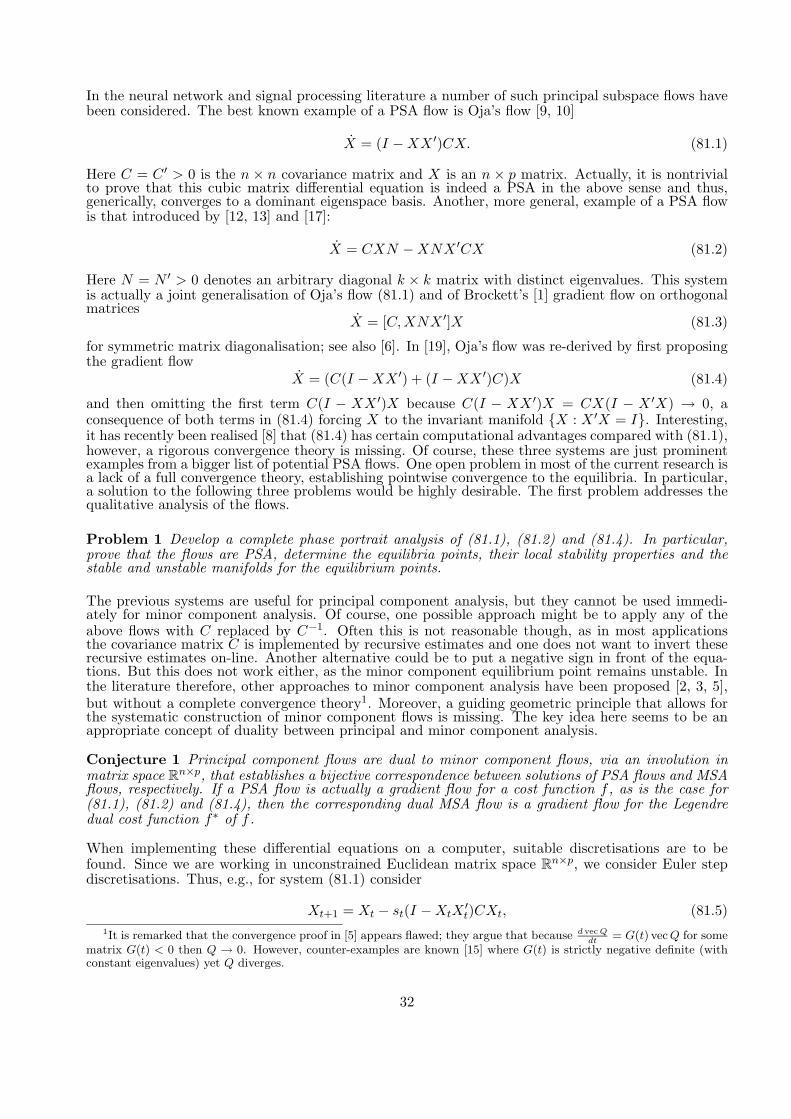
In the neural network and signal processing literature a number of such principal subspace flows havebeen considered. The best known example of a PSA flow is Oja’s flow [9, 10]

X = (I −XX ′)CX. (81.1)

Here C = C ′ > 0 is the n × n covariance matrix and X is an n × p matrix. Actually, it is nontrivialto prove that this cubic matrix differential equation is indeed a PSA in the above sense and thus,generically, converges to a dominant eigenspace basis. Another, more general, example of a PSA flowis that introduced by [12, 13] and [17]:

X = CXN −XNX ′CX (81.2)

Here N = N ′ > 0 denotes an arbitrary diagonal k × k matrix with distinct eigenvalues. This systemis actually a joint generalisation of Oja’s flow (81.1) and of Brockett’s [1] gradient flow on orthogonalmatrices

X = [C,XNX ′]X (81.3)

for symmetric matrix diagonalisation; see also [6]. In [19], Oja’s flow was re-derived by first proposingthe gradient flow

X = (C(I −XX ′) + (I −XX ′)C)X (81.4)

and then omitting the first term C(I − XX ′)X because C(I − XX ′)X = CX(I − X ′X) → 0, aconsequence of both terms in (81.4) forcing X to the invariant manifold X : X ′X = I. Interesting,it has recently been realised [8] that (81.4) has certain computational advantages compared with (81.1),however, a rigorous convergence theory is missing. Of course, these three systems are just prominentexamples from a bigger list of potential PSA flows. One open problem in most of the current research isa lack of a full convergence theory, establishing pointwise convergence to the equilibria. In particular,a solution to the following three problems would be highly desirable. The first problem addresses thequalitative analysis of the flows.

Problem 1 Develop a complete phase portrait analysis of (81.1), (81.2) and (81.4). In particular,prove that the flows are PSA, determine the equilibria points, their local stability properties and thestable and unstable manifolds for the equilibrium points.

The previous systems are useful for principal component analysis, but they cannot be used immedi-ately for minor component analysis. Of course, one possible approach might be to apply any of theabove flows with C replaced by C−1. Often this is not reasonable though, as in most applicationsthe covariance matrix C is implemented by recursive estimates and one does not want to invert theserecursive estimates on-line. Another alternative could be to put a negative sign in front of the equa-tions. But this does not work either, as the minor component equilibrium point remains unstable. Inthe literature therefore, other approaches to minor component analysis have been proposed [2, 3, 5],but without a complete convergence theory1. Moreover, a guiding geometric principle that allows forthe systematic construction of minor component flows is missing. The key idea here seems to be anappropriate concept of duality between principal and minor component analysis.

Conjecture 1 Principal component flows are dual to minor component flows, via an involution inmatrix space Rn×p, that establishes a bijective correspondence between solutions of PSA flows and MSAflows, respectively. If a PSA flow is actually a gradient flow for a cost function f , as is the case for(81.1), (81.2) and (81.4), then the corresponding dual MSA flow is a gradient flow for the Legendredual cost function f∗ of f .

When implementing these differential equations on a computer, suitable discretisations are to befound. Since we are working in unconstrained Euclidean matrix space Rn×p, we consider Euler stepdiscretisations. Thus, e.g., for system (81.1) consider

Xt+1 = Xt − st(I −XtX′t)CXt, (81.5)

1It is remarked that the convergence proof in [5] appears flawed; they argue that because d vecQdt

= G(t) vecQ for somematrix G(t) < 0 then Q → 0. However, counter-examples are known [15] where G(t) is strictly negative definite (withconstant eigenvalues) yet Q diverges.

32

with suitably small step sizes. Such Euler discretisation schemes are widely used in the literature, butusually without explicit step size selections that guarantee, for generic initial conditions, convergenceto the p dominant orthonormal eigenvectors of A. A further challenge is to obtain step size selectionsthat achieve quadratic convergence rates (e.g., via a Newton-type approach).

Problem 2 Develop a systematic convergence theory for discretisations of the flows, by specifyingstep-size selections that imply global as well as local quadratic convergence to the equilibria.

81.2 Motivation and History

Eigenvalue computations are ubiquitous in Mathematics and Engineering Sciences. In applications,the matrices whose eigenvectors are to be found are often defined in a recursive way, thus demandingrecursive computational methods for eigendecomposition. Subspace tracking algorithms are widelyused in neural networks, regression analysis and signal processing applications for this purpose. Sub-space tracking algorithms can be studied by replacing the stochastic, recursive algorithm through anaveraging procedure by a nonlinear ordinary differential equation. Similarly, new subspace trackingalgorithms can be developed by starting with a suitable ordinary differential equation and then con-verting it to a stochastic approximation algorithm [7]. Therefore, understanding the dynamics of suchflows is paramount to the continuing development of recursive eigendecomposition techniques.The starting point for most of the current work in principal component analysis and subspace trackinghas been Oja’s system from neural network theory. Using a simple Hebbian law for a single perceptronwith a linear activation function, Oja [9, 10] proposed to update the weights according to

Xt+1 = Xt − st(I −XtX′t)utu

′tXt. (81.6)

Here Xt denotes the n × p weight matrix and ut the input vector of the perceptron, respectively.By applying the ODE method to this system, Oja arrives at the differential equation (81.1). Here,C = E(utu′t) is the covariance matrix. Similarly, the other flows, (81.2) and (81.4), have analogousinterpretations.In [9, 11] it is shown for p = 1 that (81.1) is a PSA flow, i.e. it converges for generic initial conditionsto a normalised dominant eigenvector of C. In [11], the system (81.1) was studied for arbitrary valuesof p and it was conjectured that (81.1) is a PSA flow. This conjecture was first proven in [18], assum-ing positive definiteness of C. Moreover, in [18, 4], explicit initial conditions in terms of intersectiondimensions for the dominant eigenspace with the inital subspace were given, such that the flow con-verges to a basis matrix of the p-dimensional dominant eigenspace. This is reminiscent of Schuberttype conditions in Grassmann manifolds.Although the Oja flow serves as a principal subspace method, it is not useful for principal compo-nent analysis because it does not converge in general to a basis of eigenvectors. Flows for principalcomponent analysis such as (81.2) have been first studied in [14, 12, 13, 17]. However, pointwiseconvergence to the equilibria points was not established. In [16], a Lyapunov function for the Oja flow(81.1) was given, but without recognising that (81.1) is actually a gradient flow. There have been con-fusing remarks in the literature claiming that (81.1) cannot be a gradient system as the linearisationis not a symmetric matrix. However, this is due to a misunderstanding of the concept of a gradient.In [20] it is shown that (81.2), and in particular (81.1), is actually a gradient flow for the cost functionf(X) = 1/4tr(AXNX ′)2 − 1/2tr(A2XD2X ′) and a suitable Riemannian metric on Rn×p. Moreover,starting from any initial condition in Rn×p, pointwise convergence of the solutions to a basis of kindependent eigenvectors of A is shown together with a complete phase portrait analysis of the flow.First steps towards a phase portrait analysis of (81.4) are made in [8].

81.3 Available Results

In [12, 13, 17], the equilibrium points of (81.2) were computed together with a local stability analysis.Pointwise convergence of the system to the equilibria is established in [20] using an early result byLojasiewicz on real analytic gradient flows. Thus these results together imply that (81.2), and hence(81.1), is a PSA. An analogous result for (81.4) is forthcoming; see [8] for first steps in this direction.Sufficient conditions for initial matrices in the Oja flow (81.1) to converge to a dominant subspace

33

basis are given in [18, 4], but not for the other, unstable equilibria, nor for system (81.2). A completecharacterisation of the stable/unstable manifolds is currently unknown.

Bibliography

[1] R. W. Brockett. Dynamical systems that sort lists, diagonalise matrices, and solve linear pro-gramming problems. Linear Algebra Appl., 146:79–91, 1991.

[2] T. Chen. Modified Oja’s algorithms for principal subspace and minor subspace extraction. NeuralProcessing Letters, 5:105–110, April 1997.

[3] T. Chen, S. Amari, and Q. Lin. A unified algorithm for principal and minor component extraction.Neural Networks, 11:385–390, 1998.

[4] T. Chen, Y. Hua, and W.-Y. Yan. Global convergence of Oja’s subspace algorithm for principalcomponent extraction. IEEE Transactions on Neural Networks, 9(1):58–67, 1998.

[5] S. C. Douglas, S.-Y. Kung, and S. Amari. A self-stabilized minor subspace rule. IEEE SignalProcessing Letters, 5(12):328–330, December 1998.

[6] U. Helmke and J. B. Moore. Optimization and Dynamical Systems. Springer-Verlag, 1994.[7] H. J. Kushner and G. G. Yin. Stochastic Approximation Algorithms and Applications. Springer,

1997.[8] J. H. Manton, I. M. Y. Mareels, and S. Attallah. An analysis of the fast subspace tracking

algorithm NOja. In IEEE Conference on Acoustics, Speech and Signal Processing, Orlando,Florida, May 2002.

[9] E. Oja. A simplified neuron model as a principal component analyzer. Journal of MathematicalBiology, 15:267–273, 1982.

[10] E. Oja. Neural networks, principal components, and subspaces. International Journal of NeuralSystems, 1:61–68, 1989.

[11] E. Oja and J. Karhunen. On stochastic approximation of the eigenvectors and eigenvalues of theexpectation of a random matrix. Journal of Mathematical Analysis and Applications, 106:69–84,1985.

[12] E. Oja, H. Ogawa, and J. Wangviwattana. Principal component analysis by homogeneous neuralnetworks, Part I: The weighted subspace criterion. IEICE Transactions on Information andSystems, 3:366–375, 1992.

[13] E. Oja, H. Ogawa, and J. Wangviwattana. Principal component analysis by homogeneous neuralnetworks, Part II: Analysis and extensions of the learning algorithms. IEICE Transactions onInformation and Systems, 3:376–382, 1992.

[14] T. D. Sanger. Optimal unsupervised learning in a single-layer linear feedforward network. NeuralNetworks, 2:459–473, 1989.

[15] J. L. Willems. Stability theory of dynamical systems. Studies in dynamical systems. London,Nelson, 1970.

[16] J. L. Wyatt and I. M. Elfadel. Time-domain solutions of Oja’s equations. Neural Computation,7:915–922, 1995.

[17] L. Xu. Least mean square error recognition principle for self organizing neural nets. NeuralNetworks, 6:627–648, 1993.

[18] W.-Y. Yan, U. Helmke, and J. B. Moore. Global analysis of Oja’s flow for neural networks. IEEETransactions on Neural Networks, 5(5):674–683, September 1994.

[19] B. Yang. Projection approximation subspace tracking. IEEE Transactions on Signal Processing,43(1):95–107, January 1995.

[20] S. Yoshizawa, U. Helmke, and K. Starkov. Convergence analysis for principal component flows.International Journal of Applied Mathematics and Computer Science, 11:223–236, 2001.

34

Problem 55

Delta-Sigma Modulator Synthesis

Anders RantzerDept. of Automatic ControlLund Institute of TechnologyP.O. Box 118SE-221 00 LUNDSwedenrantzer@control.lth.se

55.1 Description of the problem

Delta-Sigma modulators are among the key components in modern electronics. Their main purposeis to provide cheap conversion from analog to digital signals. In the figure below, the analog signal rwith values in the interval [−1, 1] is supposed to be approximated by the digital signal d that takesonly two values, −1 and 1. One can not expect good approximation at all frequencies. Hence thedynamic system D should be chosen to minimize the error f in a given frequency range [ω1, ω2].

e Dynamicsystem D

-

−1

6

- --r f d

To make a more precise problem formulation, we need to introduce some notation:

Notation

The signal space `[0,∞] is the set of all sequences f(k)∞k=0 such that f(k) ∈ [−1, 1] for k = 0, 1, 2, . . ..A map D : `[0,∞] → `[0,∞] is called a causal dynamic system if for every u, v ∈ `[0,∞] such thatu(k) = v(k) for k ≤ T it holds that [D(u)](k) = [D(v)](k) for k ≤ T . Define also the static operator

sgn(x) =

1 if x ≥ 0−1 else

Problem

Given r ∈ `[0,∞] and a causal dynamic system D, define d, f ∈ `[0,∞] byd(k + 1) = sgn

([D(f)](k)

), d(0) = 0

f(k) = r(k)− d(k)

35

The problem is to find a D such that regardless of the reference input r, the error signal f becomessmall in a prespecified frequency interval [ω1, ω2].The problem formulation is intentionally left vague on the last line. The size of f can be measured inmany different ways. One option is to require a uniform bound on

lim supT→∞

1T

∣∣∣∣∣T∑k=0

e−ikωf(k)

∣∣∣∣∣for all ω ∈ [ω1, ω2] and all reference signals r ∈ `[0,∞].Another option is to allow D to be stochastic system and put a bound on the spectral density of fin the frequency interval. This would be consistent with the wide-spread practice to add a stochastic“dithering signal” before the nonlinearity in order to avoid undesired periodic orbits.

55.2 Available results

The simplest and best understood case is wherex(k + 1) = x(k) + f(k)f(k) = r(k)− sgn(x(k))

In this case, it is easy to see that the set x ∈ [−2, 2] is invariant, so with

FT (z) =T∑k=0

z−kf(k) XT (z) =T∑k=0

z−kx(k)

it holds that

1T

∫ ω0

0|FT (eiω)|2dω =

1T

∫ ω0

0|(eiω − 1)XT (eiω)|2dω

=1T

∫ ω0

0

[2(1− cosω)|XT (eiω)|2

]dω

≤ 2(1− cosω0)1T

∫ π

0|XT (eiω)|2dω

= 2(1− cosω0)π

T

T∑k=0

x(k)2

≤ 8π(1− cosω0)

which clearly bounds the error f at low frequencies.Many modifications using higher order dynamics have been suggested in order to further reduce theerror. However, there is still a strong demand for improvements and a better understanding of thenonlinear dynamics. The following two references are suggested as entries to the literature on ∆-Σ-modulators:

Bibliography

[1] James A. Cherry. Continuous time Delta-Sigma Modulators for High-speed A/D conversion: The-ory, Practice & Fundamental Performance Limits. Kluwer, 1999.

[2] S.R. Norsworthy, R. Schreier, and G.C. Temes. Delta-Sigma data converters. IEEE Press, NewYork, 1997.

36

Problem 44

Locomotive Drive Control by UsingHaar Wavelet Packets

P. MercorelliInstitut fur Automatisierung und Informatik GmbHZentrum fur Industrielle Forschung und EntwicklungSchlachthof 4 WernigerodeGermanypmercorelli@hs-harz.demercorelli@iai-wr.de

P. TerwieschABB Corporate ResearchSegelhof, CH-5405 BadenSwitzerlandPeter.Terwiesch@ch.abb.com

D. PrattichizzoDip. di Ingegneria dell’ Informazione – Universita di Sienavia Roma, 5653100 SienaItalyprattichizzo@ing.unisi.it

44.1 Description of the problem

Preliminary simulations and roughly algorithms show how the use of wavelet packets are very promisingin itermodulation disturbance rejection for converter bridge control. The presented contribution wantsto pay attention on an original way to states a possible converter bridge control by using Haar waveletpackets. The presented attack to the problem could represent a possible alternative to the traditionalPWM control for the converter bridge. The idea is to find an algorithm which guaranties the neededpower supply and in the meantime a high level of the S

N ratio. One proposes a roughly algorithmwhich find the length of the active switching function looking for suitable scaling function. The openproblem consists of checking the suitability of its formulation in order to build a rigorous algorithmwhich can find a switching control law.

44.2 Motivation and history of the problem

The modern vehicles produced during the past decade is radically different from previous generationsof vehicles. Power semiconductors, such as GTOs (gate turn-off thyristors) and IGBTs (insulated gatebipolar transistors) combined with computer control systems have greatly enhanced the functionalityof rail vehicles. New vehicles are now able to operate under different AC and DC supply networks withonly moderate additional equipment effort, which is essential when traveling over country borders. Itwas found on the overline of the rail system of several countries that particular disturbances, generated

37

by drive control, produce dangerous oscillation problems with resonance and sometimes instabilityphenomena, thus to recognize these particular frequencies and to actively suppress them is a necessaryand ambitious task. Classical PWM control is very sensitive to the level of the dc link voltage but itis not sensitive to the frequency disturbance in superposition.Theoretical aspect on wavelets are known already from many years [2] or [?] and in particular waveletpackets as in [1]. Nevertheless they industrial application have been recently presented. Recenttechnical publications see for instance [6], [10] pointed out how wavelet tools are particular suitablein order to describe power control problems and they gave already good results. There are in [5] and[4] significant contributions where the Haar functions are used in order to analyze electrical systems.More, very recent patents, see [7] and for instance [8], make clear the interest of the industry communityto invest on this area and indicate already a real possibility to apply with success wavelet packets.Preliminary simulations and theoretic considerations show a good chances to achieve several interestingresults connected to the applications as well as to theoretical aspects. The presented contribution isorganized as follows. In section 44.3 one states the problem in a mathematical form. In section 44.4preliminary simulation of a roughly idea of solution is shown and in the meantime one discusses somearising problems. At the end one comes to the conclusions.

44.3 General Problem Formulation

Given the following non linear system,

x(t) = f(x, t) + b(x, t)usw(t). (44.1)

Let the tracking error be x(t) ∈ < with

e(t) = x(t) = xw(t)− x(t),

where the xw(t) is the wanted function.Find a suitable usw(t), switching input function, such that ∀ t e(t) is as smaller as possible under thefollowing constraint condition on the system

C(x(t), x(t)

)= 0

44.3.1 A Conjecture in Converter Bridge Control

One can start with a particular linear time varying system characterized as follows:

x(t) = Ax(t) + B(Un(t)− Ud(t)usw(t)

), (44.2)

where the A and the B matrices are the maps of the linear system and Ud(t) could be interpreted likean external disturbances, usw(t) is a switching function. According to the preliminary model discussedin [9], the mathematical model becomes:

In(t) +R

LIn(t) =

1L

[Un(t)− Ud(t)usw(t)], (44.3)

where Un(t) is a sinusoidal feeding voltage and Ud(t) is the dc-link voltage, the disturbance is due tothe charge of the motor.In other words this system could be seen like a time-varying system. In order to ’localize’ the distur-bance, the problem is, roughly speaking, to find a switching function usw(t) such that the secondarycurrent of the transformer has sinousoidal shape depending only on the fundamental frequency andwith the same phase as the feeding voltage.One of the possible idea of the solution is the following.If

38

Ud(t) < V − 0.05V, (44.4)

where V is the required voltage level, thenfind a suitable level ”d” of the tree Haar wavelet functions such that

mind

(D(Iw(t), In(t)))1 (44.5)

and able to obtain ∫In(t)Ud(t)usw(t)d(t) ≥ 1

2CV 2. (44.6)

Where Iw(t) and In(t) are the secondary wanted and nominal current of the transformer, Ud(t) is thedc link voltage and the product CV is the required charge condition from the capacitor battery at thewanted voltage V . One can remark:

The condition (44.6) could be again easily interpreted as a distance condition to satisfy on the packettree. In other words, the problem is to be able to find a compatible solution.

Another important aspect to remark is how, thanks to the time-frequency localization of the waveletfunction, the problem of the phase shift of the signals is easily resolved by using the idea of the func-tional distance D.

About the constraint (44.6), one doesn’t risk a dangerous over voltage because the system is technicallyprotected from over tension.

44.4 Several Preliminary Simulations and Considerations

Preliminary simulations show how it exists an uws(t) control low such that the amplitude of the dis-turbances of intermodulation are often considerably reduced, even though the noise level is increased.The simulations have been performed with realistic values given from ADtranz, see [9]. One consideredfor the simulation

Iw(t) = xw(t) = 300cos(2π ∗ 50 ∗ t). (44.7)

The disturbance with frequency of 25 Hz and amplitude of around 100 A, this condition simulatesa possible start-in of the train. One can observe that the sincronismus is kept, in fact the maindisturbances, intermodulation disturbance, has frequencies equal to 25 Hz and 75 Hz, 50± 25.By using, a window with 8 samples then the levels of the packets are 3, a sampling time equal to 2 msthen tha analysing signal has length equal to 16 ms. Looking on the wavelet packet tree one can finda suitable level in order to find the length of the modulating input. In other words, the length of thescaling function corresponding to the selected level is the active wanted time of the switching wantedfunction. From the preliminary simulations one can see the two disturbances due to the modulationand how they are reduced from the proposed approach.Arising problems:

• Does exist, for every charge condition, in the set of ”d” levels, under the condition (44.6), asolution which guaranties the condition (44.5) ?

• If one considers more samples with the same sampling time then the number ”d” of the levels isincreased. Then, the set of the possible candidate functions is bigger, this yields more possibilitiesto find a suitable solution. But, a longer window increases the information on the past real timeaxis, this yields not necessarely a suitable solution.

• The level of the white noise is sensitively higher than with PWM pulse pattern.1Where with D one indicates one functional distance.

39

44.5 Conclusion

The contribution presents an original way to perform a converter bridge control by using waveletpackets and proposes a line of research to follow. The idea could be a possible alternative to the PWMcontrol in locomotive drive where one needs to have a high level of the S

N ratio. This preliminaryidea seems quite challenging and promising in order to guarantee the required power supply and agood power factor. One proposes a roughly algorithm which finds the length of the active switchingfunction looking for the suitable scaling function. The open problem consists of building a rigorousalgorithm which can find a switching control law.

Bibliography

[1] R. R Coifman and M. V. Wickerhauser, ”Entropy based algorithm for best basis selection”, IEEETrans. Inform. Theory,32,712-718,(1992).

[2] R. R. Coifman, Y. Meyer and M.V. Wickerhauser, ”Wavelet Analysis and Signal Processing”,Publisher Jones and Bartlett,Boston (USA), 153-178,(1992).

[3] I. Daubechies,”Ten Lectures on Wavelets”, Publisher Society for Industrial and Applied Mathe-matics, Philadelphia (Pennsylvania), (1995).

[4] A. Gandelli and A. Monti and F. Ponci and E. Santi, ”Power converter control design based onhaar analysis”, PESC. 2001 IEEE 32nd Annual Power Electronics Specialists Conference,3,1742-1746,(2001).

[5] , A. Gandelli and S. Leva,”Haar state equations for power electronics system modeling”, The 2001IEEE International Symposium on Circuits and Systems 2001 ISCAS 2001,2, 4525-528,(2001).

[6] P. Mercorelli and P. Terwiesch, ”A Black Box Identification in Harmonic Domain”, VDE EuropeanTransactions on Electrical Power, to appear 2002.

[7] P. Mercorelli and A. Frick, ”System and Methodology for Noise Level Detection by Using WaveletBasis Functions in Wavelet Packet Trees”, In Patentamt ABB Corporate Research Ladenburg(Germany),2002.

[8] , P. Mercorelli and A. Frick, ”System and Methodology for Gross Error Detection by Using WaveletBasis Functions in Wavelet Packet Trees”, In Patentamt ABB Corporate Research Ladenburg(Germany),(2002).

[9] , A. Petersen, ”Calculation Tools-Mathematical Background”, Thecnical Report, 3EHA610201 byADtranz, (1997).

[10] , P. Terwiesch, S. Menth and S. Schmidt, ” Analysis of Transients in Electrical Railway NetworksUsing Wavelets”, IEEE Trans. on Industrial Electronics, 45,6,955-959,(1998).

40

Problem 61

Determining of various asymptotics ofsolutions of nonlinear time-optimalproblems via right ideals in themoment algebra

G. M. SklyarSzczecin UniversityWielkopolska str. 15, 70-451 Szczecin, Poland;Kharkov National UniversitySvoboda sqr. 4, 61077 Kharkov, Ukraine¡mailto:sklar@sus.univ.szczecin.pl¿sklar@sus.univ.szczecin.pl, ¡mailto:sklyar@univer.kharkov.ua¿sklyar@univer.kharkov.ua

S. Yu. IgnatovichKharkov National UniversitySvoboda sqr. 4, 61077 Kharkov, Ukraine¡mailto:bob@online.kharkiv.com¿bob@online.kharkiv.com

61.1 Motivation and history of the problem

The time-optimal control problem is one of the most natural and at the same time hard problems inthe optimal control theory.For linear systems the maximum principle allows to indicate a class of optimal controls. However,the explicit form of the solution can be given only in a number of particular cases [1-3]. At the sametime [4] an arbitrary linear time-optimal problem with analytic coefficients can be approximated (ina neighborhood of the origin) by a certain linear problem of the form

xi = −tqiu, i = 1, . . . , n, q1 < · · · < qn, x(0) = x0, x(θ) = 0, |u| ≤ 1, θ → min . (1)

In the nonlinear case the careful analysis is required for any particular system [5,6]. However, in anumber of cases the time-optimal problem for a nonlinear system can be approximated by a linearproblem of the form (1) [7]. We recall this result briefly. Consider the time-optimal problem in thefollowing statement

x = a(t, x) + ub(t, x), a(t, 0) ≡ 0, x(0) = x0, x(θ) = 0, |u| ≤ 1, θ → min, (2)

where a, b are real analytic in a neighborhood of the origin in Rn+1. Let us denote by (θx0 , ux0) thesolution of this problem.Denote by Ra, Rb the operators acting as Rad(t, x) = dt(t, x) + dx(t, x) · a(t, x), Rbd(t, x) = dx(t, x) ·b(t, x) for any vector function d(t, x) analytic in a neighborhood of the origin in Rn+1 and let ad m+1

RaRb =

[Ra, admRaRb], m ≥ 0; ad 0RaRb = Rb, where [·, ·] is the operator commutator. Denote E(x) ≡ x.

41

Theorem 1. The conditions rankadjRaRbE(x)∣∣t=0x=0j≥0 = n and

[adm1RaRb, · · · [admk−1

RaRb, admkRaRb] · · · ]E(x)

∣∣t=0x=0∈ Lin

adjRaRbE(x)

∣∣t=0x=0

m−2

j=0(3)

for any k ≥ 2 and m1, . . . ,mk ≥ 0, where m = m1 + · · · + mk + k, hold if and only if there exista nonsingular transformation Φ of a neighborhood of the origin in Rn, Φ(0) = 0, and a linear time-optimal problem of the form (1) which approximates problem (2) in the following sense

θΦ(x0)

θLinx0

→ 1,1θ

∫ θ

0|uLinx0 (t)− uΦ(x0)(t)|dt→ 0 as x0 → 0,

where (θLinx0 , uLinx0 ) denotes the solution of (1) and θ = minθΦ(x0), θLinx0 .

That means that if the conditions of Theorem 1 are not satisfied then the asymptotic behavior ofthe solution of the nonlinear time-optimal problem differs from asymptotics of solutions of all linearproblems.In order to formulate the next result let us give the representation of the system in the form of a seriesof nonlinear power moments [7]. We assume the initial point x0 is steered to the origin in the time θby the control u(t) w.r.t. system (2). Then under our assumptions for rather small θ one has

x0 =∞∑m=1

∑m1+···+mk+k=m

vm1...mkξm1...mk(θ, u), (4)

where ξm1...mk(θ, u) =∫ θ

0

∫ τ10 · · ·

∫ τk−1

0

∏kj=1 τ

mjj u(τj) dτk · · · dτ2dτ1 are nonlinear power moments and

vm1...mk=(−1)k

m1! · · ·mk!adm1

RaRb adm2

RaRb · · · admkRaRbE(x)

∣∣t=0x=0

.

We say that ord(ξm1...mk) = m1 + · · ·+mk + k is the order of ξm1...mk .Theorem 1 means that there exists a transformation Φ which reduces (4) to

(Φ(x0))i = ξqi(θ, u) + ρi, i = 1, . . . , n,

where ρi includes power moments of order greater than qi+ 1 only while the representation (4) for thelinear system (1) obviously has the form

x0i = ξqi(θ, u), i = 1, . . . , n.

That is the linear moments which correspond to the linear time-optimal problem (1) form the principalpart of the series in representation (4) as θ → 0.When condition (3) is not satisfied one can try to find a nonlinear system which has rather simplyform and approximates system (2) in the sense of time optimality. In [8] we claim the following result.Consider the linear span A of all nonlinear moments ξm1...mk over R as a free algebra with the basisξm1...mk : k ≥ 1,m1, . . . ,mk ≥ 0 and the product ξm1...mkξn1...ns = ξm1...mkn1...ns . Introduce theinner product in A assuming the basis ξm1...mk to be orthonormal. Consider also the Lie algebraL over R generated by the elements ξm∞m=0 with the commutator [`1, `2] = `1`2 − `2`1. Introducefurther the graded structure A =

∑∞m=1 Am putting Am = Linξm1...mk : ord(ξm1...mk) = m.

Consider now a system of the form (2). The series in (4) naturally defines the linear mapping v :A → R

n by the rule v(ξm1...mk) = vm1...mk . Further we assume the system (2) to be n-dimensional,i.e. dim v(L) = n. Note that the form of coefficients vm1...mk of the series in (4) implies the followingproperty of the mapping v: the equality v(`) = 0 for ` ∈ L implies v(`x) = 0 for any x ∈ A. Thatmeans that any system of the form (2) generates a right ideal in the algebra A. We introduce theright ideal in the following way.

42

Consider the sequence of subspaces Dr = v(L∩ (A1 + · · ·+Ar)) ⊂ Rn, and put r0 = minr : dimDr =n. For any r ≤ r0 consider a subspace Pr of all elements y ∈ L ∩ Ar such that v(y) ∈ Dr−1 (weassume D0 = 0). Then put J =

∑r0r=1 Pr(A + R). Let J⊥ be the orthogonal complement of J . In

the next theorem LJ⊥ denotes the projection of the Lie algebra L on J⊥.

Theorem 2. (A) Let system (2) be n-dimensional, ˜1, . . . , ˜n be a basis of∑r0

r=1(LJ⊥ ∩ Ar) suchthat ord(˜i) ≤ ord(˜j) as i < j. Then there exists a nonsingular analytic transformation Φ of aneighborhood of the origin which reduces (4) to the following form

(Φ(x0))i = ˜i + ρi, i = 1, . . . , n,

where ρi contains moments of order greater than ord(˜i) only. Moreover, there exists a control systemof the form

x = ub∗(t, x), (5)

such that representation (4) for this system is of the form

x0i = ˜

i, i = 1, . . . , n. (6)

(B) Suppose there exists an open domain Ω ⊂ Rn\0, 0 ∈ Ω, such thati) the time-optimal problem for system (5) with representation (6) has a unique solution (θ∗x0 , u

∗x0(t))

for any x0 ∈ Ω;ii) the function θ∗x0 is continuous for x0 ∈ Ω;

iii) denote K = u∗x0(tθ∗x0) : x0 ∈ Ω and suppose that the following condition holds: when consideringK as a set in the space L2(0, 1), the weak convergence of a sequence of elements from K implies thestrong convergence.Then the time-optimal problem for system (5) approximates problem (2) in the domain Ω in thefollowing sense: there exists a set of pairs (θx0 , ux0(t)), x0 ∈ Ω, such that the control ux0(t) steers thepoint Φ(x0) to the origin in the time θx0 w.r.t. system (2) and

θΦ(x0)

θ∗x0

→ 1,θx0

θ∗x0

→ 1,1θ

∫ θ

0|u∗x0(t)− ux0(t)|dt→ 0 as x0 → 0, x0 ∈ Ω,

where θΦ(x0) is the optimal time for problem (2) and θ = minθx0 , θ∗x0.Remark 1. If there exists the autonomous system x = a(x) + ub(x) such that its representation (4)is of the form (6) and the origin belongs to the interior of the controllability set then the function θ∗x0

is continuous in a neighborhood of the origin [9]. Further, if time-optimal controls for system (5) arebang-bang then they satisfy condition iii) of Theorem 2.Remark 2. Consider any r0 ≥ 0 and an arbitrary sequence of subspaces M = Mrr0r=1, Mr ⊂ L∩Ar,such that

∑r0r=1(dim(L ∩ Ar) − dimMr) = n. Put JM =

∑r0r=1Mr(A + R). We denote by J the set

of all such ideals. For any J ∈ J one can construct a control system of the form (5) such that itsrepresentation (4) is of the form (6).

61.2 Formulation of the problem.

Thus, the steering problem x = a(t, x) + ub(t, x), x(θ) = 0, where a(t, 0) ≡ 0, generates the right idealin the algebra A, which defines system (5), and, under conditions i)–iii) of Theorem 2, describes theasymptotics of the solution of time-optimal problem (2). The question is: if any system of the form(5) having the representation of the form (6) satisfies conditions i)–iii) of Theorem 2.The positive answer means that all possible asymptotics of solutions of the time-optimalproblems (2) are represented as asymptotics of solutions of the time-optimal problemsfor systems (5) with representations of the form (6).

43

In the other words, if any system of the form (5) having the representation of the form (6) satisfiesconditions i)–iii) of Theorem 2 then time-optimal problems (2) induce the same structure in the algebraA as steering problems to the origin under the constraint |u| ≤ 1, namely, the set of right ideals J. Ifthis is not the case then the next problem is to describe constructively the class of such systems.

Bibliography

[1] V. I. Korobov and G. M. Sklyar, ”Time optimality and the power moment problem, Math. USSRSb., 62, pp. 185-205 (1989).

[2] V. I. Korobov and G. M. Sklyar, ”Time optimality and the trigonometric moment problem, Math.USSR Izv., 35, pp. 203-220 (1990).

[3] V. I. Korobov and G. M. Sklyar, ”Markov power min-problem with periodic gaps”, J. Math. Sci.,80 , pp. 1559-1581 (1996).

[4] G. M. Sklyar and S. Yu. Ignatovich, ”A classification of linear time-optimal control problems in aneighborhood of the origin”, J. Math. Anal. Applic., 203, pp. 791-811 (1996).

[5] A. Bressan, ”The generic local time-optimal stabilizing controls in dimension 3”, SIAM J. ControlOptimiz., 24, pp. 177-190 (1986).

[6] B. Bonnard, ”On singular estremals in the time minimal control problem in R3”, SIAM J. ControlOptimiz., 23, pp. 794-802 (1985).

[7] G. M. Sklyar and S. Yu. Ignatovich, ”Moment approach to nonlinear time optimality”, SIAM J.Control Optimiz., 38, pp. 1707-1728 (2000).

[8] G. M. Sklyar and S. Yu. Ignatovich, ”Approximation in the sense of time optimality via nonlinearmoment problems”, submitted to SIAM J. Control Optimiz.

[9] V. I. Korobov, ”On continuous dependence of the solution of the optimal control problem withfree time on initial data”, Differen. Uravn., 7, pp. 1120-1123 (1971) (in Russian).

44

Problem 28

L2-Induced Gains of Switched LinearSystems

Joao P. Hespanha1

Dept. Electrical and Computer Engineering,University of California, Santa BarbaraUSAhespanha@ece.ucsb.edu

In the 1999 collection of Open Problems in Mathematical Systems and Control Theory weproposed the problem of computing input-output gains of switched linear systems. Recentdevelopments provided new insights into this problem leading to new questions.

28.1 Switched Linear Systems

A switched linear system is defined by a parameterized family of realizations (Ap, Bp, Cp, Dp) : p ∈ P,together with a family of piecewise constant switching signals S := σ : [0,∞)→ P. Here, we considerswitched systems for which all the matrices Ap, p ∈ P are Hurwitz. The corresponding switched systemis represented by

x = Aσx+Bσu, y = Cσx+Dσu, σ ∈ S (28.1)

and by a solution to (28.1), we mean a pair (x, σ) for which σ ∈ S and x is a solution to the time-varyingsystem

x = Aσ(t)x+Bσ(t)u, y = Cσ(t)x+Dσ(t)u, t ≥ 0. (28.2)

Given a set of switching signals S, we define the L2-induced gain of (28.1) by

infγ ≥ 0 : ‖y‖2 ≤ γ‖u‖2, ∀u ∈ L2, x(0) = 0, σ ∈ S,

where y is computed along solutions to (28.1). The L2-induced gain of (28.1) can be viewed as a“worst-case” energy amplification gain for the switched system, over all possible inputs and switchingsignals and is an important tool to study the performance of switched systems, as well as the stabilityof interconnections of switched systems.

28.2 Problem Description

We are interested here in families of switching signals for which consecutive discontinuities are sep-arated by no less than a positive constant called the dwell-time. For a given τD > 0, we denote by

1This material is based upon work supported by the National Science Foundation under Grant No. ECS-0093762.

45

S[τD] the set of piecewise constant switching signals with interval between consecutive discontinu-ities no smaller than τD. The general problem that we propose is the computation of the functiong : [0,∞) → [0,∞] that maps each dwell-time τD with the L2-induced gain of (28.1), for the set ofdwell-time switching signals S := S[τD]. Until recently little more was known about g other than thefollowing:

1. g is monotone decreasing

2. g is bounded below by

gstatic := supp∈P‖Cp(sI −Ap)−1Bp +Dp‖∞,

where ‖T‖∞ := sup<[s]≥0 ‖T (s)‖ denotes the H∞-norm of a transfer matrix T . We recall that‖T‖∞ is numerically equal to the L2-induced gain of any linear time-invariant system withtransfer matrix T .

Item 1 is a trivial consequence of the fact that given two dwell-times τD1 ≤ τD2 , we have thatS[τD1 ] ⊃ S[τD2 ]. Item 2 is a consequence of the fact that every set S[τD], τD > 0 contains all theconstant switching signals σ = p, p ∈ P. It was shown in [2] that the lower-bound gstatic is strict andin general there is a gap between gstatic and

gslow := limτD→∞

g[τD].

This means that even switching arbitrarily seldom, one may not be able to recover the L2-inducedgains of the “unswitched systems.” In [2], a procedure was given to compute gslow. Opposite to whathad been conjectured, gslow is realization dependent and cannot be determined just from the transferfunctions of the systems being switched.

The function g thus looks roughly like the ones shown in Figure 28.1, where (a) corresponds to a set ofrealizations that remains stable for arbitrarily fast switching and (b) to a set that can exhibit unstablebehavior for sufficiently fast switching [3]. In (b), the scalar τmin denotes the smallest dwell-time forwhich instability can occur for some switching signal in S[τmin].

gstatic

gslow

τD

g(τD)

gstatic

gslow

g(τD)

τDτmin

(a) (b)

Figure 28.1: L2-induced gain versus the dwell-time.

Several important basic question remain open:

1. Under what conditions is g bounded? This is really a stability problem whose general solutionhas been eluding researchers for a while now (cf., the survey paper [3] and references therein).

2. In case g is unbounded (case (b) in Figure 28.1), how to compute the position of the verti-cal asymptote? Or equivalently, what is the smallest dwell-time τmin for which one can haveinstability.

3. Is g a convex function? Is it smooth (or even continuous)?

Even if direct computation of g proves to be difficult, answers to the previous questions may provideindirect methods to compute tight bounds for it. They also provide a better understanding of thetrade-off between switching speed and induced gain. As far as we known, currently only very courseupper-bounds for g are available. These are obtained by computing a conservative upper-bound τupper

for τmin and then an upper-bound for g that is valid for every dwell-time larger than τupper (cf., e.g.,[4, 5]). These bounds do not really address the trade-off mentioned above.

46

Bibliography

[1] J. P. Hespanha and A. S. Morse, “Input-output gains of switched linear systems,” in Open Problemsin Mathematical Systems Theory and Control (V. D. Blondel, E. D. Sontag, M. Vidyasagar, andJ. C. Willems, eds.), London: Springer-Verlag, 1999.

[2] J. P. Hespanha, “Computation of root-mean-square gains of switched linear systems.” To be pre-sented at the Fifth Hybrid Systems: Computation and Control Workshop., Mar. 2002.

[3] D. Liberzon and A. S. Morse, “Basic problems in stability and design of switched systems,” IEEEContr. Syst. Mag., vol. 19, pp. 59–70, Oct. 1999.

[4] J. P. Hespanha and A. S. Morse, “Stability of switched systems with average dwell-time,” inProc. of the 38th Conf. on Decision and Contr., pp. 2655–2660, Dec. 1999.

[5] G. Zhai, B. Hu, K. Yasuda, and A. N. Michel, “Disturbance attenuation properties of time-controlled switched systems.” Submitted to publication., 2001.

47

Problem 48

Is Monopoli’s Model ReferenceAdaptive Controller Correct?

A. S. Morse 1

Center for Computational Vision and ControlDepartment of Electrical EngineeringYale University, New Haven, CT 06520 USA.

48.1 Introduction

In 1974 R. V. Monopoli published a paper [1] in which he posed the now classical model referenceadaptive control problem, proposed a solution and presented arguments intended to establish thesolution’s correctness. Subsequent research [2] revealed a flaw in his proof which placed in doubt thecorrectness of the solution he proposed. Although provably correct solutions to the model referenceadaptive control problem now exist see [3] and the references therein, the problem of decidingwhether or not Monopoli’s original proposed solution is in fact correct remains unsolved. The aimof this note is to review the formulation of the classical model reference adaptive control problem, todescribe Monopoli’s proposed solution, and to outline what’s known at present about its correctness.

48.2 The Classical Model Reference Adaptive Control Problem

The classical model reference adaptive control problem is to develop a dynamical controller capable ofcausing the output y of an imprecisely modelled siso process P to approach and track the output yrefof a pre-specified reference model Mref with input r. The underlying assumption is that the processmodel is known only to the extent that it is one of the members of a pre-specified class M. In theclassical problem M is taken to be the set of all siso controllable, observable linear systems with strictlyproper transfer functions of the form g β(s)

α(s) where g is a nonzero constant called the high frequencygain and α(s) and β(s) are monic, coprime polynomials. All g have the same sign and each transferfunction is minimum phase i.e., each β(s) is stable. All transfer functions are required to have thesame relative degree n i.e., degα(s) − deg β(s) = n. and each must have a McMillan degree notexceeding some pre-specified integer n i.e., degα(s) ≤ n. In the sequel we are going to discuss asimplified version of the problem in which all g = 1 and the reference model transfer function is of theform 1

(s+λ)n where λ is a positive number. Thus Mref is a system of the form

yref = −λyref + cxref + dr xref = Axref + br (48.1)

where A, b, c, d is a controllable, observable realization of 1(s+λ)(n−1) .

48

48.3 Monopoli’s Proposed Solution

Monopoli’s proposed solution is based on a special representation of P which involves picking anyn-dimensional, single-input, controllable pair (A, b) with A stable. It is possible to prove [1, 4] thatthe assumption that the process P admits a model in M, implies the existence of a vector p∗ ∈ IR2n

and initial conditions z(0) and x(0), such that u and y exactly satisfy

z =[A 00 A

]z +

[b0

]y +

[0b

]u

˙x = Ax+ b(u− z′p∗)y = −λy + cx+ d(u− z′p∗)

Monopoli combined this model with that of Mref to obtain the direct control model reference parame-terization

z =[A 00 A

]z +

[b0

]y +

[0b

]u (48.2)

x = Ax+ b(u− z′p∗ − r) (48.3)eT = −λeT + cx+ d(u− z′p∗ − r) (48.4)

Here eT is the tracking erroreT

∆= y − yref (48.5)

and x ∆= x−xref . Note that it is possible to generate an asymptotically correct estimate z of z using acopy of (48.2) with z replacing z. To keep the exposition simple we’re going to ignore the exponentiallydecaying estimation error z − z and assume that z can be measured directly.To solve the MRAC problem, Monopoli proposed a control law of the form

u = z′p+ r (48.6)

where p is a suitably defined estimate of p∗. Motivation for this particular choice stems from the factthat if one knew p∗ and were thus able to use the control u = z′p∗ + r instead of (48.6), then thiswould cause eT to tend to zero exponentially fast and tracking would therefore be achieved.Monopoli proposed to generate p using two sub-systems which we will refer to here as a “multi-estimator” and a “ tuner” respectively. A multi-estimator E(p) is a parameter-varying linear systemwith parameter p, whose inputs are u, y and r and whose output is an estimate e of eT which would beasymptotically correct were p held fixed at p∗. It turns out that there are two different but very similartypes of multi-estimators which have the requisite properties. While Monopoli focused on just one,we will describe both since each is relevant to the present discussion. Both multi-estimators contain(48.2) as a sub-system.

48.3.1 Version 1

There are two versions of the adaptive controller which a relevant to the problem at hand. In thissection we describe the multi-estimator and tuner which together with reference model (48.1) andcontrol law (48.6), comprise the first version.

Multi-Estimator 1

The form of the first multi-estimator E1(p) is suggested by the readily verifiable fact that if H1 andw1 are n× 2n and n× 1 signal matrices generated by the equations

H1 = AH1 + bz′ and w1 = Aw1 + b(u− r) (48.7)

respectively, then w1 −H1p∗ is a solution to (48.3). In other words x = w1 −H1p

∗ + ε where ε is aninitial condition dependent time function decaying to zero as fast as eAt. Again for simplicity we shallignore ε. This means that (48.4) can be re-written as

eT = −λeT − (cH1 + dz′)p∗ + cw1 + d(u− r)

49

Thus a natural way to generate an estimate e1 of eT is by means of the equation

˙e1 = −λe1 − (cH1 + dz′)p+ cw1 + d(u− r) (48.8)

From this it clearly follows that the multi-estimator E1(p) defined by (48.2), (48.7) and (48.8) has therequired property of delivering an asymptotically correct estimate e1 of eT if p is fixed at p∗.

Tuner 1

From (48.8) and the differential equation for eT directly above it, it can be seen that the estimationerror2

e1∆= e1 − eT (48.9)

satisfies the error equatione1 = −λe1 + φ′1(p− p∗) (48.10)

whereφ′1 = −(cH1 + dz′) (48.11)

Prompted by this, Monopoli proposed to tune p1 using the pseudo-gradient tuner

˙p1 = −φ1e1 (48.12)

The motivation for considering this particular tuning law will become clear shortly, if it is not already.

What’s Known About Version 1?

The overall model reference adaptive controller proposed by Monopoli thus consists of the referencemodel (48.1), the control law (48.6), the multi-estimator (48.2), (48.7), (48.8), the output estimationerror (48.9) and the tuner (48.11), (48.12). The open problem is to prove that this controller eithersolves the model reference adaptive control problem or that it does not.Much is known which is relevant to the problem. In the first place, note that (48.1), (48.2) together with(48.5) - (48.11) define a parameter varying linear system Σ1(p) with input r, state yref , xref , z,H1, w1,e1, e1 and output e1. The consequence of the assumption that every system in M is minimum phaseis that Σ1(p) is detectable through e1 for every fixed value of p [5]. Meanwhile the form of (48.10)enables one to show by direct calculation, that the rate of change of the partial Lyapunov functionV

∆= e21 + ||p− p∗||2 along a solution to (48.12) and the equations defining Σ1(p), satisfies

V = −2λe21 ≤ 0 (48.13)

From this it is evident that V is a bounded monotone nonincreasing function and consequently thate1 and p are bounded wherever they exist. Using and the fact that Σ1(p) is a linear parameter-varying system, it can be concluded that solutions exist globally and that e1 and p are bounded on[0,∞). By integrating (48.13) it can also be concluded that e1 has a finite L2[0,∞)-norm and that||e1||2 + ||p− p∗||2 tends to a finite limit as t→∞. Were it possible to deduce from these propertiesthat p tended to a limit p , then it would possible to establish correctness of the overall adaptivecontroller using the detectability of Σ1(p).There are two very special cases for which correctness has been established. The first is when theprocess models in M all have relative degree 1; that is when n = 1. See the references cited in [3] formore on this special case. The second special case is when p∗ is taken to be of the form q∗k where kis a known vector and q∗ is a scalar; in this case p ∆= qk where q is a scalar parameter tuned by theequation ˙q = −k′φ1e1 [6].

2Monopoli called e1 an augmented error.

50

48.3.2 Version 2

In the sequel we describe the multi-estimator and tuner which together with reference model (48.1)and control law (48.6), comprise the second version of them adaptive controller relevant to the problemat hand.

Multi-Estimator 2

The second multi-estimator E2(p) which is relevant to the problem under consideration, is similar toE1(p) but has the slight advantage of leading to a tuner which is somewhat easier to analyze. Todescribe E2(p), we need first to define matrices

A2∆=[A 0c −λ

]and b2

∆=[bd

]The form of E2(p) is motivated by the readily verifiable fact that if H2 and w2 are (n + 1) × 2n and(n+ 1)× 1 signal matrices generated by the equations

H2 = A2H2 + b2z′ and w2 = A2w2 + b2(u− r) (48.14)

then w2−H2p∗ is a solution to (48.3) - (48.4). In other words, [ x′ eT ]′ = w2−H2p

∗+ ε where ε isan initial condition dependent time function decaying to zero as fast as eA2t. Again for simplicity weshall ignore ε. This means that

eT = c2w2 − c2H2p∗

where c2 = [ 0 · · · 0 1 ]. Thus in this case a natural way to generate an estimate e2 of eT is bymeans of the equation

e2 = c2w2 − c2H2p (48.15)

It is clear that the multi-estimator E2(p) defined by (48.2), (48.14) and (48.15) has the requiredproperty of delivering an asymptotically correct estimate e2 of eT if p is fixed at p∗.

Tuner 2

Note that in this case the estimation error

e2∆= e2 − eT (48.16)

satisfies the error equatione2 = φ′2(p2 − p∗) (48.17)

whereφ′2 = −c2H2 (48.18)

Equation (48.17) suggests that one consider a pseudo-gradient tuner of the form

˙p = −φ2e2 (48.19)

What’s Known About Version 2?

The overall model reference adaptive controller in this case, thus consists of the reference model (48.1),the control law (48.6), the multi-estimator (48.2), (48.14), (48.15), the output estimation error (48.16)and the tuner (48.18), (48.19). The open problem is here to prove that this version of the controllereither solves the model reference adaptive control problem or that it does not.Much is known about the problem. In the first place, (48.1), (48.2) together with (48.5), (48.6) (48.14)- (48.18) define a parameter varying linear system Σ2(p) with input r, state yref , xref , z,H2, w2 andoutput e2. The consequence of the assumption that every system in M is minimum phase is that thisΣ2(p) is detectable through e2 for every fixed value of p [5]. Meanwhile the form of (48.17) enables one

51

to show by direct calculation, that the rate of change of the partial Lyapunov function V ∆= ||p− p∗||2along a solution to (48.19) and the equations defining Σ2(p), satisfies

V = −2λe22 ≤ 0 (48.20)

It is evident that V is a bounded monotone nonincreasing function and consequently that p is boundedwherever they exist. From this and the fact that Σ2(p) is a linear parameter-varying system, it canbe concluded that solutions exist globally and that p is bounded on [0,∞). By integrating (48.20) itcan also be concluded that e2 has a finite L2[0,∞)-norm and that ||p− p∗||2 tends to a finite limit ast→∞. Were it possible to deduce from these properties that p tended to a limit p , then it would toestablish correctness using the detectability of Σ2(p).There is one very special cases for which correctness has been established [6]. This is when p∗ is takento be of the form q∗k where k is a known vector and q∗ is a scalar; in this case p ∆= qk where q is ascalar parameter tuned by the equation ˙q = −k′φ2e2. The underlying reason why things go through isbecause in this special case, the fact that ||p− p∗||2 and consequently ||q − q∗|| tend to a finite limits,means that q tends to a finite limit as well.

48.4 The Essence of the Problem

In this section we write down a stripped down version of the problem which retains all the essentialfeature which need to be overcome in order to decide whether or not Monopoli’s controller is correct.We do this only for version 2 of the problem and only for the case when r = 0 and n = 1. Thus inthis case we can take A2 = −λ and b2 = 1. Assuming the reference model is initialized at 0, droppingthe subscript 2 throughout, and writing φ′ for −H, the system to be analyzed reduces to

z =[A 00 A

]z +

[b0

](w + φ′p∗) +

[0b

]p′z (48.21)

φ = −λφ− z (48.22)w = −λw + p′z (48.23)e = φ′(p− p∗) (48.24)˙p = −φe (48.25)

To recap, p∗ is unknown and constant but is such that the linear parameter-varying system Σ(p)defined by (48.21) to (48.24) is detectable through e for each fixed value of p. Solutions to the system(48.21) - (48.25) exist globally. The parameter vector p and integral square of e are bounded on [0,∞)and ||p−p∗|| tends to a finite limit as t→∞. The open problem here is to show for every initializationof (48.21)-(48.25), that the state of Σ(p) tends to 0 or that it does not.

Bibliography

[1] R. V. Monopoli. Model reference adaptive control with an augmented error. IEEE Transactionson Automatic Control, pages 474–484, October 1974.

[2] A. Feuer, B. R. Barmish, and A. S. Morse. An unstable system associated with model referenceadaptive control. IEEE Transactions on Automatic Control, 23:499–500, 1978.

[3] A. S. Morse. Overcoming the obstacle of high relative degree. European Journal of Control,2(1):29–35, 1996.

[4] K. J. Astrom and B. Wittenmark. On self-tuning regulators. Automatica, 9:185–199, 1973.[5] A. S. Morse. Towards a unified theory of parameter adaptive control - part 2: Certainty equivalence

and implicit tuning. IEEE Transactions on Automatic Control, 37(1):15–29, January 1992.[6] A. Feuer. Adaptive Control of Single Input Single Output Linear Systems. PhD thesis, Yale

University, 1978.

52

Problem 82

Stability of a Nonlinear AdaptiveSystem for Filtering and ParameterEstimation

Masoud Karimi-GhartemaniDepartment of Electrical and Computer EngineeringUniversity of TorontoToronto, Ontario, Canada M5S 3G4masoud@ele.utoronto.ca

Alireza K. ZiaraniDepartment of Electrical and Computer EngineeringClarkson UniversityPotsdam, NY, USA 13699-5720ziarani@ieee.org

82.1 Description of the problem

We are concerned about the mathematical properties of the dynamical system presented by the fol-lowing three differential equations:

dAdt = −2µ1A sin2φ+ 2µ1 sinφ f(t),

dωdt = −µ2A

2 sin(2φ) + 2µ2A cosφ f(t),

dφdt = ω + µ3

dωdt

(82.1)

where parameters µi, i = 1, 2, 3 are positive real constants and f(t) is a function of time having ageneral form of

f(t) = Ao sin(ωot+ δo) + f1(t). (82.2)

Ao, ωo and δo are fixed quantities and it is assumed that f1(t) has no frequency component at ωo.Variables A and ω are in R1 and φ varies on the one-dimensional circle S1 with radius 2π.The dynamical system presented by (82.1) is designed to (i) take the signal f(t) as its input signaland extract the component fo(t) = Ao sin(ωot + δo) as its output signal, and (ii) estimate the basicparameters of the extracted signal fo(t), namely its amplitude, phase and frequency. The extractedsignal is y = A sinφ and the basic parameters are the amplitude A, frequency ω and phase angleφ = ωt+ δ.Consider the three variables (A,ω, φ) in the three-dimensional space R1 × R1 × S1. The sinusoidalfunction fo(t) = Ao sin(ωot+ δo) corresponds to the To-periodic curve

Γo(t) = (Ao, ωo, ωot+ δo) (82.3)

53

in this space, with To = 2πωo

.

The following theorem, which the authors have proved in [1], presents some of the mathematicalproperties of the dynamical system presented by 82.1.Theorem 1: Consider the dynamical system presented by the set of ordinary differential equations(82.1) in which the function f(t) is defined in (82.2) and f1(t) is a bounded T1-periodic function withno frequency component at ωo. The three variables (A,ω, φ) are in R1 × R1 × S1. The parametersµi, i = 1, 2, 3 are small positive real numbers. If T1 = To

n for any arbitrary n ∈ N, the dynamicalsystem of (82.1) has a stable To-periodic orbit in a neighborhood of Γo(t) as defined in (82.3).The behavior of the system, as examined within the simulation environments, has led the authors tothe following two conjectures, the proofs of which are desired.Conjecture 1: With the same assumptions as those presented in Theorem 1, if T1 = p

qTo for anyarbitrary (p, q) ∈ N2 with (p, q) = 1, the dynamical system presented by (82.1) has a stable mTo-periodic orbit which lies on a torus in a neighborhood of Γo(t) as defined in (82.3). The value ofm ∈ N is determined by the pair (p, q).Conjecture 2: With the same assumptions as those presented in Theorem 1, if T1 = αTo for irrationalα, the dynamical system presented by (82.1) has an attractor set which is a torus in a neighborhoodof Γo(t) as defined in (82.3). In other words, the response is a never closing orbit which lies on thetorus. Moreover, this orbit is a dense set on the torus.For both conjectures, the neighborhood in which the torus is located depends on the values of param-eters µi, i = 1, 2, 3 and the function f1(t). If the function f1(t) is small in order and the parametersare properly selected, the neighborhood can be made to be very small, meaning that the filtering andestimation processes may be achieved with a high degree of accuracy.Theorem 1 deals with the local stability analysis of the dynamical system (82.1). In other words, theexistence of an attractor (periodic orbit or torus) and an attraction domain around the attractor isproved. However, this theorem does not deal with this domain of attraction. It is desirable to specifythis domain of attraction in terms of the function f1(t) and parameters µi, i = 1, 2, 3, hence thefollowing open problem:Open Problem: Consider the dynamical system presented by the ordinary differential equations(82.1) in which the function f(t) is defined in (82.2) and f1(t) is a bounded T1-periodic function withno frequency component at ωo. Three variables (A,ω, φ) are in R1×R1×S1. Parameters µi, i = 1, 2, 3are small positive real numbers. This system has an attractor set which may be either a periodic orbitor a torus based on the value of T1. It is desired to specify the extent of the attraction domain associatedwith the attractor in terms of the function f1(t) and the parameters µi, i = 1, 2, 3. In other words,and in a simplified case, for a three-parameter representation of f1(t) as f1(t) = a1 sin(2π/T1t + δ1),it is desirable to determine the whole region of points (A,ω, φ) in R1 × R1 × S1 which falls in theattraction domain of the attractor.

82.2 Motivation and history of the problem

The dynamical system presented by (82.1) was proposed by the authors for the first time [1, 2].The primary motivation was to devise a system for the extraction of a sinusoidal component withtime-varying parameters when it is corrupted by other sinusoids and noise. This is of significantinterest in power system applications, for instance [3]. Estimation of the basic parameters of theextracted sinusoid, namely the amplitude, phase and frequency, was another object of the work.These parameters provide important information useful in electrical engineering applications. Someapplications of the system in biomedical engineering are presented in [2, 4]. This dynamical systempresents an alternative structure for the well-known phase-locked loop (PLL) system with significantlyadvantageous features [5].

82.3 Available results

Theorem 1, corresponding to the case of T1 = Ton , has been proved by the authors in [1] where the

existence, local uniqueness and stability of a To-periodic orbit are shown using the Poincare map

54

theorem as stated in [6, page 70]. Extensive computer simulations verified by laboratory experimentalresults are presented in [1, 2, 5]. Some of the wide-ranging applications of the dynamical systemare presented in [2, 3, 4]. The algorithm governed by the proposed dynamical system presents apowerful signal processing method of analysis/synthesis of nonstationary signals. Alternatively, itmay be thought of as a nonlinear adaptive notch filter capable of estimation of parameters of theoutput signal.

Bibliography

[1] M. Karimi-Ghartemani and A.K. Ziarani, “Periodic Orbit Analysis of Two Dynamical Systems forElectrical Engineering Applications”, accepted for publication in International Journal of Engi-neering Mathematics.

[2] A.K. Ziarani, Extraction of Nonstationary Sinusoids, Ph.D. Dissertation, University of Toronto(2002).

[3] M. Karimi-Ghartemani and M.R. Iravani, “A Nonlinear Adaptive Filter for On-Line Signal Analysisin Power Systems: Applications”, IEEE Transactions on Power Delivery, 17, pp. 617-622 (2002).

[4] A.K. Ziarani and A. Konrad, “A Nonlinear Adaptive Method of Elimination of Power Line Inter-ference in ECG Signals”, IEEE Transactions on Biomedical Engineering, 49, pp. 540-547 (2002).

[5] M. Karimi-Ghartemani and M.R. Iravani, “An Alternative Structure for Phase-Locked Loop (PLL)System”, submitted to IEEE Transactions on Circuits and Systems I: Fundamental Theory andApplications.

[6] S. Wiggins, Introduction to Applied Nonlinear Dynamical Systems and Chaos, New York: Springer-Verlag (1983).

55

Problem 70

Decentralized Control withCommunication between Controllers

Jan H. van SchuppenCWIP.O. Box 94079, 1090 GB Amsterdam,The NetherlandsJ.H.van.Schuppen@cwi.nl

70.1 Description of the problem

At the request of Vincent Blondel, the following control problem has been formulated.

Problem - Decentralized control with communication between controllers Consider a con-trol system with inputs from r different controllers. Each controller has partial observations of thesystem and the partial observations of each pair of controllers is different. The controllers are allowedto exchange on-line information on their partial observations, state estimates, or input values but theirare constraints on the communication channels between each tuple of controllers. In addition, thereis specified a control objective.The problem is to synthesize r controllers and a communication protocol for each directed tuple ofcontrollers, such that when the controllers all use their received communications the control objectiveis met as well as possible.The problem can be considered for a discrete-event system in the form of a generator, for a timeddiscrete-event system, for a hybrid system, for a finite-dimensional linear system, for a finite-dimensionalGaussian system, etc. In each case the communication constraint has to be chosen and a formulationhas to be proposed on how to integrate the received communications into the controller.

Remarks on problem (1) The constraints on the communication channels between controllers areessential to the problem. Without it, every controller communicates all his/her partial observations toall other controllers and one obtains a control problem with a centralized controller, albeit one whereeach controller carries out the same control computations.(2) The complexity of the problem is large, for control of discrete-event systems it is likely to be unde-cidable. Therefore the problem formulation has to be restricted. Note that the problem is analogousto human communication in groups, firms, and organizations and that the communication problems insuch organizations are effectively solved on a daily basis. Yet, there is scope for a fundamental studyof this problem also for engineering control systems. The approach to the problem is best focused onthe formulation and analysis of simple control laws and on the formulation of necessary conditions.(3) The basic underlying problem seems to be: What information of a controller is so essential inregard to the control purpose that it has to be communicated to other controllers? A system theoreticapproach is suitable for this.(4) The problem will also be useful for the development of hierarchical models. The information tobe communicated has to be dealt with at a global level, the information that does not need to becommunicated can be treated at the local level.To assist the reader with the understanding of the problem, the special cases for discrete-event systems

56

and for finite-dimensional linear systems are stated below.

Problem - Decentralized control of a discrete-event system with communication betweensupervisors Consider a discrete-event system in the form of a generator and r supervisors,

G = (Q,E, f, q0), L(G) = s ∈ E∗|f(q0, s) is defined,∀k ∈ Zr, a partition, E = Ec,k ∪ Euc,k, Ecp,k = Es ⊆ E|Es ⊆ Ecp,k,∀k ∈ Zr, a partition, E = Eo,k ∪ Euo,k, pk : E → Eo,k, ∀k ∈ Zr,an event is enabled only if it is enabled by all supervisors,vk : pk(L(G))→ Ecp,k,∀k ∈ Zr,the set of supervisors based on partial observations,Lr, La ⊆ L(G), required and admissable language, respectively.

A variant of the problem is to determine a set of subsets of the event set which represent the eventsto be communicated by each supervisor to the other supervisors and a set of supervisors such that theclosed-loop system satisfies,

∀(i, j) ∈ Zr × Zr, Eo,i,j ⊆ Eo,i, pi,j : E → Eo,i,j ,

vk(pk(s), p1,k(s), . . . , pr,k(s)) 7→ Ecp,k,∀k ∈ Zr,the set of supervisors based on partial observations and on communications,L(v1 ∧ . . . ∧ vr/G) ⊆ La, ‘the closed-loop language, such that,

Lr ⊆ L(v1 ∧ . . . ∧ vr/G) ⊆ La, and the controlled system is nonblocking.

Problem - Decentralized control of a finite-dimensional linear system with communicationbetween controllers . Consider a finite-dimensional linear system with r input signals and r outputsignals,

x(t) = Ax(t) +r∑

k=1

Bkuk(t), x(t0) = x0,

yj(t) = Cjx(t) +r∑

k=1

Dj,kuk(t), ∀ j ∈ Zr = 1, 2, . . . , r,

where the dimensions of the state, the input signals, the output signals, and of the matrices havebeen omitted. The ith controller observes output yi and provides to the system input ui. Supposethat Controller 2 communicates his observed output signal to Controller 1. Can the system then bestabilized? How much can a quadratic cost be lowered by doing so? The problem becomes different ifthe communications from Controller 2 to Controller 1 are not continuous but are spaced periodicallyin time. How should the period be chosen for stability or for a cost minization? The period will haveto take account of the feedback achievable time constants of the system. A further restriction on thecommunication channel ist to impose that messages can carry at most a finite number of bits. Thenquantization is required. For a recent work on quantization in the context of control see [17].

70.2 Motivation

The problem is motivated by control of networks, for example, of communication networks, of telephonenetworks, of traffic networks, firms consisting of many divisions, etc. Control of traffic on the internetis concrete example. In such networks there are local controllers at the nodes of the network, eachhaving local information about the state of the network but no global information.Decentralized control is used because it is technologically demanding and economically expensiveto convey all observed informations to other controllers. Yet, it is often possible to communicateinformation at a cost. This view point has not been considered much in control theory. In the trade-off the economic costs of communication have to be compared with the gains for the control objectives.This was already remarked in the context of team theory a long time ago. But this has not been used incontrol theory till recently. The current technological developments make the communication relativecheap and therefore the trade-off has shifted towards the use of more communciation.

57

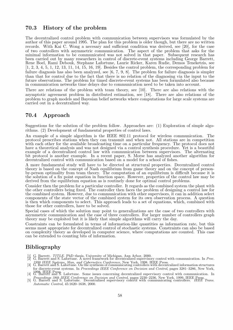
70.3 History of the problem

The decentralized control problem with communication between supervisors was formulated by theauthor of this paper around 1995. The plan for this problem is older though, but there are no writtenrecords. With Kai C. Wong a necesary and sufficient condition was derived, see [20], for the caseof two controllers with asymmetric communication. The aspect of the problem that asks for theminimal information to be communicated was not solved in that paper. Subsequent research hasbeen carried out by many researchers in control of discrete-event systems including George Barrett,Rene Boel, Rami Debouk, Stephane Lafortune, Laurie Ricker, Karen Rudie, Demos Teneketzis, see[1, 2, 3, 4, 5, 1, 12, 13, 11, 14, 15, 16, 19]. Besides the control problem, the corresponding problem forfailure diagnosis has also been analyzed, see [6, 7, 9, 8]. The problem for failure diagnosis is simplerthan that for control due to the fact that there is no relation of the diagnosing via the input to thefuture observations. The problem for timed discrete-event systems has been formulated also becausein communication networks time delays due to communication need to be taken into account.There are relations of the problem with team theory, see [10]. There are also relations with theasymptotic agreement problem in distributed estimation, see [18]. There are also relations of theproblem to graph models and Bayesian belief networks where computations for large scale systems arecarried out in a decentralized way.

70.4 Approach

Suggestions for the solution of the problem follow. Approaches are: (1) Exploration of simple algo-rithms. (2) Development of fundamental properties of control laws.An example of a simple algorithm is the IEEE 802.11 protocol for wireless communication. Theprotocol prescribes stations when they can transmit and when not. All stations are in competitionwith each other for the available broadcasting time on a particular frequency. The protocol does nothave a theoretical analysis and was not designed via a control synthesis procedure. Yet is a beautifulexample of a decentralized control law with communication between supervisors. The alternatingbit protocol is another example. In a recent paper, S. Morse has analyzed another algorithm fordecentralized control with communication based on a model for a school of fishes.A more fundamental study will have to be directed at structural properties. Decentralized controltheory is based on the concept of Nash equilibrium from game theory and on the concept of person-by-person optimality from team theory. The computation of an equilibrium is difficult because it isthe solution of a fix point equation in function space. However, properties of the control law may bederived from the equilibrium equation as is routinely done for optimal control problems.Consider then the problem for a particular controller. It regards as the combined system the plant withthe other controllers being fixed. The controller then faces the problem of designing a control law forthe combined system. However, due to communication with other supervisors, it can in addition selectcomponents of the state vector of the combined system for its own observation process. A questionis then which components to select. This approach leads to a set of equations, which, combined withthose for other controllers, have to be solved.Special cases of which the solution may point to generalizations are the case of two controllers withasymmetric communication and the case of three controllers. For larger number of controllers graphtheory may be exploited but it is likely that simple algorithms will carry the day.Constraints can be formulated in terms of information-like quantities as information rate, but thisseems most appropriate for decentralized control of stochastic systems. Constraints can also be basedon complexity theory as developed in computer science, where computations are counted. This casecan be extended to counting bits of information.

Bibliography

[1] G. Barrett. TITLE. PhD thesis, University of Michigan, Ann Arbor, 2000.[2] G. Barrett and S. Lafortune. A novel framework for decentralized supervisory control with communication. In Proc.

1998 IEEE Systems, Man, and Cybernetics Conference, New York, 1998. IEEE Press.[3] G. Barrett and S. Lafortune. On the synthesis of communicating controllers with decentralized information structures

for discrete-event systems. In Proceedings IEEE Conference on Decision and Control, pages 3281–3286, New York,1998. IEEE Press.

[4] G. Barrett and S. Lafortune. Some issues concerning decentralized supervisory control with communication. InProceedings 38th IEEE Conference on Decision and Control, pages 2230–2236, New York, 1999. IEEE Press.

[5] G. Barrett and S. Lafortune. Decentralized supervisory control with communicating controllers. IEEE Trans.Automatic Control, 45:1620–1638, 2000.

58

[6] R.K. Boel and Jan H. van Schuppen. Decentralized failure diagnosis for discrete-event systems with constrainedcommunication between diagnosers. In Proceedings Workshop on Discrete-Event Systems, 2002.

[7] R. Debouk. Failure diagnosis of decentralized discrete-event systems. PhD thesis, University of Michigan, AnnArbor, 2000.

[8] R. Debouk, S. Lafortune, and D. Teneketzis. Coordinated decentralized protocols for failure diagnosis of discrete-event systems. Discrete Event Dynamics Systems, 10:33–86, 2000.

[9] Rami Debouk, Stephane Lafortune, and Demosthesis Teneketzis. Coordinated decentralized protocols for failurediagnosis of discrete event systems. Report CGR-97-17, College of Engineering, University of Michcigan, Ann Arbor,1998.

[10] R. Radner. Allocation of a scarce resource under uncertainty: An example of a team. In C.B. McGuire andR. Radner, editors, Decision and organization, pages 217 – 236. North-Holland, Amsterdam, 1972.

[11] S. Ricker and K. Rudie. Know means no: Incorporating knowledge into decentralized discrete-event control. InProc. 1997 American Control Conference, 1997.

[12] S.L. Ricker. Knowledge and Communication in Decentralized Discrete-Event Control. PhD thesis, Queen’s Univer-sity, Department of Computing and Information Science, August 1999.

[13] S.L. Ricker and G. Barrett. Decentralized supervisory control with single-bit communications. In Proceedings ofAmerican Control Conference (ACC01), pages 965–966, 2001.

[14] S.L. Ricker and K. Rudie. Incorporating communication and knowledge into decentralized discrete-event systems.In Proceedings 38th IEEE Conference on Decision and Control, pages 1326–1332, New York, 1999. IEEE Press.

[15] S.L. Ricker and J.H. van Schuppen. Asynchronous communication in timed discrete event systems. In Proceedingsof the American Control Conference (ACC2001), pages 305–306, 2001.

[16] S.L. Ricker and J.H. van Schuppen. Decentralized failure diagnosis with asynchronuous communication betweensupervisors. In Proceedings of the European Control Conference (ECC2001), pages 1002–1006, 2001.

[17] S.C. Tatikonda. Control under communication constraints. PhD thesis, Department of Electrical Engineering andComputer Science, MIT, Cambridge, MA, 2000.

[18] D. Teneketzis and P. Varaiya. Consensus in distributed estimation with inconsistent beliefs. Systems & ControlLett., 4:217–221., 1984.

[19] J.H. van Schuppen. Decentralized supervisory control with information structures. In Proceedings InternationalWorkshop on Discrete Event Systems (WODES98), pages 36–41, London, 1998. IEE.

[20] K.C. Wong and J.H. van Schuppen. Decentralized supervisory control of discrete-event systems with communication.In Proceedings International Workshop on Discrete Event Systems 1996 (WODES96), pages 284–289, London, 1996.IEE.

59

Problem 80

Some control problems inelectromagnetics and fluid dynamics

Lorella FatoneDipartimento di Matematica Pura ed ApplicataUniversita di Modena e Reggio EmiliaVia Campi 213/b, 41100 Modena (MO), Italyfatone.lorella@unimo.it

Maria Cristina RecchioniIstituto di Teoria delle Decisioni e Finanza Innovativa (DE.F.IN.)Universita di AnconaPiazza Martelli 8, 60121 Ancona (AN), Italyrecchioni@posta.econ.unian.it

Francesco ZirilliDipartimento di Matematica “G. Castelnuovo”Universita di Roma “La Sapienza”Piazzale Aldo Moro 2, 00185 Roma, Italyf.zirilli@caspur.it

80.1 Introduction

In recent years, as a consequence of the dramatic increases in computing power and of the continuingrefinement of the numerical algorithms available, it has become possible the numerical treatment ofcontrol problems for systems governed by partial differential equations see, for example, [1], [3], [4], [5],[8]. The importance of these mathematical problems in many applications in science and technologycannot be overemphasized.The most common approach to a control problem for a system governed by partial differential equa-tions is to see the problem as a constrained nonlinear optimization problem in infinite dimension. Afterdiscretization the problem becomes a finite dimensional constrained nonlinear optimization problemthat can be attacked with the usual iterative methods of nonlinear optimization, such as Newton orquasi-Newton methods. Note that the problem of the convergence, when the “discretization step goesto zero”, of the solutions computed in finite dimension to the solution of the infinite dimensionalproblem is a separate question and must be solved separately. When this approach is used an objec-tive function evaluation in the nonlinear optimization procedure involves the solution of the partialdifferential equations that govern the system. Moreover the evaluation of the gradient or Hessianof the objective function involves the solution of some kind of sensitivity equations for the partialdifferential equations considered. That is the nonlinear optimization procedure that usually involvesfunction, gradient and Hessian evaluation is computationally very expensive. This fact is a seriouslimitation to the use of control problems for systems governed by partial differential equations in realsituations. However the approach previously described is very straightforward and does not use thespecial features present in each system governed by partial differential equations. So that, at least insome special cases, should be possible to improve on it.The purpose of this paper is to point out a problem, see [6], [2], where a new approach, that greatly

60

improves on the previously described one, has been introduced and to suggest some other problemswhere, hopefully, similar improvements can be obtained. In section 80.2 we summarize the resultsobtained in [6], [2], and in section 80.3 we present two problems that we belive can be approached ina way similar to the one described in [6], [2].

80.2 Previous results

In [6], [2] a furtivity problem in time dependent acoustic obstacle scattering is considered. An obstacleof known acoustic impedance is hit by a known incident acoustic field. When hit by the incidentacoustic field the obstacle generates a scattered acoustic field. To make the obstacle furtive meansto “minimize” the scattered field. The furtivity effect is obtained circulating on the boundary of theobstacle a “pressure current” that is a quantity whose physical dimension is: pressure divided by time.The problem consists in finding the optimal “pressure current” that “minimizes” the scattered field andthe “size” of the pressure current employed. The mathematical model used to study this problem is acontrol problem for the wave equation, where the control function (i.e. the pressure current) influencesthe state variable (i.e. the scattered field) through a boundary condition imposed on the boundary ofthe obstacle, and the cost functional depends explicitly from both the state variable and the controlfunction. Introducing an auxiliary variable and using the Pontryagin maximum principle (see [7]) in[6], [2] it is shown that the optimal control of this problem can be obtained from the solution of a systemof two coupled wave equations. This system of wave equations is equipped with suitable initial, finaland boundary conditions. Thanks to this ingenious construction the solution of the optimal controlproblem can be obtained solving the system of wave equations without the necessity of going throughthe iterations implied in general by the nonlinear optimization procedure. This fact avoids many ofthe difficulties, that have been mentioned above, present in the general case. Finally the system ofwave equations is solved numerically using a highly parallelizable algorithm based on the operatorexpansion method (for more details see [6], [2] and the references therein). Some numerical resultsobtained with this algorithm on simple test problems can be seen in the form of computer animationsin the websites: http://www.econ.unian.it/recchioni/w6, http://www.econ.unian.it/recchioni/w8. In thefollowing section we suggest two problems where will be interesting to carry out a similar analysis.

80.3 Two control problems

Let R be the set of real numbers, x = (x1, x2, x3)T ∈ R3 (where the superscript T means transposed)be a generic vector of the three-dimensional real Euclidean space R3, and let (·, ·), ‖ ·‖ and [·, ·] denotethe Euclidean scalar product, the Euclidean vector norm and the vector product in R3 respectively.The first problem suggested is a “masking” problem in time dependent electromagnetic scattering.Let Ω ⊂ R3 be a bounded simply connected open set (i.e. the obstacle) with locally Lipschitzboundary ∂Ω. Let Ω denote the closure of Ω and n(x) = (n1(x), n2(x), n3(x))T ∈ R3, x ∈ ∂Ω bethe outward unit normal vector in x for x ∈ ∂Ω. Note that n(x) exists almost everywhere in x forx ∈ ∂Ω. We assume that the obstacle Ω is characterized by an electromagnetic boundary impedanceχ > 0. Note that χ = 0 (χ = +∞) corresponds to consider a perfectly conducting (insulating)obstacle. Let R3 \ Ω be filled with a homogeneous isotropic medium characterized by a constantelectric permittivity ε > 0, a constant magnetic permeability ν > 0, zero electric conductivity, zerofree charge density and zero free current density. Let (Ei(x, t),Bi(x, t)), (x, t) ∈ R3 × R (whereEi is the electric field and Bi is the magnetic induction field) be the incoming electomagnetic fieldpropagating in the medium filling R3\Ω and satisfying the Maxwell equations (80.1)-(80.3) in R3×R.Let (Es(x, t),Bs(x, t)), (x, t) ∈ (R3 \Ω)×R be the electromagnetic field scattered by the obstacle Ωwhen hit by the incoming field (Ei(x, t),Bi(x, t)), (x, t) ∈ R3×R. The scattered electric field Es andthe scattered magnetic induction field Bs satisfy the following equations:(

curlEs +∂Bs

∂t

)(x, t) = 0, (x, t) ∈ (R3 \ Ω)×R, (80.1)

(curlBs − 1

c2

∂Es

∂t

)(x, t) = 0, (x, t) ∈ (R3 \ Ω)×R, (80.2)

61

divBs(x, t) = 0, divEs(x, t) = 0, (x, t) ∈ (R3 \ Ω)×R, (80.3)

[n(x),Es(x, t)]− cχ[n(x), [n(x),Bs(x, t)]] =−[n(x),Ei(x, t)] + cχ[n(x), [n(x),Bi(x, t)]], (x, t) ∈ ∂Ω×R, (80.4)

Es(x, t) = O

(1r

), [Bs(x, t), x]− 1

cEs(x, t) = o

(1r

), r → +∞, t ∈ R, (80.5)

where 0 = (0, 0, 0)T , c = 1/√ε ν, r = ‖x‖, x ∈ R3, x = x

‖x‖ , x 6= 0,x ∈ R3, O(·) and o(·) are theLandau symbols, and curl· and div· denote the curl and the divergence operator of · with respect tothe x variables respectively.A classical problem in electromagnetics consists in the recognition of the obstacle Ω through theknowledge of the incoming electromagnetic field and of the scattered field (Es(x, t),Bs(x, t)), (x, t) ∈(R3 \ Ω) × R solution of (80.1)-(80.5). In the above situation Ω plays a “passive” (“static”) role.We want to make the obstacle Ω “active” (“dynamic”) in the sense that, thanks to a suitable controlfunction chosen in a proper way, the obstacle itself tries to react to the incoming electromagnetic fieldproducing a scattered field that looks like the field scattered by a preassigned obstacle D (the“mask”)with impedance χ′. More in details we suggest to consider the following control problem:Problem 1 Electromagnetic “Masking” Problem: Given an incoming electromagnetic field (Ei,Bi),an obstacle Ω and its electromagnetic boundary impedance χ, and given an obstacle D such thatD ⊂ Ω with electromagnetic boundary impedance χ′, choose a vector control function ψ defined onthe boundary of the obstacle ∂Ω for t ∈ R and appearing in the boundary condition satisfied bythe scattered electromagnetic field on ∂Ω, in order to minimize a cost functional that measures the“difference” between the electromagnetic field scattered by Ω, i.e. (Es,Bs), and the electromagneticfield scattered by D, i.e. (EsD,B

sD), when Ω and D respectively are hit by the incoming field (Ei,Bi),

and the “size” of the vector control function employed.The control function ψ has the physical dimension of an electric field and the action of the optimalcontrol electric field on the boundary of the obstacle makes the obstacle “active” (“dynamic”) andable to react to the incident electromagnetic field to become “unrecognizable”, that is “Ω will do itsbest to appear as his mask D”.The second control problem we suggest to consider is a control problem in fluid dynamics. Let usconsider an obstacle Ωt, t ∈ R, that is a rigid body, assumed homogeneous, moving in R3 with velocityυ = υ(x, t), (x, t) ∈ Ωt×R. Moreover for t ∈ R the obstacle Ωt ⊂ R3 is a bounded simply connectedopen set. For t ∈ R let ξ = ξ(t) be the position of the center of mass of the obstacle Ωt. The motionof the obstacle is completely described by the velocity w = w(ξ, t), t ∈ R of the center of mass of

the obstacle (i.e. w =dξ

dt, t ∈ R), the angular velocity ω = ω(ξ, t), t ∈ R of the obstacle around the

instantaneous rotation axis going through the center of mass ξ = ξ(t), t ∈ R and the necessary initialconditions. Note that the velocities of the points belonging to the obstacle υ(x, t), (x, t) ∈ Ωt × Rcan be expressed in terms of w(ξ, t),ω(ξ, t), t ∈ R. Let R3 \ Ωt, t ∈ R be filled with a Newtonianincompressible viscous fluid of viscosity η. We assume that both the density of the fluid and thetemperature are constant. For example Ωt, t ∈ R can be a submarine or an airfoil immersed in anincompressible viscous fluid. Let v = (v1, v2, v3)T and p be the velocity field and the pressure field ofthe fluid respectively, f be the density of the external forces per mass unit acting on the fluid, andv−∞ be an assigned solenoidal vector field. We assume that in the limit t → −∞ the body Ωt isat rest in the position Ω−∞. Under these assumptions we have that in the reference frame given byx = (x1, x2, x3)T the following system of Navier-Stokes equations holds:

∂v

∂t(x, t) + (v(x, t),∇)v(x, t)− η∆v(x, t) +∇p(x, t) = f(x, t),

(x, t) ∈ (R3 \ Ωt)×R ,(80.6)

div v(x, t) = 0, (x, t) ∈ (R3 \ Ωt)×R , (80.7)

limt→−∞

v(x, t) = v−∞(x), x ∈ R3 \ Ω−∞ ,v(x, t) = υ(x, t), (x, t) ∈ ∂Ωt ×R. (80.8)

62

In (80.6) we have ∇ =(

∂∂x1

, ∂∂x2

, ∂∂x3

)Tand (v,∇)v =

(∑3j=1 vj

∂v1∂xj

,∑3

j=1 vj∂v2∂xj

,∑3

j=1 vj∂v3∂xj

)T.

The boundary condition in (80.8) requires that the fluid velocity v and the velocity of the obstacleυ are equal on the boundary of the obstacle for t ∈ R. We want to consider the problem associatedto the choice of a manoeuvre w(ξ, t), ω(ξ, t), t ∈ R connecting two given states that minimizes thework done by the obstacle Ωt, t ∈ R against the fluid going from the initial state to the final state,and the “size” of the manoeuvre employed. Note that in this context a manoeuvre connecting twogiven states is made of two functions w(ξ, t),ω(ξ, t), t ∈ R such that limt→±∞w(ξ, t) = w± andlimt→±∞ω(ξ, t) = ω±, where w± and ω± are preassigned. The couple (w−,ω−) is the initial stateand the couple (w+,ω+) is the final state. For simplicity we have assumed (w−,ω−) = (0,0). Weformulate the following problem:Problem 2 “Drag” Optimization Problem: Given a rigid obstacle Ωt, t ∈ R moving in a Newtonianfluid characterized by a viscosity η and the initial condition and forces acting on the fluid, and giventhe initial state (0,0) and the final state (w+,ω+), choose a manoeuvre connecting these two statesin order to minimize a cost functional that measures the work that the obstacle Ωt, t ∈ R must exerton the fluid to make the manoeuvre, and the “size” of the manoeuvre employed.From the previous considerations several problems arise. The first one is connected with the questionof formulating Problem 1 and Problem 2 as control problems. In [2] we suggest a possible formulationof a furtivity problem similar to Problem 1 as a control problem. Many variations of Problem 1 and2 can be considered. For example in Problem 1 we have assumed, for simplicity, that the “mask”is a passive obstacle, that is (EsD(x, t),Bs

D(x, t)), (x, t) ∈ (R3 \ D) × R is the solution of problem(80.1)-(80.5) when Ω, χ are replaced with D,χ′ respectively. In a more general situation also the“mask” can be an active obstacle. Finally Problem 1 and 2 are examples of control problems forsystems governed by the Maxwell equations and the Navier-Stokes equations respectively. Many otherexamples involving different partial differential equations can be considered.

Bibliography

[1] T. S. Angell, A. Kirsch and R. E. Kleinman, “Antenna control and optimization”, Proceedings ofthe IEEE, 79, pp. 1559-1568 (1991).

[2] L. Fatone, M. C. Recchioni and F. Zirilli, “Furtivity and masking problems in time dependentacoustic obstacle scattering”, submitted to Third ISAAC Congress Proceedings (2002).

[3] J. W. He, R. Glowinski, R. Metcalfe, A. Nordlander and J. Periaux, “Active control and DragOptimization for Flow Past a Circular Cylinder”, Journal of Computational Physics, 163, pp.83-117 (2000).

[4] J. E. Lagnese, “A singular perturbation problem in exact controllability of the Maxwell system”,ESAIM Control, Optimization and Calculus of Variations, 6, pp. 275-289 (2001).

[5] J. Luniley and P. Blossery, “Control of turbulence”, Annual Review of Fluid Mechanics, 30, pp.311-327 (1998).

[6] F. Mariani, M.C. Recchioni and F. Zirilli, “The use of the Pontryagin maximum principle in afurtivity problem in time-dependent acoustic obstacle scattering”, Waves in Random Media, 11,pp. 549-575 (2001).

[7] L. Pontriaguine, V. Boltianski, R. Gamkrelidze and F. Micktckenko, “Theorie Mathematique desProcessus Optimaux”, Editions Mir, Moscou (1974).

[8] S. S. Sritharan, “An introduction to deterministic and stochastic control of viscous flow”, in Op-timal Control of Viscous Flow, S. S. Sritharan Editor, SIAM, Philadelphia, pp. 1-42 (1998).

63

Problem 19

A conjecture on Lyapunov equationsand principal angles in subspaceidentification

Katrien De Cock and Bart De Moor1

Dept. of Electrical Engineering (ESAT–SCD)K.U.LeuvenKasteelpark Arenberg 10B-3001 LeuvenBelgiumTel. 32/16/32 17 09, Fax 32/16/32 19 70http://www.esat.kuleuven.ac.be/sista-cosic-docarchdecock@esat.kuleuven.ac.be, demoor@esat.kuleuven.ac.be

19.1 Description of the problem

The following conjecture relates the eigenvalues of certain matrices that are derived from the solution ofa Lyapunov equation that occurred in the analysis of stochastic subspace identification algorithms [3].First, we formulate the conjecture as a pure matrix algebraic problem. In Section 19.2, we will describeits system theoretic consequences and interpretation.

Conjecture 2 Let A ∈ Rn×n be a real matrix and v, w ∈ Rn be real vectors so that there are no twoeigenvalues λi and λj of

(A 00 A+ vwT

)for which λiλj = 1 (i, j = 1, . . . , 2n). If the n× n matrices

P , Q and R satisfy the Lyapunov equation

(P RRT Q

)=(A 00(A+ vwT

)T)( P RRT Q

)(AT 00 A+ vwT

)+(vw

)(vT wT ) , (19.1)

and P , Q and (In + PQ) are non-singular2, then the matrices P−1RQ−1RT and (In + PQ)−1 havethe same eigenvalues.

1Katrien De Cock is a research assistant at the K.U.Leuven. Dr. Bart De Moor is a full professor at the K.U.Leuven.Our research is supported by grants from several funding agencies and sources: Research Council KUL: Concerted Re-search Action GOA-Mefisto 666, IDO, several PhD, postdoc & fellow grants; Flemish Government: Fund for ScientificResearch Flanders (several PhD and postdoc grants, projects G.0256.97, G.0115.01, G.0240.99, G.0197.02, G.0407.02, re-search communities ICCoS, ANMMM), AWI (Bil. Int. Collaboration Hungary/ Poland), IWT (Soft4s, STWW-Genprom,GBOU-McKnow, Eureka-Impact, Eureka-FLiTE, several PhD grants); Belgian Federal Government: DWTC (IUAP IV-02 (1996-2001) and IUAP V-22 (2002-2006)), Program Sustainable Development PODO-II (CP/40); Direct contractresearch: Verhaert, Electrabel, Elia, Data4s, IPCOS.

2The matrix In is the n× n identity matrix.

64

Note that the condition λiλj 6= 1 (∀i, j = 1, . . . , 2n) ensures that there exists a solution(P RRT Q

)of

the Lyapunov equation (19.1) and that the solution is unique.We have checked the similarity of P−1RQ−1RT and (In + PQ)−1 for numerous examples (“proof byMatlab”) and it is simple to prove the conjecture for n = 1. Furthermore, via a large detour (see [3]) wecan also prove it from the system theoretic interpretation, which is given in Section 19.2.3. However,we have not been able to find a general and elegant proof.We also remark that the requirement that v and w are vectors, is necessary for the conjecture to hold.One can easily find counterexamples for the case V,W ∈ Rn×m, where m > 1. It is consequently clearthat this condition on v and w should be used in the proof.

19.2 Background and motivation

Although the conjecture is formulated as a pure matrix algebraic problem, its system theoretic inter-pretation is particularly interesting. In order to explain the consequences, we first have to introducesome concepts: the principal angles between subspaces (Section 19.2.1) and their statistical counter-parts, the canonical correlations of random variables (Section 19.2.2). Next, in Section 19.2.3 we willshow how the conjecture – when proved correct – would enable us to prove in an elegant way that thenon-zero canonical correlations of the past and the future of the output process of a linear stochasticmodel are equal to the sines of the principal angles between two specific subspaces that are derivedfrom the model. This result, in its turn, is instrumental for further derivations in [3], where a cepstraldistance measure is related to canonical correlations and to the mutual information of two processes(see also Section 19.2.3). Moreover, by this new characterization of the canonical correlations we gaininsight in the geometric properties of subspace based techniques.

19.2.1 The principal angles between two subspaces

The concept of principal angles between and principal directions in subspaces of a linear vector spaceis due to Jordan in the nineteenth century [8]. We give the definition and briefly describe how theprincipal angles can be computed.Let S1 and S2 be subspaces of Rn of dimension p and q respectively, where p ≤ q. Then, the p principalangles between S1 and S2, denoted by θ1, . . . , θp, and the corresponding principal directions ui ∈ S1

and vi ∈ S2 (i = 1, . . . , p) are recursively defined as

cos θ1 = maxu∈S1

maxv∈S2

|uT v| = uT1 v1

cos θk = maxu∈S1

maxv∈S2

|uT v| = uTk vk (k = 2, . . . , p)

subject to ‖u‖ = ‖v‖ = 1, and for k > 1: uTui = 0 and vT vi = 0, where i = 1, . . . , k − 1.If S1 and S2 are the row spaces of the matrices A ∈ Rl×n and B ∈ Rm×n respectively, then thecosines of the principal angles θ1, . . . , θp, can be computed as the largest p generalized eigenvalues ofthe matrix pencil (

0 ABT

BAT 0

)−(AAT 0

0 BBT

)λ .

Furthermore, if A and B are full row rank matrices, i.e. l = p and m = q, then the squared cosines ofthe principal angles between the row space of A and the row space of B are equal to the eigenvaluesof

(AAT )−1ABT (BBT )−1BAT .

Numerically stable methods to compute the principal angles via the QR and singular value decompo-sition can be found in [5, pp. 603–604].

19.2.2 The canonical correlations of two random variables

Canonical correlation analysis, due to Hotelling [6], is the statistical version of the notion of principalangles.

65

Let X ∈ Rp and Y ∈ Rq, where p ≤ q, be zero-mean random variables with full rank joint covariancematrix3

Q = E(XY

)(XT Y T )

=(Qx QxyQyx Qy

).

The canonical correlations ofX and Y are defined as the largest p eigenvalues of the pencil( 0 QxyQyx 0

)−(

Qx 00 Qy

)λ. More information on canonical correlation analysis can be found in [1, 6].

19.2.3 System theoretic interpretation of Conjecture 2

Let y(k)k∈Z be a real, discrete-time, scalar and zero-mean stationary stochastic process that isgenerated by the following single-input single-output (SISO), asymptotically stable state space modelin forward innovation form:

x(k + 1) = Ax(k) +Ku(k) ,y(k) = Cx(k) + u(k) , (19.2)

where u(k)k∈Z is the innovation process of y(k)k∈Z, A ∈ Rn×n, K ∈ Rn×1 is the Kalman gain andC ∈ R1×n. The state space matrices of the inverse model (or whitening filter) are A − KC, K and−C respectively, as is easily seen by writing u(k) as an output with y(k) as an input.By substituting the vector v in (19.1) by K, and w by −CT , the matrices P , Q and R in (19.1) canbe given the following interpretation. The matrix P is the controllability Gramian of the model (19.2)and Q is the observability Gramian of the inverse model, while R is the cross product of the infinitecontrollability matrix of (19.2) and the infinite observability matrix of the inverse model. Otherwiseformulated: (

P RRT Q

)=(

C∞ΓT∞

)(CT∞ Γ∞) ,

where C∞ = (K AK A2K · · ·) and Γ∞ = −

C

C(A−KC)C(A−KC)2

...

.

Due to the stability and the minimum phase property of the forward innovation model (19.2), theseinfinite products result in finite matrices and in addition, the condition λiλj 6= 1 in Conjecture 2 isfulfilled. Furthermore, under fairly general conditions, P , Q and In + PQ are non-singular, whichfollows from the positive definiteness of P and Q under general conditions.The matrix P−1RQ−1RT in Conjecture 2 is now equal to the product

(C∞CT∞)−1(C∞Γ∞)(ΓT∞Γ∞)−1(ΓT∞CT∞) .

Consequently, its n eigenvalues are the squared cosines of the principal angles between the row spaceof C∞ and the column space of Γ∞ (see Section 19.2.1). The angles will be denoted by θ1, . . . , θn (innon-decreasing order).The eigenvalues of the matrix (In+PQ)−1, on the other hand, are related to the canonical correlationsof the past and the future stochastic processes of y(k)k∈Z, which are defined as the canonicalcorrelations of the random variables

yp =

y(−1)y(−2)y(−3)

...

and yf =

y(0)y(1)y(2)

...

,

and denoted by ρ1, ρ2, . . . (in non-increasing order). It can be shown [3] that the largest n canonicalcorrelations of yp and yf are equal to the square roots of the eigenvalues of In − (In + PQ)−1. Theother canonical correlations are equal to 0.

3E · is the expected value operator.

66

Conjecture 2 now gives us the following characterization of the canonical correlations of the past andthe future of y(k)k∈Z: the largest n canonical correlations are equal to the sines of the principalangles between the row space of C∞ and the column space of Γ∞ and the other canonical correlationsare equal to 0:

ρ1 = sin θn, ρ2 = sin θn−1, . . . , ρn = sin θ1, ρn+1 = ρn+2 = · · · = 0 . (19.3)

This result can be used to prove that a recently defined cepstral norm [9] for a model as in (19.2) isclosely related to the mutual information of the past and the future of its output process. Let thetransfer function of the system in (19.2) be denoted by H(z). Then, the complex cepstrum c(k)k∈Zof the model is defined as the inverse Z-transform of the complex logarithm of H(z):

c(k) =1

2πi

∮C

log(H(z))zk−1 dz ,

where the complex logarithm of H(z) is appropriately defined (see [10, pp. 495–497]) and the contourC is the unit circle. The cepstral norm that we consider, is defined as

‖ logH‖2 =∞∑k=0

kc(k)2 .

As we have proven in [2], it can be characterized in terms of the principal angles θ1, . . . , θn betweenthe row space of C∞ and the column space of Γ∞ as follows:

‖ logH‖2 = − logn∏i=1

cos2 θi ,

and from (19.3) we obtain‖ logH‖2 = − log

∏(1− ρ2

i ) .

The relation∑∞

k=0 kc(k)2 = − log∏

(1 − ρ2i ) was also reported in [7, Proposition 2]. Moreover, if

y(k)k∈Z is a Gaussian process, then the expression −12 log

∏(1 − ρ2

i ) is equal to the mutual infor-mation of its past and future (see e.g. [4]), which is denoted by I(yp; yf ). Consequently,

‖ logH‖2 =∞∑k=0

kc(k)2 = 2I(yp; yf ) .

19.3 Conclusions

We presented a matrix algebraic conjecture on the eigenvalues of matrices that are derived from thesolution of a Lyapunov equation. We showed that a proof of Conjecture 2 would provide yet anotherelegant geometric result in the subspace based study of linear stochastic systems. Moreover, it can beused to express a cepstral distance measure that was defined in [9] in terms of canonical correlationsand also as the mutual information of two processes.

Bibliography

[1] T. W. Anderson, An Introduction to Multivariate Statistical Analysis, John Wiley & Sons, NewYork (1984).

[2] K. De Cock and B. De Moor, “Subspace Angles Between ARMA Models”, Technical Report4 00-44a, ESAT-SCD, K.U.Leuven (Leuven, Belgium), accepted for publication in Systems & ControlLetters (2002).

4This report is available by anonymous ftp from ftp.esat.kuleuven.ac.be in the directory pub/sista/reports as file00-44a.ps.gz.

67

[3] K. De Cock, “Principal Angles in System Theory, Information Theory and Signal Processing”,PhD thesis5, Faculty of Applied Sciences, K.U.Leuven (Leuven, Belgium) (2002).

[4] I. M. Gel’fand and A. M. Yaglom, “Calculation of the Amount of Information About a RandomFunction Contained in Another Such Function”, American Mathematical Society Translations,Series (2), 12, pp. 199–236 (1959).

[5] G. H. Golub and C. F. Van Loan, Matrix Computations, The Johns Hopkins University Press,Baltimore (1996).

[6] H. Hotelling, “Relations Between Two Sets of Variates”, Biometrika, 28, pp. 321–372 (1936).[7] N. P. Jewell, P. Bloomfield, and F. C. Bartmann, “Canonical Correlations of Past and Future for

Time Series: Bounds and Computation”, The Annals of Statistics, 11, pp. 848–855 (1983).[8] C. Jordan, “Essai sur la geometrie a n dimensions”, Bulletin de la Societe Mathematique, 3,

pp. 103–174 (1875).[9] R. J. Martin, “A Metric for ARMA Processes”, IEEE Transactions on Signal Processing, 48,

pp. 1164–1170 (2000).[10] A. V. Oppenheim and R. W. Schafer, Digital Signal Processing, Prentice/Hall International

(1975).

5This thesis will also be made available by anonymous ftp from ftp.esat.kuleuven.ac.be as filepub/sista/decock/reports/phd.ps.gz

68

Problem 84

On the Computational Complexity ofNon-Linear Projections and itsRelevance to Signal Processing

Jonathan H. MantonDepartment of Electrical and Electronic EngineeringThe University of Melbourne, Victoria 3010, Australiajon@ee.mu.oz.au

Robert MahonyDepartment of EngineeringAustralian National University, ACT 0200, Australiamahony@ieee.org

84.1 Description of the Problem

Recent advances in finding the roots of a non-linear equation to within a specified level of accuracyhas lead to a novel approach to studying computational complexity of real valued problems [1]. Thischapter considers a similar problem, that of globally solving non-linear projection problems to within aspecified level of accuracy. A host of important problems derived from signal processing and telecom-munications engineering may be written in this form. Optimal solutions are usually intractable andit is important to understand the computational complexity of solving such problems approximatelyin order that effective sub-optimal algorithms may be developed.Consider a non-linear (non-convex) minimisation problem of the form

arg minx∈Rn

‖y − f(x)‖2 (84.1)

for a given y ∈ Rm and function f : Rn → Rm. Although (84.1) has several interpretations, including

a least-squares interpretation and a non-linear regression interpretation, the interpretation favouredhere is that if x minimises (84.1) then f(x) is the point in the image of f closest to y. Indeed, (84.1)is solved conceptually by first projecting y onto the set

Y = y ∈ Rm : y = f(x), x ∈ Rn (84.2)

and then computing the pre-image. Sometimes only the projection f(x) and not the pre-image x isof interest, while other times, only certain elements of x are of interest. This motivates studying themore general problem:

Calculate g(x) where x = arg minx∈Rn

‖y − f(x)‖2 (84.3)

for some function g : Rn → Rp. Clearly, if g is taken to be g(x) = f(x) then (84.3) is precisely the

projection of y onto the image of f .

69

The practical goal of an engineer in solving a problem of the form (84.3) is to develop a tractablenumerical algorithm that, for any input y, outputs an approximate solution that is sufficiently accuratefor the application considered. Inherent in the formulation is the trade-off between computationalcomplexity and accuracy; the more accurate the solution is required to be, the harder it is to obtain.To evaluate a potential algorithm one wishes to compare its complexity with the intrinsic complexityof the problem (84.3). The following two definitions provide a framework in which this comparisonmay be made. The definitions here are motivated by those proposed recently by Smale et al. [1].

Definition 1 (ε-accurate solution) For a given ε > 0, an ε-accurate solution of (84.3) is a vectors ∈ Rp satisfying the condition

‖s− g(x)‖ < ε, x = arg minx∈Rn

‖y − f(x)‖2. (84.4)

(In the event that ‖y−f(x)‖2 does not have a unique minimum, an ε-accurate solution is one satisfying(84.4) for some x in the set of all x minimising ‖y − f(x)‖2.)

Definition 2 (Computational complexity) Only algorithms of the following form are consideredfor solving (84.3). Let R be an integer and let ri : Rm → R for i = 1, · · · , 2R − 1 and hj : Rm → R

p

for j = 1, · · · , 2R be sequences of rational1 functions. The ri are used to divide the space y lies in into2R regions as follows. Initially, set i := 1. While i < 2R, evaluate ri(y) and set i := 2i if ri(y) < 0and set i := 2i + 1 otherwise. Finally, set j := i − 2R + 1. (This results in a j lying between 1 and2R.) Based on this region j, the algorithm outputs s := hj(y). Each of these operations involves acertain number of multiplications and additions; for simplicity, the complexity of evaluating a rationalfunction is taken to be the degree of its numerator plus the degree of its denominator. (The hj aretreated as comprising p rational functions from R

m to R.) For a given y, the complexity of the abovealgorithm is deduced by summing the complexity of the functions encountered. The overall complexityof the algorithm is defined to be the largest complexity over all possible y.Given a function f and an accuracy ε, the computational complexity of implementing the non-linearprojection operator (84.3) is said to be upper bounded by N(ε; f) if there exists an algorithm of theabove form with complexity at most N and which is guaranteed to find an ε-accurate solution of (84.3)for all y.

These definitions provide a formulation in which one may evaluate the relative difficulty of a numberof interesting problems.

Problem 1 Let g : Rn → Rp be a known function2. Consider three classes of function f

1. Let f : Rn → Rm be a bilinear function.

2. Let D be a positive integer. Let f : Rn → Rm be a generic polynomial of degree D.

3. Let ρ > 0 be a positive constant. Let f be a smooth function with ||D2f || < 1/ρ. That is thatthe curvature of the injective image f : Rn → R

m is locally bounded above by ρ.

For each of the given classes of functions f compute a bound on the complexity N(ε; f) (cf. Def. 2)for any function f in the class considered.

Of the three classes of functions proposed the first is strongly motivated by the joint filtering/systemidentification problem for a linear system. The second class of functions considered (generic polyno-mials) are chosen to link directly to the structure of Definition 2 and earlier work on the algebraiccomplexity of finding the roots of polynomials [2, 1, 3]. Finally, applying a condition on the curvatureof the image of f(x) should reduce the complexity of the local projection problem. The global com-plexity may still lead to an intractable problem in the general formulation, however, in practice this

1A rational function is a ratio of two polynomial functions.2The three typical choices for the function g are i) g(x) = x, ii) g(x) is a linear projection of x, and iii) g(x) = f(x).

70

difficulty may not be encountered when real engineering problems are considered (cf. Prob. 2). Theclasses of functions considered in Problem 1 are clearly a drop in the ocean of possibilities. An equallyimportant question would be to identify the key classes of functions f that relate closely to practicalengineering problems and lead to a tractable computational complexity analysis.Requiring the algorithm in Definition 2 to find an ε-accurate solution for all y is a strong globalcondition. In practical applications, extra knowledge about y is often available. An example is wheny = f(x)+n where n is a noise vector. If the noise variance is sufficiently small then y will generally lieclose to the image of f . Exploiting this fact may lead to significantly better performance of a filter [4].Indeed, most signal processing algorithms perform well when the noise variance is sufficiently small.This motivates the following problem:

Problem 2 Let g : Rn → Rp be a known function (cf. Prob. 1)). For a given δ > 0, define the set

Yδ = y ∈ Rm : ∃x ∈ Rn, ‖y − f(x)‖ ≤ δ . (84.5)

Define N(ε, δ; f) as in Definition 2 but with the weaker requirement that the algorithm find an ε-accurate solution for all y ∈ Yδ.Consider the three classes of functions f described in Problem 1 parts 1)-3). Compute a bound on thecomplexity N(ε, δ; f) for any function f in the class considered.

Remarks: i) A feature of Definition 2 is that it ignores round-off error. For example, according toDefinition 2, y = Ax can be inverted exactly in a finite number of operations. Although Definition 2can be modified to take round-off error into account, it is preferable to ignore round-off error and focusinstead on the inherent difficulty in computing algebraically a non-linear projection.ii) If f is a polynomial function then the closure of Y is a variety (i.e., an irreducible algebraic set) [3]and can thus be made into a manifold by removing a set of measure zero. Therefore, the essentialproblem considered here is the complexity of computing the projection of a point onto a manifold.

84.2 Motivation and History

The motivation for studying the complexity of non-linear projection operators is twofold; from a math-ematical perspective, it is a natural generalisation of Smale’s recent work [1]. From a signal processingperspective, because the main computational difficulty in many applications is that of computing anon-linear projection, understanding the intrinsic complexity of a non-linear projection operator is asignificant step towards understanding the intrinsic complexity of signal processing problems.

84.2.1 Intrinsic Complexity of Signal Processing Algorithms

Some signal processing problems have a reputation for being harder to solve than others. A funda-mental question then is whether or not this notion of difficulty can be made mathematically precise.Motivating examples of signal processing problems reducing to a problem of the form (84.3) are givenbelow. This shows their inherent complexity can be defined as in Section 1.The harmonic retrieval problem, in its simplest form, is to determine the frequency f of a noisecorrupted sinusoid yi = a cos(2πfi+ θ) +ni where ni is noise. Let x = (a, f, θ) be a three-dimensionalvector and define f : R3 → R

m component-wise by the rule fi(a, f, θ) = a cos(2πfi + θ). Defineg : R3 → R by g(a, f, θ) = f . Then the solution of (84.3) is the least-squares estimate of the frequencyf .An important class of problems of significant interest is the dual identification and and filtering problemfor any system. Let x = (θ, s) where θ parameterises a class of systems functions fθ and s denotes theinput sequence. The minimization problem

s = arg mins

infθ‖y − fθ(s)‖2

,

solves for an estimate of the input signal based on minimizing a least squares cost in the observationspace. If the system class fθ is linearly parameterised and consists of linear systems then f(θ, s) :=fθ(s) is a bilinear function. This formulation leads directly to Problem 1-1).

71

84.2.2 Real Complexity Theory

Rigorously defining the complexity of an engineering problem is challenging. Traditional computationalcomplexity theory, which studies the number of operations a Turing machine requires to solve aparticular problem, is not suitable. Indeed, a Turing machine cannot process real valued numbers asit has no way of storing or manipulating irrational numbers in general.In a series of recent papers (see [1] for references), Steve Smale and his coworkers proposed an alterna-tive definition of computational complexity which can handle problems involving real valued numbers.Central to Smale’s work is a measure of how computationally complicated it is to find all the rootsof the equation f(x) = 0 to within an accuracy ε. Also of interest is the fact that, for a given f andaccuracy ε, Smale proposed a homotopy-like iterative algorithm which is guaranteed to find all theroots of f to within ε, and moreover, requires at most N iterations to do so, where N depends on fand on ε; see [1] for details.Although a root finding algorithm can be used to solve (84.1), determining the complexity of (84.1) isa more general problem than determining the complexity of root finding. For a given y, define g(x; y)to be the derivative of ‖y − f(x)‖2. Then (84.1) can be solved by finding all the roots of g(x; y) = 0and determining which roots globally minimise ‖y−f(x)‖2. However, it has not been established thatroot finding is the best way of solving (84.1) or (84.3); that is, the intrinsic computational complexityof (84.1) conceivably may be considerably lower than the computational complexity of the associatedroot finding problem.Therefore, determining the complexity of non-linear projections is an extension of the complexityresults for root finding in [1].

84.3 Available Results

Real computational complexity theory, as opposed to traditional computational complexity theory,is a new subject [1]. Nevertheless, some advanced results appear in [1] which can be applied to thenon-linear projection problem. For instance, the homotopy-like method in [1] for finding all the rootsof g(x) = 0 can be used to solve (84.1) for a given y by setting g(x) to the derivative of ‖y − f(x)‖2.It is likely though that better techniques exist, and it is hoped this article will stimulate research inthis area.

Acknowledgments: The authors would like to thank Gunnar Ratsch for a number of interesting anduseful discussions.

Bibliography

[1] L. Blum, F. Cucker, M. Shub, and S. Smale. Complexity and Real Computation. Springer, 1997.[2] D. A. Cox, J. B. Little, and D. O’Shea. Using Algebraic Geometry. Springer-Verlag, 1998.[3] R. Hartshorne. Algebraic Geometry. Springer-Verlag, 1977.[4] J. H. Manton and B.-N. Vo. Fisher information decision directed quantisation: A fast sub-optimal

solution to discrete optimisation problems with applications in wireless communications. In In-ternational Conference on Optimisation Theory and Applications, volume 1, pages 316–323, HongKong, December 2001.

72

Problem 2

H∞-norm approximation

A.C. AntoulasDepartment of Electrical and Computer EngineeringRice University6100 South Main StreetHouston, Texas 77005-1892USAaca@rice.edu

A. AstolfiDepartment of Electrical and Electronic EngineeringImperial CollegeExhibition RoadSW7 2BT, LondonUnited Kingdoma.astolfi@ic.ac.uk

2.1 Description of the problem

Let RHm∞ be the (Hardy) space of real-rational scalar1 transfer functions of order m, bounded on the

imaginary axis and analytic into the right-half complex plane. The optimal approximation problemin the H∞ norm can be stated as follows.

(A?) (Optimal Approximation in the H∞ norm)Given G(s) ∈ RHN

∞ and an integer n < N find2 A?(s) ∈ RHn∞ such that

A?(s) = arg minA(s)∈RHn∞‖G(s)−A(s)‖∞. (2.1)

For such a problem, letγ?n = minA(s)∈RHn

∞‖G(s)−A(s)‖∞,

then two further problems can be posed.

(D) (Optimal Distance problem in the H∞ norm)Given G(s) ∈ RHN

∞ and an integer n < N find γ?n.

(A) (Sub-optimal Approximation in the H∞ norm)Given G(s) ∈ RHN

∞, an integer n < N and γ > γ?n find A(s) ∈ RHn∞ such that

γ?n ≤ ‖G(s)− A(s)‖∞ ≤ γ.1Similar considerations can be done for the non-scalar case.2By find we mean find an exact solution or an algorithm converging to the exact solution.

73

The optimal H∞ approximation problem can be formally posed as a constrained min-max problem.For, note that any function in RHn

∞ can be put in a one to one correspondence with a point θ of some(open) set Ω ⊂ R2n, therefore the problem of computing γ?n can be posed as

γ?n = minθ∈Ω

maxω∈R‖G(jω)−A(jω)‖, (2.2)

where A(s) = A(s, θ). The above formulation provides a brute force approach to the solution of theproblem. Unfortunately, this method is not of any use in general, because of the complexity of the setΩ and because of the curse of dimensionality. However, the formulation (2.2) suggests that possiblecandidate solutions of the optimal approximation problem are the saddle points of the function

‖G(jω)−A(jω, θ)‖,

which can be, in principle, computed using numerical tools. It would be interesting to prove (ordisprove) that

minθ∈Ω

maxω∈R‖G(jω)−A(jω, θ)‖ = max

ω∈Rminθ∈Ω‖G(jω)−A(jω, θ)‖.

The solution method based on the computation of saddle points does not give any insight into theproblem, neither exposes any systems theoretic interpretation of the optimal approximant. An inter-esting property of the optimal approximant is stated in the following simple fact, which can be usedto rule out that a candidate approximant is optimal.

Fact. Let A?(s) ∈ RHn∞ be such that equation (2.1) holds. Suppose

|W (jω?)−A?(jω?)| = γ?n, (2.3)

andA(jω?) 6= 0 (2.4)

for ω? = 0. Then there exists a constant ω 6= ω? such that

|W (jω)−A?(jω)| = γ?n,

i.e. if the value γ?n is attained by the function |W (jω)− A?(jω)| at ω = 0 it is also attained at someω 6= 0.Proof. We prove the statement by contradiction. Suppose

|W (jω)−A?(jω)| < γ?n, (2.5)

for all ω 6= ω? and consider the approximant A(s) = (1 + λ)A?(s), with λ ∈ IR. By equation (2.5),condition (2.4) and by continuity with respect to λ and ω of

|W (jω)− A(jω)|,

there is a λ? (sufficiently small) such that

maxω|W (jω)− (1 + λ?)A?(jω)| < γ?n,

or, what is the same, it is possible to obtain an approximant which is better then A?(s), hence acontradiction. /

It would be interesting to show that the above fact holds (or it does not hold) when ω? 6= 0.

74

2.2 Available results and possible solution paths

Approximation and model reduction have always been central issues in system theory. For a recentsurvey on model reduction in the large-scale setting we refer the reader to the book [1].There are several results in this area. If the approximation is performed in the Hankel norm thenan explicit solution of the optimal approximation and model reduction problems has been given in[3]. Note that this procedure provides as a byproduct, an upper bound for γ?n and a solution ofthe sub-optimal approximation problem. If the approximation is performed in the H2 norm, severalresults and numerical algorithms are available [4]. For approximation in the H∞ norm a conceptualsolution is given in [5]. Therein it is shown that the H∞ approximation problem can be reduced toa Hankel norm approximation problem for an extended system (i.e. a system obtained from a statespace realization of the original transfer function G(s) by adding inputs and outputs). The extendedsystem has to be constructed with the constraint that the corresponding Grammians P and Q satisfy

λmin(PQ) = (γ?n)2 with multiplicity N − n. (2.6)

However, the above procedure, as also noted by the authors of [5], is not computationally viable, andpresupposes the knowledge of γ?n. Hence the need for further study of the problem.In the recent paper [2] the decay rates of the Hankel singular values of stable, single-input single-outputsystems, are studied. Let G(s) = p(s)

q(s) be the transfer function under consideration. The decay rateof the Hankel singular values is studied by introducing a new set of input/output system invariants,namely the quantities p(s)

q∗(s) , where q(s)∗ = q(−s), evaluated at the poles of G(s). These results areexpected to yield light into the structure of the above problem (27.1).Another paper of interest especially for the suboptimal approximation case, is [6]. In this paper theset of all systems whose H∞ norm is less than some positive number γ is parameterized. Thus thefollowing problem can be posed: given such a system with H∞ norm less than γ, find conditions underwhich it can be decomposed in the sum of two systems, one of which is prespecified.Finally, there are two special classes of systems which may be studied to improve our insight into thegeneral problem.The first class is composed of single-input single-output discrete-time stable systems. For such systems,an interesting related problem is the Caratheodory-Fejer (CF) approximation problem which is usedfor elliptic filters design. In [7] it is shown that in the scalar, discrete-time case, optimal approximantsin the Hankel norm approach asymptotically optimal approximants in the H∞ norm (the asymptoticbehavior being with respect to ε→ 0, where |z| ≤ ε < 1). The CF problem through the contributionof Adamjan-Arov-Krein and later Glover, evolved into what is nowadays called the Hankel-normapproximation problem. However, no asymptotic results have been shown to hold in the general case.The second special class is that of symmetric systems, that is, systems whose state space representation(C,A,B) satisfies A = A′ and B = C ′. For instance, these systems have a positive definite Hankeloperator and have further properties that can be exploited in the construction of approximants in theH∞ sense.

Bibliography

[1] A.C. Antoulas, Lectures on the approximation of large scale dynamical systems, SIAM, Philadel-phia, to appear (2002).

[2] A.C. Antoulas, D.C. Sorensen, and Y. Zhou, On the decay rate of Hankel singular values andrelated issues, Systems and Control Letters (2002).

[3] K. Glover, All optimal Hankel-norm approximations of linear multivariable systems and theirL∞-error bounds, International Journal of Control, 39: 1115-1193 (1984).

[4] X.-X. Huang, W.-Y. Yan and K.L. Teo, H2 near optimal model reduction, IEEE Trans. AutomaticControl, 46: 1279-1285 (2001).

[5] D. Kavranoglu and M. Bettayeb, Characterization of the solution to the optimal H∞ model re-duction problem, Systems and Control Letters, 20: 99-108 (1993).

[6] H.G. Sage and M.F. de Mathelin, Canonical H∞ state space parametrization, Automatica, July2000.

75

[7] L.N. Trefethen, Rational Chebyshev approximation on the unit disc, Numerische Mathematik, 37:297-320 (1981).

76

Problem 14

Exact Computation of Optimal Valuein H∞ Control

Ben M. ChenDepartment of Electrical and Computer EngineeringNational University of SingaporeSingapore 117576Republic of Singaporebmchen@nus.edu.sg

14.1 Description of the problem

We consider a generalized linear continuous-time system Σ characterized by

Σ :

x = A x + B u + E wy = C1 x + D11 u + D1 wh = C2 x + D2 u + D22 w

(14.1)

where x ∈ Rn is the state, u is the control input, w is the disturbance input, y is the measurementoutput, and h is the controlled output of Σ. For simplicity, we assume that D11 = 0 and D22 = 0.We also let ΣP be the subsystem characterized by the matrix quadruple (A,B,C2, D2) and ΣQ be thesubsystem characterized by (A,E,C1, D1).The standard H∞ optimal control problem is to find an internally stabilizing proper measurementfeedback control law,

Σcmp :v = Acmp v + Bcmp yu = Ccmp v + Dcmp y

(14.2)

such that when it is applied to the given plant (??), the H∞-norm of the resulting closed-loop transfermatrix function from w to h, say Thw(s), is minimized. We note that theH∞-norm of an asymptoticallystable and proper continuous-time transfer matrix Thw(s) is defined as

‖Thw‖∞ := supω∈[0,∞)

σmax[Thw(jω)] = sup‖w‖2=1

‖h‖2‖w‖2

, (14.3)

where w and h are respectively the input and output of Thw(s).The infimum or the optimal value associated with the H∞ control problem is defined as

γ∗ := inf‖Thw(Σ×Σcmp)‖∞ | Σcmp internally stabilizes Σ

. (14.4)

Obviously, γ∗ ≥ 0. In fact, when γ∗ = 0, the problem is reduced to the well-known problem of H∞almost disturbance decoupling with measurement feedback and internal stability.We note that in order to design a meaningful H∞ control law for the given system (??), the designershould know before hand the infimum γ∗, which represents the best achievable level of disturbanceattenuation. Unfortunately, the problem of the exact computation of this γ∗ for general systems stillremains unsolved in the open literature.

77

14.2 Motivation and history of the problem

Over the last two decades we have witnessed a proliferation of literature on H∞ optimal control sinceit was first introduced by Zames [20]. The main focus of the work has been on the formulationof the problem for robust multivariable control and its solution. Since the original formulation ofthe H∞ problem in Zames [20], a great deal of work has been done on finding the solution to thisproblem. Practically all the research results of the early years involved a mixture of time-domainand frequency-domain techniques including the following: 1) interpolation approach (see e.g., [13]);2) frequency domain approach (see e.g., [5, 8, 9]); 3) polynomial approach (see e.g., [12]); and 4)J-spectral factorization approach (see e.g., [11]). Recently, considerable attention has been focussedon purely time-domain methods based on algebraic Riccati equations (ARE) (see e.g., [6, 7, 10, 15, 16,17, 18, 19, 21]). Along this line of research, connections are also made between H∞ optimal controland differential games (see e.g., [2, 14]).It is noted that most of the results mentioned above are focusing on finding solutions to H∞ controlproblems. Many of them assume that γ∗ is known or simply assume that γ∗ = 1. The computationof γ∗ in the literature are usually done by certain iteration schemes. For example, in the regular caseand utilizing the results of Doyle et al. [7], an iterative procedure for approximating γ∗ would proceedas follows: one starts with a value of γ and determines whether γ > γ∗ by solving two “indefinite”algebraic Riccati equations and checking the positive semi-definiteness and stabilizing properties ofthese solutions. In the case when such positive semi-definite solutions exist and satisfy a couplingcondition, then we have γ > γ∗ and one simply repeats the above steps using a smaller value of γ.In principle, one can approximate the infimum γ∗ to within any degree of accuracy in this manner.However this search procedure is exhaustive and can be very costly. More significantly, due to thepossible high-gain occurrence as γ gets close to γ∗, numerical solutions for these H∞ AREs can becomehighly sensitive and ill-conditioned. This difficulty also arises in the coupling condition. Namely, asγ decreases, evaluation of the coupling condition would generally involve finding eigenvalues of stiffmatrices. These numerical difficulties are likely to be more severe for problems associated with thesingular case. Thus, in general, the iterative procedure for the computation of γ∗ based on AREs isnot reliable.

14.3 Available results

There are quite a few researchers who have attempted to develop procedures for finding the exactvalue of γ∗ without iterations. For example, Petersen [15] has solved the problem for a class of one-block regular case. Scherer [17, 18] has obtained a partial answer for state feedback problem for alarger class of systems by providing a computable candidate value together with algebraically verifiableconditions, and Chen and his co-workers [3, 4] (see also [1]) have developed a non-iterative proceduresfor computing the exact value of γ∗ for a class of systems (singular case) that satisfy certain geometricconditions.To be more specific, we introduce the following two geometric subspaces of linear systems: Given alinear system Σ∗ characterized by a matrix quadruple (A∗, B∗, C∗, D∗), we define

1. V−(Σ∗), a weakly unobservable subspace, is the maximal subspace of Rn which is (A∗+B∗F∗)-invariant and contained in Ker (C∗ + D∗F∗) such that the eigenvalues of (A∗ + B∗F∗)|V− arecontained in C−, the open-left complex plane, for some constant matrix F∗; and

2. S−(Σ∗), a strongly controllable subspace, is the minimal (A∗ +K∗C∗)-invariant subspace of Rncontaining Im (B∗+K∗D∗) such that the eigenvalues of the map which is induced by (A∗+K∗C∗)on the factor space Rn/S− are contained in C− for some constant matrix K∗.

The problem of exact computation of γ∗ has been solved by Chen and his co-workers [3, 4] (see also[1]) for a class of systems that satisfy the following conditions:

1. Im(E) ⊂ V−(ΣP) + S−(ΣP); and

2. Ker(C2) ⊃ V−(ΣQ) ∩ S−(ΣQ),

78

together with some other minor assumptions. The work of Chen et al. involves solving a coupleof algebraic Riccati and Lyapunov equations. The computation of γ∗ is then done by finding themaximum eigenvalue of a resulting constant matrix.It has been demonstrated by an example in Chen [1] that the exact computation of γ∗ can be donefor a larger class of systems, which do not necessarily satisfy the above geometric conditions. It isbelieved that there are rooms to improve the existing results.

Bibliography

[1] T. Basar and P. Bernhard, H∞ Optimal Control and Related Minimax Design Problems: ADynamic Game Approach, 2nd Edition, Birkhauser, Boston, Massachusetts, 1995.

[2] B. M. Chen, H∞ Control and Its Applications, Springer, London, 1998.[3] B. M. Chen, Y. Guo and Z. L. Lin, “Non-iterative computation of infimum in discrete-time H∞-

optimization and solvability conditions for the discrete-time disturbance decoupling problem,”International Journal of Control, vol. 65, pp. 433-454, 1996.

[4] B. M. Chen, A. Saberi and U. Ly, “Exact computation of the infimum in H∞-optimization viaoutput feedback,” IEEE Transactions on Automatic Control, vol. 37, pp. 70-78, 1992.

[5] J. C. Doyle, Lecture Notes in Advances in Multivariable Control, ONR-Honeywell Workshop,1984.

[6] J. C. Doyle and K. Glover, “State-space formulae for all stabilizing controllers that satisfy an H∞-norm bound and relations to risk sensitivity,” Systems & Control Letters, vol. 11, pp. 167-172,1988.

[7] J. Doyle, K. Glover, P. P. Khargonekar and B. A. Francis, “State space solutions to standard H2and H∞ control problems,” IEEE Transactions on Automatic Control, vol. 34, pp. 831-847, 1989.

[8] B. A. Francis, A Course in H∞ Control Theory, Lecture Notes in Control and InformationSciences, vol. 88, Springer, Berlin, 1987.

[9] K. Glover, “All optimal Hankel-norm approximations of linear multivariable systems and theirL∞ error bounds,” International Journal of Control, vol. 39, pp. 1115-1193, 1984.

[10] P. Khargonekar, I. R. Petersen and M. A. Rotea, “H∞-optimal control with state feedback,”IEEE Transactions on Automatic Control, vol. AC-33, pp. 786-788, 1988.

[11] H. Kimura, Chain Scattering Approach to H∞ Control, Birkhauser, Boston, Massachusetts, 1997.[12] H. Kwakernaak, “A polynomial approach to minimax frequency domain optimization of multi-

variable feedback systems,” International Journal of Control, vol. 41, pp. 117-156, 1986.[13] D. J. N. Limebeer and B. D. O. Anderson, “An interpolation theory approach to H∞ controller

degree bounds,” Linear Algebra and its Applications, vol. 98, pp. 347-386, 1988.[14] G. P. Papavassilopoulos and M. G. Safonov, “Robust control design via game theoretic methods,”

Proceedings of the 28th Conference on Decision and Control, Tampa, Florida, pp. 382-387, 1989.[15] I. R. Petersen, “Disturbance attenuation and H∞ optimization: A design method based on the

algebraic Riccati equation,” IEEE Transactions on Automatic Control, vol. AC-32, pp. 427-429,1987.

[16] A. Saberi, B. M. Chen and Z. L. Lin, “Closed-form solutions to a class of H∞ optimizationproblem,” International Journal of Control, vol. 60, pp. 41-70, 1994.

[17] C. Scherer, “H∞ control by state feedback and fast algorithm for the computation of optimal H∞norms,” IEEE Transactions on Automatic Control, vol. 35, pp. 1090-1099, 1990.

[18] C. Scherer, “The state-feedback H∞ problem at optimality,” Automatica, vol. 30, pp. 293-305,1994.

[19] G. Tadmor, “Worst-case design in the time domain: The maximum principle and the standardH∞ problem,” Mathematics of Control, Signals and Systems, vol. 3, pp. 301-324, 1990.

[20] G. Zames, “Feedback and optimal sensitivity: Model reference transformations, multiplicativeseminorms, and approximate inverses,” IEEE Transactions on Automatic Control, vol. 26, pp.301-320, 1981.

[21] K. Zhou, J. Doyle and K. Glover, Robust and Optimal Control, Prentice Hall, New York, 1996.

79

Problem 40

The Computational Complexity ofMarkov Decision Processes

Omid MadaniDepartment of Computing Science University Of AlbertaEdmonton, AB T6G 2E8Canadamadani@cs.ualberta.ca

40.1 Description of the problem

A Markov decision process (MDP) model consists of a set Q of n states, and a finite set of actionsΣ. Time is discretized and at each time point t, t = 0, 1, · · · , the system occupies a single state s(t)

in Q, which is called the (current) state of the system at time t. The means of change of time andsystem state is action execution, and there is uncertainty about the outcome of actions. Consider thestates indexed: si ∈ Q, 1 ≤ i ≤ n. Associated with each action a ∈ Σ is an n × n stochastic matrixMa which specifies the state transition probabilities for action a. Ma[i, j] has the semantics that ifthe state of the system is si at a given time point t and action a is executed, with probability Ma[i, j]the state of the system at time point t + 1 is sj . We refer to Ma as the transition matrix of actiona. Also associated with each action a is an n × 1 vector of rewards Ra, with the semantics that thedecision maker gains Ra[i], if the state of the system is si and action a is executed.The states and actions (basically the transition matrices and the reward vectors) are completelyspecified as part of the problem instance. Additionally, a discount factor 0 < β < 1 is given, andthe problem is to compute an optimal policy, as described next. A policy P is a mapping assigningto each state s a single action P(s) ∈ Σ. The value (vector) of a policy, denoted VP is a vector of nvalues, where VP[i] is the value of state si under policy P, defined as the expectation of total reward∑∞

t=0 βtr(P(s(t))), when s(0) = si, and r(P(s(t))) denotes the reward obtained from executing action

P(s(t)) at state s(t). The value of a policy can be computed in polynomial time by essentially a matrixinversion [1, 2]. An MDP model enjoys the property that a policy P∗ exists under which all statevalues are maximized: ∃ policy P∗,∀si ∈ Q,VP∗ [i] = maxP VP[i], where the maximum is taken overall possible policies. Note that there are only a finite number of possible policies. Such a policy iscalled an optimal policy. Thus the MDP problem is to compute an optimal policy, given the statesand actions and a discount factor.MDP problems can be formulated as linear programs and thus solved in polynomial time by polynomialalgorithms for linear programs [1, 2]. An important open problem is to give polynomial algorithmsother than the more general linear programming algorithms [3]. In particular it is open whether thewidely used policy iteration algorithm (described below) is polynomial.

80

40.2 Motivation and history of the problem

The reader is referred to books on MDPs, such as [1, 2], for a comprehensive introduction to MDPs.The problem we described is more accurately identified as the infinite-horizon fully observable MDPproblem under the discounted total reward objective function1. MDP problems remain polynomialtime equivalent under several common variations in the objective function, such as dropping the dis-count factor, or changing the objective to maximum average reward per action execution or maximizingthe probability of reaching a certain state.The MDP problem is a classic optimization problem and several well-studied combinatorial optimiza-tion problems such as shortest-paths problems are special subproblems. On the other hand, there aregame generalizations of MDPs (e.g. simple stochastic games [5]) for which no polynomial time algo-rithm is known. The complexity of MDPs were first investigated in [3]. Later work in this directioninclude [4, 5, 6, 8, 7]. See for example the survey [9].Simple and elegant dynamic programming algorithms called policy iteration are the preferred methodfor solving MDPs. These algorithms tend to converge quickly in practice, but it is not known whetherthey have polynomial complexity, i.e. whether they converge in a polynomial number of iterations(polynomial in the number of states, actions, and the binary representation of the numbers). Weconjecture that a very common variant, that we shall refer to as “parallel” policy iteration, is apolynomial time algorithm. An additional motivation for studying these algorithms is the fact thatthey are similar to variants of the simplex algorithm for solving general linear programs, and it is amajor open problem whether these simplex methods are polynomial in solving linear programs [12].Analysis techniques that would establish (parallel) policy iteration polynomial on MDPs may suggestways of establishing the simplex algorithm polynomial on more special linear programs such as MDPsand perhaps ultimately on general linear programs. We describe policy iteration and in particularparallel policy iteration next.Policy iteration algorithms begin with an arbitrary policy and iteratively change and improve thepolicy, by changing action assignments for a subset of the states, until no more improvement is possible.A policy is improved as follows. Under any given policy, each state si has a value VP[i] which is obtainedwhen the policy is evaluated as described in the problem definition. Let us define the value of actiona (in policy P) for state i as:

Ra[i] + β∑sj∈Q

Ma[i, j]VP[j].

Therefore, the value of an action is its immediate reward at state si plus the discounted expectedreward if policy P is used thereafter. It can be shown that for each state si, the difference between thevalue of a highest valued action a∗ for state si and the state value VP[i] under the policy is nonnegative,i.e.,

(maxa∈Σ Ra[i] + β

∑sj∈QMa[i, j]VP[j]

)− VP[i]) ≥ 0, and policy P is suboptimal if and only if

for some state the difference is positive. Let us call the states for which the difference is positive theimprovable states. The improvable states are exactly the states for which the highest valued action isdifferent from the action assigned by the current policy P.In the common parallel variant of policy iteration, each state is assigned its highest valued action afterpolicy evaluation. It is the case that unless policy P is already optimal, actions assigned to improvablestates, change from the assignment prescribed by policy P, leading to a new strictly improved policyP′, where policy improvement is in the following sense: the value of no state under P′ is lower than itsvalue under P (∀si ∈ Q,VP′ [i] ≥ VP[i]), and for some state, its strictly higher (∃si ∈ Q,VP′ [i] > VP[i]).Under other policy iteration methods actions assigned to a subset of improvable states, for exampleonly for a single improvable state chosen by some heuristic, are changed, but the same improvementproperties hold.In any policy iteration algorithm the cycle of policy evaluation and improvement is repeated until nomore improvable states exist. The evaluation and improvement steps are polynomial time compu-tations, and as there are a finite number of policies, these algorithms converge to an optimal policyin finite time. Therefore, the main question is whether the number of iterations to convergence ispolynomial.

1There are still other distinctions. For example, our problem involves a finite number of states and actions withstationary transitions and rewards.

81

40.3 Available results

It is known that parallel policy iteration has pseudo-polynomial run time, i.e., it has polynomial runtime if the numbers in the problem instance are represented in unary representation instead of themore compact and standard binary representation [4, 6]. On the other hand, several variants of policyiteration, in which only the action assigned to a single state is changed to improve the policy, havebeen shown to take exponential time irrespective of the number representation (i.e., they do not run inpseudo-polynomial time) [11]. We have shown that parallel policy iteration has polynomial complexityon MDPs with special state transition structure: For any pair of states si and sj , if an action a takesstate si to sj with positive probability (i.e., Ma[i, j] > 0), then there is no single action execution thattakes sj to si with positive probability, with the exception that there is a special ’bottleneck’ state bthat has no such restrictions, i.e., any state can have positive transition probability to state b undersome actions, and so can state b have a transition to any state under some actions. This restrictioneffectively forces all the possible cycles in the graph structure of the MDP to go through state b[7, 10]. Viewing policy iteration as a Newton’s method for finding the zero of a function and utilizingthe geometric constraints that apply are the key insights in establishing the algorithm polynomial inthis case. We expect that analyses along similar lines will establish parallel policy iteration and similarvariants polynomial on the more general problems.

Bibliography

[1] M. L. Puterman. Markov Decision Processes. Wiley Inter-science. 1994.[2] D. P. Bertsekas. Dynamic Programming and Optimal Control. Athena Scientific. 1995.[3] C. H. Papadimitriou and J. N. Tsitsiklis, “The complexity of Markov decision processes”, Mathe-

matics of operations research, 12,3, pp. 441-450 (1987).[4] P. Tseng,“Solving H-horizon stationary Markov decision process in time proportional to log(H)”,

Operations Research Letters, 9,5, pp. 287-297 (1990).[5] A. Condon, “The Complexity of Simple Stochastic Games”, Information and Computation, 96,2,

pp. 203-224 (1992).[6] M. Littman. Algorithms for Sequential Decision Making. Brown. 1996.[7] O. Madani. Complexity Results for Infinite-Horizon Markov Decision Processes. University of

Washington. 2000.[8] Y. Mansour and S. Singh, “On the Complexity of Policy Iteration”, in proceedings of Uncertainty

in AI, 96,2, pp. 401-408 (1999).[9] V. D. Blondel and J. N. Tsitsiklis, “A Survey of Computational Complexity Results in Systems

and Control”, Automatica, 36,9, pp. 1249-1274 (2000).[10] O. Madani, “On Policy Iteration as a Newton’s Method and Polynomial Policy Iteration Algo-

rithms”, To appear in the proceedings of AAAI02 (2002).[11] M. Melekopoglou and A. Condon, “On the Complexity of the Policy Improvement Algorithm for

Markov Decision Processes”, ORSA Journal on Computing, 6, 2 (1994).[12] V. Klee and P. Kleinschmidt, “The d-step conjecture and its relatives”, Mathematics of Operations

Research, 12,4, pp. 718-755 (1987).

82

Problem 7

When is a pair of matrices stable?

Vincent D. Blondel, Jacques TheysDepartment of Mathematical EngineeringUniversity of LouvainAvenue Georges Lematre, 4B-1348 Louvain-la-NeuveBELGIUMblondel@inma.ucl.ac.be, theys@inma.ucl.ac.be

John N. TsitsiklisLaboratory for Information and Decision SystemsMassachusetts Institute of TechnologyCambridge, MA 02139USAjnt@mit.edu

7.1 Stability of all products

We consider problems related to the stability of sets of matrices. Let Σ be a finite set of n × n realmatrices. Given a system of the form

xt+1 = Atxt t = 0, 1, . . .

suppose that it is known that At ∈ Σ, for each t, but that the exact value of At is not a priori knownbecause of exogenous conditions or changes in the operating point of the system. Such systems canalso be thought of as a time-varying systems. We say that such a system is stable if

limt→∞

xt = 0

for all initial states x0 and all sequences of matrix products. This condition is equivalent to therequirement

limt→∞

Ait · · ·Ai1Ai0 = 0

for all infinite sequences of indices. Sets of matrices that satisfy this condition are said to be stable.

Problem 1. Under what conditions is a given set of matrices stable?

Condition for stability are trivial for matrices of dimension one (all scalar must be of magnitude strictlyless than one), and are well-known for sets that contain only one matrix (the eigenvalues of the matrixmust be of magnitude strictly less than one). We are asking stability conditions for more general cases.

The matrices in the set must of course have all their eigenvalues of magnitude strictly less than one.This condition does not suffice in general as it is possible to obtain an unstable dynamical system byswitching between two stable linear dynamics. Consider for instance the matrices

83

A0 = α(

1 10 1

)and A1 = α

(1 01 1

)These matrices are stable iff |α| < 1. Consider then the product

A0A1 = α2(

2 11 1

)It is immediate to verify that the stability of this matrix is equivalent to the condition |α| < ((2/(3 + 51/2))1/2 =0.618 and so the stability of A0, A1 does not imply that of the set A0, A1.

Except for elementary cases, no satisfactory conditions are presently available for checking the sta-bility of sets of matrices. In fact the problem is open even in the case of matrices of dimension two.From a set of m matrices of dimension n, it is easy to construct two matrices of dimension nm whosestability is equivalent to that of the original set. Indeed, let Σ = A1, . . . , Am be a given set anddefine B0 = diag(A1, . . . , Am) and B1 = T ⊗ I where T is a m×m cyclic permutation matrix, ⊗ is theKronecker matrix product, and I the n× n identity matrix. Then the stability of the pair of matricesB0, B1 is easily seen equivalent to that of Σ (see [2] for a more detailled argument). Our questionis thus:When is a pair of matrices stable?

Several results are available in the literature for this problem, see, e.g., the Lie algebra condition givenin [7]. The conditions presently available are only partly satisfactory in that they are either incomplete(they do not cover all cases), or they are complete but do allow to effectively decide if a given pair ofmatrices is stable. We say that a problem is (effectively) decidable if there is an algorithm which, uponinput of the data associated with an instance of the problem, provides a yes-no answer after a finiteamount of computation. The precise definition of what is meant by an algorithm is not critical; mostalgorithm models proposed so far are known to be equivalent from the point of view of their computingcapabilities, and they also coincide with the intuitive notion of what can be effectively achieved (see[8] for a general description of decidability, and [3] for a survey on decidability in systems and control).Problem 1 can thus be made more explicit by asking for an effective decision algorithm for stability ofarbitrary finite sets. Problems similar to this one are known to be undecidable (see, e.g. [1] and [2]);also, attempts (including by the authors of this contribution) of finding such an algorithm have so farfailed, we therefore risk the conjecture:

Conjecture 1. The problem of determining if a given pair of matrices with rational entries is stableis undecidable.

7.2 Stability of all periodic products

Problem 1 is related to the generalized spectral radius of sets of matrices; a notion that generalizesto sets of matrices the usual notion of spectral radius of a single matrix. Let ρ(A) denote the spectralradius of a real matrix A,

ρ(A) := max|λ| : λ is an eigenvalue of A.

The generalized spectral radius ρ(Σ) of a finite set of matrices Σ is defined in [6] by

ρ(Σ) = lim supk→∞

ρk(Σ),

where for each k ≥ 1ρk(Σ) = sup(ρ(A1A2 · · ·Ak))1/k : each Ai ∈ Σ.

When Σ consist of just one single matrix, this quantity is equal to the usual spectral radius. More-over, it is easy to see that, as for the single matrix case, the stability of the set Σ is equivalent to thecondition ρ(Σ) < 1, and so problem 1 is the problem of finding effective conditions on Σ for ρ(Σ) < 1.

84

It is conjectured in [9] that the equality ρ(Σ) = ρk(Σ) always occur for some finite k. This conjecture,known as the finiteness conjecture, can be restated by saying that, if a set of matrices Σ is unstable,then there exists a finite unstable product, i.e., if ρ(Σ) ≥ 1, then there exists some k ≥ 1 andAi ∈ Σ (i = 1, . . . , k) such that

ρ(A1A2 · · ·Ak) ≥ 1.

The existence of a finite unstable product is equivalent to the existence of an infinite periodic productthat doesn’t converge to zero. We say that a set of matrices is periodically stable if all infinite periodicproducts of matrices taken in the set converge to zero. Stability clearly implies periodic stability;according to the finiteness conjecture the converse is also true. The conjecture has been proved to befalse in [5]. A simple counterexample is provided in [4] where it is shown that there are uncountablymany values of the real parameters a and b for which the pair of matrices

a(

1 10 1

), b(

1 01 1

)is not stable but is periodically stable. Since stability and periodic stability are not equivalent, thefollowing question naturally arises.

Problem 2. Under what conditions is a given finite set of matrices periodically stable?

Bibliography

[1] Blondel V. D. and J. N. Tsitsiklis, “When is a pair of matrices mortal?”, Information ProcessingLetters, 63:5, 283-286, 1997.

[2] Blondel V. D. and J. N. Tsitsiklis, “The boundedness of all products of a pair of matrices isundecidable”, Systems and Control Letters, 41(2):135-140, 2000.

[3] Blondel V. D. and J. N. Tsitsiklis, “A survey of computational complexity results in systemsand control, Automatica, 36(9), 1249–1274, 2000.

[4] Blondel V. D., J. Theys and A. A. Vladimirov, “An elementary counterexample to the finitenessconjecture”, submitted.

[5] Bousch T. and Jean Mairesse, “Asymptotic height optimization for topical IFS, Tetris heaps,and the finiteness conjecture”, J. Amer. Math. Soc., 15, 77-111, 2002.

[6] I. Daubechies and J. C. Lagarias (1992), Sets of matrices all infinite products of which converge,Linear Algebra Appl., 162 227-263.

[7] L. Gurvits. Stability of discrete linear inclusion. Linear Algebra Appl., 231:47–85, 1995.[8] Hopcroft J. E. and J. D. Ullman, “Introduction to automata theory, languages, and computa-

tion”, Addison-Wesley, Reading, MA, 1979.[9] J. C. Lagarias and Y. Wang (1995), The finiteness conjecture for the generalized spectral radius

of a set of matrices, Linear Algebra Appl., 214 17-42.[10] Papadimitriou, C. H. (1994). Computational complexity, Addison-Wesley, Reading.[11] Tsitsiklis, J. N (1987). The stability of the products of a finite set of matrices, in Open problems

in communication and computation, Springer-Verlag.[12] Tsitsiklis, J. N. and V. D. Blondel (1997). Spectral quantities associated with pairs of matrices are

hard – when not impossible – to compute and to approximate, Mathematics of Control, Signals,and Systems, 10, 31-40.

85

Problem 12

On the Stability of Random Matrices

Giuseppe Calafiore∗, Fabrizio Dabbene

∗∗∗Dip. di Automatica e Informatica∗∗ IRITI-CNRPolitecnico di TorinoC.so Duca degli Abruzzi, 24TorinoItalycalafiore, dabbene@polito.it

12.1 Introduction and motivation

In the theory of linear systems, the problem of assessing whether the omogeneous system x = Ax,A ∈ Rn,n is asymptotically stable is a well understood (and fundamental) one. Of course, the system(and we shall say also the matrix A) is stable if and only if Reλi < 0, i = 1, . . . , n, being λi theeigenvalues of A.Evolving from this basic notion, much research effort has been devoted in recent years to the studyof robust stability of a system. Without entering in the details of more than thirty years of fruitfulresearch, we could condense the essence of the robust stability problem as follows: given a bounded set∆ and a stable matrix A ∈ Rn,n, state whether A∆ = A+ ∆ is stable for all ∆ ∈∆. Since the abovedeterministic problem may be computationally hard in some cases, a recent line of study proposesto introduce a probability distribution over ∆, and then to assess the probability of stability of therandom matrix A + ∆. Actually, in the probabilistic approach to robust stability, this probability isnot analytically computed, but only estimated by means of randomized algorithms, which makes theproblem feasible from a computational point of view, see for instance [3] and the references therein.Leaving apart the randomized approach, which circumvents the problem of analytical computations,there is a clear disparity between the abundance of results available for the deterministic problem (bothpositive and negative results, in the form of computational “hardness,” [2]) and their deficiency in theprobabilistic one. In this latter case, almost no analytical result is known among control researchers.The objective of this note is to encourage research on random matrices in the control community. Theone who adventures in this field will encounter unexpected and exciting connections among differentfields of science and beautiful branches of mathematics.In the next section, we resume some of the known results on random matrices, and state a simplenew (to the best of our knowledge) closed form result on the probability of stability of a certain classof random matrices. Then, in Section 12.3 we propose three open problems related to the analyticalassessment of the probability of stability of random matrices. The problems are presented in what webelieve is their order of difficulty.

12.2 Available results

Notation A real random matrix X is a matrix whose elements are real random variables. Theprobability density (pdf) of X, fX(X) is defined as the joint pdf of its elements. The notation X ∼ Y

86

means that X,Y are random quantities with the same pdf. The Gaussian density with mean µ andvariance σ2 is denoted as N(µ, σ2). For a matrix X, ρ(X) denotes the spectral radius, and ‖X‖ theFrobenius norm. The multivariate Gamma function is defined as Γn(x) = πn(n−1)/4

∏ni=1 Γ(x − (i −

1)/2), where Γ(·) is the standard Gamma function.In this note, we consider the class of random matrices (a class of random matrices is often calledan “ensemble” in the physics literature) whose density is invariant under orthogonal similarity. Fora random matrix X in this class, we have that X ∼ UXUT , for any fixed orthogonal matrix U . Astraightforward conclusion is that for an orthogonal invariant random matrix X, its pdf is a functionof only the eigenvalues Λ .= diag(λ1, . . . , λn) of X, i.e.

fX(X) = gX(Λ). (12.1)

This class of random matrices may seem specialized, but we provide below some notable examples:

1. Gn: Gaussian matrices. It is the class of n×n real random matrices with independent identicallydistributed (iid) elements drawn from N(0, 1).

2. Wn: Whishart matrices. Symmetric n× n random matrices of the form XXT , where X is Gn.

3. GOEn: Gaussian Orthogonal Ensemble. Symmetric n × n random matrices of the form (X +XT )/2, where X is Gn.

4. Sn: Symmetric orthogonal invariant ensemble. Generic symmetric n×n random matrices whosedensity satisfies (12.1). Wn and GOEn are special cases of these.

5. USρn: Symmetric n × n random matrices from Sn, which are uniform over the set X ∈ Rn,n :ρ(X) ≤ 1.

6. USFn : Symmetric n × n random matrices from Sn, which are uniform over the set X ∈ Rn,n :‖X‖ ≤ 1.

Whishart matrices have a long history, and are well studied in the statistics literature, see [1] for anearly reference. The Gaussian Orthogonal Ensemble is a fundamental model used to study the theoryof energy levels in nuclear physics, and it has been originally introduced by Wigner [9, 8]. A thoroughaccount of its statistical properties is presented in [7].A fundamental result for the Sn ensemble is that the joint pdf of the eigenvalues of random matricesbelonging to Sn is known analytically. In particular, if λ1 ≥ λ2 ≥ . . . ≥ λn are the eigenvalues of arandom matrix X belonging to Sn, then their pdf fΛ(Λ) is

fΛ(Λ) =πn

2/2

Γn(n/2)gX(Λ)

∏1≤i<j≤n

(λi − λj). (12.2)

This result can be deduced from [7], and it is also presented in [4]. For some of the ensembles listedabove, this specializes to:

Wn : πn2

Γ2n(n/2)

exp(−12

∑i λi)

∏i λ−1/2i

∏1≤i<j≤n(λi − λj) (12.3)

GOEn : 12n/2

∏i Γ(i/2)

exp(−12

∑i λ

2i )∏

1≤i<j≤n(λi − λj) (12.4)

USρn : Ku∏

1≤i<j≤n(λi − λj), 1 ≥ λ1 ≥ . . . ≥ λn ≥ −1. (12.5)

The normalization constant Ku in the last expression can be determined in closed form solving aLegendre integral, see eq. (17.6.3) of [7]

Ku = n!2n2

(n+1)n−1∏j=0

Γ(3/2 + j/2)Γ2(1 + j/2)Γ(3/2)Γ((n+ j + 3)/2)

. (12.6)

87

Clearly, knowing the joint density of the eigenvalues is a key step in the direction of computing theprobability of stability of a random matrix. We remark that the above results all refer to the symmetriccase, which has the advantage of having all real eigenvalues. Very little is known for instance aboutthe distribution of the eigenvalues of generic Gaussian matrices Gn. By consequence, to the best ofour knowledge, nothing is known about the probability of stability of Gaussian random matrices (i.e.matrices drawn using Matlab randn command). Famous asymptotic results (i.e. for n→∞) go underthe name of “circular laws” and are presented in [6]. An exact formula for the distribution of the realeigenvalues may be found in [5]. We show below a (seemingly new) result regarding the probability ofstability for the USρn ensemble.

12.2.1 Probability of stability for the USρn ensemble

Given an n×n real random matrix X, let fΛ(Λ) be the marginal density of the eigenvalues of X. Theprobability of stability of X is defined as

P.=∫· · ·∫ReΛ<0

fΛ(Λ)dΛ. (12.7)

We now compute this probability for matrices in the USρn ensemble, whose pdf is given in (12.5). Tothis end, we first remove the ordering of the eigenvalues, and therefore divide by n! the pdf (12.5).Then, the probability of stability is

PUS =Ku

n!

∫ 0

−1· · ·∫ 0

−1

∏1≤i<j≤n

|λi − λj | dλ1 · · ·dλn. (12.8)

This multiple integral is a Selberg type integral whose solution is reported for instance in [7], pag. 339.The above probability results to be

PUS = 2−12n(n+1).

12.3 Open problems

The probability of stability can be computed also for the GOEn ensemble and the USFn ensemble,using a technique of integration over alternate variables. We pose this as the first open problem (ofmedium difficulty):P 1. Determine the probability of stability for the GOEn and the USFn ensembles.A much harder problem would be to determine an analytic expression for the density of the eigenvalues(which are now both real and complex) of Gaussian matrices Gn, and then integrate it to obtain theprobability of stability for the Gn ensemble:P 2. Determine the probability of stability for the Gn ensemble.As the reader may have noticed, all the problems treated so far relate to random matrices with zeromean. From the point of view of robustness analysis it would be much more interesting to considerthe case of biased random matrices. This motivates our last (and most difficult) open problem:P 31. Let A ∈ Rn,n be a given stable matrix. Determine the probability of stability of the randommatrix A+ X, where X belongs to one of the ensembles listed in Section 12.2.

12.4 Acknowledgements

The authors wish to thank Professor Madan Lal Mehta for reading and giving his precious advice onthis manuscript.

Bibliography

[1] T.W. Anderson. An Introduction to Multivariate Statistical Analysis. John Wiley & Sons, NewYork, 1958.

88

[2] V.D. Blondel and J.N. Tsitsiklis. A survey of computational complexity results in systems andcontrol. Automatica, 36:1249–1274, 2000.

[3] G. Calafiore, F. Dabbene, and R. Tempo. Randomized algorithms for probabilistic robustness withreal and complex structured uncertainty. IEEE Trans. Aut. Control, 45(12):2218–2235, December2000.

[4] A. Edelman. Eigenvalues and Condition Numbers of Random Matrices. Ph.D. Thesis. Mas-sachusetts Institute of Technology, Boston, 1989.

[5] A. Edelman. How many eigenvalues of a random matrix are real? J. Amer. Math. Soc., 7:247–267,1994.

[6] V.L. Girko. Theory of Random Determinants. Kluwer, Boston, 1990.[7] M.L. Mehta. Random Matrices. Academic Press, Boston, 1991.[8] E.P. Wigner. Distribution laws for the roots of a random hermitian matrix. In C.E. Porter, editor,

Statistical Theories of Spectra: Fluctuations. Academic, New York, 1965.[9] E.P. Wigner. Statistical properties of real symmetric matrices with many dimensions. In C.E.

Porter, editor, Statistical Theories of Spectra: Fluctuations. Academic, New York, 1965.

89

Problem 37

Lie algebras and stability of switchednonlinear systems

Daniel LiberzonCoordinated Science LaboratoryUniversity of Illinois at Urbana-ChampaignUrbana, IL 61801USAliberzon@uiuc.edu

37.1 Preliminary description of the problem

Suppose that we are given a family fp, p ∈ P of continuously differentiable functions from Rn to Rn,parameterized by some index set P . This gives rise to the switched system

x = fσ(x), x ∈ Rn (37.1)

where σ : [0,∞)→ P is a piecewise constant function of time, called a switching signal. Impulse effects(state jumps), infinitely fast switching (chattering), and Zeno behavior are not considered here. We areinterested in the following problem: find conditions on the functions fp, p ∈ P which guarantee thatthe switched system (37.1) is asymptotically stable, uniformly over the set of all possible switchingsignals. If this property holds, we will refer to the switched system simply as being stable. It isclearly necessary for each of the subsystems x = fp(x), p ∈ P to be asymptotically stable—which wehenceforth assume—but simple examples show that this condition alone is not sufficient.The problem posed above naturally arises in the stability analysis of switched systems in which theswitching mechanism is either unknown or too complicated to be explicitly taken into account. Thisproblem has attracted considerable attention and has been studied from various angles (see [7] for asurvey). Here we explore a particular research direction, namely, the role of commutation relationsamong the subsystems being switched. In the following sections, we provide an overview of availableresults on this topic and delineate the open problem more precisely.

37.2 Available results: linear systems

In this section we concentrate on the case when the subsystems are linear. This results in the switchedlinear system

x = Aσx, x ∈ Rn. (37.2)

We assume throughout that Ap : p ∈ P is a compact set of stable matrices.To understand how commutation relations among the linear subsystems being switched play a role inthe stability question for the switched linear system (37.2), consider first the case when P is a finiteset and the matrices commute pairwise: ApAq = AqAp for all p, q ∈ P . Then it not hard to show by adirect analysis of the transition matrix that the system (37.2) is stable. Alternatively, in this case one

90

can construct a quadratic common Lyapunov function for the family of linear subsystems x = Apx,p ∈ P as shown in [10], which is well known to lead to the same conclusion.A useful object which reveals the nature of commutation relations is the Lie algebra g generated bythe matrices Ap, p ∈ P . This is the smallest linear subspace of Rn×n that contains these matrices andis closed under the Lie bracket operation [A,B] := AB −BA (see, e.g., [11]). Beyond the commutingcase, the natural classes of Lie algebras to study in the present context are nilpotent and solvable ones.A Lie algebra is nilpotent if all Lie brackets of sufficiently high order vanish. Solvable Lie algebrasform a larger class of Lie algebras, in which all Lie brackets of sufficiently high order having a certainstructure vanish.If P is a finite set and g is a nilpotent Lie algebra, then the switched linear system (37.2) is stable;this was proved in [4] for the discrete-time case. The system (37.2) is still stable if g is solvable and Pis not necessarily finite (as long as the compactness assumption made at the beginning of this sectionholds). The proof of this more general result, given in [6], relies on the facts that matrices in a solvableLie algebra can be simultaneously put in the triangular form (Lie’s Theorem) and that a family oflinear systems with stable triangular matrices has a quadratic common Lyapunov function.It was subsequently shown in [1] that the switched linear system (37.2) is stable if the Lie algebrag can be decomposed into a sum of a solvable ideal and a subalgebra with a compact Lie group.Moreover, if g fails to satisfy this condition, then it can be generated by families of stable matricesgiving rise to stable as well as to unstable switched linear systems, i.e., the Lie algebra alone does notprovide enough information to determine whether or not the switched linear system is stable (this istrue under the additional technical requirement that I ∈ g).By virtue of the above results, one has a complete characterization of all matrix Lie algebras g withthe property that every set of stable generators for g gives rise to a stable switched linear system. Theinteresting and rather surprising discovery is that this property depends only on the structure of g asa Lie algebra, and not on the choice of a particular matrix representation of g. Namely, Lie algebraswith this property are precisely the Lie algebras that admit a decomposition of the kind describedearlier. Thus in the linear case, the extent to which commutation relations can be used to distinguishbetween stable and unstable switched systems is well understood. Lie-algebraic sufficient conditionsfor stability are mathematically appealing and easily checkable in terms of the original data (it hasto be noted, however, that they are not robust with respect to small perturbations in the data andtherefore highly conservative).

37.3 Open problem: nonlinear systems

Let us now turn to the general nonlinear situation described by equation (37.1). Linearizing thesubsystems and applying the results described in the previous section together with Lyapunov’s indirectmethod, it is not hard to obtain Lie-algebraic conditions for local stability of the system (37.1). Thiswas done in [6, 1]. However, the problem we are posing here is to investigate how the structure of theLie algebra generated by the original nonlinear vector fields fp, p ∈ P is related to stability propertiesof the switched system (37.1). Taking higher-order terms into account, one may hope to obtain morewidely applicable Lie-algebraic stability criteria for switched nonlinear systems.The first step in this direction is the result proved in [8] that if the set P is finite and the vector fieldsfp, p ∈ P commute pairwise, in the sense that

[fp, fq](x) :=∂fq(x)∂x

fp(x)− ∂fp(x)∂x

fq(x) = 0 ∀x ∈ Rn, ∀p, q ∈ P

then the switched system (37.1) is (globally) stable. In fact, commutativity of the flows is all thatis needed, and the continuous differentiability assumption on the vector fields can be relaxed. If thesubsystems are exponentially stable, a construction analogous to that of [10] can be applied in thiscase to obtain a local common Lyapunov function; see [12].A logical next step is to study switched nonlinear systems with nilpotent or solvable Lie algebras. Oneapproach would be via simultaneous triangularization, as done in the linear case. Nonlinear versionsof Lie’s Theorem, which provide Lie-algebraic conditions under which a family of nonlinear systemscan be simultaneously triangularized, are developed in [3, 5, 9]. However, as demonstrated in [2], thetriangular structure alone is not sufficient for stability in the nonlinear context. Additional conditionsthat can be imposed to guarantee stability are identified in [2], but they are coordinate-dependent

91

and so cannot be formulated in terms of the Lie algebra. Moreover, the results on simultaneoustriangularization described in the papers mentioned above require that the Lie algebra have full rank,which is not true in the case of a common equilibrium. Thus an altogether new approach seems to berequired.In summary, the main open question is this:

Q : which structural properties (if any) of the Lie algebra generated by a noncommuting family ofasymptotically stable nonlinear vector fields guarantee stability of every corresponding switchedsystem?

To begin answering this question, one may want to first address some special classes of nonlinearsystems, such as homogeneous systems or systems with feedback structure. One may also want torestrict attention to finite-dimensional Lie algebras.A more general goal of this paper is to point out the fact that Lie algebras are directly connectedto stability of switched systems and, in view of the well-established theory of the former and hightheoretical interest as well as practical importance of the latter, there is a need to develop a betterunderstanding of this connection. It may also be useful to pursue possible relationships with Lie-algebraic results in the controllability literature (see [1] for a brief preliminary discussion of thistopic).

Bibliography

[1] A. A. Agrachev and D. Liberzon. Lie-algebraic stability criteria for switched systems. SIAM J.Control Optim., 40:253–269, 2001.

[2] D. Angeli and D. Liberzon. A note on uniform global asymptotic stability of nonlinear switchedsystems in triangular form. In Proc. 14th Int. Symp. on Mathematical Theory of Networks andSystems (MTNS), 2000.

[3] P. E. Crouch. Dynamical realizations of finite Volterra series. SIAM J. Control Optim., 19:177–202, 1981.

[4] L. Gurvits. Stability of discrete linear inclusion. Linear Algebra Appl., 231:47–85, 1995.[5] M. Kawski. Nilpotent Lie algebras of vectorfields. J. Reine Angew. Math., 388:1–17, 1988.[6] D. Liberzon, J. P. Hespanha, and A. S. Morse. Stability of switched systems: a Lie-algebraic

condition. Systems Control Lett., 37:117–122, 1999.[7] D. Liberzon and A. S. Morse. Basic problems in stability and design of switched systems. IEEE

Control Systems Magazine, pages 59–70, October 1999.[8] J. L. Mancilla-Aguilar. A condition for the stability of switched nonlinear systems. IEEE Trans.

Automat. Control, 45:2077–2079, 2000.[9] A. Marigo. Constructive necessary and sufficient conditions for strict triangularizability of driftless

nonholonomic systems. In Proc. 38th IEEE Conf. on Decision and Control, pages 2138–2143,1999.

[10] K. S. Narendra and J. Balakrishnan. A common Lyapunov function for stable LTI systems withcommuting A-matrices. IEEE Trans. Automat. Control, 39:2469–2471, 1994.

[11] H. Samelson. Notes on Lie Algebras. Van Nostrand Reinhold, New York, 1969.[12] H. Shim, D. J. Noh, and J. H. Seo. Common Lyapunov function for exponentially stable nonlinear

systems. In Proc. 4th SIAM Conference on Control and its Applications, 1998.

92

Problem 21

The Strong Stabilization Problem forLinear Time-Varying Systems

Avraham FeintuchDepartment of MathematicsBen-Gurion University of the NegevBeer-Sheva, Israelabie@math.bgu.ac.il

21.1 Description of the problem

I will formulate the strong stabilization problem in the formalism of the operator theory of systems.In this framework a linear system is a linear transformation L acting on a Hilbert space H which isequipped with a natural time structure, which satisfies the standard physical realizability conditionknown as causality. To simplify the formulation, we choose H to be the sequence space l2[0,∞) = <x0, x1, · · · > : xi ∈ Cn,

∑‖xi‖2 < ∞ and denote by Pn the truncation projection onto the subspace

generated by the first n vectors e0, · · · , en of the standard orthonormal basis on H. Causality ofL is expressed as PnL = PnLPn for all non-negative integers n. A linear system L is stable if it is abounded operator on H. A fundamental issue that was studied in both classical and modern controltheory was that of internal stabilization of unstable systems by feedback. It is generally acknowledgedthat the paper of Youla et al ([2]) was a landmark event in this study and in fact the issue of strongstabilization was first raised there. It was quickly seen ([5]) that while this paper restricted itself to theclassical case of rational transfer functions its ideas were given to abstraction to much more generalframeworks. We briefly describe the one revelant to our discussion.

For a linear system L, its graph G(L) is the range of the operator[IL

]defined on the domain

D(L) = x ∈ H : Lx ∈ H. G(L) is a subspace of H ⊕ H. The operator[I CL −I

]defined on

D(L) ⊕ D(C) is called the feedback system L,C with plant L and compensator C, and L,C isstable if it has a bounded causal inverse. L is stabilizable if there exists a causal linear system C (notnecessarily stable) such that L,C is stable.The analogue of the result of Youla et al which characterises all stabilizable linear systems andparametrizes all stabilizers was given by Dale and Smith ([4]):

Theorem 1 ([6], p. 103) Suppose L is a linear system and there exist causal stable systems M ,

N , X, Y , M , N , X, Y such that (1) G(L) = Ran[MN

]= Ker[ −N M ], (2)

[M −XN Y

]=[

Y X−N M

]−1

.

Then(1) L is stabilizable

93

(2) C stabilizes L if and only if G(C) = Ran

[Y −NQX +MQ

]= Ker[ −(X +QM) Y −QN ], where

Q varies over all stable linear systems.

The Strong Stabilization Problem is:Suppose L is stabilizable. Can internal stability be achieved with C itself a stable system? In such acase L is said to be strongly stabilizable.

Theorem 2 ([6], p.108) A linear system L with property (1), (2) of Theorem 1 is stabilized by astable C if and only if M + NC is an invertible operator. Equivalently, a stable C stabilizes L if andonly if M + CN is an invertible operator (by an invertible operator we mean that its inverse is alsobounded).

It is not hard to show that in fact the same C works in both cases; i.e. M + CN is invertible if andonly if M + NC is invertible. So here is the precise mathematical formulation of the problem:Given causal stable systems M , N , X, Y such that XM + Y N = I. Does there exist a causal stablesystem C such that M + CN is invertible?

21.2 Motivation and history of the problem

The notion of strong internal stabilization was introduced in the classical paper of Youla et al ([2])and was solved for rational transfer functions. Another formulation was given in ([1]). An approachto the classical problem from the point of view described here was first given in [9]. Recently sufficientconditions for the existance of strongly stabilizing controllers were formulated from the point of viewof H∞ control problems. The latest such effort is [7].In is of interest to write that our formulation of the strong stabilization problem connects it to anequivalent problem in Banach algebras, the question of 1-stability of a Banach algebra: Given a pairof elements a, b in a Banach algebra B which satisfies the Bezout identity xa + yb = 1 for somex, y ∈ B. Does there exist c ∈ B: a+ cb is a unit. This was shown to be the case for B = H∞ by Treil([8]) and this proves that every stabilizable scalar time-invariant system is strongly stabilizable overthe complex number field. The matrix analogue to Treil’s result is not known. It is interesting thatthe Banach algebra B(H) of all bounded linear operators on a given Hilbert space H is not 1-stable([3]). Our strong stabilization problem is the question whether nest algebras are 1-stable.

Bibliography

[1] B. D. O. Anderson, A note on the Youla-Bongiorno-Lu condition, Automatica 12 (1976),387-388.

[2] J. J. Bongiorno, C. N. Lu, D. C. Youla, Single-loop feedback stabilization of linear multi-variable plants, Automatica 10 (1974) 159-173.

[3] G. Corach, A. Larotonda, Stable range in Banach algebras, J. Pure and Applied Alg. 32(1984) 289-300.

[4] W. Dale, M. Smith, Stabilizability and existance of system representations for discrete-time,time-varying systems, SIAM J. Cont. and Optim. 31 (1993) 1538-1557.

[5] C. A. Desoer, R. W. Liu, J. Murray, R. Saeks, Feedback system design: the factorialrepresentation approach to analysis and synthesis, IEEE Trans. Auto. Control AC - 25 (1980)399-412.

[6] A. Feintuch, Robust Control Theory on Hilbert Space, Applied Math. Sciences 130, Springer1998.

[7] H. Ozbay, M. Zeren, On the strong stabilization and stable H∞-controller design problems forMIMO systems, Automatica 36 (2000) 1675-1684.

[8] S. Treil, The stable rank of the algebra H∞ equals 1 , J. Funct. Anal. 109 (1992) 130-154.[9] M. Vidyasagar, Control System Synthesis: A Factorization Approach, M.I.T. Press, 1985.

94

Problem 86

Smooth Lyapunov Characterization ofMeasurement to Error Stability

Brian P. IngallsControl and Dynamical SystemsCalifornia Institute of TechnologyPasadena, CA 91125USAingalls@cds.caltech.edu

Eduardo D. SontagDepartment of MathematicsRutgers UniversityPiscataway, NJ 08854USAsontag@math.rutgers.edu

86.1 Description of the problem

Consider the system

x(t) = f(x(t), u(t)) (86.1)

with two output mapsy(t) = h(x(t)), w(t) = g(x(t)),

with states x(t) ∈ R and controls u measurable essentially bounded functions into Rm. Assume thatthe function f : Rn×Rm → R

n is locally Lipschitz, and that the system is forward complete. Assumethat the output maps h : Rn → R

py and g : Rn → Rpw are locally Lipschitz.

The Euclidean norm in a space Rk is denoted simply by |·|. If z is a function defined on a real intervalcontaining [0, t], ‖z‖[0,t] is the sup norm of the restriction of z to [0, t], that is ‖z‖[0,t] = ess sup |z(t)| :t ∈ [0, t].A function γ : R≥0 → R≥0 is of class K (denoted γ ∈ K) if it is continuous, positive definite, andstrictly increasing; and is of class K∞ if in addition it is unbounded. A function β : R≥0×R≥0 → R≥0

is of class KL if for each fixed t ≥ 0, β(·, t) is of class K and for each fixed s ≥ 0, β(s, t) decreases tozero as t→∞.The following definitions are given for a forward complete system with two output channels as in (86.1).The outputs y and w are considered as error and measurement signals, respectively.

Definition We say that the system (86.1) is input-measurement to error stable (IMES) if there existβ ∈ KL and γ1, γ2 ∈ K so that

|y(t)| ≤ maxβ(|x(0)| , t), γ1(‖w‖[0,t]), γ2(‖u‖[0,t])

95

for each solution of (86.1), and all t ≥ 0.Open ProblemFind a (if possible, smooth) Lyapunov characterization of the IMES property.

86.2 Motivation and history of the problem

The input-measurement to error stability property is a generalization of input to state stability (ISS).Since its introduction in [11], the ISS property has been extended in a number of ways. One of these isto a notion of output stability – input to output stability (IOS) – in which the magnitude of an outputsignal is asymptotically bounded by the input. Another is to a detectability notion – input-output tostate stability (IOSS). In this case the size of the state is asymptotically bounded by the input andoutput.In these two concepts, the outputs play distinct roles. In IOS, the output is to be kept small, e.g. anerror. In IOSS, the output provides information about the size of the state, e.g. a measurement. Thisleads one to consider a system with two output channels – an error and a measurement. The notionsof IOS and IOSS can be combined to yield (IMES), a property in which the error is asymptoticallybounded by the input and a measurement. This partial detectability notion is a direct generalization ofIOS and IOSS (and ISS). It constitutes the key concept needed in order to fully extend regulator theoryto a global nonlinear context, and was introduced in [12], where it was called “input measurement tooutput stability” (IMOS).One of the most useful results on ISS is its characterization in terms of the existence of an appropriatesmooth Lyapunov function [13]. As the IOS and IOSS properties were introduced, they too werecharacterized in terms of Lyapunov functions (in [16, 17] and [7, 14, 15] respectively). A Lyapunovcharacterization of IMES would include both of these results, as well as the original characterizationof ISS. For applications of Lyapunov functions to ISS and related properties, see for instance [1, 4, 5,6, 8, 9, 10].

86.3 Available results

In an attempt to determine a Lyapunov characterization for IMES, one might hope to fashion a proofalong the same lines as that for the IOSS characterization given in [7]. Such an attempt has beenmade, with preliminary results reported in [3]. In that paper, the MES property (i.e. IMES for asystem with no input)is addressed. The relation between MES and a secondary property, stability inthree measures (SIT) is described, and the following (discontinuous) Lyapunov characterization forSIT is given.

Definition We say that the system (86.1) is measurement to error stable (MES) if there exist β ∈ KLand γ1 ∈ K so that

|y(t)| ≤ maxβ(|x(0)| , t), γ1(‖w‖[0,t])

for each solution of (86.1), and all t ≥ 0.

Definition Let ρ ∈ K. We say that the system (86.1) satisfies the stability in three measures (SIT)property (with gain ρ) if there exists β ∈ KL so that for any solution of (86.1), if there exists t1 > 0so that |y(t)| > ρ(|w(t)|) for all t ∈ [0, t1], then

|y(t)| ≤ β(|x(0)| , t) ∀t ∈ [0, t1].

The MES property implies the SIT property. The converse does not hold in general, but is true underadditional assumptions on the system.

Definition Let ρ ∈ K. We say that a lower semicontinuous function V : Rn → R≥0 is a lowersemicontinuous SIT-Lyapunov function for system (86.1) with gain ρ if

96

• there exist α1, α2 ∈ K∞ so that

α1(|h(ξ)|) ≤ V (ξ) ≤ α2(|ξ|), ∀ξ so that |h(ξ)| > ρ(|g(ξ)|),

• there exists α3 : R≥0 → R≥0 continuous positive definite so that for each ξ so that |h(ξ)| >ρ(|g(ξ)|),

ζ · v ≤ −α3(V (ξ)) ∀ζ ∈ ∂DV (ξ), ∀v ∈ F (ξ). (86.2)

(Here ∂D denotes a viscosity subgradient.)

Theorem Let a system of the form (86.1) and a function ρ ∈ K be given. The following are equivalent.

1. The system satisfies the SIT property with gain ρ.

2. The system admits a lower semicontinuous SIT-Lyapunov function with gain ρ.

3. The system admits a lower semicontinuous exponential decay SIT-Lyapunov function with gainρ.

Further details are available in [3] and [2].

Bibliography

[1] R.A. Freeman and P.V. Kokotovi’c, Robust Nonlinear Control Design, State-Space and LyapunovTechniques, Birkhauser, Boston, 1996.

[2] B. Ingalls, Comparisons of Notions of Stability for Nonlinear Control Systems with Out-puts, Ph.D. Thesis, Rutgers University, New Brunswick, New Jersey, USA, 2001. available atwww.cds.caltech.edu/∼ingalls.

[3] B. Ingalls, E. D. Sontag and Y. Wang, “Measurement to error stability: a notion of partial de-tectability for nonlinear systems”, submitted.

[4] A. Isidori Nonlinear Control Systems II, Springer-Verlag, London, 1999.[5] H.K. Khalil, Nonlinear Systems, Second Edition, Prentice-Hall, Upper Saddle River, NJ, 1996.[6] P. Kokotovic and M. Arcak, “Constructive nonlinear control: progress in the 90’s,” Invited Plenary

Talk, IFAC Congress, in Proc. 14th IFAC World Congress, the Plenary and Index Volume, pp. 49–77, Beijing, 1999.

[7] M. Krichman, E. D. Sontag, and Y. Wang, “Input-output-to-state stability”, SIAM Journal onControl and Optimization 39 (2001), pp. 1874–1928.

[8] M. Krstic and H. Deng, Stabilization of Uncertain Nonlinear Systems, Springer-Verlag, London,1998.

[9] M. Krstic, I. Kanellakopoulos, and P.V. Kokotovic, Nonlinear and Adaptive Control Design, JohnWiley & Sons, New York, 1995.

[10] R. Sepulchre, M. Jankovic, P.V. Kokotovic, Constructive Nonlinear Control, Springer, 1997.[11] E. D. Sontag, “Smooth stabilization implies coprime factorization”, IEEE Transactions on Auto-

matic Control 34 (1989), pp. 435–443.[12] “The ISS philosophy as a unifying framework for stability-like behavior,” in Nonlinear Control

in the Year 2000 (Volume 2) (Lecture Notes in Control and Information Sciences, A. Isidori, F.Lamnabhi-Lagarrigue, and W. Respondek, eds.), Springer-Verlag, Berlin, 2000, pp. 443-468.

[13] E. D. Sontag and Y. Wang, “On Characterizations of the input-to-state stability property”,Systems & Control Letters 24 (1995), pp. 351–359.

[14] E. D. Sontag and Y. Wang, “Detectability of nonlinear systems”, in Proceedings of the Conferenceon Information Sciences and Systems (CISS 96), Princeton, NJ, 1996, pp. 1031–1036.

[15] E. D. Sontag and Y. Wang, “Output-to-state stability and detectability of nonlinear systems”,Systems & Control Letters 29 (1997), pp. 279–290.

[16] E. D. Sontag and Y. Wang, “Notions of input to output stability”, Systems & Control Letters 38(1999), pp. 351–359.

[17] E. D. Sontag and Y. Wang, “Lyapunov characterizations of input to output stability”, SIAMJournal on Control and Optimization 39 (2001), pp. 226–249.

97

Problem 13

Copositive Lyapunov functions

M.K. CamlıbelDepartment of MathematicsUniversity of GroningenP.O. Box 800, 9700 AV GroningenThe Netherlandse-mail: k.camlibel@math.rug.nl

J.M. SchumacherDepartment of Econometrics and Operations ResearchTilburg UniversityP.O. Box 90153, 5000 LE TilburgThe Netherlandse-mail: j.m.schumacher@kub.nl

13.1 Preliminaries

The following notational conventions and terminology will be in force. Inequalities for vectors areunderstood componentwise. Given two matrices M and N with the same number of columns, thenotation col(M,N) denotes the matrix obtained by stacking M over N . Let M be a matrix. Thesubmatrix MJK of M is the matrix whose entries lie in the rows of M indexed by the set J and thecolumns indexed by the set K. For square matrices M , MJJ is called a principal submatrix of M . Asymmetric matrix M is said to be nonnegative (nonpositive) definite if xTMx ≥ 0 (xTMx ≤ 0) forall x. It is said to be positive (negative) definite if the equalities hold only for x = 0. Sometimes,we write M > 0 (M ≥ 0) to indicate that M is positive definite (nonnegative definite), respectively.We say that a square matrix M is Hurwitz if its eigenvalues have negative real parts. A pair ofmatrices (A,C) is observable if the corresponding system x = Ax, y = Cx is observable, equivalentlyif col(C,CA, · · · , CAn−1) is of rank n where A is of order n.

13.2 Motivation

Lyapunov stability theory is one of the ever green topics in systems and control. For (finite dimensional)linear systems, the following theorem is very well-known.

Theorem 3 [3, Theorem 1.2] The following conditions are equivalent.

1. The system x = Ax is asymptotically stable.

2. The Lyapunov equation ATP + PA = Q has a positive definite symmetric solution P for anynegative definite symmetric matrix Q.

As a refinement, we can replace the last statement by

98

2′. The Lyapunov equation ATP + PA = Q has a positive definite symmetric solution P for anynonpositive definite symmetric matrix Q such that the pair (A,Q) is observable.

An interesting application is to the stability of the so-called switched systems. Consider the system

x = Aσx (13.1)

where the switching signal σ : [0,∞)→ 1, 2 is a piecewise constant function. We assume that it hasa finite number of discontinuities over finite time intervals in order to rule out infinitely fast switching.A strong notion of stability for the system (13.1) is the requirement of stability for arbitrary switchingsignals.The dynamics of (13.1) coincides with one of the linear subsystems if the switching signal is constant,i.e., there are no switchings at all. This leads us to an obvious necessary condition: stability of eachsubsystem. Another extreme case would emerge if there exists a common Lyapunov function for thesubsystems. Indeed, such a Lyapunov function would immediately prove the stability of (13.1). Anearlier paper [8] pointed out the importance of commutation relations between A1 and A2 in findinga common Lyapunov function. More precisely, it has been shown that if A1 and A2 are Hurwitz andcommutative then they admit a common Lyapunov function. In [1, 6], the commutation relations ofsubsystems are studied further in a Lie algebraic framework and sufficient conditions for the existenceof a common Lyapunov function are presented. Notice that the results of [1] are stronger than thosein [6]. However, we prefer to restate [6, Theorem 2] for simplicity.

Theorem 4 If Ai is a Hurwitz matrix for i = 1, 2 and the Lie algebra A1, A2LA is solvable thenthere exists a positive definite matrix P such that ATi P + PAi < 0 for i = 1, 2.

So far, we quoted some known results. Our main goal is to pose two open problems that can be viewedas extensions of Theorems 30.7 and 4 for a class of piecewise linear systems. More precisely, we willconsider systems of the form

x = Aix for Cix ≥ 0 i = 1, 2. (13.2)

Here, the cones Ci = x | Cix ≥ 0 do not necessarily cover the whole x-space. We assume that

a. there exists a (possibly discontinuous) function f such that (13.2) can be described by x = f(x)for all x ∈ C1 ∪ C2, and

b. for each initial state x0 ∈ C1 ∪ C2, there exists a unique solution x in the sense of Caratheodory,i.e., x(t) = x0 +

∫ t0 f(x(τ)) dτ .

A natural example of such piecewise linear dynamics is a linear complementarity system (see [9]) ofthe form

x = Ax+Bu, y = Cx+Du

(u(t) ≥ 0) and (y(t) ≥ 0) and (u(t) = 0 or y(t) = 0) for all t ≥ 0

where A ∈ Rn×n, B ∈ Rn×1, C ∈ R1×n, and D ∈ R. If D > 0 this system can be put into the form of(13.2) with A1 = A, C1 = C, A2 = A−BD−1C, and C2 = −C. Equivalently, it can be described by

x = f(x) (13.3)

where f(x) = Ax if Cx ≥ 0 and f(x) = (A−BD−1C)x if Cx ≤ 0. Note that f is Lipschitz continuousand hence (13.3) admits a unique (continuously differentiable) solution x for all initial states x0.One way of studying the stability of the system (13.2) is simply to utilize Theorem 4. However, thereare some obvious drawbacks:

i. It requires positive definiteness of the common Lyapunov function whereas the positivity on acone is enough for the system (13.2).

ii. It considers any switching signal whereas the initial state determines the switching signal in(13.2).

In the next section, we focus on ways of eliminating the conservatism mentioned in i.

99

13.3 Description of the problems

First, we need to introduce some nomenclature. A matrix M is said to be copositive (strictly copositive)

with respect to a cone C if xTMx ≥ 0 (xTMx > 0) for all nonzero x ∈ C. We use the notation MC< 0

and MC 0 respectively for copositivity and strict copositivity. When the cone C is clear from the

context we just write < or .The first problem that we propose calls for an extension of Theorem 30.7 for linear dynamics restrictedto a cone.

Problem 3 Let a square matrix A and a cone C = x | Cx ≥ 0 be given. Determine necessary andsufficient conditions for the existence of a symmetric matrix P such that P 0 and ATP + PA ≺ 0.

An immediate necessary condition for the existence of such a matrix P is that the matrix A shouldnot have any eigenvectors in the cone C corresponding to its positive eigenvalues.Once Problem 3 solved, it would be natural to take a step further by attempting to extend Theorem 4to the systems (13.2). In other words, it would be natural to attack the following problem.

Problem 4 Let two square matrices A1, A2, and two cones C1 = x | C1x ≥ 0, C2 = x | C2x ≥ 0

be given. Determine sufficient conditions for the existence of a symmetric matrix P such that PCi 0

and ATi P + PAiCi≺ 0 for i = 1, 2.

13.4 On copositive matrices

This last section discusses copositive matrices in order to provide a starting point for further investi-gation of the proposed problems.The class of copositive matrices occurs in optimization theory and particularly in the study of thelinear complementarity problem [2]. We quote from [4] the following theorem which provides a char-acterization of copositive matrices.

Theorem 5 A symmetric matrix M is (strictly) copositive with respect to the cone x | x ≥ 0 if andonly if every principal submatrix of M has no eigenvector v > 0 with associated eigenvalue (λ ≤ 0)λ < 0.

Since the number of principal submatrices of a matrix of order n is roughly 2n, this result has apractical disadvantage. In fact, Murty and Kabadi [7] showed that testing for copositivity is NP-complete. An interesting subclass of copositive matrices are the ones which are equal to the sum of anonnegative definite matrix and a nonnegative matrix. This class of matrices is studied in [5] wherea relatively more tractable algorithm has been presented for checking if a given matrix belongs to theclass or not.

Bibliography

[1] A.A. Agrachev and D. Liberzon. Lie-algebraic stability criteria for switched systems. SIAM J.Control Optim., 40(1):253–269, 2001.

[2] R.W. Cottle, J.-S. Pang, and R.E. Stone. The Linear Complementarity Problem. Academic Press,Inc., Boston, 1992.

[3] Z. Gajic and M.T.J. Qureshi. Lyapunov Matrix Equation in System Stability and Control, volume195 of Mathematics in Science and Engineering. Academic Press, San Diego, CA, 1995.

[4] W. Kaplan. A test for copositive matrices. Linear Algebra Appl., 313:203–206, 2000.[5] W. Kaplan. A copositivity probe. Linear Algebra Appl., 337:237–251, 2001.[6] D. Liberzon, J.P. Hespanha, and A.S. Morse. Stability of switched systems: A Lie-algebraic

condition. Systems Control Lett., 37:117–122, 1999.

100

[7] K. Murty and S.N. Kabadi. Some NP-complete problems in quadratic and nonlinear programming.Math. Programming, 39:117–129, 1987.

[8] K.S. Narendra and J. Balakrishnan. A common Lyapunov function for stable LTI systems withcommuting A-matrices. IEEE Trans. Automatic Control, 39:2469–2471, 1994.

[9] A.J. van der Schaft and J.M. Schumacher. Complementarity modelling of hybrid systems. IEEETransactions on Automatic Control, 43(4):483–490, 1998.

101

Problem 56

Delay independent and delaydependent Aizerman problem

Vladimir RasvanDepartment of Automatic ControlUniversity of Craiova13 A.I.Cuza Street1100 Craiova ROMANIAvrasvan@automation.ucv.ro

56.1 Abstract

The half-century old problem of Aizerman consists in a comparison of the absolute stability sectorwith the Hurwitz sector of stability for the linearized system. While the first has been shown to be,generally speaking, smaller than the second one, this comparison still serves as a test for the sharpnessof sufficient stability criteria as Liapunov function or Popov inequality. On the other hand thereare now very popular for linear time delay systems two types of sufficient stability criteria: delay-independent and delay-dependent. The present paper suggests a comparison of these criteria with thecorresponding ones for nonlinear systems with sector restricted nonlinearities. In this way a problemof Aizerman type is suggested for systems with delay. Some examples are analyzed.Keywords: Sector nonlinearity, Time delay, Absolute stability.

56.2 The problem of the absolute stability. The problems of Aizer-man and Kalman

Exactly 60 years ago a paper of B.V.Bulgakov [8] considered, apparently for the first time, a problemof global asymptotic stability for the zero equilibrium of a feedback control system composed of alinear dynamic part and a nonlinear static element

x = Ax− bϕ(c?x) (56.1)

where x, b, c are n-dimensional vectors, A is a n × n matrix and ϕ : R → R is a continuous function.The only additional assumption about ϕ was its location in some sector

ϕσ2 < ϕ(σ)σ < ϕσ2 (56.2)

where the inequalities may be non-strict. In this very first paper only conditions for the absence ofself-sustained oscillations were obtained but in another, much famous paper of Lurie and Postnikov[17] global asymptotic stability conditions were obtained for a system (56.1) of 3d order with ϕ(σ)satisfying ϕ(σ)σ > 0 i.e. satisfying (56.2) with ϕ = 0, ϕ = +∞. The conditions obtained using asuitably chosen Liapunov function of the form “quadratic form of the state variables plus an integralof the nonlinearity” were in fact valid for the whole class of nonlinear functions defined by ϕ(σ)σ > 0.Later this was called absolute stability but it is obviously a robust stability problem since it deals with

102

the uncertainty on the nonlinear function defined by (56.2). We shall not insist more on this problemand we shall concentrate on another one, connected with it, stated by M.A.Aizerman [1, 2]. This lastproblem is on (56.1) and its linearized version

x = Ax− bhc?x (56.3)

i.e. system (56.1) with ϕ(σ) = hσ. It is known that the necessary and sufficient conditions ofasymptotic stability for (56.3) will require h to be restricted to some interval

(h, h

)called the Hurwitz

sector. On the other hand for system (56.1) the absolute stability problem is stated: find conditionsof global asymptotic stability of the zero equilibrium for all functions satisfying (56.2). All functionsinclude the linear ones hence the class of systems defined by (56.1) is larger than the class of systemsdefined by (56.3). Consequently the sector

(ϕ,ϕ

)from (56.2) may be at most as large as the Hurwitz

sector(h, h

). The Aizerman problem asks simply: do these sectors always coincide? The Aizerman

conjecture assumed: yes.The first counter-example to this conjecture has been produced by Krasovskii [16] in the form of a 2ndorder system of special form. The most celebrated counterexample is a 3rd order system and belongsto Pliss [21]. Today we know that the conjecture of Aizerman does not hold in general. Neverthelessthe problem itself stimulated interesting research which could be summarized as seeking necessary andsufficient conditions for absolute stability.A straightforward application of these studies is checking of the sharpness for “traditional” absolutestability criteria: the Liapunov function and the frequency domain inequality of Popov. In fact thisis nothing more but comparison of the absolute stability sector with the Hurwitz sector. One canmention here the results of Voronov [26] and his co-workers on what they called “stability in theHurwitz sector”.Other noteworthy results belong to Pyatnitskii who found necessary and sufficient conditions of abso-lute stability connected to a special variational problem and to N.E.Barabanov (e.g. [4]). Among theresults of Barabanov we would like to mention those concerned with the so-called Kalman problemand conjecture - topics that deserve some particular attention. In his paper [15] R.E.Kalman replacedthe class of nonlinear functions defined by (56.2) by the class of differentiable functions with sloperestrictions

γ < ϕ′(σ) < γ (56.4)

The Kalman problem asks: do coincide the intervals(γ, γ

)and

(h, h

)- the last one being previously

defined by the inequalities of Hurwitz? The answer to this question is also negative but its story isnot quite straightforward. A good reference is the paper of Barabanov [3] and we would like to followsome of the presentation there: the only counter-example known up to that paper had been publishedby Fitts [10] and the authors of a well-known and cited monograph in the field (Narendra and Taylor,[18]) were citing it as a basic argument for the negative answer to Kalman conjecture. In fact there wasno proof in the paper of Fitts but just a simulation: a specific linear sub-system had been adopted, aspecific nonlinearity also and self sustained periodic oscillations were computed for various values of asystem’s parameter. In his important paper Barabanov [3] was able to prove rigorously the following:

- the answer to the problem of Kalman is positive for all 3d order systems; it follows that thesystem of Pliss counter-example is absolutely stable within the Hurwitz sector provided the classof the nonlinear functions is defined by (56.4) instead of (56.2);

- the counter-example given by Fitts is not correct at least for some subset of its parameters as isfollows by simple application of the Brockett Willems frequency domain inequality for absolutestability of systems with slope restricted nonlinearity.

Moreover the paper of Barabanov provides an algorithm of finding systems with a non-trivial periodicsolution; in this way a procedure is given for constructing counter-examples to the two conjecturesdiscussed above. Obviously the technique of Barabanov seems an echo of the pioneering paper ofBulgakov [8] but we shall insist no more on this subject.

56.3 Stability and absolute stability of the systems with time delay

A. We shall consider for simplicity only the case of the systems described by functional differentialequations of delayed type (according to the well known classification of these equations, see for instance

103

Bellman and Cooke [7]) and we shall restrict ourselves to the single delay case. In the linear case thesystem is described by

x = A0x(t) +A1x(t− τ), τ > 0 (56.5)

Exponential stability of this system is ensured by the location in the LHP(left-hand plane) of the rootsof the characteristic equation

det(λI −A0 −A1e

−λτ)

= 0 (56.6)

where the LHS(left-hand side) is a quasi-polynomial. We have here the Routh-Hurwitz problem forquasi-polynomials. This problem has been studied since the first applications of (56.5); the basicresults are to be found in the paper of Pontryagin [22] and in the memoir of Chebotarev and Meiman[9]. A valuable reference is the book of Stepan [25]. ¿From this topic we shall recall the following.Starting from their algebraic intuition Chebotarev and Meiman pointed out that, according to Sturmtheory, the Routh-Hurwitz conditions for quasi-polynomials have to be expressed as a finite numberof inequalities that might be transcendental. The detailed analysis performed in their memoir forthe 1st and 2nd degree quasi-polynomials showed two types of inequalities: one of them containedonly algebraic inequalities while the other contained also transcendental inequalities; the first onescorrespond to stability for arbitrary values of the delay τ while the second ones put some limitationson the values of τ > 0 for which exponential stability of (56.5) holds. This aspect is quite transparentin the examples analysis performed throughout author’s book [23] as well as throughout the bookof Stepan [25]. We may see here the difference operated between what will be called later delay-independent and delay-dependent stability.This difference will become important after the publication of the paper of Hale et al [12] which willbe assimilated by the control community after its incorporation in the 3d edition of Hale’s monograph,authorized by Hale and Verduyn Lunel [13]. There are by now dozens of references concerning delay-dependent and delay-independent Routh-Hurwitz problem for (56.5); we send the reader to the booksof S.I.Niculescu [19, 20] with their rich reference lists.To illustrate the difference between the two notions we shall consider the scalar version of (56.5):

x+ a0x(t) + a1x(t− τ) = 0, τ > 0 (56.7)

for which the exponential stability is ensured provided the following inequalities hold:

1 + a0τ > 0, −a0τ < a1τ < ψ(a0τ) (56.8)

where ψ(ξ) is obtained by eliminating the parameter λ between the two equalities below

ξ = − λ

tgλ, ψ =

λ

sinλ(56.9)

The delay-independent stability is ensured provided the simple inequalities

a0 > 0, |a1| < a0 (56.10)

are fulfilled. It can be shown [10] that ψ(ξ) > ξ for ξ > 0 hence the fulfilment of (56.10) implies thefulfilment of (56.8).Consider now a special case of (56.8) that is in fact the underlying topic of most references cited in[19, 20] - stability for small delays.As shown in [10] the stability inequalities are given by

a1 + a0 > 0, 0 ≤ τ <arccos

(−a0a1

)√a2

1 − a20

(56.11)

provided a1 > |a0| (otherwise (56.10) holds and stability is delay-independent). In fact most recentresearch defines delay-dependent stability as above i.e. as preservation of stability for small delays (abetter name would be “delay robust stability” since, according to a paper of Jaroslav Kurzweil, “smalldelays don’t matter”).

104

B. Since linear blocks with delay are usual in control, introduction of systems with sector restrictednonlinearities (56.2) is only natural. The most suitable references on this problem are the monographsof A. Halanay [11] and of the author [23]. If we restrict ourselves again to the case of delayed typewith a single delay, then a model problem could be the system

x = A0x(t) +A1x(t− τ)− bϕ (c?0x(t) + c?1x(t− τ)) (56.12)

where x, b, c0, c1 are n-vectors and A0, A1 are n× n matrices; the nonlinear function ϕ(σ) satisfies thesector condition (56.2).Following author’s book [23] we shall consider a scalar version of (56.12):

x+ a0x(t) + ϕ (x(t) + c1x(t− τ)) = 0 (56.13)

where ϕ(σ)σ > 0. Assume that a0 > 0 and apply the frequency domain inequality of Popov forϕ = +∞:

Re(1 + jωβ)H(jω) > 0, ∀ω ≥ 0 (56.14)

Since

H(s) =1 + c1e

−τs

s+ a0

the frequency domain inequality reads(a2

0 + ω2β)

(1 + c1cosωτ) + ω (a0β − 1) sinωτa2

0 + ω2> 0

By choosing the Popov parameter β = a−10 the above inequality becomes

1 + c1cosωτ > 0, ∀ω ≥ 0 (56.15)

which cannot hold for ∀ω but only with |c1| < 1. The frequency domain inequality of Popov prescribesin this case only a delay independent absolute stability.

56.4 The problems of Aizerman for time delay systems

Let us follow the way of Barbashin [6] to introduce the Aizerman problem in the time delay case:given system (56.7) for a0 > 0, if we replace a0x by ϕ(x) where ϕ(x)x > 0, the nonlinear time delaysystem should be globally asymptotically stable provided

ϕ(σ)σ

> |a1| (56.16)

for the delay-independent stability, or provided

ϕ(σ)σ

> max

−a1,

1τψ−1(a1τ)

(56.17)

in the delay-dependent case. The meaning of an Aizerman problem is quite clear and it could bestated as follows:Given the delay-(in)dependent exponential stability conditions for some time delay linearized system,are they valid in the case when the nonlinear system with a sector restricted nonlinearity is consideredinstead or have they to be strengthened?It is clear that we have gathered here both the delay-independent and delay-dependent cases. Infact we could speak about a delay-independent Aizerman problem and also about a delay-dependentAizerman problem. Judging after what is known, the delay-independent Aizerman problem should beeasier to analyze.

105

Consider, for instance, the delay independent Aizerman problem defined above, for system (56.7)replaced by

x+ a1x(t− τ) + ϕ (x(t)) = 0 (56.18)

where ϕ(σ)σ > 0. Taking into account that (56.10) suggests ϕ(σ) > |a1|σ we introduce a newnonlinear function

f(σ) = ϕ(σ)− |a1|σand obtain the transformed system (via a sector rotation):

x+ |a1|x(t) + a1x(t− τ) + f (x(t)) = 0 (56.19)

For this system we apply the frequency domain inequality of Popov for ϕ = +∞ i.e. inequality (56.14);here

H(s) =1

s+ |a1|+ a1e−sτ(56.20)

and the frequency domain inequality reduces to

βω2 − (βa1sinωτ)ω + |a1|+ a1cosωτ ≥ 0 (56.21)

which is fulfilled provided the free Popov parameter β is chosen from

0 < β |a1| < 2 (56.22)

(more details concerning manipulation of the frequency domain inequality for time delay systems maybe found in author’s book [23]).It follows that (56.19) is absolutely stable for the nonlinearities satisfying f(σ)σ > 0 i.e. ϕ(σ)σ >|a1|σ2: the just stated delay-independent Aizerman problem for (56.7) and (56.18) has been answeredpositively.

56.5 Concluding remarks

Since the class of systems with time delays is considerably larger than the class of systems describedby ordinary differential equations, we expect various settings of Aizerman(or Kalman) problems. Thecase of the equations of neutral type which express propagation phenomena was not yet analyzed fromthis point of view even if the absolute stability has been considered for such systems (see author’sbook [23]). Such a variety of systems and problems should be stimulating for the development of thetools of analysis.It is a known fact that the frequency domain inequalities are better suited for delay-independentresults, as well as the mostly used Liapunov-Krasovskii functionals leading to finite dimensional LMIs(see e.g. the cited books of Niculescu [19, 20]; the Liapunov-Krasovskii approach has nevertheless some“opening” to delay-dependent results and it is worth trying to apply it in solving the delay-dependentAizerman problem. The algebraic approach suggested by the memoir of Chebotarev and Meiman [9]could be also applied as well as the (non)-existence of self-sustained oscillations that sends back toBulgakov and Pliss.As in the case without delay the statement and solving of the Aizerman problems could be reward-ing from at least two points of view: extension of the class of the systems having an “almost linearbehavior”([5]; [24]) and refinement of analysis tools by testing the “sharpness” of the sufficient condi-tions.

Bibliography

[1] M.A. Aizerman, “On convergence of the control process under large deviations of the initial con-ditions” (in Russian), Avtom.i telemekh. vol. VII, no.2-3, pp.148-167, (1946).

[2] M.A. Aizerman, “On a problem concerning stability ”in the large” of dynamical systems” (inRussian), Usp.Mat.Nauk t.4, no.4, pp.187-188, (1949)

106

[3] N.E. Barabanov, “About the problem of Kalman” (in Russian), Sib.Mat.J. vol.XXIX, no.3, pp.3-11, (1988).

[4] N.E. Barabanov, “On the problem of Aizerman for non-stationary systems of 3d order” (in Rus-sian), Differ.uravn. vol.29, no.10, pp.1659-1668, (1992).

[5] I. Barbalat and A. Halanay, “Conditions de comportement ”presque lineaire” dans la theorie desoscillations”, Rev.Roum.Sci. Techn.-Electrotechn. et Energ. vol.29, no.2, pp.321-341, (1974).

[6] E.A. Barbashin, “Introduction to stability theory” (in Russian), Nauka Publ.House, Moscow,(1967).

[7] R.E. Bellman and K.L. Cooke, “Differential Difference Equations”, Acad.Press, N.Y., (1963).[8] B.V. Bulgakov, “Self-sustained oscillations of control systems” (in Russian), DAN SSSR vol.37,

no.9, pp.283-287, (1942).[9] N.G. Chebotarev and N.N. Meiman, “The Routh-Hurwitz problem for polynomials and entire

functions” (in Russian), Trudy Mat.Inst. ”V.A.Steklov” vol.XXVI, (1949).[10] L.E. El’sgol’ts and S.B. Norkin, “Introduction to the theory and applications of differential equa-

tions with deviating arguments” (in Russian), Nauka Publ.House, Moscow, (1971) - English versionby Acad.Press, (1973).

[11] R.E. Fitts, “Two counter-examples to Aizerman’s conjecture”, IEEE Trans. vol AC-11, no.3,pp.553-556, (July 1966).

[12] A. Halanay, Differential Equations. Stability. Oscillations. Time Lags, Acad.Press, N.Y., (1966).[13] J.K. Hale, E.F. Infante and F.S.P. Tsen, “Stability in linear delay equations”, J.Math.Anal.Appl.

vol.105, pp.533-555, (1985).[14] J.K. Hale and S. Verduyn Lunel, “Introduction to Functional Differential Equations”, Springer

Verlag, (1993).[15] R.E. Kalman, “Physical and mathematical mechanisms of instability in nonlinear automatic con-

trol systems”, Trans.ASME vol.79, no.3, pp.553-566, (April 1957).[16] N.N. Krasovskii, “Theorems concerning stability of motions determined by a system of two equa-

tions” (in Russian), Prikl. Mat.Mekh.(PMM) vol.XVI, no.5, pp.547-554, (1952)[17] A.I. Lurie and V.N. Postnikov, “On the theory of stability for control systems” (in Russian),

Prikl.Mat.Mekh.(PMM) vol.VIII, no.3, pp.246-248, (1944).[18] K.S. Narendra and J.H. Taylor, “Frequency domain stability criteria”, Acad.Press, N.Y., (1973).[19] S.I. Niculescu, “Systemes a retard”, Diderot, Paris, (1997).[20] S.I. Niculescu, ”Delay effects on stability: a robust control approach”, Lecture Notes in Control

and Information Sciences No.269, Springer Verlag,(2001)[21] V.A. Pliss, “Some problems of the theory of stability of motion in the large” (in Russian),

Leningrad State Univ.Publ.House, Leningrad, (1958).[22] L.S. Pontryagin, “On zeros of some elementary transcendental functions” (in Russian), Izv. AN

SSSR Ser.Matem. vol.6, no.3, pp.115-134, (1942) - with an Appendix published in DAN SSSRvol.91, no.6, pp.1279-1280, (1953).

[23] Vl. Rasvan, “Absolute stability of automatic control systems with time delay” (in Romanian),Editura Academiei, Bucharest, (1975) - Russian version by Nauka Publ.House, Moscow, (1983)

[24] Vl. Rasvan, “Almost linear behavior in systems with sector restricted nonlinearities”,Proc.Romanian Academy Series A: Math.,Phys.,Techn.Sci, Inform.Sci., (2002) - in print.

[25] G. Stepan, “Retarded dynamical systems: stability and characteristic function”, PitmanRes.Notes in Math. vol.210, Longman Scientific and Technical, (1989).

[26] A.A. Voronov, “Stability, contrrollability, observability” (in Russian), Nauka Publ.House,Moscow, (1979).

107

Problem 6

Root location of multivariablepolynomials and stability analysis

Pierre-Alexandre BlimanINRIARocquencourt BP 10578153 Le Chesnay cedexFrancepierre-alexandre.bliman@inria.fr

6.1 Description of the problem

Given the (m+1) complex matrices A0, . . . , Am of size n×n and denoting D (resp. C+) the closed unitball in C (resp. the closed right-half plane), let us consider the following problem: determine whether

∀s ∈ C+, ∀z def= (z1, . . . , zm) ∈ Dm, det(sIn −A0 − z1A1 − · · · − zmAm) 6= 0 . (6.1)

We have proved in [1] that property (6.1) is equivalent to the existence of a positive integer k and (m+1)hermitian matrices P,Q1 ∈ Ck

mn×kmn, Q2 ∈ Ckm−1(k+1)n×km−1(k+1)n, . . . , Qm ∈ Ck(k+1)m−1n×k(k+1)m−1n,

such thatP > 0 and R(P,Q1, . . . , Qm) < 0 . (6.2)

Here, R is a linear application taking values in the set of hermitian matrices in C(k+1)mn×(k+1)mn,

and which is defined as follows. Let Jkdef= (Ik 0k×1), Jk

def= (0k×1 Ik), and define the matricesJk ∈ R(m+1)km×(k+1)m and Jk,i, Jk,i ∈ Rk

m−i+1(k+1)i−1×(k+1)m , 1 ≤ i ≤ m by (⊗ denotes the Kroneckerproduct)

Jkdef=

Jm⊗k

J(m−1)⊗k ⊗ Jk

J(m−2)⊗k ⊗ Jk ⊗ Jk

...Jk ⊗ J

(m−1)⊗k

,

Jk,idef= J

(m−i+1)⊗k ⊗ I(k+1)i−1 , Jk,i

def= J(m−i)⊗k ⊗ Jk ⊗ I(k+1)i−1 .

108

The matrices Jk, Jk, Jk have 0 or 1 entries. Then,

Rdef= (Jk ⊗ In)T

(Ikm ⊗A0)HP + P (Ikm ⊗A0) P (Ikm ⊗A1) . . . P (Ikm ⊗Am)

(Ikm ⊗A1)HP...

(Ikm ⊗Am)HP0mkmn

(Jk ⊗ In)

+m∑i=1

((Jk,i ⊗ In)TQi(Jk,i ⊗ In)− (Jk,i ⊗ In)TQi(Jk,i ⊗ In)

). (6.3)

Problem (6.2,6.3) is a linear matrix inequality in the m + 1 matrix unknowns P,Q1, . . . , Qm, easilysolvable numerically as a convex optimization problem.The LMIs (6.2,6.3) obtained for increasing values of k constitute indeed a family of weaker and weakersufficient conditions for (6.1). Conversely, property (6.1) necessarily implies solvability of the LMIsfor a certain rank k and beyond. See [1] for details.Numerical experimentations have shown that the precision of the criteria obtained for small values ofk (2 or 3) may be remarkably good already, but rational use of this result requires to have a prioriinformation on the size of the least k, if any, for which the LMIs are solvable. Bounds, especially upperbound, on this quantity are thus highly desirable, and they should be computed with low complexityalgorithms.

Open problem 1: Find an integer-valued function k∗(A0, A1, . . . , Am) defined on the product (Cn×n)m+1,whose evaluation necessitates polynomial time, and such that property (6.1) holds if and only if LMI(6.2,6.3) is solvable for k = k∗.

One may imagine that such a quantity exists, depending upon n and m only.

Open problem 2: Determine whether the quantity k∗n,mdef= supk∗(A0, A1, . . . , Am) : A0, A1, . . . , Am ∈

Cn×n is finite. In this case, provide an upper bound of its value.

If k∗n,m < +∞, then, for any A0, A1, . . . , Am ∈ Cn×n, property (6.1) holds if and only if LMI (6.2,6.3)is solvable for k = k∗n,m.

6.2 Motivations and comments

Robust stability Property (6.1) is equivalent to asymptotic stability of the uncertain system

x = (A0 + z1A1 + · · ·+ zmAm)x , (6.4)

for any value of z ∈ Dm. Usual approaches leading to sufficient LMI conditions for robust stability arebased on search for quadratic Lyapunov functions x(t)HSx(t) with constant S – see related bibliogra-phy in [2, p. 72–73] –, or parameter-dependent S(z), namely affine [8, 7, 5, 6, 12] and more recentlyquadratic [19, 20]. Methods based on piecewise quadratic Lyapunov functions [21, 13] and LMIs withaugmented number of variables [9, 11] also provide sufficient conditions for robust stability.The approach leading to the result exposed in §6.1 systematizes the idea of expanding S(z) in powersof the parameters. Indeed, robust stability of (6.4) guarantees existence of a Lyapunov functionx(t)HS(z)x(t) with S(z) polynomial wrt z and z in Dm, and the integer k is related to the degree ofthis polynomial [1].

Computation of structured singular values (ssv) with repeated scalar blocks Property(6.1) is equivalent to µ∆(A) < 1, for a certain matrix A deduced from A0, A1, . . . , Am, and a set ∆of complex uncertainties with m+ 1 repeated scalar blocks. Evaluation of ssv has been proved to bea NP-hard problem, see [3, 16]. Hope had dawned that its standard, efficiently computable, upper

109

bound could be a satisfying approximant [17], but the gap between the two measures has latter onbeen proved infinite [18, 14].The approach in §6.1 offers attractive numerical alternative for the same purpose, as resolution ofLMIs is a convex problem: it provides a family of simple P problems for approximation, with arbitraryprecision, of a class of NP-hard problems. The complexity results evoked previously imply the existenceof k∗(A0, A1, . . . , Am) such that property (6.1) is equivalent to solvability of LMI (6.2,6.3) for k = k∗:first, check that µ∆(A) < 1; if this is true, then assess to k∗ the value of the smallest k such that LMI(6.2,6.3) is solvable, otherwise put k∗ = 1. This algorithm is of course a disaster from the point ofview of complexity and computation time, and it does not answer Problem 1. Concerning the valueof k∗n,m in Problem 2, its growth at infinity should be faster than any power in n, except if P=NP.

Delay-independent stability of delay systems with noncommensurate delays Property(6.1) is a strong version of the delay-independent stability of system x = A0x(t) + A1x(t − h1) +· · ·+Amx(t− hm), h1, . . . , hm ≥ 0, see [10, 2, 4]. This problem has been recognized as NP-hard [15].Solving LMI (6.2,6.3) provides explicitly a quadratic Lyapunov-Krasovskii functional [1].

Robust stability of discrete-time systems and stability of multidimensional (nD) systemsUnderstanding how to cope with the choice of k to apply LMI (6.2,6.3), should also lead to progressin the analysis of the discrete-time analogue of (6.4), the uncertain system xk+1 = (A0 + z1A1 +· · · + zmAm)xk. Similarly, stability analysis for multidimensional systems would benefit from suchcontributions.

Bibliography

[1] P.-A. Bliman (2001). A convex approach to robust stability for linear systems withuncertain scalar parameters, Report research no 4316, INRIA. Available online athttp://www.inria.fr/rrrt/rr-4316.html

[2] S. Boyd, L. El Ghaoui, E. Feron, V. Balakrishnan (1994). Linear matrix inequalities in systemand control theory, SIAM Studies in Applied Mathematics vol. 15

[3] R.P. Braatz, P.M. Young, J.C. Doyle, M. Morari (1994). Computational complexity of µ calcula-tion, IEEE Trans. Automat. Control 39 no 5, 1000–1002

[4] J. Chen, H.A. Latchman (1995). Frequency sweeping tests for stability independent of delay,IEEE Trans. Automat. Control 40 no 9, 1640–1645

[5] M. Dettori, C.W. Scherer (1998). Robust stability analysis for parameter dependent systems usingfull block S-procedure, Proc. of 37th IEEE CDC, Tampa (Florida), 2798–2799

[6] M. Dettori, C.W. Scherer (2000). New robust stability and performance conditions based onparameter dependent multipliers, Proc. of 39th IEEE CDC, Sydney (Australia)

[7] E. Feron, P. Apkarian, P. Gahinet (1996). Analysis and synthesis of robust control systems viaparameter-dependent Lyapunov functions, IEEE Trans. Automat. Control 41 no 7, 1041–1046

[8] P. Gahinet, P. Apkarian, M. Chilali (1996). Affine parameter-dependent Lyapunov functions andreal parametric uncertainty, IEEE Trans. Automat. Control 41 no 3, 436–442

[9] J.C. Geromel, M.C. de Oliveira, L. Hsu (1998). LMI characterization of structural and robuststability, Linear Algebra Appl. 285 no 1-3, 69–80

[10] J.K. Hale, E.F. Infante, F.S.P. Tsen (1985). Stability in linear delay equations, J. Math. Anal.Appl. 115, 533–555

[11] D. Peaucelle, D. Arzelier, O. Bachelier, J. Bernussou (2000). A new robust D-stability conditionfor real convex polytopic uncertainty, Systems and Control Letters 40 no 1, 21–30

[12] D.C.W. Ramos, P.L.D. Peres (2001). An LMI approach to compute robust stability domains foruncertain linear systems, Proc. ACC, Arlington (Virginia), 4073–4078

[13] A. Rantzer, M. Johansson (2000). Piecewise linear quadratic optimal control, IEEE Trans. Au-tomat. Control 45 no 4, 629–637

[14] M. Sznaier, P.A. Parrilo (1999). On the gap between µ and its upper bound for systems withrepeated uncertainty blocks, Proc. of 38th IEEE CDC, Phoenix (Arizona), 4511–4516

[15] O. Toker, H. Ozbay (1996). Complexity issues in robust stability of linear delay-differential sys-tems, Math. Control Signals Systems 9 no 4, 386–400

110

[16] O. Toker, H. Ozbay (1998). On the complexity of purely complex µ computation and relatedproblems in multidimensional systems, IEEE Trans. Automat. Control 43 no 3, 409–414

[17] O. Toker, B. de Jager (1999). Conservatism of the standard upper bound test: is sup(µ/µ) finite?is it bounded by 2?, Open problems in mathematical systems and control theory (V.D. Blondel,E.D. Sontag, M. Vidyasagar, J.C. Willems eds), Springer-Verlag London

[18] S. Treil (≤ 1999). The gap between complex structured singular value µ and its upper bound isinfinite. Available online at http://www.math.msu.edu/treil/papers/mu/mu-abs.html

[19] A. Trofino (1999). Parameter dependent Lyapunov functions for a class of uncertain linear systems:a LMI approach, Proc. of 38th IEEE CDC, Phoenix (Arizona), 2341–2346

[20] A. Trofino, C.E. de Souza (1999). Bi-quadratic stability of uncertain linear systems, Proc. of 38thIEEE CDC, Phoenix (Arizona)

[21] L. Xie, S. Shishkin, M. Fu (1997). Piecewise Lyapunov functions for robust stability of lineartime-varying systems, Syst. Contr. Lett. 31 no 3, 165–171

111

Problem 18

Determining the least upper bound onthe achievable delay margin

Daniel E. Davison and Daniel E. MillerDepartment of Electrical and Computer EngineeringUniversity of WaterlooWaterloo, Ontario N2L 3G1Canadaddavison@kingcong.uwaterloo.ca and miller@hobbes.uwaterloo.ca

18.1 Motivation and problem statement

Control engineers have had to deal with time delays in control processes for decades and, consequently,there is a huge literature on the topic, e.g., see [1] or [2] for collections of recent results. Delaysarise from a variety of sources, including physical transport delay (e.g., in a rolling mill or in achemical plant), signal transmission delay (e.g., in an earth-based satellite control system or in a systemcontrolled over a network), and computational delay (e.g., in a system which uses image processing).The problems posed here are concerned in particular with systems where the time delay is not knownexactly: such uncertainty exists, for example, in a rolling mill system where the physical speed of theprocess may change day-to-day, or in a satellite control system where the signal transmission timebetween earth and the satellite changes as the satellite moves, or in a control system implemented onthe internet where the time delay is uncertain because of unknown traffic load on the network.Motivated by the above examples, we focus here on the simplest problem that captures the difficultyof control in the face of uncertain delay. Specifically, consider the classical linear time-invariant (LTI)unity-feedback control system with a known controller and with a plant that is known except foran uncertain output delay. Denote the plant delay by τ , the plant transfer function by P (s) =P0(s)exp(−sτ), and the controller by C(s). Assume the feedback system is internally stable whenτ = 0. Let us define the delay margin (DM) to be the largest time delay such that, for any delay lessthan or equal to this value, the closed-loop system remains internally stable:

DM(P0, C) := supτ : for all τ ∈ [0, τ ], the feedback control system withcontroller C(s) and plant P (s) = P0(s)exp(−sτ) isinternally stable.

Computation of DM(P0, C) is straightforward. Indeed, the Nyquist stability criterion can be used toconclude that the delay margin is simply the phase margin of the undelayed system divided by thegain cross-over frequency of the undelayed system. Other techniques for computing the delay marginfor LTI systems have also been developed, e.g., see [3], [4], [5], and [6], just to name a few.In contrast to the problem of computing the delay margin when the controller is known, the design ofa controller to achieve a pre-specified delay margin is not straightforward, except in the trivial casewhere the plant is open-loop stable, in which case the zero controller achieves DM(P0, C) = ∞. Tothe best of the authors’ knowledge, there is no known technique for designing a controller to achieve apre-specified delay margin. Moreover, the fundamental question of whether or not there exists a finite

112

upper bound on the delay margin that is achievable by a LTI controller has not even been addressed.Hence, there are three unsolved problems:

Problem 1: Does there exist an (unstable) LTI plant, P0, for which there is a finite upper bound onthe delay margin that is achievable by a LTI controller? In other words, does there exist a P0for which

DMsup(P0) := supDM(P0, C) : the feedback control system withcontroller C(s) and plant P0(s) isinternally stable

is finite?

Problem 2: If the answer to Problem 1 is affirmative, devise a computationally feasible algorithmwhich, given P0(s), computes DMsup(P0) to a given prescribed degree of accuracy.

Problem 3: If the answer to Problem 1 is affirmative, devise a computationally feasible algorithmwhich, given P0(s) and a value T in the range 0 < T < DMsup(P0), constructs a C(s) thatsatisfies DM(P0, C) ≥ T.

18.2 Related results

It is natural to attempt to use robust control methods to solve these problems (e.g., see [7] or [8]).That is, construct a plant uncertainty “ball” that includes all possible delayed plants, then designa controller to stabilize every plant within that ball. To the best of the authors’ knowledge, suchtechniques always introduce conservativeness, and therefore cannot be used to solve the problemsstated above.Alternatively, it has been established in the literature that there are upper bounds on the gain marginand phase margin if the plant has poles and zeros in the open right-half plane [9], [7]. These boundsare not conservative, but it is not obvious how to apply the same techniques to the delay marginproblem.As a final possibility, performance limitation integrals, such as those described in [10], may be useful,especially for solving Problem 1.

Bibliography

[1] M. S. Mahmoud, Robust Control and Filtering for Time-Delay Systems. New York: MarcelDekker, 2000.

[2] L. Dugard and E. Verriest, eds., Stability and Control of Time-Delay Systems. Springer-Verlag,1997.

[3] J. Zhang, C. R. Knospe, and P. Tsiotras, “Stability of linear time-delay systems: A delay-dependent criterion with a tight conservatism bound,” in Proceedings of the American ControlConference, (Chicago, Illinois), pp. 1458–1462, June 2000.

[4] J. Chen, G. Gu, and C. N. Nett, “A new method for computing delay margins for stability oflinear delay systems,” in Proceedings of the 33rd Conference on Decision and Control, (LakeBuena Vista, Florida), pp. 433–437, Dec. 1994.

[5] J. Chiasson, “A method for computing the interval of delay values for which a differential-delaysystem is stable,” IEEE Transactions on Automatic Control, vol. 33, pp. 1176–1178, Dec. 1988.

[6] K. Walton and J. Marshall, “Direct method for TDS stability analysis,” IEE Proceedings, PartD, vol. 134, pp. 101–107, Mar. 1987.

[7] J. C. Doyle, B. A. Francis, and A. R. Tannenbaum, Feedback Control Theory. New York, NY:Macmillan, 1992.

[8] K. Zhou, J. C. Doyle, and K. Glover, Robust and Optimal Control. Upper Saddle River, NJ:Prentice Hall, 1996.

[9] P. P. Khargonekar and A. Tannenbaum, “Non-euclidean metrics and the robust stabilizationof systems with parameter uncertainty,” IEEE Transactions on Automatic Control, vol. AC-30,pp. 1005–1013, Oct. 1985.

113

[10] J. Freudenberg, R. Middleton, and A. Stefanopoulou, “A survey of inherent design limitations,”in Proceedings of the American Control Conference, (Chicago, Illinois), pp. 2987–3001, June 2000.

114

Problem 53

Robust stability test for intervalfractional order linear systems

Ivo Petras Department of Informatics and Process ControlBERG Faculty, Technical University of KosiceB. Nemcovej 3, 042 00 Kosice,Slovak Republicivo.petras@tuke.sk

YangQuan ChenCenter for Self-Organizing and Intelligent SystemDept. of Electrical and Computer EngineeringUtah State University, Logan, UT-84322-4160,USAyqchen@ieee.org

Blas M. VinagreDept. of Electronic and Electromechanical EngineeringIndustrial Engineering School, University of ExtramaduraAvda. De Elvas s/n, 06071-Badajoz,Spainbvinagre@unex.es

53.1 Description of the problem

Recently, a robust stability test procedure is proposed for linear time-invariant fractional order systems(LTI FOS) of commensurate orders with parametric interval uncertainties [6]. The proposed robuststability test method is based on the combination of the argument principle method [2] for LTI FOSand the celebrated Kharitonov’s edge theorem. In general, an LTI FOS can be described by thedifferential equation or the corresponding transfer function of non-commensurate real orders [7] of thefollowing form:

G(s) =bms

βm + . . .+ b1sβ1 + b0s

β0

ansαn + . . .+ a1sα1 + a0sα0=Q(sβk)P (sαk)

, (53.1)

where αk, βk (k = 0, 1, 2, . . . ) are real numbers and without loss of generality they can be arrangedas αn > . . . > α1 > α0, βm > . . . > β1 > β0. The coefficients ak, bk (k = 0, 1, 2, . . . ) are uncertainconstants within a known interval.It is well-known that an integer order LTI system is stable if all the roots of the characteristic poly-nomial P (s) are negative or have negative real parts if they are complex conjugate (e.g. [1]). Thismeans that they are located on the left of the imaginary axis of the complex s-plane. When dealingwith non-commensurate order systems (or, in general, with fractional order systems) it is importantto bear in mind that P (sα), α ∈ R is a multivalued function of s, the domain of which can be viewedas a Riemann surface (see e.g. [4]).

115

A question of robust stability test procedure and proof of its validity for general type of the LTI FOSdescribed by (53.1) is still open.

53.2 Motivation and history of the problem

For the LTI FOS with no uncertainty, the existing stability test (or check) methods for dynamicsystems with integer-orders such as Routh table technique, cannot be directly applied. This is dueto the fact that the characteristic equation of the LTI FOS is, in general, not a polynomial but apseudo-polynomial function of the fractional powers of the complex variable s.Of course, being the characteristic equation a function of a complex variable, stability test based onthe argument principle can be applied. On the other hand, it has been shown, by several authors andby using several methods, that for the case of LTI FOS of commensurate order, a geometrical methodbased on the argument of the roots of the characteristic equation (a polynomial in this particular case)can be used for the stability check in the BIBO (bounded-input bounded-output) sense (see e.g. [3]).In the particular case of commensurate order systems it holds that, αk = αk, βk = αk, (0 < α <1),∀k ∈ Z, and the transfer function has the following form:

G(s) = K0

∑Mk=0 bk(s

α)k∑Nk=0 ak(sα)k

= K0Q(sα)P (sα)

(53.2)

With N > M the function G(s) becomes a proper rational function in the complex variable sα andcan be expanded in partial fractions of the form:

G(s) = K0

[N∑i=1

Aisα + λi

](53.3)

where λi (i = 1, 2, .., N) are the roots of the polynomial P (sα) or the system poles which are assumedto be simple. Stability condition can then be stated that [2, 3]:

A commensurate order system described by a rational transfer function (53.2) is stableif |arg (λi)| > απ2 , with λi the i-th root of P (sα).

For the LTI FOS with commensurate order where system poles are in general complex conjugate, thestability condition can be expressed as follows [2, 3]:

A commensurate order system described by a rational transfer function G(σ) = Q(σ)P (σ) ,

where σ = sα, α ∈ R+, (0 < α < 1), is stable if |arg (σi)| > απ2 , with σi the i-th root ofP (σ).

The robust stability test procedure for the LTI FOS of commensurate orders with parametric intervaluncertainties can be divided into the following steps:

• step1: Rewrite the LTI FOS G(s) of the commensurate order α, to the equivalence systemH(σ), where transformation is: sα → σ, α ∈ R+;

• step2: Write the interval polynomial P (σ, q) of the equivalence system H(σ), where intervalpolynomial is defined as

P (σ, q) =n∑i=0

[q−, q+]σi;

• step3: For interval polynomial P (σ, q), construct four Kharitonov’s polynomials:

p−−(σ), p−+(σ), p+−(σ), p++(σ);

116

• step4: Test the four Kharitonov’s polynomials whether they satisfy the stability condition:|arg (σi)| > απ2 , ∀σ ∈ C, with σi the i-th root of P (σ);

Note that for low-degree polynomials, less Kharitonov’s polynomials are to be tested:

• Degree 5: p−−(σ), p−+(σ), p+−(σ);

• Degree 4: p+−(σ), p++(σ);

• Degree 3: p+−(σ).

We demonstrated this technique for the robust stability check for the LTI FOS with parametric intervaluncertainties through some worked-out illustrative examples in [6]. In [6], the time-domain analyticalexpressions are available and therefore the time-domain and the frequency-domain stability test results(see also [5]) can be cross-validated.

53.3 Available results

For general LTI FOS, if the coefficients are uncertain but are known to lie within known intervals,how to generalize the robust stability test result by Kharitonov’s well-known edge theorem? This isdefinitely a new research topic.The main future research objectives could be:

• A proof of validity of the robust stability test procedure for the LTI FOS of commensurate orderswith parametric interval uncertainties.

• An algebraic method and an exact proof for the stability investigation for the LTI FOS of non-commensurate orders with known parameters.

• A robust stability test procedure of LTI FOS of non-commensurate orders with parametric in-terval uncertainties.

Bibliography

[1] R. C. Dorf and R. H. Bishop: Modern Control Systems, Addison-Wesley Publishing Company,1990.

[2] D. Matignon: Stability result on fractional differential equations with applications to control pro-cessing. In: IMACS - SMC Proceeding, July, 1996, Lille, France, pp. 963-968.

[3] D. Matignon: Stability properties for generalized fractional differential systems. In: Proceeding ofFractional Differential Systems: Models, Methods and Applications, vol. 5, 1998, pp. 145-158.

[4] D. A. Pierre: Minimum Mean-Square-Error Design of Distributed Parameter Control Systems,ISA Transactions, vol. 5, 1966, pp. 263-271.

[5] I. Petras and L. Dorcak: The Frequency Method for Stability Investigation of Fractional ControlSystems, J. of SACTA, vol. 2, no. 1-2, 1999, pp. 75-85.

[6] I. Petras, Y. Q. Chen, B. M. Vinagre: A robust stability test procedure for a class of uncertainLTI fractional order systems. In: Proc. of ICCC2002, May 27-30, Beskydy, 2002, (accepted).

[7] I. Podlubny: Fractional Differential Equations, Academic Press, San Diego, 1999.

117

Problem 73

Stability of Fractional-order ModelReference Adaptive Control

Blas M. VinagreDept. of Electronic and Electromechanical EngineeringIndustrial Engineering School, University of ExtramaduraAvda. De Elvas s/n, 06071-BadajozSpainbvinagre@unex.es

Ivo Petras, Igor PodlubnyDepartment of Informatics and Process ControlBERG Faculty, Technical University of KosiceB. Nemcovej 3, 042 00 KosiceSlovak Republicivo.petras; igor.podlubny@tuke.sk

YangQuan Chen

Center for Self-Organizing and Intelligent System (CSOIS)Dept. of Electrical and Computer EngineeringUtah State University, Logan, UT-84322-4160USAyqchen@ieee.org

73.1 Description of the problem

MRAS or MRAC: The model reference adaptive system (MRAS) [1] is one of the main approachesto adaptive control, in which the desired performance is expressed in terms of a reference model (amodel that describes the desired input-output properties of the closed-loop system) and the parametersof the controller are adjusted based on the error between the reference model output and the systemoutput.The gradient approach to model-reference adaptive control [1] is based on the assumption that theparameters change more slowly than the other variables in the system. This assumption, which admitsa quasi-stationary treatment, is essential for the computation of the sensitivity derivatives that areneeded in the adaptation.Let e denote the error between the system output, y, and the reference output, ym. Let θ denote theparameters to be updated. By using the criterion

J(θ) =12e2, (73.1)

the adjustment rule for changing the parameters in the direction of the negative gradient of J is that

118

dθdt

= −γ ∂J∂θ

= −γe∂e∂θ

(73.2)

If it is assumed that the parameters change much more slowly than the other variables in the sys-tem, the derivative ∂e

∂θ , that is, the sensitivity derivative of the system, can be evaluated under theassumption that θ is constant.There are many variants about the MIT rules for the parameter adjustment. For example, the sign-signalgorithm is widely used in communication systems [1]; the PI-adjustment rule is used in [2].Fractional-order MRAC (FO-MRAC): Here, we will introduce a new variant of the MIT rulesfor the parameter adjustment by using the fractional order calculus. As can be observed in equation(73.2), the rate of change of the parameters depends solely on the adaptation gain, γ. Taking intoaccount the properties of the fractional differential operator, it is possible to make the rate of changedepending on both the adaptation gain, γ, and the derivative order, α, by using the adjustment rule

dαθdαt

= −γ ∂J∂θ

= −γe∂e∂θ

(73.3)

where α is a positive real number and dα

dαt denotes the fractional order derivative.Fractional Derivative Definition: For self-containing purpose, we introduce in the followingthe definition of fractional order derivative. Fractional calculus is a generalization of integration anddifferentiation to non-integer (fractional) order fundamental operator aDα

t , where a and t are the limitsand α, (α ∈ R) the order of the operation. The two definitions used for the general fractional integro-differential are the Grunwald-Letnikov (GL) definition and the Riemann-Liouville (RL) definition[3, 4]. The GL definition is that

aDαt f(t) = lim

h→0h−α

[ t−ah

]∑j=0

(−1)j(α

j

)f(t− jh) (73.4)

where [·] means the integer part while the RL definition

aDαt f(t) =

1Γ(n− α)

dn

dtn

∫ t

a

f(τ)(t− τ)α−n+1

dτ (73.5)

for (n− 1 < r < n) and where Γ(·) is the Euler’s gamma function.For convenience, Laplace domain notion is usually used to describe the fractional integro-differentialoperation [4]. The Laplace transform of the RL fractional derivative/integral (73.5) under zero initialconditions for order α, (0 < α < 1) is given by [3]:

£aD±αt f(t); s = s±αF (s). (73.6)

A Simple Case: Based on the introduced fractional-order calculus notations, the above parameterupdating rule (73.3) can be expressed as follows:

θ = −γIα[∂J

∂θ

]= −γIα

[e∂e

∂θ

]; Iα ≡ D−α (73.7)

For example, consider the first-order SISO system to be controlled:

dy

dt+ ay = bu (73.8)

where y is the output, u is the input and the system parameters a and b are unknown constants orunknown slowly time-varying. Assume that the corresponding reference model is given by

dymdt

+ amym = bmuc (73.9)

119

where uc is the reference input signal for the reference model, ym is the output of the reference modeland am and bm are known constants. Perfect model-following can be achieved with the controllerdefined by

u(t) = θ1uc(t)− θ2y(t) (73.10)

whereθ1 =

bmb

; θ2 =am − ab

(73.11)

¿From Eqs. (73.8) and (73.10), assuming that a + bθ1 ≈ am, and taking into account that b can beabsorbed in γ, the equations for updating the controller parameters can be designed as (see, e.g., [1]),

dαθ1

dtα= −γ

(1

p+ am

)uce (73.12)

dαθ2

dtα= γ

(1

p+ am

)ye (73.13)

where p = ddt , and γ is the adaptation gain, a small positive real number. Equivalently, in frequency

domain, (73.12) and (73.13) can be written as

θ1 = − γ

sα

(1

s+ am

)uce (73.14)

θ2 =γ

sα

(1

s+ am

)ye. (73.15)

Clearly, the conventional MRAC [1] is the case when α = 1.The Open Problem: Even for linear systems, the stability analysis for the fractional order MRACis open; how to design γ the adaptation gain and the order α is also open. We conjecture that, theanalysis should be easier in the frequency domain.

73.2 Motivation and history of the problem

Fractional calculus is a 300-years-old topic. The theory of fractional-order derivative was developedmainly in the 19-th century. Recent books [3, 5, 4] provide a good source of references on fractionalcalculus. However, applying fractional-order calculus to dynamic systems control is just a recent focusof interest [6, 7, 8, 9]. For pioneering work on this regard, we cite [10, 11].The model reference approach was developed by Whitaker and his colleagues around 1960 [12]. MRAC(Model Reference Adaptive Control) has become a standard part in textbooks on adaptive control[1, 13]. The well known MIT rule for MRAC is to adjust or update the unknown parameter usinggradient information.

73.3 Available results

So far, there is no stability analysis result for the FO-MRAC scheme. However, some experimentalresults using numerical simulation is reported in [14] with some illustrated benefits. To simulate theFO-MRAC, one can use the approximate discretization scheme for sα (e.g. [15] and the referencestherein).How to determine the fractional order α is an interesting and open problem.

Bibliography

[1] K. J. Astrom and B. Wittenmark, Adaptive Control, Addison-Wesley Publishing Company Inc.,Second Edition. Reading, 1995.

120

[2] C. C. Hang and P. C. Parks, “Comparative studies of model reference adaptive control systems,”IEEE Trans. Automatic Control, vol. 18, pp. 419–428, 1973.

[3] K. B. Oldham and J. Spanier, The Fractional Calculus, Academic Press, New York, 1974.[4] I. Podlubny, Fractional Differential Equations, Academic Press, San Diego, 1999.[5] K. S. Miller and B. Ross, An Introduction to the Fractional Calculus and Fractional Differential

Equations, Wiley, New York, 1993.[6] Boris J. Lurie, “Three-parameter tunable tilt-integral-derivative (TID) controller,” US Patent

US5371670, 1994.[7] Igor Podlubny, “Fractional-order systems and PIλDµ-controllers,” IEEE Trans. Automatic Con-

trol, vol. 44, no. 1, pp. 208–214, 1999.[8] A. Oustaloup, B. Mathieu, and P. Lanusse, “The CRONE control of resonant plants: application

to a flexible transmission,” European Journal of Control, vol. 1, no. 2, 1995.[9] H.-F. Raynaud and A. ZergaInoh, “State-space representation for fractional order controllers,”

Automatica, vol. 36, pp. 1017–1021, 2000.[10] S. Manabe, “The non-integer integral and its application to control systems,” JIEE (Japanese

Institute of Electrical Engineers) Journal, vol. 80, no. 860, pp. 589–597, 1960.[11] A. Oustaloup, “Linear feedback control systems of fractional order between 1 and 2,” in Proc. of

the IEEE Symposium on Circuit and Systems, Chicago, USA, 4 1981.[12] P. V. Osburn, H. P. Whitaker, and A. Kezer, “Comparative studies of model reference adaptive

control systems,” Institute of Aeronautical Sciences, pp. Paper no. 61–39, 1961.[13] Y. D. Landau, Adaptive Control: the Model Reference Approach, Marcel Dekker, New York,

1979.[14] B. M. Vinagre, I. Petras, I. Podlubny, and Y. Q. Chen, “Using fractional-order adjustment rules

and fractional order reference models in model reference adaptive control,” Nonlinear Dynamics:An Int. J. of Nonlinear Dynamics and Chaos in Engineering Systems, vol. 27, no. 6, pp. (inpress), 2002.

[15] YangQuan Chen and Kevin L. Moore, “Discretization schemes for fractional order differentiatorsand integrators,” IEEE Trans. on Circuits and Systems I: Fundamental Theory and Applications,vol. 49, no. 3, pp. 363–367, 2002.

121

Problem 29

Robustness of transient behavior

Diederich Hinrichsen, Elmar Plischke and Fabian WirthZentrum fur TechnomathematikUniversitat Bremen28334 BremenGermanydh, elmar, fabian@math.uni-bremen.de

29.1 Description of the problem

By definition, a system of the formx(t) = Ax(t), t ≥ 0 (29.1)

(A ∈ Kn×n, K = R,C) is exponentially stable if and only if there are constants M ≥ 1, β < 0 suchthat

‖eAt‖ ≤Meβt , t ≥ 0. (29.2)

The respective roles of the two constants in this estimate are quite different. The exponent β < 0determines the long term behavior of the system, whereas the factor M ≥ 1 bounds its short termor transient behavior. In applications large transients may be unacceptable. This leads us to thefollowing stricter stability concept.

Definition 1 Let M ≥ 1, β < 0. A matrix A ∈ Kn×n is called (M,β)-stable if (29.2) holds. 2

Here β < 0 and M ≥ 1 can be chosen in such a way that (M,β)-stability guarantees both an acceptabledecay rate and an acceptable transient behavior.For any A ∈ Kn×n let γ(A) denote the spectral abscissa of A, i.e. the maximum of the real parts ofthe eigenvalues of A. It is well known that γ(A) < 0 implies exponentially stability. More precisely,for every β > γ(A) there exists a constant M ≥ 1 such that (29.2) is satisfied. However it is unknownhow to determine the minimal value of M such that (29.2) holds for a given β ∈ (γ(A), 0).

Problem 1:

a) Given A ∈ Kn×n and β ∈ (γ(A), 0), determine analytically the minimal value Mβ(A) of M ≥ 1for which A is (M,β)-stable.

b) Provide easily computable formulas for upper and lower bounds for Mβ(A) and analyze theirconservatism.

Associated to this problem is the design problem for linear control systems of the form

x = Ax+Bu, (29.3)

where (A,B) ∈ Kn×n × Kn×m. Assume that a desired transient and stability behavior for the closedloop is prescribed by given constants M ≥ 1, β < 0, then the pair (A,B) is called (M,β)-stabilizable(by state feedback), if there exists an F ∈ Km×n such that A−BF is (M,β)-stable.

122

Problem 2:

a) Given constants M ≥ 1, β < 0, characterize the set of (M,β)-stabilizable pairs (A,B) ∈ Kn×n×Kn×m.

b) Provide a method for the computation of (M,β)-stabilizing feedbacks F for (M,β)-stabilizablepairs (A,B).

In order to account for uncertainties in the model we consider systems described by

x = A∆x = (A+D∆E)x,

where A ∈ Kn×n is the nominal system matrix, D ∈ Kn×` and E ∈ Kq×n are given structure matrices,and ∆ ∈ K`×q is an unknown perturbation matrix for which only a bound of the form ‖∆‖ ≤ δ isassumed to be known.Problem 3:

a) Given A ∈ Kn×n, D ∈ Kn×` and E ∈ Kq×n, determine analytically the (M,β)−stability radiusdefined by

r(M,β)(A;D,E) = inf‖∆‖ ∈ K`×q, ∃τ > 0 : ‖e(A+D∆E)τ‖ ≥Meβτ

. (29.4)

b) Provide an algorithm for the calculation of this quantity.

c) Determine easily computable upper and lower bounds for r(M,β)(A;D,E).

The two previous problems can be thought of as steps towards the following final problem.

Problem 4: Given a system (A,B) ∈ Kn×n × Kn×m, a desired transient behavior described byM ≥ 1, β < 0, and matrices D ∈ Kn×`, E ∈ Kq×n describing the perturbation structure,

a) characterize the constants γ > 0 for which there exists a state feedback matrix such that

r(M,β)(A−BF ;D,E) ≥ γ . (29.5)

b) Provide a method for the computation of feedback matrices F such that (29.5) is satisfied.

29.2 Motivation and history of the problem

Stability and stabilization are fundamental concepts in linear systems theory and in most designproblems exponential stability is the minimal requirement that has to be met. From a practical pointof view, however, the transient behavior of a system may be of equal importance and is often oneof the criteria which decide on the quality of a controller in applications. As such, the notion of(M,β)−stability is related to such classical design criteria as “overshoot” of system responses. Thequestion how far transients move away from the origin is of interest in many situations; for instanceif certain regions of the state space are to be avoided in order to prevent saturation effects.A similar problem occurs if linear design is performed as a local design for a nonlinear system. In thiscase large transients may result in a small domain of attraction. For an introduction to the relationof the constant M with estimates of the domain of attraction we refer to [4, Chapter 5]. The solutionof Problem 4 and also of the other problems would provide a way to design local linear feedbackswith good local estimates for the domain of attraction without having to resort to the knowledge ofLyapunov functions. While the latter method is excellent if a Lyapunov function is known, it is alsoknown that it may be quite hard to find them or if quadratic Lyapunov functions are used then theobtainable estimates may be far from optimal, see Section 29.3.Apart from these motivations from control the relation between domains of attraction and transientbehavior of linearizations at fixed points is an active field in recent years motivated by problems

123

in mathematical physics, in particular, fluid dynamics, see [1, 10] and references therein. Relatedproblems occur in the study of iterative methods in numerical analysis, see e.g. [3].We would like to point out that the problems discussed in this note give pointwise conditions in timefor the bounds and are therefore different from criteria that can be formulated via integral constraintson the positive time axis. In the literature such integral criteria are sometimes also called bounds onthe transient behavior, see e.g. [9] where interesting results are obtained for this case.Stability radii with respect to asymptotic stability of linear systems were introduced in [5] and there isa considerable body of literature investigating this problem. The questions posed in this note are anextension of the available theory insofar as the transient behavior is neglected in most of the availableresults on stability radii.

29.3 Available results

For Problem 1 a number of results are available. Estimates of the transient behavior involving eitherquadratic Lyapunov functions or resolvent inequalities are known but can be quite conservative orintractable. Moreover, for many of the available estimates little is known on their conservatism.The Hille-Yosida Theorem [8] provides an equivalent description of (M,β)−stability in terms of thenorm of powers of the resolvent of A. Namely, A is (M,β)-stable if and only if for all n ∈ N and allα ∈ R with α > β it holds that

‖ (αI −A)−n ‖ ≤ M

(α− β)n.

A characterization of M as the minimal eccentricity of norms that are Lyapunov functions of (29.1)is presented in [7]. While these conditions are hard to check there is a classical, easily verifiable,sufficient condition using quadratic Lyapunov functions. Let β ∈ (γ(A), 0), if P > 0 satisfies theLyapunov inequality

A∗P + PA ≤ 2βP ,

and has condition number κ(P ) := ‖P‖‖P−1‖ ≤M2 then A is (M,β)-stable. The existence of P > 0satisfying these conditions may be posed as an LMI-problem [2]. However, it can be shown that ifβ < 0 is given and the spectral bound of A is below β then this method is necessarily conservative, inthe sense that the best bound on M obtainable in this way is strictly larger than the minimal bound.Furthermore, experiments show that the gap between these two bounds can be quite large. In thiscontext, note that the problem cannot be solved by LMI techniques since the characterization of theoptimal M for given β is not an algebraic problem.There is a large number of further upper bounds available for ‖eAt‖. These are discussed and comparedin detail in [4, 11], see also the references therein. A number of these bounds is also valid in the infinite-dimensional case.For Problem 2, sufficient conditions are derived in [7] using quadratic Lyapunov functions and LMItechniques. The existence of a feedback F such that

P (A−BF ) + (A−BF )∗P ≤ 2βP and κ(P ) = ‖P‖‖P−1‖ ≤M2 , (29.6)

or, equivalently, the solvability of the associated LMI problem, is characterized in geometric terms.This, however, only provides a sufficient condition under which Problem 2 can be solved. But the LMIproblem (29.6) is far from being equivalent to Problem 2.Concerning Problem 3 differential Riccati equations are used to derive bounds for the (M,β)− stabilityradius in [6]. Suppose there exist positive definite Hermitian matrices P 0, Q,R of suitable dimensionssuch that the differential Riccati equation

P − (A− βI)P − P (A− βI)∗ − E∗QE − PDRD∗P = 0 (29.7)

P (0) = P 0 (29.8)

has a solution on R+ which satisfies

σ(P (t))/σ(P 0) ≤M2, t ≥ 0.

124

Then the structured (M,β)−stability radius is at least

r(M,β)(A;D,E) ≥√σ(Q)σ(R) , (29.9)

where σ(X) and σ(X) denote the largest and smallest singular value of X. However, it is unknownhow to choose the parameters P 0, Q,R in an optimal way and it is unknown, whether equality can beobtained in (29.9) by an optimal choice of P 0, Q,R.To the best of our knowledge no results are available dealing with Problem 4.

Bibliography

[1] J.S. Baggett and L.N. Trefethen. Low-dimensional Models of Subcritical Transition to Turbulence.Physics of Fluids 9:1043–1053, 1997.

[2] S. Boyd, L. El Ghaoui, E. Feron, and V. Balakrishnan. Linear Matrix Inequalities in Systems andControl Theory, volume 15 of Studies in Applied Mathematics. SIAM, Philadelphia, 1994.

[3] T. Braconnier and F. Chaitin-Chatelin. Roundoff induces a chaotic behavior for eigensolversapplied on highly nonnormal matrices. Bristeau, M.-O. (ed.) et al., Computational science for the21st century. Symposium, Tours, France, May 5–7, 1997. Chichester: John Wiley & Sons. 43-52(1997).

[4] M. I. Gil’. Stability of Finite and Infinite Dimensional Systems. Kluwer Academic Publishers,Boston, 1998.

[5] D. Hinrichsen and A. J. Pritchard. Stability radius for structured perturbations and the algebraicRiccati equation. Systems & Control Letters, 8:105–113, 1986.

[6] D. Hinrichsen, E. Plischke, and A. J. Pritchard. Liapunov and Riccati equations for practicalstability. In Proc. European Control Conf. ECC-2001, Porto, Portugal, (CD-ROM), pp. 2883–2888, 2001.

[7] D. Hinrichsen, E. Plischke, and F. Wirth. State Feedback Stabilization with Guaranteed TransientBounds. To appear in Proceedings of MTNS-2002, Notre Dame, IN, USA, August 2002.

[8] A. Pazy. Semigroups of Linear Operators and Applications to Partial Differential Equations.Springer-Verlag, New York, 1983.

[9] A. Saberi, A.A. Stoorvogel, and P. Sannuti. Control of Linear Systems with Regulation and InputConstraints. Springer-Verlag, London, 2000.

[10] L. N. Trefethen. Pseudospectra of linear operators. SIAM Review, 39(3):383–406, 1997.[11] K. Veselic. Bounds for exponentially stable semigroups. preprint Fernuniversitat Hagen, Hagen,

Germany, 2001.

125

Problem 85

Generalized Lyapunov Theory and itsOmega-Transformable Regions

Sheng-Guo WangCollege of EngineeringUniversity of North Carolina at CharlotteCharlotte, NC 28223-0001USAswang@uncc.edu

85.1 Description of the problem

The open problem presented here is the Generalized Lyapunov Theory and its Ω-transformable regions.First, the definition of the Ω-transformable regions and its degrees is described. Then, an open problemof the generalized Lyapunov theory regarding the Ω-transformable regions (with the degree above two)is presented.Definition 1. (Gutman & Jury 1981) A region

Ωv = (x, y) | f(λ, λ∗) = f(x+ jy, x− jy) = fxy(x, y) < 0 (85.1)

is Ω-transformable if any two points α, β ∈ Ωv imply Re[f(α, β∗)] < 0, where function f(λ, λ∗) =fxy(x, y) = 0 is the boundary function of the region Ωv and v is the degree of the function f . Otherwise,the region Ωv is non-Ω-transformable.It is noticed that a region on one side of a line and a region within a circle both are Ω-transformableregions. However, some regions are non-Ω-transformable regions.Open Problem. (Generalized Lyapunov Theory) Let A ∈ Cn×n and consider any Ω-transformableregion Ωv described by fxy(x, y) = f(λ, λ∗) < 0 with its boundary equation fxy(x, y) = f(λ, λ∗) = 0,where v is the degree of the boundary function (any positive integer number) and

f(λ, λ∗) =v∑

p+q≤v, p, q=1

cpqλpλ∗q, λ = x+ jy (85.2)

λ is a point on the complex plane. For the eigenvalues of A to lie in Ωv, it is necessary and sufficientthat given any positive definite (p.d.) Hermitian matrix Q, there exists a unique p.d. Hermitianmatrix P satisfying the Generalized Laypunov Equation (GLE)

v∑p+q≤v, p,q=1

cpqApPA∗q = −Q (85.3)

Strictly say, the above open problem is for Ω -transformable regions with degree v greater than two.In order to let the problem be a more general picture, we present it as above for any positive integerv.

126

85.2 Motivation and history of the problem

The Lyapunov theory is well known for Hurwitz stability and Schur stability, i.e., continuous-timesystem and discrete-time system, respectively. Now, the above described generalized Lyapunov theory(GLT) is a general theory that takes both continuous-time and discrete-time Lyapunov theories as itsspecial cases. Furthermore, it is well known that the system closed-loop poles determine the systemstability and nature and dominate the system response and performance. Thus, when we consider theperformance, we need the closed-loop system poles, i.e., the closed-loop system matrix eigenvalues,within a specific region. Various engineering applications, especially performance requirements, need aconsideration to locate the system poles within various specific regions. The GLT provides a necessaryand sufficient condition to these problems as Lyapunov theory to the stability problems.Let us briefly review the history or classical Lyapunov theory as follows. Its significance is to providea necessary and sufficient condition for matrix eigenvalues to lie in the left-half plane if the Lyapunovequation is satisfied.Lyapunov Theory (continuous-time). For the eigenvalues of matrix A to lie in the left half plane,i.e., matrix A is Hurwitz stable, it is necessary and sufficient that given any positive definite (p.d.)Hermitian matrix Q, there exists a unique p.d. Hermitian matrix P satisfying the following LaypunovEquation (LE)

AP + PA∗ = −Q (85.4)

For discrete-time systems, the interest is to check if the system matrix eigenvalues lie within the unitdisk. The corresponding Lyapunov theory for discrete-time systems is as follows.Lyapunov Theory (discrete-time). For the eigenvalues of A to lie in the unit-disk, i.e., matrix Ais Schur stable, it is necessary and sufficient that given any p.d. Hermitian matrix Q, there exists aunique p.d. Hermitian matrix P satisfying the following LE

APA∗ − P = −Q (85.5)

Thus, it is clear that the Lyapunov theory for Hurwitz stability and Schur stability is a special caseof Generalized Lyapunov Theory described in the above-presented open problem with the specificΩ-transformable regions, the left half-plane and the unit disk of the degrees one and two, respectively.When robust control is considered, we need robust performance in additional robust stability. Thus, arobust pole clustering, or robust root clustering or robust Gamma stability is needed and called in theliterature (Ackermann, Kaesbauer & Muench 1991, Barmish 1994, Wang & Shieh 1994a,b, Yedavalli1993, among others). First, define the region boundary function. Then, the GLT is very useful for usto determine/guarantee the system performance, similar to the system stability. It will also be usedto determine robust pole clustering in general Ω-transformable regions, i.e., for robust performance.Also, these kinds of general regions considered may be very interesting in the study of discrete-timesystems where the transient behavior is hard to specify in terms of common pole-clustering regions.On other areas, such as two and multidimensional digital filters and multidimensional systems, the Ω-transformable regions and its related GLT are and will be further useful, as well as non-Ω-transformableregions which tell us the GLT is not valid there. This is a motivation for investigating the open problemGLT and its Ω-transformable regions.

85.3 Available results

This section describes some related available results.Theorem 1. (GLT: Gutman & Jury 1981) Let A ∈ Cn×n and consider any Ω -transformable Ωv in(1) with its boundary function f , where v = 1, 2 and

f(λ, λ∗) =v∑

p+q≤v, p,q=1

cpqλpλ∗q (85.6)

For the eigenvalues of A to lie in Ωv, it is necessary and sufficient that given any p.d. Hermitian matrixQ, there exists a unique p.d. Hermitian matrix P satisfying the GLE

v∑p+q≤v, p,q=1

cpqApPA∗q = −Q (85.7)

127

Notice that the GLT is proved/valid only for Ω-transformable regions with v = 1, 2 (Gutman & Jury1981). For Ω-transformable regions with v ≥ 3, the GLT is only a conjecture so far.On the other hand, it is also noticed that the GLT is not valid for non-Ω-transformable regions aspointed in Gutman & Jury 1981 and Wang 1996. In Wang (1996), a counterexample shows that theGLT is not valid for non-Ω-transformable regions. It is well-known that if a region is Ω-transformable,its complement is not Ω-transformable.Furthermore, notice from Gutman & Jury 1981 that Γ-transformable regions proposed by Kalman(1969) and Ω-transformable regions do not cover each other. Γ-transformable regions are originally arational mapping from the upper half-plane (UHP) or the left half-plane (LHP) into the unit circle,identical to the region proposed by Hermite (1856) (see Gutman and Jury 1981). Strictly speaking, aregion Γv is

Γv = (x, y) | |ψ(s)|2 − |φ(s)|2 < 0, s = x+ jy (85.8)

that is mapped from the unit disk w | |w| < 1 by the rational function w = ψ(s)φ(s) , s = x+ jy, with v

being the degree of the (x, y) polynomial in (8). The complement of a Γ-transformable region is alsoa Γ-transformable region.It is also noticed that Horng, Horng and Chou (1993) and Yedavalli (1993) discussed robust poleclustering in Ω -transformable regions with degrees one and two by applications of the GLT. On theother hand, Wang and Shieh (1994a,b) used a Rayleigh principle approach for analysis of robust poleclustering in general Ω -regions, described as

Ωv = (x, y) | f(λ, λ∗) =v∑

p+q≤v, p,q=1

cpqλpλ∗q < 0, λ = x+ jy (85.9)

which they called Hermitian regions or general Ω regions, including both Ω -transformable and non-Ω-transformable regions, as well as Γ regions. Notice that the general Ω regions do not need to satisfy thecondition in Definition 1 of Ω -transformable regions. Wang and Yedavalli (1997) discussed eigenvectorsand robust pole clustering in general subregions Ω of complex plane for uncertain matrices. Wang(1999 and 2002) discussed robust pole clustering in a good ride quality region of aircraft, a specificnon-Ω -transformable region.However, so far the related researches have not address any solution about the above specific openproblem. Thus, the above open problem is still an open problem so far.

Bibliography

[1] J. Ackermann, D. Kaesbauer and R. Muench, “Robust Gamma stability analysis in a plant pa-rameter space”, Automatica, 27, pp.75-85 (1991).

[2] B. R. Barmish, New Tools for Robustness of Linear Systems, Macmillan Publishing Comp., NewYork, (1994).

[3] S. Gutman and E. I. Jury, “A general theory for matrix root-clustering in subregions of the complexplane”, IEEE Trans. Automatic Control, 26(4), pp.853-863 (1981).

[4] C. Hermite, “On the number of roots of an algebraic equation contained between given limits”, J.Reine Angew. Math., 52, pp.39-51 (1856). also in Int. J. Control 26, pp.183-195 (1977).

[5] I.-R. Horng, H.-Y. Horng and J.-H. Chou, “Eigenvalue clustering in subregions of the complexplane for interval dynamic systems”, Int. J. Systems Science, 24, pp.901-914 (1993).

[6] R. E. Kalman, “Algebriac characterization of polynomials whose zeros lie in a certain algebraicdomain”, Proc. Nat. Acad. Sci., 64, pp.818-823 (1969).

[7] S.-G. Wang, “Comments on Perturbation bounds for root-clustering of linear systems in a specifiedsecond order subregion ”, IEEE Trans. Automatic Control 41, pp.766-767 (1996).

[8] S.-G. Wang, “Robust Pole Clustering in a Good Ride Quality Region of Aircraft for StructuredUncertain Matrices”, Proc. the 14th World Congress of IFAC, Vol.P, pp.277-282, Beijing, China,(1999). Automatica, (to appear).

[9] S.-G. Wang, “Analysis of Robust Pole Clustering in a Good Ride Quality Region for UncertainMatrices”, Proc. the 39th IEEE CDC, pp.4203-4208, Sydney, Australia, (2000).

128

[10] S.-G. Wang and L. Shieh, “Robustness of linear quadratic regulators with regional-pole constraintsfor uncertain linear systems”, Int. J. Control Theory & Advanced Technology, 10(4), pp.737-769(1994).

[11] S.-G. Wang and L. Shieh, “A general theory for analysis and design of robust pole clusteringin subregions of the complex plane”, Proc. 1994 American Control Conf., pp.627-631, Baltimore,USA, (1994b).

[12] S.-G. Wang and R. Yedavalli, “Eigenvectors and robust pole clustering in general subregions ofcomplex plane for uncertain matrices”, Proc. 36th IEEE Conf. Decision and Control, pp.2121-2126,San Diego, CA, (1997).

[13] R. K. Yedavalli, “Robust root clustering for linear uncertain system using generalized Lyapunovtheory”, Automatica, 29(1), pp.237-240 (1993).

129

Problem 20

Linearization of linearly controllablesystems

R.DevanathanSchool of Electrical and Electronic Engineering (Block S1)Nanyang Technological UniversitySingapore 639798E-mail:edevan@ntu.edu.sg

20.1 Description of the problem

We consider a class of systems of the form

ξ = f(ξ) + g(ξ)ζ (20.1)

where ξ is an n-tuple vector and f(ξ)and g(ξ) are vector fields i.e n-tuple vectors whose elementsare, in general, functions of ξ.For simplicity, we assume a scalar input ζ. We require that the system(20.1) be linearly controllable (Krener [1]), i.e., the pair (F,G) is controllable where F = ∂f

∂ξ (0) andG = g(0) at the assumed equilibrium point at the origin. The problem is to develop a systematicexplicit methodology to linearize the above system upto an arbitrary order.

20.2 Motivation and history of the problem

Linearization of a nonlinear dynamic system (without a control input) was originally investigatedby Poincare [2, 3]. It is shown that, around an equilibrium point, a near identity (normalizing )transformation of a nonlinear system takes it to its normal form where only the residual nonlinearities,that cannot be removed by the transformation, remain. The dynamic system is said to be resonant atthe order of these residual nonlinearities.The residual nonlinearities belong to the null space of the mapping characterized by what is known asthe homological equation whose solution corresponds to the normalizing transformation.The solutionfor the normalizing transformation is in the form of an infinite series whose convergence has beenproved under certain assumptions [4, 5]. Irrespective of the convergence of the infinite series, thetransformation is of interest because, one can remove up to an arbitrary order of nonlinearities (as longas they are non-resonant) through such a transformation thus providing an approximate linearizationof the dynamic system.

20.3 Available results

Krener et. al. [6] have considered a nonlinear system with a control input, such as, (20.1) and showedthat a generalized form of the homological equation can be formulated in this case. Devanathan [7] has

130

shown that, with an appropriate choice of state feedback, the system matrix can be made non-resonant.This concept is further exploited in [8] to find a solution to the second order linearization.For an arbitrary order linearization, one can proceed as follows:The power series expansion of (20.1) about the origin can be written as

x = Fx+Gφ+O1(x)(2) + γ1(x, φ)(1) (20.1)

where, without loss of generality, F and G can be considered to be in Brunovsky form [9], superscript(2) corresponds to terms in x of degree greater than one, superscript (1) corresponds to terms in xof degree greater than or equal to one and x and φ are the transformed state and input variablesrespectively. We now introduce state feedback as in [7]

φ = −Kx+ u (20.2)

whereK = [kn, kn−1, · · · , k2, k1]t (20.3)

(20.1) then becomesx = Ax+Gu+O(x)(2) + γ(x, u)(1) (20.4)

whereA = F −GK (20.5)

We can choose the eigenvalues of matrix A in (20.5), without loss of generality, to be real, distinctand non-resonant by the proper choice of the matrix K [7]. Putting (20.4) into the form

x = Ax+Gu+ f2(x) + f3(x) + · · ·+ g1(x)u+ g2(x)u+ · · · (20.6)

where fm(x) and gm−1(x) correspond to vector-valued polynomials containing terms of the form

xm = xm11 xm2

2 · · · xmnn ,

n∑i=1

mi = m,m ≥ 2.

Consider a change of variable as inx = y + h(y) (20.7)

and a change of input as in

v = (1 + β(x))u+ α(x) , 1 + β(x) 6= 0 (20.8)

and put

f2(x) + f3(x) + f4(x) + · · · = f ′2(y) + f ′3(y) + f ′4(y) + · · · (20.9)g1(x)u+ g2(x)u+ g3(x)u+ · · · = g′1(y)u+ g′2(y)u+ g′3(y)u+ · · · (20.10)

α(x) = α2(x) + α3(x) + α4(x) + · · · = α′2(y) + α′3(y) + α′4(y) + · · · (20.11)β(x) = β1(x) + β2(x) + β3(x) + · · · = β′1(y) + β′2(y) + β′3(y) + · · · (20.12)

for some appropriate polynomials f ′m(.), g′m−1(.), α′m(.) and β′m−1(.),m ≥ 2.Substituting (20.7) and (20.8) into (20.6) and using (20.9)-(20.12), consider the polynomials of theform ym and ym−1u, m = 2, 3, · · · . Then, the terms ”fm(x)” and ”gm−1(x)u” of arbitrary order canbe removed from (20.6) progressively , m = 2,3, etc. provided the following generalized homologicalequations, are satisfied.

∂hm(y)∂y

(Ay)−Ahm(y) +Gα′m(y) = f ′′m(y),m ≥ 2 (20.13)

∂hm(y)∂y

(Gu) +Gβ′m−1(y)u = g′′m−1(y)u, ∀u,m ≥ 2 (20.14)

131

where f ′′2 (y) = f ′2(y) = f2(y) and f ′′m(y) is expressed in terms of f ′m−i(y), i = 0, 1, 2, · · · , (m − 2) andhm−j(y),j = 1, 2, · · · , (m− 2), m > 2 . Also, g′′1(y) = g′1(y) = g1(y) and g′′m(y) is expressed in terms ofg′m−i(y), i = 0, 1, 2, · · · , (m− 1) and hm−j(y),j = 0, 1, 2, · · · , (m− 2), m ≥ 2.Assume that hm−j(y), αm−j(y), βm−j−1(y), j = 1, 2, · · · , (m− 2), m > 2 , are known. Then, since thematrix A is non-resonant, hm(y) can be explicitly solved for in an unique way from (20.13) in termsof αm(y). Substitution of the solution of hm(y) into (20.14) results in a linear system of n × ]Sm−1

equations in ]Sm + ]Sm−1 variables, m > 2, where Sm = [(m1,m2, · · · ,mn) |∑n

i=1mi = m] and ]Smcorresponds to the number of elements in the finite set Sm.The rank of the matrix corresponding tosuch a linear system of equations needs to be established.

For m = 2, the corresponding rank is shown in [8] to be (n(n+1)2 +n− 1). Further, in the case of m=2,

the system of linear equations can be reduced to a system of (n(n−1)2 ) equations in n variables whose

rank is (n− 1).It is conjectured that a corresponding reduction of the linear system of equations in the arbitrary orderm case should also be possible. Formulation of the properties of the solution of these equations forthe coefficients of the polynomials αm(.) and βm−1(.) together with hm(.) will constitute the solutionto the open problem.

Bibliography

[1] A. J. Krener and W.Kang,”Extended Normal Forms of Quadratic Systems”, Proc. 29th Conf.Decision and Control, pp.2091-2095 (1990).

[2] V.I.Arnold, ”Geometrical Methods in the Theory of Ordinary Differential Equations”, Springer-Verlag, New York, pp.177-188 (1983).

[3] J. Guckenheimer and P.Holmes, ”Nonlinear Oscillations, Dynamical Systems and Bifurcation ofVector Fields”,Springer-Verlag, New York (1983).

[4] Bruno A.D. ”Local Methods in Nonlinear Differential Equations”,Springer- Verlag, Berlin (1989).[5] Giampaolo Cicogna, ”On the Convergence of Normalizing Transformations in the Presence of

Symmetries”,Departmento di Fisica, Universita di Pisa, P.za Torricelli 2, I-56126, Pisa,Italy.[6] A.J.Krener, S.Karahan, and M.Hubbard, ” Approximate Normal Forms of Nonlinear Systems”,

Proc. 27th Conf. Decision and Control, pp.1223-1229 (1988).[7] R. Devanathan,”Linearization Condition Through State Feedback”, IEEE Transactions on Auto-

matic Control, Vol.46, No.8, pp.1257-1260 (2001).[8] R.Devanathan, ”Solution of Second Order Linearization”, Fifteenth International Symposium on

Mathematical Theory of Networks and Systems, University of Notre Dame, Notre Dame,IN,USA(2002).

[9] Brunovsky, P.,” A Classification of Linear Controllable Systems”, Kybernetica cislo, Vol. 3, pp.173-188 (1970).

132

Problem 5

The dynamical Lame system with theboundary control: on the structure ofthe reachable sets

M.I. BelishevDept. of the Steklov Mathematical Institute (POMI)Fontanka 27St. Petersburg 191011Russiabelishev@pdmi.ras.ru 1

5.1 Motivation

The origin of the questions posed below is the dynamical inverse problems for the hyperbolic systemswith boundary control. These questions arise in the framework of the BC–method which is an approachto the inverse problems based on their relations with the boundary control theory [1], [2].

5.2 Geometry

Let Ω ⊂ R3 be a bounded domain with the (C∞– ) smooth boundary Γ; λ, µ, ρ smooth functions(Lame parameters) satisfying ρ > 0, µ > 0, 3λ+ 2µ > 0 in Ω.The parameters determine two metrics in Ω

dl2 =|dx|2

c2α

, α = p, s

where

cp :=(λ+ 2µρ

) 12

, cs :=(µ

ρ

) 12

are the velocities of p− (pressure) and s− (shear) waves; let distα be the corresponding distances.The distant functions (eikonals)

τα(x) := distα(x,Γ), x ∈ Ω

determine the subdomainsΩTα := x ∈ Ω | τα(x) < T, T > 0

and the values Tα := infT > 0 |ΩTα = Ω (α = p, s). The relation cs < cp implies τp < τs, ΩT

s ⊂ ΩTp ,

and Ts > Tp . If T < Ts then∆ΩT := ΩT

p \ ΩTs

133

is a nonempty open set.If T > 0 is ’not too large’, the vector fields

να :=∇τα|∇τα|

are regular and satisfy νp(x) · νs(x) > 0, x ∈ ΩTp . Due to the latter each vector field (R3− valued

function) u = u(x) may be represented in the form

u(x) = u(x)p + u(x)s , x ∈ ΩTp (∗)

with u(x)p ‖ νp(x) and u(x)s ⊥ νs(x).

5.3 The Lame system. Controllability

Consider the dynamical system

ui tt = ρ−13∑

j,k,l=1

∂jcijkl∂luk (i = 1, 2, 3) in Ω× (0, T );

u|t=0 = ut|t=0 = 0 in Ω;

u = f on Γ× [0, T ],

(∂j := ∂∂xj

) where cijkl is the elasticity tensor of the Lame model:

cijkl = λδijδkl + µ(δikδjl + δilδjk);

let u = uf (x, t) = ufi (x, t)3i=1 be the solution (wave).Denote H := L2,ρ(Ω; R3) (with measure ρ dx); HT

α := y ∈ H | supp y ⊂ ΩTα. As shown in [3], the

correspondence f 7→ uf is continuous from L2(Γ× [0, T ]; R3) into C([0, T ]; H). By virtue of this anddue to the finiteness of the wave velocities, the reachable set

UT := uf (·, T ) | f ∈ L2(Γ× [0, T ]; R3)

is embedded into HTp . As proved in the same paper, the relation

clos UT ⊃ HTs

is valid for any T > 0, i.e. an approximate controllability ever holds in the subdomain ΩTs filled with

the shear waves, whereas the elements of the defect subspace

NT := HTp closH UT

(’unreachable states’) can be supported only in ∆ΩT . On the other hand, it is not difficult to showthe examples with NT 6= 0, T < Ts.

5.4 Problems and hypotheses

The open problem is to characterize the defect subspace NT . The following is the reasonable hypothe-ses.

134

• The defect space is ever nontrivial: NT 6= 0 for T < Ts in the general case (not only inexamples). Note that due to the standart ’controllability – observability’ duality this propertywould lead to existence of the slow waves which forward front propagates with the velocity cs ininhomogeneous isotropic elastic medium.

• In the subdomain ∆ΩT , where the elements of the defect subspace are supported, the pressurecomponent of the wave ( see (∗) ) determines its shear component through a linear operator:uf (·, T )s = KT [uf (·, T )p] in ∆ΩT . If this holds, the question is to specify the operator KT .

• The decomposition (∗) diagonalizes the principal part of the Lame system.

The progress in these questions would be of great importance for the inverse problems of the elasticitytheory which is now most difficult and challenging class of dynamical inverse problems.

Bibliography

[1] M.I. Belishev. Boundary control in reconstruction of manifolds and metrics (the BC-method).Inv.Prob., 13(5):R1–R45, 1997.

[2] M.I. Belishev and A.K. Glasman. Dynamical inverse problem for the Maxwell system: recoveringthe velocity in the regular zone (the BC-method). St.Petersburg Math. J., 12 (2):279–316, 2001.

[3] M.I. Belishev and I. Lasiecka. The dynamical Lame system: regularity of solutions, boundarycontrollability and boundary data continuation. ESAIM COCV, 7, 2002 (to appear).

135

Problem 30

A Hautus test for infinite-dimensionalsystems

Birgit JacobFachbereich MathematikUniversitat DortmundD-44221 DortmundGermanybirgit.jacob@math.uni-dortmund.de

Hans ZwartFaculty of Mathematical SciencesUniversity of TwenteP.O. Box 2177500 AE EnschedeThe Netherlandsh.j.zwart@math.utwente.nl

30.1 Description of the problem

We consider the abstract system

x(t) = Ax(t), x(0) = x0, t ≥ 0 (30.1)y(t) = Cx(t), t ≥ 0, (30.2)

on a Hilbert space H. Here A is the infinitesimal generator of an exponentially stable C0-semigroup(T (t))t≥0 and by the solution of (30.1) we mean x(t) = T (t)x0, which is the weak solution. If C is abounded linear operator from H to a second Hilbert space Y , then it is straightforward to see that y(·)in (30.2) is well-defined, and continuous. However, in many PDE’s, rewritten in the form (30.1)-(30.2),C is only a bounded operator from D(A) to Y (D(A) denotes the domain of A), although the outputis a well-defined (locally) square integrable function. In the following C will always be a boundedoperator from D(A) to Y . Note that D(A) is a dense subset of H. If the output is locally squareintegrable, then C is called an admissible observation operator, see Weiss [11]. It is not hard to see thatsince the C0-semigroup is exponentially stable, the output is locally square integrable if and only if itis square integrable. Using the uniform boundedness theorem, we see that the observation operator Cis admissible if and only if there exists a constant L > 0 such that∫ ∞

0‖CT (t)x‖2Y dt ≤ L‖x‖2H , x ∈ D(A). (30.3)

Assuming that the observation operator C is admissible, system (30.1)-(30.2) is said to be exactlyobservable if there is a bounded mapping from the output trajectory to the initial condition, i.e., thereexists a constant l > 0 such that∫ ∞

0‖CT (t)x‖2Y dt ≥ l‖x‖2H , x ∈ D(A). (30.4)

136

Often, the emphasis is on exact observability on a finite interval, which means that the integral in(30.4) is over [0, t0] for some t0 > 0. However, for exponentially stable semigroups both notions areequivalent, i.e., if (30.4) holds and the system is exponentially stable, then there exists a t0 > 0 suchthat the system is exactly observable on [0, t0].There is a strong need for easy verifiable equivalent conditions for exact observability. Based on theobservability conjecture by Russell and Weiss [9] we now conjecture the following:

Conjecture Let A be the infinitesimal generator of an exponentially stable C0-semigroup on aHilbert space H and let C be an admissible observation operator. Then system (30.1)-(30.2) is exactlyobservable if and only if

(C1) (T (t))t≥0 is similar to a contraction, i.e., there exists a bounded operator S from H to H whichis boundedly invertible such that (ST (t)S−1)t≥0 is a contraction semigroup; and

(C2) there exists a m > 0 such that

‖(sI −A)x‖2H + |Re(s)|‖Cx‖2Y ≥ m|Re(s)|2‖x‖2H (30.5)

for all complex s with negative real part, and for all x ∈ D(A).

Our conjecture is a revised version of the (false) conjecture by Russell and Weiss; they did not requirethat the semigroup is similar to a contraction.

30.2 Motivation and history of the conjecture

System (30.1)-(30.2) with A ∈ Cn×n and C ∈ Cp×n is observable if and only if

rank sI −AC = n for all s ∈ C. (30.6)

This is known as the Hautus test, due to Hautus [2] and Popov [8]. If A is a stable matrix, then(30.6) is equivalent to Condition (C2). Although there are some generalizations of the Hautus test todelay differential equations (see e.g. Klamka [6] and the references therein) the full generalization ofthe Hautus test to infinite-dimensional linear systems is still an open problem.It is not hard to see that if (30.1)-(30.2) is exactly observable, then the semigroup is similar to acontraction, see Grabowski and Callier [1] and Levan [7].Condition (C2) was found by Russell and Weiss [9]: They showed that this condition is necessaryfor exact observability, and, under the extra assumption that A is bounded, they showed that thiscondition also is sufficient.Without the explicit usage of Condition (C1) it was shown that Condition (C2) implies exact observ-ability if

• A has a Riesz basis of eigenfunctions, Re(λn) = −ρ1, |λn+1 − λn| > ρ2, where λn are theeigenvalues of A, and ρ1, ρ2 > 0, [9]; or if

• m in equation (30.5) is one, [1]; or if

• A is skew-adjoint and C is bounded, Zhou and Yamamoto [12]; or if

• A has a Riesz basis of eigenfunctions, and Y = Cp, Jacob and Zwart [5].

Recently, we showed that (C2) is not sufficient in general, [4]. The C0-semigroup in our counterexampleis an analytic semigroup, which is not similar to a contraction semigroup. The output space in theexample is just C.

137

30.3 Available results and closing remarks

In order to prove the conjecture it is sufficient to show that for exponentially stable contractionsemigroups Condition (C2) implies exact observability.It is well-known that system (30.1)-(30.2) is exactly observable if and only if there exists a boundedoperator L which is positive and boundedly invertible and satisfies the Lyapunov equation

〈Ax1, Lx2〉H + 〈Lx1, Ax2〉H = 〈Cx1, Cx2〉Y , for all x1, x2 ∈ D(A). (30.7)

From the admissibility of C and the exponential stability of the semigroup, one easily obtains thatequation (30.7) has a unique (non-negative) solution. Russell and Weiss [9] showed that Condition(C2) implies that this solution has zero kernel. Thus the Lyapunov equation (30.7) could be a startingpoint for a proof of the conjecture.We have stated our conjecture for infinite-dimensional output spaces. However, it could be that itonly holds for finite-dimensional output spaces.If the output space Y is one-dimensional one could try to prove the conjecture using powerful tools likethe Sz.-Nagy-Foias model theorem (see [10]). This tool was quite useful in the context of admissibilityconditions for contraction semigroups [3]. Based on this observation it would be of great interest tocheck our conjecture for the right shift semigroup on L2(0,∞).We believe that exponential stability is not essential in our conjecture, and can be replaced by strongstability and infinite-time admissibility, see [5].Note that our conjecture is also related to the left-invertibility of semigroups, see [1] and [4] for moredetails.

Bibliography

[1] P. Grabowski and F.M. Callier. Admissible observation operators, semigroup criteria of admissi-bility. Integral Equation and Operator Theory, 25:182–198, 1996.

[2] M.L.J. Hautus. Controllability and observability conditions for linear autonomous systems.Ned. Akad. Wetenschappen, Proc. Ser. A, 72:443–448, 1969.

[3] B. Jacob and J.R. Partington. The Weiss conjecture on admissibility of observation operators forcontraction semigroups. Integral Equations and Operator Theory, 40(2):231-243, 2001.

[4] B. Jacob and H. Zwart. Disproof of two conjectures of George Weiss. Memoran-dum 1546, Faculty of Mathematical Sciences, University of Twente, 2000. Available athttp://www.math.utwente.nl/publications/

[5] B. Jacob and H. Zwart. Exact observability of diagonal systems with a finite-dimensional outputoperator. Systems & Control Letters, 43(2):101-109, 2001.

[6] J. Klamka. Controllability of Dynamical Systems. Kluwer Academic Publisher, 1991.[7] N. Levan. The left-shift semigroup approach to stability of distributed systems. J. Math. Ana.

Appl., 152: 354–367, 1990.[8] V.M. Popov. Hyperstability of Control Systems. Editura Academiei, Bucharest, 1966 (in Roma-

nian), English transl. publ. by Springer Verlag, Berlin, 1973.[9] D.L. Russell and G. Weiss. A general necessary condition for exact observability. SIAM J. Control

Optim., 32(1):1–23, 1994.[10] B. Sz.-Nagy and C. Foias. Harmonic analysis of operators on Hilbert spaces. Amsterdam-London:

North-Holland Publishing Company. XIII, 1970.[11] G. Weiss. Admissible observation operators for linear semigroups. Israel Journal of Mathematics,

65:17–43, 1989.[12] Q. Zhou and M. Yamamoto. Hautus condition on the exact controllability of conservative systems.

Int. J. Control, 67(3):371–379, 1997.

138

Problem 34

On the convergence of normal formsfor analytic control systems

Wei KangDepartment of Mathematics, Naval Postgraduate SchoolMonterey, CA 93943wkang@nps.navy.mil

Arthur J. KrenerDepartment of Mathematics, University of CaliforniaDavis, CA 95616ajkrener@ucdavis.edu

34.1 Background

A fruitful technique for the local analysis of a dynamical system consists of using a local change ofcoordinates to transform the system to a simpler form, which is called a normal form. The qualitativebehavior of the original system is equivalent to that of its normal form which may be easier to analyze.A bifurcation of a parameterized dynamics occurs when a change in the parameter leads to a change inits qualitative properties. Therefore normal forms are useful in analyzing when and how a bifurcationwill occur. In his dissertation, Poincare studied the problem of linearizing a dynamics around anequilibrium point, linear dynamics being the simplest normal form. Poincare’s idea is to simplify thelinear part of a system first, using a linear change of coordinates. Then, the quadratic terms in thesystem are simplified, using a quadratic change of coordinates, then the cubic terms, and so on. Forsome systems that are not linearizable, the Poincare-Dulac Theorem provides the normal form.Given a C∞ dynamical system in its Taylor expansion around x = 0,

x = f(x) = Fx+ f [2](x) + f [3](x) + · · · (34.1)

where x ∈ <n, and F is a diagonal matrix with eigenvalues λ = (λ1, . . . , λn) and f [d](x) is a vectorfield of homogeneous polynomial of degree d. The dots + · · · represent the rest of the formal powerseries expansion of f . Let ek be the k-th unit vector in <n. Let m = (m1, . . . ,mn) be a vector ofnonnegative integers, |m| =

∑|mi| and xm = xm1

1 xm22 . . . xmnn . A nonlinear term xmek is said to be

resonant if m · λ = λk for some nonzero vector of nonnegative integers m and some 1 ≤ k ≤ n .

Definition 1.1 The eigenvalues of F are in the Poincare Domain if their convex hull does not containzero, otherwise they are in the Siegel Domain.

Definition 1.2 The eigenvalues of F are of type (C, ν) for some C > 0, ν > 0 if

|m · λ− λk| ≥C

|m|ν

139

For eigenvalues in the Poincare Domain, there are at most a finite number of resonances. For eigen-values in the Siegel Domain, there are no resonances and as |m| → ∞ the rate at which resonancesare approached is controlled.A formal change of coordinates is a formal power series

z = Tx+ θ[2](x) + θ[3](x) + · · · (34.2)

where T is invertible. If T = I then it is called a near identity change of coordinates. If the powerseries converges locally then it defines a real analytic change of coordinates.

Theorem 1.1(Poincare-Dulac) If the system (34.1) is C∞ then there exists a formal change of coor-dinates (34.2) transforming it to

z = Az + w(z)

where A is in Jordan form and w(z) consists solely of resonant terms. (If some of the eigenvalues ofF are complex then the change of coordinates will also be complex). In this normal form w(z) neednot be unique.If the system (34.1) is real analytic and its eigenvalues lie in the Poincare Domain (34.2), then w(z)is a polynomial vector field and the change of coordinates(34.2) is real analytic.

Theorem 1.2 (Siegel) If the system (34.1) is real analytic and its eigenvalues are of type (C, ν) forsome C > 0, ν > 0 , then w(z) = 0 and the change of coordinates(34.2) is real analytic.

As is pointed out in [1], even in cases where the formal series are divergent, the method of normalforms turns out to be a powerful device in the study of nonlinear dynamical systems. A few low degreeterms in the normal form often give significant information on the local behavior of the dynamics.

34.2 The open problem

In [3], [4], [5].[10] and [8], Poincare’s idea is applied to nonlinear control systems. A normal form isderived for nonlinear control systems under change of state coordinates and invertible state feedback.Consider a C∞ control system

x = f(x, u) = Fx+Gu+ f [2](x, u) + f [3](x, u) + · · · (34.1)

where x ∈ <n is the state variable, u ∈ < is a control input. We only discuss scalar input systems butthe problem can be generalized to vector input systems. Such a system is called linearly controllableat the origin if the linearization (F,G) is controllable.In contrast with Poincar’e’s theory, a homogeneous transformation for (34.1) consists of both changeof coordinates and invertible state feedback,

z = x+ θ[d](x), v = u+ κ[d](x, u) (34.2)

where θ[d](x) represents a vector field whose components are homogeneous polynomials of degree d.Similarly, κ[d](x) is a polynomial of degree d. A formal transformation is defined by

z = Tx+∑∞

d=2 θ[d](x), v = Ku+

∑∞d=2 κ

[d](x, u) (34.3)

where T and K are invertible. If T and K are identity matrices then this is called a near identitytransformation.The following theorem for the normal form of control systems is a slight generalization of that provedin [3], see also [8] and [10].

Theorme 2.1 Suppose (F,G) in (34.1) is a controllable pair. Under a suitable transformation (34.3),(34.1) can be transformed into the following normal form

zi = zi+1 +∑n+1

j=i+2 pi,j(zj)z2j 1 ≤ i ≤ n− 1

zn = v(34.4)

140

where zn+1 = v, zj = (z1, z2, · · · , zj), and pi,j(zj) is a formal series of zj.

Once again, the convergence of the formal series pi,j in (34.4) is not guaranteed hence nothing is knownabout the convergence of the normal form.

Open Problem (The Convergence of Normal Form) Suppose the controlled vector field f(x, u) in(34.1) is real analytic and F,G is a controllable pair. Under what conditions does there exist a realanalytic transformation (34.3) that transforms the system to the normal form (34.4)?

Normal forms of control systems have proven to be a powerful tool in the analysis of the local bifurca-tion and the local qualitative performance of a control system. A convergent normal form will make itpossible to study a control system over the entire region in which the normal form converges. Globalor semi-global results on control systems and feedback design can be proved by studying the analyticnormal forms.

34.3 Related results

The convergence of the Poincare normal form was an active research topic in dynamical systems.According to Poincare’s Theorem and Siegel’s Theorem, the location of eigenvalues determines theconvergence. If the eigenvalues are located in the Poincare Domain with no resonances, or if theeigenvalues are located in the Siegel Domain and are of type (C, ν), then the analytic vector fieldthat defines the system is biholomorphically equivalent to a linear vector field. Clearly the normalform converges because it has only a linear part. The Poincare-Dulac Theorem deals with a morecomplicated case. It states that if the eigenvalues of an analytic vector field belong to the Poincaredomain, then the field is biholomorphically equivalent to a polynomial vector field. Therefore, thePoincare normal form has only finite many terms, and hence is convergent.As for control systems, it is proved in [5] that if an analytic control system is linearizable by a formaltransformation, than it is linearizable by an analytic transformation. It is also proved in [5] thata class of three dimensional analytic control systems, which are not necessarily linearizable, can betransformed to their normal forms by analytic transformations. No other results on the convergenceof control system normal forms are known to us.The convergence problem for control systems has a fundamental difference from th convergence resultsof Poincare-Dulac. For the latter the location of the eigenvalues are crucial and these are invariantunder change of state coordinates. However, the eigenvalues of a control system can be changed bylinear state feedback. It is unknown what intrinsic factor in control systems determines the convergenceof their normal form or if the normal form is always convergent.The convergence of normal forms is an important problem to be addressed. Applications of normalforms for control systems are proved to be successful. In [6], the normal forms are used to classifythe bifurcation of equilibrium sets and controllability for uncontrollable systems. In [7], the controlof bifurcations using state feedback is introduced based on normal forms. For discrete-time systems,normal form and the stabilization of Naimark-Sacker bifurcation is addressed in [2]. In [10], a completecharacterization for the symmetry of nonlinear systems is found for linearly controllable systems.In addition to linearly controllable systems, the normal form theory has been generalized to largerfamily of control systems. Normal forms for systems with uncontrollable linearization are derived inseveral papers ([6], [7], [8], and [10]). Normal forms of discrete-time systems can be found in [9], and[2]. The convergence of these normal forms is also an open problem.

Bibliography

[1] V. I. Arnold, Geometrical Method in the Theory of Ordinary Differential Equations, Springer-Verlag, New York, Berlin, 1988.

[2] B. Hamzi, J.-P. Barbot, S. Monaco, and D. Normand-Cyrot, Nonlinear Discrete-Time Controlof Systems with a Naimark-Sacker Bifurcation, Systems and Control Letters, 44, 4, pp. 245-258,2001.

[3] W. Kang, Extended controller normal form, invariants and dynamical feedback linearization ofnonlinear control systems, Ph.D. dissertation, University of California at Davis, 1991.

141

[4] W. Kang and A. J. Krener, Extended quadratic controller normal form and dynamic feedbacklinearization of nonlinear systems, SIAM J. Control and Optimization, 30 (1992), 1319-1337.

[5] W. Kang, Extended controller form and invariants of nonlinear control systems with a singleinput, J. of Mathematical Systems, Estimation and Control, 6 (1996), 27-51.

[6] W. Kang, Bifurcation and normal form of nonlinear control systems − part I and II, SIAM J.Control and Optimization, 36, (1998), 193-212 and 213-232.

[7] W. Kang, Bifurcation control via state feedback for systems with a single uncontrollable mode,SIAM J. Control and Optimization, 38, (2000), 1428-1452.

[8] A. J. Krener, W. Kang, and D. E. Chang, Control bifurcations, IEEE Transactions on AutomaticControl, to appear.

[9] A. J. Krener and L. Li, Normal Forms and Bifurcations of Discrete Time Nonlinear ControlSystems, Proc. of 5th IFAC NOLCOS Symposium, Saint-Petersburg, 2001.

[10] I. Tall and W. Respondek, Feedback classification of nonlinear single-input controls systems withcontrollable linearization: normal forms, canonical forms, and invariants.

142

Problem 27

Nilpotent bases of distributions

Henry G. HermesDepartment of MathematicsUniversity of Colorado at Boulder,Boulder, Colorado 80309USAhermes@euclid.colorado.edu

Matthias Kawski1

Department of Mathematics and StatisticsArizona State University,Tempe, Arizona 85287-1804USAkawski@asu.edu

27.1 Description of the problem

When modelling controlled dynamical systems one commonly chooses individual control variablesu1, . . . um which appear natural from a physical, or practical point of view. In the case of nonlinearmodels evolving on Rn (or more generally, an analytic manifold Mn) that are affine in the control,such a choice corresponds to selecting vector fields f0, f1, . . . fm : M 7→ TM , and the system takes theform

x = f0(x) +m∑k=1

uk fk(x). (27.1)

From a geometric point of view such a choice appears arbitrary, and the natural objects are not thevector fields themselves, but their linear span. Formally, for a set F = v1, . . . vm of vector fields definethe distribution spanned by F as ∆F : p 7→ c1v1(p)+. . .+cmvm(p) : c1, . . . cm ∈ R ⊆ TpM . For systemswith drift f0, the geometric object is the map ∆F(x) = f0(x) + c1f1(x) + . . .+ cmfm(x) : c1, . . . cm ∈R whose image at every point x is an affine subspace of TxM . The geometric character of thedistribution is captured by its invariance under the group of feedback transformations. In traditionalnotation (here formulated for systems with drift) these are (analytic) maps (defined on suitable subsets)α : Mn ×Rm 7→ Rm such that for each fixed x ∈ Mn the map v 7→ α(x, v) is affine and invertible.Customarily one identifies α(x, ·) with a matrix and writes

uk(x) = α0k(x) + v1α1k(x) + . . . vmαmk(x) for k = 1, . . .m. (27.2)

This transformation of the controls induces a corresponding transformation of the vector fields definedby x = f0(x) +

∑mk=1 uk fk(x) != g0(x) +

∑mk=1 vk gk(x)

g0(x) = f0(x)+ α01(x)f1(x) + . . . α0m(x)fm(x)gk(x) = αk1(x)f1(x) + . . . αkm(x)fm(x), k = 1, . . .m (27.3)

1Supported in part by NSF-grant DMS 00-72369

143

Assuming linear independence of the vector fields such feedback transformations amount to changesof basis of the associated distributions. One naturally studies the orbits of any given system underthis group action, i.e. the collection of equivalent systems. Of particular interest are normal forms,i.e natural distinguished representatives for each orbit. Geometrically (i.e., without choosing localcoordinates for the state x) these are characterized by properties of the Lie algebra L(g0, g1, . . . gm)generated by the vector fields gk (acknowledging the special role of g0 if present).Recall that a Lie algebra L is called nilpotent (solvable) if its central descending series L(k) (derivedseries L<k>) is finite, i.e. there exists r <∞ such that L(r) = 0 (L<r> = 0). Here L = L(1) = L<1>

and inductively L(k+1) = [L(k), L(1)] and L<k+1> = [L<k>, L<k>].The main questions of practical importance are:Problem 1.Find necessary and sufficient conditions for a distribution ∆F spanned by a set of analytic vectorfields F = f1, . . . fm to admit a basis of analytic vector fields G = g1, . . . gm which generate a Liealgebra L(g1, . . . gm) that has a desirable structure, i.e. that is a. nilpotent, b. solvable, or c. finitedimensional.

Problem 2.Describe an algorithm that constructs such a basis G from a given basis F.

27.2 Motivation and history of the problem

There is an abundance of mathematical problems, which are hard as given, yet are almost trivial whenwritten in the right coordinates. Classical examples of finding the right coordinates (or, rather, theright bases) are transformations that diagonalize operators in linear algebra and functional analysis.Similarly, every system of (ordinary) differential equation is equivalent (via a choice of local coor-dinates) to the system x1 = 1, x2 = 0, . . . xn = 0 (in the neighbourhood of every point that is notan equilibrium). In control, for many purposes the most convenient form is the controller canonicalform (e.g. in the case of m = 1) x1 = u and xk = xk−1 for 1 < k ≤ n. Every controllable linearsystem can be brought into this form via feedback and a linear coordinate change. For control systemsthat are not equivalent to linear systems the next best choice is a polynomial cascade system x1 = uand xk = pk(x1, . . . , xk−1) for 1 < k ≤ n. (Both linear and nonlinear cases have natural multi-inputversions for m > 1.) What makes such linear or polynomial cascade form so attractive for both anal-ysis and design is that trajectories x(t, u) may be computed from controls u(t) by quadratures only,obviating the need to solve nonlinear ODEs. Typical examples include pole placement and path plan-ning [10, 14, 15]. In particular, if the Lie algebra is nilpotent (or similarly nice), the general solutionformula for x(·, u) as an exponential Lie series [16] (which generalizes matrix exponentials to nonlinearsystems) collapses and becomes innately manageable.It is well known that a system can be brought into such polynomial cascade form via a coordinatechange if and only if the Lie algebra L(f1, . . . fm) is nilpotent [8]. Similar results for solvable Liealgebras are available [1]. This leaves open only the geometric question about when does a distributionadmit a nilpotent (or solvable) basis.

27.3 Related results

In [5] it is shown that for every 2 ≤ k ≤ (n − 1) there is a k-distribution ∆ on Rn which does notadmit a solvable basis in a neighborhood of zero. This shows the problems of nilpotent and solvablebases are not trivial.Geometric properties, such as small-time local controllability (STLC) are, by their very nature, unaf-fected by feedback transformations. Thus conditions for STLC provide valuable information whetherany two systems can be feedback equivalent. Typical such information, generalizing the controllabilityindices of linear systems theory, is contained in the growth vector, that is the dimensions of the deriveddistributions which are defined inductively by ∆(1) = ∆ and ∆(k+1) = ∆(k) + [v, w] : v ∈ ∆(k), w ∈∆(1).Of highest practical interest is the case when the system is (locally) equivalent to a linear system

144

x = Ax+Bu (for some choice of local coordinates). Necessary and sufficient conditions for such exactfeedback linearization together with algorithms for constructing the transformation and coordinateswere obtained in the 1980s [6, 7]. The geometric criteria are nicely stated in terms of the involutivity(closedness under Lie bracketing) of the distributions spanned by the sets (adjf0, f1) : 0 ≤ j ≤ k for0 ≤ k ≤ m.A necessary condition for exact nilpotentization is based on the observation that every nilpotent Liealgebra contains at least one element that commutes with every other element [4].Another well-studied special case of nilpotent systems are those which can be brought into chained-form, compare [14]. This work builds on the Goursat normal form, and is a natural intermediarytowards the dual description in terms of exterior differential systems. This dual description of systemsin terms of co-distributions ∆⊥ = ω : M 7→ T ∗M : 〈ω, f〉 = 0 for all f ∈ ∆. is particularlyconvenient when working with small co-dimension n−m. (Special care needs to be taken at singularpoints where the dimensions of ∆(k) are nonconstant.) This language allows one to directly employ themachinery of Cartan’s method of equivalence [3], and many more recent theoretical tools and results,see e.g. [11] for a recent survey, and [12, 13] for recent results and further relevant references, Also see[17] for many related results and further references. In the 1990, much work has focused differentiallyflat systems, compare [2]. The key property is the existence of an output function such that all systemvariables can be expressed in terms of functions of a finite number of derivatives of this output.However, a nice description of a system in terms of differential forms does not necessarily translate ina straightforward manner into a nice description in terms of vector fields (that e.g. generate a finitedimensional, or nilpotent Lie algebra).

Bibliography

[1] P. Crouch, “Solvable approximations to control systems”, SIAM J. Control & Optim., 22, pp.40-45(1984).

[2] M. Fliess, J. Levine, P. Martin and P. Rouchon, “Some open questions related to flat nonlinearsystems”, Open problems in Mathematical Systems and Control Theory, V. Blondel, E. Sontag,M. Vidyasagar, and J. Willems, eds., Springer, (1999).

[3] R. Gardener, “The method of equivalence and its applications” CBMS NSF Regional ConferenceSeries in Applied Mathematics, SIAM, 58, (1989).

[4] H. Hermes, A. Lundell, and D. Sullivan, “Nilpotent bases for distributions and control systems”,J. of Diff. Equations, 55, pp. 385–400 (1984).

[5] H. Hermes, “Distributions and the lie algebras their bases can generate”, Proc. AMS, 106, pp. 555–565 (1989).

[6] R. Hunt, R. Su, and G. Meyer, “Design for multi-input nonlinear systems”, Differential GeometricControl Theory, R. Brockett, R. Millmann, H. Sussmann, eds., Birkhauser, pp. 268–298 (1982).

[7] B. Jakubvzyk and W. Respondek, “On linearization of control systems”, Bull. Acad. Polon. Sci.Ser. Sci. Math., 28, pp. 517–522 (1980).

[8] M. Kawski “Nilpotent Lie algebras of vector fields”, Journal fur die Riene und Angewandte Math-ematik, 188, pp. 1-17 (1988).

[9] M. Kawski and H. J. Sussmann “Noncommutative power series and formal Lie-algebraic techniquesin nonlinear control theory”, Operators, Systems, and Linear Algebra, U. Helmke, D. Pratzel-Wolters and E. Zerz, eds., Teubner, 111–128 (1997).

[10] G. Laffariere and H. Sussmann, “A differential geometric approach to motion planning”, G.Lafferiere and H. Sussmann. Motion planning for controllable systems without drift. In IEEEInternational Conference on Robotics and Automation, pages 1148–1153, Sacramento, CA, 1991.

[11] R. Montgomery, “A Tour of Subriemannian Geometries, Their Geodesics and Applications”, AMSMathematical Surveys and Monographs, 91, (2002).

[12] P. Mormul, “Goursat flags, classification of co-dimension one singularities”, J. Dynamical andControl Systems,6, 2000, pp. 311–330 (2000).

[13] P. Mormul, “Minimal nilpotent bases for goursat distributions in dimensions not exceeding seven”,Proc. NOLCOS 01 (2001).

145

[14] R. Murray, “Nilpotent bases for a class of non-integrable distributions with applications to tra-jectory generation for nonholonomic systems”, Mathematics of Controls, Signals, and Systems, 7,pp.58–75, (1994).

[15] J. Strumper and P. Krishnaprasad, “Approximate tracking for systems on three dimensional Liematrix groups via feedback nilpotentization”, IFAC Symposium Robot Control (1997).

[16] H. Sussmann, “A product expansion of the Chen series”, Theory and Applications of NonlinearControl Systems, C. Byrnes and A. Lindquist eds., Elsevier, pp.323–335 (1986).

[17] M. Zhitomirskii, “Singularities and normal forms of smooth distributions”, Banach Center Publ.,32, pp 379-409 (1995).

146

Problem 9

Optimal Synthesis for the Dubins’ Carwith Angular Acceleration Control

Ugo BoscainSISSA-ISASVia Beirut 2-434014 TriesteItalyboscain@sissa.it

Benedetto PiccoliIAC – CNRViale Policlinico 13700161 RomaItalypiccoli@iac.rm.cnr.it

9.1 Description of the problem

A modified version of the Dubins’ car, in which the control is on the angular acceleration of thesteering, is given by:

x = cos(θ)y = sin(θ)θ = ωω = u.

(9.1)

with |u| ≤ 1, (x, y) ∈ R2, θ ∈ S1 and ω ∈ R. We use the notation x = ((x, y), θ, ω) andM = R2 × S1 ×R.

Problem. Construct a time optimal synthesis to a fixed point q ∈ M , i.e. a family of trajectory-control pairs (xq(.), uq(.)) : q ∈M such that xq(.) steers q to q in minimum time.

9.2 Motivation and history of the problem

One of the simplest model for a car–like robot is the one known as Dubins’ car. In this model, thesystem state is represented by a pair ((x, y), θ) where (x, y) ∈ R2 is the position of the center of thecar and θ ∈ S1 is the angle between its axis and the positive x-axis. The car is assumed to travel withconstant (in norm) speed, the control is on the angular velocity of the steering and is assumed to bebounded, thus we obtain the system:

x = cos(θ)y = sin(θ)θ = u

147

where |u| ≤ C (usually for simplicity one assumes C = 1).This problem was originally introduced by Markov in [8] and studied by Dubins in [3]. In particularDubins proved that every minimum time trajectory is concatenation of at most three arcs, each ofwhich is either an arc of circle or a straight line. If we consider the possibility of non constant speedand admit also backward motion, then we obtain the model proposed by Reed and Shepp [10]. Afamily of time optimal trajectories, that are sufficiently reach to join optimally any two points, wasgiven in [13]. Now the situation is more complicated since there are 46 possible combination of straightlines and arcs of circles. Then a time optimal synthesis was built by Soueres and Laumond in [11].Time optimal trajectories for the system (9.1) were studied mainly by Boissonnat, Cerezo, Kostov,Kostova, Leblond and Sussmann, see [1, 2, 5, 6, 12].

9.3 Available results

As usual the set of candidates optimal trajectories is restricted by means of Pontryagin MaximumPrinciple (briefly PMP). In this case PMP can be formulated as follows:Theorem (PMP) Let T ∗M be the cotangent bundle to the state space M . For every (x,p,λ0, u) ∈T ∗M×R×[−1, 1] define (here p= (p1, ..., p4)):

H(x,p, λ0, u) = p1 cos(θ) + p2 sin(θ) + p3ω + p4u

H(x,p, λ0) = maxH(x,p, λ0, u) : u ∈ [−1, 1].

A couple trajectory-control (x(.), u(.)) : [0, T ] → M × [−1, 1] is said to be extremal if there exist anabsolutely continuous map p(.) : t ∈ [0, T ] 7→ p(t) ∈ T ∗x(t)M and a constant λ0 ≤ 0, with (p(t), λ0) 6=(0, 0), that satisfy for a.e. t ∈ [0, T ]:

(PMP1) p1 = 0, p2 = 0, p3 = p1 sin(θ)− p2 cos(θ), p4 = −p3,

(PMP2) H(x(t),p(t), λ0) = H(x(t),p(t), λ0, u(t)) = 0, that is p4(t)u(t) = |p4(t)|.

We have the following: if a couple trajectory-control (x(.), u(.)) : [0, T ]→M × [−1, 1] is optimal thenit is extremal.

The function p4(.) is the so called switching function. In fact from (PMP2) it follows that:

• if p4(t) > 0 (resp < 0) for every t ∈ [a, b], then u ≡ 1 (resp. u ≡ −1) on [a, b]. In this case thecorresponding trajectory x(.)|[a,b] is called a bang arc and it is an arc of clothoid in the (x, y)space.

• if p4(t) ≡ 0 for every t ∈ [a, b], then u ≡ 0 in [a, b]. In this case the trajectory x(.)|[a,b] is calleda singular arc and it is a straight line in the (x, y) space.

The main feature of this highly nongeneric problem is that an optimal trajectory cannot contain pointswhere the control jumps from ±1 to 0 or from 0 to ±1. In other words a singular arc cannot bepreceded or followed by a bang arc.In [12] it is proved the existence of extremals presenting chattering. More precisely, there exist extremaltrajectories x(.) defined on some interval [a, b], which are singular on some interval [c, b], where a <c < b, and such that p4(.) does not vanish identically on any subinterval of [a, c]. Moreover the set ofzeros of p4(.) consists of c together with an increasing sequence tj∞j=1 of points converging to c. Ateach tj , x(.) is switches the control from +1 to −1 or viceversa. Chattering phenomena where studiedfor instance in [4, 7, 9, 14], in particular a time optimal synthesis with chattering trajectories was firstdiscovered in [4].An optimal path can thus have at most a finite number of switchings only if it is a finite concatenationof clothoids, with no singular arc. Existence of optimal trajectories (not only extremal) presentingchattering was proved by Kostov and Kostova in [6]. More precisely if the distance between the initialand final point is big enough, then the shortest path can not be a finite concatenation of clothoids.

148

Bibliography

[1] J.D. Boissonnat, A. Cerezo and J. Leblond, A note on shortest path in the plane subject to aconstraint on the derivative of the curvature, Research Report 2160, INRIA, 1998.

[2] J.D. Boissonnat, A. Cerezo, E. Degtiariova-Kostova, V. Kostov, and J. Leblond Shortest planepaths with bounded derivative of the curvature. C. R. Acad. Sci., 329-I, pp.613–618, 1999.

[3] Dubins L.E. On curves of minimal length with a constraint on average curvature and with prescribedinitial and terminal position and tangents, Amer. J. Math, V.79 (1957), pp.497-516.

[4] A.T. Fuller, “Study of an optimal nonlinear system”, J. Electronics Control, V.15 (1963), pp.63-71.[5] V. Kostov and E. Degtiariova-Kostova Suboptimal paths in the problem of a planar motion with

bounded derivative of the curvature. Comptes rendus de l’acadmie des sciences 321, 1995, pp.1441–1447.

[6] V. Kostov and E. Degtiariova-Kostova, Irregularity of Optimal Trajectories in a Control Problemfor a Car-like Robot. Research Report 3411, INRIA, 1998.

[7] I. Kupka, The ubiquity of Fuller’s phenomenon, in Nonlinear Controllability and Optimal Control,H. J. Sussmann Ed., M. Dekker, Inc., New York (1990), pp. 313-350.

[8] A.A. Markov, Some examples of the solution of a special kind of problem in greatest and leastquantities, (in Russian) Soobshch. Karkovsk. Mat. Obshch. 1, 1887, pp. 250–276.

[9] Marchal, C., Chattering arcs and chattering controls, J. Optim Theory Appl. 11 (1973), pp. 441-468.

[10] J.A. Reeds and L.A. Shepp, Optimal Path for a car that goes both forwards and backwards, PacificJ. Math, V.145 (1990), pp. 367-393.

[11] P.Soueres , J.P.Laumond, Shortest paths synthesis for a car-like robot , IEEE Transactions onAutomatic Control, Vol.41, N5, pp.672-688.

[12] H.J. Sussmann, The Markov-Dubins Problem with Angular Acceleration Control, Proceedings ofthe 36th IEEE, Conference on Decision and Control, San Diego, CA, Dec. 1997. IEEE Publications,New York, 1997, pp. 2639-2643.

[13] H.J. Sussmann, G. Q. Tang, Shortest Paths for the Reeds-Shepp Car: A Worked Out Example ofthe Use of Geometric Techniques in Nonlinear Optimal Control Rutgers Center for Systems andControl Technical Report 91-10, September 1991, to appear in SIAM J. Control.

[14] M.I. Zelikin and V.F. Borisov, Theory of chattering control. With applications to astronautics,robotics, economics, and engineering, Systems & Control: Foundations & Applications, Birkhauser,Boston, 1994.

149