mathematicsforphysics - courses.physics.illinois.edu
TRANSCRIPT

Mathematics for PhysicsA guided tour for graduate
students
Michael Stoneand
Paul Goldbart
PIMANDER-CASAUBONAlexandria • Florence • London

ii
Copyright c©2002-2008 M. Stone, P. M. Goldbart
All rights reserved. No part of this material can be reproduced, stored ortransmitted without the written permission of the authors. For informationcontact: Michael Stone, Loomis Laboratory of Physics, University of Illinois,1110 West Green Street, Urbana, IL 61801, USA.

Dedication
To the memory of Mike’s mother: 9× 9 = 81.To Paul’s father and mother, Carole and Colin Goldbart.
iii

iv DEDICATION

Acknowledgments
A great many people have encouraged us along the way:Our teachers at the University of Cambridge, the University of California-LosAngeles, and the University of London.Our students – your questions and enthusiasm have helped shape our under-standing and our exposition.Our colleagues—faculty and staff—at the University of Illinois at Urbana-Champaign – how fortunate we are to have a community so rich in bothaccomplishment and collegiality.Our friends and family: Kyre and Steve and Ginna; Jenny, Ollie and Greta– we hope to be more attentive now that this book is done.Our editor Simon Capelin at Cambridge University Press – your patience isappreciated.The staff of the U.S. National Science Foundation and the U.S. Departmentof Energy, who have supported our research over the years.Our sincere thanks to you all.
v

vi ACKNOWLEDGMENTS

Preface
This book is based on a two-semester sequence of courses taught to incominggraduate students at the University of Illinois at Urbana-Champaign, pri-marily physics students but also some from other branches of the physicalsciences. The courses aim to introduce students to some of the mathemat-ical methods and concepts that they will find useful in their research. Wehave sought enliven what the material by integrating the mathematics withits applications. We therefore provide illustrative examples and problemsdrawn from physics. Some of these illustrations are classical but many aresmall parts of contemporary research papers. In the text and at the endof each chapter we provide a collection of exercises and problems suitablefor homework assignments. The former are straightforward applications ofmaterial presented in the text; the latter are intended to be interesting, andtake rather more thought and time.
We devote the first, and longest, part (Chapters 1 to 9, and the firstsemester in the classroom) to traditional mathematical methods. We explorethe analogy between linear operators acting on function spaces and matricesacting on finite dimensional spaces, and use the operator language to pro-vide a unified framework for working with ordinary differential equations,partial differential equations, and integral equations. The mathematical pre-requisites are a sound grasp of undergraduate calculus (including the vectorcalculus needed for electricity and magnetism courses), elementary linear al-gebra, and competence at complex arithmetic. Fourier sums and integrals, aswell as basic ordinary differential equation theory, receive a quick review, butit would help if the reader had some prior experience to build on. Contourintegration is not required for this part of the book.
The second part (Chapters 10 to 14) focuses on modern differential ge-ometry and topology, with an eye to its application to physics. The tools ofcalculus on manifolds, especially the exterior calculus, are introduced, and
vii
viii PREFACE
used to investigate classical mechanics, electromagnetism, and non-abeliangauge fields. The language of homology and cohomology is introduced andis used to investigate the influence of the global topology of a manifold onthe fields that live in it and on the solutions of differential equations thatconstrain these fields.
Chapters 15 and 16 introduce the theory of group representations andtheir applications to quantum mechanics. Both finite groups and Lie groupsare explored.
The last part (Chapters 17 to 19) explores the theory of complex variablesand its applications. Although much of the material is standard, we make useof the exterior calculus, and discuss rather more of the topological aspects ofanalytic functions than is customary.
A cursory reading of the Contents of the book will show that there ismore material here than can be comfortably covered in two semesters. Whenusing the book as the basis for lectures in the classroom, we have found ituseful to tailor the presented material to the interests of our students.

Contents
Dedication iii
Acknowledgments v
Preface vii
1 Calculus of Variations 1
1.1 What is it good for? . . . . . . . . . . . . . . . . . . . . . . . 1
1.2 Functionals . . . . . . . . . . . . . . . . . . . . . . . . . . . . 2
1.3 Lagrangian Mechanics . . . . . . . . . . . . . . . . . . . . . . 11
1.4 Variable End Points . . . . . . . . . . . . . . . . . . . . . . . . 29
1.5 Lagrange Multipliers . . . . . . . . . . . . . . . . . . . . . . . 36
1.6 Maximum or Minimum? . . . . . . . . . . . . . . . . . . . . . 40
1.7 Further Exercises and Problems . . . . . . . . . . . . . . . . . 42
2 Function Spaces 55
2.1 Motivation . . . . . . . . . . . . . . . . . . . . . . . . . . . . . 55
2.2 Norms and Inner Products . . . . . . . . . . . . . . . . . . . . 57
2.3 Linear Operators and Distributions . . . . . . . . . . . . . . . 74
2.4 Further Exercises and Problems . . . . . . . . . . . . . . . . . 85
3 Linear Ordinary Differential Equations 95
3.1 Existence and Uniqueness of Solutions . . . . . . . . . . . . . 95
3.2 Normal Form . . . . . . . . . . . . . . . . . . . . . . . . . . . 102
3.3 Inhomogeneous Equations . . . . . . . . . . . . . . . . . . . . 103
3.4 Singular Points . . . . . . . . . . . . . . . . . . . . . . . . . . 106
3.5 Further Exercises and Problems . . . . . . . . . . . . . . . . . 108
ix

x CONTENTS
4 Linear Differential Operators 111
4.1 Formal vs. Concrete Operators . . . . . . . . . . . . . . . . . 111
4.2 The Adjoint Operator . . . . . . . . . . . . . . . . . . . . . . 114
4.3 Completeness of Eigenfunctions . . . . . . . . . . . . . . . . . 128
4.4 Further Exercises and Problems . . . . . . . . . . . . . . . . . 145
5 Green Functions 155
5.1 Inhomogeneous Linear equations . . . . . . . . . . . . . . . . . 155
5.2 Constructing Green Functions . . . . . . . . . . . . . . . . . . 156
5.3 Applications of Lagrange’s Identity . . . . . . . . . . . . . . . 167
5.4 Eigenfunction Expansions . . . . . . . . . . . . . . . . . . . . 170
5.5 Analytic Properties of Green Functions . . . . . . . . . . . . . 171
5.6 Locality and the Gelfand-Dikii equation . . . . . . . . . . . . 184
5.7 Further Exercises and problems . . . . . . . . . . . . . . . . . 185
6 Partial Differential Equations 193
6.1 Classification of PDE’s . . . . . . . . . . . . . . . . . . . . . . 193
6.2 Cauchy Data . . . . . . . . . . . . . . . . . . . . . . . . . . . 195
6.3 Wave Equation . . . . . . . . . . . . . . . . . . . . . . . . . . 200
6.4 Heat Equation . . . . . . . . . . . . . . . . . . . . . . . . . . . 217
6.5 Potential Theory . . . . . . . . . . . . . . . . . . . . . . . . . 223
6.6 Further Exercises and problems . . . . . . . . . . . . . . . . . 249
7 The Mathematics of Real Waves 257
7.1 Dispersive waves . . . . . . . . . . . . . . . . . . . . . . . . . 257
7.2 Making Waves . . . . . . . . . . . . . . . . . . . . . . . . . . . 269
7.3 Non-linear Waves . . . . . . . . . . . . . . . . . . . . . . . . . 274
7.4 Solitons . . . . . . . . . . . . . . . . . . . . . . . . . . . . . . 284
7.5 Further Exercises and Problems . . . . . . . . . . . . . . . . . 289
8 Special Functions 295
8.1 Curvilinear Co-ordinates . . . . . . . . . . . . . . . . . . . . . 295
8.2 Spherical Harmonics . . . . . . . . . . . . . . . . . . . . . . . 302
8.3 Bessel Functions . . . . . . . . . . . . . . . . . . . . . . . . . 311
8.4 Singular Endpoints . . . . . . . . . . . . . . . . . . . . . . . . 332
8.5 Further Exercises and Problems . . . . . . . . . . . . . . . . . 340

CONTENTS xi
9 Integral Equations 3479.1 Illustrations . . . . . . . . . . . . . . . . . . . . . . . . . . . . 3479.2 Classification of Integral Equations . . . . . . . . . . . . . . . 3489.3 Integral Transforms . . . . . . . . . . . . . . . . . . . . . . . . 3509.4 Separable Kernels . . . . . . . . . . . . . . . . . . . . . . . . . 3589.5 Singular Integral Equations . . . . . . . . . . . . . . . . . . . 3619.6 Wiener-Hopf equations I . . . . . . . . . . . . . . . . . . . . . 3659.7 Some Functional Analysis . . . . . . . . . . . . . . . . . . . . 3709.8 Series Solutions . . . . . . . . . . . . . . . . . . . . . . . . . . 3789.9 Further Exercises and Problems . . . . . . . . . . . . . . . . . 382
10 Vectors and Tensors 38710.1 Covariant and Contravariant Vectors . . . . . . . . . . . . . . 38710.2 Tensors . . . . . . . . . . . . . . . . . . . . . . . . . . . . . . 39010.3 Cartesian Tensors . . . . . . . . . . . . . . . . . . . . . . . . . 40410.4 Further Exercises and Problems . . . . . . . . . . . . . . . . . 415
11 Differential Calculus on Manifolds 41911.1 Vector and Covector Fields . . . . . . . . . . . . . . . . . . . . 41911.2 Differentiating Tensors . . . . . . . . . . . . . . . . . . . . . . 42511.3 Exterior Calculus . . . . . . . . . . . . . . . . . . . . . . . . . 43411.4 Physical Applications . . . . . . . . . . . . . . . . . . . . . . . 44111.5 Covariant Derivatives . . . . . . . . . . . . . . . . . . . . . . . 45011.6 Further Exercises and Problems . . . . . . . . . . . . . . . . . 456
12 Integration on Manifolds 46112.1 Basic Notions . . . . . . . . . . . . . . . . . . . . . . . . . . . 46112.2 Integrating p-Forms . . . . . . . . . . . . . . . . . . . . . . . . 46512.3 Stokes’ Theorem . . . . . . . . . . . . . . . . . . . . . . . . . 47012.4 Applications . . . . . . . . . . . . . . . . . . . . . . . . . . . . 47212.5 Exercises and Problems . . . . . . . . . . . . . . . . . . . . . . 491
13 An Introduction to Differential Topology 50113.1 Homeomorphism and Diffeomorphism . . . . . . . . . . . . . . 50213.2 Cohomology . . . . . . . . . . . . . . . . . . . . . . . . . . . . 50313.3 Homology . . . . . . . . . . . . . . . . . . . . . . . . . . . . . 50813.4 De Rham’s Theorem . . . . . . . . . . . . . . . . . . . . . . . 52413.5 Poincare Duality . . . . . . . . . . . . . . . . . . . . . . . . . 528

xii CONTENTS
13.6 Characteristic Classes . . . . . . . . . . . . . . . . . . . . . . . 533
13.7 Hodge Theory and the Morse Index . . . . . . . . . . . . . . . 540
13.8 Further Exercises and Problems . . . . . . . . . . . . . . . . . 556
14 Groups and Group Representations 557
14.1 Basic Ideas . . . . . . . . . . . . . . . . . . . . . . . . . . . . 557
14.2 Representations . . . . . . . . . . . . . . . . . . . . . . . . . . 565
14.3 Physics Applications . . . . . . . . . . . . . . . . . . . . . . . 578
14.4 Further Exercises and Problems . . . . . . . . . . . . . . . . . 588
15 Lie Groups 595
15.1 Matrix Groups . . . . . . . . . . . . . . . . . . . . . . . . . . 595
15.2 Geometry of SU(2) . . . . . . . . . . . . . . . . . . . . . . . . 601
15.3 Lie Algebras . . . . . . . . . . . . . . . . . . . . . . . . . . . . 622
15.4 Further Exercises and Problems . . . . . . . . . . . . . . . . . 642
16 The Geometry of Fibre Bundles 647
16.1 Fibre Bundles . . . . . . . . . . . . . . . . . . . . . . . . . . 647
16.2 Physics Examples . . . . . . . . . . . . . . . . . . . . . . . . . 649
16.3 Working in the Total Space . . . . . . . . . . . . . . . . . . . 664
17 Complex Analysis I 681
17.1 Cauchy-Riemann equations . . . . . . . . . . . . . . . . . . . . 681
17.2 Complex Integration: Cauchy and Stokes . . . . . . . . . . . . 693
17.3 Applications . . . . . . . . . . . . . . . . . . . . . . . . . . . . 702
17.4 Applications of Cauchy’s Theorem . . . . . . . . . . . . . . . . 708
17.5 Meromorphic functions and the Winding-Number . . . . . . . 724
17.6 Analytic Functions and Topology . . . . . . . . . . . . . . . . 728
17.7 Further Exercises and Problems . . . . . . . . . . . . . . . . . 743
18 Applications of Complex Variables 749
18.1 Contour Integration Technology . . . . . . . . . . . . . . . . . 749
18.2 The Schwarz Reflection Principle . . . . . . . . . . . . . . . . 760
18.3 Partial-Fraction and Product Expansions . . . . . . . . . . . . 772
18.4 Wiener-Hopf Equations II . . . . . . . . . . . . . . . . . . . . 778
18.5 Further Exercises and Problems . . . . . . . . . . . . . . . . . 788
CONTENTS xiii
19 Special Functions and Complex Variables 79319.1 The Gamma Function . . . . . . . . . . . . . . . . . . . . . . 79319.2 Linear Differential Equations . . . . . . . . . . . . . . . . . . . 79819.3 Solving ODE’s via Contour Integrals . . . . . . . . . . . . . . 80619.4 Asymptotic Expansions . . . . . . . . . . . . . . . . . . . . . . 81419.5 Elliptic Functions . . . . . . . . . . . . . . . . . . . . . . . . . 82419.6 Further Exercises and Problems . . . . . . . . . . . . . . . . . 831
A Linear Algebra Review 835A.1 Vector Space . . . . . . . . . . . . . . . . . . . . . . . . . . . 835A.2 Linear Maps . . . . . . . . . . . . . . . . . . . . . . . . . . . . 838A.3 Inner-Product Spaces . . . . . . . . . . . . . . . . . . . . . . . 841A.4 Sums and Differences of Vector Spaces . . . . . . . . . . . . . 846A.5 Inhomogeneous Linear Equations . . . . . . . . . . . . . . . . 849A.6 Determinants . . . . . . . . . . . . . . . . . . . . . . . . . . . 852A.7 Diagonalization and Canonical Forms . . . . . . . . . . . . . . 859
B Fourier Series and Integrals. 873B.1 Fourier Series . . . . . . . . . . . . . . . . . . . . . . . . . . . 873B.2 Fourier Integral Transforms . . . . . . . . . . . . . . . . . . . 878B.3 Convolution . . . . . . . . . . . . . . . . . . . . . . . . . . . . 881B.4 The Poisson Summation Formula . . . . . . . . . . . . . . . . 888
C Bibliography 893

xiv CONTENTS

Chapter 1
Calculus of Variations
We begin our tour of useful mathematics with what is called the calculus ofvariations . Many physics problems can be formulated in the language of thiscalculus, and once they are there are useful tools to hand. In the text andassociated exercises we will meet some of the equations whose solution willoccupy us for much of our journey.
1.1 What is it good for?
The classical problems that motivated the creators of the calculus of varia-tions include:
i) Dido’s problem: In Virgil’s Aeneid , Queen Dido of Carthage must findlargest area that can be enclosed by a curve (a strip of bull’s hide) offixed length.
ii) Plateau’s problem: Find the surface of minimum area for a given set ofbounding curves. A soap film on a wire frame will adopt this minimal-area configuration.
iii) Johann Bernoulli’s Brachistochrone: A bead slides down a curve withfixed ends. Assuming that the total energy 1
2mv2 + V (x) is constant,
find the curve that gives the most rapid descent.iv) Catenary : Find the form of a hanging heavy chain of fixed length by
minimizing its potential energy.
These problems all involve finding maxima or minima, and hence equatingsome sort of derivative to zero. In the next section we define this derivative,and show how to compute it.
1

2 CHAPTER 1. CALCULUS OF VARIATIONS
1.2 Functionals
In variational problems we are provided with an expression J [y] that “eats”whole functions y(x) and returns a single number. Such objects are calledfunctionals to distinguish them from ordinary functions. An ordinary func-tion is a map f : R→ R. A functional J is a map J : C∞(R)→ R whereC∞(R) is the space of smooth (having derivatives of all orders) functions.To find the function y(x) that maximizes or minimizes a given functionalJ [y] we need to define, and evaluate, its functional derivative.
1.2.1 The functional derivative
We restrict ourselves to expressions of the form
J [y] =
∫ x2
x1
f(x, y, y′, y′′, · · · y(n)) dx, (1.1)
where f depends on the value of y(x) and only finitely many of its derivatives.Such functionals are said to be local in x.
Consider first a functional J =∫fdx in which f depends only x, y and
y′. Make a change y(x)→ y(x) + εη(x), where ε is a (small) x-independentconstant. The resultant change in J is
J [y + εη]− J [y] =
∫ x2
x1
f(x, y + εη, y′ + εη′)− f(x, y, y′) dx
=
∫ x2
x1
εη∂f
∂y+ ε
dη
dx
∂f
∂y′+O(ε2)
dx
=
[εη∂f
∂y′
]x2
x1
+
∫ x2
x1
(εη(x))
∂f
∂y− d
dx
(∂f
∂y′
)dx+O(ε2).
If η(x1) = η(x2) = 0, the variation δy(x) ≡ εη(x) in y(x) is said to have“fixed endpoints.” For such variations the integrated-out part [. . .]x2x1 van-ishes. Defining δJ to be the O(ε) part of J [y + εη]− J [y], we have
δJ =
∫ x2
x1
(εη(x))
∂f
∂y− d
dx
(∂f
∂y′
)dx
=
∫ x2
x1
δy(x)
(δJ
δy(x)
)dx. (1.2)

1.2. FUNCTIONALS 3
The functionδJ
δy(x)≡ ∂f
∂y− d
dx
(∂f
∂y′
)(1.3)
is called the functional (or Frechet) derivative of J with respect to y(x). Wecan think of it as a generalization of the partial derivative ∂J/∂yi, where thediscrete subscript “i” on y is replaced by a continuous label “x,” and sumsover i are replaced by integrals over x:
δJ =∑
i
∂J
∂yiδyi →
∫ x2
x1
dx
(δJ
δy(x)
)δy(x). (1.4)
1.2.2 The Euler-Lagrange equation
Suppose that we have a differentiable function J(y1, y2, . . . , yn) of n variablesand seek its stationary points — these being the locations at which J has itsmaxima, minima and saddlepoints. At a stationary point (y1, y2, . . . , yn) thevariation
δJ =
n∑
i=1
∂J
∂yiδyi (1.5)
must be zero for all possible δyi. The necessary and sufficient condition forthis is that all partial derivatives ∂J/∂yi, i = 1, . . . , n be zero. By analogy,we expect that a functional J [y] will be stationary under fixed-endpoint vari-ations y(x)→ y(x)+δy(x), when the functional derivative δJ/δy(x) vanishesfor all x. In other words, when
∂f
∂y(x)− d
dx
(∂f
∂y′(x)
)= 0, x1 < x < x2. (1.6)
The condition (1.6) for y(x) to be a stationary point is usually called theEuler-Lagrange equation.
That δJ/δy(x) ≡ 0 is a sufficient condition for δJ to be zero is clearfrom its definition in (1.2). To see that it is a necessary condition we mustappeal to the assumed smoothness of y(x). Consider a function y(x) at whichJ [y] is stationary but where δJ/δy(x) is non-zero at some x0 ∈ [x1, x2].Because f(y, y′, x) is smooth, the functional derivative δJ/δy(x) is also asmooth function of x. Therefore, by continuity, it will have the same signthroughout some open interval containing x0. By taking δy(x) = εη(x) to be

4 CHAPTER 1. CALCULUS OF VARIATIONS
xy(x)
1 xx2
Figure 1.1: Soap film between two rings.
zero outside this interval, and of one sign within it, we obtain a non-zero δJ— in contradiction to stationarity. In making this argument, we see why itwas essential to integrate by parts so as to take the derivative off δy: wheny is fixed at the endpoints, we have
∫δy′ dx = 0, and so we cannot find a δy′
that is zero everywhere outside an interval and of one sign within it.When the functional depends on more than one function y, then station-
arity under all possible variations requires one equation
δJ
δyi(x)=∂f
∂yi− d
dx
(∂f
∂y′i
)= 0 (1.7)
for each function yi(x).If the function f depends on higher derivatives, y′′, y(3), etc., then we
have to integrate by parts more times, and we end up with
0 =δJ
δy(x)=∂f
∂y− d
dx
(∂f
∂y′
)+
d2
dx2
(∂f
∂y′′
)− d3
dx3
(∂f
∂y(3)
)+ · · · . (1.8)
1.2.3 Some applications
Now we use our new functional derivative to address some of the classicproblems mentioned in the introduction.Example: Soap film supported by a pair of coaxial rings (figure 1.1) Thisa simple case of Plateau’s problem. The free energy of the soap film isequal to twice (once for each liquid-air interface) the surface tension σ of thesoap solution times the area of the film. The film can therefore minimize itsfree energy by minimizing its area, and the axial symmetry suggests that the

1.2. FUNCTIONALS 5
minimal surface will be a surface of revolution about the x axis. We thereforeseek the profile y(x) that makes the area
J [y] = 2π
∫ x2
x1
y
√1 + y′2 dx (1.9)
of the surface of revolution the least among all such surfaces bounded bythe circles of radii y(x1) = y1 and y(x2) = y2. Because a minimum is astationary point, we seek candidates for the minimizing profile y(x) by settingthe functional derivative δJ/δy(x) to zero.
We begin by forming the partial derivatives
∂f
∂y= 2π
√1 + y′2,
∂f
∂y′=
2πyy′√1 + y′2
(1.10)
and use them to write down the Euler-Lagrange equation
√1 + y′2 − d
dx
(yy′√1 + y′2
)= 0. (1.11)
Performing the indicated derivative with respect to x gives
√1 + y′2 − (y′)2√
1 + y′2− yy′′√
1 + y′2+
y(y′)2y′′
(1 + y′2)3/2= 0. (1.12)
After collecting terms, this simplifies to
1√1 + y′2
− yy′′
(1 + y′2)3/2= 0. (1.13)
The differential equation (1.13) still looks a trifle intimidating. To simplifyfurther, we multiply by y′ to get
0 =y′√
1 + y′2− yy′y′′
(1 + y′2)3/2
=d
dx
(y√
1 + y′2
). (1.14)
The solution to the minimization problem therefore reduces to solving
y√1 + y′2
= κ, (1.15)

6 CHAPTER 1. CALCULUS OF VARIATIONS
where κ is an as yet undetermined integration constant. Fortunately thisnon-linear, first order, differential equation is elementary. We recast it as
dy
dx=
√y2
κ2− 1 (1.16)
and separate variables ∫dx =
∫dy√y2
κ2− 1
. (1.17)
We now make the natural substitution y = κ cosh t, whence∫dx = κ
∫dt. (1.18)
Thus we find that x+ a = κt, leading to
y = κ coshx+ a
κ. (1.19)
We select the constants κ and a to fit the endpoints y(x1) = y1 and y(x2) =y2.
x
y
h
−L +L
Figure 1.2: Hanging chain
Example: Heavy Chain over Pulleys. We cannot yet consider the form ofthe catenary, a hanging chain of fixed length, but we can solve a simplerproblem of a heavy flexible cable draped over a pair of pulleys located atx = ±L, y = h, and with the excess cable resting on a horizontal surface asillustrated in figure 1.2.

1.2. FUNCTIONALS 7
y
y= ht/L
y= cosht
t=L/κ
Figure 1.3: Intersection of y = ht/L with y = cosh t.
The potential energy of the system is
P.E. =∑
mgy = ρg
∫ L
−Ly√1 + (y′)2dx+ const. (1.20)
Here the constant refers to the unchanging potential energy
2×∫ h
0
ρgy dy = ρgh2 (1.21)
of the vertically hanging cable. The potential energy of the cable lying on thehorizontal surface is zero because y is zero there. Notice that the tension inthe suspended cable is being tacitly determined by the weight of the verticalsegments.
The Euler-Lagrange equations coincide with those of the soap film, so
y = κ cosh(x+ a)
κ(1.22)
where we have to find κ and a. We have
h = κ cosh(−L+ a)/κ,
= κ cosh(L+ a)/κ, (1.23)

8 CHAPTER 1. CALCULUS OF VARIATIONS
x
y
g
(a,b)
Figure 1.4: Bead on a wire.
so a = 0 and h = κ coshL/κ. Setting t = L/κ this reduces to
(h
L
)t = cosh t. (1.24)
By considering the intersection of the line y = ht/L with y = cosh t (figure1.3) we see that if h/L is too small there is no solution (the weight of thesuspended cable is too big for the tension supplied by the dangling ends)and once h/L is large enough there will be two possible solutions. Furtherinvestigation will show that the solution with the larger value of κ is a pointof stable equilibrium, while the solution with the smaller κ is unstable.
Example: The Brachistochrone. This problem was posed as a challenge byJohann Bernoulli in 1696. He asked what shape should a wire with endpoints(0, 0) and (a, b) take in order that a frictionless bead will slide from rest downthe wire in the shortest possible time (figure 1.4). The problem’s name comesfrom Greek: βραχιστoς means shortest and χρoνoς means time.
When presented with an ostensibly anonymous solution, Johann made hisfamous remark: “Tanquam ex unguem leonem” (I recognize the lion by hisclawmark) meaning that he recognized that the author was Isaac Newton.
Johann gave a solution himself, but that of his brother Jacob Bernoulliwas superior and Johann tried to pass it off as his. This was not atypical.Johann later misrepresented the publication date of his book on hydraulicsto make it seem that he had priority in this field over his own son, DanielBernoulli.

1.2. FUNCTIONALS 9
x
y
(0,0)
(a,b)
θθ
(x,y)
Figure 1.5: A wheel rolls on the x axis. The dot, which is fixed to the rim ofthe wheel, traces out a cycloid.
We begin our solution of the problem by observing that the total energy
E =1
2m(x2 + y2)−mgy = 1
2mx2(1 + y′2)−mgy, (1.25)
of the bead is constant. From the initial condition we see that this constantis zero. We therefore wish to minimize
T =
∫ T
0
dt =
∫ a
0
1
xdx =
∫ a
0
√1 + y′2
2gydx (1.26)
so as find y(x), given that y(0) = 0 and y(a) = b. The Euler-Lagrangeequation is
yy′′ +1
2(1 + y′2) = 0. (1.27)
Again this looks intimidating, but we can use the same trick of multiplyingthrough by y′ to get
y′(yy′′ +
1
2(1 + y′2)
)=
1
2
d
dx
y(1 + y′2)
= 0. (1.28)
Thus2c = y(1 + y′2). (1.29)
This differential equation has a parametric solution
x = c(θ − sin θ),
y = c(1− cos θ), (1.30)

10 CHAPTER 1. CALCULUS OF VARIATIONS
(as you should verify) and the solution is the cycloid shown in figure 1.5.The parameter c is determined by requiring that the curve does in fact passthrough the point (a, b).
1.2.4 First integral
How did we know that we could simplify both the soap-film problem andthe brachistochrone by multiplying the Euler equation by y′? The answeris that there is a general principle, closely related to energy conservation inmechanics, that tells us when and how we can make such a simplification.The y′ trick works when the f in
∫f dx is of the form f(y, y′), i.e. has no
explicit dependence on x. In this case the last term in
df
dx= y′
∂f
∂y+ y′′
∂f
∂y′+∂f
∂x(1.31)
is absent. We then have
d
dx
(f − y′ ∂f
∂y′
)= y′
∂f
∂y+ y′′
∂f
∂y′− y′′ ∂f
∂y′− y′ d
dx
(∂f
∂y′
)
= y′(∂f
∂y− d
dx
(∂f
∂y′
)), (1.32)
and this is zero if the Euler-Lagrange equation is satisfied.The quantity
I = f − y′ ∂f∂y′
(1.33)
is called a first integral of the Euler-Lagrange equation. In the soap-film case
f − y′ ∂f∂y′
= y√1 + (y′)2 − y(y′)2√
1 + (y′)2=
y√1 + (y′)2
. (1.34)
When there are a number of dependent variables yi, so that we have
J [y1, y2, . . . yn] =
∫f(y1, y2, . . . yn; y
′1, y
′2, . . . y
′n) dx (1.35)
then the first integral becomes
I = f −∑
i
y′i∂f
∂y′i. (1.36)

1.3. LAGRANGIAN MECHANICS 11
Again
dI
dx=
d
dx
(f −
∑
i
y′i∂f
∂y′i
)
=∑
i
(y′i∂f
∂yi+ y′′i
∂f
∂y′i− y′′i
∂f
∂y′i− y′i
d
dx
(∂f
∂y′i
))
=∑
i
y′i
(∂f
∂yi− d
dx
(∂f
∂y′i
)), (1.37)
and this zero if the Euler-Lagrange equation is satisfied for each yi.Note that there is only one first integral, no matter how many yi’s there
are.
1.3 Lagrangian Mechanics
In his Mecanique Analytique (1788) Joseph-Louis de La Grange, followingJean d’Alembert (1742) and Pierre de Maupertuis (1744), showed that mostof classical mechanics can be recast as a variational condition: the principleof least action. The idea is to introduce the Lagrangian function L = T − Vwhere T is the kinetic energy of the system and V the potential energy, bothexpressed in terms of generalized co-ordinates qi and their time derivativesqi. Then, Lagrange showed, the multitude of Newton’s F = ma equations,one for each particle in the system, can be reduced to
d
dt
(∂L
∂qi
)− ∂L
∂qi= 0, (1.38)
one equation for each generalized coordinate q. Quite remarkably — giventhat Lagrange’s derivation contains no mention of maxima or minima — werecognise that this is precisely the condition that the action functional
S[q] =
∫ tfinal
tinitial
L(t, qi; q′i) dt (1.39)
be stationary with respect to variations of the trajectory qi(t) that leave theinitial and final points fixed. This fact so impressed its discoverers that theybelieved they had uncovered the unifying principle of the universe. Mauper-tuis, for one, tried to base a proof of the existence of God on it. Today theaction integral, through its starring role in the Feynman path-integral for-mulation of quantum mechanics, remains at the heart of theoretical physics.

12 CHAPTER 1. CALCULUS OF VARIATIONS
m2
1m
T1x
T x2
g
Figure 1.6: Atwood’s machine.
1.3.1 One degree of freedom
We shall not attempt to derive Lagrange’s equations from d’Alembert’s ex-tension of the principle of virtual work – leaving this task to a mechanicscourse — but instead satisfy ourselves with some examples which illustratethe computational advantages of Lagrange’s approach, as well as a subtlepitfall.
Consider, for example, Atwood’s Machine (figure 1.6). This device, in-vented in 1784 but still a familiar sight in teaching laboratories, is used todemonstrate Newton’s laws of motion and to measure g. It consists of twoweights connected by a light string of length l which passes over a light andfrictionless pulley
The elementary approach is to write an equation of motion for each ofthe two weights
m1x1 = m1g − T,m2x2 = m2g − T. (1.40)
We then take into account the constraint x1 = −x2 and eliminate x2 in favourof x1:
m1x1 = m1g − T,−m2x1 = m2g − T. (1.41)

1.3. LAGRANGIAN MECHANICS 13
Finally we eliminate the constraint force, the tension T , and obtain theacceleration
(m1 +m2)x1 = (m1 −m2)g. (1.42)
Lagrange’s solution takes the constraint into account from the very be-ginning by introducing a single generalized coordinate q = x1 = l − x2, andwriting
L = T − V =1
2(m1 +m2)q
2 − (m2 −m1)gq. (1.43)
From this we obtain a single equation of motion
d
dt
(∂L
∂qi
)− ∂L
∂qi= 0 ⇒ (m1 +m2)q = (m1 −m2)g. (1.44)
The advantage of the the Lagrangian method is that constraint forces, whichdo no net work, never appear. The disadvantage is exactly the same: if weneed to find the constraint forces – in this case the tension in the string —we cannot use Lagrange alone.
Lagrange provides a convenient way to derive the equations of motion innon-cartesian co-ordinate systems, such as plane polar co-ordinates.
ϑ
r
y
x
ar
aϑ
Figure 1.7: Polar components of acceleration.
Consider the central force problem with Fr = −∂rV (r). Newton’s methodbegins by computing the acceleration in polar coordinates. This is most

14 CHAPTER 1. CALCULUS OF VARIATIONS
easily done by setting z = reiθ and differentiating twice:
z = (r + irθ)eiθ,
z = (r − rθ2)eiθ + i(2rθ + rθ)eiθ. (1.45)
Reading off the components parallel and perpendicular to eiθ gives the radialand angular acceleration
ar = r − rθ2,aθ = rθ + 2rθ. (1.46)
Newton’s equations therefore become
m(r − rθ2) = −∂V∂r
m(rθ + 2rθ) = 0, ⇒ d
dt(mr2θ) = 0. (1.47)
Setting l = mr2θ, the conserved angular momentum, and eliminating θ gives
mr − l2
mr3= −∂V
∂r. (1.48)
(If this were Kepler’s problem, where V = GmM/r, we would now proceedto simplify this equation by substituting r = 1/u, but that is another story.)
Following Lagrange we first compute the kinetic energy in polar coordi-nates (this requires less thought than computing the acceleration) and set
L = T − V =1
2m(r2 + r2θ2)− V (r). (1.49)
The Euler-Lagrange equations are now
d
dt
(∂L
∂r
)− ∂L
∂r= 0, ⇒ mr −mrθ2 + ∂V
∂r= 0,
d
dt
(∂L
∂θ
)− ∂L
∂θ= 0, ⇒ d
dt(mr2θ) = 0, (1.50)
and coincide with Newton’s.

1.3. LAGRANGIAN MECHANICS 15
The first integral is
E = r∂L
∂r+ θ
∂L
∂θ− L
=1
2m(r2 + r2θ2) + V (r). (1.51)
which is the total energy. Thus the constancy of the first integral states that
dE
dt= 0, (1.52)
or that energy is conserved.Warning: We might realize, without having gone to the trouble of derivingit from the Lagrange equations, that rotational invariance guarantees thatthe angular momentum l = mr2θ is constant. Having done so, it is almostirresistible to try to short-circuit some of the labour by plugging this priorknowledge into
L =1
2m(r2 + r2θ2)− V (r) (1.53)
so as to eliminate the variable θ in favour of the constant l. If we try this weget
L?→ 1
2mr2 +
l2
2mr2− V (r). (1.54)
We can now directly write down the Lagrange equation for r, which is
mr +l2
mr3?= −∂V
∂r. (1.55)
Unfortunately this has the wrong sign before the l2/mr3 term! The lesson isthat we must be very careful in using consequences of a variational principleto modify the principle. It can be done, and in mechanics it leads to theRouthian or, in more modern language to Hamiltonian reduction, but itrequires using a Legendre transform. The reader should consult a book onmechanics for details.
1.3.2 Noether’s theorem
The time-independence of the first integral
d
dt
q∂L
∂q− L
= 0, (1.56)
16 CHAPTER 1. CALCULUS OF VARIATIONS
and of angular momentum
d
dtmr2θ = 0, (1.57)
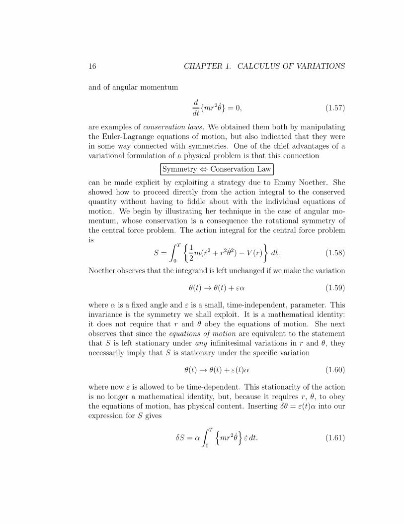
are examples of conservation laws . We obtained them both by manipulatingthe Euler-Lagrange equations of motion, but also indicated that they werein some way connected with symmetries. One of the chief advantages of avariational formulation of a physical problem is that this connection
Symmetry ⇔ Conservation Law
can be made explicit by exploiting a strategy due to Emmy Noether. Sheshowed how to proceed directly from the action integral to the conservedquantity without having to fiddle about with the individual equations ofmotion. We begin by illustrating her technique in the case of angular mo-mentum, whose conservation is a consequence the rotational symmetry ofthe central force problem. The action integral for the central force problemis
S =
∫ T
0
1
2m(r2 + r2θ2)− V (r)
dt. (1.58)
Noether observes that the integrand is left unchanged if we make the variation
θ(t)→ θ(t) + εα (1.59)
where α is a fixed angle and ε is a small, time-independent, parameter. Thisinvariance is the symmetry we shall exploit. It is a mathematical identity:it does not require that r and θ obey the equations of motion. She nextobserves that since the equations of motion are equivalent to the statementthat S is left stationary under any infinitesimal variations in r and θ, theynecessarily imply that S is stationary under the specific variation
θ(t)→ θ(t) + ε(t)α (1.60)
where now ε is allowed to be time-dependent. This stationarity of the actionis no longer a mathematical identity, but, because it requires r, θ, to obeythe equations of motion, has physical content. Inserting δθ = ε(t)α into ourexpression for S gives
δS = α
∫ T
0
mr2θ
ε dt. (1.61)

1.3. LAGRANGIAN MECHANICS 17
Note that this variation depends only on the time derivative of ε, and not εitself. This is because of the invariance of S under time-independent rota-tions. We now assume that ε(t) = 0 at t = 0 and t = T , and integrate byparts to take the time derivative off ε and put it on the rest of the integrand:
δS = −α∫
d
dt(mr2θ)
ε(t) dt. (1.62)
Since the equations of motion say that δS = 0 under all infinitesimal varia-tions, and in particular those due to any time dependent rotation ε(t)α, wededuce that the equations of motion imply that the coefficient of ε(t) mustbe zero, and so, provided r(t), θ(t), obey the equations of motion, we have
0 =d
dt(mr2θ). (1.63)
As a second illustration we derive energy (first integral) conservation forthe case that the system is invariant under time translations — meaningthat L does not depend explicitly on time. In this case the action integralis invariant under constant time shifts t → t + ε in the argument of thedynamical variable:
q(t)→ q(t + ε) ≈ q(t) + εq. (1.64)
The equations of motion tell us that that the action will be stationary underthe variation
δq(t) = ε(t)q, (1.65)
where again we now permit the parameter ε to depend on t. We insert thisvariation into
S =
∫ T
0
Ldt (1.66)
and find
δS =
∫ T
0
∂L
∂qqε+
∂L
∂q(qε+ qε)
dt. (1.67)
This expression contains undotted ε’s. Because of this the change in S is notobviously zero when ε is time independent — but the absence of any explicitt dependence in L tells us that
dL
dt=∂L
∂qq +
∂L
∂qq. (1.68)

18 CHAPTER 1. CALCULUS OF VARIATIONS
As a consequence, for time independent ε, we have
δS =
∫ T
0
εdL
dt
dt = ε[L]T0 , (1.69)
showing that the change in S comes entirely from the endpoints of the timeinterval. These fixed endpoints explicitly break time-translation invariance,but in a trivial manner. For general ε(t) we have
δS =
∫ T
0
ε(t)
dL
dt+∂L
∂qqε
dt. (1.70)
This equation is an identity. It does not rely on q obeying the equation ofmotion. After an integration by parts, taking ε(t) to be zero at t = 0, T , itis equivalent to
δS =
∫ T
0
ε(t)d
dt
L− ∂L
dt. (1.71)
Now we assume that q(t) does obey the equations of motion. The variationprinciple then says that δS = 0 for any ε(t), and we deduce that for q(t)satisfying the equations of motion we have
d
dt
L− ∂L
= 0. (1.72)
The general strategy that constitutes “Noether’s theorem” must now beobvious: we look for an invariance of the action under a symmetry trans-formation with a time-independent parameter. We then observe that if thedynamical variables obey the equations of motion, then the action principletells us that the action will remain stationary under such a variation of thedynamical variables even after the parameter is promoted to being time de-pendent. The resultant variation of S can only depend on time derivatives ofthe parameter. We integrate by parts so as to take all the time derivatives offit, and on to the rest of the integrand. Because the parameter is arbitrary,we deduce that the equations of motion tell us that that its coefficient in theintegral must be zero. This coefficient is the time derivative of something, sothis something is conserved.
1.3.3 Many degrees of freedom
The extension of the action principle to many degrees of freedom is straight-forward. As an example consider the small oscillations about equilibrium of

1.3. LAGRANGIAN MECHANICS 19
a system with N degrees of freedom. We parametrize the system in terms ofdeviations from the equilibrium position and expand out to quadratic order.We obtain a Lagrangian
L =
N∑
i,j=1
1
2Mij q
iqj − 1
2Vijq
iqj, (1.73)
where Mij and Vij are N ×N symmetric matrices encoding the inertial andpotential energy properties of the system. Now we have one equation
0 =d
dt
(∂L
∂qi
)− ∂L
∂qi=
N∑
j=1
(Mij q
j + Vijqj)
(1.74)
for each i.
1.3.4 Continuous systems
The action principle can be extended to field theories and to continuum me-chanics. Here one has a continuous infinity of dynamical degrees of freedom,either one for each point in space and time or one for each point in the mate-rial, but the extension of the variational derivative to functions of more thanone variable should possess no conceptual difficulties.
Suppose we are given an action functional S[ϕ] depending on a field ϕ(xµ)and its first derivatives
ϕµ ≡∂ϕ
∂xµ. (1.75)
Here xµ, µ = 0, 1, . . . , d, are the coordinates of d+1 dimensional space-time.It is traditional to take x0 ≡ t and the other coordinates spacelike. Supposefurther that
S[ϕ] =
∫Ldt =
∫L(xµ, ϕ, ϕµ) dd+1x, (1.76)
where L is the Lagrangian density , in terms of which
L =
∫L ddx, (1.77)
and the integral is over the space coordinates. Now
δS =
∫ δϕ(x)
∂L∂ϕ(x)
+ δ(ϕµ(x))∂L
∂ϕµ(x)
dd+1x
=
∫δϕ(x)
∂L
∂ϕ(x)− ∂
∂xµ
(∂L
∂ϕµ(x)
)dd+1x. (1.78)

20 CHAPTER 1. CALCULUS OF VARIATIONS
In going from the first line to the second, we have observed that
δ(ϕµ(x)) =∂
∂xµδϕ(x) (1.79)
and used the divergence theorem,∫
Ω
(∂Aµ
∂xµ
)dn+1x =
∫
∂Ω
AµnµdS, (1.80)
where Ω is some space-time region and ∂Ω its boundary, to integrate byparts. Here dS is the element of area on the boundary, and nµ the outwardnormal. As before, we take δϕ to vanish on the boundary, and hence thereis no boundary contribution to variation of S. The result is that
δS
δϕ(x)=
∂L∂ϕ(x)
− ∂
∂xµ
(∂L
∂ϕµ(x)
), (1.81)
and the equation of motion comes from setting this to zero. Note that a sumover the repeated coordinate index µ is implied. In practice it is easier not touse this formula. Instead, make the variation by hand—as in the followingexamples.Example: The Vibrating string . The simplest continuous dynamical systemis the transversely vibrating string. We describe the string displacement byy(x, t).
0 Ly(x,t)
Figure 1.8: Transversely vibrating string
Let us suppose that the string has fixed ends, a mass per unit lengthof ρ, and is under tension T . If we assume only small displacements fromequilibrium, the Lagrangian is
L =
∫ L
0
dx
1
2ρy2 − 1
2Ty′
2
. (1.82)

1.3. LAGRANGIAN MECHANICS 21
The dot denotes a partial derivative with respect to t, and the prime a partialderivative with respect to x. The variation of the action is
δS =
∫∫ L
0
dtdx ρy δy − Ty′δy′
=
∫∫ L
0
dtdx δy(x, t) (−ρy + Ty′′) . (1.83)
To reach the second line we have integrated by parts, and, because the endsare fixed, and therefore δy = 0 at x = 0 and L, there is no boundary term.Requiring that δS = 0 for all allowed variations δy then gives the equationof motion
ρy − Ty′′ = 0 (1.84)
This is the wave equation describing transverse waves propagating with speedc =
√T/ρ. Observe that from (1.83) we can read off the functional derivative
of S with respect to the variable y(x, t) as being
δS
δy(x, t)= −ρy(x, t) + Ty′′(x, t). (1.85)
In writing down the first integral for this continuous system, we mustreplace the sum over discrete indices by an integral:
E =∑
i
qi∂L
∂qi− L→
∫dx
y(x)
δL
δy(x)
− L. (1.86)
When computing δL/δy(x) from
L =
∫ L
0
dx
1
2ρy2 − 1
2Ty′
2
,
we must remember that it is the continuous analogue of ∂L/∂qi, and so, incontrast to what we do when computing δS/δy(x), we must treat y(x) as avariable independent of y(x). We then have
δL
δy(x)= ρy(x), (1.87)
leading to
E =
∫ L
0
dx
1
2ρy2 +
1
2Ty′
2
. (1.88)
This, as expected, is the total energy, kinetic plus potential, of the string.

22 CHAPTER 1. CALCULUS OF VARIATIONS
The energy-momentum tensor
If we consider an action of the form
S =
∫L(ϕ, ϕµ) dd+1x, (1.89)
in which L does not depend explicitly on any of the co-ordinates xµ, we mayrefine Noether’s derivation of the law of conservation total energy and obtainaccounting information about the position-dependent energy density . To dothis we make a variation of the form
ϕ(x)→ ϕ(xµ + εµ(x)) = ϕ(xµ) + εµ(x)∂µϕ+O(|ε|2), (1.90)
where ε depends on x ≡ (x0, . . . , xd). The resulting variation in S is
δS =
∫ ∂L∂ϕ
εµ∂µϕ+∂L∂ϕν
∂ν(εµ∂µϕ)
dd+1x
=
∫εµ(x)
∂
∂xν
Lδνµ −
∂L∂ϕν
∂µϕ
dd+1x. (1.91)
When ϕ satisfies the the equations of motion this δS will be zero for arbitraryεµ(x). We conclude that
∂
∂xν
Lδνµ −
∂L∂ϕν
∂µϕ
= 0. (1.92)
The (d+ 1)-by-(d+ 1) array of functions
T νµ ≡∂L∂ϕν
∂µϕ− δνµL (1.93)
is known as the canonical energy-momentum tensor because the statement
∂νTνµ = 0 (1.94)
often provides book-keeping for the flow of energy and momentum.In the case of the vibrating string, the µ = 0, 1 components of ∂νT
νµ = 0
become the two following local conservation equations:
∂
∂t
ρ
2y2 +
T
2y′2+
∂
∂x−T yy′ = 0, (1.95)

1.3. LAGRANGIAN MECHANICS 23
and∂
∂t−ρyy′+ ∂
∂x
ρ
2y2 +
T
2y′2
= 0. (1.96)
It is easy to verify that these are indeed consequences of the wave equation.They are “local” conservation laws because they are of the form
∂q
∂t+ div J = 0, (1.97)
where q is the local density, and J the flux, of the globally conserved quantityQ =
∫q ddx. In the first case, the local density q is
T 00 =
ρ
2y2 +
T
2y′2, (1.98)
which is the energy density. The energy flux is given by T 10 ≡ −T yy′, which
is the rate that a segment of string is doing work on its neighbour to the right.Integrating over x, and observing that the fixed-end boundary conditions aresuch that ∫ L
0
∂
∂x−T yy′ dx = [−T yy′]L0 = 0, (1.99)
gives usd
dt
∫ L
0
ρ
2y2 +
T
2y′2dx = 0, (1.100)
which is the global energy conservation law we obtained earlier.The physical interpretation of T 0
1 = −ρyy′, the locally conserved quan-tity appearing in (1.96) is less obvious. If this were a relativistic system,we would immediately identify
∫T 0
1 dx as the x-component of the energy-momentum 4-vector, and therefore T 0
1 as the density of x-momentum. Nowany real string will have some motion in the x direction, but the magni-tude of this motion will depend on the string’s elastic constants and otherquantities unknown to our Lagrangian. Because of this, the T 0
1 derivedfrom L cannot be the string’s x-momentum density. Instead, it is the den-sity of something called pseudo-momentum. The distinction between trueand pseudo-momentum is best appreaciated by considering the correspond-ing Noether symmetry. The symmetry associated with Newtonian momen-tum is the invariance of the action integral under an x translation of theentire apparatus: the string, and any wave on it. The symmetry associ-ated with pseudo-momentum is the invariance of the action under a shift

24 CHAPTER 1. CALCULUS OF VARIATIONS
y(x) → y(x − a) of the location of the wave on the string — the string it-self not being translated. Newtonian momentum is conserved if the ambientspace is translationally invariant. Pseudo-momentum is conserved only if thestring is translationally invariant — i.e. if ρ and T are position independent.A failure to realize that the presence of a medium (here the string) requires usto distinguish between these two symmetries is the origin of much confusioninvolving “wave momentum.”
Maxwell’s equations
Michael Faraday and and James Clerk Maxwell’s description of electromag-netism in terms of dynamical vector fields gave us the first modern fieldtheory. D’Alembert and Maupertuis would have been delighted to discoverthat the famous equations of Maxwell’s A Treatise on Electricity and Mag-netism (1873) follow from an action principle. There is a slight complicationstemming from gauge invariance but, as long as we are not interested in ex-hibiting the covariance of Maxwell under Lorentz transformations, we cansweep this under the rug by working in the axial gauge, where the scalarelectric potential does not appear.
We will start from Maxwell’s equations
divB = 0,
curlE = −∂B∂t,
curlH = J+∂D
∂t,
divD = ρ, (1.101)
and show that they can be obtained from an action principle. For conveniencewe shall use natural units in which µ0 = ε0 = 1, and so c = 1 and D ≡ Eand B ≡ H.
The first equation divB = 0 contains no time derivatives. It is a con-straint which we satisfy by introducing a vector potentialA such thatB =curlA.If we set
E = −∂A∂t
, (1.102)
then this automatically implies Faraday’s law of induction
curlE = −∂B∂t. (1.103)

1.3. LAGRANGIAN MECHANICS 25
We now guess that the Lagrangian is
L =
∫d3x
[1
2
E2 −B2
+ J ·A
]. (1.104)
The motivation is that L looks very like T − V if we regard 12E2 ≡ 1
2A2 as
being the kinetic energy and 12B2 = 1
2(curlA)2 as being the potential energy.
The term in J represents the interaction of the fields with an external currentsource. In the axial gauge the electric charge density ρ does not appear inthe Lagrangian. The corresponding action is therefore
S =
∫Ldt =
∫∫d3x
[1
2A2 − 1
2(curlA)2 + J ·A
]dt. (1.105)
Now vary A to A+ δA, whence
δS =
∫∫d3x
[−A · δA− (curlA) · (curl δA) + J · δA
]dt. (1.106)
Here, we have already removed the time derivative from δA by integratingby parts in the time direction. Now we do the integration by parts in thespace directions by using the identity
div (δA× (curlA)) = (curlA) · (curl δA)− δA · (curl (curlA)) (1.107)
and taking δA to vanish at spatial infinity, so the surface term, which wouldcome from the integral of the total divergence, is zero. We end up with
δS =
∫∫d3x
δA ·
[−A− curl (curlA) + J
]dt. (1.108)
Demanding that the variation of S be zero thus requires
∂2A
∂t2= −curl (curlA) + J, (1.109)
or, in terms of the physical fields,
curlB = J+∂E
∂t. (1.110)
This is Ampere’s law, as modified by Maxwell so as to include the displace-ment current.

26 CHAPTER 1. CALCULUS OF VARIATIONS
How do we deal with the last Maxwell equation, Gauss’ law, which assertsthat divE = ρ? If ρ were equal to zero, this equation would hold if divA = 0,i.e. if A were solenoidal. In this case we might be tempted to impose theconstraint divA = 0 on the vector potential, but doing so would undo allour good work, as we have been assuming that we can vary A freely.
We notice, however, that the three Maxwell equations we already possesstell us that
∂
∂t(divE− ρ) = div (curlB)−
(div J+
∂ρ
∂t
). (1.111)
Now div (curlB) = 0, so the left-hand side is zero provided charge is con-served, i.e. provided
ρ+ div J = 0. (1.112)
We assume that this is so. Thus, if Gauss’ law holds initially, it holds eter-nally. We arrange for it to hold at t = 0 by imposing initial conditions onA. We first choose A|t=0 by requiring it to satisfy
B|t=0 = curl (A|t=0) . (1.113)
The solution is not unique, because may we add any ∇φ to A|t=0, but thisdoes not affect the physical E and B fields. The initial “velocities” A|t=0
are then fixed uniquely by A|t=0 = −E|t=0, where the initial E satisfiesGauss’ law. The subsequent evolution of A is then uniquely determined byintegrating the second-order equation (1.109).
The first integral for Maxwell is
E =3∑
i=1
∫d3x
Ai
δL
δAi
− L
=
∫d3x
[1
2
E2 +B2
− J ·A
]. (1.114)
This will be conserved if J is time independent. If J = 0, it is the total fieldenergy.
Suppose J is neither zero nor time independent. Then, looking back atthe derivation of the time-independence of the first integral, we see that if Ldoes depend on time, we instead have
dE
dt= −∂L
∂t. (1.115)

1.3. LAGRANGIAN MECHANICS 27
In the present case we have
−∂L∂t
= −∫
J ·A d3x, (1.116)
so that
−∫
J ·A d3x =dE
dt=
d
dt(Field Energy)−
∫ J · A+ J ·A
d3x. (1.117)
Thus, cancelling the duplicated term and using E = −A, we find
d
dt(Field Energy) = −
∫J · E d3x. (1.118)
Now∫J · (−E) d3x is the rate at which the power source driving the current
is doing work against the field. The result is therefore physically sensible.
Continuum mechanics
Because the mechanics of discrete objects can be derived from an actionprinciple, it seems obvious that so must the mechanics of continua. This iscertainly true if we use the Lagrangian description where we follow the his-tory of each particle composing the continuous material as it moves throughspace. In fluid mechanics it is more natural to describe the motion by usingthe Eulerian description in which we focus on what is going on at a partic-ular point in space by introducing a velocity field v(r, t). Eulerian actionprinciples can still be found, but they seem to be logically distinct from theLagrangian mechanics action principle, and mostly were not discovered untilthe 20th century.
We begin by showing that Euler’s equation for the irrotational motionof an inviscid compressible fluid can be obtained by applying the actionprinciple to a functional
S[φ, ρ] =
∫dt d3x
ρ∂φ
∂t+
1
2ρ(∇φ)2 + u(ρ)
, (1.119)
where ρ is the mass density and the flow velocity is determined from thevelocity potential φ by v = ∇φ. The function u(ρ) is the internal energydensity.

28 CHAPTER 1. CALCULUS OF VARIATIONS
Varying S[φ, ρ] with respect to ρ is straightforward, and gives a timedependent generalization of (Daniel) Bernoulli’s equation
∂φ
∂t+
1
2v2 + h(ρ) = 0. (1.120)
Here h(ρ) ≡ du/dρ, is the specific enthalpy.1 Varying with respect to φrequires an integration by parts, based on
div (ρ δφ∇φ) = ρ(∇δφ) · (∇φ) + δφ div (ρ∇φ), (1.121)
and gives the equation of mass conservation
∂ρ
∂t+ div (ρv) = 0. (1.122)
Taking the gradient of Bernoulli’s equation, and using the fact that for po-tential flow the vorticity ω ≡ curlv is zero and so ∂ivj = ∂jvi, we find that
∂v
∂t+ (v · ∇)v = −∇h. (1.123)
We now introduce the pressure P , which is related to h by
h(P ) =
∫ P
0
dP
ρ(P ). (1.124)
We see that ρ∇h = ∇P , and so obtain Euler’s equation
ρ
(∂v
∂t+ (v · ∇)v
)= −∇P. (1.125)
For future reference, we observe that combining the mass-conservation equa-tion
∂tρ+ ∂j ρvj = 0 (1.126)
with Euler’s equationρ(∂tvi + vj∂jvi) = −∂iP (1.127)
1The enthalpy H = U + PV per unit mass. In general u and h will be functions ofboth the density and the specific entropy. By taking u to depend only on ρ we are tacitlyassuming that specific entropy is constant. This makes the resultant flow barotropic,meaning that the pressure is a function of the density only.

1.4. VARIABLE END POINTS 29
yields
∂t ρvi+ ∂j ρvivj + δijP = 0, (1.128)
which expresses the local conservation of momentum. The quantity
Πij = ρvivj + δijP (1.129)
is the momentum-flux tensor , and is the j-th component of the flux of thei-th component pi = ρvi of momentum density.
The relations h = du/dρ and ρ = dP/dh show that P and u are relatedby a Legendre transformation: P = ρh− u(ρ). From this, and the Bernoulliequation, we see that the integrand in the action (1.119) is equal to minusthe pressure:
−P = ρ∂φ
∂t+
1
2ρ(∇φ)2 + u(ρ). (1.130)
This Eulerian formulation cannot be a “follow the particle” action prin-ciple in a clever disguise. The mass conservation law is only a consequenceof the equation of motion, and is not built in from the beginning as a con-straint. Our variations in φ are therefore conjuring up new matter ratherthan merely moving it around.
1.4 Variable End Points
We now relax our previous assumption that all boundary or surface termsarising from integrations by parts may be ignored. We will find that variationprinciples can be very useful for working out what boundary conditions weshould impose on our differential equations.
Consider the problem of building a railway across a parallel sided isthmus.

30 CHAPTER 1. CALCULUS OF VARIATIONS
)y(x1
y(x2)
x
y
Figure 1.9: Railway across isthmus.
Suppose that the cost of construction is proportional to the length of thetrack, but the cost of sea transport being negligeable, we may locate theterminal seaports wherever we like. We therefore wish to minimize the length
L[y] =
∫ x2
x1
√1 + (y′)2dx, (1.131)
by allowing both the path y(x) and the endpoints y(x1) and y(x2) to vary.Then
L[y + δy]− L[y] =
∫ x2
x1
(δy′)y′√
1 + (y′)2dx
=
∫ x2
x1
d
dx
(δy
y′√1 + (y′)2
)− δy d
dx
(y′√
1 + (y′)2
)dx
= δy(x2)y′(x2)√1 + (y′)2
− δy(x1)y′(x1)√1 + (y′)2
−∫ x2
x1
δyd
dx
(y′√
1 + (y′)2
)dx. (1.132)
We have stationarity when bothi) the coefficient of δy(x) in the integral,
− d
dx
(y′√
1 + (y′)2
), (1.133)
is zero. This requires that y′ =const., i.e. the track should be straight.

1.4. VARIABLE END POINTS 31
ii) The coefficients of δy(x1) and δy(x2) vanish. For this we need
0 =y′(x1)√1 + (y′)2
=y′(x2)√1 + (y′)2
. (1.134)
This in turn requires that y′(x1) = y′(x2) = 0.The integrated-out bits have determined the boundary conditions that are tobe imposed on the solution of the differential equation. In the present casethey require us to build perpendicular to the coastline, and so we go straightacross the isthmus. When boundary conditions are obtained from endpointvariations in this way, they are called natural boundary conditions .Example: Sliding String . A massive string of linear density ρ is stretchedbetween two smooth posts separated by distance 2L. The string is undertension T , and is free to slide up and down the posts. We consider only asmall deviations of the string from the horizontal.
x
y
+L−L
Figure 1.10: Sliding string.
As we saw earlier, the Lagrangian for a stretched string is
L =
∫ L
−L
1
2ρy2 − 1
2T (y′)2
dx. (1.135)
Now, Lagrange’s principle says that the equation of motion is found by re-quiring the action
S =
∫ tf
ti
Ldt (1.136)
to be stationary under variations of y(x, t) that vanish at the initial and finaltimes, ti and tf . It does not demand that δy vanish at ends of the string,x = ±L. So, when we make the variation, we must not assume this. Taking

32 CHAPTER 1. CALCULUS OF VARIATIONS
care not to discard the results of the integration by parts in the x direction,we find
δS =
∫ tf
ti
∫ L
−Lδy(x, t) −ρy + Ty′′ dxdt−
∫ tf
ti
δy(L, t)Ty′(L) dt
+
∫ tf
ti
δy(−L, t)Ty′(−L) dt. (1.137)
The equation of motion, which arises from the variation within the interval,is therefore the wave equation
ρy − Ty′′ = 0. (1.138)
The boundary conditions, which come from the variations at the endpoints,are
y′(L, t) = y′(−L, t) = 0, (1.139)
at all times t. These are the physically correct boundary conditions, becauseany up-or-down component of the tension would provide a finite force on aninfinitesimal mass. The string must therefore be horizontal at its endpoints.
Example: Bead and String . Suppose now that a bead of mass M is free toslide up and down the y axis,
x
y
y(0)
0 L
Figure 1.11: A bead connected to a string.
and is is attached to the x = 0 end of our string. The Lagrangian for thestring-bead contraption is
L =1
2M [y(0)]2 +
∫ L
0
1
2ρy2 − 1
2Ty′2
dx. (1.140)
1.4. VARIABLE END POINTS 33
Here, as before, ρ is the mass per unit length of the string and T is its tension.The end of the string at x = L is fixed. By varying the action S =
∫Ldt,
and taking care not to throw away the boundary part at x = 0 we find that
δS =
∫ tf
ti
[Ty′ −My]x=0 δy(0, t) dt+
∫ tf
ti
∫ L
0
Ty′′ − ρy δy(x, t) dxdt.(1.141)
The Euler-Lagrange equations are therefore
ρy(x)− Ty′′(x) = 0, 0 < x < L,
My(0)− Ty′(0) = 0, y(L) = 0. (1.142)
The boundary condition at x = 0 is the equation of motion for the bead. Itis clearly correct, because Ty′(0) is the vertical component of the force thatthe string tension exerts on the bead.
These examples led to boundary conditions that we could easily havefigured out for ourselves without the variational principle. The next exam-ple shows that a variational formulation can be exploited to obtain a set ofboundary conditions that might be difficult to write down by purely “physi-cal” reasoning.
y
x
0
0P
h(x,t)
ρ
g
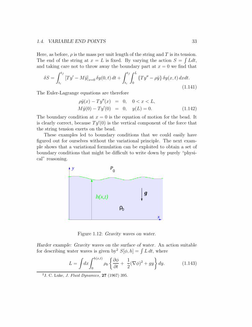
Figure 1.12: Gravity waves on water.
Harder example: Gravity waves on the surface of water. An action suitablefor describing water waves is given by2 S[φ, h] =
∫Ldt, where
L =
∫dx
∫ h(x,t)
0
ρ0
∂φ
∂t+
1
2(∇φ)2 + gy
dy. (1.143)
2J. C. Luke, J. Fluid Dynamics, 27 (1967) 395.

34 CHAPTER 1. CALCULUS OF VARIATIONS
Here φ is the velocity potential and ρ0 is the density of the water. The densitywill not be varied because the water is being treated as incompressible. Asbefore, the flow velocity is given by v = ∇φ. By varying φ(x, y, t) and thedepth h(x, t), and taking care not to throw away any integrated-out parts ofthe variation at the physical boundaries, we obtain:
∇2φ = 0, within the fluid.∂φ
∂t+
1
2(∇φ)2 + gy = 0, on the free surface.
∂φ
∂y= 0, on y = 0.
∂h
∂t− ∂φ
∂y+∂h
∂x
∂φ
∂x= 0, on the free surface. (1.144)
The first equation comes from varying φ within the fluid, and it simplyconfirms that the flow is incompressible, i.e. obeys div v = 0. The secondcomes from varying h, and is the Bernoulli equation stating that we haveP = P0 (atmospheric pressure) everywhere on the free surface. The third,from the variation of φ at y = 0, states that no fluid escapes through thelower boundary.
Obtaining and interpreting the last equation, involving ∂h/∂t, is some-what trickier. It comes from the variation of φ on the upper boundary. Thevariation of S due to δφ is
δS =
∫ρ0
∂
∂tδφ+
∂
∂x
(δφ∂φ
∂x
)+
∂
∂y
(δφ∂φ
∂y
)− δφ∇2φ
dtdxdy.
(1.145)The first three terms in the integrand constitute the three-dimensional di-vergence div (δφΦ), where, listing components in the order t, x, y,
Φ =
[1,∂φ
∂x,∂φ
∂y
]. (1.146)
The integrated-out part on the upper surface is therefore∫(Φ · n)δφ d|S|.
Here, the outward normal is
n =
(1 +
(∂h
∂t
)2
+
(∂h
∂x
)2)−1/2 [
−∂h∂t,−∂h
∂x, 1
], (1.147)

1.4. VARIABLE END POINTS 35
and the element of area
d|S| =(1 +
(∂h
∂t
)2
+
(∂h
∂x
)2)1/2
dtdx. (1.148)
The boundary variation is thus
δS|y=h = −∫
∂h
∂t− ∂φ
∂y+∂h
∂x
∂φ
∂x
δφ(x, h(x, t), t
)dxdt. (1.149)
Requiring this variation to be zero for arbitrary δφ(x, h(x, t), t
)leads to
∂h
∂t− ∂φ
∂y+∂h
∂x
∂φ
∂x= 0. (1.150)
This last boundary condition expresses the geometrical constraint that thesurface moves with the fluid it bounds, or, in other words, that a fluid particleinitially on the surface stays on the surface. To see that this is so, definef(x, y, t) = h(x, t) − y. The free surface is then determined by f(x, y, t) =0. Because the surface particles are carried with the flow, the convectivederivative of f ,
df
dt≡ ∂f
∂t+ (v · ∇)f, (1.151)
must vanish on the free surface. Using v = ∇φ and the definition of f , thisreduces to
∂h
∂t+∂φ
∂x
∂h
∂x− ∂φ
∂y= 0, (1.152)
which is indeed the last boundary condition.

36 CHAPTER 1. CALCULUS OF VARIATIONS
1.5 Lagrange Multipliers
y
x
Figure 1.13: Road on hill.
Figure 1.13 shows the contour map of a hill of height h = f(x, y). Thehill traversed by a road whose points satisfy the equation g(x, y) = 0. Ourchallenge is to use the data f(x, y) and g(x, y) to find the highest point onthe road.
When r changes by dr = (dx, dy), the height f changes by
df = ∇f · dr, (1.153)
where ∇f = (∂xf, ∂yf). The highest point, being a stationary point, willhave df = 0 for all displacements dr that stay on the road — that is forall dr such that dg = 0. Thus ∇f · dr must be zero for those dr such that0 = ∇g · dr. In other words, at the highest point ∇f will be orthogonal toall vectors that are orthogonal to ∇g. This is possible only if the vectors ∇fand ∇g are parallel, and so ∇f = λ∇g for some λ.
To find the stationary point, therefore, we solve the equations
∇f − λ∇g = 0,
g(x, y) = 0, (1.154)
simultaneously.Example: Let f = x2 + y2 and g = x + y − 1. Then ∇f = 2(x, y) and∇g = (1, 1). So
2(x, y)− λ(1, 1) = 0, ⇒ (x, y) =λ
2(1, 1)

1.5. LAGRANGE MULTIPLIERS 37
x+ y = 1, ⇒ λ = 1, =⇒ (x, y) = (1
2,1
2).
When there are n constraints, g1 = g2 = · · · = gn = 0, we want ∇f to liein
(< ∇gi >⊥)⊥ =< ∇gi >, (1.155)
where < ei > denotes the space spanned by the vectors ei and < ei >⊥ is
the its orthogonal complement. Thus ∇f lies in the space spanned by thevectors ∇gi, so there must exist n numbers λi such that
∇f =n∑
i=1
λi∇gi. (1.156)
The numbers λi are called Lagrange multipliers . We can therefore regard ourproblem as one of finding the stationary points of an auxilliary function
F = f −∑
i
λigi, (1.157)
with the n undetermined multipliers λi, i = 1, . . . , n, subsequently being fixedby imposing the n requirements that gi = 0, i = 1, . . . , n.Example: Find the stationary points of
F (x) =1
2x ·Ax =
1
2xiAijxj (1.158)
on the surface x · x = 1. Here Aij is a symmetric matrix.Solution: We look for stationary points of
G(x) = F (x)− 1
2λ|x|2. (1.159)
The derivatives we need are
∂F
∂xk=
1
2δkiAijxj +
1
2xiAijδjk
= Akjxj , (1.160)
and∂
∂xk
(λ
2xjxj
)= λxk. (1.161)
38 CHAPTER 1. CALCULUS OF VARIATIONS
Thus, the stationary points must satisfy
Akjxj = λxk,
xixi = 1, (1.162)
and so are the normalized eigenvectors of the matrix A. The Lagrangemultiplier at each stationary point is the corresponding eigenvalue.Example: Statistical Mechanics. Let Γ denote the classical phase space ofa mechanical system of n particles governed by Hamiltonian H(p, q). LetdΓ be the Liouville measure d3np d3nq. In statistical mechanics we workwith a probability density ρ(p, q) such that ρ(p, q)dΓ is the probability ofthe system being in a state in the small region dΓ. The entropy associatedwith the probability distribution is the functional
S[ρ] = −∫
Γ
ρ ln ρ dΓ. (1.163)
We wish to find the ρ(p, q) that maximizes the entropy for a given energy
〈E〉 =∫
Γ
ρH dΓ. (1.164)
We cannot vary ρ freely as we should preserve both the energy and thenormalization condition ∫
Γ
ρ dΓ = 1 (1.165)
that is required of any probability distribution. We therefore introduce twoLagrange multipliers, 1 + α and β, to enforce the normalization and energyconditions, and look for stationary points of
F [ρ] =
∫
Γ
−ρ ln ρ+ (α + 1)ρ− βρH dΓ. (1.166)
Now we can vary ρ freely, and hence find that
δF =
∫
Γ
− ln ρ+ α− βH δρ dΓ. (1.167)
Requiring this to be zero gives us
ρ(p, q) = eα−βH(p,q), (1.168)

1.5. LAGRANGE MULTIPLIERS 39
where α, β are determined by imposing the normalization and energy con-straints. This probability density is known as the canonical distribution, andthe parameter β is the inverse temperature β = 1/T .Example: The Catenary. At last we have the tools to solve the problem ofthe hanging chain of fixed length. We wish to minimize the potential energy
E[y] =
∫ L
−Ly√1 + (y′)2dx, (1.169)
subject to the constraint
l[y] =
∫ L
−L
√1 + (y′)2dx = const., (1.170)
where the constant is the length of the chain. We introduce a Lagrangemultiplier λ and find the stationary points of
F [y] =
∫ L
−L(y − λ)
√1 + (y′)2dx, (1.171)
so, following our earlier methods, we find
y = λ+ κ cosh(x+ a)
κ. (1.172)
We choose κ, λ, a to fix the two endpoints (two conditions) and the length(one condition).Example: Sturm-Liouville Problem. We wish to find the stationary pointsof the quadratic functional
J [y] =
∫ x2
x1
1
2
p(x)(y′)2 + q(x)y2
dx, (1.173)
subject to the boundary conditions y(x) = 0 at the endpoints x1, x2 and thenormalization
K[y] =
∫ x2
x1
y2 dx = 1. (1.174)
Taking the variation of J − (λ/2)K, we find
δJ =
∫ x2
x1
−(py′)′ + qy − λy δy dx. (1.175)

40 CHAPTER 1. CALCULUS OF VARIATIONS
Stationarity therefore requires
−(py′)′ + qy = λy, y(x1) = y(x2) = 0. (1.176)
This is the Sturm-Liouville eigenvalue problem. It is an infinite dimensionalanalogue of the F (x) = 1
2x ·Ax problem.
Example: Irrotational Flow Again. Consider the action functional
S[v, φ, ρ] =
∫ 1
2ρv2 − u(ρ) + φ
(∂ρ
∂t+ div ρv
)dtd3x (1.177)
This is similar to our previous action for the irrotational barotropic flow of aninviscid fluid, but here v is an independent variable and we have introducedinfinitely many Lagrange multipliers φ(x, t), one for each point of space-time,so as to enforce the equation of mass conservation ρ+div ρv = 0 everywhere,and at all times. Equating δS/δv to zero gives v = ∇φ, and so these Lagrangemultipliers become the velocity potential as a consequence of the equationsof motion. The Bernoulli and Euler equations now follow almost as before.Because the equation v = ∇φ does not involve time derivatives, this isone of the cases where it is legitimate to substitute a consequence of theaction principle back into the action. If we do this, we recover our previousformulation.
1.6 Maximum or Minimum?
We have provided many examples of stationary points in function space. Wehave said almost nothing about whether these stationary points are maximaor minima. There is a reason for this: investigating the character of thestationary point requires the computation of the second functional derivative.
δ2J
δy(x1)δy(x2)
and the use of the functional version of Taylor’s theorem to expand aboutthe stationary point y(x):
J [y + εη] = J [y] + ε
∫η(x)
δJ
δy(x)
∣∣∣∣y
dx
+ε2
2
∫η(x1)η(x2)
δ2J
δy(x1)δy(x2)
∣∣∣∣y
dx1dx2 + · · · .
(1.178)
1.6. MAXIMUM OR MINIMUM? 41
Since y(x) is a stationary point, the term with δJ/δy(x)|y vanishes. Whethery(x) is a maximum, a minimum, or a saddle therefore depends on the numberof positive and negative eigenvalues of δ2J/δ(y(x1))δ(y(x2)), a matrix witha continuous infinity of rows and columns—these being labeled by x1 andx2 repectively. It is not easy to diagonalize a continuously infinite matrix!Consider, for example, the functional
J [y] =
∫ b
a
1
2
p(x)(y′)2 + q(x)y2
dx, (1.179)
with y(a) = y(b) = 0. Here, as we already know,
δJ
δy(x)= Ly ≡ − d
dx
(p(x)
d
dxy(x)
)+ q(x)y(x), (1.180)
and, except in special cases, this will be zero only if y(x) ≡ 0. We mightreasonably expect the second derivative to be
δ
δy(Ly)
?= L, (1.181)
where L is the Sturm-Liouville differential operator
L = − d
dx
(p(x)
d
dx
)+ q(x). (1.182)
How can a differential operator be a matrix like δ2J/δ(y(x1))δ(y(x2))?We can formally compute the second derivative by exploiting the Dirac
delta “function” δ(x) which has the property that
y(x2) =
∫δ(x2 − x1)y(x1) dx1. (1.183)
Thus
δy(x2) =
∫δ(x2 − x1)δy(x1) dx1, (1.184)
from which we read off that
δy(x2)
δy(x1)= δ(x2 − x1). (1.185)

42 CHAPTER 1. CALCULUS OF VARIATIONS
Using (1.185), we find that
δ
δy(x1)
(δJ
δy(x2)
)= − d
dx2
(p(x2)
d
dx2δ(x2 − x1)
)+q(x2)δ(x2−x1). (1.186)
How are we to make sense of this expression? We begin in the next chapterwhere we explain what it means to differentiate δ(x), and show that (1.186)does indeed correspond to the differential operator L. In subsequent chap-ters we explore the manner in which differential operators and matrices arerelated. We will learn that just as some matrices can be diagonalized so cansome differential operators, and that the class of diagonalizable operatorsincludes (1.182).
If all the eigenvalues of L are positive, our stationary point was a min-imum. For each negative eigenvalue, there is direction in function space inwhich J [y] decreases as we move away from the stationary point.
1.7 Further Exercises and Problems
Here is a collection of problems relating to the calculus of variations. Somedate back to the 16th century, others are quite recent in origin.
Exercise 1.1: A smooth path in the x-y plane is given by r(t) = (x(t), y(t))with r(0) = a, and r(1) = b. The length of the path from a to b is therefore.
S[r] =
∫ 1
0
√x2 + y2 dt,
where x ≡ dx/dt, y ≡ dy/dt. Write down the Euler-Lagrange conditions forS[r] to be stationary under small variations of the path that keep the endpointsfixed, and hence show that the shortest path between two points is a straightline.
Exercise 1.2: Fermat’s principle. A medium is characterised optically byits refractive index n, such that the speed of light in the medium is c/n.According to Fermat (1657), the path taken by a ray of light between anytwo points makes stationary the travel time between those points. Assumethat the ray propagates in the x, y plane in a layered medium with refractiveindex n(x). Use Fermat’s principle to establish Snell’s law in its general formn(x) sinψ = constant by finding the equation giving the stationary paths y(x)for
F1[y] =
∫n(x)
√1 + y′2dx.

1.7. FURTHER EXERCISES AND PROBLEMS 43
(Here the prime denotes differentiation with respect to x.) Repeat this exercisefor the case that n depends only on y and find a similar equation for thestationary paths of
F2[y] =
∫n(y)
√1 + y′2dx.
By using suitable definitions of the angle of incidence ψ in each case, showthat the two formulations of the problem give physically equivalent answers.In the second formulation you will find it easiest to use the first integral ofEuler’s equation.
Problem 1.3: Hyperbolic Geometry. This problem introduces a version of thePoincare model for the non-Euclidean geometry of Lobachevski.
a) Show that the stationary paths for the functional
F3[y] =
∫1
y
√1 + y′2dx,
with y(x) restricted to lying in the upper half plane are semi-circles ofarbitrary radius and with centres on the x axis. These paths are thegeodesics, or minimum length paths, in a space with Riemann metric
ds2 =1
y2(dx2 + dy2), y > 0.
b) Show that if we call these geodesics “lines”, then one and only one linecan be drawn though two given points.
c) Two lines are said to be parallel if, and only if, they meet at “infinity”,i.e. on the x axis. (Verify that the x axis is indeed infinitely far from anypoint with y > 0.) Show that given a line q and a point A not lying onthat line, that there are two lines passing through A that are parallel toq, and that between these two lines lies a pencil of lines passing throughA that never meet q.
Problem 1.4: Elastic Rods. The elastic energy per unit length of a bent steelrod is given by 1
2Y I/R2. Here R is the radius of curvature due to the bending,
Y is the Young’s modulus of the steel and I =∫∫y2dxdy is the moment
of inertia of the rod’s cross section about an axis through its centroid andperpendicular to the plane in which the rod is bent. If the rod is only slightlybent into the yz plane and lies close to the z axis, show that this elastic energycan be approximated as
U [y] =
∫ L
0
1
2Y I(y′′)2dz,

44 CHAPTER 1. CALCULUS OF VARIATIONS
where the prime denotes differentiation with respect to z and L is the lengthof the rod. We will use this approximate energy functional to discuss twopractical problems.
L
Mg
Mg
a) b)
Figure 1.14: A rod used as: a) a column, b) a cantilever.
a) Euler’s problem: the buckling of a slender column. The rod is used asa column which supports a compressive load Mg directed along the zaxis (which is vertical). Show that when the rod buckles slighly (i.e.deforms with both ends remaining on the z axis) the total energy, in-cluding the gravitational potential energy of the loading mass M , can beapproximated by
U [y] =
∫ L
0
Y I
2
(y′′)2 − Mg
2
(y′)2dz.
By considering small deformations of the form
y(z) =
∞∑
n=1
an sinnπz
L
show that the column is unstable to buckling and collapse if Mg ≥π2Y I/L2.
b) Leonardo da Vinci’s problem: the light cantilever. Here we take the zaxis as horizontal and the y axis as being vertical. The rod is used asa beam or cantilever and is fixed into a wall so that y(0) = 0 = y′(0).A weight Mg is hung from the end z = L and the beam sags in the −ydirection. We wish to find y(z) for 0 < z < L. We will ignore the weightof the beam itself.• Write down the complete expression for the energy, including the
gravitational potential energy of the weight.

1.7. FURTHER EXERCISES AND PROBLEMS 45
• Find the differential equation and boundary conditions at z = 0, Lthat arise from minimizing the total energy. In doing this take carenot to throw away any term arising from the integration by parts.You may find the following identity to be of use:
d
dz(f ′g′′ − fg′′′) = f ′′g′′ − fg′′′′.
• Solve the equation. You should find that the displacement of theend of the beam is y(L) = −1
3MgL3/Y I.
Exercise 1.5: Suppose that an elastic body Ω of density ρ is slightly deformedso that the point that was at cartesian co-ordinate xi is moved to xi + ηi(x).We define the resulting strain tensor eij by
eij =1
2
(∂ηj∂xi
+∂ηi∂xj
).
It is automatically symmetric in its indices. The Lagrangian for small-amplitudeelastic motion of the body is
L[η] =
∫
Ω
1
2ρη2i −
1
2eijcijklekl
d3x.
Here, cijkl is the tensor of elastic constants, which has the symmetries
cijkl = cklij = cjikl = cijlk.
By varying the ηi, show that the equation of motion for the body is
ρ∂2ηi∂t2− ∂
∂xjσji = 0,
where
σij = cijklekl
is the stress tensor . Show that variations of ηi on the boundary ∂Ω give asboundary conditions
σijnj = 0,
where ni are the components of the outward normal on ∂Ω.

46 CHAPTER 1. CALCULUS OF VARIATIONS
ψ
ψ
s
aπ4
Figure 1.15: Weighted line.
Problem 1.6:The catenary revisited. We can describe a catenary curve inparametric form as x(s), y(s), where s is the arc-length. The potential en-
ergy is then simply∫ L0 ρgy(s)ds where ρ is the mass per unit length of the
hanging chain. The x, y are not independent functions of s, however, becausex2 + y2 = 1 at every point on the curve. Here a dot denotes a derivative withrespect to s.
a) Introduce infinitely many Lagrange multipliers λ(s) to enforce the x2 + y2
constraint, one for each point s on the curve. From the resulting func-tional derive two coupled equations describing the catenary, one for x(s)and one for y(s). By thinking about the forces acting on a small sectionof the cable, and perhaps by introducing the angle ψ where x = cosψ andy = sinψ, so that s and ψ are intrinsic coordinates for the curve, inter-pret these equations and show that λ(s) is proportional to the position-dependent tension T (s) in the chain.
b) You are provided with a light-weight line of length πa/2 and some leadshot of total mass M . By using equations from the previous part (suit-ably modified to take into account the position dependent ρ(s)) or oth-erwise, determine how the lead should be distributed along the line if theloaded line is to hang in an arc of a circle of radius a (see figure 1.15)when its ends are attached to two points at the same height.
Problem 1.7: Another model for Lobachevski geometry (see exercise 1.3)is the Poincare disc. This space consists of the interior of the unit discD2 = (x, y) ∈ R2 : x2 + y2 ≤ 1 equipped with Riemann metric
ds2 =dx2 + dy2
(1− x2 − y2)2 .

1.7. FURTHER EXERCISES AND PROBLEMS 47
The geodesic paths are found by minimizing the arc-length functional
s[r] ≡∫ds =
∫ 1
1− x2 − y2√x2 + y2
dt,
where r(t) = (x(t), y(t)) and a dot indicates a derivative with respect to theparameter t.
y
xO
D2
P
R
Q X
r
Figure 1.16: The Poincare disc of exercise 1.7. The radius OP of the Poincaredisc is unity, while the radius of the geodesic arc PQR is PX = QX = RX =R. The distance between the centres of the disc and arc is OX = x0. Yourtask in part c) is to show that ∠OPX = ∠ORX = 90.
a) Either by manipulating the two Euler-Lagrange equations that give theconditions for s[r] to be stationary under variations in r(t), or, more effi-ciently, by observing that s[r] is invariant under the infinitesimal rotation
δx = εy
δy = −εx
and applying Noether’s theorem, show that the parameterised geodesicsobey
d
dt
(1
1− x2 − y2xy − yx√x2 + y2
)= 0.
b) Given a point (a, b) within D2, and a direction through it, show thatthe equation you derived in part a) determines a unique geodesic curve

48 CHAPTER 1. CALCULUS OF VARIATIONS
passing through (a, b) in the given direction, but does not determine theparametrization of the curve.
c) Show that there exists a solution to the equation in part a) in the form
x(t) = R cos t+ x0
y(t) = R sin t.
Find a relation between x0 and R, and from it deduce that the geodesicsare circular arcs that cut the bounding unit circle (which plays the roleof the line at infinity in the Lobachevski plane) at right angles.
Exercise 1.8: The Lagrangian for a particle of charge q is
L[x, x] =1
2mx2 − qφ(x) + qx ·A(x).
Show that Lagrange’s equation leads to
mx = q(E+ x×B),
where
E = −∇φ− ∂A
∂t, B = curlA.
Exercise 1.9: Consider the action functional
S[ω,p, r] =
∫ (1
2I1ω
21 +
1
2I2ω
22 +
1
2I3ω
23 + p · (r+ ω × r)
dt,
where r and p are time-dependent three-vectors, as is ω = (ω1, ω2, ω3), Applythe action principle to obtain the equations of motion for r,p,ω and showthat they lead to Euler’s equations
I1ω1 − (I2 − I3)ω2ω3 = 0,
I2ω2 − (I3 − I1)ω3ω1 = 0,
I3ω3 − (I1 − I2)ω1ω2 = 0.
governing the angular velocity of a freely-rotating rigid body.
Problem 1.10: Piano String. A elastic piano string can vibrate both trans-versely and longitudinally, and the two vibrations influence one another. ALagrangian that takes into account the lowest-order effect of stretching on thelocal string tension, and can therefore model this coupled motion, is
L[ξ, η] =
∫dx
1
2ρ0
[(∂ξ
∂t
)2
+
(∂η
∂t
)2]− λ
2
[τ0λ
+∂ξ
∂x+
1
2
(∂η
∂x
)2]2 .

1.7. FURTHER EXERCISES AND PROBLEMS 49
η
ξ
x
y
Figure 1.17: Vibrating piano string.
Here ξ(x, t) is the longitudinal displacement and η(x, t) the transverse dis-placement of the string. Thus, the point that in the undisturbed string hadco-ordinates [x, 0] is moved to the point with co-ordinates [x+ ξ(x, t), η(x, t)].The parameter τ0 represents the tension in the undisturbed string, λ is theproduct of Young’s modulus and the cross-sectional area of the string, and ρ0is the mass per unit length.
a) Use the action principle to derive the two coupled equations of motion,
one involving∂2ξ
∂t2and one involving
∂2η
∂t2.
b) Show that when we linearize these two equations of motion, the longi-tudinal and transverse motions decouple. Find expressions for the lon-gitudinal (cL) and transverse (cT ) wave velocities in terms of τ0, ρ0 andλ.
c) Assume that a given transverse pulse η(x, t) = η0(x − cT t) propagatesalong the string. Show that this induces a concurrent longitudinal pulseof the form ξ(x − cT t). Show further that the longitudinal Newtonianmomentum density in this concurrent pulse is given by
ρo∂ξ
∂t=
1
2
c2Lc2L − c2T
T 01
where
T 01 ≡ −ρ0
∂η
∂x
∂η
∂t
is the associated pseudo-momentum density.
The forces that created the transverse pulse will also have created other lon-gitudinal waves that travel at cL. Consequently the Newtonian x-momentummoving at cT is not the only x-momentum on the string, and the total “true”longitudinal momentum density is not simply proportional to the pseudo-momentum density.

50 CHAPTER 1. CALCULUS OF VARIATIONS
Exercise 1.11: Obtain the canonical energy-momentum tensor T νµ for thebarotropic fluid described by (1.119). Show that its conservation leads to boththe momentum conservation equation (1.128), and to the energy conservationequation
∂tE + ∂ivi(E + P ),where the energy density is
E =1
2ρ(∇φ)2 + u(ρ).
Interpret the energy flux as being the sum of the convective transport of energytogether with the rate of working by an element of fluid on its neighbours.
Problem 1.12: Consider the action functional3
S[v, ρ, φ, β, γ] =
∫d4x
−1
2ρv2 − φ
(∂ρ
∂t+ div (ρv)
)+ ρβ
(∂γ
∂t+ (v · ∇)γ
)+ u(ρ)
,
which is a generalization of (1.177) to include two new scalar fields β and γ.Show that varying v leads to
v = ∇φ+ β∇γ.
This is the Clebsch representation of the velocity field. It allows for flows withnon-zero vorticity
ω ≡ curlv = ∇β ×∇γ.Show that the equations that arise from varying the remaining fields ρ, φ, β,γ, together imply the mass conservation equation
∂ρ
∂t+ div (ρv) = 0,
and Bernoulli’s equation in the form
∂v
∂t+ ω × v = −∇
(1
2v2 + h
).
(Recall that h = du/dρ.) Show that this form of Bernoulli’s equation isequivalent to Euler’s equation
∂v
∂t+ (v · ∇)v = −∇h.
Consequently S provides an action principle for a general inviscid barotropicflow.
3H. Bateman, Proc. Roy. Soc. Lond. A 125 (1929) 598-618; C. C. Lin, Liquid Heliumin Proc. Int. Sch. Phys. “Enrico Fermi”, Course XXI (Academic Press 1965).

1.7. FURTHER EXERCISES AND PROBLEMS 51
Exercise 1.13: Drums and Membranes. The shape of a distorted drumskin isdescribed by the function h(x, y), which gives the height to which the point(x, y) of the flat undistorted drumskin is displaced.
a) Show that the area of the distorted drumskin is equal to
Area[h] =
∫dx dy
√
1 +
(∂h
∂x
)2
+
(∂h
∂y
)2
,
where the integral is taken over the area of the flat drumskin.b) Show that for small distortions, the area reduces to
A[h] = const.+1
2
∫dx dy |∇h|2.
c) Show that if h satisfies the two-dimensional Laplace equation then A isstationary with respect to variations that vanish at the boundary.
d) Suppose the drumskin has mass ρ0 per unit area, and surface tension T .Write down the Lagrangian controlling the motion of the drumskin, andderive the equation of motion that follows from it.
Problem 1.14: The Wulff construction. The surface-area functional of theprevious exercise can be generalized so as to find the equilibrium shape of acrystal. We describe the crystal surface by giving its height z(x, y) above thex-y plane, and introduce the direction-dependent surface tension (the surfacefree-energy per unit area) α(p, q), where
p =∂z
∂x, q =
∂z
∂y. (⋆)
We seek to minimize the total surface free energy
F [z] =
∫dxdy
α(p, q)
√1 + p2 + q2
,
subject to the constraint that the volume of the crystal
V [z] =
∫z dxdy
remains constant.
a) Enforce the volume constraint by introducing a Lagrange multiplier 2λ−1,and so obtain the Euler-Lagrange equation
∂
∂x
(∂f
∂p
)+
∂
∂y
(∂f
∂q
)= 2λ−1.
Heref(p, q) = α(p.q)
√1 + p2 + q2.
52 CHAPTER 1. CALCULUS OF VARIATIONS
b) Show in the isotropic case, where α is constant, that
z(x, y) =√
(αλ)2 − (x− a)2 − (y − b)2 + const.
is a solution of the Euler-Lagrange equation. In this case, therefore, theequilibrium shape is a sphere.
An obvious way to satisfy the Euler-Lagrange equation in the general anisotropiccase would be to arrange things so that
x = λ∂f
∂p, y = λ
∂f
∂q. (⋆⋆)
c) Show that (⋆⋆) is exactly the relationship we would have if z(x, y) andλf(p, q) were Legendre transforms of each other—i.e. if
λf(p, q) = px+ qy − z(x, y),where the x and y on the right-hand side are functions of p q obtainedby solving (⋆). Do this by showing that the inverse relation is
z(x, y) = px+ qy − λf(p, q)where now the p, q on the right-hand side become functions of x and y,and are obtained by solving (⋆⋆).
For real crystals, α(p, q) can have the property of a being a continuous-but-nowhere-differentiable function, and so the differential calculus used in deriv-ing the Euler-Lagrange equation is inapplicable. The Legendre transformation,however, has a geometric interpretation that is more robust than its calculus-based derivation.
Recall that if we have a two-parameter family of surfaces in R3 given byF (x, y, z; p, q) = 0, then the equation of the envelope of the surfaces is foundby solving the equations
0 = F =∂F
∂p=∂F
∂q
so as to eliminate the parameters p, q.
d) Show that the equation
F (x, y, z; p, q) ≡ px+ qy − z − λα(p, q)√
1 + p2 + q2 = 0
describes a family of planes perpendicular to the unit vectors
n =(p, q,−1)√1 + p2 + q2
and at a distance λα(p, q) away from the origin.

1.7. FURTHER EXERCISES AND PROBLEMS 53
e) Show that the equations to be solved for the envelope of this family ofplanes are exactly those that determine z(x, y). Deduce that, for smoothα(p, q), the profile z(x, y) is this envelope.
α n b)a)
Figure 1.18: Two-dimensional Wulff crystal. a) Polar plot of surface tensionα as a function of the normal n to a crystal face, together with a line per-pendicular to n at distance α from the origin. b) Wulff’s construction of thecorresponding crystal surface as the envelope of the family of perpendicularlines. In this case, the minimum-energy crystal has curved faces, but sharpcorners. The envelope continues beyond the corners, but these parts areunphysical.
Wulff conjectured4 that, even for non-smooth α(p, q), the minimum-energyshape is given by an equivalent geometric construction: erect the planes frompart d) and, for each plane, discard the half-space of R3 that lies on the far sideof the plane from the origin. The convex region consisting of the intersectionof the retained half-spaces is the crystal. When α(p, q) is smooth this “Wulffbody” is bounded by part of the envelope of the planes. (The parts of theenvelope not bounding the convex body—the “swallowtails” visible in figure1.18—are unphysical.) When α(p.q) has cusps, these singularities can giverise to flat facets which are often joined by rounded edges. A proof of Wulff’sclaim had to wait until 43 years until 1944, when it was established by use ofthe Brunn-Minkowski inequality.5
4G. Wulff, “Zur frage der geschwindigkeit des wachsturms under auflosung derkristallflachen,” Zeitschrift fur Kristallografie, 34 (1901) 449-530.
5A. Dinghas, “Uber einen geometrischen Satz von Wulff fur die Gleichgewichtsformvon Kristallen, Zeitshrift fur Kristallografie, 105 (1944) 304-314. For a readable modernaccount see: R. Gardner, “The Brunn-Minkowski inequality,” Bulletin Amer. Math. Soc.39 (2002) 355-405.

54 CHAPTER 1. CALCULUS OF VARIATIONS

Chapter 2
Function Spaces
Many differential equations of physics are relations involving linear differ-ential operators . These operators, like matrices, are linear maps acting onvector spaces. The new feature is that the elements of the vector spaces arefunctions, and the spaces are infinite dimensional. We can try to survivein these vast regions by relying on our experience in finite dimensions, butsometimes this fails, and more sophistication is required.
2.1 Motivation
In the previous chapter we considered two variational problems:1) Find the stationary points of
F (x) =1
2x ·Ax =
1
2xiAijxj (2.1)
on the surface x · x = 1. This led to the matrix eigenvalue equation
Ax = λx. (2.2)
2) Find the stationary points of
J [y] =
∫ b
a
1
2
p(x)(y′)2 + q(x)y2
dx, (2.3)
subject to the conditions y(a) = y(b) = 0 and
K[y] =
∫ b
a
y2 dx = 1. (2.4)
55

56 CHAPTER 2. FUNCTION SPACES
This led to the differential equation
−(py′)′ + qy = λy, y(a) = y(b) = 0. (2.5)
There will be a solution that satisfies the boundary conditions only fora discrete set of values of λ.
The stationary points of both function and functional are therefore deter-mined by linear eigenvalue problems . The only difference is that the finitematrix in the first is replaced in the second by a linear differential operator.The theme of the next few chapters is an exploration of the similarities anddifferences between finite matrices and linear differential operators. In thischapter we will focus on how the functions on which the derivatives act canbe thought of as vectors.
2.1.1 Functions as vectors
Consider F [a, b], the set of all real (or complex) valued functions f(x) on theinterval [a, b]. This is a vector space over the field of the real (or complex)numbers: Given two functions f1(x) and f2(x), and two numbers λ1 and λ2,we can form the sum λ1f1(x)+λ2f2(x) and the result is still a function on thesame interval. Examination of the axioms listed in appendix A will show thatF [a, b] possesses all the other attributes of a vector space as well. We maythink of the array of numbers (f(x)) for x ∈ [a, b] as being the componentsof the vector. Since there is an infinity of independent components — onefor each point x — the space of functions is infinite dimensional.
The set of all functions is usually too large for us. We will restrict our-selves to subspaces of functions with nice properties, such as being continuousor differentiable. There is some fairly standard notation for these spaces: Thespace of Cn functions (those which have n continuous derivatives) is calledCn[a, b]. For smooth functions (those with derivatives of all orders) we writeC∞[a, b]. For the space of analytic functions (those whose Taylor expansionactually converges to the function) we write Cω[a, b]. For C∞ functions de-fined on the whole real line we write C∞(R). For the subset of functionswith compact support (those that vanish outside some finite interval) wewrite C∞
0 (R). There are no non-zero analytic functions with compact sup-port: Cω
0 (R) = 0.

2.2. NORMS AND INNER PRODUCTS 57
2.2 Norms and Inner Products
We are often interested in “how large” a function is. This leads to the idea ofnormed function spaces. There are many measures of function size. SupposeR(t) is the number of inches per hour of rainfall. If your are a farmer youare probably most concerned with the total amount of rain that falls. A bigrain has big
∫|R(t)| dt. If you are the Urbana city engineer worrying about
the capacity of the sewer system to cope with a downpour, you are primarilyconcerned with the maximum value of R(t). For you a big rain has a big“sup |R(t)|.”1
2.2.1 Norms and convergence
We can seldom write down an exact solution function to a real-world problem.We are usually forced to use numerical methods, or to expand as a powerseries in some small parameter. The result is a sequence of approximatesolutions fn(x), which we hope will converge to the desired exact solutionf(x) as we make the numerical grid smaller, or take more terms in the powerseries.
Because there is more than one way to measure of the “size” of a function,the convergence of a sequence of functions fn to a limit function f is not assimple a concept as the convergence of a sequence of numbers xn to a limit x.Convergence means that the distance between the fn and the limit functionf gets smaller and smaller as n increases, so each different measure of thisdistance provides a new notion of what it means to converge. We are not go-ing to make much use of formal “ε, δ” analysis, but you must realize that thisdistinction between different forms of convergence is not merely academic:real-world engineers must be precise about the kind of errors they are pre-pared to tolerate, or else a bridge they design might collapse. Graduate-levelengineering courses in mathematical methods therefore devote much time tothese issues. While physicists do not normally face the same legal liabilitiesas engineers, we should at least have it clear in our own minds what we meanwhen we write that fn → f .
1Here “sup,” short for supremum, is synonymous with the “least upper bound” of aset of numbers, i.e. the smallest number that is exceeded by no number in the set. Thisconcept is more useful than “maximum” because the supremum need not be an elementof the set. It is an axiom of the real number system that any bounded set of real numbershas a least upper bound. The “greatest lower bound” is denoted “inf”, for infimum.

58 CHAPTER 2. FUNCTION SPACES
Here are some common forms of convergence:i) If, for each x in its domain of definition D, the set of numbers fn(x)
converges to f(x), then we say the sequence converges pointwise.ii) If the maximum separation
supx∈D|fn(x)− f(x)| (2.6)
goes to zero as n → ∞, then we say that fn converges to f uniformlyon D.
iii) If ∫
D|fn(x)− f(x)| dx (2.7)
goes to zero as n → ∞, then we say that fn converges in the mean tof on D.
Uniform convergence implies pointwise convergence, but not vice versa. IfD is a finite interval, then uniform convergence implies convergence in themean, but convergence in the mean implies neither uniform nor pointwiseconvergence.Example: Consider the sequence fn = xn (n = 1, 2, . . .) and D = [0, 1).Here, the round and square bracket notation means that the point x = 0 isincluded in the interval, but the point 1 is excluded.
x
x x
x
1
3
2
1
1
Figure 2.1: xn → 0 on [0, 1), but not uniformly.
As n becomes large we have xn → 0 pointwise in D, but the convergence isnot uniform because
supx∈D|xn − 0| = 1 (2.8)
for all n.
2.2. NORMS AND INNER PRODUCTS 59
Example: Let fn = xn with D = [0, 1]. Now the the two square bracketsmean that both x = 0 and x = 1 are to be included in the interval. In thiscase we have neither uniform nor pointwise convergence of the xn to zero,but xn → 0 in the mean.
We can describe uniform convergence by means of a norm — a general-ization of the usual measure of the length of a vector. A norm, denoted by‖f‖, of a vector f (a function, in our case) is a real number that obeys
i) positivity: ‖f‖ ≥ 0, and ‖f‖ = 0⇔ f = 0,ii) the triangle inequality : ‖f + g‖ ≤ ‖f‖+ ‖g‖,iii) linear homogeneity: ‖λf‖ = |λ|‖f‖.
One example is the “sup” norm, which is defined by
‖f‖∞ = supx∈D|f(x)|. (2.9)
This number is guaranteed to be finite if f is continuous and D is compact.In terms of the sup norm, uniform convergence is the statement that
limn→∞
‖fn − f‖∞ = 0. (2.10)
2.2.2 Norms from integrals
The space Lp[a, b], for any 1 ≤ p <∞, is defined to be our F [a, b] equippedwith
‖f‖p =(∫ b
a
|f(x)|p dx)1/p
, (2.11)
as the measure of length, and with a restriction to functions for which ‖f‖pis finite.
We say that fn → f in Lp if the Lp distance ‖f − fn‖p tends to zero. Wehave already seen the L1 measure of distance in the definition of convergencein the mean. As in that case, convergence in Lp says nothing about pointwiseconvergence.
We would like to regard ‖f‖p as a norm. It is possible, however, for afunction to have ‖f‖p = 0 without f being identically zero — a functionthat vanishes at all but a finite set of points, for example. This pathologyviolates number i) in our list of requirements for something to be called anorm, but we circumvent the problem by simply declaring such functions tobe zero. This means that elements of the Lp spaces are not really functions,but only equivalence classes of functions — two functions being regarded as

60 CHAPTER 2. FUNCTION SPACES
the same is they differ by a function of zero length. Clearly these spaces arenot for use when anything significant depends on the value of the functionat any precise point. They are useful in physics, however, because we cannever measure a quantity at an exact position in space or time. We usuallymeasure some sort of local average.
The Lp norms satisfy the triangle inequality for all 1 ≤ p ≤ ∞, althoughthis is not exactly trivial to prove.
An important property for any space to have is that of being complete.Roughly speaking, a space is complete if when some sequence of elements ofthe space look as if they are converging, then they are indeed converging andtheir limit is an element of the space. To make this concept precise, we needto say what we mean by the phrase “look as if they are converging.” Thiswe do by introducing the idea of a Cauchy sequence.Definition: A sequence fn in a normed vector space is Cauchy if for any ε > 0we can find an N such that n,m > N implies that ‖fm − fn‖ < ε.This definition can be loosely paraphrased to say that the elements of aCauchy sequence get arbitrarily close to each other as n→∞.
A normed vector space is complete with respect to its norm if everyCauchy sequence actually converges to some element in the space. Consider.for example, the normed vector space Q of rational numbers with distancemeasured in the usual way as ‖q1 − q2‖ ≡ |q1 − q2|. The sequence
q0 = 1.0,
q1 = 1.4,
q2 = 1.41,
q3 = 1.414,...
consisting of successive decimal approximations to√2, obeys
|qn − qm| <1
10min(n,m)(2.12)
and so is Cauchy. Pythagoras famously showed that√2 is irrational, however,
and so this sequence of rational numbers has no limit in Q. Thus Q is notcomplete. The space R of real numbers is constructed by filling in the gapsbetween the rationals, and so completing Q. A real number such as
√2
is defined as a Cauchy sequence of rational numbers (by giving a rule, for

2.2. NORMS AND INNER PRODUCTS 61
example, that determines its infinite decimal expansion), with two rationalsequences qn and q′n defining the same real number if qn − q′n converges tozero.
A complete normed vector space is called a Banach space. If we interpretthe norms as Lebesgue integrals2 then the Lp[a, b] are complete, and thereforeBanach spaces. The theory of Lebesgue integration is rather complicated,however, and is not really necessary. One way of avoiding it is explained inexercise 2.2.
Exercise 2.1: Show that any convergent sequence is Cauchy.
2.2.3 Hilbert space
The Banach space L2[a, b] is special in that it is also a Hilbert space. Thismeans that its norm is derived from an inner product. If we define the innerproduct
〈f, g〉 =∫ b
a
f ∗g dx (2.13)
then the L2[a, b] norm can be written
‖f‖2 =√〈f, f〉. (2.14)
When we omit the subscript on a norm, we mean it to be this one. Youare probably familiar with this Hilbert space from your quantum mechanicsclasses.
Being positive definite, the inner product satisfies the Cauchy-Schwarz-Bunyakovsky inequality
|〈f, g〉| ≤ ‖f‖‖g‖. (2.15)
That this is so can be seen by observing that
〈λf + µg, λf + µg〉 = ( λ∗, µ∗ )
(‖f‖2 〈f, g〉〈f, g〉∗ ‖g‖2
)(λµ
), (2.16)
must be non-negative for any choice of λ and µ. We therefore select λ = ‖g‖,µ = −〈f, g〉∗‖g‖−1, in which case the non-negativity of (2.16) becomes thestatement that
‖f‖2‖g‖2 − |〈f, g〉|2 ≥ 0. (2.17)
2The “L” in Lp honours Henri Lebesgue. Banach spaces are named after Stefan Banach,who was one of the founders of functional analysis, a subject largely developed by himand other habitues of the Scottish Cafe in Lvov, Poland.

62 CHAPTER 2. FUNCTION SPACES
From Cauchy-Schwarz-Bunyakovsky we can establish the triangle inequal-ity:
‖f + g‖2 = ‖f‖2 + ‖g‖2 + 2Re〈f, g〉≤ ‖f‖2 + ‖g‖2 + 2|〈f, g〉|,≤ ‖f‖2 + ‖g‖2 + 2‖f‖‖g‖,= (‖f‖+ ‖g‖)2, (2.18)
so‖f + g‖ ≤ ‖f‖+ ‖g‖. (2.19)
A second important consequence of Cauchy-Schwarz-Bunyakovsky is thatif fn → f in the sense that ‖fn − f‖ → 0, then
|〈fn, g〉 − 〈f, g〉| = |〈(fn − f), g〉|≤ ‖fn − f‖ ‖g‖ (2.20)
tends to zero, and so〈fn, g〉 → 〈f, g〉. (2.21)
This means that the inner product 〈f, g〉 is a continuous functional of f andg. Take care to note that this continuity hinges on ‖g‖ being finite. It is forthis reason that we do not permit ‖g‖ = ∞ functions to be elements of ourHilbert space.
Orthonormal sets
Once we are in possession of an inner product, we can introduce the notionof an orthonormal set . A set of functions un is orthonormal if
〈un, um〉 = δnm. (2.22)
For example,
2
∫ 1
0
sin(nπx) sin(mπx) dx = δnm, n,m = 1, 2, . . . (2.23)
so the set of functions un =√2 sinnπx is orthonormal on [0, 1]. This set of
functions is also complete — in a different sense, however, from our earlieruse of this word. A orthonormal set of functions is said to be complete if any

2.2. NORMS AND INNER PRODUCTS 63
function f for which ‖f‖2 is finite, and hence f an element of the Hilbertspace, has a convergent expansion
f(x) =∞∑
n=0
anun(x).
If we assume that such an expansion exists, and that we can freely interchangethe order of the sum and integral, we can multiply both sides of this expansionby u∗m(x), integrate over x, and use the orthonormality of the un’s to readoff the expansion coefficients as an = 〈un, f〉. When
‖f‖2 =∫ 1
0
|f(x)|2 dx (2.24)
and un =√2 sin(nπx), the result is the half-range sine Fourier series.
Example: Expanding unity. Suppose f(x) = 1. Since∫ 1
0|f |2dx = 1 is
finite, the function f(x) = 1 can be represented as a convergent sum of theun =
√2 sin(nπx).
The inner product of f with the un’s is
〈un, f〉 =∫ 1
0
√2 sin(nπx) dx =
0, n even,
2√2
nπ, n odd.
Thus,
1 =∞∑
n=0
4
(2n+ 1)πsin((2n+ 1)πx
), in L2[0, 1]. (2.25)
It is important to understand that the sum converges to the left-hand sidein the closed interval [0, 1] only in the L2 sense. The series does not convergepointwise to unity at x = 0 or x = 1 — every term is zero at these points.

64 CHAPTER 2. FUNCTION SPACES
0.2 0.4 0.6 0.8 1
0.2
0.4
0.6
0.8
1
Figure 2.2: The sum of the first 31 terms in the sine expansion of f(x) = 1.
Figure 2.2 shows the sum of the series up to and including the term withn = 30. The L2[0, 1] measure of the distance between f(x) = 1 and this sumis ∫ 1
0
∣∣∣∣∣1−30∑
n=0
4
(2n+ 1)πsin((2n+ 1)πx
)∣∣∣∣∣
2
dx = 0.00654. (2.26)
We can make this number as small as we desire by taking sufficiently manyterms.
It is perhaps surprising that a set of functions that vanish at the end-points of the interval can be used to expand a function that does not vanishat the ends. This exposes an important technical point: Any finite sum ofcontinuous functions vanishing at the endpoints is also a continuous functionvanishing at the endpoints. It is therefore tempting to talk about the “sub-space” of such functions. This set is indeed a vector space, and a subset ofthe Hilbert space, but it is not itself a Hilbert space. As the example shows,a Cauchy sequence of continuous functions vanishing at the endpoints of aninterval can converge to a continuous function that does not vanish there.The “subspace” is therefore not complete in our original meaning of the term.The set of continuous functions vanishing at the endpoints fits into the wholeHilbert space much as the rational numbers fit into the real numbers: A fi-nite sum of rationals is a rational number, but an infinite sum of rationalsis not in general a rational number and we can obtain any real number asthe limit of a sequence of rational numbers. The rationals Q are thereforea dense subset of the reals, and, as explained earlier, the reals are obtainedby completing the set of rationals by adding to this set its limit points. Inthe same sense, the set of continuous functions vanishing at the endpoints is
2.2. NORMS AND INNER PRODUCTS 65
a dense subset of the whole Hilbert space and the whole Hilbert space is itscompletion.
Exercise 2.2: In this technical exercise we will explain in more detail howwe “complete” a Hilbert space. The idea is to mirror the construction tothe real numbers and define the elements of the Hilbert space to be Cauchysequences of continuous functions. To specify a general element of L2[a, b]we must therefore exhibit a Cauchy sequence fn ∈ C[a, b]. The choice is not
unique: two Cauchy sequences f(1)n (x) and f
(2)n (x) will specify the the same
element if
limn→∞
‖f (1)n − f (2)n ‖ = 0.
Such sequences are said to be equivalent . For convenience, we will write“limn→∞ fn = f” but bear in mind that, in this exercise, this means thatthe sequence fn defines the symbol f , and not that f is the limit of the se-quence, as this limit need have no prior existence. We have deliberately written“f”, and not “f(x)”, for the “limit function” to warn us that f is assigned nounique numerical value at any x. A continuous function f(x) can still be con-sidered to be an element of L2[a, b]—take a sequence in which every fn(x) isequal to f(x)—but an equivalent sequence of fn(x) can alter the limiting f(x)on a set of measure zero without changing the resulting element f ∈ L2[a, b].
i) If fn and gn are Cauchy sequences defining f , g, respectively, it is naturalto try to define the inner product 〈f, g〉 by setting
〈f, g〉 ≡ limn→∞
〈fn, gn〉.
Use the Cauchy-Schwarz-Bunyakovsky inequality to show that the num-bers Fn = 〈fn, gn〉 form a Cauchy sequence in C. Since C is complete,deduce that this limit exists. Next show that the limit is unaltered ifeither fn or gn is replaced by an equivalent sequence. Conclude that ourtentative inner product is well defined.
ii) The next, and harder, task is to show that the “completed” space isindeed complete. The problem is to show that given a Cauchy sequencefk ∈ L2[a, b], where the fk are not necessarily in C[a, b], has a limitin L2[a, b]. Begin by taking Cauchy sequences fki ∈ C[a, b] such thatlimi→∞ fki = fk. Use the triangle inequality to show that we can selecta subsequence fk,i(k) that is Cauchy and so defines the desired limit.
Later we will show that the elements of L2[a, b] can be given a concrete meaningas distributions.

66 CHAPTER 2. FUNCTION SPACES
Best approximation
Let un(x) be an orthonormal set of functions. The sum of the first N terms ofthe Fourier expansion of f(x) in the un, is the closest— measuring distancewith the L2 norm — that one can get to f whilst remaining in the spacespanned by u1, u2, . . . , uN .
To see this, consider the square of the error-distance:
∆def= ‖f −
N∑
1
anun‖2 = 〈f −N∑
m=1
amum, f −N∑
n=1
anun〉
= ‖f‖2 −N∑
n=1
an〈f, un〉 −N∑
m=1
a∗m〈um, f〉+N∑
n,m=1
a∗man〈um, un〉
= ‖f‖2 −N∑
n=1
an〈f, un〉 −N∑
m=1
a∗m〈um, f〉+N∑
n=1
|an|2, (2.27)
In the last line we have used the orthonormality of the un. We can completethe squares, and rewrite ∆ as
∆ = ‖f‖2 −N∑
n=1
|〈un, f〉|2 +N∑
n=1
|an − 〈un, f〉|2. (2.28)
We seek to minimize ∆ by a suitable choice of coefficients an. The smallestwe can make it is
∆min = ‖f‖2 −N∑
n=1
|〈un, f〉|2, (2.29)
and we attain this bound by setting each of the |an − 〈un, f〉| equal to zero.That is, by taking
an = 〈un, f〉. (2.30)
Thus the Fourier coefficients 〈un, f〉 are the optimal choice for the an.Suppose we have some non-orthogonal collection of functions gn, n =
1, . . .N , and we have found the best approximation∑N
n=1 angn(x) to f(x).Now suppose we are given a gN+1 to add to our collection. We may then seekan improved approximation
∑N+1n=1 a
′ngn(x) by including this new function —
but finding this better fit will generally involve tweaking all the an, not just

2.2. NORMS AND INNER PRODUCTS 67
trying different values of aN+1. The great advantage of approximating byorthogonal functions is that, given another member of an orthonormal family,we can improve the precision of the fit by adjusting only the coefficient of thenew term. We do not have to perturb the previously obtained coefficients.
Parseval’s theorem
The “best approximation” result from the previous section allows us to givean alternative definition of a “complete orthonormal set,” and to obtain theformula an = 〈un, f〉 for the expansion coefficients without having to assumethat we can integrate the infinite series
∑anun term-by-term. Recall that
we said that a set of points S is a dense subset of a space T if any givenpoint x ∈ T is the limit of a sequence of points in S, i.e. there are elementsof S lying arbitrarily close to x. For example, the set of rational numbers Qis a dense subset of R. Using this language, we say that a set of orthonormalfunctions un(x) is complete if the set of all finite linear combinations ofthe un is a dense subset of the entire Hilbert space. This guarantees that, bytaking N sufficently large, our best approximation will approach arbitrarilyclose to our target function f(x). Since the best approximation containingall the un up to uN is the N -th partial sum of the Fourier series, this showsthat the Fourier series actually converges to f .
We have therefore proved that if we are given un(x), n = 1, 2, . . . , acomplete orthonormal set of functions on [a, b], then any function for which‖f‖2 is finite can be expanded as a convergent Fourier series
f(x) =∞∑
n=1
anun(x), (2.31)
where
an = 〈un, f〉 =∫ b
a
u∗n(x)f(x) dx. (2.32)
The convergence is guaranteed only in the L2 sense that
limN→∞
∫ b
a
∣∣∣∣∣f(x)−N∑
n=1
anun(x)
∣∣∣∣∣
2
dx = 0. (2.33)
Equivalently
∆N = ‖f −N∑
n=1
anun‖2 → 0 (2.34)
68 CHAPTER 2. FUNCTION SPACES
as N →∞. Now, we showed in the previous section that
∆N = ‖f‖2 −N∑
n=1
|〈un, f〉|2
= ‖f‖2 −N∑
n=1
|an|2, (2.35)
and so the L2 convergence is equivalent to the statement that
‖f‖2 =∞∑
n=1
|an|2. (2.36)
This last result is called Parseval’s theorem.Example: In the expansion (2.25), we have ‖f 2‖ = 1 and
|an|2 =8/(n2π2), n odd,0, n even.
(2.37)
Parseval therefore tells us tells us that
∞∑
n=0
1
(2n+ 1)2= 1 +
1
32+
1
52+ · · · = π2
8. (2.38)
Example: The functions un(x) =1√2πeinx, n ∈ Z form a complete orthonor-
mal set on the interval [−π, π]. Let f(x) = 1√2πeiζx. Then its Fourier expan-
sion is1√2πeiζx =
∞∑
n=−∞cn
1√2πeinx, −π < x < π, (2.39)
where
cn =1
2π
∫ π
−πeiζxe−inx dx =
sin(π(ζ − n))π(ζ − n) . (2.40)
We also have that
‖f‖2 =∫ π
−π
1
2πdx = 1. (2.41)
Now Parseval tells us that
‖f‖2 =∞∑
n=−∞
sin2(π(ζ − n))π2(ζ − n)2 , (2.42)

2.2. NORMS AND INNER PRODUCTS 69
the left hand side being unity.Finally, as sin2(π(ζ − n)) = sin2(πζ), we have
cosec2(πζ) ≡ 1
sin2(πζ)=
∞∑
n=−∞
1
π2(ζ − n)2 . (2.43)
The end result is a quite non-trivial expansion for the square of the cosecant.
2.2.4 Orthogonal polynomials
A useful class of orthonormal functions are the sets of orthogonal polynomialsassociated with an interval [a, b] and a positive weight function w(x) such
that∫ baw(x) dx is finite. We introduce the Hilbert space L2
w[a, b] with thereal inner product
〈u, v〉w =
∫ b
a
w(x)u(x)v(x) dx, (2.44)
and apply the Gram-Schmidt procedure to the monomial powers 1, x, x2, x3, . . .so as to produce an orthonomal set. We begin with
P0(x) ≡ 1/‖1‖w, (2.45)
where ‖1‖w =√∫ b
aw(x) dx, and define recursively
Pn+1(x) =xPn(x)−
∑n0 Pi(x)〈Pi, xPn〉w
‖xPn −∑n
0 Pi〈Pi, xPn〉‖w. (2.46)
Clearly Pn(x) is an n-th order polynomial, and by construction
〈Pn, Pm〉w = δnm. (2.47)
All such sets of polynomials obey a three-term recurrence relation
xPn(x) = bnPn+1(x) + anPn(x) + bn−1Pn−1(x). (2.48)
That there are only three terms, and that the coefficients of Pn+1 and Pn−1
are related, is due to the identity
〈Pn, xPm〉w = 〈xPn, Pm〉w. (2.49)

70 CHAPTER 2. FUNCTION SPACES
This means that the matrix (in the Pn basis) representing the operation ofmultiplication by x is symmetric. Since multiplication by x takes us fromPn only to Pn+1, the matrix has just one non-zero entry above the maindiagonal, and hence, by symmetry, only one below.
The completeness of a family of polynomials orthogonal on a finite intervalis guaranteed by the Weierstrass approximation theorem which asserts thatfor any continuous real function f(x) on [a, b], and for any ε > 0, there existsa polynomial p(x) such that |f(x)− p(x)| < ε for all x ∈ [a, b]. This meansthat polynomials are dense in the space of continuous functions equippedwith the ‖ . . . ‖∞ norm. Because |f(x)− p(x)| < ε implies that
∫ b
a
|f(x)− p(x)|2w(x) dx ≤ ε2∫ b
a
w(x) dx, (2.50)
they are also a dense subset of the continuous functions in the sense of L2w[a, b]
convergence. Because the Hilbert space L2w[a, b] is defined to be the comple-
tion of the space of continuous functions, the continuous functions are auto-matically dense in L2
w[a, b]. Now the triangle inequality tells us that a densesubset of a dense set is dense in the larger set, so the polynomials are dense inL2w[a, b] itself. The normalized orthogonal polynomials therefore constitute a
complete orthonormal set.For later use, we here summarize the properties of the families of polyno-
mials named after Legendre, Hermite and Tchebychef.
Legendre polynomials
Legendre polynomials have a = −1, b = 1 and w = 1. The standard Legendrepolynomials are not normalized by the scalar product, but instead by settingPn(1) = 1. They are given by Rodriguez’ formula
Pn(x) =1
2nn!
dn
dxn(x2 − 1)n. (2.51)
The first few are
P0(x) = 1,
P1(x) = x,
P2(x) =1
2(3x2 − 1),
2.2. NORMS AND INNER PRODUCTS 71
P3(x) =1
2(5x3 − 3x),
P4(x) =1
8(35x4 − 30x2 + 3).
Their inner product is
∫ 1
−1
Pn(x)Pm(x) dx =2
2n+ 1δnm. (2.52)
The three-term recurrence relation is
(2n+ 1)xPn(x) = (n + 1)Pn+1(x) + nPn−1(x). (2.53)
The Pn form a complete set for expanding functions on [−1, 1].
Hermite polynomials
The Hermite polynomials have a = −∞, b = +∞ and w(x) = e−x2
, and aredefined by the generating function
e2tx−t2
=
∞∑
n=0
1
n!Hn(x)t
n. (2.54)
If we writee2tx−t
2
= ex2−(x−t)2 , (2.55)
we may use Taylor’s theorem to find
Hn(x) =dn
dtnex
2−(x−t)2∣∣∣∣t=0
= (−1)nex2 dn
dxne−x
2
, (2.56)
which is a a useful alternative definition. The first few Hermite polynomialsare
H0(x) = 1,
H1(x) = 2x,
H2(x) = 4x2 − 2
H3(x) = 8x3 − 12x,
H4(x) = 16x4 − 48x2 + 12,

72 CHAPTER 2. FUNCTION SPACES
The normalization is such that∫ ∞
−∞Hn(x)Hm(x)e
−x2 dx = 2nn!√πδnm, (2.57)
as may be proved by using the generating function. The three-term recur-rence relation is
2xHn(x) = Hn+1(x) + 2nHn−1(x). (2.58)
Exercise 2.3: Evaluate the integral
F (s, t) =
∫ ∞
−∞e−x
2
e2sx−s2
e2tx−t2
dx
and expand the result as a double power series in s and t. By examining thecoefficient of sntm, show that
∫ ∞
−∞Hn(x)Hm(x)e
−x2 dx = 2nn!√πδnm.
Problem 2.4: Let
ϕn(x) =1√
2nn!√πHn(x)e
−x2/2
be the normalized Hermite functions. They form a complete orthonormal setin L2(R). Show that
∞∑
n=0
tnϕn(x)ϕn(y) =1√
π(1− t2)exp
4xyt− (x2 + y2)(1 + t2)
2(1− t2)
, 0 ≤ t < 1.
This isMehler’s formula. (Hint: Expand of the right hand side as∑∞
n=0 an(x, t)ϕn(y).
To find an(x, t), multiply by e2sy−s2−y2/2 and integrate over y.)
Exercise 2.5: Let ϕn(x) be the same functions as in the preceding problem.Define a Fourier-transform operator F : L2(R)→ L2(R) by
F (f) =1√2π
∫ ∞
−∞eixsf(s) ds.
With this normalization of the Fourier transform, F 4 is the identity map. Thepossible eigenvalues of F are therefore ±1, ±i. Starting from (2.56), show thatthe ϕn(x) are eigenfunctions of F , and that
F (ϕn) = inϕn(x).
2.2. NORMS AND INNER PRODUCTS 73
Tchebychef polynomials
Tchebychef polynomials are defined by taking a = −1, b = +1 and w(x) =(1− x2)±1/2. The Tchebychef polynomials of the first kind are
Tn(x) = cos(n cos−1 x). (2.59)
The first few are
T0(x) = 1,
T1(x) = x,
T2(x) = 2x2 − 1,
T3(x) = 4x3 − 3x.
The Tchebychef polynomials of the second kind are
Un−1(x) =sin(n cos−1 x)
sin(cos−1 x)=
1
nT ′n(x). (2.60)
and the first few are
U−1(x) = 0,
U0(x) = 1,
U1(x) = 2x,
U2(x) = 4x2 − 1,
U3(x) = 8x3 − 4x.
Tn and Un obey the same recurrence relation
2xTn = Tn+1 + Tn−1,
2xUn = Un+1 + Un−1,
which are disguised forms of elementary trigonometric identities. The orthog-onality is also a disguised form of the orthogonality of the functions cos nθand sinnθ. After setting x = cos θ we have
∫ π
0
cosnθ cosmθ dθ =
∫ 1
−1
1√1− x2
Tn(x)Tm(x) dx = hnδnm, n,m,≥ 0,
(2.61)

74 CHAPTER 2. FUNCTION SPACES
where h0 = π, hn = π/2, n > 0, and
∫ π
0
sinnθ sinmθ dθ =
∫ 1
−1
√1− x2Un−1(x)Um−1(x) dx =
π
2δnm, n,m > 0.
(2.62)The set Tn(x) is therefore orthogonal and complete in L2
(1−x2)−1/2 [−1, 1],and the set Un(x) is orthogonal and complete in L2
(1−x2)1/2 [−1, 1]. Any
function continuous on the closed interval [−1, 1] lies in both of these spaces,and can therefore be expanded in terms of either set.
2.3 Linear Operators and Distributions
Our theme is the analogy between linear differential operators and matrices.It is therefore useful to understand how we can think of a differential operatoras a continuously indexed “matrix.”
2.3.1 Linear operators
The action of a matrix on a vector y = Ax is given in components by
yi = Aijxj . (2.63)
The function-space analogue of this, g = Af , is naturally to be thought of as
g(x) =
∫ b
a
A(x, y)f(y) dy, (2.64)
where the summation over adjacent indices has been replaced by an inte-gration over the dummy variable y. If A(x, y) is an ordinary function thenA(x, y) is called an integral kernel . We will study such linear operators inthe chapter on integral equations.
The identity operation is
f(x) =
∫ b
a
δ(x− y)f(y) dy, (2.65)
and so the Dirac delta function, which is not an ordinary function, plays therole of the identity matrix. Once we admit distributions such as δ(x), we can

2.3. LINEAR OPERATORS AND DISTRIBUTIONS 75
a ax x
(x−a)δ (x−a)δ
Figure 2.3: Smooth approximations to δ(x− a) and δ′(x− a).
think of differential operators as continuously indexed matrices by using thedistribution
δ′(x) = “d
dxδ(x)”. (2.66)
The quotes are to warn us that we are not really taking the derivative of thehighly singular delta function. The symbol δ′(x) is properly defined by itsbehaviour in an integral
∫ b
a
δ′(x− y)f(y) dy =
∫ b
a
d
dxδ(x− y)f(y) dy
= −∫ b
a
f(y)d
dyδ(x− y) dy
=
∫ b
a
f ′(y)δ(x− y) dy, (Integration by parts)
= f ′(x).
The manipulations here are purely formal, and serve only to motivate thedefining property
∫ b
a
δ′(x− y)f(y) dy = f ′(x). (2.67)
It is, however, sometimes useful to think of a smooth approximation toδ′(x− a) being the genuine derivative of a smooth approximation to δ(x−a),as illustrated in figure 2.3.

76 CHAPTER 2. FUNCTION SPACES
We can now define higher “derivatives” of δ(x) by
∫ b
a
δ(n)(x)f(x)dx = (−1)nf (n)(0), (2.68)
and use them to represent any linear differential operator as a formal integralkernel.Example: In chapter one we formally evaluated a functional second derivativeand ended up with the distributional kernel (1.186), which we here write as
k(x, y) = − d
dy
(p(y)
d
dyδ(y − x)
)+ q(y)δ(y − x)
= −p(y)δ′′(y − x)− p′(y)δ′(y − x) + q(y)δ(y − x). (2.69)
When k acts on a function u, it gives∫k(x, y)u(y) dy =
∫−p(y)δ′′(y − x)− p′(y)δ′(y − x) + q(y)δ(y − x) u(y) dy
=
∫δ(y − x) −[p(y)u(y)]′′ + [p′(y)u(y)]′ + q(y)u(y) dy
=
∫δ(y − x) −p(y)u′′(y)− p′(y)u′(y) + q(y)u(y) dy
= − d
dx
(p(x)
du
dx
)+ q(x)u(x). (2.70)
The continuous matrix (1.186) therefore does, as indicated in chapter one,represent the Sturm-Liouville operator L defined in (1.182).
Exercise 2.6: Consider the distributional kernel
k(x, y) = a2(y)δ′′(x− y) + a1(y)δ
′(x− y) + a0(y)δ(x − y).
Show that∫k(x, y)u(y) dy = (a2(x)u(x))
′′ + (a1(x)u(x))′ + a0(x)u(x).
Similarly show that
k(x, y) = a2(x)δ′′(x− y) + a1(x)δ
′(x− y) + a0(x)δ(x − y),
leads to∫k(x, y)u(y) dy = a2(x)u
′′(x) + a1(x)u′(x) + a0(x)u(x).

2.3. LINEAR OPERATORS AND DISTRIBUTIONS 77
Exercise 2.7: The distributional kernel (2.69) was originally obtained as afunctional second derivative
k(x1, x2) =δ
δy(x1)
(δJ [y]
δy(x2)
)
= − d
dx2
(p(x2)
d
dx2δ(x2 − x1)
)+ q(x2)δ(x2 − x1).
By analogy with conventional partial derivatives, we would expect that
δ
δy(x1)
(δJ [y]
δy(x2)
)=
δ
δy(x2)
(δJ [y]
δy(x1)
),
but x1 and x2 appear asymmetrically in k(x1, x2). Define
kT (x1, x2) = k(x2, x1),
and show that∫kT (x1, x2)u(x2) dx2 =
∫k(x1, x2)u(x2) dx2.
Conclude that, superficial appearance notwithstanding, we do have k(x1, x2) =k(x2, x1).
The example and exercises show that linear differential operators correspondto continuously-infinite matrices having entries only infinitesimally close totheir main diagonal.
2.3.2 Distributions and test-functions
It is possible to work most the problems in this book with no deeper under-standing of what a delta-function is than that presented in section 2.3.1. Atsome point however, the more careful reader will wonder about the logicalstructure of what we are doing, and will soon discover that too free a useof δ(x) and its derivatives can lead to paradoxes. How do such creatures fitinto the function-space picture, and what sort of manipulations with themare valid?
We often think of δ(x) as being a “limit” of a sequence of functions whosegraphs are getting narrower and narrower while their height grows to keepthe area under the curve fixed. An example would be the spike functionδε(x− a) appearing in figure 2.4.

78 CHAPTER 2. FUNCTION SPACES
ε
ε1/
ax
Figure 2.4: Approximation δε(x− a) to δ(x− a).
The L2 norm of δε,
‖δε‖2 =∫|δε(x)|2 dx =
1
ε, (2.71)
tends to infinity as ε → 0, so δε cannot be tending to any function in L2.This delta function has infinite “length,” and so is not an element of ourHilbert space.
The simple spike is not the only way to construct a delta function. InFourier theory we meet
δΛ(x) =
∫ Λ
−Λ
eikxdk
2π=
1
π
sin Λx
x, (2.72)
which becomes a delta-function when Λ becomes large. In this case
‖δΛ‖2 =∫ ∞
−∞
sin2Λx
π2x2dx = Λ/π. (2.73)
Again the “limit” has infinite length and cannot be accommodated in Hilbertspace. This δΛ(x) is even more pathological than δε. It provides a salutarycounter-example to the often asserted “fact” that δ(x) = 0 for x 6= 0. AsΛ becomes large δΛ(0) diverges to infinity. At any fixed non-zero x, how-ever, δΛ(x) oscillates between ±1/x as Λ grows. Consequently the limitlimΛ→∞ δΛ(x) exists nowhere. It therefore makes no sense to assign a numer-ical value to δ(x) at any x.
Given its wild behaviour, is not surprising that mathematicians lookedaskance at Dirac’s δ(x). It was only in 1944, long after its effectiveness in

2.3. LINEAR OPERATORS AND DISTRIBUTIONS 79
solving physics and engineering problems had become an embarrassment,that Laurent Schwartz was able to tame δ(x) by creating his theory of dis-tributions. Using the language of distributions we can state precisely theconditions under which a manoeuvre involving singular objects such as δ′(x)is legitimate.
Schwartz’ theory is built on a concept from linear algebra. Recall thatthe dual space V ∗ of a vector space V is the vector space of linear functionsfrom the original vector space V to the field over which it is defined. Weconsider δ(x) to be an element of the dual space of a vector space T of testfunctions . When a test function ϕ(x) is plugged in, the δ-machine returnsthe number ϕ(0). This operation is a linear map because the action of δ onλϕ(x)+µχ(x) is to return λϕ(0)+µχ(0). Test functions are smooth (infinitelydifferentiable) functions that tend rapidly to zero at infinity. Exactly whatclass of function we chose for T depends on the problem at hand. If we aregoing to make extensive use of Fourier transforms, for example, we mghtselect the Schwartz space, S(R). This is the space of infinitely differentiablefunctions ϕ(x) such that the seminorms3
|ϕ|m,n = supx∈R
|x|n
∣∣∣∣dmϕ
dxm
∣∣∣∣
(2.74)
are finite for all positive integers m and n. The Schwartz space has theadvantage that if ϕ is in S(R), then so is its Fourier transform. Anotherpopular space of test functions is D consisting of C∞ functions of compactsupport—meaning that each function is identically zero outside some finiteinterval. Only if we want to prove theorems is a precise specification of Tessential. For most physics calculations infinite differentiability and a rapidenough decrease at infinity for us to be able to ignore boundary terms is allthat we need.
The “nice” behaviour of the test functions compensates for the “nasty”behaviour of δ(x) and its relatives. The objects, such as δ(x), composing thedual space of T are called generalized functions , or distributions . Actually,not every linear map T → R is to be included in the dual space because,for technical reasons, we must require the maps to be continuous . In otherwords, if ϕn → ϕ, we want our distributions u to obey u(ϕn)→ u(ϕ). Makingprecise what we mean by ϕn → ϕ is part of the task of specifying T . In the
3A seminorm | · · · | has all the properties of a norm except that |ϕ| = 0 does not implythat ϕ = 0.

80 CHAPTER 2. FUNCTION SPACES
Schwartz space, for example, we declare that ϕn → ϕ if |ϕn −ϕ|n,m → 0, forall positive m,n. When we restrict a dual space to continuous functionals,we usually denote it by V ′ rather than V ∗. The space of distributions istherefore T ′.
When they wish to stress the dual-space aspect of distribution theory,mathematically-minded authors use the notation
δ(ϕ) = ϕ(0), (2.75)
or(δ, ϕ) = ϕ(0), (2.76)
in place of the common, but purely formal,
∫δ(x)ϕ(x) dx = ϕ(0). (2.77)
The expression (δ, ϕ) here represents the pairing of the element ϕ of thevector space T with the element δ of its dual space T ′. It should not bethought of as an inner product as the distribution and the test function lie indifferent spaces. The “integral” in the common notation is purely symbolic,of course, but the common notation should not be despised even by those inquest of rigour. It suggests correct results, such as
∫δ(ax− b)ϕ(x) dx =
1
|a|ϕ(b/a), (2.78)
which would look quite unmotivated in the dual-space notation.The distribution δ′(x) is now defined by the pairing
(δ′, ϕ) = −ϕ′(0), (2.79)
where the minus sign comes from imagining an integration by parts thattakes the “derivative” off δ(x) and puts it on to the smooth function ϕ(x):
“
∫δ′(x)ϕ(x) dx” = −
∫δ(x)ϕ′(x) dx. (2.80)
Similarly δ(n)(x) is now defined by the pairing
(δ(n), ϕ) = (−1)nϕ(n)(0). (2.81)

2.3. LINEAR OPERATORS AND DISTRIBUTIONS 81
The “nicer” the class of test function we take, the “nastier” the classof distributions we can handle. For example, the Hilbert space L2 is itsown dual: the Riesz-Frechet theorem (see exercise 2.10) asserts that anycontinuous linear map F : L2 → R can be written as F [f ] = 〈l, f〉 for somel ∈ L2. The delta-function map is not continuous when considered as amap from L2 → R however. An arbitrarily small change, f → f + δf , in afunction (small in the L2 sense of ‖δf‖ being small) can produce an arbitrarilylarge change in f(0). Thus L2 functions are not “nice” enough for theirdual space to be able accommodate the delta function. Another way ofunderstanding this is to remember that we regard two L2 functions as beingthe same whenever ‖f1 − f2‖ = 0. This distance will be zero even if f1and f2 differ from one another on a countable set of points. As we haveremarked earlier, this means that elements of L2 are not really functionsat all — they do not have an assigned valued at each point. They are,instead, only equivalence classes of functions. Since f(0) is undefined, anyattempt to interpret the statement
∫δ(x)f(x) dx = f(0) for f an arbitrary
element L2 is necessarily doomed to failure. Continuous functions, however,do have well-defined values at every point. If we take the space of testof functions T to consist of all continuous functions, but not demand thatthey be differentiable, then T ′ will include the delta function, but not its“derivative” δ′(x), as this requires us to evaluate f ′(0). If we require the testfunctions to be once-differentiable, then T ′ will include δ′(x) but not δ′′(x),and so on.
When we add suitable spaces T and T ′ to our toolkit, we are constructingwhat is called a rigged4 Hilbert space. In such a rigged space we have theinclusion
T ⊂ L2 ≡ [L2]′ ⊂ T ′. (2.82)
The idea is to take the space T ′ big enough to contain objects such as thelimit of our sequence of “approximate” delta functions δε, which does notconverge to anything in L2.
Ordinary functions can also be regarded as distributions, and this helpsilluminate the different senses in which a sequence un can converge. Forexample, we can consider the functions
un = sinnπx, 0 < x < 1, (2.83)
4“Rigged” as in a sailing ship ready for sea, not “rigged” as in a corrupt election.

82 CHAPTER 2. FUNCTION SPACES
as being either elements of L2[0, 1] or as distributions. As distributions weevaluate them on a smooth function ϕ as
(un, ϕ) =
∫ 1
0
ϕ(x)un(x) dx. (2.84)
Nowlimn→∞
(un, ϕ) = 0, (2.85)
since the high-frequency Fourier coefficients of any smooth function tendto zero. We deduce that as a distribution we have limn→∞ un = 0, theconvergence being pointwise on the space of test functions. Considered aselements of L2[0, 1], however, the un do not tend to zero. Their norm is‖un‖ = 1/2 and so all the un remain at the same fixed distance from 0.
Exercise 2.8: Here we show that the elements of L2[a, b], which we definedin exercise 2.2 to be the formal limits of of Cauchy sequences of continuousfunctions, may be thought of as distributions.
i) Let ϕ(x) be a test function and fn(x) a Cauchy sequence of continuousfunctions defining f ∈ L2. Use the Cauchy-Schwarz-Bunyakovsky in-equality to show that the sequence of numbers 〈ϕ, fn〉 is Cauchy and sodeduce that limn→∞ 〈ϕ, fn〉 exists.
ii) Let ϕ(x) be a test function and f(1)n (x) and f
(2)n (x) be a pair of equiva-
lent sequences defining the same element f ∈ L2. Use Cauchy-Schwarz-Bunyakovsky to show that
limn→∞
〈ϕ, f (1)n − f (2)n 〉 = 0.
Combine this result with that of the preceding exercise to deduce thatwe can set
(ϕ, f) ≡ limn→∞
〈ϕ∗, fn〉,
and so define f ≡ limn→∞ fn as a distribution.
The interpretation of elements of L2 as distributions is simultaneously simplerand more physical than the classical interpretation via the Lebesgue integral.
Weak derivatives
By exploiting the infinite differentiability of our test functions, we were ableto make mathematical sense of the “derivative” of the highly singular delta

2.3. LINEAR OPERATORS AND DISTRIBUTIONS 83
function. The same idea of a formal integration by parts can be used todefine the “derivative” for any distribution, and also for ordinary functionsthat would not usually be regarded as being differentiable.
We therefore define the weak or distributional derivative v(x) of a distri-bution u(x) by requiring its evaluation on a test function ϕ ∈ T to be
∫v(x)ϕ(x) dx
def= −
∫u(x)ϕ′(x) dx. (2.86)
In the more formal pairing notation we write
(v, ϕ)def= −(u, ϕ′). (2.87)
The right hand side of (2.87) is a continuous linear function of ϕ, and so,therefore, is the left hand side. Thus the weak derivative u′ ≡ v is a well-defined distribution for any u.
When u(x) is an ordinary function that is differentiable in the conven-tional sense, its weak derivative coincides with the usual derivative. Whenthe function is not conventionally differentiable the weak derivative still ex-ists, but does not assign a numerical value to the derivative at each point. Itis therefore a distribution and not a function.
The elements of L2 are not quite functions — having no well-definedvalue at a point — but are particularly mild-mannered distributions, andtheir weak derivatives may themselves be elements of L2. It is in this weaksense that we will, in later chapters, allow differential operators to act on L2
“functions.”Example: In the weak sense
d
dx|x| = sgn(x), (2.88)
d
dxsgn(x) = 2δ(x). (2.89)
The object |x| is an ordinary function, but sgn(x) has no definite value atx = 0, whilst δ(x) has no definite value at any x.Example: As a more subtle illustration, consider the weak derivative of thefunction ln |x|. With ϕ(x) a test function, the improper integral
I = −∫ ∞
−∞ϕ′(x) ln |x| dx ≡ − lim
ε,ε′→0
(∫ −ε
−∞+
∫ ∞
ε′
)ϕ′(x) ln |x| dx (2.90)
84 CHAPTER 2. FUNCTION SPACES
is convergent and defines the pairing (− ln |x|, ϕ′). We wish to integrate byparts and interpret the result as ([ln |x|]′, ϕ). The logarithm is differentiablein the conventional sense away from x = 0, and
[ln |x|ϕ(x)]′ = 1
xϕ(x) + ln |x|ϕ′(x), x 6= 0. (2.91)
From this we find that
−(ln |x|, ϕ′) = limε,ε′→0
(∫ −ε
−∞+
∫ ∞
ε′
)1
xϕ(x) dx+
(ϕ(ε′) ln |ε′| − ϕ(−ε) ln |ε|
).
(2.92)So far ε and ε′ are unrelated except in that they are both being sent to zero.If, however, we choose to make them equal, ε = ε′, then the integrated-outpart becomes (
ϕ(ε)− ϕ(−ε))ln |ε| ∼ 2ϕ′(0)ε ln |ε|, (2.93)
and this tends to zero as ε becomes small. In this case
−([ln |x|], ϕ′) = limε→0
(∫ −ε
−∞+
∫ ∞
ε
)1
xϕ(x) dx
. (2.94)
By the definition of the weak derivative, the left hand side of (2.94) is thepairing ([ln |x|]′, ϕ). We conclude that
d
dxln |x| = P
(1
x
), (2.95)
where P (1/x), the principal-part distribution, is defined by the right-hand-side of (2.94). It is evaluated on the test function ϕ(x) by forming
∫ϕ(x)/x dx,
but with an infinitesimal interval from −ε to +ε, omitted from the rangeof integration. It is essential that this omitted interval lie symmetricallyabout the dangerous point x = 0. Otherwise the integrated-out part willnot vanish in the ε → 0 limit. The resulting principal-part integral , writtenP∫ϕ(x)/x dx, is then convergent and P (1/x) is a well-defined distribution
despite the singularity in the integrand. Principal-part integrals are commonin physics. We will next meet them when we study Green functions.
For further reading on distributions and their applications we recommendM. J. Lighthill Fourier Analysis and Generalised Functions , or F. G. Fried-lander Introduction to the Theory of Distributions . Both books are publishedby Cambridge University Press.

2.4. FURTHER EXERCISES AND PROBLEMS 85
2.4 Further Exercises and Problems
The first two exercises lead the reader through a proof of the Riesz-Frechettheorem. Although not an essential part of our story, they demonstrate how“completeness” is used in Hilbert space theory, and provide some practicewith “ǫ, δ” arguments for those who desire it.
Exercise 2.9: Show that if a norm ‖ ‖ is derived from an inner product, thenit obeys the parallelogram law
‖f + g‖2 + ‖f − g‖2 = 2(‖f‖2 + ‖g‖2).
Let N be a complete linear subspace of a Hilbert space H. Let g /∈ N , and let
inff∈N‖g − f‖ = d.
Show that there exists a sequence fn ∈ N such that limn→∞ ‖fn − g‖ = d.Use the parallelogram law to show that the sequence fn is Cauchy, and hencededuce that there is a unique f ∈ N such that ‖g − f‖ = d. From this,conclude that d > 0. Now show that 〈(g − f), h〉 = 0 for all h ∈ N .
Exercise 2.10: Riesz-Frechet theorem. Let L[h] be a continuous linear func-tional on a Hilbert space H. Here continuous means that
‖hn − h‖ → 0⇒ L[hn]→ L[h].
Show that the set N = f ∈ H : L[f ] = 0 is a complete linear subspace of H.
Suppose now that there is a g ∈ H such that L(g) 6= 0, and let l ∈ H be thevector “g − f” from the previous problem. Show that
L[h] = 〈αl, h〉, where α∗ = L[g]/〈l, g〉 = L[g]/‖l‖2.
A continuous linear functional can therefore be expressed as an inner product.
Next we have some problems on orthogonal polynomials and three-term re-currence relations. They provide an excuse for reviewing linear algebra, andalso serve to introduce the theory behind some practical numerical methods.
Exercise 2.11: Let Pn(x) be a family of polynomials orthonormal on [a, b]with respect to a a positive weight function w(x), and with deg [Pn(x)] = n.
Let us also scale w(x) so that∫ ba w(x) dx = 1, and P0(x) = 1.

86 CHAPTER 2. FUNCTION SPACES
a) Suppose that the Pn(x) obey the three-term recurrence relation
xPn(x) = bnPn+1(x)+anPn(x)+bn−1Pn−1(x); P−1(x) = 0, P0(x) = 1.
Definepn(x) = Pn(x)(bn−1bn−2 · · · b0),
and show that
xpn(x) = pn+1(x) + anpn(x) + b2n−1pn−1(x); p−1(x) = 0, p0(x) = 1.
Conclude that the pn(x) are monic — i.e. the coefficient of their leadingpower of x is unity.
b) Show also that the functions
qn(x) =
∫ b
a
pn(x)− pn(ξ)x− ξ w(ξ) dξ
are degree n−1 monic polynomials that obey the same recurrence relationas the pn(x), but with initial conditions q0(x) = 0, q1(x) ≡
∫ ba w dx = 1.
Warning: while the qn(x) polynomials defined in part b) turn out to be veryuseful, they are not mutually orthogonal with respect to 〈 , 〉w.
Exercise 2.12: Gaussian quadrature. Orthogonal polynomials have applicationto numerical integration. Let the polynomials Pn(x) be orthonormal on [a, b]with respect to the positive weight function w(x), and let xν , ν = 1, . . . , N bethe zeros of PN (x). You will show that if we define the weights
wν =
∫ b
a
PN (x)
P ′N (xν)(x− xν)
w(x) dx
then the approximate integration scheme∫ b
af(x)w(x) dx ≈ w1f(x1) + w2f(x2) + · · ·wNf(xN ),
known as Gauss’ quadrature rule, is exact for f(x) any polynomial of degreeless than or equal to 2N − 1.
a) Let π(x) = (x − ξ1)(x − ξ2) · · · (x − ξN ) be a polynomial of degree N .Given a function F (x), show that
FL(x)def=
N∑
ν=1
F (ξν)π(x)
π′(ξν)(x− ξν)
is a polynomial of degree N − 1 that coincides with F (x) at x = ξν ,ν = 1, . . . , N . (This is Lagrange’s interpolation formula.)

2.4. FURTHER EXERCISES AND PROBLEMS 87
b) Show that if F (x) is polynomial of degree N − 1 or less then FL(x) =F (x).
c) Let f(x) be a polynomial of degree 2N − 1 or less. Cite the polynomialdivision algorithm to show that there exist polynomials Q(x) and R(x),each of degree N − 1 or less, such that
f(x) = PN (x)Q(x) +R(x).
d) Show that f(xν) = R(xν), and that
∫ b
af(x)w(x) dx =
∫ b
aR(x)w(x) dx.
e) Combine parts a), b) and d) to establish Gauss’ result.f) Show that if we normalize w(x) so that
∫w dx = 1 then the weights wν
can be expressed as wν = qN (xν)/p′N (xν), where pn(x), qn(x) are the
monic polynomials defined in the preceding problem.
The ultimate large-N exactness of Gaussian quadrature can be expressed as
w(x) = limN→∞
∑
ν
δ(x− xν)wν.
Of course, a sum of Dirac delta-functions can never become a continuousfunction in any ordinary sense. The equality holds only after both sides areintegrated against a smooth test function, i.e., when it is considered as astatement about distributions.
Exercise 2.13: The completeness of a set of polynomials Pn(x), orthonor-mal with respect to the positive weight function w(x), is equivalent to thestatement that ∞∑
n=0
Pn(x)Pn(y) =1
w(x)δ(x − y).
It is useful to have a formula for the partial sums of this infinite series.
Suppose that the polynomials Pn(x) obey the three-term recurrence relation
xPn(x) = bnPn+1(x) + anPn(x) + bn−1Pn−1(x); P−1(x) = 0, P0(x) = 1.
Use this recurrence relation, together with its initial conditions, to obtain theChristoffel-Darboux formula
N−1∑
n=0
Pn(x)Pn(y) =bN−1[PN (x)PN−1(y)− PN−1(x)PN (y)]
x− y .

88 CHAPTER 2. FUNCTION SPACES
Exercise 2.14: Again suppose that the polynomials Pn(x) obey the three-termrecurrence relation
xPn(x) = bnPn+1(x) + anPn(x) + bn−1Pn−1(x); P−1(x) = 0, P0(x) = 1.
Consider the N -by-N tridiagonal matrix eigenvalue problem
aN−1 bN−2 0 0 . . . 0bN−2 aN−2 bN−3 0 . . . 00 bN−3 aN−3 bN−4 . . . 0...
. . .. . .
. . .. . .
...0 . . . b2 a2 b1 00 . . . 0 b1 a1 b00 . . . 0 0 b0 a0
uN−1
uN−2
uN−3...u2u1u0
= x
uN−1
uN−2
uN−3...u2u1u0
a) Show that the eigenvalues x are given by the zeros xν , ν = 1, . . . , Nof PN (x), and that the corresponding eigenvectors have componentsun = Pn(xν), n = 0, . . . , N − 1.
b) Take the x→ y limit of the Christoffel-Darboux formula from the preced-ing problem, and use it to show that the orthogonality and completenessrelations for the eigenvectors can be written as
N−1∑
n=0
Pn(xν)Pn(xµ) = w−1ν δνµ,
N∑
ν=1
wνPn(xν)Pm(xν) = δnm, n.m ≤ N − 1,
where w−1ν = bN−1P
′N (xν)PN−1(xν).
c) Use the original Christoffel-Darboux formula to show that, when thePn(x) are orthonormal with respect to the positive weight function w(x),the normalization constants wν of this present problem coincide with theweights wν occurring in the Gauss quadrature rule. Conclude from thisequality that the Gauss-quadrature weights are positive.
Exercise 2.15: Write the N -by-N tridiagonal matrix eigenvalue problem fromthe preceding exercise as Hu = xu, and set dN (x) = det (xI −H). Similarlydefine dn(x) to be the determinant of the n-by-n tridiagonal submatrix with x−an−1, . . . , x−a0 along its principal diagonal. Laplace-develop the determinantdn(x) about its first row, and hence obtain the recurrence
dn+1(x) = (x− an)dn(x)− b2n−1dn−1(x).

2.4. FURTHER EXERCISES AND PROBLEMS 89
Conclude that
det (xI−H) = pN (x),
where pn(x) is the monic orthogonal polynomial obeying
xpn(x) = pn+1(x) + anpn(x) + b2n−1pn−1(x); p−1(x) = 0, p0(x) = 1.
Exercise 2.16: Again write the N -by-N tridiagonal matrix eigenvalue problemfrom the preceding exercises as Hu = xu.
a) Show that the lowest and rightmost matrix element
〈0|(xI −H)−1|0〉 ≡ (xI−H)−100
of the resolvent matrix (xI − H)−1 is given by a continued fractionGN−1,0(x) where, for example,
G3,z(x) =1
x− a0 −b20
x− a1 −b21
x− a2 −b22
x− a3 + z
.
b) Use induction on n to show that
Gn,z(x) =qn(x)z + qn+1(x)
pn(x)z + pn+1(x),
where pn(x), qn(x) are the monic polynomial functions of x defined bythe recurrence relations
xpn(x) = pn+1(x) + anpn(x) + b2n−1pn−1(x), p−1(x) = 0, p0(x) = 1,
xqn(x) = qn+1(x) + anqn(x) + b2n−1qn−1(x), q0(x) = 0, q1(x) = 1.
b) Conclude that
〈0|(xI −H)−1|0〉 = qN (x)
pN (x),
has a pole singularity when x approaches an eigenvalue xν . Show thatthe residue of the pole (the coefficient of 1/(x − xn)) is equal to theGauss-quadrature weight wν for w(x), the weight function (normalizedso that
∫w dx = 1) from which the coefficients an, bn were derived.

90 CHAPTER 2. FUNCTION SPACES
Continued fractions were introduced by John Wallis in his ArithmeticaInfinitorum (1656), as was the recursion formula for their evaluation. Today,when combined with the output of the next exercise, they provide the math-ematical underpinning of the Haydock recursion method in the band theoryof solids. Haydock’s method computes w(x) = limN→∞
∑ν δ(x− xν)wν,
and interprets it as the local density of states that is measured in scanningtunnelling microscopy.
Exercise 2.17: The Lanczos tridiagonalization algorithm. Let V be an N -dimensional complex vector space equipped with an inner product 〈 , 〉 andlet H : V → V be a hermitian linear operator. Starting from a unit vector u0,and taking u−1 = 0, recursively generate the unit vectors un and the numbersan, bn and cn by
Hun = bnun+1 + anun + cn−1un−1,
where the coefficients
an ≡ 〈un,Hun〉,cn−1 ≡ 〈un−1,Hun〉,
ensure that un+1 is perpendicular to both un and un−1, and
bn = ‖Hun − anun − cn−1un−1‖,a positive real number, makes ‖un+1‖ = 1.
a) Use induction on n to show that un+1, although only constructed to beperpendicular to the previous two vectors, is in fact (and in the absenceof numerical rounding errors) perpendicular to all um with m ≤ n.
b) Show that an, cn are real , and that cn−1 = bn−1.c) Conclude that bN−1 = 0, and (provided that no earlier bn happens to
vanish) that the un, n = 0, . . . , N − 1, constitute an orthonormal basisfor V , in terms of which H is represented by the N -by-N real-symmetrictridiagonal matrix H of the preceding exercises.
Because the eigenvalues of a tridiagonal matrix are given by the numericallyeasy-to-find zeros of the associated monic polynomial pN (x), the Lanczos al-gorithm provides a computationally efficient way of extracting the eigenvaluesfrom a large sparse matrix. In theory, the entries in the tridiagonal H can becomputed while retaining only un, un−1 and Hun in memory at any one time.In practice, with finite precision computer arithmetic, orthogonality with theearlier um is eventually lost, and spurious or duplicated eigenvalues appear.There exist, however, stratagems for identifying and eliminating these fakeeigenvalues.

2.4. FURTHER EXERCISES AND PROBLEMS 91
The following two problems are “toy” versions of the Lax pair and tau func-tion constructions that arise in the general theory of soliton equations. Theyprovide useful practice in manipulating matrices and determinants.
Problem 2.18: The monic orthogonal polynomials pi(x) have inner products
〈pi, pj〉w ≡∫pi(x)pj(x)w(x) dx = hiδij ,
and obey the recursion relation
xpi(x) = pi+1(x) + aipi(x) + b2i−1pi−1(x); p−1(x) = 0, p0(x) = 1.
Write the recursion relation as
Lp = xp,
where
L ≡
. . .. . .
. . .. . .
.... . . 1 a2 b21 0. . . 0 1 a1 b20. . . 0 0 1 a0
, p ≡
...p2p1p0
.
Suppose that
w(x) = exp
−
∞∑
n=1
tnxn
,
and consider how the pi(x) and the coefficients ai and b2i vary with the pa-rameters tn.
a) Show that∂p
∂tn= M(n)p,
where M(n) is some strictly upper triangular matrix - i.e. all entries onand below its principal diagonal are zero.
b) By differentiating Lp = xp with respect to tn show that
∂L
∂tn= [M(n),L].
c) Compute the matrix elements
〈i|M(n)|j〉 ≡M (n)ij = h−1
j
⟨pj ,
∂pi∂tn
⟩
w

92 CHAPTER 2. FUNCTION SPACES
(note the interchange of the order of i and j in the 〈 , 〉w product!) bydifferentiating the orthogonality condition 〈pi, pj〉w = hiδij . Hence showthat
M(n) = (Ln)+
where (Ln)+ denotes the strictly upper triangular projection of the n’thpower of L — i.e. the matrix Ln, but with its diagonal and lower trian-gular entries replaced by zero.
Thus∂L
∂tn=[(Ln)+ ,L
]
describes a family of deformations of the semi-infinite matrix L that, in someformal sense, preserve its eigenvalues x.
Problem 2.19: Let the monic polynomials pn(x) be orthogonal with respectto the weight function
w(x) = exp
−
∞∑
n=1
tnxn
.
Define the “tau-function” τn(t1, t2, t3 . . .) of the parameters ti to be the n-foldintegral
τn(t1, t2, . . .) =
∫∫· · ·∫dx1dx2 . . . dxn∆
2(x) exp
−
n∑
ν=1
∞∑
m=1
tmxmν
where
∆(x) =
∣∣∣∣∣∣∣∣
xn−11 xn−2
1 . . . x1 1xn−12 xn−2
2 . . . x2 1...
.... . .
......
xn−1n xn−2
n . . . xn 1
∣∣∣∣∣∣∣∣=∏
ν<µ
(xν − xµ)
is the n-by-n Vandermonde determinant.
a) Show that
∣∣∣∣∣∣∣∣
xn−11 xn−2
1 . . . x1 1xn−12 xn−2
2 . . . x2 1...
.... . .
......
xn−1n xn−2
n . . . xn 1
∣∣∣∣∣∣∣∣=
∣∣∣∣∣∣∣∣
pn−1(x1) pn−2(x1) . . . p1(x1) p0(x1)pn−1(x2) pn−2(x2) . . . p1(x2) p0(x2)
......
. . ....
...pn−1(xn) pn−2(xn) . . . p1(xn) p0(xn)
∣∣∣∣∣∣∣∣

2.4. FURTHER EXERCISES AND PROBLEMS 93
b) Combine the identity from part a) with the orthogonality property of thepn(x) to show that
pn(x) =1
τn
∫dx1dx2 . . . dxn∆
2(x)n∏
µ=1
(x− xµ) exp−
n∑
ν=1
∞∑
m=1
tmxmν
= xnτn(t
′1, t
′2, t
′3, . . .)
τn(t1, t2, t3, . . .)
where
t′m = tm +1
mxm.
Here are some exercises on distributions:
Exercise 2.20: Let f(x) be a continuous function. Observe that f(x)δ(x) =f(0)δ(x). Deduce that
d
dx[f(x)δ(x)] = f(0)δ′(x).
If f(x) were differentiable we might also have used the product rule to concludethat
d
dx[f(x)δ(x)] = f ′(x)δ(x) + f(x)δ′(x).
Show, by evaluating f(0)δ′(x) and f ′(x)δ(x) + f(x)δ′(x) on a test functionϕ(x), that these two expressions for the derivative of f(x)δ(x) are equivalent.
Exercise 2.21: Let ϕ(x) be a test function. Show that
d
dt
P
∫ ∞
−∞
ϕ(x)
(x− t) dx
= P
∫ ∞
−∞
ϕ(x) − ϕ(t)(x− t)2 dx.
Show further that the right-hand-side of this equation is equal to
−(d
dxP
(1
x− t
), ϕ
)≡ P
∫ ∞
−∞
ϕ′(x)(x− t) dx.
Exercise 2.22: Let θ(x) be the step function or Heaviside distribution
θ(x) =
1, x > 0,undefined, x = 0,0, x < 0.

94 CHAPTER 2. FUNCTION SPACES
By forming the weak derivative of both sides of the equation
limε→0+
ln(x+ iε) = ln |x|+ iπθ(−x),
conclude that
limε→0+
(1
x+ iε
)= P
(1
x
)− iπδ(x).
Exercise 2.23: Use induction on n to generalize exercise 2.21 and show that
dn
dtn
P
∫ ∞
−∞
ϕ(x)
(x− t) dx
= P
∫ ∞
−∞
n!
(x− t)n+1
[ϕ(x)−
n−1∑
m=0
1
m!(x− t)mϕ(m)(t)
]dx,
= P
∫ ∞
−∞
ϕ(n)
x− t dx.
Exercise 2.24: Let the non-local functional S[f ] be defined by
S[f ] =1
4π
∫ ∞
−∞
∫ ∞
−∞
f(x)− f(x′)
x− x′2
dxdx′
Compute the functional derivative of S[f ] and verify that it is given by
δS
δf(x)=
1
π
d
dx
P
∫ ∞
−∞
f(x′)x− x′ dx
′.
See exercise 6.10 for an occurence of this functional.

Chapter 3
Linear Ordinary DifferentialEquations
In this chapter we will discuss linear ordinary differential equations. We willnot describe tricks for solving any particular equation, but instead focus onthose aspects the general theory that we will need later.
We will consider either homogeneous equations , Ly = 0 with
Ly ≡ p0(x)y(n) + p1(x)y
(n−1) + · · ·+ pn(x)y, (3.1)
or inhomogeneous equations Ly = f . In full,
p0(x)y(n) + p1(x)y
(n−1) + · · ·+ pn(x)y = f(x). (3.2)
We will begin with homogeneous equations.
3.1 Existence and Uniqueness of Solutions
The fundamental result in the theory of differential equations is the existenceand uniqueness theorem for systems of first order equations.
3.1.1 Flows for first-order equations
Let x1, . . . , xn, be a system of coordinates in Rn, and let X i(x1, x2, . . . , xn, t),i = 1, . . . , n, be the components of a t-dependent vector field. Consider the
95

96 CHAPTER 3. LINEAR ORDINARY DIFFERENTIAL EQUATIONS
system of first-order differential equations
dx1
dt= X1(x1, x2, . . . , xn, t),
dx2
dt= X2(x1, x2, . . . , xn, t),
...dxn
dt= Xn(x1, x2, . . . , xn, t). (3.3)
For a sufficiently smooth vector field (X1, X2, . . . , Xn) there is a unique solu-tion xi(t) for any initial condition xi(0) = xi0. Rigorous proofs of this claim,including a statement of exactly what “sufficiently smooth” means, can befound in any standard book on differential equations. Here, we will simplyassume the result. It is of course “physically” plausible. Regard the X i asbeing the components of the velocity field in a fluid flow, and the solutionxi(t) as the trajectory of a particle carried by the flow. An particle initially atxi(0) = xi0 certainly goes somewhere, and unless something seriously patho-logical is happening, that “somewhere” will be unique.
Now introduce a single function y(t), and set
x1 = y,
x2 = y,
x3 = y,...
xn = y(n−1), (3.4)
and, given smooth functions p0(t), . . . , pn(t) with p0(t) nowhere vanishing,look at the particular system of equations
dx1
dt= x2,
dx2
dt= x3,
...dxn−1
dt= xn,
dxn
dt= − 1
p0
(p1x
n + p2xn−1 + · · ·+ pnx
1). (3.5)

3.1. EXISTENCE AND UNIQUENESS OF SOLUTIONS 97
This system is equivalent to the single equation
p0(t)dny
dtn+ p1(t)
dn−1y
dtn−1+ · · ·+ pn−1(t)
dy
dt+ pn(t)y(t) = 0. (3.6)
Thus an n-th order ordinary differential equation (ODE) can be written as afirst-order equation in n dimensions, and we can exploit the uniqueness resultcited above. We conclude, provided p0 never vanishes, that the differentialequation Ly = 0 has a unique solution, y(t), for each set of initial data(y(0), y(0), y(0), . . . , y(n−1)(0)). Thus,
i) If Ly = 0 and y(0) = 0, y(0) = 0, y(0) = 0, . . ., y(n−1)(0) = 0, wededuce that y ≡ 0.
ii) If y1(t) and y2(t) obey the same equation Ly = 0, and have the sameinitial data, then y1(t) = y2(t).
3.1.2 Linear independence
In this section we will assume that p0 does not vanish in the region of x we areinterested in, and that all the pi remain finite and differentiable sufficientlymany times for our formulæ to make sense.
Consider an n-th order linear differential equation
p0(x)y(n) + p1(x)y
(n−1) + · · ·+ pn(x)y = 0. (3.7)
The set of solutions of this equation constitutes a vector space because if y1(x)and y2(x) are solutions, then so is any linear combination λy1(x) + µy2(x).We will show that the dimension of this vector space is n. To see that thisis so, let y1(x) be a solution with initial data
y1(0) = 1,
y′1(0) = 0,...
y(n−1)1 = 0, (3.8)
let y2(x) be a solution with
y2(0) = 0,
y′2(0) = 1,...
y(n−1)2 = 0, (3.9)
98 CHAPTER 3. LINEAR ORDINARY DIFFERENTIAL EQUATIONS
and so on, up to yn(x), which has
yn(0) = 0,
y′n(0) = 0,...
y(n−1)n = 1. (3.10)
We claim that the functions yi(x) are linearly independent . Suppose, to thecontrary, that there are constants λ1, . . . , λn such that
0 = λ1y1(x) + λ2y2(x) + · · ·+ λnyn(x). (3.11)
Then0 = λ1y1(0) + λ2y2(0) + · · ·+ λnyn(0) ⇒ λ1 = 0. (3.12)
Differentiating once and setting x = 0 gives
0 = λ1y′1(0) + λ2y
′2(0) + · · ·+ λny
′n(0) ⇒ λ2 = 0. (3.13)
We continue in this manner all the way to
0 = λ1y(n−1)1 (0) + λ2y
(n−1)2 (0) + · · ·+ λny
(n−1)n (0) ⇒ λn = 0. (3.14)
All the λi are zero! There is therefore no non-trivial linear relation betweenthe yi(x), and they are indeed linearly independent.
The solutions yi(x) also span the solution space, because the unique solu-tion with intial data y(0) = a1, y
′(0) = a2, . . ., y(n−1)(0) = an can be written
in terms of them as
y(x) = a1y1(x) + a2y2(x) + · · ·anyn(x). (3.15)
Our chosen set of n solutions is therefore a basis for the solution space of thedifferential equation. The dimension of the solution space is therefore n, asclaimed.
3.1.3 The Wronskian
If we manage to find a different set of n solutions, how will we know whetherthey are also linearly independent? The essential tool is the Wronskian:
W (y1, . . . , yn; x)def=
∣∣∣∣∣∣∣∣
y1 y2 . . . yny′1 y′2 . . . y′n...
.... . .
...y(n−1)1 y
(n−1)2 . . . y
(n−1)n
∣∣∣∣∣∣∣∣. (3.16)

3.1. EXISTENCE AND UNIQUENESS OF SOLUTIONS 99
Recall that the derivative of a determinant
D =
∣∣∣∣∣∣∣∣
a11 a12 . . . a1na21 a22 . . . a2n...
.... . .
...an1 an2 . . . ann
∣∣∣∣∣∣∣∣(3.17)
may be evaluated by differentiating row-by-row:
dD
dx=
∣∣∣∣∣∣∣∣
a′11 a′12 . . . a′1na21 a22 . . . a2n...
.... . .
...an1 an2 . . . ann
∣∣∣∣∣∣∣∣+
∣∣∣∣∣∣∣∣
a11 a12 . . . a1na′21 a′22 . . . a′2n...
.... . .
...an1 an2 . . . ann
∣∣∣∣∣∣∣∣+· · ·+
∣∣∣∣∣∣∣∣
a11 a12 . . . a1na21 a22 . . . a2n...
.... . .
...a′n1 a′n2 . . . a′nn
∣∣∣∣∣∣∣∣.
Applying this to the derivative of the Wronskian, we find
dW
dx=
∣∣∣∣∣∣∣∣
y1 y2 . . . yny′1 y′2 . . . y′n...
.... . .
...y(n)1 y
(n)2 . . . y
(n)n
∣∣∣∣∣∣∣∣. (3.18)
Only the term where the very last row is being differentiated survives. Allthe other row derivatives gives zero because they lead to a determinant withtwo identical rows. Now, if the yi are all solutions of
p0y(n) + p1y
(n−1) + · · ·+ pny = 0, (3.19)
we can substitute
y(n)i = − 1
p0
(p1y
(n−1)i + p2y
(n−2)i + · · ·+ pnyi
), (3.20)
use the row-by-row linearity of determinants,∣∣∣∣∣∣∣∣
λa11 + µb11 λa12 + µb12 . . . λa1n + µb1nc21 c22 . . . c2n...
.... . .
...cn1 cn2 . . . cnn
∣∣∣∣∣∣∣∣
= λ
∣∣∣∣∣∣∣∣
a11 a12 . . . a1nc21 c22 . . . c2n...
.... . .
...cn1 cn2 . . . cnn
∣∣∣∣∣∣∣∣+ µ
∣∣∣∣∣∣∣∣
b11 b12 . . . b1nc21 c22 . . . c2n...
.... . .
...cn1 cn2 . . . cnn
∣∣∣∣∣∣∣∣, (3.21)

100 CHAPTER 3. LINEAR ORDINARY DIFFERENTIAL EQUATIONS
and find, again because most terms have two identical rows, that only theterms with p1 survive. The end result is
dW
dx= −
(p1p0
)W. (3.22)
Solving this first order equation gives
W (yi; x) = W (yi; x0) exp
−∫ x
x0
(p1(ξ)
p0(ξ)
)dξ
. (3.23)
Since the exponential function itself never vanishes, W (x) either vanishes atall x, or never. This is Liouville’s theorem, and (3.23) is called Liouville’sformula.
Now suppose that y1, . . . , yn are a set of Cn functions of x, not necessarilysolutions of an ODE. Suppose further that there are constants λi, not all zero,such that
λ1y1(x) + λ2y2(x) + · · ·+ λnyn(x) ≡ 0, (3.24)
(i.e. the functions are linearly dependent) then the set of equations
λ1y1(x) + λ2y2(x) + · · ·+ λnyn(x) = 0,
λ1y′1(x) + λ2y
′2(x) + · · ·+ λny
′n(x) = 0,
...
λ1y(n−1)1 (x) + λ2y
(n−1)2 (x) + · · ·+ λny
(n−1)n (x) = 0, (3.25)
has a non-trivial solution λ1, λ2, . . . , λn, and so the determinant of the coef-ficients,
W =
∣∣∣∣∣∣∣∣
y1 y2 . . . yny′1 y′2 . . . y′n...
.... . .
...y(n−1)1 y
(n−1)2 . . . y
(n−1)n
∣∣∣∣∣∣∣∣, (3.26)
must vanish. Thus
linear dependence ⇒ W ≡ 0.
There is a partial converse of this result: Suppose that y1, . . . , yn are solutionsto an n-th order ODE and W (yi; x) = 0 at x = x0. Then there must exist aset of λi, not all zero, such that
Y (x) = λ1y1(x) + λ2y2(x) + · · ·+ λnyn(x) (3.27)

3.1. EXISTENCE AND UNIQUENESS OF SOLUTIONS 101
has 0 = Y (x0) = Y ′(x0) = · · · = Y (n−1)(x0). This is because the system oflinear equations determining the λi has the Wronskian as its determinant.Now the function Y (x) is a solution of the ODE and has vanishing initialdata. It is therefore identically zero. We conclude that
ODE and W = 0 ⇒ linear dependence.
If there is no ODE, the Wronskian may vanish without the functionsbeing linearly dependent. As an example, consider
y1(x) =
0, x ≤ 0,exp−1/x2, x > 0.
y2(x) =
exp−1/x2, x ≤ 0,0, x > 0.
(3.28)
We have W (y1, y2; x) ≡ 0, but y1, y2 are not proportional to one another, andso not linearly dependent. (Notethat y1,2 are smooth functions. In particularthey have derivatives of all orders at x = 0.)
Given n linearly independent smooth functions yi, can we always find ann-th order differential equation that has them as its solutions? The answerhad better be “no”, or there would be a contradiction between the preceedingtheorem and the counterexample to its extension. If the functions do satisfya common equation, however, we can use a Wronskian to construct it: Let
Ly = p0(x)y(n) + p1(x)y
(n−1) + · · ·+ pn(x)y (3.29)
be the differential polynomial in y(x) that results from expanding
D(y) =
∣∣∣∣∣∣∣∣
y(n) y(n−1) . . . yy(n)1 y
(n−1)1 . . . y1
......
. . ....
y(n)n y
(n−1)n . . . yn
∣∣∣∣∣∣∣∣. (3.30)
Whenever y coincides with any of the yi, the determinant will have twoidentical rows, and so Ly = 0. The yi are indeed n solutions of Ly = 0. Aswe have noted, this construction cannot always work. To see what can gowrong, observe that it gives
p0(x) =
∣∣∣∣∣∣∣∣∣
y(n−1)1 y
(n−2)1 . . . y1
y(n−1)2 y
(n−2)2 . . . y2
......
. . ....
y(n−1)n y
(n−2)n . . . yn
∣∣∣∣∣∣∣∣∣= W (y; x). (3.31)

102 CHAPTER 3. LINEAR ORDINARY DIFFERENTIAL EQUATIONS
If this Wronskian is zero, then our construction fails to deliver an n-th orderequation. Indeed, taking y1 and y2 to be the functions in the example aboveyields an equation in which all three coeffecients p0, p1, p2 are identicallyzero.
3.2 Normal Form
In elementary algebra a polynomial equation
a0xn + a1x
n−1 + · · · an = 0, (3.32)
with a0 6= 0, is said to be in normal form if a1 = 0. We can always put such anequation in normal form by defining a new variable x with x = x−a1(na0)−1.
By analogy, an n-th order linear ODE with no y(n−1) term is also said tobe in normal form. We can put an ODE in normal form by the substitutiony = wy, for a suitable function w(x). Let
p0y(n) + p1y
(n−1) + · · ·+ pny = 0. (3.33)
Set y = wy. Using Leibniz’ rule, we expand out
(wy)(n) = wy(n) + nw′y(n−1) +n(n− 1)
2!w′′y(n−2) + · · ·+ w(n)y. (3.34)
The differential equation becomes, therefore,
(wp0)y(n) + (p1w + p0nw
′)y(n−1) + · · · = 0. (3.35)
We see that if we chose w to be a solution of
p1w + p0nw′ = 0, (3.36)
for example
w(x) = exp
−1
n
∫ x
0
(p1(ξ)
p0(ξ)
)dξ
, (3.37)
then y obeys the equation
(wp0)y(n) + p2y
(n−2) + · · · = 0, (3.38)
with no second-highest derivative.
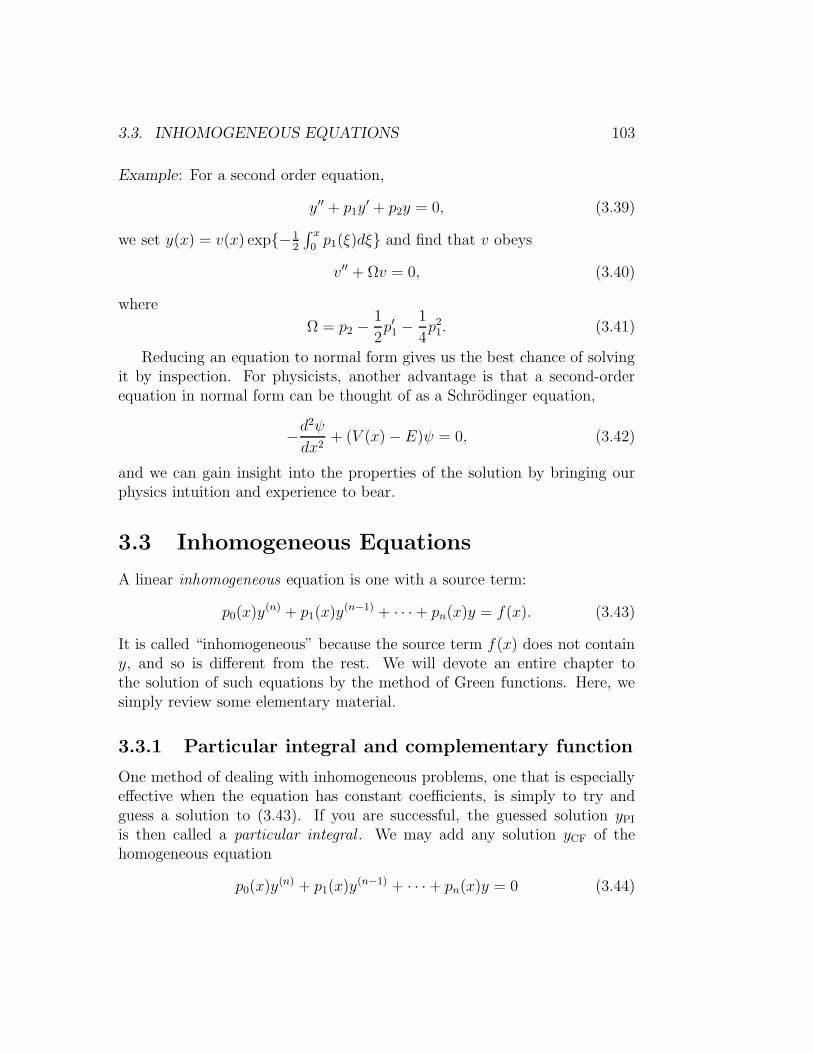
3.3. INHOMOGENEOUS EQUATIONS 103
Example: For a second order equation,
y′′ + p1y′ + p2y = 0, (3.39)
we set y(x) = v(x) exp−12
∫ x0p1(ξ)dξ and find that v obeys
v′′ + Ωv = 0, (3.40)
where
Ω = p2 −1
2p′1 −
1
4p21. (3.41)
Reducing an equation to normal form gives us the best chance of solvingit by inspection. For physicists, another advantage is that a second-orderequation in normal form can be thought of as a Schrodinger equation,
−d2ψ
dx2+ (V (x)−E)ψ = 0, (3.42)
and we can gain insight into the properties of the solution by bringing ourphysics intuition and experience to bear.
3.3 Inhomogeneous Equations
A linear inhomogeneous equation is one with a source term:
p0(x)y(n) + p1(x)y
(n−1) + · · ·+ pn(x)y = f(x). (3.43)
It is called “inhomogeneous” because the source term f(x) does not containy, and so is different from the rest. We will devote an entire chapter tothe solution of such equations by the method of Green functions. Here, wesimply review some elementary material.
3.3.1 Particular integral and complementary function
One method of dealing with inhomogeneous problems, one that is especiallyeffective when the equation has constant coefficients, is simply to try andguess a solution to (3.43). If you are successful, the guessed solution yPIis then called a particular integral . We may add any solution yCF of thehomogeneous equation
p0(x)y(n) + p1(x)y
(n−1) + · · ·+ pn(x)y = 0 (3.44)
104 CHAPTER 3. LINEAR ORDINARY DIFFERENTIAL EQUATIONS
to yPI and it will still be a solution of the inhomogeneous problem. Weuse this freedom to satisfy the boundary or initial conditions. The addedsolution, yCF, is called the complementary function.Example: Charging capacitor. The capacitor in the circuit in figure 3.1 isinitially uncharged. The switch is closed at t = 0
R
CQV
Figure 3.1: Capacitor circuit
The charge on the capacitor, Q, obeys
RdQ
dt+Q
C= V, (3.45)
where R, C, V are constants. A particular integral is given by Q(t) = CV .The complementary-function solution of the homogeneous problem is
Q(t) = Q0e−t/RC , (3.46)
where Q0 is constant. The solution satisfying the initial conditions is
Q(t) = CV(1− e−t/RC
). (3.47)
3.3.2 Variation of parameters
We now follow Lagrange, and solve
p0(x)y(n) + p1(x)y
(n−1) + · · ·+ pn(x)y = f(x) (3.48)
by writingy = v1y1 + v2y2 + · · ·+ vnyn (3.49)
where the yi are the n linearly independent solutions of the homogeneousequation and the vi are functions of x that we have to determine. Thismethod is called variation of parameters .

3.3. INHOMOGENEOUS EQUATIONS 105
Now, differentiating gives
y′ = v1y′1 + v2y
′2 + · · ·+ vny
′n + v′1y1 + v′2y2 + · · ·+ v′nyn . (3.50)
We will chose the v’s so as to make the terms in the braces vanish. Differen-tiate again:
y′′ = v1y′′1 + v2y
′′2 + · · ·+ vny
′′n + v′1y′1 + v′2y
′2 + · · ·+ v′ny
′n . (3.51)
Again, we will chose the v’s to make the terms in the braces vanish. Weproceed in this way until the very last step, at which we demand
v′1y
(n−1)1 + v′2y
(n−1)2 + · · ·+ v′ny
n−1n
= f(x)/p0(x). (3.52)
If you substitute the resulting y into the differential equation, you will seethat the equation is satisfied.
We have imposed the following conditions on v′i:
v′1y1 + v′2y2 + · · ·+ v′nyn = 0,
v′1y′1 + v′2y
′2 + · · ·+ v′ny
′n = 0,
...
v′1y(n−1)1 + v′2y
(n−1)2 + · · ·+ v′ny
n−1n = f(x)/p0(x). (3.53)
This system of linear equations will have a solution for v′1, . . . , v′n, provided
the Wronskian of the yi is non-zero. This, however, is guaranteed by theassumed linear independence of the yi. Having found the v′1, . . . , v
′n, we obtain
the v1, . . . , vn themselves by a single integration.Example: First-order linear equation. A simple and useful application of thismethod solves
dy
dx+ P (x)y = f(x). (3.54)
The solution to the homogeneous equation is
y1 = e−∫ xaP (s) ds. (3.55)
We therefore sety = v(x)e−
∫ xa P (s) ds, (3.56)
and find thatv′(x)e−
∫ xaP (s) ds = f(x). (3.57)

106 CHAPTER 3. LINEAR ORDINARY DIFFERENTIAL EQUATIONS
We integrate once to find
v(x) =
∫ x
b
f(ξ)e∫ ξaP (s) dsdξ, (3.58)
and so
y(x) =
∫ x
b
f(ξ)e−
∫ xξ P (s) ds
dξ. (3.59)
We select b to satisfy the initial condition.
3.4 Singular Points
So far in this chapter, we have been assuming, either explicitly or tacitly, thatour coefficients pi(x) are smooth, and that p0(x) never vanishes. If p0(x) doesbecome zero (or, more precisely, if one or more of the pi/p0 becomes singular)then dramatic things happen, and the location of the zero of p0 is called asingular point of the differential equation. All other points are called ordinarypoints .
In physics application we often find singular points at the ends of theinterval in which we wish to solve our differential equation. For example, theorigin r = 0 is often a singular point when r is the radial coordinate in planeor spherical polars. The existence and uniqueness theorems that we haverelied out throughout this chapter may fail at singular endpoints. Consider,for example, the equation
xy′′ + y′ = 0, (3.60)
which is singular at x = 0. The two linearly independent solutions for x > 0are y1(x) = 1 and y2(x) = ln x. The general solution is therefore A +B ln x,but no choice of A and B can satisfy the initial conditions y(0) = a, y′(0) = bwhen b is non-zero. Because of these complications, we will delay a systematicstudy of singular endpoints until chapter 8.
3.4.1 Regular singular points
If, in the differential equation
p0y′′ + p1y
′ + p2y = 0, (3.61)

3.4. SINGULAR POINTS 107
we have a point x = a such that
p0(x) = (x− a)2P (x), p1(x) = (x− a)Q(x), p2(x) = R(x), (3.62)
where P andQ and R are analytic1 and P andQ non-zero in a neighbourhoodof a then the point x = a is called a regular singular point of the equation.All other singular points are said to be irregular . Close to a regular singularpoint a the equation looks like
P (a)(x− a)2y′′ +Q(a)(x− a)y′ +R(a)y = 0. (3.63)
The solutions of this reduced equation are
y1 = (x− a)λ1 , y2 = (x− a)λ2 , (3.64)
where λ1,2 are the roots of the indicial equation
λ(λ− 1)P (a) + λQ(a) +R(a) = 0. (3.65)
The solutions of the full equation are then
y1 = (x− a)λ1f1(x), y2 = (x− a)λ2f2(x), (3.66)
where f1,2 have power series solutions convergent in a neighbourhood of a.An exception occurs when λ1 and λ2 coincide or differ by an integer, in whichcase the second solution is of the form
y2 = (x− a)λ1(ln(x− a)f1(x) + f2(x)
), (3.67)
where f1 is the same power series that occurs in the first solution, and f2 isa new power series. You will probably have seen these statements proved bythe tedious procedure of setting
f1(x) = (x− a)λ(b0 + b1(x− a) + b2(x− a)2 + · · · , (3.68)
and obtaining a recurrence relation determining the bi. Far more insight isobtained, however, by extending the equation and its solution to the com-plex plane, where the structure of the solution is related to its monodromyproperties. If you are familiar with complex analytic methods, you might liketo look ahead to the discussion of monodromy in section 19.2.
1A function is analytic at a point if it has a power-series expansion that converges tothe function in a neighbourhood of the point.

108 CHAPTER 3. LINEAR ORDINARY DIFFERENTIAL EQUATIONS
3.5 Further Exercises and Problems
Exercise 3.1: Reduction of Order. Sometimes additional information aboutthe solutions of a differential equation enables us to reduce the order of theequation, and so solve it.
a) Suppose that we know that y1 = u(x) is one solution to the equation
y′′ + V (x)y = 0.
By trying y = u(x)v(x) show that
y2 = u(x)
∫ x dξ
u2(ξ)
is also a solution of the differential equation. Is this new solution evermerely a constant mutiple of the old solution, or must it be linearlyindependent? (Hint: evaluate the Wronskian W (y2, y1).)
b) Suppose that we are told that the product, y1y2, of the two solutions tothe equation y′′ + p1y
′ + p2y = 0 is a constant. Show that this requires2p1p2 + p′2 = 0.
c) By using ideas from part b) or otherwise, find the general solution of theequation
(x+ 1)x2y′′ + xy′ − (x+ 1)3y = 0.
Exercise 3.2: Show that the general solution of the differential equation
d2y
dx2− 2
dy
dx+ y =
ex
1 + x2
isy(x) = Aex +Bxex − 1
2ex ln(1 + x2) + xex tan−1x.
Exercise 3.3: Use the method of variation of parameters to show that if y1(x)and y2(x) are linearly independent solutions to the equation
p0(x)d2y
dx2+ p1(x)
dy
dx+ p2(x)y = 0,
then general solution of the equation
p0(x)d2y
dx2+ p1(x)
dy
dx+ p2(x)y = f(x)
is
y(x) = Ay1(x)+By2(x)− y1(x)∫ x y2(ξ)f(ξ)
p0W (y1, y2)dξ+ y2(x)
∫ x y1(ξ)f(ξ)
p0W (y1, y2)dξ.

3.5. FURTHER EXERCISES AND PROBLEMS 109
Problem 3.4: One-dimensional scattering theory. Consider the one-dimensionalSchrodinger equation
−d2ψ
dx2+ V (x)ψ = Eψ,
where V (x) is zero except in a finite interval [−a, a] near the origin.
x
V(x)
a
L R
−a
Figure 3.2: A typical potential V for exercise 3.4
Let L denote the left asymptotic region, −∞ < x < −a, and similarly let Rdenote a < x <∞. For E = k2 there will be scattering solutions of the form
ψk(x) =
eikx + rL(k)e
−ikx, x ∈ L,tL(k)e
ikx, x ∈ R,
which for k > 0 describe waves incident on the potential V (x) from the left.There will be solutions with
ψk(x) =
tR(k)e
ikx, x ∈ L,eikx + rR(k)e
−ikx, x ∈ R,
which for k < 0 describe waves incident from the right. The wavefunctionsin [−a, a] will naturally be more complicated. Observe that [ψk(x)]
∗ is also asolution of the Schrodinger equation.
By using properties of the Wronskian, show that:
a) |rL,R|2 + |tL,R|2 = 1,b) tL(k)=tR(−k).c) Deduce from parts a) and b) that |rL(k)| = |rR(−k)|.d) Take the specific example of V (x) = λδ(x−b) with |b| < a. Compute the
transmission and reflection coefficients and hence show that rL(k) andrR(−k) may differ in phase.

110 CHAPTER 3. LINEAR ORDINARY DIFFERENTIAL EQUATIONS
Exercise 3.5: Suppose ψ(x) obeys a Schrodinger equation
(−1
2
d2
dx2+ [V (x)− E]
)ψ = 0.
a) Make a smooth and invertable change of independent variable by settingx = x(z) and find the second order differential equation in z obeyed byψ(z) ≡ ψ(x(z)). Reduce this equation to normal form, and show thatthe resulting equation is
(−1
2
d2
dz2+ (x′)2[V (x(z))− E]− 1
4x, z
)ψ(z) = 0,
where the primes denote differentiation with respect to z, and
x, z def=
x′′′
x′− 3
2
(x′′
x′
)2
is called the Schwarzian derivative of x with respect to z. Schwarzianderivatives play an important role in conformal field theory and stringtheory.
b) Make a sequence of changes of variable x → z → w, and so establishCayley’s identity
(dz
dw
)2
x, z + z, w = x,w.
(Hint: If your proof takes more than one line, you are missing the point.)

Chapter 4
Linear Differential Operators
In this chapter we will begin to take a more sophisticated approach to dif-ferential equations. We will define, with some care, the notion of a lineardifferential operator, and explore the analogy between such operators andmatrices. In particular, we will investigate what is required for a linear dif-ferential operator to have a complete set of eigenfunctions.
4.1 Formal vs. Concrete Operators
We will call the object
L = p0(x)dn
dxn+ p1(x)
dn−1
dxn−1+ · · ·+ pn(x), (4.1)
which we also write as
p0(x)∂nx + p1(x)∂
n−1x + · · ·+ pn(x), (4.2)
a formal linear differential operator . The word “formal” refers to the factthat we are not yet worrying about what sort of functions the operator isapplied to.
4.1.1 The algebra of formal operators
Even though they are not acting on anything in particular, we can still formproducts of operators. For example if v and w are smooth functions of x wecan define the operators ∂x + v(x) and ∂x + w(x) and find
(∂x + v)(∂x + w) = ∂2x + w′ + (w + v)∂x + vw, (4.3)
111

112 CHAPTER 4. LINEAR DIFFERENTIAL OPERATORS
or(∂x + w)(∂x + v) = ∂2x + v′ + (w + v)∂x + vw, (4.4)
We see from this example that the operator algebra is not usually commuta-tive.
The algebra of formal operators has some deep applications. Consider,for example, the operators
L = −∂2x + q(x) (4.5)
andP = ∂3x + a(x)∂x + ∂xa(x). (4.6)
In the last expression, the combination ∂xa(x) means “first multiply by a(x),and then differentiate the result,” so we could also write
∂xa = a∂x + a′. (4.7)
We can now form the commutator [P, L] ≡ PL − LP . After a little effort,we find
[P, L] = (3q′ + 4a′)∂2x + (3q′′ + 4a′′)∂x + q′′′ + 2aq′ + a′′′. (4.8)
If we choose a = −34q, the commutator becomes a pure multiplication oper-
ator, with no differential part:
[P, L] =1
4q′′′ − 3
2qq′. (4.9)
The equationdL
dt= [P, L], (4.10)
or, equivalently,
q =1
4q′′′ − 3
2qq′, (4.11)
has a formal solutionL(t) = U(t)L(0)U−1(t), (4.12)
where dU/dt = P (t)U(t). This shows that the time evolution of L is givenby a similarity transformation, which (again formally) does not change itseigenvalues. The partial differential equation (4.11) is the famous Kortewegde Vries (KdV) equation, which has “soliton” solutions whose existence isintimately connected with the fact that it can be written as (4.10). Theoperators P and L are called a Lax pair , after Peter Lax who uncoveredmuch of the structure.

4.1. FORMAL VS. CONCRETE OPERATORS 113
4.1.2 Concrete operators
We want to explore the analogies between linear differential operators andmatrices acting on a finite-dimensional vector space. Because the theory ofmatrix operators makes much use of inner products and orthogonality, theanalogy is closest if we work with a function space equipped with these samenotions. We therefore let our differential operators act on L2[a, b], the Hilbertspace of square-integrable functions on [a, b]. Now a differential operatorcannot act on every function in the Hilbert space because not all of themare differentiable. Even though we will relax our notion of differentiabilityand permit weak derivatives, we must at least demand that the domain D,the subset of functions on which we allow the operator to act, contain onlyfunctions that are sufficiently differentiable that the function resulting fromapplying the operator remains an element of L2[a, b]. We will usually restrictthe set of functions even further, by imposing boundary conditions at theendpoints of the interval. A linear differential operator is now defined as aformal linear differential operator, together with a specification of its domainD.
The boundary conditions that we will impose will always be linear andhomogeneous . This is so that the domain of definition is a vector space.In other words, if y1 and y2 obey the boundary conditions then so shouldλy1 + µy2. Thus, for a second-order operator
L = p0∂2x + p1∂x + p2 (4.13)
on the interval [a, b], we might impose
B1[y] = α11y(a) + α12y′(a) + β11y(b) + β12y
′(b) = 0,
B2[y] = α21y(a) + α22y′(a) + β21y(b) + β22y
′(b) = 0, (4.14)
but we will not, in defining the differential operator , impose inhomogeneousconditions, such as
B1[y] = α11y(a) + α12y′(a) + β11y(b) + β12y
′(b) = A,
B2[y] = α21y(a) + α22y′(a) + β21y(b) + β22y
′(b) = B, (4.15)
with non-zero A,B — even though we will solve differential equations withsuch boundary conditions.

114 CHAPTER 4. LINEAR DIFFERENTIAL OPERATORS
Also, for an n-th order operator, we will not constrain derivatives of orderhigher than n−1. This is reasonable1: If we seek solutions of Ly = f with La second-order operator, for example, then the values of y′′ at the endpointsare already determined in terms of y′ and y by the differential equation. Wecannot choose to impose some other value. By differentiating the equationenough times, we can similarly determine all higher endpoint derivatives interms of y and y′. These two derivatives, therefore, are all we can fix by fiat.
The boundary and differentiability conditions that we impose make D asubset of the entire Hilbert space. This subset will always be dense: anyelement of the Hilbert space can be obtained as an L2 limit of functions inD. In particular, there will never be a function in L2[a, b] that is orthogonalto all functions in D.
4.2 The Adjoint Operator
One of the important properties of matrices, established in the appendix,is that a matrix that is self-adjoint, or Hermitian, may be diagonalized . Inother words, the matrix has sufficiently many eigenvectors for them to forma basis for the space on which it acts. A similar property holds for self-adjoint differential operators, but we must be careful in our definition ofself-adjointness.
Before reading this section, We suggest you review the material on adjointoperators on finite-dimensional spaces that appears in the appendix.
4.2.1 The formal adjoint
Given a formal differential operator
L = p0(x)dn
dxn+ p1(x)
dn−1
dxn−1+ · · ·+ pn(x), (4.16)
and a weight function w(x), real and positive on the interval (a, b), we canfind another such operator L†, such that, for any sufficiently differentiableu(x) and v(x), we have
w(u∗Lv − v(L†u)∗
)=
d
dxQ[u, v], (4.17)
1There is a deeper reason which we will explain in section 9.7.2.

4.2. THE ADJOINT OPERATOR 115
for some function Q, which depends bilinearly on u and v and their first n−1derivatives. We call L† the formal adjoint of L with respect to the weight w.The equation (4.17) is called Lagrange’s identity. The reason for the name“adjoint” is that if we define an inner product
〈u, v〉w =
∫ b
a
wu∗v dx, (4.18)
and if the functions u and v have boundary conditions that make Q[u, v]|ba =0, then
〈u, Lv〉w = 〈L†u, v〉w, (4.19)
which is the defining property of the adjoint operator on a vector space. Theword “formal” means, as before, that we are not yet specifying the domainof the operator.
The method for finding the formal adjoint is straightforward: integrateby parts enough times to get all the derivatives off v and on to u.Example: If
L = −i ddx
(4.20)
then let us find the adjoint L† with respect to the weight w ≡ 1. We startfrom
u∗(Lv) = u∗(−i ddxv
),
and use the integration-by-parts technique once to get the derivative off vand onto u∗:
u∗(−i ddxv
)=
(id
dxu∗)v − i d
dx(u∗v)
=
(−i ddxu
)∗v − i d
dx(u∗v)
≡ v(L†u)∗ +d
dxQ[u, v]. (4.21)
We have ended up with the Lagrange identity
u∗(−i ddxv
)− v
(−i ddxu
)∗=
d
dx(−iu∗v), (4.22)

116 CHAPTER 4. LINEAR DIFFERENTIAL OPERATORS
and found that
L† = −i ddx, Q[u, v] = −iu∗v. (4.23)
The operator −id/dx (which you should recognize as the “momentum” op-erator from quantum mechanics) obeys L = L†, and is therefore, formallyself-adjoint , or Hermitian.Example: Let
L = p0d2
dx2+ p1
d
dx+ p2, (4.24)
with the pi all real. Again let us find the adjoint L† with respect to the innerproduct with w ≡ 1. Now, proceeding as above, but integrating by partstwice, we find
u∗ [p0v′′ + p1v
′ + p2v]− v [(p0u)′′ − (p1u)′ + p2u]
∗
=d
dx
[p0(u
∗v′ − vu∗′) + (p1 − p′0)u∗v]. (4.25)
From this we read off that
L† =d2
dx2p0 −
d
dxp1 + p2
= p0d2
dx2+ (2p′0 − p1)
d
dx+ (p′′0 − p′1 + p2). (4.26)
What conditions do we need to impose on p0,1,2 for this L to be formallyself-adjoint with respect to the inner product with w ≡ 1? For L = L† weneed
p0 = p0
2p′0 − p1 = p1 ⇒ p′0 = p1
p′′0 − p′1 + p2 = p2 ⇒ p′′0 = p′1. (4.27)
We therefore require that p1 = p′0, and so
L =d
dx
(p0d
dx
)+ p2, (4.28)
which we recognize as a Sturm-Liouville operator.Example: Reduction to Sturm-Liouville form. Another way to make theoperator
L = p0d2
dx2+ p1
d
dx+ p2, (4.29)

4.2. THE ADJOINT OPERATOR 117
self-adjoint is by a suitable choice of weight function w. Suppose that p0 ispositive on the interval (a, b), and that p0, p1, p2 are all real. Then we maydefine
w =1
p0exp
∫ x
a
(p1p0
)dx′
(4.30)
and observe that it is positive on (a, b), and that
Ly =1
w(wp0y
′)′ + p2y. (4.31)
Now
〈u, Lv〉w − 〈Lu, v〉w = [wp0(u∗v′ − u∗′v)]ba, (4.32)
where
〈u, v〉w =
∫ b
a
wu∗v dx. (4.33)
Thus, provided p0 does not vanish, there is always some inner product withrespect to which a real second-order differential operator is formally self-adjoint.
Note that with
Ly =1
w(wp0y
′)′ + p2y, (4.34)
the eigenvalue equation
Ly = λy (4.35)
can be written
(wp0y′)′ + p2wy = λwy. (4.36)
When you come across a differential equation where, in the term containingthe eigenvalue λ, the eigenfunction is being multiplied by some other function,you should immediately suspect that the operator will turn out to be self-adjoint with respect to the inner product having this other function as itsweight.Illustration (Bargmann-Fock space): This is a more exotic example of aformal adjoint. You may have met with it in quantum mechanics. Considerthe space of polynomials P (z) in the complex variable z = x+ iy. Define aninner product by
〈P,Q〉 = 1
π
∫d2z e−z
∗z [P (z)]∗Q(z),

118 CHAPTER 4. LINEAR DIFFERENTIAL OPERATORS
where d2z ≡ dx dy and the integration is over the entire x, y plane. Withthis inner product, we have
〈zn, zm〉 = n!δnm.
If we define
a =d
dz,
then
〈P, aQ〉 =1
π
∫d2z e−z
∗z [P (z)]∗d
dzQ(z)
= −1
π
∫d2z
(d
dze−z
∗z [P (z)]∗)Q(z)
=1
π
∫d2z e−z
∗zz∗ [P (z)]∗Q(z)
=1
π
∫d2z e−z
∗z [zP (z)]∗Q(z)
= 〈a†P, Q〉
where a† = z, i.e. the operation of multiplication by z. In this case, theadjoint is not even a differential operator.2
Exercise 4.1: Consider the differential operator L = id/dx. Find the formaladjoint of L with respect to the inner product 〈u, v〉w =
∫wu∗v dx, and find
the corresponding surface term Q[u, v].
2In deriving this result we have used the Wirtinger calculus where z and z∗ are treatedas independent variables so that
d
dze−z∗z = −z∗e−z∗z,
and observed that, because [P (z)]∗is a function of z∗ only,
d
dz[P (z)]
∗= 0.
If you are uneasy at regarding z, z∗, as independent, you should confirm these formulaeby expressing z and z∗ in terms of x and y, and using
d
dz≡ 1
2
(∂
∂x− i ∂
∂y
),
d
dz∗≡ 1
2
(∂
∂x+ i
∂
∂y
).

4.2. THE ADJOINT OPERATOR 119
Exercise 4.2:Sturm-Liouville forms. By constructing appropriate weight func-tions w(x) convert the following common operators into Sturm-Liouville form:
a) L = (1− x2) d2/dx2 + [(µ− ν)− (µ + ν + 2)x] d/dx.b) L = (1− x2) d2/dx2 − 3x d/dx.c) L = d2/dx2 − 2x(1− x2)−1 d/dx −m2 (1− x2)−1.
4.2.2 A simple eigenvalue problem
A finite Hermitian matrix has a complete set of orthonormal eigenvectors.Does the same property hold for a Hermitian differential operator?
Consider the differential operator
T = −∂2x, D(T ) = y, Ty ∈ L2[0, 1] : y(0) = y(1) = 0. (4.37)
With the inner product
〈y1, y2〉 =∫ 1
0
y∗1y2 dx (4.38)
we have
〈y1, T y2〉 − 〈Ty1, y2〉 = [y′1∗y2 − y∗1y′2]10 = 0. (4.39)
The integrated-out part is zero because both y1 and y2 satisfy the boundaryconditions. We see that
〈y1, T y2〉 = 〈Ty1, y2〉 (4.40)
and so T is Hermitian or symmetric.The eigenfunctions and eigenvalues of T are
yn(x) = sin nπxλn = n2π2
n = 1, 2, . . . . (4.41)
We see that:i) the eigenvalues are real ;ii) the eigenfunctions for different λn are orthogonal ,
2
∫ 1
0
sin nπx sinmπxdx = δnm, n = 1, 2, . . . (4.42)

120 CHAPTER 4. LINEAR DIFFERENTIAL OPERATORS
iii) the normalized eigenfunctions ϕn(x) =√2 sin nπx are complete: any
function in L2[0, 1] has an (L2) convergent expansion as
y(x) =
∞∑
n=1
an√2 sinnπx (4.43)
where
an =
∫ 1
0
y(x)√2 sin nπx dx. (4.44)
This all looks very good — exactly the properties we expect for finite Her-mitian matrices. Can we carry over all the results of finite matrix theory tothese Hermitian operators? The answer sadly is no! Here is a counterexam-ple:
Let
T = −i∂x, D(T ) = y, Ty ∈ L2[0, 1] : y(0) = y(1) = 0. (4.45)
Again
〈y1, T y2〉 − 〈Ty1, y2〉 =
∫ 1
0
dx y∗1(−i∂xy2)− (−i∂xy1)∗y2
= −i[y∗1y2]10 = 0. (4.46)
Once more, the integrated out part vanishes due to the boundary conditionssatisfied by y1 and y2, so T is nicely Hermitian. Unfortunately, T with theseboundary conditions has no eigenfunctions at all — never mind a completeset! Any function satisfying Ty = λy will be proportional to eiλx, but an ex-ponential function is never zero, and cannot satisfy the boundary conditions.
It seems clear that the boundary conditions are the problem. We needa better definition of “adjoint” than the formal one — one that pays moreattention to boundary conditions. We will then be forced to distinguishbetween mere Hermiticity, or symmetry , and true self-adjointness.
Exercise 4.3: Another disconcerting example. Let p = −i∂x. Show that thefollowing operator on the infinite real line is formally self-adjoint:
H = x3p+ px3. (4.47)
Now let
ψλ(x) = |x|−3/2 exp
− λ
4x2
, (4.48)
4.2. THE ADJOINT OPERATOR 121
where λ is real and positive. Show that
Hψλ = −iλψλ, (4.49)
so ψλ is an eigenfunction with a purely imaginary eigenvalue. Examine theproof that Hermitian operators have real eigenvalues, and identify at whichpoint it fails. (Hint: H is formally self adjoint because it is of the form T +T †.Now ψλ is square-integrable, and so an element of L2(R). Is Tψλ an elementof L2(R)?)
4.2.3 Adjoint boundary conditions
The usual definition of the adjoint operator in linear algebra is as follows:Given the operator T : V → V and an inner product 〈 , 〉, we look at〈u, Tv〉, and ask if there is a w such that 〈w, v〉 = 〈u, Tv〉 for all v. If thereis, then u is in the domain of T †, and we set T †u = w.
For finite-dimensional vector spaces V there always is such a w, and sothe domain of T † is the entire space. In an infinite dimensional Hilbert space,however, not all 〈u, Tv〉 can be written as 〈w, v〉with w a finite-length elementof L2. In particular δ-functions are not allowed — but these are exactly whatwe would need if we were to express the boundary values appearing in theintegrated out part, Q(u, v), as an inner-product integral. We must thereforeensure that u is such that Q(u, v) vanishes, but then accept any u with thisproperty into the domain of T †. What this means in practice is that we lookat the integrated out term Q(u, v) and see what is required of u to makeQ(u, v) zero for any v satisfying the boundary conditions appearing in D(T ).These conditions on u are the adjoint boundary conditions , and define thedomain of T †.Example: Consider
T = −i∂x, D(T ) = y, Ty ∈ L2[0, 1] : y(1) = 0. (4.50)
Now,
∫ 1
0
dx u∗(−i∂xv) = −i[u∗(1)v(1)− u∗(0)v(0)] +∫ 1
0
dx(−i∂xu)∗v
= −i[u∗(1)v(1)− u∗(0)v(0)] + 〈w, v〉, (4.51)
where w = −i∂xu. Since v(x) is in the domain of T , we have v(1) = 0, andso the first term in the integrated out bit vanishes whatever value we take

122 CHAPTER 4. LINEAR DIFFERENTIAL OPERATORS
for u(1). On the other hand, v(0) could be anything, so to be sure that thesecond term vanishes we must demand that u(0) = 0. This, then, is theadjoint boundary condition. It defines the domain of T †:
T † = −i∂x, D(T †) = y, Ty ∈ L2[0, 1] : y(0) = 0. (4.52)
For our problematic operator
T = −i∂x, D(T ) = y, Ty ∈ L2[0, 1] : y(0) = y(1) = 0, (4.53)
we have∫ 1
0
dx u∗(−i∂xv) = −i[u∗v]10 +∫ 1
0
dx(−i∂xu)∗v
= 0 + 〈w, v〉, (4.54)
where again w = −i∂xu. This time no boundary conditions need be imposedon u to make the integrated out part vanish. Thus
T † = −i∂x, D(T †) = y, Ty ∈ L2[0, 1]. (4.55)
Although any of these operators “T = −i∂x” is formally self-adjoint wehave,
D(T ) 6= D(T †), (4.56)
so T and T † are not the same operator and none of them is truly self-adjoint.
Exercise 4.4: Consider the differential operator M = d4/dx4, Find the formaladjoint of M with respect to the inner product 〈u, v〉 =
∫u∗v dx, and find
the corresponding surface term Q[u, v]. Find the adjoint boundary conditionsdefining the domain of M † for the case
D(M) = y, y(4) ∈ L2[0, 1] : y(0) = y′′′(0) = y(1) = y′′′(1) = 0.
4.2.4 Self-adjoint boundary conditions
A formally self-adjoint operator T is truly self adjoint only if the domains ofT † and T coincide. From now on, the unqualified phrase “self-adjoint” willalways mean “truly self-adjoint.”
Self-adjointness is usually desirable in physics problems. It is thereforeuseful to investigate what boundary conditions lead to self-adjoint operators.
4.2. THE ADJOINT OPERATOR 123
For example, what are the most general boundary conditions we can imposeon T = −i∂x if we require the resultant operator to be self-adjoint? Now,
∫ 1
0
dx u∗(−i∂xv)−∫ 1
0
dx(−i∂xu)∗v = −i(u∗(1)v(1)− u∗(0)v(0)
). (4.57)
Demanding that the right-hand side be zero gives us, after division by u∗(0)v(1),
u∗(1)
u∗(0)=v(0)
v(1). (4.58)
We require this to be true for any u and v obeying the same boundaryconditions. Since u and v are unrelated, both sides must equal a constant κ,and furthermore this constant must obey κ∗ = κ−1 in order that u(1)/u(0)be equal to v(1)/v(0). Thus, the boundary condition is
u(1)
u(0)=v(1)
v(0)= eiθ (4.59)
for some real angle θ. The domain is therefore
D(T ) = y, Ty ∈ L2[0, 1] : y(1) = eiθy(0). (4.60)
These are twisted periodic boundary conditions.With these generalized periodic boundary conditions, everything we ex-
pect of a self-adjoint operator actually works:i) The functions un = ei(2πn+θ)x, with n = . . . ,−2,−1, 0, 1, 2 . . . are eigen-
functions of T with eigenvalues kn ≡ 2πn+ θ.ii) The eigenvalues are real.iii) The eigenfunctions form a complete orthonormal set.
Because self-adjoint operators possess a complete set of mutually orthogo-nal eigenfunctions, they are compatible with the interpretational postulatesof quantum mechanics, where the square of the inner product of a statevector with an eigenstate gives the probability of measuring the associatedeigenvalue. In quantum mechanics, self-adjoint operators are therefore calledobservables .Example: The Sturm-Liouville equation. With
L =d
dxp(x)
d
dx+ q(x), x ∈ [a, b], (4.61)

124 CHAPTER 4. LINEAR DIFFERENTIAL OPERATORS
we have
〈u, Lv〉 − 〈Lu, v〉 = [p(u∗v′ − u′∗v)]ba. (4.62)
Let us seek to impose boundary conditions separately at the two ends. Thus,at x = a we want
(u∗v′ − u′∗v)|a = 0, (4.63)
oru′∗(a)
u∗(a)=v′(a)
v(a), (4.64)
and similarly at b. If we want the boundary conditions imposed on v (whichdefine the domain of L) to coincide with those for u (which define the domainof L†) then we must have
v′(a)
v(a)=u′(a)
u(a)= tan θa (4.65)
for some real angle θa, and similar boundary conditions with a θb at b. Wecan also write these boundary conditions as
αay(a) + βay′(a) = 0,
αby(b) + βby′(b) = 0. (4.66)
Deficiency indices and self-adjoint extensions
There is a general theory of self-adjoint boundary conditions, due to Her-mann Weyl and John von Neumann. We will not describe this theory in anydetail, but simply give their recipe for counting the number of parametersin the most general self-adjoint boundary condition: To find this number wedefine an initial domain D0(L) for the operator L by imposing the strictestpossible boundary conditions. This we do by setting to zero the bound-ary values of all the y(n) with n less than the order of the equation. Nextcount the number of square-integrable eigenfunctions of the resulting adjointoperator T † corresponding to eigenvalue ±i. The numbers, n+ and n−, ofthese eigenfunctions are called the deficiency indices . If they are not equalthen there is no possible way to make the operator self-adjoint. If they areequal, n+ = n− = n, then there is an n2 real-parameter family of self-adjointextensions D(L) ⊃ D0(L) of the initial tightly-restricted domain.

4.2. THE ADJOINT OPERATOR 125
Example: The sad case of the “radial momentum operator.” We wish todefine the operator Pr = −i∂r on the half-line 0 < r <∞. We start with therestrictive domain
Pr = −i∂r, D0(T ) = y, Pry ∈ L2[0,∞] : y(0) = 0. (4.67)
We then have
P †r = −i∂r, D(P †
r ) = y, P †r y ∈ L2[0,∞] (4.68)
with no boundary conditions. The equation P †r y = iy has a normalizable
solution y = e−r. The equation P †r y = −iy has no normalizable solution.
The deficiency indices are therefore n+ = 1, n− = 0, and this operatorcannot be rescued and made self adjoint.Example: The Schrodinger operator. We now consider −∂2x on the half-line.Set
T = −∂2x, D0(T ) = y, Ty ∈ L2[0,∞] : y(0) = y′(0) = 0. (4.69)
We then have
T † = −∂2x, D(T †) = y, T †y ∈ L2[0,∞]. (4.70)
Again T † comes with no boundary conditions. The eigenvalue equationT †y = iy has one normalizable solution y(x) = e(i−1)x/
√2, and the equation
T †y = −iy also has one normalizable solution y(x) = e−(i+1)x/√2. The defi-
ciency indices are therefore n+ = n− = 1. The Weyl-von Neumann theorynow says that, by relaxing the restrictive conditions y(0) = y′(0) = 0, wecan extend the domain of definition of the operator to find a one-parameterfamily of self-adjoint boundary conditions. These will be the conditionsy′(0)/y(0) = tan θ that we found above.
If we consider the operator −∂2x on the finite interval [a, b], then bothsolutions of (T † ± i)y = 0 are normalizable, and the deficiency indices willbe n+ = n− = 2. There should therefore be 22 = 4 real parameters in theself-adjoint boundary conditions. This is a larger class than those we foundin (4.66), because it includes generalized boundary conditions of the form
B1[y] = α11y(a) + α12y′(a) + β11y(b) + β12y
′(b) = 0,
B2[y] = α21y(a) + α22y′(a) + β21y(b) + β22y
′(b) = 0
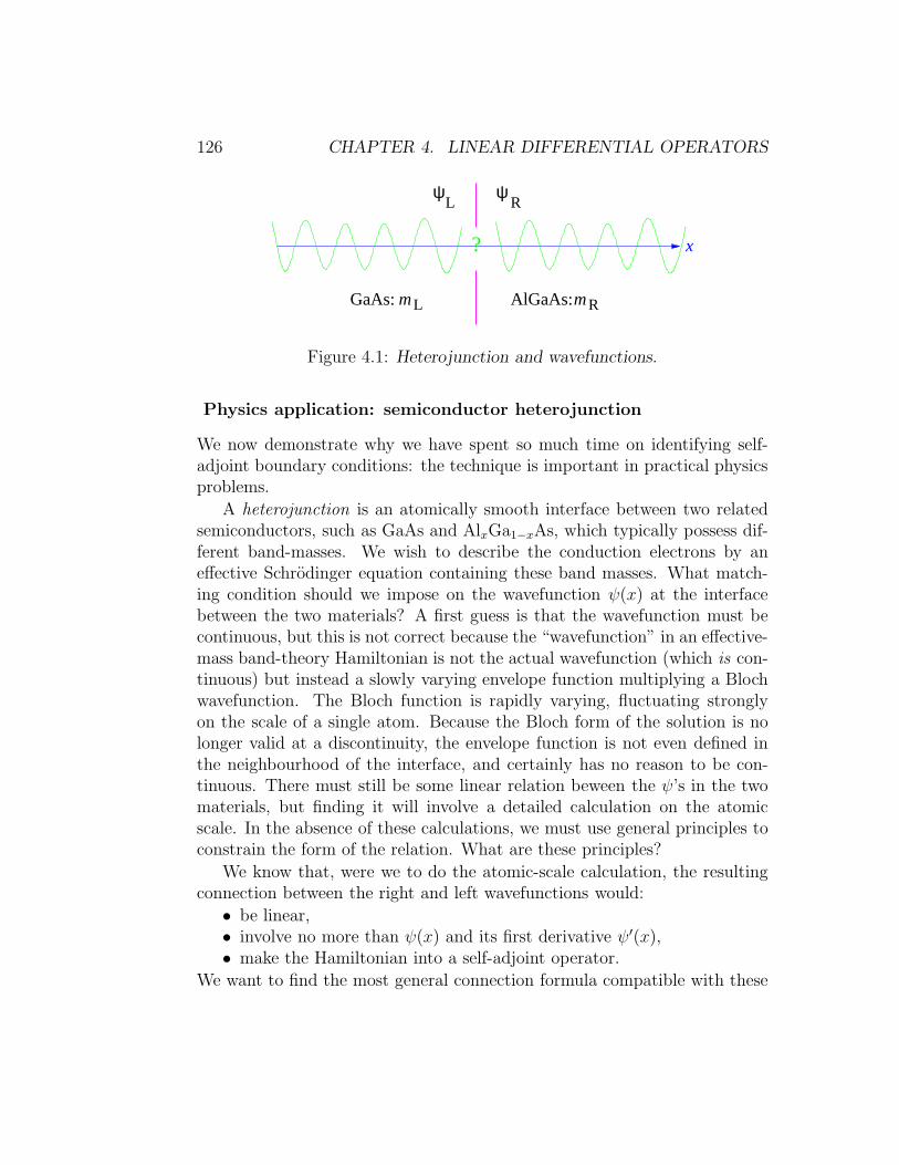
126 CHAPTER 4. LINEAR DIFFERENTIAL OPERATORS
ψ L R
ψ
x?
GaAs:mL AlGaAs:mR
Figure 4.1: Heterojunction and wavefunctions.
Physics application: semiconductor heterojunction
We now demonstrate why we have spent so much time on identifying self-adjoint boundary conditions: the technique is important in practical physicsproblems.
A heterojunction is an atomically smooth interface between two relatedsemiconductors, such as GaAs and AlxGa1−xAs, which typically possess dif-ferent band-masses. We wish to describe the conduction electrons by aneffective Schrodinger equation containing these band masses. What match-ing condition should we impose on the wavefunction ψ(x) at the interfacebetween the two materials? A first guess is that the wavefunction must becontinuous, but this is not correct because the “wavefunction” in an effective-mass band-theory Hamiltonian is not the actual wavefunction (which is con-tinuous) but instead a slowly varying envelope function multiplying a Blochwavefunction. The Bloch function is rapidly varying, fluctuating stronglyon the scale of a single atom. Because the Bloch form of the solution is nolonger valid at a discontinuity, the envelope function is not even defined inthe neighbourhood of the interface, and certainly has no reason to be con-tinuous. There must still be some linear relation beween the ψ’s in the twomaterials, but finding it will involve a detailed calculation on the atomicscale. In the absence of these calculations, we must use general principles toconstrain the form of the relation. What are these principles?
We know that, were we to do the atomic-scale calculation, the resultingconnection between the right and left wavefunctions would:
• be linear,• involve no more than ψ(x) and its first derivative ψ′(x),• make the Hamiltonian into a self-adjoint operator.
We want to find the most general connection formula compatible with these

4.2. THE ADJOINT OPERATOR 127
principles. The first two are easy to satisfy. We therefore investigate whatmatching conditions are compatible with self-adjointness.
Suppose that the band masses are mL and mR, so that
H = − 1
2mL
d2
dx2+ VL(x), x < 0,
= − 1
2mR
d2
dx2+ VR(x), x > 0. (4.71)
Integrating by parts, and keeping the terms at the interface gives us
〈ψ1, Hψ2〉−〈Hψ1, ψ2〉 =1
2mL
ψ∗1Lψ
′2L − ψ′∗
1Lψ2L
− 1
2mR
ψ∗1Rψ
′2R − ψ′∗
1Rψ2R
.
(4.72)Here, ψL,R refers to the boundary values of ψ immediately to the left or rightof the junction, respectively. Now we impose general linear homogeneousboundary conditions on ψ2:
(ψ2L
ψ′2L
)=
(a bc d
)(ψ2R
ψ′2R
). (4.73)
This relation involves four complex, and therefore eight real, parameters.Demanding that
〈ψ1, Hψ2〉 = 〈Hψ1, ψ2〉, (4.74)
we find
1
2mL
ψ∗1L(cψ2R + dψ′
2R)− ψ′∗1L(aψ2R + bψ′
2R)=
1
2mR
ψ∗1Rψ
′2R − ψ′∗
1Rψ2R
,
(4.75)and this must hold for arbitrary ψ2R, ψ
′2R, so, picking off the coefficients of
these expressions and complex conjugating, we find
(ψ1R
ψ′1R
)=
(mR
mL
)(d∗ −b∗−c∗ a∗
)(ψ1L
ψ′1L
). (4.76)
Because we wish the domain of H† to coincide with that of H , these mustbe same conditions that we imposed on ψ2. Thus we must have
(a bc d
)−1
=
(mR
mL
)(d∗ −b∗−c∗ a∗
). (4.77)

128 CHAPTER 4. LINEAR DIFFERENTIAL OPERATORS
Since (a bc d
)−1
=1
ad− bc
(d −b−c a
), (4.78)
we see that this requires(a bc d
)= eiφ
√mL
mR
(A BC D
), (4.79)
where φ, A, B, C, D are real, and AD−BC = 1. Demanding self-adjointnesshas therefore cut the original eight real parameters down to four. Thesecan be determined either by experiment or by performing the microscopiccalculation.3 Note that 4 = 22, a perfect square, as required by the Weyl-Von Neumann theory.
Exercise 4.5: Consider the Schrodinger operator H = −∂2x on the interval[0, 1]. Show that the most general self-adjoint boundary condition applicableto H can be written as
[ϕ(0)ϕ′(0)
]= eiφ
[a bc d
] [ϕ(1)ϕ′(1)
],
where φ, a, b, c, d are real and ad − bc = 1. Consider H as the quantumHamiltonian of a particle on a ring constructed by attaching x = 0 to x = 1.Show that the self-adjoint boundary condition found above leads to unitaryscattering at the point of join. Does the most general unitary point-scatteringmatrix correspond to the most general self-adjoint boundary condition?
4.3 Completeness of Eigenfunctions
Now that we have a clear understanding of what it means to be self-adjoint,we can reiterate the basic claim: an operator T that is self-adjoint withrespect to an L2[a, b] inner product possesses a complete set of mutually or-thogonal eigenfunctions. The proof that the eigenfunctions are orthogonalis identical to that for finite matrices. We will sketch a proof of the com-pleteness of the eigenfunctions of the Sturm-Liouville operator in the nextsection.
The set of eigenvalues is, with some mathematical cavils, called the spec-trum of T . It is usually denoted by σ(T ). An eigenvalue is said to belong to
3For example, see: T. Ando, S. Mori, Surface Science 113 (1982) 124.

4.3. COMPLETENESS OF EIGENFUNCTIONS 129
the point spectrum when its associated eigenfunction is normalizable i.e isa bona-fide member of L2[a, b] having a finite length. Usually (but not al-ways) the eigenvalues of the point spectrum form a discrete set, and so thepoint spectrum is also known as the discrete spectrum. When the opera-tor acts on functions on an infinite interval, the eigenfunctions may fail tobe normalizable. The associated eigenvalues are then said to belong to thecontinuous spectrum. Sometimes, e.g. the hydrogen atom, the spectrum ispartly discrete and partly continuous. There is also something called theresidual spectrum, but this does not occur for self-adjoint operators.
4.3.1 Discrete spectrum
The simplest problems have a purely discrete spectrum. We have eigenfunc-tions φn(x) such that
Tφn(x) = λnφn(x), (4.80)
where n is an integer. After multiplication by suitable constants, the φn areorthonormal, ∫
φ∗n(x)φm(x) dx = δnm, (4.81)
and complete. We can express the completeness condition as the statementthat ∑
n
φn(x)φ∗n(x
′) = δ(x− x′). (4.82)
If we take this representation of the delta function and multiply it by f(x′)and integrate over x′, we find
f(x) =∑
n
φn(x)
∫φ∗n(x
′)f(x′) dx′. (4.83)
So,
f(x) =∑
n
anφn(x) (4.84)
with
an =
∫φ∗n(x
′)f(x′) dx′. (4.85)
This means that if we can expand a delta function in terms of the φn(x), wecan expand any (square integrable) function.

130 CHAPTER 4. LINEAR DIFFERENTIAL OPERATORS
0.2 0.4 0.6 0.8 1
20
40
60
Figure 4.2: The sum∑70
n=1 2 sin(nπx) sin(nπx′) for x′ = 0.4. Take note of
the very disparate scales on the horizontal and vertical axes.
Warning: The convergence of the series∑
n φn(x)φ∗n(x
′) to δ(x − x′) isneither pointwise nor in the L2 sense. The sum tends to a limit only in thesense of a distribution — meaning that we must multiply the partial sums bya smooth test function and integrate over x before we have something thatactually converges in any meaningful manner. As an illustration consider ourfavourite orthonormal set: φn(x) =
√2 sin(nπx) on the interval [0, 1]. A plot
of the first 70 terms in the sum
∞∑
n=1
√2 sin(nπx)
√2 sin(nπx′) = δ(x− x′)
is shown in figure 4.2. The “wiggles” on both sides of the spike at x =x′ do not decrease in amplitude as the number of terms grows. They do,however, become of higher and higher frequency. When multiplied by asmooth function and integrated, the contributions from adjacent positive andnegative wiggle regions tend to cancel, and it is only after this integrationthat the sum tends to zero away from the spike at x = x′.
Rayleigh-Ritz and completeness
For the Schrodinger eigenvalue problem
Ly = −y′′ + q(x)y = λy, x ∈ [a, b], (4.86)

4.3. COMPLETENESS OF EIGENFUNCTIONS 131
the large eigenvalues are λn ≈ n2π2/(a − b)2. This is because the term qyeventually becomes negligeable compared to λy, and we can then solve theequation with sines and cosines. We see that there is no upper limit tothe magnitude of the eigenvalues. The eigenvalues of the Sturm-Liouvilleproblem
Ly = −(py′)′ + qy = λy, x ∈ [a, b], (4.87)
are similarly unbounded. We will use this unboundedness of the spectrum tomake an estimate of the rate of convergence of the eigenfunction expansionfor functions in the domain of L, and extend this result to prove that theeigenfunctions form a complete set.
We know from chapter one that the Sturm-Liouville eigenvalues are thestationary values of 〈y, Ly〉 when the function y is constrained to have unitlength, 〈y, y〉 = 1. The lowest eigenvalue, λ0, is therefore given by
λ0 = infy∈D(L)
〈y, Ly〉〈y, y〉 . (4.88)
As the variational principle, this formula provides a well-known method ofobtaining approximate ground state energies in quantum mechanics. Part ofits effectiveness comes from the stationary nature of 〈y, Ly〉 at the minimum:a crude approximation to y often gives a tolerably good approximation to λ0.In the wider world of eigenvalue problems, the variational principle is namedafter Rayleigh and Ritz.4
Suppose we have already found the first n normalized eigenfunctionsy0, y1, . . . , yn−1. Let the space spanned by these functions be Vn. Then anobvious extension of the variational principle gives
λn = infy∈V ⊥
n
〈y, Ly〉〈y, y〉 . (4.89)
We now exploit this variational estimate to show that if we expand an arbi-trary y in the domain of L in terms of the full set of eigenfunctions ym,
y =∞∑
m=0
amym, (4.90)
4J. W. Strutt (later Lord Rayleigh), “In Finding the Correction for the Open End ofan Organ-Pipe.” Phil. Trans. 161 (1870) 77; W. Ritz, ”Uber eine neue Methode zurLosung gewisser Variationsprobleme der mathematischen Physik.” J. reine angew. Math.135 (1908).

132 CHAPTER 4. LINEAR DIFFERENTIAL OPERATORS
wheream = 〈ym, y〉, (4.91)
then the sum does indeed converge to y.Let
hn = y −n−1∑
m=0
amym (4.92)
be the residual error after the first n terms. By definition, hn ∈ V ⊥n . Let
us assume that we have adjusted, by adding a constant to q if necessary, Lso that all the λm are positive. This adjustment will not affect the ym. Weexpand out
〈hn, Lhn〉 = 〈y, Ly〉 −n−1∑
m=0
λm|am|2, (4.93)
where we have made use of the orthonormality of the ym. The subtractedsum is guaranteed positive, so
〈hn, Lhn〉 ≤ 〈y, Ly〉. (4.94)
Combining this inequality with Rayleigh-Ritz tells us that
〈y, Ly〉〈hn, hn〉
≥ 〈hn, Lhn〉〈hn, hn〉≥ λn. (4.95)
In other words〈y, Ly〉λn
≥ ‖y −n−1∑
m=0
amym‖2. (4.96)
Since 〈y, Ly〉 is independent of n, and λn →∞, we have ‖y −∑n−10 amym‖2 → 0.
Thus the eigenfunction expansion indeed converges to y, and does so fasterthan λ−1
n goes to zero.Our estimate of the rate of convergence applies only to the expansion of
functions y for which 〈y, Ly〉 is defined — i.e. to functions y ∈ D (L). Thedomain D (L) is always a dense subset of the entire Hilbert space L2[a, b],however, and, since a dense subset of a dense subset is also dense in the largerspace, we have shown that the linear span of the eigenfunctions is a densesubset of L2[a, b]. Combining this observation with the alternative definitionof completeness in 2.2.3, we see that the eigenfunctions do indeed form acomplete orthonormal set. Any square integrable function therefore has aconvergent expansion in terms of the ym, but the rate of convergence maywell be slower than that for functions y ∈ D (L).

4.3. COMPLETENESS OF EIGENFUNCTIONS 133
Operator methods
Sometimes there are tricks for solving the eigenvalue problem.Example: Quantum Harmonic Oscillator. Consider the operator
H = (−∂x + x)(∂x + x) + 1 = −∂2x + x2. (4.97)
This is in the form Q†Q + 1, where Q = (∂x + x), and Q† = (−∂x + x) is itsformal adjoint. If we write these operators in the opposite order we have
QQ† = (∂x + x)(−∂x + x) = −∂2x + x2 + 1 = H + 1. (4.98)
Now, if ψ is an eigenfunction of Q†Q with non-zero eigenvalue λ then Qψ iseigenfunction of QQ† with the same eigenvalue. This is because
Q†Qψ = λψ (4.99)
implies thatQ(Q†Qψ) = λQψ, (4.100)
orQQ†(Qψ) = λ(Qψ). (4.101)
The only way that Qψ can fail to be an eigenfunction of QQ† is if it happensthat Qψ = 0, but this implies that Q†Qψ = 0 and so the eigenvalue was zero.Conversely, if the eigenvalue is zero then
0 = 〈ψ,Q†Qψ〉 = 〈Qψ,Qψ〉, (4.102)
and so Qψ = 0. In this way, we see that Q†Q and QQ† have exactly thesame spectrum, with the possible exception of any zero eigenvalue.
Now notice that Q†Q does have a zero eigenvalue because
ψ0 = e−12x2 (4.103)
obeys Qψ0 = 0 and is normalizable. The operator QQ†, considered as anoperator on L2[−∞,∞], does not have a zero eigenvalue because this wouldrequire Q†ψ = 0, and so
ψ = e+12x2, (4.104)
which is not normalizable, and so not an element of L2[−∞,∞].Since
H = Q†Q+ 1 = QQ† − 1, (4.105)

134 CHAPTER 4. LINEAR DIFFERENTIAL OPERATORS
we see that ψ0 is an eigenfunction of H with eigenvalue 1, and so an eigen-function of QQ† with eigenvalue 2. Hence Q†ψ0 is an eigenfunction of Q†Qwith eigenvalue 2 and so an eigenfunction H with eigenvalue 3. Proceedingin the way we find that
ψn = (Q†)nψ0 (4.106)
is an eigenfunction of H with eigenvalue 2n+ 1.Since Q† = −e 1
2x2∂xe
− 12x2 , we can write
ψn(x) = Hn(x)e− 1
2x2 , (4.107)
where
Hn(x) = (−1)nex2 dn
dxne−x
2
(4.108)
are the Hermite Polynomials .This is a useful technique for any second-order operator that can be fac-
torized — and a surprising number of the equations for “special functions”can be. You will see it later, both in the exercises and in connection withBessel functions.
Exercise 4.6: Show that we have found all the eigenfunctions and eigenvaluesof H = −∂2x + x2. Hint: Show that Q lowers the eigenvalue by 2 and use thefact that Q†Q cannot have negative eigenvalues.
Problem 4.7: Schrodinger equations of the form
−d2ψ
dx2− l(l + 1)sech2xψ = Eψ
are known as Poschel-Teller equations. By setting u = ltanhx and followingthe strategy of this problem one may relate solutions for l to those for l−1 andso find all bound states and scattering eigenfunctions for any integer l.
a) Suppose that we know that ψ = exp−∫ x
u(x′)dx′is a solution of
Lψ ≡(− d2
dx2+W (x)
)ψ = 0.
Show that L can be written as L =M †M where
M =
(d
dx+ u(x)
), M † =
(− d
dx+ u(x)
),
the adjoint being taken with respect to the product 〈u, v〉 =∫u∗v dx.

4.3. COMPLETENESS OF EIGENFUNCTIONS 135
b) Now assume L is acting on functions on [−∞,∞] and that we not haveto worry about boundary conditions. Show that given an eigenfunctionψ− obeying M †Mψ− = λψ− we can multiply this equation on the leftby M and so find a eigenfunction ψ+ with the same eigenvalue for thedifferential operator
L′ =MM † =
(d
dx+ u(x)
)(− d
dx+ u(x)
)
and vice-versa. Show that this correspondence ψ− ↔ ψ+ will fail if, andonly if , λ = 0.
c) Apply the strategy from part b) in the case u(x) = tanhx and one of thetwo differential operators M †M , MM † is (up to an additive constant)
H = − d
dx
2
− 2 sech2x.
Show that H has eigenfunctions of the form ψk = eikxP (tanh x) andeigenvalue E = k2 for any k in the range −∞ < k < ∞. The functionP (tanhx) is a polynomial in tanhx which you should be able to findexplicitly. By thinking about the exceptional case λ = 0, show that Hhas an eigenfunction ψ0(x), with eigenvalue E = −1, that tends rapidlyto zero as x→ ±∞. Observe that there is no corresponding eigenfunctionfor the other operator of the pair.
4.3.2 Continuous spectrum
Rather than a give formal discussion, we will illustrate this subject with someexamples drawn from quantum mechanics.
The simplest example is the free particle on the real line. We have
H = −∂2x. (4.109)
We eventually want to apply this to functions on the entire real line, but wewill begin with the interval [−L/2, L/2], and then take the limit L→∞
The operator H has formal eigenfunctions
ϕk(x) = eikx, (4.110)
corresponding to eigenvalues λ = k2. Suppose we impose periodic boundaryconditions at x = ±L/2:
ϕk(−L/2) = ϕk(+L/2). (4.111)

136 CHAPTER 4. LINEAR DIFFERENTIAL OPERATORS
This selects kn = 2πn/L, where n is any positive, negative or zero integer,and allows us to find the normalized eigenfunctions
χn(x) =1√Leiknx. (4.112)
The completeness condition is
∞∑
n=−∞
1
Leiknxe−iknx
′
= δ(x− x′), x, x′ ∈ [−L/2, L/2]. (4.113)
As L becomes large, the eigenvalues become so close that they can hardly bedistinguished; hence the name continuous spectrum,5 and the spectrum σ(H)becomes the entire positive real line. In this limit, the sum on n becomes anintegral
∞∑
n=−∞
. . .
→∫dn
. . .
=
∫dk
(dn
dk
). . .
, (4.114)
wheredn
dk=
L
2π(4.115)
is called the (momentum) density of states. If we divide this by L to get adensity of states per unit length, we get an L independent “finite” quantity,the local density of states . We will often write
dn
dk= ρ(k). (4.116)
If we express the density of states in terms of the eigenvalue λ then, byan abuse of notation, we have
ρ(λ) ≡ dn
dλ=
L
2π√λ. (4.117)
5When L is strictly infinite, ϕk(x) is no longer normalizable. Mathematicians do notallow such un-normalizable functions to be considered as true eigenfunctions, and so apoint in the continuous spectrum is not, to them, actually an eigenvalue. Instead, theysay that a point λ lies in the continuous spectrum if for any ǫ > 0 there exists an ap-proximate eigenfunction ϕǫ such that ‖ϕǫ‖ = 1, but ‖Lϕǫ − λϕǫ‖ < ǫ. This is not aprofitable definition for us. We prefer to regard non-normalizable wavefunctions as beingdistributions in our rigged Hilbert space.

4.3. COMPLETENESS OF EIGENFUNCTIONS 137
Note thatdn
dλ= 2
dn
dk
dk
dλ, (4.118)
which looks a bit weird, but remember that two states, ±kn, correspond tothe same λ and that the symbols
dn
dk,
dn
dλ(4.119)
are ratios of measures, i.e. Radon-Nikodym derivatives , not ordinary deriva-tives.
In the L→∞ limit, the completeness condition becomes
∫ ∞
−∞
dk
2πeik(x−x
′) = δ(x− x′), (4.120)
and the length L has disappeared.
Suppose that we now apply boundary conditions y = 0 on x = ±L/2.The normalized eigenfunctions are then
χn =
√2
Lsin kn(x+ L/2), (4.121)
where kn = nπ/L. We see that the allowed k’s are twice as close together asthey were with periodic boundary conditions, but now n is restricted to beinga positive non-zero integer. The momentum density of states is therefore
ρ(k) =dn
dk=L
π, (4.122)
which is twice as large as in the periodic case, but the eigenvalue density ofstates is
ρ(λ) =L
2π√λ, (4.123)
which is exactly the same as before.
That the number of states per unit energy per unit volume does notdepend on the boundary conditions at infinity makes physical sense: nolocal property of the sublunary realm should depend on what happens inthe sphere of fixed stars. This point was not fully grasped by physicists,

138 CHAPTER 4. LINEAR DIFFERENTIAL OPERATORS
however, until Rudolph Peierls6 explained that the quantum particle had toactually travel to the distant boundary and back before the precise natureof the boundary could be felt. This journey takes time T (depending onthe particle’s energy) and from the energy-time uncertainty principle, wecan distinguish one boundary condition from another only by examining thespectrum with an energy resolution finer than ~/T . Neither the distance northe nature of the boundary can affect the coarse details, such as the localdensity of states.
The dependence of the spectrum of a general differential operator onboundary conditions was investigated by Hermann Weyl. Weyl distinguishedtwo classes of singular boundary points: limit-circle, where the spectrumdepends on the choice of boundary conditions, and limit-point , where it doesnot. For the Schrodinger operator, the point at infinity, which is “singular”simply because it is at infinity, is in the limit-point class. We will discussWeyl’s theory of singular endpoints in chapter 8.
Phase-shifts
Consider the eigenvalue problem(− d2
dr2+ V (r)
)ψ = Eψ (4.124)
on the interval [0, R], and with boundary conditions ψ(0) = 0 = ψ(R). Thisproblem arises when we solve the Schrodinger equation for a central potentialin spherical polar coordinates, and assume that the wavefunction is a functionof r only (i.e. S-wave, or l = 0). Again, we want the boundary at R to beinfinitely far away, but we will start with R at a large but finite distance,and then take the R →∞ limit. Let us first deal with the simple case thatV (r) ≡ 0; then the solutions are
ψk(r) ∝ sin kr, (4.125)
with eigenvalue E = k2, and with the allowed values of being given byknR = nπ. Since ∫ R
0
sin2(knr) dr =R
2, (4.126)
6Peierls proved that the phonon contribution to the specific heat of a crystal could becorrectly calculated by using periodic boundary conditions. Some sceptics had thoughtthat such “unphysical” boundary conditions would give a result wrong by factors of two.

4.3. COMPLETENESS OF EIGENFUNCTIONS 139
the normalized wavefunctions are
ψk =
√2
Rsin kr, (4.127)
and completeness reads∞∑
n=1
(2
R
)sin(knr) sin(knr
′) = δ(r − r′). (4.128)
As R becomes large, this sum goes over to an integral:∞∑
n=1
(2
R
)sin(knr) sin(knr
′) →∫ ∞
0
dn
(2
R
)sin(kr) sin(kr′),
=
∫ ∞
0
Rdk
π
(2
R
)sin(kr) sin(kr′).(4.129)
Thus, (2
π
)∫ ∞
0
dk sin(kr) sin(kr′) = δ(r − r′). (4.130)
As before, the large distance, here R, no longer appears.Now consider the more interesting problem which has the potential V (r)
included. We will assume, for simplicity, that there is an R0 such that V (r)is zero for r > R0. In this case, we know that the solution for r > R0 is ofthe form
ψk(r) = sin (kr + η(k)) , (4.131)
where the phase shift η(k) is a functional of the potential V . The eigenvalueis still E = k2.Example: A delta-function shell. We take V (r) = λδ(r − a). See figure 4.3.
ar
λδ (r−a)ψ
Figure 4.3: Delta function shell potential.

140 CHAPTER 4. LINEAR DIFFERENTIAL OPERATORS
A solution with eigenvalue E = k2 and satisfying the boundary condition atr = 0 is
ψ(r) =
A sin(kr), r < a,sin(kr + η), r > a.
(4.132)
The conditions to be satisfied at r = a are:i) continuity, ψ(a− ǫ) = ψ(a+ ǫ) ≡ ψ(a), andii) jump in slope, −ψ′(a + ǫ) + ψ′(a− ǫ) + λψ(a) = 0.
Therefore,ψ′(a+ ǫ)
ψ(a)− ψ′(a− ǫ)
ψ(a)= λ, (4.133)
ork cos(ka+ η)
sin(ka + η)− k cos(ka)
sin(ka)= λ. (4.134)
Thus,
cot(ka+ η)− cot(ka) =λ
k, (4.135)
and
η(k) = −ka + cot−1
(λ
k+ cot ka
). (4.136)
ka
(k)
−π
π 2π 3π 4π
η
Figure 4.4: The phase shift η(k) of equation (4.136) plotted against ka.
A sketch of η(k) is shown in figure 4.4. The allowed values of k are requiredby the boundary condition
sin(kR + η(k)) = 0 (4.137)

4.3. COMPLETENESS OF EIGENFUNCTIONS 141
to satisfykR + η(k) = nπ. (4.138)
This is a transcendental equation for k, and so finding the individual solutionskn is not simple. We can, however, write
n =1
π
(kR + η(k)
)(4.139)
and observe that, when R becomes large, only an infinitesimal change in kis required to make n increment by unity. We may therefore regard n as a“continuous” variable which we can differentiate with respect to k to find
dn
dk=
1
π
R +
∂η
∂k
. (4.140)
The density of allowed k values is therefore
ρ(k) =1
π
R +
∂η
∂k
. (4.141)
For our delta-shell example, a plot of ρ(k) appears in figure 4.5.
π 2π 3π ka
ρka
r
π
2π
3π
a
(R−a) π
Figure 4.5: The density of states for the delta-shell potential. The extendedstates are so close in energy that we need an optical aid to resolve individuallevels. The almost-bound resonance levels have to squeeze in between them.
This figure shows a sequence of resonant bound states at ka = nπ superposedon the background continuum density of states appropriate to a large box oflength (R−a). Each “spike” contains one extra state, so the average density

142 CHAPTER 4. LINEAR DIFFERENTIAL OPERATORS
of states is that of a box of length R. We see that changing the potentialdoes not create or destroy eigenstates, it just moves them around.
The spike is not exactly a delta function because of level repulsion betweennearly degenerate eigenstates. The interloper elbows the nearby levels out ofthe way, and all the neighbours have to make do with a bit less room. Thestronger the coupling between the states on either side of the delta-shell, thestronger is the inter-level repulsion, and the broader the resonance spike.
Normalization factor
We now evaluate ∫ R
0
dr|ψk|2 = N−2k , (4.142)
so as to find the the normalized wavefunctions
χk = Nkψk. (4.143)
Let ψk(r) be a solution of
Hψ =
(− d2
dr2+ V (r)
)ψ = k2ψ (4.144)
satisfying the boundary condition ψk(0) = 0, but not necessarily the bound-ary condition at r = R. Such a solution exists for any k. We scale ψk byrequiring that ψk(r) = sin(kr + η) for r > R0. We now use Lagrange’sidentity to write
(k2 − k′2)∫ R
0
dr ψk ψk′ =
∫ R
0
dr (Hψk)ψk′ − ψk(Hψk′)
= [ψkψ′k′ − ψ′
kψk′]R0
= sin(kR + η)k′ cos(k′R + η)
−k cos(kR + η) sin(k′R + η). (4.145)
Here, we have used ψk,k′(0) = 0, so the integrated out part vanishes at thelower limit, and have used the explicit form of ψk,k′ at the upper limit.
Now differentiate with respect to k, and then set k = k′. We find
2k
∫ R
0
dr(ψk)2 = −1
2sin(2(kR + η)
)+ k
R +
∂η
∂k
. (4.146)

4.3. COMPLETENESS OF EIGENFUNCTIONS 143
In other words,
∫ R
0
dr(ψk)2 =
1
2
R +
∂η
∂k
− 1
4ksin(2(kR + η)
). (4.147)
At this point, we impose the boundary condition at r = R. We thereforehave kR + η = nπ and the last term on the right hand side vanishes. Thefinal result for the normalization integral is therefore
∫ R
0
dr|ψk|2 =1
2
R +
∂η
∂k
. (4.148)
Observe that the same expression occurs in both the density of statesand the normalization integral. When we use these quantities to write downthe contribution of the normalized states in the continuous spectrum to thecompleteness relation we find that
∫ ∞
0
dk
(dn
dk
)N2kψk(r)ψk(r
′) =
(2
π
)∫ ∞
0
dk ψk(r)ψk(r′), (4.149)
the density of states and normalization factor having cancelled and disap-peared from the end result. This is a general feature of scattering problems:The completeness relation must give a delta function when evaluated far fromthe scatterer where the wavefunctions look like those of a free particle. So,provided we normalize ψk so that it reduces to a free particle wavefunctionat large distance, the measure in the integral over k must also be the sameas for the free particle.
Including any bound states in the discrete spectrum, the full statementof completeness is therefore
∑
bound states
ψn(r)ψn(r′) +
(2
π
)∫ ∞
0
dk ψk(r)ψk(r′) = δ(r − r′). (4.150)
Example: We will exhibit a completeness relation for a problem on the entirereal line. We have already met the Poschel-Teller equation,
Hψ =
(− d2
dx2− l(l + 1) sech2x
)ψ = Eψ (4.151)
in exercise 4.7. When l is an integer, the potential in this Schrodinger equa-tion has the special property that it is reflectionless.

144 CHAPTER 4. LINEAR DIFFERENTIAL OPERATORS
The simplest non-trivial example is l = 1. In this case, H has a singlediscrete bound state at E0 = −1. The normalized eigenfunction is
ψ0(x) =1√2sech x. (4.152)
The rest of the spectrum consists of a continuum of unbound states witheigenvalues E(k) = k2 and eigenfunctions
ψk(x) =1√
1 + k2eikx(−ik + tanh x). (4.153)
Here, k is any real number. The normalization of ψk(x) has been chosen sothat, at large |x|, where tanh x→ ±1, we have
ψ∗k(x)ψk(x
′)→ e−ik(x−x′). (4.154)
The measure in the completeness integral must therefore be dk/2π, the sameas that for a free particle.
Let us compute the difference
I = δ(x− x′)−∫ ∞
−∞
dk
2πψ∗k(x)ψk(x
′)
=
∫ ∞
−∞
dk
2π
(e−ik(x−x) − ψ∗
k(x)ψk(x′))
=
∫ ∞
−∞
dk
2πe−ik(x−x
′)1 + ik(tanh x− tanhx′)− tanh x tanhx′
1 + k2.
(4.155)
We use the standard integral,∫ ∞
−∞
dk
2πe−ik(x−x
′) 1
1 + k2=
1
2e−|x−x′|, (4.156)
together with its x′ derivative,∫ ∞
−∞
dk
2πe−ik(x−x
′) ik
1 + k2= sgn (x− x′)1
2e−|x−x′|, (4.157)
to find
I =1
2
1 + sgn (x− x′)(tanh x− tanh x′)− tanh x tanh x′
e−|x−x′|. (4.158)

4.4. FURTHER EXERCISES AND PROBLEMS 145
Assume, without loss of generality, that x > x′; then this reduces to
1
2(1 + tanh x)(1− tanhx′)e−(x−x′) =
1
2sech x sech x′
= ψ0(x)ψ0(x′). (4.159)
Thus, the expected completeness condition
ψ0(x)ψ0(x′) +
∫ ∞
−∞
dk
2πψ∗k(x)ψk(x
′) = δ(x− x′), (4.160)
is confirmed.
4.4 Further Exercises and Problems
We begin with a practical engineering eigenvalue problem.
Exercise 4.8: Whirling drive shaft. A thin flexible drive shaft is supported bytwo bearings that impose the conditions x′ = y′ = x = y = 0 at at z = ±L.Here x(z), y(z) denote the transverse displacements of the shaft, and theprimes denote derivatives with respect to z.
x
ω
zy
Figure 4.6: The n = 1 even-parity mode of a whirling shaft.
The shaft is driven at angular velocity ω. Experience shows that at certaincritical frequencies ωn the motion becomes unstable to whirling — a sponta-neous vibration and deformation of the normally straight shaft. If the rotationfrequency is raised above ωn, the shaft becomes quiescent and straight againuntil we reach a frequency ωn+1, at which the pattern is repeated. Our taskis to understand why this happens.

146 CHAPTER 4. LINEAR DIFFERENTIAL OPERATORS
The kinetic energy of the whirling shaft is
T =1
2
∫ L
−Lρx2 + y2dz,
and the strain energy due to bending is
V [x, y] =1
2
∫ L
−Lγ(x′′)2 + (y′′)2 dz.
a) Write down the Lagrangian, and from it obtain the equations of motionfor the shaft.
b) Seek whirling-mode solutions of the equations of motion in the form
x(z, t) = ψ(z) cos ωt,
y(z, t) = ψ(z) sin ωt.
Show that this quest requires the solution of the eigenvalue problem
γ
ρ
d4ψ
dz4= ω2
nψ, ψ′(−L) = ψ(−L) = ψ′(L) = ψ(L) = 0.
c) Show that the critical frequencies are given in terms of the solutions ξnto the transcendental equation
tanh ξn = ± tan ξn, (⋆)
as
ωn =
√γ
ρ
(ξnL
)2
,
Show that the plus sign in ⋆ applies to odd parity modes, where ψ(z) =−ψ(−z), and the minus sign to even parity modes where ψ(z) = ψ(−z).
Whirling, we conclude, occurs at the frequencies of the natural transversevibration modes of the elastic shaft. These modes are excited by slight imbal-ances that have negligeable effect except when the shaft is being rotated atthe resonant frequency.
Insight into adjoint boundary conditions for an ODE can be obtained bythinking about how we would impose these boundary conditions in a numer-ical solution. The next exercise problem this.

4.4. FURTHER EXERCISES AND PROBLEMS 147
Problem 4.9: Discrete approximations and self-adjointness. Consider the sec-ond order inhomogeneous equation Lu ≡ u′′ = g(x) on the interval 0 ≤x ≤1.Here g(x) is known and u(x) is to be found. We wish to solve the problem on acomputer, and so set up a discrete approximation to the ODE in the followingway:
• replace the continuum of independent variables 0 ≤x ≤1 by the discretelattice of points 0 ≤ xn ≡ (n − 1
2)/N ≤ 1. Here N is a positive integerand n = 1, 2, . . . , N ;
• replace the functions u(x) and g(x) by the arrays of real variables un ≡u(xn) and gn ≡ g(xn);
• replace the continuum differential operator d2/dx2 by the difference op-erator D2, defined by D2un ≡ un+1 − 2un + un−1.
Now do the following problems:
a) Impose continuum Dirichlet boundary conditions u(0) = u(1) = 0. De-cide what these correspond to in the discrete approximation, and writethe resulting set of algebraic equations in matrix form. Show that thecorresponding matrix is real and symmetric.
b) Impose the periodic boundary conditions u(0) = u(1) and u′(0) = u′(1),and show that these require us to set u0 ≡ uN and uN+1 ≡ u1. Againwrite the system of algebraic equations in matrix form and show thatthe resulting matrix is real and symmetric.
c) Consider the non-symmetric N -by-N matrix operator
D2u =
0 0 0 0 0 . . . 01 −2 1 0 0 . . . 00 1 −2 1 0 . . . 0...
......
. . ....
......
0 . . . 0 1 −2 1 00 . . . 0 0 1 −2 10 . . . 0 0 0 0 0
uNuN−1
uN−2...u3u2u1
.
i) What vectors span the null space of D2?ii) To what continuum boundary conditions for d2/dx2 does this matrix
correspond?iii) Consider the matrix (D2)†, To what continuum boundary condi-
tions does this matrix correspond? Are they the adjoint boundaryconditions for the differential operator in part ii)?
Exercise 4.10: Let
H =
(−i∂x m1 − im2
m1 + im2 i∂x
)

148 CHAPTER 4. LINEAR DIFFERENTIAL OPERATORS
= −iσ3∂x +m1σ1 +m2σ2
be a one-dimensional Dirac Hamiltonian. Here m1(x) and m2(x) are realfunctions and the σi are the Pauli matrices. The matrix differential operatorH acts on the two-component “spinor”
Ψ(x) =
(ψ1(x)ψ2(x)
).
a) Consider the eigenvalue problem HΨ = EΨ on the interval [a, b]. Showthat the boundary conditions
ψ1(a)
ψ2(a)= expiθa,
ψ1(b)
ψ2(b)= expiθb
where θa, θb are real angles, make H into an operator that is self-adjointwith respect to the inner product
〈Ψ1,Ψ2〉 =∫ b
a؆
1(x)Ψ2(x) dx.
b) Find the eigenfunctions Ψn and eigenvalues En in the case that m1 =m2 = 0 and the θa,b are arbitrary real angles.
Here are three further problems involving the completeness of operators witha continuous spectrum:
Problem 4.11: Missing State. In problem 4.7 you will have found that theSchrodinger equation
(− d2
dx2− 2 sech2x
)ψ = E ψ
has eigensolutions
ψk(x) = eikx(−ik + tanhx)
with eigenvalue E = k2.
• For x large and positive ψk(x) ≈ Aeikxeiη(k), while for x large and neg-ative ψk(x) ≈ Aeikxe−iη(k), the (complex) constant A being the samein both cases. Express the phase shift η(k) as the inverse tangent of analgebraic expression in k.

4.4. FURTHER EXERCISES AND PROBLEMS 149
• Impose periodic boundary conditions ψ(−L/2) = ψ(+L/2) where L≫ 1.Find the allowed values of k and hence an explicit expression for the k-space density, ρ(k) = dn
dk , of the eigenstates.• Compare your formula for ρ(k) with the corresponding expression, ρ0(k) =L/2π, for the eigenstate density of the zero-potential equation and com-pute the integral
∆N =
∫ ∞
−∞ρ(k) − ρ0(k)dk.
• Deduce that one eigenfunction has gone missing from the continuum andbecome the localized bound state ψ0(x) =
1√2sech x.
Problem 4.12: Continuum Completeness. Consider the differential operator
L = − d2
dx2, 0 ≤ x <∞
with self-adjoint boundary conditions ψ(0)/ψ′(0) = tan θ for some fixed angleθ.
• Show that when tan θ < 0 there is a single normalizable negative-eigenvalueeigenfunction localized near the origin, but none when tan θ > 0.
• Show that there is a continuum of positive-eigenvalue eigenfunctions ofthe form ψk(x) = sin(kx+ η(k)) where the phase shift η is found from
eiη(k) =1 + ik tan θ√1 + k2 tan2 θ
.
• Write down (no justification required) the appropriate completeness re-lation
δ(x− x′) =∫dn
dkN2kψk(x)ψk(x
′) dk +∑
bound
ψn(x)ψn(x′)
with an explicit expression for the product (not the separate factors) ofthe density of states and the normalization constant N2
k , and with thecorrect limits on the integral over k.
• Confirm that the ψk continuum on its own, or together with the boundstate when it exists, form a complete set. You will do this by evaluatingthe integral
I(x, x′) =2
π
∫ ∞
0sin(kx+ η(k)) sin(kx′ + η(k)) dk

150 CHAPTER 4. LINEAR DIFFERENTIAL OPERATORS
and interpreting the result. You will need the following standard integral∫ ∞
−∞
dk
2πeikx
1
1 + k2t2=
1
2|t|e−|x|/|t|.
Take care! You should monitor how the bound state contribution switcheson and off as θ is varied. Keeping track of the modulus signs | . . . | in thestandard integral is essential for this.
Problem 4.13: One-dimensional scattering redux. Consider again the one-dimensional Schrodinger equation from chapter 3 problem 3.4:
−d2ψ
dx2+ V (x)ψ = Eψ,
where V (x) is zero except in a finite interval [−a, a] near the origin.
xa−aRL
a
a in
a
a in
out out L R
RL
V(x)
Figure 4.7: Incoming and outgoing waves in problem 4.13. The asymptoticregions L and R are defined by L = x < −a and R = x > a.
For k > 0, consider solutions of the form
ψ(x) =
ainL e
ikx + aoutL e−ikx, x ∈ L,ainRe
−ikx + aoutR eikx, x ∈ R.
a) Show that, in the notation of problem 3.4, we have[aoutL
aoutR
]=
[rL(k) tR(−k)tL(k) rR(−k)
] [ainLainR
],
and show that the S-matrix
S(k) ≡[rL(k) tR(−k)tL(k) rR(−k)
]
is unitary.

4.4. FURTHER EXERCISES AND PROBLEMS 151
b) By observing that complex conjugation interchanges the “in” and “out”waves, show that it is natural to extend the definition of the transmissionand reflection coefficients to all real k by setting rL,R(k) = r∗L,R(−k),tL,R(k) = t∗L,R(−k).
c) In problem 3.4 we introduced the particular solutions
ψk(x) =
eikx + rL(k)e
−ikx, x ∈ L,tL(k)e
ikx, x ∈ R, k > 0,
=
tR(k)e
ikx, x ∈ L,eikx + rR(k)e
−ikx, x ∈ R. k < 0.
Show that, together with any bound states ψn(x), these ψk(x) satisfythe completeness relation
∑
bound
ψ∗n(x)ψn(x
′) +∫ ∞
−∞
dk
2πψ∗k(x)ψk(x
′) = δ(x − x′)
provided that
−∑
bound
ψ∗n(x)ψn(x
′) =
∫ ∞
−∞
dk
2πrL(k)e
−ik(x+x′), x, x′ ∈ L,
=
∫ ∞
−∞
dk
2πtL(k)e
−ik(x−x′), x ∈ L, x′ ∈ R,
=
∫ ∞
−∞
dk
2πtR(k)e
−ik(x−x′), x ∈ R, x′ ∈ L,
=
∫ ∞
−∞
dk
2πrR(k)e
−ik(x+x′), x, x′ ∈ R.
d) Compute rL,R(k) and tL,R(k) for the potential V (x) = λδ(x − b),andverify that the conditions in part c) are satisfied.
If you are familiar with complex variable methods, look ahead to chapter18 where problem 18.22 shows you how to use complex variable methods toevaluate the Fourier transforms in part c), and so confirm that the bound stateψn(x) and the ψk(x) together constitute a complete set of eigenfunctions.
Problem 4.14: Levinson’s Theorem and the Friedel sum rule. The interactionbetween an attractive impurity and (S-wave, and ignoring spin) electrons ina metal can be modelled by a one-dimensional Schrodinger equation
−d2χ
dr2+ V (r)χ = k2χ.

152 CHAPTER 4. LINEAR DIFFERENTIAL OPERATORS
Here r is the distance away from the impurity, V (r) is the (spherically sym-metric) impurity potential, and χ(r) =
√4πrψ(r) where ψ(r) is the three-
dimensional wavefunction. The impurity attracts electrons to its vicinity. Letχ0k(r) = sin(kr) denote the unperturbed wavefunction, and χk(r) denote the
perturbed wavefunction that beyond the range of impurity potential becomessin(kr + η(k)). We fix the 2nπ ambiguity in the definition of η(k) by takingη(∞) to be zero, and requiring η(k) to be a continuous function of k.
• Show that the continuous-spectrum contribution to the change in thenumber of electrons within a sphere of radius R surrounding the impurityis given by
2
π
∫ kf
0
(∫ R
0
|χk(x)|2 − |χ0
k(x)|2dr
)dk =
1
π[η(kf )− η(0)]+oscillations.
Here kf is the Fermi momentum, and “oscillations” refers to Friedel oscil-lations ≈ cos(2(kfR+ η)). You should write down an explicit expressionfor the Friedel oscillation term, and recognize it as the Fourier transformof a function ∝ k−1 sin η(k).
• Appeal to the Riemann-Lebesgue lemma to argue that the Friedel densityoscillations make no contribution to the accumulated electron number inthe limit R→∞.(Hint: You may want to look ahead to the next part of the problem inorder to show that k−1 sin η(k) remains finite as k → 0.)
The impurity-induced change in the number of unbound electrons in the in-terval [0, R] is generically some fraction of an electron, and, in the case ofan attractive potential, can be negative — the phase-shift being positive anddecreasing steadily to zero as k increases to infinity. This should not be sur-prising. Each electron in the Fermi sea speeds up as it enters an attractivepotential well, spends less time there, and so makes a smaller contributionto the average local density than it would in the absence of the potential.We would, however, surely expect an attractive potential to accumulate a netpositive number of electrons.
• Show that a negative continuous-spectrum contribution to the accumu-lated electron number is more than compensated for by a positive number
Nbound =
∫ ∞
0(ρ0(k)− ρ(k))dk = −
∫ ∞
0
1
π
∂η
∂kdk =
1
πη(0).
of electrons bound to the potential. After accounting for these boundelectrons, show that the total number of electrons accumulated near the

4.4. FURTHER EXERCISES AND PROBLEMS 153
impurity is
Qtot =1
πη(kf ).
This formula (together its higher angular momentum versions) is knownas the Friedel sum rule. The relation between η(0) and the number ofbound states is called Levinson’s theorem. A more rigorous derivationof this theorem would show that η(0) may take the value (n + 1/2)πwhen there is a non-normalizable zero-energy “half-bound” state. Inthis exceptional case the accumulated charge will depend on R.

154 CHAPTER 4. LINEAR DIFFERENTIAL OPERATORS

Chapter 5
Green Functions
In this chapter we will study strategies for solving the inhomogeneous lineardifferential equation Ly = f . The tool we use is the Green function, whichis an integral kernel representing the inverse operator L−1. Apart from theiruse in solving inhomogeneous equations, Green functions play an importantrole in many areas of physics.
5.1 Inhomogeneous Linear equations
We wish to solve Ly = f for y. Before we set about doing this, we shouldask ourselves whether a solution exists , and, if it does, whether it is unique.The answers to these questions are summarized by the Fredholm alternative.
5.1.1 Fredholm alternative
The Fredholm alternative for operators on a finite-dimensional vector spaceis discussed in detail in the appendix on linear algebra. You will want tomake sure that you have read and understood this material. Here, we merelyrestate the results.
Let V be finite-dimensional vector space equipped with an inner product,and let A be a linear operator A : V → V on this space. Then
I. Eitheri) Ax = b has a unique solution,
orii) Ax = 0 has a non-trivial solution.
155

156 CHAPTER 5. GREEN FUNCTIONS
II. If Ax = 0 has n linearly independent solutions, then so does A†x = 0.III. If alternative ii) holds, then Ax = b has no solution unless b is perpen-
dicular to all solutions of A†x = 0.What is important for us in the present chapter is that this result continuesto hold for linear differential operators L on a finite interval — provided thatwe define L† as in the previous chapter, and provided the number of boundaryconditions is equal to the order of the equation.
If the number of boundary conditions is not equal to the order of theequation then the number of solutions to Ly = 0 and L†y = 0 will differ ingeneral. It is still true, however, that Ly = f has no solution unless f isperpendicular to all solutions of L†y = 0.Example: As an illustration of what happens when an equation with toomany boundary conditions, consider
Ly =dy
dx, y(0) = y(1) = 0. (5.1)
Clearly Ly = 0 has only the trivial solution y ≡ 0. If a solution to Ly = fexists, therefore, it will be unique.
We know that L† = −d/dx, with no boundary conditions on the functionsin its domain. The equation L†y = 0 therefore has the non-trivial solutiony = 1. This means that there should be no solution to Ly = f unless
〈1, f〉 =∫ 1
0
f dx = 0. (5.2)
If this condition is satisfied then
y(x) =
∫ x
0
f(x) dx (5.3)
satisfies both the differential equation and the boundary conditions at x =0, 1. If the condition is not satisfied, y(x) is not a solution, because y(1) 6= 0.
Initially we only solve Ly = f for homogeneous boundary conditions.After we have understood how to do this, we will extend our methods to dealwith differential equations with inhomogeneous boundary conditions.
5.2 Constructing Green Functions
We will solve Ly = f , a differential equation with homogeneous boundaryconditions, by finding an inverse operator L−1, so that y = L−1f . This

5.2. CONSTRUCTING GREEN FUNCTIONS 157
inverse operator L−1 will be represented by an integral kernel
(L−1)x,ξ = G(x, ξ), (5.4)
with the property
LxG(x, ξ) = δ(x− ξ). (5.5)
Here, the subscript x on L indicates that L acts on the first argument, x, ofG. Then
y(x) =
∫G(x, ξ)f(ξ) dξ (5.6)
will obey
Lxy =
∫LxG(x, ξ)f(ξ) dξ =
∫δ(x− ξ)f(ξ) dξ = f(x). (5.7)
The problem is how to construct G(x, ξ). There are three necessary ingredi-ents:• the function χ(x) ≡ G(x, ξ) must have some discontinuous behaviourat x = ξ in order to generate the delta function;• away from x = ξ, the function χ(x) must obey Lχ = 0;• the function χ(x) must obey the homogeneous boundary conditionsrequired of y at the ends of the interval.
The last ingredient ensures that the resulting solution, y(x), obeys the bound-ary conditions. It also ensures that the range of the integral operator G lieswithin the domain of L, a prerequisite if the product LG = I is to makesense. The manner in which these ingredients are assembled to constructG(x, ξ) is best explained through examples.
5.2.1 Sturm-Liouville equation
We begin by constructing the solution to the equation
(p(x)y′)′ + q(x)y(x) = f(x) (5.8)
on the finite interval [a, b] with homogeneous self-adjoint boundary conditions
y′(a)
y(a)= tan θL,
y′(b)
y(b)= tan θR. (5.9)
158 CHAPTER 5. GREEN FUNCTIONS
We therefore seek a function G(x, ξ) such that χ(x) = G(x, ξ) obeys
Lχ = (pχ′)′ + qχ = δ(x− ξ), (5.10)
The function χ(x) must also obey the homogeneous boundary conditions werequire of y(x).
Now (5.10) tells us that χ(x) must be continuous at x = ξ. For if not, thetwo differentiations applied to a jump function would give us the derivativeof a delta function, and we want only a plain δ(x− ξ). If we write
G(x, ξ) = χ(x) =
AyL(x)yR(ξ), x < ξ,AyL(ξ)yR(x), x > ξ,
(5.11)
then χ(x) is automatically continuous at x = ξ. We take yL(x) to be asolution of Ly = 0, chosen to satisfy the boundary condition at the left handend of the interval. Similarly yR(x) should solve Ly = 0 and satisfy theboundary condition at the right hand end. With these choices we satisfy(5.10) at all points away from x = ξ.
To work out how to satisfy the equation exactly at the location of thedelta-function, we integrate (5.10) from ξ − ε to ξ + ε and find that
p(ξ)[χ′(ξ + ε)− χ′(ξ − ε)] = 1 (5.12)
With our product form for χ(x), this jump condition becomes
Ap(ξ)(yL(ξ)y
′R(ξ)− y′L(ξ)yR(ξ)
)= 1 (5.13)
and determines the constant A. We recognize the Wronskian W (yL, yR; ξ)on the left hand side of this equation. We therefore have A = 1/(pW ) and
G(x, ξ) =
1pWyL(x)yR(ξ), x < ξ,
1pWyL(ξ)yR(x), x > ξ.
(5.14)
For the Sturm-Liouville equation the product pW is constant. This factfollows from Liouville’s formula,
W (x) = W (0) exp
−∫ x
0
(p1p0
)dξ
, (5.15)
and from p1 = p′0 = p′ in the Sturm-Liouville equation. Thus
W (x) = W (0) exp(− ln[p(x)/p(0)]
)=W (0)
p(0)
p(x). (5.16)
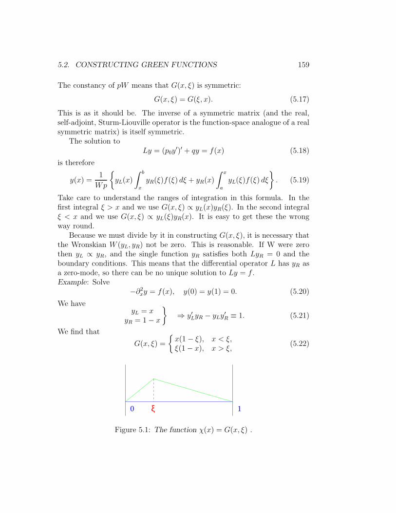
5.2. CONSTRUCTING GREEN FUNCTIONS 159
The constancy of pW means that G(x, ξ) is symmetric:
G(x, ξ) = G(ξ, x). (5.17)
This is as it should be. The inverse of a symmetric matrix (and the real,self-adjoint, Sturm-Liouville operator is the function-space analogue of a realsymmetric matrix) is itself symmetric.
The solution toLy = (p0y
′)′ + qy = f(x) (5.18)
is therefore
y(x) =1
Wp
yL(x)
∫ b
x
yR(ξ)f(ξ) dξ + yR(x)
∫ x
a
yL(ξ)f(ξ) dξ
. (5.19)
Take care to understand the ranges of integration in this formula. In thefirst integral ξ > x and we use G(x, ξ) ∝ yL(x)yR(ξ). In the second integralξ < x and we use G(x, ξ) ∝ yL(ξ)yR(x). It is easy to get these the wrongway round.
Because we must divide by it in constructing G(x, ξ), it is necessary thatthe Wronskian W (yL, yR) not be zero. This is reasonable. If W were zerothen yL ∝ yR, and the single function yR satisfies both LyR = 0 and theboundary conditions. This means that the differential operator L has yR asa zero-mode, so there can be no unique solution to Ly = f .Example: Solve
−∂2xy = f(x), y(0) = y(1) = 0. (5.20)
We haveyL = x
yR = 1− x
⇒ y′LyR − yLy′R ≡ 1. (5.21)
We find that
G(x, ξ) =
x(1− ξ), x < ξ,ξ(1− x), x > ξ,
(5.22)
0 1ξ
Figure 5.1: The function χ(x) = G(x, ξ) .

160 CHAPTER 5. GREEN FUNCTIONS
and
y(x) = (1− x)∫ x
0
ξf(ξ) dξ + x
∫ 1
x
(1− ξ)f(ξ) dξ. (5.23)
5.2.2 Initial-value problems
Initial value problems are those boundary-value problems where all boundaryconditions are imposed at one end of the interval, instead of some conditionsat one end and some at the other. The same ingredients go into to construct-ing the Green function, though.
Consider the problem
dy
dt−Q(t)y = F (t), y(0) = 0. (5.24)
We seek a Green function such that
LtG(t, t′) ≡
(d
dt−Q(t)
)G(t, t′) = δ(t− t′) (5.25)
and G(0, t′) = 0.
We need χ(t) = G(t, t′) to satisfy Ltχ = 0, except at t = t′, and needχ(0) = 0. The unique solution of Ltχ = 0 with χ(0) = 0 is χ(t) ≡ 0. Thismeans that G(t, 0) = 0 for all t < t′. Near t = t′ we have the jump condition
G(t′ + ε, t′)−G(t′ − ε, t′) = 1. (5.26)
The unique solution is
G(t, t′) = θ(t− t′) exp∫ t
t′Q(s)ds
, (5.27)
where θ(t− t′) is the Heaviside step distribution
θ(t) =
0, t < 0,1, t > 0.
(5.28)

5.2. CONSTRUCTING GREEN FUNCTIONS 161
1
t
t’
G(t,t’)
Figure 5.2: The Green functionG(t, t′) for the first-order initial value problem.
Therefore
y(t) =
∫ ∞
0
G(t, t′)F (t′)dt′,
=
∫ t
0
exp
∫ t
t′Q(s) ds
F (t′) dt′
= exp
∫ t
0
Q(s) ds
∫ t
0
exp
−∫ t′
0
Q(s) ds
F (t′) dt′. (5.29)
We earlier obtained this solution via variation of parameters.Example: Forced, Damped, Harmonic Oscillator. An oscillator obeys theequation
x+ 2γx+ (Ω2 + γ2)x = F (t). (5.30)
Here γ > 0 is the friction coeffecient. Assuming that the oscillator is at restat the origin at t = 0, we will show that
x(t) =
(1
Ω
)∫ t
0
e−γ(t−τ) sinΩ(t− τ)F (τ)dτ. (5.31)
We seek a Green function G(t, τ) such that χ(t) = G(t, τ) obeys χ(0) =χ′(0) = 0. Again, the unique solution of the differential equation with thisinitial data is χ(t) ≡ 0. The Green function must be continuous at t = τ ,but its derivative must be discontinuous there, jumping from zero to unityto provide the delta function. Thereafter, it must satisfy the homogeneousequation. The unique function satisfying all these requirements is
G(t, τ) = θ(t− τ) 1Ωe−γ(t−τ) sin Ω(t− τ). (5.32)

162 CHAPTER 5. GREEN FUNCTIONS
τt
G(t, τ )
Figure 5.3: The Green function G(t, τ) for the damped oscillator problem .
Both these initial-value Green functions G(t, t′) are identically zero whent < t′. This is because the Green function is the response of the system to akick at time t = t′, and in physical problems no effect comes before its cause.Such Green functions are said to be causal .
Physics application: friction without friction—the Caldeira-Leggettmodel in real time.
We now describe an application of the initial-value problem Green functionwe found in the preceding example.
When studying the quantum mechanics of systems with friction, such asthe viscously damped oscillator, we need a tractable model of the dissipativeprocess. Such a model was introduced by Caldeira and Leggett.1 Theyconsider the Lagrangian
L =1
2
(Q2 − (Ω2 −∆Ω2)Q2
)−Q
∑
i
fiqi +∑
i
1
2
(q2i − ω2
i q2i
), (5.33)
which describes a macroscopic variable Q(t), linearly coupled to an oscillatorbath of very many simple systems qi representing the environment. Thequantity
∆Ω2 def= −
∑
i
(f 2i
ω2i
), (5.34)
1A. Caldiera, A. J. Leggett, Phys. Rev. Lett. 46 (1981) 211.

5.2. CONSTRUCTING GREEN FUNCTIONS 163
is a counter-term that is inserted to cancel the frequency shift
Ω2 → Ω2 −∑
i
(f 2i
ω2i
), (5.35)
caused by the coupling to the bath.2
The equations of motion are
Q+ (Ω2 −∆Ω2)Q +∑
i
fiqi = 0,
qi + ω2i qi + fiQ = 0. (5.36)
Using our initial-value Green function, we solve for the qi in terms of Q(t):
fiqi = −∫ t
−∞
(f 2i
ωi
)sinωi(t− τ)Q(τ)dτ. (5.37)
The resulting motion of the qi feeds back into the equation for Q to give
Q+ (Ω2 −∆Ω2)Q+
∫ t
−∞F (t− τ)Q(τ) dτ = 0, (5.38)
where
F (t)def= −
∑
i
(f 2i
ωi
)sin(ωit) (5.39)
is a memory function.It is now convenient to introduce a spectral function
J(ω)def=π
2
∑
i
(f 2i
ωi
)δ(ω − ωi), (5.40)
which characterizes the spectrum of couplings and frequencies associatedwith the oscillator bath. In terms of J(ω) we can write
F (t) = −2
π
∫ ∞
0
J(ω) sin(ωt) dω. (5.41)
2The shift arises because a static Q displaces the bath oscillators so that fiqi =−(f2
i /ω2i )Q. Substituting these values for the fiqi into the potential terms shows that, in
the absence of ∆Ω2Q2, the effective potential seen by Q would be
1
2Ω2Q2 +Q
∑
i
fiqi +∑
i
1
2ω2i q
2i =
1
2
(Ω2 −
∑
i
(f2i
ω2i
))Q2.

164 CHAPTER 5. GREEN FUNCTIONS
Although J(ω) is defined as a sum of delta function “spikes,” the oscillatorbath contains a very large number of systems and this makes J(ω) effectivelya smooth function. This is just as the density of a gas (a sum of deltafunctions at the location of the atoms) is macroscopically smooth. By takingdifferent forms for J(ω) we can represent a wide range of environments.Caldeira and Leggett show that to obtain a friction force proportional toQ we should make J(ω) proportional to the frequency ω. To see how thisworks, consider the choice
J(ω) = ηω
[Λ2
Λ2 + ω2
], (5.42)
which is equal to ηω for small ω, but tends to zero when ω >> Λ. Thehigh-frequency cutoff Λ is introduced to make the integrals over ω converge.With this cutoff
2
π
∫ ∞
0
J(ω) sin(ωt) dω =2
2πi
∫ ∞
−∞
η ωΛ2eiωt
Λ2 + ω2dω = sgn (t)ηΛ2e−Λ|t|. (5.43)
Therefore,∫ t
−∞F (t− τ)Q(τ) dτ = −
∫ t
−∞ηΛ2e−Λ|t−τ |Q(τ) dτ
= −ηΛQ(t) + ηQ(t)− η
2ΛQ(t) + · · · , (5.44)
where the second line results from expanding Q(τ) as a Taylor series
Q(τ) = Q(t) + (τ − t)Q(t) + · · · , (5.45)
and integrating term-by-term. Now,
−∆Ω2 ≡∑
i
(f 2i
ω2i
)=
2
π
∫ ∞
0
J(ω)
ωdω =
2
π
∫ ∞
0
ηΛ2
Λ2 + ω2dω = ηΛ. (5.46)
The −∆Ω2Q counter-term thus cancels the leading term −ηΛQ(t) in (5.44),which would otherwise represent a Λ-dependent frequency shift. After thiscancellation we can safely let Λ → ∞, and so ignore terms with negativepowers of the cutoff. The only surviving term in (5.44) is then ηQ. Thiswe substitute into (5.38), which becomes the equation for viscously dampedmotion:
Q + ηQ+ Ω2Q = 0. (5.47)

5.2. CONSTRUCTING GREEN FUNCTIONS 165
The oscillators in the bath absorb energy but, unlike a pair of coupled oscil-lators which trade energy rhythmically back-and-forth, the incommensuratemotion of the many qi prevents them from cooperating for long enough toreturn any energy to Q(t).
5.2.3 Modified Green function
When the equation Ly = 0 has a non trivial-solution, there can be no uniquesolution to Ly = f , but there still will be solutions provided f is orthogonalto all solutions of L†y = 0.Example: Consider
Ly ≡ −∂2xy = f(x), y′(0) = y′(1) = 0. (5.48)
The equation Ly = 0 has one non-trivial solution, y(x) = 1. The operatorL is self-adjoint, L† = L, and so there will be solutions to Ly = f provided〈1, f〉 =
∫ 1
0f dx = 0.
We cannot define the the green function as a solution to
−∂2xG(x, ξ) = δ(x− ξ), (5.49)
because∫ 1
0δ(x− ξ) dx = 1 6= 0, but we can seek a solution to
−∂2xG(x, ξ) = δ(x− ξ)− 1 (5.50)
as the right-hand integrates to zero.A general solution to −∂2xy = −1 is
y = A+Bx+1
2x2, (5.51)
and the functions
yL = A+1
2x2,
yR = C − x+ 1
2x2, (5.52)
obey the boundary conditions at the left and right ends of the interval, re-spectively. Continuity at x = ξ demands that A = C − ξ, and we are leftwith
G(x, ξ) =
C − ξ + 1
2x2, 0 < x < ξ
C − x+ 12x2, ξ < x < 1,
(5.53)

166 CHAPTER 5. GREEN FUNCTIONS
There is no freedom left to impose the condition
G′(ξ − ε, ξ)−G′(ξ + ε, ξ) = 1, (5.54)
but it is automatically satisfied ! Indeed,
G′(ξ − ε, ξ) = ξ
G′(ξ + ε, ξ) = −1 + ξ. (5.55)
We may select a different value of C for each ξ, and a convenient choiceis
C =1
2ξ2 +
1
3(5.56)
which makes G symmetric:
G(x, ξ) =
13− ξ + x2+ξ2
2, 0 < x < ξ
13− x+ x2+ξ2
2, ξ < x < 1,
. (5.57)
It also makes∫ 1
0G(x, ξ) dx = 0.
ξ
Figure 5.4: The modified Green function.
The solution to Ly = f is
y(x) =
∫ 1
0
G(x, ξ)f(ξ) dξ + A, (5.58)
where A is arbitrary.

5.3. APPLICATIONS OF LAGRANGE’S IDENTITY 167
5.3 Applications of Lagrange’s Identity
5.3.1 Hermiticity of Green function
Earlier we noted the symmetry of the Green function for the Sturm-Liouvilleequation. We will now establish the corresponding result for general differ-ential operators.
Let G(x, ξ) obey LxG(x, ξ) = δ(x− ξ) with homogeneous boundary con-ditions B, and let G†(x, ξ) obey L†
xG†(x, ξ) = δ(x−ξ) with adjoint boundary
conditions B†. Then, from Lagrange’s identity, we have
[Q(G,G†)]ba =
∫ b
a
dx(L†xG
†(x, ξ))∗G(x, ξ′)− (G†(x, ξ))∗LG(x, ξ′)
=
∫ b
a
dxδ(x− ξ)G(x, ξ′)−
(G†(x, ξ)
)∗δ(x− ξ′)
= G(ξ, ξ′)−(G†(ξ′, ξ)
)∗. (5.59)
Thus, provided [Q(G,G†)]ba = 0, which is indeed the case because the bound-ary conditions for L, L† are mutually adjoint, we have
G†(ξ, x) =(G(x, ξ)
)∗, (5.60)
and the Green functions, regarded as matrices with continuous rows andcolumns, are Hermitian conjugates of one another.
Example: Let
L =d
dx, D(L) = y, Ly ∈ L2[0, 1] : y(0) = 0. (5.61)
In this case G(x, ξ) = θ(x− ξ).Now, we have
L† = − d
dx, D(L) = y, Ly ∈ L2[0, 1] : y(1) = 0 (5.62)
and G†(x, ξ) = θ(ξ − x).

168 CHAPTER 5. GREEN FUNCTIONS
0 1 0 1
1 1
ξ ξ
Figure 5.5: G(x, ξ) = θ(x− ξ), and G†(x, ξ) = θ(ξ − x).
5.3.2 Inhomogeneous boundary conditions
Our differential operators have been defined with linear homogeneous bound-ary conditions. We can, however, use them, and their Green-function in-verses, to solve differential equations with inhomogeneous boundary condi-tions.
Suppose, for example, we wish to solve
−∂2xy = f(x), y(0) = a, y(1) = b. (5.63)
We already know the Green function for the homogeneous boundary-conditionproblem with operator
L = −∂2x, D(L) = y, Ly ∈ L2[0, 1] : y(0) = 0, y(1) = 0. (5.64)
It is
G(x, ξ) =
x(1− ξ), x < ξ,ξ(1− x), x > ξ.
(5.65)
Now we apply Lagrange’s identity to χ(x) = G(x, ξ) and y(x) to get
∫ 1
0
dxG(x, ξ)
(−∂2xy(x)
)− y(x)
(−∂2xG(x, ξ)
)= [G′(x, ξ)y(x)−G(x, ξ)y′(x)]10.
(5.66)Here, as usual, G′(x, ξ) = ∂xG(x, ξ). The integral is equal to
∫dx G(x, ξ)f(x)− y(x)δ(x− ξ) =
∫G(x, ξ)f(x) dx− y(ξ), (5.67)
whilst the integrated-out bit is
−(1− ξ)y(0)− 0 y′(0)− ξy(1) + 0 y′(1). (5.68)

5.3. APPLICATIONS OF LAGRANGE’S IDENTITY 169
Therefore, we have
y(ξ) =
∫G(x, ξ)f(x) dx+ (1− ξ)y(0) + ξy(1). (5.69)
Here the term with f(x) is the particular integral, whilst the remaining termsconstitute the complementary function (obeying the differential equationwithout the source term) which serves to satisfy the boundary conditions.Observe that the arguments in G(x, ξ) are not in the usual order, but, in thepresent example, this does not matter because G is symmetric.
When the operator L is not self-adjoint, we need to distinguish betweenL and L†, and G and G†. We then apply Lagrange’s identity to the unknownfunction u(x) and χ(x) = G†(x, ξ).Example: We will use the Green-function method to solve the differentialequation
du
dx= f(x), x ∈ [0, 1], u(0) = a. (5.70)
We can, of course, write down the answer to this problem directly, but itis interesting to see how the general strategy produces the solution. Wefirst find the Green function G(x, ξ) for the operator with the correspondinghomogeneous boundary conditions. In the present case, this operator is
L = ∂x, D(L) = u, Lu ∈ L2[0, 1] : u(0) = 0, (5.71)
and the appropriate Green function is G(x, ξ) = θ(x − ξ). From G we then
read off the adjoint Green function as G†(x, ξ) =(G(ξ, x)
)∗. In the present
example, we have G†(x,′ x) = θ(ξ − x). We now use Lagrange’s identity inthe form∫ 1
0
dx(L†xG
†(x, ξ))∗u(x)−
(G†(x, ξ)
)∗Lxu(x)
=[Q(G†, u
)]10. (5.72)
In all cases, the left hand side is equal to∫ 1
0
dxδ(x− ξ)u(x)−GT (x, ξ)f(x)
, (5.73)
where T denotes transpose, GT (x, ξ) = G(ξ, x). The left hand side is there-fore equal to
u(ξ)−∫ 1
0
dxG(ξ, x)f(x). (5.74)

170 CHAPTER 5. GREEN FUNCTIONS
The right hand side depends on the details of the problem. In the presentcase, the integrated out part is
[Q(G†, u)
]10= −
[GT (x, ξ)u(x)
]10= u(0). (5.75)
At the last step we have used the specific form GT (x, ξ) = θ(ξ − x) to findthat only the lower limit contributes. The end result is therefore the expectedone:
u(y) = u(0) +
∫ y
0
f(x) dx. (5.76)
Variations of this strategy enable us to solve any inhomogeneous boundary-value problem in terms of the Green function for the corresponding homoge-neous boundary-value problem.
5.4 Eigenfunction Expansions
Self-adjoint operators possess a complete set of eigenfunctions, and we canexpand the Green function in terms of these. Let
Lϕn = λnϕn. (5.77)
Let us further suppose that none of the λn are zero. Then the Green functionhas the eigenfunction expansion
G(x, ξ) =∑
n
ϕn(x)ϕ∗n(ξ)
λn. (5.78)
That this is so follows from
Lx
(∑
n
ϕn(x)ϕ∗n(ξ)
λn
)=
∑
n
(Lxϕn(x)
)ϕ∗n(ξ)
λn
=∑
n
λnϕn(x)ϕ∗n(ξ)
λn
=∑
n
ϕn(x)ϕ∗n(ξ)
= δ(x− ξ). (5.79)

5.5. ANALYTIC PROPERTIES OF GREEN FUNCTIONS 171
Example: : Consider our familiar exemplar
L = −∂2x, D(L) = y, Ly ∈ L2[0, 1] : y(0) = y(1) = 0, (5.80)
for which
G(x, ξ) =
x(1− ξ), x < ξ,ξ(1− x), x > ξ.
(5.81)
Computing the Fourier series shows that
G(x, ξ) =
∞∑
n=1
(2
n2π2
)sin(nπx) sin(nπξ). (5.82)
Modified Green function
When one or more of the eigenvalues is zero, a modified Green function isobtained by simply omitting the corresponding terms from the series.
Gmod(x, ξ) =∑
λn 6=0
ϕn(x)ϕ∗n(ξ)
λn. (5.83)
Then
LxGmod(x, ξ) = δ(x− ξ)−∑
λn=0
ϕn(x)ϕ∗n(ξ). (5.84)
We see that this Gmod is still hermitian, and, as a function of x, is orthogonalto the zero modes. These are the properties we elected when constructingthe modified Green function in equation (5.57).
5.5 Analytic Properties of Green Functions
In this section we study the properties of Green functions considered asfunctions of a complex variable. Some of the formulæ are slightly easier toderive using contour integral methods, but these are not necessary and we willnot use them here. The only complex-variable prerequisite is a familiaritywith complex arithmetic and, in particular, knowledge of how to take thelogarithm and the square root of a complex number.
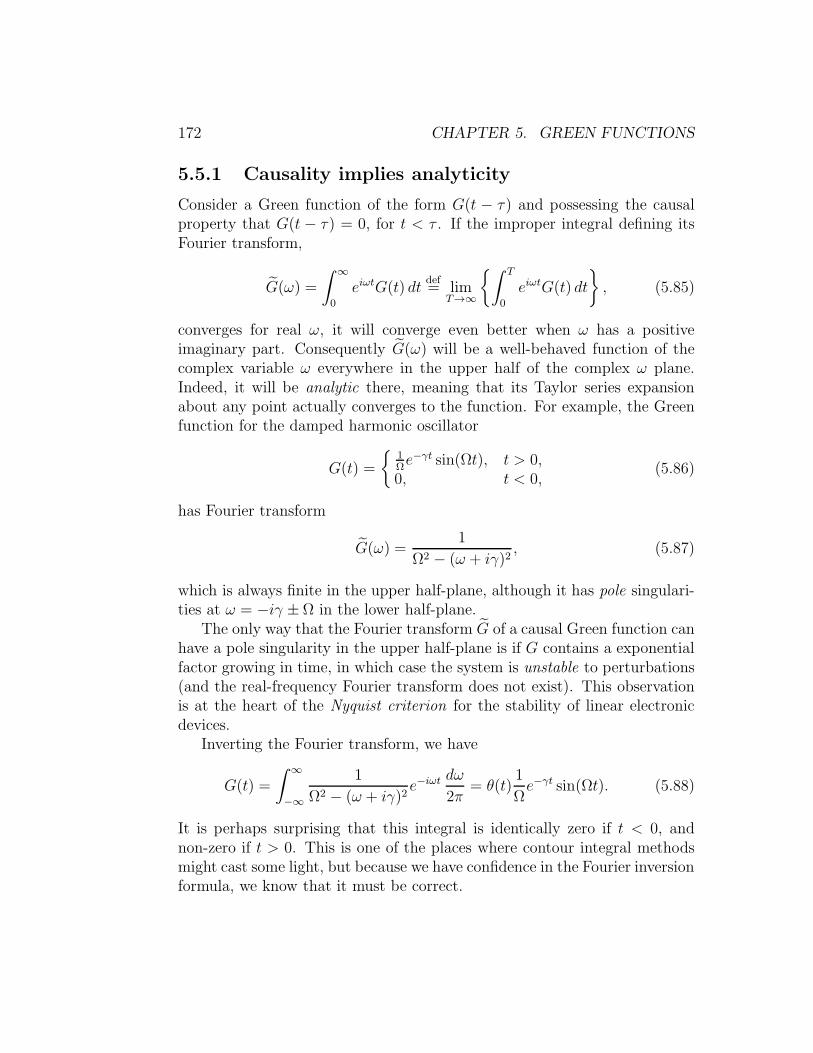
172 CHAPTER 5. GREEN FUNCTIONS
5.5.1 Causality implies analyticity
Consider a Green function of the form G(t − τ) and possessing the causalproperty that G(t − τ) = 0, for t < τ . If the improper integral defining itsFourier transform,
G(ω) =
∫ ∞
0
eiωtG(t) dtdef= lim
T→∞
∫ T
0
eiωtG(t) dt
, (5.85)
converges for real ω, it will converge even better when ω has a positiveimaginary part. Consequently G(ω) will be a well-behaved function of thecomplex variable ω everywhere in the upper half of the complex ω plane.Indeed, it will be analytic there, meaning that its Taylor series expansionabout any point actually converges to the function. For example, the Greenfunction for the damped harmonic oscillator
G(t) =
1Ωe−γt sin(Ωt), t > 0,
0, t < 0,(5.86)
has Fourier transform
G(ω) =1
Ω2 − (ω + iγ)2, (5.87)
which is always finite in the upper half-plane, although it has pole singulari-ties at ω = −iγ ± Ω in the lower half-plane.
The only way that the Fourier transform G of a causal Green function canhave a pole singularity in the upper half-plane is if G contains a exponentialfactor growing in time, in which case the system is unstable to perturbations(and the real-frequency Fourier transform does not exist). This observationis at the heart of the Nyquist criterion for the stability of linear electronicdevices.
Inverting the Fourier transform, we have
G(t) =
∫ ∞
−∞
1
Ω2 − (ω + iγ)2e−iωt
dω
2π= θ(t)
1
Ωe−γt sin(Ωt). (5.88)
It is perhaps surprising that this integral is identically zero if t < 0, andnon-zero if t > 0. This is one of the places where contour integral methodsmight cast some light, but because we have confidence in the Fourier inversionformula, we know that it must be correct.

5.5. ANALYTIC PROPERTIES OF GREEN FUNCTIONS 173
Remember that in deriving (5.88) we have explicitly assumed that thedamping coefficient γ is positive. It is important to realize that reversing thesign of γ on the left-hand side of (5.88) does more than just change e−γt → eγt
on the right-hand side. Naıvely setting γ → −γ on both sides of (5.88) givesan equation that cannot possibly be true. The left-hand side would be theFourier transform of a smooth function, and the Riemann-Lebesgue lemmatells us that such a Fourier transform must become zero when |t| → ∞. Theright-hand side, to the contrary, would be a function whose oscillations growwithout bound as t becomes large and positive.
To find the correct equation, observe that we can legitimately effect thesign-change γ → −γ by first complex-conjugating the integral and thenchanging t to −t. Performing these two operations on both sides of (5.88)leads to ∫ ∞
−∞
1
Ω2 − (ω − iγ)2 e−iωt dω
2π= −θ(−t) 1
Ωeγt sin(Ωt) (5.89)
The new right-hand side represents an exponentially growing oscillation thatis suddenly silenced by the kick at t = 0.
ιγ= +ιε ιγ=−ιε
t tt=0 t=0
Figure 5.6: The effect on G(t), the Green function of an undamped oscillator,of changing iγ from +iε to −iε.
The effect of taking the damping parameter γ from an infitesimally smallpostive value ε to an infinitesimally small negative value −ε is therefore toturn the causal Green function (no motion before it is started by the delta-function kick) of the undamped oscillator into an anti-causal Green function(no motion after it is stopped by the kick). Ultimately, this is because the thedifferential operator corresponding to a harmonic oscillator with initial -valuedata is not self-adjoint, and its adjoint operator corresponds to a harmonicoscillator with final -value data.

174 CHAPTER 5. GREEN FUNCTIONS
This discontinuous dependence on an infinitesimal damping parameter isthe subject of the next few sections.
Physics application: Caldeira-Leggett in frequency space
If we write the Caldeira-Leggett equations of motion (5.36) in Fourier fre-quency space by setting
Q(t) =
∫ ∞
−∞
dω
2πQ(ω)e−iωt, (5.90)
and
qi(t) =
∫ ∞
−∞
dω
2πqi(ω)e
−iωt, (5.91)
we have (after including an external force Fext to drive the system)(−ω2 + (Ω2 −∆Ω2)
)Q(ω)−
∑
i
fiqi(ω) = Fext(ω),
(−ω2 + ω2i )qi(ω) + fiQ(ω) = 0. (5.92)
Eliminating the qi, we obtain
(−ω2 + (Ω2 −∆Ω2)
)Q(ω)−
∑
i
f 2i
ω2i − ω2
Q(ω) = Fext(ω). (5.93)
As before, sums over the index i are replaced by integrals over the spectralfunction ∑
i
f 2i
ω2i − ω2
→ 2
π
∫ ∞
0
ω′J(ω′)
ω′2 − ω2dω′, (5.94)
and
−∆Ω2 ≡∑
i
(f 2i
ω2i
)→ 2
π
∫ ∞
0
J(ω′)
ω′ dω′. (5.95)
Then
Q(ω) =
(1
Ω2 − ω2 +Π(ω)
)Fext(ω), (5.96)
where the self-energy Π(ω) is given by
Π(ω) =2
π
∫ ∞
0
J(ω′)
ω′ −ω′J(ω′)
ω′2 − ω2
dω′ = −ω2 2
π
∫ ∞
0
J(ω′)
ω′(ω′2 − ω2)dω′.
(5.97)

5.5. ANALYTIC PROPERTIES OF GREEN FUNCTIONS 175
The expression
G(ω) ≡ 1
Ω2 − ω2 +Π(ω)(5.98)
a typical response function. Analogous objects occur in all branches ofphysics.
For viscous damping we know that J(ω) = ηω. Let us evaluate theintegral occuring in Π(ω) for this case:
I(ω) =
∫ ∞
0
dω′
ω′2 − ω2. (5.99)
We will initially assume that ω is positive. Now,
1
ω′2 − ω2=
1
2ω
(1
ω′ − ω −1
ω′ + ω
), (5.100)
so
I(ω) =
[1
2ω
(ln(ω′ − ω)− ln(ω′ + ω)
)]∞
ω′=0
. (5.101)
At the upper limit we have ln((∞− ω)/(∞ + ω)
)= ln 1 = 0. The lower
limit contributes
− 1
2ω
(ln(−ω)− ln(ω)
). (5.102)
To evaluate the logarithm of a negative quantity we must use
lnω = ln |ω|+ i arg ω, (5.103)
where we will take arg ω to lie in the range −π < argω < π.
Im
Re
arg
ω
(−ω)
ω−ω
ω
Figure 5.7: When ω has a small positive imaginary part, arg (−ω) ≈ −π.

176 CHAPTER 5. GREEN FUNCTIONS
To get an unambiguous answer, we need to give ω an infinitesimal imaginarypart ±iε. Depending on the sign of this imaginary part, we find that
I(ω ± iε) = ± iπ2ω. (5.104)
This formula remains true when the real part of ω is negative, and so
Π(ω ± iε) = ∓iηω. (5.105)
Now the frequency-space version of
Q(t) + ηQ+ Ω2Q = Fext(t) (5.106)
is(−ω2 − iηω + Ω2)Q(ω) = Fext(ω), (5.107)
so we must opt for the small shift in ω that leads to Π(ω) = −iηω. Thismeans that we must regard ω as having a positive infinitesimal imaginarypart, ω → ω+ iε. This imaginary part is a good and needful thing: it effectsthe replacement of the ill-defined singular integrals
G(t)?=
∫ ∞
0
1
ω2i − ω2
e−iωt dω, (5.108)
which arise as we transform back to real time, with the unambiguous expres-sions
Gε(t) =
∫ ∞
0
1
ω2i − (ω + iε)2
e−iωt dω. (5.109)
The latter, we know, give rise to properly causal real-time Green functions.
5.5.2 Plemelj formulæ
The functions we are meeting can all be cast in the form
f(ω) =1
π
∫ b
a
ρ(ω′)
ω′ − ω dω′. (5.110)
If ω lies in the integration range [a, b], then we divide by zero as we integrateover ω′ = ω. We ought to avoid doing this, but this interval is often exactlywhere we desire to evaluate f . As before, we evade the division by zero by
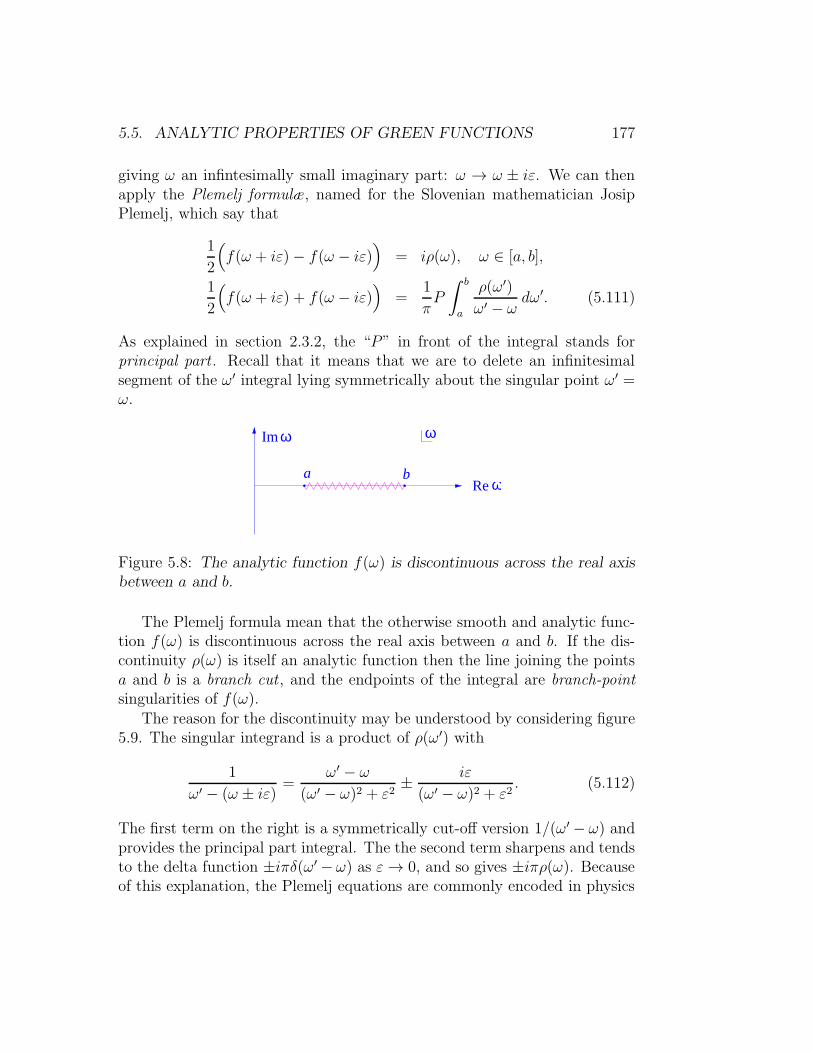
5.5. ANALYTIC PROPERTIES OF GREEN FUNCTIONS 177
giving ω an infintesimally small imaginary part: ω → ω ± iε. We can thenapply the Plemelj formulæ, named for the Slovenian mathematician JosipPlemelj, which say that
1
2
(f(ω + iε)− f(ω − iε)
)= iρ(ω), ω ∈ [a, b],
1
2
(f(ω + iε) + f(ω − iε)
)=
1
πP
∫ b
a
ρ(ω′)
ω′ − ω dω′. (5.111)
As explained in section 2.3.2, the “P” in front of the integral stands forprincipal part . Recall that it means that we are to delete an infinitesimalsegment of the ω′ integral lying symmetrically about the singular point ω′ =ω.
a bω
ω ωIm
Re
Figure 5.8: The analytic function f(ω) is discontinuous across the real axisbetween a and b.
The Plemelj formula mean that the otherwise smooth and analytic func-tion f(ω) is discontinuous across the real axis between a and b. If the dis-continuity ρ(ω) is itself an analytic function then the line joining the pointsa and b is a branch cut , and the endpoints of the integral are branch-pointsingularities of f(ω).
The reason for the discontinuity may be understood by considering figure5.9. The singular integrand is a product of ρ(ω′) with
1
ω′ − (ω ± iε) =ω′ − ω
(ω′ − ω)2 + ε2± iε
(ω′ − ω)2 + ε2. (5.112)
The first term on the right is a symmetrically cut-off version 1/(ω′− ω) andprovides the principal part integral. The the second term sharpens and tendsto the delta function ±iπδ(ω′− ω) as ε→ 0, and so gives ±iπρ(ω). Becauseof this explanation, the Plemelj equations are commonly encoded in physics

178 CHAPTER 5. GREEN FUNCTIONS
papers via the “iε” cabbala
1
ω′ − (ω ± iε) = P
(1
ω′ − ω
)± iπδ(ω′ − ω). (5.113)
.
ωω
Im gRe g
ω ω
Figure 5.9: Sketch of the real and imaginary parts of g(ω′) = 1/(ω′−(ω+iε)).
If ρ is real, as it often is, then f(ω+iη) =(f(ω−iη)
)∗. The discontinuity
across the real axis is then purely imaginary, and
1
2
(f(ω + iε) + f(ω − iε)
)(5.114)
is the real part of f . In this case we can write (5.110) as
Re f(ω) =1
πP
∫ b
a
Im f(ω′)
ω′ − ω dω′. (5.115)
This formula is typical of the relations linking the real and imaginary partsof causal response functions.
A practical example of such a relation is provided by the complex, frequency-dependent, refractive index , n(ω), of a medium. This is defined so that atravelling electromagnetic wave takes the form
E(x, t) = E0 ein(ω)kx−iωt. (5.116)
Here, k = ω/c is the in vacuuo wavenumber. We can decompose n into itsreal and imaginary parts:
n(ω) = nR + inI
= nR(ω) +i
2|k|γ(ω), (5.117)
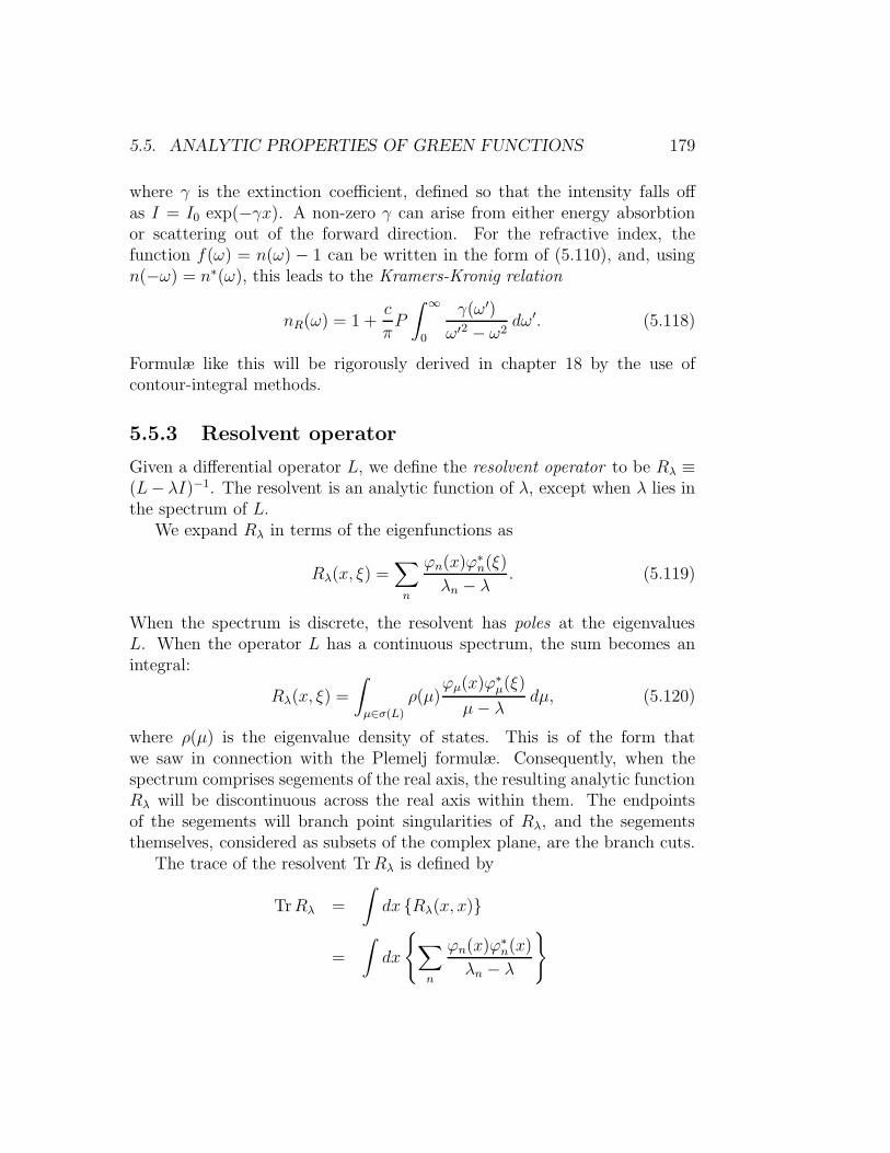
5.5. ANALYTIC PROPERTIES OF GREEN FUNCTIONS 179
where γ is the extinction coefficient, defined so that the intensity falls offas I = I0 exp(−γx). A non-zero γ can arise from either energy absorbtionor scattering out of the forward direction. For the refractive index, thefunction f(ω) = n(ω) − 1 can be written in the form of (5.110), and, usingn(−ω) = n∗(ω), this leads to the Kramers-Kronig relation
nR(ω) = 1 +c
πP
∫ ∞
0
γ(ω′)
ω′2 − ω2dω′. (5.118)
Formulæ like this will be rigorously derived in chapter 18 by the use ofcontour-integral methods.
5.5.3 Resolvent operator
Given a differential operator L, we define the resolvent operator to be Rλ ≡(L− λI)−1. The resolvent is an analytic function of λ, except when λ lies inthe spectrum of L.
We expand Rλ in terms of the eigenfunctions as
Rλ(x, ξ) =∑
n
ϕn(x)ϕ∗n(ξ)
λn − λ. (5.119)
When the spectrum is discrete, the resolvent has poles at the eigenvaluesL. When the operator L has a continuous spectrum, the sum becomes anintegral:
Rλ(x, ξ) =
∫
µ∈σ(L)ρ(µ)
ϕµ(x)ϕ∗µ(ξ)
µ− λ dµ, (5.120)
where ρ(µ) is the eigenvalue density of states. This is of the form thatwe saw in connection with the Plemelj formulæ. Consequently, when thespectrum comprises segements of the real axis, the resulting analytic functionRλ will be discontinuous across the real axis within them. The endpointsof the segements will branch point singularities of Rλ, and the segementsthemselves, considered as subsets of the complex plane, are the branch cuts.
The trace of the resolvent TrRλ is defined by
TrRλ =
∫dx Rλ(x, x)
=
∫dx
∑
n
ϕn(x)ϕ∗n(x)
λn − λ

180 CHAPTER 5. GREEN FUNCTIONS
=∑
n
1
λn − λ
→∫
ρ(µ)
µ− λ dµ. (5.121)
Applying Plemelj to Rλ, we have
Im[limε→0
TrRλ+iε
]= πρ(λ). (5.122)
Here, we have used that fact that ρ is real, so
TrRλ−iε =(TrRλ+iε
)∗. (5.123)
The non-zero imaginary part therefore shows that Rλ is discontinuous acrossthe real axis at points lying in the continuous spectrum.Example: Consider
L = −∂2x +m2, D(L) = y, Ly ∈ L2[−∞,∞]. (5.124)
As we know, this operator has a continuous spectrum, with eigenfunctions
ϕk =1√Leikx. (5.125)
Here, L is the (very large) length of the interval. The eigenvalues are E =k2 + m2, so the spectrum is all positive numbers greater than m2. Themomentum density of states is
ρ(k) =L
2π. (5.126)
The completeness relation is∫ ∞
−∞
dk
2πeik(x−ξ) = δ(x− ξ), (5.127)
which is just the Fourier integral formula for the delta function.The Green function for L is
G(x− y) =∫ ∞
−∞dk
(dn
dk
)ϕk(x)ϕ
∗k(y)
k2 +m2=
∫ ∞
−∞
dk
2π
eik(x−y)
k2 +m2=
1
2me−m|x−y|.
(5.128)

5.5. ANALYTIC PROPERTIES OF GREEN FUNCTIONS 181
−λ
Im
Re
λ
λarg(−λ)/2
λ
−λ
Figure 5.10: If Imλ > 0, and with the branch cut for√z in its usual place
along the negative real axis, then√−λ has negative imaginary part and
positive real part.
We can use the same calculation to look at the resolvent Rλ = (−∂2x − λ)−1.Replacing m2 by −λ, we have
Rλ(x, y) =1
2√−λ
e−√−λ|x−y|. (5.129)
To appreciate this expression, we need to know how to evaluate√z where
z is complex. We write z = |z|eiφ where we require −π < φ < π. We nowdefine √
z =√|z|eiφ/2. (5.130)
When we evaluate√z for z just below the negative real axis then this defini-
tion gives −i√|z|, and just above the axis we find +i
√|z|. The discontinuity
means that the negative real axis is a branch cut for the the square-root func-tion. The
√−λ’s appearing in Rλ therefore mean that the positive real axis
will be a branch cut for Rλ. This branch cut therefore coincides with thespectrum of L, as promised earlier.If λ is positive and we shift λ→ λ+ iε then
1
2√−λ
e−√−λ|x−y| → i
2√λe+i
√λ|x−y|−ε|x−y|/2
√λ. (5.131)
Notice that this decays away as |x − y| → ∞. The square root retains apositive real part when λ is shifted to λ− iε, and so the decay is still present:
1
2√−λe
−√−λ|x−y| → − i
2√λe−i
√λ|x−y|−ε|x−y|/2
√λ. (5.132)

182 CHAPTER 5. GREEN FUNCTIONS
In each case, with λ either immediately above or immediately below thecut, the small imaginary part tempers the oscillatory behaviour of the Greenfunction so that χ(x) = G(x, y) is square integrable and remains an elementof L2[R].
We now take the trace of R by setting x = y and integrating:
TrRλ+iε = iπL
2π√|λ|. (5.133)
Thus,
ρ(λ) = θ(λ)L
2π√|λ|, (5.134)
which coincides with our direct calculation.
Example: Let
L = −i∂x, D(L) = y, Ly ∈ L2[R]. (5.135)
This has eigenfunctions eikx with eigenvalues k. The spectrum is thereforethe entire real line. The local eigenvalue density of states is 1/2π. Theresolvent is therefore
(−i∂x − λ)−1x,ξ =
1
2π
∫ ∞
−∞eik(x−ξ)
1
k − λdk. (5.136)
To evaluate this, first consider the Fourier transforms of
F1(x) = θ(x)e−κx,
F2(x) = −θ(−x)eκx, (5.137)
where κ is a positive real number.
xx
1
−1
Figure 5.11: The functions F1(x) = θ(x)e−κx and F2(x) = −θ(−x)eκx .

5.5. ANALYTIC PROPERTIES OF GREEN FUNCTIONS 183
We have ∫ ∞
−∞
θ(x)e−κx
e−ikx dx =
1
i
1
k − iκ , (5.138)
∫ ∞
−∞
−θ(−x)eκx
e−ikx dx =
1
i
1
k + iκ. (5.139)
Inverting the transforms gives
θ(x)e−κx =1
2πi
∫ ∞
−∞
1
k − iκeikx dk,
−θ(−x)eκx =1
2πi
∫ ∞
−∞
1
k + iκeikx dk. (5.140)
These are important formulæ in their own right, and you should take careto understand them. Now we apply them to evaluating the integral definingRλ.
If we write λ = µ+ iν, we find
1
2π
∫ ∞
−∞eik(x−ξ)
1
k − λ dk =
iθ(x− ξ)eiµ(x−ξ)e−ν(x−ξ), ν > 0,−iθ(ξ − x)eiµ(x−ξ)e−ν(x−ξ), ν < 0,
(5.141)
In each case, the resolvent is ∝ eiλx away from ξ, and has jump of +i atx = ξ so as produce the delta function. It decays either to the right or tothe left, depending on the sign of ν. The Heaviside factor ensures that it ismultiplied by zero on the exponentially growing side of e−νx, so as to satisfythe requirement of square integrability.
Taking the trace of this resolvent is a little problematic. We are to set x =ξ and integrate — but what value do we associate with θ(0)? Rememberingthat Fourier transforms always give to the mean of the two values at a jumpdiscontinuity, it seems reasonable to set θ(0) = 1
2. With this definition, we
have
TrRλ =
i2L, Imλ > 0,
− i2L, Imλ < 0.
(5.142)
Our choice is therefore compatible with TrRλ+iε = πρ = L/2π. We havebeen lucky. The ambiguous expression θ(0) is not always safely evaluated as1/2.

184 CHAPTER 5. GREEN FUNCTIONS
5.6 Locality and the Gelfand-Dikii equation
The answers to many quantum physics problems can be expressed either assums over wavefunctions or as expressions involving Green functions. Oneof the advantages of writing the answer in terms of Green functions is thatthese typically depend only on the local properties of the differential operatorwhose inverse they are. This locality is in contrast to the individual wave-functions and their eigenvalues, both of which are sensitive to the distantboundaries. Since physics is usually local, it follows that the Green functionprovides a more efficient route to the answer.
By the Green function being local we mean that its value for x, ξ nearsome point can be computed in terms of the coefficients in the differentialoperator evaluated near this point. To illustrate this claim, consider theGreen function G(x, ξ) for the Schrodinger operator −∂2x + q(x) + λ on theentire real line. We will show that there is a not exactly obvious (but easyto obtain once you know the trick) local gradient expansion for the diagonalelements D(x) ≡ G(x, x). These elements are often all that is needed inphysics. We begin by recalling that we can write
G(x, ξ) ∝ u(x)v(ξ)
where u(x), v(x) are solutions of (−∂2x + q(x) + λ)y = 0 satisfying suitableboundary conditions to the right and left respectively. We setD(x) = G(x, x)and differentiate three times with respect to x. We find
∂3xD(x) = u(3)v + 3u′′v′ + 3u′v′′ + uv(3)
= (∂x(q + λ)u) v + 3(q + λ)∂x(uv) + (∂x(q + λ)v)u.
Here, in passing from the first to second line, we have used the differentialequation obeyed by u and v. We can re-express the second line as
(q∂x + ∂xq −1
2∂3x)D(x) = −2λ∂xD(x). (5.143)
This relation is known as the Gelfand-Dikii equation. Using it we can findan expansion for the diagonal element D(x) in terms of q and its derivatives.We begin by observing that for q(x) ≡ 0 we know that D(x) = 1/(2
√λ). We
therefore conjecture that we can expand
D(x) =1
2√λ
(1− b1(x)
2λ+b2(x)
(2λ)2+ · · ·+ (−1)n bn(x)
(2λ)n+ · · ·
).

5.7. FURTHER EXERCISES AND PROBLEMS 185
If we insert this expansion into (5.143) we see that we get the recurrencerelation
(q∂x + ∂xq −1
2∂3x)bn = ∂xbn+1. (5.144)
We can therefore find bn+1 from bn by differentiation followed by a singleintegration. Remarkably, ∂xbn+1 is always the exact derivative of a polynomalin q and its derivatives. Further, the integration constants must be be zeroso that we recover the q ≡ 0 result. If we carry out this process, we find
b1(x) = q(x),
b2(x) =3 q(x)2
2− q′′(x)
2,
b3(x) =5 q(x)3
2− 5 q′(x)2
4− 5 q(x) q′′(x)
2+q(4)(x)
4,
b4(x) =35 q(x)4
8− 35 q(x) q′(x)2
4− 35 q(x)2 q′′(x)
4+
21 q′′(x)2
8
+7 q′(x) q(3)(x)
2+
7 q(x) q(4)(x)
4− q(6)(x)
8, (5.145)
and so on. (Note how the terms in the expansion are graded: Each bnis homogeneous in powers of q and its derivatives, provided we count twox derivatives as being worth one q(x).) Keeping a few terms in this seriesexpansion can provide an effective approximation for G(x, x), but, in general,the series is not convergent, being only an asymptotic expansion for D(x).
A similar strategy produces expansions for the diagonal element of theGreen function of other one-dimensional differential operators. Such gradientexpansions also exist in in higher dimensions but the higher-dimensionalSeeley-coefficient functions are not as easy to compute. Gradient expansionsfor the off-diagonal elements also exist, but, again, they are harder to obtain.
5.7 Further Exercises and problems
Here are some further exercises that are intended to illustrate the materialof this chapter:
Exercise 5.1: Fredholm Alternative. A heavy elastic bar with uniform massm per unit length lies almost horizontally. It is supported by a distribution ofupward forces F (x).

186 CHAPTER 5. GREEN FUNCTIONS
F(x)
y
x
g
Figure 5.12: Elastic bar
The shape of the bar, y(x), can be found by minimizing the energy
U [y] =
∫ L
0
1
2κ(y′′)2 − (F (x) −mg)y
dx.
• Show that this minimization leads to the equation
Ly ≡ κd4y
dx4= F (x)−mg, y′′ = y′′′ = 0 at x = 0, L.
• Show that the boundary conditions are such that the operator L is self-adjoint with respect to an inner product with weight function 1.
• Find the zero modes which span the null space of L.• If there are n linearly independent zero modes, then the codimension of
the range of L is also n. Using your explicit solutions from the previouspart, find the conditions that must be obeyed by F (x) for a solution ofLy = F −mg to exist. What is the physical meaning of these conditions?
• The solution to the equation and boundary conditions is not unique. Isthis non-uniqueness physically reasonable? Explain.
Exercise 5.2: Flexible rod again. A flexible rod is supported near its ends bymeans of knife edges that constrain its position, but not its slope or curvature.It is acted on by by a force F (x).
The deflection of the rod is found by solving the the boundary value problem
d4y
dx4= F (x), y(0) = y(1) = 0, y′′(0) = y′′(1) = 0.
We wish to find the Green function G(x, ξ) that facilitates the solution of thisproblem.
a) If the differential operator and domain (boundary conditions) above isdenoted by L, what is the operator and domain for L†? Is the problemself-adjoint?

5.7. FURTHER EXERCISES AND PROBLEMS 187
F(x)x=0 x=1
y
x
Figure 5.13: Simply supported rod.
b) Are there any zero-modes? Does F have to satisfy any conditions for thesolution to exist?
c) Write down the conditions, if any, obeyed by G(x, ξ) and its derivatives∂xG(x, ξ), ∂
2xxG(x, ξ), ∂
3xxxG(x, ξ) at x = 0, x = ξ, and x = 1.
d) Using the conditions above, find G(x, ξ). (This requires some boringalgebra — but if you start from the “jump condition” and work down,it can be completed in under a page)
e) Is your Green function symmetric (G(x, x) = G(ξ, x))? Is this in ac-cord with the self-adjointness or not of the problem? (You can use thisproperty as a check of your algebra.)
f) Write down the integral giving the general solution of the boundary valueproblem. Assume, if necessary, that F (x) is in the range of the differentialoperator. Differentiate your answer and see if it does indeed satisfy thedifferential equation and boundary conditions.
Exercise 5.3: Hot ring. The equation governing the steady state heat flow onthin ring of unit circumference is
−y′′ = f, 0 < x < 1, y(0) = y(1), y′(0) = y′(1).
a) This problem has a zero mode. Find the zero mode and the consequentcondition on f(x) for a solution to exist.
b) Verify that a suitable modified Green function for the problem is
g(x, ξ) =1
2(x− ξ)2 − 1
2|x− ξ|.
You will need to verify that g(x, ξ) satisfies both the differential equationand the boundary conditions.

188 CHAPTER 5. GREEN FUNCTIONS
Exercise 5.4: By using the observation that the left hand side is 2π times theeigenfunction expansion of a modified Green function G(x, 0) for L = −∂2x ona circle of unit radius, show that
∞∑
n=−∞
einx
n2=
1
2(x− π)2 − π2
6, x ∈ [0, 2π).
The term with n = 0 is to be omitted from the sum.
Exercise 5.5: Seek a solution to the equation
−d2y
dx2= f(x), x ∈ [0, 1]
with inhomogeneous boundary conditions y′(0) = F0, y′(1) = F1. Observe
that the corresponding homogeneous boundary condition problem has a zeromode. Therefore the solution, if one exists, cannot be unique.
a) Show that there can be no solution to the differential equation and in-homogeneous boundary condition unless f(x) satisfies the condition
∫ 1
0f(x) dx = F0 − F1. (⋆)
b) Let G(x, ξ) denote the modified Green function (5.57)
G(x, ξ) =
13 − ξ +
x2+ξ2
2 , 0 < x < ξ13 − x+ x2+ξ2
2 , ξ < x < 1,.
Use the Lagrange-identity method for inhomogeneous boundary condi-tions to deduce that if a solution exists then it necessarily obeys
y(x) =
∫ 1
0y(ξ) dξ +
∫ 1
0G(ξ, x)f(ξ) dξ +G(1, x)F1 −G(0, x)F0.
c) By differentiating with respect to x, show that
ytentative(x) =
∫ 1
0G(ξ, x)f(ξ) dξ +G(1, x)F1 −G(0, x)F0 + C,
where C is an arbitrary constant, obeys the boundary conditions.d) By differentiating a second time with respect to x, show that ytentative(x)
is a solution of the differential equation if, and only if, the condition ⋆ issatisfied.

5.7. FURTHER EXERCISES AND PROBLEMS 189
Exercise 5.6: Lattice Green Functions . The k × k matrices
T1 =
2 −1 0 0 0 . . . 0−1 2 −1 0 0 . . . 00 −1 2 −1 0 . . . 0...
.... . .
. . .. . .
......
0 . . . 0 −1 2 −1 00 . . . 0 0 −1 2 −10 . . . 0 0 0 −1 2
, T2 =
2 −1 0 0 0 . . . 0−1 2 −1 0 0 . . . 00 −1 2 −1 0 . . . 0...
.... . .
. . .. . .
......
0 . . . 0 −1 2 −1 00 . . . 0 0 −1 2 −10 . . . 0 0 0 −1 1
represent two discrete lattice approximations to −∂2x on a finite interval.
a) What are the boundary conditions defining the domains of the corre-sponding continuum differential operators? [They are either Dirichlet(y = 0) or Neumann (y′ = 0) boundary conditions.] Make sure youexplain your reasoning.
b) Verify that
[T−11 ]ij = min(i, j) − ij
k + 1,
[T−12 ]ij = min(i, j).
c) Find the continuum Green functions for the boundary value problemsapproximated by the matrix operators. Compare each of the matrixinverses with its corresponding continuum Green function. Are theysimilar?
Exercise 5.7: Eigenfunction expansion The resolvent (Green function) Rλ(x, ξ) =(L− λ)−1
xξ can be expanded as
(L− λ)−1xξ =
∑
λn
ϕn(x)ϕn(ξ)
λn − λ,
where ϕn(x) is the normalized eigenfunction corresponding to the eigenvalueλn. The resolvent therefore has a pole whenever λ approaches λn. Considerthe case
Rω2(x, ξ) =
(− d2
dx2− ω2
)−1
xξ
,
with boundary conditions y(0) = y(L) = 0.
a) Show that
Rω2(x, ξ) =1
ω sinωLsinωx sinω(L− ξ), x < ξ,
=1
ω sinωLsinω(L− x) sinωξ, ξ < x

190 CHAPTER 5. GREEN FUNCTIONS
b) Confirm that Rω2 becomes singular at exactly those values of ω2 corre-
sponding to eigenvalues ω2n of − d2
dx2 .c) Find the associated eigenfunctions ϕn(x) and, by taking the limit of
Rω2 as ω2 → ω2n, confirm that the residue of the pole (the coefficient of
1/(ω2n − ω2)) is precisely the product of the normalized eigenfunctions
ϕn(x)ϕn(ξ).
Exercise 5.8: In this exercise we will investigate the self adjointness of theoperator T = −i∂/∂x on the interval [a, b] by using the resolvent operatorRλ = (T − λI)−1.
a) The integral kernel Rλ(x, ξ) is a Green function obeying(−i ∂∂x− λ
)Rλ(x, ξ) = δ(x− ξ).
Use standard methods to show that
Rλ(x, ξ) =1
2
(Kλ(ξ) + i sgn (x− ξ)
)eiλ(x−ξ),
where Kλ(ξ) is a number that depends on the boundary conditions im-posed at the endpoints a, b, of the interval.
b) If T is to be self-adjoint then the Green function must be Hermitian, i.e.Rλ(x.ξ) = [Rλ(ξ, x)]
∗. Find the condition on Kλ(ξ) for this to be true,and show that it implies that
Rλ(b, ξ)
Rλ(a, ξ)= eiθλ ,
where θλ is some real angle. Deduce that the range of Rλ is the set offunctions
Dλ = y(x) : y(b) = eiθλy(a).Now the range of Rλ is the domain of (T − λI), which should be sameas the domain of T and therefore not depend on λ. We therefore requirethat θλ not depend on λ. Deduce that T will be self-adjoint only forboundary conditions y(b) = eiθy(a) — i.e. for twisted periodic boundaryconditions.
c) Show that with the twisted periodic boundary conditions of part b), wehave
Kλ = − cot
(λ(b− a)− θ
2
).
From this, show that Rλ(x, ξ) has simple poles at λ = λn, where λn arethe eigenvalues of T .

5.7. FURTHER EXERCISES AND PROBLEMS 191
d) Compute the residue of the pole of Rλ(x, ξ) at the eigenvalue λn, andconfirm that it is a product of the corresponding normalized eigenfunc-tions.
Problem 5.9: Consider the one-dimensional Dirac Hamiltonian
H =
(−i∂x m1 − im2
m1 + im2 +i∂x
),
= −iσ3∂x +m1(x)σ1 +m2(x)σ2.
Here m1(x), m2(x) are real functions, and the σi are the Pauli matrices. Hacts on a two-component “spinor”
Ψ(x) =
(ψ1(x)ψ2(x)
).
Impose self-adjoint boundary conditions
ψ1(a)
ψ2(a)= expiθa,
ψ1(b)
ψ2(b)= expiθb
at the ends of the interval [a, b]. Let ΨL(x) be a solution of HΨ = λΨ obey-ing the boundary condition at x = a, and ΨR(x) be a solution obeying theboundary condition at x = b. Define the “Wronskian” of these solutions to be
W (ΨL,ΨR) = Ψ†Lσ3ΨR.
a) Show that, for real λ and the given boundary conditions, the WronskianW (ΨL,ΨR) is independent of position. Show also that W (ΨL,ΨL) =W (ΨR,ΨR) = 0.
b) Show that the matrix-valued Green function G(x, ξ) obeying
(H − λI)G(x, ξ) = Iδ(x− ξ),
and the given boundary conditions has entries
Gαβ(x, ξ) =
− i
W ∗ψL,α(x)ψ∗R,β(ξ), x < ξ,
+i
WψR,α(x)ψ
∗L,β(ξ), x > ξ.
Observe that Gαβ(x, ξ) = G∗βα(ξ, x), as befits the inverse of a self-adjoint
operator.

192 CHAPTER 5. GREEN FUNCTIONS
c) The Green function is discontinuous at x = ξ, but we can define a“position-diagonal” part by the taking the average
Gαβ(x)def=
1
2
(i
WψR,α(x)ψ
∗L,β(x)−
i
W ∗ψL,α(x)ψ∗R,β(x)
).
Show that if we define the matrix g(x) by setting g(x) = G(x)σ3, thentr g(x) = 0 and g2(x) = −1
4I. Show further that
i∂xg = [g, K], (⋆)
where K(x) = σ3 (λI −m1(x)σ1 −m2(x)σ2).
The equation (⋆) obtained in part (c) is the analogue of the Gelfand-Dikiiequation for the Dirac Hamiltonian. It has applications in the theory of su-perconductivity, where (⋆) is known as the Eilenberger equation.

Chapter 6
Partial Differential Equations
Most differential equations of physics involve quantities depending on bothspace and time. Inevitably they involve partial derivatives, and so are par-tial differential equations (PDE’s). Although PDE’s are inherently morecomplicated that ODE’s, many of the ideas from the previous chapters — inparticular the notion of self adjointness and the resulting completeness of theeigenfunctions — carry over to the partial differential operators that occurin these equations.
6.1 Classification of PDE’s
We focus on second-order equations in two variables, such as the wave equa-tion
∂2ϕ
∂x2− 1
c2∂2ϕ
∂t2= f(x, t), (Hyperbolic) (6.1)
Laplace or Poisson’s equation
∂2ϕ
∂x2+∂2ϕ
∂y2= f(x, y), (Elliptic) (6.2)
or Fourier’s heat equation
∂2ϕ
∂x2− κ∂ϕ
∂t= f(x, t). (Parabolic) (6.3)
What do the names hyperbolic, elliptic and parabolic mean? In high-school co-ordinate geometry we learned that a real quadratic curve
ax2 + 2bxy + cy2 + fx+ gy + h = 0 (6.4)
193

194 CHAPTER 6. PARTIAL DIFFERENTIAL EQUATIONS
represents a hyperbola, an ellipse or a parabola depending on whether thediscriminant , ac − b2, is less than zero, greater than zero, or equal to zero,these being the conditions for the matrix
[a bb c
](6.5)
to have signature (+,−), (+,+) or (+, 0).By analogy, the equation
a(x, y)∂2ϕ
∂x2+ 2b(x, y)
∂2ϕ
∂x∂y+ c(x, y)
∂2ϕ
∂y2+ (lower orders) = 0, (6.6)
is said to be hyperbolic, elliptic, or parabolic at a point (x, y) if∣∣∣∣a(x, y) b(x, y)b(x, y) c(x, y)
∣∣∣∣ = (ac− b2)|(x,y), (6.7)
is less than, greater than, or equal to zero, respectively. This classificationhelps us understand what sort of initial or boundary data we need to specifythe problem.
There are three broad classes of boundary conditions:a) Dirichlet boundary conditions: The value of the dependent vari-
able is specified on the boundary.b) Neumann boundary conditions: The normal derivative of the de-
pendent variable is specified on the boundary.c) Cauchy boundary conditions: Both the value and the normal deriva-
tive of the dependent variable are specified on the boundary.Less commonly met are Robin boundary conditions, where the value of alinear combination of the dependent variable and the normal derivative ofthe dependent variable is specified on the boundary.
Cauchy boundary conditions are analogous to the initial conditions for asecond-order ordinary differential equation. These are given at one end ofthe interval only. The other two classes of boundary condition are higher-dimensional analogues of the conditions we impose on an ODE at both endsof the interval.
Each class of PDE’s requires a different class of boundary conditions inorder to have a unique, stable solution.
1) Elliptic equations require either Dirichlet or Neumann boundary con-ditions on a closed boundary surrounding the region of interest. Other

6.2. CAUCHY DATA 195
boundary conditions are either insufficient to determine a unique solu-tion, overly restrictive, or lead to instabilities.
2) Hyperbolic equations require Cauchy boundary conditions on a opensurface. Other boundary conditions are either too restrictive for asolution to exist, or insufficient to determine a unique solution.
3) Parabolic equations require Dirichlet or Neumann boundary condi-tions on a open surface. Other boundary conditions are too restrictive.
6.2 Cauchy Data
Given a second-order ordinary differential equation
p0y′′ + p1y
′ + p2y = f (6.8)
with initial data y(a), y′(a) we can construct the solution incrementally. Wetake a step δx = ε and use the initial slope to find y(a+ ε) = y(a) + εy′(a).Next we find y′′(a) from the differential equation
y′′(a) = − 1
p0(p1y
′(a) + p2y(a)− f(a)), (6.9)
and use it to obtain y′(a + ε) = y′(a) + εy′′(a). We now have initial data,y(a+ε), y′(a+ε), at the point a+ε, and can play the same game to proceedto a + 2ε, and onwards.
t
t
1
2
n
p
Figure 6.1: The surface Γ on which we are given Cauchy Data.
Suppose now that we have the analogous situation of a second orderpartial differential equation
aµν(x)∂2ϕ
∂xµ∂xν+ (lower orders) = 0. (6.10)

196 CHAPTER 6. PARTIAL DIFFERENTIAL EQUATIONS
in Rn. We are also given initial data on a surface, Γ, of co-dimension one inRn.
At each point p on Γ we erect a basis n, t1, t2, . . . , tn−1, consisting of thenormal to Γ and n− 1 tangent vectors. The information we have been givenconsists of the value of ϕ at every point p together with
∂ϕ
∂ndef= nµ
∂ϕ
∂xµ, (6.11)
the normal derivative of ϕ at p. We want to know if this Cauchy datais sufficient to find the second derivative in the normal direction, and soconstruct similar Cauchy data on the adjacent surface Γ + εn. If so, we canrepeat the process and systematically propagate the solution forward throughRn.
From the given data, we can construct
∂2ϕ
∂n∂ti
def= nµtνi
∂2ϕ
∂xµ∂xν,
∂2ϕ
∂ti∂tj
def= tνi t
νj
∂2ϕ
∂xµ∂xν, (6.12)
but we do not yet have enough information to determine
∂2ϕ
∂n∂ndef= nµnν
∂2ϕ
∂xµ∂xν. (6.13)
Can we fill the data gap by using the differential equation (6.10)? Supposethat
∂2ϕ
∂xµ∂xν= φµν0 + nµnνΦ (6.14)
where φµν0 is a guess that is consistent with (6.12), and Φ is as yet unknown,and, because of the factor of nµnν , does not affect the derivatives (6.12). Weplug into
aµν(xi)∂2ϕ
∂xµ∂xν+ (known lower orders) = 0. (6.15)
and getaµνn
µnνΦ + (known) = 0. (6.16)
We can therefore find Φ provided that
aµνnµnν 6= 0. (6.17)
6.2. CAUCHY DATA 197
If this expression is zero, we are stuck. It is like having p0(x) = 0 in anordinary differential equation. On the other hand, knowing Φ tells us thesecond normal derivative, and we can proceed to the adjacent surface wherewe play the same game once more.
Definition: A characteristic surface is a surface Σ such that aµνnµnν = 0
at all points on Σ. We can therefore propagate our data forward, providedthat the initial-data surface Γ is nowhere tangent to a characteristic surface.In two dimensions the characteristic surfaces become one-dimensional curves.An equation in two dimensions is hyperbolic, parabolic, or elliptic at at apoint (x, y) if it has two, one or zero characteristic curves through that point,respectively.
Characteristics are both a curse and blessing . They are a barrier toCauchy data, but, as we see in the next two subsections, they are also thecurves along which information is transmitted.
6.2.1 Characteristics and first-order equations
Suppose we have a linear first-order partial differential equation
a(x, y)∂u
∂x+ b(x, y)
∂u
∂y+ c(x, y)u = f(x, y). (6.18)
We can write this in vector notation as (v · ∇)u + cu = f , where v is thevector field v = (a, b). If we define the flow of the vector field to be thefamily of parametrized curves x(t), y(t) satisfying
dx
dt= a(x, y),
dy
dt= b(x, y), (6.19)
then the partial differential equation (6.18) reduces to an ordinary lineardifferential equation
du
dt+ c(t)u(t) = f(t) (6.20)
along each flow line. Here,
u(t) ≡ u(x(t), y(t)),
c(t) ≡ c(x(t), y(t)),
f(t) ≡ f(x(t), y(t)). (6.21)

198 CHAPTER 6. PARTIAL DIFFERENTIAL EQUATIONS
Γ
x
y
bad!
Figure 6.2: Initial data curve Γ, and flow-line characteristics.
Provided that a(x, y) and b(x, y) are never simultaneously zero, there will beone flow-line curve passing through each point in R2. If we have been giventhe initial value of u on a curve Γ that is nowhere tangent to any of these flowlines then we can propagate this data forward along the flow by solving (6.20).On the other hand, if the curve Γ does become tangent to one of the flowlines at some point then the data will generally be inconsistent with (6.18)at that point, and no solution can exist. The flow lines therefore play a roleanalagous to the characteristics of a second-order partial differential equation,and are therefore also called characteristics. The trick of reducing the partialdifferential equation to a collection of ordinary differential equations alongeach of its flow lines is called the method of characteristics .
Exercise 6.1: Show that the general solution to the equation
∂ϕ
∂x− ∂ϕ
∂y− (x− y)ϕ = 0
isϕ(x, y) = e−xyf(x+ y),
where f is an arbitrary function.
6.2.2 Second-order hyperbolic equations
Consider a second-order equation containing the operator
D = a(x, y)∂2
∂x2+ 2b(x, y)
∂2
∂x∂y+ c(x, y)
∂2
∂y2(6.22)

6.2. CAUCHY DATA 199
We can always factorize
aX2 + 2bXY + cY 2 = (αX + βY )(γX + δY ), (6.23)
and from this obtain
a∂2
∂x2+ 2b
∂2
∂x∂y+ c
∂2
∂y2=
(α∂
∂x+ β
∂
∂y
)(γ∂
∂x+ δ
∂
∂y
)+ lower,
=
(γ∂
∂x+ δ
∂
∂y
)(α∂
∂x+ β
∂
∂y
)+ lower.
(6.24)
Here “lower” refers to terms containing only first order derivatives such as
α
(∂γ
∂x
)∂
∂x, β
(∂δ
∂y
)∂
∂y, etc.
A necessary condition, however, for the coefficients α, β, γ, δ to be real is that
ac− b2 = αβγδ − 1
4(αδ + βγ)2
= −14(αδ − βγ)2 ≤ 0. (6.25)
A factorization of the leading terms in the second-order operator D as theproduct of two real first-order differential operators therefore requires thatD be hyperbolic or parabolic. It is easy to see that this is also a sufficientcondition for such a real factorization. For the rest of this section we assumethat the equation is hyperbolic, and so
ac− b2 = −14(αδ − βγ)2 < 0. (6.26)
With this condition, the two families of flow curves defined by
C1 :dx
dt= α(x, y),
dy
dt= β(x, y), (6.27)
and
C2 :dx
dt= γ(x, y),
dy
dt= δ(x, y), (6.28)
are distinct, and are the characteristics of D.
200 CHAPTER 6. PARTIAL DIFFERENTIAL EQUATIONS
A hyperbolic second-order differential equation Du = 0 can therefore bewritten in either of two ways:
(α∂
∂x+ β
∂
∂y
)U1 + F1 = 0, (6.29)
or (γ∂
∂x+ δ
∂
∂y
)U2 + F2 = 0, (6.30)
where
U1 = γ∂u
∂x+ δ
∂u
∂y,
U2 = α∂u
∂x+ β
∂u
∂y, (6.31)
and F1,2 contain only ∂u/∂x and ∂u/∂y. Given suitable Cauchy data, wecan solve the two first-order partial differential equations by the methodof characteristics described in the previous subsection, and so find U1(x, y)and U2(x, y). Because the hyperbolicity condition (6.26) guarantees that thedeterminant ∣∣∣∣
γ δα β
∣∣∣∣ = γβ − αδ
is not zero, we can solve (6.31) and so extract from U1,2 the individual deriva-tives ∂u/∂x and ∂u/∂y. From these derivatives and the initial values of u,we can determine u(x, y).
6.3 Wave Equation
The wave equation provides the paradigm for hyperbolic equations that canbe solved by the method of characteristics.
6.3.1 d’Alembert’s Solution
Let ϕ(x, t) obey the wave equation
∂2ϕ
∂x2− 1
c2∂2ϕ
∂t2= 0, −∞ < x <∞. (6.32)

6.3. WAVE EQUATION 201
We use the method of characteristics to propagate Cauchy data ϕ(x, 0) =ϕ0(x) and ϕ(x, 0) = v0(x), given on the curve Γ = x ∈ R, t = 0, forwardin time.
We begin by factoring the wave equation as
0 =
(∂2ϕ
∂x2− 1
c2∂2ϕ
∂t2
)=
(∂
∂x+
1
c
∂
∂t
)(∂ϕ
∂x− 1
c
∂ϕ
∂t
). (6.33)
Thus, (∂
∂x+
1
c
∂
∂t
)(U − V ) = 0, (6.34)
where
U = ϕ′ =∂ϕ
∂x, V =
1
cϕ =
1
c
∂ϕ
∂t. (6.35)
The quantity U − V is therefore constant along the characteristic curves
x− ct = const. (6.36)
Writing the linear factors in the reverse order yields the equation
(∂
∂x− 1
c
∂
∂t
)(U + V ) = 0. (6.37)
This implies that U + V is constant along the characteristics
x+ ct = const. (6.38)
Putting these two facts together tells us that
V (x, t′) =1
2[V (x, t′) + U(x, t′)] +
1
2[V (x, t′)− U(x, t′)]
=1
2[V (x+ ct′, 0) + U(x+ ct′, 0)] +
1
2[V (x− ct′, 0)− U(x− ct′, 0)].
(6.39)
The value of the variable V at the point (x, t′) has therefore been computedin terms of the values of U and V on the initial curve Γ. After changingvariables from t′ to ξ = x ± ct′ as appropriate, we can integrate up to find

202 CHAPTER 6. PARTIAL DIFFERENTIAL EQUATIONS
that
ϕ(x, t) = ϕ(x, 0) + c
∫ t
0
V (x, t′)dt′
= ϕ(x, 0) +1
2
∫ x+ct
x
ϕ′(ξ, 0) dξ +1
2
∫ x−ct
x
ϕ′(ξ, 0) dξ +1
2c
∫ x+ct
x−ctϕ(ξ, 0) dξ
=1
2ϕ(x+ ct, 0) + ϕ(x− ct, 0)+ 1
2c
∫ x+ct
x−ctϕ(ξ, 0) dξ. (6.40)
This result
ϕ(x, t) =1
2ϕ0(x+ ct) + ϕ0(x− ct)+
1
2c
∫ x+ct
x−ctv0(ξ) dξ (6.41)
is usually known as d’Alembert’s solution of the wave equation. It was actu-ally obtained first by Euler in 1748.
x
t
x−ct x+ct
(x,t)
x−ct=const. x+ct=const.
Figure 6.3: Range of Cauchy data influencing ϕ(x, t).
The value of ϕ at x, t, is determined by only a finite interval of the initialCauchy data. In more generality, ϕ(x, t) depends only on what happens inthe past light-cone of the point, which is bounded by pair of characteristiccurves. This is illustrated in figure 6.3
D’Alembert and Euler squabbled over whether ϕ0 and v0 had to be twicedifferentiable for the solution (6.41) to make sense. Euler wished to apply(6.41) to a plucked string, which has a discontinuous slope at the pluckedpoint, but d’Alembert argued that the wave equation, with its second deriva-tive, could not be applied in this case. This was a dispute that could not be

6.3. WAVE EQUATION 203
resolved (in Euler’s favour) until the advent of the theory of distributions. Ithighlights an important difference between ordinary and partial differentialequations: an ODE with smooth coefficients has smooth solutions; a PDEwith with smooth coefficients can admit discontinuous or even distributionalsolutions.
An alternative route to d’Alembert’s solution uses a method that appliesmost effectively to PDE’s with constant coefficients. We first seek a generalsolution to the PDE involving two arbitrary functions. Begin with a changeof variables. Let
ξ = x+ ct,
η = x− ct. (6.42)
be light-cone co-ordinates . In terms of them, we have
x =1
2(ξ + η),
t =1
2c(ξ − η). (6.43)
Now,∂
∂ξ=∂x
∂ξ
∂
∂x+∂t
∂ξ
∂
∂t=
1
2
(∂
∂x+
1
c
∂
∂t
). (6.44)
Similarly∂
∂η=
1
2
(∂
∂x− 1
c
∂
∂t
). (6.45)
Thus(∂2
∂x2− 1
c2∂2
∂t2
)=
(∂
∂x+
1
c
∂
∂t
)(∂
∂x− 1
c
∂
∂t
)= 4
∂2
∂ξ∂η. (6.46)
The characteristics of the equation
4∂2ϕ
∂ξ∂η= 0 (6.47)
are ξ = const. or η = const. There are two characteristics curves througheach point, so the equation is still hyperbolic.
With light-cone coordinates it is easy to see that a solution to(∂2
∂x2− 1
c2∂2
∂t2
)ϕ = 4
∂2ϕ
∂ξ∂η= 0 (6.48)

204 CHAPTER 6. PARTIAL DIFFERENTIAL EQUATIONS
isϕ(x, t) = f(ξ) + g(η) = f(x+ ct) + g(x− ct). (6.49)
It is this this expression that was obtained by d’Alembert (1746).Following Euler, we use d’Alembert’s general solution to propagate the
Cauchy data ϕ(x, 0) ≡ ϕ0(x) and ϕ(x, 0) ≡ v0(x) by using this informationto determine the functions f and g. We have
f(x) + g(x) = ϕ0(x),
c(f ′(x)− g′(x)) = v0(x). (6.50)
Integration of the second line with respect to x gives
f(x)− g(x) = 1
c
∫ x
0
v0(ξ) dξ + A, (6.51)
where A is an unknown (but irrelevant) constant. We can now solve for fand g, and find
f(x) =1
2ϕ0(x) +
1
2c
∫ x
0
v0(ξ) dξ +1
2A,
g(x) =1
2ϕ0(x)−
1
2c
∫ x
0
v0(ξ) dξ −1
2A, (6.52)
and so
ϕ(x, t) =1
2ϕ0(x+ ct) + ϕ0(x− ct)+
1
2c
∫ x+ct
x−ctv0(ξ) dξ. (6.53)
The unknown constant A has disappeared in the end result, and again wefind “d’Alembert’s” solution.
Exercise 6.2: Show that when the operator D in a constant-coefficient second-order PDE Dϕ = 0 is reducible, meaning that it can be factored into twodistinct first-order factors D = P1P2, where
Pi = αi∂
∂x+ βi
∂
∂y+ γi,
then the general solution to Dϕ = 0 can be written as ϕ = φ1 + φ2, whereP1φ1 = 0, P2φ2 = 0. Hence, or otherwise, show that the general solution tothe equation
∂2ϕ
∂x∂y+ 2
∂2ϕ
∂y2− ∂ϕ
∂x− 2
∂ϕ
∂y= 0

6.3. WAVE EQUATION 205
is
ϕ(x, y) = f(2x− y) + eyg(x),
where f , g, are arbitrary functions.
Exercise 6.3: Show that when the constant-coefficient operator D is of theform
D = P 2 =
(α∂
∂x+ β
∂
∂y+ γ
)2
,
with α 6= 0, then the general solution to Dϕ = 0 is given by ϕ = φ1 + xφ2,where Pφ1,2 = 0. (If α = 0 and β 6= 0, then ϕ = φ1 + yφ2.)
6.3.2 Fourier’s Solution
In 1755 Daniel Bernoulli proposed solving for the motion of a finite length Lof transversely vibrating string by setting
y(x, t) =
∞∑
n=1
An sin(nπxL
)cos
(nπct
L
), (6.54)
but he did not know how to find the coefficients An (and perhaps did notcare that his cosine time dependence restricted his solution to the intialcondition y(x, 0) = 0). Bernoulli’s idea was dismissed out of hand by Eulerand d’Alembert as being too restrictive. They simply refused to believe that(almost) any chosen function could be represented by a trigonometric seriesexpansion. It was only fifty years later, in a series of papers starting in1807, that Joseph Fourier showed how to compute the An and insisted thatindeed “any” function could be expanded in this way. Mathematicians haveexpended much effort in investigating the extent to which Fourier’s claim istrue.
We now try our hand at Bernoulli’s game. Because we are solving thewave equation on the infinite line, we seek a solution as a Fourier integral .A sufficiently general form is
ϕ(x, t) =
∫ ∞
−∞
dk
2π
a(k)eikx−iωkt + a∗(k)e−ikx+iωkt
, (6.55)
where ωk ≡ c|k| is the positive root of ω2 = c2k2. The terms being summedby the integral are each individually of the form f(x−ct) or f(x+ct), and so

206 CHAPTER 6. PARTIAL DIFFERENTIAL EQUATIONS
ϕ(x, t) is indeed a solution of the wave equation. The positive-root conventionmeans that positive k corresponds to right-going waves, and negative k toleft-going waves.
We find the amplitudes a(k) by fitting to the Fourier transforms
Φ(k)def=
∫ ∞
−∞ϕ(x, t = 0)e−ikxdx,
χ(k)def=
∫ ∞
−∞ϕ(x, t = 0)e−ikxdx, (6.56)
of the Cauchy data. Comparing
ϕ(x, t = 0) =
∫ ∞
−∞
dk
2πΦ(k)eikx,
ϕ(x, t = 0) =
∫ ∞
−∞
dk
2πχ(k)eikx, (6.57)
with (6.55) shows that
Φ(k) = a(k) + a∗(−k),χ(k) = iωk
(a∗(−k)− a(k)
). (6.58)
Solving, we find
a(k) =1
2
(Φ(k) +
i
ωkχ(k)
),
a∗(k) =1
2
(Φ(−k)− i
ωkχ(−k)
). (6.59)
The accumulated wisdom of two hundred years of research on Fourierseries and Fourier integrals shows that, when appropriately interpreted, thissolution is equivalent to d’Alembert’s.
6.3.3 Causal Green Function
We now add a source term:
1
c2∂2ϕ
∂t2− ∂2ϕ
∂x2= q(x, t). (6.60)

6.3. WAVE EQUATION 207
We solve this equation by finding a Green function such that
(1
c2∂2
∂t2− ∂2
∂x2
)G(x, t; ξ, τ) = δ(x− ξ)δ(t− τ). (6.61)
If the only waves in the system are those produced by the source, we shoulddemand that the Green function be causal , in that G(x, t; ξ, τ) = 0 if t < τ .
x
t
(ξ,τ)
Figure 6.4: Support of G(x, t; ξ, τ) for fixed ξ, τ , or the “domain of influence.”
To construct the causal Green function, we integrate the equation overan infinitesimal time interval from τ − ε to τ + ε and so find Cauchy data
G(x, τ + ε; ξ, τ) = 0,
d
dtG(x, τ + ε; ξ, τ) = c2δ(x− ξ). (6.62)
We insert this data into d’Alembert’s solution to get
G(x, t; ξ, τ) = θ(t− τ) c2
∫ x+c(t−τ)
x−c(t−τ)δ(ζ − ξ)dζ
=c
2θ(t− τ)
θ(x− ξ + c(t− τ)
)− θ(x− ξ − c(t− τ)
).
(6.63)
We can now use the Green function to write the solution to the inhomo-geneous problem as
ϕ(x, t) =
∫∫G(x, t; ξ, τ)q(ξ, τ) dτdξ. (6.64)

208 CHAPTER 6. PARTIAL DIFFERENTIAL EQUATIONS
The step-function form of G(x, t; ξ, τ) allows us to obtain
ϕ(x, t) =
∫∫G(x, t; ξ, τ)q(ξ, τ) dτdξ,
=c
2
∫ t
−∞dτ
∫ x+c(t−τ)
x−c(t−τ)q(ξ, τ) dξ
=c
2
∫∫
Ω
q(ξ, τ) dτdξ, (6.65)
where the domain of integration Ω is shown in figure 6.5.
(ξ,τ)τx-c(t- ) τx+c(t- )
τ
ξ
(x,t)
Figure 6.5: The region Ω, or the “domain of dependence.”
We can write the causal Green function in the form of Fourier’s solutionof the wave equation. We claim that
G(x, t; ξ, τ) = c2∫ ∞
−∞
dω
2π
∫ ∞
−∞
dk
2π
eik(x−ξ)e−iω(t−τ)
c2k2 − (ω + iε)2
, (6.66)
where the iε plays the same role in enforcing causality as it does for theharmonic oscillator in one dimension. This is only to be expected. If wedecompose a vibrating string into normal modes, then each mode is an in-dependent oscillator with ω2
k = c2k2, and the Green function for the PDE issimply the sum of the ODE Green functions for each k mode. To confirm ourclaim, we exploit our previous results for the single-oscillator Green functionto evaluate the integral over ω, and we find
G(x, t; 0, 0) = θ(t)c2∫ ∞
−∞
dk
2πeikx
1
c|k| sin(|k|ct). (6.67)
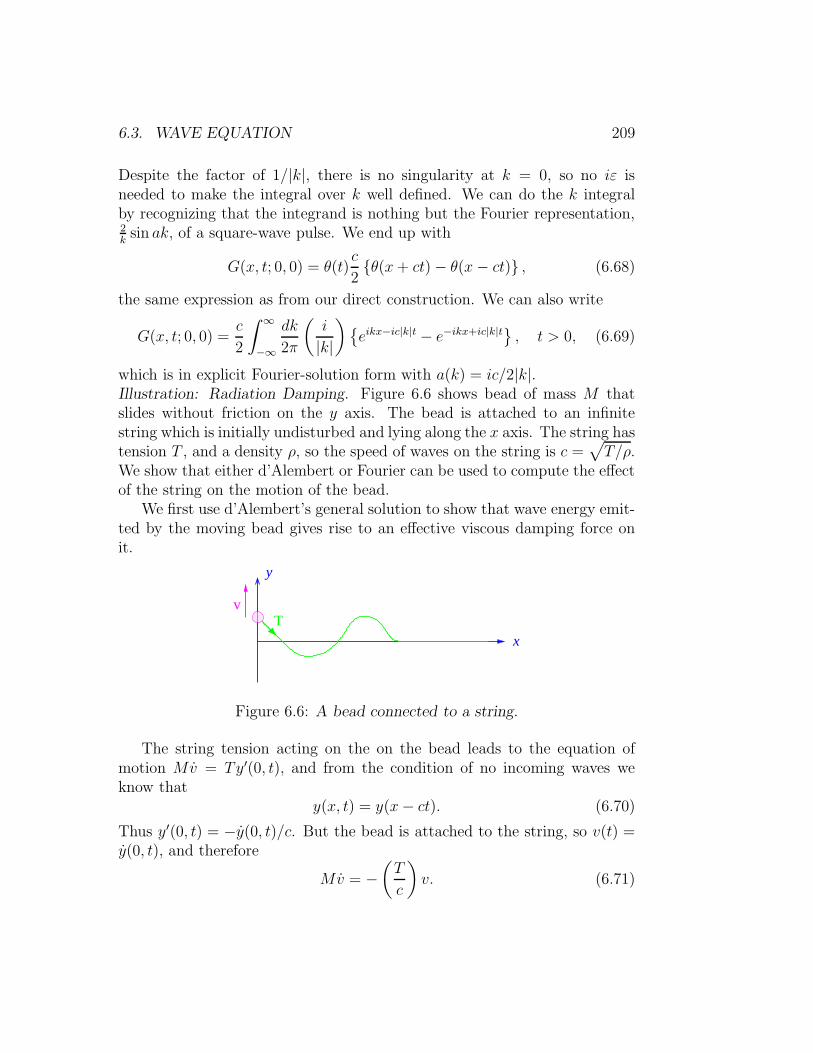
6.3. WAVE EQUATION 209
Despite the factor of 1/|k|, there is no singularity at k = 0, so no iε isneeded to make the integral over k well defined. We can do the k integralby recognizing that the integrand is nothing but the Fourier representation,2ksin ak, of a square-wave pulse. We end up with
G(x, t; 0, 0) = θ(t)c
2θ(x+ ct)− θ(x− ct) , (6.68)
the same expression as from our direct construction. We can also write
G(x, t; 0, 0) =c
2
∫ ∞
−∞
dk
2π
(i
|k|
)eikx−ic|k|t − e−ikx+ic|k|t
, t > 0, (6.69)
which is in explicit Fourier-solution form with a(k) = ic/2|k|.Illustration: Radiation Damping. Figure 6.6 shows bead of mass M thatslides without friction on the y axis. The bead is attached to an infinitestring which is initially undisturbed and lying along the x axis. The string hastension T , and a density ρ, so the speed of waves on the string is c =
√T/ρ.
We show that either d’Alembert or Fourier can be used to compute the effectof the string on the motion of the bead.
We first use d’Alembert’s general solution to show that wave energy emit-ted by the moving bead gives rise to an effective viscous damping force onit.
v
x
y
T
Figure 6.6: A bead connected to a string.
The string tension acting on the on the bead leads to the equation ofmotion Mv = Ty′(0, t), and from the condition of no incoming waves weknow that
y(x, t) = y(x− ct). (6.70)
Thus y′(0, t) = −y(0, t)/c. But the bead is attached to the string, so v(t) =y(0, t), and therefore
Mv = −(T
c
)v. (6.71)

210 CHAPTER 6. PARTIAL DIFFERENTIAL EQUATIONS
The emitted radiation therefore generates a velocity-dependent drag forcewith friction coefficient η = T/c.
We need an infinitely long string for (6.71) to be true for all time. Ifthe string had a finite length L, then, after a period of 2L/c, energy will bereflected back to the bead and this will complicate matters.
x
’(x)0
(x)0
φ
− φ1
Figure 6.7: The function φ0(x) and its derivative.
We now show that Fourier’s mode-decomposition of the string motion,combined with the Caldeira-Leggett analysis of chapter 5, yields the sameexpression for the radiation damping as the d’Alembert solution. Our bead-string contraption has Lagrangian
L =M
2[y(0, t)]2 − V [y(0, t)] +
∫ L
0
ρ
2y2 − T
2y′
2
dx. (6.72)
Here, V [y] is some potential energy for the bead.
To deal with the motion of the bead, we introduce a function φ0(x) suchthat φ0(0) = 1 and φ0(x) decreases rapidly to zero as x increases (see figure6.7. We therefore have −φ′
0(x) ≈ δ(x). We expand y(x, t) in terms of φ0(x)and the normal modes of a string with fixed ends as
y(x, t) = y(0, t)φ0(x) +∞∑
n=1
qn(t)
√2
Lρsin knx. (6.73)
Here knL = nπ. Because y(0, t)φ0(x) describes the motion of only an in-finitesimal length of string, y(0, t) makes a negligeable contribution to thestring kinetic energy, but it provides a linear coupling of the bead to thestring normal modes, qn(t), through the Ty′2/2 term. Inserting the mode

6.3. WAVE EQUATION 211
expansion into the Lagrangian, and after about half a page of arithmetic, weend up with
L =M
2[y(0)]2−V [y(0)]+y(0)
∞∑
n=1
fnqn+∞∑
n=1
(1
2q2n − ω2
nq2n
)−12
∞∑
n=1
(f 2n
ω2n
)y(0)2,
(6.74)where ωn = ckn, and
fn = T
√2
Lρkn. (6.75)
This is exactly the Caldeira-Leggett Lagrangian — including their frequency-shift counter-term that reflects that fact that a static displacement of aninfinite string results in no additional force on the bead.1 When L becomeslarge, the eigenvalue density of states
ρ(ω) =∑
n
δ(ω − ωn) (6.76)
becomes
ρ(ω) =L
πc. (6.77)
The Caldeira-Leggett spectral function
J(ω) =π
2
∑
n
(f 2n
ωn
)δ(ω − ωn), (6.78)
is therefore
J(ω) =π
2· 2T
2k2
Lρ· 1kc· Lπc
=
(T
c
)ω, (6.79)
where we have used c =√T/ρ. Comparing with Caldeira-Leggett’s J(ω) =
ηω, we see that the effective viscosity is given by η = T/c, as before. Thenecessity of having an infinitely long string here translates into the require-ment that we must have a continuum of oscillator modes. It is only after thesum over discrete modes ωi is replaced by an integral over the continuum ofω’s that no energy is ever returned to the system being damped.
1For a finite length of string that is fixed at the far end, the string tension does add12Ty(0)
2/L to the static potential. In the mode expansion, this additional restoring forcearises from the first term of−φ′0(x) ≈ 1/L+(2/L)
∑∞n=1 cos knx in 1
2Ty(0)2∫(φ′0)
2 dx. Thesubsequent terms provide the Caldeira-Leggett counter-term. The first-term contributionhas been omitted in (6.74) as being unimportant for large L.

212 CHAPTER 6. PARTIAL DIFFERENTIAL EQUATIONS
For our bead and string, the mode-expansion approach is more com-plicated than d’Alembert’s. In the important problem of the drag forcesinduced by the emission of radiation from an accelerated charged particle,however, the mode-expansion method leads to an informative resolution2 ofthe pathologies of the Abraham-Lorentz equation,
M(v − τ v) = Fext, τ =2
3
e2
Mc31
4πε0(6.80)
which is plagued by runaway, or apparently acausal, solutions.
6.3.4 Odd vs. Even Dimensions
Consider the wave equation for sound in the three dimensions. We have avelocity potential φ which obeys the wave equation
∂2φ
∂x2+∂2φ
∂y2+∂2φ
∂z2− 1
c2∂2φ
∂t2= 0, (6.81)
and from which the velocity, density, and pressure fluctuations can be ex-tracted as
v1 = ∇φ,ρ1 = −ρ0
c2φ,
P1 = c2ρ1. (6.82)
In three dimensions, and considering only spherically symmetric waves,the wave equation becomes
∂2(rφ)
∂r2− 1
c2∂2(rφ)
∂t2= 0, (6.83)
with solution
φ(r, t) =1
rf(t− r
c
)+
1
rg(t+
r
c
). (6.84)
Consider what happens if we put a point volume source at the origin (thesudden conversion of a negligeable volume of solid explosive to a large volume
2G. W. Ford, R. F. O’Connell, Phys. Lett. A 157 (1991) 217.

6.3. WAVE EQUATION 213
of hot gas, for example). Let the rate at which volume is being intruded beq. The gas velocity very close to the origin will be
v(r, t) =q(t)
4πr2. (6.85)
Matching this to an outgoing wave gives
q(t)
4πr2= v1(r, t) =
∂φ
∂r= − 1
r2f(t− r
c
)− 1
rcf ′(t− r
c
). (6.86)
Close to the origin, in the near field , the term ∝ f/r2 will dominate, and so
− 1
4πq(t) = f(t). (6.87)
Further away, in the far field or radiation field , only the second term willsurvive, and so
v1 =∂φ
∂r≈ − 1
rcf ′(t− r
c
). (6.88)
The far-field velocity-pulse profile v1 is therefore the derivative of the near-field v1 pulse profile.
v
x
Near field Far field
x
v or P
Figure 6.8: Three-dimensional blast wave.
The pressure pulse
P1 = −ρ0φ =ρ04πr
q(t− r
c
)(6.89)
is also of this form. Thus, a sudden localized expansion of gas produces anoutgoing pressure pulse which is first positive and then negative.

214 CHAPTER 6. PARTIAL DIFFERENTIAL EQUATIONS
This phenomenon can be seen in (old, we hope) news footage of bombblasts in tropical regions. A spherical vapour condensation wave can beenseen spreading out from the explosion. The condensation cloud is caused bythe air cooling below the dew-point in the low-pressure region which tails theover-pressure blast.
Now consider what happens if we have a sheet of explosive, the simultane-ous detonation of every part of which gives us a one-dimensional plane-wavepulse. We can obtain the plane wave by adding up the individual sphericalwaves from each point on the sheet.
r
xs
P
Figure 6.9: Sheet-source geometry.
Using the notation defined in figure 6.9, we have
φ(x, t) = 2π
∫ ∞
0
1√x2 + s2
f
(t−√x2 + s2
c
)sds (6.90)
with f(t) = −q(t)/4π, where now q is the rate at which volume is beingintruded per unit area of the sheet. We can write this as
2π
∫ ∞
0
f
(t−√x2 + s2
c
)d√x2 + s2,
= 2πc
∫ t−x/c
−∞f(τ) dτ,

6.3. WAVE EQUATION 215
= − c2
∫ t−x/c
−∞q(τ) dτ. (6.91)
In the second line we have defined τ = t −√x2 + s2/c, which, inter alia,
interchanged the role of the upper and lower limits on the integral.Thus, v1 = φ′(x, t) = 1
2q(t − x/c). Since the near field motion produced
by the intruding gas is v1(r) =12q(t), the far-field displacement exactly re-
produces the initial motion, suitably delayed of course. (The factor 1/2 isbecause half the intruded volume goes towards producing a pulse in the neg-ative direction.)
In three dimensions, the far-field motion is the first derivative of the near-field motion. In one dimension, the far-field motion is exactly the same asthe near-field motion. In two dimensions the far-field motion should there-fore be the half-derivative of the near-field motion — but how do you half-differentiate a function? An answer is suggested by the theory of Laplacetransformations as
(d
dt
) 12
F (t)def=
1√π
∫ t
−∞
F (τ)√t− τ dτ. (6.92)
Let us now repeat the explosive sheet calculation for an exploding wire.
sr
Px
Figure 6.10: Line-source geometry.
Using the geometry shown in figure 6.10, we have
ds = d(√
r2 − x2)=
r dr√r2 − x2
, (6.93)

216 CHAPTER 6. PARTIAL DIFFERENTIAL EQUATIONS
and combining the contributions of the two parts of the wire that are thesame distance from p, we can write
φ(x, t) =
∫ ∞
x
1
rf(t− r
c
) 2r dr√r2 − x2
= 2
∫ ∞
x
f(t− r
c
) dr√r2 − x2
, (6.94)
with f(t) = −q(t)/4π, where now q is the volume intruded per unit length.We may approximate r2−x2 ≈ 2x(r−x) for the near parts of the wire wherer ≈ x, since these make the dominant contribution to the integral. We alsoset τ = t− r/c, and then have
φ(x, t) =2c√2x
∫ (t−x/c)
−∞f (τ)
dr√(ct− x)− cτ
,
= − 1
2π
√2c
x
∫ (t−x/c)
−∞q (τ)
dτ√(t− x/c)− τ
. (6.95)
The far-field velocity is the x gradient of this,
v1(r, t) =1
2πc
√2c
x
∫ (t−x/c)
−∞q (τ)
dτ√(t− x/c)− τ
, (6.96)
and is therefore proportional to the 1/2-derivative of q(t− r/c).
Near field Far field
v v
r r
Figure 6.11: In two dimensions the far-field pulse has a long tail.
A plot of near field and far field motions in figure 6.11 shows how thefar-field pulse never completely dies away to zero. This long tail means thatone cannot use digital signalling in two dimensions.
6.4. HEAT EQUATION 217
Moral Tale: One of our colleagues was performing numerical work on earth-quake propagation. The source of his waves was a long deep linear fault,so he used the two-dimensional wave equation. Not wanting to be troubledby the actual creation of the wave pulse, he took as initial data an outgoingfinite-width pulse. After a short propagation time his numerical solution ap-peared to misbehave. New pulses were being emitted from the fault long afterthe initial one. He wasted several months in vain attempt to improve thestability of his code before he realized that what he was seeing was real. Thelack of a long tail on his pulse meant that it could not have been created bya briefly-active line source. The new “unphysical” waves were a consequenceof the source striving to suppress the long tail of the initial pulse. Moral :Always check that a solution of the form you seek actually exists before youwaste your time trying to compute it.
Exercise 6.4: Use the calculus of improper integrals to show that, providedF (−∞) = 0, we have
d
dt
(1√π
∫ t
−∞
F (τ)√t− τ dτ
)=
1√π
∫ t
−∞
F (τ)√t− τ dτ. (6.97)
This means thatd
dt
(d
dt
) 12
F (t) =
(d
dt
)12 d
dtF (t). (6.98)
6.4 Heat Equation
Fourier’s heat equation∂φ
∂t= κ
∂2φ
∂x2(6.99)
is the archetypal parabolic equation. It often comes with initial data φ(x, t = 0),but this is not Cauchy data, as the curve t = const. is a characteristic.
The heat equation is also known as the diffusion equation.
6.4.1 Heat Kernel
If we Fourier transform the initial data
φ(x, t = 0) =
∫ ∞
−∞
dk
2πφ(k)eikx, (6.100)

218 CHAPTER 6. PARTIAL DIFFERENTIAL EQUATIONS
and write
φ(x, t) =
∫ ∞
−∞
dk
2πφ(k, t)eikx, (6.101)
we can plug this into the heat equation and find that
∂φ
∂t= −κk2φ. (6.102)
Hence,
φ(x, t) =
∫ ∞
−∞
dk
2πφ(k, t)eikx
=
∫ ∞
−∞
dk
2πφ(k, 0)eikx−κk
2t. (6.103)
We may now express φ(k, 0) in terms of φ(x, 0) and rearrange the order ofintegration to get
φ(x, t) =
∫ ∞
−∞
dk
2π
(∫ ∞
−∞φ(ξ, 0)eikξ dξ
)eikx−κk
2t
=
∫ ∞
−∞
(∫ ∞
−∞
dk
2πeik(x−ξ)−κk
2t
)φ(ξ, 0)dξ
=
∫ ∞
−∞G(x, ξ, t)φ(ξ, 0) dξ, (6.104)
where
G(x, ξ, t) =
∫ ∞
−∞
dk
2πeik(x−ξ)−κk
2t =1√4πκt
exp
− 1
4κt(x− ξ)2
. (6.105)
Here, G(x, ξ, t) is the heat kernel . It represents the spreading of a unit blobof heat.

6.4. HEAT EQUATION 219
G(x,ξ ,t)
ξx
Figure 6.12: The heat kernel at three successive times.
As the heat spreads, the total amount of heat, represented by the areaunder the curve in figure 6.12, remains constant:
∫ ∞
−∞
1√4πκt
exp
− 1
4κt(x− ξ)2
dx = 1. (6.106)
The heat kernel possesses a semigroup property
G(x, ξ, t1 + t2) =
∫ ∞
−∞G(x, η, t2)G(η, ξ, t1)dη. (6.107)
Exercise: Prove this.
6.4.2 Causal Green Function
Now we consider the inhomogeneous heat equation
∂u
∂t− ∂2u
∂x2= q(x, t), (6.108)
with initial data u(x, 0) = u0(x). We define a Causal Green function by
(∂
∂t− ∂2
∂x2
)G(x, t; ξ, τ) = δ(x− ξ)δ(t− τ) (6.109)

220 CHAPTER 6. PARTIAL DIFFERENTIAL EQUATIONS
and the requirement that G(x, t; ξ, τ) = 0 if t < τ . Integrating the equationfrom t = τ − ε to t = τ + ε tells us that
G(x, τ + ε; ξ, τ) = δ(x− ξ). (6.110)
Taking this delta function as initial data φ(x, t = τ) and inserting into (6.104)we read off
G(x, t; ξ, τ) = θ(t− τ) 1√4π(t− τ)
exp
− 1
4(t− τ)(x− ξ)2
. (6.111)
We apply this Green function to the solution of a problem involving botha heat source and initial data given at t = 0 on the entire real line. Weexploit a variant of the Lagrange-identity method we used for solving one-dimensional ODE’s with inhomogeneous boundary conditions. Let
Dx,t ≡∂
∂t− ∂2
∂x2, (6.112)
and observe that its formal adjoint,
D†x,t ≡ −
∂
∂t− ∂2
∂x2. (6.113)
is a “backward” heat-equation operator. The corresponding “backward”Green function
G†(x, t; ξ, τ) = θ(τ − t) 1√4π(τ − t)
exp
− 1
4(τ − t)(x− ξ)2
(6.114)
obeysD†x,tG
†(x, t; ξ, τ) = δ(x− ξ)δ(t− τ), (6.115)
with adjoint boundary conditions. These makeG† anti-causal , in thatG†(t− τ)vanishes when t > τ . Now we make use of the two-dimensional Lagrangeidentity
∫ ∞
−∞dx
∫ T
0
dtu(x, t)D†
x,tG†(x, t; ξ, τ)−
(Dx,tu(x, t)
)G†(x, t; ξ, τ)
=
∫ ∞
−∞dxu(x, 0)G†(x, 0; ξ, τ)
−∫ ∞
−∞dxu(x, T )G†(x, T ; ξ, τ)
. (6.116)

6.4. HEAT EQUATION 221
Assume that (ξ, τ) lies within the region of integration. Then the left handside is equal to
u(ξ, τ)−∫ ∞
−∞dx
∫ T
0
dtq(x, t)G†(x, t; ξ, τ)
. (6.117)
On the right hand side, the second integral vanishes because G† is zero ont = T . Thus,
u(ξ, τ) =
∫ ∞
−∞dx
∫ T
0
dtq(x, t)G†(x, t; ξ, τ)
+
∫ ∞
−∞
u(x, 0)G†(x, 0; ξ, τ)
dx
(6.118)Rewriting this by using
G†(x, t; ξ, τ) = G(ξ, τ ; x, t), (6.119)
and relabeling x↔ ξ and t↔ τ , we have
u(x, t) =
∫ ∞
−∞G(x, t; ξ, 0)u0(ξ) dξ +
∫ ∞
−∞
∫ t
0
G(x, t; ξ, τ)q(ξ, τ)dξdτ. (6.120)
Note how the effects of any heat source q(x, t) active prior to the initial-dataepoch at t = 0 have been subsumed into the evolution of the initial data.
6.4.3 Duhamel’s Principle
Often, the temperature of the spatial boundary of a region is specified inaddition to the initial data. Dealing with this type of problem leads us to anew strategy.
Suppose we are required to solve
∂u
∂t= κ
∂2u
∂x2(6.121)
for the semi-infinite rod shown in figure 6.13. We are given a specified tem-perature, u(0, t) = h(t), at the end x = 0, and for all other points x > 0 weare given an initial condition u(x, 0) = 0.

222 CHAPTER 6. PARTIAL DIFFERENTIAL EQUATIONS
x
h(t)
u(x,t)
u
Figure 6.13: Semi-infinite rod heated at one end.
We begin by finding a solution w(x, t) that satisfies the heat equation withw(0, t) = 1 and initial data w(x, 0) = 0, x > 0. This solution is constructedin problem 6.14, and is
w = θ(t)
1− erf
(x
2√t
). (6.122)
Here erf(x) is the error function
erf(x) =2√π
∫ x
0
e−z2
dz. (6.123)
which has the properties that erf(0) = 0 and erf(x) → 1 as x → ∞. Seefigure 6.14.
1
x
erf(x)
Figure 6.14: Error function.
If we were givenh(t) = h0θ(t− t0), (6.124)
then the desired solution would be
u(x, t) = h0w(x, t− t0). (6.125)
6.5. POTENTIAL THEORY 223
For a sum
h(t) =∑
n
hnθ(t− tn), (6.126)
the principle of superposition (i.e. the linearity of the problem) tell us thatthe solution is the corresponding sum
u(x, t) =∑
n
hnw(x, t− tn). (6.127)
We therefore decompose h(t) into a sum of step functions
h(t) = h(0) +
∫ t
0
h(τ) dτ
= h(0) +
∫ ∞
0
θ(t− τ)h(τ) dτ. (6.128)
It is should now be clear that
u(x, t) =
∫ t
0
w(x, t− τ)h(τ) dτ + h(0)w(x, t)
= −∫ t
0
(∂
∂τw(x, t− τ)
)h(τ) dτ
=
∫ t
0
(∂
∂tw(x, t− τ)
)h(τ) dτ. (6.129)
This is called Duhamel’s solution, and the trick of expressing the data as asum of Heaviside step functions is called Duhamel’s principle.
We do not need to be as clever as Duhamel. We could have obtainedthis result by using the method of images to find a suitable causal Greenfunction for the half line, and then using the same Lagrange-identity methodas before.
6.5 Potential Theory
The study of boundary-value problems involving the Laplacian is usuallyknown as “‘Potential Theory.” We seek solutions to these problems in someregion Ω, whose boundary we denote by the symbol ∂Ω.

224 CHAPTER 6. PARTIAL DIFFERENTIAL EQUATIONS
Poisson’s equation, −∇2χ(r) = f(r), r ∈ Ω, and the Laplace equation towhich it reduces when f(r) ≡ 0, come along with various boundary condi-tions, of which the commonest are
χ = g(r) on ∂Ω, (Dirichlet)
(n · ∇)χ = g(r) on ∂Ω. (Neumann) (6.130)
A function for which ∇2χ = 0 in some region Ω is said to be harmonic there.
6.5.1 Uniqueness and existence of solutions
We begin by observing that we need to be a little more precise about whatit means for a solution to “take” a given value on a boundary. If we ask fora solution to the problem ∇2ϕ = 0 within Ω = (x, y) ∈ R2 : x2 + y2 < 1and ϕ = 1 on ∂Ω, someone might claim that the function defined by settingϕ(x, y) = 0 for x2 + y2 < 1 and ϕ(x, y) = 1 for x2 + y2 = 1 does the job—but such a discontinuous “solution” is hardly what we had in mind when westated the problem. We must interpret the phrase “takes a given value on theboundary” as meaning that the boundary data is the limit, as we approachthe boundary, of the solution within Ω.
With this understanding, we assert that a function harmonic in a boundedsubset Ω of Rn is uniquely determined by the values it takes on the boundaryof Ω. To see that this is so, suppose that ϕ1 and ϕ2 both satisfy ∇2ϕ = 0 inΩ, and coincide on the boundary. Then χ = ϕ1 − ϕ2 obeys ∇2χ = 0 in Ω,and is zero on the boundary. Integrating by parts we find that
∫
Ω
|∇χ|2dnr =∫
∂Ω
χ(n · ∇)χ dS = 0. (6.131)
Here dS is the element of area on the boundary and n the outward-directednormal. Now, because the second derivatives exist, the partial derivativesentering into ∇χ must be continuous, and so the vanishing of integral of|∇χ|2 tells us that ∇χ is zero everywhere within Ω. This means that χ isconstant — and because it is zero on the boundary it is zero everywhere.
An almost identical argument shows that if Ω is a bounded connectedregion, and if ϕ1 and ϕ2 both satisfy ∇2ϕ = 0 within Ω and take the samevalues of (n ·∇)ϕ on the boundary, then ϕ1 = ϕ2+ const. We have thereforeshown that, if it exists, the solutions of the Dirichlet boundary value problem
6.5. POTENTIAL THEORY 225
is unique, and the solution of the Neumann problem is unique up to theaddition of an arbitrary constant.
In the Neumann case, with boundary condition (n · ∇)ϕ = g(r), andintegration by parts gives
∫
Ω
∇2ϕdnr =
∫
∂Ω
(n · ∇)ϕdS =
∫
∂Ω
g dS, (6.132)
and so the boundary data g(r) must satisfy∫∂Ωg dS = 0 if a solution to
∇2ϕ = 0 is to exist. This is an example of the Fredhom alternative thatrelates the existence of a non-trivial null space to constraints on the sourceterms. For the inhomogeneous equation −∇2ϕ = f , the Fredholm constraintbecomes ∫
∂Ω
g dS +
∫
Ω
f dnr = 0. (6.133)
Given that we have satisfied any Fredholm constraint, do solutions to theDirichlet and Neumann problem always exist? That solutions should exist issuggested by physics: the Dirichlet problem corresponds to an electrostaticproblem with specified boundary potentials and the Neumann problem cor-responds to finding the electric potential within a resistive material withprescribed current sources on the boundary. The Fredholm constraint saysthat if we drive current into the material, we must must let it out somewhere.Surely solutions always exist to these physics problems? In the Dirichlet casewe can even make a mathematically plausible argument for existence: Weobserve that the boundary-value problem
∇2ϕ = 0, r ∈ Ω
ϕ = f, r ∈ ∂Ω (6.134)
is solved by taking ϕ to be the χ that minimizes the functional
J [χ] =
∫
Ω
|∇χ|2dnr (6.135)
over the set of continuously differentiable functions taking the given boundaryvalues. Since J [χ] is positive, and hence bounded below, it seems intuitivelyobvious that there must be some function χ for which J [χ] is a minimum.The appeal of this Dirichlet principle argument led even Riemann astray.The fallacy was exposed by Weierstrass who provided counterexamples.

226 CHAPTER 6. PARTIAL DIFFERENTIAL EQUATIONS
Consider, for example, the problem of finding a function ϕ(x, y) obeying∇2ϕ = 0 within the punctured disc D′ = (x, y) ∈ R2 : 0 < x2 + y2 < 1with boundary data ϕ(x, y) = 1 on the outer boundary at x2 + y2 = 1 andϕ(0, 0) = 0 on the inner boundary at the origin. We substitute the trialfunctions
χα(x, y) = (x2 + y2)α, α > 0, (6.136)
all of which satisfy the boundary data, into the positive functional
J [χ] =
∫
D′
|∇χ|2 dxdy (6.137)
to find J [χα] = 2πα. This number can be made as small as we like, and sothe infimum of the functional J [χ] is zero. But if there is a minimizing ϕ,then J [ϕ] = 0 implies that ϕ is a constant, and a constant cannot satisfy theboundary conditions.
An analogous problem reveals itself in three dimensions when the bound-ary of Ω has a sharp re-entrant spike that is held at a different potential fromthe rest of the boundary. In this case we can again find a sequence of trialfunctions χ(r) for which J [χ] becomes arbitrarily small, but the sequence ofχ’s has no limit satisfying the boundary conditions. The physics argumentalso fails: if we tried to create a physical realization of this situation, theelectric field would become infinite near the spike, and the charge would leakoff and and thwart our attempts to establish the potential difference. Forreasonably smooth boundaries, however, a minimizing function does exist.
The Dirichlet-Poisson problem
−∇2ϕ(r) = f(r), r ∈ Ω,
ϕ(r) = g(r), r ∈ ∂Ω, (6.138)
and the Neumann-Poisson problem
−∇2ϕ(r) = f(r), x ∈ Ω,
(n · ∇)ϕ(r) = g(r), x ∈ ∂Ω
supplemented with the Fredholm constraint
∫
Ω
f dnr +
∫
∂Ω
g dS = 0 (6.139)

6.5. POTENTIAL THEORY 227
also have solutions when ∂Ω is reasonably smooth. For the Neumann-Poissonproblem, with the Fredholm constraint as stated, the region Ω must be con-nected, but its boundary need not be. For example, Ω can be the regionbetween two nested spherical shells.
Exercise 6.5: Why did we insist that the region Ω be connected in our dis-cussion of the Neumann problem? (Hint: how must we modify the Fredholmconstraint when Ω consists of two or more disconnected regions?)
Exercise 6.6: Neumann variational principles. Let Ω be a bounded and con-nected three-dimensional region with a smooth boundary. Given a function fdefined on Ω and such that
∫Ω f d
3r = 0, define the functional
J [χ] =
∫
Ω
1
2|∇χ|2 − χf
d3r.
Suppose that ϕ is a solution of the Neumann problem
−∇2ϕ(r) = f(r), r ∈ Ω,
(n · ∇)ϕ(r) = 0, r ∈ ∂Ω.
Show that
J [χ] = J [ϕ] +
∫
Ω
1
2|∇(χ−ϕ)|2 d3r ≥ J [ϕ] = −
∫
Ω
1
2|∇ϕ|2 d3r = −1
2
∫
Ωϕf d3r.
Deduce that ϕ is determined, up to the addition of a constant, as the functionthat minimizes J [χ] over the space of all continuously differentiable χ (andnot just over functions satisfying the Neumann boundary condition.)
Similarly, for g a function defined on the boundary ∂Ω and such that∫∂Ω g dS =
0, set
K[χ] =
∫
Ω
1
2|∇χ|2 d3r −
∫
∂Ωχg dS.
Now suppose that φ is a solution of the Neumann problem
−∇2φ(r) = 0, r ∈ Ω,
(n · ∇)φ(r) = g(r), r ∈ ∂Ω.
Show that
K[χ] = K[φ]+
∫
Ω
1
2|∇(χ−φ)|2 d3r ≥ K[φ] = −
∫
Ω
1
2|∇φ|2 d3r = −1
2
∫
∂Ωφg dS.
228 CHAPTER 6. PARTIAL DIFFERENTIAL EQUATIONS
Deduce that φ is determined up to a constant as the function that minimizesK[χ] over the space of all continuously differentiable χ (and, again, not justover functions satisfying the Neumann boundary condition.)
Show that when f and g fail to satisfy the integral conditions required forthe existence of the Neumann solution, the corresponding functionals are notbounded below, and so no minimizing function can exist.
Exercise 6.7: Helmholtz decomposition Let Ω be a bounded connected three-dimensional region with smooth boundary ∂Ω.
a) Cite the conditions for the existence of a solution to a suitable Neumannproblem to show that if u is a smooth vector field defined in Ω, thenthere exist a unique solenoidal (i.e having zero divergence) vector fieldv with v · n = 0 on the boundary ∂Ω, and a unique (up to the additionof a constant) scalar field φ such that
u = v +∇φ.Here n is the outward normal to the (assumed smooth) bounding surfaceof Ω.
b) In many cases (but not always) we can write a solenoidal vector field v
as v = curlw. Again by appealing to the conditions for existence anduniqueness of a Neumann problem solution, show that if we can writev = curlw, then w is not unique, and we can always demand that itobey the conditions divw = 0 and w · n = 0.
c) Appeal to the Helmholtz decomposition of part a) with u→ (v · ∇)v toshow that in the Euler equation
∂v
∂t+ (v · ∇)v = −∇P, v · n = 0 on ∂Ω
governing the motion of an incompressible (divv = 0) fluid the instan-taneous flow field v(x, y, z, t) uniquely determines ∂v/∂t, and hence thetime evolution of the flow. (This observation provides the basis of prac-tical algorithms for computing incompressible flows.)
We can always write the solenoidal field as v = curlw + h, where h obeys∇2h = 0 with suitable boundary conditions. See exercise 6.16.
6.5.2 Separation of Variables
Cartesian Coordinates
When the region of interest is a square or a rectangle, we can solve Laplaceboundary problems by separating the Laplace operator in cartesian co-ordinates.

6.5. POTENTIAL THEORY 229
Let
∂2ϕ
∂x2+∂2ϕ
∂y2= 0, (6.140)
and write
ϕ = X(x)Y (y), (6.141)
so that
1
X
∂2X
∂x2+
1
Y
∂2Y
∂y2= 0. (6.142)
Since the first term is a function of x only, and the second of y only, bothmust be constants and the sum of these constants must be zero. Therefore
1
X
∂2X
∂x2= −k2,
1
Y
∂2Y
∂y2= k2, (6.143)
or, equivalently
∂2X
∂x2+ k2X = 0,
∂2Y
∂y2− k2Y = 0. (6.144)
The number that we have, for later convenience, written as k2 is called aseparation constant . The solutions are X = e±ikx and Y = e±ky. Thus
ϕ = e±ikxe±ky, (6.145)
or a sum of such terms where the allowed k’s are determined by the boundaryconditions.
How do we know that the separated form X(x)Y (y) captures all possiblesolutions? We can be confident that we have them all if we can use the sep-arated solutions to solve boundary-value problems with arbitrary boundarydata.

230 CHAPTER 6. PARTIAL DIFFERENTIAL EQUATIONS
L
x
y
L
Figure 6.15: Square region.
We can use our separated solutions to construct the unique harmonicfunction taking given values on the sides a square of side L shown in figure6.15. To see how to do this, consider the four families of functions
ϕ1,n =
√2
L
1
sinh nπsin
nπx
Lsinh
nπy
L,
ϕ2,n =
√2
L
1
sinh nπsinh
nπx
Lsin
nπy
L,
ϕ3,n =
√2
L
1
sinh nπsin
nπx
Lsinh
nπ(L− y)L
,
ϕ4,n =
√2
L
1
sinh nπsinh
nπ(L− x)L
sinnπy
L. (6.146)
Each of these comprises solutions to ∇2ϕ = 0. The family ϕ1,n(x, y) has beenconstructed so that every member is zero on three sides of the square, buton the side y = L it becomes ϕ1,n(x, L) =
√2/L sin(nπx/L). The ϕ1,n(x, L)
therefore constitute an complete orthonormal set in terms of which we canexpand the boundary data on the side y = L. Similarly, the other otherfamilies are non-zero on only one side, and are complete there. Thus, anyboundary data can be expanded in terms of these four function sets, and thesolution to the boundary value problem is given by a sum
ϕ(x, y) =
4∑
m=1
∞∑
n=1
am,nϕm,n(x, y). (6.147)

6.5. POTENTIAL THEORY 231
The solution to ∇2ϕ = 0 in the unit square with ϕ = 1 on the side y = 1and zero on the other sides is, for example,
ϕ(x, y) =∞∑
n=0
4
(2n+ 1)π
1
sinh(2n + 1)πsin((2n+ 1)πx
)sinh
((2n+ 1)πy
)
(6.148)
00.2
0.4
0.6
0.8
1 0
0.2
0.4
0.6
0.8
1
00.250.5
0.751
00.2
0.4
0.6
0.8
1
Figure 6.16: Plot of first thiry terms in equation (6.148).
For cubes, and higher dimensional hypercubes, we can use similar bound-ary expansions. For the unit cube in three dimensions we would use
ϕ1,nm(x, y, x) =1
sinh(π√n2 +m2
) sin(nπx) sin(mπy) sinh(πz√n2 +m2
),
to expand the data on the face z = 1, together with five other solutionfamilies, one for each of the other five faces of the cube.
If some of the boundaries are at infinity, we may need only need some ofthese functions.
Example: Figure 6.17 shows three conducting sheets, each infinite in the zdirection. The central one has width a, and is held at voltage V0. The outertwo extend to infinity also in the y direction, and are grounded. The resultingpotential should tend to zero as |x|, |y| → ∞.

232 CHAPTER 6. PARTIAL DIFFERENTIAL EQUATIONS
V0
x
y
z
a
O
Figure 6.17: Conducting sheets.
The voltage in the x = 0 plane is
ϕ(0, y, z) =
∫ ∞
−∞
dk
2πa(k)e−iky, (6.149)
where
a(k) = V0
∫ a/2
−a/2eiky dy =
2V0k
sin(ka/2). (6.150)
Then, taking into account the boundary condition at large x, the solution to∇2ϕ = 0 is
ϕ(x, y, z) =
∫ ∞
−∞
dk
2πa(k)e−ikye−|k||x|. (6.151)
The evaluation of this integral, and finding the charge distribution on thesheets, is left as an exercise.
The Cauchy Problem is Ill-posed
Although the Laplace equation has no characteristics, the Cauchy data prob-lem is ill-posed , meaning that the solution is not a continuous function of thedata. To see this, suppose we are given ∇2ϕ = 0 with Cauchy data on y = 0:
ϕ(x, 0) = 0,
∂ϕ
∂y
∣∣∣∣y=0
= ε sin kx. (6.152)

6.5. POTENTIAL THEORY 233
Thenϕ(x, y) =
ε
ksin(kx) sinh(ky). (6.153)
Provided k is large enough — even if ε is tiny — the exponential growth of thehyperbolic sine will make this arbitrarily large. Any infinitesimal uncertaintyin the high frequency part of the initial data will be vastly amplified, andthe solution, although formally correct, is useless in practice.
Polar coordinates
We can use the separation of variables method in polar coordinates. Here,
∇2χ =∂2χ
∂r2+
1
r
∂χ
∂r+
1
r2∂2χ
∂θ2. (6.154)
Setχ(r, θ) = R(r)Θ(θ). (6.155)
Then ∇2χ = 0 implies
0 =r2
R
(∂2R
∂r2+
1
r
∂R
∂r
)+
1
Θ
∂2Θ
∂θ2
= m2 − m2, (6.156)
where in the second line we have written the separation constant as m2.Therefore,
d2Θ
dθ2+m2Θ = 0, (6.157)
implying that Θ = eimθ, where m must be an integer if Θ is to be single-valued, and
r2d2R
dr2+ r
dR
dr−m2R = 0, (6.158)
whose solutions are R = r±m when m 6= 0, and 1 or ln r when m = 0. Thegeneral solution is therefore a sum of these
χ = A0 +B0 ln r +∑
m6=0
(Amr|m| +Bmr
−|m|)eimθ. (6.159)
The singular terms, ln r and r−|m|, are not solutions at the origin, and shouldbe omitted when that point is part of the region where ∇2χ = 0.
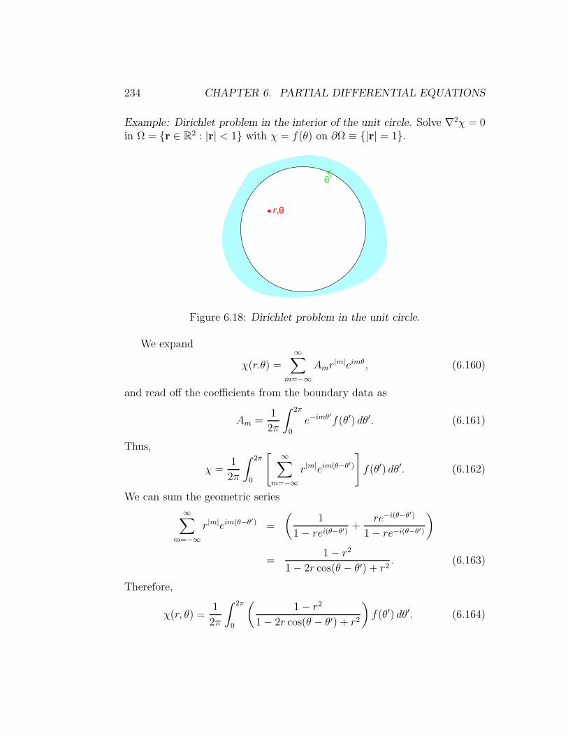
234 CHAPTER 6. PARTIAL DIFFERENTIAL EQUATIONS
Example: Dirichlet problem in the interior of the unit circle. Solve ∇2χ = 0in Ω = r ∈ R2 : |r| < 1 with χ = f(θ) on ∂Ω ≡ |r| = 1.
r,θ
θ’
Figure 6.18: Dirichlet problem in the unit circle.
We expand
χ(r.θ) =∞∑
m=−∞Amr
|m|eimθ, (6.160)
and read off the coefficients from the boundary data as
Am =1
2π
∫ 2π
0
e−imθ′
f(θ′) dθ′. (6.161)
Thus,
χ =1
2π
∫ 2π
0
[ ∞∑
m=−∞r|m|eim(θ−θ′)
]f(θ′) dθ′. (6.162)
We can sum the geometric series
∞∑
m=−∞r|m|eim(θ−θ′) =
(1
1− rei(θ−θ′) +re−i(θ−θ
′)
1− re−i(θ−θ′))
=1− r2
1− 2r cos(θ − θ′) + r2. (6.163)
Therefore,
χ(r, θ) =1
2π
∫ 2π
0
(1− r2
1− 2r cos(θ − θ′) + r2
)f(θ′) dθ′. (6.164)
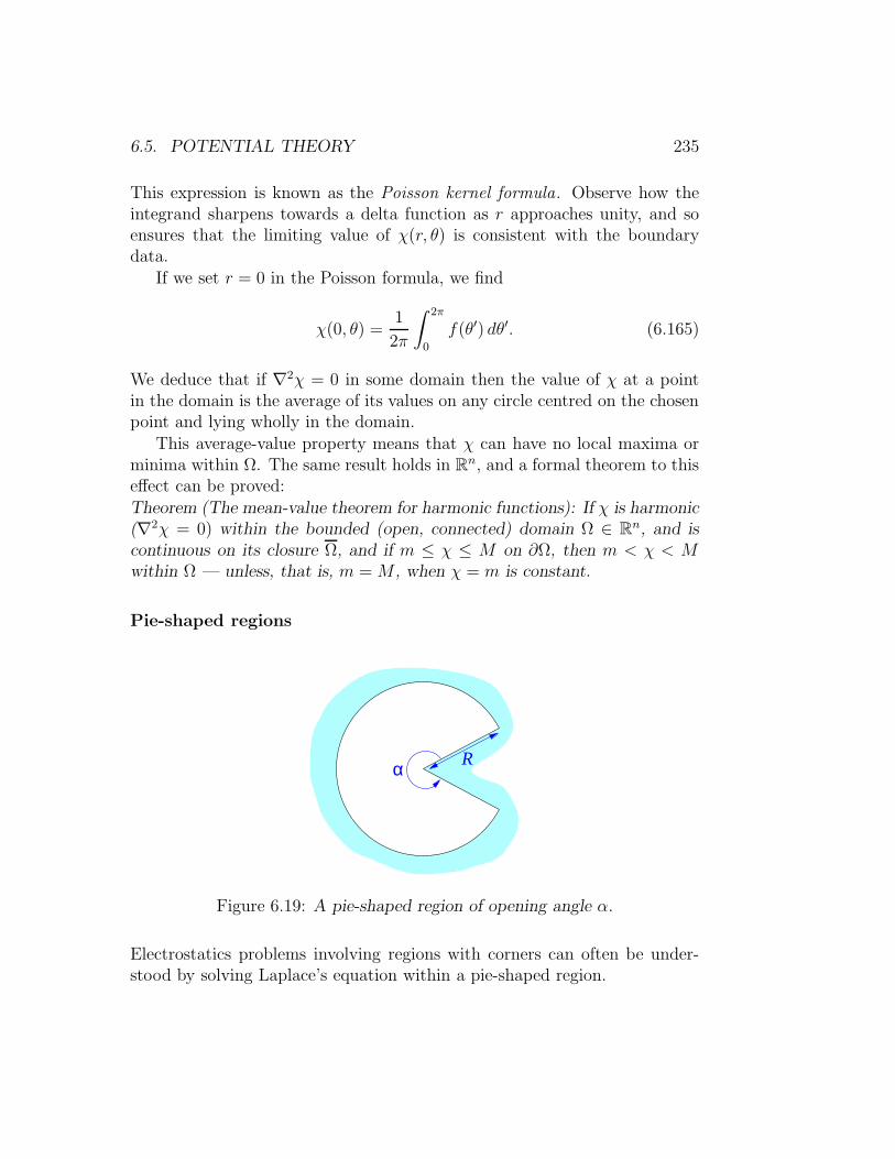
6.5. POTENTIAL THEORY 235
This expression is known as the Poisson kernel formula. Observe how theintegrand sharpens towards a delta function as r approaches unity, and soensures that the limiting value of χ(r, θ) is consistent with the boundarydata.
If we set r = 0 in the Poisson formula, we find
χ(0, θ) =1
2π
∫ 2π
0
f(θ′) dθ′. (6.165)
We deduce that if ∇2χ = 0 in some domain then the value of χ at a pointin the domain is the average of its values on any circle centred on the chosenpoint and lying wholly in the domain.
This average-value property means that χ can have no local maxima orminima within Ω. The same result holds in Rn, and a formal theorem to thiseffect can be proved:Theorem (The mean-value theorem for harmonic functions): If χ is harmonic(∇2χ = 0) within the bounded (open, connected) domain Ω ∈ Rn, and iscontinuous on its closure Ω, and if m ≤ χ ≤ M on ∂Ω, then m < χ < Mwithin Ω — unless, that is, m =M , when χ = m is constant.
Pie-shaped regions
α R
Figure 6.19: A pie-shaped region of opening angle α.
Electrostatics problems involving regions with corners can often be under-stood by solving Laplace’s equation within a pie-shaped region.

236 CHAPTER 6. PARTIAL DIFFERENTIAL EQUATIONS
Figure 6.19 shows a pie-shaped region of opening angle α and radius R.If the boundary value of the potential is zero on the wedge and non-zero onthe boundary arc, we can seek solutions as a sum of r, θ separated terms
ϕ(r, θ) =
∞∑
n=1
anrnπ/α sin
(nπθ
α
). (6.166)
Here the trigonometric function is not 2π periodic, but instead has beenconstructed so as to make ϕ vanish at θ = 0 and θ = α. These solutionsshow that close to the edge of a conducting wedge of external opening angleα, the surface charge density σ usually varies as σ(r) ∝ rα/π−1.
If we have non-zero boundary data on the edge of the wedge at θ = α,but have ϕ = 0 on the edge at θ = 0 and on the curved arc r = R, then thesolutions can be expressed as a continuous sum of r, θ separated terms
ϕ(r, θ) =1
2i
∫ ∞
0
a(ν)
(( rR
)iν−( rR
)−iν) sinh(νθ)
sinh(να)dν,
=
∫ ∞
0
a(ν) sin[ν ln(r/R)]sinh(νθ)
sinh(να)dν. (6.167)
The Mellin sine transformation can be used to computing the coefficientfunction a(ν). This transformation lets us write
f(r) =2
π
∫ ∞
0
F (ν) sin(ν ln r) dν, 0 < r < 1, (6.168)
where
F (ν) =
∫ 1
0
sin(ν ln r)f(r)dr
r. (6.169)
The Mellin sine transformation is a disguised version of the Fourier sinetransform of functions on [0,∞). We simply map the positive x axis ontothe interval (0, 1] by the change of variables x = − ln r.
Despite its complexity when expressed in terms of these formulae, thesimple solution ϕ(r, θ) = aθ is often the physically relevant one when the twosides of the wedge are held at different potentials and the potential is allowedto vary on the curved arc.Example: Consider a pie-shaped region of opening angle π and radius R =∞. This region can be considered to be the upper half-plane. Suppose thatwe are told that the positive x axis is held at potential +1/2 and the negative

6.5. POTENTIAL THEORY 237
x axis is at potential −1/2, and are required to find the potential for positivey. If we separate Laplace’s equation in cartesian co-ordinates and match tothe boundary data on the x-axes, we end up with
ϕxy(x, y) =1
π
∫ ∞
0
1
ke−ky sin(kx) dk.
On the other hand, the function
ϕrθ(r, θ) =1
π(π/2− θ)
satisfies both Laplace’s equation and the boundary data. At this point weought to worry that we do not have enough data to determine the solutionuniquely — nothing was said in the statement of the problem about thebehavior of ϕ on the boundary arc at infinity — but a little effort shows that
1
π
∫ ∞
0
1
ke−ky sin(kx) dk =
1
πtan−1
(x
y
), y > 0,
=1
π(π/2− θ),
(6.170)
and so the two expressions for ϕ(x, y) are equal.
6.5.3 Eigenfunction Expansions
Elliptic operators are the natural analogues of the one-dimensional lineardifferential operators we studied in earlier chapters.
The operator L = −∇2 is formally self-adjoint with respect to the innerproduct
〈φ, χ〉 =∫∫
φ∗χ dxdy. (6.171)
This property follows from Green’s identity
∫∫
Ω
φ∗(−∇2χ)− (−∇2φ)∗χ
dxdy =
∫
∂Ω
φ∗(−∇χ)− (−∇φ)∗χ · nds(6.172)
where ∂Ω is the boundary of the region Ω and n is the outward normal onthe boundary.
238 CHAPTER 6. PARTIAL DIFFERENTIAL EQUATIONS
The method of separation of variables also allows us to solve eigenvalueproblems involving the Laplace operator. For example, the Dirichlet eigen-value problem requires us to find the eigenfunctions and eigenvalues of theoperator
L = −∇2, D(L) = φ ∈ L2[Ω] : φ = 0, on ∂Ω. (6.173)
Suppose Ω is the rectangle 0 ≤ x ≤ Lx, 0 ≤ y ≤ Ly. The normalizedeigenfunctions are
φn,m(x, y) =
√4
LxLysin
(nπx
Lx
)sin
(mπy
Ly
), (6.174)
with eigenvalues
λn,m =
(n2π2
L2x
)+
(m2π2
L2y
). (6.175)
The eigenfunctions are orthonormal,
∫φn,mφn′,m′ dxdy = δnn′δmm′ , (6.176)
and complete. Thus, any function in L2[Ω] can be expanded as
f(x, y) =
∞∑
m,n=1
Anmφn,m(x, y), (6.177)
where
Anm =
∫∫φn,m(x, y)f(x, y) dxdy. (6.178)
We can find a complete set of eigenfunctions in product form whenever wecan separate the Laplace operator in a system of co-ordinates ξi such that theboundary becomes ξi = const. Completeness in the multidimensional spaceis then guaranteed by the completeness of the eigenfunctions of each one-dimensional differential operator. For other than rectangular co-ordinates,however, the separated eigenfunctions are not elementary functions.
The Laplacian has a complete set of Dirichlet eigenfunctions in any region,but in general these eigenfunctions cannot be written as separated productsof one-dimensional functions.

6.5. POTENTIAL THEORY 239
6.5.4 Green Functions
Once we know the eigenfunctions ϕn and eigenvalues λn for −∇2 in a regionΩ, we can write down the Green function as
g(r, r′) =∑
n
1
λnϕn(r)ϕ
∗n(r
′).
For example, the Green function for the Laplacian in the entire Rn is givenby the sum over eigenfunctions
g(r, r′) =
∫dnk
(2π)neik·(r−r′)
k2. (6.179)
Thus
−∇2rg(r, r
′) =
∫dnk
(2π)neik·(r−r′) = δn(r− r′). (6.180)
We can evaluate the integral for any n by using Schwinger’s trick to turn theintegrand into a Gaussian:
g(r, r′) =
∫ ∞
0
ds
∫dnk
(2π)neik·(r−r′)e−sk
2
=
∫ ∞
0
ds
(√π
s
)n1
(2π)ne−
14s
|r−r′|2
=1
2nπn/2
∫ ∞
0
dt tn2−2e−t|r−r′|2/4
=1
2nπn/2Γ(n2− 1)( |r− r′|2
4
)1−n/2
=1
(n− 2)Sn−1
(1
|r− r′|
)n−2
. (6.181)
Here, Γ(x) is Euler’s gamma function:
Γ(x) =
∫ ∞
0
dt tx−1e−t, (6.182)
and
Sn−1 =2πn/2
Γ(n/2)(6.183)

240 CHAPTER 6. PARTIAL DIFFERENTIAL EQUATIONS
is the surface area of the n-dimensional unit ball.For three dimensions we find
g(r, r′) =1
4π
1
|r− r′| , n = 3. (6.184)
In two dimensions the Fourier integral is divergent for small k. We maycontrol this divergence by using dimensional regularization. We pretend thatn is a continuous variable and use
Γ(x) =1
xΓ(x+ 1) (6.185)
together withax = ea lnx = 1 + a lnx+ · · · (6.186)
to to examine the behaviour of g(r, r′) near n = 2:
g(r, r′) =1
4π
Γ(n/2)
(n/2− 1)
(1− (n/2− 1) ln(π|r− r′|2) +O
[(n− 2)2
])
=1
4π
(1
n/2− 1− 2 ln |r− r′| − ln π − γ + · · ·
). (6.187)
Here γ = −Γ′(1) = .57721 . . . is the Euler-Mascheroni constant. Althoughthe pole 1/(n−2) blows up at n = 2, it is independent of position. We simplyabsorb it, and the − ln π− γ, into an undetermined additive constant. Oncewe have done this, the limit n→ 2 can be taken and we find
g(r, r′) = − 1
2πln |r− r′|+ const., n = 2. (6.188)
The constant does not affect the Green-function property, so we can choseany convenient value for it.
Although we have managed to sweep the small-k divergence of the Fourierintegral under a rug, the hidden infinity still has the capacity to cause prob-lems. The Green function in R3 allows us to to solve for ϕ(r) in the equation
−∇2ϕ = q(r),
with the boundary condition ϕ(r)→ 0 as |r| → ∞, as
ϕ(r) =
∫g(r, r′)q(r′) d3r.

6.5. POTENTIAL THEORY 241
In two dimensions, however we try to adjust the arbitrary constant in (6.188),the divergence of the logarithm at infinity means that there can be no solutionto the corresponding boundary-value problem unless
∫q(r) d3r = 0. This is
not a Fredholm-alternative constraint because once the constraint is satisfiedthe solution is unique. The two-dimensional problem is therefore patholog-ical from the viewpoint of Fredholm theory. This pathology is of the samecharacter as the non-existence of solutions to the three-dimensional Dirichletboundary-value problem with boundary spikes. The Fredholm alternativeapplies, in general, only to operators a discrete spectrum.
Exercise 6.8: Evaluate our formula for the Rn Laplace Green function,
g(r, r′) =1
(n− 2)Sn−1|r− r′|n−2
with Sn−1 = 2πn/2/Γ(n/2), for the case n = 1. Show that the resultingexpression for g(x, x′) is not divergent, and obeys
− d2
dx2g(x, x′) = δ(x− x′).
Our formula therefore makes sense as a Green function — even though theoriginal integral (6.179) is linearly divergent at k = 0! We must defer anexplanation of this miracle until we discuss analytic continuation in the contextof complex analysis.(Hint: recall that Γ(1/2) =
√π)
6.5.5 Boundary-value problems
We now look at how the Green function can be used to solve the interiorDirichlet boundary-value problem in regions where the method of separationof variables is not available. Figure 6.20 shows a bounded region Ω possessinga smooth boundary ∂Ω.

242 CHAPTER 6. PARTIAL DIFFERENTIAL EQUATIONS
Ω
r’r
n
Figure 6.20: Interior Dirichlet problem.
We wish to solve −∇2ϕ = q(r) for r ∈ Ω and with ϕ(r) = f(r) for r ∈ ∂Ω.Suppose we have found a Green function that obeys
−∇2rg(r, r
′) = δn(r− r′), r, r′ ∈ Ω, g(r, r′) = 0, r ∈ ∂Ω. (6.189)
We first show that g(r, r′) = g(r′, r) by the same methods we used for one-dimensional self-adjoint operators. Next we follow the strategy that we usedfor one-dimensional inhomogeneous differential equations: we use Lagrange’sidentity (in this context called Green’s theorem) to write
∫
Ω
dnrg(r, r′)∇2
rϕ(r)− ϕ(r)∇2rg(r, r
′)
=
∫
∂Ω
dSr · g(r, r′)∇rϕ(r)− ϕ(r)∇rg(r, r′), (6.190)
where dSr = n dSr, with n the outward normal to ∂Ω at the point r. Theleft hand side is
L.H.S. =
∫
Ω
dnr−g(r, r′)q(r) + ϕ(r)δn(r− r′),
= −∫
Ω
dnr g(r, r′) q(r) + ϕ(r′),
= −∫
Ω
dnr g(r′, r) q(r) + ϕ(r′). (6.191)
On the right hand side, the boundary condition on g(r, r′) makes the firstterm zero, so
R.H.S = −∫
∂Ω
dSrf(r)(n · ∇r)g(r, r′). (6.192)

6.5. POTENTIAL THEORY 243
Therefore,
ϕ(r′) =
∫
Ω
g(r′, r) q(r) dnr −∫
∂Ω
f(r)(n · ∇r)g(r, r′) dSr. (6.193)
In the language of chapter 3, the first term is a particular integral and thesecond (the boundary integral term) is the complementary function.
Exercise 6.9: Assume that the boundary is a smooth surface, Show that thelimit of ϕ(r′) as r′ approaches the boundary is indeed consistent with theboundary data f(r′). (Hint: When r, r′ are very close to it, the boundary canbe approximated by a straight line segment, and so g(r, r′) can be found bythe method of images.)
Ω
r
Figure 6.21: Exterior Dirichlet problem.
A similar method works for the exterior Dirichlet problem shown in figure6.21. In this case we seek a Green function obeying
−∇2rg(r, r
′) = δn(r− r′), r, r′ ∈ Rn \Ω g(r, r′) = 0, r ∈ ∂Ω. (6.194)
(The notation Rn \Ω means the region outside Ω.) We also impose a furtherboundary condition by requiring g(r, r′), and hence ϕ(r), to tend to zero as|r| → ∞. The final formula for ϕ(r) is the same except for the region ofintegration and the sign of the boundary term.
The hard part of both the interior and exterior problems is to find theGreen function for the given domain.
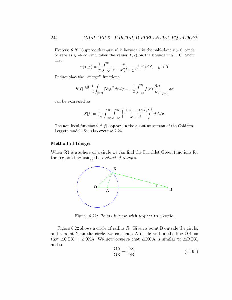
244 CHAPTER 6. PARTIAL DIFFERENTIAL EQUATIONS
Exercise 6.10: Suppose that ϕ(x, y) is harmonic in the half-plane y > 0, tendsto zero as y → ∞, and takes the values f(x) on the boundary y = 0. Showthat
ϕ(x, y) =1
π
∫ ∞
−∞
y
(x− x′)2 + y2f(x′) dx′, y > 0.
Deduce that the “energy” functional
S[f ]def=
1
2
∫
y>0|∇ϕ|2 dxdy ≡ −1
2
∫ ∞
−∞f(x)
∂ϕ
∂y
∣∣∣∣y=0
dx
can be expressed as
S[f ] =1
4π
∫ ∞
−∞
∫ ∞
−∞
f(x)− f(x′)
x− x′2
dx′dx.
The non-local functional S[f ] appears in the quantum version of the Caldeira-Leggett model. See also exercise 2.24.
Method of Images
When ∂Ω is a sphere or a circle we can find the Dirichlet Green functions forthe region Ω by using the method of images .
A BO
X
Figure 6.22: Points inverse with respect to a circle.
Figure 6.22 shows a circle of radius R. Given a point B outside the circle,and a point X on the circle, we construct A inside and on the line OB, sothat ∠OBX = ∠OXA. We now observe that XOA is similar to BOX,and so
OA
OX=
OX
OB. (6.195)
6.5. POTENTIAL THEORY 245
Thus, OA × OB = (OX)2 ≡ R2. The points A and B are therefore mutuallyinverse with respect to the circle. In particular, the point A does not dependon which point X was chosen.
Now let AX= ri, BX= r0 and OB= B. Then, using similar trianglesagain, we have
AX
OX=
BX
OB, (6.196)
orR
ri=B
r0, (6.197)
and so1
ri
(R
B
)− 1
r0= 0. (6.198)
Interpreting the figure as a slice through the centre of a sphere of radius R,we see that if we put a unit charge at B, then the insertion of an image chargeof magnitude q = −R/B at A serves to the keep the entire surface of thesphere at zero potential.
Thus, in three dimensions, and with Ω the region exterior to the sphere,the Dirichlet Green function is
gΩ(r, rB) =1
4π
(1
|r− rB|−(R
|rB|
)1
|r− rA|
). (6.199)
In two dimensions, we find similarly that
gΩ(r, rB) = −1
2π
(ln |r− rB| − ln |r− rA| − ln (|rB|/R)
), (6.200)
has gΩ(r, rB) = 0 for r on the circle. Thus, this is the Dirichlet Green functionfor Ω, the region exterior to the circle.
We can use the same method to construct the interior Green functionsfor the sphere and circle.
6.5.6 Kirchhoff vs. Huygens
Even if we do not have a Green function tailored for the specific region inwhich were are interested, we can still use the whole-space Green functionto convert the differential equation into an integral equation, and so makeprogress. An example of this technique is provided by Kirchhoff’s partialjustification of Huygens’ construction.

246 CHAPTER 6. PARTIAL DIFFERENTIAL EQUATIONS
The Green function G(r, r′) for the elliptic Helmholtz equation
(−∇2 + κ2)G(r, r′) = δ3(r− r′) (6.201)
in R3 is given by
∫d3k
(2π)3eik·(r−r′)
k2 + κ2=
1
4π|r− r′|e−κ|r−r′|. (6.202)
Exercise 6.11: Perform the k integration and confirm this.
For solutions of the wave equation with e−iωt time dependence, we wanta Green function such that
[−∇2 −
(ω2
c2
)]G(r, r′) = δ3(r− r′), (6.203)
and so we have to take κ2 negative. We therefore have two possible Greenfunctions
G±(r, r′) =
1
4π|r− r′|e±ik|r−r′|, (6.204)
where k = |ω|/c. These correspond to taking the real part of κ2 negative, butgiving it an infinitesimal imaginary part, as we did when discussing resolventoperators in chapter 5. If we want outgoing waves, we must take G ≡ G+.
Now suppose we want to solve
(∇2 + k2)ψ = 0 (6.205)
in an arbitrary region Ω. As before, we use Green’s theorem to write
∫
Ω
G(r, r′)(∇2
r + k2)ψ(r)− ψ(r)(∇2r + k2)G(r, r′)
dnx
=
∫
∂Ω
G(r, r′)∇rψ(r)− ψ(r)∇rG(r, r′) · dSr (6.206)
where dSr = n dSr, with n the outward normal to ∂Ω at the point r. Theleft hand side is
∫
Ω
ψ(r)δn(r− r′) dnx =
ψ(r′), r′ ∈ Ω0, r′ /∈ Ω
(6.207)

6.5. POTENTIAL THEORY 247
and so
ψ(r′) =
∫
∂Ω
G(r, r′)(n · ∇x)ψ(r)− ψ(r)(n · ∇r)G(r, r′) dSr, r′ ∈ Ω.
(6.208)This must not be thought of as solution to the wave equation in terms of anintegral over the boundary, analogous to the solution (6.193) of the Dirichletproblem that we found in the last section. Here, unlike that earlier case,G(r, r′) knows nothing of the boundary ∂Ω, and so both terms in the surfaceintegral contribute to ψ. We therefore have a formula for ψ(r) in the interiorin terms of both Dirichlet and Neumann data on the boundary ∂Ω, andgiving both over-prescribes the problem. If we take arbitrary values for ψand (n · ∇)ψ on the boundary, and plug them into (6.208) so as to computeψ(r) within Ω then there is no reason for the resulting ψ(r) to reproduce, as rapproaches the boundary, the values ψ and (n·∇)ψ appearing in the integral.If we demand that the output ψ(r) does reproduce the input boundary data,then this is equivalent to demanding that the boundary data come from asolution of the differential equation in a region encompassing Ω.
B
A
θR
n r
r’
Ω
Figure 6.23: Huygens’ construction.
The mathematical inconsistency of assuming arbitrary boundary datanotwithstanding, this is exactly what we do when we follow Kirchhoff anduse (6.208) to provide a justification of Huygens’ construction as used in

248 CHAPTER 6. PARTIAL DIFFERENTIAL EQUATIONS
optics. Consider the problem of a plane wave, ψ = eikx, incident on a screenfrom the left and passing though the aperture labelled AB in figure 6.23.
We take as the region Ω everything to the right of the obstacle. The Kirch-hoff approximation consists of assuming that the values of ψ and (n · ∇)ψon the surface AB are eikx and −ikeikx, the same as they would be if theobstacle were not there, and that they are identically zero on all other partsof the boundary. In other words, we completely ignore any scattering bythe material in which the aperture resides. We can then use our formula toestimate ψ in the region to the right of the aperture. If we further set
∇rG(r, r′) ≈ ik
(r− r′)
|r− r′|2 eik|r−r′|, (6.209)
which is a good approximation provided we are more than a few wavelengthsaway from the aperture, we find
ψ(r′) ≈ k
4πi
∫
aperture
eik|r−r′|
|r− r′| (1 + cos θ)dSr. (6.210)
Thus, each part of the wavefront on the surface AB acts as a source for thediffracted wave in Ω.
This result, although still an approximation, provides two substantialimprovements to the naıve form of Huygens’ construction as presented inelementary courses:
i) There is factor of (1 + cos θ) which suppresses backward propagatingwaves. The traditional exposition of Huygens construction takes nonotice of which way the wave is going, and so provides no explanationas to why a wavefront does not act a source for a backward wave.
ii) There is a factor of i−1 = e−iπ/2 which corrects a 90 error in the phasemade by the naıve Huygens construction. For two-dimensional slitgeometry we must use the more complicated two-dimensional Greenfunction (it is a Bessel function), and this provides an e−iπ/4 factorwhich corrects for the 45 phase error that is manifest in the Cornuspiral of Fresnel diffraction.
For this reason the Kirchhoff approximation is widely used.
Problem 6.12: Use the method of images to construct i) the Dirichlet, andii) the Neumann, Green function for the region Ω, consisting of everything tothe right of the screen. Use your Green functions to write the solution to the

6.6. FURTHER EXERCISES AND PROBLEMS 249
diffraction problem in this region a) in terms of the values of ψ on the aperturesurface AB, b) in terms of the values of (n · ∇)ψ on the aperture surface. Ineach case, assume that the boundary data are identically zero on the dark sideof the screen. Your expressions should coincide with the Rayleigh-Sommerfelddiffraction integrals of the first and second kind, respectively.3 Explore thedifferences between the predictions of these two formulæ and that of Kirchhofffor case of the diffraction of a plane wave incident on the aperture from theleft.
6.6 Further Exercises and problems
Problem 6.13: Critical Mass. An infinite slab of fissile material has thicknessL. The neutron density n(x) in the material obeys the equation
∂n
∂t= D
∂2n
∂x2+ λn+ µ,
where n(x, t) is zero at the surface of the slab at x = 0, L. Here, D is theneutron diffusion constant, the term λn describes the creation of new neutronsby induced fission, and the constant µ is the rate of production per unit volumeof neutrons by spontaneous fission.
a) Expand n(x, t) as a series,
n(x, t) =∑
m
am(t)ϕm(x),
where the ϕm(x) are a complete set of functions you think suitable forsolving the problem.
b) Find an explicit expression for the coefficients am(t) in terms of theirintial values am(0).
c) Determine the critical thickness Lcrit above which the slab will explode.d) Assuming that L < Lcrit, find the equilibrium distribution neq(x) of
neutrons in the slab. (You may either sum your series expansion to get anexplicit closed-form answer, or use another (Green function?) method.)
Problem 6.14: Semi-infinite Rod. Consider the heat equation
∂θ
∂t= D∇2θ, 0 < x <∞,
with the temperature θ(x, t) obeying the initial condition θ(x, 0) = θ0 for0 < x <∞, and the boundary condition θ(0, t) = 0.
3M. Born and E. Wolf Principles of Optics 7th (expanded) edition, section 8.11.

250 CHAPTER 6. PARTIAL DIFFERENTIAL EQUATIONS
a) Show that the boundary condition at x = 0 may be satisfied at all timesby introducing a suitable mirror image of the initial data in the region−∞ < x < 0, and then applying the heat kernel for the entire realline to this extended initial data. Show that the resulting solution of thesemi-infinite rod problem can be expressed in terms of the error function
erf (x)def=
2√π
∫ x
0e−ξ
2
dξ,
as
θ(x, t) = θ0 erf
(x√4t
).
b) Solve the same problem by using a Fourier integral expansion in termsof sin kx on the half-line 0 < x < ∞ and obtaining the time evolutionof the Fourier coefficients. Invert the transform and show that youranswer reduces to that of part a). (Hint: replace the initial condition byθ(x, 0) = θ0e
−ǫx, so that the Fourier transform converges, and then takethe limit ǫ→ 0 at the end of your calculation.)
Exercise 6.15: Seasonal Heat Waves. Suppose that the measured temperatureof the air above the arctic permafrost at time t is expressed as a Fourier series
θ(t) = θ0 +
∞∑
n=1
θn cosnωt,
where the period T = 2π/ω is one year. Solve the heat equation for the soiltemperature,
∂θ
∂t= κ
∂2θ
∂z2, 0 < z <∞
with this boundary condition, and find the temperature θ(z, t) at a depth zbelow the surface as a function of time. Observe that the sub-surface temper-ature fluctuates with the same period as that of the air, but with a phase lagthat depends on the depth. Also observe that the longest-period temperaturefluctuations penetrate the deepest into the ground. (Hint: for each Fouriercomponent, write θ as Re[An(z) exp inωt], where An is a complex function ofz.)
The next problem is an illustration of a Dirichlet principle.
Exercise 6.16: Helmholtz-Hodge decomposition. Given a three-dimensionalregion Ω with smooth boundary ∂Ω, introduce the real Hilbert space L2
vec(Ω)of finite-norm vector fields, with inner product
〈u,v〉 =∫
Ωu · v d3x.
6.6. FURTHER EXERCISES AND PROBLEMS 251
Consider the spaces L = v : v = ∇φ and T = v : v = curlw consistingof vector fields in L2
vec(Ω) that can can be written as gradients and curls,respectively. (Strictly speaking, we should consider the completions of thesespaces.)
a) Show that if we demand that either (or both) of φ and the tangentialcomponent of w vanish on ∂Ω, then the two spaces L and T are mutuallyorthogonal with respect to the the L2
vec(Ω) inner product.
Let u ∈ L2vec(Ω). We will try to express u as the sum of a gradient and a curl
by seeking to make the distance functional
Fu[φ,w] = ‖u−∇φ− curlw‖2def=
∫
Ω|u−∇φ− curlw|2 d3x
equal to zero.
b) Show that if we find a w and φ that minimize Fu[φ,w], then the residualvector field
hdef= u−∇φ− curlw
obeys curlh = 0 and divh = 0, together with boundary conditionsdetermined by the constraints imposed on φ and w:i) If φ is unconstrained on ∂Ω, but the tangential boundary component
of w is required to vanish, then the component of h normal to theboundary must be zero.
ii) If φ = 0 on ∂Ω, but the tangential boundary component of w isunconstrained, then the tangential boundary component of h mustbe zero.
iii) If φ = 0 on ∂Ω and also the tangential boundary component of w isrequired to vanish, then h need satisfy no boundary condition.
c) Assuming that we can find suitable minimizing φ and w, deduce thatunder each of the three boundary conditions of the previous part, wehave a Helmholtz-Hodge decomposition
u = ∇φ+ curlw + h
into unique parts that are mutually L2vec(Ω) orthogonal. Observe that
the residual vector field h is harmonic — i.e. it satisfies the equation∇2h = 0, where
∇2hdef= ∇(divh)− curl (curlh)
is the vector Laplacian acting on h.

252 CHAPTER 6. PARTIAL DIFFERENTIAL EQUATIONS
If u is sufficiently smooth, there will exist φ and w that minimize the distance‖u−∇φ− curlw‖ and satisfy the boundary conditions. Whether or not h isneeded in the decomposition is another matter. It depends both on how weconstrain φ and w, and on the topology of Ω. At issue is whether or not theboundary conditions imposed on h are sufficient to force it to be zero. If Ωis the interior of a torus, for example, then h can be non-zero whenever itstangential component is unconstrained.
The Helmholtz-Hodge decomposition is closely related to the vector-fieldeigenvalue problems commonly met with in electromagnetism or elasticity.The next few exercises lead up to this connection.
Exercise 6.17: Self-adjointness and the vector Laplacian. Consider the vectorLaplacian (defined in the previous problem) as a linear operator on the Hilbertspace L2
vec(Ω) .
a) Show that∫
Ωd3x
u · (∇2v) − v · (∇2u)
=
∫
∂Ω(n · u) div v− (n · v) div u
−u · (n× curlv) + v · (n× curlu) dS
b) Deduce from the identity in part a) that the domain of ∇2 coincideswith the domain of (∇2)†, and hence the vector Laplacian defines a trulyself-adjoint operator with a complete set of mutually orthogonal eigen-functions, when we take as boundary conditions one of the following:o) Dirichlet-Dirichlet: n · u = 0 and n× u = 0 on ∂Ω,i) Dirichlet-Neumann: n · u = 0 and n× curlu = 0 on ∂Ω,ii) Neumann-Dirichlet: divu = 0 and n× u = 0 on ∂Ω,iii) Neumann-Neumann: divu = 0 and n× curlu = 0 on ∂Ω.
c) Show that the more general Robin boundary conditions
α(n · u) + β divu = 0,
λ(n× u) + µ(n× curlu) = 0,
where α β, µ ν can be position dependent, also give rise to a truly self-adjoint operator.
Problem 6.18: Cavity electrodynamics and the Hodge-Weyl decomposition.Each of the self-adjoint boundary conditions in the previous problem givesrise to a complete set of mutually orthogonal vector eigenfunctions obeying
−∇2un = k2nun.

6.6. FURTHER EXERCISES AND PROBLEMS 253
For these eigenfunctions to describe the normal modes of the electric field E
and the magnetic field B (which we identify with H as we will use units inwhich µ0 = ǫ0 = 1) within a cavity bounded by a perfect conductor, we needto additionally impose the Maxwell equations divB = divE = 0 everywherewithin Ω, and to satisfy the perfect-conductor boundary conditions n × E =n ·B = 0.
a) For each eigenfunction un corresponding to a non-zero eigenvalue k2n,define
vn =1
k2ncurl (curlun), wn = − 1
k2n∇(divun),
so that un = vn + wn. Show that vn and wm are, if non-zero, eacheigenfunctions of −∇2 with eigenvalue k2n. The vector eigenfunctionsthat are not in the null-space of ∇2 can therefore be decomposed intotheir transverse (the vn, which obey divvn = 0) and longitudinal (thewn, which obey curlwn = 0) parts. However, it is not immediately clearwhat boundary conditions the vn and wn separately obey.
b) The boundary-value problems of relevance to electromagnetism are:
i)
−∇2hn = k2nhn, within Ω,n · hn = 0, n× curlhn = 0, on ∂Ω;
ii)
−∇2en = k2nen, within Ω,div en = 0, n× en = 0, on ∂Ω;
iii)
−∇2bn = k2nbn, within Ω,divbn = 0, n× curlbn = 0, on ∂Ω,
These problems involve, respectively, the Dirichlet-Neumann, Neumann-Dirichlet, and Neumann-Neumann boundary conditions from the previ-ous problem.Show that the divergence-free transverse eigenfunctions
Hndef=
1
k2ncurl (curlhn), En
def=
1
k2ncurl (curl en), Bn
def=
1
k2ncurl (curlbn),
obey n ·Hn = n×En = n× curlBn = 0 on the boundary, and that fromthese and the eigenvalue equations we can deduce that n × curlHn =n·Bn = n·curlEn = 0 on the boundary. The perfect-conductor boundaryconditions are therefore satisfied.Also show that the corresponding longitudinal eigenfunctions
ηndef=
1
k2n∇(divhn), ǫn
def=
1
k2n∇(div en), βn
def=
1
k2n∇(divbn)
obey the boundary conditions n · ηn = n× ǫn = n× βn = 0.

254 CHAPTER 6. PARTIAL DIFFERENTIAL EQUATIONS
c) By considering the counter-example provided by a rectangular box, showthat the Dirichlet-Dirichlet boundary condition is not compatible with alongitudinal+transverse decomposition. (A purely transverse wave inci-dent on such a boundary will, on reflection, acquire a longitudinal com-ponent.)
d) Show that
0 =
∫
Ωηn ·Hm d
3x =
∫
Ωǫn · Em d
3x =
∫
Ωβn ·Bm d
3x,
but that the vn and wn obtained from the Dirichlet-Dirichlet boundarycondition un’s are not in general orthogonal to each other. Use thecontinuity of the L2
vec(Ω) inner product
xn → x ⇒ 〈xn,y〉 → 〈x,y〉
to show that this individual-eigenfunction orthogonality is retained bylimits of sums of the eigenfunctions. Deduce that, for each of the bound-ary conditions i)-iii) (but not for the Dirichlet-Dirichlet case), we havethe Hodge-Weyl decomposition of L2
vec(Ω) as the orthogonal direct sum
L2vec(Ω) = L ⊕ T ⊕N ,
where L, T are respectively the spaces of functions representable as in-finite sums of the longitudinal and transverse eigenfunctions, and N isthe finite-dimensional space of harmonic (nullspace) eigenfunctions.
Complete sets of vector eigenfunctions for the interior of a rectangular box,and for each of the four sets of boundary conditions we have considered, canbe found in Morse and Feshbach §13.1.
Problem 6.19: Hodge-Weyl and Helmholtz-Hodge. In this exercise we considerthe problem of what classes of vector-valued functions can be expanded interms of the various families of eigenfunctions of the previous problem. It istempting (but wrong) to think that we are restricted to expanding functionsthat obey the same boundary conditions as the eigenfunctions themselves.Thus, we might erroniously expect that the En are good only for expandingfunctions whose divergence vanishes and have vanishing tangential boundarycomponents, or that the ηn can expand out only curl-free vector fields withvanishing normal boundary component. That this supposition can be falsewas exposed in section 2.2.3, where we showed that functions that are zero atthe endpoints of an interval can be used to expand out functions that are notzero there. The key point is that each of our four families of un constitute
6.6. FURTHER EXERCISES AND PROBLEMS 255
a complete orthonormal set in L2vec(Ω), and can therefore be used expand
any vector field. As a consequence, the infinite sum∑anEn ∈ T can, for
example, represent any vector-valued function u ∈ L2vec(Ω) provided only that
u possesses no component lying either in the subspace L of the longitudinaleigenfunctions ǫn, or in the nullspace N .
a) Let T =< En > be space of functions representable as infinite sums ofthe En. Show that
< En >⊥= u : curlu = 0 within Ω, n× u = 0 on ∂Ω.
Similarly show that
< ǫn >⊥ = u : divu = 0 within Ω, no condition on ∂Ω,
< Hn >⊥ = u : curlu = 0 within Ω, no condition on ∂Ω,
< ηn >⊥ = u : divu = 0 within Ω, n · u = 0 on ∂Ω,
< Bn >⊥ = u : curlu = 0 within Ω, no condition on ∂Ω.
< βn >⊥ = u : divu = 0 within Ω, no condition on ∂Ω,
b) Use the results of part (a) and the Helmholtz-Hodge decomposition toshow that
< En > = u ∈ L2vec(Ω) : u = curlw, no condition on w on ∂Ω.
< ǫn > = u ∈ L2vec(Ω) : u = ∇φ, where φ = 0 on ∂Ω,
< Hn > = u ∈ L2vec(Ω) : u = curlw, where n×w = 0 on ∂Ω,
< ηn > = u ∈ L2vec(Ω) : u = ∇φ, no condition on φ on ∂Ω,
< Bn > = u ∈ L2vec(Ω) : u = curlw, where n×w = 0 on ∂Ω.
< βn > = u ∈ L2vec(Ω) : u = ∇φ, where φ = 0 on ∂Ω.
c) Conclude from the previous part, that the Hodge-Weyl eigenspace de-compositions
L2vec(Ω) = L ⊕ T ⊕N
for each of the three vector Laplacian boundary condition families (i),(ii) and (iii) coincides the Helmholtz-Hodge decompositions under theconditions (i), (ii) and (iii) in problem 6.16
d) As an illustration of the practical distinctions between the decomposi-tions in part (c), take Ω to be the unit cube in R3, and u = (1, 0, 0) aconstant vector field. Show that with conditions (i) we have u ∈ L, butfor (ii) we have u ∈ T , and for (iii) we have u ∈ N .

256 CHAPTER 6. PARTIAL DIFFERENTIAL EQUATIONS

Chapter 7
The Mathematics of RealWaves
Waves are found everywhere in the physical world, but we often need morethan the simple wave equation to understand them. The principal compli-cations are non-linearity and dispersion. In this chapter we will describe themathematics lying behind some commonly observed, but still fascinating,phenomena.
7.1 Dispersive waves
In this section we will investigate the effects of dispersion, the dependenceof the speed of propagation on the frequency of the wave. We will see thatdispersion has a profound effect on the behaviour of a wave-packet.
7.1.1 Ocean Waves
The most commonly seen dispersive waves are those on the surface of water.Although often used to illustrate wave motion in class demonstrations, thesewaves are not as simple as they seem.
In chapter one we derived the equations governing the motion of waterwith a free surface. Now we will solve these equations. Recall that wedescribed the flow by introducing a velocity potential φ such that, v = ∇φ,and a variable h(x, t) which is the depth of the water at abscissa x.
257

258 CHAPTER 7. THE MATHEMATICS OF REAL WAVES
y
x
0
0P
h(x,t)
ρ
g
Figure 7.1: Water with a free surface.
Again looking back to chapter one, we see that the fluid motion is determinedby imposing
∇2φ = 0 (7.1)
everywhere in the bulk of the fluid, together with boundary conditions
∂φ
∂y= 0, on y = 0, (7.2)
∂φ
∂t+
1
2(∇φ)2 + gy = 0, on the free surface y = h, (7.3)
∂h
∂t− ∂φ
∂y+∂h
∂x
∂φ
∂x= 0, on the free surface y = h. (7.4)
Recall the physical interpretation of these equations: The vanishing of theLaplacian of the velocity potential simply means that the bulk flow is incom-pressible
divv = ∇2φ = 0. (7.5)
The first two of the boundary conditions are also easy to interpret: The firstsays that no water escapes through the lower boundary at y = 0. The second,a form of Bernoulli’s equation, asserts that the free surface is everywhere atconstant (atmospheric) pressure. The remaining boundary condition is moreobscure. It states that a fluid particle initially on the surface stays on thesurface. Remember that we set f(x, y, t) = h(x, t) − y, so the water surfaceis given by f(x, y, t) = 0. If the surface particles are carried with the flowthen the convective derivative of f ,
df
dtdef=∂f
∂t+ (v · ∇)f, (7.6)

7.1. DISPERSIVE WAVES 259
should vanish on the free surface. Using v = ∇φ and the definition of f , thisreduces to
∂h
∂t+∂φ
∂x
∂h
∂x− ∂φ
∂y= 0, (7.7)
which is indeed the last boundary condition.Using our knowledge of solutions of Laplace’s equation, we can immedi-
ately write down a wave-like solution satisfying the boundary condition aty = 0
φ(x, y, t) = a cosh(ky) cos(kx− ωt). (7.8)
The tricky part is satisfying the remaining two boundary conditions. Thedifficulty is that they are non-linear, and so couple modes with differentwave-numbers. We will circumvent the difficulty by restricting ourselves tosmall amplitude waves, for which the boundary conditions can be linearized.Suppressing all terms that contain a product of two or more small quantities,we are left with
∂φ
∂t+ gh = 0, (7.9)
∂h
∂t− ∂φ
∂y= 0. (7.10)
Because φ is a already a small quantity, and the wave amplitude is a smallquantity, linearization requires that these equations should be imposed atthe equilibrium surface of the fluid y = h0. It is convenient to eliminate h toget
∂2φ
∂t2+ g
∂φ
∂y= 0, on y = h0. (7.11)
Inserting (7.8) into this boundary condition leads to the dispersion equation
ω2 = gk tanh kh0, (7.12)
relating the frequency to the wave-number.Two limiting cases are of particular interest:
i) Long waves on shallow water: Here kh0 ≪ 1, and, in this limit,
ω = k√gh0.
ii) Waves on deep water: Here, kh0 ≫ 1, leading to ω =√gk.

260 CHAPTER 7. THE MATHEMATICS OF REAL WAVES
For deep water, the velocity potential becomes
φ(x, y, t) = aek(y−h0) cos(kx− ωt). (7.13)
We see that the disturbance due to the surface wave dies away exponentially,and becomes very small only a few wavelengths below the surface.
Remember that the velocity of the fluid is v = ∇φ. To follow the motionof individual particles of fluid we must solve the equations
dx
dt= vx = −akek(y−h0) sin(kx− ωt),
dy
dt= vy = akek(y−h0) cos(kx− ωt). (7.14)
This is a system of coupled non-linear differential equations, but to findthe small amplitude motion of particles at the surface we may, to a firstapproximation, set x = x0, y = h0 on the right-hand side. The orbits of thesurface particles are therefore approximately
x(t) = x0 −ak
ωcos(kx0 − ωt),
y(t) = y0 −ak
ωsin(kx0 − ωt). (7.15)
x
y
Figure 7.2: Circular orbits in deep water surface waves.
For right-moving waves, the particle orbits are clockwise circles. At thewave-crest the particles move in the direction of the wave propagation; inthe troughs they move in the opposite direction. Figure 7.2 shows that thismotion results in an up-down-asymmetric cycloidal wave profile.
When the effect of the bottom becomes significant, the circular orbitsdeform into ellipses. For shallow water waves, the motion is principally back-and-forth with motion in the y direction almost negligeable.

7.1. DISPERSIVE WAVES 261
7.1.2 Group Velocity
The most important effect of dispersion is that the group velocity of the waves— the speed at which a wave-packet travels — differs from the phase velocity— the speed at which individual wave-crests move. The group velocity isalso the speed at which the energy associated with the waves travels.
Suppose that we have waves with dispersion equation ω = ω(k). A right-going wave-packet of finite extent, and with initial profile ϕ(x), can be Fourieranalyzed to give
ϕ(x) =
∫ ∞
−∞
dk
2πA(k)eikx. (7.16)
x
Figure 7.3: A right-going wavepacket.
At later times this will evolve to
ϕ(x, t) =
∫ ∞
−∞
dk
2πA(k)eikx−iω(k)t. (7.17)
Let us suppose for the moment that A(k) is non-zero only for a narrow bandof wavenumbers around k0, and that, restricted to this narrow band, we canapproximate the full ω(k) dispersion equation by
ω(k) ≈ ω0 + U(k − k0). (7.18)
Thus
ϕ(x, t) =
∫ ∞
−∞
dk
2πA(k)eik(x−Ut)−i(ω0−Uk0)t. (7.19)
Comparing this with the Fourier expression for the initial profile, we findthat
ϕ(x, t) = e−i(ω0−Uk0)tϕ(x− Ut). (7.20)

262 CHAPTER 7. THE MATHEMATICS OF REAL WAVES
The pulse envelope therefore travels at speed U . This velocity
U ≡ ∂ω
∂k(7.21)
is the group velocity . The individual wave crests, on the other hand, moveat the phase velocity ω(k)/k.
When the initial pulse contains a broad range of frequencies we can stillexplore its evolution. We make use of a powerful tool for estimating the be-havior of integrals that contain a large parameter. In this case the parameteris the time t. We begin by writing the Fourier representation of the wave as
ϕ(x, t) =
∫ ∞
−∞
dk
2πA(k)eitψ(k) (7.22)
whereψ(k) = k
(xt
)− ω(k). (7.23)
Now look at the behaviour of this integral as t becomes large, but while wekeep the ratio x/t fixed. Since t is very large, any variation of ψ with kwill make the integrand a very rapidly oscillating function of k. Cancellationbetween adjacent intervals with opposite phase will cause the net contributionfrom such a region of the k integration to be very small. The principalcontribution will come from the neighbourhood of stationary phase points,i.e. points where
0 =dψ
dk=x
t− ∂ω
∂k. (7.24)
This means that, at points in space where x/t = U , we will only get contri-butions from the Fourier components with wave-number satisfying
U =∂ω
∂k. (7.25)
The initial packet will therefore spread out, with those components of thewave having wave-number k travelling at speed
vgroup =∂ω
∂k. (7.26)
This is the same expression for the group velocity that we obtained in thenarrow-band case. Again this speed of propagation should be contrastedwith that of the wave-crests, which travel at
vphase =ω
k. (7.27)

7.1. DISPERSIVE WAVES 263
The “stationary phase” argument may seem a little hand-waving, but it canbe developed into a systematic approximation scheme. We will do this inchapter 19.
Example: Water Waves. The dispersion equation for waves on deep water isω =√gk. The phase velocity is therefore
vphase =
√g
k, (7.28)
whilst the group velocity is
vgroup =1
2
√g
k=
1
2vphase. (7.29)
This difference is easily demonstrated by tossing a stone into a pool andobserving how individual wave-crests overtake the circular wave packet anddie out at the leading edge, while new crests and troughs come into being atthe rear and make their way to the front.
This result can be extended to three dimensions with
vigroup =∂ω
∂ki(7.30)
Example: de Broglie Waves. The plane-wave solutions of the time-dependentSchrodinger equation
i∂ψ
∂t= − 1
2m∇2ψ, (7.31)
are
ψ = eik·r−iωt, (7.32)
with
ω(k) =1
2mk2. (7.33)
The group velocity is therefore
vgroup =1
mk, (7.34)
which is the classical velocity of the particle.

264 CHAPTER 7. THE MATHEMATICS OF REAL WAVES
7.1.3 Wakes
There are many circumstances when waves are excited by object moving ata constant velocity through a background medium, or by a stationary objectimmersed in a steady flow. The resulting wakes carry off energy, and thereforecreate wave drag . Wakes are involved, for example, in sonic booms, Cerenkovradiation, the Landau criterion for superfluidity, and Landau damping ofplasma oscillations. Here, we will consider some simple water-wave analoguesof these effects. The common principle for all wakes is that the resulting wavepattern is time independent when observed from the object exciting it.Example: Obstacle in a Stream. Consider a log lying submerged in a rapidlyflowing stream.
v v
Figure 7.4: Log in a stream.
The obstacle disturbs the water and generates a train of waves. If the log liesathwart the stream, the problem is essentially one-dimensional and easy toanalyse. The essential point is that the distance of the wavecrests from the logdoes not change with time, and therefore the wavelength of the disturbancethe log creates is selected by the condition that the phase velocity of the wave,coincide with the velocity of the mean flow.1 The group velocity does comeinto play, however. If the group velocity of the waves is less that the phasevelocity, the energy being deposited in the wave-train by the disturbance willbe swept downstream, and the wake will lie behind the obstacle. If the groupvelocity is higher than the phase velocity, and this is the case with very shortwavelength ripples on water where surface tension is more important thangravity, the energy will propagate against the flow, and so the ripples appearupstream of the obstacle.
1In his book Waves in Fluids , M. J. Lighthill quotes Robert Frost on this phenomenon:
The black stream, catching on a sunken rock,Flung backward on itself in one white wave,And the white water rode the black forever,Not gaining but not losing.

7.1. DISPERSIVE WAVES 265
A B
C
D
θO
Figure 7.5: Kelvin’s ship-wave construction.
Example: Kelvin Ship Waves. A more subtle problem is the pattern of wavesleft behind by a ship on deep water. The shape of the pattern is determinedby the group velocity for deep-water waves being one-half that of the phasevelocity.
How the wave pattern is formed can be understood from figure 7.5. Inorder that the pattern of wavecrests be time independent, the waves emittedin the direction AC must have phase velocity such that their crests travelfrom A to C while the ship goes from A to B. The crest of the wave emittedfrom the bow of the ship in the direction AC will therefore lie along the lineBC — or at least there would be a wave crest on this line if the emittedwave energy travelled at the phase velocity. The angle at C must be a rightangle because the direction of propagation is perpendicular to the wave-crests. Euclid, by virtue of his angle-in-a-semicircle theorem, now tells usthat the locus of all possible points C (for all directions of wave emission)is the larger circle. Because, however, the wave energy only travels at one-half the phase velocity, the waves going in the direction AC actually havesignificant amplitude only on the smaller circle, which has half the radius ofthe larger. The wake therefore lies on, and within, the Kelvin wedge, whoseboundary lies at an angle θ to the ship’s path. This angle is determined bythe ratio OD/OB=1/3 to be
θ = sin−1(1/3) = 19.5. (7.35)
Remarkably, this angle, and hence the width of the wake, is independent ofthe speed of the ship.
The waves actually on the edge of the wedge are usually the most promi-

266 CHAPTER 7. THE MATHEMATICS OF REAL WAVES
Figure 7.6: Large-scale Kelvin wakes. (Image source: US Navy)
nent, and they will have crests perpendicular to the line AD. This orientationis indicated on the left hand figure, and reproduced as the predicted patternof wavecrests on the right. The prediction should be compared with the wavesystems in figures 7.6 and 7.7.
7.1.4 Hamilton’s Theory of Rays
We have seen that wave packets travel at a frequency-dependent group ve-locity. We can extend this result to study the motion of waves in weaklyinhomogeneous media, and so derive an analogy between the “geometric op-tics” limit of wave motion and classical dynamics.
Consider a packet composed of a roughly uniform train of waves spreadout over a region that is substantially longer and wider than their mean wave-length. The essential feature of such a wave train is that at any particularpoint of space and time, x and t, it has a definite phase Θ(x, t). Once weknow this phase, we can define the local frequency ω and wave-vector k by
ω = −(∂Θ
∂t
)
x
, ki =
(∂Θ
∂xi
)
t
. (7.36)

7.1. DISPERSIVE WAVES 267
Figure 7.7: Small-scale Kelvin wake. (Phograph by Fabrice Neyret)
These definitions are motivated by the idea that
Θ(x, t) ∼ k · x− ωt, (7.37)
at least locally.
We wish to understand how k changes as the wave propagates through aslowly varying medium. We introduce the inhomogeneity by assuming thatthe dispersion equation ω = ω(k), which is initially derived for a uniformmedium, can be extended to ω = ω(k,x), where the x dependence arises,for example, as a result of a position-dependent refractive index. This as-sumption is only an approximation, but it is a good approximation when thedistance over which the medium changes is much larger than the distancebetween wavecrests.
Applying the equality of mixed partials to the definitions of k and ω givesus (
∂ω
∂xi
)
t
= −(∂ki∂t
)
x
,
(∂ki∂xj
)
xi
=
(∂kj∂xi
)
xj
. (7.38)
The subscripts indicate what is being left fixed when we differentiate. Wemust be careful about this, because we want to use the dispersion equation

268 CHAPTER 7. THE MATHEMATICS OF REAL WAVES
to express ω as a function of k and x, and the wave-vector k will itself be afunction of x and t.
Taking this dependence into account, we write(∂ω
∂xi
)
t
=
(∂ω
∂xi
)
k
+
(∂ω
∂kj
)
x
(∂kj∂xi
)
t
. (7.39)
We now use (7.38) to rewrite this as(∂ki∂t
)
x
+
(∂ω
∂kj
)
x
(∂ki∂xj
)
t
= −(∂ω
∂xi
)
k
. (7.40)
Interpreting the left hand side as a convective derivative
dkidt
=
(∂ki∂t
)
x
+ (vg · ∇)ki,
we read off thatdkidt
= −(∂ω
∂xi
)
k
(7.41)
provided we are moving at velocity
dxidt
= (vg)i =
(∂ω
∂ki
)
x
. (7.42)
Since this is the group velocity, the packet of waves is actually travelling atthis speed. The last two equations therefore tell us how the orientation andwavelength of the wave train evolve if we ride along with the packet as it isrefracted by the inhomogeneity.
The formulæ
k = −∂ω∂x
,
x =∂ω
∂k, (7.43)
are Hamilton’s ray equations . These Hamilton equations are identical in formto Hamilton’s equations for classical mechanics
p = −∂H∂x
,
x =∂H
∂p, (7.44)
7.2. MAKING WAVES 269
except that k is playing the role of the canonical momentum, p, and ω(k,x)replaces the Hamiltonian, H(p,x). This formal equivalence of geometricoptics and classical mechanics was mystery in Hamilton’s time. Today weunderstand that classical mechanics is nothing but the geometric optics limitof wave mechanics.
7.2 Making Waves
Many waves occurring in nature are generated by the energy of some steadyflow being stolen away to drive an oscillatory motion. Familiar examplesinclude the music of a flute and the waves raised on the surface of water bythe wind. The latter process is quite subtle and was not understood until thework of J. W. Miles in 1957. Miles showed that in order to excite waves thewind speed has to vary with the height above the water, and that waves ofa given wavelength take energy only from the wind at that height where thewindspeed matches the phase velocity of the wave. The resulting resonantenergy transfer turns out to have analogues in many branches of science. Inthis section we will exhibit this phenomenon in the simpler situation wherethe varying flow is that of the water itself.
7.2.1 Rayleigh’s Equation
Consider water flowing in a shallow channel where friction forces keep thewater in contact the stream-bed from moving. We will show that the resultingshear flow is unstable to the formation of waves on the water surface. Theconsequences of this instability are most often seen in a thin sheet of waterrunning down the face of a dam. The sheet starts off flowing smoothly, but,as the water descends, waves form and break, and the water reaches thebottom in irregular pulses called roll waves .
It is easiest to describe what is happening from the vantage of a referenceframe that rides along with the surface water. In this frame the velocityprofile of the flow will be as shown in figure 7.8.

270 CHAPTER 7. THE MATHEMATICS OF REAL WAVES
y
y
h U(y)
0
x
Figure 7.8: The velocity profile U(y) in a frame at which the surface is atrest.
Since the flow is incompressible but not irrotational, we will describe themotion by using a stream function Ψ, in terms of which the fluid velocity isgiven by
vx = −∂yΨ,vy = ∂xΨ. (7.45)
This parameterization automatically satisfies ∇ · v = 0, while the (z compo-nent of) the vorticity becomes
Ω ≡ ∂xvy − ∂yvx = ∇2Ψ. (7.46)
We will consider a stream function of the form2
Ψ(x, y, t) = ψ0(y) + ψ(y)eikx−iωt, (7.47)
where ψ0 obeys −∂yψ0 = vx = U(y), and describes the horizontal mean flow.The term containing ψ(y) represents a small-amplitude wave disturbancesuperposed on the mean flow. We will investigate whether this disturbancegrows or decreases with time.
Euler’s equation can be written as,
v + v × Ω = −∇(P +
v2
2+ gy
)= 0. (7.48)
Taking the curl of this, and taking into account the two dimensional characterof the problem, we find that
∂tΩ + (v · ∇)Ω = 0. (7.49)
2The physical stream function is, of course, the real part of this expression.

7.2. MAKING WAVES 271
This, a general property of two-dimensional incompressible motion, says thatvorticity is convected with the flow. We now express (7.49) in terms of Ψ,when it becomes
∇2Ψ + (v · ∇)∇2Ψ = 0. (7.50)
Substituting the expression (7.47) into (7.50), and keeping only terms of firstorder in ψ, gives
−iω(d2
dy2− k2
)ψ + iUk
(d2
dy2− k2
)ψ + ikψ∂y(−∂yU) = 0,
or (d2
dy2− k2
)ψ −
(∂2U
∂y2
)1
(U − ω/k)ψ = 0. (7.51)
This is Rayleigh’s equation.3 If only the first term were present, it wouldhave solutions ψ ∝ e±ky, and we would have recovered the results of section7.1.1. The second term is significant, however. It will diverge if there is apoint yc such that U(yc) = ω/k. In other words, if there is a depth at whichthe flow speed coincides with the phase velocity of the wave disturbance, thusallowing a resonant interaction between the wave and flow. An actual infinityin (7.51) will be evaded, though, because ω will gain a small imaginary partω → ωR + iγ. A positive imaginary part means that the wave amplitude isgrowing exponentially with time. A negative imaginary part means that thewave is being damped. With γ included, we then have
1
(U − ω/k) ≈U − ωR/k
(U − ωR/k)2 + γ2+ iπ sgn
(γk
)δ(U(y)− ωR/k
)
=U − ωR/k
(U − ωR/k)2 + γ2+ iπ sgn
(γk
) ∣∣∣∣∂U
∂y
∣∣∣∣−1
yc
δ(y − yc).
(7.52)
To specify the problem fully we need to impose boundary conditions onψ(y). On the lower surface we can set ψ(0) = 0, as this will keep the fluidat rest there. On the upper surface y = h we apply Euler’s equation
v + v × Ω = −∇(P +
v2
2+ gh
)= 0. (7.53)
3Lord Rayleigh, “On the stability or instability of certain fluid motions.” Proc. Lond.Math. Soc. 11 (1879).

272 CHAPTER 7. THE MATHEMATICS OF REAL WAVES
We observe that P is constant, being atmospheric pressure, and the v2/2 canbe neglected as it is of second order in the disturbance. Then, consideringthe x component, we have
−∇xgh = −g∂x∫ t
vydt = −g(k2
iω
)ψ (7.54)
on the free surface. To lowest order we can apply the boundary condition onthe equilibrium free surface y = y0. The boundary condition is therefore
1
ψ
dψ
dy+k
ω
∂U
∂y= g
k2
ω2, y = y0. (7.55)
We usually have ∂U/∂y = 0 near the surface, so this simplifies to
1
ψ
dψ
dy= g
k2
ω2. (7.56)
That this is sensible can be confirmed by considering the case of waves onstill, deep water, where ψ(y) = e|k|y. The boundary condition then reducesto |k| = gk2/ω2, or ω2 = g|k|, which is the correct dispersion equation forsuch waves.
We find the corresponding dispersion equation for waves on shallow flow-ing water by computing
1
ψ
dψ
dy
∣∣∣∣y0
, (7.57)
from Rayleigh’s equation (7.51). Multiplying by ψ∗ and integrating gives
0 =
∫ y0
0
dy
ψ∗(d2
dy2− k2
)ψ + k
(∂2U
∂y2
)1
(ω − Uk) |ψ|2
. (7.58)
An integration by parts then gives[ψ∗dψ
dy
]y0
0
=
∫ y0
0
dy
∣∣∣∣dψ
dy
∣∣∣∣+ k2|ψ|2 +(∂2U
∂y2
)1
(U − ω/k) |ψ|2
. (7.59)
The lower limit makes no contribution, since ψ∗ is zero there. On using (7.52)and taking the imaginary part, we find
Im
(ψ∗dψ
dy
)
y0
= sgn(γk
)π
(∂2U
∂y2
)
yc
∣∣∣∣∂U
∂y
∣∣∣∣−1
yc
|ψ(yc)|, (7.60)

7.2. MAKING WAVES 273
or
Im
(1
ψ
dψ
dy
)
y0
= sgn(γk
)π
(∂2U
∂y2
)
yc
∣∣∣∣∂U
∂y
∣∣∣∣−1
yc
|ψ(yc)|2|ψ(y0)|2
. (7.61)
This equation is most useful if the interaction with the flow does not sub-stantially perturb ψ(y) away from the still-water result ψ(y) = sinh(|k|y),and assuming this is so provides a reasonable first approximation.
If we insert (7.61) into (7.56), where we approximate,
g
(k2
ω2
)≈ g
(k2
ω2R
)− 2ig
(k2
ω3R
)γ,
we find
γ =ω3R
2gk2Im
(1
ψ
dψ
dy
)
y0
= sgn(γk
)πω3R
2gk2
(∂2U
∂y2
)
yc
∣∣∣∣∂U
∂y
∣∣∣∣−1
yc
|ψ(yc)|2|ψ(y0)|2
. (7.62)
We see that either sign of γ is allowed by our analysis. Thus the resonantinteraction between the shear flow and wave appears to lead to either ex-ponential growth or damping of the wave. This is inevitable because ourinviscid fluid contains no mechanism for dissipation, and its motion is neces-sarily time-reversal invariant. Nonetheless, as in our discussion of “frictionwithout friction” in section 5.2.2, only one sign of γ is actually observed.This sign is determined by the initial conditions, but a rigorous explanationof how this works mathematically is not easy, and is the subject of manypapers. These show that the correct sign is given by
γ = −π ω3R
2gk2
(∂2U
∂y2
)
yc
∣∣∣∣∂U
∂y
∣∣∣∣−1
yc
|ψ(yc)|2|ψ(y0)|2
. (7.63)
Since our velocity profile has ∂2U/∂y2 < 0, this means that the waves growin amplitude.
We can also establish the correct sign for γ by a computing the change ofmomentum in the background flow due to the wave.4 The crucial element iswhether, in the neighbourhood of the critical depth, more fluid is overtakingthe wave than lagging behind it. This is exactly what the the quantity∂2U/∂y2 measures.
4G. E. Vekstein, “Landau resonance mechanism for plasma and wind-generated waterwaves,” American Journal of Physics , 66 (1998) 886-92.

274 CHAPTER 7. THE MATHEMATICS OF REAL WAVES
7.3 Non-linear Waves
Non-linear effects become important when some dimensionless measure ofthe amplitude of the disturbance, say ∆P/P for a sound wave, or ∆h/λ fora water wave, is no longer ≪ 1.
7.3.1 Sound in Air
The simplest non-linear wave system is one-dimensional sound propagationin a gas. This problem was studied by Riemann.
The one dimensional motion of a fluid is determined by the mass conser-vation equation
∂tρ+ ∂x(ρv) = 0, (7.64)
and Euler’s equation of motion
ρ(∂tv + v∂xv) = −∂xP. (7.65)
In a fluid with equation of state P = P (ρ), the speed of sound, c, is given by
c2 =dP
dρ. (7.66)
It will in general depend on P , the speed of propagation being usually higherwhen the pressure is higher.
Riemann was able to simplify these equations by defining a new thermo-dynamic variable π(P ) as
π =
∫ P
P0
1
ρcdP, (7.67)
were P0 is the equilibrium pressure of the undisturbed air. The quantity πobeys
dπ
dP=
1
ρc. (7.68)
In terms of π, Euler’s equation divided by ρ becomes
∂tv + v∂xv + c∂xπ = 0, (7.69)
whilst the equation of mass conservation divided by ρ/c becomes
∂tπ + v∂xπ + c∂xv = 0. (7.70)

7.3. NON-LINEAR WAVES 275
BC
C−
A+
t
xA B
P
Figure 7.9: Non-linear characteristic curves.
Adding and subtracting, we get Riemann’s equations
∂t(v + π) + (v + c)∂x(v + π) = 0,
∂t(v − π) + (v − c)∂x(v − π) = 0. (7.71)
These assert that the Riemann invariants v±π are constant along the char-acteristic curves
dx
dt= v ± c. (7.72)
This tell us that signals travel at the speed v±c. In other words, they travel,with respect to the fluid, at the local speed of sound c. Using the Riemannequations, we can propagate initial data v(x, t = 0), π(x, t = 0) into thefuture by using the method of characteristics.In figure 7.9 the value of v+π is constant along the characteristic curve CA
+ ,which is the solution of
dx
dt= v + c (7.73)
passing through A. The value of v − π is constant along CB− , which is the
solution ofdx
dt= v − c (7.74)
passing through B. Thus the values of π and v at the point P can be found ifwe know the initial values of v + π at the point A and v − π at the point B.Having found v and π at P we can invert π(P ) to find the pressure P , andhence c, and so continue the characteristics into the future, as indicated by

276 CHAPTER 7. THE MATHEMATICS OF REAL WAVES
P
x
t
?
Figure 7.10: Simple wave characteristics.
the dotted lines. We need, of course, to know v and c at every point alongthe characteristics CA
+ and CB− in order to construct them, and this requires
us to to treat every point as a “P”. The values of the dynamical quantitiesat P therefore depend on the initial data at all points lying between A andB. This is the domain of dependence of P
A sound wave caused by a localized excess of pressure will eventuallybreak up into two distinct pulses, one going forwards and one going back-wards. Once these pulses are sufficiently separated that they no longer inter-act with one another they are simple waves . Consider a forward-going pulsepropagating into undisturbed air. The backward characteristics are comingfrom the undisturbed region where both π and v are zero. Clearly π − v iszero everywhere on these characteristics, and so π = v. Now π+v = 2v = 2πis constant the forward characteristics, and so π and v are individually con-stant along them. Since π is constant, so is c. With v also being constant,this means that c + v is constant. In other words, for a simple wave, thecharacteristics are straight lines .
This simple-wave simplification contains within it the seeds of its owndestruction. Suppose we have a positive pressure pulse in a fluid whosespeed of sound increases with the pressure. Figure 7.10 shows how, withthis assumption, the straight-line characteristics travel faster in the highpressure region, and eventually catch up with and intersect the slower-movingcharacteristics. When this happens the dynamical variables will becomemultivalued. How do we deal with this?

7.3. NON-LINEAR WAVES 277
7.3.2 Shocks
Let us untangle the multivaluedness by drawing another set of pictures. Sup-pose u obeys the non-linear “half” wave equation
(∂t + u∂x)u = 0. (7.75)
The velocity of propagation of the wave is therefore u itself, so the parts ofthe wave with large u will overtake those with smaller u, and the wave will“break,” as shown in figure 7.11
u u
u u
a) b)
d)c)?
Figure 7.11: A breaking non-linear wave.
Physics does not permit such multivalued solutions, and what usually hap-pens is that the assumptions underlying the model which gave rise to thenonlinear equation will no longer be valid. New terms should be included inthe equation which prevent the solution becoming multivalued, and insteada steep “shock” will form.
ud’)
Figure 7.12: Formation of a shock.

278 CHAPTER 7. THE MATHEMATICS OF REAL WAVES
Examples of an equation with such additional terms are Burgers’ equation
(∂t + u∂x)u = ν∂2xxu, (7.76)
and the Korteweg de-Vries (KdV) equation (4.11), which, by a suitable rescal-ing of x and t, we can write as
(∂t + u∂x)u = δ ∂3xxxu. (7.77)
Burgers’ equation, for example, can be thought of as including the effects ofthermal conductivity, which was not included in the derivation of Riemann’sequations. In both these modified equations, the right hand side is negligeablewhen u is varying slowly, but it completely changes the character of thesolution when the waves steepen and try to break.
Although these extra terms are essential for the stabilization of the shock,once we know that such a discontinuous solution has formed, we can findmany of its properties — for example the propagation velocity — from generalprinciples, without needing their detailed form. All we need is to know whatconservation laws are applicable.
Multiplying (∂t + u∂x)u = 0 by un−1, we deduce that
∂t
1
nun+ ∂x
1
n + 1un+1
= 0, (7.78)
and this implies that
Qn =
∫ ∞
−∞un dx (7.79)
is time independent. There are infinitely many of these conservation laws,one for each n. Suppose that the n-th conservation law continues to hold evenin the presence of the shock, and that the discontinuity is at X(t). Then
d
dt
∫ X(t)
−∞un dx+
∫ ∞
X(t)
un dx
= 0. (7.80)
This is equal to
un−(X)X − un+(X)X +
∫ X(t)
−∞∂tu
n dx+
∫ ∞
X(t)
∂tun dx = 0, (7.81)

7.3. NON-LINEAR WAVES 279
where un−(X) ≡ un(X−ǫ) and un+(X) ≡ un(X+ǫ). Now, using (∂t+u∂x)u = 0in the regions away from the shock, where it is reliable, we can write this as
(un+ − un−)X = − n
n + 1
∫ X(t)
−∞∂xu
n+1 dx− n
n+ 1
∫ ∞
X(t)
∂xun+1 dx
=
(n
n + 1
)(un+1
+ − un+1− ). (7.82)
The velocity at which the shock moves is therefore
X =
(n
n + 1
)(un+1
+ − un+1− )
(un+ − un−). (7.83)
Since the shock can only move at one velocity, only one of the infinitely manyconservation laws can continue to hold in the modified theory!Example: Burgers’ equation. From
(∂t + u∂x)u = ν∂2xxu, (7.84)
we deduce that
∂tu+ ∂x
1
2u2 − ν∂xu
= 0, (7.85)
so that Q1 =∫u dx is conserved, but further investigation shows that no
other conservation law survives. The shock speed is therefore
X =1
2
(u2+ − u2−)(u+ − u−)
=1
2(u+ + u−). (7.86)
Example: KdV equation. From
(∂t + u∂x)u = δ ∂3xxxu, (7.87)
we deduce that
∂tu+ ∂x
1
2u2 − δ ∂2xxu
= 0,
∂t
1
2u2+ ∂x
1
3u3 − δu∂2xxu+
1
2δ(∂xu)
2
= 0
...
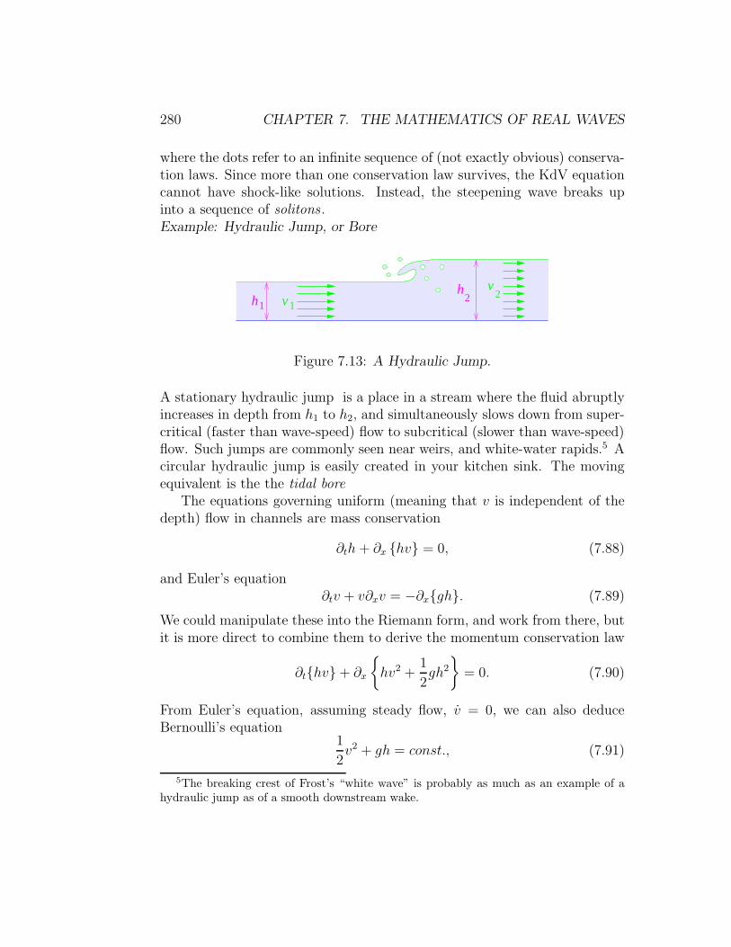
280 CHAPTER 7. THE MATHEMATICS OF REAL WAVES
where the dots refer to an infinite sequence of (not exactly obvious) conserva-tion laws. Since more than one conservation law survives, the KdV equationcannot have shock-like solutions. Instead, the steepening wave breaks upinto a sequence of solitons .Example: Hydraulic Jump, or Bore
v1
v2
h1
h2
Figure 7.13: A Hydraulic Jump.
A stationary hydraulic jump is a place in a stream where the fluid abruptlyincreases in depth from h1 to h2, and simultaneously slows down from super-critical (faster than wave-speed) flow to subcritical (slower than wave-speed)flow. Such jumps are commonly seen near weirs, and white-water rapids.5 Acircular hydraulic jump is easily created in your kitchen sink. The movingequivalent is the the tidal bore
The equations governing uniform (meaning that v is independent of thedepth) flow in channels are mass conservation
∂th + ∂x hv = 0, (7.88)
and Euler’s equation∂tv + v∂xv = −∂xgh. (7.89)
We could manipulate these into the Riemann form, and work from there, butit is more direct to combine them to derive the momentum conservation law
∂thv+ ∂x
hv2 +
1
2gh2
= 0. (7.90)
From Euler’s equation, assuming steady flow, v = 0, we can also deduceBernoulli’s equation
1
2v2 + gh = const., (7.91)
5The breaking crest of Frost’s “white wave” is probably as much as an example of ahydraulic jump as of a smooth downstream wake.
7.3. NON-LINEAR WAVES 281
which is an energy conservation law. At the jump, mass and momentummust be conserved:
h1v1 = h2v2,
h1v21 +
1
2gh21 = h2v
22 +
1
2gh22, (7.92)
and v2 may be eliminated to find
v21 =1
2g
(h2h1
)(h1 + h2). (7.93)
A change of frame reveals that v1 is the speed at which a wall of water ofheight h = (h2 − h1) would propagate into stationary water of depth h1.
Bernoulli’s equation is inconsistent with the two equations we have used,and so
1
2v21 + gh1 6=
1
2v22 + gh2. (7.94)
This means that energy is being dissipated: for strong jumps, the fluid down-stream is turbulent. For weaker jumps, the energy is radiated away in a trainof waves – the so-called “undular bore”.Example: Shock Wave in Air: At a shock wave in air we have conservationof mass
ρ1v1 = ρ2v2, (7.95)
and momentumρ1v
21 + P1 = ρ2v
22 + P2. (7.96)
In this case, however, Bernoulli’s equation does hold,6, so we also have
1
2v21 + h1 =
1
2v22 + h2. (7.97)
Here, h is the specific enthalpy (U +PV per unit mass). Entropy, though, isnot conserved, so we cannot use PV γ = const. across the shock. From mass
6Recall that enthalpy is conserved in a throttling process even in the presence of dissi-pation. Bernoulli’s equation for a gas is the generalization of this thermodynamic result toinclude the kinetic energy of the gas. The difference between the shock wave in air, whereBernoulli holds, and the hydraulic jump, where it does not, is that the enthalpy of the gaskeeps track of the lost mechanical energy, which has been absorbed by the internal degreesof freedom. The Bernoulli equation for channel flow keeps track only of the mechanicalenergy of the mean flow.

282 CHAPTER 7. THE MATHEMATICS OF REAL WAVES
and momentum conservation alone we find
v21 =
(ρ2ρ1
)P2 − P1
ρ2 − ρ1. (7.98)
For an ideal gas with cp/cv = γ, we can use energy conservation to to elimi-nate the densities, and find
v1 = c0
√1 +
γ + 1
2γ
P2 − P1
P1. (7.99)
Here, c0 is the speed of sound in the undisturbed gas.
7.3.3 Weak Solutions
We want to make mathematically precise the sense in which a function uwith a discontinuity can be a solution to the differential equation
∂t
1
nun+ ∂x
1
n + 1un+1
= 0, (7.100)
even though the equation is surely meaningless if the functions to which thederivatives are being applied are not in fact differentiable.
We could play around with distributions like the Heaviside step functionor the Dirac delta, but this is unsafe for non-linear equations, because theproduct of two distributions is generally not meaningful. What we do isintroduce a new concept. We say that u is a weak solution to (7.100) if
∫
R2
dx dt
un∂tϕ+
n
n + 1un+1∂xϕ
= 0, (7.101)
for all test functions ϕ in some suitable space T . This equation has formallybeen obtained from (7.100) by multiplying it by ϕ(x, t), integrating overall space-time, and then integrating by parts to move the derivatives off u,and onto the smooth function ϕ. If u is assumed smooth then all thesemanipulations are legitimate and the new equation (7.101) contains no newinformation. A conventional solution to (7.100) is therefore also a weaksolution. The new formulation (7.101), however, admits solutions in which uhas shocks.

7.3. NON-LINEAR WAVES 283
x
tX(t)
D− D+
n
Figure 7.14: The geometry of the domains to the right and left of a jump.
Let us see what is required of a weak solution if we assume that u iseverywhere smooth except for a single jump from u−(t) to u+(t) at the pointX(t). Let D± be the regions to the left and right of the jump, as shown infigure 7.14. Then the weak-solution condition (7.101) becomes
0 =
∫
D−
dx dt
un∂tϕ+
n
n+ 1un+1∂xϕ
+
∫
D+
dx dt
un∂tϕ+
n
n+ 1un+1∂xϕ
.
(7.102)Let
n =
1√
1 + |X|2,−X√1 + |X|2
(7.103)
be the unit outward normal to D−, then, using the divergence theorem, wehave∫
D−
dx dt
un∂tϕ+
n
n+ 1un+1∂xϕ
=
∫
D−
dx dt
−ϕ
(∂tu
n +n
n+ 1∂xu
n+1
)
+
∫
∂D−
dt
ϕ
(−X(t)un− +
n
n + 1un+1−
)
(7.104)
Here we have written the integration measure over the boundary as
ds =
√1 + |X|2 dt. (7.105)
Performing the same manoeuvre for D+, and observing that ϕ can be anysmooth function, we deduce that

284 CHAPTER 7. THE MATHEMATICS OF REAL WAVES
i) ∂tun + n
n+1∂xu
n+1 = 0 within D±.
ii) X(un+ − un−) = nn+1
(un+1+ − un+1
− ) on X(t).The reasoning here is identical to that in chapter one, where we consideredvariations at endpoints to obtain natural boundary conditions. We thereforeend up with the same equations for the motion of the shock as before.
The notion of weak solutions is widely used in applied mathematics, and itis the principal ingredient of the finite element method of numerical analysisin continuum dynamics.
7.4 Solitons
A localized disturbance in a dispersive medium soon falls apart, since itsvarious frequency components travel at differing speeds. At the same time,non-linear effects will distort the wave profile. In some systems, however,these effects of dispersion and non-linearity can compensate each other andgive rise to solitons—stable solitary waves which propagate for long distanceswithout changing their form. Not all equations possessing wave-like solutionsalso possess solitary wave solutions. The best known example of equationsthat do, are:
1) The Korteweg-de-Vries (KdV) equation, which in the form
∂u
∂t+ u
∂u
∂x= −∂
3u
∂x3, (7.106)
has a solitary wave solution
u(x, t) = 3α2sech2
1
2(αx− α3t)
(7.107)
which travels at speed α2. The larger the amplitude, therefore, thefaster the solitary wave travels. This equation applies to steep wavesin shallow water.
2) The non-linear Shrodinger (NLS) equation with attractive interactions
i∂ψ
∂t= − 1
2m
∂2ψ
∂x2− λ|ψ|2ψ, (7.108)
where λ > 0. It has solitary-wave solution
ψ = eikx−iωt√
α
mλsech√α(x− Ut), (7.109)

7.4. SOLITONS 285
where
k = mU, ω =1
2mU2 − α
2m. (7.110)
In this case, the speed is independent of the amplitude, and the movingsolution can be obtained from a stationary one by means of a Galileanboost. The nonlinear equation for the stationary wavepacket may besolved by observing that
(−∂2x − 2sech2x)ψ0 = −ψ0 (7.111)
where ψ0(x) = sech x. This is the bound-state of the Poschel-Tellerequation that we have met several times before. The non-linear Schrodingerequation describes many systems, including the dynamics of tornadoes,where the solitons manifest as the knot-like kinks sometimes seen wind-ing their way up thin funnel clouds.7
3) The sine-Gordon (SG) equation is
∂2ϕ
∂t2− ∂2ϕ
∂x2+m2
βsin βϕ = 0. (7.112)
This has solitary-wave solutions
ϕ(x, t) =4
βtan−1
e±mγ(x−Ut)
, (7.113)
where γ = (1 − U2)−12 and |U | < 1. The velocity is not related to the
amplitude, and the moving soliton can again be obtained by boostinga stationary soliton. The boost is now a Lorentz transformation, andso we only get subluminal solitons, whose width is Lorentz contractedby the usual relativistic factor of γ. The sine-Gordon equation de-scribes, for example, the evolution of light pulses whose frequency is inresonance with an atomic transition in the propagation medium.8
In the case of the sine-Gordon soliton, the origin of the solitary wave isparticularly easy to understand, as it can be realized as a “twist” in a chainof coupled pendulums. The handedness of the twist determines whether wetake the + or − sign in the solution (7.113).
7H.Hasimoto, J. Fluid Mech. 51 (1972) 477-485.8See G. L. Lamb, Rev. Mod. Phys. 43(1971) 99, for a nice review.

286 CHAPTER 7. THE MATHEMATICS OF REAL WAVES
Figure 7.15: A sine-Gordon solitary wave as a twist in a ribbon of coupledpendulums.
The existence of solitary-wave solutions is interesting in its own right.It was the fortuitous observation of such a wave by John Scott Russell onthe Union Canal, near Hermiston in Scotland, that founded the subject.9
Even more remarkable was Scott Russell’s subsequent discovery (made in aspecially constructed trough in his garden) of what is now called the solitonproperty : two colliding solitary waves interact in a complicated manner yetemerge from the encounter with their form unchanged, having suffered nomore than a slight time delay. Each of the three equations given above hasexact multi-soliton solutions which show this phenomenon.
After languishing for more than a century, soliton theory has grown tobe a huge subject. It is, for example, studied by electrical engineers whouse soliton pulses in fibre-optic communications. No other type of signalcan propagate though thousands of kilometers of undersea cable withoutdegradation. Solitons, or “quantum lumps” are also important in particlephysics. The nucleon can be thought of as a knotted soliton (in this casecalled a “skyrmion”) in the pion field, and gauge-field monopole solitons
9“I was observing the motion of a boat which was rapidly drawn along a narrow channelby a pair of horses, when the boat suddenly stopped - not so the mass of water in thechannel which it had put in motion; it accumulated round the prow of the vessel in a stateof violent agitation, then suddenly leaving it behind, rolled forward with great velocity,assuming the form of a large solitary elevation, a rounded, smooth and well-defined heapof water, which continued its course along the channel apparently without change of formor diminution of speed. I followed it on horseback, and overtook it still rolling on at a rateof some eight or nine miles an hour, preserving its original figure some thirty feet long anda foot to a foot and a half in height. Its height gradually diminished, and after a chase ofone or two miles I lost it in the windings of the channel. Such, in the month of August1834, was my first chance interview with that singular and beautiful phenomenon which Ihave called the Wave of Translation.” —John Scott Russell, 1844.

7.4. SOLITONS 287
appear in many string and field theories. The soliton equations themselvesare aristocrats among partial differential equations, with ties into almostevery other branch of mathematics.Practical Illustration: Solitons in Optical Fibres. We wish to transmit pi-cosecond pulses of light with a carrier frequency ω0. Suppose that the dis-persive properties of the fibre are such that the associated wavenumber forfrequencies near ω0 can be expanded as
k = ∆k + k0 + β1(ω − ω0) +1
2β2(ω − ω0)
2 + · · · . (7.114)
Here, β1 is the reciprocal of the group velocity, and β2 is a parameter calledthe group velocity dispersion (GVD). The term ∆k parameterizes the changein refractive index due to non-linear effects. It is proportional to the mean-square of the electric field. Let us write the electric field as
E(x, t) = A(x, t)eik0z−ω0t, (7.115)
where A(x, t) is a slowly varying envelope function. When we transform fromFourier variables to space and time we have
(ω − ω0)→ i∂
∂t, (k − k0)→ −i
∂
∂z, (7.116)
and so the equation determining A becomes
−i∂A∂z
= iβ1∂A
∂t− β2
2
∂2A
∂t2+∆kA. (7.117)
If we set ∆k = γ|A2|, where γ is normally positive, we have
i
(∂A
∂z+ β1
∂A
∂t
)=β22
∂2A
∂t2− γ|A|2A. (7.118)
We may get rid of the first-order time derivative by transforming to a framemoving at the group velocity. We do this by setting
τ = t− β1z,ζ = z (7.119)
and using the chain rule, as we did for the Galilean transformation in home-work set 0. The equation for A ends up being
i∂A
∂ζ=β22
∂2A
∂τ 2− γ|A|2A. (7.120)
288 CHAPTER 7. THE MATHEMATICS OF REAL WAVES
This looks like our non-linear Schrodinger equation, but with the role ofspace and time interchanged! Also, the coefficient of the second derivativehas the wrong sign so, to make it coincide with the Schrodinger equation westudied earlier, we must have β2 < 0. When this condition holds, we aresaid to be in the “anomalous dispersion” regime — although this is rathera misnomer since it is the group refractive index , Ng = c/vgroup, that isdecreasing with frequency, not the ordinary refractive index. For pure SiO2
glass, β2 is negative for wavelengths greater than 1.27µm. We therefore haveanomalous dispersion in the technologically important region near 1.55µm,where the glass is most transparent. In the anomalous dispersion regime wehave solitons with
A(ζ, τ) = eiα|β2|ζ/2
√β2α
γsech√α(τ), (7.121)
leading to
E(z, t) =
√β2α
γsech√α(t− β1z)eiα|β2|z/2eik0z−iω0t. (7.122)
This equation describes a pulse propagating at β−11 , which is the group ve-
locity.
Exercise 7.1: Find the expression for the sine-Gordon soliton, by first showingthat the static sine-Gordon equation
−∂2ϕ
∂x2+m2
βsin βϕ = 0
implies that1
2ϕ′2 +
m2
β2cos βϕ = const.,
and solving this equation (for a suitable choice of the constant) by separationof variables. Next, show that if f(x) is solution of the static equation, thenf(γ(x − Ut)), γ = (1 − U2)−1/2, |U | < 1 is a solution of the time-dependentequation.
Exercise 7.2: Lax pair for the non-linear Schrodinger equation. Let L be thematrix differential operator
L =
[i∂x χ∗
χ i∂x
],

7.5. FURTHER EXERCISES AND PROBLEMS 289
and let P be the matrix
P =
[i|χ|2 −χ′∗
χ′ −i|χ|2].
Show that the equation
L = [L,P ]
is equivalent to the non-linear Shrodinger equation
iχ = −χ′′ − 2|χ|2χ.
7.5 Further Exercises and Problems
Here are some further problems on non-linear and dispersive waves:
Problem 7.3: The Equation of Telegraphy . Oliver Heaviside’s equations re-lating the voltage v(x, t) and current i(x, t) in a transmission line are
L∂i
∂t+Ri = −∂v
∂x,
C∂v
∂t+Gv = − ∂i
∂x.
Here R, C, L and G are respectively the resitance, capacitance, inductance,and leakance of each unit length of the line.
a) Show that Heaviside’s equations lead to v(x, t) obeying
LC∂2v
∂t2+ (LG+RC)
∂v
∂t+RGv =
∂2v
∂x2,
and also to a similar equation for i(x, t).b) Seek a travelling-wave solution of the form
v(x, t) = v0 ei(kx+ωt),
i(x, t) = i0 ei(kx+ωt),
and find the dispersion equation relating ω and k. From this relation,show that signals propagate undistorted (i.e. with frequency-independentattenuation) at speed 1/
√LC provided that the Heaviside condition
RC = LG is satisfied.
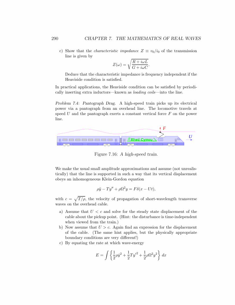
290 CHAPTER 7. THE MATHEMATICS OF REAL WAVES
c) Show that the characteristic impedance Z ≡ v0/i0 of the transmissionline is given by
Z(ω) =
√R+ iωL
G+ iωC.
Deduce that the characteristic impedance is frequency independent if theHeaviside condition is satisfied.
In practical applications, the Heaviside condition can be satisfied by periodi-cally inserting extra inductors—known as loading coils—into the line.
Problem 7.4: Pantograph Drag. A high-speed train picks up its electricalpower via a pantograph from an overhead line. The locomotive travels atspeed U and the pantograph exerts a constant vertical force F on the powerline.
F
URheil Cymru
Figure 7.16: A high-speed train.
We make the usual small amplitude approximations and assume (not unrealis-tically) that the line is supported in such a way that its vertical displacementobeys an inhomogeneous Klein-Gordon equation
ρy − Ty′′ + ρΩ2y = Fδ(x − Ut),
with c =√T/ρ, the velocity of propagation of short-wavelength transverse
waves on the overhead cable.
a) Assume that U < c and solve for the steady state displacement of thecable about the pickup point. (Hint: the disturbance is time-independentwhen viewed from the train.)
b) Now assume that U > c. Again find an expression for the displacementof the cable. (The same hint applies, but the physically appropriateboundary conditions are very different!)
c) By equating the rate at which wave-energy
E =
∫ 1
2ρy2 +
1
2Ty′2 +
1
2ρΩ2y2
dx
7.5. FURTHER EXERCISES AND PROBLEMS 291
is being created to rate at the which the locomotive is doing work, cal-culate the wave-drag on the train. In particular, show that there is nodrag at all until U exceeds c. (Hint: While the front end of the wake ismoving at speed U , the trailing end of the wake is moving forward at thegroup velocity of the wave-train.)
d) By carefully considering the force the pantograph exerts on the overheadcable, again calculate the induced drag. You should get the same answeras in part c) (Hint: To the order needed for the calculation, the tensionin the cable is the same before and after the train has passed, but thedirection in which the tension acts is different. The force F is thereforenot exactly vertical, but has a small forward component. Don’t forgetthat the resultant of the forces is accelerating the cable.)
This problem of wake formation and drag is related both to Cerenkov radiationand to the Landau criterion for superfluidity.
Exercise 7.5: Inertial waves. A rotating tank of incompressible (ρ ≡ 1) fluidcan host waves whose restoring force is provided by angular momentum con-servation. Suppose the fluid velocity at the point r is given by
v(r, t) = u(r, t) +Ω× r,
where u is a perturbation imposed on the rigid rotation of the fluid at angularvelocity Ω.
a) Show that when viewed from a co-ordinate frame rotating with the fluidwe have
∂u
∂t=
(∂u
∂t−Ω× u+ ((Ω × r) · ∇)u
)
lab
.
Deduce that the lab-frame Euler equation
∂v
∂t+ (v · ∇)v = −∇P,
becomes, in the rotating frame,
∂u
∂t+ 2(Ω × u) + (u · ∇)u = −∇
(P − 1
2|Ω× r|2
).
We see that in the non-inertial rotating frame the fluid experiences a−2(Ω × u) Coriolis and a ∇|Ω × r|2/2 centrifugal force. By linearizingthe rotating-frame Euler equation, show that for small u we have
∂ω
∂t− 2(Ω · ∇)u = 0, (⋆)
where ω = curlu.

292 CHAPTER 7. THE MATHEMATICS OF REAL WAVES
b) Take Ω to be directed along the z axis. Seek plane-wave solutions to ⋆in the form
u(r, t) = uoei(k·r−ωt)
where u0 is a constant, and show that the dispersion equation for thesesmall amplitude inertial waves is
ω = 2Ω
√k2z
k2x + k2y + k2z.
Deduce that the group velocity is directed perpendicular to k— i.e. atright-angles to the phase velocity. Conclude also that any slow flowthat is steady (time independent) when viewed from the rotating frameis necessarily independent of the co-ordinate z. (This is the origin ofthe phenomenon of Taylor columns, which are columns of stagnant fluidlying above and below any obstacle immersed in such a flow.)
Exercise 7.6: Non-linear Waves. In this problem we will explore the Riemanninvariants for a fluid with P = λ2ρ3/3. This is the equation of state of one-dimensional non-interacting Fermi gas.
a) From the continuity equation
∂tρ+ ∂xρv = 0,
and Euler’s equation of motion
ρ(∂tv + v∂xv) = −∂xP,
deduce that(∂
∂t+ (λρ+ v)
∂
∂x
)(λρ+ v) = 0,
(∂
∂t+ (−λρ+ v)
∂
∂x
)(−λρ+ v) = 0.
In what limit do these equations become equivalent to the wave equationfor one-dimensional sound? What is the sound speed in this case?
b) Show that the Riemann invariants v±λρ are constant on suitably definedcharacteristic curves. What is the local speed of propagation of the wavesmoving to the right or left?
c) The fluid starts from rest, v = 0, but with a region where the densityis higher than elsewhere. Show that that the Riemann equations willinevitably break down at some later time due to the formation of shockwaves.

7.5. FURTHER EXERCISES AND PROBLEMS 293
Exercise 7.7: Burgers Shocks. As simple mathematical model for the forma-tion and decay of a shock wave consider Burgers’ Equation:
∂tu+ u∂xu = ν ∂2xu.
Note its similarity to the Riemann equations of the previous exercise. Theadditional term on the right-hand side introduces dissipation and prevents thesolution becoming multi-valued.
a) Show that if ν = 0 any solution of Burgers’ equation having a regionwhere u decreases to the right will always eventually become multivalued.
b) Show that the Hopf-Cole transformation, u = −2ν ∂x lnψ, leads to ψobeying a heat diffusion equation
∂tψ = ν ∂2xψ.
c) Show that
ψ(x, t) = Aeνa2t−ax +Beνb
2t−bx
is a solution of this heat equation, and so deduce that Burgers’ equationhas a shock-wave-like solution which travels to the right at speed C =ν(a+ b) = 1
2(uL+uR), the mean of the wave speeds to the left and rightof the shock. Show that the width of the shock is ≈ 4ν/|uL − uR|.

294 CHAPTER 7. THE MATHEMATICS OF REAL WAVES

Chapter 8
Special Functions
In solving Laplace’s equation by the method of separation of variables wecome across the most important of the special functions of mathematicalphysics. These functions have been studied for many years, and books such asthe Bateman manuscript project1 summarize the results. Any serious studenttheoretical physics needs to be familiar with this material, and should at leastread the standard text: A Course of Modern Analysis by E. T. Whittakerand G. N. Watson (Cambridge University Press). Although it was originallypublished in 1902, nothing has superseded this book in its accessibility andusefulness.
In this chapter we will focus only on the properties that all physics stu-dents should know by heart.
8.1 Curvilinear Co-ordinates
Laplace’s equation can be separated in a number of coordinate systems.These are all orthogonal systems in that the local coordinate axes cross atright angles.
1The Bateman manuscript project contains the formulæ collected by Harry Bateman,who was professor of Mathematics, Theoretical Physics, and Aeronautics at the CaliforniaInstitute of Technology. After his death in 1946, several dozen shoe boxes full of file cardswere found in his garage. These proved to be the index to a mountain of paper contain-ing his detailed notes. A subset of the material was eventually published as the threevolume series Higher Transcendental Functions , and the two volume Tables of IntegralTransformations , A. Erdelyi et al. eds.
295

296 CHAPTER 8. SPECIAL FUNCTIONS
To any system of orthogonal curvilinear coordinates is associated a metricof the form
ds2 = h21(dx1)2 + h22(dx
2)2 + h23(dx3)2. (8.1)
This expression tells us the distance√ds2 between the adjacent points
(x1 + dx1, x2 + dx2, x3 + dx3) and (x1, x2, x3). In general, the hi will dependon the co-ordinates xi.
The most commonly used orthogonal curvilinear co-ordinate systems areplane polars, spherical polars, and cylindrical polars. The Laplacian alsoseparates in plane elliptic, or three-dimensional ellipsoidal coordinates andtheir degenerate limits, such as parabolic cylindrical co-ordinates — but theseare not so often encountered, and for their properties we refer the reader tocomprehensive treatises such as Morse and Feshbach’s Methods of TheoreticalPhysics.
Plane Polar Co-ordinates
θ
P
y
x
r
Figure 8.1: Plane polar co-ordinates.
Plane polar co-ordinates have metric
ds2 = dr2 + r2dθ2, (8.2)
so hr = 1, hθ = r.

8.1. CURVILINEAR CO-ORDINATES 297
Spherical Polar Co-ordinates
x
y
z
P
θ
r
φ
Figure 8.2: Spherical co-ordinates.
This system has metric
ds2 = dr2 + r2dθ2 + r2 sin2 θdφ2, (8.3)
so hr = 1, hθ = r, hφ = r sin θ,
Cylindrical Polar Co-ordinates
x
y
z
Pr
z
θ
Figure 8.3: Cylindrical co-ordinates.
These have metricds2 = dr2 + r2dθ2 + dz2, (8.4)
so hr = 1, hθ = r, hz = 1.
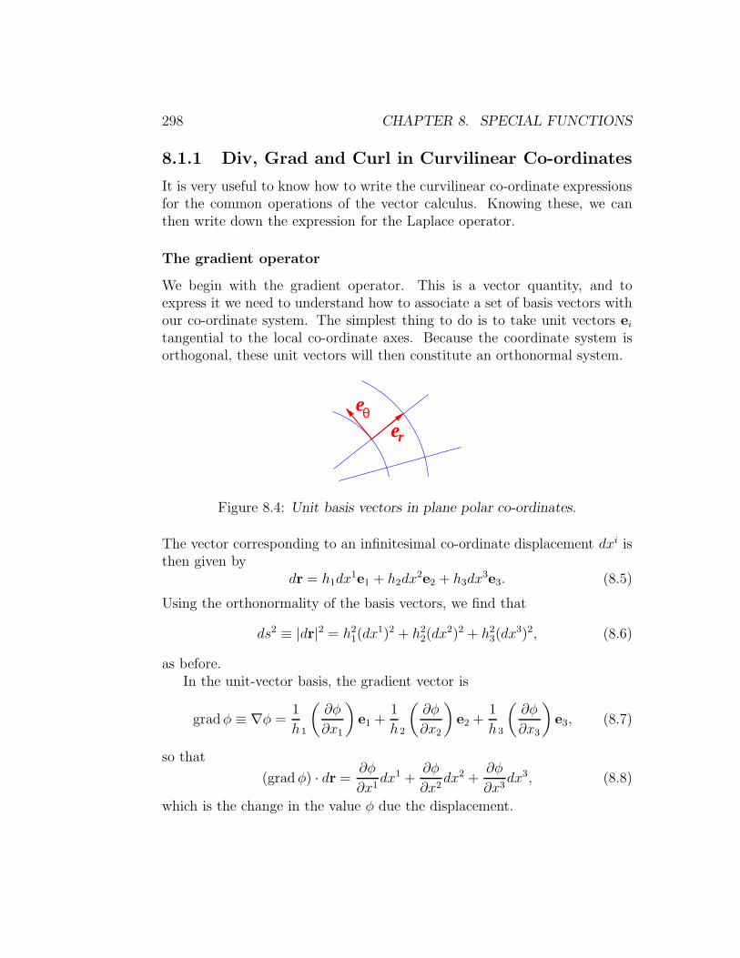
298 CHAPTER 8. SPECIAL FUNCTIONS
8.1.1 Div, Grad and Curl in Curvilinear Co-ordinates
It is very useful to know how to write the curvilinear co-ordinate expressionsfor the common operations of the vector calculus. Knowing these, we canthen write down the expression for the Laplace operator.
The gradient operator
We begin with the gradient operator. This is a vector quantity, and toexpress it we need to understand how to associate a set of basis vectors withour co-ordinate system. The simplest thing to do is to take unit vectors eitangential to the local co-ordinate axes. Because the coordinate system isorthogonal, these unit vectors will then constitute an orthonormal system.
ee
r
θ
Figure 8.4: Unit basis vectors in plane polar co-ordinates.
The vector corresponding to an infinitesimal co-ordinate displacement dxi isthen given by
dr = h1dx1e1 + h2dx
2e2 + h3dx3e3. (8.5)
Using the orthonormality of the basis vectors, we find that
ds2 ≡ |dr|2 = h21(dx1)2 + h22(dx
2)2 + h23(dx3)2, (8.6)
as before.In the unit-vector basis, the gradient vector is
gradφ ≡ ∇φ =1
h1
(∂φ
∂x1
)e1 +
1
h 2
(∂φ
∂x2
)e2 +
1
h3
(∂φ
∂x3
)e3, (8.7)
so that
(gradφ) · dr = ∂φ
∂x1dx1 +
∂φ
∂x2dx2 +
∂φ
∂x3dx3, (8.8)
which is the change in the value φ due the displacement.
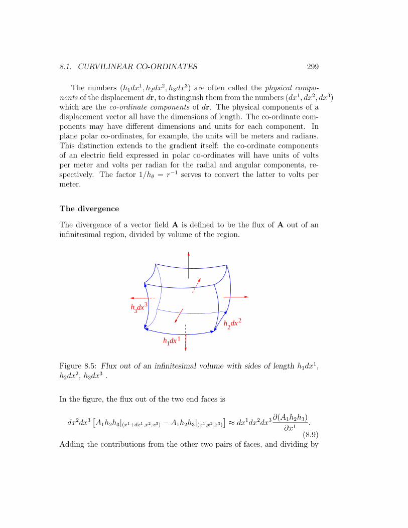
8.1. CURVILINEAR CO-ORDINATES 299
The numbers (h1dx1, h2dx
2, h3dx3) are often called the physical compo-
nents of the displacement dr, to distinguish them from the numbers (dx1, dx2, dx3)which are the co-ordinate components of dr. The physical components of adisplacement vector all have the dimensions of length. The co-ordinate com-ponents may have different dimensions and units for each component. Inplane polar co-ordinates, for example, the units will be meters and radians.This distinction extends to the gradient itself: the co-ordinate componentsof an electric field expressed in polar co-ordinates will have units of voltsper meter and volts per radian for the radial and angular components, re-spectively. The factor 1/hθ = r−1 serves to convert the latter to volts permeter.
The divergence
The divergence of a vector field A is defined to be the flux of A out of aninfinitesimal region, divided by volume of the region.
dx
dx
3
1
3
1h
h22
dxh
Figure 8.5: Flux out of an infinitesimal volume with sides of length h1dx1,
h2dx2, h3dx
3 .
In the figure, the flux out of the two end faces is
dx2dx3[A1h2h3|(x1+dx1,x2,x3) − A1h2h3|(x1,x2,x3)
]≈ dx1dx2dx3
∂(A1h2h3)
∂x1.
(8.9)Adding the contributions from the other two pairs of faces, and dividing by

300 CHAPTER 8. SPECIAL FUNCTIONS
the volume, h2h2h3dx1dx2dx3, gives
divA =1
h1h2h3
∂
∂x1(h2h3A1) +
∂
∂x2(h1h3A2) +
∂
∂x3(h1h2A3)
. (8.10)
Note that in curvilinear coordinates divA is no longer simply ∇·A, althoughone often writes it as such.
The curl
The curl of a vector field A is a vector whose component in the direction ofthe normal to an infinitesimal area element, is line integral of A round theinfinitesimal area, divided by the area.
h dx
h dx
e
1
2
3
1
2
Figure 8.6: Line integral round infinitesimal area with sides of length h1dx1,
h2dx2, and normal e3 .
The third component is, for example,
(curlA)3 =1
h1h2
(∂h2A2
∂x1− ∂h1A1
∂x2
). (8.11)
The other two components are found by cyclically permuting 1→ 2→ 3→ 1in this formula. The curl is thus is no longer equal to ∇×A, although it iscommon to write it as if it were.
Note that the factors of hi are disposed so that the vector identities
curl gradϕ = 0, (8.12)
anddiv curlA = 0, (8.13)
continue to hold for any scalar field ϕ, and any vector field A.

8.1. CURVILINEAR CO-ORDINATES 301
8.1.2 The Laplacian in Curvilinear Co-ordinates
The Laplacian acting on scalars, is “div grad”, and is therefore
∇2ϕ =1
h1h2h3
∂
∂x1
(h2h3h1
∂ϕ
∂x1
)+
∂
∂x2
(h1h3h2
∂ϕ
∂x2
)+
∂
∂x3
(h1h2h3
∂ϕ
∂x3
).
(8.14)This formula is worth committing to memory.
When the Laplacian is to act on a vector field , we must use the vectorLaplacian
∇2A = grad divA− curl curlA. (8.15)
In curvilinear co-ordinates this is no longer equivalent to the Laplacian actingon each component of A, treating it as if it were a scalar. The expression(8.15) is the appropriate generalization of the vector Laplacian to curvilinearco-ordinates because it is defined in terms of the co-ordinate independentoperators div, grad, and curl, and reduces to the Laplacian on the individualcomponents when the co-ordinate system is Cartesan.
In spherical polars the Laplace operator acting on the scalar field ϕ is
∇2ϕ =1
r2∂
∂r
(r2∂ϕ
∂r
)+
1
r2 sin θ
∂
∂θ
(sin θ
∂ϕ
∂θ
)+
1
r2 sin2 θ
∂2ϕ
∂φ2
=1
r
∂2(rϕ)
∂r2+
1
r2
1
sin θ
∂
∂θ
(sin θ
∂ϕ
∂θ
)+
1
sin2 θ
∂2ϕ
∂φ2
=1
r
∂2(rϕ)
∂r2− L2
r2ϕ, (8.16)
where
L2 = − 1
sin θ
∂
∂θsin θ
∂
∂θ− 1
sin2 θ
∂2
∂φ2, (8.17)
is (after multiplication by ~2) the operator representing the square of theangular momentum in quantum mechanics.
In cylindrical polars the Laplacian is
∇2ϕ =1
r
∂
∂rr∂ϕ
∂r+
1
r2∂2ϕ
∂θ2+∂2ϕ
∂z2. (8.18)

302 CHAPTER 8. SPECIAL FUNCTIONS
8.2 Spherical Harmonics
We saw that Laplace’s equation in spherical polars is
0 =1
r
∂2(rϕ)
∂r2− L2
r2ϕ. (8.19)
To solve this by the method of separation of variables, we factorize
ϕ = R(r)Y (θ, φ), (8.20)
so that1
Rr
d2(rR)
dr2− 1
r2
(1
YL2Y
)= 0. (8.21)
Taking the separation constant to be l(l + 1), we have
rd2(rR)
dr2− l(l + 1)(rR) = 0, (8.22)
andL2Y = l(l + 1)Y. (8.23)
The solution for R is rl or r−l−1. The equation for Y can be further decom-posed by setting Y = Θ(θ)Φ(φ). Looking back at the definition of L2, we seethat we can take
Φ(φ) = eimφ (8.24)
with m an integer to ensure single valuedness. The equation for Θ is then
1
sin θ
d
dθ
(sin θ
dΘ
dθ
)− m2
sin2 θΘ = −l(l + 1)Θ. (8.25)
It is convenient to set x = cos θ; then(d
dx(1− x2) d
dx+ l(l + 1)− m2
1− x2)Θ = 0. (8.26)
8.2.1 Legendre Polynomials
We first look at the axially symmetric case where m = 0. We are left with(d
dx(1− x2) d
dx+ l(l + 1)
)Θ = 0. (8.27)

8.2. SPHERICAL HARMONICS 303
This is Legendre’s equation. We can think of it as an eigenvalue problem
−(d
dx(1− x2) d
dx
)Θ(x) = l(l + 1)Θ(x), (8.28)
on the interval −1 ≤ x ≤ 1, this being the range of cos θ for real θ. Legendre’sequation is of Sturm-Liouville form, but with regular singular points at x =±1. Because the endpoints of the interval are singular, we cannot imposeas boundary conditions that Θ, Θ′, or some linear combination of these, bezero there. We do need some boundary conditions, however, so as to have aself-adjoint operator and a complete set of eigenfunctions.
Given one or more singular endpoints, a possible route to a well-definedeigenvalue problem is to require solutions to be square-integrable, and sonormalizable. This condition suffices for the harmonic-oscillator Schrodingerequation, for example, because at most one of the two solutions is square-integrable. For Legendre’s equation with l = 0, the two independent solutionsare Θ(x) = 1 and Θ(x) = ln(1 + x)− ln(1− x). Both of these solutions havefinite L2[−1, 1] norms, and this square integrability persists for all values ofl. Thus, demanding normalizability is not enough to select a unique bound-ary condition. Instead, each endpoint possesses a one-parameter family ofboundary conditions that lead to self-adjoint operators. We therefore makethe more restrictive demand that the allowed eigenfunctions be finite at theendpoints. Because the the north and south pole of the sphere are not specialpoints, this is a physically reasonable condition. When l is an integer, thenone of the solutions, Pl(x), becomes a polynomial, and so is finite at x = ±1.The second solution Ql(x) is divergent at both ends, and so is not an allowedsolution. When l is not an integer, neither solution is finite. The eigenvaluesare therefore l(l + 1) with l zero or a positive integer. Despite its unfa-miliar form, the “finite” boundary condition makes the Legendre operatorself-adjoint, and the Legendre polynomials Pl(x) form a complete orthogonalset for L2[−1, 1].
Proving orthogonality is easy: we follow the usual strategy for Sturm-Liouville equations with non-singular boundary conditions to deduce that
[l(l + 1)−m(m+ 1)]
∫ 1
−1
Pl(x)Pm(x) dx =[(PlP
′m − P ′
lPm)(1− x2)]1−1.
(8.29)Since the Pl’s remain finite at ±1, the right hand side is zero because of the(1 − x2) factor, and so
∫ 1
−1Pl(x)Pm(x) dx is zero if l 6= m. (Observe that
304 CHAPTER 8. SPECIAL FUNCTIONS
this last step differs from the usual argument where it is the vanishing of theeigenfunction or its derivative that makes the integrated-out term zero.)
Because they are orthogonal polynomials, the Pl(x) can be obtained byapplying the Gram-Schmidt procedure to the sequence 1, x, x2, . . . to obtainpolynomials orthogonal with respect to the w ≡ 1 inner product, and thenfixing the normalization constant. The result of this process can be expressedin closed form as
Pl(x) =1
2ll!
dl
dxl(x2 − 1)l. (8.30)
This is called Rodriguez’ formula. It should be clear that this formula outputsa polynomial of degree l. The coefficient 1/2ll! comes from the traditionalnormalization for the Legendre polynomials that makes Pl(1) = 1. Thisconvention does not lead to an orthonormal set. Instead, we have
∫ 1
−1
Pl(x)Pm(x) dx =2
2l + 1δlm. (8.31)
It is easy to show that this integral is zero if l > m—simply integrate byparts l times so as to take the l derivatives off (x2 − 1)l and onto (x2 − 1)m,which they kill. We will evaluate the l = m integral in the next section.
We now show that the Pl(x) given by Rodriguez formula are indeed so-lutions of Legendre’s equation: Let v = (x2 − 1)l, then
(1− x2)v′ + 2lxv = 0. (8.32)
We differentiate this l + 1 times using Leibniz’ theorem
[uv](n) =
n∑
m=0
(n
m
)u(m)v(n−m)
= uv(n) + nu′v(n−1) +1
2n(n− 1)u′′v(n−2) + . . . . (8.33)
We find that
[(1− x2)v′](l+1) = (1− x2)v(l+2) − (l + 1)2xv(l+1) − l(l + 1)v(l),
[2xnv](l+1) = 2xlv(l+1) + 2l(l + 1)v(l). (8.34)
Putting these two terms together we obtain((1− x2) d
2
dx2− 2x
d
dx+ l(l + 1)
)dl
dxl(x2 − 1)l = 0, (8.35)

8.2. SPHERICAL HARMONICS 305
which is Legendre’s equation.The Pl(x) have alternating parity
Pl(−x) = (−1)lPl(x), (8.36)
and the first few are
P0(x) = 1,
P1(x) = x,
P2(x) =1
2(3x2 − 1),
P3(x) =1
2(5x3 − 3x),
P4(x) =1
8(35x4 − 30x2 + 3).
8.2.2 Axisymmetric potential problems
The essential property of the Pl(x) is that the general axisymmetric solutionof ∇2ϕ = 0 can be expanded in terms of them as
ϕ(r, θ) =
∞∑
l=0
(Alr
l +Blr−l−1
)Pl(cos θ). (8.37)
You should memorize this formula. You should also know by heart the ex-plicit expressions for the first four Pl(x), and the factor of 2/(2l + 1) in theorthogonality formula.Example: Point charge. Put a unit charge at the point R, and find an ex-pansion for the potential as a Legendre polynomial series in a neighbourhoodof the origin.
R
|
θ
r
R−r |
O
Figure 8.7: Geometry for generating function.

306 CHAPTER 8. SPECIAL FUNCTIONS
Let start by assuming that |r| < |R|. We know that in this region the pointcharge potential 1/|r−R| is a solution of Laplace’s equation , and so we canexpand
1
|r−R| ≡1√
r2 +R2 − 2rR cos θ=
∞∑
l=0
AlrlPl(cos θ). (8.38)
We knew that the coefficients Bl were zero because ϕ is finite when r = 0.We can find the coefficients Al by setting θ = 0 and Taylor expanding
1
|r−R| =1
R− r =1
R
(1 +
( rR
)+( rR
)2+ · · ·
), r < R. (8.39)
By comparing the two series and noting that Pl(1) = 1, we find that Al =R−l−1. Thus
1√r2 +R2 − 2rR cos θ
=1
R
∞∑
l=0
( rR
)lPl(cos θ), r < R. (8.40)
This last expression is the generating function formula for Legendre polyno-mials. It is also a useful formula to have in your long-term memory.
If |r| > |R|, then we must take
1
|r−R| ≡1√
r2 +R2 − 2rR cos θ=
∞∑
l=0
Blr−l−1Pl(cos θ), (8.41)
because we know that ϕ tends to zero when r = ∞. We now set θ = 0 andcompare with
1
|r−R| =1
r − R =1
r
(1 +
(R
r
)+
(R
r
)2
+ · · ·), R < r, (8.42)
to get
1√r2 +R2 − 2rR cos θ
=1
r
∞∑
l=0
(R
r
)lPl(cos θ), R < r. (8.43)
Observe that we made no use of the normalization integral
∫ 1
−1
Pl(x)2 dx = 2/(2l + 1) (8.44)

8.2. SPHERICAL HARMONICS 307
in deriving the the generating function expansion for the Legendre polyno-mials. The following exercise shows that this expansion, taken together withtheir previously established orthogonality property, can be used to establish8.44.
Exercise 8.1: Use the generating function for Legendre polynomials Pl(x) toshow that
∞∑
l=0
z2l(∫ 1
−1Pl(x)2 dx
)=
∫ 1
−1
1
1− 2xz + z2dx = −1
zln
(1− z1 + z
), |z| < 1.
By Taylor expanding the logarithm, and comparing the coefficients of z2l,evaluate
∫ 1−1Pl(x)2 dx.
Example: A planet is spinning on its axis and so its shape deviates slightlyfrom a perfect sphere. The position of its surface is given by
R(θ, φ) = R0 + ηP2(cos θ). (8.45)
Observe that, to first order in η, this deformation does not alter the volumeof the body. Assuming that the planet has a uniform density ρ0, computethe external gravitational potential of the planet.
θ R0R
Figure 8.8: Deformed planet.
The gravitational potential obeys Poisson’s equation
∇2φ = 4πGρ(x), (8.46)
308 CHAPTER 8. SPECIAL FUNCTIONS
where G is Newton’s gravitational constant. We expand φ as a power seriesin η
φ(r, θ) = φ0(r, θ) + ηφ1(r, θ) + . . . . (8.47)
We also decompose the gravitating mass into a uniform undeformed sphere,which gives the external potential
φ0,ext(r, θ) = −(4
3πR3
0ρ0
)G
r, r > R0, (8.48)
and a thin spherical shell of areal mass-density
σ(θ) = ρ0ηP2(cos θ). (8.49)
The thin shell gives rise to the potential
φ1,int(r, θ) = Ar2P2(cos θ), r < R0, (8.50)
and
φ1,ext(r, θ) = B1
r3P2(cos θ), r > R0. (8.51)
At the shell we must have φ1,int = φ1,ext and
∂φ1,ext
∂r− ∂φ1,int
∂r= 4πGσ(θ). (8.52)
Thus A = BR−50 , and
B = −45πGηρ0R
40. (8.53)
Putting this together, we have
φ(r, θ) = −(4
3πGρ0R
30
)1
r− 4
5
(πGηρ0R
40
) P2(cos θ)
r3+O(η2), r > R0.
(8.54)
8.2.3 General spherical harmonics
When we do not have axisymmetry, we need the full set of spherical harmon-ics. These involve solutions of
(d
dx(1− x2) d
dx+ l(l + 1)− m2
1− x2)Φ = 0, (8.55)

8.2. SPHERICAL HARMONICS 309
which is the associated Legendre equation. This looks like another com-plicated equation with singular endpoints, but its bounded solutions canbe obtained by differentiating Legendre polynomials. On substituting y =(1 − x2)m/2z(x) into (8.55), and comparing the resulting equation for z(x)with the m-th derivative of Legendre’s equation, we find that
Pml (x)
def= (−1)m(1− x2)m/2 d
m
dxmPl(x) (8.56)
is a solution of (8.55) that remains finite (m = 0) or goes to zero (m > 0)at the endpoints x = ±1. Since Pl(x) is a polynomial of degree l, we musthave Pm
l (x) = 0 if m > l. For each l, the allowed values of m in thisformula are therefore 0, 1, . . . , l. Our definition (8.56) of the Pm
l (x) can beextended to negative integer m by interpreting d−|m|/dx−|m| as an instructionto integrate the Legendre polynomial m times, instead of differentiating it,but the resulting P
−|m|l (x) are proportional to Pm
l (x), so nothing new isgained by this conceit.
The spherical harmonics are the normalized product of these associatedLegendre functions with the corresponding eimφ:
Y ml (θ, φ) ∝ P
|m|l (cos θ)eimφ, −l ≤ m ≤ l. (8.57)
The first few arel = 0 Y 0
0 = 1√4π
(8.58)
l = 1
Y 11 = −
√38π
sin θ eiφ,
Y 01 =
√34π
cos θ,
Y −11 =
√38π
sin θ e−iφ.
(8.59)
l = 2
Y 22 = 1
4
√152π
sin2 θ e2iφ,
Y 12 = −
√158π
sin θ cos θ eiφ,
Y 02 =
√54π
(32cos2 θ − 1
2
),
Y −12 =
√158π
sin θ cos θ e−iφ,
Y −22 = 1
4
√152π
sin2 θ e−2iφ.
(8.60)
The spherical harmonics compose an orthonormal∫ 2π
0
dφ
∫ π
0
sin θdθ [Y ml (θ, φ)]∗ Y m′
l′ (θ, φ) = δll′δmm′ , (8.61)

310 CHAPTER 8. SPECIAL FUNCTIONS
and complete
∞∑
l=0
l∑
m=−l[Y ml (θ′, φ′)]∗Y m
l (θ, φ) = δ(φ− φ′)δ(cos θ′ − cos θ) (8.62)
set of functions on the unit sphere. In terms of them, the general solution to∇2ϕ = 0 is
ϕ(r, θ, φ) =
∞∑
l=0
l∑
m=−l
(Almr
l +Blmr−l−1
)Y ml (θ, φ). (8.63)
This is definitely a formula to remember.
The m = 0, the spherical harmonics are independent of the azimuthalangle φ, and so must be proportional to the Legendre polynomials. Theexact relation is
Y 0l (θ, φ) =
√2l + 1
4πPl(cos θ). (8.64)
If we use a unit vector n to denote a point on the unit sphere, we have thesymmetry properties
[Y ml (n)]∗ = (−1)mY −m
l (n), Y ml (−n) = (−1)lY m
l (n). (8.65)
These identities are useful when we wish to know how quantum mechanicalwavefunctions transform under time reversal or parity.
There is an addition theorem
Pl(cos γ) =4π
2l + 1
l∑
m=−l[Y ml (θ′, φ′)]∗Y m
l (θ, φ), (8.66)
where γ is the angle between the directions (θ, φ) and (θ′, φ′), and is foundfrom
cos γ = cos θ cos θ′ + sin θ sin θ′ cos(φ− φ′). (8.67)
The addition theorem is established by first showing that the right-hand sideis rotationally invariant, and then setting the direction (θ′, φ′) to point alongthe z axis. Addition theorems of this sort are useful because they allow oneto replace a simple function of an entangled variable by a sum of functions

8.3. BESSEL FUNCTIONS 311
of unentangled variables. For example, the point-charge potential can bedisentangled as
1
|r− r′| =∞∑
l=0
l∑
m=−l
4π
2l + 1
(rl<rl+1>
)[Y ml (θ′, φ′]∗Y m
l (θ, φ) (8.68)
where r< is the smaller of |r| or |r′|, and r> is the greater and (θ, φ), (θ′, φ′)specify the direction of r, r′ respectively. This expansion is derived by com-bining the generating function for the Legendre polynomials with the additionformula. It is useful for defining and evaluating multipole expansions.
Exercise 8.2: Show that
Y 11
Y 01
Y −11
∝
x+ iy,z,
x− iyY 22
Y 12
Y 02
Y −12
Y −22
∝
(x+ iy)2,(x+ iy)z,
x2 + y2 − 2z2,(x− iy)z,(x− iy)2,
where x2 + y2 + z2 = 1 are the usual Cartesian co-ordinates, restricted to theunit sphere.
8.3 Bessel Functions
In cylindrical polar co-ordinates, Laplace’s equation is
0 = ∇2ϕ =1
r
∂
∂rr∂ϕ
∂r+
1
r2∂2ϕ
∂θ2+∂2ϕ
∂z2. (8.69)
If we set ϕ = R(r)eimφe±kz we find that R(r) obeys
d2R
dr2+
1
r
dR
dr+
(k2 − m2
r2
)R = 0. (8.70)
Nowd2y
dx2+
1
x
dy
dx+
(1− ν2
x2
)y = 0 (8.71)
is Bessel’s equation and its solutions are Bessel functions of order ν. Thesolutions for R will therefore be Bessel functions of order m, but with xreplaced by kr.

312 CHAPTER 8. SPECIAL FUNCTIONS
8.3.1 Cylindrical Bessel Functions
We now set about solving Bessel’s equation,
d2y
dx2+
1
x
dy
dx+
(1− ν2
x2
)y(x) = 0. (8.72)
This has a regular singular point at the origin, and an irregular singular pointat infinity. We seek a series solution of the form
y = xλ(1 + a1x+ a2x2 + · · ·), (8.73)
and find from the indicial equation that λ = ±ν. Setting λ = ν and in-serting the series into the equation, we find, with a conventional choice fornormalization, that
y = Jν(x)def=(x2
)ν ∞∑
n=0
(−1)nn!(n+ ν)!
(x2
)2n. (8.74)
Here (n+ν)! ≡ Γ(n+ν+1). The functions Jν(x) are called cylindrical Besselfunctions.
If ν is an integer we find that J−n(x) = (−1)nJn(x), so we have only foundone of the two independent solutions. It is therefore traditional to define theNeumann function
Nν(x) =Jν(x) cos νπ − J−ν(x)
sin νπ, (8.75)
as this remains an independent second solution even as ν becomes integral.At short distance, and for ν not an integer
Jν(x) =(x2
)ν 1
Γ(ν + 1)+ · · · ,
Nν(x) =1
π
(x2
)−νΓ(ν) + · · · . (8.76)
When ν tends to zero, we have
J0(x) = 1− 1
4x2 + · · ·
N0(x) =
(2
π
)(lnx/2 + γ) + · · · , (8.77)
8.3. BESSEL FUNCTIONS 313
where γ = .57721 . . . denotes the Euler-Mascheroni constant. For fixed ν,and x≫ ν we have the asymptotic expansions
Jν(x) ∼√
2
πxcos(x− 1
2νπ − 1
4π)
(1 +O
(1
x
)), (8.78)
Nν(x) ∼√
2
πxsin(x− 1
2νπ − 1
4π)
(1 +O
(1
x
)). (8.79)
It is therefore natural to define the Hankel functions
H(1)ν (x) = Jν(x) + iNν(x) ∼
√2
πxei(x−νπ/2−π/4), (8.80)
H(2)ν (x) = Jν(x)− iNν(x) ∼
√2
πxe−i(x−νπ/2−π/4). (8.81)
We will derive these asymptotic forms in chapter 19.
Generating Function
The two-dimensional wave equation
(∇2 − 1
c2∂2
∂t2
)Φ(r, θ, t) = 0 (8.82)
has solutions
Φ = eiωteinθJn(kr), (8.83)
where k = |ω|/c. Equivalently, the two dimensional Helmholtz equation
(∇2 + k2)Φ = 0, (8.84)
has solutions einθJn(kr). It also has solutions with Jn(kr) replaced byNn(kr),but these are not finite at the origin. Since the einθJn(kr) are the onlysolutions that are finite at the origin, any other finite solution should beexpandable in terms of them. In particular, we should be able to expand aplane wave solution:
eiky = eikr sin θ =∑
n
aneinθJn(kr). (8.85)

314 CHAPTER 8. SPECIAL FUNCTIONS
As we will see in a moment, the an’s are all unity, so in fact
eikr sin θ =∞∑
n=−∞einθJn(kr). (8.86)
This generating function is the historical origin of the Bessel functions. Theywere introduced by the astronomer Wilhelm Bessel as a method of expressingthe eccentric anomaly of a planetary position as a Fourier sine series in themean anomaly — a modern version of Hipparchus’ epicycles.
From the generating function we see that
Jn(x) =1
2π
∫ 2π
0
e−inθ+ix sin θ dθ. (8.87)
Whenever you come across a formula like this, involving the Fourier integralof the exponential of a trigonometric function, you are probably dealing witha Bessel function.
The generating function can also be written as
ex2 (t−
1t ) =
∞∑
n=−∞tnJn(x). (8.88)
Expanding the left-hand side and using the binomial theorem, we find
LHS =
∞∑
m=0
(x2
)m 1
m!
[∑
r+s=m
(r + s)!
r!s!(−1)strt−s
],
=∞∑
r=0
∞∑
s=0
(−1)s(x2
)r+s tr−sr!s!
,
=
∞∑
n=−∞tn
∞∑
s=0
(−1)ss!(s+ n)!
(x2
)2s+n. (8.89)
We recognize that the sum in the braces is the series expansion definingJn(x). This therefore proves the generating function formula.
Bessel Identities
There are many identities and integrals involving Bessel functions. The stan-dard reference is the monumental Treatise on the Theory of Bessel Functionsby G. N. Watson. Here are just a few formulæ for your delectation:
8.3. BESSEL FUNCTIONS 315
i) Starting from the generating function
exp
12x
(t− 1
t
)=
∞∑
n=−∞Jn(x)t
n, (8.90)
we can, with a few lines of work, establish the recurrence relations
2J ′n(x) = Jn−1(x)− Jn+1(x), (8.91)
2n
xJn(x) = Jn−1(x) + Jn+1(x), (8.92)
together with
J ′0(x) = −J1(x), (8.93)
Jn(x+ y) =
∞∑
r=−∞Jr(x)Jn−r(y). (8.94)
ii) From the series expansion for Jn(x) we find
d
dxxnJn(x) = xnJn−1(x). (8.95)
iii) By similar methods, we find
(1
x
d
dx
)m x−nJn(x)
= (−1)mx−n−mJn+m(x). (8.96)
iv) Again from the series expansion, we find∫ ∞
0
J0(ax)e−pxdx =
1√a2 + p2
. (8.97)
Semi-classical picture
The Schrodinger equation
− ~2
2m∇2ψ = Eψ (8.98)
can be separated in cylindrical polar co-ordinates, and has eigenfunctions
ψk,l(r, θ) = Jl(kr)eilθ. (8.99)

316 CHAPTER 8. SPECIAL FUNCTIONS
50 100 150 200
-0.1
-0.05
0.05
0.1
0.15
Figure 8.9: J100(x).
The eigenvalues are E = ~2k2/2m. The quantity L = ~l is the angularmomentum of the Schrodinger particle about the origin. If we impose rigid-wall boundary conditions that ψk,l(r, θ) vanish on the circle r = R, then theallowed k form a discrete set kl,n, where Jl(kl,nR) = 0. To find the energyeigenvalues we therefore need to know the location of the zeros of Jl(x).There is no closed form equation for these numbers, but they are tabulated.The zeros for kR ≫ l are also approximated by the zeros of the asymptoticexpression
Jl(kR) ∼√
2
πkRcos(kR− 1
2lπ − 1
4π), (8.100)
which are located at
kl,nR =1
2lπ +
1
4π + (2n+ 1)
π
2. (8.101)
If we let R → ∞, then the spectrum becomes continuous and we aredescribing unconfined scattering states. Since the particles are free, theirclassical motion is in a straight line at constant velocity. A classical par-ticle making a closest approach at a distance rmin, has angular momentumL = prmin. Since p = ~k is the particle’s linear momentum, we have l = krmin.Because the classical particle is never closer than rmin, the quantum me-chanical wavefunction representing such a particle will become evanescent(i.e. tend rapidly to zero) as soon as r is smaller than rmin. We thereforeexpect that Jl(kr) ≈ 0 if kr < l. This effect is dramatically illustrated bythe MathematicaTM plot in figure 8.9.

8.3. BESSEL FUNCTIONS 317
θminr r
x
minkr =l
O
Figure 8.10: The geometric origin of x(r) and θ(r) in 8.102.
Improved asymptotic expressions, which give a better estimate of theJl(kr) zeros, are the approximations
Jl(kr) ≈√
2
πkxcos(kx− lθ − π/4), r ≫ rmin,
Nl(kr) ≈√
2
πkxsin(kx− lθ − π/4), r ≫ rmin. (8.102)
Here θ = cos−1(rmin/r) and x = r sin θ are functions of r. They have ageometric origin in the right-angled triangle in figure 8.10. The parameterx has the physical interpretation of being the distance, measured from fromthe point of closest approach to the origin, along the straight-line classicaltrajectory. The approximation is quite accurate once r exceeds rmin by morethan a few percent.
The asymptotic r−1/2 fall-off of the Bessel function is also understandablein the semiclassical picture.

318 CHAPTER 8. SPECIAL FUNCTIONS
Figure 8.11: A collection of trajectories, each missing the origin by rmin,leaves a “hole”.
-60 -40 -20 0 20 40 60-60
-40
-20
0
20
40
60
Figure 8.12: The hole is visible in the real part of ψk,20(rθ) = ei20θJ20(kr)

8.3. BESSEL FUNCTIONS 319
By the uncertainly principle, a particle with definite angular momentum musthave completely uncertain angular position. The wavefunction Jl(kr)e
ilθ
therefore represents a coherent superposition of beams of particles approach-ing from all directions, but all missing the origin by the same distance. Thedensity of classical particle trajectories is infinite at r = rmin, forming a caus-tic. By “conservation of lines”, the particle density falls off as 1/r as we moveoutwards. The particle density is proportional to |ψ|2, so ψ itself decreasesas r−1/2. In contrast to the classical particle density, the quantum mechan-ical wavefunction amplitude remains finite at the caustic — the “geometricoptics” infinity being tempered by diffraction effects.
Exercise 8.3: The WKB (Wentzel-Kramers-Brillouin) approximation to a so-lution of the Schrodinger equation
−d2ψ
dx2+ V (x)ψ(x) = Eψ(x)
sets
ψ(x) ≈ 1√κ(x)
exp
±i∫ x
aκ(ξ) dξ
,
where κ(x) =√E − V (x), and a is some conveniently chosen constant. This
form of the approximation is valid in classically allowed regions, where κ isreal, and away from “turning points” where κ goes to zero. In a classicallyforbidden region, where κ is imaginary, the solutions should decay exponen-tially. The connection rule that matches the standing wave in the classicallyallowed region onto the decaying solution is
1
2√|κ(x)|
exp
−∣∣∣∣∫ x
aκ(ξ) dξ
∣∣∣∣→ 1√
κ(x)cos
∣∣∣∣∫ x
aκ(ξ) dξ
∣∣∣∣ −π
4
,
where a is the classical turning point. (The connection is safely made onlyin the direction of the arrow. This because a small error in the phase of thecosine will introduce a small admixture of the growing solution, which willeventually swamp the decaying solution.)
Show that setting y(r) = r−1/2ψ(r) in Bessel’s equation
−d2y
dr2− 1
r
dy
dr+l2y
r2= k2y
reduces it to Schrodinger form
−d2ψ
dr2+
(l2 − 1/4)
r2ψ = k2ψ.

320 CHAPTER 8. SPECIAL FUNCTIONS
From this show that a WKB approximation to y(r) is
y(r) ≈ 1
(r2 − b2)1/4 exp
±ik
∫ r
b
√ρ2 − b2ρ
dρ
, r≫ b
=1√x(r)
exp±i[kx(r)− lθ(r)],
where kb =√l2 − 1/4 ≈ l, and x(r) and θ(r) were defined in connection with
(8.102). Deduce that the expressions (8.102) are WKB approximations andare therefore accurate once we are away from the classical turning point atr = b ≡ rmin
8.3.2 Orthogonality and Completeness
We can write the equation obeyed by Jn(kr) in Sturm-Liouville form. Wehave
1
r
d
dr
(rdy
dr
)+
(k2 − m2
r2
)y = 0. (8.103)
Comparison with the standard Sturm-Liouville equation shows that the weightfunction, w(r), is r, and the eigenvalues are k2.
From Lagrange’s identity we obtain
(k21−k22)∫ R
0
Jm(k1r)Jm(k2r)r dr = R [k2Jm(k1R)J′m(k2R)− k1Jm(k2R)J ′
m(k1R)] .
(8.104)We have no contribution from the origin on the right-hand side because allJm Bessel functions except J0 vanish there, whilst J ′
0(0) = 0. For each m weget get a set of orthogonal functions, Jm(knx), provided the knR are chosento be roots of Jm(knR) = 0 or J ′
m(knR) = 0.We can find the normalization constants by differentiating (8.104) with
respect to k1 and then setting k1 = k2 in the result. We find
∫ R
0
[Jm(kr)
]2r dr =
1
2R2
[[J ′m(kR)
]2+
(1− m2
k2R2
)[Jm(kR)
]2],
=1
2R2[[Jn(kR)]
2 − Jn−1(kR)Jn+1(kR)]. (8.105)
(The second equality follows on applying the recurrence relations for theJn(kr), and provides an expression that is perhaps easier to remember.) For

8.3. BESSEL FUNCTIONS 321
Dirichlet boundary conditions we will require knR to be zero of Jm, and sowe have ∫ R
0
[Jm(kr)
]2r dr =
1
2R2[J ′m(kR)
]2. (8.106)
For Neumann boundary conditions we require knR to be a zero of J ′m. In
this case∫ R
0
[Jm(kr)
]2r dr =
1
2R2
(1− m2
k2R2
)[Jm(kR)
]2. (8.107)
z
r
L
a
Figure 8.13: Cylinder geometry.
Example: Harmonic function in cylinder. We wish to solve ∇2V = 0 withina cylinder of height L and radius a. The voltage is prescribed on the uppersurface of the cylinder: V (r, θ, L) = U(r, θ). We are told that V = 0 on allother parts of boundary.
The general solution of Laplace’s equation in will be sum of terms suchas
sinh(kz)
cosh(kz)
×Jm(kr)
Nm(kr)
×sin(mθ)
cos(mθ)
, (8.108)
where the braces indicate a choice of upper or lower functions. We must takeonly the sinh(kz) terms because we know that V = 0 at z = 0, and only theJm(kr) terms because V is finite at r = 0. The k’s are also restricted by theboundary condition on the sides of the cylinder to be such that Jm(ka) = 0.We therefore expand the prescribed voltage as
U(r, θ) =∑
m,n
sinh(knmL)Jm(kmnr) [Anm sin(mθ) +Bnm cos(mθ)] , (8.109)

322 CHAPTER 8. SPECIAL FUNCTIONS
and use the orthonormality of the trigonometric and Bessel function to findthe coefficients to be
Anm =2cosech(knmL)
πa2[J ′m(knma)]
2
∫ 2π
0
dθ
∫ a
0
U(r, θ)Jm(knmr) sin(mθ) rdr, (8.110)
Bnm =2cosech(knmL)
πa2[J ′m(knma)]
2
∫ 2π
0
dθ
∫ a
0
U(r, θ)Jm(knmr) cos(mθ) rdr, m 6= 0,
(8.111)and
Bn0 =1
2
2cosech(kn0L)
πa2[J ′0(kn0a)]
2
∫ 2π
0
dθ
∫ a
0
U(r, θ)J0(kn0r) rdr. (8.112)
Then we fit the boundary data expansion to the general solution, and so find
V (r, θ, z) =∑
m,n
sinh(knmz)Jm(kmnr) [Anm sin(mθ) +Bnm cos(mθ)] . (8.113)
Hankel Transforms
When the radius, R, of the region in which we performing our eigenfunctionexpansion becomes infinite, the eigenvalue spectrum will become continuous,and the sum over the discrete kn Bessel-function zeros must be replaced byan integral over k. By using the asymptotic approximation
Jn(kR) ∼√
2
πkRcos(kR− 1
2nπ − 1
4π), (8.114)
we may estimate the normalization integral as∫ R
0
[Jm(kr)
]2r dr ∼ R
πk+O(1). (8.115)
We also find that the asymptotic density of Bessel zeros is
dn
dk=R
π. (8.116)
Putting these two results together shows that the continuous-spectrum or-thogonality and completeness relations are
∫ ∞
0
Jn(kr)Jn(k′r) rdr =
1
kδ(k − k′), (8.117)
∫ ∞
0
Jn(kr)Jn(kr′) kdk =
1
rδ(r − r′), (8.118)

8.3. BESSEL FUNCTIONS 323
respectively. These two equations establish that the Hankel transform (alsocalled the Fourier-Bessel transform) of a function f(r), which is defined by
F (k) =
∫ ∞
0
Jn(kr)f(r)r dr, (8.119)
has as its inverse
f(r) =
∫ ∞
0
Jn(kr)F (k)k dk. (8.120)
(See exercise 8.14 for an alternative derivation of the Hankel-transform pair.)Some Hankel transform pairs:
∫ ∞
0
e−arJ0(kr) dr =1√
k2 + a2,
∫ ∞
0
J0(kr)√k2 + a2
kdk =e−ar
r. (8.121)
∫ ∞
0
cos(ar)J0(kr) dr =
0, k < a,1/√k2 − a2, k > a.
∫ ∞
a
J0(kr)√k2 − a2
kdk =1
rcos(ar). (8.122)
∫ ∞
0
sin(ar)J0(kr) dr =
1/√a2 − k2, k < a,
0, k > a.∫ a
0
J0(kr)√a2 − k2
kdk =1
rsin(ar). (8.123)
Example: Weber’s disc problem. Consider a thin isolated conducting disc ofradius a lying on the x-y plane in R3. The disc is held at potential V0. Weseek the potential V in the entirety of R3, such that V → 0 at infinity.
It is easiest to first find V in the half-space z ≥ 0, and then extend thesolution to z < 0 by symmetry. Because the problem is axisymmetric, wewill make use of cylindrical polar co-ordinates with their origin at the centreof the disc. In the region z ≥ 0 the potential V (r, z) obeys
∇2V (r, z) = 0, z > 0,
V (r, z) → 0 |z| → ∞V (r, 0) = V0, r < a,
∂V
∂z
∣∣∣∣z=0
= 0, r > a. (8.124)

324 CHAPTER 8. SPECIAL FUNCTIONS
This is amixed boundary value problem. We have imposed Dirichlet boundaryconditions on r < a and Neumann boundary conditions for r > a.
We expand the axisymmetric solution of Laplace’s equation terms ofBessel functions as
V (r, z) =
∫ ∞
0
A(k)e−k|z|J0(kr) dk, (8.125)
and so require the unknown coeffcient function A(k) to obey∫ ∞
0
A(k)J0(kr) dk = V0, r < a
∫ ∞
0
kA(k)J0(kr) dk = 0, r > a. (8.126)
No elementary algorithm for solving such a pair of dual integral equationsexists. In this case, however, some inspired guesswork helps. By integratingthe first equation of the transform pair (8.122) with respect to a, we discoverthat ∫ ∞
0
sin(ar)
rJ0(kr) dr =
π/2, k < a,sin−1(a/k), k > a.
(8.127)
With this result in hand, we then observe that (8.123) tells us that thefunction
A(k) =2V0 sin(ka)
πk(8.128)
satisfies both equations. Thus
V (r, z) =2V0π
∫ ∞
0
e−k|z| sin(ka)J0(kr)dk
k(8.129)
The potential on the plane z = 0 can be evaluated explicitly to be
V (r, 0) =
V0, r < a,(2V0/π) sin
−1(a/r). r > a.(8.130)
The charge distribution on the disc can also be found as
σ(r) =∂V
∂z
∣∣∣∣z=0−
− ∂V
∂z
∣∣∣∣z=0+
=4V0π
∫ ∞
0
sin(ak)J0 dk
=4V0
π√a2 − r2
, r < a. (8.131)

8.3. BESSEL FUNCTIONS 325
8.3.3 Modified Bessel Functions
When k is real the Bessel function Jn(kr) and the Neumann Nn(kr) functionoscillate at large distance. When k is purely imaginary, it is convenientto combine them so as to have functions that grow or decay exponentially.These combinations are the modified Bessel functions In(kr) and Kn(kr).
These functions are initially defined for non-integer ν by
Iν(x) = i−νJν(ix), (8.132)
Kν(x) =π
2 sin νπ[I−ν(x)− Iν(x)]. (8.133)
The factor of i−ν in the definition of Iν(x) is inserted to make Iν real. Ourdefinition of Kν(x) is that in Abramowitz and Stegun’s Handbook of Mathe-matical Functions . It differs from that of Whittaker and Watson, who divideby tan νπ instead of sin νπ.
At short distance, and for ν > 0,
Iν(x) =(x2
)ν 1
Γ(ν + 1)+ · · · , (8.134)
Kν(x) =1
2Γ(ν)
(x2
)−ν+ · · · . (8.135)
When ν becomes and integer we must take limits, and in particular
I0(x) = 1 +1
4x2 + · · · , (8.136)
K0(x) = −(ln x/2 + γ) + · · · . (8.137)
The large x asymptotic behaviour is
Iν(x) ∼1√2πx
ex, x→∞, (8.138)
Kν(x) ∼π√2xe−x, x→∞. (8.139)
From the expression for Jn(x) as an integral, we have
In(x) =1
2π
∫ 2π
0
einθex cos θdθ =1
π
∫ π
0
cos(nθ)ex cos θdθ (8.140)

326 CHAPTER 8. SPECIAL FUNCTIONS
for integer n. When n is not an integer we still have an expression for Iν(x)as an integral, but now it is
Iν(x) =1
π
∫ π
0
cos(νθ)ex cos θdθ − sin νπ
π
∫ ∞
0
e−x cosh t−νtdt. (8.141)
Here we need |arg x| < π/2 for the second integral to converge. The originof the “extra” infinite integral must remain a mystery until we learn howto use complex integral methods for solving differential equations. From thedefinition of Kν(x) in terms of Iν we find
Kν(x) =
∫ ∞
0
e−x cosh t cosh(νt) dt, |arg x| < π/2. (8.142)
Physics Illustration: Light propagation in optical fibres. Consider the propa-gation of light of frequency ω0 down a straight section of optical fibre. Typicalfibres are made of two materials. An outer layer, or cladding, with refractiveindex n2, and an inner core with refractive index n1 > n2. The core of a fibreused for communication is usually less than 10µm in diameter.
We will treat the light field E as a scalar. (This is not a particularly goodapproximation for real fibres, but the complications due the vector characterof the electromagnetic field are considerable.) We suppose that E obeys
∂2E
∂x2+∂2E
∂y2+∂2E
∂z2− n2(x, y)
c2∂2E
∂t2= 0. (8.143)
Here n(x, y) is the refractive index of of the fibre, which is assumed to liealong the z axis. We set
E(x, y, z, t) = ψ(x, y, z)eik0z−iω0t (8.144)
where k0 = ω0/c. The amplitude ψ is a (relatively) slowly varying envelopefunction. Plugging into the wave equation we find that
∂2ψ
∂x2+∂2ψ
∂y2+∂2ψ
∂z2+ 2ik0
∂ψ
∂z+
(n2(x, y)
c2ω20 − k20
)ψ = 0. (8.145)
Because ψ is slowly varying, we neglect the second derivative of ψ withrespect to z, and this becomes
2ik0∂ψ
∂z= −
(∂2
∂x2+
∂2
∂y2
)ψ + k20
(1− n2(x, y)
)ψ, (8.146)

8.3. BESSEL FUNCTIONS 327
which is the two-dimensional time-dependent Schrodinger equation, but witht replaced by z/2k0, where z is the distance down the fibre. The wave-modesthat will be trapped and guided by the fibre will be those corresponding tobound states of the axisymmetric potential
V (x, y) = k20(1− n2(r)). (8.147)
If these bound states have (negative) “energy” En, then ψ ∝ e−iEnz/2k0, andso the actual wavenumber for frequency ω0 is
k = k0 − En/2k0. (8.148)
In order to have a unique propagation velocity for signals on the fibre, itis therefore necessary that the potential support one, and only one, boundstate.
If
n(r) = n1, r < a,
= n2, r > a, (8.149)
then the bound state solutions will be of the form
ψ(r, θ) =
einθeiβzJn(κr), r < a,AeinθeiβzKn(γr), r > a,
(8.150)
where
κ2 = (n21k
20 − β2), (8.151)
γ2 = (β2 − n22k
20). (8.152)
To ensure that we have a solution decaying away from the core, we need βto be such that both κ and γ are real. We therefore require
n21 >
β2
k20> n2
2. (8.153)
At the interface both ψ and its radial derivative must be continuous, and sowe will have a solution only if β is such that
κJ ′n(κa)
Jn(κa)= γ
K ′n(γa)
Kn(γa).
This Shrodinger approximation to the wave equation has other applica-tions. It is called the paraxial approximation.

328 CHAPTER 8. SPECIAL FUNCTIONS
8.3.4 Spherical Bessel Functions
Consider the wave equation
(∇2 − 1
c2∂2
∂t2
)ϕ(r, θ, φ, t) = 0 (8.154)
in spherical polar coordinates. To apply separation of variables, we set
ϕ = eiωtY ml (θ, φ)χ(r), (8.155)
and find thatd2χ
dr2+
2
r
dχ
dr− l(l + 1)
r2χ +
ω2
c2χ = 0. (8.156)
Substitute χ = r−1/2R(r) and we have
d2R
dr2+
1
r
dR
dr+
(ω2
c2− (l + 1
2)2
r2
)R = 0. (8.157)
This is Bessel’s equation with ν2 → (l + 12)2. Therefore the general solution
isR = AJl+ 1
2(kr) +BJ−l− 1
2(kr) , (8.158)
where k = |ω|/c. Now inspection of the series definition of the Jν revealsthat
J 12(x) =
√2
πxsin x, (8.159)
J− 12(x) =
√2
πxcos x, (8.160)
so these Bessel functions are actually elementary functions. This is true ofall Bessel functions of half-integer order, ν = ±1/2, ±3/2, . . .. We define thespherical Bessel functions by2
jl(x) =
√π
2xJl+ 1
2(x), (8.161)
nl(x) = (−1)l+1
√π
2xJ−(l+ 1
2)(x). (8.162)
2We are using the definitions from Schiff’s Quantum Mechanics .

8.3. BESSEL FUNCTIONS 329
The first few are
j0(x) =1
xsin x,
j1(x) =1
x2sin x− 1
xcos x,
j2(x) =
(3
x3− 1
x
)sin x− 3
x2cosx,
n0(x) = −1
xcosx,
n1(x) = − 1
x2cos x− 1
xsin x,
n2(x) = −(
3
x3− 1
x
)cosx− 3
x2sin x.
Despite the appearance of negative powers of x, the jl(x) are all finite atx = 0. The nl(x) all diverge to −∞ as x→ 0. In general
jl(x) = fl(x) sin x+ gl(x) cos(x), (8.163)
nl(x) = −fl(x) cos(x) + gl(x) sin x, (8.164)
where fl(x) and gl(x) are polynomials in 1/x.We also define the spherical Hankel functions by
h(1)l (x) = jl(x) + inl(x), (8.165)
h(2)l (x) = jl(x)− inl(x). (8.166)
These behave like
h(1)l (x) ∼ 1
xei(x−[l+1]π/2), (8.167)
h(2)l (x) ∼ 1
xe−i(x−[l+1]π/2), (8.168)
at large x.The solution to the wave equation regular at the origin is therefore a sum
of terms such as
ϕk,l,m(r, θ, φ, t) = jl(kr)Yml (θ, φ)e−iωt, (8.169)

330 CHAPTER 8. SPECIAL FUNCTIONS
where ω = ±ck, with k > 0. For example, the plane wave eikz has expansion
eikz = eikr cos θ =∞∑
l=0
(2l + 1)iljl(kr)Pl(cos θ), (8.170)
or equivalently, using (8.66),
eik·r = 4π
∞∑
l=0
l∑
m=−liljl(kr)
[Y ml (k)
]∗Y ml (r) (8.171)
where k, r, unit vectors in the direction of k and r respectively, are used asa shorthand notation to indicate the angles that should be inserted into thespherical harmonics. This angular-momentum-adapted expansion of a planewave provides a useful tool in scattering theory.
Exercise 8.4: Peierl’s Problem. Critical Mass. The core of a nuclear deviceconsists of a sphere of fissile 235U of radius R. It is surrounded by a thick shellof non-fissile material which acts as a neutron reflector, or tamper .
R
DF
DT
Figure 8.14: Fission core.
In the core, the fast neutron density n(r, t) obeys
∂n
∂t= ν n+DF∇2n. (8.172)
Here the term with ν accounts for the production of additional neutrons due toinduced fission. The term with DF describes the diffusion of the fast neutrons.In the tamper the neutron flux obeys
∂n
∂t= DT∇2n. (8.173)

8.3. BESSEL FUNCTIONS 331
Both the neutron density n and flux j ≡ DF,T∇n, are continuous across theinterface between the two materials. Find an equation determining the criticalradius Rc above which the neutron density grows exponentially. Show that thecritical radius for an assembly with a tamper consisting of 238U (DT = DF ) isone-half of that for a core surrounded only by air (DT = ∞), and so the useof a thick 238U tamper reduces the critical mass by a factor of eight.
Factorization and Recurrence
The equation obeyed by the spherical Bessel function is
−d2χldx2− 2
x
dχldx
+l(l + 1)
x2χl = k2χl, (8.174)
or, in Sturm-Liouville form,
− 1
x2d
dx
(x2dχldx
)+l(l + 1)
x2χl = k2χl. (8.175)
The corresponding differential operator is formally self-adjoint with respectto the inner product
〈f, g〉 =∫ ∞
0
(f ∗g)x2dx. (8.176)
Now, the operator
Dl = −d2
dx2− 2
x
d
dx+l(l + 1)
x2(8.177)
factorizes as
Dl =
(− d
dx+l − 1
x
)(d
dx+l + 1
x
), (8.178)
or as
Dl =
(d
dx+l + 2
x
)(− d
dx+l
x
). (8.179)
Since, with respect to the w = x2 inner product, we have
(d
dx
)†= − 1
x2d
dxx2 = − d
dx− 2
x, (8.180)
we can writeDl = A†
lAl = Al+1A†l+1, (8.181)

332 CHAPTER 8. SPECIAL FUNCTIONS
where
Al =
(d
dx+l + 1
x
). (8.182)
From this we can deduce
Aljl ∝ jl−1, (8.183)
A†l+1jl ∝ jl+1. (8.184)
The constants of proportionality are in each case unity. The same recurrenceformulæ hold for the spherical Neumann functions nl.
8.4 Singular Endpoints
In this section we will exploit our knowledge of the Laplace eigenfunctionsin spherical and plane polar coordinates to illustrate Weyl’s theory of self-adjoint boundary conditions at singular endpoints. We also connect Weyl’stheory with concepts from scattering theory.
8.4.1 Weyl’s Theorem
Consider the Sturm-Liouville eigenvalue problem
Ly ≡ − 1
w[p(r)y′]′ + q(r)y = λy (8.185)
on the interval [0, R]. Here p(r) q(r) and w(r) are all supposed real, so theequation is formally self-adjoint with respect to the inner product
〈u, v〉w =
∫ R
0
wu∗v dr. (8.186)
If r = 0 is a singular point of (8.185), then we will be unable to imposeboundary conditions of our accustomed form
ay(0) + by′(0) = 0 (8.187)
because one or both of the linearly independent solutions y1(r) and y2(r) willdiverge as r → 0. The range of possibilities was ennumerated by Weyl:Theorem (Hermann Weyl, 1910): Suppose that r = 0 is a singular point andr = R a regular point of the differential equation (8.185). Then

8.4. SINGULAR ENDPOINTS 333
I. Either:a) Limit-circle case: There exists a λ0 such that both of the linearly
independent solutions to (8.185) have a w norm that is convergentin the vicinity of r = 0. In this case both solutions have convergentw norm for all values of λ.
Orb) limit-point case : No more than one solution has convergent w
norm for any λ.II. In either case, whenever Imλ 6= 0, there is at least one finite-norm
solution. When λ lies on the real axis there may or may not exist afinite norm solution.
We will not attempt to prove Weyl’s theorem. The proof is not difficult andmay be found in many standard texts.3 It is just a little more technical thanthe level of this book. We will instead illustrate it with enough examples tomake the result plausible, and its practical consequences clear.
When we come to construct the resolvent Rλ(r, r′) obeying
(L− λI)Rλ(r, r′) = δ(r − r′) (8.188)
by writing it is a product of y< and y> we are obliged to choose a normalizablefunction for y<, the solution obeying the boundary condition at r = 0. Wemust do this so that the range of Rλ will be in L2[0, R]. In the limit-pointcase, and when Imλ 6= 0, there is only one choice for y<. There is thereforea unique resolvent, a unique self-adjoint operator L− λI of which Rλ is theinverse, and hence L is a uniquely specified differential operator.4
In the limit-circle case there is more than one choice for y< and hence morethan one way of making L into a self-adjoint operator. To what boundaryconditions do these choices correspond?
Suppose that the two normalizable solutions for λ = λ0 are y1(r) andy2(r). The essence of Weyl’s theorem is that once we are sufficiently closeto r = 0 the exact value of λ is unimportant and all solutions behave asa linear combination of these two. We can therefore impose as a boundarycondition that the allowed solutions be proportional to a specified real linear
3For example: Ivar Stackgold Boundary Value Problems of Mathematical Physics , Vol-ume I (SIAM 2000).
4When λ is on the real axis then there may be no normalizable solution, and Rλ cannotexist. This will occur only when λ is in the continuous spectrum of the operator L, and isnot a problem as the same operator L is obtained for any λ.

334 CHAPTER 8. SPECIAL FUNCTIONS
combinationy(r) ∝ ay1(r) + by2(r), r → 0. (8.189)
This is a natural generalization of the regular case where we have a solutiony1(r) with boundary conditions y1(0) = 1, y′1(0) = 0, so y1(r) ∼ 1, and asolution y2(r) with y2(0) = 0, y′2(0) = 1, so y2(r) ∼ r. The regular self-adjointboundary condition
ay(0) + by′(0) = 0 (8.190)
with real a, b then forces y(r) to be
y(r) ∝ by1(r)− ay2(r) ∼ b 1− a r, r → 0. (8.191)
Example: Consider the radial part of the Laplace eigenvalue problem in twodimensions.
Lψ ≡ −1r
dr
dr
(rdψ
dr
)+m2
r2ψ = k2ψ. (8.192)
The differential operator L is formally self-adjoint with respect to the innerproduct
〈ψ, χ〉 =∫ R
0
ψ∗χ rdr. (8.193)
When k2 = 0, the m2 6= 0 equation has solutions ψ = r±m, and, of thenormalization integrals
∫ R
0
|rm|2 rdr,∫ R
0
|r−m|2 rdr, (8.194)
only the first, containing the positive power of r, is convergent. For m 6= 0we are therefore in Weyl’s limit-point case. For m2 = 0, however, the k2 = 0solutions are ψ1(r) = 1 and ψ2(r) = ln r. Both normalization integrals
∫ R
0
12 rdr,
∫ R
0
| ln r|2 rdr (8.195)
converge and we are in the limit-circle case at r = 0. When k2 > 0 thesesolutions become
J0(kr) = 1− 1
4(kr)2 + · · · .
N0(kr) =
(2
π
)[ln(kr/2) + γ] + · · · . (8.196)

8.4. SINGULAR ENDPOINTS 335
Both remain normalizable, in conformity with Weyl’s theorem. The self-adjoint boundary conditions at r → 0 are therefore that near r = 0 theallowed functions become proportional to
1 + α ln r (8.197)
with α some specified real constant.Example: Consider the radial equation that arises when we separate theLaplace eigenvalue problem in spherical polar coordinates.
− 1
r2
(d
drr2dψ
dr
)+l(l + 1)
r2ψ = k2ψ. (8.198)
When k = 0 this has solutions ψ = rl, r−l−1. For non-zero l only the first ofthe normalization integrals
∫ R
0
r2l r2dr,
∫ R
0
r−2l−2 r2dr, (8.199)
is finite. Thus, for for l 6= 0, we are again in the limit-point case, and theboundary condition at the origin is uniquely determined by the requirementthat the solution be normalizable.
When l = 0, however, the two k2 = 0 solutions are ψ1(r) = 1 andψ2(r) = 1/r. Both integrals
∫ R
0
r2 dr,
∫ R
0
r−2r2 dr (8.200)
converge, so we are again in the limit-circle case. For positive k2, thesesolutions evolve into
ψ1,k(r) = j0(kr) =sin kr
kr, ψ2,k(r) = −kn0(kr) =
cos kr
r(8.201)
Near r = 0, we have ψ1,k ∼ 1 and ψ2,k ∼ 1/r, exactly the same behaviour asthe k2 = 0 solutions.
We obtain a self-adjoint operator if we choose a constant as and demandthat all functions in the domain be proportional to
ψ(r) ∼ 1− asr
(8.202)

336 CHAPTER 8. SPECIAL FUNCTIONS
as we approach r = 0. If we write the solution with this boundary conditionas
ψk(r) =sin(kr + η)
r= cos η
(sin(kr)
r+ tan η
cos(kr)
r
)
∼ k cos η
(1 +
tan η
kr
), (8.203)
we can read off the phase shift η as
tan η(k) = −kas. (8.204)
These boundary conditions arise in quantum mechanics when we studythe scattering of particles whose de Broglie wavelength is much larger thanthe range of the scattering potential. The incident wave is unable to resolveany of the internal structure of the potential and perceives its effect only as asingular boundary condition at the origin. In this context the constant as iscalled the scattering length. This physical model explains why only the l = 0partial waves have a choice of boundary condition: classical particles withangular momentum l 6= 0 would miss the origin by a distance rmin = l/k andnever see the potential.
The quantum picture also helps explain the physical origin of the dis-tinction between the limit-point and limit-circle cases. A point potential canhave a bound state that extends far beyond the short range of the potential.If the corresponding eigenfunction is normalizable, the bound particle hasa significant amplitude to be found at non-zero r, and this amplitude mustbe included in the completeness relation and in the eigenfunction expansionof the Green function. When the state is not normalizable, however, theparticle spends all its time very close to the potential, and its eigenfunc-tion makes zero contribution to the Green function and completness sum atany non-zero r. Any admixture of this non-normalizable state allowed bythe boundary conditions can therefore be ignored, and, as far as the exter-nal world is concerned, all boundary conditions look alike. The next fewexercises will illustrate this.
Exercise 8.5: The two-dimensional “delta-function” potential. Consider thequantum mechanical problem in R2
(−∇2 + V (|r|)
)ψ = Eψ

8.4. SINGULAR ENDPOINTS 337
with V an attractive circular square well.
V (r) =
−λ/πa2, r < a0, r > a.
The factor of πa2 has been inserted to make this a regulated version of V (r) =−λδ2(r). Let µ =
√λ/πa2.
i) By matching the functions
ψ(r) ∝J0 (µr) , r < aK0(κr), r > a,
at r = a, show that as a becomes small, we can scale λ towards zeroin such a way that the well becomes infinitely deep yet there remains asingle bound state with finite binding energy
E0 ≡ κ2 =4
a2e−2γe−4π/λ.
It is only after scaling λ in this way that we have a well-defined quantummechanical problem with a “point” potential.
ii) Show that in the scaling limit, the associated wavefunction obeys thesingular-endpoint boundary condition
ψ(r)→ 1 + α ln r, r→ 0
where
α =1
γ + lnκ/2.
Observe that by varying κ2 between 0 and ∞ we can make α be anyreal number. So the entire range of possible self-adjoint boundary condi-tions may be obtained by specifying the binding energy of an attractivepotential.
iii) Assume that we have fixed the boundary conditions by specifying κ, andconsider the scattering of unbound particles off the short-range potential.It is natural to define the phase shift η(k) so that
ψk(r) = cos ηJ0(kr)− sin ηN0(kr)
∼√
2
πkrcos(kr − π/4 + η), r→∞.
Show that
cot η =
(2
π
)ln k/κ.

338 CHAPTER 8. SPECIAL FUNCTIONS
Exercise 8.6: The three-dimensional “delta-function” potential. Repeat thecalculation of the previous exercise for the case of a three-dimensional delta-function potential
V (r) =
−λ/(4πa3/3), r < a0, r > a.
i) Show that as we take a → 0, the delta-function strength λ can be ad-justed so that the scattering length becomes
as =
(λ
4πa2− 1
a
)−1
and remains finite.ii) Show that when this as is positive, the attractive potential supports a
single bound state with external wavefunction
ψ(r) ∝ 1
re−κr
where κ = a−1s .
Exercise 8.7: The pseudo-potential. Consider a particle of mass µ confined ina large sphere of radius R. At the center of the sphere is a singular potentialwhose effects can be parameterized by its scattering length as and the resultantphase shift
η(k) ≈ tan η(k) = −ask.In the absence of the potential, the normalized l = 0 wavefunctions would be
ψn(r) =
√1
2πR
sin knr
r
where kn = nπ/R.
i) Show that the presence of the singular potential perturbs the ψn eigen-state so that its energy En changes by an amount
∆En =~2
2µ
2ask2n
R.
ii) Show this energy shift can be written as if it were the result of applyingfirst-order perturbation theory
∆En ≈ 〈n|Vps|n〉 ≡∫d3r|ψn|2Vps(r)

8.4. SINGULAR ENDPOINTS 339
to an artificial pseudo-potential
Vps(r) =2πas~2
µδ3(r).
Although the energy shift is small when R is large, it is not a first-order per-turbation effect and the pseudo-potential is a convenient fiction which servesto parameterize the effect of the true potential. Even the sign of the pseudo-potential may differ from that of the actual short distance potential. For ourattractive “delta function”, for example, the pseudopotential changes from be-ing attractive to being repulsive as the bound state is peeled off the bottom ofthe unbound continuum. The change of sign occurs not by as passing throughzero, but by it passing through infinity. It is difficult to manipulate a single po-tential so as to see this dramatic effect, but when the particles have spin, anda spin-dependent interaction potential, it is possible to use a magnetic field toarrange for a bound state of one spin configuration to pass through the zeroof energy of the other. The resulting Feshbach resonance has the same effecton the scattering length as the conceptually simpler shape resonance obtainedby tuning the single potential.
The pseudo-potential formula is commonly used to describe the pairwiseinteraction of a dilute gas of particles of mass m, where it reads
Vps(r) =4πas~2
mδ3(r). (8.205)
The internal energy-density of the gas due to the two-body interaction thenbecomes
u(ρ) =1
2
4πas~2
mρ2,
where ρ is the particle-number density.The factor of two difference between the formula in the exercise and
(8.205) arises because the µ in the exercise must be understood as the reducedmass µ = m2/(m+m) = m/2 of the pair of interacting particles.Example: In n dimensions, the “l = 0” part of the Laplace operator is
d2
dr2+
(n− 1)
r
d
dr.
This formally self adjoint with respect to the natural inner product
〈ψ, χ〉n =
∫ ∞
0
rn−1ψ∗χ dr. (8.206)

340 CHAPTER 8. SPECIAL FUNCTIONS
The zero eigenvalue solutions are ψ1(r) = 1 and ψ2(r) = r2−n. The secondof these ceases to be normalizable once n ≥ 4. In four space dimensions andabove, therefore, we are always in the limit-point case. No point interaction— no matter how strong — can affect the physics. This non-interaction resultextends, with slight modification, to the quantum field theory of relativisticparticles. Here we find that contact interactions become irrelevent or non-renormalizable in more than four space-time dimensions.
8.5 Further Exercises and Problems
Here some further problems involving Legendre polynomials, associated Leg-endre functions and Bessel functions:
Exercise 8.8: A sphere of radius a is made by joining two conducting hemi-spheres along their equators. The hemispheres are electrically insulated fromone another and maintained at two different potentials V1 and V2.
a) Starting from the general expression
V (r, θ) =
∞∑
l=0
(alr
l +blrl+1
)Pl(cos θ)
find an integral expression for the coefficients al, bl that are relevent tothe electric field outside the sphere. Evaluate the integrals giving b1, b2and b3.
b) Use your results from part a) to compute the electric dipole moment ofthe sphere as function of the potential difference V1 − V2.
c) Now the two hemispheres are electrically connected and the entire surfaceis at one potential. The sphere is immersed in a uniform electric field E.What is its dipole moment now?
Problem 8.9: Tides and Gravity . The Earth is not exactly spherical. Twomajor causes of the deviation from sphericity are the Earth’s rotation and thetidal forces it feels from the Sun and the Moon. In this problem we will studythe effects of rotation and tides on a self-gravitating sphere of fluid of uniformdensity ρ0.
a) Consider the equilibrium of a nearly spherical body of fluid rotatinghomogeneously with angular velocity ω0. Show that the effect of rotationcan be accounted for by introducing an “effective gravitational potential”
ϕeff = ϕgrav +1
3ω20R
2(P2(cos θ)− 1),
8.5. FURTHER EXERCISES AND PROBLEMS 341
where R, θ are spherical coordinates defined with their origin in thecentre of the body and z along the axis of rotation.
b) A small planet is in a circular orbit about a distant massive star. Itrotates about an axis perpendicular to the plane of the orbit so that italways keeps the same face directed towards the star. Show that theplanet experiences an effective external potential
ϕtidal = −Ω2R2P2(cos θ),
together with a potential, of the same sort as in part a), that arises fromthe once-per-orbit rotation. Here Ω is the orbital angular velocity, andR, θ are spherical coordinates defined with their origin at the centre ofthe planet and z pointing at the star.
c) Each of the external potentials slightly deforms the initially sphericalplanet so that the surface is given by
R(θ, φ) = R0 + ηP2(cos θ).
(With θ being measured with respect to different axes for the rotationand tidal effects.) Show that, to first order in η, this deformation doesnot alter the volume of the body. Observe that positive η correspondsto a prolate spheroid and negative η to an oblate one.
d) The gravitational field of the deformed spheroid can be found by ap-proximating it as an undeformed homogeneous sphere of radius R0, to-gether with a thin spherical shell of radius R0 and surface mass densityσ = ρ0ηP2(cos θ). Use the general axisymmetric solution
ϕ(R, θ, φ) =
∞∑
l=0
(AlR
l +BlRl+1
)Pl(cos θ)
of Laplace’s equation, together with Poisson’s equation
∇2ϕ = 4πGρ(r)
for the gravitational potential, to obtain expressions for ϕshell in theregions R > R0 and R ≤ R0.
e) The surface of the fluid will be an equipotential of the combined poten-tials of the homogeneous sphere, the thin shell, and the effective externalpotential of the tidal or centrifugal forces. Use this fact to find η (tolowest order in the angular velocities) for the two cases. Do not includethe centrifugal potential from part b) when computing the tidal distor-tion. We never include the variation of the centrifugal potential across a

342 CHAPTER 8. SPECIAL FUNCTIONS
planet when calculating tidal effects. This is because this variation is dueto the once-per-year rotation, and contributes to the oblate equatorial
bulge and not to the prolate tidal bulge.5 (Answer: ηrot = −52ω20R0
4πGρ0, and
ηtide =152
Ω2R0
4πGρ0.)
Exercise 8.10: Dielectric Sphere. Consider a solid dielectric sphere of radiusa and permittivity ǫ. The sphere is placed in a electric field which is takesthe constant value E = E0z a long distance from the sphere. Recall thatMaxwell’s equations require that D⊥ and E‖ be continuous across the surfaceof the sphere.
a) Use the expansions
Φin =∑
l
AlrlPl(cos θ)
Φout =∑
l
(Blrl + Clr
−l−1)Pl(cos θ)
and find all non-zero coefficents Al, Bl, Cl.b) Show that the E field inside the sphere is uniform and of magnitude
3ǫ0ǫ+2ǫ0
E0.c) Show that the electric field is unchanged if the dielectric is replaced by
the polarization-induced surface charge density
σinduced = 3ǫ0
(ǫ− ǫ0ǫ+ 2ǫ0
)E0 cos θ.
(Some systems of units may require extra 4π’s in this last expression. InSI units D ≡ ǫE = ǫ0E+P, and the polarization-induced charge densityis ρinduced = −∇ ·P)
Exercise 8.11: Hollow Sphere. The potential on a spherical surface of radiusa is Φ(θ, φ). We want to express the potential inside the sphere as an in-tegral over the surface in a manner analagous to the Poisson kernel in twodimensions.
a) By using the generating function for Legendre polynomials, show that
1− r2(1 + r2 − 2r cos θ)3/2
=
∞∑
l=0
(2l + 1)rlPl(cos θ), r < 1
5Our earth rotates about its axis 365 14 +1 times in a year, not 365 1
4 times. The ” +1”is this effect.

8.5. FURTHER EXERCISES AND PROBLEMS 343
b) Starting from the expansion
Φin(r, θ, φ) =
∞∑
l=0
l∑
m=−lAlmr
lY ml (θ, φ)
Alm =1
al
∫
S2
[Y ml (θ, φ)]∗Φ(θ, φ) d cos θ dφ
and using the addition formula for spherical harmonics, show that
Φin(r, θ, φ) =a(a2 − r2)
4π
∫
S2
Φ(θ′, φ′)
(r2 + a2 − 2ar cos γ)3/2d cos θ′dφ′
where cos γ = cos θ cos θ′ + sin θ sin θ′ cos(φ− φ′).c) By setting r = 0, deduce that a three dimensional harmonic function
cannot have a local maximum or minimum.
Problem 8.12: We have several times met with the Poschel-Teller eigenvalueproblem (
− d2
dx2− n(n+ 1)sech 2x
)ψ = Eψ, ⋆
in the particular case that n = 1. We now consider this problem for anypositive integer n.
a) Set ξ = tanhx in ⋆ and show that it becomes(d
dξ(1− ξ2) d
dξ+ n(n+ 1) +
E
1− ξ2)ψ = 0.
b) Compare the equation in part a) with the associated Legendre equationand deduce that the bound-state eigenfunctions and eigenvalues of theoriginal Poschel-Teller equation are
ψm(x) = Pmn (tanh x), Em = −m2, m = 1, . . . , n,
where Pmn (ξ) is the associated Legendre function. Observe that the listof bound states does not include ψ0 = P 0
n(tanhx) ≡ Pn(tanhx). This isbecause ψ0 is not normalizable, being the lowest of the unbound E ≥ 0continuous-spectrum states.
c) Now seek continuous spectrum solutions to (⋆) in the form
ψk(x) = eikxf(tanhx),
and show if we take E = k2, where k is any real number, then f(ξ) obeys
(1− ξ2)d2f
dξ2+ 2(ik − ξ)df
dξ+ n(n+ 1)f = 0. ⋆ ⋆

344 CHAPTER 8. SPECIAL FUNCTIONS
d) Let us denote by P(k)n (ξ) the solutions of (⋆⋆) that reduce to the Legendre
polynomial Pn(ξ) when k = 0. Show that the first few P(k)n (ξ) are
P(k)0 (ξ) = 1,
P(k)1 (ξ) = ξ − ik,
P(k)2 (ξ) =
1
2(3ξ2 − 1− 3ikξ − k2).
Explore the properties of the P(k)n (ξ), and show that they include
i) P(k)n (−ξ) = (−1)nP (−k)
n (ξ).
ii) (n+ 1)P(k)n+1(ξ) = (2n + 1)xP
(k)n (ξ)− (n+ k2/n)P
(k)n−1(ξ).
iii) P(k)n (1) = (1− ik)(2− ik) . . . (n− ik)/n!.
(The P(k)n (ξ) are the ν = −µ = ik special case of the Jacobi polynomials
P(ν,µ)n (ξ))
Problem 8.13: Bessel functions and impact parameters. In two dimensions wecan expand a plane wave as
eiky =
∞∑
n=−∞Jn(kr)e
inθ.
a) What do you think the resultant wave will look like if we take only afinite segment of this sum? For example
φ(x) =
17∑
l=10
Jn(kr)einθ.
Think about:i) The quantum interpretation of ~l as angular momentum = ~kd,
where d is the impact parameter , the amount by which the incomingparticle misses the origin.
ii) Diffraction: one cannot have a plane wave of finite width.b) After writing down your best guess for the previous part, confirm your
understanding by using Mathematica or other package to plot the realpart of φ as defined above. The following Mathematica code may work.Clear[bit,tot]
bit[l ,x ,y ]:=Cos[l ArcTan[x,y]]BesselJ[l,Sqrt[x^2+y^2]]
tot[x ,y ] :=Sum[bit[l,x,y],l,10,17]ContourPlot[tot[x,y],x,-40,40,y,-40,40,PlotPoints ->200]

8.5. FURTHER EXERCISES AND PROBLEMS 345
Display["wave",%,"EPS"]
Run it, or some similar code, as a batchfile. Try different ranges for thesum.
Exercise 8.14: Consider the the two-dimensional Fourier transform
f(k) =
∫eik·xf(x) d2x
of a function that in polar co-ordinates is of the form f(r, θ) = exp−ilθf(r).
a) Show that
f(k) = 2πile−ilθk∫ ∞
0Jl(kr)f(r) rdr,
where k, θk are the polar co-ordinates of k.b) Use the inversion formula for the two-dimensional Fourier transform to
establish the inversion formula (8.120) for the Hankel transform
F (k) =
∫ ∞
0Jl(kr)f(r) rdr.

346 CHAPTER 8. SPECIAL FUNCTIONS
Chapter 9
Integral Equations
A problem involving a differential equation can often be recast as one involv-ing an integral equation. Sometimes this new formulation suggests a methodof attack or approximation scheme that would not have been apparent in theoriginal language. It is also usually easier to extract general properties of thesolution when the problem is expressed as an integral equation.
9.1 Illustrations
Here are some examples:
A boundary-value problem: Consider the differential equation for the un-known u(x)
−u′′ + λV (x)u = 0 (9.1)
with the boundary conditions u(0) = u(L) = 0. To turn this into an integralequation we introduce the Green function
G(x, y) =
1Lx(y − L), 0 ≤ x ≤ y ≤ L,
1Ly(x− L), 0 ≤ y ≤ x ≤ L,
(9.2)
so that
− d2
dx2G(x, y) = δ(x− y). (9.3)
Then we can pretend that λV (x)u(x) in the differential equation is a knownsource term, and substitute it for “f(x)” in the usual Green function solution.
347
348 CHAPTER 9. INTEGRAL EQUATIONS
We end up with
u(x) + λ
∫ L
0
G(x, y)V (y)u(y) dx = 0. (9.4)
This integral equation for u has not not solved the problem, but is equivalentto the original problem. Note, in particular, that the boundary conditionsare implicit in this formulation: if we set x = 0 or L in the second term, itbecomes zero because the Green function is zero at those points. The integralequation then says that u(0) and u(L) are both zero.An initial value problem: Consider essentially the same differential equationas before, but now with initial data:
−u′′ + V (x)u = 0, u(0) = 0, u′(0) = 1. (9.5)
In this case, we claim that the inhomogeneous integral equation
u(x)−∫ x
0
(x− t)V (t)u(t) dt = x, (9.6)
is equivalent to the given problem. Let us check the claim. First, the initialconditions. Rewrite the integral equation as
u(x) = x+
∫ x
0
(x− t)V (t)u(t) dt, (9.7)
so it is manifest that u(0) = 0. Now differentiate to get
u′(x) = 1 +
∫ x
0
V (t)u(t) dt. (9.8)
This shows that u′(0) = 1, as required. Differentiating once more confirmsthat u′′ = V (x)u.
These examples reveal that one advantage of the integral equation for-mulation is that the boundary or initial value conditions are automaticallyencoded in the integral equation itself, and do not have to be added as riders.
9.2 Classification of Integral Equations
The classification of linear integral equations is best described by a list:

9.2. CLASSIFICATION OF INTEGRAL EQUATIONS 349
A) i) Limits on integrals fixed ⇒ Fredholm equation.ii) One integration limit is x ⇒ Volterra equation.
B) i) Unknown under integral only ⇒ Type I.ii) Unknown also outside integral ⇒ Type II.
C) i) Homogeneous.ii) Inhomogeneous.
For example,
u(x) =
∫ L
0
G(x, y)u(y) dy (9.9)
is a Type II homogeneous Fredholm equation, whilst
u(x) = x+
∫ x
0
(x− t)V (t)u(t) dt (9.10)
is a Type II inhomogeneous Volterra equation.The equation
f(x) =
∫ b
a
K(x, y)u(y) dy, (9.11)
an inhomogeneous Type I Fredholm equation, is analogous to the matrixequation
Kx = b. (9.12)
On the other hand, the equation
u(x) =1
λ
∫ b
a
K(x, y)u(y) dy, (9.13)
a homogeneous Type II Fredholm equation, is analogous to the matrix eigen-value problem
Kx = λx. (9.14)
Finally,
f(x) =
∫ x
a
K(x, y)u(y) dy, (9.15)
an inhomogeneous Type I Volterra equation, is the analogue of a system oflinear equations involving an upper triangular matrix.
The function K(x, y) appearing in these in these expressions is called thekernel . The phrase “kernel of the integral operator” can therefore refer eitherto the function K or the nullspace of the operator. The context should makeclear which meaning is intended.
350 CHAPTER 9. INTEGRAL EQUATIONS
9.3 Integral Transforms
When the kernel of Fredholm equation is of the form K(x − y), with x andy taking values on the entire real line, then it is translation invariant and wecan solve the integral equation by using the Fourier transformation
u(k) = F(u) =∫ ∞
−∞u(x)eikx dx (9.16)
u(x) = F−1(u) =
∫ ∞
−∞u(k)e−ikx
dk
2π(9.17)
Integral equations involving translation-invariant Volterra kernels usuallysuccumb to a Laplace transform
u(p) = L(u) =∫ ∞
0
u(x)e−px dx (9.18)
u(x) = L−1(u) =1
2πi
∫ γ+i∞
γ−i∞u(p)epx dp. (9.19)
The Laplace inversion formula is the Bromwich contour integral , where γ ischosen so that all the singularities of u(p) lie to the left of the contour. Inpractice one finds the inverse Laplace transform by using a table of Laplacetransforms, such as the Bateman tables of integral transforms mentioned inthe introduction to chapter 8.
For kernels of the form K(x/y) the Mellin transform,
u(σ) = M(u) =
∫ ∞
0
u(x)xσ−1 dx (9.20)
u(x) = M−1(u) =1
2πi
∫ γ+i∞
γ−i∞u(σ)x−σ dσ, (9.21)
is the tool of choice. Again the inversion formula requires a Bromwich contourintegral, and so usually recourse to tables of Mellin transforms.
9.3.1 Fourier Methods
The class of problems that succumb to a Fourier transform can be thoughtof a continuous version of a matrix problem where the entries in the matrixdepend only on their distance from the main diagonal (figure 9.1).
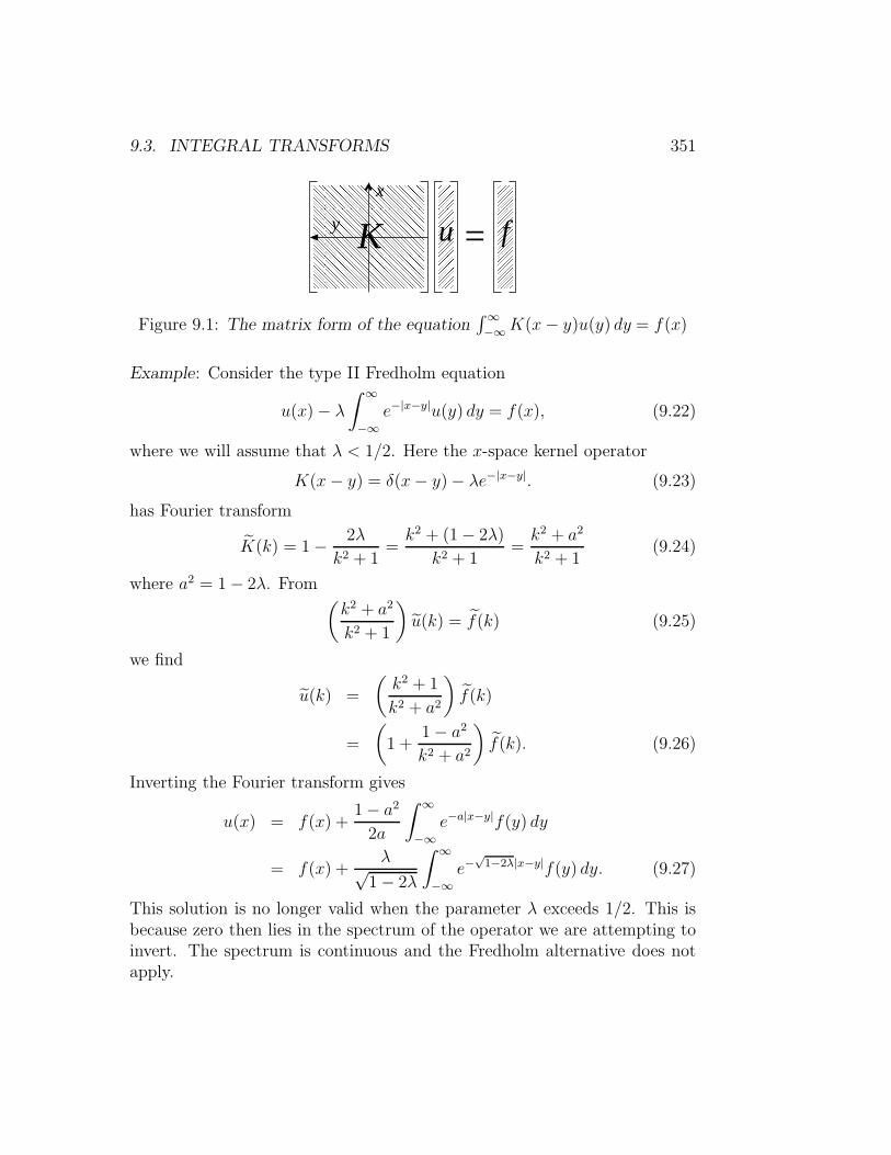
9.3. INTEGRAL TRANSFORMS 351
=u f
x
y K
Figure 9.1: The matrix form of the equation∫∞−∞K(x− y)u(y) dy = f(x)
Example: Consider the type II Fredholm equation
u(x)− λ∫ ∞
−∞e−|x−y|u(y) dy = f(x), (9.22)
where we will assume that λ < 1/2. Here the x-space kernel operator
K(x− y) = δ(x− y)− λe−|x−y|. (9.23)
has Fourier transform
K(k) = 1− 2λ
k2 + 1=k2 + (1− 2λ)
k2 + 1=k2 + a2
k2 + 1(9.24)
where a2 = 1− 2λ. From (k2 + a2
k2 + 1
)u(k) = f(k) (9.25)
we find
u(k) =
(k2 + 1
k2 + a2
)f(k)
=
(1 +
1− a2k2 + a2
)f(k). (9.26)
Inverting the Fourier transform gives
u(x) = f(x) +1− a22a
∫ ∞
−∞e−a|x−y|f(y) dy
= f(x) +λ√
1− 2λ
∫ ∞
−∞e−
√1−2λ|x−y|f(y) dy. (9.27)
This solution is no longer valid when the parameter λ exceeds 1/2. This isbecause zero then lies in the spectrum of the operator we are attempting toinvert. The spectrum is continuous and the Fredholm alternative does notapply.

352 CHAPTER 9. INTEGRAL EQUATIONS
9.3.2 Laplace Transform Methods
The Volterra problem∫ x
0
K(x− y)u(y) dy = f(x), 0 < x <∞. (9.28)
can also be solved by the application of an integral transform. In this casewe observe that value of K(x) is only needed for positive x, and this suggeststhat we take a Laplace transform over the positive real axis.
0 u f0K
0 0 0 0=
x
y
Figure 9.2: We only require the value of K(x) for x positive, and u and fcan be set to zero for x < 0.
Abel’s equation
As an example of Laplace methods, consider Abel’s equation
f(x) =
∫ x
0
1√x− yu(y) dy, (9.29)
where we are given f(x) and wish to find u(x). Here it is clear that we needf(0) = 0 for the equation to make sense. We have met this integral transfor-mation before in the definition of the “half-derivative”. It is an example ofthe more general equation of the form
f(x) =
∫ x
0
K(x− y)u(y) dy. (9.30)
Let us take the Laplace transform of both sides of (9.30):
Lf(p) =
∫ ∞
0
e−px(∫ x
0
K(x− y)u(y) dy)dx
=
∫ ∞
0
dx
∫ x
0
dy e−pxK(x− y)u(y). (9.31)

9.3. INTEGRAL TRANSFORMS 353
Now we make the change of variables
x = ξ + η,
y = η. (9.32)
x
y
x
yx=y
a) b)
ξ=0
dx dξ
Figure 9.3: Regions of integration for the convolution theorem: a) Integratingover y at fixed x, then over x; b) Integrating over η at fixed ξ, then over ξ.
This has Jacobian∂(x, y)
∂(ξ, η)= 1, (9.33)
and the integral becomes
Lf(p) =
∫ ∞
0
∫ ∞
0
e−p(ξ+η)K(ξ)u(η) dξ dη
=
∫ ∞
0
e−pξK(ξ) dξ
∫ ∞
0
e−pηu(η) dη
= LK(p) Lu(p). (9.34)
Thus the Laplace transform of a Volterra convolution is the product of theLaplace transforms. We can now invert
u = L−1(Lf/LK). (9.35)
For Abel’s equation, we have
K(x) =1√x, (9.36)

354 CHAPTER 9. INTEGRAL EQUATIONS
the Laplace transform of which is
LK(p) =
∫ ∞
0
x12−1e−px dx = p−1/2Γ
(1
2
)= p−1/2
√π. (9.37)
Therefore, the Laplace transform of the solution u(x) is
Lu(p) = 1√πp1/2(Lf) = 1
π(√πp−1/2pLf). (9.38)
Now f(0) = 0, and so
pLf = L(d
dxf
), (9.39)
as may be seen by an integration by parts in the definition. Using thisobservation, and depending on whether we put the p next to f or outside theparenthesis, we conclude that the solution of Abel’s equation can be writtenin two equivalent ways:
u(x) =1
π
d
dx
∫ x
0
1√x− yf(y) dy =
1
π
∫ x
0
1√x− yf
′(y) dy. (9.40)
Proving the equality of these two expressions was a problem we set ourselvesin chapter 6.
Here is another way of establishing the equality: Assume for the momentthat K(0) is finite, and that, as we have already noted, f(0) = 0. Then,
d
dx
∫ x
0
K(x− y)f(y) dy (9.41)
is equal to
K(0)f(x) +
∫ x
0
∂xK(x− y)f(y) dy,
= K(0)f(x)−∫ x
0
∂yK(x− y)f(y) dy
= K(0)f(x)−∫ x
0
∂y
(K(x− y)f(y)
)dy +
∫ x
0
K(x− y)f ′(y) dy
= K(0)f(x)−K(0)f(x)−K(x)f(0) +
∫ x
0
K(x− y)f ′(y) dy
=
∫ x
0
K(x− y)f ′(y) dy. (9.42)

9.3. INTEGRAL TRANSFORMS 355
Since K(0) cancelled out, we need not worry that it is divergent! Morerigorously, we should regularize the improper integral by raising the lowerlimit on the integral to a small positive quantity, and then taking the limitto zero at the end of the calculation.
Radon Transforms
detector
patient
X−ray beam
O x
y
θ
t
p
P
Figure 9.4: The geometry of the CAT scan Radon transformation, showingthe location of the point P with co-ordinates x = p cos θ−t sin θ, y = p sin θ+t cos θ.
An Abel integral equation lies at the heart of the method for reconstructingthe image in a computer aided tomography (CAT) scan. By rotating anX-ray source about a patient and recording the direction-dependent shadow,we measure the integral of his tissue density f(x, y) along all lines in a slice(which we will take to be the x, y plane) through his body. The resultinginformation is the Radon transform F of the function f . If we parametrizethe family of lines by p and θ, as shown in figure 9.4, we have
F (p, θ) =
∫ ∞
−∞f(p cos θ − t sin θ, p sin θ + t cos θ) dt,
=
∫
R2
δ(x cos θ + y sin θ − p)f(x, y) dxdy. (9.43)

356 CHAPTER 9. INTEGRAL EQUATIONS
We will assume that f is zero outside some finite region (the patient), andso these integrals converge.
We wish to invert the transformation and recover f from the data F (p, θ).This problem was solved by Johann Radon in 1917. Radon made clever useof the Euclidean group to simplify the problem. He observed that we maytake the point O at which we wish to find f to be the origin, and defined1
FO(p) =1
2π
∫ 2π
0
∫
R2
δ(x cos θ + y sin θ − p) f(x, y) dxdydθ. (9.44)
Thus FO(p) is the angular average over all lines tangent to a circle of ra-dius p about the desired inversion point. Radon then observed that if headditionally defines
f(r) =1
2π
∫ 2π
0
f(r cosφ, r sinφ) dφ (9.45)
then he can substitute f(r) for f(x, y) in (9.44) without changing the valueof the integral. Furthermore f(0) = f(0, 0). Hence, taking polar co-ordinatesin the x, y plane, he has
FO(p) =1
2π
∫ 2π
0
∫
R2
δ(r cosφ cos θ + r sinφ sin θ − p)f(r) rdφdrdθ.
(9.46)We can now use
δ(g(φ)) =∑
n
1
|g′(φn)|δ(φ− φn), (9.47)
where the sum is over the zeros φn of g(φ) = r cos(θ−φ)− p, to perform theφ integral. Any given point x = r cosφ, y = r sinφ lies on two distinct linesif and only if p < r. Thus g(φ) has two zeros if p < r, but none if r < p.Consequently
FO(p) =1
2π
∫ 2π
0
∫ ∞
p
2√r2 − p2
f(r) rdr
dθ. (9.48)
Nothing in the inner integral depends on θ. The outer integral is thereforetrivial, and so
FO(p) =
∫ ∞
p
2√r2 − p2
f(r) rdr. (9.49)
1We trust that the reader will forgive the anachronism of our expressing Radon’s for-mulæ in terms of Dirac’s delta function.

9.3. INTEGRAL TRANSFORMS 357
We can extract FO(p) from the data. We could therefore solve the Abelequation (9.49) and recover the complete function f(r). We are only inter-ested in f(0), however, and it easier verify a claimed solution. Radon assertsthat
f(0, 0) = f(0) = −1
π
∫ ∞
0
1
p
(∂
∂pFO(p)
)dp. (9.50)
To prove that his claim is true we must first take the derivative of FO(p) andshow that (
∂
∂pFO(p)
)=
∫ ∞
p
2p√r2 − p2
(∂
∂rf(r)
)dr. (9.51)
The details of this computation are left as an exercise. It is little differentfrom the differentiation of the integral transform at the end of the last section.We then substitute (9.51) into (9.50) and evaluate the resulting integral
I = −1
π
∫ ∞
0
1
p
∫ ∞
p
2p√r2 − p2
(∂
∂rf(r)
)dr
dp (9.52)
by exchanging the order of the integrations, as shown in figure 9.5.
r
p p=r
r
p p=ra) b)
Figure 9.5: a) In (9.52) we integrate first over r and then over p. The inner rintegral is therefore from r = p to r =∞. b) In (9.53) we integrate first overp and then over r. The inner p integral therefore runs from p = 0 to p = r.
After the interchange we have
I = −2
π
∫ ∞
0
∫ r
0
1√r2 − p2
dp
(∂
∂rf(r)
)dr. (9.53)
Since ∫ r
0
1√r2 − p2
dp =π
2, (9.54)

358 CHAPTER 9. INTEGRAL EQUATIONS
the inner integral is independent of r. We thus obtain
I = −∫ ∞
0
(∂
∂rf(r)
)dr = f(0) = f(0, 0). (9.55)
Radon’s inversion formula is therefore correct.Although Radon found a closed-form inversion formula, the numerical
problem of reconstructing the image from the partial and noisy data obtainedfrom a practical CAT scanner is quite delicate, and remains an active areaof research.
9.4 Separable Kernels
Let
K(x, y) =
N∑
i=1
pi(x)qi(y), (9.56)
where pi and qi are two linearly independent sets of functions. Therange of K is therefore the span 〈pi〉 of the set pi. Such kernels are saidto be separable. The theory of integral equations containing such kernels isespecially transparent.
9.4.1 Eigenvalue problem
Consider the eigenvalue problem
λu(x) =
∫
D
K(x, y)u(y) dy (9.57)
for a separable kernel. Here, D is some range of integration, and x ∈ D. Ifλ 6= 0, we know that u has to be in the range of K, so we can write
u(x) =∑
i
ξipi(x). (9.58)
Inserting this into the integral, we find that our problem reduces to the finitematrix eigenvalue equation
λξi = Aijξj, (9.59)

9.4. SEPARABLE KERNELS 359
where
Aij =
∫
D
qi(y)pj(y) dy. (9.60)
Matters are especially simple when qi = p∗i . In this case Aij = A∗ji, so the
matrix A is Hermitian and has N linearly independent eigenvectors. Further,none of the N associated eigenvalues can be zero. To see that this is sosuppose that v(x) =
∑i ζipi(x) is an eigenvector with zero eigenvalue. In
other words, suppose that
0 =∑
i
pi(x)
∫
D
p∗i (y)pj(y)ζj dy. (9.61)
Since the pi(x) are linearly independent, we must have
0 =
∫
D
p∗i (y)pj(y)ζj dy = 0, (9.62)
for each i separately. Multiplying by ζ∗i and summing we find
0 =
∫
D
∣∣∣∣∣∑
j
pj(y)ζj
∣∣∣∣∣
2
dy =
∫
D
|v(y)|2 dy, (9.63)
and so v(x) itself must have been zero. The remaining (infinite in number)eigenfunctions span 〈qi〉⊥ and have λ = 0.
9.4.2 Inhomogeneous problem
It is easiest to discuss inhomogeneous separable-kernel problems by example.Consider the equation
u(x) = f(x) + µ
∫ 1
0
K(x, y)u(y) dy, (9.64)
where K(x, y) = xy. Here, f(x) and µ are given, and u(x) is to be found.We know that u(x) must be of the form
u(x) = f(x) + ax, (9.65)
and the only task is to find the constant a. We plug u into the integralequation and, after cancelling a common factor of x, we find
a = µ
∫ 1
0
yu(y) dy = µ
∫ 1
0
yf(y) dy+ aµ
∫ 1
0
y2 dy. (9.66)

360 CHAPTER 9. INTEGRAL EQUATIONS
The last integral is equal to µa/3, so
a
(1− 1
3µ
)= µ
∫ 1
0
yf(y) dy, (9.67)
and finally
u(x) = f(x) + xµ
(1 − µ/3)
∫ 1
0
yf(y) dy. (9.68)
Notice that this solution is meaningless if µ = 3. We can relate this to theeigenvalues of the kernel K(x, y) = xy. The eigenvalue problem for thiskernel is
λu(x) =
∫ 1
0
xyu(y) dy. (9.69)
On substituting u(x) = ax, this reduces to λax = ax/3, and so λ = 1/3. Allother eigenvalues are zero. Our inhomogeneous equation was of the form
(1− µK)u = f (9.70)
and the operator (1−µK) has an infinite set of eigenfunctions with eigenvalue1, and a single eigenfunction, u0(x) = x, with eigenvalue (1 − µ/3). Theeigenvalue becomes zero, and hence the inverse ceases to exist, when µ = 3.
A solution to the problem (1−µK)u = f may still exist even when µ = 3.But now, applying the Fredholm alternative, we see that f must satisfy thecondition that it be orthogonal to all solutions of (1− µK)†v = 0. Since ourkernel is Hermitian, this means that f must be orthogonal to the zero modeu0(x) = x. For the case of µ = 3, the equation is
u(x) = f(x) + 3
∫ 1
0
xyu(y) dy, (9.71)
and to have a solution f must obey∫ 1
0yf(y) dy = 0. We again set u =
f(x) + ax, and find
a = 3
∫ 1
0
yf(y) dy + a3
∫ 1
0
y2 dy, (9.72)
but now this reduces to a = a. The general solution is therefore
u = f(x) + ax (9.73)
with a arbitrary.

9.5. SINGULAR INTEGRAL EQUATIONS 361
9.5 Singular Integral Equations
Equations involving principal-part integrals, such as the airfoil equation
P
π
∫ 1
−1
ϕ(x)1
x− y dx = f(y), (9.74)
in which f is given and we are to find ϕ, are called singular integral equations .Their solution depends on what conditions are imposed on the unknownfunction ϕ(x) at the endpoints of the integration region. We will consideronly this simplest example here.2
9.5.1 Solution via Tchebychef Polynomials
Recall the definition of the Tchebychef polynomials from chapter 2. We set
Tn(x) = cos(n cos−1 x), (9.75)
Un−1(x) =sin(n cos−1 x)
sin(cos−1 x)=
1
nT ′n(x). (9.76)
These are the Tchebychef Polynomials of the first and second kind, respec-tively. The orthogonality of the functions cosnθ and sinnθ over the interval[0, π] translates into
∫ 1
−1
1√1− x2
Tn(x) Tm(x) dx = hn δnm, n,m ≥ 0, (9.77)
where h0 = π, hn = π/2, n > 0, and∫ 1
−1
√1− x2 Un−1(x)Um−1(x) dx =
π
2δnm, n,m > 0. (9.78)
The sets Tn(x) and Un(x) are complete in L2w[0, 1] with the weight func-
tions w = (1− x2)−1/2 and w = (1− x2)1/2, respectively .Rather less obvious are the principal-part integral identities (valid for
−1 < y < 1)
P
∫ 1
−1
1√1− x2
1
x− y dx = 0, (9.79)
P
∫ 1
−1
1√1− x2
Tn(x)1
x− y dx = π Un−1(y), n > 0, (9.80)
2The classic text is N. I. Muskhelishvili Singular Integral Equations .

362 CHAPTER 9. INTEGRAL EQUATIONS
and
P
∫ 1
−1
√1− x2 Un−1(x)
1
x− y dx = −π Tn(y), n > 0. (9.81)
These correspond, after we set x = cos θ and y = cos φ, to the trigonometricintegrals
P
∫ π
0
cosnθ
cos θ − cos φdθ = π
sinnφ
sinφ, (9.82)
and
P
∫ π
0
sin θ sinnθ
cos θ − cosφdθ = −π cosnφ, (9.83)
respectively. We will motivate and derive these formulæ at the end of thissection.
Granted the validity of these principal-part integrals we can solve theintegral equation
P
π
∫ 1
−1
ϕ(x)1
x− y dx = f(y), y ∈ [−1, 1], (9.84)
for ϕ in terms of f , subject to the condition that ϕ be bounded at x = ±1.We show that no solution exists unless f satisfies the condition
∫ 1
−1
1√1− x2
f(x) dx = 0, (9.85)
but if f does satisfy this condition then there is a unique solution
ϕ(y) = −√
1− y2π
P
∫ 1
−1
1√1− x2
f(x)1
x− y dx. (9.86)
To understand why this is the solution, and why there is a condition on f ,expand
f(x) =∞∑
n=1
bnTn(x). (9.87)
Here, the condition on f translates into the absence of a term involvingT0 ≡ 1 in the expansion. Then,
ϕ(x) = −√1− x2
∞∑
n=1
bnUn−1(x), (9.88)
9.5. SINGULAR INTEGRAL EQUATIONS 363
with bn the coefficients that appear in the expansion of f , solves the problem.That this is so may be seen on substituting this expansion for ϕ into theintegral equation and using second of the principal-part identities. Thisidentity provides no way to generate a term with T0; hence the constraint.Next we observe that the expansion for ϕ is generated term-by-term fromthe expansion for f by substituting this into the integral form of the solutionand using the first principal-part identity.
Similarly, we solve the for ϕ(y) in
P
π
∫ 1
−1
ϕ(x)1
x− y dx = f(y), y ∈ [−1, 1], (9.89)
where now ϕ is permitted to be singular at x = ±1. In this case there isalways a solution, but it is not unique. The solutions are
ϕ(y) =1
π√
1− y2P
∫ 1
−1
√1− x2f(x) 1
x− y dx+C√1− y2
, (9.90)
where C is an arbitrary constant. To see this, expand
f(x) =
∞∑
n=1
anUn−1(x), (9.91)
and then
ϕ(x) =1√
1− x2
( ∞∑
n=1
anTn(x) + CT0
), (9.92)
satisfies the equation for any value of the constant C. Again the expansionfor ϕ is generated from that of f by use of the second principal-part identity.
Explanation of the Principal-Part Identities
The principal-part identities can be extracted from the analytic properties ofthe resolvent operator Rλ(n − n′) ≡ (H − λI)−1
n,n′ for a tight-binding modelof the conduction band in a one-dimensional crystal with nearest neighbourhopping. The eigenfunctions uE(n) for this problem obey
uE(n+ 1) + uE(n− 1) = E uE(n) (9.93)
and areuE(n) = einθ, −π < θ < π, (9.94)

364 CHAPTER 9. INTEGRAL EQUATIONS
with energy eigenvalues E = 2 cos θ.The resolvent Rλ(n) obeys
Rλ(n+ 1) +Rλ(n− 1)− λRλ(n) = δn0, n ∈ Z, (9.95)
and can be expanded in terms of the energy eigenfunctions as
Rλ(n− n′) =∑
E
uE(n)u∗E(n
′)
E − λ =
∫ π
−π
ei(n−n′)θ
2 cos θ − λdθ
2π(9.96)
If we set λ = 2 cosφ, we observe that
∫ π
−π
einθ
2 cos θ − 2 cosφ
dθ
2π=
1
2i sinφei|n|φ, Im φ > 0. (9.97)
That this integral is correct can be confirmed by observing that it is evalu-ating the Fourier coefficient of the double geometric series
∞∑
n=−∞e−inθei|n|φ =
2i sinφ
2 cos θ − 2 cosφ, Imφ > 0. (9.98)
By writing einθ = cosnθ+i sin nθ and observing that the sine term integratesto zero, we find that
∫ π
0
cosnθ
cos θ − cosφdθ =
π
i sinφ(cosnφ+ i sin nφ), (9.99)
where n > 0, and again we have taken Imφ > 0. Now let φ approach thereal axis from above, and apply the Plemelj formula. We find
P
∫ π
0
cosnθ
cos θ − cos φdθ = π
sinnφ
sinφ. (9.100)
This is the first principal-part integral identity. The second identity,
P
∫ π
0
sin θ sin nθ
cos θ − cosφdθ = −πcosnφ, (9.101)
is obtained from the the first by using the addition theorems for the sine andcosine.
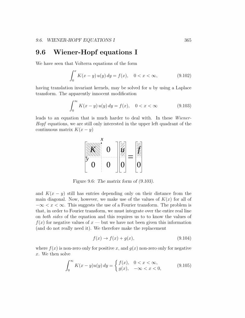
9.6. WIENER-HOPF EQUATIONS I 365
9.6 Wiener-Hopf equations I
We have seen that Volterra equations of the form∫ x
0
K(x− y) u(y) dy = f(x), 0 < x <∞, (9.102)
having translation invariant kernels, may be solved for u by using a Laplacetransform. The apparently innocent modification
∫ ∞
0
K(x− y) u(y) dy = f(x), 0 < x <∞ (9.103)
leads to an equation that is much harder to deal with. In these Wiener-Hopf equations, we are still only interested in the upper left quadrant of thecontinuous matrix K(x− y)
0
0 0 0 0
u fK=
x
y
Figure 9.6: The matrix form of (9.103).
and K(x − y) still has entries depending only on their distance from themain diagonal. Now, however, we make use of the values of K(x) for all of−∞ < x <∞. This suggests the use of a Fourier transform. The problem isthat, in order to Fourier transform, we must integrate over the entire real lineon both sides of the equation and this requires us to to know the values off(x) for negative values of x — but we have not been given this information(and do not really need it). We therefore make the replacement
f(x)→ f(x) + g(x), (9.104)
where f(x) is non-zero only for positive x, and g(x) non-zero only for negativex. We then solve
∫ ∞
0
K(x− y)u(y) dy =f(x), 0 < x <∞,g(x), −∞ < x < 0,
(9.105)

366 CHAPTER 9. INTEGRAL EQUATIONS
so as to find u and g simultaneously. In other words, we extend the problemto one on the whole real line, but with the negative-x source term g(x) chosenso that the solution u(x) is non-zero only for positive x. We represent thispictorially in figure 9.7.
0
u f
g=K
x
y
Figure 9.7: The matrix form of (9.105) with both f and g
To find u and g we try to make an “LU” decomposition of the matrix K intothe product K = L−1U of an upper triangular matrix U(x− y) and a lowertriangular matrix L−1(x− y). Written out in full, the product L−1U is
K(x− y) =∫ ∞
−∞L−1(x− t)U(t − y) dt. (9.106)
Now the inverse of a lower triangular matrix is also lower triangular, and soL(x− y) itself is lower triangular. This means that the function U(x) is zerofor negative x, whilst L(x) is zero when x is positive.
L
U0
0
0
0
0
0
K =
−1x
y
Figure 9.8: The matrix decomposition K = L−1U .
If we can find such a decomposition, then on multiplying both sides by L,equation (9.103) becomes
∫ x
0
U(x− y)u(y) dy = h(x), 0 < x <∞, (9.107)

9.6. WIENER-HOPF EQUATIONS I 367
where
h(x)def=
∫ ∞
x
L(x− y)f(y) dy, 0 < x <∞. (9.108)
These two equations come from the upper half of the full matrix equationrepresented in figure 9.9.
f
L
00
0 g00
0 U=
0
u
0
h
Figure 9.9: The equation (9.107) and the definition (9.108) correspond tothe upper half of these two matrix equations.
The lower parts of the matrix equation have no influence on (9.107) and(9.108): The function h(x) depends only on f , and while g(x) should bechosen to give the column of zeros below h, we do not, in principle, need toknow it. This is because we could solve the Volterra equation Uu = h (9.107)via a Laplace transform. In practice (as we will see) it is easier to find g(x),and then, knowing the (f, g) column vector, obtain u(x) by solving (9.105).This we can do by Fourier transform.
The difficulty lies in finding the LU decomposition. For finite matricesthis decomposition is a standard technique in numerical linear algebra. Itequivalent to the method of Gaussian elimination, which, although we wereprobably never told its name, is the strategy taught in high school for solvingsimultaneous equations. For continuously infinite matrices, however, makingsuch a decomposition demands techniques far beyond those learned in school.It is a particular case of the scalar Riemann-Hilbert problem, and its solutionrequires the use of complex variable methods.
On taking the Fourier transform of (9.106) we see that we are being askedto factorize
K(k) = [L(k)]−1U(k) (9.109)
where
U(k) =
∫ ∞
0
eikxU(x) dx (9.110)

368 CHAPTER 9. INTEGRAL EQUATIONS
is analytic (i.e. has no poles or other singularities) in the region Im k ≥ 0,and similarly
L(k) =
∫ 0
−∞eikxL(x) dx (9.111)
has no poles for Im k ≤ 0, these analyticity conditions being consequencesof the vanishing conditions U(x − y) = 0, x < y and L(x − y) = 0, x > y.
There will be more than one way of factoring K into functions with theseno-pole properties, but, because the inverse of an upper or lower triangu-lar matrix is also upper or lower triangular, the matrices U−1(x − y) andL−1(x − y) have the same vanishing properties, and, because these inversematrices correspond the to the reciprocals of the Fourier transform, we mustalso demand that U(k) and L(k) have no zeros in the upper and lower halfplane respectively. The combined no-poles, no-zeros conditions will usuallydetermine the factors up to constants. If we are able to factorize K(k) in
this manner, we have effected the LU decomposition. When K(k) is a ratio-nal function of k we can factorize by inspection. In the general case, moresophistication is required.
Example: Let us solve the equation
u(x)− λ∫ ∞
0
e−|x−y|u(x) dx = f(x), (9.112)
where we will assume that λ < 1/2. Here the kernel function is
K(x, y) = δ(x− y)− λe−|x−y|. (9.113)
This has Fourier transform
K(k) = 1− 2λ
k2 + 1=k2 + (1− 2λ)
k2 + 1=
(k + ia
k + i
)(k − ik − ia
)−1
. (9.114)
where a2 = 1− 2λ. We were able to factorize this by inspection with
U(k) =k + ia
k + i, L(k) =
k − ik − ia . (9.115)
having poles and zeros only in the lower (respectively upper) half-plane. Wecould now transform back into x space to find U(x− y), L(x− y) and solve
9.6. WIENER-HOPF EQUATIONS I 369
the Volterra equation Uu = h. It is, however, less effort to work directlywith the Fourier transformed equation in the form
(k + ia
k + i
)u+(k) =
(k − ik − ia
)(f+(k) + g−(k)). (9.116)
Here we have placed subscripts on f(k), g(k) and u(k) to remind us that theseFourier transforms are analytic in the upper (+) or lower (-) half-plane. Sincethe left-hand-side of this equation is analytic in the upper half-plane, so mustbe the right-hand-side. We therefore choose g−(k) to eliminate the potentialpole at k = ia that might arise from the first term on the right. This we cando by setting (
k − ik − ia
)g−(k) =
α
k − ia (9.117)
for some as yet undetermined constant α. (Observe that the resultant g−(k)is indeed analytic in the lower half-plane. This analyticity ensures that g(x)is zero for positive x.) We can now solve for u(k) as
u(k) =
(k + i
k + ia
)(k − ik − ia
)f+(k) +
(k + i
k + ia
)α
k − ia
=k2 + 1
k2 + a2f+(k) + α
k + i
k2 + a2
= f+(k) +1− a2k2 + a2
f+(k) + αk + i
k2 + a2(9.118)
The inverse Fourier transform of
k + i
k2 + a2(9.119)
isi
2|a|(1− |a| sgn(x))e−|a||x|, (9.120)
and that of1− a2k2 + a2
=2λ
k2 + (1− 2λ)(9.121)
isλ√
1− 2λe−
√1−2λ|x|. (9.122)

370 CHAPTER 9. INTEGRAL EQUATIONS
Consequently
u(x) = f(x) +λ√
1− 2λ
∫ ∞
0
e−√1−2λ|x−y|f(y) dy
+β(1−√1− 2λ sgn x)e−
√1−2λ|x|. (9.123)
Here β is some multiple of α, and we have used the fact that f(y) is zerofor negative y to make the lower limit on the integral 0 instead of −∞. Wedetermine the as yet unknown β from the requirement that u(x) = 0 forx < 0. We find that this will be the case if we take
β = − λ
a(a + 1)
∫ ∞
0
e−ayf(y) dy. (9.124)
The solution is therefore, for x > 0,
u(x) = f(x) +λ√
1− 2λ
∫ ∞
0
e−√1−2λ|x−y|f(y) dy
+λ(√1− 2λ− 1)
1− 2λ+√1− 2λ
e−√1−2λx
∫ ∞
0
e−√1−2λyf(y) dy. (9.125)
Not every invertible n-by-n matrix has a plain LU decomposition. For arelated reason not every Wiener-Hopf equation can be solved so simply. In-stead there is a topological index theorem that determines whether solutionscan exist, and, if solutions do exist, whether they are unique. We shall there-fore return to this problem once we have aquired a deeper understanding ofthe interaction between topology and complex analysis.
9.7 Some Functional Analysis
We have hitherto avoided, as far as it is possible, the full rigours of mathe-matics. For most of us, and for most of the time, we can solve our physicsproblems by using calculus rather than analysis. It is worth, nonetheless, be-ing familiar with the proper mathematical language so that when somethingtricky comes up we know where to look for help. The modern setting forthe mathematical study of integral and differential equations is the disciplineof functional analysis , and the classic text for the mathematically inclinedphysicist is the four-volume set Methods of Modern Mathematical Physics byMichael Reed and Barry Simon. We cannot summarize these volumes in few
9.7. SOME FUNCTIONAL ANALYSIS 371
paragraphs, but we can try to provide enough background for us to be ableto explain a few issues that may have puzzled the alert reader.
This section requires the reader to have sufficient background in realanalysis to know what it means for a set to be compact.
9.7.1 Bounded and Compact Operators
i) A linear operator K : L2 → L2 is bounded if there is a positive numberM such that
‖Kx‖ ≤M‖x‖, ∀x ∈ L2. (9.126)
If K is bounded then smallest such M is the norm of K, which wedenote by ‖K‖ . Thus
‖Kx‖ ≤ ‖K‖ ‖x‖. (9.127)
For a finite-dimensional matrix, ‖K‖ is the largest eigenvalue of K.The function Kx is a continuous function of x if, and only if, it isbounded. “Bounded” and “continuous” are therefore synonyms. Lineardifferential operators are never bounded, and this is the source of mostof the complications in their theory.
ii) If the operators A and B are bounded, then so is AB and
‖AB‖ ≤ ‖A‖‖B‖. (9.128)
iii) A linear operator K : L2 → L2 is compact (or completely continuous)if it maps bounded sets in L2 to relatively compact sets (sets whoseclosure is compact). Equivalently, K is compact if the image sequenceKxn of every bounded sequence of functions xn contains a convergentsubsequence. Compact ⇒ continuous, but not vice versa. One canshow that, given any positive number M , a compact self-adjoint oper-ator has only a finite number of eigenvalues with λ outside the interval[−M,M ]. The eigenvectors un with non-zero eigenvalues span the rangeof the operator. Any vector can therefore be written
u = u0 +∑
i
aiui, (9.129)
where u0 lies in the null space of K. The Green function of a lineardifferential operator defined on a finite interval is usually the integralkernel of a compact operator.

372 CHAPTER 9. INTEGRAL EQUATIONS
iv) If K is compact thenH = I +K (9.130)
is Fredholm. This means that H has a finite dimensional kernel andco-kernel, and that the Fredholm alternative applies.
v) An integral kernel is Hilbert-Schmidt if∫|K(ξ, η)|2 dξdη <∞. (9.131)
This means thatK can be expanded in terms of a complete orthonormalset φm as
K(x, y) =∞∑
n,m=1
Anmφn(x)φ∗m(y) (9.132)
in the sense that
limN,M→∞
∥∥∥∥∥
N,M∑
n,m=1
Anmφnφ∗m −K
∥∥∥∥∥ = 0. (9.133)
Now the finite sumN,M∑
n,m=1
Anmφn(x)φ∗m(y) (9.134)
is automatically compact since it is bounded and has finite-dimensionalrange. (The unit ball in a Hilbert space is relatively compact ⇔ thespace is finite dimensional). Thus, Hilbert-Schmidt implies that K isapproximated in norm by compact operators. But it is not hard toshow that a norm-convergent limit of compact operators is compact,so K itself is compact. Thus
Hilbert-Schmidt ⇒ compact.
It is easy to test a given kernel to see if it is Hilbert-Schmidt (simplyuse the definition) and therein lies the utility of the concept.
If we have a Hilbert-Schmidt Green function g, we can reacast our differen-tial equation as an integral equation with g as kernel, and this is why theFredholm alternative works for a large class of linear differential equations.Example: Consider the Legendre-equation operator
L = − d
dx(1− x2) d
dx(9.135)

9.7. SOME FUNCTIONAL ANALYSIS 373
acting on functions u ∈ L2[−1, 1] with boundary conditions that u be finiteat the endpoints. This operator has a normalized zero mode u0 = 1/
√2, so
it cannot have an inverse. There exists, however, a modified Green functiong(x, x′) that satisfies
Lu = δ(x− x′)− 1
2. (9.136)
It is
g(x, x′) = ln 2− 1
2− 1
2ln(1 + x>)(1− x<), (9.137)
where x> is the greater of x and x′, and x< the lesser. We may verify that
∫ 1
−1
∫ 1
−1
|g(x, x′)|2 dxdx′ <∞, (9.138)
so g is Hilbert-Schmidt and therefore the kernel of a compact operator. Theeigenvalue problem
Lun = λnun (9.139)
can be recast as as the integral equation
µnun =
∫ 1
−1
g(x, x′)un(x′) dx′ (9.140)
with µn = λ−1n . The compactness of g guarantees that there is a complete
set of eigenfunctions (these being the Legendre polynomials Pn(x) for n > 0)having eigenvalues µn = 1/n(n+1). The operator g also has the eigenfunctionP0 with eigenvalue µ0 = 0. This example provides the justification for theclaim that the “finite” boundary conditions we adopted for the Legendreequation in chapter 8 give us a self adjoint operator.
Note that K(x, y) does not have to be bounded for K to be Hilbert-Schmidt.Example: The kernel
K(x, y) =1
(x− y)α , |x|, |y| < 1 (9.141)
is Hilbert-Schmidt provided α < 12.
Example: The kernel
K(x, y) =1
2me−m|x−y|, x, y ∈ R (9.142)

374 CHAPTER 9. INTEGRAL EQUATIONS
is not Hilbert-Schmidt because |K(x − y)| is constant along the the linesx − y = constant, which lie parallel to the diagonal. K has a continuousspectrum consisting of all positive real numbers less than 1/m2. It cannotbe compact, therefore, but it is bounded with ‖K‖ = 1/m2. The integralequation (9.22) contains this kernel, and the Fredholm alternative does notapply to it.
9.7.2 Closed Operators
One motivation for our including a brief account of functional analysis isthat an attentive reader will have realized that some of the statements wehave made in earlier chapters appear to be inconsistent. We have asserted inchapter 2 that no significance can be attached to the value of an L2 functionat any particular point — only integrated averages matter. In later chapters,though, we have happily imposed boundary conditions that require thesevery functions to take specified values at the endpoints of our interval. In thissection we will resolve this paradox. The apparent contradiction is intimatelyconnected with our imposing boundary conditions only on derivatives of lowerorder than than that of the differential equation, but understanding why thisis so requires some function-analytic language.
Differential operators L are never continuous; we cannot deduce fromun → u that Lun → Lu. Differential operators can be closed , however. Aclosed operator is one for which whenever a sequence un converges to a limitu and at the same time the image sequence Lun also converges to a limit f ,then u is in the domain of L and Lu = f . The name is not meant to implythat the domain of definition is closed, but indicates instead that the graphof L — this being the set u, Lu considered as a subset of L2[a, b]×L2[a, b]— contains its limit points and so is a closed set.
Any self-adjoint operator is automatically closed. To see why this is so,recall that in the defining the adjoint of an operator A, we say that y is in thedomain of A† if there is a z such that 〈y, Ax〉 = 〈z, x〉 for all x in the domainof A. We then set A†y = z. Now suppose that yn → y and A†yn = zn → z.The Cauchy-Schwartz-Bunyakovski inequality shows that the inner productis a continuous function of its arguments. Consequently, if x is in the domainof A, we can take the limit of 〈yn, Ax〉 = 〈A†yn, x〉 = 〈zn, x〉 to deduce that〈y, Ax〉 = 〈z, x〉. But this means that y is in the domain of A†, and z = A†y.The adjoint of any operator is therefore a closed operator. A self-adjointoperator, being its own adjoint, is therefore necessarily closed.

9.7. SOME FUNCTIONAL ANALYSIS 375
A deep result states that a closed operator defined on a closed domain isbounded. Since they are always unbounded, the domain of a closed differen-tial operator can never be a closed set.
An operator may not be closed but may be closable, in that we canmake it closed by including additional functions in its domain. The essentialrequirement for closability is that we never have two sequences un and vnwhich converge to the same limit, w, while Lun and Lvn both converge, butto different limits. Closability is equivalent to requiring that if un → 0 andLun converges, then Lun converges to zero.
Example: Let L = d/dx. Suppose that un → 0 and Lun → f . If ϕ is asmooth L2 function that vanishes at 0, 1, then
∫ 1
0
ϕf dx = limn→∞
∫ 1
0
ϕdundx
dx = − limn→∞
∫ 1
0
φ′un dx = 0. (9.143)
Here we have used the continuity of the inner product to justify the inter-change the order of limit and integral. By the same arguments we used whendealing with the calculus of variations, we deduce that f = 0. Thus d/dx isclosable.
If an operator is closable, we may as well add the extra functions to itsdomain and make it closed. Let us consider what closure means for theoperator
L =d
dx, D(L) = y ∈ C1[0, 1] : y′(0) = 0. (9.144)
Here, in fixing the derivative at the endpoint, we are imposing a boundarycondition of higher order than we ought.
Consider the sequence of differentiable functions ya shown in figure 9.10.These functions have vanishing derivative at x = 0, but tend in L2 to afunction y whose derivative is non-zero at x = 0.

376 CHAPTER 9. INTEGRAL EQUATIONS
a
yay
Figure 9.10: lima→0 ya = y in L2[0, 1] .
Figure 9.11 shows that derivative of these functions also converges in L2.
a
ay’ y’
Figure 9.11: y′a → y′ in L2[0, 1] .
If we want L to be closed, we should therefore extend the domain of definitionof L to include functions with non-vanishing endpoint derivative. We can alsouse this method to add to the domain of L functions that are only piecewisedifferentiable — i.e. functions with a discontinuous derivative.
Now consider what happens if we try to extend the domain of
L =d
dx, D(L) = y, y′ ∈ L2 : y(0) = 0, (9.145)
to include functions that do not vanish at the endpoint. Take a sequence thesequence of functions ya shown in figure 9.12. These functions vanish at theorigin, and converge in L2 to a function that does not vanish at the origin.

9.7. SOME FUNCTIONAL ANALYSIS 377
a
yay
1 1
Figure 9.12: lima→0 ya = y in L2[0, 1].
Now, as figure 9.13 shows, the derivatives converge towards the derivativeof the limit function — together with a delta function near the origin. Thearea under the functions |y′a(x)|2 grows without bound and the sequence Lyabecomes infinitely far from the derivative of the limit function when distanceis measured in the L2 norm.
a
a
1/a
y’
δ(x)
Figure 9.13: y′a → δ(x), but the delta function is not an element of L2[0, 1] .
We therefore cannot use closure to extend the domain to include these func-tions. Another way of saying this is, that in order for the weak derivative ofy to be in L2, and therefore for y to be in the domain of d/dx, the function yneed not be classically differentiable, but its L2 equivalence class must con-tain a continuous function — and continuous functions do have well-definedvalues. It is the values of this continuous representative that are constrainedby the boundary conditions.
This story repeats for differential operators of any order: If we try toimpose boundary conditions of too high an order, they are washed out in the

378 CHAPTER 9. INTEGRAL EQUATIONS
process of closing the operator. Boundary conditions of lower order cannotbe eliminated, however, and so make sense as statements involving functionsin L2.
9.8 Series Solutions
One of the advantages of recasting a problem as an integral equation, is thatthe equation often suggests a systematic approximation scheme. Usually westart from the solution of an exactly solvable problem and expand the desiredsolution about it as an infinite series in some small parameter. The terms insuch a perturbation series may become progressively harder to evaluate, but,if we are lucky, the sum of the first few will prove adaquate for our purposes.
9.8.1 Liouville-Neumann-Born Series
The geometric seriesS = 1− x+ x2 − x3 + · · · (9.146)
converges to 1/(1 + x) provided |x| < 1. Suppose we wish to solve
(I + λK)ϕ = f (9.147)
where K is a an integral operator. It is then natural to write
ϕ = (I + λK)−1f = (1− λK + λ2K2 − λ3K3 + · · ·)f (9.148)
where
K2(x, y) =
∫K(x, z)K(z, y) dz, K3(x, y) =
∫K(x, z1)K(z1, z2)K(z2, y) dz1dz2,
(9.149)and so on. This Liouville-Neumann series will converge, and yield a solutionto the problem, provided that λ‖K‖ < 1. In quantum mechanics this seriesis known as the Born series .
9.8.2 Fredholm Series
A familiar result from high-school algebra is Cramer’s rule, which gives thesolution of a set of linear equations in terms of ratios of determinants. For

9.8. SERIES SOLUTIONS 379
example, the system of equations
a11x1 + a12x2 + a13x3 = b1,
a21x1 + a22x2 + a23x3 = b2,
a31x1 + a32x2 + a33x3 = b3, (9.150)
has solution
x1 =1
D
∣∣∣∣∣∣
b1 a12 a13b2 a22 a23b3 a32 a33
∣∣∣∣∣∣, x2 =
1
D
∣∣∣∣∣∣
a11 b1 a13a21 b2 a23a31 b3 a33
∣∣∣∣∣∣, x3 =
1
D
∣∣∣∣∣∣
a11 a12 b1a21 a22 b2a31 a32 b3
∣∣∣∣∣∣,
(9.151)where
D =
∣∣∣∣∣∣
a11 a12 a13a21 a22 a23a31 a32 a33
∣∣∣∣∣∣. (9.152)
Although not as computationally efficient as standard Gaussian elimination,Cramer’s rule is useful in that it is a closed-form solution. It is equivalent tothe statement that the inverse of a matrix is given by the transposed matrixof the co-factors, divided by the determinant.
A similar formula for integral equations was given by Fredholm. Theequations he considered were, in operator form
(I + λK)ϕ = f. (9.153)
Where I is the identity operator, K is an integral operator with kernelK(x, y), and λ a parameter We motivate Fredholm’s formula by giving anexpansion for the determinant of a finite matrix. Let K be an n-by-n matrix
D(λ)def= det (I+ λK) ≡
∣∣∣∣∣∣∣∣
1 + λK11 λK12 · · · λK1n
λK21 1 + λK22 · · · λK2n...
.... . .
...λKn1 λKn2 · · · 1 + λKnn
∣∣∣∣∣∣∣∣. (9.154)
Then
D(λ) =
n∑
m=0
λm
m!Am, (9.155)
where A0 = 1, A1 = trK ≡∑iKii,
A2 =
n∑
i1,i2=1
∣∣∣∣Ki1i1 Ki1i2
Ki2i1 Ki2i2
∣∣∣∣ , A3 =
n∑
i1,i2,i3=1
∣∣∣∣∣∣
Ki1i1 Ki1i2 Ki1i3
Ki2i1 Ki2i2 Ki2i3
Ki3i1 Ki3i2 Ki3i3
∣∣∣∣∣∣. (9.156)

380 CHAPTER 9. INTEGRAL EQUATIONS
The pattern for the rest of the terms should be obvious, as should the proof.As observed above, the inverse of a matrix is the reciprocal of the deter-
minant of the matrix multiplied by the transposed matrix of the co-factors.So, if Dµν is the co-factor of the term in D(λ) associated with Kνµ, then thesolution of the matrix equation
(I+ λK)x = b (9.157)
is
xµ =Dµ1b1 +Dµ2b2 + · · ·+Dµnbn
D(λ). (9.158)
If µ 6= ν we have
Dµν = λKµν + λ2∑
i
∣∣∣∣Kµν Kµi
Kiν Kii
∣∣∣∣+ λ31
2!
∑
i1i2
∣∣∣∣∣∣
Kµν Kµi1 Kµi2
Ki1ν Ki1i1 Ki1i2
Ki2ν Ki2i1 Ki2i2
∣∣∣∣∣∣+ · · · .
(9.159)When µ = ν we have
Dµν = δµνD(λ) (9.160)
where D(λ) is the expression analogous to D(λ), but with the µ’th row andcolumn deleted.
These elementary results suggest the definition of the Fredholm determi-nant of the integral kernel K(x, y), a < x, y < b, as
D(λ) = Det |I + λK| ≡∞∑
m=0
λm
m!Am, (9.161)
where A0 = 1, A1 = TrK ≡∫ baK(x, x) dx,
A2 =
∫ b
a
∫ b
a
∣∣∣∣K(x1, x1) K(x1, x2)K(x2, x1) K(x2, x2)
∣∣∣∣ dx1dx2,
A3 =
∫ b
a
∫ b
a
∫ b
a
∣∣∣∣∣∣
K(x1, x1) K(x1, x2) K(x1, x3)K(x2, x1) K(x2, x2) K(x2, x3)K(x3, x1) K(x3, x2) K(x3, x3)
∣∣∣∣∣∣dx1dx2dx3. (9.162)
etc. We also define
D(x, y, λ) = λK(x, y) + λ2∫ b
a
∣∣∣∣K(x, y) K(x, ξ)K(ξ, y) K(ξ, ξ)
∣∣∣∣ dξ

9.8. SERIES SOLUTIONS 381
+λ31
2!
∫ b
a
∫ b
a
∣∣∣∣∣∣
K(x, y) K(x, ξ1) K(x, ξ2)K(ξ1, y) K(ξ1, ξ1) K(ξ1, ξ2)K(ξ2, y) K(ξ2, ξ1) K(ξ2, ξ2)
∣∣∣∣∣∣dξ1dξ2 + · · · ,
(9.163)
and then
ϕ(x) = f(x) +1
D(λ)
∫ b
a
D(x, y, λ)f(y) dy (9.164)
is the solution of the equation
ϕ(x) + λ
∫ b
a
K(x, y)ϕ(y) dy = f(x). (9.165)
If |K(x, y)| < M in [a, b]× [a, b], the Fredholm series for D(λ) and D(x, y, λ)converge for all λ, and define entire functions. In this feature it is unlike theNeumann series, which has a finite radius of convergence.
The proof of these claims follows from the identity
D(x, y, λ) + λD(λ)K(x, y) + λ
∫ b
a
D(x, ξ, λ)K(ξ, y) dξ = 0, (9.166)
or, more compactly with G(x, y) = D(x, y, λ)/D(λ),
(I +G)(I + λK) = I. (9.167)
For details see Whitaker and Watson §11.2.Example: The equation
ϕ(x) = x+ λ
∫ 1
0
xyϕ(y) dy (9.168)
gives us
D(λ) = 1− 1
3λ, D(x, y, λ) = λxy (9.169)
and so
ϕ(x) =3x
3− λ. (9.170)
(We have considered this equation and solution before, in section 9.4 )

382 CHAPTER 9. INTEGRAL EQUATIONS
9.9 Further Exercises and Problems
Exercise 9.1: The following problems should be relatively easy.
a) Solve the inhomogeneous type II Fredholm integral equation
u(x) = ex + λ
∫ 1
0xy u(y) dy .
b) Solve the homogeneous type II Fredholm integral equation
u(x) = λ
∫ π
0sin(x− y)u(y) dy .
c) Solve the integral equation
u(x) = x+ λ
∫ 1
0(yx+ y2)u(y) dy
to second order in λ using(i) the Neumann series; and(ii) the Fredholm series.
d) By differentiating, solve the integral equation: u(x) = x+∫ x0 u(y) dy.
e) Solve the integral equation: u(x) = x2 +∫ 10 xy u(y) dy.
f) Find the eigenfunction(s) and eigenvalue(s) of the integral equation
u(x) = λ
∫ 1
0ex−y u(y) dy .
g) Solve the integral equation: u(x) = ex + λ∫ 10 ex−y u(y) dy.
h) Solve the integral equation
u(x) = x+
∫ 1
0dy (1 + xy)u(y)
for the unknown function u(x).
Exercise 9.2: Solve the integral equation
u(x) = f(x) + λ
∫ 1
0x3y3u(y)dy, 0 < x < 1
for the unknown u(x) in terms of the given function f(x). For what valuesof λ does a unique solution u(x) exist without restrictions on f(x)? For what

9.9. FURTHER EXERCISES AND PROBLEMS 383
value λ = λ0 does a solution exist only if f(x) satisfies some condition? Usingthe language of the Fredholm alternative, and the range and nullspace of therelevant operators, explain what is happening when λ = λ0. For the caseλ = λ0 find explicitly the condition on f(x) and, assuming this condition issatisfied, write down the corresponding general solution for u(x). Check thatthis solution does indeed satisfy the integral equation.
Exercise 9.3: Use a Laplace transform to find the solution to the generalizedAbel equation
f(x) =
∫ x
0(x− t)−µ u(t)dt, 0 < µ < 1,
where f(x) is given and f(0) = 0. Your solution will be of the form
u(x) =
∫ x
0K(x− t)f ′(t)dt,
and you should give an explicit expression for the kernel K(x− t).You will find the formula
∫ ∞
0tµ−1e−ptdt = p−µ Γ(µ), µ > 0.
to be useful.
Exercise 9.4: Translationally invariant kernels:
a) Consider the integral equation: u(x) = g(x) + λ∫∞−∞K(x, y)u(y) dy,
with the translationally invariant kernel K(x, y) = Q(x− y), in which g,λ and Q are known. Show that the Fourier transforms u, g and Q satisfyu(q) = g(q)/1 −
√2πλQ(q). Expand this result to second order in λ
to recover the second-order Liouville-Neumann-Born series.b) Use Fourier transforms to find a solution of the integral equation
u(x) = e−|x| + λ
∫ ∞
−∞e−|x−y| u(y) dy
that remains finite as |x| → ∞.c) Use Laplace transforms to find a solution of the integral equation
u(x) = e−x + λ
∫ x
0e−|x−y| u(y) dy x > 0.

384 CHAPTER 9. INTEGRAL EQUATIONS
Exercise 9.5: The integral equation
1
π
∫ ∞
0dy
φ(y)
x+ y= f(x), x > 0,
relates the unknown function φ to the known function f .
(i) Show that the changes of variables
x = exp 2ξ, y = exp 2η, φ(exp 2η) exp η = ψ(η), f(exp 2ξ) exp ξ = g(ξ),
converts the integral equation into one that can be solved by an integraltransform.
(ii) Hence, or otherwise, construct an explicit formula for φ(x) in terms of adouble integral involving f(y).
You may use without proof the integral∫ ∞
−∞dξ
e−isξ
cosh ξ=
π
cosh πs/2.
Exercise 9.6: Using Mellin transforms. Recall that the Mellin transform f(s)of the function f(t) is defined by
f(s) =
∫ ∞
0dt ts−1 f(t) .
a) Given two functions, f(t) and g(t), a Mellin convolution f ∗ g can bedefined through
(f ∗ g)(t) =∫ ∞
0f(tu−1) g(u)
du
u
Show that the Mellin transform of the Mellin convolution f ∗ g is
f ∗ g(s) =∫ ∞
0ts−1(f ∗ g)(t) dt = f(s)g(s).
Similarly find the Mellin transform of
(f#g)(t)def=
∫ ∞
0f(tu)g(u) du.
b) The unknown function F (t) satisfies Fox’s integral equation,
F (t) = G(t) +
∫ ∞
0dv Q(tv)F (v),
in which G and Q are known. Solve for the Mellin transform F in termsof the Mellin transforms G and Q.

9.9. FURTHER EXERCISES AND PROBLEMS 385
Exercise 9.7: Some more easy problems:
a) Solve the Lalesco-Picard integral equation
u(x) = cosµx+
∫ ∞
−∞dy e−|x−y| u(y) .
b) For λ 6= 3, solve the integral equation
φ(x) = 1 + λ
∫ 1
0dy xy φ(y) .
c) By taking derivatives, show that the solution of the Volterra equation
x =
∫ x
0dy (ex + ey)ψ(y)
satisfies a first order differential equation. Hence, solve the integral equa-tion.
Exercise 9.8: Principal part integrals.
a) If w is real, show that
P
∫ ∞
−∞e−u
2 1
u− wdu = −2√πe−w2
∫ w
0eu
2
du.
(This is easier than it looks.)b) If y is real, but not in the interval (−1, 1), show that
∫ 1
−1
1
(y − x)√1− x2
dx =π√y2 − 1
.
Now let y ∈ (−1, 1). Show that
P
∫ 1
−1
1
(y − x)√1− x2
dx = 0.
(This is harder than it looks.)
Exercise 9.9:
Consider the integral equation
u(x) = g(x) + λ
∫ 1
0K(x, y)u(y) dy ,
in which only u is unknown.

386 CHAPTER 9. INTEGRAL EQUATIONS
a) Write down the solution u(x) to second order in the Liouville-Neumann-Born series.
b) Suppose g(x) = x and K(x, y) = sin 2πxy. Compute u(x) to secondorder in the Liouville-Neumann-Born series.
Exercise 9.10:: Show that the application of the Fredholm series method tothe equation
ϕ(x) = x+ λ
∫ 1
0(xy + y2)ϕ(y) dy
gives
D(λ) = 1− 2
3λ− 1
72λ2
and
D(x, y, λ) = λ(xy + y2) + λ2(1
2xy2 − 1
3xy − 1
3y2 +
1
4y).

Chapter 10
Vectors and Tensors
In this chapter we explain how a vector space V gives rise to a family ofassociated tensor spaces, and how mathematical objects such as linear mapsor quadratic forms should be understood as being elements of these spaces.We then apply these ideas to physics. We make extensive use of notions andnotations from the appendix on linear algebra, so it may help to review thatmaterial before we begin.
10.1 Covariant and Contravariant Vectors
When we have a vector space V over R, and e1, e2, . . . , en and e′1, e′2, . . . , e′nare both bases for V , then we may expand each of the basis vectors eµ interms of the e′µ as
eν = aµνe′µ. (10.1)
We are here, as usual, using the Einstein summation convention that repeatedindices are to be summed over. Written out in full for a three-dimensionalspace, the expansion would be
e1 = a11e′1 + a21e
′2 + a31e
′3,
e2 = a12e′1 + a22e
′2 + a32e
′3,
e3 = a13e′1 + a23e
′2 + a33e
′3.
We could also have expanded the e′µ in terms of the eµ as
e′ν = (a−1)µνeµ. (10.2)
387

388 CHAPTER 10. VECTORS AND TENSORS
As the notation implies, the matrices of coefficients aµν and (a−1)µν are inversesof each other:
aµν (a−1)νσ = (a−1)µνa
νσ = δµσ . (10.3)
If we know the components xµ of a vector x in the eµ basis then the compo-nents x′µ of x in the e′µ basis are obtained from
x = x′µe′µ = xνeν = (xνaµν ) e′µ (10.4)
by comparing the coefficients of e′µ. We find that x′µ = aµνxν . Observe how
the eµ and the xµ transform in “opposite” directions. The components xµ
are therefore said to transform contravariantly .Associated with the vector space V is its dual space V ∗, whose elements
are covectors , i.e. linear maps f : V → R. If f ∈ V ∗ and x = xµeµ, we usethe linearity property to evaluate f(x) as
f(x) = f(xµeµ) = xµf(eµ) = xµ fµ. (10.5)
Here, the set of numbers fµ = f(eµ) are the components of the covector f . Ifwe change basis so that eν = aµνe
′µ then
fν = f(eν) = f(aµνe′µ) = aµν f(e
′µ) = aµνf
′µ. (10.6)
We conclude that fν = aµνf′µ. The fµ components transform in the same man-
ner as the basis. They are therefore said to transform covariantly . In physicsit is traditional to call the the set of numbers xµ with upstairs indices (thecomponents of) a contravariant vector . Similarly, the set of numbers fµ withdownstairs indices is called (the components of) a covariant vector . Thus,contravariant vectors are elements of V and covariant vectors are elementsof V ∗.
The relationship between V and V ∗ is one of mutual duality, and tomathematicians it is only a matter of convenience which space is V andwhich space is V ∗. The evaluation of f ∈ V ∗ on x ∈ V is therefore oftenwritten as a “pairing” (f ,x), which gives equal status to the objects beingput togther to get a number. A physics example of such a mutually dual pairis provided by the space of displacements x and the space of wave-numbersk. The units of x and k are different (meters versus meters−1). There istherefore no meaning to “x+ k,” and x and k are not elements of the samevector space. The “dot” in expressions such as
ψ(x) = eik·x (10.7)
10.1. COVARIANT AND CONTRAVARIANT VECTORS 389
cannot be a true inner product (which requires the objects it links to be inthe same vector space) but is instead a pairing
(k,x) ≡ k(x) = kµxµ. (10.8)
In describing the physical world we usually give priority to the space in whichwe live, breathe and move, and so treat it as being “V ”. The displacementvector x then becomes the contravariant vector, and the Fourier-space wave-number k, being the more abstract quantity, becomes the covariant covector.
Our vector space may come equipped with a metric that is derived froma non-degenerate inner product. We regard the inner product as being abilinear form g : V × V → R, so the length ‖x‖ of a vector x is
√g(x,x).
The set of numbersgµν = g(eµ, eν) (10.9)
comprises the (components of) the metric tensor . In terms of them, theinner of product 〈x,y〉 of pair of vectors x = xµeµ and y = yµeµ becomes
〈x,y〉 ≡ g(x,y) = gµνxµyν. (10.10)
Real-valued inner products are always symmetric, so g(x,y) = g(y,x) andgµν = gνµ. As the product is non-degenerate, the matrix gµν has an inverse,which is traditionally written as gµν . Thus
gµνgνλ = gλνgνµ = δλµ. (10.11)
The additional structure provided by the metric permits us to identify Vwith V ∗. The identification is possible, because, given any f ∈ V ∗, we canfind a vector f ∈ V such that
f(x) = 〈f ,x〉. (10.12)
We obtain f by solving the equation
fµ = gµν fν (10.13)
to get f ν = gνµfµ. We may now drop the tilde and identify f with f , andhence V with V ∗. When we do this, we say that the covariant componentsfµ are related to the contravariant components fµ by raising
fµ = gµνfν , (10.14)

390 CHAPTER 10. VECTORS AND TENSORS
or lowering
fµ = gµνfν , (10.15)
the index µ using the metric tensor. Bear in mind that this V ∼= V ∗ identi-fication depends crucially on the metric. A different metric will, in general,identify an f ∈ V ∗ with a completely different f ∈ V .
We may play this game in the Euclidean space En with its “dot” innerproduct. Given a vector x and a basis eµ for which gµν = eµ · eν , we candefine two sets of components for the same vector. Firstly the coefficients xµ
appearing in the basis expansion
x = xµeµ, (10.16)
and secondly the “components”
xµ = eµ · x = g(eµ,x) = g(eµ, xνeν) = g(eµ, eν)x
ν = gµνxν (10.17)
of x along the basis vectors. These two set of numbers are then respectivelycalled the contravariant and covariant components of the vector x. If theeµ constitute an orthonormal basis, where gµν = δµν , then the two sets ofcomponents (covariant and contravariant) are numerically coincident. In anon-orthogonal basis they will be different, and we must take care never toadd contravariant components to covariant ones.
10.2 Tensors
We now introduce tensors in two ways: firstly as sets of numbers labelled byindices and equipped with transformation laws that tell us how these numberschange as we change basis; and secondly as basis-independent objects thatare elements of a vector space constructed by taking multiple tensor productsof the spaces V and V ∗.
10.2.1 Transformation rules
After we change basis eµ → e′µ, where eν = aµνe′µ, the metric tensor will be
represented by a new set of components
g′µν = g(e′µ, e′ν). (10.18)

10.2. TENSORS 391
These are be related to the old components by
gµν = g(eµ, eν) = g(aρµe′ρ, a
σνe
′σ) = aρµa
σνg(e
′ρ, e
′σ) = aρµa
σν g
′ρσ. (10.19)
This transformation rule for gµν has both of its subscripts behaving like thedownstairs indices of a covector. We therefore say that gµν transforms as adoubly covariant tensor . Written out in full, for a two-dimensional space,the transformation law is
g11 = a11a11g
′11 + a11a
21g
′12 + a21a
11g
′21 + a21a
21g
′22,
g12 = a11a12g
′11 + a11a
22g
′12 + a21a
12g
′21 + a21a
22g
′22,
g21 = a12a11g
′11 + a12a
21g
′12 + a22a
11g
′21 + a22a
21g
′22,
g22 = a12a12g
′11 + a12a
22g
′12 + a22a
12g
′21 + a22a
22g
′22.
In three dimensions each row would have nine terms, and sixteen in fourdimensions.
A set of numbers Qαβγδǫ, whose indices range from 1 to the dimension of
the space and that transforms as
Qαβγδǫ = (a−1)αα′(a−1)ββ′ a
γ′
γ aδ′
δ aǫ′
ǫ Q′α′β′
γ′δ′ǫ′, (10.20)
or conversely as
Q′αβγδǫ = aαα′a
ββ′(a
−1)γ′
γ (a−1)δ
′
δ (a−1)ǫ
′
ǫ Qα′β′
γ′δ′ǫ′, (10.21)
comprises the components of a doubly contravariant, triply covariant tensor.More compactly, the Qαβ
γδǫ are the components of a tensor of type (2, 3).Tensors of type (p, q) are defined analogously. The total number of indicesp+ q is called the rank of the tensor.
Note how the indices are wired up in the transformation rules (10.20)and (10.21): free (not summed over) upstairs indices on the left hand sideof the equations match to free upstairs indices on the right hand side, simi-larly for the downstairs indices. Also upstairs indices are summed only withdownstairs ones.
Similar conditions apply to equations relating tensors in any particularbasis. If they are violated you do not have a valid tensor equation — meaningthat an equation valid in one basis will not be valid in another basis. Thusan equation
Aµνλ = Bµτνλτ + Cµ
νλ (10.22)

392 CHAPTER 10. VECTORS AND TENSORS
is fine, but
Aµνλ?= Bν
µλ + Cµνλσσ +Dµ
νλτ (10.23)
has something wrong in each term.Incidentally, although not illegal, it is a good idea not to write tensor
indices directly underneath one another — i.e. do not write Qijkjl — because
if you raise or lower indices using the metric tensor, and some pages later ina calculation try to put them back where they were, they might end up inthe wrong order.
Tensor algebra
The sum of two tensors of a given type is also a tensor of that type. The sumof two tensors of different types is not a tensor. Thus each particular type oftensor constitutes a distinct vector space, but one derived from the commonunderlying vector space whose change-of-basis formula is being utilized.
Tensors can be combined by multiplication: if Aµνλ and Bµνλτ are tensors
of type (1, 2) and (1, 3) respectively, then
Cαβνλρστ = AανλB
βρστ (10.24)
is a tensor of type (2, 5).An important operation is contraction, which consists of setting one or
more contravariant index index equal to a covariant index and summing overthe repeated indices. This reduces the rank of the tensor. So, for example,
Dρστ = Cαβαβρστ (10.25)
is a tensor of type (0, 3). Similarly f(x) = fµxµ is a type (0, 0) tensor, i.e. an
invariant — a number that takes the same value in all bases. Upper indicescan only be contracted with lower indices, and vice versa. For example, thearray of numbers Aα = Bαββ obtained from the type (0, 3) tensor Bαβγ is nota tensor of type (0, 1).
The contraction procedure outputs a tensor because setting an upperindex and a lower index to a common value µ and summing over µ, leads tothe factor . . . (a−1)µαa
βµ . . . appearing in the transformation rule. Now
(a−1)µαaβµ = δβα, (10.26)
and the Kronecker delta effects a summation over the corresponding pair ofindices in the transformed tensor.

10.2. TENSORS 393
Although often associated with general relativity, tensors occur in manyplaces in physics. They are used, for example, in elasticity theory, where theword “tensor” in its modern meaning was introduced by Woldemar Voigtin 1898. Voigt, following Cauchy and Green, described the infinitesimaldeformation of an elastic body by the strain tensor eαβ , which is a tensorof type (0,2). The forces to which the strain gives rise are described by thestress tensor σλµ. A generalization of Hooke’s law relates stress to strain viaa tensor of elastic constants cαβγδ as
σαβ = cαβγδeγδ. (10.27)
We study stress and strain in more detail later in this chapter.
Exercise 10.1: Show that gµν , the matrix inverse of the metric tensor gµν , isindeed a doubly contravariant tensor, as the position of its indices suggests.
10.2.2 Tensor character of linear maps and quadratic
forms
As an illustration of the tensor concept and of the need to distinguish be-tween upstairs and downstairs indices, we contrast the properties of matricesrepresenting linear maps and those representing quadratic forms.
A linear map M : V → V is an object that exists independently of anybasis. Given a basis, however, it is represented by a matrix Mµ
ν obtainedby examining the action of the map on the basis elements:
M(eµ) = eνMνµ. (10.28)
Acting on x we get a new vector y =M(x), where
yνeν = y =M(x) =M(xµeµ) = xµM(eµ) = xµMνµeν =Mν
µxµ eν . (10.29)
We therefore haveyν =Mν
µxµ, (10.30)
which is the usual matrix multiplication y = Mx. When we change basis,eν = aµνe
′µ, then
eνMνµ =M(eµ) =M(aρµe
′ρ) = aρµM(e′ρ) = aρµe
′σM
′σρ = aρµ(a
−1)νσeνM′σρ.
(10.31)

394 CHAPTER 10. VECTORS AND TENSORS
Comparing coefficients of eν , we find
Mνµ = aρµ(a
−1)νσM′σρ, (10.32)
or, conversely,M ′ν
µ = (a−1)ρµaνσM
σρ. (10.33)
Thus a matrix representing a linear map has the tensor character suggestedby the position of its indices, i.e. it transforms as a type (1, 1) tensor. We canderive the same formula in matrix notation. In the new basis the vectors xand y have new components x′ = Ax, and y′ = Ay. Consequently y = Mxbecomes
y′ = Ay = AMx = AMA−1x′, (10.34)
and the matrix representing the map M has new components
M′ = AMA−1. (10.35)
Now consider the quadratic form Q : V → R that is obtained from asymmetric bilinear form Q : V × V → R by setting Q(x) = Q(x,x). We canwrite
Q(x) = Qµνxµxν = xµQµν x
ν = xTQx, (10.36)
where Qµν ≡ Q(eµ, eν) are the entries in the symmetric matrixQ, the suffix Tdenotes transposition, and xTQx is standard matrix-multiplication notation.Just as does the metric tensor, the coefficients Qµν transform as a type (0, 2)tensor:
Qµν = aαµaβνQ
′αβ . (10.37)
In matrix notation the vector x again transforms to have new componentsx′ = Ax, but x′T = xTAT . Consequently
x′TQ′x′ = xTATQ′Ax. (10.38)
ThusQ = ATQ′A. (10.39)
The message is that linear maps and quadratic forms can both be representedby matrices, but these matrices correspond to distinct types of tensor andtransform differently under a change of basis.
A matrix representing a linear map has a basis-independent determinant.Similarly the trace of a matrix representing a linear map
trMdef= Mµ
µ (10.40)

10.2. TENSORS 395
is a tensor of type (0, 0), i.e. a scalar, and therefore basis independent. Onthe other hand, while you can certainly compute the determinant or the traceof the matrix representing a quadratic form in some particular basis, whenyou change basis and calculate the determinant or trace of the transformedmatrix, you will get a different number.
It is possible to make a quadratic form out of a linear map, but thisrequires using the metric to lower the contravariant index on the matrixrepresenting the map:
Q(x) = xµgµνQνλx
λ = x ·Qx. (10.41)
Be careful, therefore: the matrices “Q” in xTQx and in x·Qx are representingdifferent mathematical objects.
Exercise 10.2: In this problem we will use the distinction between the trans-formation law of a quadratic form and that of a linear map to resolve thefollowing “paradox”:
• In quantum mechanics we are taught that the matrices representing twooperators can be simultaneously diagonalized only if they commute.
• In classical mechanics we are taught how, given the Lagrangian
L =∑
ij
(1
2qiMij qj −
1
2qiVijqj
),
to construct normal co-ordinates Qi such that L becomes
L =∑
i
(1
2Q2i −
1
2ω2iQ
2i
).
We have apparantly managed to simultaneously diagonize the matrices Mij →diag (1, . . . , 1) and Vij → diag (ω2
1 , . . . , ω2n), even though there is no reason for
them to commute with each other!
Show that when M and V are a pair of symmetric matrices, with M beingpositive definite, then there exists an invertible matrix A such that ATMA
and ATVA are simultaneously diagonal. (Hint: Consider M as defining aninner product, and use the Gramm-Schmidt procedure to first find a orthonor-mal frame in which M ′
ij = δij . Then show that the matrix corresponding toV in this frame can be diagonalized by a further transformation that does notperturb the already diagonal M ′
ij.)

396 CHAPTER 10. VECTORS AND TENSORS
10.2.3 Tensor product spaces
We may regard the set of numbers Qαβγδǫ as being the components of an
object Q that is element of the vector space of type (2, 3) tensors. Wedenote this vector space by the symbol V ⊗ V ⊗ V ∗⊗ V ∗⊗ V ∗, the notationindicating that it is derived from the original V and its dual V ∗ by takingtensor products of these spaces. The tensor Q is to be thought of as existingas an element of V ⊗V ⊗V ∗⊗V ∗⊗V ∗ independently of any basis, but givena basis eµ for V , and the dual basis e∗ν for V ∗, we expand it as
Q = Qαβγδǫ eα ⊗ eβ ⊗ e∗γ ⊗ e∗δ ⊗ e∗ǫ. (10.42)
Here the tensor product symbol “⊗” is distributive
a⊗ (b+ c) = a⊗ b+ a⊗ c,
(a+ b)⊗ c = a⊗ c+ b⊗ c, (10.43)
and associative(a⊗ b)⊗ c = a⊗ (b⊗ c), (10.44)
but is not commutativea⊗ b 6= b⊗ a. (10.45)
Everything commutes with the field, however,
λ(a⊗ b) = (λa)⊗ b = a⊗ (λb). (10.46)
If we change basis eα = aβαe′β then these rules lead, for example, to
eα ⊗ eβ = aλαaµβ e
′λ ⊗ e′µ. (10.47)
From this change-of-basis formula, we deduce that
T αβeα ⊗ eβ = T αβaλαaµβ e
′λ ⊗ e′µ = T ′λµ e′λ ⊗ e′µ, (10.48)
whereT ′λµ = T αβaλαa
µβ . (10.49)
The analogous formula for eα⊗ eβ ⊗ e∗γ ⊗ e∗δ ⊗ e∗ǫ reproduces the transfor-mation rule for the components of Q.
The meaning of the tensor product of a collection of vector spaces shouldnow be clear: If eµ consititute a basis for V , the space V ⊗V is, for example,

10.2. TENSORS 397
the space of all linear combinations1 of the abstract symbols eµ ⊗ eν , whichwe declare by fiat to constitute a basis for this space. There is no geometricsignificance (as there is with a vector product a× b) to the tensor producta⊗ b, so the eµ ⊗ eν are simply useful place-keepers. Remember that theseare ordered pairs, eµ ⊗ eν 6= eν ⊗ eµ.
Although there is no geometric meaning, it is possible, however, to givean algebraic meaning to a product like e∗λ ⊗ e∗µ ⊗ e∗ν by viewing it as amultilinear form V × V × V :→ R. We define
e∗λ ⊗ e∗µ ⊗ e∗ν (eα, eβ, eγ) = δλα δµβ δ
νγ . (10.50)
We may also regard it as a linear map V ⊗ V ⊗ V :→ R by defining
e∗λ ⊗ e∗µ ⊗ e∗ν (eα ⊗ eβ ⊗ eγ) = δλα δµβ δ
νγ (10.51)
and extending the definition to general elements of V ⊗ V ⊗ V by linearity.In this way we establish an isomorphism
V ∗ ⊗ V ∗ ⊗ V ∗ ∼= (V ⊗ V ⊗ V )∗. (10.52)
This multiple personality is typical of tensor spaces. We have already seenthat the metric tensor is simultaneously an element of V ∗ ⊗ V ∗ and a mapg : V → V ∗.
Tensor products and quantum mechanics
When we have two quantum-mechanical systems having Hilbert spaces H(1)
and H(2), the Hilbert space for the combined system is H(1)⊗H(2). Quantummechanics books usually denote the vectors in these spaces by the Dirac “bra-ket” notation in which the basis vectors of the separate spaces are denotedby2 |n1〉 and |n2〉, and that of the combined space by |n1, n2〉. In this notation,a state in the combined system is a linear combination
|Ψ〉 =∑
n1,n2
|n1, n2〉〈n1, n2|Ψ〉, (10.53)
1Do not confuse the tensor-product space V ⊗W with the Cartesian product V ×W .The latter is the set of all ordered pairs (x,y), x ∈ V , y ∈W . The tensor product includesalso formal sums of such pairs. The Cartesian product of two vector spaces can be giventhe structure of a vector space by defining an addition operation λ(x1,y1) + µ(x2,y2) =(λx1+µx2, λy1+µy2), but this construction does not lead to the tensor product. Insteadit defines the direct sum V ⊕W .
2We assume for notational convenience that the Hilbert spaces are finite dimensional.

398 CHAPTER 10. VECTORS AND TENSORS
This is the tensor product in disguise. To unmask it, we simply make thenotational translation
|Ψ〉 → Ψ
〈n1, n2|Ψ〉 → ψn1,n2
|n1〉 → e(1)n1
|n2〉 → e(2)n2
|n1, n2〉 → e(1)n1⊗ e(2)n2
. (10.54)
Then (10.53) becomes
Ψ = ψn1,n2 e(1)n1⊗ e(2)n2
. (10.55)
Entanglement: Suppose that H(1) has basis e(1)1 , . . . , e
(1)m and H(2) has basis
e(2)1 , . . . , e
(2)n . The Hilbert spaceH(1)⊗H(2) is then nm dimensional. Consider
a state
Ψ = ψije(1)i ⊗ e
(2)j ∈ H(1) ⊗H(2). (10.56)
If we can find vectors
Φ ≡ φie(1)i ∈ H(1),
X ≡ χje(2)j ∈ H(2), (10.57)
such that
Ψ = Φ⊗X ≡ φiχje(1)i ⊗ e
(2)j (10.58)
then the tensor Ψ is said to be decomposable and the two quantum systemsare said to be unentangled . If there are no such vectors then the two systemsare entangled in the sense of the Einstein-Podolski-Rosen (EPR) paradox.
Quantum states are really in one-to-one correspondence with rays in theHilbert space, rather than vectors. If we denote the n dimensional vectorspace over the field of the complex numbers as Cn , the space of rays, in whichwe do not distinguish between the vectors x and λx when λ 6= 0, is denotedby CP n−1 and is called complex projective space. Complex projective space iswhere algebraic geometry is studied. The set of decomposable states may bethought of as a subset of the complex projective space CP nm−1, and, since,as the following excercise shows, this subset is defined by a finite number ofhomogeneous polynomial equations, it forms what algebraic geometers call avariety . This particular subset is known as the Segre variety .

10.2. TENSORS 399
Exercise 10.3: The Segre conditions for a state to be decomposable:
i) By counting the number of independent components that are at our dis-posal in Ψ, and comparing that number with the number of free param-eters in Φ⊗X, show that the coefficients ψij must satisfy (n−1)(m−1)relations if the state is to be decomposable.
ii) If the state is decomposable, show that
0 =
∣∣∣∣ψij ψil
ψkj ψkl
∣∣∣∣
for all sets of indices i, j, k, l.iii) Assume that ψ11 is not zero. Using your count from part (i) as a guide,
find a subset of the relations from part (ii) that constitute a necessary andsufficient set of conditions for the state Ψ to be decomposable. Includea proof that your set is indeed sufficient.
10.2.4 Symmetric and skew-symmetric tensors
By examining the transformation rule you may see that if a pair of up-stairs or downstairs indices is symmetric (say Qµν
ρστ = Qνµρστ ) or skew-
symmetric (Qµνρστ = −Qνµ
ρστ ) in one basis, it remains so after the basishas been changed. (This is not true of a pair composed of one upstairsand one downstairs index.) It makes sense, therefore, to define symmetricand skew-symmetric tensor product spaces. Thus skew-symmetric doubly-contravariant tensors can be regarded as belonging to the space denoted by∧2 V and expanded as
A =1
2Aµν eµ ∧ eν , (10.59)
where the coefficients are skew-symmetric, Aµν = −Aνµ, and the wedge prod-uct of the basis elements is associative and distributive, as is the tensorproduct, but in addition obeys eµ ∧ eν = −eν ∧ eµ. The “1/2” (replacedby 1/p! when there are p indices) is convenient in that each independentcomponent only appears once in the sum. For example, in three dimensions,
1
2Aµν eµ ∧ eν = A12 e1 ∧ e2 + A23 e2 ∧ e3 + A31 e3 ∧ e1. (10.60)
Symmetric doubly-contravariant tensors can be regarded as belonging tothe space sym2V and expanded as
S = Sαβ eα ⊙ eβ (10.61)

400 CHAPTER 10. VECTORS AND TENSORS
where eα ⊙ eβ = eβ ⊙ eα and Sαβ = Sβα. (We do not insert a “1/2” herebecause including it leads to no particular simplification in any consequentequations.)
We can treat these symmetric and skew-symmetric products as symmetricor skew multilinear forms. Define, for example,
e∗α ∧ e∗β (eµ, eν) = δαµδβν − δαν δβµ , (10.62)
ande∗α ∧ e∗β (eµ ∧ eν) = δαµδ
βν − δαν δβµ . (10.63)
We need two terms on the right-hand-side of these examples because theskew-symmetry of e∗α ∧ e∗β( , ) in its slots does not allow us the luxury ofdemanding that the eµ be inserted in the exact order of the e∗α to get a non-zero answer. Because the p-th order analogue of (10.62) form has p! termson its right-hand side, some authors like to divide the right-hand-side by p!in this definition. We prefer the one above, though. With our definition, andwith A = 1
2Aµνe
∗µ ∧ e∗ν and B = 12Bαβeα ∧ eβ , we have
A(B) =1
2AµνB
µν =∑
µ<ν
AµνBµν , (10.64)
so the sum is only over independent terms.The wedge (∧) product notation is standard in mathematics wherever
skew-symmetry is implied.3 The “sym” and ⊙ are not. Different authors usedifferent notations for spaces of symmetric tensors. This reflects the fact thatskew-symmetric tensors are extremely useful and appear in many differentparts of mathematics, while symmetric ones have fewer special properties(although they are common in physics). Compare the relative usefulness ofdeterminants and permanents.
Exercise 10.4: Show that in d dimensions:
i) the dimension of the space of skew-symmetric covariant tensors with pindices is d!/p!(d − p)!;
ii) the dimension of the space of symmetric covariant tensors with p indicesis (d+ p− 1)!/p!(d − 1)!.
3Skew products and abstract vector spaces were introduced simultaneously in HermannGrassmann’s Ausdehnungslehre (1844). Grassmann’s mathematics was not appreciated inhis lifetime. In his disappointment he turned to other fields, making significant con-tributions to the theory of colour mixtures (Grassmann’s law), and to the philology ofIndo-European languages (another Grassmann’s law).

10.2. TENSORS 401
Bosons and fermions
Spaces of symmetric and skew-symmetric tensors appear whenever we dealwith the quantum mechanics of many indistinguishable particles possessingBose or Fermi statistics. If we have a Hilbert space H of single-particle stateswith basis ei then the N -boson space is SymNH which consists of states
Φ = Φi1i2...iNei1 ⊙ ei2 ⊙ · · · ⊙ eiN , (10.65)
and the N -fermion space is∧NH, which contains states
Ψ =1
N !Ψi1i2...iN ei1 ∧ ei2 ∧ · · · ∧ eiN . (10.66)
The symmetry of the Bose wavefunction
Φi1...iα...iβ ...iN = Φi1...iβ ...iα...iN , (10.67)
and the skew-symmetry of the Fermion wavefunction
Ψi1...iα...iβ ...iN = −Ψi1...iβ ...iα...iN , (10.68)
under the interchange of the particle labels α, β is then natural.Slater Determinants and the Plucker Relations: Some N -fermion states canbe decomposed into a product of single-particle states
Ψ = ψ1 ∧ψ2 ∧ · · · ∧ψN
= ψi11 ψi22 · · ·ψiNN ei1 ∧ ei2 ∧ · · · ∧ eiN . (10.69)
Comparing the coefficients of ei1 ∧ei2 ∧· · ·∧eiN in (10.66) and (10.69) showsthat the many-body wavefunction can then be written as
Ψi1i2...iN =
∣∣∣∣∣∣∣∣
ψi11 ψi21 · · · ψiN1ψi12 ψi22 · · · ψiN2...
.... . .
...ψi1N ψi2N · · · ψiNN
∣∣∣∣∣∣∣∣. (10.70)
The wavefunction is therefore given by a single Slater determinant . Suchwavefunctions correspond to a very special class of states. The generalmany-fermion state is not decomposable, and its wavefunction can only beexpressed as a sum of many Slater determinants. The Hartree-Fock method

402 CHAPTER 10. VECTORS AND TENSORS
of quantum chemistry is a variational approximation that takes such a singleSlater determinant as its trial wavefunction and varies only the one-particlewavefunctions 〈i|ψa〉 ≡ ψia. It is a remarkably successful approximation,given the very restricted class of wavefunctions it explores.
As with the Segre condition for two distinguishable quantum systems tobe unentangled, there is a set of necessary and sufficient conditions on theΨi1i2...iN for the state Ψ to be decomposable into single-particle states. Theconditions are that
Ψi1i2...iN−1[j1Ψj2j3...jN+1] = 0 (10.71)
for any choice of indices i1, . . . iN−1 and j1, . . . , jN+1. The square brackets[. . .] indicate that the expression is to be antisymmetrized over the indicesenclosed in the brackets. For example, a three-particle state is decomposableif and only if
Ψi1i2j1Ψj2j3j4 −Ψi1i2j2Ψj1j3j4 +Ψi1i2j3Ψj1j2j4 −Ψi1i2j4Ψj1j2j3 = 0. (10.72)
These conditions are called the Plucker relations after Julius Plucker whodiscovered them long before before the advent of quantum mechanics.4 It iseasy to show that Plucker’s relations are necessary conditions for decompos-ability. It takes more sophistication to show that they are sufficient. We willtherefore defer this task to the exercises as the end of the chapter. As far aswe are aware, the Plucker relations are not exploited by quantum chemists,but, in disguise as the Hirota bilinear equations , they constitute the geometriccondition underpinning the many-soliton solutions of the Korteweg-de-Vriesand other soliton equations.
10.2.5 Kronecker and Levi-Civita tensors
Suppose the tensor δµν is defined, with respect to some basis, to be unity ifµ = ν and zero otherwise. In a new basis it will transform to
δ′µν = aµρ(a−1)σνδ
ρσ = aµρ(a
−1)ρν = δµν . (10.73)
In other words the Kronecker delta symbol of type (1, 1) has the same numer-ical components in all co-ordinate systems. This is not true of the Kroneckerdelta symbol of type (0, 2), i.e. of δµν .
4As well as his extensive work in algebraic geometry, Plucker (1801-68) made importantdiscoveries in experimental physics. He was, for example, the first person to observe thedeflection of cathode rays — beams of electrons — by a magnetic field, and the first topoint out that each element had its characteristic emission spectrum.

10.2. TENSORS 403
Now consider an n-dimensional space with a tensor ηµ1µ2...µn whose com-ponents, in some basis, coincides with the Levi-Civita symbol ǫµ1µ2...µn . Wefind that in a new frame the components are
η′µ1µ2...µn = (a−1)ν1µ1(a−1)ν2µ2 · · · (a−1)νnµnǫν1ν2...νn
= ǫµ1µ2...µn (a−1)ν11 (a−1)ν22 · · · (a−1)νnn ǫν1ν2...νn
= ǫµ1µ2...µn detA−1
= ηµ1µ2...µn detA−1. (10.74)
Thus, unlike the δµν , the Levi-Civita symbol is not quite a tensor.Consider also the quantity
√g
def=√det [gµν ]. (10.75)
Here we assume that the metric is positive-definite, so that the square rootis real, and that we have taken the positive square root. Since
det [g′µν ] = det [(a−1)ρµ(a−1)σνgρσ] = (detA)−2det [gµν ], (10.76)
we see that √g′ = |detA|−1√g (10.77)
Thus√g is also not quite an invariant. This is only to be expected, because
g( , ) is a quadratic form and we know that there is no basis-independentmeaning to the determinant of such an object.
Now define
εµ1µ2...µn =√g ǫµ1µ2...µn , (10.78)
and assume that εµ1µ2...µn has the type (0, n) tensor character implied byits indices. When we look at how this transforms, and restrict ourselvesto orientation preserving changes of of bases, i.e. ones for which detA ispositive, we see that factors of detA conspire to give
ε′µ1µ2...µn =√g′ ǫµ1µ2...µn . (10.79)
A similar exercise indictes that if we define ǫµ1µ2...µn to be numerically equalto ǫµ1µ2...µn then
εµ1µ2...µn =1√gǫµ1µ2...µn (10.80)
404 CHAPTER 10. VECTORS AND TENSORS
also transforms as a tensor — in this case a type (n, 0) contravariant one— provided that the factor of 1/
√g is always calculated with respect to the
current basis.If the dimension n is even and we are given a skew-symmetric tensor Fµν ,
we can therefore construct an invariant
εµ1µ2...µnFµ1µ2 · · ·Fµn−1µn =1√gǫµ1µ2...µnFµ1µ2 · · ·Fµn−1µn . (10.81)
Similarly, given an skew-symmetric covariant tensor Fµ1...µm with m (≤ n)indices we can form its dual , denoted by F ∗, a (n−m)-contravariant tensorwith components
(F ∗)µm+1...µn =1
m!εµ1µ2...µnFµ1...µm =
1√g
1
m!ǫµ1µ2...µnFµ1...µm . (10.82)
We meet this “dual” tensor again, when we study differential forms.
10.3 Cartesian Tensors
If we restrict ourselves to Cartesian co-ordinate systems having orthonormalbasis vectors, so that gij = δij , then there are considerable simplifications.In particular, we do not have to make a distinction between co- and contra-variant indices. We shall usually write their indices as roman-alphabet suf-fixes.
A change of basis from one orthogonal n-dimensional basis ei to anothere′i will set
e′i = Oijej , (10.83)
where the numbers Oij are the entries in an orthogonal matrix O, i.e. a realmatrix obeying OTO = OOT = I, where T denotes the transpose. The setof n-by-n orthogonal matrices constitutes the orthogonal group O(n).
10.3.1 Isotropic tensors
The Kronecker δij with both indices downstairs is unchanged by O(n) trans-formations,
δ′ij = OikOjlδkl = OikOjk = OikOTkj = δij , (10.84)

10.3. CARTESIAN TENSORS 405
and has the same components in any Cartesian frame. We say that itscomponents are numerically invariant . A similar property holds for tensorsmade up of products of δij, such as
Tijklmn = δijδklδmn. (10.85)
It is possible to show5 that any tensor whose components are numericallyinvariant under all orthogonal transformations is a sum of products of thisform. The most general O(n) invariant tensor of rank four is, for example.
αδijδkl + βδikδlj + γδilδjk. (10.86)
The determinant of an orthogonal transformation must be ±1. If we onlyallow orientation-preserving changes of basis then we restrict ourselves toorthogonal transformations Oij with detO = 1. These are the proper or-thogonal transformations. In n dimensions they constitute the group SO(n).Under SO(n) transformations, both δij and ǫi1i2...in are numerically invariantand the most general SO(n) invariant tensors consist of sums of products ofδij ’s and ǫi1i2...in’s. The most general SO(4)-invariant rank-four tensor is, forexample,
αδijδkl + βδikδlj + γδilδjk + λǫijkl. (10.87)
Tensors that are numerically invariant under SO(n) are known as isotropictensors .
As there is no longer any distinction between co- and contravariant in-dices, we can now contract any pair of indices. In three dimensions, forexample,
Bijkl = ǫnijǫnkl (10.88)
is a rank-four isotropic tensor. Now ǫi1...in is not invariant when we transformvia an orthogonal transformation with detO = −1, but the product of twoǫ’s is invariant under such transformations. The tensor Bijkl is thereforenumerically invariant under the larger group O(3) and must be expressibleas
Bijkl = αδijδkl + βδikδlj + γδilδjk (10.89)
for some coefficients α, β and γ. The following exercise explores some con-sequences of this and related facts.
5The proof is surprisingly complicated. See, for example, M. Spivak, A ComprehensiveIntroduction to Differential Geometry (second edition) Vol. V, pp. 466-481.

406 CHAPTER 10. VECTORS AND TENSORS
Exercise 10.5: We defined the n-dimensional Levi-Civita symbol by requiringthat ǫi1i2...in be antisymmetric in all pairs of indices, and ǫ12...n = 1.
a) Show that ǫ123 = ǫ231 = ǫ312, but that ǫ1234 = −ǫ2341 = ǫ3412 = −ǫ4123.b) Show that
ǫijkǫi′j′k′ = δii′δjj′δkk′ + five other terms,
where you should write out all six terms explicitly.c) Show that ǫijkǫij′k′ = δjj′δkk′ − δjk′δkj′.d) For dimension n = 4, write out ǫijklǫij′k′l′ as a sum of products of δ’s
similar to the one in part (c).
Exercise 10.6: Vector Products. The vector product of two three-vectors maybe written in Cartesian components as (a× b)i = ǫijkajbk. Use this and yourresults about ǫijk from the previous exercise to show that
i) a · (b× c) = b · (c× a) = c · (a× b),ii) a× (b× c) = (a · c)b− (a · b)c,iii) (a× b) · (c× d) = (a · c)(b · d)− (a · d)(b · c).iv) If we take a, b, c and d, with d ≡ b, to be unit vectors, show that
the identities (i) and (iii) become the sine and cosine rule, respectively,of spherical trigonometry. (Hint: for the spherical sine rule, begin byshowing that a · [(a× b)× (a× c)] = a · (b× c).)
10.3.2 Stress and strain
As an illustration of the utility of Cartesian tensors, we consider their appli-cation to elasticity.
Suppose that an elastic body is slightly deformed so that the particle thatwas originally at the point with Cartesian co-ordinates xi is moved to xi+ηi.We define the (infinitesimal) strain tensor eij by
eij =1
2
(∂ηj∂xi
+∂ηi∂xj
). (10.90)
It is automatically symmetric: eij = eji. We will leave for later (exercise11.3) a discussion of why this is the natural definition of strain, and alsothe modifications necessary were we to employ a non-Cartesian co-ordinatesystem.
To define the stress tensor σij we consider the portion Ω of the body infigure 10.1, and an element of area dS = n d|S| on its boundary. Here, n is

10.3. CARTESIAN TENSORS 407
the unit normal vector pointing out of Ω. The force F exerted on this surfaceelement by the parts of the body exterior to Ω has components
Fi = σijnj d|S|. (10.91)
Ω
d
F
n|S|
Figure 10.1: Stress forces.
That F is a linear function of n d|S| can be seen by considering the forceson an small tetrahedron, three of whose sides coincide with the co-ordinateplanes, the fourth side having n as its normal. In the limit that the lengthsof the sides go to zero as ǫ, the mass of the body scales to zero as ǫ3, butthe forces are proprtional to the areas of the sides and go to zero only as ǫ2.Only if the linear relation holds true can the acceleration of the tetrahedronremain finite. A similar argument applied to torques and the moment ofinertia of a small cube shows that σij = σji.
A generalization of Hooke’s law,
σij = cijklekl, (10.92)
relates the stress to the strain via the tensor of elastic constants cijkl. Thisrank-four tensor has the symmetry properties
cijkl = cklij = cjikl = cijlk. (10.93)
In other words, the tensor is symmetric under the interchange of the firstand second pairs of indices, and also under the interchange of the individualindices in either pair.
For an isotropic material — a material whose properties are invariantunder the rotation group SO(3) — the tensor of elastic constants must be an

408 CHAPTER 10. VECTORS AND TENSORS
isotropic tensor. The most general such tensor with the required symmetriesis
cijkl = λδijδkl + µ(δikδjl + δilδjk). (10.94)
As isotropic material is therefore characterized by only two independent pa-rameters, λ and µ. These are called the Lame constants after the mathemat-ical engineer Gabriel Lame. In terms of them the generalized Hooke’s lawbecomes
σij = λδijekk + 2µeij. (10.95)
By considering particular deformations, we can express the more directlymeasurable bulk modulus , shear modulus, Young’s modulus and Poisson’sratio in terms of λ and µ.
The bulk modulus κ is defined by
dP = −κdVV, (10.96)
where an infinitesimal isotropic external pressure dP causes a change V →V + dV in the volume of the material. This applied pressure corresponds toa surface stress of σij = −δij dP . An isotropic expansion displaces points inthe material so that
ηi =1
3
dV
Vxi. (10.97)
The strains are therefore given by
eij =1
3δijdV
V. (10.98)
Inserting this strain into the stress-strain relation gives
σij = δij(λ+2
3µ)dV
V= −δijdP. (10.99)
Thus
κ = λ+2
3µ. (10.100)
To define the shear modulus, we assume a deformation η1 = θx2, soe12 = e21 = θ/2, with all other eij vanishing.
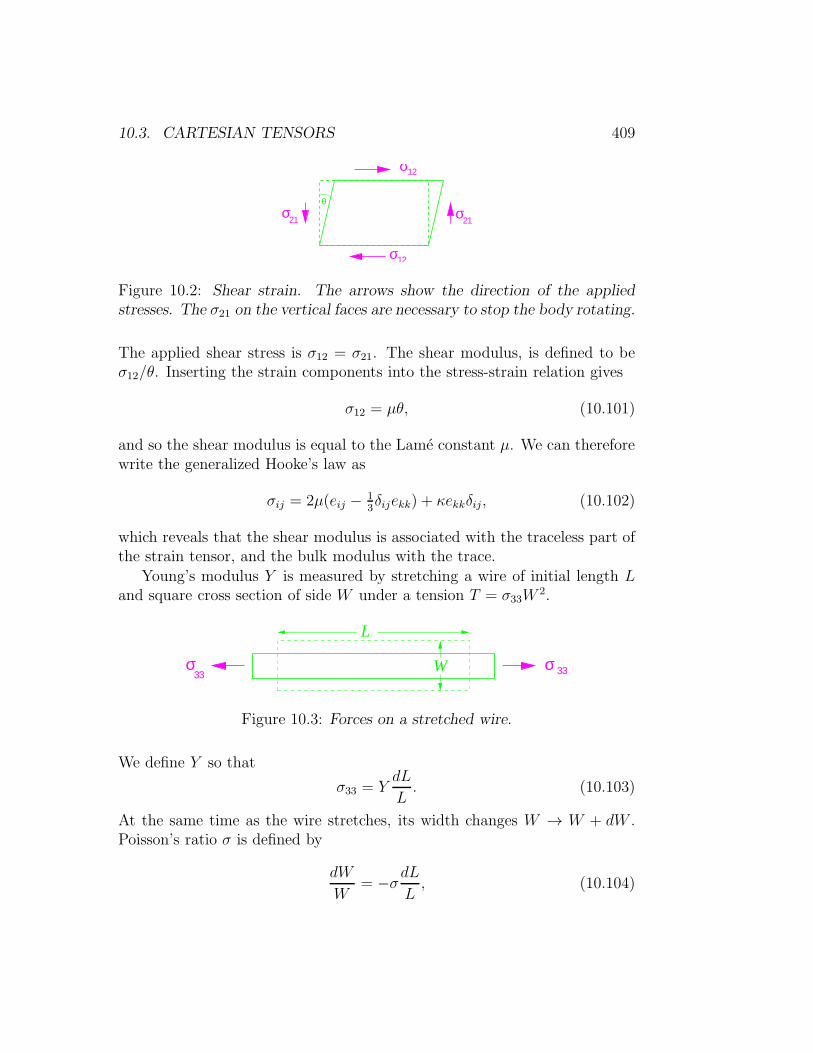
10.3. CARTESIAN TENSORS 409
σ21σ21
σ12
σ12
θ
Figure 10.2: Shear strain. The arrows show the direction of the appliedstresses. The σ21 on the vertical faces are necessary to stop the body rotating.
The applied shear stress is σ12 = σ21. The shear modulus, is defined to beσ12/θ. Inserting the strain components into the stress-strain relation gives
σ12 = µθ, (10.101)
and so the shear modulus is equal to the Lame constant µ. We can thereforewrite the generalized Hooke’s law as
σij = 2µ(eij − 13δijekk) + κekkδij, (10.102)
which reveals that the shear modulus is associated with the traceless part ofthe strain tensor, and the bulk modulus with the trace.
Young’s modulus Y is measured by stretching a wire of initial length Land square cross section of side W under a tension T = σ33W
2.
L
σ 33σ33
W
Figure 10.3: Forces on a stretched wire.
We define Y so that
σ33 = YdL
L. (10.103)
At the same time as the wire stretches, its width changes W → W + dW .Poisson’s ratio σ is defined by
dW
W= −σdL
L, (10.104)

410 CHAPTER 10. VECTORS AND TENSORS
so that σ is positive if the wire gets thinner as it gets longer. The displace-ments are
η3 = z
(dL
L
),
η1 = x
(dW
W
)= −σx
(dL
L
),
η2 = y
(dW
W
)= −σy
(dL
L
), (10.105)
so the strain components are
e33 =dL
L, e11 = e22 =
dW
W= −σe33. (10.106)
We therefore have
σ33 = (λ(1− 2σ) + 2µ)
(dL
L
), (10.107)
leading to
Y = λ(1− 2σ) + 2µ. (10.108)
Now, the side of the wire is a free surface with no forces acting on it, so
0 = σ22 = σ11 = (λ(1− 2σ)− 2σµ)
(dL
L
). (10.109)
This tells us that6
σ =1
2
λ
λ+ µ, (10.110)
and
Y = µ
(3λ+ 2µ
λ+ µ
). (10.111)
Other relations, following from those above, are
Y = 3κ(1− 2σ),
= 2µ(1 + σ). (10.112)
6Poisson and Cauchy erroneously believed that λ = µ, and hence that σ = 1/4.

10.3. CARTESIAN TENSORS 411
Γz
x
y
O
Figure 10.4: Bent beam.
Exercise 10.7: Show that the symmetries
cijkl = cklij = cjikl = cijlk
imply that a general homogeneous material has 21 independent elastic con-stants. (This result was originally obtained by George Green, of Green func-tion fame.)
Exercise 10.8: A steel beam is forged so that its cross section has the shapeof a region Γ ∈ R2. When undeformed, it lies along the z axis. The centroidO of each cross section is defined so that
∫
Γx dxdy =
∫
Γy dxdy = 0,
when the co-ordinates x, y are taken with the centroid O as the origin. Thebeam is slightly bent away from the z axis so that the line of centroids remainsin the y, z plane. (See figure 10.4) At a particular cross section with centroidO, the line of centroids has radius of curvature R.
Assume that the deformation in the vicinity of O is such that
ηx = − σRxy,
ηy =1
2R
σ(x2 − y2)− z2
,
ηz =1
Ryz.
Observe that for this assumed deformation, and for a positive Poisson ratio,the cross section deforms anticlastically — the sides bend up as the beambends down. This is shown in figure 10.5.
Compute the strain tensor resulting from the assumed deformation, and showthat its only non-zero components are
exx = − σRy, eyy = −
σ
Ry, ezz =
1
Ry.

412 CHAPTER 10. VECTORS AND TENSORS
O
Γ
x
y
Figure 10.5: The original (dashed) and anticlastically deformed (full) cross-section.
Next, show that
σzz =
(Y
R
)y,
and that all other components of the stress tensor vanish. Deduce from thisvanishing that the assumed deformation satisfies the free-surface boundarycondition, and so is indeed the way the beam responds when it is bent byforces applied at its ends.
The work done in bending the beam
∫
beam
1
2eijcijklekl d
3x
is stored as elastic energy. Show that for our bent rod this energy is equal to
∫Y I
2
(1
R2
)ds ≈
∫Y I
2(y′′)2dz,
where s is the arc-length taken along the line of centroids of the beam,
I =
∫
Γy2 dxdy
is the moment of inertia of the region Γ about the x axis, and y′′ denotesthe second derivative of the deflection of the beam with respect to z (whichapproximates the arc-length). This last formula for the strain energy has beenused in a number of our calculus-of-variations problems.

10.3. CARTESIAN TENSORS 413
y
z
Figure 10.6: The distribution of forces σzz exerted on the left-hand part ofthe bent rod by the material to its right.
10.3.3 Maxwell stress tensor
Consider a small cubical element of an elastic body. If the stress tensor wereposition independent, the external forces on each pair of opposing faces ofthe cube would be equal in magnitude but pointing in opposite directions.There would therefore be no net external force on the cube. When σij is notconstant then we claim that the total force acting on an infinitesimal elementof volume dV is
Fi = ∂jσij dV. (10.113)
To see that this assertion is correct, consider a finite region Ω with boundary∂Ω, and use the divergence theorem to write the total force on Ω as
F toti =
∫
∂Ω
σijnjd|S| =∫
Ω
∂jσijdV. (10.114)
Whenever the force-per-unit-volume fi acting on a body can be writtenin the form fi = ∂jσij , we refer to σij as a “stress tensor,” by analogy withstress in an elastic solid. As an example, let E and B be electric and magneticfields. For simplicity, initially assume them to be static. The force per unitvolume exerted by these fields on a distribution of charge ρ and current j is
f = ρE + j×B. (10.115)
From Gauss’ law ρ = divD, and with D = ǫ0E, we find that the force perunit volume due the electric field has components
ρEi = (∂jDj)Ei = ǫ0
(∂j(EiEj)− Ej ∂jEi
)
= ǫ0
(∂j(EiEj)− Ej ∂iEj
)
= ǫ0∂j
(EiEj −
1
2δij |E|2
). (10.116)

414 CHAPTER 10. VECTORS AND TENSORS
Here, in passing from the first line to the second, we have used the fact thatcurlE is zero for static fields, and so ∂jEi = ∂iEj . Similarly, using j = curlH,together with B = µ0H and divB = 0, we find that the force per unit volumedue the magnetic field has components
(j×B)i = µ0∂j
(HiHj −
1
2δij|H|2
). (10.117)
The quantity
σij = ǫ0
(EiEj −
1
2δij |E|2
)+ µ0
(HiHj −
1
2δij |H|2
)(10.118)
is called the Maxwell stress tensor . Its utility lies in in the fact that thetotal electromagnetic force on an isolated body is the integral of the Maxwellstress over its surface. We do not need to know the fields within the body.
Michael Faraday was the first to intuit a picture of electromagnetic stressesand attributed both a longitudinal tension and a mutual lateral repulsion tothe field lines. Maxwell’s tensor expresses this idea mathematically.
Exercise 10.9: Allow the fields in the preceding calculation to be time depen-dent. Show that Maxwell’s equations
curlE = −∂B∂t, divB = 0,
curlH = j+∂D
∂t, divD = ρ,
with B = µ0H, D = ǫ0E, and c = 1/√µ0ǫ0, lead to
(ρE + j×B)i +∂
∂t
1
c2(E×H)i
= ∂jσij .
The left-hand side is the time rate of change of the mechanical (first term)and electromagnetic (second term) momentum density. Observe that we canequivalently write
∂
∂t
1
c2(E ×H)i
+ ∂j(−σij) = −(ρE+ j×B)i,
and think of this a local field-momentum conservation law. In this interpre-tation −σij is thought of as the momentum flux tensor, its entries being theflux in direction j of the component of field momentum in direction i. Theterm on the right-hand side is the rate at which momentum is being suppliedto the electro-magnetic field by the charges and currents.

10.4. FURTHER EXERCISES AND PROBLEMS 415
10.4 Further Exercises and Problems
Exercise 10.10: Quotient theorem. Suppose that you have come up with somerecipe for generating an array of numbers T ijk in any co-ordinate frame, andwant to know whether these numbers are the components of a triply con-travariant tensor. Suppose further that you know that, given the componentsaij of an arbitrary doubly covariant tensor, the numbers
T ijkajk = vi
transform as the components of a contravariant vector. Show that T ijk doesindeed transform as a triply contravariant tensor. (The natural generalizationof this result to arbitrary tensor types is known as the quotient theorem.)
Exercise 10.11: Let T ij be the 3-by-3 array of components of a tensor. Showthat the quantities
a = T ii, b = T ijTji, c = T ijT
jkT
ki
are invariant. Further show that the eigenvalues of the linear map representedby the matrix T ij can be found by solving the cubic equation
λ3 − aλ2 + 1
2(a2 − b)λ− 1
6(a3 − 3ab+ 2c) = 0.
Exercise 10.12: Let the covariant tensor Rijkl possess the following symme-tries:
i) Rijkl = −Rjikl,ii) Rijkl = −Rijlk,iii) Rijkl +Riklj +Riljk = 0.
Use the properties i),ii), iii) to show that:
a) Rijkl = Rklij.b) If Rijklx
iyjxkyl = 0 for all vectors xi, yi, then Rijkl = 0.c) If Bij is a symmetric covariant tensor and set we Aijkl = BikBjl−BilBjk,
then Aijkl has the same symmetries as Rijkl.
Exercise 10.13: Write out Euler’s equation for fluid motion
v + (v · ∇)v = −∇h
in Cartesian tensor notation. Transform it into
v − v ×ω = −∇(1
2v2 + h
),

416 CHAPTER 10. VECTORS AND TENSORS
where ω = ∇×v is the vorticity. Deduce Bernoulli’s theorem, that for steady(v = 0) flow the quantity 1
2v2 + h is constant along streamlines.
Exercise 10.14: The elastic properties of an infinite homogeneous and isotropicsolid of density ρ are described by Lame constants λ and µ. Show that theequation of motion for small-amplitude vibrations is
ρ∂2ηi∂t2
= (λ+ µ)∂2ηj∂xi∂xj
+ µ∂2ηi∂x2j
.
Here ηi are the cartesian components of the displacement vector η(x, t) of theparticle initially at the point x. Seek plane wave solutions of the form
η = a expik · x− iωt,
and deduce that there are two possible types of wave: longitudinal “P-waves,”which have phase velocity
vP =
√λ+ 2µ
ρ,
and transverse “S-waves,” which have phase velocity
vS =
õ
ρ.
Exercise 10.15: Symmetric integration. Show that the n-dimensional integral
Iαβγδ =
∫dnk
(2π)n(kαkβkγkδ) f(k
2),
is equal toA(δαβδγδ + δαγδβδ + δαδδβγ)
where
A =1
n(n+ 2)
∫dnk
(2π)n(k2)2f(k2).
Similarly evaluate
Iαβγδǫ =
∫dnk
(2π)n(kαkβkγkδkǫ) f(k
2).
Exercise 10.16: Write down the most general three-dimensional isotropic ten-sors of rank two and three.

10.4. FURTHER EXERCISES AND PROBLEMS 417
In piezoelectric materials, the application of an electric field Ei induces amechanical strain that is described by a rank-two symmetric tensor
eij = dijkEk,
where dijk is a third-rank tensor that depends only on the material. Showthat eij can only be non-zero in an anisotropic material.
Exercise 10.17: In three dimensions, a rank-five isotropic tensor Tijklm is alinear combination of expressions of the form ǫi1i2i3δi4i5 for some assignmentof the indices i, j, k, l,m to the i1, . . . , i5. Show that, on taking into accountthe symmetries of the Kronecker and Levi-Civita symbols, we can constructten distinct products ǫi1i2i3δi4i5 . Only six of these are linearly independent,however. Show, for example, that
ǫijkδlm − ǫjklδim + ǫkliδjm − ǫlijδkm = 0,
and find the three other independent relations of this sort.7
(Hint: Begin by showing that, in three dimensions,
δi1i2i3i4i5i6i7i8
def=
∣∣∣∣∣∣∣∣
δi1i5 δi1i6 δi1i7 δi1i8δi2i5 δi2i6 δi2i7 δi2i8δi3i5 δi3i6 δi3i7 δi3i8δi4i5 δi4i6 δi4i7 δi4i8
∣∣∣∣∣∣∣∣= 0,
and contract with ǫi6i7i8 .)
Problem 10.18: The Plucker Relations. This problem provides a challengingtest of your understanding of linear algebra. It leads you through the task ofderiving the necessary and sufficient conditions for
A = Ai1...ik ei1 ∧ . . . ∧ eik ∈∧
kV
to be decomposable asA = f1 ∧ f2 ∧ . . . ∧ fk.
The trick is to introduce two subspaces of V ,
i) W , the smallest subspace of V such that A ∈ ∧kW ,ii) W ′ = v ∈ V : v ∧A = 0,
7Such relations are called syzygies . A recipe for constructing linearly independent basissets of isotropic tensors can be found in: G. F. Smith, Tensor , 19 (1968) 79-88.

418 CHAPTER 10. VECTORS AND TENSORS
and explore their relationship.
a) Show that if w1,w2, . . . ,wn constitute a basis for W ′, then
A = w1 ∧w2 ∧ · · · ∧wn ∧ϕ
for some ϕ ∈ ∧k−n V . Conclude that that W ′ ⊆ W , and that equal-ity holds if and only if A is decomposable, in which case W = W ′ =spanf1 . . . fk.
b) Now show that W is the image space of∧k−1 V ∗ under the map that
takesΞ = Ξi1...ik−1
e∗i1 ∧ . . . ∧ e∗ik−1 ∈∧
k−1V ∗
toi(Ξ)A
def= Ξi1...ik−1
Ai1...ik−1jej ∈ VDeduce that the condition W ⊆W ′ is that
(i(Ξ)A
)∧A = 0, ∀Ξ ∈
∧k−1V ∗.
c) By takingΞ = e∗i1 ∧ . . . ∧ e∗ik−1 ,
show that the condition in part b) can be written as
Ai1...ik−1j1Aj2j3...jk+1ej1 ∧ . . . ∧ ejk+1= 0.
Deduce that the necessary and sufficient conditions for decomposibilityare that
Ai1...ik−1[j1Aj2j3...jk+1] = 0,
for all possible index sets i1, . . . , ik−1, j1, . . . jk+1. Here [. . .] denotes anti-symmetrization of the enclosed indices.

Chapter 11
Differential Calculus onManifolds
In this section we will apply what we have learned about vectors and ten-sors in linear algebra to vector and tensor fields in a general curvilinearco-ordinate system. Our aim is to introduce the reader to the modern lan-guage of advanced calculus, and in particular to the calculus of differentialforms on surfaces and manifolds.
11.1 Vector and Covector Fields
Vector fields — electric, magnetic, velocity fields, and so on — appear every-where in physics. After perhaps struggling with it in introductory courses, werather take the field concept for granted. There remain subtleties, however.Consider an electric field. It makes sense to add two field vectors at a singlepoint, but there is no physical meaning to the sum of field vectors E(x1) andE(x2) at two distinct points. We should therefore regard all possible electricfields at a single point as living in a vector space, but each different point inspace comes with its own field-vector space.
This view seems even more reasonable when we consider velocity vectorsdescribing motion on a curved surface. A velocity vector lives in the tangentspace to the surface at each point, and each of these spaces is a differentlyoriented subspace of the higher-dimensional ambient space.
419

420 CHAPTER 11. DIFFERENTIAL CALCULUS ON MANIFOLDS
Figure 11.1: Each point on a surface has its own vector space of tangents.
Mathematicians call such a collection of vector spaces — one for each of thepoints in a surface — a vector bundle over the surface. Thus, the tangentbundle over a surface is the totality of all vector spaces tangent to the surface.Why a bundle? This word is used because the individual tangent spaces arenot completely independent, but are tied together in a rather non-obviousway. Try to construct a smooth field of unit vectors tangent to the surfaceof a sphere. However hard you work you will end up in trouble somewhere.You cannot comb a hairy ball. On the surface of torus you will have no suchproblems. You can comb a hairy doughnut. The tangent spaces collectivelyknow something about the surface they are tangent to.
Although we spoke in the previous paragraph of vectors tangent to acurved surface, it is useful to generalize this idea to vectors lying in thetangent space of an n-dimensional manifold , or n-manifold. A n-manifoldMis essentially a space that locally looks like a part of Rn. This means thatsome open neighbourhood of each point x ∈ M can be parametrized by ann-dimensional co-ordinate system. A co-ordinate parametrization is called achart . Unless M is Rn itself (or part of it), a chart will cover only part ofM , and more than one will be required for complete coverage. Where a pairof charts overlap, we demand that the transformation formula giving one setof co-ordinates as a function of the other be a smooth (C∞) function, and topossess a smooth inverse.1 A collection of such smoothly related co-ordinatecharts covering all of M is called an atlas . The advantage of thinking interms of manifolds is that we do not have to understand their propertiesas arising from some embedding in a higher dimensional space. Whateverstructure they have, they possess in, and of, themselves
1A formal definition of a manifold contains some further technical restrictions (that thespace be Hausdorff and paracompact) that are designed to eliminate pathologies. We aremore interested in doing calculus than in proving theorems, and so we will ignore theseniceties.

11.1. VECTOR AND COVECTOR FIELDS 421
Classical mechanics provides a familiar illustration of these ideas. Exceptin pathological cases, the configuration space M of a mechanical system isa manifold. When the system has n degrees of freedom we use generalizedco-ordinates qi, i = 1, . . . , n to parametrize M . The tangent bundle of Mthen provides the setting for Lagrangian mechanics. This bundle, denotedby TM , is the 2n-dimensional space each of whose whose points consists of apoint q = (q1, . . . , qn) in M paired with a tangent vector lying in the tangentspace TMq at that point. If we think of the tangent vector as a velocity, thenatural co-ordinates on TM become (q1, q2, . . . , qn ; q1, q2, . . . , qn), and theseare the variables that appear in the Lagrangian of the system.
If we consider a vector tangent to some curved surface, it will stick outof it. If we have a vector tangent to a manifold, it is a straight arrow lyingatop bent co-ordinates. Should we restrict the length of the vector so thatit does not stick out too far? Are we restricted to only infinitesimal vectors?It is best to avoid all this by adopting a clever notion of what a vector ina tangent space is. The idea is to focus on a well-defined object such asa derivative. Suppose that our space has co-ordinates xµ. (These are notthe contravariant components of some vector) A directional derivative is anobject such asXµ∂µ, where ∂µ is shorthand for ∂/∂xµ. When the componentsXµ are functions of the co-ordinates xσ, this object is called a tangent-vectorfield, and we write2
X = Xµ∂µ. (11.1)
We regard the ∂µ at a point x as a basis for TMx, the tangent-vector space atx, and the Xµ(x) as the (contravariant) components of the vector X at thatpoint. Although they are not little arrows, what the ∂µ are is mathematicallyclear, and so we know perfectly well how to deal with them.
When we change co-ordinate system from xµ to zν by regarding the xµ’sas invertable functions of the zν ’s, i.e.
x1 = x1(z1, z2, . . . , zn),
x2 = x2(z1, z2, . . . , zn),...
xn = xn(z1, z2, . . . , zn), (11.2)
2We are going to stop using bold symbols to distinguish between intrinsic objects andtheir components, because from now on almost everything will be something other than anumber, and too much black ink would just be confusing.

422 CHAPTER 11. DIFFERENTIAL CALCULUS ON MANIFOLDS
then the chain rule for partial differentiation gives
∂µ ≡∂
∂xµ=∂zν
∂xµ∂
∂zν=
(∂zν
∂xµ
)∂′ν , (11.3)
where ∂′ν is shorthand for ∂/∂zν . By demanding that
X = Xµ∂µ = X ′ν∂′ν (11.4)
we find the components in the zν co-ordinate frame to be
X ′ν =
(∂zν
∂xµ
)Xµ. (11.5)
Conversely, using∂xσ
∂zν∂zν
∂xµ=∂xσ
∂xµ= δσµ , (11.6)
we have
Xν =
(∂xν
∂zµ
)X ′µ. (11.7)
This, then, is the transformation law for a contravariant vector.It is worth pointing out that the basis vectors ∂µ are not unit vectors. As
we have no metric, and therefore no notion of length anyway, we cannot tryto normalize them. If you insist on drawing (small?) arrows, think of ∂1 asstarting at a point (x1, x2, . . . , xn) and with its head at (x1 + 1, x2, . . . , xn).Of course this is only a good picture if the co-ordinates are not too “curvy.”
x =2 x =3 x =4
x =5
x =4
x =6
1 1 1
2
2
2
2
1
Figure 11.2: Approximate picture of the vectors ∂1 and ∂2 at the point(x1, x2) = (2, 4).
Example: The surface of the unit sphere is a manifold. It is usually denotedby S2. We may label its points with spherical polar co-ordinates, θ mea-suring the co-latitude and φ measuring the longitude. These will be useful

11.1. VECTOR AND COVECTOR FIELDS 423
everywhere except at the north and south poles, where they become singularbecause at θ = 0 or π all values of of the longitude φ correspond to the samepoint. In this co-ordinate basis, the tangent vector representing the velocityfield due to a rigid rotation of one radian per second about the z axis is
Vz = ∂φ. (11.8)
Similarly
Vx = − sinφ ∂θ − cot θ cosφ ∂φ,
Vy = cosφ ∂θ − cot θ sinφ∂φ, (11.9)
respectively represent rigid rotations about the x and y axes.We now know how to think about vectors. What about their dual-space
partners, the covectors? These live in the cotangent bundle T ∗M , and forthem a cute notational game, due to Elie Cartan, is played. We write thebasis vectors dual to the ∂µ as dxµ( ). Thus
dxµ(∂ν) = δµν . (11.10)
When evaluated on a vector field X = Xµ∂µ, the basis covectors dxµ returnits components:
dxµ(X) = dxµ(Xν∂ν) = Xνdxµ(∂ν) = Xνδµν = Xµ. (11.11)
Now, any smooth function f ∈ C∞(M) will give rise to a field of covectorsin T ∗M . This is because a vector field X acts on the scalar function f as
Xf = Xµ∂µf (11.12)
and Xf is another scalar function. This new function gives a number — andthus an element of the field R — at each point x ∈ M . But this is exactlywhat a covector does: it takes in a vector at a point and returns a number.We will call this covector field “df .” It is essentially the gradient of f . Thus
df(X)def= Xf = Xµ ∂f
∂xµ. (11.13)
If we take f to be the co-ordinate xν , we have
dxν(X) = Xµ ∂xν
∂xµ= Xµδνµ = Xν , (11.14)

424 CHAPTER 11. DIFFERENTIAL CALCULUS ON MANIFOLDS
so this viewpoint is consistent with our previous definition of dxν . Thus
df(X) =∂f
∂xµXµ =
∂f
∂xµdxµ(X) (11.15)
for any vector field X . In other words, we can expand df as
df =∂f
∂xµdxµ. (11.16)
This is not some approximation to a change in f , but is an exact expansionof the covector field df in terms of the basis covectors dxµ.
We may retain something of the notion that dxµ represents the (con-travariant) components of a small displacement in x provided that we thinkof dxµ as a machine into which we insert the small displacement (a vector)and have it spit out the numerical components δxµ. This is the same dis-tinction that we make between sin( ) as a function into which one can plugx, and sin x, the number that results from inserting in this particular valueof x. Although seemingly innocent, we know that it is a distinction of greatpower.
The change of co-ordinates transformation law for a covector field fµ isfound from
fµ dxµ = f ′
ν dzν , (11.17)
by using
dxµ =
(∂xµ
∂zν
)dzν . (11.18)
We find
f ′ν =
(∂xµ
∂zν
)fµ. (11.19)
A general tensor such as Qλµρστ transforms as
Q′λµρστ (z) =
∂zλ
∂xα∂zµ
∂xβ∂xγ
∂zρ∂xδ
∂zσ∂xǫ
∂zτQαβ
γδǫ(x). (11.20)
Observe how the indices are wired up: Those for the new tensor coefficientsin the new co-ordinates, z, are attached to the new z’s, and those for the oldcoefficients are attached to the old x’s. Upstairs indices go in the numeratorof each partial derivative, and downstairs ones are in the denominator.

11.2. DIFFERENTIATING TENSORS 425
The language of bundles and sections
At the beginning of this section, we introduced the notion of a vector bundle.This is a particular example of the more general concept of a fibre bundle,where the vector space at each point in the manifold is replaced by a “fibre”over that point. The fibre can be any mathematical object, such as a set,tensor space, or another manifold. Mathematicians visualize the bundle asa collection of fibres growing out of the manifold, much as stalks of wheatgrow out the soil. When one slices through a patch of wheat with a scythe,the blade exposes a cross-section of the stalks. By analogy, a choice of anelement of the the fibre over each point in the manifold is called a cross-section, or, more commonly, a section of the bundle. In this language, atangent-vector field becomes a section of the tangent bundle, and a field ofcovectors becomes a section of the cotangent bundle.
We provide a more detailed account of bundles in Chapter 16.
11.2 Differentiating Tensors
If f is a function then ∂µf are components of the covariant vector df . Supposethat aµ is a contravariant vector. Are ∂νa
µ the components of a type (1, 1)tensor? The answer is no! In general, differentiating the components of atensor does not give rise to another tensor. One can see why at two levels:
a) Consider the transformation laws. They contain expressions of the form∂xµ/∂zν . If we differentiate both sides of the transformation law of atensor, these factors are also differentiated, but tensor transformationlaws never contain second derivatives, such as ∂2xµ/∂zν∂zσ .
b) Differentiation requires subtracting vectors or tensors at different points— but vectors at different points are in different vector spaces, so theirdifference is not defined.
These two reasons are really one and the same. We need to be cleverer toget new tensors by differentiating old ones.
11.2.1 Lie Bracket
One way to proceed is to note that the vector field X is an operator . It makessense, therefore, to try to compose two of them to make another. Look at

426 CHAPTER 11. DIFFERENTIAL CALCULUS ON MANIFOLDS
XY , for example:
XY = Xµ∂µ(Yν∂ν) = XµY ν∂2µν +Xµ
(∂Y ν
∂xµ
)∂ν . (11.21)
What are we to make of this? Not much! There is no particular interpretationfor the second derivative, and as we saw above, it does not transform nicely.But suppose we take a commutator :
[X, Y ] = XY − Y X = (Xµ(∂µYν)− Y µ(∂µX
ν)) ∂ν . (11.22)
The second derivatives have cancelled, and what remains is a directionalderivative and so a bona-fide vector field. The components
[X, Y ]ν ≡ Xµ(∂µYν)− Y µ(∂µX
ν) (11.23)
are the components of a new contravariant vector field made from the twoold vector fields. This new vector field is called the Lie bracket of the twofields, and has a geometric interpretation.
To understand the geometry of the Lie bracket, we first define the flowassociated with a tangent-vector field X . This is the map that takes a pointx0 and maps it to x(t) by solving the family of equations
dxµ
dt= Xµ(x1, x2, . . .), (11.24)
with initial condition xµ(0) = xµ0 . In words, we regard X as the velocity fieldof a flowing fluid, and let x ride along with the fluid.
Now envisage X and Y as two velocity fields. Suppose we flow along Xfor a brief time t, then along Y for another brief interval s. Next we switchback to X , but with a minus sign, for time t, and then to −Y for a finalinterval of s. We have tried to retrace our path, but a short exercise withTaylor’s theorem shows that we will fail to return to our exact starting point.We will miss by δxµ = st[X, Y ]µ, plus corrections of cubic order in s and t.(See figure 11.3)

11.2. DIFFERENTIATING TENSORS 427
−sYtX
sY
−tX
X,Y[ ]st
Figure 11.3: We try to retrace our steps but fail to return by a distanceproportional to the Lie bracket.
Example: Let
Vx = − sinφ ∂θ − cot θ cosφ ∂φ,
Vy = cosφ ∂θ − cot θ sinφ ∂φ,
be two vector fields in T (S2). We find that
[Vx, Vy] = −Vz,
where Vz = ∂φ.
Frobenius’ Theorem
Suppose that in some region of a d-dimensional manifold M we are givenn < d linearly independent tangent-vector fields Xi. Such a set is called adistribution by differential geometers. (The concept has nothing to do withprobability, or with objects like “δ(x)” which are also called “distributions.”)At each point x, the span 〈Xi(x)〉 of the field vectors forms a subspace ofthe tangent space TMx, and we can picture this subspace as a fragment ofan n-dimensional surface passing through x. It is possible that these surfacefragments fit together to make a stack of smooth surfaces — called a foliation— that fill out the d-dimensional space, and have the givenXi as their tangentvectors.

428 CHAPTER 11. DIFFERENTIAL CALCULUS ON MANIFOLDS
X 1X 2
x
N
Figure 11.4: A local foliation.
If this is the case then starting from x and taking steps only along the Xi
we find ourselves restricted to the n-surface, or n-submanifold , N passingthough the original point x.
Alternatively, the surface fragments may form such an incoherent jumblethat starting from x and moving only along the Xi we can find our way to anypoint in the neighbourhood of x. It is also possible that some intermediatecase applies, so that moving along the Xi restricts us to an m-surface, whered > m > n. The Lie bracket provides us with the appropriate tool withwhich to investigate these possibilities.
First a definition: If there are functions c kij (x) such that
[Xi, Xj] = c kij (x)Xk, (11.25)
i.e. the Lie brackets close within the set Xi at each point x, then thedistribution is said to be involutive. and the vector fields are said to be “ininvolution” with each other. When our given distribution is involutive, thenthe first case holds, and, at least locally, there is a foliation by n-submanifoldsN . A formal statement of this is:Theorem (Frobenius): A smooth (C∞) involutive distribution is completelyintegrable: locally, there are co-ordinates xµ, µ = 1, . . . , d such that Xi =∑n
µ=1Xµi ∂µ, and the surfaces N through each point are in the form xµ =
const. for µ = n + 1, . . . , d. Conversely, if such co-ordinates exist then thedistribution is involutive.A half-proof : If such co-ordinates exist then it is obvious that the Lie bracketof any pair of vectors in the form Xi =
∑nµ=1X
µi ∂µ can also be expanded in
terms of the first n basis vectors. A logically equivalent statement exploits thegeometric interpretation of the Lie bracket: If the Lie brackets of the fieldsXi do not close within the n-dimensional span of the Xi, then a sequenceof back-and-forth manœvres along the Xi allows us to escape into a new

11.2. DIFFERENTIATING TENSORS 429
direction, and so the Xi cannot be tangent to an n-surface. Establishing theconverse — that closure implies the existence of the foliation — is rathermore technical, and we will not attempt it.
Involutive and non-involutive distributions appear in classical mechanicsunder the guise of holonomic and anholonomic constraints. In mechanics,constraints are not usually given as a list of the directions (vector fields) inwhich we are free to move, but instead as a list of restrictions imposed on thepermitted motion. In a d-dimensional mechanical system we might have setof m independent constraints of the form ωiµ(q)q
µ = 0, i = 1, . . . , m. Suchrestrictions are most naturally expressed in terms of the covector fields
ωi =d∑
µ=1
ωiµ(q)dqµ, i = 1 ≤ i ≤ m. (11.26)
We can write the constraints as the m conditions ωi(q) = 0 that must besatisfied if q ≡ qµ∂µ is to be an allowed motion. The list of constraints isknown a Pfaffian system of equations. These equations indirectly determinean n = d −m dimensional distribution of permitted motions. The Pfaffiansystem is said to be integrable if this distribution is involutive, and henceintegrable. In this case there is a set of m functions gi(q) and an invertiblem-by-m matrix f ij(q) such that
ωi =
m∑
j=1
f ij(q)dgj. (11.27)
The functions gi(q) can, for example, be taken to be the co-ordinate functionsxµ, µ = n + 1, . . . , d, that label the foliating surfaces N in the statement ofFrobenius’ theorem. The system of integrable constraints ωi(q) = 0 thusrestricts us to the surfaces gi(q) = constant.
For example, consider a particle moving in three dimensions. If we aretold that the velocity vector is constrained by ω(q) = 0, where
ω = x dx+ y dy + z dz (11.28)
we realize that the particle is being forced to move on a sphere passingthrough the initial point. In spherical co-ordinates the associated distributionis the set ∂θ, ∂φ, which is clearly involutive because [∂θ, ∂φ] = 0. Thefunctions f(x, y, z) and g(x, y, z) from the previous paragraph can be taken
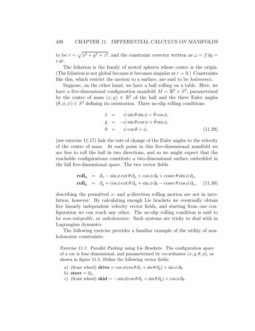
430 CHAPTER 11. DIFFERENTIAL CALCULUS ON MANIFOLDS
to be r =√x2 + y2 + z2, and the constraint covector written as ω = f dg =
r dr.The foliation is the family of nested spheres whose centre is the origin.
(The foliation is not global because it becomes singular at r = 0.) Constraintslike this, which restrict the motion to a surface, are said to be holonomic.
Suppose, on the other hand, we have a ball rolling on a table. Here, wehave a five-dimensional configuration manifold M = R2 × S3, parametrizedby the centre of mass (x, y) ∈ R2 of the ball and the three Euler angles(θ, φ, ψ) ∈ S3 defining its orientation. Three no-slip rolling conditions
x = ψ sin θ sinφ+ θ cosφ,
y = −ψ sin θ cosφ+ θ sin φ,
0 = ψ cos θ + φ, (11.29)
(see exercise 11.17) link the rate of change of the Euler angles to the velocityof the centre of mass. At each point in this five-dimensional manifold weare free to roll the ball in two directions, and so we might expect that thereachable configurations constitute a two-dimensional surface embedded inthe full five-dimensional space. The two vector fields
rollx = ∂x − sinφ cot θ ∂φ + cosφ ∂θ + cosec θ sin φ ∂ψ,
rolly = ∂y + cosφ cot θ ∂φ + sin φ ∂θ − cosec θ cosφ ∂ψ, (11.30)
describing the permitted x- and y-direction rolling motion are not in invo-lution, however. By calculating enough Lie brackets we eventually obtainfive linearly independent velocity vector fields, and starting from one con-figuration we can reach any other. The no-slip rolling condition is said tobe non-integrable, or anholonomic. Such systems are tricky to deal with inLagrangian dynamics.
The following exercise provides a familiar example of the utility of non-holonomic constraints:
Exercise 11.1: Parallel Parking using Lie Brackets. The configuration spaceof a car is four dimensional, and parameterized by co-ordinates (x, y, θ, φ), asshown in figure 11.5. Define the following vector fields:
a) (front wheel) drive = cosφ(cos θ ∂x + sin θ ∂y) + sinφ∂θ.b) steer = ∂φ.c) (front wheel) skid = − sinφ(cos θ ∂x + sin θ ∂y) + cosφ∂θ.

11.2. DIFFERENTIATING TENSORS 431
θ
(x,y)
drive
park
φ
Figure 11.5: Co-ordinates for car parking
d) park = − sin θ ∂x + cos θ ∂y.
Explain why these are apt names for the vector fields, and compute the sixLie brackets:
[steer,drive], [steer, skid], [skid,drive],
[park,drive], [park,park], [park, skid].
The driver can use only the operations (±)drive and (±) steer to manœvrethe car. Use the geometric interpretation of the Lie bracket to explain how asuitable sequence of motions (forward, reverse, and turning the steering wheel)can be used to manoeuvre a car sideways into a parking space.
11.2.2 Lie Derivative
Another derivative that we can define is the Lie derivative along a vectorfield X . It is defined by its action on a scalar function f as
LXf def= Xf, (11.31)
on a vector field by
LXY def= [X, Y ], (11.32)
and on anything else by requiring it to be a derivation, meaning that it obeysLeibniz’ rule. For example, let us compute the Lie derivative of a covector
432 CHAPTER 11. DIFFERENTIAL CALCULUS ON MANIFOLDS
F . We first introduce an arbitrary vector field Y and plug it into F to getthe scalar function F (Y ). Leibniz’ rule is then the statement that
LXF (Y ) = (LXF )(Y ) + F (LXY ). (11.33)
Since F (Y ) is a function and Y is a vector, both of whose derivatives weknow how to compute, we know the first and third of the three terms in thisequation. From LXF (Y ) = XF (Y ) and F (LXY ) = F ([X, Y ]), we have
XF (Y ) = (LXF )(Y ) + F ([X, Y ]), (11.34)
and so(LXF )(Y ) = XF (Y )− F ([X, Y ]). (11.35)
In components, this becomes
(LXF )(Y ) = Xν∂ν(FµYµ)− Fν(Xµ∂µY
ν − Y µ∂µXν)
= (Xν∂νFµ + Fν∂µXν)Y µ. (11.36)
Note how all the derivatives of Y µ have cancelled, so LXF ( ) depends onlyon the local value of Y . The Lie derivative of F is therefore still a covectorfield. This is true in general: the Lie derivative does not change the tensorcharacter of the objects on which it acts. Dropping the passive spectatorfield Y ν , we have a formula for LXF in components:
(LXF )µ = Xν∂νFµ + Fν∂µXν . (11.37)
Another example is provided by the Lie derivative of a type (0, 2) tensor,such as a metric tensor. This is
(LXg)µν = Xα∂αgµν + gµα∂νXα + gαν∂µX
α. (11.38)
The Lie derivative of a metric measures the extent to which the displacementxα → xα + ǫXα(x) deforms the geometry. If we write the metric as
g( , ) = gµν(x) dxµ ⊗ dxν , (11.39)
we can understand both this geometric interpretation and the origin of thethree terms appearing in the Lie derivative. We simply make the displace-ment xα → xα + ǫXα in the coefficients gµν(x) and in the two dxα. In thelatter we write
d(xα + ǫXα) = dxα + ǫ∂Xα
∂xβdxβ. (11.40)

11.2. DIFFERENTIATING TENSORS 433
Then we see that
gµν(x) dxµ ⊗ dxν → [gµν(x) + ǫ(Xα∂αgµν + gµα∂νX
α + gαν∂µXα)] dxµ ⊗ dxν
= [gµν + ǫ(LXg)µν ] dxµ ⊗ dxν . (11.41)
A displacement fieldX that does not change distances between points, i.e. onethat gives rise to an isometry , must therefore satisfy LXg = 0. Such an X issaid to be a Killing field after Wilhelm Killing who introduced them in hisstudy of non-euclidean geometries.
The geometric interpretation of the Lie derivative of a vector field is asfollows: In order to compute the X directional derivative of a vector field Y ,we need to be able to subtract the vector Y (x) from the vector Y (x + ǫX),divide by ǫ, and take the limit ǫ→ 0. To do this we have somehow to get thevector Y (x) from the point x, where it normally resides, to the new pointx + ǫX , so both vectors are elements of the same vector space. The Liederivative achieves this by carrying the old vector to the new point along thefield X .
Xεx
LεXε
YX
Y(x+εX)
Y(x)
Figure 11.6: Computing the Lie derivative of a vector.
Imagine the vector Y as drawn in ink in a flowing fluid whose velocity fieldis X . Initially the tail of Y is at x and its head is at x + Y . After flowingfor a time ǫ, its tail is at x + ǫX — i.e exactly where the tail of Y (x+ ǫX)lies. Where the head of transported vector ends up depends how the flow hasstretched and rotated the ink, but it is this distorted vector that is subtractedfrom Y (x+ ǫX) to get ǫLXY = ǫ[X, Y ].
Exercise 11.2: The metric on the unit sphere equipped with polar co-ordinatesis
g( , ) = dθ ⊗ dθ + sin2 θ dφ⊗ dφ.Consider
Vx = − sinφ∂θ − cot θ cosφ∂φ,
434 CHAPTER 11. DIFFERENTIAL CALCULUS ON MANIFOLDS
which is the vector field of a rigid rotation about the x axis. Compute the Liederivative LVxg, and show that it is zero.
Exercise 11.3: Suppose we have an unstrained block of material in real space.A co-ordinate system ξ1, ξ2, ξ3, is attached to the material of the body. Thepoint with co-ordinate ξ is located at (x1(ξ), x2(ξ), x3(ξ)) where x1, x2, x3 arethe usual R3 Cartesian co-ordinates.
a) Show that the induced metric in the ξ co-ordinate system is
gµν(ξ) =3∑
a=1
∂xa
∂ξµ∂xa
∂ξν.
b) The body is now deformed by an infinitesimal strain vector field η(ξ).The atom with co-ordinate ξµ is moved to what was ξµ+ηµ(ξ), or equiv-alently, the atom initially at Cartesian co-ordinate xa(ξ) is moved toxa + ηµ∂xa/∂ξµ. Show that the new induced metric is
gµν + δgµν = gµν + Lηgµν .
c) Define the strain tensor to be 1/2 of the Lie derivative of the metricwith respect to the deformation. If the original ξ co-ordinate systemcoincided with the Cartesian one, show that this definition reduces tothe familiar form
eab =1
2
(∂ηa∂xb
+∂ηb∂xa
),
all tensors being Cartesian.d) Part c) gave us the geometric definitition of infinitesimal strain. If the
body is deformed substantially, the Cauchy-Green finite strain tensor isdefined as
Eµν(ξ) =1
2
(gµν − g(0)µν
),
where g(0)µν is the metric in the undeformed body and gµν the metric in
the deformed body. Explain why this is a reasonable definition.
11.3 Exterior Calculus
11.3.1 Differential Forms
The objects we introduced in section 11.1, the dxµ, are called one-forms, ordifferential one-forms. They are fields living in the cotangent bundle T ∗M

11.3. EXTERIOR CALCULUS 435
of M . More precisely, they are sections of the cotangent bundle. Sectionsof the bundle whose fibre above x ∈ M is the p-th skew-symmetric tensorpower
∧p(T ∗Mx) of the cotangent space are known as p-forms.For example,
A = Aµdxµ = A1dx
1 + A2dx2 + A3dx
3, (11.42)
is a 1-form,
F =1
2Fµνdx
µ ∧ dxν = F12dx1 ∧ dx2 + F23dx
2 ∧ dx3 + F31dx3 ∧ dx1, (11.43)
is a 2-form, and
Ω =1
3!Ωµνσ dx
µ ∧ dxν ∧ dxσ = Ω123 dx1 ∧ dx2 ∧ dx3, (11.44)
is a 3-form. All the coefficients are skew-symmetric tensors, so, for example,
Ωµνσ = Ωνσµ = Ωσµν = −Ωνµσ = −Ωµσν = −Ωσνµ. (11.45)
In each example we have explicitly written out all the independent terms forthe case of three dimensions. Note how the p! disappears when we do thisand keep only distinct components. In d dimensions the space of p-forms isd!/p!(d− p)! dimensional, and all p-forms with p > d vanish identically.
As with the wedge products in chapter one, we regard a p-form as a p-linear skew-symetric function with p slots into which we can drop vectors toget a number. For example the basis two-forms give
dxµ ∧ dxν(∂α, ∂β) = δµαδνβ − δµβδνα. (11.46)
The analogous expression for a p-form would have p! terms. We can definean algebra of differential forms by “wedging” them together in the obviousway, so that the product of a p-form with a q-form is a (p + q)-form. Thewedge product is associative and distributive but not, of course, commuta-tive. Instead, if a is a p-form and b a q-form, then
a ∧ b = (−1)pq b ∧ a. (11.47)
Actually it is customary in this game to suppress the “∧” and simply writeF = 1
2Fµν dx
µdxν , it being assumed that you know that dxµdxν = −dxνdxµ— what else could it be?

436 CHAPTER 11. DIFFERENTIAL CALCULUS ON MANIFOLDS
11.3.2 The Exterior Derivative
These p-forms may seem rather complicated, so it is perhaps surprising thatall the vector calculus (div, grad, curl, the divergence theorem and Stokes’theorem, etc.) that you have learned in the past reduce, in terms of them,to two simple formulæ! Indeed Elie Cartan’s calculus of p-forms is slowlysupplanting traditional vector calculus, much as Willard Gibbs’ and OliverHeaviside’s vector calculus supplanted the tedious component-by-componentformulæ you find in Maxwell’s Treatise on Electricity and Magnetism.
The basic tool is the exterior derivative “d”, which we now define ax-iomatically:
i) If f is a function (0-form), then df coincides with the previous defini-tion, i.e. df(X) = Xf for any vector field X .
ii) d is an anti-derivation: If a is a p-form and b a q-form then
d(a ∧ b) = da ∧ b+ (−1)pa ∧ db. (11.48)
iii) Poincare’s lemma: d2 = 0, meaning that d(da) = 0 for any p-form a.iv) d is linear. That d(αa) = αda, for constant α follows already from i)
and ii), so the new fact is that d(a+ b) = da+ db.
It is not immediately obvious that axioms i), ii) and iii) are compatiblewith one another. If we use axiom i), ii) and d(dxi) = 0 to compute the d ofΩ = 1
p!Ωi1,...,ipdx
i1 · · · dxip , we find
dΩ =1
p!(dΩi1,...,ip) dx
i1 · · · dxip
=1
p!∂kΩi1,...,ip dx
kdxi1 · · · dxip . (11.49)
Now compute
d(dΩ) =1
p!
(∂l∂kΩi1,...,ip
)dxldxkdxi1 · · · dxip. (11.50)
Fortunately this is zero because ∂l∂kΩ = ∂k∂lΩ, while dxldxk = −dxkdxl.
As another example let A = A1dx1 + A2dx
2 + A3dx3, then
dA =
(∂A2
∂x1− ∂A1
∂x2
)dx1dx2 +
(∂A1
∂x3− ∂A3
∂x1
)dx3dx1 +
(∂A3
∂x2− ∂A2
∂x3
)dx2dx3
=1
2Fµνdx
µdxν , (11.51)

11.3. EXTERIOR CALCULUS 437
where
Fµν = ∂µAν − ∂νAµ. (11.52)
You will recognize the components of curlA hiding in here.Again, if F = F12dx
1dx2 + F23dx2dx3 + F31dx
3dx1 then
dF =
(∂F23
∂x1+∂F31
∂x2+∂F12
∂x3
)dx1dx2dx3. (11.53)
This looks like a divergence.The axiom d2 = 0 encompasses both “curl grad = 0” and “div curl =
0”, together with an infinite number of higher-dimensional analogues. Thefamiliar “curl =∇×”, meanwhile, is only defined in three dimensional space.
The exterior derivative takes p-forms to (p+1)-forms i.e. skew-symmetrictype (0, p) tensors to skew-symmetric (0, p + 1) tensors. How does “d” getaround the fact that the derivative of a tensor is not a tensor? Well, ifyou apply the transformation law for Aµ, and the chain rule to ∂
∂xµto find
the transformation law for Fµν = ∂µAν − ∂νAµ, you will see why: all thederivatives of the ∂zν
∂xµcancel, and Fµν is a bona-fide tensor of type (0, 2). This
sort of cancellation is why skew-symmetric objects are useful, and symmetricones less so.
Exercise 11.4: Use axiom ii) to compute d(d(a∧b)) and confirm that it is zero.
Closed and exact forms
The Poincare lemma, d2 = 0, leads to some important terminology:i) A p-form ω is said to be closed if dω = 0.ii) A p-form ω is said to exact if ω = dη for some (p− 1)-form η.
An exact form is necessarily closed, but a closed form is not necessarily exact.The question of when closed ⇒ exact is one involving the global topology ofthe space in which the forms are defined, and will be subject of chapter 13.
Cartan’s formulæ
It is sometimes useful to have expressions for the action of d coupled withthe evaluation of the subsequent (p+ 1) forms.
If f, η, ω, are 0, 1, 2-forms, respectively, then df, dη, dω, are 1, 2, 3-forms.When we plug in the appropriate number of vector fields X, Y, Z, then, after

438 CHAPTER 11. DIFFERENTIAL CALCULUS ON MANIFOLDS
some labour, we will find
df(X) = Xf. (11.54)
dη(X, Y ) = Xη(Y )− Y η(X)− η([X, Y ]). (11.55)
dω(X, Y, Z) = Xω(Y, Z) + Y ω(Z,X) + Zω(X, Y )
−ω([X, Y ], Z)− ω([Y, Z], X)− ω([Z,X ], Y ).(11.56)
These formulæ, and their higher-p analogues, express d in terms of geometricobjects, and so make it clear that the exterior derivative is itself a geometricobject, independent of any particular co-ordinate choice.
Let us demonstate the correctness of the second formula. With η = ηµdxµ,
the left-hand side, dη(X, Y ), is equal to
∂µην dxµdxν(X, Y ) = ∂µην(X
µY ν −XνY µ). (11.57)
The right hand side is equal to
Xµ∂µ(ηνYν)− Y µ∂µ(ηνX
ν)− ην(Xµ∂µYν − Y µ∂µX
ν). (11.58)
On using the product rule for the derivatives in the first two terms, we findthat all derivatives of the components of X and Y cancel, and are left withexactly those terms appearing on left.
Exercise 11.5: Let ωi, i = 1, . . . , r, be a linearly independent set of one-formsdefining a Pfaffian system (see sec. 11.2.1) in d dimensions.
i) Use Cartan’s formulæ to show that the corresponding (d−r)-dimensionaldistribution is involutive if and only if there is an r-by-r matrix of 1-formsθij such that
dωi =
r∑
j=1
θij ∧ ωj.
ii) Show that the conditions in part i) are satisfied if there are r functionsgi and an invertible r-by-r matrix of functions f ij such that
ωi =r∑
j=1
f ijdgi.
In this case foliation surfaces are given by the conditions gi(x) = const.,i = 1, . . . , r.

11.3. EXTERIOR CALCULUS 439
It is also possible, but considerably harder, to show that i) ⇒ ii). Doing sowould constitute a proof of Frobenius’ theorem.
Exercise 11.6: Let ω be a closed two-form, and let Null(ω) be the space ofvector fields X such that ω(X, ) = 0. Use the Cartan formulæ to show thatif X,Y ∈ Null(ω), then [X,Y ] ∈ Null(ω).
Lie Derivative of Forms
Given a p-form ω and a vector field X , we can form a (p − 1)-form callediXω by writing
iXω( . . . . . .︸ ︷︷ ︸p−1 slots
) = ω(
p slots︷ ︸︸ ︷X, . . . . . .︸ ︷︷ ︸
p−1 slots
). (11.59)
Acting on a 0-form, iX is defined to be 0. This procedure is called the interiormultiplication by X . It is simply a contraction
ωjij2...jp → ωkj2...jpXk, (11.60)
but it is convenient to have a special symbol for this operation. It is perhapssurprising that iX turns out to be an anti-derivation, just as is d. If η and ωare p and q forms respectively, then
iX(η ∧ ω) = (iXη) ∧ ω + (−1)pη ∧ (iXω), (11.61)
even though iX involves no differentiation. For example, if X = Xµ∂µ, then
iX(dxµ ∧ dxν) = dxµ ∧ dxν(Xα∂α, ),
= Xµdxν − dxµXν ,
= (iXdxµ) ∧ (dxν)− dxµ ∧ (iXdx
ν). (11.62)
One reason for introducing iX is that there is a nice (and profound)formula for the Lie derivative of a p-form in terms of iX . The formula iscalled the infinitesimal homotopy relation. It reads
LXω = (d iX + iXd)ω. (11.63)
This formula is proved by verifying that it is true for functions and one-forms, and then showing that it is a derivation – in other words that it

440 CHAPTER 11. DIFFERENTIAL CALCULUS ON MANIFOLDS
satisfies Leibniz’ rule. From the derivation property of the Lie derivative, weimmediately deduce that that the formula works for any p-form.
That the formula is true for functions should be obvious: Since iXf = 0by definition, we have
(d iX + iXd)f = iXdf = df(X) = Xf = LXf. (11.64)
To show that the formula works for one forms, we evaluate
(d iX + iXd)(fν dxν) = d(fνX
ν) + iX(∂µfν dxµdxν)
= ∂µ(fνXν)dxµ + ∂µfν(X
µdxν −Xνdxµ)
= (Xν∂νfµ + fν∂µXν)dxµ. (11.65)
In going from the second to the third line, we have interchanged the dummylabels µ ↔ ν in the term containing dxν . We recognize that the 1-form inthe last line is indeed LXf .
To show that diX + iXd is a derivation we must apply d iX + iXd to a∧ band use the anti-derivation property of ix and d. This is straightforward oncewe recall that d takes a p-form to a (p + 1)-form while iX takes a p-form toa (p− 1)-form.
Exercise 11.7: Let
ω =1
p!ωi1...ip dx
i1 · · · dxip .
Use the anti-derivation property of iX to show that
iXω =1
(p − 1)!ωαi2...ipX
αdxi2 · · · dxip ,
and so verify the equivalence of (11.59) and (11.60).
Exercise 11.8: Use the infinitesimal homotopy relation to show that L and dcommute, i.e. for ω a p-form, we have
d (LXω) = LX(dω).

11.4. PHYSICAL APPLICATIONS 441
11.4 Physical Applications
11.4.1 Maxwell’s Equations
In relativistic3 four-dimensional tensor notation the two source-free Maxwell’sequations
curlE = −∂B∂t,
divB = 0, (11.66)
reduce to the single equation
∂Fµν∂xλ
+∂Fνλ∂xµ
+∂Fλµ∂xν
= 0. (11.67)
where
Fµν =
0 −Ex −Ey −EzEx 0 Bz −By
Ey −Bz 0 Bx
Ez By −Bx 0
. (11.68)
The “F” is traditional, for Michael Faraday. In form language, the relativisticequation becomes the even more compact expression dF = 0, where
F ≡ 1
2Fµνdx
µdxν
= Bxdydz +Bydzdx+Bzdxdy + Exdxdt+ Eydydt+ Ezdzdt,
(11.69)
is a Minkowski-space 2-form.
Exercise 11.9: Verify that the source-free Maxwell equations are indeed equiv-alent to dF = 0.
The equation dF = 0 is automatically satisfied if we introduce a 4-vector1-form potential A = −φdt+ Axdx+ Aydy + Azdz and set F = dA.
The two Maxwell equations with sources
divD = ρ,
curlH = j +∂D
∂t, (11.70)
3In this section we will use units in which c = ǫ0 = µ0 = 1. We take the Minkowskimetric to be gµν = diag (−1, 1, 1, 1) where x0 = t, x1 = x , etc.

442 CHAPTER 11. DIFFERENTIAL CALCULUS ON MANIFOLDS
reduce in 4-tensor notation to the single equation
∂µFµν = Jν . (11.71)
Here Jµ = (ρ, j) is the current 4-vector.This source equation takes a little more work to express in form language,
but it can be done. We need a new concept: the Hodge “star” dual of a form.In d dimensions the “⋆” map takes a p-form to a (d − p)-form. It dependson both the metric and the orientation. The latter means a canonical choiceof the order in which to write our basis forms, with orderings that differby an even permutation being counted as the same. The full d-dimensionaldefinition involves the Levi-Civita duality operation of chapter 10 , combinedwith the use of the metric tensor to raise indices. Recall that
√g =
√det gµν .
(In Minkowski-signature metrics we should replace√g by
√−g.) We define“⋆” to be a linear map
⋆ :
p∧(T ∗M)→
(d−p)∧(T ∗M) (11.72)
such that
⋆ dxi1 . . . dxipdef=
1
(d− p)!√ggi1j1 . . . gipjpǫj1···jpjp+1···jddx
jp+1 . . . dxjd. (11.73)
Although this definition looks a trifle involved, computations involving it arenot so intimidating. The trick is to work, whenever possible, with orientedorthonormal frames. If we are in euclidean space and e∗i1 , e∗i2, . . . , e∗id is anordering of the orthonormal basis for (T ∗M)x whose orientation is equivalentto e∗1, e∗2, . . . , e∗d then
⋆ (e∗i1 ∧ e∗i2 ∧ · · · ∧ e∗ip) = e∗ip+1 ∧ e∗ip+2 ∧ · · · ∧ e∗id. (11.74)
For example, in three dimensions, and with x, y, z, our usual Cartesian co-ordinates, we have
⋆ dx = dydz,
⋆ dy = dzdx,
⋆ dz = dxdy. (11.75)
An analogous method works for Minkowski-signature (−,+,+,+) metrics,except that now we must include a minus sign for each negatively normed

11.4. PHYSICAL APPLICATIONS 443
dt factor in the form being “starred.” Taking dt, dx, dy, dz as our orientedbasis, we therefore find4
⋆ dxdy = −dzdt,⋆ dydz = −dxdt,⋆ dzdx = −dydt,⋆ dxdt = dydz,
⋆ dydt = dzdx,
⋆ dzdt = dxdy. (11.76)
For example, the first of these equations is derived by observing that (dxdy)(−dzdt) =dtdxdydz, and that there is no “dt” in the product dxdy. The fourth fol-lows from observing that that (dxdt)(−dydx) = dtdxdydz, but there is anegative-normed “dt” in the product dxdt.
The ⋆ map is constructed so that if
α =1
p!αi1i2...ipdx
i1dxi2 · · · dxip , (11.77)
and
β =1
p!βi1i2...ipdx
i1dxi2 · · · dxip, (11.78)
thenα ∧ (⋆β) = β ∧ (⋆α) = 〈α, β〉σ, (11.79)
where the inner product 〈α, β〉 is defined to be the invariant
〈α, β〉 = 1
p!gi1j1gi2j2 · · · gipjpαi1i2...ipβj1j2...jp, (11.80)
and σ is the volume form
σ =√g dx1dx2 · · · dxd. (11.81)
In future we will write α ⋆ β for α ∧ (⋆β). Bear in mind that the “⋆” in thisexpression is acting β and is not some new kind of binary operation.
We now apply these ideas to Maxwell. From the field-strength 2-form
F = Bxdydz +Bydzdx+Bzdxdy + Exdxdt+ Eydydt+ Ezdzdt, (11.82)
4See for example: Misner, Thorn and Wheeler, Gravitation, (MTW) page 108.

444 CHAPTER 11. DIFFERENTIAL CALCULUS ON MANIFOLDS
we get a dual 2-form
⋆F = −Bxdxdt− Bydydt− Bzdzdt+ Exdydz + Eydzdx+ Ezdxdy. (11.83)
We can check that we have correctly computed the Hodge star of F by takingthe wedge product, for which we find
F ⋆ F =1
2(FµνF
µν)σ = (B2x +B2
y +B2z − E2
x − E2y − E2
z )dtdxdydz. (11.84)
Observe that the expression B2−E2 is a Lorentz scalar. Similarly, from thecurrent 1-form
J ≡ Jµdxµ = −ρ dt+ jxdx+ jydy + jzdz, (11.85)
we derive the dual current 3-form
⋆J = ρ dxdydz − jxdtdydz − jydtdzdx− jzdtdxdy, (11.86)
and check that
J ⋆ J = (JµJµ)σ = (−ρ2 + j2x + j2y + j2z )dtdxdydz. (11.87)
Observe that
d ⋆ J =
(∂ρ
∂t+ div j
)dtdxdydz = 0, (11.88)
expresses the charge conservation law.Writing out the terms explicitly shows that the source-containing Maxwell
equations reduce to d⋆F = ⋆J. All four Maxwell equations are therefore verycompactly expressed as
dF = 0, d ⋆ F = ⋆J.
Observe that current conservation d⋆J = 0 follows from the second Maxwellequation as a consequence of d2 = 0.
Exercise 11.10: Show that for a p-form ω in d euclidean dimensions we have
⋆ ⋆ ω = (−1)p(d−p)ω.
Show, further, that for a Minkowski metric an additional minus sign has to beinserted. (For example, ⋆ ⋆ F = −F , even though (−1)2(4−2) = +1.)

11.4. PHYSICAL APPLICATIONS 445
11.4.2 Hamilton’s Equations
Hamiltonian dynamics takes place in phase space, a manifold with co-ordinates(q1, . . . , qn, p1, . . . , pn). Since momentum is a naturally covariant vector,5
phase space is usually the co-tangent bundle T ∗M of the configuration man-ifold M . We are writing the indices on the p’s upstairs though, because weare considering them as co-ordinates in T ∗M .
We expect that you are familiar with Hamilton’s equation in their q, psetting. Here, we shall describe them as they appear in a modern book onMechanics, such as Abrahams and Marsden’s Foundations of Mechanics, orV. I. Arnold’s Mathematical Methods of Classical Mechanics .
Phase space is an example of a symplectic manifold, a manifold equippedwith a symplectic form — a closed, non-degenerate, 2-form field
ω =1
2ωijdx
idxj . (11.89)
Recall that the word closed means that dω = 0. Non-degenerate means thatfor any point x the statement that ω(X, Y ) = 0 for all vectors Y ∈ TMx
implies that X = 0 at that point (or equivalently that for all x the matrixωij(x) has an inverse ωij(x)).
Given a Hamiltonian function H on our symplectic manifold, we definea velocity vector-field vH by solving
dH = −ivHω = −ω(vH , ) (11.90)
for vH . If the symplectic form is ω = dp1dq1 + dp2dq2 + · · ·+ dpndqn, this isnothing but a fancy form of Hamilton’s equations. To see this, we write
dH =∂H
∂qidqi +
∂H
∂pidpi (11.91)
and use the customary notation (qi, pi) for the velocity-in-phase-space com-ponents, so that
vH = qi∂
∂qi+ pi
∂
∂pi. (11.92)
Now we work out
ivHω = dpidqi(qj∂qj + pj∂pj , )
= pidqi − qidpi, (11.93)
5To convince yourself of this, remember that in quantum mechanics pµ = −i~ ∂∂xµ , and
the gradient of a function is a covector.

446 CHAPTER 11. DIFFERENTIAL CALCULUS ON MANIFOLDS
so, comparing coefficients of dpi and dqi on the two sides of dH = −ivHω, weread off
qi =∂H
∂pi, pi = −∂H
∂qi. (11.94)
Darboux’ theorem, which we will not try to prove, says that for any point xwe can always find co-ordinates p, q, valid in some neigbourhood of x, suchthat ω = dp1dq1+dp2dq2+ · · · dpndqn. Given this fact, it is not unreasonableto think that there is little to gained by using the abstract differential-formlanguage. In simple cases this is so, and the traditional methods are fine.It may be, however, that the neigbourhood of x where the Darboux co-ordinates work is not the entire phase space, and we need to cover the spacewith overlapping p, q co-ordinate charts. Then, what is a p in one chartwill usually be a combination of p’s and q’s in another. In this case, thetraditional form of Hamilton’s equations loses its appeal in comparison tothe co-ordinate-free dH = −ivHω.
Given two functions H1, H2 we can define their Poisson bracket H1, H2.Its importance lies in Dirac’s observation that the passage from classicalmechanics to quantum mechanics is accomplished by replacing the Poissonbracket of two quantities, A and B, with the commutator of the correspond-ing operators A, and B:
i[A, B] ←→ ~A,B+O(~2). (11.95)
We define the Poisson bracket by6
H1, H2 def=
dH2
dt
∣∣∣∣H1
= vH1H2. (11.96)
Now, vH1H2 = dH2(vH1
), and Hamilton’s equations say that dH2(vH1) =
ω(vH1, vH2
). Thus,H1, H2 = ω(vH1
, vH2). (11.97)
The skew symmetry of ω(vH1, vH2
) shows that despite the asymmetrical ap-pearance of the definition we have skew symmetry: H1, H2 = −H2, H1.
Moreover, since
vH1(H2H3) = (vH1
H2)H3 +H2(vH1H3), (11.98)
6Our definition differs in sign from the traditional one, but has the advantage of mini-mizing the number of minus signs in subsequent equations.

11.4. PHYSICAL APPLICATIONS 447
the Poisson bracket is a derivation:
H1, H2H3 = H1, H2H3 +H2H1, H3. (11.99)
Neither the skew symmetry nor the derivation property require the con-dition that dω = 0. What does need ω to be closed is the Jacobi identity :
H1, H2, H3+ H2, H3, H1+ H3, H1, H2 = 0. (11.100)
We establish Jacobi by using Cartan’s formula in the form
dω(vH1, vH2
, vH3) = vH1
ω(vH2, vH3
) + vH2ω(vH3
, vH1) + vH3
ω(vH1, vH2
)
−ω([vH1, vH2
], vH3)− ω([vH2
, vH3], vH1
)− ω([vH3, vH1
], vH2).
(11.101)
It is relatively straight-forward to interpret each term in the first of theselines as Poisson brackets. For example,
vH1ω(vH2
, vH3) = vH1
H2, H3 = H1, H2, H3. (11.102)
Relating the terms in the second line to Poisson brackets requires a littlemore effort. We proceed as follows:
ω([vH1, vH2
], vH3) = −ω(vH3
, [vH1, vH2
])
= dH3([vH1, vH2
])
= [vH1, vH2
]H3
= vH1(vH2
H3)− vH2(vH1
H3)
= H1, H2, H3 − H2, H1, H3= H1, H2, H3+ H2, H3, H1. (11.103)
Adding everything togther now shows that
0 = dω(vH1, vH2
, vH3)
= −H1, H2, H3 − H2, H3, H1 − H3, H1, H2.(11.104)
If we rearrange the Jacobi identity as
H1, H2, H3 − H2, H1, H3 = H1, H2, H3, (11.105)

448 CHAPTER 11. DIFFERENTIAL CALCULUS ON MANIFOLDS
we see that it is equivalent to
[vH1, vH2
] = vH1,H2.
The algebra of Poisson brackets is therefore homomorphic to the algebra ofthe Lie brackets. The correspondence is not an isomorphism, however: theassignment H 7→ vH fails to be one-to-one because constant functions mapto the zero vector field.
Exercise 11.11: Use the infinitesimal homotopy relation, to show that LvHω =0, where vH is the vector field corresponding toH. Suppose now that the phasespace is 2n dimensional. Show that in local Darboux co-ordinates the 2n-formωn/n! is, up to a sign, the phase-space volume element dnp dnq. Show thatLvHωn/n! = 0 and that this result is Liouville’s theorem on the conservationof phase-space volume.
The classical mechanics of spin
It is sometimes said in books on quantum mechanics that the spin of an elec-tron, or other elementary particle, is a purely quantum concept and cannotbe described by classical mechanics. This statement is false, but spin is thesimplest system in which traditional physicist’s methods become ugly and ithelps to use the modern symplectic language. A “spin” S can be regardedas a fixed length vector that can point in any direction in R3. We will takeit to be of unit length so that its components are
Sx = sin θ cosφ,
Sy = sin θ sinφ,
Sz = cos θ, (11.106)
where θ and φ are polar co-ordinates on the two-sphere S2.The surface of the sphere turns out to be both the configuration space
and the phase space. In particular the phase space for a spin is not thecotangent bundle of the configuration space. This has to be so: we learnedfrom Niels Bohr that a 2n-dimensional phase space contains roughly onequantum state for every ~n of phase-space volume. A cotangent bundlealways has infinite volume, so its corresponding Hilbert space is necessarilyinfinite dimensional. A quantum spin, however, has a finite-dimensionalHilbert space so its classical phase space must have a finite total volume.

11.4. PHYSICAL APPLICATIONS 449
This finite-volume phase space seems un-natural in the traditional view ofmechanics, but it fits comfortably into the modern symplectic picture.
We want to treat all points on the sphere alike, and so it is natural totake the symplectic 2-form to be proportional to the element of area. Supposethat ω = sin θ dθdφ. We could write ω = −d cos θ dφ and regard φ as “q”and − cos θ as “p” (Darboux’ theorem in action!), but this identification issingular at the north and south poles of the sphere, and, besides, it obscuresthe spherical symmetry of the problem, which is manifest when we think ofω as d(area).
Let us take our hamiltonian to be H = BSx, corresponding to an appliedmagnetic field in the x direction, and see what Hamilton’s equations give forthe motion. First we take the exterior derivative
d(BSx) = B(cos θ cosφdθ − sin θ sinφdφ). (11.107)
This is to be set equal to
−ω(vBSx , ) = vθ(− sin θ)dφ+ vφ sin θdθ. (11.108)
Comparing coefficients of dθ and dφ, we get
v(BSx) = vθ∂θ + vφ∂φ = B(sin φ∂θ + cosφ cot θ∂φ), (11.109)
i.e. B times the velocity vector for a rotation about the x axis. This velocityfield therefore describes a steady Larmor precession of the spin about theapplied field. This is exactly the motion predicted by quantum mechanics.Similarly, setting B = 1, we find
vSy = − cosφ∂θ + sin φ cot θ∂φ,
vSz = −∂φ. (11.110)
From these velocity fields we can compute the Poisson brackets:
Sx, Sy = ω(vSx, vSy)
= sin θdθdφ(sinφ∂θ + cos φ cot θ∂φ,− cosφ∂θ + sinφ cot θ∂φ)
= sin θ(sin2 φ cot θ + cos2 φ cot θ)
= cos θ = Sz.
Repeating the exercise leads to
Sx, Sy = Sz,
Sy, Sz = Sx,
Sz, Sx = Sy. (11.111)

450 CHAPTER 11. DIFFERENTIAL CALCULUS ON MANIFOLDS
These Poisson brackets for our classical “spin” are to be compared with thecommutation relations [Sx, Sy] = i~Sz etc. for the quantum spin operators
Si.
11.5 Covariant Derivatives
Covariant derivatives are a general class of derivatives that act on sectionsof a vector or tensor bundle over a manifold. We will begin by consideringderivatives on the tangent bundle, and in the exercises indicate how the ideageneralizes to other bundles.
11.5.1 Connections
The Lie and exterior derivatives require no structure beyond that whichcomes for free with our manifold. Another type of derivative that can act ontangent-space vectors and tensors is the covariant derivative ∇X ≡ Xµ∇µ.This requires an additional mathematical object called an affine connection.
The covariant derivative is defined by:i) Its action on scalar functions as
∇Xf = Xf. (11.112)
ii) Its action a basis set of tangent-vector fields ea(x) = eµa(x)∂µ (a localframe, or vielbein7) by introducing a set of functions ωijk(x) and, for
X = Xkek ≡ Xµ∂µ, setting
∇Xej = eiωijµX
µ = eiωijkX
k. (11.113)
ii) Extending this definition to any other type of tensor by requiring ∇X
to be a derivation.iii) Requiring that the result of applying ∇X to a tensor is a tensor of the
same type.The set of functions ωijk(x) is the connection. In any local co-ordinate chartwe can choose them at will, and different choices define different covariantderivatives. (There may be global compatibility constraints, however, whichappear when we assemble the charts into an atlas.)
7In practice viel , “many”, is replaced by the appropriate German numeral: ein-, zwei-,drei-, vier-, funf-, . . ., indicating the dimension. The word bein means “leg.”

11.5. COVARIANT DERIVATIVES 451
Warning: Despite having the appearance of one, ωijk is not a tensor. Ittransforms inhomogeneously under a change of frame or co-ordinates — seeequation (11.132).
We can, of course, take as our basis vectors the co-ordinate vectors eµ ≡∂µ. When we do this it is traditional to use the symbol Γ for the co-ordinateframe connection instead of ω. Thus,
∇µeν ≡ ∇eµeν = eλΓλνµ. (11.114)
The numbers Γλνµ are often called Christoffel symbols .As an example consider the covariant derivative of a vector f νeν . Using
the derivation property we have
∇µ(fνeν) = (∂µf
ν)eν + f ν∇µeν
= (∂µfν)eν + f νeλΓ
λνµ
= eν∂µf
ν + fλΓνλµ. (11.115)
In the first line we have used the defining property that ∇eµ acts on thefunctions f ν as ∂µ, and in the last line we interchanged the dummy indicesν and λ. We often abuse the notation by writing only the components, andset
∇µfν = ∂µf
ν + fλΓνλµ. (11.116)
Similarly, acting on the components of a mixed tensor, we would write
∇µAαβγ = ∂µA
αβγ + ΓαλµA
λβγ − ΓλβµA
αλγ − ΓλγµA
αβλ. (11.117)
When we use this notation, we are no longer regarding the tensor componentsas “functions.”
Observe that the plus and minus signs in (11.117) are required so that,for example, the covariant derivative of the scalar function fαg
α is
∇µ (fαgα) = ∂µ (fαg
α)
= (∂µfα) gα + fα (∂µg
α)
=(∂µfα − fλΓλαµ
)gα + fα
(∂µg
α + gλΓαλµ)
= (∇µfα) gα + fα (∇µg
α) , (11.118)
and so satisfies the derivation property.

452 CHAPTER 11. DIFFERENTIAL CALCULUS ON MANIFOLDS
Parallel transport
We have defined the covariant derivative via its formal calculus properties.It has, however, a geometrical interpretation. As with the Lie derivative, inorder to compute the derivative along X of the vector field Y , we have tosomehow carry the vector Y (x) from the tangent space TMx to the tangentspace TMx+ǫX , where we can subtract it from Y (x+ǫX) . The Lie derivativecarries Y along with the X flow. The covariant derivative implicitly carriesY by “parallel transport”. If γ : s 7→ xµ(s) is a parameterized curve withtangent vector Xµ∂µ, where
Xµ =dxµ
ds, (11.119)
then we say that the vector field Y (xµ(s)) is parallel transported along thecurve γ if
∇XY = 0, (11.120)
at each point xµ(s). Thus, a vector that in the vielbein frame ei at x hascomponents Y i will, after being parallel transported to x+ ǫX , end up com-ponents
Y i − ǫωijkY jXk. (11.121)
In a co-ordinate frame, after parallel transport through an infinitesimal dis-placement δxµ, the vector Y ν∂ν will have components
Y ν → Y ν − ΓνλµYλδxµ, (11.122)
and so
δxµ∇µYν = Y ν(xµ + δxµ)− Y ν(x)− ΓνλµY
λδxµ= δxµ∂µY ν + ΓνλµY
λ. (11.123)
Curvature and Torsion
As we said earlier, the connection ωijk(x) is not itself a tensor. Two importantquantities which are tensors, are associated with ∇X :
i) The torsionT (X, Y ) = ∇XY −∇YX − [X, Y ]. (11.124)
The quantity T (X, Y ) is a vector depending linearly on X, Y , so T atthe point x is a map TMx × TMx → TMx, and so a tensor of type(1,2). In a co-ordinate frame it has components
T λµν = Γλνµ − Γλµν . (11.125)

11.5. COVARIANT DERIVATIVES 453
ii) The Riemann curvature tensor
R(X, Y )Z = ∇X∇Y Z −∇Y∇XZ −∇[X,Y ]Z. (11.126)
The quantity R(X, Y )Z is also a vector, so R(X, Y ) is a linear mapTMx → TMx, and thus R itself is a tensor of type (1,3). Written outin a co-ordinate frame, we have
Rαβµν = ∂µΓ
αβν − ∂νΓαβµ + ΓαλµΓ
λβν − ΓαλνΓ
λβµ. (11.127)
If our manifold comes equipped with a metric tensor gµν (and is thusa Riemann manifold), and if we require both that T = 0 and ∇µgαβ = 0,then the connection is uniquely determined, and is called the Riemann, orLevi-Civita, connection. In a co-ordinate frame it is given by
Γαµν =1
2gαλ (∂µgλν + ∂νgµλ − ∂λgµν) . (11.128)
This is the connection that appears in General Relativity.The curvature tensor measures the degree of path dependence in parallel
transport: if Y ν(x) is parallel transported along a path γ : s 7→ xµ(s) froma to b, and if we deform γ so that xµ(s)→ xµ(s) + δxµ(s) while keeping theendpoints a, b fixed, then
δY α(b) = −∫ b
a
Rαβµν(x)Y
β(x)δxµ dxν . (11.129)
If Rαβµν ≡ 0 then the effect of parallel transport from a to b will be indepen-
dent of the route taken.The geometric interpretation of Tµν is less transparent. On a two-dimensional
surface a connection is torsion free when the tangent space “rolls withoutslipping” along the curve γ.
Exercise 11.12: Metric compatibility . Show that the Riemann connection
Γαµν =1
2gαλ (∂µgλν + ∂νgµλ − ∂λgµν) .
follows from the torsion-free condition Γαµν = Γανµ together with the metriccompatibility condition
∇µgαβ ≡ ∂µ gαβ − Γναµ gνβ − Γναµ gαν = 0.
Show that “metric compatibility” means that that the operation of raising orlowering indices commutes with covariant derivation.

454 CHAPTER 11. DIFFERENTIAL CALCULUS ON MANIFOLDS
Exercise 11.13: Geodesic equation. Let γ : s 7→ xµ(s) be a parametrizedpath from a to b. Show that the Euler-Lagrange equation that follows fromminimizing the distance functional
S(γ) =
∫ b
a
√gµν xµxν ds,
where the dots denote differentiation with respect to the parameter s, is
d2xµ
ds2+ Γµαβ
dxα
ds
dxβ
ds= 0.
Here Γµαβ is the Riemann connection (11.128).
Exercise 11.14: Show that if Aµ is a vector field then, for the Riemann con-nection,
∇µAµ =1√g
∂√gAµ
∂xµ.
In other words, show that
Γααµ =1√g
∂√g
∂xµ.
Deduce that the Laplacian acting on a scalar field φ can be defined by settingeither
∇2φ = gµν∇µ∇νφ,or
∇2φ =1√g
∂
∂xµ
(√ggµν
∂φ
∂xν
),
the two definitions being equivalent.
11.5.2 Cartan’s Form Viewpoint
Let e∗j(x) = e∗jµ(x)dxµ be the basis of one-forms dual to the vielbein frame
ei(x) = eµi (x)∂µ. Sinceδij = e∗i(ej) = e∗jµe
µi , (11.130)
the matrices e∗jµ and eµi are inverses of one-another. We can use them tochange from roman vielbein indices to greek co-ordinate frame indices. Forexample:
gij = g(ei, ej) = eµi gµνeνj , (11.131)

11.5. COVARIANT DERIVATIVES 455
andωijk = e∗iν(∂µe
νj )e
µk + e∗iλe
νj eµk Γ
λνµ. (11.132)
Cartan regards the connection as being a matrix Ω of one-forms withmatrix entries ωij = ωijµdx
µ. In this language equation (11.113) becomes
∇Xej = eiωij(X). (11.133)
Cartan’s viewpoint separates off the index µ, which refers to the directionδxµ ∝ Xµ in which we are differentiating, from the matrix indices i andj that act on the components of the vector or tensor being differentiated.This separation becomes very natural when the vector space spanned by theei(x) is no longer the tangent space, but some other “internal” vector spaceattached to the point x. Such internal spaces are common in physics, an im-portant example being the “colour space” of gauge field theories. Physicists,following Hermann Weyl, call a connection on an internal space a “gauge po-tential.” To mathematicians it is simply a connection on the vector bundlethat has the internal spaces as its fibres.
Cartan also regards the torsion T and curvature R as forms; in this casevector- and matrix-valued two-forms, respectively, with entries
T i =1
2T iµνdx
µdxν , (11.134)
Rik =
1
2Ri
kµνdxµdxν . (11.135)
In his form language the equations defining the torsion and curvature becomeCartan’s structure equations :
de∗i + ωij ∧ e∗j = T i, (11.136)
anddωik + ωij ∧ ωjk = Ri
k. (11.137)
The last equation can be written more compactly as
dΩ+Ω ∧Ω = R. (11.138)
From this, by taking the exterior derivative, we obtain the Bianchi identity
dR−R ∧Ω+Ω ∧R = 0. (11.139)

456 CHAPTER 11. DIFFERENTIAL CALCULUS ON MANIFOLDS
On a Riemann manifold, we can take the vielbein frame ei to be orthonor-mal. In this case the roman-index metric gij = g(ei, ej) becomes δij . Thereis then no distinction between covariant and contravariant roman indices,and the connection and curvature forms, Ω, R, being infinitesimal rotations,become skew symmetric matrices:
ωij = −ωji, Rij = −Rji. (11.140)
11.6 Further Exercises and Problems
Exercise 11.15: Consider the vector fields X = y∂x, Y = ∂y in R2. Find theflows associated with these fields, and use them to verify the statements madein section 11.2.1 about the geometric interpretation of the Lie bracket.
Exercise 11.16: Show that the pair of vector fields Lz = x∂y − y∂x and Ly =z∂x−x∂z in R3 is in involution wherever they are both non-zero. Show furtherthat the general solution of the system of partial differential equations
(x∂y − y∂x)f = 0,
(x∂z − z∂x)f = 0,
in R3 is f(x, y, z) = F (x2 + y2 + z2), where F is an arbitrary function.
Exercise 11.17: In the rolling conditions (11.29) we are using the “Y ” conven-tion for Euler angles. In this convention θ and φ are the usual spherical polarco-ordinate angles with respect to the space-fixed xyz axes. They specify thedirection of the body-fixed Z axis about which we make the final ψ rotation— see figure 11.7.
a) Show that (11.29) are indeed the no-slip rolling conditions
x = ωy,
y = −ωx,0 = ωz,
where (ωx, ωy, ωz) are the components of the ball’s angular velocity inthe xyz space-fixed frame.
b) Solve the three constraints in (11.29) so as to obtain the vector fieldsrollx, rolly of (11.30).

11.6. FURTHER EXERCISES AND PROBLEMS 457
θ
φ
z
y
x
Z
Y
YX
ψ
Figure 11.7: The “Y” convention for Euler angles. The XY Z axes are fixedto the ball, and the the xyz axes are fixed in space. We first rotate the ballthrough an angle φ about the z axis, thus taking y → Y ′, then through θabout Y ′, and finally through ψ about Z, so taking Y ′ → Y .
c) Show that
[rollx, rolly] = −spinz,
where spinz ≡ ∂φ, corresponds to a rotation about a vertical axis throughthe point of contact. This is a new motion, being forbidden by the ωz = 0condition.
d) Show that
[spinz, rollx] = spinx,
[spinz, rolly] = spiny,
where the new vector fields
spinx ≡ −(rolly − ∂y),spiny ≡ (rollx − ∂x),
correspond to rotations of the ball about the space-fixed x and y axesthrough its centre, and with the centre of mass held fixed.
We have generated five independent vector fields from the original two. There-fore, by sufficient rolling to-and-fro, we can position the ball anywhere on thetable, and in any orientation.

458 CHAPTER 11. DIFFERENTIAL CALCULUS ON MANIFOLDS
Exercise 11.18: The semi-classical dynamics of charge −e electrons in a mag-netic solid are governed by the equations8
r =∂ǫ(k)
∂k− k×Ω,
k = −∂V∂r− er×B.
Here k is the Bloch momentum of the electron, r is its position, ǫ(k) its bandenergy (in the extended-zone scheme), and B(r) is the external magnetic field.The components Ωi of the Berry curvature Ω(k) are given in terms of theperiodic part |u(k)〉 of the Bloch wavefunctions of the band by
Ωi = iǫijk1
2
(⟨∂u
∂kj
∣∣∣∣∣∂u
∂kk
⟩−⟨∂u
∂kk
∣∣∣∣∣∂u
∂kj
⟩).
The only property of Ω(k) needed for the present problem, however, is thatdivkΩ = 0.
a) Show that these equations are Hamiltonian, with
H(r,k) = ǫ(k) + V (r)
and with
ω = dkidxi −e
2ǫijkBi(r)dxjdxk +
1
2ǫijkΩi(k)dkjdkk.
as the symplectic form.9
b) Confirm that the ω defined in part b) is closed, and that the Poissonbrackets are given by
xi, xj = − ǫijkΩk(1 + eB ·Ω)
,
xi, kj = − δij + eBiΩj(1 + eB ·Ω)
,
ki, kj =ǫijkeBk
(1 + eB ·Ω).
c) Show that the conserved phase-space volume ω3/3! is equal to
(1 + eB ·Ω)d3kd3x,
instead of the naıvely expected d3kd3x.
8M. C. Chang, Q. Niu, Phys. Rev. Lett. 75 (1995) 1348.9C. Duval, Z. Horvath, P. A. Horvathy, L. Martina, P. C. Stichel, Modern Physics
Letters B 20 (2006) 373.

11.6. FURTHER EXERCISES AND PROBLEMS 459
The following pair of exercises show that Cartan’s expression for the curva-ture tensor remains valid for covariant differentiation in “internal” spaces.There is, however, no natural concept analogous to the torsion tensor forinternal spaces.
Exercise 11.19: Non-abelian gauge fields as matrix-valued forms. In a non-abelian Yang-Mills gauge theory, such as QCD, the vector potential
A = Aµdxµ
is matrix-valued, meaning that the components Aµ are matrices which do notnecessarily commute with each other. (These matrices are elements of the Liealgebra of the gauge group, but we won’t need this fact here.) The matrix-valued curvature, or field-strength, 2-form F is defined by
F = dA+A2 =1
2Fµνdx
µdxν .
Here a combined matrix and wedge product is to be understood:
(A2)ab ≡ Aac ∧Acb = AacµAcbν dx
µdxν .
i) Show that A2 = 12 [Aµ, Aν ]dx
µdxν , and hence show that
Fµν = ∂µAν − ∂νAµ + [Aµ, Aν ].
ii) Define the gauge-covariant derivatives
∇µ = ∂µ +Aµ,
and show that the commutator [∇µ,∇ν ] of two of these is equal to Fµν .Show further that if X, Y are two vector fields with Lie bracket [X,Y ]and ∇X ≡ Xµ∇µ, then
F (X,Y ) = [∇X ,∇Y ]−∇[X,Y ].
iii) Show that F obeys the Bianchi identity
dF − FA+AF = 0.
Again wedge and matrix products are to be understood. This equationis the non-abelian version of the source-free Maxwell equation dF = 0.

460 CHAPTER 11. DIFFERENTIAL CALCULUS ON MANIFOLDS
iv) Show that, in any number of dimensions, the Bianchi identity impliesthat the 4-form tr (F 2) is closed, i.e. that d tr (F 2) = 0. Similarly showthat the 2n-form tr (Fn) is closed. (Here the “tr” means a trace over theroman matrix indices, and not over the greek space-time indices.)
v) Show that,
tr (F 2) = d
tr
(AdA+
2
3A3
).
The 3-form tr (AdA+ 23A
3) is called a Chern-Simons form.
Exercise 11.20: Gauge transformations. Here we consider how the matrix-valued vector potential transforms when we make a change of gauge. In otherwords, we seek the non-abelian version of Aµ → Aµ + ∂µφ.
i) Let g be an invertable matrix, and δg a matrix describing a small changein g. Show that the corresponding change in the inverse matrix is givenby δ(g−1) = −g−1(δg)g−1.
ii) Show that under the gauge transformation
A→ Ag ≡ g−1Ag + g−1dg,
we have F → g−1Fg. (Hint: The labour is minimized by exploiting thecovariant derivative identity in part ii) of the previous exercise).
iii) Deduce that tr (Fn) is gauge invariant .iv) Show that a necessary condition for the matrix-valued gauge field A to
be “pure gauge”, i.e. for there to be a position dependent matrix g(x)such that A = g−1dg, is that F = 0, where F is the curvature two-formof the previous exercise. (If we are working in a simply connected region,then F = 0 is also a sufficient condition for there to be a g such thatA = g−1dg, but this is a little harder to prove.)
In a gauge theory based on a Lie group G, the matrices g will be elements ofthe group, or, more generally, they will form a matrix representation of thegroup.

Chapter 12
Integration on Manifolds
One usually thinks of integration as requiring measure – a notion of volume,and hence of size and length, and so a metric. A metric, however, is notrequired for integrating differential forms. They come pre-equipped withwhatever notion of length, area, or volume is required.
12.1 Basic Notions
12.1.1 Line Integrals
Consider, for example, the form df . We want to try to give a meaning to thesymbol
I1 =
∫
Γ
df. (12.1)
Here, Γ is a path in our space starting at some point P0 and ending at thepoint P1. Any reasonable definition of I1 should end up with the answerthat we would immediately write down if we saw an expression like I1 in anelementary calculus class. This answer is
I1 =
∫
Γ
df = f(P1)− f(P0). (12.2)
No notion of a metric is needed here. There is, however, a geometric picture ofwhat we have done. We draw in our space the surfaces . . . , f(x) = −1, f(x) =0, f(x) = 1, . . ., and perhaps fill in intermediate values if necessary. Wethen start at P0 and travel from there to P1, keeping track of how many of
461

462 CHAPTER 12. INTEGRATION ON MANIFOLDS
these surfaces we pass through (with sign -1, if we pass back through them).The integral of df is this number. Figure 12.1 illustrates a case in which∫Γdf = 5.5− 1.5 = 4.
P1
f=1 2 3 4 5 6
Γ
P0
Figure 12.1: The integral of a one-form
What we have defined is a signed integral. If we parametrize the path asx(s), 0 ≤ s ≤ 1, and with x(0) = P0, x(1) = P1 we have
I1 =
∫ 1
0
(df
ds
)ds (12.3)
where the right hand side is an ordinary one-variable integral. It is importantthat we did not write
∣∣ dfds
∣∣ in this integral. The absence of the modulus signensures that if we partially retrace our route, so that we pass over some partof Γ three times—twice forward and once back—we obtain the same answeras if we went only forward.
12.1.2 Skew-symmetry and Orientations
What about integrating 2 and 3-forms? Why the skew-symmetry? To answerthese questions, think about assigning some sort of “area” in R2 to the par-allelogram defined by the two vectors x,y. This is going to be some functionof the two vectors. Let us call it ω(x,y). What properties do we demand ofthis function? There are at least three:
i) Scaling: If we double the length of one of the vectors, we expect the areato double. Generalizing this, we demand that ω(λx, µy) = (λµ)ω(x,y).(Note that we are not putting modulus signs on the lengths, so we areallowing negative “areas”, and for the sign to change when we reversethe direction of a vector.)

12.1. BASIC NOTIONS 463
ii) Additivity: The drawing in figure 12.2 shows that we ought to have
ω(x1 + x2,y) = ω(x1,y) + ω(x2,y), (12.4)
similarly for the second slots.
x
x
y
x+x21
2
1
Figure 12.2: Additivity of ω(x,y).
iii) Degeneration: If the two sides coincide, the area should be zero. Thusω(x,x) = 0.
The first two properties, show that ω should be a multilinear form. Thethird shows that it must be skew-symmetric:
0 = ω(x+ y,x+ y) = ω(x,x) + ω(x,y) + ω(y,x) + ω(y,y)
= ω(x,y) + ω(y,x). (12.5)
So we haveω(x,y) = −ω(y,x). (12.6)
These are exactly the properties possessed by a 2-form. Similarly, a 3-formoutputs a volume element.
These volume elements are oriented . Remember that an orientation of aset of vectors is a choice of order in which to write them. If we interchangetwo vectors, the orientation changes sign. We do not distinguish orientationsrelated by an even number of interchanges. A p-form assigns a signed (±)p-dimensional volume element to an orientated set of vectors. If we changethe orientation, we change the sign of the volume element.
Orientable and non-orientable manifolds
In the classic video game Asteroids , you could select periodic boundary con-ditions so that your spaceship would leave the right-hand side of the screen

464 CHAPTER 12. INTEGRATION ON MANIFOLDS
a) b)
T RP2 2
Figure 12.3: A spaceship leaves one side of the screen and returns on the otherwith a) torus boundary conditions, b) projective-plane boundary conditions.Observe how, in case b), the spaceship has changed from being left handedto being right-handed.
and re-appear on the left. The game universe was topologically a torus T 2.Suppose that we modify the game code so that each bit of the spaceshipre-appears at the point diametrically opposite the point it left. This does notseem like a drastic change until you play a game with a left-hand-drive (US)spaceship. If you send the ship off the screen and watch as it re-appears onthe opposite side, you will observe the ship transmogrify into a right-hand-drive (British) craft. If we ourselves made such an excursion, we would endup starving to death because all our left-handed digestive enzymes wouldhave been converted to right-handed ones. The game-space we have con-structed is topologically equivalent to the real projective plane RP 2. Thelack of a global notion of being left or right-handed makes it an example ofa non-orientable manifold.
A manifold or surface is orientable if we can choose a global orientationfor the tangent bundle. The simplest way to do this would be to find asmoothly varying set of basis-vector fields, eµ(x), on the surface and definethe orientation by chosing an order, e1(x), e2(x), . . . , ed(x), in which to writethem. In general, however, a globally-defined smooth basis will not exist(try to construct one for the two-sphere, S2!). We will, however, be able
to find a continously varying orientated basis e(i)1 (x), e
(i)2 (x), . . . , e
(i)d (x) for
each member, labelled by (i), of an atlas of coordinate charts. We should

12.2. INTEGRATING P -FORMS 465
choose the charts so that the intersection of any pair forms a connected set.Assuming that this has been done, the orientation of pair of overlappingcharts is said to coincide if the determinant, detA, of the map e
(i)µ = Aνµe
(j)ν
relating the bases in the region of overlap, is positive.1 If bases can be chosenso that all overlap determinants are positive, the manifold is orientable andthe selected bases define the orientation. If bases cannot be so chosen, themanifold or surface is non-orientable.
Exercise 12.1: Consider a three-dimensional ball B3 with diametrically oppo-site points of its surface identified. What would happen to an aircraft flyingthrough the surface of the ball? Would it change handedness, turn inside out,or simply turn upside down? Is this ball an orientable 3-manifold?
12.2 Integrating p-Forms
A p-form is naturally integrated over an oriented p-dimensional surface ormanifold. Rather than start with an abstract definition, we will first explainthis pictorially, and then translate the pictures into mathematics.
12.2.1 Counting Boxes
To visualize integrating 2-forms let us try to make sense of∫
Ω
dfdg, (12.7)
where Ω is an oriented two-dimensional surface embedded in three dimen-sions. The surfaces f = const. and g = const. break the space up into aseries of tubes. The oriented surface Ω cuts these tubes in a two-dimensionalmesh of (oriented) parallelograms as shown in 12.4.
We define an integral by counting how many parallelograms (includingfractions of a parallelogram) there are, taking the number to be positive if theparallelogram given by the mesh is oriented in the same way as the surface,and negative otherwise. To compute
∫
Ω
h dfdg (12.8)
1The determinant will have the same sign in the entire overlap region. If it did not,continuity and connectedness would force it to be zero somewhere, implying that one ofthe putative bases was not linearly independent there

466 CHAPTER 12. INTEGRATION ON MANIFOLDS
f=1f=2
f=3
g=2
g=3
g=4
Ω
Figure 12.4: The integration region cuts the tubes into parallelograms.
we do the same, but weight each parallelogram, by the value of h at thatpoint. The integral
∫Ωfdxdy, over a region in R2 thus ends up being the
number we would compute in a multivariate calculus class, but the integral∫Ωfdydx, would be minus this. Similarly we compute
∫
Ξ
df dg dh (12.9)
of the 3-form df dg dh over the oriented volume Ξ, by counting how manyboxes defined by the level surfaces of f, g, h, are included in Ξ.
An equivalent way of thinking of the integral of a p-form uses its definitionas a skew-symmetric p-linear function. Accordingly we evaluate
I2 =
∫
Ω
ω, (12.10)
where ω is a 2-form, and Ω is an oriented 2-surface, by plugging vectors intoω. In figure 12.5 we show a tiling the surface Ω by collection of (infinitesimal)parallelograms, each defined by an oriented pair of vector v1 and v2 that liein the tangent space at one corner point x of the parallelogram. At eachpoint x, we insert these vectors into the 2-form (in the order specified bytheir orientation) to get ω(v1,v2), and then sum the resulting numbers overall the parallelograms to get I2. Similarly, we integrate a p-form over anoriented p-dimensional region by decomposing the region into infinitesimalp-dimensional oriented parallelepipeds, inserting their defining vectors intothe form, and summing their contributions.

12.2. INTEGRATING P -FORMS 467
Ωx
1v2 v
Figure 12.5: A tiling of Ω with small oriented parallelograms.
12.2.2 Relation to conventional integrals
In the previous section we explained how to think pictorially about the inte-gral. Here, we interpret the pictures as multi-variable calculus.
We begin by motivating our recipe by considering a change of variablesin an integral in R2. Suppose we set x1 = x(y1, y2), x2 = x2(y1, y2) in
I4 =
∫
Ω
f(x)dx1dx2, (12.11)
and use
dx1 =∂x1
∂y1dy1 +
∂x1
∂y2dy2,
dx2 =∂x2
∂y1dy1 +
∂x2
∂y2dy2. (12.12)
Since dy1dy2 = −dy2dy1, we have
dx1dx2 =
(∂x1
∂y1∂x2
∂y2− ∂x2
∂y1∂x1
∂y2
)dy1dy2. (12.13)
Thus ∫
Ω
f(x)dx1dx2 =
∫
Ω′
f(x(y))∂(x1, x2)
∂(y1, y2)dy1dy2 (12.14)
where ∂(x1,y1)∂(y1,y2)
is the Jacobian determinant
∂(x1, y1)
∂(y1, y2)=
(∂x1
∂y1∂x2
∂y2− ∂x2
∂y1∂x1
∂y2
), (12.15)

468 CHAPTER 12. INTEGRATION ON MANIFOLDS
and Ω′ is the integration region in the new variables. There is therefore noneed to include an explicit Jacobian factor when changing variables in anintegral of a p-form over a p-dimensional space—it comes for free with theform.
This observation leads us to the general prescription: To evaluate∫Ωω,
the integral of a p-form
ω =1
p!ωµ1µ2...µpdx
µ1 · · · dxµp (12.16)
over the region Ω of a p dimensional surface in a d ≥ p dimensional space,substitute a paramaterization
x1 = x1(ξ1, ξ2, . . . , ξp),...
xd = xd(ξ1, ξ2, . . . , ξp), (12.17)
of the surface into ω. Next, use
dxµ =∂xµ
∂ξidξi, (12.18)
so that
ω → ω(x(ξ))i1i2...ip∂xi1
∂ξ1· · · ∂x
ip
∂ξpdξ1 · · · dξp, (12.19)
which we regard as a p-form on Ω. (Our customary 1/p! is absent herebecause we have chosen a particular order for the dξ’s.) Then
∫
Ω
ωdef=
∫
Ω
ω(x(ξ))i1i2...ip∂xi1
∂ξ1· · · ∂x
ip
∂ξpdξ1 · · · dξp, (12.20)
where the right hand side is an ordinary multiple integral. This recipe is ageneralization of the formula (12.3), which reduced the integral of a one-formto an ordinary single-variable integral. Because the appropriate Jacobianfactor appears automatically, the numerical value of the integral does notdepend on the choice of parameterization of the surface.Example: To integrate the 2-form x dydz over the surface of a two dimen-sional sphere of radius R, we parametrize the surface with polar angles as
x = R sin φ sin θ,
y = R cosφ sin θ,
z = R cos θ. (12.21)

12.2. INTEGRATING P -FORMS 469
Then
dy = −R sinφ sin θdφ+R cosφ cos θdθ,
dz = −R sin θdθ, (12.22)
and sox dydz = R3sin2φ sin3θ dφdθ. (12.23)
We therefore evaluate∫
sphere
x dydz = R3
∫ 2π
0
∫ π
0
sin2φ sin3θ dφdθ
= R3
∫ 2π
0
sin2φ dφ
∫ π
0
sin3θ dθ
= R3π
∫ 1
−1
(1− cos2 θ) d cos θ
=4
3πR3. (12.24)
The volume form
Although we do not need any notion of length to integrate a differential form,a p-dimensional surface embedded or immersed in Rd does inherit a distancescale from the Rd Euclidean metric, and this can be used to define the areaor volume of the surface. When the Cartesian co-ordinates x1, . . . , xd ofa point in the surface are given as xa(ξ1, . . . , ξp), where the ξ1, . . . , ξp, areco-ordinates on the surface, then the inherited, or induced , metric is
“ds2 ” ≡ g( , ) ≡ gµν dξµ ⊗ dξν, (12.25)
where
gµν =
d∑
a=1
∂xa
∂ξµ∂xa
∂ξν. (12.26)
The volume form associated with the induced metric is
d(Volume) =√g dξ1 · · · dξp, (12.27)
where g = det (gµν). The integral of this p-form over a p-dimensional regiongives the area, or p-dimensional volume, of the region.

470 CHAPTER 12. INTEGRATION ON MANIFOLDS
If we change the parameterization of the surface from ξµ to ζµ, neitherthe dξ1 · · · dξp nor the √g are separately invariant, but the Jacobian arisingfrom the change of the p-form, dξ1 · · · dξp → dζ1 · · · dζp cancels against thefactor coming from the transformation law of the metric tensor gµν → g′µν ,leading to √
g dξ1 · · ·dξp =√g′dζ1 · · · dζp. (12.28)
The volume of the surface is therefore independent of the co-ordinate systemused to evaluate it.Example: The induced metric on the surface of a unit-radius two-sphereembedded in R3, is, expressed in polar angles,
“ds2 ” = g( , ) = dθ ⊗ dθ + sin2θ dφ⊗ dφ.Thus
g =
∣∣∣∣1 00 sin2 θ
∣∣∣∣ = sin2 θ,
andd(Area) = sin θ dθdφ.
12.3 Stokes’ Theorem
All of the integral theorems of classical vector calculus are special cases ofStokes’ Theorem: If ∂Ω denotes the (oriented) boundary of the (oriented)region Ω, then
∫
Ω
dω =
∫
∂Ω
ω
We will not provide a detailed proof. Apart from notation, it wouldparallel the proof of Stokes’ or Green’s theorems in ordinary vector calculus:The exterior derivative d has been defined so that the theorem holds foran infinitesimal square, cube, or hypercube. We therefore divide Ω intomany such small regions. We then observe that the contributions of theinterior boundary faces cancel because all interior faces are shared betweentwo adjacent regions, and so occur twice with opposite orientations. Onlythe contribution of the outer boundary remains.Example: If Ω is a region of R2, then from
d
[1
2(x dy − y dx)
]= dxdy,
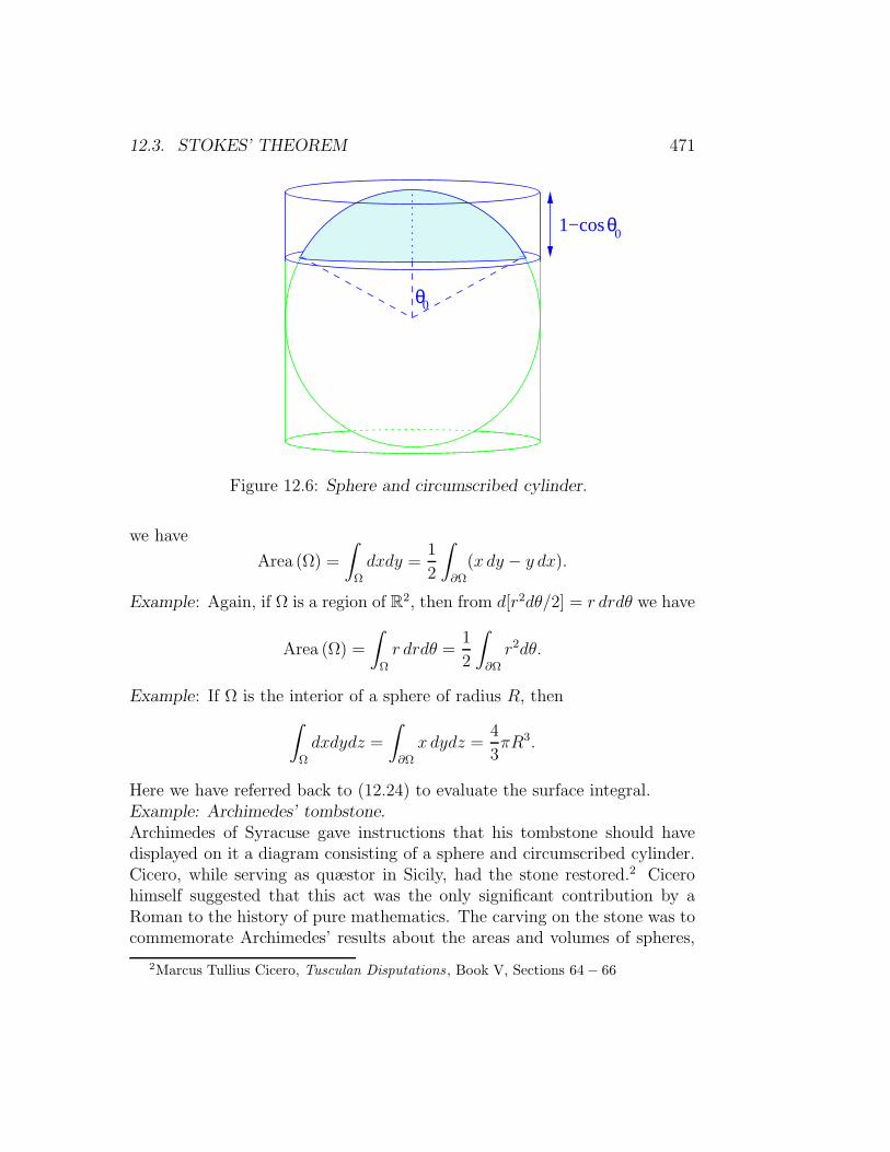
12.3. STOKES’ THEOREM 471
1−cos 0
0θ
θ
Figure 12.6: Sphere and circumscribed cylinder.
we have
Area (Ω) =
∫
Ω
dxdy =1
2
∫
∂Ω
(x dy − y dx).
Example: Again, if Ω is a region of R2, then from d[r2dθ/2] = r drdθ we have
Area (Ω) =
∫
Ω
r drdθ =1
2
∫
∂Ω
r2dθ.
Example: If Ω is the interior of a sphere of radius R, then
∫
Ω
dxdydz =
∫
∂Ω
x dydz =4
3πR3.
Here we have referred back to (12.24) to evaluate the surface integral.Example: Archimedes’ tombstone.Archimedes of Syracuse gave instructions that his tombstone should havedisplayed on it a diagram consisting of a sphere and circumscribed cylinder.Cicero, while serving as quæstor in Sicily, had the stone restored.2 Cicerohimself suggested that this act was the only significant contribution by aRoman to the history of pure mathematics. The carving on the stone was tocommemorate Archimedes’ results about the areas and volumes of spheres,
2Marcus Tullius Cicero, Tusculan Disputations , Book V, Sections 64− 66

472 CHAPTER 12. INTEGRATION ON MANIFOLDS
including the one illustrated in figure 12.6, that the area of the spherical capcut off by slicing through the cylinder is equal to the area cut off on thecylinder.
We can understand this result via Stokes’ theorem: If the two-sphere S2
is parametrized by spherical polar co-ordinates θ, φ, and Ω is a region on thesphere, then
Area (Ω) =
∫
Ω
sin θdθdφ =
∫
∂Ω
(1− cos θ)dφ,
and applying this to the figure, where the cap is defined by θ < θ0 gives
Area (cap) = 2π(1− cos θ0)
which is indeed the area cut off on the cylinder.
Exercise 12.2: The sphere Sn can be thought of as the locus of points in Rn+1
obeying∑n+1
i=1 (xi)2 = 1. Use its invariance under orthogonal transformations
to show that the element of surface “volume” of the n-sphere can be writtenas
d(Volume on Sn) =1
n!ǫα1α2...αn+1
xα1 dxα2 . . . dxαn+1 .
Use Stokes’ theorem to relate the integral of this form over the surface of thesphere to the volume of the solid unit sphere. Confirm that we get the correctproportionality between the volume of the solid unit sphere and the volumeor area of its surface.
12.4 Applications
We now know how to integrate forms. What sort of forms should we seekto integrate? For a physicist working with a classical or quantum field, aplentiful supply of intesting forms is obtained by using the field to pull backgeometric objects.
12.4.1 Pull-backs and Push-forwards
If we have a map φ from a manifoldM to another manifold N , and we choosea point x ∈ M , we can push forward a vector from TMx to TNφ(x), in theobvious way (map head-to-head and tail-to-tail). This map is denoted byφ∗ : TMx → TNφ(x).
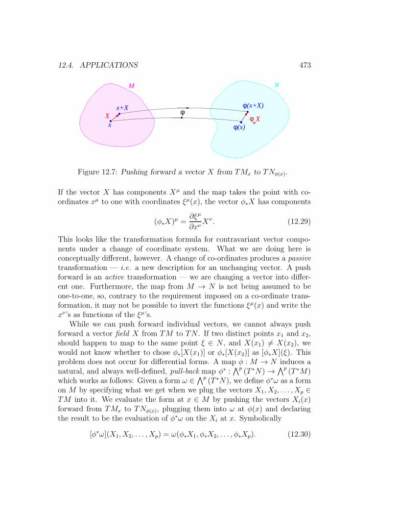
12.4. APPLICATIONS 473
x
x+XX Xφ
*φ(x)
φ(x+X)
M N
φ
Figure 12.7: Pushing forward a vector X from TMx to TNφ(x).
If the vector X has components Xµ and the map takes the point with co-ordinates xµ to one with coordinates ξµ(x), the vector φ∗X has components
(φ∗X)µ =∂ξµ
∂xνXν . (12.29)
This looks like the transformation formula for contravariant vector compo-nents under a change of coordinate system. What we are doing here isconceptually different, however. A change of co-ordinates produces a passivetransformation — i.e. a new description for an unchanging vector. A pushforward is an active transformation — we are changing a vector into differ-ent one. Furthermore, the map from M → N is not being assumed to beone-to-one, so, contrary to the requirement imposed on a co-ordinate trans-formation, it may not be possible to invert the functions ξµ(x) and write thexν ’s as functions of the ξµ’s.
While we can push forward individual vectors, we cannot always pushforward a vector field X from TM to TN . If two distinct points x1 and x2,should happen to map to the same point ξ ∈ N , and X(x1) 6= X(x2), wewould not know whether to chose φ∗[X(x1)] or φ∗[X(x2)] as [φ∗X ](ξ). Thisproblem does not occur for differential forms. A map φ : M → N induces anatural, and always well-defined, pull-back map φ∗ :
∧p (T ∗N)→ ∧p (T ∗M)which works as follows: Given a form ω ∈ ∧p (T ∗N), we define φ∗ω as a formon M by specifying what we get when we plug the vectors X1, X2, . . . , Xp ∈TM into it. We evaluate the form at x ∈ M by pushing the vectors Xi(x)forward from TMx to TNφ(x), plugging them into ω at φ(x) and declaringthe result to be the evaluation of φ∗ω on the Xi at x. Symbolically
[φ∗ω](X1, X2, . . . , Xp) = ω(φ∗X1, φ∗X2, . . . , φ∗Xp). (12.30)

474 CHAPTER 12. INTEGRATION ON MANIFOLDS
This may seem rather abstract, but the idea is in practice quite simple:If the map takes x ∈M → ξ(x) ∈ N , and if
ω =1
p!ωi1...ip(ξ)dξ
i1 . . . dξip, (12.31)
then
φ∗ω =1
p!ωi1i2...ip[ξ(x)]dξ
i1(x)dξi2(x) · · · dξip(x)
=1
p!ωi1i2...ip[ξ(x)]
∂ξi1
∂xµ1∂ξi2
∂xµ2· · · ∂ξ
ip
∂xµ1dxµp · · ·dxµp . (12.32)
Computationally, the process of pulling back a form is so transparent thatit easy to confuse it with a simple change of variable. That it is not the sameoperation will become clear in the next few sections where we consider mapsthat are many-to-one.
Exercise 12.3: Show that the operation of taking an exterior derivative com-mutes with a pull back:
d [φ∗ω] = φ∗(dω).
Exercise 12.4: If the map φ :M → N is invertible then we may push forwarda vector field X on M to get a vector field φ∗X on N . Show that
LX [φ∗ω] = φ∗ [Lφ∗Xω] .
Exercise 12.5: Again assume that φ : M → N is invertible. By using the co-ordinate expressions for the Lie bracket along with the effect of a push-forward,show that if X, Y are vector fields on TM then
φ∗([X,Y ]) = [φ∗X,φ∗Y ],
as vector fields on TN .
12.4.2 Spin textures
As an application of pull-backs we consider some of the topological aspectsof spin textures which are fields of unit vectors n, or “spins”, in two or threedimensions.

12.4. APPLICATIONS 475
Consider a smooth map ϕ : R2 → S2 that assigns x 7→ n(x), where n is athree-dimensional unit vector whose tip defines a point on the 2-sphere S2.A physical example of such an n(x) would be the local direction of the spinpolarization in a ferromagnetically-coupled two-dimensional electron gas.
In terms of n, the area 2-form on the 2-sphere becomes
Ω =1
2n · (dn× dn) ≡ 1
2ǫijkn
idnjdnk. (12.33)
The ϕ map pulls this area-form back to
F ≡ ϕ∗Ω =1
2(ǫijkn
i∂µnj∂νn
k)dxµdxν = (ǫijkni∂1n
j∂2nk) dx1dx2 (12.34)
which is a differential form in R2. We will call it the topological chargedensity . It measures the area on the two-sphere swept out by the n vectorsas we explore a square in R2 of side dx1 by dx2.
Suppose now that the n tends the same unit vector n(∞) at large distancein all directions. This allows us to think of “infinity” as a single point, andthe assignment ϕ : x 7→ n(x) as a map from S2 to S2. Such maps arecharacterized topologically by their “topological charge,” or winding numberN which counts the number of times the image of the originating x spherewraps round the target n-sphere. A mathematician would call this numberthe Brouwer degree of the map ϕ. It is intuitively plausible that a continuousmap from a sphere to itself will wrap a whole number of times, and so weexpect
N =1
4π
∫
R2
ǫijkn
i∂1nj∂2n
kdx1dx2, (12.35)
to be an integer. We will soon show that this is indeed so, but first we willdemonstrate that N is a topological invariant .
In two dimensions the form F = ϕ∗Ω is automatically closed becausethe exterior derivative of any two-form is zero — there being no three-formsin two dimensions. Even if we consider a field n(x1, . . . , xm) in m > 2dimensions, however, we still have dF = 0. This is because
dF =1
2ǫijk∂σn
i∂µnj∂νn
kdxσdxµdxν . (12.36)
If we plug infinitesimal vectors into the dxµ to get their components δxµ,we have to evaluate the triple-product of three vectors δni = ∂µn
iδxµ, each

476 CHAPTER 12. INTEGRATION ON MANIFOLDS
of which is tangent to the two-sphere. But the tangent space of S2 is two-dimensional, so any three tangent vectors t1, t2, t3, are linearly dependentand their triple-product t1 · (t2 × t3) is therefore zero.
Although it is closed, F = ϕ∗Ω will not generally be the d of a globallydefined one-form. Suppose, however, that we vary the map so that n(x) →n(x) + δn(x). The corresponding change in the topological charge density is
δF = ϕ∗[n · (d(δn)× dn)], (12.37)
and this variation can be written as a total derivative:
δF = dϕ∗[n · (δn× dn)] ≡ dǫijkniδnj∂µnkdxµ. (12.38)
In these manipulations we have used δn · (dn×dn) = dn · (δn×dn) = 0, thetriple-products being zero for the linear-dependence reason adduced earlier.From Stokes’ theorem, we have
δN =
∫
S2
δF =
∫
∂S2
ǫijkniδnj∂µn
kdxµ. (12.39)
Because the sphere has no boundary, i.e. ∂S2 = ∅, the last integral vanishes,so we conclude that δN = 0 under any smooth deformation of the mapn(x). This is what we mean when we say that N is a topological invariant.Equivalently, on R2, with n constant at infinity, we have
δN =
∫
R2
δF =
∫
Γ
ǫijkniδnj∂µn
kdxµ, (12.40)
where Γ is a curve surrounding the origin at large distance. Again δN = 0,this time because ∂µn
k = 0 everywhere on Γ.In some physical applications, the field n winds in localized regions called
skyrmions . These knots in the spin field behave very much as elementaryparticles, retaining their identity as they move through the system. Thewinding number counts how many skyrmions (minus the number of anti-skyrmions, which wind with opposite orientation) there are. To constructa smooth multi-skyrmion map ϕ : R2 → S2 with positive winding numberN , take a set of N + 1 complex numbers λ, a1, . . . , aN and another set of Ncomplex numbers b1, . . . , bN such that no b coincides with any a. Then put
eiφ tanθ
2= λ
(z − a1) . . . (z − aN )(z − b1) . . . (z − bN )
(12.41)

12.4. APPLICATIONS 477
where z = x1 + ix2, and θ and φ are spherical polar co-ordinates specifyingthe direction n at the point (x1, x2). At the points z = ai the vector n pointsstraight up, and at the points z = bi it points straight down. You will show inexercise 12.12 that this particular n-field configuration minimizes the energyfunctional
E[n] =1
2
∫(∂1n · ∂1n+ ∂2n · ∂2n) dx1dx2
=1
2
∫ (|∇n1|2 + |∇n2|2 + |∇n3|2
)dx1dx2 (12.42)
for the given winding number N . In the next section we will explain thegeometric origin of the mysterious combination eiφ tan θ/2.
12.4.3 The Hopf Map
You may recall that in section 10.2.3 we defined complex projective spaceCP n to be the set of rays in a complex n + 1 dimensional vector space.A ray is an equivalence classes of vectors [ζ1, ζ2, . . . , ζn+1], where the ζi arenot all zero, and where we do not distinguish between [ζ1, ζ2, . . . , ζn+1] and[λζ1, λζ2, . . . , λζn+1] for non-zero complex λ. The space of rays is a 2n-dimensional real manifold: in a region where ζn+1 does not vanish, we cantake as co-ordinates the real numbers ξ1, . . . , ξn, η1, . . . , ηn where
ξ1 + iη1 =ζ1ζn+1
, ξ2 + iη2 =ζ2ζn+1
, . . . , ξn + iηn =ζnζn+1
. (12.43)
Similar co-ordinate charts can be constructed in the regions where other ζiare non-zero. Every point in CP n lies in at least one of these co-ordinatecharts, and the co-ordinate transformation rules for going from one chart toanother are smooth.
The simplest complex projective space, CP 1, is the real two-sphere S2 indisguise. This rather non-obvious fact is revealed by the use of a stereographicmap to make the equivalence class [ζ1, ζ2] ∈ CP 1 correspond to a point n onthe sphere. When ζ1 is non zero, the class [ζ1, ζ2] is uniquely determined bythe ratio ζ2/ζ1 = |ζ2/ζ1|eiφ, which we plot on the complex plane. We thinkof this copy of C as being the x, y plane in R3. We then draw a straight lineconnecting the plotted point to the south pole of a unit sphere circumscribedabout the origin in R3. The point where this line (continued, if necessary)intersects the sphere is the tip of the unit vector n.

478 CHAPTER 12. INTEGRATION ON MANIFOLDS
θ
θ/2
S2
n
1ζ /ζ
2 1=ζ
N
S
z
y
n ζ
x
S
N
Figure 12.8: Two views of the stereographic map between the two-sphereand the complex plane. The point ζ = ζ2/ζ1 ∈ C corresponds to the unitvector n ∈ S2.
If ζ2 were zero, n would end up at the north pole, where the R3 co-ordinatez takes the value z = 1. If ζ1 goes to zero with ζ2 fixed, n moves smoothly tothe south pole z = −1. We therefore extend the definition of our map to thecase ζ1 = 0 by making the equivalence class [0, ζ2] correspond to the southpole. We can find an explicit formula for this map. Figure 12.8 shows thatζ2/ζ1 = eiφ tan θ/2, and this relation suggests the use of the “t”-substitutionformulæ:
sin θ =2t
1 + t2, cos θ =
1− t21 + t2
, (12.44)
where t = tan θ/2. Since the x, y, z components of n are given by
n1 = sin θ cosφ,
n2 = sin θ sinφ,
n3 = cos θ, (12.45)
we find that
n1 + in2 =2(ζ2/ζ1)
1 + |ζ2/ζ1|2, n3 =
1− |ζ2/ζ1|21 + |ζ2/ζ1|2
. (12.46)
We can multiply through by |ζ1|2 = ζ1ζ1, and so write this correspondencein a more symmetrical manner:
n1 =ζ1ζ2 + ζ2ζ1|ζ1|2 + |ζ2|2
,

12.4. APPLICATIONS 479
n2 =1
i
(ζ1ζ2 − ζ2ζ1|ζ1|2 + |ζ2|2
),
n3 =|ζ1|2 − |ζ2|2|ζ1|2 + |ζ2|2
. (12.47)
This last form can be conveniently expressed in terms of the Pauli sigmamatrices
σ1 =
(0 11 0
), σ2 =
(0 −ii 0
), σ3 =
(1 00 −1
). (12.48)
as
n1 = (z1, z2)
(0 11 0
)(z1z2
),
n2 = (z1, z2)
(0 −ii 0
)(z1z2
),
n3 = (z1, z2)
(1 00 −1
)(z1z2
), (12.49)
where (z1z2
)=
1√|ζ1|2 + |ζ2|2
(ζ1ζ2
)(12.50)
is a normalized 2-vector, which we think of as a spinor .The correspondence CP 1 ≃ S2 now has a quantum-mechanical interpre-
tation: Any unit three-vector n can be obtained as the expectation valueof the σ matrices in a normalized spinor state. Conversely, any normalizedspinor ψ = (z1, z2)
T gives rise to a unit vector via
ni = ψ†σiψ. (12.51)
Now, since
1 = |z1|2 + |z2|2, (12.52)
the normalized spinor can be thought of as defining a point in S3. Thismeans that the one-to-one correspondence [z1, z2] ↔ n also gives rise to amap from S3 → S2. This is called the Hopf map:
Hopf : S3 → S2. (12.53)

480 CHAPTER 12. INTEGRATION ON MANIFOLDS
The dimension reduces from three to two, so the Hopf map cannot be one-to-one. Even after we have normalized [ζ1, ζ2], we are still left with a choice ofoverall phase. Both (z1, z2) and (z1e
iθ, z2eiθ), although distinct points in S3,
correspond to the same point in CP 1, and hence in S2. The inverse image ofa point in S2 is a geodesic circle in S3. Later, we will show that any two suchgeodesic circles are linked, and this makes the Hopf map topologically non-trivial, in that it cannot be continuously deformed to a constant map—i.e. toa map that takes all of S3 to a single point in S2.
Exercise 12.6: We have seen that the stereographic map relates the point withspherical polar co-ordinates θ, φ to the complex number
ζ = eiφ tan θ/2.
We can therefore set ζ = ξ + iη and take ξ, η as stereographic co-ordinates onthe sphere. Show that in these co-ordinates the sphere metric is given by
g( , ) ≡ dθ ⊗ dθ + sin2θ dφ⊗ dφ=
2
(1 + |ζ|2)2 (dζ ⊗ dζ + dζ ⊗ dζ)
=4
(1 + ξ2 + |η|2)2 (dξ ⊗ dξ + dη ⊗ dη),
and that the area 2-form becomes
Ω ≡ sin θ dθ ∧ dφ=
2i
(1 + |ζ|2)2 dζ ∧ dζ
=4
(1 + ξ2 + η2)2dξ ∧ dη. (12.54)
12.4.4 Homotopy and the Hopf map
We can use the Hopf map to factor the map ϕ : x 7→ n(x) via the three-sphere by specifying the spinor ψ at each point, instead of the vector n, andso mapping indirectly
ϕ : R2 ψ→ S3 Hopf→ S2.
It might seem that for a given spin-field n(x) we can choose the overall phaseof ψ(x) ≡ (z1(x), z2(x))
T as we like, however, if we demand that the zi’sbe continuous functions of x then there is a rather non-obvious topological

12.4. APPLICATIONS 481
restriction which has important physical consequences. To see how this comesabout, we first express the winding number in terms of the zi. We find (aftera page or two of algebra) that
F = (ǫijkni∂1n
j∂2nk) dx1dx2 =
2
i
2∑
i=1
(∂1zi∂2zi − ∂2zi∂1zi) dx1dx2, (12.55)
and so the topological charge N is given by
N =1
2πi
∫ 2∑
i=1
(∂1zi∂2zi − ∂2zi∂1zi) dx1dx2. (12.56)
Now, when written in terms of the zi variables, the form F becomes a totalderivative:
F =2
i
2∑
i=1
(∂1zi∂2zi − ∂2zi∂1zi) dx1dx2
= d
1
i
2∑
i=1
(zi∂µzi − (∂µzi)zi) dxµ
. (12.57)
Furthermore, because n is fixed at large distance, we have (z1, z2) = eiθ(c1, c2)near infinity, where c1, c2 are constants with |c1|2 + |c2|2 = 1. Thus, nearinfinity,
1
2i
2∑
i=1
(zi∂µzi − (∂µzi)zi)→ (|c1|2 + |c2|2)dθ = dθ. (12.58)
We combine this observation with Stokes’ theorem to obtain
N =1
2πi
∫
Γ
1
2
2∑
i=1
(zi∂µzi − (∂µzi)zi) dxµ =
1
2π
∫
Γ
dθ. (12.59)
Here, as in the previous section, Γ is a curve surrounding the origin at largedistance. Now
∫dθ is the total change in θ as we circle the boundary. While
the phase eiθ has to return to its original value after a round trip, the angleθ can increase by an integer multiple of 2π. The winding number
∮dθ/2π
can therefore be non-zero, but must be an integer.
482 CHAPTER 12. INTEGRATION ON MANIFOLDS
We have uncovered the rather surprising fact that the topological chargeof the map ϕ : S2 → S2 is equal to the winding number of the phase angleθ at infinity. This is the topological restriction referred to in the preced-ing paragraph. As a byproduct, we have confirmed our conjecture that thetopological charge N is an integer. The existence of this integer invariantshows that the smooth maps ϕ : S2 → S2 fall into distinct homotopy classeslabelled by N . Maps with different values of N cannot be continuously de-formed into one another, and, while we have not shown that it is so, twomaps with the same value of N can be deformed into each other.
Maps that can be continuously deformed one into the other are said tobe homotopic. The set of homotopy classes of the maps of the n-sphere intoa manifold M is denoted by πn(M). In the present case M = S2. We aretherefore claiming that
π2(S2) = Z, (12.60)
where we are identifying the homotopy class with its winding number N ∈ Z.
12.4.5 The Hopf index
We have so far discussed maps from S2 to S2. It is perhaps not too surprisingthat such maps are classified by a winding number. What is rather moresurprising is that maps ϕ : S3 → S2 also have an associated topologicalnumber. If we continue to assume that n tends to a constant vector atinfinity so that we can think of R3∪∞ as being S3, this number will labelthe homotopy classes π3(S
2) of fields of unit vectors n in three dimensions.We will think of the third dimension as being time. In this situation aninteresting set of n fields to consider are the n(x, t) corresponding movingskyrmions. The world lines of these skyrmions will be tubes outside of whichn is constant, and such that on any slice through the tube, n will cover thetarget n-sphere once.
To motivate the formula we will find for the topological number, we beginwith a problem from magnetostatics. Suppose we are given a cable originallymade up of a bundle of many parallel wires. The cable is then twisted Ntimes about its axis and bent into a closed loop, the end of each individualwire being attached to its begining to make a continuous circuit. A current Iflows in the cable in such a manner that each individual wire carries only aninfinitesimal part δIi of the total. The sense of the current is such that as weflow with it around the cable each wire wraps N times anticlockwise about

12.4. APPLICATIONS 483
I
Figure 12.9: A twisted cable with N = 5.
all the others. The current produces a magnetic field B. Can we determinethe integer twisting number N knowing only this B field?The answer is yes . We use Ampere’s law in integral form,
∮
Γ
B · dr = (current encircled by Γ). (12.61)
We also observe that the current density ∇ × B = J at a point is directedalong the tangent to the wire passing through that point. We thereforeintegrate along each individual wire as it encircles the others, and sum overthe wires to find
NI2 =∑
wires i
δIi
∮B · dri =
∫B · J d3x =
∫B · (∇×B) d3x. (12.62)
We now apply this insight to our three-dimensional field of unit vectors n(x).The quantity playing the role of the current density J is the topological cur-rent
Jσ =1
2ǫσµνǫijkn
i∂µnj∂νn
k. (12.63)
Observe that div J = 0. This is simply another way of saying that the 2-formF = ϕ∗Ω is closed.

484 CHAPTER 12. INTEGRATION ON MANIFOLDS
The flux of J through a surface S is
I =
∫
S
J · dS =
∫
S
F (12.64)
and this is the area of the spherical surface covered by the n’s. A skyrmion,for example, has total topological current I = 4π, the total surface area ofthe 2-sphere. The skyrmion world-line will play the role of the cable, andthe inverse images in R3 of points on S2 correspond to the individual wires.
If form language, the field corresponding to B can be any one-form Asuch that dA = F . Thus
NHopf =1
I2
∫
R3
B · J d3x =1
16π2
∫
R3
AF (12.65)
will be an integer. This integer is the Hopf linking number, or Hopf index,and counts the number of times the skyrmion twists before it bites its tail toform a closed-loop world-line.
There is another way of obtaining this formula, and of understanding thenumber 16π2. We observe that the two-form F and the one-form A are thepull-back from S3 to R3 along ψ of the forms
F =1
i
2∑
i=1
(dzidzi − dzidzi) ,
A =1
i
2∑
i=1
(zidzi − zidzi) , (12.66)
respectively. If we substitute z1,2 = ξ1,2 + iη1,2, we find that
AF = 8(ξ1dη1dξ2dη2 − η1dξ1dξ2dη2 + ξ2dη2dξ1dη1 − η2dξ2dξ1dη1). (12.67)
We know from exercise 12.2 that this expression is eight times the volume3-form on the three-sphere. Now the total volume of the unit three-sphere is2π2, and so, from our factored map x 7→ ψ 7→ n we have that
NHopf =1
16π2
∫
R3
ψ∗(AF ) = 1
2π2
∫
R3
ψ∗d(Volume on S3) (12.68)
is the number of times the normalized spinor ψ(x) covers S3 as x covers R3.For the Hopf map itself, this number is unity, and so the loop in S3 that

12.4. APPLICATIONS 485
is the inverse image of a point in S2 will twist once around any other suchinverse image loop.
We have now established that
π3(S2) = Z. (12.69)
This result, implying that there are many maps from the three-sphere tothe two-sphere that are not smoothly deformable to a constant map, was angreat surprise when Hopf discovered it.
One of the principal physics consequences of the existence of the Hopfindex is that “quantum lump” quasi-particles such as the skyrmion canbe fermions, even though they are described by commuting (and thereforebosonic) fields.
To understand how this can be, we first explain that the collection ofhomotopy classes πn(M) is not just a set . It has the additional structureof being a group: we can compose two homotopy classes to get a third, thecomposition is associative, and each homotopy class has an inverse. To definethe group composition law, we think of Sn as the interior of an n-dimensionalcube with the map f : Sn → M taking a fixed value m0 ∈ M at all pointson the boundary of the cube. The boundary can then be considered to be asingle point on Sn. We then take one of the n dimensions as being “time” andplace two cubes and their maps f1, f2 into contact, with f1 being “earlier”and f2 being “later.” We thus get a continuous map from a bigger box intoM . The homotopy class of this map, after we relax the condition that themap takes the value m0 on the common boundary, defines the composition[f2] [f1] of the two homotopy classes corresponding to f1 and f2. Thecomposition may be shown to be independent of the choice of representativefunctions in the two classes. The inverse of a homotopy class [f ] is obtainedby reversing the direction of “time” for each of the maps in the class. Thisgroup structure appears to depend on the fixed point m0. As long as Mis arcwise connected, however, the groups obtained from different m0’s areisomorphic, or equivalent. In the case of π2(S
2) = Z and π3(S2) = Z, the
composition law is simply the addition of the integers N ∈ Z that label theclasses. A useful exposition of homotopy theory for physicists is to be foundin a review article by David Mermin.3
When we quantize using Feynman’s “sum over histories” path integral,we have the option of multiplying the contributions of histories f that are
3N. D. Mermin, “The topological theory of defects in ordered media.” Rev. Mod. Phys.51 (1979) 591.

486 CHAPTER 12. INTEGRATION ON MANIFOLDS
not deformable into one another by distinct phase factors expiφ([f ]). Thechoice of phases must, however, be compatible with the composition of histo-ries by concatenating one after the other – the same operation as composinghomotopy classes. This means that the product expiφ([f1])) expiφ([f2])of the phase factors for two possible histories must be the phase factorexpiφ([f2] [f1]) assigned to the composition of their homotopy classes.If our quantum system consists of spins n in two space and one time dimen-sion we can consistently assign a phase factor exp(iπNHopf) to a history. Therotation of a single skyrmion twists the world-line cable through 2π and somakes NHopf = 1. The rotation therefore causes the wavefunction to changesign. We will show in the next section, that a history where two particleschange places can be continuously deformed into a history where they do notinterchange, but instead one of them is twisted through 2π. The wavefunc-tion of a pair of skyrmions therefore changes sign when they are interchanged.This means that the quantized skyrmion is a fermion.
12.4.6 Twist and Writhe
Consider two oriented non-intersecting closed curves γ1 and γ2. Imagine thatγ2 carries a unit current in the direction of its orientation and so gives riseto a magnetic field. Ampere’s law then tells us that the number of times γ1encircles γ2 is
Lk(γ1, γ2) =
∮
γ1
B(r1) · dr1
=1
4π
∮
γ1
∮
γ2
(r1 − r2) · (dr1 × dr2)|r1 − r2|3
. (12.70)
Here the second expression follows from the first by an application of theBiot-Savart law to compute the B field due the current. This expression alsoshows that Lk(γ1, γ2), which is called the Gauss linking number , is symmetricunder the interchange γ1 ↔ γ2 of the two curves. It changes sign, however,if one of the curves changes orientation, or if the pair of curves is reflectedin a mirror.
We can relate the Gauss linking number to the Brouwer degree of a map.Introduce parameters t1, t2 with 0 < t1, t2 ≤ 1 to label points on the twocurves. The curves are closed, so r1(0) = r1(1), and similarly for r2. Let us

12.4. APPLICATIONS 487
also define a unit vector
n(t1, t2) =r1(t1)− r2(t2)
|r1(t1)− r2(t2)|. (12.71)
Then
Lk(γ1, γ2) =1
4π
∮
γ1
∮
γ2
r1(t1)− r2(t2)
|r1(t1)− r2(t2)|3·(∂r1∂t1× ∂r2∂t2
)dt1dt2
= − 1
4π
∫
T 2
n ·(∂n
∂t1× ∂n
∂t2
)dt1dt2. (12.72)
is seen to be (minus) the winding number of the map
n : [0, 1]× [0, 1]→ S2 (12.73)
of the 2-torus into the sphere. Our previous results on maps into the 2-spheretherefore confirm our Ampere-law intuition that Lk(γ1, γ2) is an integer. Thelinking number is also topological invariant, being unchanged under any de-formation of the curves that does not cause one to pass through the other.
An important application of these ideas occurs in biology, where thecurves are the two complementary strands of a closed loop of DNA. We canthink of two such parallel curves as forming the edges of a ribbon γ1, γ2 ofwidth ǫ. Let use denote by γ the curve r(t) running along the axis of theribbon midway between γ1 and γ2. The unit tangent to γ at the point r(t) is
t(t) =r(t)
|r(t)| , (12.74)
where, as usual, the dots denote differentiation with respect to t. We alsointroduce a unit vector u(t) that is perpendicular to t(t) and lies in theribbon, pointing from r1(t) to r2(t).
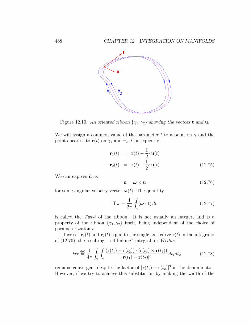
488 CHAPTER 12. INTEGRATION ON MANIFOLDS
t
u
γ γ1 2
Figure 12.10: An oriented ribbon γ1, γ2 showing the vectors t and u.
We will assign a common value of the parameter t to a point on γ and thepoints nearest to r(t) on γ1 and γ2. Consequently
r1(t) = r(t)− 1
2ǫu(t)
r2(t) = r(t) +1
2ǫu(t) (12.75)
We can express u asu = ω × u (12.76)
for some angular-velocity vector ω(t). The quantity
Tw =1
2π
∮
γ
(ω · t) dt (12.77)
is called the Twist of the ribbon. It is not usually an integer, and is aproperty of the ribbon γ1, γ2 itself, being independent of the choice ofparameterization t.
If we set r1(t) and r2(t) equal to the single axis curve r(t) in the integrandof (12.70), the resulting “self-linking” integral, or Writhe,
Wrdef=
1
4π
∮
γ
∮
γ
(r(t1)− r(t2)) · (r(t1)× r(t2))
|r(t1)− r(t2)|3dt1dt2. (12.78)
remains convergent despite the factor of |r(t1)− r(t2)|3 in the denominator.However, if we try to achieve this substitution by making the width of the

12.4. APPLICATIONS 489
ribbon ǫ tend to zero, we find that the vector n(t1, t2) abruptly reverses itsdirection as t1 passes t2. In the limit of infinitesimal width this violent motionprovides a delta-function contribution
−(ω · t)δ(t1 − t2) dt1 ∧ dt2 (12.79)
to the 2-sphere area swept out by n, and this contribution is invisible to theWrithe integral. The Writhe is a property only of the overall shape of theaxis curve γ, and is independent both of the ribbon that contains it, and ofthe choice of parameterization. The linking number, on the other hand, isindependent of ǫ, so the ǫ→ 0 limit of the linking-number integral is not theintegral of the ǫ→ 0 limit of its integrand. Instead we have
Lk(γ1, γ2) =1
2π
∮
γ
(ω · t) dt+ 1
4π
∮
γ
∮
γ
(r(t1)− r(t2)) · (r(t1)× r(t2))
|r(t1)− r(t2)|3dt1dt2
(12.80)
This formulaLk = Tw +Wr (12.81)
is known as the Calugareanu-White-Fuller relation, and is the basis for theclaim, made in the previous section, that the worldline of an extended particlewith an exchange (Wr = ±1) can be deformed into a worldline with a 2πrotation (Tw = ±1) without changing the topologically invariant linkingnumber.
1
t2
t110
t−t
Γ Γt t( )
−t t( )
Figure 12.11: Cutting and reassembling the domain of integration in (12.83).
By setting
n(t1, t2) =r(t1)− r(t2)
|r(t1)− r(t2)|. (12.82)

490 CHAPTER 12. INTEGRATION ON MANIFOLDS
we can express the Writhe as
Wr = − 1
4π
∫
T 2
n ·(∂n
∂t1× ∂n
∂t2
)dt1dt2, (12.83)
but we must take care to recognize that this new n(t1, t2) is discontinuousacross the line t = t1 = t2. It is equal to t(t) for t1 infinitesimally largerthan t2, and equal to −t(t) when t1 is infinitesimally smaller than t2. Bycutting the square domain of integration and reassembling it into a rhom-boid, as shown in figure 12.11, we obtain a continuous integrand and seethat the Writhe is (minus) the 2-sphere area (counted with multiplicies anddivided by 4π) of a region whose boundary is composed of two curves Γ, thetangent indicatrix , or tantrix , on which n = t(t), and its oppositely orientedantipodal counterpart Γ′ on which n = −t(t).
The 2-sphere area Ω(Γ) bounded by Γ is only determined by Γ up to theaddition of integer multiples of 4π. Taking note that the “wrong” orientationof the boundary Γ (see figure 12.11 again) compensates for the minus signbefore the integral in (12.83), we have
4πWr = 2Ω(Γ) + 4πn. (12.84)
Thus,
Wr =1
2πΩ(Γ), mod 1. (12.85)
We can do better than (12.85) once we realize that by allowing crossings wecan continuously deform any closed curve into a perfect circle. Each self-crossing causes Lk and Wr (but not Tw which, being a local functional, doesnot care about crossings) to jump by ±2. For a perfect circle Wr = 0 whilstΩ = 2π. We therefore have an improved estimate of the additive integer thatis left undetermined by Γ, and from it we obtain
Wr = 1 +1
2πΩ(Γ), mod 2. (12.86)
This result is due to Brock Fuller.4
We can use our ribbon language to describe conformational transitions inlong molecules. The elastic energy of a closed rod (or DNA molecule) can beapproximated by
E =
∫
γ
1
2α(ω · t)2 + 1
2βκ2ds (12.87)
4F. Brock Fuller, Proc. Natl. Acad. Sci. USA, 75 (1978) 3557 - 61.
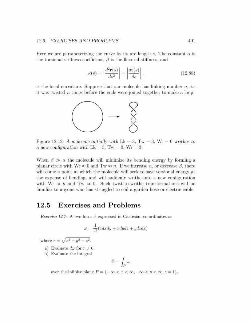
12.5. EXERCISES AND PROBLEMS 491
Here we are parameterizing the curve by its arc-length s. The constant α isthe torsional stiffness coefficient, β is the flexural stiffness, and
κ(s) =
∣∣∣∣d2r(s)
ds2
∣∣∣∣ =∣∣∣∣dt(s)
ds
∣∣∣∣ , (12.88)
is the local curvature. Suppose that our molecule has linking number n, i.eit was twisted n times before the ends were joined together to make a loop.
Figure 12.12: A molecule initially with Lk = 3, Tw = 3, Wr = 0 writhes toa new configuration with Lk = 3, Tw = 0, Wr = 3.
When β ≫ α the molecule will minimize its bending energy by forming aplanar circle with Wr ≈ 0 and Tw ≈ n. If we increase α, or decrease β, therewill come a point at which the molecule will seek to save torsional energy atthe expense of bending, and will suddenly writhe into a new configurationwith Wr ≈ n and Tw ≈ 0. Such twist-to-writhe transformations will befamiliar to anyone who has struggled to coil a garden hose or electric cable.
12.5 Exercises and Problems
Exercise 12.7: A two-form is expressed in Cartesian co-ordinates as
ω =1
r3(zdxdy + xdydz + ydzdx)
where r =√x2 + y2 + z2.
a) Evaluate dω for r 6= 0.b) Evaluate the integral
Φ =
∫
Pω,
over the infinite plane P = −∞ < x <∞,−∞ < y <∞, z = 1.

492 CHAPTER 12. INTEGRATION ON MANIFOLDS
c) A sphere is embedded into R3 by the map ϕ, which takes the point(θ, φ) ∈ S2 to the point (x, y, z) ∈ R3, where
x = R cosφ sin θ,
y = R sinφ sin θ,
z = R cos θ.
Pull back ω and find the 2-form ϕ∗ω on the sphere. (Hint: The formϕ∗ω is both familiar and simple. If you end up with an intractable messof trigonometric functions, you have made an algebraic error.)
d) By exploiting the result of part c), or otherwise, evaluate the integral
Φ =
∫
S2(R)ω
where S2(R) is the surface of a two-sphere of radius R centered at theorigin.
The following four exercises all explore the same geometric facts relating toStokes’ theorem and the area 2-form of a sphere, but in different physicalsettings.
Exercise 12.8: A flywheel of moment of inertia I can rotate without frictionabout an axle whose direction is specified by a unit vector n. The flywheel andaxle are initially stationary. The direction n of the axle is made to describe asimple closed curve γ = ∂Ω on the unit sphere, and is then left stationary.
γ
Ωn
Figure 12.13: Flywheel

12.5. EXERCISES AND PROBLEMS 493
Show that once the axle has returned to rest in its initial direction, the flywheelhas also returned to rest, but has rotated through an angle θ = Area(Ω) whencompared with its initial orientation. The area of Ω is to be counted as positiveif the path γ surrounds it in a clockwise sense, and negative otherwise. Observethat the path γ bounds two regions with opposite orientations. Taking intoaccount the fact that we cannot define the rotation angle at intermediatesteps, show that the area of either region can be used to compute θ, theresults being physically indistinguishable. (Hint: Show that the componentLZ = I(ψ + φ cos θ) of the flywheel’s angular momentum along the axle is aconstant of the motion.)
Exercise 12.9: A ball of unit radius rolls without slipping on a table. Theball moves in such a way that the point in contact with table describes aclosed path γ = ∂Ω on the ball . (The corresponding path on the table will notnecessarily be closed.) Show that the final orientation of the ball will be suchthat it has rotated, when compared with its initial orientation, through anangle φ = Area(Ω) about a vertical axis through its center. As in the previousproblem, the area is counted positive if γ encircles Ω in an anti-clockwise sense.(Hint: recall the no-slip rolling condition φ+ ψ cos θ = 0 from (11.29).)
Exercise 12.10: Let a curve in R3 be parameterized by its arc length s as r(s).Then the unit tangent to the curve is given by
t(s) = rdef=
dr
ds.
The principal normal n(s) and the binormal b(s) to the curve are defined bythe requirement that t = κn with the curvature κ(s) positive, and that t, nand b = t× n form a right-handed orthonormal frame.
t
b
n
n b t
Figure 12.14: Serret-Frenet frames.

494 CHAPTER 12. INTEGRATION ON MANIFOLDS
a) Show that there exists a scalar τ(s), the torsion of the curve, such thatt, n and b obey the Serret-Frenet relations
t
n
b
=
0 κ 0−κ 0 τ0 −τ 0
t
n
b
.
b) Any pair of mutually orthogonal unit vectors e1(s), e2(s) perpendicularto t and such that e1 × e2 = t can serve as an orthonormal frame forvectors in the normal plane. A basis pair e1, e2 with the property
e1 · e2 − e2 · e1 = 0
is said to be parallel , or Fermi-Walker, transported along the curve. Inother words, a parallel-transported 3-frame t, e1, e2 slides along thecurve r(s) in such a way that the component of its angular velocity inthe t direction is always zero. Show that the Serret-Frenet frame e1 = n,e2 = b is not parallel transported, but instead rotates at angular velocityθ = τ with respect to a parallel-transported frame.
c) Consider a finite segment of the curve such that the initial and finalSerret-Frenet frames are parallel, and so t(s) defines a closed path γ = ∂Ωon the unit sphere. Fill in the line-by-line justications for the followingsequence of manipulations:
∫
γτ ds =
1
2
∫
γ(b · n− n · b) ds
=1
2
∫
γ(b · dn− n · db)
=1
2
∫
Ω(db · dn− dn · db) (∗)
=1
2
∫
Ω(db · t)(t · dn)− (dn · t)(t · db)
=1
2
∫
Ω(b · dt)(dt · n)− (n · dt)(dt · b)
= −1
2
∫
Ωt · (dt × dt)
= −Area(Ω).(The line marked ‘∗’ is the one that requires most thought. How can wedefine “b” and “n” in the interior of Ω?)
d) Conclude that a Fermi-Walker transported frame will have rotated throughan angle θ = Area(Ω), compared to its initial orientation, by the time itreaches the end of the curve.

12.5. EXERCISES AND PROBLEMS 495
The plane of transversely polarized light propagating in a monomode opticalfibre is Fermi-Walker transported, and this rotation can be studied experimen-tally.5
Exercise 12.11: Foucault’s pendulum (in disguise). A particle of mass m isconstrained by a pair of frictionless plates to move in a plane Π that passesthrough the origin O. The particle is attracted to O by a force −κr, and ittherefore executes harmonic motion within Π. The orientation of the plane,specified by a normal vector n, can be altered in such a way that Π continuesto pass through the centre of attraction O.
a) Show that the constrained motion is described by the equation
mr+ κr = λ(t)n,
and determine λ(t) in terms of m, n and r.b) Initially the particle motion is given by
r(t) = A cos(ωt+ φ),
Now assume that n changes direction slowly compared to the frequencyω =
√κ/m. Seek a solution in the form
r(t) = A(t) cos(ωt+ φ),
and, show that A = −n(n · A). Deduce that |A| remains constant,and so A = ω ×A for some angular velocity vector ω. Show that ω isperpendicular to n.
c) Show that the results of part b) imply that the direction of oscillation A
is “parallel transported,” in the sense of the previous problem. Concludethat if n slowly describes a closed loop γ = ∂Ω on the unit sphere,then the direction of oscillation A ends up rotated through an angleθ = Area(Ω).
The next exercise introduces a clever trick for solving some of the non-linearpartial differential equations of field theory. The class of equations to whichit and its generalizations are applicable is rather restricted, but when theywork they provide a complete multi-soliton solution.
5A. Tomita, R. Y. Chao, Phys. Rev. Lett. 57 (1986) 937-940.
496 CHAPTER 12. INTEGRATION ON MANIFOLDS
Problem 12.12: In this problem you will find the spin field n(x) that minimizesthe energy functional
E[n] =1
2
∫
R2
(|∇n1|2 + |∇n2|2 + |∇n3|2
)dx1dx2
for a given positive winding number N .
a) Use the results of exercise 12.6 to write the winding number N , definedin (12.35), and the energy functional E[n] as
4πN =
∫4
(1 + ξ2 + η2)2(∂1ξ∂2η − ∂1η∂2ξ) dx1dx2,
E[n] =1
2
∫4
(1 + ξ2 + η2)2((∂1ξ)
2 + (∂2ξ)2 + (∂1η)
2 + (∂2η)2)dx1dx2,
where ξ and η are stereographic co-ordinates on S2 specifying the direc-tion of the unit vector n.
b) Deduce the inequality
E − 4πNdef=
1
2
∫4
(1 + ξ2 + η2)2|(∂1 + i∂2)(ξ + iη)|2 dx1dx2 ≥ 0.
c) Deduce that, for winding number N > 0, the minimum-energy solutionshave energy E = 4πN and are obtained by solving the first-order linearpartial differential equation
(∂
∂x1+ i
∂
∂x2
)(ξ + iη) = 0.
d) Solve the partial differential equation in part c), and hence show thatthe minimal-energy solutions with winding number N > 0 are given by
ξ + iη = λ(z − a1) . . . (z − aN )(z − b1) . . . (z − bN )
,
where z = x1+ix2, and λ, a1, . . . , aN and b1, . . . , bN are arbitrary complexnumbers — except that no amay coincide with any b. This is the solutionthat we displayed at the end of section 12.4.2.
e) Repeat the analysis for N < 0. Show that the solutions are given interms of rational functions of z = x1 − ix2.
The idea of combining the energy functional and the topological charge intoa single, manifestly positive, functional is due to Evgueny Bogomol’nyi. Theresulting first-order linear equation is therefore called a Bogomolnyi equation.If we had tried to find a solution directly in terms of n, we would have endedup with a horribly non linear second-order partial differential equation.

12.5. EXERCISES AND PROBLEMS 497
P
QX
Z
R−R
Figure 12.15: A slice through the embedding of two-dimensional Lobachevskispace into three-dimensional Minkowski space, showing the sterographicparametrization of the embedded space by the Poincare disc X2 + Y 2 < R2.
Exercise 12.13: Lobachevski space. The hyperbolic plane of Lobachevski ge-ometry can be realized by embedding the Z ≥ R branch of the two-sheetedhyperboloid Z2 − X2 − Y 2 = R2 into a Minkowski space with metric ds2 =−dZ2 + dX2 + dY 2.
We can parametrize the emebedded surface by making an “imaginary radius”version of the stereographic map, in which the point P on the hyperboloidis labelled by the co-ordinates of the point Q on the X-Y plane (see figure12.15).
i) Show that this embedding induces the metric
g( , ) =4R4
(R2 −X2 − Y 2)2(dX ⊗ dX + dY ⊗ dY ), X2 + Y 2 < R2,
of the Poincare disc model (see problem 1.7) on the hyperboloid.ii) Use the induced metric to show that the area of a disc of hyperbolic
radius ρ is given by
Area = 4πR2sinh2( ρ
2R
)= 2πR2(cosh(ρ/R)− 1),
and so is only given by πρ2 when ρ is small compared to the scale R ofthe hyperbolic space. It suffices to consider circles with their centres at

498 CHAPTER 12. INTEGRATION ON MANIFOLDS
the origin. You will first need to show that the hyperbolic distance ρfrom the center of the disc to a point at Euclidean distance r is
ρ = R ln
(R+ r
R− r
).
Exercise 12.14: Faraday’s “flux rule” for computing the electromotive force Ein a circuit containing a thin moving wire is usually derived by the followingmanipulations:
E ≡∮
∂Ω(E+ v ×B) · dr
=
∫
ΩcurlE · dS−
∮
∂ΩB · (v × dr)
= −∫
Ω
∂B
∂t· dS−
∮
∂ΩB · (v × dr)
= − d
dt
∫
ΩB · dS.
a) Show that if we parameterize the surface Ω as xµ(u, v, τ), with u, v la-belling points on Ω, and τ parametrizing the evolution of Ω, then thecorresponding manipulations in the covariant differential-form version ofMaxwell’s equations lead to
d
dτ
∫
ΩF =
∫
ΩLV F =
∫
∂ΩiV F = −
∫
∂Ωf,
where V µ = ∂xµ/∂τ and f = −iV F .b) Show that if we take τ to be the proper time along the world-line of each
element of Ω, then V is the 4-velocity
V µ =1√
1− v2(1,v),
and f = −iV F becomes the one-form corresponding to the Lorentz-force4-vector.
It is not clear that the terms in this covariant form of Faraday’s law can begiven any physical interpretation outside the low-velocity limit. When partsof ∂Ω have different velocities, the relation of the integrals to measurementsmade at fixed co-ordinate time requires thought.6
6See E. Marx, Journal of the Franklin Institute, 300 (1975) 353-364.
12.5. EXERCISES AND PROBLEMS 499
The next pair of exercises explores some physics appearances of the contin-uum Hopf linking number (12.65).
Exercise 12.15: The equations governing the motion of an incompressible in-viscid fluid are ∇ · v = 0 and Euler’s equation
Dv
Dt
def=
∂v
∂t+ (v · ∇)v = −∇P.
Recall that the operator ∂/∂t + v · ∇, here written as D/Dt, is called theconvective derivative.
a) Take the curl of Euler’s equation to show that if ω = ∇×v is the vorticitythen
Dω
Dt≡ ∂ω
∂t+ (v · ∇)ω = (ω · ∇)v.
b) Combine Euler’s equation with part a) to show that
D
Dt(v · ω) = ∇ ·
ω
(1
2v2 − P
).
c) Show that if Ω is a volume moving with the fluid, and f is a scalarfunction, then
d
dt
∫
Ωf(r, t) dV =
∫
Ω
Df
DtdV.
e) Conclude that when ω is zero at infinity the helicity
I =
∫v · (∇× v) dV =
∫v · ω dV
is a constant of the motion.
The helicity measures the Hopf linking number of the vortex lines. The dis-covery7 of its conservation launched the field of topological fluid dynamics.
Exercise 12.16: Let B = ∇ ×A and E = −∂A/∂t − ∇φ be the electric andmagnetic fields in an incompressible and perfectly conducting fluid. In such afluid, the co-moving electromotive force E+v×Bmust vanish everywhere.
a) Use Maxwell’s equations to show that
∂A
∂t= v × (∇×A)−∇φ,
∂B
∂t= ∇× (v ×B).
7H. K. Moffatt, J. Fluid Mech. 35 (1969) 117.
500 CHAPTER 12. INTEGRATION ON MANIFOLDS
b) From part a) show that the convective derivative of A ·B is given by
D
Dt(A ·B) = ∇ · B (A · v − φ) .
c) By using the same reasoning as in the previous problem, and assumingthat B is zero at infinity, conclude that Woltjer’s invariant ,
∫(A ·B) dV =
∫ǫijkAi∂jAkd
3x =
∫AF,
is a constant of the motion.
This result shows that the Hopf linking number of the magnetic field lines isindependent of time. It is an essential ingredient in the geodynamo theory ofthe Earth’s magnetic field.

Chapter 13
An Introduction to DifferentialTopology
Topology is the study of the consequences of continuity. We all know thata continuous real function defined on a connected interval and positive atone point and negative at another must take the value zero at some pointbetween. This fact seems obvious—although a course of real analysis willconvince you of the need for a proof. A less obvious fact, but one thatfollows from the previous one, is that a continuous function defined on theunit circle must posses two diametrically opposite points at which it takes thesame value. To see that this is so, consider f(θ + π)− f(θ). This difference(if not initially zero, in which case there is nothing further to prove) changessign as θ is advanced through π, because the two terms exchange roles. It wastherefore zero somewhere. This observation has practical application in dailylife: Our local coffee shop contains four-legged tables that wobble becausethe floor is not level. They are round tables, however, and because theypossess no misguided levelling screws all four legs have the same length. Weare therefore guaranteed that by rotating the table about its center throughan angle of less than π/2 we will find a stable location. A ninety-degreerotation interchanges the pair of legs that are both on the ground with thepair that are rocking, and at the change-over point all four legs must besimultaneously on the ground.
Similar effects with a practical significance for physics appear when wetry to extend our vector and tensor calculus from a local region to an entiremanifold. A smooth field of vectors tangent to the sphere S2 will alwayspossess a zero — i.e. a point at which the the vector field vanishes. On
501

502CHAPTER 13. AN INTRODUCTION TO DIFFERENTIAL TOPOLOGY
the torus T 2, however, we can construct a nowhere-zero vector field. Thisshows that the global topology of the manifold influences the way in whichthe tangent spaces are glued together to form the tangent bundle. To studythis influence in a systematic manner we need first to understand how tocharacterize the global structure of a manifold, and then to see how thisstructure affects the mathematical and physical objects that live on it.
13.1 Homeomorphism and Diffeomorphism
In the previous chapter we met with a number of topological invariants asso-ciated with mappings. These homotopy invariants were unaffected by contin-uous deformations of a map, and served to distinguish between topologicallydistinct mappings. Similarly, homology invariants help classify topologicallydistinct manifolds. The analogue of the winding number is the set of Bettinumbers of a manifold. If two manifolds have different Betti numbers theyare certainly distinct. Unfortunately, if two manifolds have the same Bettinumbers, we cannot be sure that they are topologically identical. It is a HolyGrail of topology to find a complete set of invariants such that having themall coincide would be enough to say that two manifolds were topologicallythe same.
In the previous paragraph we were deliberately vague in our use of theterms “distinct” and the “same”. Two topological spaces (spaces equippedwith a definition of what is to be considered an open set) are regarded as be-ing the “same”, or homeomorphic, if there is a one-to-one, onto, continuousmap between them whose inverse is also continuous. Manifolds come with theadditional structure of differentiability: we may therefore talk of “smooth”maps, meaning that their expression in coordinates is infinitely (C∞) differ-entiable. We regard two manifolds as being the “same”, or diffeomorphic, ifthere is a one-to-one onto C∞ map between them whose inverse is also C∞.The distinction between homeomorphism and diffeomorphism sounds like amere technical nicety, but it has consequences for physics. Edward Wittendiscovered1 that there are 992 distinct 11-spheres. These are manifolds thatare all homeomorphic to the 11-sphere, but diffeomorphically inequivalent.This fact is crucial for the cancellation of global gravitational anomalies inthe E8 × E8 or SO(32) symmetric superstring theories.
1E. Witten, Comm. Math. Phys. 117 (1986), 197.

13.2. COHOMOLOGY 503
Since we are interested in the consequences of topology for calculus, weshall restrict ourselves to the interpretation “same” = diffeomorphic.
13.2 Cohomology
Betti numbers arise in answer to what seems like a simple calculus problem:when can a vector field whose divergence vanishes be written as the curl ofsomething? We shall see that the answer depends on the global structure ofthe space the field inhabits.
13.2.1 Retractable Spaces: Converse of Poincare Lemma
Poincare’s lemma asserts that d2 = 0. In traditional vector-calculus languagethis reduces to the statements curl (gradφ) = 0 and div (curlw) = 0. Weoften assume that the converse is true: If curlv = 0, we expect that we canfind a φ such that v = gradφ, and if div v = 0 that we can find a w suchthat v = curlw. You know a formula for the first case:
φ(x) =
∫ x
x0
v · dx, (13.1)
but you probably do not know the corresponding formula for w. Using dif-ferential forms, and provided the space in which these forms live has suitabletopological properties, it is straightforward to find a solution for the generalproblem: If ω is closed, meaning that dω = 0, find χ such that ω = dχ.
The “suitable topological properties” referred to in the previous para-graph is that the space be retractable. Suppose that the closed form ω isdefined in a domain Ω. We say that Ω is retractable to the point O if thereexists a smooth map ϕt : Ω→ Ω which depends continuously on a parametert ∈ [0, 1] and for which ϕ1(x) = x and ϕ0(x) = O. Applying this retractionmap to the form, we will then have ϕ∗
1ω = ω and ϕ∗0ω = 0. Let us set
ϕt(xµ) = xµ(t). Define η(x, t) to be the velocity-vector field that corresponds
to the co-ordinate flow:dxµ
dt= ηµ(x, t). (13.2)
An easy exercise, using the interpretation of the Lie derivative in (11.41),shows that
d
dt(ϕ∗
tω) = Lη(ϕ∗tω). (13.3)

504CHAPTER 13. AN INTRODUCTION TO DIFFERENTIAL TOPOLOGY
We now use the infinitesimal homotopy relation and our assumption thatdω = 0, and hence (from exercise 12.3) that d(ϕ∗
tω) = 0, to write
Lη(ϕ∗tω) = (iηd+ diη)(ϕ
∗tω) = d[iη(ϕ
∗tω)]. (13.4)
Using this, we can integrate up with respect to t to find
ω = ϕ∗1ω − ϕ∗
0ω = d
(∫ 1
0
iη(ϕ∗tω)dt
). (13.5)
Thus
χ =
∫ 1
0
iη(ϕ∗tω)dt (13.6)
solves our problem.This magic formula for χ makes use of nearly all the “calculus on mani-
folds” concepts that we have introduced so far. The notation is so powerfulthat it has also suppressed nearly everything that a traditionally-educatedphysicist would find familiar. We will therefore unpack the symbols by meansof a concrete example. Let us take Ω to be the whole of R3. This can beretracted to the origin via the map ϕt(x
µ) = xµ(t) = txµ. The velocity fieldwhose flow gives
xµ(t) = t xµ(1)
is ηµ(x, t) = xµ/t. To verify this, compute
dxµ(t)
dt= xµ(1) =
1
txµ(t),
so xµ(t) is indeed the solution to
dxµ
dt= ηµ(x(t), t).
Now let us apply this retraction to ω = Adydz +Bdzdx+ Cdxdy with
dω =
(∂A
∂x+∂B
∂y+∂C
∂z
)dxdydz = 0. (13.7)
The pull-back ϕ∗t gives
ϕ∗tω = A(tx, ty, tz)d(ty)d(tz) + (two similar terms). (13.8)

13.2. COHOMOLOGY 505
The interior product with
η =1
t
(x∂
∂x+ y
∂
∂y+ z
∂
∂z
)(13.9)
then gives
iηϕ∗tω = tA(tx, ty, tz)(y dz − z dy) + (two similar terms). (13.10)
Finally we form the ordinary integral over t to get
χ =
∫ 1
0
iη(ϕ∗tω)dt
=
[∫ 1
0
A(tx, ty, tz)t dt
](ydz − zdy)
+
[∫ 1
0
B(tx, ty, tz)t dt
](zdx− xdz)
+
[∫ 1
0
C(tx, ty, tz)t dt
](xdy − ydx). (13.11)
In this expression the integrals in the square brackets are just numericalcoefficients, i.e., the “dt” is not part of the one-form. It is instructive,because not entirely trivial, to let “d” act on χ and verify that the con-struction works. If we focus first on the term involving A, we find thatd[∫ 1
0A(tx, ty, tz)t dt](ydz − zdy) can be grouped as
[∫ 1
0
2tA+ t2
(x∂A
∂x+ y
∂A
∂y+ z
∂A
∂z
)dt
]dydz
−∫ 1
0
t2∂A
∂xdt (xdydz + ydzdx+ zdxdy). (13.12)
The first of these terms is equal to[∫ 1
0
d
dt
t2A(tx, ty, tz)
dt
]dydz = A(x, y, x) dydz, (13.13)
which is part of ω. The second term will combine with the terms involvingB, C, to become
−∫ 1
0
t2(∂A
∂x+∂B
∂y+∂C
∂z
)dt (xdydz + ydzdx+ zdxdy), (13.14)
which is zero by our hypothesis. Putting togther the A, B, C terms does,therefore, reconstitute ω.

506CHAPTER 13. AN INTRODUCTION TO DIFFERENTIAL TOPOLOGY
13.2.2 Obstructions to Exactness
The condition that Ω be retractable plays an essential role in the converse toPoincare’s lemma. In its absence, dω = 0 does not guarantee that there is anχ such that ω = dχ. Consider, for example, a vector field v with curlv ≡ 0in a two-dimensional annulus Ω = R0 < |r| < R1. In the annulus (a non-retractable space) the condition that curlv ≡ 0 does not prohibit
∮Γv · dr
being non zero for some closed path Γ encircling the central hole. Whenthis line integral is non-zero then there can be no single-valued χ such thatv = gradχ. If there were such a χ, then
∮
Γ
v · dr = χ(0)− χ(0) = 0. (13.15)
A non-zero value for∮Γv · dr therefore consititutes an obstruction to the
existence of a φ such that v = grad χ.
Example: The sphere S2 is not retractable: any attempt to pull its pointsback to the north pole will necessarily tear a hole in the surface somewhere.Related to this fact is that whilst the area 2-form sin θdθdφ is closed, itcannot be written as the d of something. We can try to write
sin θdθdφ = d[(1− cos θ)dφ], (13.16)
but the 1-form (1 − cos θ)dφ is singular at the south pole, θ = π. We couldtry
sin θdθdφ = d[(−1− cos θ)dφ], (13.17)
but this is singular at the north pole, θ = 0. There is no escape. We knowthat ∫
S2
sin θdθdφ = 4π, (13.18)
but if sin θdθdφ = dχ then Stokes theorem says that
∫
S2
sin θdθdφ?=
∫
∂S2
χ = 0 (13.19)
because ∂S2 = ∅. Again, a non-zero value for∫ω over some boundary-less
region has provided an obstruction to finding an χ such that ω = dχ.

13.2. COHOMOLOGY 507
13.2.3 De Rham Cohomology
We have seen that, sometimes, the condition dω = 0 allows us to find a χ suchthat ω = dχ, and sometimes it does not. If the region in which we seek χ isretractable, we can always construct it. If the region is not retractable theremay be an obstruction to the existence of χ. In order to describe the variouspossibilities we introduce the language of cohomology , or more precisely deRham cohomology , named for the Swiss mathematician Georges de Rhamwho did the most to create it.
For simplicity, suppose that we are working in a compact manifold Mwithout boundary. Let Ωp(M) =
∧p(T ∗M) be the space of all smooth p-formfields. It is a vector space over R: we can add p-form fields and multiply themby real constants, but, as is the vector space C∞(M) of smooth functions onM , it is infinite dimensional. The subspace Zp(M) of closed forms — thosewith dω = 0 — is also an infinite-dimensional vector space, and the sameis true of the space Bp(M) of exact forms — those that can be written asω = dχ for some globally defined (p − 1)-form χ. Now consider the spaceHp = Zp/Bp, which is the space of closed forms modulo exact forms. In thisspace we do not distinguish between two forms, ω1 and ω2 when there an χ,such that ω1 = ω2+dχ. We say that ω1 and ω2 are cohomologous in Hp(M),and write ω1 ∼ ω2. We will use the symbol [ω] to denote the equivalenceclass of forms cohomologous to ω. Now a miracle happens! For a compactmanifold M , the space Hp(M) is finite dimensional! It is called the p-th (deRham) cohomology space of the manifold, and depends only on the globaltopology of M . In particular, it does not depend on any metric we may havechosen for M .
Sometimes we write HpdR(M,R) to make clear that we are dealing with de
Rham cohomolgy, and that we are working with vector spaces over the realnumbers. This is because there is also a valuable space Hp
dR(M,Z), wherewe only allow multiplication by integers.
The cohomology space HpdR(M,R) codifies all potential obstructions to
solving the problem of finding a (p − 1)-form χ such that dχ = ω: we canfind such a χ if and only if ω is cohomologous to zero in Hp
dR(M,R). IfHp
dR(M,R) = 0, which is the case if M is retractable, then all closed p-forms are cohomologous to zero. If Hp
dR(M,R) 6= 0, then some closedp-forms ω will not be cohomologous to zero. We can test whether ω ∼ 0 ∈Hp
dR(M,R) by forming suitable integrals.

508CHAPTER 13. AN INTRODUCTION TO DIFFERENTIAL TOPOLOGY
13.3 Homology
To understand what constitiute “suitable integrals” for testing whether ω ∼0 ∈ Hp
dR(M,R), we consider the spaces that are the cohomology spaces’vector-space duals. These homology spaces are simple to understand picto-rially.
The basic idea is that, given a region Ω, we can find its boundary ∂Ω.Inspection of a few simple cases will soon lead to the conclusion that the“boundary of a boundary” consists of nothing. In symbols, ∂2 = 0. Thestatement “∂2 = 0” is clearly analgous to “d2 = 0,” and, pursuing the anal-ogy, we can construct a vector space of “regions” and define two “regions”as being homologous if they differ by the boundary of another “region.”
13.3.1 Chains, Cycles and Boundaries
We begin by making precise the vague notions of region and boundary.
Simplicial Complexes
The set of all curves and surfaces in a manifoldM is infinite dimensional, butthe homology spaces are finite dimensional. Life would be much easier if wecould use finite-dimensional spaces throughout. Mathematicians thereforedo what any computationally-minded physicist would do: they approximatethe smooth manifold by a discrete polygonal grid.2 Were they interested indistances, they would necessarily use many small polygons so as to obtaina good approximation to the detailed shape of the manifold. The globaltopology, though, can often be captured by a rather coarse discretization.The result of this process is to reduce a complicated problem in differentialgeometry to one of simple algebra. The resulting theory is therefore knownas algebraic topology.
It turns out to be convenient to approximate the manifold by generalizedtriangles. We therefore dissect M into line segments (if one-dimensional),
2This discrete approximation leads to what is known as simplicial homology. Simplicialhomology is rather primitive and old fashioned, having been supplanted by singular ho-mology and the theory of CW complexes. The modern definitions are superior for provingtheorems, but are less intuitive, and for smooth manifolds lead to the same conclusions asthe simpler-to-describe simplicial theory.

13.3. HOMOLOGY 509
a) b)
Figure 13.1: Triangles, or 2-simplices, that are a) allowed, b) not allowed ina dissection. In b) the problem is that only parts of edges are in common.
ββ
P P
PP
α
α
γ
a) b)
2
1
γβ
P
α
1
2
Figure 13.2: A triangulation of the 2-torus. a) The torus as a rectanglewith periodic boundary conditions: The two edges labled α will be gluedtogther point-by-point along the arrows when we reassemble the torus, andso are to be regarded as a single edge. The two sides labeled β will be gluedsimilarly. b) The assembled torus: All four P’s are now in the same place,and correspond to a single point.
triangles, (if two-dimensional), tetrahedra (if three-dimensional) or higher-dimensional p-simplices (singular: simplex ). The rules for the dissection are:
a) Every point must belong to at least one simplex.b) A point can belong to only a finite number of simplices.c) Two different simplices either have no points in common, or
i) one is a face (or edge, or vertex) of the other,ii) the set of points in common is the whole of a shared face (or edge,
or vertex).
The collection of simplices composing the dissected space is called a simplicialcomplex . We will denote it by S.
We may not need many triangles to capture the global topology. For

510CHAPTER 13. AN INTRODUCTION TO DIFFERENTIAL TOPOLOGY
P1 P2
P
P
P3 P1
4 P4P P
P P
P1 P P2 3 P1
5 6
7 8 9P7
Figure 13.3: A second triangulation of the 2-torus.
example, figure 13.2 shows how a two-dimensional torus can be decomposedinto two 2-simplices (triangles) bounded by three 1-simplices (edges) α, β, γ,and with only a single 0-simplex (vertex) P . Computations are easier todescribe, however, if each simplex in the decomposition is uniquely specifiedby its vertices. For this, we usually need a slightly finer dissection. Figure13.3 shows a decomposition of the torus into 18 triangles, each of which isuniquely labeled by three points drawn from a set of nine vertices. In thisfigure vertices with identical labels are to be regarded as the same vertex,as are the corresponding sides of triangles. Thus, each of the edges P1P2,P2P3, P3P1, at the top of the figure are to be glued point-by-point to thecorresponding edges on the bottom of the figure; similarly along the sides.The resulting simplicial complex then has 27 edges.
We may triangulate the sphere S2 as a tetrahedron with vertices P1, P2,P3, P4. This dissection has six edges: P1P2, P1P3, P1P4, P2P3, P2P4, P3P4,and four faces: P2P3P4, P1P3P4, P1P2P4 and P1P2P3.
p-Chains
We assign to simplices an orientation defined by the order in which we writetheir defining vertices. The interchange of of any pair of vertices reverses theorientation, and we consider there to be a relative minus sign between oppo-sitely oriented but otherwise identical simplices: P2P1P3P4 = −P1P2P3P4.
We now construct abstract vector spaces Cp(S,R) of p-chains which have
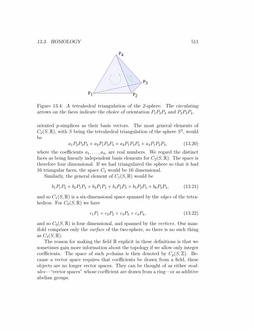
13.3. HOMOLOGY 511
1 2
3
4
P
P
P
P
Figure 13.4: A tetrahedral triangulation of the 2-sphere. The circulatingarrows on the faces indicate the choice of orientation P1P2P4 and P2P3P4.
oriented p-simplices as their basis vectors. The most general elements ofC2(S,R), with S being the tetrahedral triangulation of the sphere S2, wouldbe
a1P2P3P4 + a2P1P3P4 + a3P1P2P4 + a4P1P2P3, (13.20)
where the coefficients a1, . . . , a4, are real numbers. We regard the distinctfaces as being linearly independent basis elements for C2(S,R). The space istherefore four dimensional. If we had triangulated the sphere so that it had16 triangular faces, the space C2 would be 16 dimensional.
Similarly, the general element of C1(S,R) would be
b1P1P2 + b2P1P3 + b3P1P4 + b4P2P3 + b5P2P4 + b6P3P4, (13.21)
and so C1(S,R) is a six-dimensional space spanned by the edges of the tetra-hedron. For C0(S,R) we have
c1P1 + c2P2 + c3P3 + c4P4, (13.22)
and so C0(S,R) is four dimensional, and spanned by the vertices . Our man-ifold comprises only the surface of the two-sphere, so there is no such thingas C3(S,R).
The reason for making the field R explicit in these definitions is that wesometimes gain more information about the topology if we allow only integercoefficients. The space of such p-chains is then denoted by Cp(S,Z). Be-cause a vector space requires that coefficients be drawn from a field, theseobjects are no longer vector spaces. They can be thought of as either mod-ules—“vector spaces” whose coefficient are drawn from a ring—or as additiveabelian groups.

512CHAPTER 13. AN INTRODUCTION TO DIFFERENTIAL TOPOLOGY
P2 P3
P4
Figure 13.5: The oriented triangle P2P3P4 has boundary P3P4+P4P2+P2P3.
The boundary operator
We now introduce a linear map ∂p : Cp → Cp−1, called the boundary operator.Its action on a p-simplex is
∂pPi1Pi2 · · ·Pip+1=
p+1∑
j=1
(−1)j−1Pi1 . . . Pij . . . Pip+1, (13.23)
where the “hat” indicates that Pij is to be omitted. The resulting (p − 1)-chain is called the boundary of the simplex. For example
∂2(P2P3P4) = P3P4 − P2P4 + P2P3,
= P3P4 + P4P2 + P2P3. (13.24)
The boundary of a line segment is the difference of its endpoints
∂1(P1P2) = P2 − P1. (13.25)
Finally, for any point,∂0Pi = 0. (13.26)
Because ∂p is defined to be a linear map, when it is applied to a p-chainc = a1s1 + a2s2 + · · · + ansn, where the si are p-simplices, we have ∂pc =a1∂ps1 + a2∂ps2 + · · ·+ an∂psn.
When we take the “∂” of a chain of compatibly oriented simplices thattogether make up some region, the internal boundaries cancel in pairs, andthe “boundary” of the chain really is the oriented geometric boundary of theregion. For example, in figure 13.6 we find that
∂(P1P5P2+P2P5P4+P3P4P5+P1P3P5) = P1P3+P3P4+P4P2+P2P1, (13.27)

13.3. HOMOLOGY 513
P4
2PP1
P3
P5
Figure 13.6: Compatibly oriented simplices.
which is the anti-clockwise directed boundary of the square.For each of the examples above, we find that ∂p−1∂p s = 0. From the
definition (13.23) we can easily establish that this identity holds for any p-simplex s. As chains are sums of simplices and ∂p is linear, it remains truefor any c ∈ Cp. Thus ∂p−1∂p = 0. We will usually abbreviate this statementas ∂2 = 0.
Cycles, boundaries and homology
A chain complex is a doubly-infinite sequence of spaces (these can be vectorspaces, modules, abelian groups, or many other mathematical objects) suchas . . . , C−2, C−1, C0, C1, C2 . . ., together with structure-preserving maps
. . .∂p+1→ Cp
∂p→ Cp−1∂p−1→ Cp−2
∂p−1→ . . . , (13.28)
possessing the property that ∂p−1∂p = 0. The finite sequence of Cp’s that weconstructed from our simplicial complex is an example of a chain complexwhere Cp is zero-dimensional for p < 0 or p > d. Chain complexes are auseful tool in mathematics, and the ideas that we explain in this sectionhave many applications.
Given any chain complex we can define two important linear subspacesof each of the Cp’s. The first is the space Zp of p-cycles . This consists ofthose z ∈ Cp such that ∂pz = 0. The second is the space Bp of p-boundaries ,and consists of those b ∈ Cp such that b = ∂p+1c for some c ∈ Cp+1. Because∂2 = 0, the boundaries Bp constitute a subspace of Zp. From these spaceswe form the quotient space Hp = Zp/Bp, consisting of equivalence classes ofp-cycles, where we deem z1 and z2 to be equivalent, or homologous , if theydiffer by a boundary: z2 = z1 + ∂c. We write the equivalence class of cycles
514CHAPTER 13. AN INTRODUCTION TO DIFFERENTIAL TOPOLOGY
homologous zi to as [zi]. The space Hp, or more accurately, Hp(R), is calledthe p-th (simplicial) homology space of the chain complex. It becomes thep-th homology group if R is replaced by the integers.
We can construct these homology spaces for any chain complex. Whenthe chain complex is derived from a simplicial complex decomposition of amanifold M a remarkable thing happens. The spaces Cp, Zp, and Bp, alldepend on the details of how the manifold M has been dissected to formthe simplicial complex S. The homology space Hp, however, is independentof the dissection. This is neither obvious nor easy to prove. We will relyon examples to make it plausible. Granted this independence, we will writeHp(M), or Hp(M,R), so as to make it clear that Hp is a property of M . Thedimension bp of Hp(M) is called the p-th Betti number of the manifold:
bpdef= dimHp(M). (13.29)
Example: The Two-Sphere. For the tetrahedral dissection of the two-sphere,any vertex is Pi homologous to any other, as Pi − Pj = ∂(PjPi) and allPjPi belong to C2. Furthermore, ∂Pi = 0, so H0(S
2) is one dimensional.In general, the dimension of H0(M) is the number of disconnected piecesmaking up M . We will write H0(S
2) = R, regarding R as the archetype of aone-dimensional vector space.
Now let us consider H1(S2). We first find the space of 1-cycles Z1. An
element of C1 will be in Z1 only if each vertex that is the begining of an edgeis also the end of an edge, and that these edges have the same coefficient.Thus,
z1 = P2P3 + P3P4 + P4P2
is a cycle, as isz2 = P1P4 + P4P2 + P2P1.
These are both boundaries of faces of the tetrahedron. It should be fairlyeasy to convince yourself that Z1 is the space of linear combinations of thesetogether with boundaries of the other faces
z3 = P1P4 + P4P3 + P3P1,
z4 = P1P3 + P3P2 + P2P1.
Any three of these are linearly independent, and so Z1 is three dimensional.Because all of the cycles are boundaries, every element of Z1 is homologousto 0, and so H1(S
2) = 0.
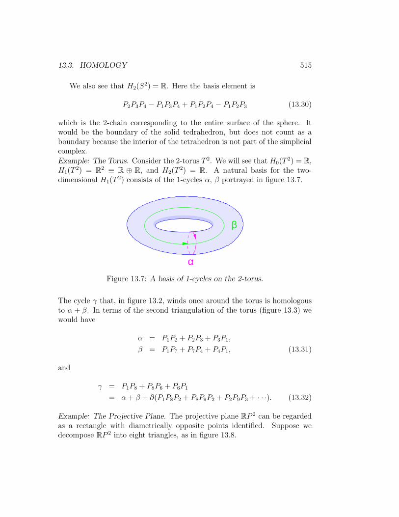
13.3. HOMOLOGY 515
We also see that H2(S2) = R. Here the basis element is
P2P3P4 − P1P3P4 + P1P2P4 − P1P2P3 (13.30)
which is the 2-chain corresponding to the entire surface of the sphere. Itwould be the boundary of the solid tedrahedron, but does not count as aboundary because the interior of the tetrahedron is not part of the simplicialcomplex.
Example: The Torus. Consider the 2-torus T 2. We will see that H0(T2) = R,
H1(T2) = R2 ≡ R ⊕ R, and H2(T
2) = R. A natural basis for the two-dimensional H1(T
2) consists of the 1-cycles α, β portrayed in figure 13.7.
α
β
Figure 13.7: A basis of 1-cycles on the 2-torus.
The cycle γ that, in figure 13.2, winds once around the torus is homologousto α + β. In terms of the second triangulation of the torus (figure 13.3) wewould have
α = P1P2 + P2P3 + P3P1,
β = P1P7 + P7P4 + P4P1, (13.31)
and
γ = P1P8 + P8P6 + P6P1
= α+ β + ∂(P1P8P2 + P8P9P2 + P2P9P3 + · · ·). (13.32)
Example: The Projective Plane. The projective plane RP 2 can be regardedas a rectangle with diametrically opposite points identified. Suppose wedecompose RP 2 into eight triangles, as in figure 13.8.

516CHAPTER 13. AN INTRODUCTION TO DIFFERENTIAL TOPOLOGY
P1
P1
P
P
P2
P2
3
P4P4
3
P5
Figure 13.8: A triangulation of the projective plane.
Consider the “entire surface”
σ = P1P2P5 + P1P5P4 + · · · ∈ C2(RP2), (13.33)
consisting of the sum of all eight 2-simplices with the orientation indicatedin the figure. Let α = P1P2 + P2P3 and β = P1P4 + P4P3 be the sides of therectangle running along the bottom horizontal and left vertical sides of thefigure, respectively. In each case they run from P1 to P3. Then
∂(σ) = P1P2 + P2P3 + P3P4 + P4P1 + P1P2 + P2P3 + P3P4 + P4P1
= 2(α− β) 6= 0. (13.34)
Although RP 2 has no actual edge that we can fall off, from the homologicalviewpoint it does have a boundary! This represents the conflict between localorientation of each of the 2-simplices and the global non-orientability of RP 2.The surface σ of RP 2 is not a two-cycle, therefore. Indeed Z2(RP 2), and afortiori H2(RP 2), contain only the zero vector. The only one-cycle is α− βwhich runs from P1 to P1 via P2, P3 and P4, but (13.34) shows that this isthe boundary of 1
2σ. Thus H2(RP 2,R) = 0 and H1(RP 2,R) = 0, while
H0(RP 2,R) = R.We can now see the advantage of restricting ourselves to integer coeffi-
cients. When we are not allowed fractions, the cycle γ = (α−β) is no longera boundary, although 2(α−β) is the boundary of σ. Thus, using the symbolZ2 to denote the additive group of the integers modulo two, we can writeH1(RP 2,Z) = Z2. This homology space is a set with only two members0γ, 1γ. The finite group H1(RP 2,Z) = Z2 is said to be the torsion partof the homology — a confusing terminology because this torsion has nothingto do with the torsion tensor of Riemannian geometry.

13.3. HOMOLOGY 517
We introduced real-number homology first, because the theory of vectorspaces is simpler than that of modules, and more familiar to physicists. Thetorsion is, however, invisible to the real-number homology. We were thereforebuying a simplification at the expense of throwing away information.
The Euler Character
The sum
χ(M)def=
d∑
p=0
(−1)p dimHp(M,R) (13.35)
is called the Euler character of the manifold M . For example, the 2-spherehas χ(S2) = 2, the projective plane has χ(RP 2) = 1, and the n-torus hasχ(T n) = 0. This number is manifestly a topological invariant because theindividual dimHp(M,R) are. We will show that that the Euler character isalso equal to V − E + F − · · · where V is the number of vertices, E is thenumber of edges and F is the number of faces in the simplicial dissection. Thedots are for higher dimensional spaces, where the alternating sum continueswith (−1)p times the number of p-simplices. In other words, we are claimingthat
χ(M) =d∑
p=0
(−1)p dimCp(M). (13.36)
It is not so obvious that this new sum is a topological invariant. The indi-vidual dimensions of the spaces of p-chains depend on the details of how wedissect M into simplices. If our claim is to be correct, the dependence mustsomehow drop out when we take the alternating sum.
A useful tool for working with alternating sums of vector-space dimensionsis provided by the notion of an exact sequence. We say that a set of vectorspaces Vp with maps fp : Vp → Vp+1 is an exact sequence if Ker (fp) =Im (fp−1). For example, if all cycles were boundaries then the set of spaces Cpwith the maps ∂p taking us from Cp to Cp−1 would consitute an exact sequence— albeit with p decreasing rather than increasing, but this is irrelevent.When the homology is non-zero, however, we only have Im (fp−1) ⊂ Ker (fp),and the number dimHp = dim (Ker fp) − dim (Im fp−1) provides a measureof how far this set inclusion falls short of being an equality.
Suppose that
0 f0−→ V1f1−→ V2
f2−→ . . .fn−1−→ Vn
fn−→ 0 (13.37)

518CHAPTER 13. AN INTRODUCTION TO DIFFERENTIAL TOPOLOGY
is a finite-length exact sequence. Here, 0 is the vector space containingonly the zero vector. Being linear, f0 maps 0 to 0. Also fn maps everythingin Vn to 0. Since this last map takes everything to zero, and what is mappedto zero is the image of the penultimate map, we have Vn = Im fn−1. Similarly,the fact that Ker f1 = Im f0 = 0 shows that Im f1 ⊆ V2 is an isomorphicimage of V1. This situation is represented pictorially in figure 13.9.
V1 V2 V3 V4 V5
fIm Im f Imf Imf
f0 f f f f4 f5
0
0 0 0
21 3 4
01 2 3
0 0 0 0
Figure 13.9: A schematic representation of an exact sequence.
Now the range-nullspace theorem tells us that
dimVp = dim (Im fp) + dim (Ker fp)
= dim (Im fp) + dim (Im fp−1). (13.38)
When we take the alternating sum of the dimensions, and use dim (Im f0) = 0and dim (Im fn) = 0, we find that the sum telescopes to give
n∑
p=0
(−1)p dim Vp = 0. (13.39)
The vanishing of this alternating sum is one of the principal properties of anexact sequence.
Now, for our sequence of spaces Cp with the maps ∂p : Cp → Cp−1, we havedim (Ker ∂p) = dim (Im ∂p+1) + dimHp. Using this and the range-nullspacetheorem in the same manner as above, shows that
d∑
p=0
(−1)pdimCp(M) =d∑
p=0
(−1)pdimHp(M). (13.40)
This confirms our claim.

13.3. HOMOLOGY 519
Exercise 13.1: Count the number of vertices, edges and faces in the triangu-lation we used to compute the homology groups of the real projective planeRP 2. Verify that V − E + F = 1, and that this is the same number that weget by evaluating
χ(RP 2) = dimH0(RP2,R)− dimH1(RP
2,R) + dimH2(RP2,R).
Exercise 13.2: Show that the sequence
0 → Vφ→W → 0
of vector spaces being exact means that the map φ : V → W is one-to-oneand onto, and hence an isomorphism V ∼=W .
Exercise 13.3: Show that a short exact sequence
0 → Ai→ B
π→ C → 0
of vector spaces is just a sophisticated way of asserting that C ∼= B/A. Moreprecisely, show that the map i is injective (one-to-one), so A can be consideredto be a subspace of B. Then show that the map π is surjective (onto), andcan be regarded as projecting B onto the equivalence classes B/A.
Exercise 13.4: Let α : A→ B be a linear map. Show that
0→Kerαi→ A
α→ Bπ→ Cokerα→ 0
is an exact sequence. (Recall that Cokerα ≡ B/Imα.)
13.3.2 Relative Homology
Mathematicians have invented powerful tools for computing homology. Inthis section we introduce one of them: the exact sequence of a pair . Wedescribe this tool in detail because a homotopy analogue of this exact se-quence is used in physics to classify defects such as dislocations, vortices andmonopoles. Homotopy theory is however harder and requires more technicalapparatus than homology, so the ideas are easier to explain here.
We have seen that it is useful to think of complicated manifolds as beingassembled out of simpler ones. We constructed the torus, for example, bygluing together edges of a rectangle. Another construction technique involves

520CHAPTER 13. AN INTRODUCTION TO DIFFERENTIAL TOPOLOGY
shrinking parts of a manifold to a point. Think, for example, of the unit 2-disc as a being circle of cloth with a drawstring sewn into its boundary. Nowpull the string tight to form a spherical bag. The continuous functions onthe resulting 2-sphere are those continuous functions on the disc that tookthe same value at all points on its boundary. Recall that we used this idea insection 12.4.2, where we claimed that those spin textures in R2 that point ina fixed direction at infinity can be thought of as spin textures on the 2-sphere.We now extend this shrinking trick to homology.
Suppose that we have a chain complex consisting of spaces Cp and bound-ary operations ∂p. We denote this chain complex by (C, ∂). Another set ofof spaces and boundary operations (C ′, ∂′) is a subcomplex of (C, ∂) if eachC ′p ⊆ Cp and ∂
′p(c) = ∂p(c) for each c ∈ C ′
p. This situation arises if we have asimplical complex S and a some subset S ′ that is itself a simplicial complex,and take C ′
p = Cp(S′)
Since each C ′p is subspace of Cp we can form the quotient spaces Cp/C
′p
and make them into a chain complex by defining, for c+ C ′p ∈ Cp/C ′
p,
∂p(c+ C ′p) = ∂pc + C ′
p−1. (13.41)
It easy to see that this operation is well defined (i.e. it gives the same outputindependent of the choice of representative in the equivalence class c + C ′
p),
that ∂p : Cp → Cp−1 is a linear map, and that ∂p−1∂p = 0. We haveconstructed a new chain complex (C/C ′, ∂). We can therefore form its ho-mology spaces in the usual way. The resulting vector space, or abelian group,Hp(C/C
′) is the p-th relative homology group of C modulo C ′. When C ′ andC arise from simplicial complexes S ′ ⊆ S, these spaces are what remains ofthe homology of S after every chain in S ′ has been shrunk to a point. Inthis case, it is customary to write Hp(S, S
′) instead of Hp(C/C′), and simi-
larly write the chain, cycle and boundary spaces as Cp(S, S′), Zp(S, S
′) andBp(S, S
′) respectively.Example: Constructing the two-sphere S2 from the two-ball (or disc) B2.We regard B2 to be the triangular simplex P1P2P3, and its boundary, theone-sphere or circle S1, to be the simplicial complex containing the points P1,P2, P3 and the sides P1P2, P2P3, P3P1, but not the interior of the triangle.We wish to contract this boundary complex to a point, and form the relativechain complexes and their homology spaces. Of the spaces we quotient by,C0(S
1) is spanned by the points P1, P2, P3, the 1-chain space C1(S1) is
spanned by the sides P1P2, P2P3, P3P1, while C2(S1) = 0. The space of

13.3. HOMOLOGY 521
relative chains C2(B1, S1) consists of multiples of P1P2P3 + C2(S
1), and theboundary
∂2
(P1P2P3 + C2(S
1))= (P2P3 + P3P1 + P1P2) + C1(S
1) (13.42)
is equivalent to zero because P2P3 + P3P1 + P1P2 ∈ C1(S1). Thus P1P2P3 +
C2(S1) is a non-bounding cycle and spans H2(B
2, S1), which is thereforeone dimensional. This space is isomorphic to the one-dimensional H2(S
2).Similarly H1(B
2, S1) is zero dimensional, and so isomorphic to H1(S2). This
is because all chains in C1(B2, S1) are in C1(S
1) and therefore equivalent tozero.
A peculiarity, however, is that H0(B2, S1) is not isomorphic to H0(S
2) =R. Instead, we find that H0(B
2, S1) = 0 because all the points are equiva-lent to zero. This vanishing is characteristic of the zeroth relative homologyspace H0(S, S
′) for the simplicial triangulation of any connected manifold.It occurs because S being connected means that any point P in S can bereached by walking along edges from any other point, in particular from apoint P ′ in S ′. This makes P homologous to P ′, and so equivalent to to zeroin H0(S, S
′).
Exact homology sequence of a pair
Homological algebra is full of miracles. Here we describe one of them. Fromthe ingredients we have at hand, we can construct a semi-infinite sequenceof spaces and linear maps between them
· · · ∂∗p+1−→ Hp(S′)
i∗p−→ Hp(S)π∗p−→ Hp(S, S
′)∂∗p−→
Hp−1(S′)i∗p−1−→ Hp−1(S)
π∗p−1−→ Hp−1(S, S′)∂∗p−1−→
...∂∗1−→ H0(S
′)i∗0−→ H0(S)
π∗0−→ H0(S, S′)
∂∗0−→ 0. (13.43)
The maps i∗p and π∗p are induced by the natural injection ip : Cp(S′)→ Cp(S)
and projection πp : Cp(S)→ Cp(S)/Cp(S′). It is only necessary to check that
πp−1∂p = ∂pπp,
ip−1∂p = ∂pip, (13.44)

522CHAPTER 13. AN INTRODUCTION TO DIFFERENTIAL TOPOLOGY
to see that they are compatible with the passage from the chain spaces tothe homology spaces. More discussion is required of the connection map ∂∗pthat takes us from one row to the next in the displayed form of (13.43).
The connection map is constructed as follows: Let h ∈ Hp(S, S′). Then
h = z + Bp(S, S′) for some cycle z ∈ Z(S, S ′), and in turn z = c + Cp(S
′)for some c ∈ Cp(S). (So two choices of representative of equivalence classare being made here.) Now ∂pz = 0 which means that ∂pc ∈ Cp−1(S
′). Thisfact, when combined with ∂p−1∂p = 0, tells us that ∂pc ∈ Zp−1(S
′). We nowdefine the ∂∗p image of h to be
∂∗p(h) = ∂pc+Bp−1(S′). (13.45)
This sounds rather involved, but let’s say it again in words: an element ofHp(S, S
′) is a relative p-cycle modulo S ′. This means that its boundary isnot necessarily zero, but may be a non-zero element of Cp−1(S
′). Since thiselement is the boundary of something its own boundary vanishes, so it is(p − 1)-cycle in Cp−1(S
′) and hence a representative of a homology class inHp−1(S
′). This homology class is the output of the ∂∗p map.The miracle is that the sequence of maps (13.43) is exact . It is an example
of a standard homological algebra construction of a long exact sequence outof a family of short exact sequences, in this case out the sequences
0 → Cp(S′)→ Cp(S)→ Cp(S, S
′)→ 0. (13.46)
Proving that the long sequence is exact is straightforward. All one must dois check each map to see that it has the properties required. This exercise inwhat is called diagram chasing is left to the reader.
The long exact sequence that we have constructed is called the exacthomology sequence of a pair . If we know that certain homology spaces arezero dimensional, it provides a powerful tool for computing other spaces inthe sequence. As an illustration, consider the sequence of the pair Bn+1 andSn for n > 0:
· · · i∗p−→ Hp(Bn+1)︸ ︷︷ ︸
= 0
π∗p−→ Hp(Bn+1, Sn)
∂∗p−→ Hp−1(Sn)
i∗p−1−→ Hp−1(Bn+1)︸ ︷︷ ︸
= 0
π∗p−1−→ Hp−1(Bn+1, Sn)
∂∗p−1−→ Hp−2(Sn)

13.3. HOMOLOGY 523
...i∗1−→ H1(B
n+1)︸ ︷︷ ︸= 0
π∗1−→ H1(Bn+1, Sn)
∂∗1−→ H0(Sn)︸ ︷︷ ︸
= Ri∗0−→ H0(B
n+1)︸ ︷︷ ︸= R
π∗0−→ H0(Bn+1, Sn)
∂∗0−→ 0. (13.47)
We have inserted here the easily-established data that Hp(Bn+1) = 0 for
p > 0 (which is a consequence of the (n+1)-ball being a contractible space),and that H0(B
n+1) and H0(Sn) are one dimensional because they consist of
a single connected component. We read off, from the 0 → A→ B → 0exact subsequences, the isomorphisms
Hp(Bn+1, Sn) ∼= Hp−1(S
n), p > 1, (13.48)
and from the exact sequence
0 → H1(Bn+1, S1)→ R→ R→ H0(B
n+1, Sn)→ 0 (13.49)
that H1(Bn+1, Sn) = 0 = H0(B
n+1, Sn). The first of these equalities holdsbecause H1(B
n+1, Sn) is the kernel of the isomorphism R → R, and thesecond because H0(B
n+1, Sn) is the range of a surjective null map.In the case n = 0, we have to modify our last conclusion becauseH0(S
0) =R ⊕ R is two dimensional. (Remember that H0(M) counts the number ofdisconnected components of M , and the zero-sphere S0 consists of the twodisconnected points P1, P2 lying in the boundary of the interval B1 = P1P2.)As a consequence, the last five maps in (13.47) become
0 → H1(B1, S0)→ R⊕ R→ R→ H0(B
1, S0)→ 0. (13.50)
This tells us that H1(B1, S0) = R and H0(B
1, S0) = 0.
Exact homotopy sequence of a pair
The construction of a long exact sequence from a short exact sequence isa very powerful technique. It has become almost ubiquitous in advancedmathematics. Here we briefly describe an application to homotopy theory.
We have met the homotopy groups πn(M) in section 12.4.4. As we sawthere, homotopy groups can be used to classify defects or textures in physical
524CHAPTER 13. AN INTRODUCTION TO DIFFERENTIAL TOPOLOGY
systems in which some field takes values in a manifold M . Suppose that thelocal physical properties of a system are invariant under the action of a Liegroup G — for example the high temperature phase of ferromagnet may beinvariant under rotation group SO(3)). Now suppose that system undergoesspontaneous symmetry breaking is becomes invariant only under a subgroupH . Then manifold manifold of inequivalent states is the coset G/H . Fora ferromagnet the symmetry breaking will from G = SO(3) to H = SO(2)where SO(2) is the group of rotations about the axis of magnetization. G/His then the 2-sphere of direction in which the magnetization can point.
The group πn(G) can be taken to be the set of continuous maps of ann-dimensional cube into the group G, with the surface of the cube mappingto the identity element e ∈ G. We similarly define the relative homotopygroup πn(G,H) of G modulo H to be the set of continuous maps of thecube into G, with all-but-one face of the cube mapping to e, but with theremaining face mapping to the subgroup H . It can then be shown thatπn(G/H) ∼= πn(G,H) (the hard part is to show that any continuous mapinto G/H can be represented as the projection of some continuous map intoG).
The short exact sequence
e → Hi→ G
π→ G/H → e (13.51)
of group homomorphisms (where e is the group consisting only of theidentity element) then gives rise to the long exact sequence
· · · → πn(H)→ πn(G)→ πn(G,H)→ πn−1(H)→ · · · . (13.52)
The derivation and utility of this exact sequence is very well described inthe review article by Mermin cited in section 12.4.4. We have thereforecontented ourselves with simply displaying the result so that the reader cansee the similarity between the homology theorem and its homotopy-theoryanalogue.
13.4 De Rham’s Theorem
We still have not related homology to cohomology. The link is provided byintegration.

13.4. DE RHAM’S THEOREM 525
The integral provides a natural pairing of a p-chain c and a p-form ω: ifc = a1s1 + a2s2 + · · ·+ ansn, where the si are simplices, we set
(c, ω) =∑
i
ai
∫
si
ω. (13.53)
The perhaps mysterious notion of “adding” geometric simplices is thus givena concrete interpretation in terms of adding real numbers.
Stokes’ theorem now reads
(∂c, ω) = (c, dω), (13.54)
suggesting that d and ∂ should be regarded as adjoints of each other. Fromthis observation follows the key fact that the pairing between chains andforms descends to a pairing between homology classes and cohomology classes.In other words,
(z + ∂c, ω + dχ) = (z, ω), (13.55)
so it does not matter which representatives of the two equivalence classes wetake when we compute the integral. Let us see why this is so.
Suppose z ∈ Zp and ω2 = ω1 + dη. Then
(z, ω2) =
∫
z
ω2 =
∫
z
ω1 +
∫
z
dη
=
∫
z
ω1 +
∫
∂z
η
=
∫
z
ω1
= (z, ω1) (13.56)
because ∂z = 0. Thus, all elements of the cohomology class of ω return thesame answer when integrated over a cycle.
Similarly, if ω ∈ Zp and c2 = c1 + ∂a then
(c2, ω) =
∫
c1
ω +
∫
∂a
ω
=
∫
c1
ω +
∫
a
dω
=
∫
c1
ω
= (c1, ω),

526CHAPTER 13. AN INTRODUCTION TO DIFFERENTIAL TOPOLOGY
since dω = 0.All this means that we can consider the equivalence classes of closed forms
composing HpdR(M) to be elements of (Hp(M))∗, the dual space of Hp(M)
— hence the “co” in cohomology. The existence of the pairing does notautomatically mean that Hp
dR is the dual space to Hp(M), however, becausethere might be elements of the dual space that are not in Hp
dR, and theremight be distinct elements ofHp
dR that give identical answers when integratedover any cycle, and so correspond to the same element in (Hp(M))∗. Thisdoes not happen, however, when the manifold is compact : De Rham showedthat, for compact manifolds, (Hp(M,R))∗ = Hp
dR(M,R). We will not try toprove this, but be satisfied with some examples.
The statement (Hp(M))∗ = HpdR(M) neatly summarizes de Rham’s re-
sults, but, in practice, the more explicit statements given below are moreuseful.
Theorem: (de Rham) Suppose that M is a compact manifold.1) A closed p-form ω is exact if and only if
∫
zi
ω = 0 (13.57)
for all cycles zi ∈ Zp. It suffices to check this for one representative ofeach homology class.
2) If zi ∈ Zp, i = 1, . . . , dimHp, is a basis for the p-th homology space,and αi a set of numbers, one for each zi, then there exists a closedp-form ω such that ∫
zi
ω = αi. (13.58)
If ωi constitute a basis of the vector space Hp(M) then the matrix of numbers
Ωij = (zi, ω
j) =
∫
zi
ωj (13.59)
is called the period matrix , and the Ωij themselves are the periods .
Example: H1(T2) = R ⊕ R is two dimensional. Since a finite-dimensional
vector space and its dual have the same dimension, de Rham tells us thatH1
dR(T2) is also two-dimensional. If we take as coordinates on T 2 the angles
θ and φ, then the basis elements, or generators , of the cohomology spaces arethe forms “dθ” and “dφ”. We have inserted the quotes to stress that these

13.4. DE RHAM’S THEOREM 527
expressions are not the d of a function. The angles θ and φ are not functionson the torus, since they are not single-valued. The homology basis 1-cyclescan be taken as zθ running from θ = 0 to θ = 2π along φ = π, and zφ runningfrom φ = 0 to φ = 2π along θ = π. Clearly, ω = αθdθ/2π+αφdφ/2π returns∫zθω = αθ and
∫zφω = αφ for any αθ, απ, so dθ/2π, dφ/2π and zθ, zφ are
dual bases.Example: We have earlier computed the homology groups H2(RP 2,R) = 0and H1(RP 2,R) = 0. De Rham therefore tells us that H2(RP 2,R) = 0and H1(RP 2,R) = 0. From this we deduce that all closed one- and two-forms on the projective plane RP 2 are exact.Example: As an illustration of de Rham part 1), observe that it is easy toshow that a closed one-form φ can be written as df , provided that
∫ziφ = 0
for all cycles. We simply define f =∫ xx0φ, and observe that the proviso
ensures that f is not multivalued.Example: A more subtle problem is to show that, given a two-form ω on S2,with
∫S2 ω = 0 there is a globally-defined χ such that ω = dχ. We begin
by covering S2 by two open sets D+ and D− which have the form of capssuch that D+ includes all of S2 except for a neighbourhood of the southpole, while D− includes all of S2 except a neighbourhood of the north pole,and the intersection, D+ ∩D−, has the topology of an annulus, or cingulum,encircling the equator.
D
D
+
_
Γ
Figure 13.10: A covering the 2-sphere by a pair of contractable caps.
Since both D+ and D− are contractable, there are one-forms χ+ and χ− suchthat ω = dχ+ in D+ and ω = dχ− in D−. Thus,
d(χ+ − χ−) = 0, in D+ ∩D−. (13.60)

528CHAPTER 13. AN INTRODUCTION TO DIFFERENTIAL TOPOLOGY
Dividing the sphere into two disjoint sets with a common (but opposinglyoriented) boundary Γ ∈ D+ ∩D−, we have
0 =
∫
S2
ω =
∮
Γ
(χ+ − χ−), (13.61)
and this is true for any such curve Γ. Thus, by the previous example,
φ ≡ (χ+ − χ−) = df (13.62)
for some smooth function f defined inD+∩D−. We now introduce a partitionof unity subordinate to the cover of S2 by D+ and D−. This partition is apair of non-negative smooth functions, ρ±, such that ρ+ is non-zero only inD+, ρ− is non-zero only in D−, and ρ+ + ρ− = 1. Now
f = ρ+f − (−ρ−)f, (13.63)
and f− = ρ+f is a function defined everywhere on D−. Similarly f+ =(−ρ−)f is a function on D+. Notice the interchange of ± labels! This is nota mistake. The function f is not defined outside D+∩D−, but we can defineρ−f everywhere on D+ because f gets multiplied by zero wherever we haveno specific value to assign to it. We now observe that
χ+ + df+ = χ− + df−, in D+ ∩D−. (13.64)
Thus ω = dχ, where χ is defined everywhere by the rule
χ =
χ+ + df+, in D+,χ− + df−, in D−.
(13.65)
It does not matter which definition we take in the cingular region D+ ∩D−,because the two definitions coincide there.
The methods of this example can be extended to give a proof of de Rham’sclaims.
13.5 Poincare Duality
De Rham’s theorem does not require that our manifoldM be orientable. Ournext results do, however, require orientablity. We therefore assume through-out this section that M is a compact, orientable, D-dimensional manifold.

13.5. POINCARE DUALITY 529
We will also require that M is a closed manifold —- meaning that it has noboundary.
We begin with the observation that if the forms ω1 and ω2 are closed thenso is ω1∧ω2. Furthermore, if one or both of ω1, ω2 is exact then the productω1∧ω2 is also exact. It follows that the cohomology class [ω1∧ω2] of ω1∧ω2
depends only on the cohomology classes [ω1] and [ω2]. The wedge productthus induces a map
Hp(M,R)×Hq(M,R)∧→ Hp+q(M,R), (13.66)
which is called the “cup product” of the cohomology classes. It is writtenas
[ω1 ∧ ω2] = [ω1] ∪ [ω2], (13.67)
and gives the cohomology the structure of a graded-commutative ring, de-noted by H•(M,R)
More significant for us than the ring structure is that, given ω ∈ HD(M,R),we can obtain a real number by forming
∫Mω (This is the point at which
we need orientability. We only know how to integrate over orientable chains,and so cannot even define
∫Mω when M is not orientable) and can com-
bine this integral with the cup product to make any cohomology class [f ] ∈HD−p(M,R) into an element F of (Hp(M,R))∗. We do this by setting
F ([g]) =
∫
M
f ∧ g (13.68)
for each [g] ∈ Hp(M,R). Furthermore, it is possible to show that we canget any element F of (Hp(M,R))∗ in this way, and the corresponding [f ] isunique. But de Rham has already given us a way of identifying the elementsof (Hp(M,R))∗ with the cycles in Hp(M,R)! There is, therefore, a 1-1 ontomap
Hp(M,R)↔ HD−p(M,R). (13.69)
In particular the dimensions of these two spaces must coincide:
bp(M) = bD−p(M). (13.70)
This equality of Betti numbers is called Poincare duality . Poincare originallyconceived of it geometrically. His idea was to construct from each simplicialtriangulation S ofM a new “dual” triangulation S ′, where, in two dimensions

530CHAPTER 13. AN INTRODUCTION TO DIFFERENTIAL TOPOLOGY
for example, we place a new vertex at the centre of each triangle, and join thevertices by lines through each side of the old triangles to make new cells —each new cell containing one of the old vertices. If we are lucky, this processwill have the effect of replacing each p-simplex by a (D− p)-simplex, and soset up a map between Cp(S) and CD−p(S
′) that turns the homolgy “upsidedown.” The new cells are not always simplices, however, and it is hard tomake this construction systematic. Poincare’s original recipe was flawed.
Our present approach to Poincare’s result is asserting that for each basisp-cycle class [zpi ] there is a unique (up to cohomology) (D − p)-form ωD−p
i
such that ∫
zpi
f =
∫
M
ωD−pi ∧ f. (13.71)
We can construct this ωD−pi “physically” by taking a representative cycle zpi
in the homology class [zpi ] and thinking of it as a surface with a conservedunit (d − p)-form current flowing in its vicinity. An example would be thetwo-form topological current running along the one-dimensional worldline ofa skyrmion. (See the discussion surrounding equation (12.64).) The ωD−p
i
form a basis for HD−p(M,R). We can therefore expand f ∼ f iωD−pi , and
similarly for the closed p-form g, to obtain
∫
M
g ∧ f = f igjI(i, j), (13.72)
where the matrix
I(i, j)def= I(zpi , z
D−pj ) =
∫
M
ωD−pi ∧ ωpj (13.73)
is called the intersection form. From its definition we see that I(i, j) satisfiesthe symmetry
I(i, j) = (−1)p(D−p)I(j, i). (13.74)
Less obvious is that I(i, j) is an integer that reports the number of times(counted with orientation) that the cycles zpi and zD−p
j intersect. This latterfact can be understood from our construction of the ωpi as unit currents lo-calized near the zD−p
i cycles. The integrand in (13.73) is non-zero only in theneighbourhood of the intersections of zpi with zD−p
j , and at each intersectionconstitutes a D-form that integrates up to give ±1.

13.5. POINCARE DUALITY 531
+1 +1−1+1 α α
β β
Figure 13.11: The intersection of two cycles: I(α, β) = 1 = 1− 1 + 1.
This claim is illustrated in the left-hand part of figure 13.11, which shows aregion surrounding the intersection of the α and β one-cycles on the 2-torus.The co-ordinate system has been chosen so that the α cycle runs along thex axis and the β cycle along then y axis. Each cycle is surrounded by thenarrow shaded regions −w < y < w and −w < x < w, respectively. Toconstruct suitable forms ωα and ωβ we select a smooth function f(x) thatvanishes for |x| ≥ w and such that
∫f dx = 1. In the local chart we can then
set
ωα = f(y) dy,
ωβ = −f(x) dx,
both these forms being closed. The intersection number is given by theintegral
I(α, β) =
∫ωα ∧ ωβ =
∫∫f(x)f(y) dxdy = 1. (13.75)
The right-hand part of figure 13.11 illustrates why this intersection numberdepends only on the homology classes of the two one-cycles, and not on theirparticular instantiation as curves.
We can more conveniently re-express (13.72) in terms of the periods ofthe forms
fidef=
∫
zpi
f = I(i, k)fk, gjdef=
∫
zD−pj
g = I(j, l)gl, (13.76)
as ∫
M
f ∧ g =∑
i,j
K(i, j)
∫
zpi
f
∫
zD−pj
g, (13.77)

532CHAPTER 13. AN INTRODUCTION TO DIFFERENTIAL TOPOLOGY
whereK(i, j) = I−1(i, k)I−1(j, l)I(k, l) = I−1(j, i) (13.78)
is the transpose of the inverse of the intersection-form matrix. The decom-position (13.77) of the integral of the product of a pair of closed forms intoa bilinear form in their periods is one of the two principal results of thissection, the other being (13.70).
In simple cases, we can obtain the decomposition (13.77) by more directmethods. Suppose, for example, that we label the cycles generating thehomology group H1(T
2) of the 2-torus as α and β, and that a and b areclosed (da = db = 0), but not necessarily exact, one-forms. We will showthat ∫
T 2
a ∧ b =∫
α
a
∫
β
b−∫
α
b
∫
β
a. (13.79)
To do this, we cut the torus along the cycles α and β and open it out intoa rectangle with sides of length Lx and Ly. The cycles α and β will formthe sides of the rectangle, and we will take them as lying parallel to the xand y axes, respectively. Functions on the torus now become functions onthe rectangle. Not all functions on the rectangle descend from functions onthe torus, however. Only those functions that satisfy the periodic bound-ary conditions f(0, y) = f(Lx, y) and f(x, 0) = f(x, Ly) can be considered(mathematicians would say “can be lifted”) to be functions on the torus.
2T
αα
α
β ββ
Figure 13.12: Cut-open torus
Since the rectangle (but not the torus) is retractable, we can write a = dfwhere f is a function on the rectangle — but not necessarily a function onthe torus, i.e. f will not, in general, be periodic. Since a∧ b = d(fb), we cannow use Stokes’ theorem to evaluate∫
T 2
a ∧ b =∫
T 2
d(fb) =
∫
∂T 2
fb. (13.80)
13.6. CHARACTERISTIC CLASSES 533
The two integrals on the two vertical sides of the rectangle can be combinedto a single integral over the points of the one-cycle β:
∫
vertical
fb =
∫
β
[f(Lx, y)− f(0, y)]b. (13.81)
We now observe that [f(Lx, y)− f(0, y)] is a constant, and so can be takenout of the integral. It is a constant because all paths from the point (0, y) to(Lx, y) are homologous to the one-cycle α, so the difference f(Lx, y)−f(0, y)is equal to
∫αa. Thus,
∫
β
[f(Lx, y)− f(0, y)]b =∫
α
a
∫
β
b. (13.82)
Similarly, the contributions of the two horizontal sides is∫
α
[f(x, 0)− f((x, Ly)]b = −∫
β
a
∫
α
b. (13.83)
On putting the contributions of both pairs of sides together, the claimedresult follows.
13.6 Characteristic Classes
A supply of elements ofH2m(M,R) andH2m(M,Z) is provided by the charac-teristic classes associated with connections on vector bundles over the man-ifold M .
Recall that connections appear in covariant derivatives
∇µdef= ∂µ + Aµ, (13.84)
and are to be thought of as matrix-valued one-forms A = Aµdxµ. In the
quantum mechanics of charged particles the covariant derivative that appearsin the Schrodinger equation is
∇µ =∂
∂xµ− ieAMaxwell
µ . (13.85)
Here, e is the charge of the particle on whose wavefunction the derivativeacts, and AMaxwell
µ is the usual electromagnetic vector potential. The matrix-valued connection one-form is therefore
A = −ieAMaxwellµ dxµ. (13.86)

534CHAPTER 13. AN INTRODUCTION TO DIFFERENTIAL TOPOLOGY
In this case the matrix is one-by-one.
In a non-abelian gauge theory with gauge groupG the connection becomes
A = iλaAaµdx
µ (13.87)
The λa are hermitian matrices that have commutation relations [λa, λb] =
if cabλc, where the f cab are the structure constants of the Lie algebra of the
group G. The λa therefore form a representation of the Lie algebra, andthis representation plays the role of the “charge” of the non-abelian gaugeparticle.
For covariant derivatives acting on a tangent vector field faea on a Rie-mann n-manifold, where the ea are an orthonormal vielbein frame, we have
A = ωabµdxµ, (13.88)
where, for each µ, the coefficients ωabµ = −ωbaµ can be thought of as theentries in a skew symmetric n-by-n matrix. These matrices are elements ofthe Lie algebra o(n) of the orthogonal group O(n).
In all these cases we define the curvature two-form to be F = dA + A2,where a combined matrix and wedge product is to be understood in A2. Inexercises 11.19 and 11.20 you used the Bianchi identity to show that thegauge-invariant 2n-forms tr (F n) were closed. The integrals of these formsover cycles provide numbers that are topological invariants of the bundle.For example, in four-dimensional QCD, the integral
c2 = −1
8π2
∫
Ω
tr (F 2) (13.89)
over a compactified four-dimensional manifold Ω is an integer that a mathe-matician would call the second Chern number of the non-abelian gauge bun-dle, and that a physicist would call the instanton number of the gauge fieldconfiguration. The closed forms themselves are called characteristic classes .
In the following section we will show that the integrals of characteristicclasses are indeed topological invariants. We also explain something of whatthese invariants are measuring, and illustrate why, when suitably normalized,they are integer-valued.

13.6. CHARACTERISTIC CLASSES 535
13.6.1 Topological invariance
Suppose that we have been given a connection A and slightly deform itA→ A + δA. Then F → F + δF where
δF = d(δA) + δAA+ AδA. (13.90)
Using the Bianchi identity dF = FA− AF , we find that
δ tr(F n) = n tr(δF F n−1)
= n tr(d(δA)F n−1) + n tr(δAAF n−1) + n tr(AδAF n−1)
= n tr(d(δA)F n−1) + n tr(δAAF n−1)− n tr(δAF n−1A)
= dn tr(δAF n−1)
. (13.91)
The last line of (13.91) is equal to the penultimate line because all but thefirst and last terms arising from the dF ’s in d tr(δAF n−1) cancel in pairs. Aglobally-defined change in A therefore changes tr(F n) by the d of something,and so does not change its cohomology class, or its integral over a cycle.
At first sight, this invariance under deformation suggests that all thetr(F n) are exact forms — they can apparently all be written as tr(F n) =dω2n−1(A) for some (2n− 1)-form ω2n−1(A). To find ω2n−1(A) all we have todo is deform the connection to zero by setting At = t A and
Ft = dAt + A2t = tdA+ t2A2. (13.92)
Then δAt = Aδt, and
d
dttr(F n
t ) = dn tr(AF n−1
t ). (13.93)
Integrating up from t = 0, we find
tr(F n) = d
n
∫ 1
0
tr(AF n−1t ) dt
. (13.94)
For example
tr(F 2) = d
2
∫ 1
0
tr(A(tdA+ t2A2) dt
= d
tr
(AdA +
2
3A3
). (13.95)

536CHAPTER 13. AN INTRODUCTION TO DIFFERENTIAL TOPOLOGY
You should recognize here the ω3(A) = tr(AdA + 23A3) Chern-Simons form
of exercise 11.19. The naıve conclusion — that all the tr(F n) are exact— is false, however. What the computation actually shows is that when∫tr(F n) 6= 0 we cannot find a globally defined one-form A representing the
connection or gauge field. With no global A, we cannot globally deform Ato zero.
Consider, for example, an Abelian U(1) gauge field on the two-sphere S2.When the first Chern-number
c1 =1
2πi
∫
S2
F (13.96)
is non-zero, there can be no globally-defined one-form A such that F =dA. Glance back, however, at figure 13.10 on page 527. There we see thatthe retractability of the spherical caps D± guarantees that there are one-forms A± defined on D± such that F = dA± in D±. In the cingular regionD+∩D− where they are both defined, A+ and A− will be related by a gaugetransformation. For a U(1) gauge field, the matrix g appearing in the generalgauge transformation rule
A→ Ag ≡ g−1Ag + g−1dg, (13.97)
of exercise 11.20 becomes the phase eiχ ∈ U(1). Consequently
A+ = A− + e−iχdeiχ = A− + idχ in D+ ∩D−. (13.98)
The U(1) group element eiχ is required to be single valued in D+ ∩D−, butthe angle χ may be multivalued. We now write c1 as the sum of integrals overthe north and south hemispheres of S2, and use Stokes theorem to reducethis sum to a single integral over the hemispheres’ common boundary, theequator Γ:
c1 =1
2πi
∫
north
F +1
2πi
∫
south
F
=1
2πi
∫
north
dA+ +1
2πi
∫
south
dA−
=1
2πi
∫
Γ
A+ −1
2πi
∫
Γ
A−
=1
2π
∫
Γ
dχ (13.99)

13.6. CHARACTERISTIC CLASSES 537
We see that c1 is an integer that counts the winding of χ as we circle Γ. Anon-zero integer cannot be continuously reduced to zero, and if we attemptto deform A→ tA→ 0, we will violate the required single-valuedness of theU(1) group element eiχ.
Although the Chern-Simons forms ω2n−1(A) cannot be defined globally,they are still very useful in physics. They occur as Wess-Zumino termsdescribing the low-energy properties of various quantum field theories, theprototype being the Skyrme-Witten model of Hadrons.3
13.6.2 Chern characters and Chern classes
Any gauge-invariant polynomial (with exterior multiplication of forms un-derstood) in F provides a closed, topologically invariant, differential form.Certain combinations, however, have additional desirable properties, and sohave been given names.
The form
chn(F ) = tr
1
n!
(i
2πF
)n(13.100)
is called the n-th Chern character . It is convenient to think of this 2n-formas being the n-th term in a generating-function expansion
ch(F )def= tr
exp
(i
2πF
)= ch0(F ) + ch1(F ) + ch2(F ) + · · · , (13.101)
where ch0(F )def= tr I is the dimension of the space on which the λa act. This
formal sum of forms of different degree is called the total Chern character .The n! normalization is chosen because it makes the Chern character behavenicely when we combine vector bundles — as we now do.
Given two vector bundles over the same manifold, having fibres Ux and Vxover the point x, we can make a new bundle with the direct sum Ux ⊕ Vx asfibre over x. This resulting bundle is called the Whitney sum of the bundles.Similarly we can make a tensor-product bundle whose fibre over x is Ux⊗Vx.
Let us use the notation ch(U) to represent the Chern character of thebundle with fibres Ux, and U ⊕V to denote the Whitney sum. Then we have
ch(U ⊕ V ) = ch(U) + ch(V ), (13.102)
3E. Witten, Nucl. Phys. B223 (1983) 422; ibid. B223 (1983) 433.

538CHAPTER 13. AN INTRODUCTION TO DIFFERENTIAL TOPOLOGY
andch(U ⊗ V ) = ch(U) ∧ ch(V ). (13.103)
The second of these formulæ comes about because if λ(1)a is a Lie algebra
element acting on V (1) and λ(2)a the corresponding element acting on V (2),
then they act on the tensor product V (1) ⊗ V (2) as
λ(1⊗2)a = λ(1)a ⊗ I + I ⊗ λ(2)a , (13.104)
where I is the identity operator on the appropriate space in the tensor prod-uct, and for matrices A and B we have
tr exp (A⊗ I + I ⊗B) = tr expA⊗ expB = tr expA tr expB .(13.105)
In terms of the individual chn(V ) equations (13.102) and (13.103) read
chn(U ⊕ V ) = chn(U) + chn(V ), (13.106)
and
chn(U ⊗ V ) =n∑
m=0
chn−m(U) ∧ chm(V ). (13.107)
Related to the Chern characters are the Chern classes . These are wedge-product polynomials in the Chern characters, and are defined, via the matrixexpansion
det (I + A) = 1 + trA+1
2
((trA)2 − trA2
)+ . . . , (13.108)
by the generating function for the total Chern class:
c(F ) = det
(I +
i
2πF
)= 1 + c1(F ) + c2(F ) + · · · . (13.109)
Thus
c1(F ) = ch1(F ), c2(F ) =1
2ch1(F ) ∧ ch1(F )− ch2(F ), (13.110)
and so on.For matrices A and B we have det(A ⊕ B) = det(A) det(B), and this
leads toc(U ⊕ V ) = c(U) ∧ c(V ). (13.111)

13.6. CHARACTERISTIC CLASSES 539
Although the Chern classes are more complicated in appearance than theChern characters, they are introduced because their integrals over cycles turnout to be integers , and this property remains true of integer-coefficient sumsof products of Chern-classes. The cohomology classes [cn(F )] are thereforeelements of the integer cohomology ring H•(M,Z). This property does nothold for the Chern characters, whose integrals over cycles can be fractions.The cohomology classes [chn(F )] are therefore only elements of H•(M,Q).
When we integrate products of Chern classes of total degree 2m overclosed 2m-dimensional orientable manifolds we get integer Chern numbers .These integers can be related to generalized winding numbers, and character-ize the extent to which the gauge transformations that relate the connectionfields in different patches serve to twist the vector bundle. Unfortunatelyit requires a considerable amount of combinatorial machinery (the Schubertcalculus of complex Grassmannians) to explain these integers.
Pontryagin and Euler classes
When the fibres of a vector bundle are vector spaces over R, the complexskew-hermitian matrices iλa are replaced by real skew symmetric matrices.The Lie algebra of the n-by-n matrices iλa was a subalgebra of u(n). The Liealgebra of the n-by-n real, skew symmetric, matrices is a subalgebra of o(n).Now, the trace of an odd power of any skew symmetric matrix is zero. As aconsequence, Chern characters and Chern classes containing an odd numberof F ’s all vanish. The remaining real 4n-forms are known as Pontryaginclasses . The precise definition is
pk(V )def= (−1)kc2k(V ). (13.112)
Pontryagin classes help to classify bundles whose gauge transformationsare elements of O(n). If we restrict ourselves to gauge transformations that liein SO(n), as we would when considering the tangent bundle of an orientableRiemann manifold, then we can make a gauge-invariant polynomial out ofthe skew-symmetric matrix-valued F by forming its Pfaffian.
Recall (or see exercise A.18) that the Pfaffian of a skew symmetric 2n-by-2n matrix A with entries aij is
PfA =1
2nn!ǫi1,...i2nai1i2 · · · ai2n−1i2n . (13.113)

540CHAPTER 13. AN INTRODUCTION TO DIFFERENTIAL TOPOLOGY
The Euler class of the tangent bundle of a 2n-dimensional orientable manifoldis defined via its skew-symmetric Riemann-curvature form
R =1
2Rab,µνdx
µdxν (13.114)
to be
e(R) = Pf
(1
2πR
). (13.115)
In four dimensions, for example, this becomes the 4-form
e(R) =1
32π2ǫabcdRabRcd. (13.116)
The generalized Gauss-Bonnet theorem asserts — for an oriented, even-dimensional, manifold without boundary — that the Euler character is givenby
χ(M) =
∫
M
e(R). (13.117)
We will not prove this theorem, but in section 16.3.6 we will illustrate thestrategy that leads to Chern’s influential proof.
Exercise 13.5: Show that
c3(F ) =1
6
((ch1(F ))
3 − 6 ch1(F )ch2(F ) + 12 ch3(F )).
13.7 Hodge Theory and the Morse Index
The Laplacian, when acting on a scalar function φ in R3 is simply div (gradφ),but when acting on a vector v it becomes
∇2v = grad (div v)− curl (curlv). (13.118)
Why this weird expression? How should the Laplacian act on other types offields?
For general curvilinear co-ordinates in Rn, a reasonable definition for theLaplacian of a vector or tensor field T is ∇2T = gµν∇µ∇νT where ∇µ is theflat-space covariant derivative. This is the unique co-ordinate independentobject that reduces in Cartesian co-ordinates to the ordinary Laplacian acting

13.7. HODGE THEORY AND THE MORSE INDEX 541
on the individual components of T. The proof that the rather different-seeming (13.118) holds for vectors is that it too is constructed out of co-ordinate independent operations, and in Cartesian co-ordinates reduces tothe ordinary Laplacian acting on the individual components of v. It musttherefore coincide with the covariant derivative definition. Why it shouldwork out this way is not exactly obvious. Now, div, grad and curl can all beexpressed in differential-form language, and therefore so can the scalar andvector Laplacian. Moreover, when we let the Laplacian act on any p-formthe general pattern becomes clear. The differential-form definition of theLaplacian, and the exploration of its consequences, was the work of WilliamHodge in the 1930’s. His theory has natural applications to the topology ofmanifolds.
13.7.1 The Laplacian on p-forms
Suppose that M is an oriented, compact, D-dimensional manifold withoutboundary. We can make the space Ωp(M) of p-form fields on M into an L2
Hilbert space by introducing the positive-definite inner product
〈a, b〉p = 〈b, a〉p =∫
M
a ⋆ b =1
p!
∫dDx√g ai1i2...ipb
i1i2...ip. (13.119)
Here, the subscript p denotes the order of the forms in the product, andshould not to be confused with the p we have elsewhere used to label thenorm in Lp Banach spaces. The presence of the
√g and the Hodge ⋆ operator
tells us that this inner product depends on both the metric on M and theglobal orientation.
We can use this new inner product to define a “hermitian adjoint” δ ≡ d†
of the exterior differential operator d. The inverted commas “. . .” are becausethis hermitian adjoint is not quite an adjoint operator in the normal sense— d takes us from one vector space to another — but it is constructed in ananalogous manner. We define δ by requiring that
〈da, b〉p+1 = 〈a, δb〉p, (13.120)
where a is an arbitrary p-form and b an arbitrary (p + 1)-form. Now recallthat ⋆ takes p-forms to (D− p) forms, and so d ⋆ b is a (D− p) form. Actingtwice on a (D− p)-form with ⋆ gives us back the original form multiplied by

542CHAPTER 13. AN INTRODUCTION TO DIFFERENTIAL TOPOLOGY
(−1)p(D−p). We use this to compute
d(a ⋆ b) = da ⋆ b+ (−1)pa(d ⋆ b)= da ⋆ b+ (−1)p(−1)p(D−p)a ⋆ (⋆d ⋆ b)
= da ⋆ b− (−1)Dp+1a ⋆ (⋆ d ⋆ b). (13.121)
In obtaining the last line we have observed that p(p − 1) is an even integerand so (−1)p(1−p) = 1. Now, using Stokes’ theorem, and the absence of aboundary to discard the integrated-out part, we conclude that
∫
M
(da) ⋆ b = (−1)Dp+1
∫
M
a ⋆ (⋆ d ⋆ b), (13.122)
or〈da, b〉p+1 = (−1)Dp+1〈a, (⋆ d ⋆)b〉p (13.123)
and so δb = (−1)Dp+1(⋆ d ⋆)b. This was for δ acting on a (p−1) form. Actingon a p form instead we have
δ = (−1)Dp+D+1 ⋆ d ⋆ . (13.124)
Observe how the sequence of maps in ⋆ d ⋆ works:
Ωp(M)⋆−→ ΩD−p(M)
d−→ ΩD−p+1(M)⋆−→ Ωp−1(M). (13.125)
The net effect is that δ takes a p-form to a (p− 1)-form. Observe also thatδ2 ∝ ⋆ d2 ⋆ = 0.
We now define a second-order partial differential operator ∆p to be thecombination
∆p = δd+ dδ, (13.126)
acting on p-forms This maps a p-form to a p-form. A slightly tedious calcu-lation in cartesian co-ordinates will show that, for flat space,
∆p = −∇2 (13.127)
on each component of a p-form. This ∆p is therefore the natural definitionfor (minus) the Laplacian acting on differential forms. It is usually called theLaplace-Beltrami operator.
Using 〈a, db〉 = 〈δa, b〉 we have
〈(δd+ dδ)a, b〉p = 〈δa, δb〉p−1 + 〈da, db〉p+1 = 〈a, (δd+ dδ)b〉p, (13.128)

13.7. HODGE THEORY AND THE MORSE INDEX 543
and so we deduce that ∆p is self-adjoint on Ωp(M). The middle terms in(13.128) are both positive, so we also see that ∆p is a positive operator —i.e. all its eigenvalues are positive or zero.
Suppose that ∆pa = 0. Then (13.128) for a = b becomes
0 = 〈δa, δa〉p−1 + 〈da, da〉p+1. (13.129)
Because both of these inner products are positive or zero, the vanishing oftheir sum requires them to be individually zero. Thus ∆pa = 0 implies thatda = δa = 0. By analogy with harmonic functions, we call a form that isannihilated by ∆p a harmonic form. Recall that a form a is closed if da = 0.We correspondingly say that a is co-closed if δa=0. A differential form istherefore harmonic if and only if it is both closed and co-closed.
When a self-adjoint operator A is Fredholm (i.e the solutions of the equa-tion Ax = y are governed by the Fredholm alternative) the vector space onwhich A acts is decomposed into a direct sum of the kernel and range of theoperator
V = Ker (A)⊕ Im (A). (13.130)
It may be shown that our Laplace-Beltrami ∆p is a Fredholm operator, andso for any p-form ω there is an η such that ω can be written as
ω = (dδ + δd)η + γ
= dα+ δβ + γ, (13.131)
where α = δη, β = dη, and γ is harmonic. This result is known as theHodge decomposition of ω. It is a form-language generalization of the of theHodge-Weyl and Helmholtz-Hodge decompositions of chapter 6. It is easy tosee that α, β and γ are uniquely determined by ω. If they were not, then wecould find some α, β and γ such that
0 = dα + δβ + γ (13.132)
with non-zero dα, δβ and γ. To see that this is not possible, take the d of(13.132) and then the inner product of the result with β. Because d(dα) =dγ = 0, we end up with
0 = 〈β, dδβ〉= 〈δβ, δβ〉. (13.133)

544CHAPTER 13. AN INTRODUCTION TO DIFFERENTIAL TOPOLOGY
Thus δβ = 0. Now apply δ to the two remaining terms of (13.132) and takean inner product with α. Because δγ = 0, we find 〈dα, dα〉 = 0, and sodα = 0. What now remains of (13.132) asserts that γ = 0.
Suppose that ω is closed. Then our strategy of taking the d of the de-composition
ω = dα + δβ + γ, (13.134)
followed by an inner product with β leads to δβ = 0. A closed form can thusbe decomposed as
ω = dα + γ, (13.135)
with α and γ unique. Each cohomology class in Hp(M) therefore containsa unique harmonic representative. Since any harmonic function is closed,and hence a representative of some cohomology class, we conclude that thereis a 1-1 correspondence between p-form solutions of Laplace’s equation andelements of Hp(M). In particular
dim(Ker∆p) = dim (Hp(M)) = bp. (13.136)
Here bp is the p-th Betti number. From this we immediately deduce from thedefinition of the Euler character (13.35) that
χ(M) =D∑
p=0
(−1)pdim(Ker∆p), (13.137)
where χ(M) is the Euler character of the manifold M . There is thereforean intimate relationship between the null-spaces of the second-order partialdifferential operators ∆p and the global topology of the manifold in whichthey live. This is an example of an index theorem.
Just as for the ordinary Laplace operator, ∆p has a complete set of eigen-functions with associated eigenvalues λ. Because the the manifold is compactand hence has finite volume, the spectrum will be discrete. Remarkably, thetopological influence we uncovered above is restricted to the zero-eigenvaluespaces of p-forms . To see this, suppose that we have a p-form eigenfunctionuλ for ∆p:
∆puλ = λuλ. (13.138)
Then
λ duλ = d∆puλ
13.7. HODGE THEORY AND THE MORSE INDEX 545
= d(dδ + δd)uλ
= (dδ)duλ
= (δd+ dδ)duλ
= ∆p+1duλ. (13.139)
Thus, provided it is not identically zero, duλ is a (p+ 1)-form eigenfunctionof ∆(p+1) with eigenvalue λ. Similarly, δuλ is a (p − 1)-form eigenfunctionalso with eigenvalue λ.
Can duλ be zero? Yes! It will certainly be zero if uλ itself is the d ofsomething. What is less obvious is that it will be zero only if it is the d ofsomething. To see this suppose that duλ = 0 and λ 6= 0. Then
λuλ = (δd+ dδ)uλ = d(δuλ). (13.140)
Thus duλ = 0 implies that uλ = dη, where η = δuλ/λ. We see that for λnon-zero, the operators d and δ map the λ eigenspaces of ∆ into one another,and the kernel of d acting on p-form eigenfunctions is precisely the image ofd acting on (p − 1)-form eigenfunctions. In other words, when restricted topositive λ eigenspaces of ∆, the cohomology is trivial.
The set of spaces V λp together with the maps d : V λ
p → V λp+1 therefore
constitute an exact sequence when λ 6= 0, and so the alternating sum of theirdimension must be zero. We have therefore established that
∑
p
(−1)pdimV λp =
χ(M), λ = 0,0, λ 6= 0.
(13.141)
All the topological information resides in the null-spaces, therefore.
Exercise 13.6: Show that if ω is closed and co-closed then so is ⋆ω. Deducethat in a for a compact orientable D-manifold we have bp = bD−p . Thisobservation therefore gives another way of understanding Poincare duality.
13.7.2 Morse Theory
Suppose, as in the previous section, that M is a D-dimensional compactmanifold without boundary and V : M → R a smooth function. The globaltopology of M imposes some constraints on the possible maxima, minima

546CHAPTER 13. AN INTRODUCTION TO DIFFERENTIAL TOPOLOGY
and saddle points of V . Suppose that P is a stationary point of V . Takingco-ordinates such that P is at xµ = 0, we can expand
V (x) = V (0) +1
2Hµνx
µxν + . . . . (13.142)
Here, the matrix Hµν is the Hessian
Hµνdef=
∂2V
∂xµ∂xν
∣∣∣∣0
. (13.143)
We can change co-ordinates so as reduce the Hessian to a canonical formwhich is diagonal and has only ±1, 0 on its diagonal:
Hµν =
−Im
In0D−m−n
. (13.144)
If there are no zeros on the diagonal then the stationary point is said to benon-degenerate. The the number m of downward-bending directions is thencalled the index of V at P. If P were a local maximum, then m = D, n = 0.If it were a local minimum then m = 0, n = D. When all its stationarypoints are non degenerate, V is said to be a Morse function. This is thegeneric case. Degenerate stationary points can be regarded as arising fromthe merging of two or more non-degenerate points.
The Morse index theorem asserts that if V is a Morse function, and ifwe define N0 to be the number of stationary points with index 0 (i.e. localminima), and N1 to be the number of stationary points with index 1 etc.,then
D∑
m=0
(−1)mNm = χ(M). (13.145)
Here χ(M) is the Euler character of M . Thus, a function on the two-dimensional torus (which has χ = 0) can have a local maximum, a localminimum and two saddle points, but cannot have only one local maximum,one local minimum and no saddle points. On a two-sphere (χ = 2), if V hasone local maximum and one local minimum it can have no saddle points.
Closely related to the Morse index theorem is the Poincare-Hopf theorem.This counts the isolated zeros of a tangent-vector field X on a compact D-manifold and, amongst other things, explains why we cannot comb a hairy

13.7. HODGE THEORY AND THE MORSE INDEX 547
ball. An isolated zero is a point zn at which X becomes zero, and that hasa neighbourhood in which there is no other zero. If X possesses only finitelymany zeros then each of them will be isolated. For an isolated zero, we candefine a vector field index at zn by surrounding it with a small (D−1)-sphereon which X does not vanish. The direction of X at each point on this spherethen provides a map from the sphere to itself. The index i(zn) is defined tobe the winding number (Brouwer degree) of this map. This index can be anyinteger, but in the special case that X is the gradient of a Morse function ittakes the value i(zn) = (−1)mn where m is the Morse index at zn.
a) b) c)
Figure 13.13: Two-dimensional vector-fields and their streamlines near zeroswith indices a) i(za) = +1, b) i(zb) = −1, c) i(zc) = +1.
The Poincare-Hopf theorem states that, for a compact manifold withoutboundary, and for a tangent vector field with only finitely many zeros,
∑
zeros n
i(zn) = χ(M). (13.146)
A tangent-vector field must therefore always have at least one zero unlessχ(M) = 0. For example, since the two-sphere has χ = 2, it cannot becombed.

548CHAPTER 13. AN INTRODUCTION TO DIFFERENTIAL TOPOLOGY
Figure 13.14: Gradient vector field and streamilines in a two-simplex.
If one is prepared to believe that∑
zeros i(zn) is the same integer for alltangent vector fields X on M , it is simple to show that this integer mustbe equal to the Euler character of M . Consider, for ease of visualization,a two-manifold. Triangulate M and take X to be the gradient field of afunction with local minima at each vertices, saddle points on the edges, andlocal maxima at the centre of each face (see figure 13.14). It must be clearthat this particular field X has
∑
zeros n
i(zn) = V − E + F = χ(M). (13.147)
In the case of a two-dimensional oriented surface equipped with a smoothmetric, it is also simple to demonstrate the invariance of the index sum.Consider two vector fields X and Y . Triangulate M so that all zeros of bothfields lie in the interior of the faces of the simplices. The metric allows usto compute the angle θ between X and Y wherever they are both non-zero,and in particular on the edges of the simplices. For each two-simplex σ wecompute the total change ∆θ in the angle as we circumnavigate its boundary.This change is an integral multiple of 2π, with the integer counting thedifference ∑
zeros of X∈σi(zn)−
∑
zeros of Y ∈σi(zn) (13.148)
of the indices of the zeros within σ. On summing over all triangles σ, eachedge is traversed twice, once in each direction, so
∑σ∆θ vanishes . The total
index of X is therefore the same as that of Y .This pairwise cancellation argument can be extended to non-orientable
surfaces, such as the projective plane, In this case the edges constituting thehomological “boundary” of the closed surface are traversed twice in the same

13.7. HODGE THEORY AND THE MORSE INDEX 549
direction, but the angle θ at a point on one edge is paired with −θ at thecorresponding point of the other edge.
Supersymmetric Quantum Mechanics
Edward Witten gave a beautiful proof of the Morse index theorem for a closedorientable manifold M by re-interpreting the Laplace-Beltrami operator asthe Hamiltonian of supersymmetric quantum mechanics on M . Witten’sidea had a profound impact, and led to quantum physics serving as a richsource of inspiration and insight for mathematicians. We have seen mostof the ingredients of this re-interpretation in previous chapters. Indeed youshould have experienced a sense of deja vu when you saw d and δ mappingeigenfunctions of one differential operator into eigenfunctions of a relatedoperator.
We begin with a novel way to think of the calculus of differential forms.We introduce a set of fermion annihilation and creation operators ψµ andψ†µ which anti-commute, ψµψν = −ψνψµ, and obey the anticommutationrelation
ψ†µ, ψν ≡ ψ†µψν + ψνψ†µ = gµν . (13.149)
Here, gµν is the metric tensor, and the Greek indices µ and ν range from 1to D. As is usual when we are given annihilation and creation operators,we also introduce a vacuum state |0〉 which is killed by all the annihilationoperators: ψµ|0〉 = 0. The states
(ψ†1)p1(ψ†2)p2 . . . (ψ†n)pD |0〉, (13.150)
with each of the pi taking the value one or zero, then constitute a basis for2D-dimensional Hilbert space. We call p =
∑i pi the fermion number of the
state. We assume that 〈0|0〉 = 1 and use the anti-commutation relations toshow that
〈0|ψµp . . . ψµ2ψµ1 . . . ψ†ν1ψ†ν2 · · ·ψ†νq |0〉is zero unless p = q, in which case it is equal to
gµ1ν1gµ2ν2 · · · gµpνp ± (permutations).
We now make the correspondence
1
p!fµ1µ2...µp(x)ψ
†µ1ψ†µ2 · · ·ψ†µp |0〉 ↔ 1
p!fµ1µ2...µp(x)dx
µ1dxµ2 · · · dxµp ,(13.151)

550CHAPTER 13. AN INTRODUCTION TO DIFFERENTIAL TOPOLOGY
to identify p-fermion states with p-forms. We think of fµ1µ2...µp(x) as beingthe wavefunction of a particle moving on M , with the subscripts informingus there are fermions occupying the states µi. It is then natural to take theinner product of
|a〉 = 1
p!aµ1µ2...µp(x)ψ
†µ1ψ†µ2 . . . ψ†µp |0〉 (13.152)
and
|b〉 = 1
q!bµ1µ2...µq(x)ψ
†µ1ψ†µ2 . . . ψ†µq |0〉 (13.153)
to be
〈a, b〉 =
∫
M
dDx√g
1
p!q!a∗µ1µ2...µp(x)bν1ν2...νq(x)〈0|ψµp . . . ψµ1ψ†ν1 . . . ψ†νq |0〉
= δpq
∫
M
dDx√g1
p!a∗µ1µ2...µp(x)b
µ1µ2...µp(x). (13.154)
This coincides the Hodge inner product of the corresponding forms.If we lower the index on ψµ by defining ψµ to be gµνψ
µ then the actionof the annihilation operator Xµψµ on a p-fermion state coincides with theaction of the interior multiplication iX on the corresponding p-form. All theother operations of the exterior calculus can also be expressed in terms of theψ and ψ†’s. In particular, in Cartesian co-ordinates where gµν = δµν , we canidentify d with ψ†µ∂µ. To find the operator that corresponds to the Hodgeδ, we compute
δ = d† = (ψ†µ∂µ)† = ∂†µψ
µ = −∂µψµ = −ψµ∂µ. (13.155)
The hermitian adjoint of ∂µ is here being taken with respect to the standardL2(RD) inner product. This computation becomes more complicated whenwhen gµν becomes position dependent. The adjoint ∂†µ then involves thederivative of
√g, and ψ and ∂µ no longer commute. For this reason, and
because such complications are inessential for what follows, we will delaydiscussing this general case until the end of this section.
Having found a simple formula for δ, it is now automatic to compute
dδ + δd = −ψ†µ, ψν ∂µ∂ν = −δµν∂µ∂ν = −∇2. (13.156)
This much easier than deriving the same result by using δ = (−1)Dp+D+1⋆d⋆.

13.7. HODGE THEORY AND THE MORSE INDEX 551
Witten’s fermionic formalism simplifies a number of computations involv-ing δ, but his real innovation was to consider a deformation of the exteriorcalculus by introducing the operators
dt = e−tV (x)d etV (x), δt = etV (x)δ e−tV (x), (13.157)
and the t-deformed∆t = dtδt + δtdt. (13.158)
Here, V (x) is the Morse function whose stationary points we seek to count.It is easy to see that the deformed derivative continues to obey d2t = 0.
We also see that dω = 0 if and only if dte−tV ω = 0. Similarly, if ω = dη then
e−tV ω = dte−tV η. The cohomology of d is therefore transformed into the
cohomologly of dt by multiplication by e−tV . Since the exponential functionis never zero, this correspondence is invertible and the mapping is an isomor-phism. In particular the dimensions of the spaces Ker (dt)p/Im (dt)p−1 are tindependent and coincide with the t = 0 Betti numbers bp. Furthermore, thet-deformed Laplace-Beltrami operator remains Fredholm with only positiveor zero eigenvalues. We can therefore make a Hodge decomposition
ω = dtα + δtβ + γ, (13.159)
where ∆tγ = 0, and concude that
dim (Ker (∆t)p) = bp (13.160)
as before. The non-zero eigenvalue spaces will also continue to form exactsequences. Nothing seems to have changed! Why do we introduce dt then?The motivation is that when t becomes large we can use our knowledge ofquantum mechanics to compute the Morse index.
To do this, we expand out
dt = ψ†µ(∂µ + t∂µV )
δt = −ψµ(∂µ − t∂µV ) (13.161)
and find
dtδt + δtdt = −∇2 + t2|∇V |2 + t[ψ†µ, ψν ] ∂2µνV. (13.162)
This can be thought of as a Schrodinger Hamiltonian on M containing apotential t2|∇V |2 and a fermionic term t[ψ†µ, ψν ] ∂2µνV . When t is large and

552CHAPTER 13. AN INTRODUCTION TO DIFFERENTIAL TOPOLOGY
positive the potential will be large and positive everywhere except near thosepoints where ∇V = 0. The wavefunctions of all low-energy states, and inparticular all zero-energy states, will therefore be concentrated at preciselythe stationary points we are investigating. Let us focus on a particular sta-tionary point, which we will take as the origin of our co-ordinate system, andsee if any zero-energy state is localized there. We first rotate the coordinatesystem about the origin so that the Hessian matrix ∂2µνV |0 becomes diagonalwith eigenvalues λn. The Schrodinger problem can then be approximated bya sum of harmonic oscillator hamiltonians
∆p,t ≈D∑
i=1
− ∂2
∂x2i+ t2λ2ix
2i + tλi[ψ
†i, ψi]
. (13.163)
The commutator [ψ†i, ψi] takes the value +1 if the i’th fermion state is oc-cupied, and −1 if it is not. The spectrum of the approximate Hamiltonianis therefore
tD∑
i=1
|λi|(1 + 2ni)± λi . (13.164)
Here the ni label the harmonic oscillator states. The lowest-energy stateswill have all the ni = 0. To get a state with zero energy we must arrangefor the ± sign to be negative (no fermion in state i) whenever λi is positive,and to be positive (fermion state i occupied) whenever λi is negative. Thefermion number “p” of the zero-energy state is therefore equal to the numberof negative λi — i.e. to the index of the critical point! We can, in thismanner, find one zero-energy state for each critical point. All other stateshave energies proportional t, and therefore large. Since the number of zeroenergy states having fermion number p is the Betti number bp, the harmonicoscillator approximation suggests that bp = Np.
If we could trust our computation of the energy spectrum, we would haveestablished the Morse theorem
D∑
p=0
(−1)pNp =D∑
p=0
(−1)pbp = χ(M), (13.165)
by having the two sums agree term by term. Our computation is only ap-proximate, however. While there can be no more zero-energy states thanthose we have found, some states that appear to be zero modes may instead

13.7. HODGE THEORY AND THE MORSE INDEX 553
have small positive energy. This might arise from tunnelling between thedifferent potential minima, or from the higher-order corrections to the har-monic oscillator potentials, both effects we have neglected. We can thereforeonly be confident that
Np ≥ bp. (13.166)
The remarkable thing is that, for the Morse index, this does not matter ! Ifone of our putative zero modes gains a small positive energy, it is now inthe non-zero eigenvalue sector of the spectrum. The exact-sequence propertytherefore tells us that one of the other putative zero modes must also be anot-quite-zero mode state with exactly the same energy. This second statewill have a fermion number that differs from the first by plus or minus one.An error in counting the zero energy states therefore cancels out when wetake the alternating sum. Our unreliable estimate bp ≈ Np has thus providedus with an exact computation of the Morse index.
We have described Witten’s argument as if the manifold M were flat.When the manifold M is not flat, however, the curvature will not affectour computations. Once the parameter t is large, the low-energy eigenfunc-tions will be so tightly localized about the critical points that they will behard-pressed to detect the curvature. Even if the curvature can effect aninfintesimal energy shift, the exact-sequence argument again shows that thisdoes not affect the alternating sum.
The Weitzenbock Formula
Although we we were able to evade them when proving the Morse indextheorem, it is interesting to uncover the workings of the nitty-gritty Rie-mann tensor index machinary that lie concealed behind the polished facadeof Hodge’s d, δ calculus.
Let us assume that our manifold M is equipped with a torsion-free con-nection Γµνλ = Γµλν , and use this connection to define the action of anoperator ∇µ by specifying its commutators with c-number functions f , andwith the ψµ and ψ†µ’s:
[∇µ, f ] = ∂µf,
[∇µ, ψ†ν ] = −Γνµλψ†λ,
[∇µ, ψν ] = −Γνµλψλ. (13.167)

554CHAPTER 13. AN INTRODUCTION TO DIFFERENTIAL TOPOLOGY
We also set ∇µ|0〉 = 0. These rules allow us to compute the action of ∇µ onfµ1µ2...µp(x)ψ
†µ1 . . . ψ†µp|0〉. For example
∇µ
(fνψ
†ν |0〉)
=([∇µ, fνψ
†ν ] + fνψ†ν∇µ
)|0〉
=([∇µ, fν ]ψ
†ν + fα[∇µ, ψ†α])|0〉
= (∂µfν − fαΓαµν)ψ†ν |0〉= (∇µfν)ψ
†ν |0〉, (13.168)
where∇µfv = ∂µfν − Γαµνfα, (13.169)
is the usual covariant derivative acting on the componenents of a covariantvector.
The metric gµν counts as a c-number function, and so [∇α, gµµ] is not
zero, but is instead ∂αgµν . This might be disturbing — being able pass the
metric through a covariant derivative is a basic compatibilty condition inRiemann geometry — but all is not lost. ∇µ (with a caret) is not quite thesame beast as ∇µ. We proceed as follows:
∂αgµν = [∇α, g
µµ]
= [∇α, ψ†µ, ψν]= [∇α, ψ
†µψν ] + [∇α, ψνψ†µ]
= −ψ†µ, ψλΓναλ − ψ†ν , ψλΓµαλ= −gµλ Γναλ − gνλ Γµαλ. (13.170)
Thus, we conclude that
∂αgµν + gµλΓναλ + gλνΓµαλ ≡ ∇αg
µν = 0. (13.171)
Metric compatibility is therefore satisfied, and the connection is therefore thestandard Riemannian
Γαµν =1
2gαλ (∂µgλν + ∂νgµλ − ∂λgµν) . (13.172)
Knowing this, we can compute the adjoint of ∇µ:(∇µ
)†= − 1√
g∇µ√g
= −∇µ − ∂µ ln√g
= −(∇µ + Γννµ). (13.173)

13.7. HODGE THEORY AND THE MORSE INDEX 555
That Γννµ is the logarithmic derivative of√g is a standard identity for the
Riemann connection (see exercise 11.14). The resultant formula for (∇µ)†
can be used to verify that the second and third equations in (13.167) arecompatible with each other.
We can also compute [[∇µ, ∇ν ], ψα], and from it deduce that
[∇µ, ∇ν ] = Rσλµνψ†σψλ, (13.174)
where
Rαβµν = ∂µΓ
αβν − ∂νΓαβµ + ΓαλµΓ
λβν − ΓαλνΓ
λβµ (13.175)
is the Riemann curvature tensor.We now define d to be
d = ψ†µ ∇µ. (13.176)
Its action coincides with the usual d because the symmetry of the Γαµν ’sensures that their contributions cancel. From this we find that δ is
δ ≡(ψ†µ ∇µ
)†
= ∇†µ ψ
µ
= −(∇µ + Γνµν)ψµ
= −ψµ(∇µ + Γνµν) + Γµµνψν
= −ψµ ∇µ. (13.177)
The Laplace-Beltrami operator can now be worked out as
dδ + δd = −(ψ†µ∇µψ
ν∇ν + ψν∇νψ†µ∇µ
)
= −(ψ†µ, ψν(∇µ∇ν − Γσµν∇σ) + ψνψ†µ[∇ν , ∇µ]
)
= −(gµν(∇µ∇ν − Γαµν∇σ) + ψνψ†µψ†σψλRσλνµ
).(13.178)
(13.179)
By making use of the symmetries Rσλνµ = Rνµσλ and Rσλνµ = −Rσλµν wecan tidy up the curvature term to get
dδ + δd = −gµν(∇µ∇ν − Γσµν∇σ)− ψ†αψβψ†µψνRαβµν . (13.180)

556CHAPTER 13. AN INTRODUCTION TO DIFFERENTIAL TOPOLOGY
This result is called the Weitzenbock formula. An equivalent formula canbe derived directly from (13.124), but only with a great deal more effort.The part without the curvature tensor is called the Bochner Laplacian. It isnormally written as B = −gµν∇µ∇ν with ∇µ being understood to be actingon the index ν, and therefore tacitly containing the extra Γσµν that must be
made explicit — as we have in (13.180) — when we define the action of ∇µ
via commutators. The Bochner Laplacian can also be written as
B = ∇†µ g
µν ∇ν (13.181)
which shows that it is a positive operator.
13.8 Further Exercises and Problems
Exercise 13.7: LetA = Ax dx+Ay dy +Az dz,
be a closed form in R3. Use the formula (13.6) of section 13.2.1 to find ascalar ϕ(x, y, z) such that A = dϕ. Compute the exterior derivative from yourexpression for ϕ and verify that it reconstitutes A.
Exercise 13.8: By considering the example of the unit disc in two dimensions,show that the condition of being closed — in the sense of having no bound-ary — is a necessary condition in the statement of Poincare duality. Whatgoes wrong with our construction of the elements of HD−p(M) from cycles inHp(M) in this case?
Exercise 13.9: Use Poincare duality to show that that the Euler Character ofany odd-dimensional closed manifold is zero.

Chapter 14
Groups and GroupRepresentations
Groups usually appear in physics as symmetries of the system or model weare studying. Often the symmetry operation involves a linear transformation,and this naturally leads to the idea of finding sets of matrices having the samemultiplication table as the group. These sets are called representations ofthe group. Given a group, we endeavour to find and classify all possiblerepresentations.
14.1 Basic Ideas
We begin with a rapid review of basic group theory.
14.1.1 Group Axioms
A group G is a set with a binary operation that assigns to each ordered pair(g1, g2) of elements a third element, g3, usually written with multiplicativenotation as g3 = g1g2. The binary operation, or product , obeys the followingrules:
i) Associativity: g1(g2g3) = (g1g2)g3.ii) Existence of an identity: There is an element1 e ∈ G such that eg = g
for all g ∈ G.1The symbol “e” is often used for the identity element, from the German Einheit ,
meaning “unity.”
557

558 CHAPTER 14. GROUPS AND GROUP REPRESENTATIONS
iii) Existence of an inverse: For each g ∈ G there is an element g−1 suchthat g−1g = e.
From these axioms there follow some conclusions that are so basic thatthey are often included in the axioms themselves, but since they are notindependent, we state them as corollaries.
Corollary i): gg−1 = e.Proof : Start from g−1g = e, and multiply on the right by g−1 to getg−1gg−1 = eg−1 = g−1, where we have used the left identity property ofe at the last step. Now multiply on the left by (g−1)−1, and use associativityto get gg−1 = e.
Corollary ii): ge = g.Proof : Write ge = g(g−1g) = (gg−1)g = eg = g.
Corollary iii): The identity e is unique.Proof : Suppose there is another element e1 such that e1g = eg = g. Multiplyon the right by g−1 to get e1e = e2 = e, but e1e = e1, so e1 = e.
Corollary iv): The inverse of a given element g is unique.Proof : Let g1g = g2g = e. Use the result of corollary (i), that any left inverseis also a right inverse, to multiply on the right by g1, and so find that g1 = g2.
Two elements g1 and g2 are said to commute if g1g2 = g2g1. If the grouphas the property that g1g2 = g2g1 for all g1, g2 ∈ G, it is said to be Abelian,otherwise it is non-Abelian.
If the set G contains only finitely many elements, the group G is said tobe finite. The number of elements in the group, |G|, is called the order ofthe group.
Examples of groups:
1) The integers Z under addition. The binary operation is (n,m) 7→ n+m,and “0” plays the role of the identity element. This is not a finite group.
2) The integers modulo n under addition. (m,m′) 7→ m+m′, modn. Thisgroup is denoted by Zn, and is finite.
3) The non-zero integers modulo p (a prime) undermultiplication (m,m′) 7→mm′, mod p. Here “1” is the identity element. If the modulus is nota prime number, we do not get a group (why not?). This group issometimes denoted by (Zp)×.
4) The set of numbers 2, 4, 6, 8 under multication modulo 10. Here, thenumber “6” plays the role of the identity!

14.1. BASIC IDEAS 559
5) The set of functions
f1(z) = z, f2(z) =1
1− z , f3(z) =z − 1
z,
f4(z) =1
z, f5(z) = 1− z, f6(z) =
z
z − 1,
with (fi, fj) 7→ fi fj. Here, the “” is a standard notation for compo-sition of functions: (fi fj)(z) = fi(fj(z)).
6) The set of rotations in three dimensions, equivalently the set of 3-by-3real matrices O, obeying OTO = I and detO = 1. This is the groupSO(3). SO(n) is defined analogously as the group of rotations in ndimensions. If we relax the condition on the determinant we get theorthogonal group O(n). Both SO(n) and O(n) are examples of Liegroups . A Lie group a group that is also a manifold M , and whosemultiplication law is a smooth function M ×M → M .
7) Groups are often specified by giving a list of generators and relations .For example the cyclic group of order n, denoted by Cn, is specified bygiving the generator a and relation an = e. Similarly, the dihedral groupDn has two generators a, b and relations an = e, b2 = e, (ab)2 = e.This group has order 2n.
14.1.2 Elementary Properties
Here are the basic properties of groups that we need:
i) Subgroups: If a subset of elements of a group forms a group, it iscalled a subgroup. For example, Z12 has a subgroup of consisting of0, 3, 6, 9. Any group G possesses at least two subgroups: the entiretyof G itself, and the subgroup containing only the identity element e.These are known as the trivial subgroups. Any other subgroups arecalled proper subgroups.
ii) Cosets: Given a subgroup H ⊆ G, having elements h1, h2, . . ., andan element g ∈ G, we form the (left) coset gH = gh1, gh2, . . .. If twocosets g1H and g2H intersect, they coincide. (Proof: if g1h1 = g2h2,then g2 = g1(h1h
−12 ) and so g1H = g2H .) If H is a finite group,
each coset has the same number of distinct elements as H . (Proof: ifgh1 = gh2 then left multiplication by g−1 shows that h1 = h2.) If theorder of G is also finite, the group G is decomposed into an integer

560 CHAPTER 14. GROUPS AND GROUP REPRESENTATIONS
number of cosets,
G = g1H + g2H + · · · , (14.1)
where “+”denotes the union of disjoint sets. From this we see that theorder of H must divide the order of G. This result is called Lagrange’stheorem. The set whose elements are the cosets is denoted by G/H .
iii) Normal subgroups: A subgroup H = h1, h2, . . . of G is said to benormal , or invariant , if g−1Hg = H for all g ∈ G. This notation meansthat the set of elements g−1Hg = g−1h1g, g
−1h2g, . . . coincides withH , or equivalently that the map h 7→ g−1hg does not take h ∈ H outof H , but simply scrambles the order of the elements of H .
iv) Quotient groups: Given a normal subgroup H , we can define a multi-plication rule on the set of cosets G/H ≡ g1H , g2H, . . . by taking arepresentative element from each of giH , and gjH , taking the productof these elements, and defining (giH)(gjH) to be the coset in which thisproduct lies. This coset is independent of the representative elementschosen (this would not be so were the subgroup not normal). The re-sulting group is called the quotient group of G by H , and is denoted byG/H . (Note that the symbol “G/H” is used to denote both the set ofcosets, and, when it exists, the group whose elements are these cosets.)
v) Simple groups: A group G with no normal subgroups is said to be sim-ple. The finite simple groups have been classified. They fall into variousinfinite families (Cyclic groups, Alternating groups, 16 families of Lietype) together with 26 sporadic groups , the largest of which, the Mon-ster , has order 808,017,424,794,512,875,886,459,904,961,710,757,005, 754,368,000,000,000. The mysterious “Monstrous moonshine” links its rep-resentation theory to the elliptic modular function J(τ) and to stringtheory.
vi) Conjugacy and Conjugacy Classes: Two group elements g1, g2 are saidto be conjugate in G if there is an element g ∈ G such that g2 = g−1g1g.If g1 is conjugate to g2, we write g1 ∼ g2. Conjugacy is an equivalencerelation,2 and, for finite groups, the resulting conjugacy classes haveorders that divide the order of G. To see this, consider the conjugacy
2An equivalence relation, ∼, is a binary relation that isi) Reflexive: A ∼ A.ii) Symmetric: A ∼ B ⇐⇒ B ∼ A.iii) Transitive: A ∼ B, B ∼ C =⇒ A ∼ C
Such a relation breaks a set up into disjoint equivalence classes.

14.1. BASIC IDEAS 561
class containing the element g. Observe that the set H of elementsh ∈ G such that h−1gh = g forms a subgroup. The set of elementsconjugate to g can be identified with the coset space G/H . The orderof G divided by the order of the conjugacy class is therefore |H|.
Example: In the rotation group SO(3), the conjugacy classes are the sets ofrotations through the same angle, but about different axes.Example: In the group U(n), of n-by-n unitary matrices, the conjugacyclasses are the set of matrices possessing the same eigenvalues.Example: Permutations. The permutation group on n objects, Sn, has ordern!. Suppose we consider permutations π1, π2 in S8 such that π1 that maps
π1 :
1 2 3 4 5 6 7 8↓ ↓ ↓ ↓ ↓ ↓ ↓ ↓2 3 1 5 4 7 6 8
,
and π2 maps
π2 :
1 2 3 4 5 6 7 8↓ ↓ ↓ ↓ ↓ ↓ ↓ ↓2 3 4 5 6 7 8 1
.
The product π2 π1 then takes
π2 π1 :
1 2 3 4 5 6 7 8↓ ↓ ↓ ↓ ↓ ↓ ↓ ↓3 4 2 6 5 8 7 1
.
We can write these partitions out more compactly by using Paolo Ruffini’scycle notation:
π1 = (123)(45)(67)(8), π2 = (12345678), π2 π1 = (132468)(5)(7).
In this notation, each number is mapped to the one immediately to its right,with the last number in each bracket, or cycle, wrapping round to map tothe first. Thus π1(1) = 2, π1(2) = 3, π1(3) = 1. The “8”, being both firstand last in its cycle, maps to itself: π1(8) = 8. Any permutation with thiscycle pattern, (∗ ∗ ∗)(∗∗)(∗∗)(∗), is in the same conjugacy class as π1. Wesay that π1 possesses one 1-cycle, two 2-cycles, and one 3-cycle. The class(r1, r2, . . . , rn) having r1 1-cycles, r2 2-cycles etc., where r1+2r2+ · · ·+nrn =n, contains
N(r1,r2,...) =n!
1r1(r1!) 2r2 (r2!) · · ·nrn (rn!)

562 CHAPTER 14. GROUPS AND GROUP REPRESENTATIONS
elements. The sign of the permutation,
sgn π = ǫπ(1)π(2)π(3)...π,(n)
is equal tosgn π = (+1)r1(−1)r2(+1)r3(−1)r4 · · · .
We have, for any two permutations π1, π2,
sgn (π1)sgn (π2) = sgn (π1 π2),
so the even (sgn π = +1) permutations form an invariant subgroup calledthe Alternating group, An. The group An is simple for n ≥ 5, and Ruffini(1801) showed that this simplicity prevents the solution of the general quin-tic by radicals. His work was ignored, however, and later independentlyrediscovered by Abel (1824) and Galois (1829).
If we write out the group elements in some order e, g1, g2, . . ., and thenmultiply on the left
ge, g1, g2, . . . = g, gg1, gg2, . . .
then the ordered list g, gg1, gg2, . . . is a permutation of the original list.Any group G is therefore a subgroup of the permutation group S|G|. Thisresult is called Cayley’s Theorem. Cayley’s theorem arguably held up thedevelopment of group theory for many years by its suggestion that permuta-tions were the only groups worthy of study.
Exercise 14.1: Let H1, H2 be two subgroups of a group G. Show that H1∩H2
is also a subgroup.
Exercise 14.2: Let G be any group.
a) The subset Z(G) of G consisting of those g ∈ G that commute with allother elements of the group is called the centre of the group. Show thatZ(G) is a subgroup of G.
b) If g is an element of G, the set CG(g) of elements of G that commutewith g is called the centralizer of g in G. Show that it is a subgroup ofG.
c) If H is a subgroup of G, the set of elements of G that commute withall elements of H is the centralizer CG(H) of H in G. Show that it is asubgroup of G.

14.1. BASIC IDEAS 563
d) If H is a subgroup of G, the set NG(H) ⊂ G consisting of those g suchthat g−1Hg = H is called the normalizer of H in G. Show that NG(H)is a subgroup of G, and that H is a normal subgroup of NG(H).
Exercise 14.3: Show that the set of powers gn0 of an element g0 ∈ G form asubgroup. Now, let p be a prime number. Recall that the set 1, 2, . . . p −1 forms the group (Zp)× under multiplication modulo p. By appealing toLagrange’s theorem, prove Fermat’s little theorem that for any prime p, andpositive integer a that is not divisible by p, we have ap−1 = 1, mod p. (Fermatactually used the binomial theorem to show that ap = a, mod p for any a —divisible by p or not.)
Exercise 14.4: Use Fermat’s theorem from the previous excercise to establishthe mathematical identity underlying the RSA algorithm for public-key cryp-tography: Let p, q be prime and N = pq. First, use Euclid’s algorithm for thehighest common factor (HCF) of two numbers to show that if the integer e isco-prime to3 (p− 1)(q − 1), then there is an integer d such that
de = 1, mod (p− 1)(q − 1).
Then show that if,
C =M e, modN, (encryption)
thenM = Cd, modN. (decryption)
The numbers e and N can be made known to the public, but it is hard to findthe secret decoding key, d, unless the factors p and q of N are known.
Exercise 14.5: Consider the group G with multiplication table shown in Ta-ble 14.1.
G I A B C D EI I A B C D EA A B I E C DB B I A D E CC C D E I A BD D E C B I AE E C D A B I
Table 14.1: Multiplication table of G. To find AB look in row A column B.
3Has no factors in common with.
564 CHAPTER 14. GROUPS AND GROUP REPRESENTATIONS
This group has proper a subgroup H = I,A,B, and corresponding (left)cosets are IH = I,A,B and CH = C,D,E.
i) Construct the conjugacy classes of this group.ii) Show that I,A,B and C,D,E are indeed the left cosets of H.iii) Determine whether H is a normal subgroup.iv) If so, construct the group multiplication table for the corresponding quo-
tient group.
Exercise 14.6: Let H and K, be groups. Make the cartesian product G =H ×K into a group by introducing a multiplication rule ∗ for elements of theCartesian product by setting:
(h1, k1) ∗ (h2, k2) = (h1h2, k1k2).
Show that G, equipped with ∗ as its product, satsifies the group axioms. Theresultant group is called the direct product of H and K.
Exercise 14.7: If F and G are groups, a map ϕ : F → G that preserves thegroup structure, i.e. if ϕ(g1)ϕ(g2) = ϕ(g1g2), is called a group homomorphism.If ϕ is such a homomorphism show that ϕ(eF ) = eG, where eF , and eG arethe identity element in F , G respectively.
Exercise 14.8:. If ϕ : F → G is a group homomorphism, and if we defineKer(ϕ) as the set of elements f ∈ F that map to eG, show that Ker(ϕ) is anormal subgroup of F .
14.1.3 Group Actions on Sets
Groups usually appear in physics as symmetries: they act on a physicalobject to change it in some way, perhaps while leaving some other propertyinvariant.
Suppose X is a set. We call its elements “points.” A group action on Xis a map g ∈ G : X → X that takes a point x ∈ X to a new point that wedenote by gx ∈ X , and such that g2(g1x) = (g2g1)x, and ex = x. There issome standard vocabulary for group actions:
i) Given a a point x ∈ X we define the orbit of x to be the set Gxdef=
gx : g ∈ G ⊆ X .ii) The action of the group is transitive if any orbit is the whole of X .

14.2. REPRESENTATIONS 565
iii) The action is effective, or faithful , if the map g : X → X being theidentity map implies that g = e. Another way of saying this is thatthe action is effective if the map G → Map (X → X) is one-to-one. Ifthe action of G is not faithful, the set of g ∈ G that act as the identitymap forms an invariant subgroup H of G, and the quotient group G/Hhas a faithful action.
iv) The action is free if the existence of an x such that gx = x impliesthat g = e. In this case, we equivalently say that g acts without fixedpoints.
If the group acts freely and transitively then, having chosen a fiducialpoint x0, we can uniquely label every point in X by the group element gsuch that x = gx0. (If g1 and g2 both take x0 → x, then g−1
1 g2x0 = x0. Bythe free-action property we deduce that g−1
1 g2 = e, and g1 = g2.). In thiscase we might, for some purposes, identify X with G.
Suppose the group acts transitively, but not freely. Let H be the setof elements that leaves x0 fixed. This is clearly a subgroup of G, and ifg1x0 = g2x0 we have g−1
1 g2 ∈ H , or g1H = g2H . The space X can thereforebe identified with the space of cosets G/H . Such sets are called quotientspaces or homogeneous spaces. Many spaces of significance in physics can bethough of as cosets in this way.
Example: The rotation group SO(3) acts transitively on the two-sphere S2.The SO(2) subgroup of rotations about the z axis, leaves the north pole ofthe sphere fixed. We can therefore identify S2 ≃ SO(3)/SO(2).
Many phase transitions are a result of spontaneous symmetry breaking .For example the water → ice transition results in the continuous translationinvariance of the liquid water being broken down to the discrete translationinvariance of the crystal lattice of the solid ice. When a system with symme-try group G spontaneously breaks the symmetry to a subgroup H , the setof inequivalent ground states can be identified with the homogeneous spaceG/H .
14.2 Representations
An n-dimensional representation of a group G is formally defined to be ahomomorphism from G to a subgroup of GL(n,C), the group of invertiblen-by-n matrices with complex entries. In effect, it is a set of n-by-n matrices

566 CHAPTER 14. GROUPS AND GROUP REPRESENTATIONS
that obey the group multiplication rules
D(g1)D(g2) = D(g1g2), D(g−1) = [D(g)]−1. (14.2)
Given such a representation, we can form another one D′(g) by conjuga-tion with any fixed invertible matrix C
D′(g) = C−1D(g)C. (14.3)
IfD′(g) is obtained fromD(g) in this way, we say thatD andD′ are equivalentrepresentations and write D ∼ D′. We can think of D and D′ as beingmatrices representing the same linear map, but in different bases. Our taskin the rest of this chapter is to find and classify all representations of a finitegroup G, up to equivalence.
Real and pseudo-real representations
We can form a new representation from D(g) by setting
D′(g) = D∗(g),
where D∗(g) denotes the matrix whose entries are the complex conjugatesof those in D(g). Suppose D∗ ∼ D. It may then be possible to find abasis in which the matrices have only real entries. In this case we say therepresentation is real . It may be, however, be that D∗ ∼ D but we cannotfind a basis in which the matrices become real. In this case we say that D ispseudo-real .Example: Consider the defining representation of SU(2) (the group of 2-by-2unitary matrices with unit determinant). Such matrices are necessarily ofthe form
U =
(a −b∗b a∗
), (14.4)
where a and b are complex numbers with |a|2 + |b|2 = 1. They are there-fore specified by three real parameters, and so the group manifold is threedimensional. Now(
a −b∗b a∗
)∗=
(a∗ −bb∗ a
),
=
(0 1−1 0
)(a −b∗b a∗
)(0 −11 0
),
=
(0 −11 0
)−1(a −b∗b a∗
)(0 −11 0
), (14.5)

14.2. REPRESENTATIONS 567
and so U ∼ U∗. It is not possible to find a basis in which all SU(2) matricesare simultaneously real, however. If such a basis existed then, in that basis,a and b would be real,and we could specify the matrices by only two realparameters — but we have seen that we need three real numbers to describeall possible SU(2) matrices.
Direct Sum and Direct Product
We can obtain new representations from old by combining them.Given two representations D(1)(g) and D(2)(g), we can form their direct
sum D(1) ⊕D(2) as the set of block-diagonal matrices
(D(1)(g) 0
0 D(2)(g)
). (14.6)
The dimension of this new representation is the sum of the dimensions of thetwo constituent representations. We are particularly interested in taking arepresentation and breaking it up as a direct sum of simpler representations.
Given two representations D(1)(g), D(2)(g), we can combine them in adifferent way by taking their direct product D(1) ⊗D(2), which is the naturalaction of the group on the tensor product of the representation spaces. Inother words, if D(1)(g)e
(1)j = e
(1)i D
(1)ij (g) and D(2)(g)e
(2)j = e
(2)i D
(2)ij (g), we
define
[D(1) ⊗D(2)](g)(e(1)i ⊗ e
(2)j ) = (e
(1)k ⊗ e
(2)l )D
(1)ki (g)D
(2)lj (g). (14.7)
We think of D(1)ki (g)D
(2)lj (g) being the entries in the direct-product matrix
matrix
[D(1)(g)⊗D(2)(g)]kl,ij ,
whose rows and columns are indexed by pairs of numbers. The dimension ofthe product representation is therefore the product of the dimensions of itsfactors.
Exercise 14.9: Show that if D(g) is a representation, then so is
D′(g) = [D(g−1)]T ,
where the superscript T denotes the transposed matrix.
568 CHAPTER 14. GROUPS AND GROUP REPRESENTATIONS
Exercise 14.10: Show that a map that assigns every element of a group G tothe 1-by-1 identity matrix is a representation. It is, not unreasonably, calledthe trivial representation.
Exercise 14.11: A representation D : G → GL(n,C) that assigns an elementg ∈ G to the n-by-n identity matrix In if and only if g = e is said to befaithful . Let D be a non-trivial, but non-faithful, representation of G by n-by-n matrices. Let H ⊂ G consist of those elements h such that D(h) = In.Show that H is a normal subgroup of G, and that D descends to a faithfulrepresentation of the quotient group G/H.
Exercise 14.12: Let A and B be linear maps from U → U and let C and Dbe linear maps from V → V . Then the direct products A⊗C and B ⊗D arelinear maps from U ⊗ V → U ⊗ V . Show that
(A⊗ C)(B ⊗D) = (AB)⊗ (CD).
Show also that(A⊕ C)(B ⊕D) = (AB)⊕ (CD).
Exercise 14.13: Let A and B be m-by-m and n-by-n matrices respectively,and let In denote the n-by-n unit matrix. Show that:
i) tr(A⊕B) = tr(A) + tr(B).ii) tr(A⊗B) = tr(A) tr(B).iii) exp(A⊕B) = exp(A)⊕ exp(B).iv) exp(A⊗ In + Im ⊗B) = exp(A)⊗ exp(B).v) det(A⊕B) = det(A) det(B).vi) det(A⊗B) = (det(A))n(det(B))m.
14.2.1 Reducibility and Irreducibility
The “atoms” of representation theory are those representations that cannot,even by a clever choice of basis, be decomposed into, or reduced to, a directsum of smaller representations. Such a representation is said to be irreducible.It is usually not easy to tell just by looking at a representation whether is isreducible or not. To do this, we need to develop some tools. We begin witha more powerful definition of irreducibilty.
We first introduce the notion of an invariant subspace. Suppose we havea set Aα of linear maps acting on a vector space V . A subspace U ⊆ Vis an invariant subspace for the set if x ∈ U ⇒ Aα x ∈ U for all Aα.

14.2. REPRESENTATIONS 569
The set Aα is irreducible if the only invariant subspaces are V itself and0. Conversely, if there is a non-trivial invariant subspace, then the set4 ofoperators is reducible.
If the Aα’s posses a non-trivial invariant subspace U , and we decomposeV = U⊕U ′, where U ′ is a complementary subspace, then, in a basis adaptedto this decomposition, the matrices Aα take the block-partitioned form offigure 14.1.
0Aα
U
U
Figure 14.1: Block-partitioned reducible matrices.
If we can find a5 complementary subspace U ′ that is also invariant, then wehave the block partitioned form of figure 14.2.
0
0Aα
U
U
Figure 14.2: Completely reducible matrices.
We say that such matrices are completely reducible. When our linear op-erators are unitary with respect to some inner product, we can take thecomplementary subspace to be the orthogonal complement . This, by uni-tarity, is automatically invariant. Thus, unitarity and reducibility impliescomplete reducibility.
Schur’s lemma
The most useful results concerning irreducibility come from:
4Irreducibility is a property of the set as a whole. Any individual matrix always has anon-trivial invariant subspace because it possesses at least one eigenvector.
5Remember that complementary subspaces are not unique.

570 CHAPTER 14. GROUPS AND GROUP REPRESENTATIONS
Schur’s lemma: Suppose we have two sets of linear operators Aα : U → U ,and Bα : V → V , that act irreducibly on their spaces, and an intertwiningoperator Λ : U → V such that
ΛAα = Bα Λ, (14.8)
for all α, then eithera) Λ = 0,
orb) Λ is 1-1 and onto (and hence invertible), in which case U and V have
the same dimension and Aα = Λ−1BαΛ.The proof is straightforward: The relation (14.8) shows that Ker (Λ) ⊆ U andIm(Λ) ⊆ V are invariant subspaces for the sets Aα and Bα respectively.Consequently, either Λ = 0, or Ker (Λ) = 0 and Im(Λ) = V . In the lattercase Λ is 1-1 and onto, and hence invertible.Corollary: If Aα acts irreducibly on an n-dimensional vector space, andthere is an operator Λ such that
ΛAα = AαΛ, (14.9)
then either Λ = 0 or Λ = λI. To see this, observe that (14.9) remains true ifΛ is replaced by (Λ − xI). Now det (Λ − xI) is a polynomial in x of degreen, and, by the fundamental theorem of algebra, has at least one root, x = λ.Since its determinant is zero, (Λ− λI) is not invertible, and so must vanishby Schur’s lemma.
14.2.2 Characters and Orthogonality
Unitary representations of finite groups
Let G be a finite group and let g 7→ D(g) be a representation of G by matricesacting on a vector space V . Let (x,y) denote a positive-definite, conjugate-symmetric, sesquilinear inner product of two vectors in V . From ( , ) weconstruct a new inner product 〈 , 〉 by averaging over the group
〈x,y〉 = 1
|G|∑
g∈G(D(g)x, D(g)y). (14.10)
It is easy to see that this new inner product remains positive definite, and inaddition has the property that
〈D(g)x, D(g)y〉 = 〈x,y〉. (14.11)

14.2. REPRESENTATIONS 571
This means that the maps D(g) : V → V are unitary with respect to thenew product. If we change basis to one that is orthonormal with respect tothis new product then the D(g) become unitary matrices, with D(g−1) =D−1(g) = D†(g), where D†
ij(g) = [Dji(g)]∗ denotes the conjugate-transposed
matrix.We conclude that representations of finite groups can always be taken
to be unitary. This leads to the important consequence that for such rep-resentations reducibility implies complete reducibility. Warning: In thisconstruction it is essential that the sum over the g ∈ G converge. This isguaranteed for a finite group, but may not work for infinite groups. In par-ticular, non-compact Lie groups, such as the Lorentz group, have no finitedimensional unitary representations.
Orthogonality of the matrix elements
Now let DJ(g) : VJ → VJ be the matrices of an irreducible representationor irrep. Here, J is a label that distinguishes inequivalent irreps from oneanother. We will use the symbol dim J to denote the dimension of the rep-resentation vector space VJ .
Let DK be an irrep that is either identical to DJ or inequivalent to it, andlet Mij be a matrix possessing the appropriate number of rows and columnsfor product DJMDK to be defined, but otherwise arbitrary. The sum
Λ =∑
g∈GDJ(g−1)MDK(g) (14.12)
obeys DJ(g)Λ = ΛDK(g) for any g. Consequently, Schur’s lemma tells usthat
Λil =∑
g∈GDJij(g
−1)MjkDKkl(g) = λ(M)δilδ
JK . (14.13)
We are here summing over repeated indices, and have written λ(M) to stressthat the number λ depends on the chosen matrix M . Now takeM to be zeroeverywhere except for one entry of unity in row j column k. Then we have
∑
g∈GDJij(g
−1)DKkl(g) = λjkδil, δ
JK (14.14)
where we have relabelled λ to indicate its dependence on the location (j, k)of the non-zero entry in M . We can find the constants λjk by assuming that

572 CHAPTER 14. GROUPS AND GROUP REPRESENTATIONS
K = J , setting i = l, and summing over i. We find
|G|δjk = λjk dim J. (14.15)
Putting these results together we find that
1
|G|∑
g∈GDJij(g
−1)DKkl(g) =
1
dim Jδjkδilδ
JK . (14.16)
This matrix-element orthogonality theorem is often called the grand orthog-onality theorem because of its utility.
When our matrices D(g) are unitary, we can write the orthogonalitytheorem in a slightly prettier form:
1
|G|∑
g∈G
(DJij(g)
)∗DKkl(g) =
1
dim Jδikδjlδ
JK . (14.17)
If we consider complex-valued functions G → C as forming a vector space,then the individual matrix entries DJ
ij are elements of this space and thisform shows that they are mutually orthogonal with respect to the naturalsesquilinear inner product.
There can be no more orthogonal functions on G than the dimension ofthe function space itself, which is |G|. We therefore have a constraint
∑
J
(dim J)2 ≤ |G| (14.18)
that places a limit on how many inequivalent representations can exist. Infact, as you will show later, the equality holds: the sum of the squares of thedimensions of the inequivalent irreducible representations is equal to the or-der of G, and consequently the matrix elements form a complete orthonormalset of functions on G.
Class functions and characters
Becausetr (C−1DC) = trD, (14.19)
the trace of a representation matrix is the same for equivalent representations.Furthermore, because
trD(g−11 gg1) = tr
(D−1(g1)D(g)D(g1)
)= trD(g), (14.20)

14.2. REPRESENTATIONS 573
the trace is the same for all group elements in a conjugacy class. The char-acter ,
χ(g)def= trD(g), (14.21)
is therefore said to be a class function.By taking the trace of the matrix-element orthogonality relation we see
that the characters χJ = trDJ of the irreducible representations obey
1
|G|∑
g∈G
(χJ(g)
)∗χK(g) =
1
|G|∑
i
di(χJi)∗χKi = δJK , (14.22)
where di is the number of elements in the i-th conjugacy class.The completeness of the matrix elements as functions on G implies that
the characters form a complete orthonormal set of functions on the space ofconjugacy classes equipped with inner product
〈χ1, χ2〉 def= 1
|G|∑
i
di(χ1i
)∗χ2i . (14.23)
Consequently there are exactly as many inequivalent irreducible representa-tions as there are conjugacy classes in the group.
Given a reducible representation, D(g), we can find out exactly whichirreps J it contains, and how many times, nJ , they occur. We do this formingthe compound character
χ(g) = trD(g) (14.24)
and observing that if we can find a basis in which
D(g) = (D1(g)⊕D1(g)⊕ · · ·)︸ ︷︷ ︸n1 terms
⊕ (D2(g)⊕D2(g)⊕ · · ·)︸ ︷︷ ︸n2 terms
⊕ · · · , (14.25)
thenχ(g) = n1χ
1(g) + n2χ2(g) + · · · (14.26)
From this we find that the multiplicities are given by
nJ = 〈χ, χJ〉 = 1
|G|∑
i
di (χi)∗ χJi . (14.27)
There are extensive tables of group characters. Table 14.2 shows, forexample, the characters of the group S4 of permutations on 4 objects.

574 CHAPTER 14. GROUPS AND GROUP REPRESENTATIONS
Typical element and class sizeS4 (1) (12) (123) (1234) (12)(34)
Irrep 1 6 8 6 3A1 1 1 1 1 1A2 1 -1 1 -1 1E 2 0 -1 0 2T1 3 1 0 -1 -1T2 3 -1 0 1 -1
Table 14.2: Character table of S4
Since χJ(e) = dim J we see that the irreps A1 and A2 are one dimensional,that E is two dimensional, and that T1,2 are both three dimensional. Alsowe confirm that the sum of the squares of the dimensions
1 + 1 + 22 + 32 + 32 = 24 = 4!
is equal to the order of the group.
As a further illustration of how to read table 14.2, let us verify the or-thonormality of the characters of the representations T1 and T2. We have
〈χT1, χT2〉 = 1
|G|∑
i
di(χT1i)∗χT2i =
1
24[1·3·3−6·1·1+8·0·0−6·1·1+3·1·1] = 0,
while
〈χT1, χT1〉 = 1
|G|∑
i
di(χT1i)∗χT1i =
1
24[1·3·3+6·1·1+8·0·0+6·1·1+3·1·1] = 1.
The sum giving 〈χT2, χT2〉 = 1 is identical to this.
Exercise 14.14: Let D1 and D2 be representations with characters χ1(g) andχ2(g) respectively. Show that the character of the direct product representa-tion D1 ⊗D2 is given by
χ1⊗2(g) = χ1(g)χ2(g).

14.2. REPRESENTATIONS 575
14.2.3 The Group Algebra
Given a finite group G, we construct a vector space C(G) whose basis vectorsare in one-to-one correspondence with the elements of the group. We denotethe vector corresponding to the group element g by the boldface symbol g.A general element of C(G) is therefore a formal sum
x = x1g1 + x2g2 + · · ·+ x|G|g|G|. (14.28)
We take products of these sums by using the group multiplication rule. Ifg1g2 = g3 we set g1g2 = g3, and require the product to be distributive withrespect to vector-space addition. Thus
gx = x1gg1 + x2gg2 + · · ·+ x|G|gg|G|. (14.29)
The resulting mathematical structure is called the group algebra. It wasintroduced by Frobenius.
The group algebra, considered as a vector space, is automatically a rep-resentation. We define the natural action of G on C(G) by setting
D(g)gi = g gi = gjDji(g). (14.30)
The matrices Dji(g) make up the regular representation. Because the listg g1, g g2, . . . is a permutation of the list g1, g2, . . ., their matrix entries con-sist of 1’s and 0’s, with exactly one non-zero entry in each row and eachcolumn.
Exercise 14.15: Show that the character of the regular representation hasχ(e) = |G|, and χ(g) = 0, for g 6= e.
Exercise 14.16: Use the previous exercise to show that the number of timesan n dimensional irrep occurs in the regular representation is n. Deduce that|G| = ∑
J(dim J)2, and from this construct the completeness proof for therepresentations and characters.
Projection operators
A representation DJ of the group G automatically provides a representationof the group algebra. We simply set
DJ(x1g1 + x2g2 + · · ·) def= x1D
J(g1) + x2DJ(g2) + · · · . (14.31)

576 CHAPTER 14. GROUPS AND GROUP REPRESENTATIONS
Certain linear combinations of group elements turn out to be very usefulbecause the corresponding matrices can be used to project out vectors pos-sessing desirable symmetry properties.
Consider the elements
eJαβ =dim J
|G|∑
g∈G
[DJαβ(g)
]∗g (14.32)
of the group algebra. These have the property that
g1eJαβ =
dim J
|G|∑
g∈G
[DJαβ(g)
]∗(g1g)
=dim J
|G|∑
g∈G
[DJαβ(g
−11 g)
]∗g
=[DJαγ(g
−11 )]∗ dim J
|G|∑
g∈G
[DJγβ(g)
]∗g
= eJγβDJγα(g1). (14.33)
In going from the first to the second line we have changed summation vari-ables from g → g−1
1 g, and in going from the second to the third line we haveused the representation property to write DJ(g−1
1 g) = DJ(g−11 )DJ(g).
From g1eJαβ = eJγβD
Jγα(g1) and the matrix-element orthogonality, it fol-
lows that
eJαβ eKγδ =
dim J
|G|∑
g∈G
[DJαβ(g)
]∗g eKγδ
=dim J
|G|∑
g∈G
[DJαβ(g)
]∗DKǫγ(g)e
Kǫδ
= δJKδαǫδβγ eKǫδ
= δJKδβγ eJαδ. (14.34)
For each J , this multiplication rule of the eJαβ is identical to that of matriceshaving zero entries everywhere except for the (α, β)-th, which is a “1.” Thereare (dim J)2 of these eJαβ for each n-dimensional representation J , and theyare linearly independent. Because
∑J(dim J)2 = |G|, they form a basis for
the algebra. In particular every element of G can be reconstructed as
g =∑
J
DJij(g)e
Jij . (14.35)

14.2. REPRESENTATIONS 577
We can also define the useful objects
PJ =∑
i
eJii =dim J
|G|∑
g∈G
[χJ(g)
]∗g. (14.36)
They have the property
PJPK = δJKPK ,∑
J
PJ = I, (14.37)
where I is the identity element of C(G). The PJ are therefore projectionoperators composing a resolution of the identity. Their utility resides in thefact that when D(g) is a reducible representation acting on a linear space
V =⊕
J
VJ , (14.38)
then setting g → D(g) in the formula for PJ results in a projection matrixfrom V onto the irreducible component VJ . To see how this comes about, letv ∈ V and, for any fixed p, set
vi = eJipv, (14.39)
where eJipv should be understood as shorthand for D(eJip)v. Then
D(g)vi = geJipv = eJjpvDJji(g) = vjD
Jji(g). (14.40)
We see that the vi, if not all zero, are basis vectors for VJ . Since PJ isa sum of the eJij , the vector PJv is a sum of such vectors, and thereforelies in VJ . The advantage of using PJ over any individual eJip is that PJ
can be computed from character table, i.e. its construction does not requireknowledge of the irreducible representation matrices.
The algebra of classes
If a conjugacy class Ci consists of the elements g1, g2, . . . gdi, we can defineCi to be the corresponding element of the group algebra:
Ci =1
di(g1 + g2 + · · ·gdi). (14.41)

578 CHAPTER 14. GROUPS AND GROUP REPRESENTATIONS
(The factor of 1/di is a conventional normalization.) Because conjugationmerely permutes the elements of a conjugacy class, we have g−1Cig = Ci
for all g ∈ C(G). The Ci therefore commute with every element of C(G).Conversely any element of C(G) that commutes with every element in C(G)must be a linear combination: C = c1C1+ c2C2+ . . .. The subspace of C(G)consisting of sums of the classes is therefore the centre Z[C(G)] of the groupalgebra. Because the product CiCj commutes with every element, it lies inZ[C(G)], and so there are constants cij
k such that
CiCj =∑
k
cijkCk. (14.42)
We can regard the Ci as being linear maps from Z[C(G)] to itself, whoseassociated matrices have entries (Ci)
kj = cij
k. These matrices commute,and can be simultaneously diagonalized. We will leave it as exercise for thereader to demonstrate that
CiPJ =
(χJiχJ0
)PJ . (14.43)
Here χJ0 ≡ χJe = dim J . The common eigenvectors of the Ci are therefore
the projection operators PJ , and the eigenvalues λJi = χJi /χJ0 are, up to nor-
malization, the characters. Equation (14.43) provides a convenient methodfor computing the characters from knowledge only of the coefficients cij
k
appearing in the class multiplication table. Once we have found the eigen-values λJi , we recover the χ
Ji by noting that χJ0 is real and positive, and that∑
i di|χJi |2 = |G|.Exercise 14.17: Use Schur’s lemma to show that for an irrep DJ(g) we have
1
di
∑
g∈Ci
DJjk(g) =
1
dimJδjkχ
Ji ,
and hence establish (14.43).
14.3 Physics Applications
14.3.1 Quantum Mechanics
When a group G = gi acts on a mechanical system, then G will act as set oflinear operators D(g) on the Hilbert space H of the corresponding quantum

14.3. PHYSICS APPLICATIONS 579
system. Thus H will be a representation6 space for G. If the group is asymmetry of the system then the D(g) will commute with the hamiltonianH . If this is so, and if we can decompose
H =⊕
irrepsJ
HJ (14.44)
into H-invariant irreps of G then Schur’s lemma tells us that in each HJ thehamiltonian H will act as a multiple of the identity operator. In other wordsevery state in HJ will be an eigenstate of H with a common energy EJ .
This fact can greatly simplify the task of finding the energy levels. Ifan irrep J occurs only once in the decomposition of H then we can find theeigenstates directly by applying the projection operator PJ to vectors in H.If the irrep occurs nJ times in the decomposition, then PJ will project to thereducible subspace
HJ ⊕HJ ⊕ · · ·HJ︸ ︷︷ ︸nJ copies
=M⊗HJ .
HereM is an nJ dimensional multiplicity space. The hamiltonian H will actinM as an nJ -by-nJ matrix. In other words, if the vectors
|n, i〉 ≡ |n〉 ⊗ |i〉 ∈ M⊗HJ (14.45)
form a basis forM⊗HJ , with n labelling which copy of HJ the vector |n, i〉lies in, then
H|n, i〉 = |m, i〉HJmn,
D(g)|n, i〉 = |n, j〉DJji(g). (14.46)
Diagonalizing HJnm provides us with nj H-invariant copies of HJ and gives
us the energy eigenstates.Consider, for example, the molecule C60 (buckminsterfullerine) consisting
of 60 carbon atoms in the form of a soccer ball. The chemically activeelectrons can be treated in a tight-binding approximation in which the Hilbert
6The rules of quantum mechanics only require that D(g1)D(g2) = eiφ(g1,g2)D(g1g2).A set of matrices that obeys the group multiplication rule “up to a phase” is called aprojective (or ray) representation. In many cases, however, we can choose the D(g) sothat φ is not needed. This is the case in all the examples we discuss.

580 CHAPTER 14. GROUPS AND GROUP REPRESENTATIONS
1
2
3
0
g
hh gg L=4
tgu
g
hut2uhg
tt1g
1u
u
g
guthg
t1u
ag
L=3
L=2
L=1
L=0
2u
g2
−3
−2
−1
E
60C
Figure 14.3: A sketch of the tight-binding electronic energy levels of C60.
space has dimension 60 — one π-orbital basis state for each each carbonatom. The geometric symmetry group of the molecule is Yh = Y × Z2,where Y is the rotational symmetry group of the icosahedron (a subgroupof SO(3)) and Z2 is the parity inversion σ : r 7→ −r. The characters of Yare displayed in table 14.3. In this table τ = 1
2(√5 − 1) denotes the golden
mean. The class C5 is the set of 2π/5 rotations about an axis through thecentres of a pair of antipodal pentagonal faces, the class C3 is the set ofof 2π/3 rotations about an axis through the centres of a pair of antipodalhexagonal faces, and C2 is the set of π rotatations through the midpoints ofa pair of antipodal edges, each lying between two adjacent hexagonal faces.The geometric symmetry group acts on the 60-dimensional Hilbert space bypermuting the basis states concurrently with their associated atoms. Figure14.3 shows how the 60 states are disposed into energy levels.7 Each level islabelled by a lower case letter specifying the irrep of Y , and by a subscriptg or u standing for gerade (German for even) or ungerade (German for odd)that indicates whether the wavefunction is even or odd under the inversionσ : r 7→ −r.
The buckyball is roughly spherical, and the lowest 25 states can bethought as being derived from the L = 0, 1, 2, 3, 4, eigenstates, where L is
7After R. C. Haddon, L. E. Brus, K. Raghavachari, Chem. Phys. Lett. 125 (1986) 459.
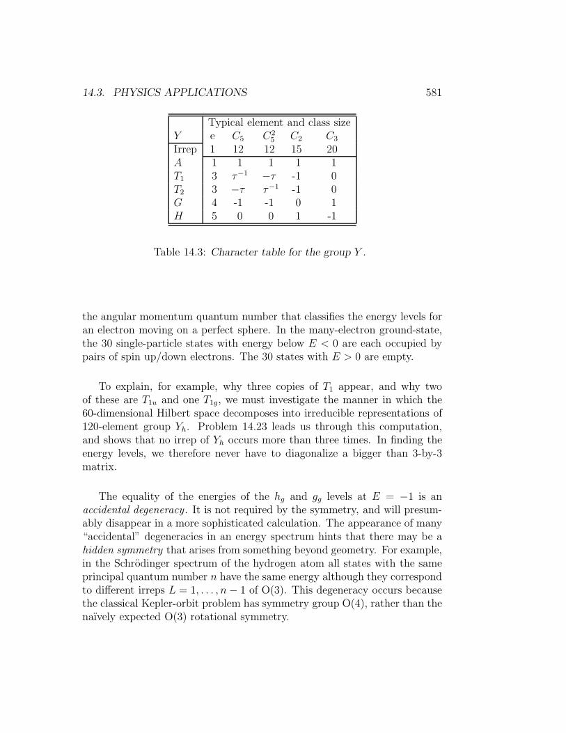
14.3. PHYSICS APPLICATIONS 581
Typical element and class sizeY e C5 C2
5 C2 C3
Irrep 1 12 12 15 20A 1 1 1 1 1T1 3 τ−1 −τ -1 0T2 3 −τ τ−1 -1 0G 4 -1 -1 0 1H 5 0 0 1 -1
Table 14.3: Character table for the group Y .
the angular momentum quantum number that classifies the energy levels foran electron moving on a perfect sphere. In the many-electron ground-state,the 30 single-particle states with energy below E < 0 are each occupied bypairs of spin up/down electrons. The 30 states with E > 0 are empty.
To explain, for example, why three copies of T1 appear, and why twoof these are T1u and one T1g, we must investigate the manner in which the60-dimensional Hilbert space decomposes into irreducible representations of120-element group Yh. Problem 14.23 leads us through this computation,and shows that no irrep of Yh occurs more than three times. In finding theenergy levels, we therefore never have to diagonalize a bigger than 3-by-3matrix.
The equality of the energies of the hg and gg levels at E = −1 is anaccidental degeneracy . It is not required by the symmetry, and will presum-ably disappear in a more sophisticated calculation. The appearance of many“accidental” degeneracies in an energy spectrum hints that there may be ahidden symmetry that arises from something beyond geometry. For example,in the Schrodinger spectrum of the hydrogen atom all states with the sameprincipal quantum number n have the same energy although they correspondto different irreps L = 1, . . . , n− 1 of O(3). This degeneracy occurs becausethe classical Kepler-orbit problem has symmetry group O(4), rather than thenaıvely expected O(3) rotational symmetry.
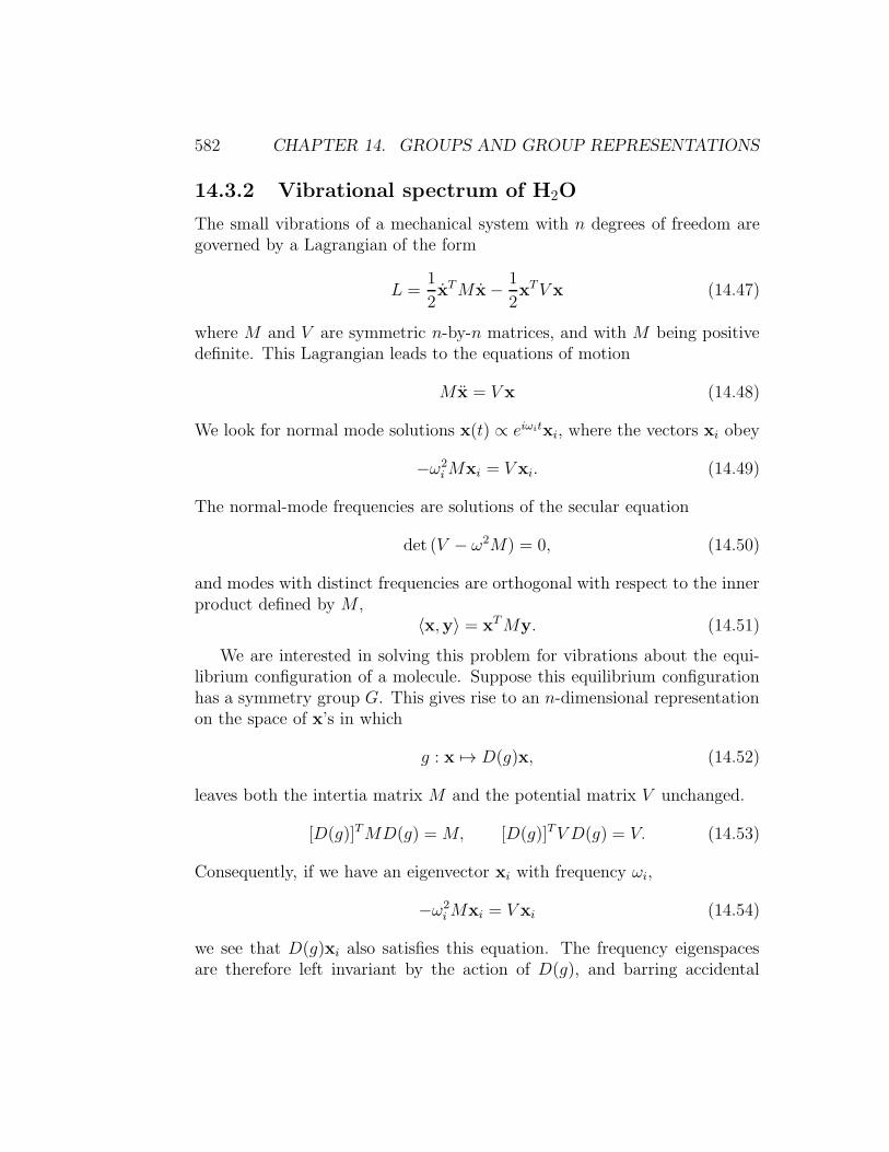
582 CHAPTER 14. GROUPS AND GROUP REPRESENTATIONS
14.3.2 Vibrational spectrum of H2O
The small vibrations of a mechanical system with n degrees of freedom aregoverned by a Lagrangian of the form
L =1
2xTM x− 1
2xTV x (14.47)
where M and V are symmetric n-by-n matrices, and with M being positivedefinite. This Lagrangian leads to the equations of motion
M x = V x (14.48)
We look for normal mode solutions x(t) ∝ eiωitxi, where the vectors xi obey
−ω2iMxi = V xi. (14.49)
The normal-mode frequencies are solutions of the secular equation
det (V − ω2M) = 0, (14.50)
and modes with distinct frequencies are orthogonal with respect to the innerproduct defined by M ,
〈x,y〉 = xTMy. (14.51)
We are interested in solving this problem for vibrations about the equi-librium configuration of a molecule. Suppose this equilibrium configurationhas a symmetry group G. This gives rise to an n-dimensional representationon the space of x’s in which
g : x 7→ D(g)x, (14.52)
leaves both the intertia matrix M and the potential matrix V unchanged.
[D(g)]TMD(g) =M, [D(g)]TV D(g) = V. (14.53)
Consequently, if we have an eigenvector xi with frequency ωi,
−ω2iMxi = V xi (14.54)
we see that D(g)xi also satisfies this equation. The frequency eigenspacesare therefore left invariant by the action of D(g), and barring accidental

14.3. PHYSICS APPLICATIONS 583
degeneracy, there will be a one-to-one correspondence between the frequencyeigenspaces and the irreducible representations occurring in D(g).
Consider, for example, the vibrational modes of the water molecule H2O.This familiar molecule has symmetry group C2v which is generated by twoelements: a rotation a through π about an axis through the oxygen atom,and a reflection b in the plane through the oxygen atom and bisecting theangle between the two hydrogens. The product ab is a reflection in the planedefined by the equilibrium position of the three atoms. The relations area2 = b2 = (ab)2 = e, and the characters are displayed in table 14.4.
class and sizeC2v e a b abIrrep 1 1 1 1A1 1 1 1 1A2 1 1 -1 -1B1 1 -1 1 -1B2 1 -1 -1 1
Table 14.4: Character table of C2v.
The group C2v is Abelian, so all the representations are one dimensional.
To find out what representations occur when C2v acts, we need to findthe character of its action D(g) on the nine-dimensional vector
x = (xO, yO, zO, xH1, yH1
, zH1, xH2
, yH2, zH2
). (14.55)
Here the coordinates xH2, yH2
, zH2etc. denote the displacements of the la-
belled atom from its equilibrium position.
We take the molecule as lying in the xy plane, with the z pointing towardsus.

584 CHAPTER 14. GROUPS AND GROUP REPRESENTATIONS
HH1 2
O
H
H
2
2
y
x
x
y
x
yH
H
1
1
O
O
Figure 14.4: Water Molecule.
The effect of the symmetry operations on the atomic displacements is
D(a)x = (−xO,+yO,−zO,−xH2,+yH2
,−zH2,−xH1
,+yH1,−zH1
)
D(b)x = (−xO,+yO,+zO,−xH2,+yH2
,+zH2,−xH1
,+yH1,+zH1
)
D(ab)x = (+xO,+yO,−zO,+xH1,+yH1
,−zH1,+xH2
,+yH2,−zH2
).
Notice how the transformations D(a), D(b) have interchanged the displace-ment co-ordinates of the two hydrogen atoms. In calculating the characterof a transformation we need look only at the effect on atoms that are leftfixed — those that are moved have matrix elements only in non-diagonalpositions. Thus, when computing the compound characters for a b, we canfocus on the oxygen atom. For ab we need to look at all three atoms. Wefind
χD(e) = 9,
χD(a) = −1 + 1− 1 = −1,χD(b) = −1 + 1 + 1 = 1,
χD(ab) = 1 + 1− 1 + 1 + 1− 1 + 1 + 1− 1 = 3.
By using the orthogonality relations, we find the decomposition
9−113
= 3
1111
+
11−1−1
+ 2
1−11−1
+ 3
1−1−11
(14.56)
orχD = 3χA1 + χA2 + 2χB1 + 3χB2. (14.57)

14.3. PHYSICS APPLICATIONS 585
Thus, the nine-dimensional representation decomposes as
D = 3A1 ⊕A2 ⊕ 2B1 ⊕ 3B2. (14.58)
How do we exploit this? First we cut out the junk. Out of the ninemodes, six correspond to easily identified zero-frequency motions – three oftranslation and three rotations. A translation in the x direction would havexO = xH1
= xH2= ξ, all other entries being zero. This displacement vector
changes sign under both a and b, but is left fixed by ab. This behaviouris characteristic of the representation B2. Similarly we can identify A1 astranslation in y, and B1 as translation in z. A rotation about the y axismakes zH1
= −zH2= φ. This is left fixed by a, but changes sign under b and
ab, so the y rotation mode is A2. Similarly, rotations about the x and z axescorrespond to B1 and B2 respectively. All that is left for genuine vibrationalmodes is 2A1 ⊕ B2.
We now apply the projection operator
PA1 =1
4[(χA1(e))∗D(e) + (χA1(a))∗D(b) + (χA1(b))∗D(b) + (χA1(ab))∗D(ab)]
(14.59)to vH1,x, a small displacement of H1 in the x direction. We find
PA1vH1,x =1
4(vH1,x − vH2,x − vH2,x + vH1,x)
=1
2(vH1,x − vH2,x). (14.60)
This mode is an eigenvector for the vibration problem.If we apply PA1 to vH1,y and vO,y we find
PA1vH1,y =1
2(vH1,y + vH2,y),
PA1vO,y = vO,y, (14.61)
but we are not quite done. These modes are contaminated by the y trans-lation direction zero mode, which is also in an A1 representation. Afterwe make our modes orthogonal to this, there is only one left, and this hasyH1
= yH2= −yOmO/(2mH) = a1, all other components vanishing.
We can similarly find vectors corresponding to B2 as
PB2vH1,x =1
2(vH1,x + vH2,x)

586 CHAPTER 14. GROUPS AND GROUP REPRESENTATIONS
PB2vH1,y =1
2(vH1,y − vH2,y)
PB2vO,x = vO,x
and these need to be cleared of both translations in the x direction androtations about the z axis, both of which transform under B2. Again thereis only one mode left and it is
yH1= −yH2
= αxH1= αxH2
= βx0 = a2 (14.62)
where α is chosen to ensure that there is no angular momentum about O,and β to make the total x linear momentum vanish. We have thereforefound three true vibration eigenmodes, two transforming under A1 and oneunder B2 as advertised earlier. The eigenfrequencies, of course, depend onthe details of the spring constants, but now that we have the eigenvectors wecan just plug them in to find these.
14.3.3 Crystal Field Splittings
A quantum mechanical system has a symmetry G if the hamiltonian H obeys
D−1(g)HD(g) = H, (14.63)
for some group action D(g) : H → H on the Hilbert space. If follows thatthe eigenspaces, Hλ, of states with a common eigenvalue, λ, are invariantsubspaces for the representation D(g).
We often need to understand how a degeneracy is lifted by perturbationsthat break G down to a smaller subgroup H . An n-dimensional irreduciblerepresentation of G is automatically a representation of any subgroup of G,but in general it is no longer be irreducible. Thus the n-fold degeneratelevel is split into multiplets, one for each of the irreducible representationsof H contained in the original representation. The manner in which an orig-inally irreducible representation decomposes under restriction to a subgroupis known as the branching rule for the representation.
A physically important case is given by the breaking of the full SO(3)rotation symmetry of an isolated atomic hamiltonian by a crystal field Sup-pose the crystal has octohedral symmetry. The characters of the octohedralgroup are displayed in table 14.5.

14.3. PHYSICS APPLICATIONS 587
Class(size)O e C3(8) C2
4 (3) C2(6) C4(6)A1 1 1 1 1 1A2 1 1 1 -1 -1E 2 -1 2 0 0F2 3 0 -1 1 -1F1 3 0 -1 -1 1
Table 14.5: Character table of the octohedral group O.
The classes are lableled by the rotation angles, C2 being a twofold rotationaxis (θ = π), C3 a threefold axis (θ = 2π/3), etc..
The chacter of the J = l representation of SO(3) is
χl(θ) =sin(2l + 1)θ/2
sin θ/2, (14.64)
and the first few χl’s evaluated on the rotation angles of the classes of O aredsiplayed in table 14.6.
Class(size)l e C3(8) C2
4 (3) C2(6) C4(6)0 1 1 1 1 11 3 0 -1 -1 -12 5 -1 1 1 -13 7 1 -1 -1 -14 9 0 1 1 1
Table 14.6: Characters evaluated on rotation classes
The 9-fold degenerate l = 4 multiplet therefore decomposes as
90111
=
11111
+
2−1200
+
30−1−11
+
30−11−1
, (14.65)

588 CHAPTER 14. GROUPS AND GROUP REPRESENTATIONS
orχ4SO(3) = χA1 + χE + χF1 + χF2 . (14.66)
The octohedral crystal field splits the nine states into four multiplets withsymmetries A1, E, F1, F2 and degeneracies 1, 2, 3 and 3, respectively.
We have considered only the simplest case here, ignoring the complica-tions introduced by reflection symmetries, and by 2-valued spinor represen-tations of the rotation group.
14.4 Further Exercises and Problems
We begin with some technologically important applications of group theoryto cryptography and number theory.
Exercise 14.18: The set Zn forms a group under multiplication only when n isa prime number. Show, however, that the subset U(Zn) ⊂ Zn of elements ofZn that are co-prime to n is a group. It is the group of units of the ring Zn.
Exercise 14.19: Cyclic groups. A group G is said to be cyclic if its elementsconsist of powers an of of an element a, called the generator . The group willbe of finite order |G| = m if am = a0 = e for some m ∈ Z+.
a) Show that a group of prime order is necessarily cyclic, and that anyelement other than the identity can serve as its generator. (Hint: Leta be any element other than e and consider the subgroup consisting ofpowers am.)
b) Show that any subgroup of a cyclic group is itself cyclic.
Exercise 14.20: Cyclic groups and cryptography. In a large cyclic group Git can be relatively easy to compute ax, but to recover x given h = ax onemight have to compute ay and compare it with h for every 1 < y < |G|. If|G| has several hundred digits, such a brute force search could take longerthan the age of the universe. Rather more efficient algorithms for this discretelogarithm problem exist, but the difficulty is still sufficient for it to be usefulin cryptopgraphy.
a) Diffie-Hellman key exchange. This algorithm allows Alice and Bob toestablish a secret key that can be used with a conventional cypher with-out Eve, who is listening to their conversation, being able to reconstructit. Alice choses a random element g ∈ G and an integer x between 1 and|G| and computes gx. She sends g and gx to Bob, but keeps x to herself.

14.4. FURTHER EXERCISES AND PROBLEMS 589
Bob chooses an integer y and computes gy and gxy = (gx)y. He keepsy secret and sends gy to Alice, who computes gxy = (gy)x. Show that,although Eve knows g, gy and gx, she cannot obtain Alice and Bob’ssecret key gxy without solving the discrete logarithm problem.
b) ElGamal public key encryption. This algorithm, based on Diffie-Hellman,was invented by the Egyptian cryptographer Taher Elgamal. It is acomponent of PGP and and other modern encryption packages. To useit, Alice first chooses a random integer x in the range 1 to |G| andcomputes h = ax. She publishes a description of G, together with theelements h and a, as her public key. She keeps the integer x secret. Tosend a message m to Alice, Bob chooses an integer y in the same rangeand computes c1 = ay, c2 = mhy. He transmits c1 and c2 to Alice, butkeeps y secret. Alice can recover m from c1, c2 by computing c2(c
x1)
−1.Show that, although Eve knows Alice’s public key and has overheard c1and c2, she nonetheless cannot decrypt the message without solving thediscrete logarithm problem.
Popular choices for G are subgroups of (Zp)×, for large prime p. (Zp)× is itselfcyclic (can you prove this?), but is unsuitable for technical reasons.
Exercise 14.21: Modular arithmetic and number theory . An integer a is saidto be a quadratic residue mod p if there is an r such that a = r2 (mod p).Let p be an odd prime. Show that if r21 = r22 (mod p) then r1 = ±r2 (mod p),and that r 6= −r (mod p). Deduce that exactly one half of the p− 1 non-zeroelements of Zp are quadratic residues.
Now consider the Legendre symbol
(a
p
)def=
0, a = 0,1, a a quadratic residue (mod p),−1 a not a quadratic residue (mod p).
Show that (a
p
)(b
p
)=
(ab
p
),
and so the Legendre symbol forms a one-dimensional representation of themultiplicative group (Zp)×. Combine this fact with the character orthogonalitytheorem to give an alternative proof that precisely half the p − 1 elements of(Zp)× are quadratic residues. (Hint: To show that the product of two non-residues is a residue, observe that the set of residues is a normal subgroup of(Zp)×, and consider the multiplication table of the resulting quotient group.)

590 CHAPTER 14. GROUPS AND GROUP REPRESENTATIONS
Exercise 14.22: More practice with modular arithmetic. Again let p be anodd prime. Prove Euler’s theorem that
a(p−1)/2 (mod p) =
(a
p
).
(Hint: Begin by showing that the usual school-algebra proof that an equa-tion of degree n can have no more than n solutions remains valid for arith-metic modulo a prime number, and so a(p−1)/2 = 1 (mod p) can have no morethan(p− 1)/2 roots. Cite Fermat’s little theorem to show that these rootsmust be the quadratic residues. Cite Fermat again to show that the quadraticnon-residues must then have a(p−1)/2 = −1 (mod p).)
The harder-to-prove law of quadratic reciprocity asserts that for p, q odd primes,we have
(−1)(p−1)(q−1)/4
(p
q
)=
(q
p
).
Problem 14.23: Buckyball spectrum. Consider the symmetry group of the C60
buckyball molecule of figure 14.3.
a) Starting from the character table of the orientation-preserving icosohe-dral group Y (table 14.3), and using the fact that the Z2 parity inversionσ : r → −r combines with g ∈ Y so that DJg(σg) = DJg(g), whilstDJu(σg) = −DJu(g), write down the character table of the extendedgroup Yh = Y ×Z2 that acts as a symmetry on the C60 molecule. Thereare now ten conjugacy classes, and the ten representations will be la-belled Ag, Au, etc. Verify that your character table has the expectedrow-orthogonality properties.
b) By counting the number of atoms left fixed by each group operation,compute the compound character of the action of Yh on the C60 molecule.(Hint: Examine the pattern of panels on a regulation soccer ball, anddeduce that four carbon atoms are left unmoved by operations in theclass σC2.)
c) Use your compound character from part b), to show that the 60-dimensionalHillbert space decomposes as
HC60= Ag ⊕ T1g ⊕ 2T1u ⊕ T2g ⊕ 2T2u ⊕ 2Gg ⊕ 2Gu ⊕ 3Hg ⊕ 2Hu,
consistent with the energy-levels sketched in figure 14.3.
Problem 14.24: The Frobenius-Schur Indicator. Recall that a real or pseudo-real representation is one such that D(g) ∼ D∗(g), and for unitary matrices D
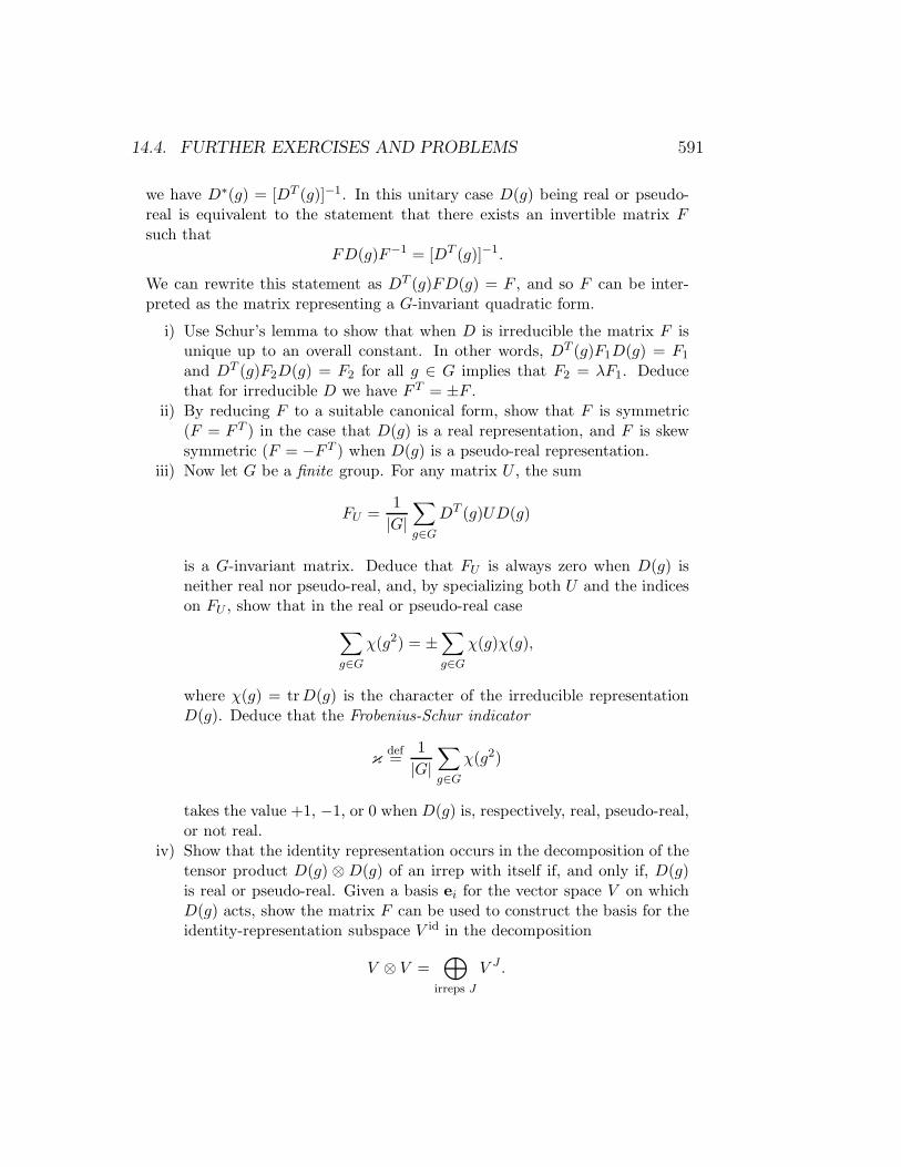
14.4. FURTHER EXERCISES AND PROBLEMS 591
we have D∗(g) = [DT (g)]−1. In this unitary case D(g) being real or pseudo-real is equivalent to the statement that there exists an invertible matrix Fsuch that
FD(g)F−1 = [DT (g)]−1.
We can rewrite this statement as DT (g)FD(g) = F , and so F can be inter-preted as the matrix representing a G-invariant quadratic form.
i) Use Schur’s lemma to show that when D is irreducible the matrix F isunique up to an overall constant. In other words, DT (g)F1D(g) = F1
and DT (g)F2D(g) = F2 for all g ∈ G implies that F2 = λF1. Deducethat for irreducible D we have F T = ±F .
ii) By reducing F to a suitable canonical form, show that F is symmetric(F = F T ) in the case that D(g) is a real representation, and F is skewsymmetric (F = −F T ) when D(g) is a pseudo-real representation.
iii) Now let G be a finite group. For any matrix U , the sum
FU =1
|G|∑
g∈GDT (g)UD(g)
is a G-invariant matrix. Deduce that FU is always zero when D(g) isneither real nor pseudo-real, and, by specializing both U and the indiceson FU , show that in the real or pseudo-real case
∑
g∈Gχ(g2) = ±
∑
g∈Gχ(g)χ(g),
where χ(g) = trD(g) is the character of the irreducible representationD(g). Deduce that the Frobenius-Schur indicator
κdef=
1
|G|∑
g∈Gχ(g2)
takes the value +1, −1, or 0 when D(g) is, respectively, real, pseudo-real,or not real.
iv) Show that the identity representation occurs in the decomposition of thetensor product D(g) ⊗D(g) of an irrep with itself if, and only if, D(g)is real or pseudo-real. Given a basis ei for the vector space V on whichD(g) acts, show the matrix F can be used to construct the basis for theidentity-representation subspace V id in the decomposition
V ⊗ V =⊕
irreps J
V J .

592 CHAPTER 14. GROUPS AND GROUP REPRESENTATIONS
Problem 14.25: Induced Representations. Suppose we know a representationDW (h) : W → W for a subgroup H ⊂ G. From this representation we canconstruct an induced representation IndGH(D
W ) for the larger group G. Theconstruction cleverly combines the coset space G/H with the representationspace W to make a (usually reducible) representation space IndGH(W ) of di-mension |G/H| × dimW .
Recall that there is a natural action of G on the coset space G/H. If x =g1, g2, . . . ∈ G/H then gx is the coset gg1, gg2, . . .. We select from eachcoset x ∈ G/H a representative element ax, and observe that the product gaxcan be decomposed as gax = agxh, where agx is the selected representativefrom the coset gx and h is some element of H. Next we introduce a basis|n, x〉 for IndGH(W ). We use the symbol “0” to label the coset e, and take|n, 0〉 to be the basis vectors for W . For h ∈ H we can therefore set
D(h)|n, 0〉 def= |m, 0〉DWmn(h).
We also define the result of the action of ax on |n, 0〉 to be the vector |n, x〉:
D(ax)|n, 0〉 def= |n, x〉.
We may now obtain the the action of a general element of G on the vectors|n, x〉 by requiring D(g) to be representation, and so computing
D(g)|n, x〉 = D(g)D(ax)|n, 0〉= D(gax)|n, 0〉= D(agxh)|n, 0〉= D(agx)D(h)|n, 0〉= D(agx)|m, 0〉DW
mn(h)
= |m, gx〉DWmn(h).
i) Confirm that the action D(g)|n, x〉 = |m, gx〉DWmn(h), with h obtained
from g and x via the decomposition gax = agxh, does indeed define arepresentation of G. Show also that if we set |f〉 = ∑
n,x fn(x)|n, x〉,then the action of g on the components takes
fn(x) 7→ DWnm(h)fm(g
−1x).
ii) Let f(h) be a class function on H. Let us extend it to a function on Gby setting f(g) = 0 if g /∈ H, and define
IndGH [f ](s) =1
|H|∑
g∈Gf(g−1sg).

14.4. FURTHER EXERCISES AND PROBLEMS 593
Show that IndGH [f ](s) is a class function on G, and further show that ifχW is the character of the starting representation for H then IndGH [χW ]is the character of the induced representation of G. (Hint, only fixedpoints of the G-action on G/H contribute to the character, and gx = xmeans that gax = axh. Thus D
W (h) = DW (a−1x gax).)
iii) Given a representation DV (g) : V → V of G we can trivially obtain a(generally reducible) representation ResGH(V ) of H ⊂ G by restricting Gto H. Define the usual inner product on the group functions by
〈φ1, φ2〉G =1
|G|∑
g∈Gφ1(g
−1)φ2(g),
and show that if ψ is a class function on H and φ a class function on Gthen
〈ψ,ResGH [φ]〉H = 〈IndGH [ψ], φ〉G.Thus, IndGH and ResGH are, in some sense, adjoint operations. Mathe-maticians would call them a pair of mutually adjoint functors.
iv) By applying the result from part (iii) to the characters of the irreduciblerepresentations of G and H, deduce Frobenius’ reciprocity theorem: Thenumber of times an irrepDJ(g) of G occurs in the representation inducedfrom an irrepDK(h) ofH is equal to the number of times that DK occursin the decomposition of DJ into irreps of H.
The representation of the Poincare group (= the SO(1, 3) Lorentz group to-gether with space-time translations) that classifies the states of a spin-J ele-mentary particle are those induced from the spin-J representation of its SO(3)rotation subgroup. The quantum state of a mass m elementary particle istherefore of the form |k, σ〉 where k is the particle’s four-momentum, whichlies is the coset SO(1, 3)/SO(3), and σ is the label from the |J, σ〉 spin state.

594 CHAPTER 14. GROUPS AND GROUP REPRESENTATIONS

Chapter 15
Lie Groups
A Lie group is a group which is also a smooth manifold G. The groupoperation of multiplication (g1, g2) 7→ g3 is required to be a smooth function,as is the operation of taking the inverse of a group element. Lie groups arenamed after the Norwegian mathematician Sophus Lie. The examples mostcommonly met in physics are the infinite families of matrix groups GL(n),SL(n), O(n), SO(n), U(n), SU(n), and Sp(n), all of which we shall describein this chapter, togther with the family of five exceptional Lie groups: G2,F4, E6, E7, and E8, which have applications in string theory.
One of the properties of a Lie group is that, considered as a manifold,the neighbourhood of any point looks exactly like that of any other. Accord-ingly, the group’s dimension and much of its structure can be understood byexamining the immediate vicinity any chosen point, which we may as welltake to be the identity element. The vectors lying in the tangent space atthe identity element make up the Lie algebra of the group. Computations inthe Lie algebra are often easier than those in the group, and provide much ofthe same information. This chapter will be devoted to studying the interplaybetween the Lie group itself and this Lie algebra of infinitesimal elements.
15.1 Matrix Groups
The Classical Groups are described in a book with this title by HermannWeyl. They are subgroups of the general linear group, GL(n,F), which con-sists of invertible n-by-n matrices over the field F. We will mostly considerthe cases F = C or F = R.
595

596 CHAPTER 15. LIE GROUPS
A near-identity matrix in GL(n,R) can be written g = I + ǫA, where Ais an arbitrary n-by-n real matrix. This matrix contains n2 real entries, sowe can move away from the identity in n2 distinct directions. The tangentspace at the identity, and hence the group manifold itself, is therefore n2
dimensional. The manifold of GL(n,C) has n2 complex dimensions, and thiscorresponds to 2n2 real dimensions.
If we restrict the determinant of a GL(n,F) matrix to be unity, we getthe special linear group, SL(n,F). An element near the identity in this groupcan still be written as g = I + ǫA, but since
det (I + ǫA) = 1 + ǫ tr(A) +O(ǫ2), (15.1)
this requires tr(A) = 0. The restriction on the trace means that SL(n,R)has dimension n2 − 1.
15.1.1 The Unitary and Orthogonal Groups
Perhaps the most important of the matrix groups are the unitary and or-thogonal groups.
The Unitary group
The unitary group U(n) comprises the set of n-by-n complex matrices U suchthat U † = U−1. If we consider matrices near the identity
U = I + ǫA, (15.2)
with ǫ real, then unitarity requires
I +O(ǫ2) = (I + ǫA)(I + ǫA†)
= I + ǫ(A + A†) +O(ǫ2), (15.3)
so Aij = −(Aji)∗ —it i.e. A is skew hermitian. A complex skew-hermitianmatrix contains
n +
[2× 1
2n(n− 1)
]= n2
real parameters. In this counting, the first “n” is the number of entries onthe diagonal, each of which must be of the form i times a real number. Then(n− 1)/2 is the number of entries above the main diagonal, each of which

15.1. MATRIX GROUPS 597
can be an arbitrary complex number. The number of real dimensions in thegroup manifold is therefore n2. As U †U = I, the rows or columns in thematrix U form an orthonormal set of vectors. Their entries are thereforebounded, |Uij| ≤ 1, and this property leads to the n2 dimensional groupmanifold of U(n) being a compact set.
When a group manifold is compact, we say that the group itself is acompact group. There is a natural notion of volume on a group manifoldand compact Lie groups have finite total volume. Because of this, they havemany properties in common with the finite groups we studied in the previouschapter.
Recall that a group is simple if it possesses no invariant subgroups. U(n)is not simple. Its centre Z is an invariant U(1) subgroup consisting of matricesof the form U = eiθ I. The special unitary group SU(n), consists of n-by-n unimodular (having determinant +1) unitary matrices. It is not strictlysimple because its center Z consists of the discrete subgroup of matricesUm = ωm I with ω an n-th root of unity, and this is an invariant subgroup.Because the centre, its only invariant subgroup, is not a continuous group,SU(n) is counted as being simple in Lie theory. With U = I + ǫA, as above,the unimodularity imposes the additional constraint on A that trA = 0, sothe SU(n) group manifold is n2 − 1 dimensional.
The orthogonal group
The orthogonal group O(n) consists of the the set of real matrices O with theproperty that OT = O−1. For a matrix in the neighbourhood of the identity,O = I + ǫA, this property requires that A be skew symmetric: Aij = −Aij .Skew symmetric real matrices have n(n−1)/2 independent entries, and so thegroup manifold of O(n) is n(n− 1)/2 dimensional. The condition OTO = Imeans that the rows or columns of O, considered as row or column vectors,are orthonormal. All entries are bounded, i.e. |Oij| ≤ 1, and again this leadsto O(n) being a compact group.
The identity
1 = det (OTO) = detOTdetO = (detO)2 (15.4)
tells us that detO = ±1. The subset of orthogonal matrices with detO = +1constitute a subgroup of O(n) called the special orthogonal group SO(n). Theunimodularity condition discards a disconnected part of the group manifoldand does not reduce its dimension, which remains n(n− 1)/2.
598 CHAPTER 15. LIE GROUPS
15.1.2 Symplectic Groups
The symplectic groups (named from the Greek, meaning to “fold together”)are perhaps less familiar than the other matrix groups.
We start with a non-degenerate skew-symmetric matrix ω. The symplec-tic group Sp(2n,F) is then defined by
Sp(2n,F) = S ∈ GL(2n,F) : STωS = ω. (15.5)
Here F can be R or C. When F = C, we still use the transpose “T ,” notthe adjoint “†,” in this definition. Setting S = I2n+ ǫA and demanding thatSTωS = ω shows that ATω + ωA = 0.
It does not matter what skew matrix ω we start from, because we canalways find a basis in which ω takes its canonical form:
ω =
(0 −InIn 0
). (15.6)
In this basis we find, after a short computation, that the most general formfor A is
A =
(a bc −aT
). (15.7)
Here, a is any n-by-n matrix, and b and c are symmetric (i.e. bT = b andcT = c) n-by-n matrices. If the matrices are real, then counting the degreesof freedom gives the dimension of the real symplectic group as
dimSp(2n,R) = n2 +[2× n
2(n+ 1)
]= n(2n+ 1). (15.8)
The entries in a, b, c can be arbitrarily large. Sp(2n,R) is not compact.The determinant of any symplectic matrix is +1. To see this take the
elements of ω to be ωij, and let
ω(x, y) = ωijxiyj (15.9)
be the associated skew bilinear (not sesquilinear) form . Then Weyl’s identityfrom exercise A.19 shows that
Pf (ω) (detM) det |x1, . . . , x2n|=
1
2nn!
∑
π∈S2n
sgn (π)ω(Mxπ(1),Mxπ(2)) · · ·ω(Mxπ(2n−1),Mxπ(2n)),
15.1. MATRIX GROUPS 599
for any linear map M . If ω(x, y) = ω(Mx,My), we conclude that detM =1 — but preserving ω is exactly the condition that M be an element ofthe symplectic group. Since the matrices in Sp(2n,F) are automaticallyunimodular there is no “special symplectic” group.
Unitary symplectic group
The intersection of two groups is also a group. We therefore define the unitarysymplectic group as
Sp(n) = Sp(2n,C) ∩U(2n). (15.10)
This group is compact — a property in inherits from the compactness of theU(n) in which it is embedded as a subgroup. We will see that its dimensionis n(2n + 1), the same as the non-compact Sp(2n,R). Sp(n) may also bedefined as U(n,H) where H denotes the skew field of quaternions.Warning: Physics papers often make no distinction between Sp(n), whichis a compact group, and Sp(2n,R) which is non-compact. To add to theconfusion the compact Sp(n) is also sometimes called Sp(2n). You have tojudge from the context what group the author has in mind.Physics Application: Kramers’ degeneracy.
Let σi be the Pauli matrices, and L the orbital angular momentum oper-ator. The matrix C = iσ2 has the property that
C−1σiC = −σ∗i . (15.11)
A time-reversal invariant Hamiltonian containing L ·S spin-orbit interactionsobeys
C−1HC = H∗. (15.12)
We regard the 2n-by-2n matrix H as being an n-by-n matrix whose entriesHij are themselves 2-by-2 matrices. We therefore expand these entries as
Hij = h0ij + i3∑
n=1
hnij σn.
The condition (15.12) now implies that the haij are real numbers. We thereforesay that H is real quaternionic. This is because the Pauli sigma matrices arealgebraically isomorphic to Hamilton’s quaternions under the identification
iσ1 ↔ i,iσ2 ↔ j,iσ3 ↔ k.
(15.13)

600 CHAPTER 15. LIE GROUPS
The hermiticity of H requires that Hji = H ij where the overbar denotesquaternionic conjugation, i.e. the mapping
q0 + iq1σ1 + iq2σ2 + iq3σ3 → q0 − iq1σ1 − iq2σ2 − iq3σ3. (15.14)
If Hψ = Eψ, then HCψ∗ = Eψ∗. Since C is skew, ψ and Cψ∗ are necessarilyorthogonal. Therefore all states are doubly degenerate. This is Kramers’degeneracy.
H may be diagonalized by a matrix in U(n,H), where U(n,H) consistsof those elements of U(2n) that satisfy C−1UC = U∗. We may rewrite thiscondition as
C−1UC = U∗ ⇒ UCUT = C,
so U(n,H) consists of the unitary matrices that preserve the skew symmet-ric matrix C. Thus U(n,H) ⊆ Sp(n). Further investigation shows thatU(n,H) = Sp(n).
We can exploit the quaternionic viewpoint to count the dimensions. LetU = I+ǫB be in U(n,H). Then Bij+Bji = 0. The diagonal elements of B arethus pure “imaginary” quaternions having no part proportional to I. Thereare therefore 3 parameters for each diagonal element. The upper triangle hasn(n− 1)/2 independent elements, each with 4 parameters. Counting up, wefind
dimU(n,H) = dimSp(n) = 3n+[4× n
2(n− 1)
]= n(2n+ 1). (15.15)
Thus, as promised, we see that the compact group Sp(n) and the non-compact group Sp(2n,R) have the same dimension.
We can also count the dimension of Sp(n) by looking at our previousmatrices
A =
(a bc −aT
)
where a b and c are now allowed to be complex, but with the restriction thatS = I + ǫA be unitary. This requires A to be skew-hermitian, so a = −a†,and c = −b†, while b (and hence c) remains symmetric. There are n2 freereal parameters in a, and n(n + 1) in b, so
dimSp(n) = (n2) + n(n + 1) = n(2n+ 1),
as before.

15.2. GEOMETRY OF SU(2) 601
Exercise 15.1: Show that
SO(2N) ∩ Sp(2N,R) ∼= U(N).
Hint: Group the 2N basis vectors on which O(2N) acts into pairs xn and yn,n = 1, . . . , N . Assemble these pairs into zn = xn + iyn and z = xn − iyn. Letω be the linear map that takes xn → yn and yn → −xn. Show that the subsetof SO(2N) that commutes with ω mixes zi’s only with zi’s and zi’s only withzi’s.
15.2 Geometry of SU(2)
To get a sense of Lie groups as geometric objects, we will study the simplestnon-trivial case, SU(2), in some detail.
A general 2-by-2 complex matrix can be parametrized as
U =
(x0 + ix3 ix1 + x2
ix1 − x2 x0 − ix3). (15.16)
The determinant of this matrix is unity, provided
(x0)2 + (x1)2 + (x2)2 + (x3)2 = 1. (15.17)
When this condition is met, and if in addition the xi are real, the matrix isunitary: U † = U−1. The group manifold of SU(2) can therefore be identifiedwith the three-sphere S3. We will take as local co-ordinates x1, x2, x3. Whenwe desire to know x0 we will find it from x0 =
√1− (x1)2 − (x2)2 − (x3)2.
This co-ordinate chart only labels the points in the half of the three-spherehaving x0 > 0, but this is typical of any non-trivial manifold. A completeatlas of charts can be constructed if needed.
We can simplify our notation by using the Pauli sigma matrices
σ1 =
(0 11 0
), σ2 =
(0 −ii 0
), σ3 =
(1 00 −1
). (15.18)
These obey
[σi, σj] = 2iǫijkσk, and σiσj + σj σi = 2δijI. (15.19)
In terms of them, we can write the general element of SU(2) as
g = U = x0I + ix1σ1 + ix2σ2 + ix3σ3. (15.20)

602 CHAPTER 15. LIE GROUPS
Elements of the group in the neighbourhood of the identity differ from e ≡ Iby real linear combinations of the iσi. The three-dimensional vector spacespanned by these matrices is therefore the tangent space TGe at the identityelement. For any Lie group, this tangent space is called the Lie algebra,g = LieG of the group. There will be a similar set of matrices iλi for anymatrix group. They are called the generators of the Lie algebra, and satisfycommutation relations of the form
[iλi, iλj ] = −f kij (iλk), (15.21)
or equivalently[λi, λj] = if k
ij λk (15.22)
The f kij are called the structure constants of the algebra. The “i”’s associ-
ated with the λ’s in this expression are conventional in physics texts becausefor quantum mechanics application we usually desire the λi to be hermitian.They are usually absent in books aimed at mathematicians.
Exercise 15.2: Let λ1 and λ2 be hermitian matrices. Show that if we defineλ3 by the relation [λ1, λ2] = iλ3, then λ3 is also a hermitian matrix.
Exercise 15.3: For the group O(n) the matrices “iλ” are real n-by-n skewsymmetric matrices A. Show that if A1 and A2 are real skew symmetricmatrices, then so is [A1, A2].
Exercise 15.4: For the group Sp(2n,R) the iλ matrices are of the form
A =
(a bc −aT
)
where a is any real n-by-n matrix and b and c are symmetric (bT = b andcT = c) real n-by-n matrices. Show that the commutator of any two matricesof this form is also of this form.
15.2.1 Invariant vector fields
Consider a matrix group, and in it a group element I + iǫλi lying close tothe identity e ≡ I. Draw an arrow connecting I to I + iǫλi, and regardthis arrow as a vector Li lying in TGe. Next, map the infinitesimal elementI + iǫλi to the neighbourhood an arbitrary group element g by multiplying
15.2. GEOMETRY OF SU(2) 603
on the left to get g(I + iǫλi). By drawing an arrow from g to g(I + iǫλi), weobtain a vector Li(g) lying in TGg. This vector at g is the push-forward ofthe vector at e by left multiplication by g. For example, consider SU(2) withinfinitesimal element I + iǫσ3. We find
g(I + iǫσ3) = (x0 + ix1σ1 + ix2σ2 + ix3σ3)(I + iǫσ3)
= (x0 − ǫx3) + iσ1(x1 − ǫx2) + iσ2(x
2 + ǫx1) + iσ3(x3 + ǫx0).
(15.23)
This computation can also be interpreted as showing that the multiplicationof g ∈ SU(2) on the right by (I + iǫσ3) displaces the point g, changing its xi
parameters by an amount
δ
x0
x1
x2
x3
= ǫ
−x3−x2x1
x0
. (15.24)
Knowing how the displacement looks in terms of the x1, x2, x3 co-ordinatesystem lets us read off the ∂/∂xµ components of a vector L3 lying in TGg:
L3 = −x2∂1 + x1∂2 + x0∂3. (15.25)
Since g can be any point in the group, we have constructed a globally-definedvector field L3 that acts on a function F (g) on the group manifold as
L3F (g) = limǫ→0
1
ǫ[F (g(I + iǫσ3))− F (g)]
. (15.26)
Similarly, we obtain
L1 = x0∂1 − x3∂2 + x2∂3
L2 = x3∂1 + x0∂2 − x1∂3. (15.27)
The vector fields Li are said to be left invariant because the push-forwardof the vector Li(g) lying in the tangent space at g by multiplication on theleft by any g′ produces a vector g′∗[Li(g)] lying in the tangent space at g′g,and this pushed-forward vector coincides with the Li(g
′g) already there. Wecan express this statement tersely as g∗Li = Li.
604 CHAPTER 15. LIE GROUPS
Using ∂ix0 = −xi/x0, i = 1, 2, 3, we can compute the Lie brackets and
find[L1, L2] = −2L3. (15.28)
In general[Li, Lj] = −2ǫijkLk, (15.29)
which coincides with the matrix commutator of the iσi.This construction works for all Lie groups. For each basis vector Li in the
tangent space at the identity e, we push it forward to the tangent space at gby left multiplication by g, and so construct the global left-invariant vectorfield Li. The Lie bracket of these vector fields will be
[Li, Lj ] = −f kij Lk, (15.30)
where the coefficients f kij are guaranteed to be position independent because
(see exercise 12.5) the operation of taking the Lie bracket of two vector fieldscommutes with the operation of pushing-forward the vector fields. Con-sequently, the Lie bracket at any point is just the image of the Lie bracketcalculated at the identity. When the group is a matrix group, this Lie bracketwill coincide with the commutator of the iλi, that group’s analogue of theiσi matrices.
The Exponential map
Recall that given a vector field X ≡ Xµ∂µ we define associated flow bysolving the equation
dxµ
dt= Xµ(x(t)). (15.31)
If we do this for the left-invariant vector field L, with initial conditionx(0) = e, we obtain a t-dependent group element g(x(t)), which we denoteby Exp (tL). The symbol “Exp ” stands for the exponential map which takeselements of the Lie algebra to elements of the Lie group. The reason for thename and notation is that for matrix groups this operation corresponds tothe usual exponentiation of matrices. Elements of the matrix Lie group aretherefore exponentials of matrices in the the Lie algebra. To see this, supposethat Li is the left invariant vector field derived from iλi. Then the matrix
g(t) = exp(itλi) ≡ I + itλi −1
2t2λ2i − i
1
3!t3λ3i + · · · (15.32)

15.2. GEOMETRY OF SU(2) 605
is an element of the group, and
g(t+ ǫ) = exp(itλi) exp(iǫλi) = g(t)(I + iǫλi +O(ǫ2)
). (15.33)
From this we deduce that
d
dtg(t) = lim
ǫ→0
1
ǫ[g(t)(I + iǫλi)− g(t)]
= Lig(t). (15.34)
Since exp(itλ) = I when t = 0, we deduce that Exp (tLi) = exp(itλi).
Right-invariant vector fields
We can also use multiplication on the right to push forward an infinitesimalgroup element. For example:
(I + iǫσ3)g = (I + iǫσ3)(x0 + ix1σ1 + ix2σ2 + ix3σ3)
= (x0 − ǫx3) + iσ1(x1 + ǫx2) + iσ2(x
2 − ǫx1) + iσ3(x3 + ǫx0).
(15.35)
This motion corresponds to the right-invariant vector field
R3 = x2∂1 − x1∂2 + x0∂3. (15.36)
Similarly, we obtain
R1 = x0∂1 + x3∂2 − x2∂3,R2 = −x3∂1 + x0∂2 + x1∂3, (15.37)
and find that[R1, R2] = +2R3. (15.38)
In general,[Ri, Rj] = +2ǫijkRk. (15.39)
For any Lie group, the Lie brackets of the right-invariant fields will be
[Ri, Rj ] = +fijkRk (15.40)
whenever[Li, Lj] = −fij kLk (15.41)

606 CHAPTER 15. LIE GROUPS
are the Lie brackets of the left-invariant fields. The relative minus sign be-tween the bracket algebra of the left- and right-invariant vector fields hasthe same origin as the relative sign between the commutators of space- andbody-fixed rotations in classical mechanics. Because multiplication from theleft does not interfere with multiplication from the right, the left and rightinvariant fields commute:
[Li, Rj ] = 0. (15.42)
15.2.2 Maurer-Cartan Forms
Suppose that g is an element of a group and dg denotes its exterior derivative.Then the combination dg g−1 is a Lie-algebra-valued one form. For example,starting from the elements of SU(2)
g = x0 + ix1σ1 + ix2σ2 + ix3σ3
g−1 = g† = x0 − ix1σ1 − ix2σ2 − ix3σ3 (15.43)
we compute
dg = dx0 + idx1σ1 + idx2σ2 + idx3σ3
= (x0)−1(−x1dx1 − x2dx2 − x3dx3) + idx1σ1 + idx2σ2 + idx3σ3.
(15.44)
From this we find
dgg−1 = iσ1((x0 + (x1)2/x0)dx1 + (x3 + (x1x2)/x0)dx2 + (−x2 + (x1x3)/x0)dx3
)
+iσ2((−x3 + (x2x1)/x0)dx1 + (x0 + (x2)2/x0)dx2 + (x1 + (x2x3)/x0)dx3
)
+iσ3((x2 + (x3x1)/x0)dx1 + (−x1 + (x3x2)/x0)dx2 + (x0 + (x3)2/x0)dx3
).
(15.45)
Observe that the part proportional to the identity matrix has cancelled. Theresult of inserting a vector X i∂i into dg g
−1 is therefore an element of theLie algebra of SU(2). This is what we mean when we say that dg g−1 isLie-algebra-valued .
For a general group, we define the (right invariant) Maurer-Cartan forms
ωiR as being the coeffecient of the Lie algebra generator iλi. Thus, for SU(2),we have
dgg−1 = ωR = (iσi)ωiR. (15.46)
15.2. GEOMETRY OF SU(2) 607
If we evaluate one-form ω1R on the right invariant vector field R1, we find
ω1R(R1) = (x0 + (x1)2/x0)x0 + (x3 + (x1x2)/x0)x3 + (−x2 + (x1x3)/x0)(−x2)
= (x0)2 + (x1)2 + (x2)2 + (x3)2
= 1. (15.47)
Working similarly, we find
ω1R(R2) = (x0 + (x1)2/x0)(−x3) + (x3 + (x1x2)/x0)x0 + (−x2 + (x1x3)/x0)x1
= 0. (15.48)
In general, we discover that ωiR(Rj) = δij . The Maurer-Cartan forms thereforeconstitute the dual basis to the right-invariant vector fields.
We may similarly define the left-invariant Maurer-Cartan forms by
g−1dg = ωL = (iσi)ωiL. (15.49)
These obey ωiL(Lj) = δij , showing that the ωiL are the dual basis to theleft-invariant vector fields.
Acting with the exterior derivative d on gg−1 = I tells us that d(g−1) =−g−1dgg−1. By exploiting this fact, together with the anti-derivation prop-erty
d(a ∧ b) = da ∧ b+ (−1)pa ∧ db,we may compute the exterior derivative of ωR. We find that
dωR = d(dgg−1) = (dgg−1) ∧ (dgg−1) = ωR ∧ ωR. (15.50)
A matrix product is implicit here. If it were not, the product of the twoidentical 1-forms on the right would automatically be zero. When we makethis matrix structure explicit, we see that
ωR ∧ ωR = ωiR ∧ ωjR(iσi)(iσj)=
1
2ωiR ∧ ωjR [iσi, iσj ]
= −12f kij (iσk)ω
iR ∧ ωjR, (15.51)
so
dωkR = −12f kij ω
iR ∧ ωjR. (15.52)

608 CHAPTER 15. LIE GROUPS
These equations are known as the Maurer-Cartan relations for the right-invariant forms.
For the left-invariant forms we have
dωL = d(g−1dg) = −(g−1dg) ∧ (g−1dg) = −ωL ∧ ωL, (15.53)
or
dωkL = +1
2f kij ω
iL ∧ ωjL. (15.54)
The Maurer-Cartan relations appear in the physics literature when wequantize gauge theories. They are one part of the BRST transformations ofthe Fadeev-Popov ghost fields. We will provide a further discussion of thesetransformations in the next chapter.
15.2.3 Euler Angles
In physics it is common to use Euler angles to parameterize the group SU(2).We can write an arbitrary SU(2) matrix U as a product
U = exp−iφσ3/2 exp−iθσ2/2 exp−iψσ3/2,
=
(e−iφ/2 00 eiφ/2
)(cos θ/2 − sin θ/2sin θ/2 cos θ/2
)(e−iψ/2 0
0 eiψ/2
),
=
(e−i(φ+ψ)/2 cos θ/2 −ei(ψ−φ)/2 sin θ/2ei(φ−ψ)/2 sin θ/2 ei(ψ+φ)/2 cos θ/2
). (15.55)
Comparing with the earlier expression for U in terms of the co-ordinates xµ,we obtain the Euler-angle parameterization of the three-sphere
x0 = cos θ/2 cos(ψ + φ)/2,
x1 = sin θ/2 sin(φ− ψ)/2,x2 = − sin θ/2 cos(φ− ψ)/2,x3 = − cos θ/2 sin(ψ + φ)/2. (15.56)
When the angles are taken in the range 0 ≤ φ < 2π, 0 ≤ θ < π, 0 ≤ ψ < 4πwe cover the entire three-sphere exactly once.
Exercise 15.5: Show that the Hopf map, defined in chapter 3, Hopf : S3 → S2
is the “forgetful” map (θ, φ, ψ) → (θ, φ), where θ and φ are spherical polarco-ordinates on the two-sphere.

15.2. GEOMETRY OF SU(2) 609
Exercise 15.6: Show that
U−1dU = − i2σi Ω
iL,
where
Ω1L = sinψ dθ − sin θ cosψ dφ,
Ω2L = cosψ dθ + sin θ sinψ dφ,
Ω3L = dψ + cos θ dφ.
Observe that these 1-forms are essentially the components
ωX = sinψ θ − sin θ cosψ φ,
ωY = cosψ θ + sin θ sinψ φ,
ωZ = ψ + cos θ φ.
of the angular velocity ω of a body with respect to the body-fixed XY Z axesin the Euler-angle conventions of exercise 11.17.
Similarly, show that
dUU−1 = − i2σi Ω
iR,
where
Ω1R = − sinφdθ + sin θ cosφdψ,
Ω2R = cosφdθ + sin θ sinφdψ,
Ω3R = dφ+ cos θ dψ,
Compute the components ωx, ωy, ωz of the same angular velocity vector ω, butnow taken with respect to the space-fixed xyz frame. Compare your answerwith the ΩiR.
15.2.4 Volume and Metric
The manifold of any Lie group has a natural metric, which is obtained bytransporting the Killing form (see section 15.3.2) from the tangent space atthe identity to any other point g by either left or right multiplication byg. In For a compact group, the resultant left- and right-invariant metricscoincide. In the particular case of SU(2) this metric is the usual metric onthe three-sphere.

610 CHAPTER 15. LIE GROUPS
Using the Euler angle expression for the xµ to compute the dxµ, we canexpress the metric on the sphere as
ds2 = (dx0)2 + (dx1)2 + (dx2)2 + (dx3)2,
=1
4
(dθ2 + cos2θ/2(dψ + dφ)2 + sin2θ/2(dψ − dφ)2
),
=1
4
(dθ2 + dψ2 + dφ2 + 2 cos θ dφ dψ
). (15.57)
Here, to save space, we have used the traditional physics way of writing ametric. In the more formal notation, where we think of the metric as beinga bilinear function, we would write the last line as
g( , ) =1
4(dθ ⊗ dθ + dψ ⊗ dψ + dφ⊗ dφ+ cos θ(dφ⊗ dψ + dψ ⊗ dφ)) .
(15.58)From (15.58) we find
g = det (gµν) =1
43
∣∣∣∣∣∣
1 0 00 1 cos θ0 cos θ 1
∣∣∣∣∣∣
=1
64(1− cos2θ) =
1
64sin2θ. (15.59)
The volume element,√g dθdφdψ, is therefore
d(Volume) =1
8sin θdθdφdψ, (15.60)
and the total volume of the sphere is
Vol(S3) =1
8
∫ π
0
sin θdθ
∫ 2π
0
dφ
∫ 4π
0
dψ = 2π2. (15.61)
This volume coincides, for d = 4, with the standard expression for the volumeof Sd−1, the surface of the d-dimensional unit ball,
Vol(Sd−1) =2πd/2
Γ(d2). (15.62)
Exercise 15.7: Evaluate the Maurer-Cartan form ω3L in terms of the Euler
angle parameterization, and hence show that
iω3L =
1
2tr (σ3U
−1dU) = − i2(dψ + cos θ dφ).

15.2. GEOMETRY OF SU(2) 611
Now recall that the Hopf map takes the point on the three-sphere with Eulerangle co-ordinates (θ, φ, ψ) to the point on the two-sphere with spherical polarco-ordinates (θ, φ). Thus, if we set A = −dψ − cos θ dφ, then we find
F ≡ dA = sin θ dθ dφ = Hopf∗(d[AreaS2
]).
Also observe that
A ∧ F = − sin θ dθ dφ dψ.
From this, show that the Hopf index of the Hopf map itself is equal to
1
16π2
∫
S3
A ∧ F = −1.
Exercise 15.8: Show that for U the defining two-by-two matrices of SU(2), wehave ∫
SU(2)tr[(U−1dU)3
]= 24π2.
Suppose we have a map g : R3 → SU(2) such that g(x) goes to the identityelement at infinity. Consider the integral
S[g] =1
24π2
∫
R3
tr (g−1dg)3,
where the 3-form tr (g−1dg)3 is the pull-back to R3 of the form tr [(U−1dU)3]on SU(2). Show that if we we make the variation g → g + δg, then
δS[g] =1
24π2
∫
R3
d3 tr
((g−1δg)(g−1dg)2
)= 0,
and so S[g] is topological invariant of the map g. Conclude that the functionalS[g] is an integer, that integer being the Brouwer degree, or winding number,of the map g : S3 → S3.
Exercise 15.9: Generalize the result of the previous problem to show, for anymapping x 7→ g(x) into a Lie group G, and for n an odd integer, that then-form tr (g−1dg)n constructed from the Maurer-Cartan form is closed, andthat
δ tr (g−1dg)n = dn tr
((g−1δg)(g−1dg)n−1
).
(Note that for even n the trace of (g−1dg)n vanishes identically.)

612 CHAPTER 15. LIE GROUPS
15.2.5 SO(3) ≃ SU(2)/Z2
The groups SU(2) and SO(3) are locally isomorphic. They have the sameLie algebra, but differ in their global topology. Although rotations in spaceare elements of SO(3), electrons respond to these rotations by transformingunder the two-dimensional defining representation of SU(2). As we shall see,this means that after a rotation through 2π the electron wavefunction comesback to minus itself. The resulting orientation entanglement is characteristicof the spinor representation of rotations and is intimately connected withthe Fermi statistics of the electron. The spin representations were discoveredby Elie Cartan in 1913, some years before they were needed in physics.
The simplest way to motivate the spin/rotation connection is via thePauli sigma matrices. These matrices are hermitian, traceless, and obey
σiσj + σj σi = 2δijI. (15.63)
If, for any U ∈ SU(2), we define
σ′i = UσiU
−1, (15.64)
then the σ′i are also hermitian, traceless, and obey (15.63). Since the original
σi form a basis for the space of hermitian traceless matrices, we must have
σ′i = σjRji (15.65)
for some real 3-by-3 matrix having entries Rij . From (15.63) we find that
2δij = σ′iσ
′j + σ′
j σ′i
= (σlRli)(σmRmj) + (σmRmj)(σlRli)
= (σlσm + σmσl)RliRmj
= 2δlmRliRmj .
ThusRmiRmk = δik. (15.66)
In other words, RTR = I, and so R is an element of O(3). Now the determi-nant of any orthogonal matrix is ±1, but the manifold of SU(2) is a connectedset and R = I when U = I. Since a continuous map from a connected set tothe integers must be a constant, we conclude that detR = 1 for all U . TheR matrices are therefore in SO(3).

15.2. GEOMETRY OF SU(2) 613
We now exploit the principle of the sextant to show that the correspon-dance goes both ways, i.e. we can find a U(R) for any element R ∈ SO(3).
Left−hand half of fixed
hand half is transparant mirror is silvered. Right−
View through telescope of sun brought down to touch horizon
120
9060 30
0o
oo o
o
θ
Pivot
Movable Mirror
2θ
To sun
Telescope
Fixed, half silvered mirror
To Horizon
Figure 15.1: The sextant. The telescope and the half-silvered mirror are fixedto the frame of the instrument, which also holds the scale. The second mirrorand attached pointer pivot so that the angle θ between the mirrors can bevaried and accurately recorded. The scale is calibrated so as to display thealtitude 2θ. For the configuration shown, θ = 15 while the pointer indicatesthat the sun is 30 above the horizon.
This familiar instrument is used to measure the altitude of the sun above thehorizon while standing on the unsteady deck of a ship at sea. A theodolite orsimilar device would be rendered useless by the ship’s pitching and rolling.The sextant exploits the fact that successive reflection in two mirrors inclinedat an angle θ to one another serves to rotate the image through an angle 2θabout the line of intersection of the mirror planes. This rotation is used tosuperimpose the image of the sun onto the image of the horizon, where itstays even if the instrument is rocked back and forth. Exactly the same trickis used in constructing the spinor representations of the rotation group.

614 CHAPTER 15. LIE GROUPS
Consider a vector x with components xi and form the matrix x = xiσi.Now, if n is a unit vector with components ni, then
(−σini)x(σknk) =(xj − 2(n · x)(nj)
)σj = x− 2(n · x)n (15.67)
The vector x−2(n·x)n is the result of reflecting x in the plane perpendicularto n. Consequently
−(σ1 cos θ/2 + σ2 sin θ/2)(−σ1) x (σ1)(σ1 cos θ/2 + σ2 sin θ/2) (15.68)
performs two successive reflections on x. The first, a reflection in the “1”plane, is performed by the inner σ1’s. The second reflection, in a plane atan angle θ/2 to the “1” plane, is performed by the (σ1 cos θ/2+ σ2 sin θ/2)’s.Multiplying out the factors, and using the σi algebra, we find
(cos θ/2− σ1σ2 sin θ/2)x(cos θ/2 + σ1σ2 sin θ/2)
= σ1(cos θ x1 − sin θ x2) + σ2(sin θ x
1 + cos θ x2) + σ3x3. (15.69)
The effect on x is a rotation
x1 7→ cos θ x1 − sin θ x2,
x2 7→ sin θ x1 + cos θ x2,
x3 7→ x3, (15.70)
through the angle θ about the 3 axis. We can drop the xi and re-express(15.69) as
UσiU−1 = σjRji, (15.71)
where Rij is the 3-by-3 rotation matrix
R =
cos θ − sin θ 0sin θ cos θ 00 0 1
, (15.72)
and
U = exp
− i2σ3θ
= exp
−i 1
4i[σ1, σ2]θ
(15.73)
is an element of SU(2). We have exhibited two ways of writing the exponentsin (15.73) because the subscript 3 on σ3 indicates the axis about which weare rotating, while the 1, 2 in [σ1, σ2] indicates the plane in which the rotation

15.2. GEOMETRY OF SU(2) 615
occurs. It is the second language that generalizes to higher dimensions. Moreon the use of mirrors for creating and combining rotations can be found in§41.1 of Misner, Thorne, and Wheeler’s Gravitation.
This mirror construction shows that for any R ∈ SO(3) there is a two-dimensional unitary matrix U(R) such that
U(R)σiU−1(R) = σjRji. (15.74)
This U(R) is not unique, however. If U ∈ SU(2) then so is −U . Furthermore
U(R)σiU−1(R) = (−U(R))σi(−U(R))−1, (15.75)
and so U(R) and −U(R) implement exactly the same rotation R. Conversely,if two SU(2) matrices U , V obey
UσiU−1 = V σiV
−1 (15.76)
then V −1U commutes with all 2-by-2 matrices and, by Schur’s lemma, mustbe a multiple of the identity. But if λI ∈ SU(2) then λ = ±1. Thus,U = ±V . The mapping between SU(2) and SO(3) is therefore two-to-one.Since U and −U correspond to the same R, the group manifold of SO(3)is the three-sphere with antipodal points identified . Unlike the two-sphere,where the identification of antipodal points gives the non-orientable projec-tive plane, the SO(3) group manifold remains orientable. It is not, however,simply connected: a path on the three-sphere from a point to its antipodeforms a closed loop in SO(3), but one that is not contractable to a point. Ifwe continue on from the antipode back to the original point, the completepath is contractable. This means that the first Homotopy group, the groupπ1(SO(3)) of based paths in SO(3) with composition given by concatenation,is isomorphic to Z2. This two-element group encodes the topology behind theBalinese Candle Dance, and keeps track of whether a sequence of rotationsthat eventually bring a spin-1
2particle back to its original orientation should
be counted as a 360 rotation (U = −I) or a 720 ∼ 0 rotation (U = +I).
Exercise 15.10: Verify that
U(R)σiU−1(R) = σjRji
is consistent with U(R2)U(R1) = ±U(R2R1).

616 CHAPTER 15. LIE GROUPS
Spinor representations of SO(N)
The mirror trick can be extended to perform rotations in N dimensions. Wereplace the three σi matrices by a set of N Dirac gamma matrices , whichobey the defining relations of a Clifford algebra:
γµγν + γν γµ = 2δµνI. (15.77)
These relations are a generalization of the key algebraic property of the Paulisigma matrices.
If N (= 2n) is even, then we can find 2n-by-2n hermitian matrices γµsatisfying this algebra. If N (= 2n+1) is odd, we append to the matrices forN = 2n the hermitian matrix γ2n+1 = −(i)nγ1γ2 · · · γ2n which obeys γ22n+1 =1 and anti-commutes with all the other γµ. The γ matrices therefore act ona 2⌊N/2⌋ dimensional space, where the symbol ⌊N/2⌋ denotes the integer partof N/2.
The γ’s do not form a Lie algebra as they stand, but a rotation throughθ in the µν-plane is obtained from
exp
−i 1
4i[γµ, γν ]θ
γi exp
i1
4i[γµ, γν]θ
= γjRji, (15.78)
and we find that the hermitian matrices Γµν =14i[γµ, γν] form a basis for the
Lie algebra of SO(N). The 2⌊N/2⌋ dimensional space on which they act is the
Dirac spinor representation of SO(N). Although the matrices expiΓµνθµνare unitary, they are not the entirety of U(2⌊N/2⌋), but instead constitute asubgroup called Spin(N).
If N is even then we can still construct the matrix γ2n+1 that anti-commutes with all the other γµ’s. It cannot be the identity matrix, therefore,but it commutes with all the Γµν . By Schur’s lemma, this means that theSO(2n) Dirac spinor representation space V is reducible. Now, γ22n+1 = I,and so γ2n+1 has eigenvalues ±1. The two eigenspaces are invariant underthe action of the group, and thus the Dirac spinor space decomposes into twoirreducible Weyl spinor representations:
V = Vodd ⊕ Veven. (15.79)
Here Veven and Vodd, the plus and minus eigenspaces of γ2n+1, are called thespaces of right and left chirality . When N is odd the spinor representationis irreducible.
15.2. GEOMETRY OF SU(2) 617
Exercise 15.11: Starting from the defining relations of the Clifford algebra(15.77) show that, for N = 2n,
tr (γµ) = 0,
tr (γ2n+1) = 0,
tr (γµγν) = tr (I) δµν ,
tr (γµγν γσ) = 0,
tr (γµγν γσγτ ) = tr (I) (δµνδστ − δµσδντ + δµτ δνσ).
Exercise 15.12: Consider the space Ω(C) =⊕
pΩp(C) of complex-valued skew
symmetric tensors Aµ1...µp for 0 ≤ p ≤ N = 2n. Let
ψαβ =
N∑
p=0
1
p!
(γµ1 · · · γµp
)αβAµ1...µp
define a mapping from Ω(C) into the space of complex matrices of the samesize as the γµ. Show that this mapping is invertible — i.e. given ψαβ we canrecover the Aµ1...µp . By showing that the dimension of Ω(C) is 2N , deducethat the γµ must be at least 2n-by-2n matrices.
Exercise 15.13: Show that the R2n Dirac operator D = γµ∂µ obeys D2 = ∇2.Recall that Hodge operator d − δ from section 13.7.1 is also a “square root”of the Laplacian:
(d− δ)2 = −(dδ + δd) = ∇2.
Show that
ψαβ → (Dψ)αβ = (γµ)αα′∂µψα′β
corresponds to the action of d− δ on the space Ω(R2n,C) of differential forms
A =1
p!Aµ1...µp(x)dx
µ1 · · · dxµp .
The space of complex-valued differential forms has thus been made to look likea collection of 2n Dirac spinor fields, one for each value of the “flavour index”β. These ψαβ are called Kahler-Dirac fields. They are not really flavouredspinors because a rotation transforms both the α and β indices.
Exercise 15.14: That a set of 2n Dirac γ’s have a 2n-by-2n matrix represen-tation is most naturally established by using the tools of second quantization.

618 CHAPTER 15. LIE GROUPS
To this end, let ai, a†i i = 1, . . . , n be set of anti-commuting annihilation and
creation operators obeying
aiaj + ajai = 0, aia†j + a†jai = δijI,
and let |0〉 be the “no particle” state for which ai|0〉 = 0, i = 1, . . . , n. Thenthe 2n states
|m1, . . . ,mn〉 = (a†1)m1 · · · (a†n)mn |0〉,
where the mi take the value 0 or 1, constitute a basis for a space on which theai and a
†i act irreducibly. Show that the 2n operators
γi = ai + a†i ,
γi+n = i(ai − a†i ),
obeyγµγν + γνγµ = 2δµνI,
and hence can be represented by 2n-by-2n matrices. Deduce further that spacesof left and right chirality are the spaces of odd or even “particle number.”
The Adjoint representation
We established the connection between SU(2) and SO(3) by means of a conju-gation: σi 7→ UσiU
−1. The idea of obtaining a representation by conjugationworks for an arbitrary Lie group. It is easiest, however, to describe in the caseof a matrix group where we can consider an infinitesimal element I + iǫλi.The conjugate element g(I + iǫλi)g
−1 will also be an infinitesimal element.
Since gIg−1 = I, this means that g(iλi)g−1 must be expressible as a linear
combination of the iλi matrices. Consequently, we can define a linear mapacting on the element X = ξiλi of the Lie algebra by setting
Ad(g)λi ≡ gλig−1 = λj [Ad (g)]
ji. (15.80)
The matrices with entries [Ad (g)]ji form the adjoint representation of thegroup. The dimension of the adjoint representation coincides with that ofthe group manifold. The spinor construction shows that the defining repre-sentation of SO(3) is the adjoint representation of SU(2).
For a general Lie group, we make Ad(g) act on a vector in the tangentspace at the identity by pushing the vector forward to TGg by left multiplica-tion by g, and then pushing it back from TGg to TGe by right multiplicationby g−1.

15.2. GEOMETRY OF SU(2) 619
Exercise 15.15: Show that
[Ad (g1g2)]ji = [Ad (g1)]
jk[Ad (g2)]
ki,
thus confirming that Ad(g) is a representation.
15.2.6 Peter-Weyl Theorem
The volume element constructed in section 15.2.4 has the feature that it isinvariant. In other words if we have a subset Ω of the group manifold withvolume V , then the image set gΩ under left multiplication has the exactly thesame volume. We can also construct a volume element that is invariant underright multiplication by g, and in general these will be different. For a groupwhose manifold is a compact set, however, both left- and right-invariantvolume elements coincide. The resulting measure on the group manifold iscalled the Haar measure.
For a compact group, therefore, we can replace the sums over the groupelements that occur in the representation theory of finite groups, by con-vergent integrals over the group elements using the invariant Haar measure,which is usually denoted by d[g]. The invariance property is expressed byd[g1g] = d[g] for any constant element g1. This allows us to make a change-of-variables transformation, g → g1g, identical to that which played such animportant role in deriving the finite-group theorems. Consequently, all theresults from finite groups, such as the existence of an invariant inner productand the orthogonality theorems, can be taken over by the simple replacementof a sum by an integral. In particular, if we normalize the measure so thatthe volume of the group manifold is unity, we have the orthogonality relation
∫d[g]
(DJij(g)
)∗DKlm(g) =
1
dim JδJKδilδjm. (15.81)
The Peter-Weyl theorem asserts that the representation matrices DJmn(g)
form a complete set of orthogonal functions on the group manifold. In thecase of SU(2) this tells us that the spin J representation matrices
DJmn(θ, φ, ψ) = 〈J,m|e−iJ3φe−iJ2θe−iJ3ψ|J, n〉,
= e−imφdJmn(θ)e−inψ, (15.82)

620 CHAPTER 15. LIE GROUPS
which you will likely have seen in quantum mechanics courses,1 are a completeset of functions on the three-sphere with orthogonality relation
1
16π2
∫ π
0
sin θdθ
∫ 2π
0
dφ
∫ 4π
0
dψ(DJmn(θ, φ, ψ)
)∗DJ ′
m′n′(θ, φ, ψ)
=1
2J + 1δJJ
′
δmm′δnn′. (15.83)
Since the DLm0 (where L has to be an integer for n = 0 to be possible) are
independent of the third Euler angle, ψ, we can do the trivial integral overψ to obtain the special case
1
4π
∫ π
0
sin θdθ
∫ 2π
0
dφ(DLm0(θ, φ)
)∗DL′
m′0(θ, φ) =1
2L+ 1δLL
′
δmm′ . (15.84)
Comparing with the definition of the spherical harmonics, we see that we canidentify
Y Lm (θ, φ) =
√2L+ 1
4π
(DLm0(θ, φ, ψ)
)∗. (15.85)
The complex conjugation is necessary here because DJmn(θ, φ, ψ) ∝ e−imφ,
while Y Lm (θ, φ) ∝ eimφ.
The character, χJ(g) =∑
nDJnn(g) will be a function only of the rotation
angle θ and not the axis of rotation — all rotations through a common anglebeing conjugate to one another. Because of this, χJ(θ) can be found mostsimply by looking at rotations about the z axis, since these give rise to easilycomputed diagonal matrices. Thus, we find
χ(θ) = eiJθ + ei(J−1)θ + · · ·+ e−i(J−1)θ + e−iJθ,
=sin(2J + 1)θ/2
sin θ/2. (15.86)
Warning: The angle θ in this formula and the next is not the the Eulerangle.
For integer J , corresponding to non-spinor rotations, a rotation throughan angle θ about an axis n and a rotation though an angle 2π− θ about −nare the same operation. The maximum rotation angle is therefore π. For
1See, for example, G. Baym Lectures on Quantum Mechanics , Ch 17.

15.2. GEOMETRY OF SU(2) 621
spinor rotations this equivalence does not hold, and the rotation angle θ runsfrom 0 to 2π. The character orthogonality must therefore be
1
π
∫ 2π
0
χJ(θ)χJ′
(θ) sin2(θ/2)dθ = δJJ′
, (15.87)
implying that the volume fraction of the rotation group containing rotationsthrough angles between θ and θ + dθ is sin2(θ/2)dθ/π.
Exercise 15.16: Prove this last statement about the volume of the equivalenceclasses by showing that the volume of the unit three-sphere that lies betweena rotation angle of θ and θ + dθ is 2π sin2(θ/2)dθ.
15.2.7 Lie Brackets vs. Commutators
There is an irritating minus-sign problem that needs to be acknowledged.The Lie bracket [X, Y ] of two vector fields is defined by first running alongX , then Y and then back in the reverse order. If we do this for the actionof matrices, X and Y , on a vector space, then, since the sequence of matrixoperations is to be read from right to left, we have
e−t2Y e−t1Xet2Y et1X = I − t1t2[X, Y ] + · · · , (15.88)
which has the other sign. Consider, for example, rotations about the x, y, zaxes, and look at effect these have on the co-ordinates of a point:
Lx :
δy = −z δθxδz = +y δθx
=⇒ Lx = y∂z − z∂y , Lx =
0 0 00 0 −10 1 0
,
Ly :
δz = −x δθyδx = +z δθy
=⇒ Ly = z∂x − x∂z , Ly =
0 0 10 0 0−1 0 0
,
Lz :
δx = −y δθzδy = +x δθz
=⇒ Lz = x∂y − y∂x, Lz =
0 −1 01 0 00 0 0
.
From this we find
[Lx, Ly] = −Lz , (15.89)

622 CHAPTER 15. LIE GROUPS
as a Lie bracket of vector fields, but
[Lx, Ly] = +Lz, (15.90)
as a commutator of matrices. This is the reason why it is the left-invariantvector fields whose Lie bracket coincides with the commutator of the iλimatrices.
Some insight into all this can be had by considering the action of theleft-invariant fields on the representation matrices, DJ
mn(g). For example,
LiDJmn(g) = lim
ǫ→0
[1
ǫ
(DJmn(g(1 + iǫλi))−DJ
mn(g))]
= limǫ→0
[1
ǫ
(DJmn′(g)DJ
n′n(1 + iǫλi)−DJmn(g)
)]
= limǫ→0
[1
ǫ
(DJmn′(g)(δn′n + iǫ(ΛJi )n′n)−DJ
mn(g))]
= DJmn′(g)(iΛJi )n′n (15.91)
where ΛJi is the matrix representing λi in the representation J . Repeatingthis exercise we find that
Li(LjD
Jmn(g)
)= DJ
mn′′(g)(iΛJi )n′′n′(iΛJj )n′n, (15.92)
Thus[Li, Lj]D
Jmn(g) = DJ
mn′(g)[iΛJi , iΛJj ]n′n, (15.93)
and we get the commutator of the representation matrices in the “correct”order only if we multiply the infinitesimal elements in successively from theright.
There appears to be no escape from this sign problem. Many texts simplyignore it, a few define the Lie bracket of vector fields with the opposite sign,and a few simply point out the inconvenience and get on the with the job.We will follow the last route.
15.3 Lie Algebras
A Lie algebra g is a (real or complex) finite-dimensional vector space with anon-associative binary operation g× g→ g that assigns to each ordered pairof elements, X1, X2, a third element called the Lie bracket, [X1, X2]. Thebracket is:
15.3. LIE ALGEBRAS 623
a) Skew symmetric: [X, Y ] = −[Y,X ],b) Linear: [λX + µY, Z] = λ[X,Z] + µ[Y, Z],
and in place of associativity, obeysc) The Jacobi identity: [[X, Y ], Z] + [[Y, Z], X ] + [[Z,X ], Y ] = 0.
Example: Let M(n) denote the algebra of real n-by-n matrices. As a vectorspace over R, this algebra is n2 dimensional. Setting [A,B] = AB − BA,makes M(n) into a Lie algebra.Example: Let b+ denote the subset of M(n) consisting of upper triangularmatrices with any number (including zero) allowed on the diagonal. Thenb+ with the above bracket is a Lie algebra. (The “b” stands for the Frenchmathematician and statesman Emile Borel).Example: Let n+ denote the subset of b+ consisting of strictly upper trian-gular matrices — those with zero on the diagonal. Then n+ with the abovebracket is a Lie algebra. (The “n” stands for nilpotent.)Example: Let G be a Lie group, and Li the left invariant vector fields. Weknow that
[Li, Lj ] = f kij Lk (15.94)
where [ , ] is the Lie bracket of vector fields. The resulting Lie algebra,g = LieG is the Lie algebra of the group.Example: The set N+ of upper triangular matrices with 1’s on the diagonalforms a Lie group and has n+ as its Lie algebra. Similarly, the set B+
consisting of upper triangular matrices, with any non-zero number allowedon the diagonal, is also a Lie group, and has b+ as its Lie algebra.
Ideals and Quotient algebras
As we saw in the examples, we can define subalgebras of a Lie algebra. Ifwe want to define quotient algebras by analogy to quotient groups, we needa concept analogous to that of invariant subgroups. This is provided by thenotion of an ideal . A ideal is a subalgebra i ⊆ g with the property that
[i, g] ⊆ i. (15.95)
In other words, taking the bracket of any element of g with any element of igives an element in i. With this definition we can form g − i by identifyingX ∼ X + I for any I ∈ i. Then
[X + i, Y + i] = [X, Y ] + i, (15.96)

624 CHAPTER 15. LIE GROUPS
and the bracket of two equivalence classes is insensitive to the choice ofrepresentatives.
If a Lie group G has an invariant subgroup H that is also a Lie group,then the Lie algebra h of the subgroup is an ideal in g = LieG, and the Liealgebra of the quotient group G/H is the quotient algebra g− h.
If the Lie algebra has no non-trivial ideals, then it is said to be simple.The Lie algebra of a simple Lie group will be simple.
Exercise 15.17: Let i1 and i2 be ideals in g. Show that i1 ∩ i2 is also an idealin g.
15.3.1 Adjoint Representation
Given an element X ∈ g, let it act on the Lie algebra, considered as a vectorspace, by a linear map ad (x) defined by
ad (X)Y = [X, Y ]. (15.97)
The Jacobi identity is then equivalent to the statement:
(ad (X)ad (Y )− ad (Y )ad (X))Z = ad ([X, Y ])Z. (15.98)
Thus(ad (X)ad (Y )− ad (Y )ad (X)) = ad ([X, Y ]), (15.99)
or[ad (X), ad (Y )] = ad ([X, Y ]), (15.100)
and the map X → ad (X) is a representation of the algebra called the adjointrepresentation.
The linear map “ad (X)” exponentiates to give a map exp[ad (tX)] definedby
exp[ad (tX)]Y = Y + t[X, Y ] +1
2t2[X, [X, Y ]] + · · · . (15.101)
You probably know the matrix identity2
etABe−tA = B + t[A,B] +1
2t2[A, [A,B]] + · · · . (15.102)
2In case you do not, it is easily proved by setting F (t) = etABe−tA, noting thatddtF (t) = [A,F (t)], and observing that the RHS is the unique series solution to thisequation satisfying the boundary condition F (0) = B.

15.3. LIE ALGEBRAS 625
Now, earlier in the chapter, we defined the adjoint representation “Ad ” ofthe group on the vector space of the Lie algebra. We did this setting gXg−1 =Ad (g)X . Comparing the two previous equations we see that
Ad (Exp Y ) = exp(ad (Y )). (15.103)
15.3.2 The Killing form
Using “ad ” we can define an inner product 〈 , 〉 on a real Lie algebra bysetting
〈X, Y 〉 = tr (ad (X)ad (Y )). (15.104)
This inner product is called the Killing form, after Wilhelm Killing. Usingthe Jacobi identity and the cyclic property of the trace, we find that
〈ad (X)Y, Z〉+ 〈Y, ad (X)Z〉 = 0, (15.105)
or, equivalently,〈[X, Y ], Z〉+ 〈Y, [X,Z]〉 = 0. (15.106)
From this we deduce (by differentiating with respect to t) that
〈exp(ad (tX))Y, exp(ad (tX))Z〉 = 〈Y, Z〉, (15.107)
so the Killing form is invariant under the action of the adjoint representationof the group on the algebra. When our group is simple, any other invariantinner product will be proportional to this Killing-form product.
Exercise 15.18: Let i be an ideal in g. Show that for I1, I2 ∈ i
〈I1, I2〉g = 〈I1, I2〉i
where 〈 , 〉i is the Killing form on i considered as a Lie algebra in its ownright. (This equality of inner products is not true for subalgebras that are notideals.)
Semisimplicity
Recall that a Lie algebra containing no non-trivial ideals is said to be sim-ple. When the Killing form is non degenerate, the Lie algebra is said to besemisimple. The reason for this name is that a semisimple algebra is almost

626 CHAPTER 15. LIE GROUPS
simple, in that it can be decomposed into a direct sum of decoupled simplealgebras:
g = s1 ⊕ s2 ⊕ · · · ⊕ sn. (15.108)
By “decoupled” we mean that the direct sum symbol “⊕” implies not onlya direct sum of vector spaces but also that [si, sj] = 0 for i 6= j.
The Lie algebra of all the matrix groups O(n), Sp(n), SU(n), etc. aresemisimple (indeed they are usually simple) but this is not true of the algebrasn+ and b+.
Cartan showed that our Killing-form definition of semisimplicity is equiv-alent his original definition of a Lie algebra being semisimple if the algebracontains no non-zero abelian ideal — i.e. no ideal with [Ii, Ij] = 0 for allIi ∈ i. The following exercises establish the direct sum decomposition, and,en passant , the easy half of Cartan’s result.
Exercise 15.19: Use the identity (15.106) to show that if i ⊂ g is an ideal, theni⊥, the set of elements orthogonal to i with respect to the Killing form, is alsoan ideal.
Exercise 15.20: Show that if a is an abelian ideal, then every element ofa is Killing perpendicular to the entire Lie algebra. (Thus, non-degeneracyimplies no non-trivial abelian ideal. The null space of the Killing form is notnecessarily an abelian ideal, though, so establishing the converse is harder.)
Exercise 15.21: Let g be a semisimple Lie algebra and i ⊂ g an ideal. Weknow from exercise 15.17 that i ∩ i⊥ is an ideal. Use (15.106), coupled withthe non-degeneracy of the Killing form, to show that it is an abelian ideal.Use the previous exercise to conclude that i ∩ i⊥ = 0, and from this that[i, i⊥] = 0.
Exercise 15.22: Let 〈 , 〉 be a non-degenerate inner product on a vector spaceV . Let W ⊆ V be a subspace. Show that
dimW + dimW⊥ = dimV.
(This is not as obvious as it looks. For a non-positive-definite inner product,W and W⊥ can have a non-trivial intersection. Consider two-dimensionalMinkowski space. If W is the space of right-going, light-like, vectors thenW ≡W⊥, but dimW + dimW⊥ still equals two.)

15.3. LIE ALGEBRAS 627
Exercise 15.23: Put the two preceding exercises together to show that
g = i⊕ i⊥.
Show that i and i⊥ are semisimple in their own right as Lie algebras. We cantherefore continue to break up i and i⊥ until we end with g decomposed intoa direct sum of simple algebras.
Compactness
If the Killing form is negative definite, a real Lie algebra is said to be compact ,and is the Lie algebra of a compact group. With the physicist’s habit ofwriting iXi for the generators of the Lie algebra, a compact group has Killingmetric tensor
gijdef= tr ad (Xi)ad (Xj) (15.109)
that is a positive definite matrix. In a basis where gij = δij , the exp(adX)matrices of the adjoint representations of a compact groupG form a subgroupof the orthogonal group O(N), where N is the dimension of G.
Totally anti-symmetric structure constants
Given a basis iXi for the Lie-algebra vector space, we define the structureconstants fij
k through[Xi, Xj] = ifij
kXk. (15.110)
In terms of the fijk, the skew symmetry of ad (Xi), as expressed by equation
(15.105), becomes
0 = 〈ad (Xk)Xi, Xj〉+ 〈Xi, ad (Xk)Xj〉≡ 〈[Xk, Xi], Xj〉+ 〈Xi, [Xk, Xj]〉= i(fki
lglj + gilfkjl)
= i(fkij + fkji). (15.111)
In the last line we have used the Killing metric to “lower” the index l and sodefine the symbol fijk. Thus, fijk is skew symmetric under the interchangeof its second pair of indices. Since the skew symmetry of the Lie bracketensures that fijk is skew symmetric under the interchange of the first pair ofindices, it follows that fijk is skew symmetric under the interchange of anypair of its indices.

628 CHAPTER 15. LIE GROUPS
By comparing the definition of the structure constants with
[Xi, Xj] = ad (Xi)Xj = Xk[ad (Xi)]kj, (15.112)
we read-off that the matrix representing ad (Xi) has entries
[(ad (Xi)]kj = ifij
k. (15.113)
Consequentlygij = tr ad (Xi)ad (Xj) = −fiklfjlk. (15.114)
The quadratic Casimir
The only “product” that is defined in the abstract Lie algebra g is the Liebracket [X, Y ]. Once we have found matrices forming a representation ofthe Lie algebra, however, we can form the ordinary matrix product of these.Suppose that we have a Lie algebra g with basis Xi, and have found matricesXi with the same commutation relations as the Xi. Suppose, further, thatthe algebra is semisimple and so gij, the inverse of the Killing metric, exists.We can use gij to construct the matrix
C2 = gijXiXj. (15.115)
This matrix is called the quadratic Casimir operator, after Hendrik Casimir.Its chief property is that it commutes with all the Xi:
[C2, Xi] = 0. (15.116)
If our representation is irreducible then Shur’s lemma tells us that
C2 = c2I, (15.117)
where the number c2 is referred to as the “value” of the quadratic Casimirin that irrep.3
Exercise 15.24: Show that [C2,Xi] = 0 is another consequence of the completeskew symmetry of the fijk.
3Mathematicians do sometimes consider formal products of Lie algebra elementsX,Y ∈g. When they do, they equip them with the rule that XY − Y X − [X,Y ] = 0, where XYand Y X are formal products, and [X,Y ] is the Lie algebra product. These formal productsare not elements of the Lie algebra, but instead live in an extended mathematical structurecalled the Universal enveloping algebra of g, and denoted by U(g). The quadratic Casimircan then be considered to be an element of this larger algebra.

15.3. LIE ALGEBRAS 629
15.3.3 Roots and Weights
We now want to study the representation theory of Lie groups. It is, in fact,easier to study the representations of the corresponding Lie algebra and thenexponentiate these to find the representations of the group. In other words,given an abstract Lie algebra with bracket
[Xi, Xj] = ifijkXk, (15.118)
we seek to find all matrices XJi such that
[XJi , X
Jj ] = ifij
kXJk . (15.119)
(Here, as with the representations of finite groups, we use the superscript J todistinguish one representation from another.) Then, given a representation
XJi of the Lie algebra, the matrices
DJ(g(ξ)) = expiξiXJ
i
, (15.120)
where g(ξ) = Exp iξiXi, will form a representation of the Lie group. To bemore precise, they will form a representation of the part of the group thatis connected to the identity element. The numbers ξi serve as co-ordinatesfor some neighbourhood of the identity. For compact groups there will bea restriction on the range of the ξi, because there must be ξi for whichexpiξiXJ
i = I.
SU(2)
The quantum-mechanical angular momentum algebra consists of the com-mutation relation
[J1, J2] = i~J3, (15.121)
together with two similar equations related by cyclic permutations. This,once we set ~ = 1, is the Lie algebra su(2) of the group SU(2). The goalof representation theory is to find all possible sets of matrices that have thesame commutation relations as these operators. Since the group SU(2) iscompact, we can use the group-averaging trick from section 14.2.2 to definean inner product with respect to which these representations are unitary, andthe matrices Ji hermitian.

630 CHAPTER 15. LIE GROUPS
Remember how this problem is solved in quantum mechanics courses,where we find a representation for each spin j = 1
2, 1, 3
2, etc. We begin by
constructing “ladder” operators
J+def= J1 + iJ2, J−
def= J†
+ = J1 − iJ2, (15.122)
which are eigenvectors of ad (J3)
ad (J3)J± = [J3, J±] = ±J±. (15.123)
From (15.123) we see that if |j,m〉 is an eigenstate of J3 with eigenvalue m,then J±|j,m〉 is an eigenstate of J3 with eigenvalue m± 1.
Now, in any finite-dimensional representation there must be a highestweight state, |j, j〉, such that J3|j, j〉 = j|j, j〉 for some real number j, andsuch that J+|j, j〉 = 0. From |j, j〉 we work down by successive applicationsof J− to find |j, j − 1〉, |j, j − 2〉... We can find the normalization factors ofthe states |j,m〉 ∝ (J−)
j−m|j, j〉 by repeated use of the identities
J+J− = (J21 + J2
2 + J23 )− (J2
3 − J3),J−J+ = (J2
1 + J22 + J2
3 )− (J23 + J3). (15.124)
The combination J2 ≡ J21 + J2
2 + J23 is the quadratic Casimir of su(2), and
hence in any irrep is proportional to the identity matrix: J2 = c2I. Because
0 = ‖J+|j, j〉‖2= 〈j, j|J†
+J+|j, j〉= 〈j, j|J−J+|j, j〉= 〈j, j|
(J2 − J3(J3 + 1)
)|j, j〉
= [c2 − j(j + 1)]〈j, j|j, j〉, (15.125)
and 〈j, j|j, j〉 ≡ ‖|j, j〉‖2 is not zero, we must have c2 = j(j + 1).We now compute
‖J−|j,m〉‖2 = 〈j,m|J†−J−|j,m〉
= 〈j,m|J+J−|j,m〉= 〈j,m|
(J2 − J3(J3 − 1)
)|j,m〉
= [j(j + 1)−m(m− 1)]〈j,m|j,m〉, (15.126)

15.3. LIE ALGEBRAS 631
and deduce that the resulting set of normalized states |j,m〉 can be chosento obey
J3|j,m〉 = m|j,m〉,J−|j,m〉 =
√j(j + 1)−m(m− 1)|j,m− 1〉,
J+|j,m〉 =√j(j + 1)−m(m+ 1)|j,m+ 1〉. (15.127)
If we take j to be an integer or a half-integer, we will find that J−|j,−j〉 = 0.In this case we are able to construct a total of 2j + 1 states, one for eachinteger-spaced m in the range −j ≤ m ≤ j. If we select some other fractionalvalue for j, then the set of states will not terminate, and we will find aninfinity of states with m < −j. These will have ‖J−|j,m〉‖2 < 0, so theresultant representation cannot be unitary.
SU(3)
The strategy of finding ladder operators works for any semisimple Lie algebra.Consider, for example, su(3) = Lie(SU(3)). The matrix Lie algebra su(3) isspanned by the Gell-Mann λ-matrices
λ1 =
0 1 01 0 00 0 0
, λ2 =
0 −i 0i 0 00 0 0
, λ3 =
1 0 00 −1 00 0 0
,
λ4 =
0 0 10 0 01 0 0
, λ5 =
0 0 −i0 0 0i 0 0
, λ6 =
0 0 00 0 10 1 0
,
λ7 =
0 0 00 0 −i0 i 0
, λ8 =
1√3
1 0 00 1 00 0 −2
, (15.128)
which form a basis for the real vector space of 3-by-3 traceless, hermitianmatrices. They have been chosen and normalized so that
tr (λiλj) = 2δij , (15.129)
by analogy with the properties of the Pauli matrices. Notice that λ3 and λ8commute with each other, and that this will be true in any representation.

632 CHAPTER 15. LIE GROUPS
The matrices
t± =1
2(λ1 ± iλ2),
v± =1
2(λ4 ± iλ5),
u± =1
2(λ6 ± iλ7). (15.130)
have unit entries, rather like the step-up and step-down matrices σ± = 12(σ1±
iσ2).Let us define Λi to be abstract operators with the same commutation
relations as λi, and define
T± =1
2(Λ1 ± iΛ2),
V± =1
2(Λ4 ± iΛ5),
U± =1
2(Λ6 ± iΛ7). (15.131)
These are simultaneous eigenvectors of the commuting pair of operatorsad (Λ3) and ad (Λ8):
ad (Λ3)T± = [Λ3, T±] = ±2T±,ad (Λ3)V± = [Λ3, V±] = ±V±,ad (Λ3)U± = [Λ3, U±] = ∓U±,
ad (Λ8)T± = [Λ8, T±] = 0,
ad (Λ8)V± = [Λ8, V±] = ±√3V±,
ad (Λ8)U± = [Λ8, U±] = ±√3U±. (15.132)
Thus, in any representation, the T±, U±, V±, act as ladder operators, chang-ing the simultaneous eigenvalues of the commuting pair Λ3, Λ8. Their eigen-values, λ3, λ8, are called the weights , and there will be a set of such weightsfor each possible representation. By using the ladder operators one can gofrom any weight in a representation to any other, but one cannot get outsidethis set. The amount by which the ladder operators change the weights arecalled the roots or root vectors , and the root diagram characterizes the Liealgebra.

15.3. LIE ALGEBRAS 633
+
−
+
−
T+T−
U
U
V
V
λ8
λ3
3
2−2
− 3
Figure 15.2: The root vectors of su(3).
In a finite-dimensional representation there must be a highest-weight state|λ3, λ8〉 that is killed by all three of U+, T+ and V+. We can then obtainall other states in the representation by repeatedly acting on the highest-weight state with U−, T− or V− and their products. Since there is usuallymore than one route by which we can step down from the highest weight toanother weight, the weight spaces may be degenerate — i.e. there may bemore than one linearly independent state with the same eigenvalues of Λ3
and Λ8. Exactly what states are obtained, and with what multiplicity, is notimmediately obvious. We will therefore restrict ourselves to describing theoutcome of this procedure without giving proofs.
What we find is that the weights in a finite-dimensional representation ofsu(3) form a hexagonally symmetric “crystal” lying on a triangular lattice,and the representations may be labelled by pairs of integers (zero allowed)p, q which give the length of the sides of the crystal. These representationshave dimension d = 1
2(p+ 1)(q + 1)(p+ q + 2).

634 CHAPTER 15. LIE GROUPS
3
3
3
3
3
λ 8
5
2
−7
−4
−1
0 λ3−4 −3 −2 −1 2 41 3
Figure 15.3: The weight diagram of the 24 dimensional irrep with p = 3,q = 1. The highest weight is shaded.
Figure 15.3 shows the set of weights occurring in the representation of SU(3)with p = 3 and q = 1. Each circle represents a state, whose weight (λ3, λ8)may be read off from the displayed axes. A double circle indicates that thereare two linearly independent vectors with the same weight. A count confirmsthat the number of independent weights, and hence the dimension of therepresentation, is 24. For SU(3) representations the degeneracy — i.e. thenumber of states with a given weight — increases by unity at each “layer”until we reach a triangular inner core, all of whose weights have the samedegeneracy.
In particle physics applications, representations are often labelled by theirdimension. The defining representation of SU(3) and its complex conjugateare denoted by 3 and 3,

15.3. LIE ALGEBRAS 635
3
3
3
3
λ 8
λ3−1 10
1
λ3
λ8
−1 10
2
−1−2
Figure 15.4: The weight diagrams of the irreps with p = 1, q = 0, and p = 0,q = 1, also known, respectively, as the 3 and the 3.
while the weight diagrams of the adjoint represention, 8, and the 10 haveshape shown in figure 15.5.
Figure 15.5: The irreps 8 (the adjoint) and 10.
Cartan algebras: roots and co-roots
For a general simple Lie algebra we may play the same game. We first finda maximal linearly-independent set of commuting generators hi. These hiform a basis for the Cartan algebra h, whose dimension is the rank of theLie algbera. We next find ladder operators by diagonalizing the “ad” actionof the hi on the rest of the algebra:
ad (hi)eα = [hi, eα] = αieα. (15.133)
The simultaneous eigenvectors eα are the ladder operators that change theeigenvalues of the hi. The corresponding eigenvalues α, thought of as vectorswith components αi, are the roots , or root vectors. The roots are thereforethe weights of the adjoint representation. It is possible to put factors of “i”

636 CHAPTER 15. LIE GROUPS
in appropriate places so that the αi are real, and we will assume that thishas been done. For example, in su(3) we have already seen that αT = (2, 0),αV = (1,
√3), αU = (−1,
√3).
Here are the basic properties and ideas that emerge from this process:i) Since αi〈eα, hj〉 = 〈ad (hi)eα, hj〉 = −〈eα, [hi, hj]〉 = 0, we see that〈hi, eα〉 = 0.
ii) Similarly, we see that (αi + βi)〈eα, eβ〉 = 0, so the eα are orthogonal toone another unless α+ β = 0. Since our Lie algebra is semisimple, andconsequently the Killing form non-degenerate, we deduce that if α is aroot, so is −α.
iii) Since the Killing form is non-degenerate, yet the hi are orthogonal toall the eα, it must also be non-degenerate when restricted to the Cartanalgebra. Thus, the metric tensor, gij = 〈hi, hj〉, must be invertible withinverse gij. We will use the notation α · β to represent αiβjg
ij.iv) If α, β are roots, then the Jacobi identity shows that
[hi, [eα, eβ]] = (αi + βi)[eα, eβ],
so if [eα, eβ] is non-zero then α + β is also a root, and [eα, eβ] ∝ eα+β .v) It follows from iv) that [eα, e−α] commutes with all the hi, and since h
was assumed maximal, it must either be zero or a linear combinationof the hi. A short calculation shows that
〈hi, [eα, e−α]〉 = αi〈eα, e−α〉,
and, since 〈eα, e−α〉 does not vanish, [eα, e−α] is non-zero. We cantherefore choose to normalize the e±α so that
[eα, e−α] =2αi
α2hi
def= hα,
where αi = gijαj , and hα obeys
[hα, e±α] = ±2e±α.
The hα are called the co-roots.vi) The importance of the co-roots stems from the observation that the
triad hα, e±α obey the same commutation relations as σ3 and σ±, andso form an su(2) subalgebra of g. In particular hα (being the analogue

15.3. LIE ALGEBRAS 637
of 2J3) has only integer eigenvalues. For example, in su(3)
[T+, T−] = hT = Λ3,
[V+, V−] = hV =1
2Λ3 +
√3
2Λ8,
[U+, U−] = hU = −12Λ3 +
√3
2Λ8,
and in the defining representation
hT =
1 0 00 −1 00 0 0
hV =
1 0 00 0 00 0 −1
hU =
0 0 00 1 00 0 −1
,
have eigenvalues ±1.vii) Since
ad (hα)eβ = [hα, eβ] =2α · βα2
eβ,
we conclude that 2α · β/α2 must be an integer for any pair of roots α,β.
viii) Finally, there can only be one eα for each root α. If not, and therewere an independent e′α, we could take linear combinations so that e−αand e′α are Killing orthogonal, and hence [e−α, e
′α] = αihi〈e−α, e′α〉 = 0.
Thus ad (e−α)e′α = 0, and e′α is killed by the step-down operator. It
would therefore be the lowest weight in some su(2) representation. Atthe same time, however, ad (hα)e
′α = 2e′α, and we know that the lowest
weight in any spin J representation cannot have positive eigenvalue.The conditions that
2α · βα2
∈ Z
for any pair of roots tightly constrains the possible root systems, and is thekey to Cartan and Killing’s classification of the semisimple Lie algebras. For

638 CHAPTER 15. LIE GROUPS
example the angle θ between any pair of roots obeys cos2 θ = n/4 so θ cantake only the values 0, 30, 45, 60, 90, 120, 135, 150, or 180.
These constraints lead to a complete classification of possible root systemsinto the following infinite families:
An, n = 1, 2, · · · . sl(n + 1,C),
Bn, n = 2, 3, · · · . so(2n+ 1,C),
Cn, n = 3, 4, · · · . sp(2n,C),
Dn, n = 4, 5, · · · . so(2n,C),
together with the root systems G2, F4, E6, E7, and E8 of the exceptionalalgebras. The latter do not correspond to any of the classical matrix groups.For example, G2 is the root system of g2, the Lie algebra of the group G2 ofautomorphisms of the octonions . This group is also the subgroup of SL(7)preserving the general totally antisymmetric trilinear form.
The restrictions on the starting values of n in these families are to avoidrepeats arising from “accidental” isomorphisms. If we allow n = 1, 2, 3, ineach series, then C1 = D1 = A1. This corresponds to sp(2,C) ∼= so(3,C) ∼=sl(2,C). Similarly, D2 = A1 + A1, corresponding to isomorphism SO(4) ∼=SU(2)×SU(2)/Z2, while C2 = B2 implies that, locally, the compact Sp(2) ∼=SO(5). Finally, D3 = A3 implies that SU(4)/Z2
∼= SO(6).
15.3.4 Product Representations
Given two representations Λ(1)i and Λ
(2)i of g, we can form a new representa-
tion that exponentiates to the tensor product of the corresponding represen-tations of the group G. Motivated by the result of exercise 14.13
exp(A⊗ In + Im ⊗ B) = exp(A)⊗ exp(B), (15.134)
we take the representation matrices to act on the tensor product space as
Λ(1⊗2)i = Λ
(1)i ⊗ I(2) + I(1) ⊗ Λ
(2)i . (15.135)
With this definition
[Λ(1⊗2)i ,Λ
(1⊗2)j ] = ([Λ
(1)i ⊗ I(2) + I(1) ⊗ Λ
(2)i ), (Λ
(1)j ⊗ I(2) + I(1) ⊗ Λ
(2)j )]
= [Λ(1)i ,Λ
(1)j ]⊗ I(2) + [Λ
(1)i , I(1)]⊗ Λ
(2)j
+Λ(1)i ⊗ [I(2),Λ
(2)j ] + I(1) ⊗ [Λ
(2)i ,Λ
(2)j ]
= [Λ(1)i ,Λ
(1)j ]⊗ I(2) + I(1) ⊗ [Λ
(2)i ,Λ
(2)j ], (15.136)

15.3. LIE ALGEBRAS 639
showing that the Λ(1⊗2)i obey the Lie algebra as required.
This process of combining representations is analogous to the additionof angular momentum in quantum mechanics. Perhaps more precisely, theaddition of angular momentum is an example of this general construction.If representation Λ
(1)i has weights m
(1)i , i.e. h
(1)i |m(1)〉 = m
(1)i |m(1)〉, and Λ
(2)i
has weights m(2)i , then, writing |m(1), m(2)〉 for |m(1)〉 ⊗ |m(2)〉, we have
h(1⊗2)i |m(1), m(2)〉 = (h
(1)i ⊗ 1 + 1⊗ h(2)i )|m(1), m(2)〉
= (m(1)i +m
(2)i )|m(1), m(2)〉 (15.137)
so the weights appearing in the representation Λ(1⊗2)i are m
(1)i +m
(2)i .
The new representation is usually decomposible. We are familiar withthis decomposition for angular momentum where, if j ≥ j′,
j ⊗ j′ = (j + j′)⊕ (j + j′ − 1)⊕ · · · ⊕ (j − j′). (15.138)
This can be understood from adding weights. For example consider addingthe weights of j = 1/2, which are m = ±1/2 to those of j = 1, which arem = −1, 0, 1. We get m = −3/2, −1/2 (twice) +1/2 (twice) and m = +3/2.These decompose as shown in figure 15.6.
=
Figure 15.6: The weights for 1/2⊗ 1 = 3/2⊕ 1/2.
The rules for decomposing products in other groups are more compli-cated than for SU(2), but can be obtained from weight diagrams in the samemanner. In SU(3), we have, for example
3⊗ 3 = 1⊕ 8,
3⊗ 8 = 3⊕ 6⊕ 15,
8⊗ 8 = 1⊕ 8⊕ 8⊕ 10⊕ 10⊕ 27. (15.139)
To illustrate the first of these we show, in figure 15.7 the addition of theweights in 3 to each of the weights in the 3.

640 CHAPTER 15. LIE GROUPS
=
Figure 15.7: Adding the weights of 3 and 3.
The resultant weights decompose (uniquely) into the weight diagrams for the8 together with a singlet.
15.3.5 Sub-algebras and Branching Rules
As with finite groups, a representation that is irreducible under the full Liegroup or algebra will in general become reducible when restricted to a sub-group or sub-algebra. The pattern of the decomposition is again called abranching rule. Here, we provide some examples to illustrate the ideas.
The three operators V± and hV = 12Λ3 +
√32Λ8 of su(3) form a Lie sub-
algebra that is isomorphic to su(2) under the map that takes them to σ±and σ3 respectively. When restricted to this sub-algebra, the 8 dimensionalrepresentation of su(3) becomes reducible, decomposing as
8 = 3⊕ 2⊕ 2⊕ 1, (15.140)
where the 3, 2 and 1 are the j = 1, 12and 0 representations of su(2).
We can visualize this decomposition as coming about by first projectingthe (λ3, λ8) weights to the “m” of the |j,m〉 labelling of su(2) as
m =1
4λ3 +
√3
4λ8, (15.141)
and then stripping off the su(2) irreps as we did when decomposing productrepresentions.

15.3. LIE ALGEBRAS 641
m=1
m=1/2
m=0
m=−1/2
m=−1
Figure 15.8: Projection of the su(3) weights on to su(2), and the decompo-sition 8 = 3⊕ 2⊕ 2⊕ 1.
This branching pattern occurs in the strong interactions, where the massof the strange quark s being much larger than that of the light quarks u andd causes the octet of pseudo-scalar mesons, which would all have the samemass if SU(3) flavour symmetry were exact, to decompose into the triplet ofpions π+, π0 and π−, the pair K+ and K0, their antiparticles K− and K0,and the singlet η.
There are obviously other su(2) sub-algebras consisting of T±, hT andU±, hU, each giving rise to similar decompositions. These sub-algebras,and a continuous infinity of related ones, are obtained from the V±, hV algebra by conjugation by elements of SU(3).
Another, unrelated, su(2) sub-algebra consists of
σ+ ≃√2(U+ + T+),
σ− ≃√2(U− + T−),
σ3 ≃ 2hV = (Λ3 +√3Λ8). (15.142)
The factor of two between the assignment σ3 ≃ hV of our previous exampleand the present assignment σ3 ≃ 2hV has a non-trivial effect on the branchingrules. Under restriction to this new subalgebra, the 8 of su(3) decomposesas
8 = 5⊕ 3, (15.143)

642 CHAPTER 15. LIE GROUPS
m=2
m=1
m=0
m=−1
m=−2
Figure 15.9: The projection and decomposition for 8 = 5⊕ 3.
where the 5 and 3 are the j = 2 and j = 1 representations of su(2). A clueto the origin and significance of this sub-algebra is found by noting that the3 and 3 representations of su(3) both remain irreducible, but project to thesame j = 1 representation of su(2). Interpreting this j = 1 representationas the defining vector representation of so(3) suggests (correctly) that ournew su(2) sub-algebra is the Lie algebra of the SO(3) subgroup of SU(3)consisting of SU(3) matrices with real entries.
15.4 Further Exercises and Problems
Exercise 15.25: A Lie group manifold G has the property that it is paralleliz-able. This term means that we can find a globally smooth basis for the tangentspaces. We can, for example, take the basis vectors to be the left-invariantfields Li. The existence of a positive-definite Killing metric also makes a com-pact Lie group into a Riemann manifold. In the basis formed from the Li, themetric tensor gij = 〈Li, Lj〉 is then numerically constant.
We may use the globally-defined Li basis to define a connection and covariantderivative by setting ∇LiLj = 0. When we do this, the connection componentsωkij are all zero, as are all components of the Riemann curvature tensor. Theconnection is therefore flat . The individual vectors composing a vector fieldwith position-independent components are therefore, by definition, parallel toeach other.
a) Show that this flat connection is compatible with the metric, but is nottorsion free.
b) Define a new connection and covariant derivative by setting ∇LiLj =12 [Li, Lj ]. Show that this new connection remains compatible with themetric but is now torsion free. It is therefore the Riemann connection.Compute the the components ωkij of the new connection in terms of the

15.4. FURTHER EXERCISES AND PROBLEMS 643
structure constants defined by [Li, Lj ] = −fijkLk. Similarly computethe components of the Riemann curvature tensor.
c) Show that, for any constants αi, the parametrized curves g(t) = Exp(tαiLi)g(0)are geodesics of the Riemann metric.
Exercise 15.26: Campbell-Baker-Hausdorff Formulæ. Here are some usefulformula for working with exponentials of matrices that do not commute witheach other.
a) Let X and Y be matrices. Show that
etXY e−tX = Y + t[X,Y ] +1
2t2[X, [X,Y ]] + · · · ,
the terms on the right being the series expansion of exp[ad(tX)]Y .b) Let X and δX be matrices. Show that
e−XeX+δX = 1 +
∫ 1
0e−tXδXetXdt+O
[(δX)2
]
= 1 + δX − 1
2[X, δX] +
1
3![X, [X, δX]] + · · ·+O
[(δX)2
]
= 1 +
(1− e−ad(X)
ad(X)
)δX +O
[(δX)2
]. (15.144)
c) By expanding out the exponentials, show that
eXeY = eX+Y+ 12[X,Y ]+higher,
where “higher” means terms of higher order in X,Y . The next two termsare, in fact, 1
12 [X, [X,Y ]]+ 112 [Y, [Y,X]]. You will find the general formula
in part d).d) By using the formula from part b), show that that eXeY can be written
as eZ , where
Z = X +
∫ 1
0g(ead(X)ead(tY ))Y dt.
Here,
g(z) ≡ ln z
1− 1/z
has a power-series expansion
g(z) = 1 +1
2(z − 1) +
1
6(z − 1)2 +
1
12(z − 1)3 + · · · ,

644 CHAPTER 15. LIE GROUPS
which is convergent for |z| < 1. Show that g(ead(X)ead(tY )) can be ex-panded as a double power series in ad(X) and ad(tY ), provided X andY are small enough. This ad(X), ad(tY ) expansion allows us to evaluatethe product of two matrix exponentials as a third matrix exponentialprovided we know their commutator algebra.
Exercise 15.27: SU(2) disentangling theorems: Almost any 2 × 2 matrix canbe factored (a Gaussian decomposition) as
(a bc d
)=
(1 α0 1
)(λ 00 µ
)(1 0β 1
).
Use this trick to work the following problems:
a) Show that
exp
θ
2(eiφσ+ − e−iφσ−)
= exp(ασ+) exp(λσ3) exp(βσ−),
where σ± = (σ1 ± iσ2)/2, and
α = eiφ tan θ/2,
λ = − ln cos θ/2,
β = −e−iφ tan θ/2.
b) Use the fact that the spin-12 representation of SU(2) is faithful, to showthat
exp
θ
2(eiφJ+ − e−iφJ−)
= exp(αJ+) exp(2λJ3) exp(βJ−),
where J± = J1 ± iJ2. Take care, the reasoning here is subtle! Noticethat the series expansion of exponentials of σ± truncates after the secondterm, but the same is not true of the expansion of exponentials of the J±.You need to explain why the formula continues to hold in the absence ofthis truncation.
Exercise 15.28: Recall that that the Lie algebra so(N) of the group SO(N)consists of the skew-symmetric N -by-N matrices A with entries Aµν = −Aνµ.Let γµ, µ = 1, . . . , N be the Dirac gamma matrices, and define Γµν to be theHermitian matrix 1
4i [γµ, γν ]. Construct the skew-hermitian matrix Γ(A) fromA by setting
Γ(A) =i
2
∑
µν
Aµν Γµν ,

15.4. FURTHER EXERCISES AND PROBLEMS 645
and similarly construct Γ(B) and Γ([A,B]) from the skew-symmetric matricesB and [A,B]. Show that
[Γ(A),Γ(B)] = Γ([A,B]).
Conclude that the map A→ Γ(A) is a representation of so(N).
Exercise 15.29: Invariant tensors for SU(3). Let λi be the Gell-Mann lambdamatrices. The totally antisymmetric structure constants, fijk, and a set oftotally symmetric constants, dijk, are defined by
fijk =1
2itr (λi[λj , λk]), dijk =
1
2tr (λiλj , λk).
In the second expression, the braces denote an anticommutator:
x, y def= xy + yx.
Let D8ij(g) be the matrices representing SU(3) in “8” — the eight-dimensional
adjoint representation.
a) Show that
fijk = D8il(g)D
8jm(g)D
8kn(g)flmn,
dijk = D8il(g)D
8jm(g)D
8kn(g)dlmn,
and so fijk and dijk are invariant tensors in the same sense that δij andǫi1...in are invariant tensors for SO(n).
b) Let wi = fijkujvk. Show that if ui → D8ij(g)uj and vi → D8
ij(g)vj , then
wi → D8ij(g)wj . Similarly for wi = dijkujvk. (Hint: show first that the
D8 matrices are real and orthogonal.) Deduce that fijk and dijk areClebsh-Gordan coefficients for the 8⊕ 8 part of the decomposition
8⊗ 8 = 1⊕ 8⊕ 8⊕ 10⊕ 10⊕ 27.
c) Similarly show that δαβ and the entries in the lambda matrices (λi)αβcan be regarded as Clebsch-Gordan coefficients for the decomposition
3⊗ 3 = 1⊕ 8.
d) Use the graphical method of plotting weights and peeling off irreps toobtain the tensor product decomposition in part b).

646 CHAPTER 15. LIE GROUPS

Chapter 16
The Geometry of Fibre Bundles
In earlier chapters we have used the language of bundles and connections, butin a relatively casual manner. We deferred proper mathematical definitionsuntil now, because, for the applications we meet in physics, it helps to firsthave acquired an understanding of the geometry of Lie groups.
16.1 Fibre Bundles
We begin with a formal definition of a bundle and then illustrate the defini-tion with examples from quantum mechanics. These allow us to appreciatethe physics that the definition is designed to capture.
16.1.1 Definitions
A smooth bundle comprises three ingredients: E, π and M , where E andM are manifolds, and π : E → M is a smooth surjective (onto) map. Themanifold E is the total space, M is the base space and π is the projectionmap. The inverse image π−1(x) of a point in M (i.e., the set of points in Ethat map to x in M) is the fibre over x.
We usually require that all fibres be diffeomorphic to some fixed manifoldF . The bundle is then a fibre bundle, and F is “the fibre” of the bundle. Ina similar vein, we sometimes also refer to the total space E as “the bundle.”Examples of possible fibres are vector spaces (in which case we have a vectorbundle), spheres (in which case we have a sphere bundle), and Lie groups.When the fibre is a Lie group we speak of a principal bundle. A principal
647

648 CHAPTER 16. THE GEOMETRY OF FIBRE BUNDLES
bundle can be thought of the parent of various associated bundles , which areconstructed by allowing the Lie group to act on a fibre. A bundle whose fibreis a one dimensional vector space is called a line bundle.
The simplest example of a fibre bundle consists of setting E equal to theCartesian product M × F of the base space and the fibre. In this case theprojection just “forgets” the point f ∈ F , and so π : (x, f) 7→ x.
A more interesting example can be constructed by taking M to be thecircle S1 equipped with co-ordinate θ, and F as the one-dimensional intervalI = [−1, 1]. We can assemble these ingredients to make E into a Mobiusstrip. We do this by gluing the copy of I over θ = 2π to that over θ = 0 witha half twist so that the end −1 ∈ [−1, 1] is attached to +1, and vice versa.
+1
φ
−1
−1
+1
0 2π
0
S
E
1π
Figure 16.1: Mobius strip bundle, together with a section φ.
A bundle that is a Cartesian product E = M × F , is said to be trivial .The Mobius strip is not a Cartesian product, and is said to be a twistedbundle. The Mobius strip is, however, locally trivial in that for each x ∈ Mthere is an open retractable neighbourhood U ⊂ M of x in which E lookslike a product U ×F . We will assume that all our bundles are locally trivialin this sense. If Ui is a cover of M (i.e., if M =
⋃Ui) by such retractable
neighbourhoods, and F is a fixed fibre, then a bundle can be assembled outof the collection of Ui×F product bundles by giving gluing rules that identifypoints on the fibre over x ∈ Ui in the product Ui×F with points in the fibreover x ∈ Uj in Uj × F for each x ∈ Ui ∩ Uj . These identifications are madeby means of invertible maps ϕUiUj
(x) : F → F that are defined for each x

16.2. PHYSICS EXAMPLES 649
in the overlap Ui ∩ Uj . The ϕUiUjare known as transition functions . They
must satisfy the consistency conditions
ϕUiUi(x) = Identity,
ϕUiUj(x) = φ−1
UjUi(x),
ϕUiUj(x)ϕUjUk
(x)ϕUkUi= Identity, x ∈ Ui ∩ Uj ∩ Uk 6= ∅. (16.1)
A section of a fibre bundle (E, π,M) is a smooth map φ : M → E suchthat φ(x) lies in the fibre π−1(x) over x. Thus π φ = Identity. When thetotal space E is a product M × F this φ is simply a function φ : M → F .When the bundle is twisted, as is the Mobius strip, then the section is nolonger a function as it takes no unique value at the points x above whichthe fibres are being glued together. Observe that in the Mobius strip thehalf-twist forces the section φ(x) to pass through 0 ∈ [−1, 1]. The Mobiusbundle therefore has no nowhere-zero globally defined sections. Many twistedbundles have no globally defined sections at all.
16.2 Physics Examples
We now provide three applications where the bundle concept appears inquantum mechanics. The first two illustrations are re-expressions of well-known physics. The third, the geometric approach to quantization, is perhapsless familiar.
16.2.1 Landau levels
Consider the Schrodinger eigenvalue problem
− 1
2m
(∂2ψ
∂x2+∂2ψ
∂y2
)= Eψ (16.2)
for a particle moving on a flat two-dimensional torus. We think of the torusas an Lx×Ly rectangle with the understanding that as a particle disappearsthrough the right-hand boundary it immediately re-appears at the point withthe same y co-ordinate on the left-hand boundary; similarly for the upperand lower boundaries. In quantum mechanics we implement these rules byimposing periodic boundary conditions on the wave function:
ψ(0, y) = ψ(Lx, y), ψ(x, 0) = ψ(x, Ly). (16.3)

650 CHAPTER 16. THE GEOMETRY OF FIBRE BUNDLES
These conditions make the wavefunction a well-defined and continuous func-tion on the torus, in the sense that after pasting the edges of the rectangletogether to make a real toroidal surface the function has no jumps, and eachpoint on the surface assigns a unique value to ψ. The wavefunction is asection of an untwisted line bundle with the torus as its base-space, the fi-bre over (x, y) being the one-dimensional complex vector space C in whichψ(x, y) takes its value.
Now try to carry out the same program for a particle of charge emoving ina uniform magnetic field B perpendicular to the x−y plane. The Schrodingerequation becomes
− 1
2m
(∂
∂x− ieAx
)2
ψ − 1
2m
(∂
∂y− ieAy
)2
ψ = Eψ, (16.4)
where (Ax, Ay) is the vector potential. We at once meet a problem. Althoughthe magnetic field is constant, the vector potential cannot be chosen to beconstant — or even periodic. In the Landau gauge, for example, where we setAx = 0, the remaining component becomes Ay = Bx. This means that as theparticle moves out of the right-hand edge of the rectangle representing thetorus we must perform a gauge transformation that prepares it for motion inthe (Ax, Ay) field it will encounter when it reappears at the left. If equation(16.4) holds, then it continues to hold after the simultaneous change
ψ(x, y) → e−ieBLxyψ(x, y)
−ieAy → −ieAy + e−iBLxy∂
∂ye+ieBLxy = −ie(Ay −BLx). (16.5)
At the right-hand boundary x = Lx this gauge transformation resets thevector potential Ay back to its value at the left-hand boundary. Accordingly,we modify the boundary conditions to
ψ(0, y) = e−ieBLxyψ(Lx, y), ψ(x, 0) = ψ(x, Ly). (16.6)
The new boundary conditions make the wavefunction into a section1 of atwisted line bundle over the torus. The fibre is again the one-dimensionalcomplex vector space C.
1That the wave “function” is no longer a function should not be disturbing.Schrodinger’s ψ is never really a function of space-time. Seen from a frame moving atvelocity v, ψ(x, t) acquires factor of exp(−imvx−mv2t/2), and this is no way for a self-respecting function of x and t to behave.

16.2. PHYSICS EXAMPLES 651
We have already met the language in which the gauge field −ieAµ is acalled connection on the bundle, and the associated ieB field is the curvature.We will explain how connections fit into the formal bundle language in section16.3.
The twisting of the boundary conditions by the gauge transformationseems innocent, but within it lurks an important constraint related to theconsistency conditions in (16.1). We can find the value of ψ(Lx, Ly) from thatof ψ(0, 0) by using the relations in (16.6) in the order ψ(0, 0)→ ψ(0, Ly)→ψ(Lx, Ly), or in the order ψ(0, 0) → ψ(Lx, 0) → ψ(Lx, Ly). Since we mustobtain the same ψ(Lx, Ly) whichever route we use, we need to satisfy thecondition
eieBLxLy = 1. (16.7)
This tells us that the Schrodinger problem makes sense only when the mag-netic flux BLxLy through the torus obeys
eBLxLy = 2πN (16.8)
for some integer N . We cannot continuously vary the flux through a fi-nite torus. This means that if we introduce torus boundary conditions as amathematical convenience in a calculation, then physical effects may dependdiscontinuously on the field.
The integer N counts the number of times the phase of the wavefunctionis twisted as we travel from (x, y) = (Lx, 0) to (x, y) = (Lx, Ly) gluing theright-hand edge wavefunction to back to the left-hand edge wavefunction.This twisting number is a topological invariant. We have met this invariantbefore, in section 13.6. It is the first Chern number of the wavefunctionbundle. If we permit B to become position dependent without altering thetotal twist N , then quantities such as energies and expectation values canchange smoothly with B. If N is allowed to change, however, the thesequantities may jump discontinuously.
The energy E = En solutions to (16.4) with boundary conditions (16.6)are given by
Ψn,k(x, y) =
∞∑
p=−∞ψn
(x− k
B− pLx
)ei(eBpLx+k)y. (16.9)
Here, ψn(x) is a harmonic-oscillator wavefunction obeying
− 1
2m
d2ψndx2
+1
2mω2ψn = Enψn, (16.10)

652 CHAPTER 16. THE GEOMETRY OF FIBRE BUNDLES
with ω = eB/m the classical cyclotron frequency, and En = ω(n+1/2). Theparameter k takes the values 2πq/Ly for q an integer. At each energy En weobtain N independent eigenfunctions as q runs from 1 to eBLxLy/2π. TheseN -fold degenerate states are the Landau levels . The degeneracy, being ofnecessity an integer, provides yet another explanation for why the flux mustbe quantized.
16.2.2 The Berry connection
Suppose we are in possession of a quantum-mechanical hamiltonian H(ξ) de-pending on some parameters ξ = (ξ1, ξ2, . . .) ∈M , and know the eigenstates|n; ξ〉 that obey
H(ξ)|n; ξ〉 = En(ξ)|n; ξ〉. (16.11)
If, for fixed n, we can find a smooth family of eigenstates |n; ξ〉, one forevery ξ in the parameter space M , we have a vector bundle over the spaceM . The fibre above ξ is the one-dimensional vector space spanned by |n; ξ〉.This bundle is a sub-bundle of the product bundle M × H where H is theHilbert space on which H acts. Although the larger bundle is not twisted,the sub-bundle may be. It may also not exist: if the state |n; ξ〉 becomesdegenerate with another state |m; ξ〉 at some value of ξ, then both statescan vary discontinuously with the parameters, and we wish to exclude thispossibility.
In the previous paragraph we considered the evolution of the eigenstatesof a time-independent Hamiltonian as we varied its parameters. Another,more physical, evolution is given by solving the time-dependent Schrodingerequation
i∂t|ψ(t)〉 = H(ξ(t))|ψ(t)〉 (16.12)
so as to follow the evolution of a state |ψ(t)〉 as the parameters are slowly var-ied. If the initial state |ψ(0)〉 coincides with with the eigenstate |0, ξ(0)〉, andif the time evolution of the parameters is slow enough, then |ψ〉 is expected toremain close to the corresponding eigenstate |0; ξ(t)〉 of the time-independent
Schrodinger equation for the hamiltonian H(ξ(t)). To determine exactly how“close” it stays, insert the expansion
|ψ(t)〉 =∑
n
an(t)|n; ξ(t)〉 exp−i∫ t
0
E0(ξ(t)) dt
(16.13)

16.2. PHYSICS EXAMPLES 653
into (16.12) and take the inner-product with |m; ξ〉. For m 6= 0, we expectthat the overlap 〈m; ξ|ψ(t)〉 will be small and of order O(∂ξ/∂t). Assumingthat this is so, we read off that
a0 + a0〈0; ξ|∂µ|0; ξ〉∂ξµ
∂t= 0, (m = 0) (16.14)
am = ia0〈m; ξ|∂µ|0; ξ〉Em − E0
∂ξµ
∂t, (m 6= 0) (16.15)
up to first-order accuracy in time-derivatives of the |n; ξ(t)〉. Hence,
|ψ(t)〉 = eiγBerry(t)
|0; ξ〉+ i
∑
m6=0
|m; ξ〉〈m; ξ|∂µ|0; ξ〉Em − E0
∂ξµ
∂t+ · · ·
e−i
∫ t0E0(t)dt,
(16.16)where the dots refer to terms of higher order in time-derivatives.
Equation (16.16) constitutes the first two terms in a systematic adiabaticseries expansion. The factor a0(t) = expiγBerry(t) is the solution of thedifferential equation (16.14). The angle γBerry is known as Berry’s phase, afterthe British mathematical physicist Michael Berry. It is needed to take up theslack between the arbitrary ξ-dependent phase-choice at our disposal whendefining the |0; ξ〉, and the specific phase selected by the Schrodinger equationas it evolves the state |ψ(t)〉. Berry’s phase is also called the geometric phasebecause it depends only on the Hillbert-space geometry of the family of states|0; ξ〉, and not on their energies. We can write
γBerry(t) = i
∫ t
0
〈0; ξ|∂µ|0; ξ〉∂ξµ
∂tdt, (16.17)
and regard the one-form
ABerrydef= 〈0; ξ|∂µ|0; ξ〉dξµ = 〈0; ξ|d|0; ξ〉 (16.18)
as a connection on the bundle of states over the space of parameters. Theequation
ξµ(
∂
∂ξµ+ ABerry ,µ
)|ψ〉 = 0 (16.19)
then identifies the Schrodinger time evolution with parallel transport. Itseems reasonable to refer to this particular form of parallel transport as“Berry transport.”

654 CHAPTER 16. THE GEOMETRY OF FIBRE BUNDLES
In order for corrections to the approximation |ψ(t)〉 ≈ (phase)|0; ξ(t)〉 toremain small, we need the denominator (Em − E0) to remain large whencompared to its numerator. The state that we are following must thereforenever become degenerate with any other state.
Monopole bundle
Consider, for example a spin-1/2 particle in a magnetic field. If the fieldpoints in direction n, the Hamiltonian is
H(n) = µ|B| σ · n (16.20)
There are are two eigenstates, with energy E± = ±µ|B|. Let us focus onthe eigenstate |ψ+〉, corresponding to E+. For each n we can obtain an E+
eigenstate by applying the projection operator
P =1
2(I+ n · σ) = 1
2
(1 + nz nx − inynx + iny 1− nz
)(16.21)
to almost any vector, and then multiplying by a real normalization constantN . Applying P to a “spin-up” state, for example gives
N 1
2(I+ n · σ)
(10
)=
(cos θ/2eiφ sin θ/2
). (16.22)
Here, θ and φ are spherical polar angles on S2 that specify the direction ofn.
Although the bundle of E = E+ eigenstates is globally defined, the family
of states |ψ(1)+ (n)〉 that we have obtained, and would like to use as base for
the fibre over n, becomes singular when n is in the vicinity of the south poleθ = π. This is because the factor eiφ is multivalued at the south pole. Thereis no problem at the north pole because the ambiguous phase eiφ multiplessin θ/2, which is zero there.
Near the south pole, however, we can project from a “spin-down” stateto find
|ψ(2)+ (n)〉 = N 1
2(I+ n · σ)
(01
)=
(e−iφ cos θ/2sin θ/2
). (16.23)
This family of eigenstates is smooth near the south pole, but is ill-defined atthe north pole. As in section 13.6, we are compelled to cover the sphere S2
16.2. PHYSICS EXAMPLES 655
by two caps, D+ and D−, and use |ψ(1)+ 〉 in D+ and |ψ(2)
+ 〉 in D−. The twofamilies are related by
|ψ(1)+ (n)〉 = eiφ|ψ(2)
+ (n)〉 (16.24)
in the cingular overlap region D+ ∩D−. Here, eiφ is the transition functionthat glues the two families of eigenstates together.
The Berry connections are
A(1)+ = 〈ψ(1)
+ |d|ψ(1)+ 〉 =
i
2(cos θ − 1)dφ
A(2)+ = 〈ψ(2)
+ |d|ψ(2)+ 〉 =
i
2(cos θ + 1)dφ. (16.25)
In their common domain of definition, they are related by a gauge transfor-mation:
A(2)+ = A
(1)+ + idφ. (16.26)
The curvature of either connection is
dA = − i2sin θdθdφ = − i
2d(Area). (16.27)
Being the area two-form, the curvature tells us that when we slowly changethe direction of B and bring it back to its original orientation the spin statewill, in addition to the dynamical phase exp−iE+t, have accumulated aphase equal to (minus) one-half of the area enclosed by the trajectory of non S2. The two-form field dA can be though of as the flux of a magneticmonopole residing at the centre of the sphere. The corresponding bundle ofone-dimensional vector spaces, spanned by |ψ+(n)〉, over n ∈ S2 is thereforecalled the monopole bundle.
16.2.3 Quantization
In this section we provide a short introduction to geometric quantization.This idea, due largely to Kirilov, Kostant and Souriau, extends the famil-iar technique of canonical quantization to phase spaces with more structurethan that of the harmonic oscillator. We illustrate the formalism by quan-tizing spin, and show how the resulting Hilbert space provides an example ofthe Borel-Weil-Bott construction of the representations of a semi-simple Liegroup as spaces of sections of holomorphic line bundles.

656 CHAPTER 16. THE GEOMETRY OF FIBRE BUNDLES
Prequantization
The passage from classical mechanics to quantum mechanics involves re-placing the classical variables by operators in such a way that the classicalPoisson-bracket algebra is mirrored by the operator commutator algebra. Ingeneral, this process of quantization is not possible without making somecompromises. It is, however, usually possible to pre-quantize a phase-spaceand its associated Poisson algebra.
Let M be a 2n-dimensional classical phase-space with its closed symplec-tic form ω. Classically a function f : M → R give rise to a Hamiltonianvector field vf via Hamilton’s equations
df = −ivfω. (16.28)
We saw in section 11.4.2 that the closure condition dω = 0 ensures that thatthe Poisson bracket
f, g=vfg = ω(vf , vg) (16.29)
obeys[vf , vg] = vf,g,. (16.30)
Now suppose that the cohomology class of (2π~)−1ω in H2(M,R) has theproperty that its integrals over cycles in H2(M,Z) are integers. Then (it canbe shown) there exists a line bundle L over M with curvature F = −i~−1ω.If we locally write ω = dη, where η = ηµdx
µ, then the connection one-formis A = −i~−1η and the covariant derivative
∇vdef= vµ(∂µ − i~−1ηµ), (16.31)
acts on sections of the line bundle. The corresponding curvature is
F (u, v)= [∇u,∇v]−∇[u,v] = −i~−1ω(u, v). (16.32)
We define a pre-quantized operator ρ(f) that, when acting on sectionsΨ(x) of the line bundle, corresponds to the classical function f :
ρ(f)def= −i~∇vf + f. (16.33)
For hamiltonian vector fields vf and vg we have
[~∇vf + if,∇vg ] = ~∇[vf ,vg] − iω(vf , vg) + i[f,∇vg ]
= ~∇[vf ,vg] − i(ivfω + df)(vg)
= ~∇[vf ,vg], (16.34)

16.2. PHYSICS EXAMPLES 657
and so
[−i~∇vf + f,−i~∇vg + g] = −~2∇[vf ,vg] − i~ vfg= −i~(−i~∇[vf ,vg] + f, g)= −i~(−i~∇vf,g + f, g). (16.35)
Equation (16.35) is Dirac’s quantization rule:
i [ρ(f), ρ(g)] = ~ ρ(f, g). (16.36)
The process of quantization is completed, when possible, by defining apolarization. This is a restriction on the variables that we allow the wave-functions to depend on. For example, if there is a global set of Darbouxco-ordinates p, q we might demand that the wavefunction depend only on q,only on p, or only on the combination p+iq. Such a restriction is necessary sothat the representation f 7→ ρ(f) be irreducible. As globally defined Darbouxco-ordinates do not usually exist, this step is the hard part of quantization.
The general definition of a polarized section is rather complicated. Wesketch it here, but give a concrete example in the next section. We beginby observing that, at each point x ∈ M , the symplectic form defines a skewbilinear form. We seek a Lagrangian subspace of Vx ⊂ TMx for this form. ALagrangian subspace is one such that Vx = V ⊥
x . For example, if
ω = dp1 ∧ dq1 + dp2 ∧ dq2=
1
2id(p1 − iq1) ∧ d(p1 + iq1) + d(p2 − iq2) ∧ d(p2 + iq2)
(16.37)
then the space spanned by the ∂q’s is Lagrangian, as is the space spannedby the ∂p’s, and the space spanned by the ∂p+iq’s. In the last case, we haveallowed the coefficients of the vectors in Vx to be complex numbers. Now welet x vary and consider the distribution defined by the vector fields spanningthe Vx’s. We require this distribution to be globally integrable so that theVx are the tangent spaces to a global foliation of M . With these ingredientsat hand, we declare a section Ψ of the line bundle to be polarized if ∇ξΨ = 0for all ξ ∈ Vx. Here, ξ is the vector field whose components are the complexconjugates of those in ξ.
We define an inner product on the space of polarized sections by using theLiouville measure ωn/n! on the phase space. The quantum Hilbert space then

658 CHAPTER 16. THE GEOMETRY OF FIBRE BUNDLES
consists of finite-norm polarized sections of the line bundle. Only classicalfunctions that give rise to polarization-compatible vector fields will have theirPoisson-bracket algebra coincide with the quantum commutator algebra.
Quantizing spin
To illustrate these ideas, we quantize spin. The classical mechanics of spinwas discussed in section 11.4.2. There we showed that the appropriate phasespace is the 2-sphere equipped with a symplectic form proportional to thearea form. Here we must be specific about the constant of proportionality.We choose units in which ~ = 1, and take ω = j d(Area). The integrality ofω/2π requires that j be an integer or half integer. We will assume that j ispositive.
We parametrize the 2-sphere using complex sterographic co-ordinates z,z which are constructed similarly to those in section 12.4.3. This choice willallow us to impose a natural complex polarization on the wavefunctions. Incontrast to section 12.4.3, however, it is here convenient to make the pointz = 0 correspond to the south pole, so the polar co-ordinates θ, φ, on thesphere are related to z, z via
cos θ =|z|2 − 1
|z|2 + 1,
eiφ sin θ =2z
|z|2 + 1,
e−iφ sin θ =2z
|z|2 + 1. (16.38)
In terms of the z, z co-ordinates the symplectic form is given by
ω =2ij
(1 + |z|2)2 dz ∧ dz. (16.39)
As long as we avoid the north pole, where z =∞, we can write
ω = d
ijz dz − z dz1 + |z|2
= dη, (16.40)
and so the local connection form has components proportional to
ηz = −ijz
|z|2 + 1, ηz = ij
z
|z|2 + 1. (16.41)
16.2. PHYSICS EXAMPLES 659
The covariant derivatives are therefore
∇z =∂
∂z− j z
|z|2 + 1, ∇z =
∂
∂z+ j
z
|z|2 + 1. (16.42)
We impose the polarization condition that ∇zΨ = 0. This conditionrequires the allowed sections to be of the form
Ψ(z, z) = (1 + |z|2)−jψ(z), (16.43)
where ψ depends only on z, and not on z. It is natural to combine the(1 + |z|2)−j prefactor with the Liouville measure so that the inner productbecomes
〈ψ|χ〉 = 2j + 1
2πi
∫
C
dz ∧ dz(1 + |z|2)2j+2
ψ(z)χ(z). (16.44)
The normalizable wavefunctions are then polynomials in z of degree less thanor equal to 2j, and a complete orthonormal set is given by
ψm(z) =
√2j!
(j −m)!(j +m)!zj+m, −j ≤ m ≤ j. (16.45)
We desire to find the quantum operators ρ(Ji) corresponding to the com-ponents
J1 = j sin θ cos φ, J2 = j sin θ sinφ, J3 = j cos θ, (16.46)
of a classical spin J of magnitude j, and also to the ladder-operator compo-nents J± = J1 ± iJ2. In our complex co-ordinates, these functions become
J3 = j|z|2 − 1
|z|2 + 1,
J+ = j2z
|z|2 + 1,
J− = j2z
|z|2 + 1. (16.47)
Also in these co-ordinates, Hamilton’s equations dH = −ω(vH , ) take theform
z = i(1 + |z|2)2
2j
∂H
∂z,
z = −i(1 + |z|2)2
2j
∂H
∂z, (16.48)

660 CHAPTER 16. THE GEOMETRY OF FIBRE BUNDLES
and the Hamiltonian vector fields corresponding to the classical phase spacefunctions J3, J+ and J− are
vJ3 = iz∂z − iz∂z ,vJ+ = −iz2∂z − i∂z,vJ− = i∂z + iz2∂z . (16.49)
Using the recipe (16.33) for ρ(H) from the previous section, together withthe fact that ∇zΨ = 0, we find, for example, that
ρ(J+)(1 + |z|2)−jψ(z) =
[−z2
(∂
∂z− jz
(1 + |z|2)
)+
2jz
(1 + |z|2)
](1 + |z|2)−jψ(z),
= (1 + |z|2)−j[−z2 ∂
∂z+ 2jz
]ψ (16.50)
It is natural to define operators
Jidef= (1 + |z|2)jρ(Ji)(1 + |z|2)−j (16.51)
that act only on the z-polynomial part ψ(z) of the section Ψ(z, z). We thenhave
J+ = −z2 ∂∂z
+ 2jz. (16.52)
Similarly, we find that
J− =∂
∂z, (16.53)
J3 = z∂
∂z− j. (16.54)
These operators obey the su(2) Lie-algebra relations
[J3, J±] = ±J±,[J+, J−] = 2J3, (16.55)
and act on the ψm(z) monomials as
J3ψm(z) = mψm(z),
J±ψm(z) =√j(j + 1)−m(m± 1)ψm±1(z). (16.56)
This is the familiar action of the su(2) generators on |j,m〉 basis states.Exercise 16.1: Show that with respect to the inner product (16.44) we have
J†3 = J3, J†
+ = J−.

16.2. PHYSICS EXAMPLES 661
Coherent states and the Borel-Weil-Bott theorem
We now explain how the spin wavefunctions ψm(z) can be understood assections of a holomorphic line bundle.
Suppose that we have a compact Lie group G and a unitary irreduciblerepresentation g ∈ G 7→ DJ(g). Let |0〉 be the normalized highest (or lowest)weight state in the representation space. Consider the states
|g〉 = DJ(g)|0〉, 〈g| = 〈0|[DJ(g)
]†. (16.57)
The |g〉 compose a family of generalized coherent states .2 There is a contin-uous infinity of the |g〉, and so they cannot constitute an orthonormal set onthe finite-dimensional representation space. The matrix-element orthogonal-ity property (15.81), however, provides us us with a useful over-completenessrelation:
I =dim(J)
VolG
∫
G
|g〉〈g|. (16.58)
The integral is over all of G, but many points in G give the same contribution.The maximal torus , denoted by T , is the abelian subgroup of G obtained byexponentiating elements of the Cartan algebra. Because any weight vector isa common eigenvector of the Cartan algebra, elements of T leave |0〉 fixed upto a phase. The set of distinct |g〉 in the integral can therefore be identifiedwith G/T . This coset space is always an even-dimensional manifold, andthus a candidate phase space.
Consider, in particular, the spin-j representation of SU(2). The cosetspace G/T is then SU(2)/U(1) ≃ S2. We can write a general element ofSU(2) as
U = exp(zJ+) exp(θJ3) exp(γJ−) (16.59)
for some complex parameters z, θ and γ which are functions of the three realco-ordinates that parameterize SU(2). We let U act on the lowest-weightstate |j,−j〉. The rightmost factor has no effect on the lowest weight state,and the middle factor only multiplies it by a constant. We therefore restrictour attention to the states
|z〉 = exp(zJ+)|j,−j〉, 〈z| = 〈j,−j| exp(zJ−) = (|z〉)†. (16.60)
2A. Perelomov, Generalized Coherent States and their Applications (Springer-Verlag,Berlin 1986).

662 CHAPTER 16. THE GEOMETRY OF FIBRE BUNDLES
These states are not normalized, but have the advantage that the 〈z| areholomorphic in the parameter z — i.e., they depend on z but not on z.
The set of distinct |z〉 can still be identified with the 2-sphere, and z, zare its complex sterographic co-ordinates. This identification is an exampleof a general property of compact Lie groups:
G/T ∼= GC/B+. (16.61)
Here, GC is the complexification of G— the group G, but with its parametersallowed to be complex — andB+ is the Borel group whose Lie algebra consistsof the Cartan algebra together with the step-up ladder operators.
The inner product of two |z〉 states is
〈z′|z〉 = (1 + zz′)2j, (16.62)
and the eigenstates |j,m〉 of J2 and J3 possess coherent state wavefunctions :
ψ(1)m (z) ≡ 〈z|j,m〉 =
√2j!
(j −m)!(j +m)!zj+m. (16.63)
We recognize these as our spin wavefunctions from the previous section.The over-completeness relation can be written as
I =2j + 1
2πi
∫dz ∧ dz
(1 + zz)2j+2|z〉〈z|, (16.64)
and provides the inner product for the coherent-state wavefunctions. Ifψ(z) = 〈z|ψ〉 and χ(z) = 〈z|χ〉 then
〈ψ|χ〉 =2j + 1
2πi
∫dz ∧ dz
(1 + zz)2j+2〈ψ|z〉〈z|χ〉
=2j + 1
2πi
∫dz ∧ dz
(1 + zz)2j+2ψ(z)χ(z), (16.65)
which coincides with (16.44).
The wavefunctions ψ(1)m (z) are singular at the north pole, where z = ∞.
Indeed, there is no actual state 〈∞| because the phase of this putative limitingstate would depend on the direction from which we approach the point atinfinity. We may, however, define a second family of coherent states:
|ζ〉2 = exp(ζJ−)|j, j〉, 2〈ζ | = 〈j, j| exp(ζJ+), (16.66)

16.2. PHYSICS EXAMPLES 663
and form the wavefunctions
ψ(2)m (ζ) = 2〈ζ |j,m〉. (16.67)
These new states and wavefunctions are well defined in the vicinity of thenorth pole, but singular near the south pole.
To find the relation between ψ(2)(ζ) and ψ(1)(z) we note that the matrixidentity
[0 −11 0
] [1 0z 1
]=
[1 0−z−1 1
] [−z 00 −z−1
] [1 z−1
0 1
], (16.68)
coupled with the faithfulness of the spin-12representation of SU(2), implies
the relation
w exp(zJ+) = exp (−z−1J−)(−z)2J3 exp (z−1J+), (16.69)
where w = exp(−iπJ2). We also note that
〈j, j|w = (−1)2j〈j,−j|, 〈j,−j|w = 〈j, j|. (16.70)
Thus,
ψ(1)m (z) = 〈j,−j|ezJ−|j,m〉
= (−1)2j〈j, j|w ezJ−|j,m〉= (−1)2j〈j, j|e−z−1J−(−z)2J3ez−1J+ |j,m〉= (−1)2j(−z)2j〈j, j|ez−1J+ |j,m〉= z2jψ(2)
m (z−1). (16.71)
The transition function z2j that relates ψ(1)m (z) to ψ
(2)m (ζ ≡ 1/z) depends only
on z. We therefore say that the wavefunctions ψ(1)m (z) and ψ
(2)m (ζ) are the local
components of a global section ψm ↔ |j,m〉 of a holomorphic line bundle.The requirement that the transition function and its inverse be holomorphicand single valued in the overlap of the z and ζ co-ordinate patches forces 2jto be an integer. The ψm form a basis for the space of global holomorphicsections of this bundle.
Borel, Weil and Bott showed that any finite-dimensional representation ofa semi-simple Lie group G can be realized as the space of global holomorphicsections of a line bundle over GC/B+. This bundle is constructed from the

664 CHAPTER 16. THE GEOMETRY OF FIBRE BUNDLES
highest (or lowest) weight vectors in the representation by a natural general-ization of the method we have used for spin. This idea has been extended byWitten and others to infinite-dimensional Lie groups, where it can be used,for example, to quantize two-dimensional gravity.
Exercise 16.2: Normalize the states |z〉, 〈z|, by multiplying them byN = (1 + |z|2)−j .Show that
N2〈z|J3|z〉 = j|z|2 − 1
|z|2 + 1,
N2〈z|J+|z〉 = j2z
|z|2 + 1,
N2〈z|J−|z〉 = j2z
|z|2 + 1,
thus confirming the identification of z, z with the complex stereographic co-ordinates on the sphere.
16.3 Working in the Total Space
We have mostly considered a bundle to be a collection of mathematical ob-jects and a base space to which they are attached, rather than treating thebundle as a geometric object in its own right. In this section we demonstratethe advantages to be gained from the latter viewpoint.
16.3.1 Principal Bundles and Associated bundles
The fibre bundles that arise in a gauge theory with Lie group G are calledprincipal G-bundles , and the fields and wavefunctions are sections of associ-ated bundles. A principal G-bundle comprises the total space, which we herecall P , together with the projection π to the base space M . The fibre can beregarded as a copy of G, i,e,,
π : P →M, π−1(x) ∼= G. (16.72)
Strictly speaking, the fibre is only required to be a homogeneous space onwhich G acts freely and transitively on the right ; x → xg. Such a set canbe identified with G after we have selected a fiducial point f0 ∈ F to bethe group identity. There is no canonical choice for f0 and, if the bundle is

16.3. WORKING IN THE TOTAL SPACE 665
twisted, there can be no globally smooth choice. This is because a smoothchoice for f0 in the fibres above an open subset U ⊆ M makes P locallyinto a product U × G. Being able to extend U to the entirety of M meansthat P is trivial. We will, however, make use of local assignments f0 7→ eto introduce bundle co-ordinate charts in which P is locally a product, andtherefore parametrized by ordered pairs (x, g) with x ∈ U and g ∈ G.
To understand the bundles associated with P , it is simplest to define thesections of the associated bundle. Let ϕi(x, g) be a function on the totalspace P with a set of indices i carrying some representation g 7→ D(g) ofG. We say that ϕi(x, g) is a section of an associated bundle if it varies in aparticular way as we run up and down the fibres by acting on them from theright with elements of G; we require that
ϕi(x, gh) = Dij(h−1)ϕj(x, g). (16.73)
These sections can be thought of as wavefunctions for a particle moving ina gauge field on the base space. The choice of representation D plays therole of “charge,” and (16.73) are the gauge transformations. Note that wemust take h−1 as the argument of D in order for the transformation to beconsistent under group multiplication:
ϕi(x, gh1h2) = Dij(h−12 )ϕj(x, gh1)
= Dij(h−12 )Djk(h
−11 )ϕk(x, g)
= Dik(h−12 h−1
1 )ϕk(x, g)
= Dik((h1h2)−1)ϕk(x, g). (16.74)
The construction of the associated bundle itself requires rather more ab-straction. Suppose that the matrices D(g) act on the vector space V . Thenthe total space PV of the associated bundle consists of equivalence classesof P × V under the relation ((x, g),v) ∼ ((x, gh), D(h−1)v) for all v ∈ V ,(x, g) ∈ P and h ∈ G. The set of G-action equivalence classes in a Cartesianproduct A× B is usually denoted by A×G B. Our total space is therefore
PV = P ×G V. (16.75)
We find it conceptually easier to work with the sections as defined above,rather than with these equivalence classes.

666 CHAPTER 16. THE GEOMETRY OF FIBRE BUNDLES
16.3.2 Connections
A gauge field is a connection on a principal bundle. The formal definition ofa connection is a decomposition of the tangent space TPp of P at p ∈ P intoa horizontal subspace Hp(P ) and a vertical subspace Vp(P ). We require thatVp(P ) be the tangent space to the fibres and Hp(P ) to be a complementarysubspace, i.e., the direct sum should be the whole tangent space
TPp = Hp(P )⊕ Vp(P ). (16.76)
The horizontal subspaces must also be invariant under the push-forwardinduced from the action on the fibres from the right of a fixed elementof G. More formally, if R[g] : P → P acts to take p → pg, i.e. byR[g](x, g′) = (x, g′g) — we require that
R[g]∗Hp(P ) = Hpg(P ). (16.77)
Thus, we get to chose one horizontal subspace in each fibre, the rest beingdetermined by the right-invariance condition.
We now show how this geometric definition of a connection leads toparallel-transport. We begin with a curve x(t) in the base space. By solvingthe equation
g +∂xµ
∂tAµ(x)g = 0, (16.78)
we can lift lift the curve x(t) to a new curve (x(t), g(t)) in the total space,whose tangent is everywhere horizontal. This lifting operation correspondsto parallel transporting the initial value g(0) along the curve x(t) to get
g(t). The Aµ = iλaAaµ are a set of Lie-algebra-valued functions that aredetermined by our choice of horizontal subspace. They are defined so thatthe vector (δx,−Aµδxµg) is horizontal for each small displacement δxµ in thetangent space ofM . Here, −Aµδxµg is to be understood as the displacementthat takes g → (1 − Aµδxµ)g. Because we are multiplying A in from theleft , the lifted curve can be slid rigidly up and down the fibres by the rightaction of any fixed group element. The right-invariance condition is thereforeautomatically satisfied.
The directional derivative along the lifted curve is
xµDµ = xµ
((∂
∂xµ
)
g
−AaµRa
), (16.79)

16.3. WORKING IN THE TOTAL SPACE 667
where Ra is a right-invariant vector field on G, i.e., a differential operator onfunctions defined on the fibres. The Dµ are a set of vector fields in TP . Thesecovariant derivatives span the horizontal subspace at each point p ∈ P , andhave Lie brackets
[Dµ,Dν ] = −FaµνRa. (16.80)
Here, Fµν , is given in terms of the structure constants appearing in the Liebrackets [Ra, Rb] = f cabRc by
F cµν = ∂µAcν − ∂νAcµ − f cabAaµAbν . (16.81)
We can also write
Fµν = ∂µAν − ∂νAµ + [Aµ,Aν ]. (16.82)
where Fµν = iλaFaµν and [λa, λb] = if cabλc.Because the Lie bracket of the Dµ is a linear combination of the Ra, it lies
entirely in the vertical subspace. Consequently, when Fµν 6= 0 the Dµ are notin involution, so Frobenius’ theorem tells us that the horizontal subspacescannot fit together to form the tangent spaces to a smooth foliation of P .
We now make contact with the more familiar definition of a covariantderivative. We begin by recalling that right invariant vector fields are deriva-tives that involve infinitesimal multiplication from the left . Their definitionis
Raϕi(x, g) = limǫ→0
1
ǫ
(ϕi(x, (1 + iǫλa)g)− ϕi(x, g)
), (16.83)
where [λa, λb] = if cabλc.As ϕi(x, g) is a section of the associated bundle, we know how it varies
when we multiply group elements in on the right. We therefore write
(1 + iǫλa)g = g g−1(1 + iǫλa)g, (16.84)
and from this, (and writing g for D(g) where it makes for compact notation)we find
Raϕi(x, g) = limǫ→0
(Dij(g
−1(1− iǫλa)g)ϕj(x, g)− ϕi(x, g))/ǫ
= −Dij(g−1)(iλa)jkDkl(g)ϕl(x, g)
= −i(g−1λag)ijϕj. (16.85)

668 CHAPTER 16. THE GEOMETRY OF FIBRE BUNDLES
Here, i(λa)ij is the matrix representing the Lie algebra generator iλa in therepresentation g 7→ D(g). Acting on sections, we therefore have
Dµϕ = (∂µϕ)g + (g−1Aµg)ϕ. (16.86)
This still does not look too familiar, because the derivatives with respect toxµ are being taken at fixed g. We normally fix a gauge by making a choice ofg = σ(x) for each xµ. The conventional wavefunction ϕ(x) is then ϕ(x, σ(x)).We can use ϕ(x, σ(x)) = σ−1(x)ϕ(x, e), to obtain
∂µϕ = (∂µϕ)σ +(∂µσ
−1)σϕ = (∂µϕ)σ −
(σ−1∂µσ
)ϕ. (16.87)
From this, we get a derivative
∇µdef= ∂µ + (σ−1Aµσ + σ−1∂µσ) = ∂µ + Aµ. (16.88)
on functions ϕ(x)def= ϕ(x, σ(x)) defined (locally) on the base space M . This
is the conventional covariant derivative, now containing gauge fields
Aµ(x) = σ−1Aµσ + σ−1∂µσ (16.89)
that are gauge transformations of our g-independent Aµ. The derivative hasbeen constructed so that
∇µϕ(x) = Dµϕ(x, g)|g=σ(x) , (16.90)
and has commutator
[∇µ,∇ν] = σ−1Fµνσ = Fµν . (16.91)
Note the sign change vis-a-vis equation (16.80).It is the curvature tensor Fµν that we have met previously. Recall that it
provides a Lie-algebra-valued two-form
F =1
2Fµνdx
µdxν = dA+ A2 (16.92)
on the base space. The connection A = Aµdxµ is a one-form on the base
space, and both F and A have been defined only in the region U ⊂ M inwhich the smooth gauge-choice section σ(x) has been selected.

16.3. WORKING IN THE TOTAL SPACE 669
16.3.3 Monopole harmonics
The total-space operations and definitions in these sections may seem ratherabstract. We therefore demonstrate their power by solving the Schrodingerproblem for a charged particle confined to a unit sphere surrounding a mag-netic monopole. The conventional approach to this problem involves firstselecting a gauge for vector the potential A, which, because of the monopole,is necessarily singular at a Dirac string located somewhere on the sphere,and then delving into properties of Gegenbauer polynomials. Eventually wefind the gauge-dependent wavefunction. By working with the total space,however, we can solve the problem in all gauges at once, and the problembecomes a simple exercise in Lie-group geometry.
Recall that the SU(2) representation matrices DJmn(θ, φ, ψ) form a com-
plete orthonormal set of functions on the group manifold S3. There will be asimilar complete orthonormal set of representation matrices on the manifoldof any compact Lie group G. Given a subgroup H ⊂ G, we will use thesematrices to construct bundles associated to a principal H-bundle that has Gas its total space and the coset space G/H as its base space. The fibres willbe copies of H , and the projection π the usual projection G→ G/H .
The functions DJ(g) are not in general functions on the coset space G/Has they depend on the choice of representative. Instead, because of therepresentation property, they vary with the choice of representative in a well-defined way:
DJmn(gh) = DJ
mn′(g)DJn′n(h). (16.93)
Since we are dealing with compact groups, the representations can be takento be unitary and therefore
[DJmn(gh)]
∗ = [DJmn′(g)]∗[DJ
n′n(h)]∗ (16.94)
= DJnn′(h−1)[DJ
mn′(g)]∗. (16.95)
This is the correct variation under the right action of the group H for theset of functions [DJ
mn(gh)]∗ to be sections of a bundle associated with the
principal fibre bundle G→ G/H . The representation h 7→ D(h) of H is notnecessarily that defined by the label J because irreducible representations ofG may be reducible under H ; D depends on what representation of H theindex n belongs to. If D is the identity representation, then the functionsare functions on G/H in the ordinary sense. For G = SU(2) and H beingthe U(1) subgroup generated by J3, the quotient space is just S2, and the

670 CHAPTER 16. THE GEOMETRY OF FIBRE BUNDLES
projection is the Hopf map: S3 → S2. The resulting bundle can be calledthe Hopf bundle. It is not a really new object, however, because it is a gen-eralization of the monopole bundle of the preceding section. ParameterizingSU(2) with Euler angles, so that
DJmn(θ, φ, ψ) = 〈J,m|e−iφJ3e−iθJ2e−iψJ3 |J, n〉, (16.96)
shows that the Hopf map consists of simply forgetting about ψ, so
Hopf : [(θ, φ, ψ) ∈ S3] 7→ [(θ, φ) ∈ S2]. (16.97)
The bundle is twisted because S3 is not a product S2×S1. Taking n = 0 givesus functions independent of ψ, and we obtain the well-known identificationof the spherical harmonics with representation matrices
Y Lm(θ, φ) =
√2L+ 1
4π[D
(L)m0 (θ, φ, 0)]
∗. (16.98)
For n = Λ 6= 0 we get sections of a bundle whose Chern number is 2Λ. Thesesections are the monopole harmonics :
YJm;Λ(θ, φ, ψ) =
√2J + 1
4π[DJ
mΛ(θ, φ, ψ)]∗ (16.99)
for a monopole of flux∫eB d(Area) = 4πΛ. The integrality of the Chern
number tells us that the flux 4πΛ must be an integer multiple of 2π. Thisgives us a geometric reason for why the eigenvalues m of J3 can only be aninteger or half integer.
The monopole harmonics have a non-trivial dependence, ∝ eiψΛ, on thechoice we make for ψ at each point on S2, and we cannot make a globallysmooth choice; we always encounter at least one point where there is a singu-larity. Considered as functions on the base space, the sections of the twistedbundle have to be constructed in patches and glued together using transitionfunctions. As functions on the total space of the principal bundel, however,they are globally smooth.
We now show that the monopole harmonics are eigenfunctions of theSchrodinger operator −∇2 containing the gauge field connection, just as thespherical harmonics are eigenfunctions of the Laplacian on the sphere. Thisis a simple geometrical exercise. Because they are irreducible representations,theDJ(g) are automatically eigenfunctions of the quadratic Casimir operator
(J21 + J2
2 + J23 )D
J(g) = J(J + 1)DJ(g). (16.100)
16.3. WORKING IN THE TOTAL SPACE 671
The Ji can be either right or left-invariant vector fields on G; the quadraticCasimir is the same second-order differential operator in either case, and itis a good guess that it is proportional to the Laplacian on the group mani-fold. Taking a locally geodesic co-ordinate system (in which the connectionvanishes) confirms this: J2 = −∇2 on the three-sphere. The operator in(16.100) is not the Laplacian we want, however. What we need is the ∇2 onthe two-sphere S2 = G/H , including the the connection. This ∇2 operatordiffers from the one on the total space since it must contain only differentialoperators lying in the horizontal subspaces. There is a natural notion of or-thogonality in the Lie group, deriving from the Killing form, and it is naturalto choose the horizontal subspaces to be orthogonal to the fibres of G/H .Because multiplication on the right by the subgroup generated by J3 movesone up and down the fibres, the orthogonal displacements are obtained bymultiplication on the right by infinitesimal elements made by exponentiatingJ1 and J2. The desired ∇2 is thus made out of the left-invariant vector fields(which act by multiplication on the right), J1 and J2 only. The wave operatormust therefore be
−∇2 = J21 + J2
2 = J2 − J23 . (16.101)
Applying this to the YJm;Λ, we see that they are eigenfunctions of −∇2 on S2
with eigenvalues J(J + 1)−Λ2. The Laplace eigenvalues for our flux = 4πΛmonopole problem are therefore
EJ,m = (J(J + 1)− Λ2), J ≥ |Λ|, −J ≤ m ≤ J. (16.102)
The utility of the monopole Harmonics is not restricted to exotic monopolephysics. They occur in molecular and nuclear physics as the wavefunctionsfor the rotational degrees of freedom of diatomic molecules and uniaxiallydeformed nuclei that possess angular momentum Λ about their axis of sym-metry.3
Exercise 16.3: Compare these energy levels for a particle on a sphere withthose of the Landau level problem on the plane. Show that for any fixedflux the low-lying energies remain close to E = (eB/mparticle)(n + 1/2), withn = 0, 1, . . ., but their degeneracy is is equal to the number of flux unitspenetrating the sphere plus one.
3This is explained, with chararacteristic terseness, in a footnote on page 317 of Landauand Lifshitz Quantum Mechanics (Third Edition).

672 CHAPTER 16. THE GEOMETRY OF FIBRE BUNDLES
16.3.4 Bundle connection and curvature forms
Recall that in section 16.3.2 we introduced the Lie-Algebra-valued functionsAµ(x). We now use these functions to introduce the bundle connection formA that lives in T ∗P . We set
A = Aµ dxµ (16.103)
andA
def= g−1
(A+ δg g−1
)g. (16.104)
In these definitions, x and g are the local co-ordinates in which points inthe total space are labelled as (x, g), and d acts on functions of x, and the“δ” is used to denote the exterior derivative acting on the fibre.4 We have,then, that δxµ = 0 and dg = 0. The combinations δg g−1 and g−1δg arerespectively the right- and left-invariant Maurer-Cartan form on the group.
The complete exterior derivative in the total space requires us to differen-tiate both with respect to g and with respect to x, and is given by dtot = d+δ.Because d2 , δ2 and (d+ δ)2 = d2 + δ2 + dδ + δd are all zero, we must have
δd+ dδ = 0. (16.105)
We now define the bundle curvature form in terms of A to be
Fdef= dtotA+ A2. (16.106)
To compute F in terms of A(x) and g we need the ingredients
dA = g−1(dA)g, (16.107)
andδA = −(g−1δg)A− A(g−1δg)− (g−1δg)2. (16.108)
We find that
F = (d+ δ)A+ A2 = g−1(dA+A2
)g
= g−1Fg, (16.109)
where
F =1
2Fµνdxµdxν , (16.110)
4It is not therefore to be confused with the Hodge δ = d† operator.

16.3. WORKING IN THE TOTAL SPACE 673
andFµν = ∂µAν − ∂νAµ + [Aµ,Aν ]. (16.111)
Although we have defined the connection form A in terms of the localbundle co-ordinates (x, g), it is, in fact, an intrinsic quantity, i.e., it is has aglobal existence, independent of the choice of these co-ordinates. A has beenconstructed so that
i) A vector is annihilated by A if and only if it is horizontal. In particular,A(Dµ) = 0 for all covariant derivatives Dµ.
ii) The connection form is constant on left-invariant vector fields on the
fibres. In particular, A(La) = iλa.Between them, the globally defined fields Dµ ∈ Hp(P ) and La ∈ Vp(P ) spanthe tangent space TPp. Consequently the two properties listed above tell ushow to evaluate A on any vector, and so define it uniquely and globally.
From the globally defined and gauge invariant A and its associated cur-vature F, and for any local gauge-choice section σ : (U ⊂ M) → P , we canrecover the gauge-dependent base-space forms A and F as the pull-backs
A = σ∗A, F = σ∗F, (16.112)
to U ⊂M of the total-space forms. The resulting forms are
A =(σ−1Aµσ + σ−1∂µσ
)dxµ, F =
1
2
(σ−1Fµνσ
)dxµdxν , (16.113)
and coincide with the equations connecting Aµ with Aµ and Fµν with Fµνthat we obtained in section 16.3.2. We should take care to note that thedxµ that appear in A and F are differential forms on M , while the dxµ thatappear in A and F are differential forms on P . Now the projection π is a leftinverse of the gauge-choice section σ, i.e. π σ = identity. The associatedpull-backs are also inverses, but with the order reversed: σ∗ π∗ = identity.These maps relate the two sets of “dxµ” by
dxµ|M = σ∗ (dxµ|P ) , or dxµ|P = π∗ (dxµ|M) . (16.114)
We now explain the advantage of knowing the total space connection andcurvature forms. Consider the Chern character ∝ trF 2 on the base-spaceM . We can use the bundle projection π to pull this form back to the totalspace. From
Fµν = (gσ−1)−1Fµν(gσ−1), (16.115)

674 CHAPTER 16. THE GEOMETRY OF FIBRE BUNDLES
we find thatπ∗ (trF 2
)= trF2. (16.116)
Now A, F and dtot have the same calculus properties as A , F and d. Themanipulations that give
trF 2 = d tr
(AdA+
2
3A3
)
also show, therefore, that
trF2 = dtot tr
(A dtotA+
2
3A3
). (16.117)
There is a big difference in the significance of the computation, however. Thebundle connection A is globally defined; consequently, the form
ω3(A) ≡ tr
(A dtotA+
2
3A3
)(16.118)
is also globally defined. The pull-back to the total space of the Chern char-acter is dtot exact! This miracle works for all characteristic classes: but onthe base-space they are exact only when the bundle is trivial; on the totalspace they are always exact.
We have seen this phonomenon before, for example in exercise 15.7. Thearea form d[Area] = sin θ dθdφ is closed but not exact on S2. When pulledback to S3 by the Hopf map, the area form becomes exact:
Hopf∗d[Area] = sin θ dθdφ = d(− cos θdφ+ dψ). (16.119)
16.3.5 Characteristic classes as obstructions
The generalized Gauss-Bonnet theorem states that, for a compact orientableeven-dimensional manifoldM , the integral of the Euler class over M is equalto the Euler character χ(M). Shiing-Shen Chern used the exactness of thepull-back of the Euler class to give an elegant intrinsic proof5 of this theorem.He showed that the integral of the Euler class over M was equal to the sumof the Poincare-Hopf indices of any tangent vector field on M , a sum weindependently know to equal the Euler character χ(M). We illustrate his
5S-J. Chern, Ann. Math. 47 (1946) 85-121. This paper is a readable classic.

16.3. WORKING IN THE TOTAL SPACE 675
strategy by showing how a non-zero ch2(F ) provides a similar index sum forthe singularities of any section of an SU(2)-bundle over a four-dimensionalbase space. This result provides an interpretation of characteristic classes asobstructions to the existence of global sections.
Let σ : M → P be a section of an SU(2) principal bundle P over afour-dimensional compact orientable manifold M without boundary. Forany SU(n) group we have ch1(F ) ≡ 0, but
∫
M
ch2(F ) = −1
8π2
∫
M
tr (F 2) = n, (16.120)
can be non-zero.The section σ will, in general, have points xi where it becomes singular.
We punch infinitesimal holes in M surrounding the singular points. Themanifold M ′ = (M \ holes) will have as its boundary ∂M ′ a disjoint unionof small three-spheres. We denote by Σ the image of M ′ under the mapσ : M ′ → P . This Σ will be a submanifold of P , whose boundary will beequal in homology to a linear combination of the boundary components ofM ′ with integer coefficients. We show that the Chern number n is equal tothe sum of these coefficients.
We begin by using the projection π to pull back ch2(F ), to the bundle,where we know that
π∗ch2(F ) = −1
8π2dtot ω3(A). (16.121)
Now we can decompose ω3(A) into terms of different bi-degree, i.e. intoterms that are p-forms in d and q-forms in δ.
ω3(A) = ω03 + ω1
2 + ω21 + ω3
0. (16.122)
Here the superscript counts the form-degree in δ, and the subscript the form-degree in d. The only term we need to know explicitly is ω3
0. This comesfrom the g−1δg part of A, and is
ω30 = tr
((g−1δg) δ(g−1δg) +
2
3(g−1δg)3
)
= tr
(−(g−1δg)3 +
2
3(g−1δg)3
)
= −13(g−1δg)3. (16.123)

676 CHAPTER 16. THE GEOMETRY OF FIBRE BUNDLES
We next use the map σ :M ′ → P to pull the right-hand side of (16.121)back from P to M ′. We recall that acting on forms on M ′ we have σ∗ π∗ =identity. Thus
∫
M
ch2(F ) =
∫
M ′
ch2(F ) =
∫
M ′
σ∗ π∗ch2(F )
= − 1
8π2
∫
M ′
σ∗dtot ω3(A)
= − 1
8π2
∫
Σ
dtot ω3(A)
= − 1
8π2
∫
∂Σ
ω3(A)
=1
24π2
∫
∂Σ
(g−1δg)3. (16.124)
At the first step we have observed that the omitted spheres make a negligeablecontribution to the integral over M , and at the last step we have used thefact that the boundary of Σ, has significant extent only along the fibres,so all contributions to the integral over ∂Σ come from the purely verticalcomponent of ω3(A), which is ω3
0 = −13(g−1dg).
We know (see exercise 15.8) that for maps g 7→ U ∈ SU(2) we have
∫tr (g−1dg)3 = 24π2 × winding number
We conclude that∫
M
ch2(F ) =1
24π2
∫
∂Σ
(g−1δg)3 =∑
singularitiesxi
Ni (16.125)
where Ni is the Brouwer degree of the map σ : S3 → SU(2) ∼= S3 on thesmall sphere surrounding xi.
It turns out that for any SU(n) the integral of tr (g−1δg)3 is 24π2 timesan integer winding number of g about homology spheres. The second Chernnumber of a SU(n)-bundle is therefore also equal to the sum of the winding-number indices of the section about its singularities. Chern’s strategy canbe used to relate other characteristic classes to obstructions to the existenceof global sections of appropriate bundles.

16.3. WORKING IN THE TOTAL SPACE 677
16.3.6 Stora-Zumino descent equations
In the previous sections we met the forms
A = g−1Ag + g−1δg (16.126)
andA = σ−1Aσ + σ−1dσ. (16.127)
The group element g labeled points on the fibres and was independent x,while σ(x) was the gauge-choice section of the bundle and depended on x.The two quantities A and A look similar, but are not identical. A thirdsuperficially similar but distinct object is met with in the BRST (Becchi-Rouet-Stora-Tyutin) approach to quantizing gauge theories, and also in thegeometric theory of anomalies. We describe it here to alert the reader to thepotential for confusion.
Rather than attempting to define this new differential form rigorously,we will first explain how to calculate with it, and only then indicate what itis. We begin by considering a fixed connection form A on M , and its orbitunder the action of the group G of gauge transformations. This elements ofthis infinite dimensional group are maps g :M → G equipped with pointwiseproduct g1g2(x) = g1(x)g2(x). This g(x) is neither the fibre co-ordinate g,nor the gauge choice section σ(x). The gauge transformation g(x) acts on Ato give Ag where
Ag = g−1Ag + g−1dg. (16.128)
We now introduce an object
v(x) = g−1δg, (16.129)
and considerA = Ag + v = g−1Ag + g−1dg + g−1δg. (16.130)
This 1-form appears to be a hybrid of the earlier quantities, but we willsee that it has to be considered as something new. The essential differencefrom what has gone before is that we want v to behave like g−1δg, in thatδv = −v2, and yet to depend on x. In particular we want δ to behave asan exterior derivative that implements an infinitesimal gauge transformationthat takes g → g + δg. Thus,
δ(g−1dg) = −(g−1δg)(g−1dg) + g−1δdg
= −(g−1δg)(g−1dg)− (g−1dg)(g−1δg) + (g−1dg)(g−1δg)− g−1dδg
= −v(g−1dg)− (g−1dg)v − dv, (16.131)

678 CHAPTER 16. THE GEOMETRY OF FIBRE BUNDLES
and henceδAg = −vAg − Agv − dv. (16.132)
Previously g−1dg ≡ 0, and so there was no “dv” in δ(gauge field).We can define a curvature associated with A
Fdef= dtotA+ A2, (16.133)
and compute
F = (d+ δ)(Ag + v) + (Ag + v)2
= dAg + dv + δAg + δv + (Ag)2 + Agv + vAg + v2
= dAg + (Ag)2
= g−1Fg, (16.134)
Stora calls (16.134) the Russian formula.Because F is yet another gauge transform of F , we have
trF 2 = trF2 = (d+ δ) tr
(A(d + δ)A+
2
3A3
)(16.135)
and can decompose the right-hand side into terms that are simultaneouslyp-foms in d and q-forms in δ.
The left hand side, trF2 = trF 2, of (16.135) is independent of v. Theright hand side of (16.135) contains ω3(A) which we expand as
ω3(Ag + v) = ω0
3(Ag) + ω1
2(v, Ag) + ω2
1(v, Ag) + ω3
0(v). (16.136)
As in the previous section, the superscript counts the form-degree in δ, andthe subscript the form-degree in d. Explicit computation shows that
ω03(A
g) = tr(Ag dAg + 2
3(Ag)3
),
ω12(v, A
g) = tr (v dAg),
ω21(v, A
g) = −tr (Agv2),ω30(v) = −1
3v3 (16.137)
For example,
ω30(v) = tr
(v δv +
2
3v3)
= tr
(v(−v2) + 2
3v3)
= −13v3. (16.138)
16.3. WORKING IN THE TOTAL SPACE 679
With this decomposition, (16.117) falls apart into the chain of descent equa-tions
trF 2 = dω03(A
g),
δω03(A
g) = −d ω12(v, A
g),
δω12(v, A
g) = −d ω21(v, A
g),
δω21(v, A
g) = −d ω30(v),
δω30(v) = 0. (16.139)
Let us verify, for example, the penultimate equation δω21(v, A
g) = −d ω30(v).
The left-hand side is
−δ tr (Agv2) = −tr (−Av3 − vAgv2 − dv v2) = tr (dv v2), (16.140)
the terms involving Ag having cancelled via the cyclic property of the traceand the fact that Ag anticommutes with v. The right-hand side is
−d(−1
3tr v3
)= tr (dv v2) (16.141)
as required.The descent equations were introduced by Raymond Stora and Bruno Zu-
mino as a tool for obtaining and systematizing information about anomaliesin the quantum field theory of fermions interacting with the gauge field Ag.The ωqp(v, A
g) are p-forms in the dxµ, and before use they are integrated overp-cycles in M . This process is understood to produce local functionals of Ag
that remain q-forms in δg. For example, in 2n space-time dimensions, theintegral
I[g−1δg, Ag] =
∫
M
ω12n(g
−1δg, Ag) (16.142)
has the properties required for it to be a candidate for the anomalous vari-ation δS[Ag] of the fermion effective action due to an infinitesimal gaugetransformation g → g + δg. In particular, when ∂M = ∅, we have
δI[g−1δg, Ag] =
∫
M
δω12n(v, A
g) = −∫
M
dω22n−1(v, A
g) = 0. (16.143)
This is the Wess-Zumino consistency condition that δ(δS) must obey as aconsequence of δ2 = 0.

680 CHAPTER 16. THE GEOMETRY OF FIBRE BUNDLES
In addition to producing a convenient solution of the Wess-Zumino condi-tion, the descent equations provide a compact derivation of the gauge trans-formation properties of useful differential forms. We will not seek to explainfurther the physical meaning of these forms, leaving this to a quantum fieldtheory course.
The similarity between A and A led various authors to attempt to iden-tify them, and in particular to identify v(x) with the g−1δg Maurer-cartanform appearing in A. However the physical meaning of expressions such asd(g−1δg) precludes such a simple interpretation. In evaluating dv ∼ d(g−1δg)on a vector field ξa(x)La representing an infinitesimal gauge transformation,we are to first to insert the field into v ∼ g−1δg to obtain the x dependentLie algebra element iξa(x)λa, and only then to take the exterior derivative
to obtain iλa∂µξa dxµ. The result therefore involves derivatives of the com-
ponents ξa(x). The evaluation of an ordinary differential form on a vectorfield never produces derivatives of the vector components.
To understand what the Stora-Zumino forms are, imagine that we equip atwo dimensional fibre bundle E =M ×F with base-space co-ordinate x andfibre co-ordinate y. A p = 1, q = 1 form on E will then be F = f(x, y) dx δyfor some function f(x, y). There is only one object δy, and there is nomeaning to integrating F over x to leave a 1-form in δy on E. The spaceof forms introduced by Stora and Zumino, on the other hand, would containelements such as
J =
∫
M
j(x, y) dx δyx (16.144)
where there is a distinct δyx for each x ∈ M . If we take, for example,j(x, y) = δ′(x− a). we evaluate J on the vector field Y (x, y)∂y as
J [Y (x, y)∂y] =
∫δ′(x− a)Y (x, y) dx = −Y ′(a, y). (16.145)
The conclusion is that that the 1-form form field v(x) ∼ g−1δg must beconsidered as the left-invariant Maurer-Cartan form on the infinite dimen-sional Lie group G, rather than a Maurer-Cartan form on the finite dimen-sional Lie group G. The
∫Mωq2n(v, A
g) are therefore elements of the coho-mology group Hq(AG) of the G orbit of A, a rather complicated object. Fora thorough discussion see: J. A. de Azcarraga, J. M. Izquierdo, Lie groups,Lie Algebras, Cohomology and some Applications in Physics , published byCambridge University Press.

Chapter 17
Complex Analysis I
Although this chapter is called complex analysis , we will try to developthe subject as complex calculus — meaning that we shall follow the calculuscourse tradition of telling you how to do things, and explaining why theoremsare true, with arguments that would not pass for rigorous proofs in a courseon real analysis. We try, however, to tell no lies.
This chapter will focus on the basic ideas that need to be understoodbefore we apply complex methods to evaluating integrals, analysing data,and solving differential equations.
17.1 Cauchy-Riemann equations
We focus on functions, f(z), of a single complex variable, z, where z = x+iy.We can think of these as being complex valued functions of two real variables,x and y. For example
f(z) = sin z ≡ sin(x+ iy) = sin x cos iy + cosx sin iy
= sin x cosh y + i cosx sinh y. (17.1)
Here, we have used
sin x =1
2i
(eix − e−ix
), sinh x =
1
2
(ex − e−x
),
cosx =1
2
(eix + e−ix
), cosh x =
1
2
(ex + e−x
),
681

682 CHAPTER 17. COMPLEX ANALYSIS I
to make the connection between the circular and hyperbolic functions. Weshall often write f(z) = u+ iv, where u and v are real functions of x and y.In the present example, u = sin x cosh y and v = cosx sinh y.
If all four partial derivatives
∂u
∂x,
∂v
∂y,
∂v
∂x,
∂u
∂y, (17.2)
exist and are continuous then f = u + iv is differentiable as a complex-valued function of two real variables. This means that we can approximatethe variation in f as
δf =∂f
∂xδx+
∂f
∂yδy + · · · , (17.3)
where the dots represent a remainder that goes to zero faster than linearlyas δx, δy go to zero. We now regroup the terms, setting δz = δx + iδy,δz = δx− iδy, so that
δf =∂f
∂zδz +
∂f
∂zδz + · · · , (17.4)
where we have defined
∂f
∂z=
1
2
(∂f
∂x− i∂f
∂y
),
∂f
∂z=
1
2
(∂f
∂x+ i
∂f
∂y
). (17.5)
Now our function f(z) does not depend on z, and so it must satisfy
∂f
∂z= 0. (17.6)
Thus, with f = u+ iv,
1
2
(∂
∂x+ i
∂
∂y
)(u+ iv) = 0 (17.7)
i.e. (∂u
∂x− ∂v
∂y
)+ i
(∂v
∂x+∂u
∂y
)= 0. (17.8)
17.1. CAUCHY-RIEMANN EQUATIONS 683
Since the vanishing of a complex number requires the real and imaginaryparts to be separately zero, this implies that
∂u
∂x= +
∂v
∂y,
∂v
∂x= −∂u
∂y. (17.9)
These two relations between u and v are known as the Cauchy-Riemannequations , although they were probably discovered by Gauss. If our continu-ous partial derivatives satisfy the Cauchy-Riemann equations at z0 = x0+iy0then we say that the function is complex differentiable (or just differentiable)at that point. By taking δz = z − z0, we have
δfdef= f(z)− f(z0) =
∂f
∂z(z − z0) + · · · , (17.10)
where the remainder, represented by the dots, tends to zero faster than |z−z0|as z → z0. This validity of this linear approximation to the variation in f(z)is equivalent to the statement that the ratio
f(z)− f(z0)z − z0
(17.11)
tends to a definite limit as z → z0 from any direction. It is the direction-independence of this limit that provides a proper meaning to the phrase“does not depend on z.” Since we are not allowing dependence on z, it isnatural to drop the partial derivative signs and write the limit as an ordinaryderivative
limz→z0
f(z)− f(z0)z − z0
=df
dz. (17.12)
We will also use Newton’s fluxion notation
df
dz= f ′(z). (17.13)
The complex derivative obeys exactly the same calculus rules as ordinaryreal derivatives:
d
dzzn = nzn−1,
d
dzsin z = cos z,
d
dz(fg) =
df
dzg + f
dg
dz, etc. (17.14)

684 CHAPTER 17. COMPLEX ANALYSIS I
If the function is differentiable at all points in an arcwise-connected1 openset, or domain, D, the function is said to be analytic there. The words regularor holomorphic are also used.
17.1.1 Conjugate pairs
The functions u and v comprising the real and imaginary parts of an analyticfunction are said to form a pair of harmonic conjugate functions . Such pairshave many properties that are useful for solving physical problems.
From the Cauchy-Riemann equations we deduce that(∂2
∂x2+
∂2
∂y2
)u = 0,
(∂2
∂x2+
∂2
∂y2
)v = 0. (17.15)
and so both the real and imaginary parts of f(z) are automatically harmonicfunctions of x, y.
Further, from the Cauchy-Riemann conditions, we deduce that
∂u
∂x
∂v
∂x+∂u
∂y
∂v
∂y= 0. (17.16)
This means that ∇u · ∇v = 0. We conclude that, provided that neitherof these gradients vanishes, the pair of curves u = const. and v = const.intersect at right angles. If we regard u as the potential φ solving someelectrostatics problem ∇2φ = 0, then the curves v = const. are the associatedfield lines.
Another application is to fluid mechanics. If v is the velocity field of anirrotational (curlv = 0) flow, then we can (perhaps only locally) write theflow field as a gradient
vx = ∂xφ,
vy = ∂yφ, (17.17)
where φ is a velocity potential . If the flow is incompressible (divv = 0), thenwe can (locally) write it as a curl
vx = ∂yχ,
vy = −∂xχ, (17.18)
1Arcwise connected means that any two points in D can be joined by a continuous paththat lies wholely within D.

17.1. CAUCHY-RIEMANN EQUATIONS 685
where χ is a stream function. The curves χ = const. are the flow streamlines.If the flow is both irrotational and incompressible, then we may use either φor χ to represent the flow, and, since the two representations must agree, wehave
∂xφ = +∂yχ,
∂yφ = −∂xχ. (17.19)
Thus φ and χ are harmonic conjugates, and so the complex combinationΦ = φ+ iχ is an analytic function called the complex stream function.
A conjugate v exists (at least locally) for any harmonic function u. Tosee why, assume first that we have a (u, v) pair obeying the Cauchy-Riemannequations. Then we can write
dv =∂v
∂xdx+
∂v
∂ydy
= −∂u∂ydx+
∂u
∂xdy. (17.20)
This observation suggests that if we are given a harmonic function u in somesimply connected domain D, we can define a v by setting
v(z) =
∫ z
z0
(−∂u∂ydx+
∂u
∂xdy
)+ v(z0), (17.21)
for some real constant v(z0) and point z0. The integral does not depend onchoice of path from z0 to z, and so v(z) is well defined. The path indepen-dence comes about because the curl
∂
∂y
(−∂u∂y
)− ∂
∂x
(∂u
∂x
)= −∇2u (17.22)
vanishes, and because in a simply connected domain all paths connecting thesame endpoints are homologous.
We now verify that this candidate v(z) satisfies the Cauchy-Riemannrealtions. The path independence, allows us to make our final approach toz = x+ iy along a straight line segment lying on either the x or y axis. If weapproach along the x axis, we have
v(z) =
∫ x(−∂u∂y
)dx′ + rest of integral, (17.23)

686 CHAPTER 17. COMPLEX ANALYSIS I
and may used
dx
∫ x
f(x′, y) dx′ = f(x, y) (17.24)
to see that∂v
∂x= −∂u
∂y(17.25)
at (x, y). If, instead, we approach along the y axis, we may similarly compute
∂v
∂y=∂u
∂x. (17.26)
Thus v(z) does indeed obey the Cauchy-Riemann equations.Because of the utility the harmonic conjugate it is worth giving a practical
recipe for finding it, and so obtaining f(z) when given only its real partu(x, y). The method we give below is one we learned from John d’Angelo.It is more efficient than those given in most textbooks. We first observe thatif f is a function of z only, then f(z) depends only on z. We can thereforedefine a function f of z by setting f(z) = f(z). Now
1
2
(f(z) + f(z)
)= u(x, y). (17.27)
Set
x =1
2(z + z), y =
1
2i(z − z), (17.28)
so
u
(1
2(z + z),
1
2i(z − z)
)=
1
2
(f(z) + f(z)
). (17.29)
Now set z = 0, while keeping z fixed! Thus
f(z) + f(0) = 2u(z2,z
2i
). (17.30)
The function f is not completely determined of course, because we can alwaysadd a constant to v, and so we have the result
f(z) = 2u(z2,z
2i
)+ iC, C ∈ R. (17.31)
For example, let u = x2 − y2. We find
f(z) + f(0) = 2(z2
)2− 2
( z2i
)2= z2, (17.32)

17.1. CAUCHY-RIEMANN EQUATIONS 687
or
f(z) = z2 + iC, C ∈ R. (17.33)
The business of setting setting z = 0, while keeping z fixed, may feel likea dirty trick, but it can be justified by the (as yet to be proved) fact that fhas a convergent expansion as a power series in z = x+ iy. In this expansionit is meaningful to let x and y themselves be complex, and so allow z andz to become two independent complex variables. Anyway, you can alwayscheck ex post facto that your answer is correct.
17.1.2 Conformal Mapping
An analytic function w = f(z) maps subsets of its domain of definition inthe “z” plane on to subsets in the “w” plane. These maps are often usefulfor solving problems in two dimensional electrostatics or fluid flow. Theirsimplest property is geometrical: such maps are conformal .
Z
Z
10
1−Z
Z1
Z
1−Z1
1−Z
Z−1Z
Figure 17.1: An illustration of conformal mapping. The unshaded “triangle”marked z is mapped into the other five unshaded regions by the functionslabeling them. Observe that although the regions are distorted, the angles ofthe “triangle” are preserved by the maps (with the exception of those cornersthat get mapped to infinity).
Suppose that the derivative of f(z) at a point z0 is non-zero. Then, for znear z0 we have
f(z)− f(z0) ≈ A(z − z0), (17.34)

688 CHAPTER 17. COMPLEX ANALYSIS I
where
A =df
dz
∣∣∣∣z0
. (17.35)
If you think about the geometric interpretation of complex multiplication(multiply the magnitudes, add the arguments) you will see that the “f”image of a small neighbourhood of z0 is stretched by a factor |A|, and rotatedthrough an angle argA — but relative angles are not altered. The map z 7→f(z) = w is therefore isogonal . Our map also preserves orientation (the senseof rotation of the relative angle) and these two properties, isogonality andorientation-preservation, are what make the map conformal.2 The conformalproperty fails at points where the derivative vanishes or becomes infinite.
If we can find a conformal map z (≡ x + iy) 7→ w (≡ u + iv) of somedomain D to another D′ then a function f(z) that solves a potential theoryproblem (a Dirichlet boundary-value problem, for example) in D will lead tof(z(w)) solving an analogous problem in D′.
Consider, for example, the map z 7→ w = z + ez. This map takes thestrip −∞ < x <∞, −π ≤ y ≤ π to the entire complex plane with cuts from−∞+ iπ to −1 + iπ and from −∞− iπ to −1− iπ. The cuts occur becausethe images of the lines y = ±π get folded back on themselves at w = −1±iπ,where the derivative of w(z) vanishes. (See figure 17.2)
In this case, the imaginary part of the function f(z) = x + iy triviallysolves the Dirichlet problem ∇2
x,y y = 0 in the infinite strip, with y = πon the upper boundary and y = −π on the lower boundary. The functiony(u, v), now quite non-trivially, solves ∇2
u,v y = 0 in the entire w plane, withy = π on the half-line running from −∞+ iπ to −1 + iπ, and y = −π on thehalf-line running from −∞− iπ to −1 − iπ. We may regard the images ofthe lines y = const. (solid curves) as being the streamlines of an irrotationaland incompressible flow out of the end of a tube into an infinite region, or asthe equipotentials near the edge of a pair of capacitor plates. In the lattercase, the images of the lines x = const. (dotted curves) are the correspondingfield-linesExample: The Joukowski map. This map is famous in the history of aero-nautics because it can be used to map the exterior of a circle to the exteriorof an aerofoil-shaped region. We can use the Milne-Thomson circle theorem(see 17.3.2) to find the streamlines for the flow past a circle in the z plane,
2If f were a function of z only, then the map would still be isogonal, but would reversethe orientation. We call such maps antiholomorphic or anti-conformal .

17.1. CAUCHY-RIEMANN EQUATIONS 689
-4 -2 2 4 6
-6
-4
-2
2
4
6
Figure 17.2: Image of part of the strip −π ≤ y ≤ π, −∞ < x < ∞ underthe map z 7→ w = z + ez.

690 CHAPTER 17. COMPLEX ANALYSIS I
and then use Joukowski’s transformation,
w = f(z) =1
2
(z +
1
z
), (17.36)
to map this simple flow to the flow past the aerofoil. To produce an aerofoilshape, the circle must go through the point z = 1, where the derivative of fvanishes, and the image of this point becomes the sharp trailing edge of theaerofoil.
The Riemann Mapping Theorem
There are tables of conformal maps for D, D′ pairs, but an underlying prin-ciple is provided by the Riemann mapping theorem:
Theorem: The interior of any simply connected domain D in C whose bound-ary consists of more that one point can be mapped conformally one-to-oneand onto the interior of the unit circle. It is possible to choose an arbitraryinterior point w0 of D and map it to the origin, and to take an arbitrarydirection through w0 and make it the direction of the real axis. With thesetwo choices the mapping is unique.
fDw0
w
O
z
Figure 17.3: The Riemann mapping theorem.
This theorem was first stated in Riemann’s PhD thesis in 1851. He re-garded it as “obvious” for the reason that we will give as a physical “proof.”Riemann’s argument is not rigorous, however, and it was not until 1912 thata real proof was obtained by Constantin Caratheodory. A proof that is bothshorter and more in spirit of Riemann’s ideas was given by Leopold Fejerand Frigyes Riesz in 1922.

17.1. CAUCHY-RIEMANN EQUATIONS 691
For the physical “proof,” observe that in the function
− 1
2πln z = − 1
2πln |z|+ iθ , (17.37)
the real part φ = − 12π
ln |z| is the potential of a unit charge at the origin,and with the additive constant chosen so that φ = 0 on the circle |z| = 1.Now imagine that we have solved the two-dimensional electrostatics problemof finding the potential for a unit charge located at w0 ∈ D, also with theboundary of D being held at zero potential. We have
∇2φ1 = −δ2(w − w0), φ1 = 0 on ∂D. (17.38)
Now find the φ2 that is harmonically conjugate to φ1. Set
φ1 + iφ2 = Φ(w) = − 1
2πln(zeiα) (17.39)
where α is a real constant. We see that the transformation w 7→ z, or
z = e−iαe−2πΦ(w), (17.40)
does the job of mapping the interior of D into the interior of the unit circle,and the boundary of D to the boundary of the unit circle. Note how ourfreedom to choose the constant α is what allows us to “take an arbitrarydirection through w0 and make it the direction of the real axis.”Example: To find the map that takes the upper half-plane into the unitcircle, with the point z = i mapping to the origin, we use the method ofimages to solve for the complex potential of a unit charge at w = i:
φ1 + iφ2 = − 1
2π(ln(w − i)− ln(w + i))
= − 1
2πln(eiαz).
Therefore
z = e−iαw − iw + i
. (17.41)
We immediately verify that that this works: we have |z| = 1 when w is real,and z = 0 at w = i.
The difficulty with the physical argument is that it is not clear that a so-lution to the point-charge electrostatics problem exists. In three dimensions,

692 CHAPTER 17. COMPLEX ANALYSIS I
for example, there is no solution when the boundary has a sharp inwarddirected spike. (We cannot physically realize such a situation either: theelectric field becomes unboundedly large near the tip of a spike, and bound-ary charge will leak off and neutralize the point charge.) There might wellbe analogous difficulties in two dimensions if the boundary of D is patho-logical. However, the fact that there is a proof of the Riemann mappingtheorem shows that the two-dimensional electrostatics problem does alwayshave a solution, at least in the interior of D — even if the boundary is aninfinite-length fractal. However, unless ∂D is reasonably smooth the result-ing Riemann map cannot be continuously extended to the boundary. Whenthe boundary of D is a smooth closed curve, then the the boundary of Dwill map one-to-one and continuously onto the boundary of the unit circle.
Exercise 17.1: Van der Pauw’s Theorem.3 This problem explains a practicalmethod of for determining the conductivity σ of a material, given a sample inthe form of of a wafer of uniform thickness d, but of irregular shape. In practiceat the Phillips company in Eindhoven, this was a wafer of semiconductor cutfrom an unmachined boule.
A
B
D
C
Figure 17.4: A thin semiconductor wafer with attached leads.
We attach leads to point contacts A,B,C,D, taken in anticlockwise order, onthe periphery of the wafer and drive a current IAB from A to B. We record thepotential difference VD − VC and so find RAB,DC = (VD − VC)/IAB . Similarlywe measure RBC,AD. The current flow in the wafer is assumed to be twodimensional, and to obey
J = −(σd)∇V, ∇ · J = 0,
3L. J. Van der Pauw, Phillips Research Reps . 13 (1958) 1. See also A. M. Thompson,D. G. Lampard, Nature 177 (1956) 888, and D. G. Lampard. Proc. Inst. Elec. Eng. C.104 (1957) 271, for the “Calculable Capacitor.”

17.2. COMPLEX INTEGRATION: CAUCHY AND STOKES 693
and n · J = 0 at the boundary (except at the current source and drain). Thepotential V is therefore harmonic, with Neumann boundary conditions.
Van der Pauw claims that
exp−πσdRAB,DC+ exp−πσdRBC,AD = 1.
From this σd can be found numerically.
a) First show that Van der Pauw’s claim is true if the wafer were the entireupper half-plane with A,B,C,D on the real axis with xA < xB < xC <xD.
b) Next, taking care to consider the transformation of the current sourceterms and the Neumann boundary conditions, show that the claim isinvariant under conformal maps, and, by mapping the wafer to the upperhalf-plane, show that it is true in general.
17.2 Complex Integration: Cauchy and Stokes
In this section we will define the integral of an analytic function, and makecontact with the exterior calculus from chapters 11-13. The most obviousdifference between the real and complex integral is that in evaluating thedefinite integral of a function in the complex plane we must specify the pathalong which we integrate. When this path of integration is the boundary ofa region, it is often called a contour from the use of the word in the graphicarts to describe the outline of something. The integrals themselves are thencalled contour integrals .
17.2.1 The Complex Integral
The complex integral ∫
Γ
f(z)dz (17.42)
over a path Γ may be defined by expanding out the real and imaginary parts∫
Γ
f(z)dzdef=
∫
Γ
(u+iv)(dx+idy) =
∫
Γ
(udx−vdy)+i∫
Γ
(vdx+udy). (17.43)
and treating the two integrals on the right hand side as standard vector-calculus line-integrals of the form
∫v ·dr, one with v→ (u,−v) and and one
with v → (v, u).

694 CHAPTER 17. COMPLEX ANALYSIS I
0z1
ξ1 ξ 2 2zz
N
N−1 ξN
Γ
zza= =b a b
Figure 17.5: A chain approximation to the curve Γ.
The complex integral can also be constructed as the limit of a Riemann sumin a manner parallel to the definition of the real-variable Riemann integralof elementary calculus. Replace the path Γ with a chain composed of of Nline-segments z0-to-z1, z1-to-z2, all the way to zN−1-to-zN . Now let ξm lieon the line segment joining zm−1 and zm. Then the integral
∫Γf(z)dz is the
limit of the (Riemann) sum
S =
N∑
m=1
f(ξm)(zm − zm−1) (17.44)
as N gets large and all the |zm − zm−1| → 0. For this definition to makesense and be useful, the limit must be independent of both how we chop upthe curve and how we select the points ξm. This will be the case when theintegration path is smooth and the function being integrated is continuous.
The Riemann-sum definition of the integral leads to a useful inequality:combining the triangle inequality |a + b| ≤ |a| + |b| with |ab| = |a| |b| wededuce that
∣∣∣∣∣
N∑
m=1
f(ξm)(zm − zm−1)
∣∣∣∣∣ ≤N∑
m=1
|f(ξm)(zm − zm−1)|
=
N∑
m=1
|f(ξm)| |(zm − zm−1)|. (17.45)
For sufficiently smooth curves the last sum converges to the real integral∫Γ|f(z)| |dz|, and we deduce that
∣∣∣∣∫
Γ
f(z) dz
∣∣∣∣ ≤∫
Γ
|f(z)| |dz|. (17.46)

17.2. COMPLEX INTEGRATION: CAUCHY AND STOKES 695
For curves Γ that are smooth enough to have a well-defined length |Γ|, wewill have
∫Γ|dz| = |Γ|. From this identification we conclude that if |f | ≤ M
on Γ, then we have the Darboux inequality∣∣∣∣∫
Γ
f(z) dz
∣∣∣∣ ≤M |Γ|. (17.47)
We shall find many uses for this inequality.The Riemann sum definition also makes it clear that if f(z) is the deriva-
tive of another analytic function g(z), i.e.
f(z) =dg
dz, (17.48)
then, for Γ a smooth path from z = a to z = b, we have∫
Γ
f(z)dz = g(b)− g(a). (17.49)
This claim is established by approximating f(ξm) ≈ (g(zm)−g(zm−1))/(zm−zm−1), and observing that the resulting Riemann sum
N∑
m=1
(g(zm)− g(zm−1)
)(17.50)
telescopes. The approximation to the derivative will become accurate in thelimit |zm−zm−1| → 0. Thus, when f(z) is the derivative of another function,the integral is independent of the route that Γ takes from a to b.
We shall see that any analytic function is (at least locally) the derivativeof another analytic function, and so this path independence holds generally— provided that we do not try to move the integration contour over a placewhere f ceases to be differentiable. This is the essence of what is known asCauchy’s Theorem — although, as with much of complex analysis, the resultwas known to Gauss.
17.2.2 Cauchy’s theorem
Before we state and prove Cauchy’s theorem, we must introduce an orien-tation convention and some traditional notation. Recall that a p-chain is afinite formal sum of p-dimensional oriented surfaces or curves, and that a

696 CHAPTER 17. COMPLEX ANALYSIS I
p-cycle is a p-chain Γ whose boundary vanishes: ∂Γ = 0. A 1-cycle that con-sists of only a single connected component is a closed curve. We will mostlyconsider integrals over simple closed curves — these being curves that do notself intersect — or 1-cycles consisting of finite formal sums of such curves.The orientation of a simple closed curve can be described by the sense, clock-wise or anticlockwise, in which we traverse it. We will adopt the conventionthat a positively oriented curve is one such that the integration is performedin a anticlockwise direction. The integral over a chain Γ of oriented simpleclosed curves will be denoted by the symbol
∮Γf dz.
We now establish Cauchy’s theorem by relating it to our previous workwith exterior derivatives: Suppose that f is analytic with domain D, so that∂zf = 0 within D. We therefore have that the exterior derivative of f is
df = ∂zf dz + ∂zf dz = ∂zf dz. (17.51)
Now suppose that the simple closed curve Γ is the boundary of a regionΩ ⊂ D. We can exploit Stokes’ theorem to deduce that
∮
Γ=∂Ω
f(z)dz =
∫
Ω
d(f(z)dz) =
∫
Ω
(∂zf) dz ∧ dz = 0. (17.52)
The last integral is zero because dz ∧ dz = 0. We may state our result as:Theorem (Cauchy, in modern language): The integral of an analytic functionover a 1-cycle that is homologous to zero vanishes.
The zero result is only guaranteed if the function f is analytic throughoutthe region Ω. For example, if Γ is the unit circle z = eiθ then
∮
Γ
(1
z
)dz =
∫ 2π
0
e−iθ d(eiθ)= i
∫ 2π
0
dθ = 2πi. (17.53)
Cauchy’s theorem is not applicable because 1/z is singular , i.e. not differen-tiable, at z = 0. The formula (17.53) will hold for Γ any contour homologousto the unit circle in C \ 0, the complex plane punctured by the removal ofthe point z = 0. Thus ∮
Γ
(1
z
)dz = 2πi (17.54)
for any contour Γ that encloses the origin. We can deduce a rather remarkableformula from (17.54): Writing Γ = ∂Ω with anticlockwise orientation, we useStokes’ theorem to obtain
∮
∂Ω
(1
z
)dz =
∫
Ω
∂z
(1
z
)dz ∧ dz =
2πi, 0 ∈ Ω,0, 0 /∈ Ω.
(17.55)

17.2. COMPLEX INTEGRATION: CAUCHY AND STOKES 697
Since dz ∧ dz = 2idx ∧ dy, we have established that
∂z
(1
z
)= πδ(x)δ(y). (17.56)
This rather cryptic formula encodes one of the most useful results in math-ematics.
Perhaps perversely, functions that are more singular than 1/z have van-ishing integrals about their singularities. With Γ again the unit circle, wehave
∮
Γ
(1
z2
)dz =
∫ 2π
0
e−2iθ d(eiθ)= i
∫ 2π
0
e−iθ dθ = 0. (17.57)
The same is true for all higher integer powers:∮
Γ
(1
zn
)dz = 0, n ≥ 2. (17.58)
We can understand this vanishing in another way, by evaluating the in-tegral as∮
Γ
(1
zn
)dz =
∮
Γ
d
dz
(− 1
n− 1
1
zn−1
)dz =
[− 1
n− 1
1
zn−1
]
Γ
= 0, n 6= 1.
(17.59)Here, the notation [A]Γ means the difference in the value of A at two endsof the integration path Γ. For a closed curve the difference is zero becausethe two ends are at the same point. This approach reinforces the fact thatthe complex integral can be computed from the “anti-derivative” in the sameway as the real-variable integral. We also see why 1/z is special. It is thederivative of ln z = ln |z| + i arg z, and ln z is not really a function, as it ismultivalued. In evaluating [ln z]Γ we must follow the continuous evolutionof arg z as we traverse the contour. As the origin is within the contour, thisangle increases by 2π, and so
[ln z]Γ = [i arg z]Γ = i(arg e2πi − arg e0i
)= 2πi. (17.60)
Exercise 17.2: Suppose f(z) is analytic in a simply-connected domain D, andz0 ∈ D. Set g(z) =
∫ zz0f(z) dz along some path in D from z0 to z. Use the
path-independence of the integral to compute the derivative of g(z) and showthat
f(z) =dg
dz.

698 CHAPTER 17. COMPLEX ANALYSIS I
This confirms our earlier claim that any analytic function is the derivative ofsome other analytic function.
Exercise 17.3:The “D-bar” problem: Suppose we are given a simply-connecteddomain Ω, and a function f(z, z) defined on it, and wish to find a functionF (z, z) such that
∂F (z, z)
∂z= f(z, z), (z, z) ∈ Ω.
Use (17.56) to argue formally that the general solution is
F (ζ, ζ) = − 1
π
∫
Ω
f(z, z)
z − ζ dx ∧ dy + g(ζ),
where g(ζ) is an arbitrary analytic function. This result can be shown to becorrect by more rigorous reasoning.
17.2.3 The residue theorem
The essential tool for computations with complex integrals is provided bythe residue theorem. With the aid of this theorem, the evaluation of contourintegrals becomes easy. All one has to do is identify points at which thefunction being integrated blows up, and examine just how it blows up.
If, near the point zi, the function can be written
f(z) =
a(i)N
(z − zi)N+ · · ·+ a
(i)2
(z − zi)2+
a(i)1
(z − zi)
g(i)(z), (17.61)
where g(i)(z) is analytic and non-zero at zi, then f(z) has a pole of order N atzi. If N = 1 then f(z) is said to have a simple pole at zi. We can normalize
g(i)(z) so that g(i)(zi) = 1, and then the coefficient, a(i)1 , of 1/(z − zi) is
called the residue of the pole at zi. The coefficients of the more singularterms do not influence the result of the integral, but N must be finite for thesingularity to be called a pole.Theorem: Let the function f(z) be analytic within and on the boundaryΓ = ∂D of a simply connected domain D, with the exception of finite numberof points at which f(z) has poles. Then
∮
Γ
f(z) dz =∑
poles ∈ D2πi (residue at pole), (17.62)

17.2. COMPLEX INTEGRATION: CAUCHY AND STOKES 699
the integral being traversed in the positive (anticlockwise) sense.We prove the residue theorem by drawing small circles Ci about each
singular point zi in D.
z3
z2
z1
Γ
D
1C
3
C
C
2
Ω
Figure 17.6: Circles for the residue theorem.
We now assert that∮
Γ
f(z) dz =∑
i
∮
Ci
f(z) dz, (17.63)
because the 1-cycle
C ≡ Γ−∑
i
Ci = ∂Ω (17.64)
is the boundary of a region Ω in which f is analytic, and hence C is homol-ogous to zero. If we make the radius Ri of the circle Ci sufficiently small, wemay replace each g(i)(z) by its limit g(i)(zi) = 1, and so take
f(z) →
a(i)1
(z − zi)+
a(i)2
(z − zi)2+ · · ·+ a
(i)N
(z − zi)N
g(i)(zi)
=a(i)1
(z − zi)+
a(i)2
(z − zi)2+ · · ·+ a
(i)N
(z − zi)N, (17.65)
on Ci. We then evaluate the integral over Ci by using our previous resultsto get ∮
Ci
f(z) dz = 2πia(i)1 . (17.66)

700 CHAPTER 17. COMPLEX ANALYSIS I
The integral around Γ is therefore equal to 2πi∑
i a(i)1 .
The restriction to contours containing only finitely many poles arises fortwo reasons: Firstly, with infinitely many poles, the sum over i might notconverge; secondly, there may be a point whose every neighbourhood containsinfinitely many of the poles, and there our construction of drawing circlesaround each individual pole would not be possible.
Exercise 17.4: Poisson’s Formula. The function f(z) is analytic in |z| < R′.Prove that if |a| < R < R′,
f(a) =1
2πi
∮
|z|=R
R2 − aa(z − a)(R2 − az)f(z)dz.
Deduce that, for 0 < r < R,
f(reiθ) =1
2π
∫ 2π
0
R2 − r2R2 − 2Rr cos(θ − φ) + r2
f(Reiφ)dφ.
Show that this formula solves the boundary-value problem for Laplace’s equa-tion in the disc |z| < R.
Exercise 17.5: Bergman Kernel. The Hilbert space of analytic functions on adomain D with inner product
〈f, g〉 =∫
Df g dxdy
is called the Bergman4 space of D.
a) Suppose that ϕn(z), n = 0, 1, 2, . . ., are a complete set of orthonormalfunctions on the Bergman space. Show that
K(ζ, z) =∞∑
m=0
ϕm(ζ)ϕm(z).
has the property that
g(ζ) =
∫∫
DK(ζ, z)g(z) dxdy.
4This space should not be confused with Bargmann-Fock space which is the spaceanalytic functions on the entirety of C with inner product
〈f, g〉 =∫
C
e−|z|2 f g d2z.
Stefan Bergman and Valentine Bargmann are two different people.

17.2. COMPLEX INTEGRATION: CAUCHY AND STOKES 701
for any function g analytic in D. Thus K(ζ, z) plays the role of the deltafunction on the space of analytic functions on D. This object is calledthe reproducing or Bergman kernel . By taking g(z) = ϕn(z), show thatit is the unique integral kernel with the reproducing property.
b) Consider the case of D being the unit disc. Use the Gramm-Schmidtprocedure to construct an orthonormal set from the functions zn, n =0, 1, 2, . . .. Use the result of part a) to conjecture (because we have notproved that the set is complete) that, for the unit disc,
K(ζ, z) =1
π
1
(1− ζz)2 .
c) For any smooth, complex valued, function g defined on a domain D andits boundary, use Stokes’ theorem to show that
∫∫
D∂zg(z, z)dxdy =
1
2i
∮
∂Dg(z, z)dz.
Use this to verify that this the K(ζ, z) you constructed in part b) isindeed a (and hence “the”) reproducing kernel.
d) Now suppose that D is a simply connected domain whose boundary ∂Dis a smooth curve. We know from the Riemann mapping theorem thatthere exists an analytic function f(z) = f(z; ζ) that maps D onto theinterior of the unit disc in such a way that f(ζ) = 0 and f ′(ζ) is realand non-zero. Show that if we set K(ζ, z) = f ′(z)f ′(ζ)/π, then, by usingpart c) together with the residue theorem to evaluate the integral overthe boundary, we have
g(ζ) =
∫∫
DK(ζ, z)g(z) dxdy.
This K(ζ, z) must therefore be the reproducing kernel. We see that if weknow K we can recover the map f from
f ′(z; ζ) =√
π
K(ζ, ζ)K(z, ζ).
e) Apply the formula from part d) to the unit disc, and so deduce that
f(z; ζ) =z − ζ1− ζz
is the unique function that maps the unit disc onto itself with the pointζ mapping to the origin and with the horizontal direction through ζremaining horizontal.

702 CHAPTER 17. COMPLEX ANALYSIS I
17.3 Applications
We now know enough about complex variables to work through some inter-esting applications, including the mechanism by which an aeroplane flies.
17.3.1 Two-dimensional vector calculus
It is often convenient to use complex co-ordinates for vectors and tensors. Inthese co-ordinates the standard metric on R2 becomes
“ds2” = dx⊗ dx+ dy ⊗ dy= dz ⊗ dz= gzzdz ⊗ dz + gzzdz ⊗ dz + gzzdz ⊗ dz + gzzdz ⊗ dz,(17.67)
so the complex co-ordinate components of the metric tensor are gzz = gzz = 0,gzz = gzz =
12. The inverse metric tensor is gzz = gzz = 2, gzz = gzz = 0.
In these co-ordinates the Laplacian is
∇2 = gij∂2ij = 2(∂z∂z + ∂z∂z). (17.68)
When f has singularities, it is not safe to assume that ∂z∂zf = ∂z∂zf . Forexample, from
∂z
(1
z
)= πδ2(x, y), (17.69)
we deduce that∂z∂z ln z = πδ2(x, y). (17.70)
When we evaluate the derivatives in the opposite order, however, we have
∂z∂z ln z = 0. (17.71)
To understand the source of the non-commutativity, take real and imaginaryparts of these last two equations. Write ln z = ln |z| + iθ, where θ = arg z,and add and subtract. We find
∇2 ln |z| = 2πδ2(x, y),
(∂x∂y − ∂y∂x)θ = 2πδ2(x, y). (17.72)
The first of these shows that 12π
ln |z| is the Green function for the Laplaceoperator, and the second reveals that the vector field ∇θ is singular, havinga delta function “curl” at the origin.
17.3. APPLICATIONS 703
If we have a vector field v with contravariant components (vx, vy) and (nu-merically equal) covariant components (vx, vy) then the covariant componentsin the complex co-ordinate system are vz =
12(vx− ivy) and vz = 1
2(vx+ ivy).
This can be obtained by a using the change of co-ordinates rule, but a quickerroute is to observe that
v · dr = vxdx+ vydy = vzdz + vzdz. (17.73)
Now
∂zvz =1
4(∂xvx + ∂yvy) + i
1
4(∂yvx − ∂xvy). (17.74)
Thus the statement that ∂zvz = 0 is equivalent to the vector field v beingboth solenoidal (incompressible) and irrotational. This can also be expressedin form language by setting η = vz dz and saying that dη = 0 means that thecorresponding vector field is both solenoidal and irrotational.
17.3.2 Milne-Thomson Circle Theorem
As we mentioned earlier, we can describe an irrotational and incompressiblefluid motion either by a velocity potential
vx = ∂xφ, vy = ∂yφ, (17.75)
where v is automatically irrotational but incompressibilty requires ∇2φ = 0,or by a stream function
vx = ∂yχ, vy = −∂xχ, (17.76)
where v is automatically incompressible but irrotationality requires ∇2χ = 0.We can combine these into a single complex stream function Φ = φ + iχwhich, for an irrotational incompressible flow, satisfies the Cauchy-Riemannequations and is therefore an analytic function of z. We see that
2vz =dΦ
dz, (17.77)
φ and χ making equal contributions.The Milne-Thomson theorem says that if Φ is the complex stream func-
tion for a flow in unobstructed space, then
Φ = Φ(z) + Φ
(a2
z
)(17.78)

704 CHAPTER 17. COMPLEX ANALYSIS I
is the stream function after the cylindrical obstacle |z| = a is inserted intothe flow. Here Φ(z) denotes the analytic function defined by Φ(z) = Φ(z).To see that this works, observe that a2/z = z on the curve |z| = a, and so on
this curve Im Φ = χ = 0. The surface of the cylinder has therefore becomea streamline, and so the flow does not penetrate into the cylinder. If theoriginal flow is created by souces and sinks exterior to |z| = a, which will besingularities of Φ, the additional term has singularites that lie only within|z| = a. These will be the “images” of the sources and sinks in the sense ofthe “method of images.”Example: A uniform flow with speed U in the x direction has Φ(z) = Uz.Inserting a cylinder makes this
Φ(z) = U
(z +
a2
z
). (17.79)
Because vz is the derivative of this, we see that the perturbing effect of theobstacle on the velocity field falls off as the square of the distance from thecylinder. This is a general result for obstructed flows.
-2 -1 0 1 2-2
-1
0
1
2
Figure 17.7: The real and imaginary parts of the function z+z−1 provide thevelocity potentials and streamlines for irrotational incompressible flow pasta cylinder of unit radius.
17.3.3 Blasius and Kutta-Joukowski Theorems
We now derive the celebrated result, discovered independently by MartinWilhelm Kutta (1902) and Nikolai Egorovich Joukowski (1906), that the

17.3. APPLICATIONS 705
lift per unit span of an aircraft wing is equal to the product of the densityof the air ρ, the circulation κ ≡
∮v · dr about the wing, and the forward
velocity U of the wing through the air. Their theory treats the air as beingincompressible—a good approximation unless the flow-velocities approachthe speed of sound—and assumes that the wing is long enough that the flowcan be regarded as being two dimensional.
U
F
Figure 17.8: Flow past an aerofoil.
Begin by recalling how the momentum flux tensor
Tij = ρvivj + gijP (17.80)
enters fluid mechanics. In cartesian co-ordinates, and in the presence of anexternal body force fi acting on the fluid, the Euler equation of motion forthe fluid is
ρ(∂tvi + vj∂jvi) = −∂iP + fi. (17.81)
Here P is the pressure and we are distinguishing between co and contravariantcomponents, although at the moment gij ≡ δij. We can combine Euler’sequation with the law of mass conservation,
∂tρ+ ∂i(ρvi) = 0, (17.82)
to obtain∂t(ρvi) + ∂j(ρvjvi + gijP ) = fi. (17.83)
This momemtum-tracking equation shows that the external force acts as asource of momentum, and that for steady flow fi is equal to the divergenceof the momentum flux tensor:
fi = ∂lTli = gkl∂kTli. (17.84)

706 CHAPTER 17. COMPLEX ANALYSIS I
As we are interested in steady, irrotational motion with uniform density wemay use Bernoulli’s theorem, P + 1
2ρ|v|2 = const., to substitute −1
2ρ|v|2 in
place of P . (The constant will not affect the momentum flux.) With thissubstitution Tij becomes a traceless symmetric tensor:
Tij = ρ(vivj −1
2gij|v|2). (17.85)
Using vz =12(vx − ivy) and
Tzz =∂xi
∂z
∂xj
∂zTij , (17.86)
together with
x ≡ x1 =1
2(z + z), y ≡ x2 =
1
2i(z − z) (17.87)
we find
T ≡ Tzz =1
4(Txx − Tyy − 2iTxy) = ρ(vz)
2. (17.88)
This is the only component of Tij that we will need to consider. Tzz is simplyT , whereas Tzz = 0 = Tzz because Tij is traceless.
In our complex co-ordinates, the equation
fi = gkl∂kTli (17.89)
readsfz = gzz∂zTzz + gzz∂zTzz = 2∂zT. (17.90)
We see that in steady flow the net momentum flux Pi out of a region Ω isgiven by
Pz=
∫
Ω
fz dxdy =1
2i
∫
Ω
fz dzdz =1
i
∫
Ω
∂zT dzdz =1
i
∮
∂Ω
T dz. (17.91)
We have used Stokes’ theorem at the last step. In regions where there is noexternal force, T is analytic, ∂zT = 0, and the integral will be independentof the choice of contour ∂Ω. We can subsititute T = ρv2z to get
Pz = −iρ∮
∂Ω
v2z dz. (17.92)
17.3. APPLICATIONS 707
To apply this result to our aerofoil we take can take ∂Ω to be its boundary.Then Pz is the total force exerted on the fluid by the wing, and, by Newton’sthird law, this is minus the force exerted by the fluid on the wing. The totalforce on the aerofoil is therefore
Fz = iρ
∮
∂Ω
v2z dz. (17.93)
The result (17.93) is often called Blasius’ theorem.Evaluating the integral in (17.93) is not immediately possible because the
velocity v on the boundary will be a complicated function of the shape ofthe body. We can, however, exploit the contour independence of the integraland evaluate it over a path encircling the aerofoil at large distance where theflow field takes the asymptotic form
vz = Uz +κ
4πi
1
z+O
(1
z2
). (17.94)
The O(1/z2) term is the velocity perturbation due to the air having to flowround the wing, as with the cylinder in a free flow. To confirm that this flowhas the correct circulation we compute
∮v · dr =
∮vzdz +
∮vz dz = κ. (17.95)
Substituting vz in (17.93) we find that the O(1/z2) term cannot contribute asit cannot affect the residue of any pole. The only part that does contributeis the cross term that arises from multiplying Uz by κ/(4πiz). This gives
Fz = iρ
(Uzκ
2πi
)∮dz
z= iρκUz (17.96)
so that1
2(Fx − iFy) = iρκ
1
2(Ux − iUy). (17.97)
Thus, in conventional co-ordinates, the reaction force on the body is
Fx = ρκUy,
Fy = −ρκUx. (17.98)
The fluid therefore provides a lift force proportional to the product of thecirculation with the asymptotic velocity. The force is at right angles to theincident airstream, so there is no drag .

708 CHAPTER 17. COMPLEX ANALYSIS I
The circulation around the wing is determined by the Kutta conditionthat the velocity of the flow at the sharp trailing edge of the wing be finite.If the wing starts moving into the air and the requisite circulation is notyet established then the flow under the wing does not leave the trailing edgesmoothly but tries to whip round to the topside. The velocity gradientsbecome very large and viscous forces become important and prevent the airfrom making the sharp turn. Instead, a starting vortex is shed from thetrailing edge. Kelvin’s theorem on the conservation of vorticity shows thatthis causes a circulation of equal and opposite strength to be induced aboutthe wing.
For finite wings, the path independence of∮v · dr means that the wings
must leave a pair of trailing wingtip vortices of strength κ that connect backto the starting vortex to form a closed loop. The velocity field induced by thetrailing vortices cause the airstream incident on the aerofoil to come from aslighly different direction than the asymptotic flow. Consequently, the lift isnot quite perpendicular to the motion of the wing. For finite-length wings,therefore, lift comes at the expense of an inevitable induced drag force. Thework that has to be done against this drag force in driving the wing forwardsprovides the kinetic energy in the trailing vortices.
17.4 Applications of Cauchy’s Theorem
Cauchy’s theorem provides the Royal Road to complex analysis. It is possibleto develop the theory without it, but the path is harder going.
17.4.1 Cauchy’s Integral Formula
If f(z) is analytic within and on the boundary of a simply connected domainΩ, with ∂Ω = Γ, and if ζ is a point in Ω, then, noting that the the integrandhas a simple pole at z = ζ and applying the residue formula, we have Cauchy’sintegral formula
f(ζ) =1
2πi
∮
Γ
f(z)
z − ζ dz, ζ ∈ Ω. (17.99)

17.4. APPLICATIONS OF CAUCHY’S THEOREM 709
Γζ
Ω
Figure 17.9: Cauchy contour.
This formula holds only if ζ lies within Ω. If it lies outside, then the integrandis analytic everywhere inside Ω, and so the integral gives zero.
We may show that it is legitimate to differentiate under the integral signin Cauchy’s formula. If we do so n times, we have the useful corollary that
f (n)(ζ) =n!
2πi
∮
Γ
f(z)
(z − ζ)n+1dz. (17.100)
This shows that being once differentiable (analytic) in a region automaticallyimplies that f(z) is differentiable arbitrarily many times !
Exercise 17.6: The generalized Cauchy formula. Suppose that we have solved aD-bar problem (see exercise 17.3), and so found an F (z, z) with ∂zF = f(z, z)in a region Ω. Compute the exterior derivative of
F (z, z)
z − ζ
using (17.56). Now, manipulating formally with delta functions, apply Stokes’theorem to show that, for (ζ, ζ) in the interior of Ω, we have
F (ζ, ζ) =1
2πi
∮
∂Ω
F (z, z)
z − ζ dz − 1
π
∫
Ω
f(z, z)
z − ζ dx dy.
This is called the generalized Cauchy formula. Note that the first term on theright, unlike the second, is a function only of ζ, and so is analytic.
Liouville’s Theorem
A dramatic corollary of Cauchy’s integral formula is provided by

710 CHAPTER 17. COMPLEX ANALYSIS I
Liouville’s theorem: If f(z) is analytic in all of C, and is bounded there,meaning that there is a positive real number K such that |f(z)| < K, thenf(z) is a constant.
This result provides a powerful strategy for proving that two formulæ,f1(z) and f2(z), represent the same analytic function. If we can show thatthe difference f1− f2 is analytic and tends to zero at infinity then Liouville’stheorem tells us that f1 = f2.
Because the result is perhaps unintuitive, and because the methods aretypical, we will spell out in detail how Liouville’s theorem works. We selectany two points, z1 and z2, and use Cauchy’s formula to write
f(z1)− f(z2) =1
2πi
∮
Γ
(1
z − z1− 1
z − z2
)f(z) dz. (17.101)
We take the contour Γ to be circle of radius ρ centered on z1. We makeρ > 2|z1 − z2|, so that when z is on Γ we are sure that |z − z2| > ρ/2.
>ρ/2
ρ
z2
z1
z
Figure 17.10: Contour for Liouville’ theorem.
Then, using |∫f(z)dz| ≤
∫|f(z)||dz|, we have
|f(z1)− f(z2)| =1
2π
∣∣∣∣∮
Γ
(z1 − z2)(z − z1)(z − z2)
f(z) dz
∣∣∣∣
≤ 1
2π
∫ 2π
0
|z1 − z2|Kρ/2
dθ =2|z1 − z2|K
ρ. (17.102)
The right hand side can be made arbitrarily small by taking ρ large enough,so we we must have f(z1) = f(z2). As z1 and z2 were any pair of points, wededuce that f(z) takes the same value everywhere.

17.4. APPLICATIONS OF CAUCHY’S THEOREM 711
Exercise 17.7: Let a1, . . . , aN be N distinct complex numbers. Use Liouville’stheorem to prove that
∑
k 6=j
N∑
j=1
1
(z − aj)1
(z − ak)2=∑
k 6=j
N∑
j=1
1
(ak − aj)1
(z − ak)2.
17.4.2 Taylor and Laurent Series
We have defined a function to be analytic in a domain D if it is (once)complex differentiable at all points in D. It turned out that this apparentlymild requirement automatically implied that the function is differentiablearbitrarily many times in D. In this section we shall see that knowledgeof all derivatives of f(z) at any single point in D is enough to completelydetermine the function at any other point in D. Compare this with functionsof a real variable, for which it is easy to construct examples that are oncebut not twice differentiable, and where complete knowledge of function at apoint, or in even in a neighbourhood of a point, tells us absolutely nothingof the behaviour of the function away from the point or neighbourhood.
The key ingredient in these almost magical properties of complex ana-lytic functions is that any analytic function has a Taylor series expansionthat actually converges to the function. Indeed an alternative definition ofanalyticity is that f(z) be representable by a convergent power series. Forreal variables this is the definition of a real analytic function.
To appreciate the utility of power series representations we do need todiscuss some basic properties of power series. Most of these results are ex-tensions to the complex plane of what we hope are familiar notions from realanalysis.
Consider the power series
∞∑
n=0
an(z − z0)n ≡ limN→∞
SN , (17.103)
where SN are the partial sums
SN =
N∑
n=0
an(z − z0)n. (17.104)
Suppose that this limit exists (i.e the series is convergent) for some z = ζ ;

712 CHAPTER 17. COMPLEX ANALYSIS I
then it turns out that the series is absolutely convergent5 for any |z − z0| <|ζ − z0|.
To establish this absolute convergence we may assume, without loss ofgenerality, that z0 = 0. Then, convergence of the sum
∑anζ
n requires that|anζn| → 0, and thus |anζn| is bounded. In other words, there is a B suchthat |anζn| < B for any n. We now write
|anzn| = |anζn|∣∣∣∣z
ζ
∣∣∣∣n
< B
∣∣∣∣z
ζ
∣∣∣∣n
. (17.105)
The sum∑ |anzn| therefore converges for |z/ζ | < 1, by comparison with a
geometric progression.This result, that if a power series in (z − z0) converges at a point then
it converges at all points closer to z0, shows that a power series possessessome radius of convergence R. The series converges for all |z − z0| < R, anddiverges for all |z − z0| > R. What happens on the circle |z − z0| = R isusually delicate, and harder to establish. A useful result, however, is Abel’stheorem, which we will not try to prove. Abel’s theorem says that if the sum∑an is convergent, and if A(z) =
∑∞n=0 anz
n for |z| < 1, then
limz→1−
A(z) =∞∑
n=0
an. (17.106)
The converse is not true: if A(z) has a finite limit as we approach the circleof convergence, the corresponding sum need not converge.
By comparison with a geometric progression, we may establish the fol-lowing useful formulæ giving R for the series
∑anz
n:
R = limn→∞
|an−1||an|
= limn→∞
|an|1/n. (17.107)
The proof of these formulæ is identical the real-variable version.
5Recall that absolute convergence of∑an means that
∑ |an| converges. Absoluteconvergence implies convergence, and also allows us to rearrange the order of terms in theseries without changing the value of the sum. Compare this with conditional convergence,where
∑an converges, but
∑ |an| does not. You may remember that Riemann showedthat the terms of a conditionally convergent series can be rearranged so as to get anyanswer whatsoever !

17.4. APPLICATIONS OF CAUCHY’S THEOREM 713
We soon show that the radius of convergence of a power series is thedistance from z0 to the nearest singularity of the function that it represents.
When we differentiate the terms in a power series, and thus take anzn →
nanzn−1, this does not alter R. This observation suggests that it is legitimate
to evaluate the derivative of the function represented by the powers series bydifferentiating term-by-term. As step on the way to justifying this, observethat if the series converges at z = ζ and Dr is the domain |z| < r < |ζ | then,using the same bound as in the proof of absolute convergence, we have
|anzn| < B|zn||ζ |n < B
rn
|ζ |n =Mn (17.108)
where∑Mn is convergent. As a consequence
∑anz
n is uniformly con-vergent in Dr by the Weierstrass “M” test. You probably know that uni-form convergence allows the interchange the order of sums and integrals :∫(∑fn(x))dx =
∑∫fn(x)dx. For real variables, uniform convergence is
not a strong enough a condition for us to to safely interchange order of sumsand derivatives : (
∑fn(x))
′ is not necessarily equal to∑f ′n(x). For complex
analytic functions, however, Cauchy’s integral formula reduces the operationof differentiation to that of integration, and so this interchange is permitted.In particular we have that if
f(z) =∞∑
n=0
anzn, (17.109)
and R is defined by R = |ζ | for any ζ for which the series converges, thenf(z) is analytic in |z| < R and
f ′(z) =
∞∑
n=0
nanzn−1, (17.110)
is also analytic in |z| < R.
Morera’s Theorem
There is is a partial converse of Cauchy’s theorem:Theorem (Morera): If f(z) is defined and continuous in a domain D, andif∮Γf(z) dz = 0 for all closed contours, then f(z) is analytic in D. To
prove this we set F (z) =∫ zPf(ζ) dζ . The integral is path-independent by the

714 CHAPTER 17. COMPLEX ANALYSIS I
hypothesis of the theorem, and because f(z) is continuous we can differentiatewith respect to the integration limit to find that F ′(z) = f(z). Thus F (z)is complex differentiable, and so analytic. Then, by Cauchy’s formula forhigher derivatives, F ′′(z) = f ′(z) exists, and so f(z) itself is analytic.
A corollary of Morera’s theorem is that if fn(z) → f(z) uniformly in D,with all the fn analytic, then
i) f(z) is analytic in D, andii) f ′
n(z)→ f ′(z) uniformly.We use Morera’s theorem to prove (i) (appealing to the uniform conver-
gence to justify the interchange the order of summation and integration),and use Cauchy’s theorem to prove (ii).
Taylor’s Theorem for analytic functions
Theorem: Let Γ be a circle of radius ρ centered on the point a. Suppose thatf(z) is analytic within and on Γ, and and that the point z = ζ is within Γ.Then f(ζ) can be expanded as a Taylor series
f(ζ) = f(a) +
∞∑
n=1
(ζ − a)nn!
f (n)(a), (17.111)
meaning that this series converges to f(ζ) for all ζ such that |ζ − a| < ρ.To prove this theorem we use identity
1
z − ζ =1
z − a +(ζ − a)(z − a)2 + · · ·+ (ζ − a)N−1
(z − a)N +(ζ − a)N(z − a)N
1
z − ζ (17.112)
and Cauchy’s integral, to write
f(ζ) =1
2πi
∮
Γ
f(z)
(z − ζ) dz
=N−1∑
n=0
(ζ − a)n2πi
∮f(z)
(z − a)n+1dz +
(ζ − a)N2πi
∮f(z)
(z − a)N (z − ζ) dz
=
N−1∑
n=0
(ζ − a)nn!
f (n)(a) +RN , (17.113)
where
RNdef=
(ζ − a)N2πi
∮
Γ
f(z)
(z − a)N(z − ζ) dz. (17.114)

17.4. APPLICATIONS OF CAUCHY’S THEOREM 715
This is Taylor’s theorem with remainder. For real variables this is as far aswe can go. Even if a real function is differentiable infinitely many times,there is no reason for the remainder to become small. For analytic functions,however, we can show that RN → 0 as N → ∞. This means that thecomplex-variable Taylor series is convergent, and its limit is actually equalto f(z). To show that RN → 0, recall that Γ is a circle of radius ρ centeredon z = a. Let r = |ζ − a| < ρ, and let M be an upper bound for f(z) on Γ.(This exists because f is continuous and Γ is a compact subset of C.) Then,estimating the integral using methods similar to those invoked in our proofof Liouville’s Theorem, we find that
RN <rN
2π
(2πρM
ρN(ρ− r)
). (17.115)
As r < ρ, this tends to zero as N →∞.We can take ρ as large as we like provided there are no singularities of
f end up within, or on, the circle. This confirms the claim made earlier:the radius of convergence of the powers series representation of an analyticfunction is the distance to the nearest singularity.
Laurent Series
Theorem (Laurent): Let Γ1 and Γ2 be two anticlockwise circlular paths withcentre a, radii ρ1 and ρ2, and with ρ2 < ρ1. If f(z) is analytic on the circlesand within the annulus between them, then, for ζ in the annulus:
f(ζ) =
∞∑
n=0
an(ζ − a)n +∞∑
n=1
bn(ζ − a)−n. (17.116)
Γ1Γ2 ζ a
Figure 17.11: Contours for Laurent’s theorem.

716 CHAPTER 17. COMPLEX ANALYSIS I
The coefficients an and bn are given by
an =1
2πi
∮
Γ1
f(z)
(z − a)n+1dz, bn =
1
2πi
∮
Γ2
f(z)(z − a)n−1 dz. (17.117)
Laurent’s theorem is proved by observing that
f(ζ) =1
2πi
∮
Γ1
f(z)
(z − ζ) dz −1
2πi
∮
Γ2
f(z)
(z − ζ) dz, (17.118)
and using the identities
1
z − ζ =1
z − a +(ζ − a)(z − a)2 + · · ·+ (ζ − a)N−1
(z − a)N +(ζ − a)N(z − a)N
1
z − ζ , (17.119)
and
− 1
z − ζ =1
ζ − a +(z − a)(ζ − a)2 + · · ·+ (z − a)N−1
(ζ − a)N +(z − a)N(ζ − a)N
1
ζ − z . (17.120)
Once again we can show that the remainder terms tend to zero.Warning: Although the coefficients an are given by the same integrals as inTaylor’s theorem, they are not interpretable as derivatives of f unless f(z)is analytic within the inner circle, in which case all the bn are zero.
17.4.3 Zeros and Singularities
This section is something of a nosology — a classification of diseases — butyou should study it carefully as there is some tight reasoning here, and theconclusions are the essential foundations for the rest of subject.
First a review and some definitions:a) If f(z) is analytic with a domain D, we have seen that f may be
expanded in a Taylor series about any point z0 ∈ D:
f(z) =
∞∑
n=0
an(z − z0)n. (17.121)
If a0 = a1 = · · · = an−1 = 0, and an 6= 0, so that the first non-zeroterm in the series is an(z− z0)n, we say that f(z) has a zero of order nat z0.

17.4. APPLICATIONS OF CAUCHY’S THEOREM 717
b) A singularity of f(z) is a point at which f(z) ceases to be differentiable.If f(z) has no singularities at finite z (for example, f(z) = sin z) thenit is said to be an entire function.
c) If f(z) is analytic in D except at z = a, an isolated singularity , thenwe may draw two concentric circles of centre a, both within D, and inthe annulus between them we have the Laurent expansion
f(z) =∞∑
n=0
an(z − a)n +∞∑
n=1
bn(z − a)−n. (17.122)
The second term, consisting of negative powers, is called the principalpart of f(z) at z = a. It may happen that bm 6= 0 but bn = 0, n > m.Such a singularity is called a pole of order m at z = a. The coefficientb1, which may be 0, is called the residue of f at the pole z = a. If theseries of negative powers does not terminate, the singularity is calledan isolated essential singularity
Now some observations:i) Suppose f(z) is analytic in a domain D containing the point z = a.
Then we can expand: f(z) =∑an(z − a)n. If f(z) is zero at z = 0,
then there are exactly two possibilities: a) all the an vanish, and thenf(z) is identically zero; b) there is a first non-zero coefficient, am say,and so f(z) = zmϕ(z), where ϕ(a) 6= 0. In the second case f is said topossess a zero of order m at z = a.
ii) If z = a is a zero of order m, of f(z) then the zero is isolated – i.e.there is a neighbourhood of a which contains no other zero. To see thisobserve that f(z) = (z− a)mϕ(z) where ϕ(z) is analytic and ϕ(a) 6= 0.Analyticity implies continuity, and by continuity there is a neighbour-hood of a in which ϕ(z) does not vanish.
iii) Limit points of zeros I: Suppose that we know that f(z) is analytic in Dand we know that it vanishes at a sequence of points a1, a2, a3, . . . ∈ D.If these points have a limit point6 that is interior to D then f(z) must,by continuity, be zero there. But this would be a non-isolated zero, incontradiction to item ii), unless f(z) actually vanishes identically in D.This, then, is the only option.
iv) From the definition of poles, they too are isolated.
6A point z0 is a limit point of a set S if for every ǫ > 0 there is some a ∈ S, other thanz0 itself, such that |a− z0| ≤ ǫ. A sequence need not have a limit for it to possess one ormore limit points.

718 CHAPTER 17. COMPLEX ANALYSIS I
v) If f(z) has a pole at z = a then f(z)→∞ as z → a in any manner.vi) Limit points of zeros II: Suppose we know that f is analytic in D,
except possibly at z = a which is limit point of zeros as in iii), but wealso know that f is not identically zero. Then z = a must be singularityof f — but not a pole ( because f would tend to infinity and couldnot have arbitrarily close zeros) — so a must be an isolated essentialsingularity. For example sin 1/z has an isolated essential singularity atz = 0, this being a limit point of the zeros at z = 1/nπ.
vii) A limit point of poles or other singularities would be a non-isolatedessential singularity .
17.4.4 Analytic Continuation
Suppose that f1(z) is analytic in the (open, arcwise-connected) domain D1,and f2(z) is analytic in D2, with D1 ∩D2 6= ∅. Suppose further that f1(z) =f2(z) in D1 ∩ D2. Then we say that f2 is an analytic continuation of f1 toD2. Such analytic continuations are unique: if f3 is also analytic in D2, andf3 = f1 in D1 ∩ D2, then f2 − f3 = 0 in D1 ∩ D2. Because the intersectionof two open sets is also open, f1 − f2 vanishes on an open set and, so byobservation iii) of the previous section, it vanishes everywhere in D2.
D1D2
Figure 17.12: Intersecting domains.
We can use this uniqueness result, coupled with the circular domains ofconvergence of the Taylor series, to extend the definition of analytic functionsbeyond the domain of their initial definition.

17.4. APPLICATIONS OF CAUCHY’S THEOREM 719
The distribution xα−1+
An interesting and useful example of analytic continuation is provided by thedistribution xα−1
+ , which, for real positive α, is defined by its evaluation ona test function ϕ(x) as
(xα−1+ , ϕ) =
∫ ∞
0
xα−1ϕ(x) dx. (17.123)
The pairing (xα−1+ , ϕ) extends to an complex analytic function of α provided
the integral converges. Test functions are required to decrease at infinityfaster than any power of x, and so the integral always converges at the upperlimit. It will converge at the lower limit provided Re (α) > 0. Assume thatthis is so, and integrate by parts using
d
dx
(xα
αϕ(x)
)= xα−1ϕ(x) +
xα
αϕ′(x). (17.124)
We find that, for ǫ > 0,
[xα
αϕ(x)
]∞
ǫ
=
∫ ∞
ǫ
xα−1ϕ(x) dx+
∫ ∞
ǫ
xα
αϕ′(x) dx. (17.125)
The integrated-out part on the left-hand-side of (17.125) tends to zero aswe take ǫ to zero, and both of the integrals converge in this limit as well.Consequently
I1(α) ≡ −1
α
∫ ∞
0
xαϕ′(x) dx (17.126)
is equal to (xα−1+ , ϕ) for 0 < Re (α) < ∞. However, the integral defining
I1(α) converges in the larger region −1 < Re (α) <∞. It therefore providesan analytic continuation to this larger domain. The factor of 1/α reveals thatthe analytically-continued function possesses a pole at α = 0, with residue
−∫ ∞
0
ϕ′(x) dx = ϕ(0). (17.127)
We can repeat the integration by parts, and find that
I2(α) ≡1
α(α + 1)
∫ ∞
0
xα+1ϕ′′(x) dx (17.128)
720 CHAPTER 17. COMPLEX ANALYSIS I
provides an analytic continuation to the region −2 < Re (α) < ∞. Byproceeding in this manner, we can continue (xα−1
+ , ϕ) to a function analyticin the entire complex α plane with the exception of zero and the negativeintegers, at which it has simple poles. The residue of the pole at α = −n isϕ(n)(0)/n!.
There is another, much more revealing, way of expressing these analyticcontinuations. To obtain this, suppose that φ ∈ C∞[0,∞] and φ → 0 atinfinity as least as fast as 1/x. (Our test function ϕ decreases much morerapidly than this, but 1/x is all we need for what follows.) Now the function
I(α) ≡∫ ∞
0
xα−1φ(x) dx (17.129)
is convergent and analytic in the strip 0 < Re (α) < 1. By the same reasoningas above, I(α) is there equal to
−∫ ∞
0
xα
αφ′(x) dx. (17.130)
Again this new integral provides an analytic continuation to the larger strip−1 < Re (α) < 1. But in the left-hand half of this strip, where −1 <Re (α) < 0, we can write
−∫ ∞
0
xα
αφ′(x) dx = lim
ǫ→0
∫ ∞
ǫ
xα−1φ(x) dx−[xα
αφ(x)
]∞
ǫ
= limǫ→0
∫ ∞
ǫ
xα−1φ(x) dx+ φ(ǫ)ǫα
α
= limǫ→0
∫ ∞
ǫ
xα−1[φ(x)− φ(ǫ)] dx,
=
∫ ∞
0
xα−1[φ(x)− φ(0)] dx. (17.131)
Observe how the integrated out part, which tends to zero in 0 < Re (α) < 1,becomes divergent in the strip −1 < Re (α) < 0. This divergence is therecraftily combined with the integral to cancel its divergence, leaving a finiteremainder. As a consequence, for −1 < Re (α) < 0, the analytic continuationis given by
I(α) =
∫ ∞
0
xα−1[φ(x)− φ(0)] dx. (17.132)

17.4. APPLICATIONS OF CAUCHY’S THEOREM 721
Next we observe that χ(x) = [φ(x) − φ(0)]/x tends to zero as 1/x forlarge x, and at x = 0 can be defined by its limit as χ(0) = φ′(0). This χ(x)then satisfies the same hypotheses as φ(x). With I(α) denoting the analyticcontinuation of the original I, we therefore have
I(α) =
∫ ∞
0
xα−1[φ(x)− φ(0)] dx, −1 < Re (α) < 0
=
∫ ∞
0
xβ−1
[φ(x)− φ(0)
x
]dx, where β = α + 1,
→∫ ∞
0
xβ−1
[φ(x)− φ(0)
x− φ′(0)
]dx, −1 < Re (β) < 0
=
∫ ∞
0
xα−1[φ(x)− φ(0)− xφ′(0)] dx, −2 < Re (α) < −1,
(17.133)
the arrow denoting the same analytic continuation process that we used withφ.
We can now apply this machinary to our original ϕ(x), and so deducethat the analytically-continued distribution is given by
(xα−1+ , ϕ) =
∫ ∞
0
xα−1ϕ(x) dx, 0 < Re (α) <∞,
∫ ∞
0
xα−1[ϕ(x)− ϕ(0)] dx, −1 < Re (α) < 0,
∫ ∞
0
xα−1[ϕ(x)− ϕ(0)− xϕ′(0)] dx, −2 < Re (α) < −1,(17.134)
and so on. The analytic continuation automatically subtracts more and moreterms of the Taylor series of ϕ(x) the deeper we penetrate into the left-handhalf-plane. This property, that analytic continuation covertly subtracts theminimal number of Taylor-series terms required ensure convergence, lies be-hind a number of physics applications, most notably the method of dimen-sional regularization in quantum field theory.
The following exercise illustrates some standard techniques of reasoningvia analytic continuation.
Exercise 17.8: Define the dilogarithm function by the series
Li2(z) =z
12+z2
22+z3
32+ · · · .
722 CHAPTER 17. COMPLEX ANALYSIS I
The radius of convergence of this series is unity, but the domain of Li2(z) canbe extended to |z| > 1 by analytic continuation.
a) Observe that the series converges at z = ±1, and at z = 1 is
Li2(1) = 1 +1
22+
1
32+ · · · = π2
6.
Rearrange the series to show that
Li2(−1) = −π2
12.
b) Identify the derivative of the power series for Li2(z) with that of anelementary function. Exploit your identification to extend the definitionof [Li2(z)]
′ outside |z| < 1. Use the properties of this derivative function,together with part a), to prove that the extended function obeys
Li2(−z) + Li2
(−1
z
)= −1
2(ln z)2 − π2
6.
This formula allows us to calculate values of the dilogarithm for |z| > 1in terms of those with |z| < 1.
Many weird identities involving dilogarithms exist. Some, such as
Li2
(−1
2
)+
1
6Li2
(1
9
)= − 1
18π2 + ln 2 ln 3− 1
2(ln 2)2 − 1
3(ln 3)2,
were found by Ramanujan. Others, originally discovered by sophisticatednumerical methods, have been given proofs based on techniques from quantummechanics. Polylogarithms, defined by
Lik(z) =z
1k+z2
2k+z3
3k+ · · · ,
occur frequently when evaluating Feynman diagrams.
17.4.5 Removable Singularities and the Weierstrass-
Casorati Theorem
Sometimes we are given a definition that makes a function analytic in aregion with the exception of a single point. Can we extend the definition tomake the function analytic in the entire region? Provided that the functionis well enough behaved near the point, the answer is yes, and the extensionis unique. Curiously, the proof that this is so gives us insight into the wildbehaviour of functions near essential singularities.

17.4. APPLICATIONS OF CAUCHY’S THEOREM 723
Removable singularities
Suppose that f(z) is analytic in D\a, but that limz→a(z−a)f(z) = 0, then fmay be extended to a function analytic in all ofD— i.e. z = a is a removablesingularity . To see this, let ζ lie between two simple closed contours Γ1 andΓ2, with a within the smaller, Γ2. We use Cauchy to write
f(ζ) =1
2πi
∮
Γ1
f(z)
z − ζ dz −1
2πi
∮
Γ2
f(z)
z − ζ dz. (17.135)
Now we can shrink Γ2 down to be very close to a, and because of the conditionon f(z) near z = a, we see that the second integral vanishes. We can alsoarrange for Γ1 to enclose any chosen point in D. Thus, if we set
f(ζ) =1
2πi
∮
Γ1
f(z)
z − ζ dz (17.136)
within Γ1, we see that f = f inD\a, and is analytic in all ofD. The extensionis unique because any two analytic functions that agree everywhere exceptfor a single point, must also agree at that point.
Weierstrass-Casorati
We apply the idea of removable singularities to show just how pathologicala beast is an isolated essential singularity:Theorem (Weierstrass-Casorati): Let z = a be an isolated essential singular-ity of f(z), then in any neighbourhood of a the function f(z) comes arbitrarilyclose to any assigned valued in C.
To prove this, define Nδ(a) = z ∈ C : |z − a| < δ, and Nǫ(ζ) = z ∈C : |z − ζ | < ǫ. The claim is then that there is an z ∈ Nδ(a) such thatf(z) ∈ Nǫ(ζ). Suppose that the claim is not true. Then we have |f(z)−ζ | > ǫfor all z ∈ Nδ(a). Therefore
∣∣∣∣1
f(z)− ζ
∣∣∣∣ <1
ǫ(17.137)
in Nδ(a), while 1/(f(z) − ζ) is analytic in Nδ(a) \ a. Therefore z = a is aremovable singularity of 1/(f(z)− ζ), and there is an an analytic g(z) whichcoincides with 1/(f(z)− ζ) at all points except a. Therefore
f(z) = ζ +1
g(z)(17.138)

724 CHAPTER 17. COMPLEX ANALYSIS I
except at a. Now g(z), being analytic, may have a zero at z = a giving apole in f , but it cannot give rise to an essential singularity. The claim istrue, therefore.
Picard’s Theorems
Weierstrass-Casorati is elementary. There are much stronger results:
Theorem (Picard’s little theorem): Every nonconstant entire function attainsevery complex value with at most one exception.
Theorem (Picard’s big theorem): In any neighbourhood of an isolated essen-tial singularity, f(z) takes every complex value with at most one exception.
The proofs of these theorems are hard.
As an illustration of Picard’s little theorem, observe that the functionexp z is entire, and takes all values except 0. For the big theorem observethat function f(z) = exp(1/z). has an essential singularity at z = 0, andtakes all values, with the exception of 0, in any neighbourhood of z = 0.
17.5 Meromorphic functions and theWinding-
Number
A function whose only singularities in D are poles is said to be meromor-phic there. These functions have a number of properties that are essentiallytopological in character.
17.5.1 Principle of the Argument
If f(z) is meromorphic in D with ∂D = Γ, and f(z) 6= 0 on Γ, then
1
2πi
∮
Γ
f ′(z)
f(z)dz = N − P (17.139)
where N is the number of zero’s in D and P is the number of poles. To showthis, we note that if f(z) = (z − a)mϕ(z) where ϕ is analytic and non-zeronear a, then
f ′(z)
f(z)=
m
z − a +ϕ′(z)
ϕ(z)(17.140)

17.5. MEROMORPHIC FUNCTIONS AND THEWINDING-NUMBER725
so f ′/f has a simple pole at a with residue m. Here m can be either positiveor negative. The term ϕ′(z)/ϕ(z) is analytic at z = a, so collecting all theresidues from each zero or pole gives the result.
Since f ′/f = ddzln f the integral may be written
∮
Γ
f ′(z)
f(z)dz = ∆Γ ln f(z) = i∆Γ arg f(z), (17.141)
the symbol ∆Γ denoting the total change in the quantity after we traverse Γ.Thus
N − P =1
2π∆Γ arg f(z). (17.142)
This result is known as the principle of the argument.
Local mapping theorem
Suppose the function w = f(z) maps a region Ω holomorphicly onto a regionΩ′, and a simple closed curve γ ⊂ Ω onto another closed curve Γ ⊂ Ω′, whichwill in general have self intersections. Given a point a ∈ Ω′, we can askourselves how many points within the simple closed curve γ map to a. Theanswer is given by the winding number of the image curve Γ about a.
fγ Γ
Figure 17.13: An analytic map is one-to-one where the winding number isunity, but two-to-one at points where the image curve winds twice.
To that this is so, we appeal to the principal of the argument as
# of zeros of (f − a) within γ =1
2πi
∮
γ
f ′(z)
f(z)− a dz,
=1
2πi
∮
Γ
dw
w − a,
= n(Γ, a), (17.143)

726 CHAPTER 17. COMPLEX ANALYSIS I
where n(Γ, a) is called the winding number of the image curve Γ about a. Itis equal to
n(Γ, a) =1
2π∆γ arg (w − a), (17.144)
and is the number of times the image point w encircles a as z traverses theoriginal curve γ.
Since the number of pre-image points cannot be negative, these windingnumbers must be positive. This means that the holomorphic image of curvewinding in the anticlockwise direction is also a curve winding anticlockwise.
For mathematicians, another important consequence of this result is thata holomorphic map is open– i.e. the holomorphic image of an open set isitself an open set. The local mapping theorem is therefore sometime calledthe open mapping theorem.
17.5.2 Rouche’s theorem
Here we provide an effective tool for locating zeros of functions.Theorem (Rouche): Let f(z) and g(z) be analytic within and on a simpleclosed contour γ. Suppose further that |g(z)| < |f(z)| everywhere on γ, thenf(z) and f(z) + g(z) have the same number of zeros within γ.
Before giving the proof, we illustrate Rouche’s theorem by giving its mostimportant corollary: the algebraic completeness of the complex numbers, aresult otherwise known as the fundamental theorem of algebra. This assertsthat, if R is sufficiently large, a polynomial P (z) = anz
n+an−1zn−1+ · · ·+a0
has exactly n zeros, when counted with their multiplicity, lying within thecircle |z| = R. To prove this note that we can take R sufficiently big that
|anzn| = |an|Rn
> |an−1|Rn−1 + |an−2|Rn−2 · · ·+ |a0|> |an−azn−1 + an−2z
n−2 · · ·+ a0|, (17.145)
on the circle |z| = R. We can therefore take f(z) = anzn and g(z) =
an−azn−1 + an−2z
n−2 · · ·+ a0 in Rouche. Since anzn has exactly n zeros, all
lying at z = 0, within |z| = R, we conclude that so does P (z).The proof of Rouche is a corollary of the principle of the argument. We
observe that
# of zeros of f + g = n(Γ, 0)
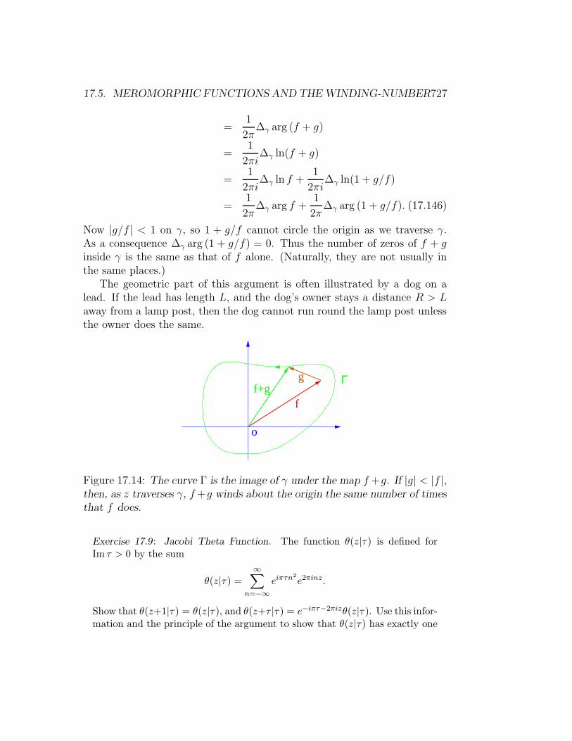
17.5. MEROMORPHIC FUNCTIONS AND THEWINDING-NUMBER727
=1
2π∆γ arg (f + g)
=1
2πi∆γ ln(f + g)
=1
2πi∆γ ln f +
1
2πi∆γ ln(1 + g/f)
=1
2π∆γ arg f +
1
2π∆γ arg (1 + g/f). (17.146)
Now |g/f | < 1 on γ, so 1 + g/f cannot circle the origin as we traverse γ.As a consequence ∆γ arg (1 + g/f) = 0. Thus the number of zeros of f + ginside γ is the same as that of f alone. (Naturally, they are not usually inthe same places.)
The geometric part of this argument is often illustrated by a dog on alead. If the lead has length L, and the dog’s owner stays a distance R > Laway from a lamp post, then the dog cannot run round the lamp post unlessthe owner does the same.
gf+g
o
f
Γ
Figure 17.14: The curve Γ is the image of γ under the map f+g. If |g| < |f |,then, as z traverses γ, f+g winds about the origin the same number of timesthat f does.
Exercise 17.9: Jacobi Theta Function. The function θ(z|τ) is defined forIm τ > 0 by the sum
θ(z|τ) =∞∑
n=−∞eiπτn
2
e2πinz.
Show that θ(z+1|τ) = θ(z|τ), and θ(z+τ |τ) = e−iπτ−2πizθ(z|τ). Use this infor-mation and the principle of the argument to show that θ(z|τ) has exactly one

728 CHAPTER 17. COMPLEX ANALYSIS I
zero in each unit cell of the Bravais lattice comprising the points z = m+ nτ ;m,n ∈ Z. Show that these zeros are located at z = (m+ 1/2) + (n+ 1/2)τ .
Exercise 17.10: Use Rouche’s theorem to find the number of roots of theequation z5 + 15z + 1 = 0 lying within the circles, i) |z| = 2, ii) |z| = 3/2.
17.6 Analytic Functions and Topology
17.6.1 The Point at Infinity
Some functions, f(z) = 1/z for example, tend to a fixed limit (here 0) as zbecome large, independently of in which direction we set off towards infinity.Others, such as f(z) = exp z, behave quite differently depending on whatdirection we take as |z| becomes large.
To accommodate the former type of function, and to be able to legiti-mately write f(∞) = 0 for f(z) = 1/z, it is convenient to add “∞” to theset of complex numbers. Technically, we are constructing the one-point com-pactification of the locally compact space C. We often portray this extendedcomplex plane as a sphere S2 (the Riemann sphere), using stereographicprojection to locate infinity at the north pole, and 0 at the south pole.
N
z
P
S
Figure 17.15: Stereographic mapping of the complex plane to the 2-Sphere.
By the phrase a open neighbourhood of z, we mean an open set containingz. We use the stereographic map to define an open neighbourhood of infinityas the stereographic image of a open neighbourhood of the north pole. Withthis definition, the extended complex plane C ∪ ∞ becomes topologicallya sphere, and in particular, becomes a compact set.

17.6. ANALYTIC FUNCTIONS AND TOPOLOGY 729
If we wish to study the behaviour of a function “at infinity,” we use themap z 7→ ζ = 1/z to bring ∞ to the origin, and study the behaviour of thefunction there. Thus the polynomial
f(z) = a0 + a1z + · · ·+ aNzN (17.147)
becomesf(ζ) = a0 + a1ζ
−1 + · · ·+ aNζ−N , (17.148)
and so has a pole of orderN at infinity. Similarly, the function f(z) = z−3 hasa zero of order three at infinity, and sin z has an isolated essential singularitythere.
We must be a careful about defining residues at infinity. The residue ismore a property of the 1-form f(z) dz than of the function f(z) alone, andto find the residue we need to transform the dz as well as f(z). For example,if we set z = 1/ζ in dz/z we have
dz
z= ζ d
(1
ζ
)= −dζ
ζ, (17.149)
so the 1-form (1/z) dz has a pole at z = 0 with residue 1, and has a polewith residue −1 at infinity—even though the function 1/z has no pole there.This 1-form viewpoint is required for compatability with the residue theorem:The integral of 1/z around the positively oriented unit circle is simultane-ously minus the integral of 1/z about the oppositely oriented unit circle, nowregarded as a a positively oriented circle enclosing the point at infinity. Thusif f(z) has of pole of order N at infinity, and
f(z) = · · ·+ a−2z−2 + a−1z
−1 + a0 + a1z + a2z2 + · · ·+ ANz
N
= · · ·+ a−2ζ2 + a−1ζ + a0 + a1ζ
−1 + a2ζ−2 + · · ·+ ANζ
−N
(17.150)
near infinity, then the residue at infinity must be defined to be −a−1, andnot a1 as one might naıvely have thought.
Once we have allowed ∞ as a point in the set we map from, it is onlynatural to add it to the set we map to — in other words to allow ∞ as apossible value for f(z). We will set f(a) =∞, if |f(z)| becomes unboundedlylarge as z → a in any manner. Thus, if f(z) = 1/z we have f(0) =∞.
The map
w =
(z − z0z − z∞
)(z1 − z∞z1 − z0
)(17.151)

730 CHAPTER 17. COMPLEX ANALYSIS I
takes
z0 → 0,
z1 → 1,
z∞ → ∞, (17.152)
for example. Using this language, the Mobius maps
w =az + b
cz + d(17.153)
become one-to-one maps of S2 → S2. They are the only such globally con-formal one-to-one maps. When the matrix
(a bc d
)(17.154)
is an element of SU(2), the resulting one–to-one map is a rigid rotation ofthe Riemann sphere. Stereographic projection is thus revealed to be thegeometric origin of the spinor representations of the rotation group.
If an analytic function f(z) has no essential singularities anywhere onthe Riemann sphere then f is rational , meaning that it can be written asf(z) = P (z)/Q(z) for some polynomials P , Q.
We begin the proof of this fact by observing that f(z) can have only afinite number of poles. If, to the contrary, f had an infinite number of polesthen the compactness of S2 would ensure that the poles would have a limitpoint somewhere. This would be a non-isolated singularity of f , and hencean essential singularity. Now suppose we have poles at z1, z2, . . ., zN withprincipal parts
mn∑
m=1
bn,m(z − zn)m
.
If one of the zn is ∞, we first use a Mobius map to move it to some finitepoint. Then
F (z) = f(z)−N∑
n=1
mn∑
m=1
bn,m(z − zn)m
(17.155)
is everywhere analytic, and therefore continuous, on S2. But S2 being com-pact and F (z) being continuous implies that F is bounded. Therefore, by

17.6. ANALYTIC FUNCTIONS AND TOPOLOGY 731
Liouville’s theorem, it is a constant. Thus
f(z) =
N∑
n=1
mn∑
m=1
bn,m(z − zn)m
+ C, (17.156)
and this is a rational function. If we made use of a Mobius map to movea pole at infinity, we use the inverse map to restore the original variables.This manoeuvre does not affect the claimed result because Mobius maps takerational functions to rational functions.
The map z 7→ f(z) given by the rational function
f(z) =P (z)
Q(z)=anz
n + an−1zn−1 + · · · a0
bnzn + bn−1zn−1 + · · · b0(17.157)
wraps the Riemann sphere n times around the target S2. In other words, itis a n-to-one map.
17.6.2 Logarithms and Branch Cuts
The function y = ln z is defined to be the solution to z = exp y. Unfortu-nately, since exp 2πi = 1, the solution is not unique: if y is a solution, so isy + 2πi. Another way of looking at this is that if z = ρ exp iθ, with ρ real,then y = ln ρ + iθ, and the angle θ has the same 2πi ambiguity. Now thereis no such thing as a “many valued function.” By definition, a function is amachine into which we plug something and get a unique output. To makeln z into a legitimate function we must select a unique θ = arg z for each z.This can be achieved by cutting the z plane along a curve extending fromthe the branch point at z = 0 all the way to infinity. Exactly where we putthis branch cut is not important; what is important is that it serve as animpenetrable fence preventing us from following the continuous evolution ofthe function along a path that winds around the origin.
Similar branch cuts serve to make fractional powers single valued. Wedefine the power zα for for non-integral α by setting
zα = exp α ln z = |z|αeiαθ, (17.158)
where z = |z|eiθ. For the square root z1/2 we get
z1/2 =√|z|eiθ/2, (17.159)

732 CHAPTER 17. COMPLEX ANALYSIS I
where√|z| represents the positive square root of |z|. We can therefore make
this single-valued by a cut from 0 to ∞. To make√
(z − a)(z − b) singlevalued we only need to cut from a to b. (Why? — think this through!).
We can get away without cuts if we imagine the functions being maps fromsome set other than the complex plane. The new set is called a Riemannsurface. It consists of a number of copies of the complex plane, one for eachpossible value of our “multivalued function.” The map from this new surfaceis then single-valued, because each possible value of the function is the valueof the function evaluated at a point on a different copy. The copies of thecomplex plane are called sheets , and are connected to each other in a mannerdictated by the function. The cut plane may now be thought of as a drawingof one level of the multilayered Riemann surface. Think of an architect’s floorplan of a spiral-floored multi-story car park: If the architect starts drawingat one parking spot and works her way round the central core, at some pointshe will find that the floor has become the ceiling of the part already drawn.The rest of the structure will therefore have to be plotted on the plan of thenext floor up — but exactly where she draws the division between one floorand the one above is rather arbitrary. The spiral car-park is a good modelfor the Riemann surface of the ln z function. See figure 17.16.
O
Figure 17.16: Part of the Riemann surface for ln z. Each time we circle theorigin, we go up one level.
To see what happens for a square root, follow z1/2 along a curve circling thebranch point singularity at z = 0. We come back to our starting point withthe function having changed sign; A second trip along the same path wouldbring us back to the original value. The square root thus has only two sheets,and they are cross-connected as shown in figure 17.17.

17.6. ANALYTIC FUNCTIONS AND TOPOLOGY 733
O
Figure 17.17: Part of the Riemann surface for√z. Two copies of C are cross-
connected. Circling the origin once takes you to the lower level. A secondcircuit brings you back to the upper level.
In figures 17.16 and 17.17, we have shown the cross-connections beingmade rather abruptly along the cuts. This is not necessary —there is nosingularity in the function at the cut — but it is often a convenient wayto think about the structure of the surface. For example, the surface for√
(z − a)(z − b) also consists of two sheets. If we include the point at infinity,this surface can be thought of as two spheres, one inside the other, and crossconnected along the cut from a to b.
17.6.3 Topology of Riemann surfaces
Riemann surfaces often have interesting topology. Indeed much of modernalgebraic topology emerged from the need to develop tools to understandmultiply-connected Riemann surfaces. As we have seen, the complex num-bers, with the point at infinity included, have the topology of a sphere. The√
(z − a)(z − b) surface is still topologically a sphere. To see this imaginecontinuously deforming the Riemann sphere by pinching it at the equatordown to a narrow waist. Now squeeze the front and back of the waist to-gether and (imagining that the the surface can pass freely through itself) foldthe upper half of the sphere inside the lower. The result is the precisely thetwo-sheeted
√(z − a)(z − b) surface described above. The Riemann surface
of the function√(z − a)(z − b)(z − c)(z − d), which can be thought of a two
spheres, one inside the other and connected along two cuts, one from a tob and one from c to d, is, however, a torus . Think of the torus as a bicycleinner tube. Imagine using the fingers of your left hand to pinch the front andback of the tube together and the fingers of your right hand to do the sameon the diametrically opposite part of the tube. Now fold the tube about thepinch lines through itself so that one half of the tube is inside the other,and connected to the outer half through two square-root cross-connects. If

734 CHAPTER 17. COMPLEX ANALYSIS I
α
b ca d
β
Figure 17.18: The 1-cycles α and β on the plane with two square-root branchcuts. The dashed part of α lies hidden on the second sheet of the Riemannsurface.
α
β
Figure 17.19: The 1-cycles α and β on the torus.
you have difficulty visualizing this process, figures 17.18 and 17.19 show howthe two 1-cycles, α and β, that generate the homology group H1(T
2) appearwhen drawn on the plane cut from a to b and c to d, and then when drawnon the torus. Observe, in figure 17.18, how the curves in the two-sheetedplane manage to intersect in only one point, just as they do when drawn onthe torus in figure 17.19.
That the topology of the twice-cut plane is that of a torus has importantconsequences. This is because the elliptic integral
w = I−1(z) =
∫ z
z0
dt√(t− a)(t− b)(t− c)(t− d)
(17.160)
maps the twice-cut z-plane 1-to-1 onto the torus, the latter being consideredas the complex w-plane with the points w and w+nω1+mω2 identified. Thetwo numbers ω1,2 are given by
ω1 =
∮
α
dt√(t− a)(t− b)(t− c)(t− d)
,
ω2 =
∮
β
dt√(t− a)(t− b)(t− c)(t− d)
, (17.161)

17.6. ANALYTIC FUNCTIONS AND TOPOLOGY 735
and are called the periods of the elliptic function z = I(w). The map w 7→z = I(w) is a genuine function because the original z is uniquely determinedby w. It is doubly periodic because
I(w + nω1 +mω2) = I(w), n,m ∈ Z. (17.162)
The inverse “function” w = I−1(z) is not a genuine function of z, however,because w increases by ω1 or ω2 each time z goes around a curve deformableinto α or β, respectively. The periods are complicated functions of a, b, c, d.
If you recall our discussion of de Rham’s theorem from chapter 4, youwill see that the ωi are the results of pairing the closed holomorphic 1-form.
“dw” =dz√
(z − a)(z − b)(z − c)(z − d)∈ H1(T 2) (17.163)
with the two generators of H1(T2). The quotation marks about dw are
there to remind us that dw is not an exact form, i.e. it is not the exteriorderivative of a single-valued function w. This cohomological interpretationof the periods of the elliptic function is the origin of the use of the word“period” in the context of de Rham’s theorem. (See section 19.5 for moreinformation on elliptic functions.)
More general Riemann surfaces are oriented 2-manifolds that can bethought of as the surfaces of doughnuts with g holes. The number g is calledthe genus of the surface. The sphere has g = 0 and the torus has g = 1.The Euler character of the Riemann surface of genus g is χ = 2(1− g). Forexample, figure 17.20 shows a surface of genus three. The surface is in onepiece, so dimH0(M) = 1. The other Betti numbers are dimH1(M) = 6 anddimH2(M) = 1, so
χ =2∑
p=0
(−1)pdimHp(M) = 1− 6 + 1 = −4, (17.164)
in agreement with χ = 2(1− 3) = −4. For complicated functions, the genusmay be infinite.
If we have two complex variables z and w then a polynomial relationP (z, w) = 0 defines a complex algebraic curve. Except for degenerate cases,this one (complex) dimensional curve is simultaneously a two (real) dimen-sional Riemann surface. With
P (z, w) = z3 + 3w2z + w + 3 = 0, (17.165)
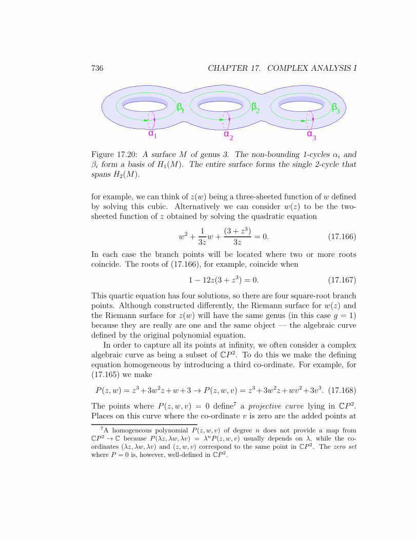
736 CHAPTER 17. COMPLEX ANALYSIS I
1α
β β β
α α
1
2
2
3
3
Figure 17.20: A surface M of genus 3. The non-bounding 1-cycles αi andβi form a basis of H1(M). The entire surface forms the single 2-cycle thatspans H2(M).
for example, we can think of z(w) being a three-sheeted function of w definedby solving this cubic. Alternatively we can consider w(z) to be the two-sheeted function of z obtained by solving the quadratic equation
w2 +1
3zw +
(3 + z3)
3z= 0. (17.166)
In each case the branch points will be located where two or more rootscoincide. The roots of (17.166), for example, coincide when
1− 12z(3 + z3) = 0. (17.167)
This quartic equation has four solutions, so there are four square-root branchpoints. Although constructed differently, the Riemann surface for w(z) andthe Riemann surface for z(w) will have the same genus (in this case g = 1)because they are really are one and the same object — the algebraic curvedefined by the original polynomial equation.
In order to capture all its points at infinity, we often consider a complexalgebraic curve as being a subset of CP 2. To do this we make the definingequation homogeneous by introducing a third co-ordinate. For example, for(17.165) we make
P (z, w) = z3+3w2z+w+3→ P (z, w, v) = z3+3w2z+wv2+3v3. (17.168)
The points where P (z, w, v) = 0 define7 a projective curve lying in CP 2.Places on this curve where the co-ordinate v is zero are the added points at
7A homogeneous polynomial P (z, w, v) of degree n does not provide a map fromCP 2 → C because P (λz, λw, λv) = λnP (z, w, v) usually depends on λ, while the co-ordinates (λz, λw, λv) and (z, w, v) correspond to the same point in CP 2. The zero setwhere P = 0 is, however, well-defined in CP 2.

17.6. ANALYTIC FUNCTIONS AND TOPOLOGY 737
infinity. Places where v is non-zero (and where we may as well set v = 1)constitute the original affine curve.
A generic (non-singular) curve
P (z, w) =∑
r,s
arszrws = 0, (17.169)
with its points at infinity included, has genus
g =1
2(d− 1)(d− 2). (17.170)
Here d = max (r + s) is the degree of the curve. This degree-genus relationis due to Plucker. It is not, however, trivial to prove. Also not easy to proveis Riemann’s theorem of 1852 that any finite genus Riemann surface is thecomplex algebraic curve associated with some two-variable polynomial.
The two assertions in the previous paragraph seem to contradict eachother. “Any” finite genus, must surely include g = 2, but how can a genustwo surface be a complex algebraic curve? There is no integer value of d suchthat (d− 1)(d− 2)/2 = 2. This is where the “non-singular” caveat becomesimportant. An affine curve P (z, w) = 0 is said to be singular at P = (z0, w0)if all of
P (z, w),∂P
∂z,
∂P
∂w,
vanish at P. A projective curve is singular at P ∈ CP 2 if all of
P (z, w, v),∂P
∂z,
∂P
∂w,
∂P
∂v
are zero there. If the curve has a singular point then then it degenerates andceases to be a manifold. Now Riemann’s construction does not guaranteean embedding of the surface into CP 2, only an immersion. The distinctionbetween these two concepts is that an immersed surface is allowed to self-intersect, while an embedded one is not. Being a double root of the definingequation P (z, w) = 0, a point of self-intersection is necessarily a singularpoint.
As an illustration of a singular curve, consider our earlier example of thecurve
w2 = (z − a)(z − b)(z − c)(z − d) (17.171)
whose Riemann surface we know to be a torus once two some points areadded at infinity, and when a, b, c, d are all distinct. The degree-genus formula

738 CHAPTER 17. COMPLEX ANALYSIS I
applied to this degree four curve gives, however, g = 3 instead of the expectedg = 1. This is because the corresponding projective curve
w2v2 = (z − av)(z − bv)(z − cv)(z − dv) (17.172)
has a tacnode singularity at the point (z, w, v) = (0, 1, 0). Rather thaninvestigate this rather complicated singularity at infinity, we will considerthe simpler case of what happens if we allow b to coincide with c. When band c merge, the finite point P = (w0, z0) = (0, b) becomes a singular. Nearthe singularity, the equation defining our curve looks like
0 = w2 − ad (z − b)2, (17.173)
which is the equation of two lines, w =√ad (z − b) and w = −
√ad (z − b),
that intersect at the point (w, z) = (0, b). To understand what is happeningtopologically it is first necessary to realize that a complex line is a copy of Cand hence, after the point at infinity is included, is topologically a sphere. Apair of intersecting complex lines is therefore topologically a pair of spheressharing a common point. Our degenerate curve only looks like a pair oflines near the point of intersection however. To see the larger picture, lookback at the figure of the twice-cut plane where we see that as b approachesc we have an α cycle of zero total length. A zero length cycle means thatthe circumference of the torus becomes zero at P, so that it looks like abent sausage with its two ends sharing the common point P. Instead of twoseparate spheres, our sausage is equivalent to a single two-sphere with twopoints identified.
P
P
P
α
β
α
β
Figure 17.21: A degenerate torus is topologically the same as a sphere withtwo points identified.

17.6. ANALYTIC FUNCTIONS AND TOPOLOGY 739
As it stands, such a set is no longer a manifold because any neighbourhood ofP will contain bits of both ends of the sausage, and therefore cannot be givenco-ordinates that make it look like a region in R2. We can, however, simplyagree to delete the common point, and then plug the resulting holes in thesausage ends with two distinct points. The new set is again a manifold, andtopologically a sphere. From the viewpoint of the pair of intersecting lines,this construction means that we stay on one line, and ignore the other as itpasses through.
A similar resolution of singularities allows us to regard immersed surfacesas non-singular manifolds, and it is this sense that Riemann’s theorem is tobe understood. When n such self-intersection double points are deleted andreplaced by pairs of distinct points The degree-genus formula becomes
g =1
2(d− 1)(d− 2)− n, (17.174)
and this can take any integer value.
17.6.4 Conformal geometry of Riemann surfaces
In this section we recall Hodge’s theory of harmonic forms from section 13.7.1,and see how it looks from a complex-variable perspective. This viewpointreveals a relationship between Riemann surfaces and Riemann manifolds thatforms an important ingredient in string and conformal field theory.
Isothermal co-ordinates and complex structure
Suppose we have a two-dimensional orientable Riemann manifold M withmetric
ds2 = gij dxidxj . (17.175)
In two dimensions gij has three independent components. When we make aco-ordinate transformation we have two arbitrary functions at our disposal,and so we can use this freedom to select local co-ordinates in which only oneindependent component remains. The most useful choice is isothermal (alsocalled conformal) co-ordinates x, y in which the metric tensor is diagonal,gij = eσδij, and so
ds2 = eσ(dx2 + dy2). (17.176)

740 CHAPTER 17. COMPLEX ANALYSIS I
The eσ is called the scale factor or conformal factor . If we set z = x + iyand z = x− iy the metric becomes
ds2 = eσ(z,z)dz dz. (17.177)
We can construct isothermal co-ordinates for some open neighbourhood ofany point inM . If in an overlapping isothermal co-ordinate patch the metricis
ds2 = eτ(ζ,ζ)dζ dζ, (17.178)
and if the co-ordinates have the same orientation, then in the overlap regionζ must be a function only of z and ζ a function only of z. This is so that
eτ(ζ,ζ)dζ dζ = eσ(z,z)∣∣∣∣dz
dζ
∣∣∣∣2
dζ dζ (17.179)
without any dζ2 or dζ2terms appearing. A manifold with an atlas of complex
charts whose change-of-co-ordinate formulae are holomorphic in this way issaid to be a complex manifold , and the co-ordinates endow it with a complexstructure. The existence of a global complex structure allows to us to de-fine the notion of meromorphic and rational functions on M . Our Riemannmanifold is therefore also a Riemann surface.
While any compact, orientable, two-dimensional Riemann manifold hasa complex structure that is determined by the metric, the mapping: metric→ complex structure is not one-to-one. Two metrics gij , gij that are relatedby a conformal scale factor
gij = λ(x1, x2)gij (17.180)
give rise to the same complex structure. Conversely, a pair of two-dimensionalRiemann manifolds having the same complex structure have metrics that arerelated by a scale factor.
The use of isothermal co-ordinates simplifies many computations. Firstly,observe that gij/
√g = δij , the conformal factor having cancelled. If you look
back at its definition, you will see that this means that when the Hodge “⋆”map acts on one-forms, the result is independent of the metric. If ω is aone-form
ω = p dx+ q dy, (17.181)
then⋆ω = −q dx+ p dy. (17.182)

17.6. ANALYTIC FUNCTIONS AND TOPOLOGY 741
Note that, on one-forms,⋆⋆ = −1. (17.183)
With z = x+ iy, z = x− iy, we have
ω =1
2(p− iq) dz + 1
2(p+ iq) dz. (17.184)
Let us focus on the dz part:
A =1
2(p− iq) dz = 1
2(p− iq)(dx+ idy). (17.185)
Then
⋆A =1
2(p− iq)(dy − idx) = −iA. (17.186)
Similarly, with
B =1
2(p+ iq) dz (17.187)
we have⋆B = iB. (17.188)
Thus the dz and dz parts of the original form are separately eigenvectors of ⋆with different eigenvalues. We use this observation to construct a resolutionof the identity Id into the sum of two projection operators
Id =1
2(1 + i⋆) +
1
2(1− i⋆),
= P + P, (17.189)
where P projects on the dz part and P onto the dz part of the form.The original form is harmonic if it is both closed dω = 0, and co-closed
d ⋆ω = 0. Thus, in two dimensions, the notion of being harmonic (i.e. asolution of Laplace’s equation) is independent of what metric we are given.If ω is a harmonic form, then (p− iq)dz and (p+ iq)dz are separately closed.Observe that (p− iq)dz being closed means that ∂z(p− iq) = 0, and so p− iqis a holomorphic (and hence harmonic) function. Since both (p− iq) and dzdepend only on z, we will call (p− iq)dz a holomorphic 1-form. The complexconjugate form
(p− iq)dz = (p + iq)dz (17.190)
then depends only on z and is anti-holomorphic.
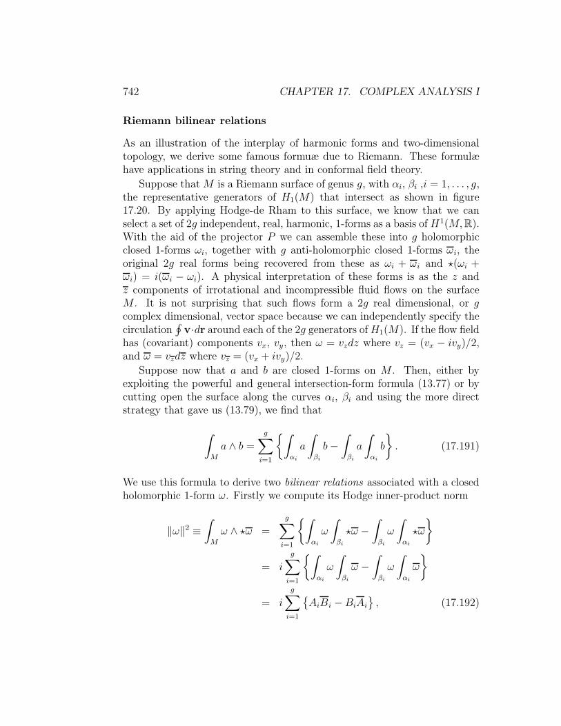
742 CHAPTER 17. COMPLEX ANALYSIS I
Riemann bilinear relations
As an illustration of the interplay of harmonic forms and two-dimensionaltopology, we derive some famous formuæ due to Riemann. These formulæhave applications in string theory and in conformal field theory.
Suppose thatM is a Riemann surface of genus g, with αi, βi ,i = 1, . . . , g,the representative generators of H1(M) that intersect as shown in figure17.20. By applying Hodge-de Rham to this surface, we know that we canselect a set of 2g independent, real, harmonic, 1-forms as a basis ofH1(M,R).With the aid of the projector P we can assemble these into g holomorphicclosed 1-forms ωi, together with g anti-holomorphic closed 1-forms ωi, theoriginal 2g real forms being recovered from these as ωi + ωi and ⋆(ωi +ωi) = i(ωi − ωi). A physical interpretation of these forms is as the z andz components of irrotational and incompressible fluid flows on the surfaceM . It is not surprising that such flows form a 2g real dimensional, or gcomplex dimensional, vector space because we can independently specify thecirculation
∮v·dr around each of the 2g generators ofH1(M). If the flow field
has (covariant) components vx, vy, then ω = vzdz where vz = (vx − ivy)/2,and ω = vzdz where vz = (vx + ivy)/2.
Suppose now that a and b are closed 1-forms on M . Then, either byexploiting the powerful and general intersection-form formula (13.77) or bycutting open the surface along the curves αi, βi and using the more directstrategy that gave us (13.79), we find that
∫
M
a ∧ b =g∑
i=1
∫
αi
a
∫
βi
b−∫
βi
a
∫
αi
b
. (17.191)
We use this formula to derive two bilinear relations associated with a closedholomorphic 1-form ω. Firstly we compute its Hodge inner-product norm
‖ω‖2 ≡∫
M
ω ∧ ⋆ω =
g∑
i=1
∫
αi
ω
∫
βi
⋆ω −∫
βi
ω
∫
αi
⋆ω
= i
g∑
i=1
∫
αi
ω
∫
βi
ω −∫
βi
ω
∫
αi
ω
= i
g∑
i=1
AiBi −BiAi
, (17.192)

17.7. FURTHER EXERCISES AND PROBLEMS 743
where Ai =∫αiω and Bi =
∫βiω. We have used the fact that ω is an anti-
holomorphic 1 form and thus an eigenvector of ⋆ with eigenvalue i. It follows,therefore, that if all the Ai are zero then ‖ω‖ = 0 and so ω = 0.
Let Aij =∫αiωj . The determinant of the matrix Aij is non-zero: If it
were zero, then there would be numbers λi, not all zero, such that
0 = Aijλj =
∫
αi
(ωjλj), (17.193)
but, by (17.192), this implies that ‖ωjλj‖ = 0 and hence ωjλj = 0, contraryto the linear independence of the ωi. We can therefore solve the equations
Aijλjk = δik (17.194)
for the numbers λjk and use these to replace each of the ωi by the linearcombination ωjλji. The new ωi then obey
∫αiωj = δij . From now on we
suppose that this has be done.Define τij =
∫βiωj . Observe that dz ∧ dz = 0 forces ωi ∧ ωj = 0, and
therefore we have a second relation
0 =
∫
M
ωm ∧ ωn =
g∑
i=1
∫
αi
ωm
∫
βi
ωn −∫
βi
ωm
∫
αi
ωn
=
g∑
i=1
δimτin − τimδin
= τmn − τnm. (17.195)
The matrix τij is therefore symmetric. A similar compuation shows that
‖λiωi‖2 = 2λi(Im τij)λj (17.196)
so the matrix (Im τij) is positive definite. The set of such symmetric matriceswhose imaginary part is positive definite is called the Siegel upper half-plane.Not every such matrix correponds to a Riemann surface, but when it does itencodes all information about the shape of the Riemann manifold M that isleft invariant under conformal rescaling.
17.7 Further Exercises and Problems
Exercise 17.11: Harmonic partners. Show that the function
u = sinx cosh y + 2cos x sinh y

744 CHAPTER 17. COMPLEX ANALYSIS I
is harmonic. Determine the corresponding analytic function u+ iv.
Exercise 17.12: Mobius Maps. The Map
z 7→ w =az + b
cz + d
is called a Mobius transformation. These maps are important because they arethe only one-to-one conformal maps of the Riemann sphere onto itself.
a) Show that two successive Mobius transformations
z′ =az + b
cz + d, z′′ =
Az′ +B
Cz′ +D
give rise to another Mobius transformation, and show that the rule forcombining them is equivalent to matrix multiplication.
b) Let z1, z2, z3, z4 be complex numbers. Show that a necessary and suffi-cient condition for the four points to be concyclic is that their cross-ratio
z1, z2, z3, z4 def=
(z1 − z4)(z3 − z2)(z1 − z2)(z3 − z4)
be real (Hint: use a well-known property of opposite angles of a cyclicquadrilateral). Show that Mobius transformations leave the cross-ratioinvariant, and thus take circles into circles.
Exercise 17.13: Hyperbolic geometry . The Riemann metric for the Poincare-disc model of Lobachevski’s hyperbolic plane (See exercises 1.7 and 12.13) canbe taken to be
ds2 =4|dz|2
(1− |z|2)2 , |z|2 < 1.
a) Show that the Mobius transformation
z 7→ w = eiλz − aaz − 1
, |a| < 1, λ ∈ R
provides a 1-1 map of the interior of the unit disc onto itself. Show thatthese maps form a group.
b) Show that the hyperbolic-plane metric is left invariant under the groupof maps in part (a). Deduce that such maps are orientation-preservingisometries of the hyperbolic plane.
c) Use the circle-preserving property of the Mobius maps to deduce thatcircles in hyperbolic geometry are represented in the Poincare disc byEuclidean circles that lie entirely within the disc.
17.7. FURTHER EXERCISES AND PROBLEMS 745
The conformal maps of part (a) are in fact the only orientation preservingisometries of the hyperbolic plane. With the exception of circles centered atz = 0, the center of the hyperbolic circle does not coincide with the centerof its representative Euclidean circle. Euclidean circles that are internallytangent to the boundary of the unit disc have infinite hyperbolic radius andtheir hyperbolic centers lie on the boundary of the unit disc and hence athyperbolic infinity. They are known as horocycles.
Exercise 17.14: Rectangle to Ellipse. Consider the map w 7→ z = sinw. Drawa picture of the image, in the z plane, of the interior of the rectangle withcorners u = ±π/2, v = ±λ. (w = u + iv). Show which points correspond tothe corners of the rectangle, and verify that the vertex angles remain π/2. Atwhat points does the isogonal property fail?
Exercise 17.15: The part of the negative real axis where x < −1 is occupiedby a conductor held at potential −V0. The positive real axis for x > +1is similarly occupied by a conductor held at potential +V0. The conductorsextend to infinity in both directions perpendicular to the x− y plane, and sothe potential V satisfies the two-dimensional Laplace equation.
a) Find the image in the ζ plane of the cut z plane where the cuts run from−1 to −∞ and from +1 to +∞ under the map z 7→ ζ = sin−1 z
b) Use your answer from part a) to solve the electrostatic problem andshow that the field lines and equipotentials are conic sections of the formax2+by2 = 1. Find expressions for a and b for the both the field lines andthe equipotentials and draw a labelled sketch to illustrate your results.
Exercise 17.16: Draw the image under the map z 7→ w = eπz/a of the infinitestrip S, consisting of those points z = x + iy ∈ C for which 0 < y < a.Label enough points to show which point in the w plane corresponds to whichin the z plane. Hence or otherwise show that the Dirichlet Green functionG(x, y;x0, y0) that obeys
∇2G = δ(x− x0)δ(y − y0)
in S, and G(x, y;x0, y0) = 0 for (x, y) on the boundary of S, can be written as
G(x, y;x0, y0) =1
2πln | sinh(π(z − z0)/2a)| + . . .
The dots indicate the presence of a second function, similar to the first, thatyou should find. Assume that (x0, y0) ∈ S.

746 CHAPTER 17. COMPLEX ANALYSIS I
Exercise 17.17: State Laurent’s theorem for functions analytic in an annulus.Include formulae for the coefficients of the expansion. Show that, suitablyinterpreted, this theorem reduces to a form of Fourier’s theorem for functionsanalytic in a neighbourhood of the unit circle.
Exercise 17.18: Laurent Paradox. Show that in the annulus 1 < |z| < 2 thefunction
f(z) =1
(z − 1)(2 − z)has a Laurent expansion in powers of z. Find the coefficients. The part of theseries with negative powers of z does not terminate. Does this mean that f(z)has an essential singularity at z = 0?
Exercise 17.19: Assuming the following series
1
sinh z=
1
z− 1
6z +
7
16z3 + . . . ,
evaluate the integral
I =
∮
|z|=1
1
z2 sinh zdz.
Now evaluate the integral
I =
∮
|z|=4
1
z2 sinh zdz.
(Hint: The zeros of sinh z lie at z = nπi.)
Exercise 17.20: State the theorem relating the difference between the numberof poles and zeros of f(z) in a region to the winding number of argument off(z). Hence, or otherwise, evaluate the integral
I =
∮
C
5z4 + 1
z5 + z + 1dz
where C is the circle |z| = 2. Prove, including a statement of any releventtheorem, any assertions you make about the locations of the zeros of z5+z+1.
Exercise 17.21: Arcsine branch cuts. Let w = sin−1z. Show that
w = nπ ± i lniz +√
1− z2
with the ± being selected depending on whether n is odd or even. Wherewould you put cuts to ensure that w is a single-valued function?

17.7. FURTHER EXERCISES AND PROBLEMS 747
12 3
45
67
8
β1 β2
α2α1
Figure 17.22: Concurrent 1-cycles on a genus-2 surface.
1
6
3
45
2
7
8
α1 L
β1 L
α1 R
β1 R
β2 R
α2 L
β2 L
α 2 R
Figure 17.23: The cut-open genus-2 surface. The superscripts L and R denoterespectively the left and right sides of each 1-cycle, viewed from the directionof the arrow orienting the cycle.

748 CHAPTER 17. COMPLEX ANALYSIS I
Problem 17.22: Cutting open a genus-2 surface. The Riemann surface for thefunction
y =√
(z − a1)(z − a2)(z − a3)(z − a4)(z − a5)(z − a6)
has genus g = 2. Such a surface M is sketched in figure 17.22, where the fourindependent 1-cycles α1,2 and β1,2 that generate H1(M) have been drawn sothat they share a common vertex.
a) Realize the genus-2 surface as two copies of C∪ ∞ cross-connected bythree square-root branch cuts. Sketch how the 1-cycles αi and βi, i = 1, 2of figure 17.22 appear when drawn on your thrice-cut plane.
b) Cut the surface open along the four 1-cycles, and convince yourself thatresulting surface is homeomorphic to the octagonal region appearing infigure 17.23.
c) Apply the direct method that gave us (13.79) to the octagonal region ofpart b). Hence show that for closed 1-forms a, b, on the surface we have
∫
Ma ∧ b =
2∑
i=1
∫
αi
a
∫
βi
b−∫
βi
a
∫
αi
b
.

Chapter 18
Applications of ComplexVariables
In this chapter we will find uses what we have learned of complex variables.The applications will range from the elementary to the sophisticated.
18.1 Contour Integration Technology
The goal of contour integration technology is to evaluate ordinary, real-variable, definite integrals. We have already met the basic tool, the residuetheorem:
Theorem: Let f(z) be analytic within and on the boundary Γ = ∂D of asimply connected domain D, with the exception of finite number of pointsat which the function has poles. Then
∮
Γ
f(z) dz =∑
poles ∈ D2πi (residue at pole).
18.1.1 Tricks of the Trade
The effective application of the residue theorem is something of an art, butthere are useful classes of integrals which we can learn to recognize.
749
750 CHAPTER 18. APPLICATIONS OF COMPLEX VARIABLES
Rational Trigonometric Expressions
Integrals of the form ∫ 2π
0
F (cos θ, sin θ) dθ (18.1)
are dealt with by writing cos θ = 12(z + z), sin θ = 1
2i(z − z) and integrating
around the unit circle. For example, let a, b be real and b < a, then
I =
∫ 2π
0
dθ
a+ b cos θ=
2
i
∮
|z|=1
dz
bz2 + 2az + b=
2
ib
∮dz
(z − α)(z − β) .(18.2)
Since αβ = 1, only one pole is within the contour. This is at
α = (−a +√a2 − b2)/b. (18.3)
The residue is2
ib
1
α− β =1
i
1√a2 − b2
. (18.4)
Therefore, the integral is given by
I =2π√a2 − b2
. (18.5)
These integrals are, of course, also do-able by the “t” substitution t =tan(θ/2), whence
sin θ =2t
1 + t2, cos θ =
1− t21 + t2
, dθ =2dt
1 + t2, (18.6)
followed by a partial fraction decomposition. The labour is perhaps slightlyless using the contour method.
Rational Functions
Integrals of the form ∫ ∞
−∞R(x) dx, (18.7)
where R(x) is a rational function of x with the degree of the denominatorexceeding the degree of the numerator by two or more, may be evaluatedby integrating around a rectangle from −A to +A, A to A + iB, A + iB to
18.1. CONTOUR INTEGRATION TECHNOLOGY 751
−A + iB, and back down to −A. Because the integrand decreases at leastas fast as 1/|z|2 as z becomes large, we see that if we let A,B → ∞, thecontributions from the unwanted parts of the contour become negligeable.Thus
I = 2πi(∑
Residues of poles in upper half-plane). (18.8)
We could also use a rectangle in the lower half-plane with the result
I = −2πi(∑
Residues of poles in lower half-plane), (18.9)
This must give the same answer.
For example, let n be a positive integer and consider
I =
∫ ∞
−∞
dx
(1 + x2)n. (18.10)
The integrand has an n-th order pole at z = ±i. Suppose we close the contourin the upper half-plane. The new contour encloses the pole at z = +i andwe therefore need to compute its residue. We set z − i = ζ and expand
1
(1 + z2)n=
1
[(i+ ζ)2 + 1]n=
1
(2iζ)n
(1− iζ
2
)−n
=1
(2iζ)n
(1 + n
(iζ
2
)+n(n+ 1)
2!
(iζ
2
)2
+ · · ·).(18.11)
The coefficient of ζ−1 is
1
(2i)nn(n + 1) · · · (2n− 2)
(n− 1)!
(i
2
)n−1
=1
22n−1i
(2n− 2)!
((n− 1)!)2. (18.12)
The integral is therefore
I =π
22n−2
(2n− 2)!
((n− 1)!)2. (18.13)
These integrals can also be done by partial fractions.

752 CHAPTER 18. APPLICATIONS OF COMPLEX VARIABLES
18.1.2 Branch-cut integrals
Integrals of the form
I =
∫ ∞
0
xα−1R(x)dx, (18.14)
where R(x) is rational, can be evaluated by integration round a slotted circle(or “key-hole”) contour.
y
x−1
Figure 18.1: A slotted circle contour Γ of outer radius Λ and inner radius ǫ.
A little more work is required to extract the answer, though.
For example, consider
I =
∫ ∞
0
xα−1
1 + xdx, 0 < Reα < 1. (18.15)
The restrictions on the range of α are necessary for the integral to convergeat its upper and lower limits.
We take Γ to be a circle of radius Λ centred at z = 0, with a slot indenta-tion designed to exclude the positive real axis, which we take as the branchcut of zα−1, and a small circle of radius ǫ about the origin. The branch ofthe fractional power is defined by setting
zα−1 = exp[(α− 1)(ln |z|+ iθ)], (18.16)

18.1. CONTOUR INTEGRATION TECHNOLOGY 753
where we will take θ to be zero immediately above the real axis, and 2πimmediately below it. With this definition the residue at the pole at z = −1is eiπ(α−1). The residue theorem therefore tells us that
∮
Γ
zα−1
1 + zdz = 2πieπi(α−1). (18.17)
The integral decomposes as
∮
Γ
zα−1
1 + zdz =
∮
|z|=Λ
zα−1
1 + zdz + (1− e2πi(α−1))
∫ Λ
ǫ
xα−1
1 + xdx−
∮
|z|=ǫ
zα−1
1 + zdz.
(18.18)As we send Λ off to infinity we can ignore the “1” in the denominator com-pared to the z, and so estimate
∣∣∣∣∮
|z|=Λ
zα−1
1 + zdz
∣∣∣∣→∣∣∣∣∮
|z|=Λ
zα−2dz
∣∣∣∣ ≤ 2πΛ× ΛRe (α)−2. (18.19)
This tends to zero provided that Reα < 1. Similarly, provided 0 < Reα, theintegral around the small circle about the origin tends to zero with ǫ. Thus
−eπiα2πi =(1− e2πi(α−1)
)I. (18.20)
We conclude that
I =2πi
(eπiα − e−πiα) =π
sin πα. (18.21)
Exercise 18.1: Using the slotted circle contour, show that
I =
∫ ∞
0
xp−1
1 + x2dx =
π
2 sin(πp/2)=π
2cosec (πp/2), 0 < p < 2.
Exercise 18.2: Integrate za−1/(z − 1) around a contour Γ1 consisting of asemicircle in the upper half plane together with the real axis indented atz = 0 and z = 1

754 CHAPTER 18. APPLICATIONS OF COMPLEX VARIABLES
x
y
1
Figure 18.2: The contour Γ1.
to get
0 =
∮
Γ
za−1
z − 1dz = P
∫ ∞
0
xa−1
x− 1dx− iπ + (cos πa+ i sinπa)
∫ ∞
0
xa−1
x+ 1dx.
As usual, the symbol P in front of the integral sign denotes a principal partintegral, meaning that we must omit an infinitesimal segment of the contoursymmetrically disposed about the pole at z = 1. The term −iπ comes fromintegrating around the small semicircle about this point. We get −1/2 of theresidue because we have only a half circle, and that traversed in the “wrong”direction. Warning: this fractional residue result is only true when we indentto avoid a simple pole—i.e. one that is of order one.
Now take real and imaginary parts and deduce that
∫ ∞
0
xa−1
1 + xdx =
π
sinπα, 0 < Re a < 1,
and
P
∫ ∞
0
xa−1
1− xdx = π cot πa, 0 < Re a < 1.
18.1.3 Jordan’s Lemma
We often need to evaluate Fourier integrals
I(k) =
∫ ∞
−∞eikxR(x) dx (18.22)

18.1. CONTOUR INTEGRATION TECHNOLOGY 755
with R(x) a rational function. For example, the Green function for theoperator −∂2x +m2 is given by
G(x) =
∫ ∞
−∞
dk
2π
eikx
k2 +m2. (18.23)
Suppose x ∈ R and x > 0. Then, in contrast to the analogous integralwithout the exponential function, we have no flexibility in closing the contourin the upper or lower half-plane. The function eikx grows without limit aswe head south in the lower half-plane, but decays rapidly in the upper half-plane. This means that we may close the contour without changing the valueof the integral by adding a large upper-half-plane semicircle.
R
k
im
−im
Figure 18.3: Closing the contour in the upper half-plane.
The modified contour encloses a pole at k = im, and this has residuei/(2m)e−mx. Thus
G(x) =1
2me−mx, x > 0. (18.24)
For x < 0, the situation is reversed, and we must close in the lower half-plane.The residue of the pole at k = −im is −i/(2m)emx, but the minus sign iscancelled because the contour goes the “wrong way” (clockwise). Thus
G(x) =1
2me+mx, x < 0. (18.25)
We can combine the two results as
G(x) =1
2me−m|x|. (18.26)

756 CHAPTER 18. APPLICATIONS OF COMPLEX VARIABLES
The formal proof that the added semicircles make no contribution to theintegral when their radius becomes large is known as Jordan’s Lemma:Lemma: Let Γ be a semicircle, centred at the origin, and of radius R. Sup-pose
i) that f(z) is meromorphic in the upper half-plane;ii) that f(z) tends uniformly to zero as |z| → ∞ for 0 < arg z < π;iii) the number λ is real and positive.
Then ∫
Γ
eiλzf(z) dz → 0, as R→∞. (18.27)
To establish this, we assume that R is large enough that |f | < ǫ on thecontour, and make a simple estimate
∣∣∣∣∫
Γ
eiλzf(z) dz
∣∣∣∣ < 2Rǫ
∫ π/2
0
e−λR sin θ dθ
< 2Rǫ
∫ π/2
0
e−2λRθ/π dθ
=πǫ
λ(1− e−λR) < πǫ
λ. (18.28)
In the second inequality we have used the fact that (sin θ)/θ ≥ 2/π for anglesin the range 0 < θ < π/2. Since ǫ can be made as small as we like, the lemmafollows.Example: Evaluate
I(α) =
∫ ∞
−∞
sin(αx)
xdx. (18.29)
We have
I(α) = Im
∫ ∞
−∞
exp iαz
zdz
. (18.30)
If we take α > 0, we can close in the upper half-plane, but our contour mustexclude the pole at z = 0. Therefore
0 =
∫
|z|=R
exp iαz
zdz −
∫
|z|=ǫ
exp iαz
zdz +
∫ −ǫ
−R
exp iαx
xdx+
∫ R
ǫ
exp iαx
xdx.
(18.31)As R → ∞, we can ignore the big semicircle, the rest, after letting ǫ → 0,gives
0 = −iπ + P
∫ ∞
−∞
eiαx
xdx. (18.32)

18.1. CONTOUR INTEGRATION TECHNOLOGY 757
Again, the symbol P denotes a principal part integral. The −iπ comes fromthe small semicircle. We get −1/2 the residue because we have only a halfcircle, and that traversed in the “wrong” direction. (Remember that thisfractional residue result is only true when we indent to avoid a simple pole—i.e one that is of order one.)
Reading off the real and imaginary parts, we conclude that
∫ ∞
−∞
sinαx
xdx = π, P
∫ ∞
−∞
cosαx
xdx = 0, α > 0. (18.33)
No “P” is needed in the sine integral, as the integrand is finite at x = 0.If we relax the condition that α > 0 and take into account that sine is an
odd function of its argument, we have
∫ ∞
−∞
sinαx
xdx = π sgnα. (18.34)
This identity is called Dirichlet’s discontinuous integral .We can interpret Dirichlet’s integral as giving the Fourier transform of
the principal part distribution P (1/x) as
P
∫ ∞
−∞
eiωx
xdx = iπ sgnω. (18.35)
This will be of use later in the chapter.
Example:
x
y
Figure 18.4: Quadrant contour.
758 CHAPTER 18. APPLICATIONS OF COMPLEX VARIABLES
We will evaluate the integral∮
C
eizza−1 dz (18.36)
about the first-quadrant contour shown above. Observe that when 0 < a < 1neither the large nor the small arc makes a contribution, and that there areno poles. Hence, we deduce that
0 =
∫ ∞
0
eixxa−1 dx− i∫ ∞
0
e−yya−1e(a−1)π2i dy, 0 < a < 1. (18.37)
Taking real and imaginary parts, we find∫ ∞
0
xa−1 cosx dx = Γ(a) cos(π2a), 0 < a < 1,
∫ ∞
0
xa−1 sin x dx = Γ(a) sin(π2a), 0 < a < 1, (18.38)
where
Γ(a) =
∫ ∞
0
ya−1e−y dy (18.39)
is the Euler Gamma function.Example: Fresnel integrals. Integrals of the form
C(t) =
∫ t
0
cos(πx2/2) dx, (18.40)
S(t) =
∫ t
0
sin(πx2/2) dx, (18.41)
occur in the theory of diffraction and are called Fresnel integrals after Au-gustin Fresnel. They are naturally combined as
C(t) + iS(t) =
∫ t
0
eiπx2/2 dx. (18.42)
The limit as t→∞ exists and is finite. Even though the integrand does nottend to zero at infinity, its rapid oscillation for large x is just sufficient toensure convergence.1
1We can exhibit this convergence by setting x2 = s and then integrating by parts toget
∫ t
0
eiπx2/2 dx =
1
2
∫ 1
0
eiπs/2ds
s1/2+
[eiπs/2
πis1/2
]t2
1
+1
2πi
∫ t2
1
eiπs/2ds
s3/2.
The right hand side is now manifestly convergent as t→∞.

18.1. CONTOUR INTEGRATION TECHNOLOGY 759
As t varies, the complex function C(t)+iS(t) traces out the Cornu Spiral ,named after Marie Alfred Cornu, a 19th century French optical physicist.
-0.75 -0.5 -0.25 0.25 0.5 0.75
-0.6
-0.4
-0.2
0.2
0.4
0.6
Figure 18.5: The Cornu spiral C(t) + iS(t) for t in the range −8 < t < 8.The spiral in the first quadrant corresponds to positive values of t.
We can evaluate the limiting value
C(∞) + iS(∞) =
∫ ∞
0
eiπx2/2 dx (18.43)
by deforming the contour off the real axis and onto a line of length L runninginto the first quadrant at 45, this being the direction of most rapid decreaseof the integrand.
L
y
x
Figure 18.6: Fresnel contour.

760 CHAPTER 18. APPLICATIONS OF COMPLEX VARIABLES
A circular arc returns the contour to the axis whence it continues to ∞, butan estimate similar to that in Jordan’s lemma shows that the arc and thesubsequent segment on the real axis make a negligeable contribution when Lis large. To evaluate the integral on the radial line we set z = eiπ/4s, and so
∫ eiπ/4∞
0
eiπz2/2 dz = eiπ/4
∫ ∞
0
e−πs2/2 ds =
1√2eiπ/4 =
1
2(1 + i). (18.44)
Figure 18.5 shows how C(t) + iS(t) orbits the limiting point 0.5 + 0.5i andslowly spirals in towards it. Taking real and imaginary parts we have
∫ ∞
0
cos
(πx2
2
)dx =
∫ ∞
0
sin
(πx2
2
)dx =
1
2. (18.45)
18.2 The Schwarz Reflection Principle
Theorem (Schwarz): Let f(z) be analytic in a domain D where ∂D includesa segment of the real axis. Assume that f(z) is real when z is real. Thenthere is a unique analytic continuation of f into the region D (the mirrorimage of D in the real axis) given by
g(z) =
f(z), z ∈ D,f(z), z ∈ D,either, z ∈ R.
(18.46)
x
y
D
D
Figure 18.7: The domain D and its mirror image D.

18.2. THE SCHWARZ REFLECTION PRINCIPLE 761
The proof invokes Morera’s theorem to show analyticity, and then appealsto the uniqueness of analytic continuations. Begin by looking at a closedcontour lying only in D: ∮
C
f(z) dz, (18.47)
where C = η(t) is the image of C = η(t) ⊂ D under reflection in thereal axis. We can rewrite this as
∮
C
f(z) dz =
∮f(η)
dη
dtdt =
∮f(η)
dη
dtdt =
∮
C
f(η) dz = 0. (18.48)
At the last step we have used Cauchy and the analyticity of f in D. Morera’stheorem therefore confirms that g(z) is analytic in D. By breaking a generalcontour up into parts in D and parts in D, we can similarly show that g(z)is analytic in D ∪D.
The important corollary is that if f(z) is analytic, and real on somesegment of the real axis, but has a cut along some other part of the real axis,then f(x+ iǫ) = f(x− iǫ) as we go over the cut. The discontinuity disc f istherefore 2Im f(x+ iǫ).
Suppose f(z) is real on the negative real axis, and goes to zero as |z| → ∞,then applying Cauchy to the contour Γ depicted in figure 18.8.
y
x
ζ
Figure 18.8: The contour Γ for the dispersion relation. .

762 CHAPTER 18. APPLICATIONS OF COMPLEX VARIABLES
we find
f(ζ) =1
π
∫ ∞
0
Im f(x+ iǫ)
x− ζ dx, (18.49)
for ζ within the contour. This is an example of a dispersion relation. Thename comes from the prototypical application of this technology to opticaldispersion, i.e. the variation of the refractive index with frequency.
If f(z) does not tend to zero at infinity then we cannot ignore the con-tribution to Cauchy’s formula from the large circle. We can, however, stillwrite
f(ζ) =1
2πi
∮
Γ
f(z)
z − ζ dz, (18.50)
and
f(b) =1
2πi
∮
Γ
f(z)
z − b dz, (18.51)
for some convenient point b within the contour. We then subtract to get
f(ζ) = f(b) +(ζ − b)2πi
∫
Γ
f(z)
(z − b)(z − ζ) dz. (18.52)
Because of the extra power of z downstairs in the integrand, we only need fto be bounded at infinity for the contribution of the large circle to tend tozero. If this is the case, we have
f(ζ) = f(b) +(ζ − b)π
∫ ∞
0
Im f(x+ iǫ)
(x− b)(x− ζ) dx. (18.53)
This is called a once-subtracted dispersion relation.The dispersion relations derived above apply when ζ lies within the con-
tour. In physics applications we often need f(ζ) for ζ real and positive. Whathappens as ζ approaches the axis, and we attempt to divide by zero in suchan integral, is summarized by the Plemelj formulæ: If f(ζ) is defined by
f(ζ) =1
π
∫
Γ
ρ(z)
z − ζ dz, (18.54)
where Γ has a segment lying on the real axis, then, if x lies in this segment,
1
2(f(x+ iǫ)− f(x− iǫ)) = iρ(x)
1
2(f(x+ iǫ) + f(x− iǫ)) =
P
π
∫
Γ
ρ(x′)
x′ − x dx′. (18.55)

18.2. THE SCHWARZ REFLECTION PRINCIPLE 763
As always, the “P” means that we are to delete an infinitesimal segment ofthe contour lying symmetrically about the pole.
+ = 2
− =
Figure 18.9: Origin of the Plemelj formulae.
The Plemelj formulæ hold under relatively mild conditions on the functionρ(x). We won’t try to give a general proof, but in the case that ρ is analyticthe result is easy to understand: we can push the contour out of the wayand let ζ → x on the real axis from either above or below. In that case thedrawing in figure 18.9 shows how the the sum of these two limits gives thethe principal-part integral and how their difference gives an integral round asmall circle, and hence the residue ρ(x).
The Plemelj equations usually appear in physics papers as the “iǫ” cabala
1
x′ − x± iǫ = P
(1
x′ − x
)∓ iπδ(x′ − x). (18.56)
A limit ǫ→ 0 is always to be understood in this formula.
Im fRe f
x’−x
x’−x
Figure 18.10: Sketch of the real and imaginary parts of f(x′) = 1/(x′−x−iǫ).
764 CHAPTER 18. APPLICATIONS OF COMPLEX VARIABLES
We can also appreciate the origin of the iǫ rule by examining the followingidentity:
1
x′ − (x± iǫ) =x− x′
(x′ − x)2 + ǫ2± iǫ
(x′ − x)2 + ǫ2. (18.57)
The first term is a symmetrically cut-off version of 1/(x′ − x) and providesthe principal-part integral. The second term sharpens and tends to the deltafunction ±iπδ(x′ − x) as ǫ→ 0.
Exercise 18.3: The Legendre function of the second kind Qn(z) may be definedfor positive integer n by the integral
Qn(z) =1
2
∫ 1
−1
(1− t2)n2n(z − t)n+1
dt, z /∈ [−1, 1].
Use Rodriguez’ formula to show that for x ∈ [−1, 1] we have
Qn(x+ iǫ)−Qn(x− iǫ) = −iπPn(x),
where Pn(x) is the Legendre Polynomial. Show further that Qn(z) satisfies theconditions for the validity of an unsubtracted dispersion relation, and hencededuce Neumann’s formula:
Qn(z) =1
2
∫ 1
−1
Pn(t)
z − t dt, z /∈ [−1, 1].
18.2.1 Kramers-Kronig Relations
Causality is the usual source of analyticity in physical applications. If G(t)is a response function
φresponse(t) =
∫ ∞
−∞G(t− t′)fcause(t′) dt′ (18.58)
then for no effect to anticipate its cause we must have G(t) = 0 for t < 0.The Fourier transform
G(ω) =
∫ ∞
−∞eiωtG(t) dt, (18.59)
is then automatically analytic everywhere in the upper half plane. Suppose,for example, we look at a forced, damped, harmonic oscillator whose dis-placement x(t) obeys
x+ 2γx+ (Ω2 + γ2)x = F (t), (18.60)
18.2. THE SCHWARZ REFLECTION PRINCIPLE 765
where the friction coefficient γ is positive. As we saw earlier, the solution isof the form
x(t) =
∫ ∞
−∞G(t, t′)F (t′)dt′,
where the Green function G(t, t′) = 0 if t < t′. In this case
G(t, t′) =
Ω−1e−γ(t−t
′) sinΩ(t− t′) t > t′
0, t < t′(18.61)
and so
x(t) =1
Ω
∫ t
−∞e−γ(t−t
′) sinΩ(t− t′)F (t′) dt′. (18.62)
Because the integral extends only from 0 to +∞, the Fourier transform ofG(t, 0),
G(ω) ≡ 1
Ω
∫ ∞
0
eiωte−γt sinΩt dt, (18.63)
is nicely convergent when Imω > 0, as evidenced by
G(ω) = − 1
(ω + iγ)2 − Ω2(18.64)
having no singularities in the upper half-plane.2
Another example of such a causal function is provided by the complex,frequency-dependent, refractive index of a material n(ω). This is defined sothat a travelling wave takes the form
ϕ(x, t) = ein(ω)k·x−iωt. (18.65)
We can decompose n into its real and imaginary parts
n(ω) = nR(ω) + inI(ω)
= nR(ω) +i
2|k|γ(ω) (18.66)
2If a pole in a response function manages to sneak into the upper half plane, thenthe system will be unstable to exponentially growing oscillations. This may happen, forexample, when we design an electronic circuit containing a feedback loop. Such poles, andthe resultant instabilities, can be detected by applying the principle of the argument fromthe last chapter. This method leads to the Nyquist stability criterion.

766 CHAPTER 18. APPLICATIONS OF COMPLEX VARIABLES
where γ is the extinction coefficient, defined so that the intensity falls offas I ∝ exp(−γn · x), where n = k/|k| is the direction of propapagation. Anon-zero γ can arise from either energy absorption or scattering out of theforward direction
Being a causal response, the refractive index extends to a function ana-lytic in the upper half plane and n(ω) for real ω is the boundary value
n(ω)physical = limǫ→0
n(ω + iǫ) (18.67)
of this analytic function. Because a real (E = E∗) incident wave must giverise to a real wave in the material, and because the wave must decay in thedirection in which it is propagating, we have the reality conditions
γ(−ω + iǫ) = −γ(ω + iǫ),
nR(−ω + iǫ) = +nR(ω + iǫ) (18.68)
with γ positive for positive frequency.
Many materials have a frequency range |ω| < |ωmin| where γ = 0, sothe material is transparent. For any such material n(ω) obeys the Schwarzreflection principle and so there is an analytic continuation into the lowerhalf-plane. At frequencies ω where the material is not perfectly transparent,the refractive index has an imaginary part even when ω is real. By Schwarz, nmust be discontinuous across the real axis at these frequencies: n(ω + iǫ) =nR + inI 6= n(ω − iǫ) = nR − inI . These discontinuities of 2inI usuallycorrespond to branch cuts.
No substance is able to respond to infinitely high frequency disturbances,so n → 1 as |ω| → ∞, and we can apply our dispersion relation technologyto the function n−1. We will need the contour shown below, which has cutsfor both positive and negative frequencies.

18.2. THE SCHWARZ REFLECTION PRINCIPLE 767
Im
Re
ω
ωωmin−ωmin
Figure 18.11: Contour for the n− 1 dispersion relation.
By applying the dispersion-relation strategy, we find
n(ω) = 1 +1
π
∫ ωmin
−∞
nI(ω′)
ω′ − ω dω′ +
1
π
∫ ∞
ωmin
nI(ω′)
ω′ − ω dω′ (18.69)
for ω within the contour. Using Plemelj we can now take ω onto the real axisto get
nR(ω) = 1 +P
π
∫ ωmin
−∞
nI(ω′)
ω′ − ω dω′ +
P
π
∫ ∞
ωmin
nI(ω′)
ω′ − ω dω′
= 1 +P
π
∫ ∞
ω2min
nI(ω′)
ω′2 − ω2dω′2,
= 1 +c
πP
∫ ∞
ωmin
γ(ω′)
ω′2 − ω2dω′. (18.70)
In the second line we have used the anti-symmetry of nI(ω) to combine thepositive and negative frequency range integrals. In the last line we have usedthe relation ω/k = c to make connection with the way this equation is writtenin R. G. Newton’s authoritative Scattering Theory of Waves and Particles .This relation, between the real and absorptive parts of the refractive index,is called a Kramers-Kronig dispersion relation, after the original authors.3
3H. A. Kramers, Nature, 117 (1926) 775; R. de L. Kronig, J. Opt. Soc. Am. 12 (1926)547

768 CHAPTER 18. APPLICATIONS OF COMPLEX VARIABLES
If n→ 1 fast enough that ω2(n− 1)→ 0 as |ω| → ∞, we can take the fin the dispersion relation to be ω2(n− 1) and deduce that
nR = 1 +c
πP
∫ ∞
ω2min
(ω′2
ω2
)γ(ω′)
ω′2 − ω2dω′, (18.71)
another popular form of Kramers-Kronig. This second relation implies thefirst, but not vice-versa, because the second demands more restrictive be-havior for n(ω).
Similar equations can be derived for other causal functions. A quantityclosely related to the refractive index is the frequency-dependent dielectric“constant”
ǫ(ω) = ǫ1 + iǫ2. (18.72)
Again ǫ→ 1 as |ω| → ∞, and, proceeding as before, we deduce that
ǫ1(ω) = 1 +P
π
∫ ∞
ω2min
ǫ2(ω′)
ω′2 − ω2dω′2. (18.73)
18.2.2 Hilbert transforms
Suppose that f(x) is the boundary value on the real axis of a function every-where analytic in the upper half-plane, and suppose further that f(z) → 0as |z| → ∞ there. Then we have
f(z) =1
2πi
∫ ∞
−∞
f(x)
x− z dx (18.74)
for z in the upper half-plane. This is because we may close the contour withan upper semicircle without changing the value of the integral. For the samereason the integral must give zero when z is taken in the lower half-plane.Using the Plemelj formulæ we deduce that on the real axis,
f(x) =P
πi
∫ ∞
−∞
f(x′)
x′ − x dx′. (18.75)
We can use this strategy to derive the Kramers-Kronig relations even if nInever vanishes, and so we cannot use the Schwarz reflection principle.
The relation (18.75) suggests the definition of the Hilbert transform, Hψ,of a function ψ(x), as
(Hψ)(x) = P
π
∫ ∞
−∞
ψ(x′)
x− x′ dx′. (18.76)

18.2. THE SCHWARZ REFLECTION PRINCIPLE 769
Note the interchange of x, x′ in the denominator of (18.76) when comparedwith (18.75). This switch is to make the Hilbert transform into a convolutionintegral. Equation (18.75) shows that a function that is the boundary valueof a function analytic and tending to zero at infinity in the upper half-plane isautomatically an eigenvector of H with eigenvalue −i. Similarly a functionthat is the boundary value of a function analytic and tending to zero atinfinity in the lower half-plane will be an eigenvector with eigenvalue +i. (Afunction analytic in the entire complex plane and tending to zero at infinitymust vanish identically by Liouville’s theorem.)
Returning now to our original f , which had eigenvalue −i, and decom-posing it as f(x) = fR(x) + ifI(x) we find that (18.75) becomes
fI(x) = (HfR)(x),fR(x) = −(HfI)(x). (18.77)
Conversely, if we are given a real function u(x) and set v(x) = (Hu)(x),then, under some mild restrictions on u (that it lie in some Lp(R), p > 1, forexample, in which case v(x) is also in Lp(R).) the function
f(z) =1
2πi
∫ ∞
−∞
u(x) + iv(x)
x− z dx (18.78)
will be analytic in the upper half plane, tend to zero at infinity there, andhave u(x) + iv(x) as its boundary value as z approaches the real axis fromabove. The last line of (18.77) therefore shows that we may recover u(x)from v(x) as u(x) = −(Hv)(x). The Hilbert transform H : Lp(R) → Lp(R)is therefore invertible, and its inverse is given by H−1 = −H. (Note thatthe Hilbert transform of a constant is zero, but the Lp(R) condition excludesconstants from the domain of H, and so this fact does not conflict withinvertibility.)
Hilbert transforms are useful in signal processing. Given a real signalXR(t) we can take its Hilbert transform so as to find the correspondingimaginary part, XI(t), which serves to make the sum
Z(t) = XR(t) + iXI(t) = A(t)eiφ(t) (18.79)
analytic in the upper half-plane. This complex function is the analytic sig-nal .4 The real quantity A(t) is then known as the instantaneous amplitude,
4D. Gabor, J. Inst. Elec. Eng. (Part 3), 93 (1946) 429-457.
770 CHAPTER 18. APPLICATIONS OF COMPLEX VARIABLES
or envelope, while φ(t) is the instantaneous phase and
ωIF(t) = φ(t) (18.80)
is called the instantaneous frequency (IF). These quantities are used, forexample, in narrow band FM radio, in NMR, in geophysics, and in imageprocessing.
Exercise 18.4: Let f(ω) =∫∞−∞ eiωtf(t) dt denote the Fourier transform of
f(t). Use the formula (18.35) for the Fourier transform of P (1/t), combinedwith the convolution theorem for Fourier transforms, to show that the Fouriertransform of the Hilbert transform of f(t) is
(Hf)(ω) = i sgn(ω)f(ω).
Deduce that the analytic signal is derived from the original real signal bysuppressing all positive frequency components (those proportional to e−iωt
with ω > 0) and multiplying the remaining negative-frequency amplitudes bytwo.
Exercise 18.5: Suppose that ϕ1(x) and ϕ2(x) are real functions with finiteL2(R) norms.
a) Use the Fourier transform result from the previous exercise to show that
〈ϕ1, ϕ2〉 = 〈Hϕ1,Hϕ2〉.
Thus, H is a unitary transformation from L2(R)→ L2(R).b) Use the fact that H2 = −I to deduce that
〈Hϕ1, ϕ2〉 = −〈ϕ1,Hϕ2〉
and so H† = −H.c) Conclude from part b) that
∫ ∞
−∞ϕ1(x)
(P
∫ ∞
−∞
ϕ2(y)
x− y dy)dx =
∫ ∞
−∞ϕ2(y)
(P
∫ ∞
−∞
ϕ1(x)
x− y dx)dy,
i.e., for L2(R), functions, it is legitimate to interchange the order of “P”integration with ordinary integration.
d) By replacing ϕ1(x) by a constant, and ϕ2(x) by the Hilbert transformof a function f with
∫f dx 6= 0, show that it is not always safe to
interchange the order of “P” integration with ordinary integration

18.2. THE SCHWARZ REFLECTION PRINCIPLE 771
Exercise 18.6: Suppose that are given real functions u1(x) and u2(x) and sub-stitute their Hilbert transforms v1 = Hu1, v2 = Hu2 into (18.78) to constructanalytic functions f1(z) and f2(z) that are analytic in the upper half-planeand tend to zero at infinity there. Then, as we approach the real axis fromabove, the product f1(z)f2(z) = F (z) has boundary value
FR(x+ iǫ) + iFI(x+ iǫ) = (u1u2 − v1v2) + i(u1v2 + u2v1).
By assuming that F (z) satisfies the conditions for (18.77) to be applicable tothis boundary value, deduce that
H ((Hu1)u2) +H((Hu2)u1)− (Hu1)(Hu2) = −u1u2. (⋆)
This result5 sometimes appears in the physics literature6 in the guise of thedistributional identity
P
x− yP
y − z +P
y − zP
z − x +P
z − xP
x− y = −π2δ(x − y)δ(x− z),
where P/(x − y) denotes the principal-part distribution P(1/(x− y)
). This
attractively symmetric form conceals the fact that x is being kept fixed, whiley and z are being integrated over in specific orders. As the next exercise shows,were we to freely re-arrange the integration order we could use the identity
1
x− y1
y − z +1
y − z1
z − x +1
z − x1
x− y = 0 x, y, z distinct
to wrongly conclude that the right-hand side of (⋆) is zero.
Problem 18.7: Show that the identity (⋆) from exercise 18.6 can be written as
∫ ∞
−∞
(∫ ∞
−∞
u1(y)u2(z)
(z − y)(y − x)dz)dy =
∫ ∞
−∞
(∫ ∞
−∞
u1(y)u2(z)
(z − y)(y − x)dy)dz−π2u1(x)u2(x),
principal-part integrals being understood where necessary. This is a specialcase of a more general change-of-integration-order formula
∫ ∞
−∞
(∫ ∞
−∞
f(x, y, z)
(z − y)(y − x)dz)dy =
∫ ∞
−∞
(∫ ∞
−∞
f(x, y, z)
(z − y)(y − x)dy)dz−π2f(x, x, x),
5A sufficient condition for its validity is that u1 ∈ Lp1(R), u2 ∈ Lp2(R), where p1 and p2are greater than unity and 1/p1+1/p2 < 1. See F. G. Tricomi, Quart. J. Math. (Oxford),series 2, 2, (1951) 199.
6For example, in R. Jackiw, A. Strominger, Phys. Lett. 99B (1981) 133.

772 CHAPTER 18. APPLICATIONS OF COMPLEX VARIABLES
which was first obtained by G. H. Hardy in 1908. Hardy’s result is oftenreferred to as the Poincare-Bertrand theorem.
Verify Hardy’s formula for the particular case where x is zero and f(0, y, z)is unity when both y and z lie within the interval [−a, a] but zero elsewhere.You will need to show that
∫ ∞
0ln
(a− xa+ x
)2 dx
x= −π2sgn(a).
(Hint: Observe that the integrand is singular at x = |a|. Explain why it islegitimate to evaluate the improper integral by expanding the logarithms as apower series in x or x−1, and then integrating term-by-term.)
Exercise 18.8: Use the licit interchange of “P” integration with ordinary in-tegration to show that
∫ ∞
−∞ϕ(x)
(P
∫ ∞
−∞
ϕ(y)
x− y dy)2
dx =π2
3
∫ ∞
−∞ϕ3(x) dx.
Exercise 18.9: Let f(z) be analytic within the unit circle, and let u(θ) andv(θ) be the boundary values of its real and imaginary parts, respectively, atz = eiθ. Use Plemelj to show that
u(θ) = − 1
2πP
∫ 2π
0v(θ′) cot
(θ − θ′2
)dθ′ +
1
2π
∫ 2π
0u(θ′) dθ′,
v(θ) =1
2πP
∫ 2π
0u(θ′) cot
(θ − θ′2
)dθ′ +
1
2π
∫ 2π
0v(θ′) dθ′.
18.3 Partial-Fraction and Product Expansions
In this section we will study other useful representations of functions whichdevolve from their analyticity properties.
18.3.1 Mittag-Leffler Partial-Fraction Expansion
Let f(z) be a meromorphic function with poles (perhaps infinitely many)at z = zj , (j = 1, 2, 3, . . .), where |z1| < |z2| < . . .. Let Γn be a contourenclosing the first n poles. Suppose further (for ease of description) that thepoles are simple and have residue rn. Then, for z inside Γn, we have
1
2πi
∮
Γn
f(z′)
z′ − z dz′ = f(z) +
n∑
j=1
rjzj − z
. (18.81)

18.3. PARTIAL-FRACTION AND PRODUCT EXPANSIONS 773
We often want to to apply this formula to trigonometric functions whoseperiodicity means that they do not tend to zero at infinity. We thereforeemploy the same strategy that we used for dispersion relations: we subtractf(0) from f(z) to find
f(z)− f(0) = z
2πi
∮
Γn
f(z′)
z′(z′ − z) dz′ +
n∑
j=1
rj
(1
z − zj+
1
zj
). (18.82)
If we now assume that f(z) is uniformly bounded on the Γn — this meaningthat |f(z)| < A on Γn, with the same constant A working for all n — thenthe integral tends to zero as n becomes large, yielding the partial fraction,or Mittag-Leffler , decomposition
f(z) = f(0) +∞∑
j=1
rj
(1
z − zj+
1
zj
)(18.83)
Example: Consider cosec z. The residues of 1/(sin z) at its poles at z = nπare rn = (−1)n. We can take the Γn to be squares with corners (n+1/2)(±1±i)π. A bit of effort shows that cosec is uniformly bounded on them. To usethe formula as given, we first need subtract the pole at z = 0, then
cosec z − 1
z=
∞∑
n=−∞
′
(−1)n(
1
z − nπ +1
nπ
). (18.84)
The prime on the summation symbol indicates that we are omit the n = 0term. The positive and negative n series converge separately, so we can addthem, and write the more compact expression
cosec z =1
z+ 2z
∞∑
n=1
(−1)n 1
z2 − n2π2. (18.85)
Example: A similar method applied to cot z yields
cot z =1
z+
∞∑
n=−∞
′(1
z − nπ +1
nπ
). (18.86)
We can pair terms together to writen this as
cot z =1
z+
∞∑
n=1
(1
z − nπ +1
z + nπ
),
=1
z+
∞∑
n=1
2z
z2 − n2π2(18.87)

774 CHAPTER 18. APPLICATIONS OF COMPLEX VARIABLES
or
cot z = limN→∞
N∑
n=−N
1
z − nπ . (18.88)
In the last formula it is important that the upper and lower limits of summa-tion be the same. Neither the sum over positive n nor the sum over negativen converges separately. By taking asymmetric upper and lower limits wecould therefore obtain any desired number as the limit of the sum.
Exercise 18.10: Use Mittag-Leffler to show that
cosec2z =∞∑
n=−∞
1
(z + nπ)2.
Now use this infinite series to give a one-line proof of the trigonometric identity
N−1∑
m=0
cosec2(z +
mπ
N
)= N2cosec2(Nz).
(Is there a comparably easy elementary derivation of this finite sum?) Take alimit to conclude that
N−1∑
m=1
cosec2(mπN
)=
1
3(N2 − 1).
Exercise 18.11: From the partial fraction expansion for cot z, deduce that
d
dzln[(sin z)/z] =
d
dz
∞∑
n=1
ln(z2 − n2π2).
Integrate this along a suitable path from z = 0, and so conclude that that
sin z = z∞∏
n=1
(1− z2
n2π2
).
Exercise 18.12: By differentiating the partial fraction expansion for cot z, showthat, for k an integer ≥ 1, and Im z > 0, we have
∞∑
n=−∞
1
(z + n)k+1=
(−2πi)k+1
k!
∞∑
n=1
nke2πinz.
This is called Lipshitz’ formula.

18.3. PARTIAL-FRACTION AND PRODUCT EXPANSIONS 775
Exercise 18.13: The Bernoulli numbers are defined by
x
ex − 1= 1 +B1x+
∞∑
k=1
B2kx2k
(2k)!.
The first few are B1 = −1/2, B2 = 1/6, B4 = −1/30. Except for B1, the Bnare zero for n odd. Show that
x cot x = ix+2ix
e2ix − 1= 1−
∞∑
k=1
(−1)k+1B2k22kx2k
(2k)!.
By expanding 1/(x2−n2π2) as a power series in x and comparing coefficients,deduce that, for positive integer k,
∞∑
n=1
1
n2k= (−1)k+1π2k
22k−1
(2k)!B2k.
Exercise 18.14: Euler-Maclaurin sum formula. let f(x) be a real-analyticfunction. Use the formal expansion
D
eD − 1=∑
k
BkDk
k!= 1− 1
2D +
1
6
D2
2!− 1
30
D4
4!+ · · · ,
with D interpreted as d/dx, to obtain
(−f ′(x)−f ′(x+1)−f ′(x+2)+ · · ·) = f(x)− 1
2f ′(x)+
1
6
f ′′(x)2!− 1
30
f (4)
4!+ · · · .
By integrating this formula from 0 to M , where M is an integer, motivate theEuler-Maclaurin sum formula:
12f(0) + f(1) + · · ·+ f(M − 1) + 1
2f(M)
=
∫ M
0f(x) dx+
∞∑
k=1
B2k
(2k)!(f (2k−1)(M)− f (2k−1)(0)).
The left hand side is the trapezium rule approximation to the integral on theright hand side. This derivation gives no insight into whether the infinite-sumcorrection to the trapezium rule converges (usually it does not), or what theerror will be if we truncate the sum after a finite number of terms. Whenf(x) is a polynomial, however, only a finite number of derivatives f (2k−1) arenon-zero, and the result is exact.

776 CHAPTER 18. APPLICATIONS OF COMPLEX VARIABLES
18.3.2 Infinite Product Expansions
We can play a variant of the Mittag-Leffler game with suitable entire func-tions g(z) and derive for them a representation as an infinite product. Sup-pose that g(z) has simple zeros at zi. Then (ln g)′ = g′(z)/g(z) is meromor-phic with poles at zi, all with unit residues. Assuming that it satisfies theuniform boundedness condition, we now use Mittag-Leffler to write
d
dzln g(z) =
g′(z)
g(z)
∣∣∣∣z=0
+∞∑
j=1
(1
z − zj+
1
zj
). (18.89)
Integrating up we have
ln g(z) = ln g(0) + cz +∞∑
j=1
(ln(1− z/zj) +
z
zj
), (18.90)
where c = g′(0)/g(0). We now re-exponentiate to get
g(z) = g(0)ecz∞∏
j=1
(1− z
zj
)ez/zj . (18.91)
Example: Let g(z) = sin z/z, then g(0) = 1, while the constant c, which isthe logarithmic derivative of g at z = 0, is zero, and
sin z
z=
∞∏
n=1
(1− z
nπ
)ez/nπ
(1 +
z
nπ
)e−z/nπ. (18.92)
Thus
sin z = z∞∏
n=1
(1− z2
n2π2
). (18.93)
Convergence of Infinite Products
We have derived several infinite problem formulæ without discussing the issueof their convergence. For products of terms of the form (1+an) with positivean we can reduce the question of convergence to that of
∑∞n=1 an.
To see why this is so, let
pN =
N∏
n=1
(1 + an), an > 0. (18.94)
18.3. PARTIAL-FRACTION AND PRODUCT EXPANSIONS 777
Then we have the inequalities
1 +
N∑
n=1
an < pN < exp
N∑
n=1
an
. (18.95)
The infinite sum and product therefore converge or diverge together. If
P =∞∏
n=1
(1 + |an|), (18.96)
converges, we say that
p =∞∏
n=1
(1 + an), (18.97)
converges absolutely. As with infinite sums, absolute convergence impliesconvergence, but not vice-versa. Unlike infinite sums, however, an infiniteproduct containing negative an can diverge to zero. If (1 + an) > 0 then∏(1 + an) converges if
∑ln(1 + an) does, and we will say that
∏(1 + an)
diverges to zero if∑
ln(1 + an) diverges to −∞.
Exercise 18.15: Show that
N∏
n=1
(1 +
1
n
)= N + 1,
N∏
n=2
(1− 1
n
)=
1
N.
From these deduce that ∞∏
n=2
(1− 1
n2
)=
1
2.
Exercise 18.16: For |z| < 1, show that
∞∏
n=0
(1 + z2
n)=
1
1− z .
(Hint: think binary)
Exercise 18.17: For |z| < 1, show that
∞∏
n=1
(1 + zn) =∞∏
n=1
1
1− z2n−1.
(Hint: 1− x2n = (1− xn)(1 + xn).)

778 CHAPTER 18. APPLICATIONS OF COMPLEX VARIABLES
18.4 Wiener-Hopf Equations II
The theory of Hilbert transforms has shown us some the consequences offunctions being analytic in the upper or lower half-plane. Another applica-tion of these ideas is to Wiener-Hopf equations . Although we have discussedWiener-Hopf integral equations in chapter 9, it is only now that we pos-sess the tools to appreciate the general theory. We begin, however, withthe slightly simpler Wiener-Hopf sum equations, which are their discreteanalogue. Here, analyticity in the upper or lower half-plane is replaced byanalyticity within or without the unit circle.
18.4.1 Wiener-Hopf Sum Equations
Consider the infinite system of equations
yn =
∞∑
m=−∞an−mxm, −∞ < n <∞ (18.98)
where we are given the yn and are seeking the xn.If the an, yn are the Fourier coefficients of smooth complex-valued func-
tions
A(θ) =
∞∑
n=−∞ane
inθ,
Y (θ) =
∞∑
n=−∞yne
inθ, (18.99)
then the systems of equations is, in principle at least, easy to solve. Weintroduce the function
X(θ) =∞∑
n=−∞xne
inθ, (18.100)
and (18.98) becomes
Y (θ) = A(θ)X(θ). (18.101)
From this, the desired xn may be read off as the Fourier expansion coefficientsof Y (θ)/A(θ). We see that A(θ) must be nowhere zero or else the operator Arepresented by the infinite matrix an−m will not be invertible. This technique
18.4. WIENER-HOPF EQUATIONS II 779
is a discrete version of the Fourier transform method for solving the integralequation
y(s) =
∫ ∞
−∞A(s− t)x(t) dt, −∞ < s <∞. (18.102)
The connection with complex analysis is made by regarding A(θ), X(θ), Y (θ)as being functions on the unit circle in the z plane. If they are smooth enoughwe can extend their definition to an annulus about the unit circle, so that
A(z) =
∞∑
n=−∞anz
n,
X(z) =∞∑
n=−∞xnz
n,
Y (z) =∞∑
n=−∞ynz
n. (18.103)
The xn may now be read off as the Laurent expansion coefficients of Y (z)/A(z).The discrete analogue of the Wiener-Hopf integral equation
y(s) =
∫ ∞
0
A(s− t)x(t) dt, 0 ≤ s <∞ (18.104)
is the Wiener-Hopf sum equation
yn =∞∑
m=0
an−mxm, 0 ≤ n <∞. (18.105)
This requires a more sophisticated approach. If you look back at our earlierdiscussion of Wiener-Hopf integral equations in chapter 9, you will see thatthe trick for solving them is to extend the definition y(s) to negative s (anal-ogously, the yn to negative n) and find these values at the same time as wefind x(s) for positive s (analogously, the xn for positive n.)
We proceed by introducing the same functions A(z), X(z), Y (z) as before,but now keep careful track of whether their power-series expansions containpositive or negative powers of z. In doing so, we will discover that theFredholm alternative governing the existence and uniqueness of the solutionswill depend on the winding number N = n(Γ, 0) where Γ is the image of the

780 CHAPTER 18. APPLICATIONS OF COMPLEX VARIABLES
unit circle under the map z 7→ A(z) — in other words, on how many timesA(z) wraps around the origin as z goes once round the unit circle.
Suppose that A(z) is smooth enough that it is analytic in an annulusincluding the unit circle, and that we can factorize A(z) so that
A(z) = λq+(z)zN [q−(z)]
−1, (18.106)
where
q+(z) = 1 +
∞∑
n=1
q+n zn,
q−(z) = 1 +
∞∑
n=1
q−−nz−n. (18.107)
Here we demand that q+(z) be analytic and non-zero for |z| < 1 + ǫ, andthat q−(z) be analytic and non-zero for |1/z| < 1 + ǫ. These no pole, nozero, conditions ensure, via the principle of the argument, that the windingnumbers of q±(z) about the origin are zero, and so all the winding of A(z) isaccounted for by the N -fold winding of the zN factor. The non-zero conditionalso ensures that the reciprocals [q±(z)]
−1 have same class of expansions (i.e.in positive or negative powers of z only) as the direct functions.
We now introduce the notation [F (z)]+ and [F (z)]−, meaning that weexpand F (z) as a Laurent series and retain only the positive powers of z(including z0), or only the negative powers (starting from z−1), respectively.Thus F (z) = [F (z)]++[F (z)]−. We will write Y±(z) = [Y (z)]±, and similarlyfor X(z). We can therefore rewrite (18.105) in the form
λzNq+(z)X+ = [Y+(z) + Y−(z)]q−(z). (18.108)
If N ≥ 0, and we break this equation into its positive and negative powers,we find
[Y+q−]+ = λzNq+(z)X+,
[Y+q−]− = −Y−q−(z). (18.109)
From the first of these equations we can read off the desired xn as the positive-power Laurent coefficients of
X+(z) = [Y+q−]+(λzNq+(z))
−1. (18.110)

18.4. WIENER-HOPF EQUATIONS II 781
As a byproduct, the second alows us to find the coefficient y−n of Y−(z).Observe that there is a condition on Y+ for this to work: the power seriesexpansion of λzNq+(z)X+ starts with zN , and so for a solution to exist thefirst N terms of (Y+q−)+ as a power series in z must be zero. The givenvector yn must therefore satisfy N consistency conditions. A formal way ofexpressing this constraint begins by observing that it means that the range ofthe operator A represented by the matrix an−m falls short, by N dimensions,of the being the entire space of possible yn. This is exactly the situation thatthe notion of a “cokernel” is intended to capture. Recall that if A : V → V ,then CokerA = V/ImA. We therefore have
dim [CokerA] = N.
When N < 0, on the other hand, we have
[Y+(z)q−(z)]+ = [λz−|N |q+(z)X+(z)]+
[Y+(z)q−(z)]− = −Y−(z)q−(z) + [λz−|N |q+(z)X+(z)]−. (18.111)
Here the last term in the second equation contains no more thanN terms. Be-cause of the z−|N |, we can add any to X+ any multiple of Z+(x) = zn[q+(z)]
−1
for n = 0, . . . , N−1, and still have a solution. Thus the solution is not unique.Instead, we have dim [Ker (A)] = |N |.
We have therefore shown that
Index (A)def= dim (KerA)− dim (CokerA) = −N
This connection between a topological quantity – in the present case thewinding number — and the difference in dimension of the kernel and cokernelis an example of an index theorem.
We now need to show that we can indeed factorize A(z) in the desiredmanner. When A(z) is a rational function, the factorization is straightfor-ward: if
A(z) = C
∏n(z − an)∏m(z − bm)
, (18.112)
we simply take
q+(z) =
∏|an|>0(1− z/an)∏|bm|>0(1− z/bm)
, (18.113)

782 CHAPTER 18. APPLICATIONS OF COMPLEX VARIABLES
where the products are over the linear factors corresponding to poles andzeros outside the unit circle, and
q−(z) =
∏|bm|<0(1− bm/z)∏|an|<0(1− an/z)
, (18.114)
containing the linear factors corresponding to poles and zeros inside the unitcircle. The constant λ and the power zN in equation (18.106) are the factorsthat we have extracted from the right-hand sides of (18.113) and (18.114),respectively, in order to leave 1’s as the first term in each linear factor.
More generally, we take the logarithm of
z−NA(z) = λq+(z)(q−(z))−1 (18.115)
to get
ln[z−NA(z)] = ln[λq+(z)]− ln[q−(z)], (18.116)
where we desire ln[λq+(z)] to be the boundary value of a function analyticwithin the unit circle, and ln[q−(z)] the boundary value of function analyticoutside the unit circle and with q−(z) tending to unity as |z| → ∞. Thefactor of z−N in the logarithm serves to undo the winding of the argumentof A(z), and results in a single-valued logarithm on the unit circle. Plemeljnow shows that
Q(z) =1
2πi
∮
|z|=1
ln[ζ−NA(ζ)]
ζ − z dζ (18.117)
provides us with the desired factorization. This function Q(z) is everywhereanalytic except for a branch cut along the unit circle, and its branches, Q+
within and Q− without the circle, differ by ln[z−NA(z)]. We therefore have
λq+(z) = eQ+(z),
q−(z) = eQ−(z). (18.118)
The expression for Q as an integral shows that Q(z) ∼ const./z as |z|goes to infinity and so guarantees that q−(z) has the desired limit of unitythere.
The task of finding this factorization is known as the scalar Riemann-

18.4. WIENER-HOPF EQUATIONS II 783
Hilbert problem. In effect, we are decomposing the infinite matrix
A =
. . ....
......
· · · a0 a1 a2 · · ·· · · a−1 a0 a1 · · ·· · · a−2 a−1 a0 · · ·
......
.... . .
(18.119)
into the product of an upper triangular matrix
U = λ
. . ....
......
· · · 1 q+1 q+2 · · ·· · · 0 1 q+1 · · ·· · · 0 0 1 · · ·
......
.... . .
, (18.120)
a lower triangular matrix L, where
L−1 =
. . ....
......
· · · 1 0 0 · · ·· · · q−−1 1 0 · · ·· · · q−−2 q−−1 1 · · ·
......
.... . .
, (18.121)
has 1’s on the diagonal, and a matrix ΛN which which is zero everywhereexcept for a line of 1’s located N steps above the main diagonal. The setof triangular matrices with unit diagonal form a group, so the inversionrequired to obtain L results in a matrix of the same form. The resultingBirkhoff factorization
A = LΛNU, (18.122)
is an infinite-dimensional extension of the Gauss-Bruhat (or generalized LU)decomposition of a matrix. The finite-dimensional Gauss-Bruhat decompo-sition provides a factorization of a matrix A ∈ GL(n) as
A = LΠU, (18.123)
where L is a lower triangular matrix with 1’s on the diagonal, U is an uppertriangular matrix with no zero’s on the diagonal, and Π is a permutation

784 CHAPTER 18. APPLICATIONS OF COMPLEX VARIABLES
matrix, i.e. a matrix that permutes the basis vectors by having one entry of1 in each row and in each column, and all other entries zero. Our present ΛN
is playing the role of such a matrix. The matrix Π is uniquely determinedby A. The L and U matrices become unique if L is chosen so that ΠTLΠis also lower triangular.
18.4.2 Wiener-Hopf Integral Equations
We now carry over our insights from the simpler sum equations to Weiner-Hopf integral equations
∫ ∞
0
K(x− y)φ(y) dy = f(x), x > 0, (18.124)
by imagining replacing the unit circle by a circle of radius R, and then takingR→∞ in such a way that the sums go over to integrals. In this way manyfeatures are retained: the problem is still solved by factorizing the Fouriertransform
K(k) =
∫ ∞
−∞K(x)eikx dx (18.125)
of the kernel, and there remains an index theorem
dim (KerK)− dim (CokerK) = −N, (18.126)
but N now counts the winding of the phase of K(k) as k ranges over the realaxis:
N =1
2πarg K
∣∣∣k=+∞
k=−∞. (18.127)
One restriction arises though: we will require K to be of the form
K(x− y) = δ(x− y) + g(x− y) (18.128)
for some continuous function g(x). Our discussion is therefore being re-stricted to Wiener-Hopf Integral equations of the second kind.
The restriction comes about about because we will seek to obtain a fac-torization of K as
τ(κ)K(k) = expQ+(k)−Q−(k) = q+(k)(q−(k))−1 (18.129)
18.4. WIENER-HOPF EQUATIONS II 785
where q+(k) ≡ expQ+(k) is analytic and non-zero in the upper half k-planeand q−(k) ≡ expQ−(k) analytic and non-zero in the lower half-plane. Thefactor τ(κ) is a phase such as
τ(k) =
(k + i
k − i
)N, (18.130)
which winds −N times and serves serves to undo the +N phase winding inK. The Q±(k) will be the boundary values from above and below the realaxis, respectively, of
Q(k) =1
2πi
∫ ∞
−∞
ln[τ(κ)K(κ)]
κ− k dκ (18.131)
The convergence of this infinite integral requires that ln[τ(κ)K(k)] go to zeroat infinity, or, in other words,
limk→∞
K(k) = 1. (18.132)
This, in turn, requires that the original K(x) contain a delta function.Example: We will solve the problem
φ(x)− λ∫ ∞
0
e−|x−y|−α(x−y)φ(y) dy = f(x), x > 0. (18.133)
We require that 0 < α < 1. The upper bound on α is necessary for theintegral kernel to be bounded. We will also assume for simplicity that λ <1/2. Following the same strategy as in the sum case, we extend the integralequation to the entire range of x by writing
φ(x)− λ∫ ∞
0
e−|x−y|−α(x−y)φ(y) dy = f(x) + g(x), (18.134)
where f(x) is nonzero only for x > 0 and g(x) is non-zero only for x < 0.The Fourier transform of this equation is
((k + iα)2 + a2
(k + iα)2 + 1
)φ+(k) = f+(k) + g−(k), (18.135)
where a2 = 1− 2λ and the ± subscripts are to remind us that φ(k) and f(k)are analytic in the upper half-plane, and g(k) in the lower. We will use the

786 CHAPTER 18. APPLICATIONS OF COMPLEX VARIABLES
notation H+ for the space of functions analytic in the upper half plane, andH− for functions analytic in the lower half plane, and so
φ+(k), f(+k) ∈ H+, g−(k) ∈ H− (18.136)
We can factorize
K(k) =(k + iα)2 + a2
(k + iα)2 + 1=
[k + i(α− a)][k + i(α− 1)]
[k + i(α + a)]
[k + i(α + 1)](18.137)
Now suppose that a is small enough that α ± a > 0 and so the numeratorhas two zeros in the lower half plane, and the numerator a one zero in eachof the upper and lower half-planes. The change of phase in K(k) as we gofrom minus to plus infinity is therefore −2π, and so the index is N = −1.We should therefore multiply K by
τ(k) =
(k + i
k − i
)−1
(18.138)
before seeking to break it into its q± factors. We can however equally welltake
τ(k) =
(k + i(α− 1)
k + i(α− a)
)(18.139)
as this also undoes the winding and allows us to factorize with
q−(k) = 1, q+(k) =
(k + i(α + a)
k + i(α + 1)
). (18.140)
The resultant equation analagous to (18.108) is therefore
(k + i(α + a)
k + i(α + 1)
)φ+ =
(k + i(α− 1)
k + i(α− a)
)f+ +
(k + i(α− 1)
k + i(α− a)
)g−
q+φ+ = (τq−)f+ + τq−g− (18.141)
The second line of this equation shows the interpretation of the first line interms of the objects in the general theory. The left hand side is in H+ —i.e. analytic in the upper half-plane. The first term on the right is also inH+. (We are lucky. More generally it would have to be decomposed into itsH± parts.) If it were not for the τ(κ), the last term would be in H−, but

18.4. WIENER-HOPF EQUATIONS II 787
it has a potential pole at k = −i(α − a). We therefore remove this pole bysubstracting a term
− β
k + i(α− a)(an element of H+) from each side of the equation before projecting onto theH± parts. After projecting, we find that
H+ :
(k + i(α + a)
k + i(α + 1)
)φ+ −
(k + i(α− 1)
k + i(α− a)
)f+ −
β
k + i(α− a) = 0,
H− :
(k + i(α− 1)
k + i(α− a)
)g− −
β
k + i(α− a) = 0. (18.142)
We solve for φ+(k) and g−(k)
φ+(k) =
((k + iα)2 + 1
(k + iα)2 + a2
)f− − β
(k + i(α + 1)
(k + iα)2 + a2
)
g−(k) =β
k + i(α− 1). (18.143)
Observe g−(k) is always in H− because its only singularity is in the upperhalf-plane for any β. The constant β is therefore arbitrary. Finally, we invertthe Fourier transform, using
F(θ(x)e−αx sinh ax
)= − a
(k + iα)2 + a2, (α± a) > 0, (18.144)
to find that
φ(x) = f(x)− 2λ
a
∫ x
0
e−α(x−y) sinh a(x− y)f(y) dy
+β ′ (a− 1)e−(α+a)x + (a + 1)e−(α−a)x , (18.145)
where β ′ (proportional to β) is an arbitrary constant.By taking α in the range −1 < α < 0 with (α ± a) < 0, we make index
to be N = +1. We will then find there is condition on f(x) for the solutionto exist. This condition is, of course, that f(x) be orthogonal to the solution
φ0(x) =(a− 1)e−(α+a)x + (a + 1)e−(α−a)x (18.146)
of the homogenous adjoint problem, this being the f(x) = 0 case of the α > 0problem that we have just solved.

788 CHAPTER 18. APPLICATIONS OF COMPLEX VARIABLES
18.5 Further Exercises and Problems
Exercise 18.18: Contour Integration: Use the calculus of residues to evaluatethe following integrals:
I1 =
∫ 2π
0
dθ
(a+ b cos θ)2, 0 < b < a.
I2 =
∫ 2π
0
cos2 3θ
1− 2a cos 2θ + a2dθ, 0 < a < 1.
I3 =
∫ ∞
0
xα
(1 + x2)2dx, −1 < α < 2.
These are not meant to be easy! You will have to dig for the residues.
Answers:
I1 =2πa
(a2 − b2)3/2 ,
I2 =π(a3 + 1)
1− a2 =π(1− a+ a2)
1− a ,
I3 =π(1− α)
4 cos(πα/2).
Exercise 18.19: By considering the integral of
f(z) = ln(1− e2iz) = ln(−2ieiz sin z)
around the indented rectangle
iY +iYπ
0 π
Figure 18.12: Indented rectangle.

18.5. FURTHER EXERCISES AND PROBLEMS 789
with vertices 0, π, π+iY , iY , and letting Y become large, evaluate the integral
I =
∫ π
0ln(sinx) dx.
Explain how the fact that ǫ ln ǫ→ 0 as ǫ→ 0 allows us to ignore contributionsfrom the small indentations. You should also provide justification for any otherdiscarded contributions. Take care to make consistent choices of the branch ofthe logarithm, especially if expanding ln(−2ieix sinx) = ix+ ln 2+ ln(sinx)+ln(−i).(Ans: −π ln 2.)
Exercise 18.20: By integrating a suitable function around the quadrant con-taining the point z0 = eiπ/4, evaluate the integral
I(α) =
∫ ∞
0
xα−1
1 + x4dx 0 < α < 4.
It should only be necessary to consider the residue at z0.(Ans: (π/4)cosec (πα/4).)
Exercise 18.21: In section 5.5.1 we considered the causal Green function forthe damped harmonic oscillator
G(t) =
1Ωe
−γt sin(Ωt), t > 0,0, t < 0,
and showed that its Fourier transform∫ ∞
−∞eiωtG(t) dt =
1
Ω2 − (ω + iγ)2, (18.147)
had no singularities in the upper half-plane. Use Jordan’s lemma to computethe inverse Fourier transform
1
2π
∫ ∞
−∞
e−iωt
Ω2 − (ω + iγ)2dω,
and verify that it reproduces G(t).
Problem 18.22: Jordan’s Lemma and one-dimensional scattering theory . Inproblem 4.13 we considered the one-dimensional scattering problem solutions
ψk(x) =
eikx + rL(k)e
−ikx, x ∈ L,tL(k)e
ikx, x ∈ R, k > 0.
=
tR(k)e
ikx, x ∈ L,eikx + rR(k)e
−ikx, x ∈ R. k < 0.
790 CHAPTER 18. APPLICATIONS OF COMPLEX VARIABLES
and claimed that the bound-state contributions to the completeness relationwere given in terms of the reflection and transmission coefficients as
∑
bound
ψ∗n(x)ψn(x
′) = −∫ ∞
−∞
dk
2πrL(k)e
−ik(x+x′), x, x′ ∈ L,
= −∫ ∞
−∞
dk
2πtL(k)e
−ik(x−x′), x ∈ L, x′ ∈ R,
= −∫ ∞
−∞
dk
2πtR(k)e
−ik(x−x′), x ∈ R, x′ ∈ L,
= −∫ ∞
−∞
dk
2πrR(k)e
−ik(x+x′), x, x′ ∈ R.
The eigenfunctions
ψ(+)k (x) =
eikx + rL(k)e
−ikx, x ∈ L,tL(k)e
ikx, x ∈ R,and
ψ(−)k (x) =
tR(k)e
ikx, x ∈ L,eikx + rR(k)e
−ikx, x ∈ R.are initially refined for k real and positive (ψ
(+)k ) or for k real and negative
(ψ(−)k ), but they separately have analytic continuations to all of k ∈ C. The
reflection and transmission coefficients rL,R(k) and tL,R(k) are also analyticfunctions of k, and obey rL,R(k) = r∗L,R(−k∗), tL,R(k) = t∗L,R(−k∗).
a) By inspecting the formulæ for ψ(+)k (x), show that the bound states ψn(x),
with En = −κ2n, are proportional to ψ(+)k (x) evaluated at points k = iκn
on the positive imaginary axis at which rL(k) and tL(k) simultaneouslyhave poles. Similarly show that these same bound states are proportional
to ψ(−)k (x) evaluated at points −iκn on the negative imaginary axis at
which rR(k) and tR(k) have poles. (All these functions ψ(±)k (x), rR,L(k),
tR,L(k), may have branch points and other singularities in the half-planeon the opposite side of the real axis from the bound-state poles.)
b) Use Jordan’s lemma to evaluate the Fourier transforms given above interms of the position and residues of the bound-state poles. Confirmthat your answers are of the form
∑
n
A∗n[sgn(x)]e
−κn|x|An[sgn(x′)]e−κn|x
′|,
as you would expect for the bound-state contribution to the completenessrelation.

18.5. FURTHER EXERCISES AND PROBLEMS 791
Exercise 18.23: Lattice Matsubara sums: Let ωn = expiπ(2n + 1)/N, forn = 0, . . . , N − 1, be the N -th roots of (−1). Show that, for suitable analyticfunctions f(z), the sum
S =1
N
N−1∑
n=0
f(ωn)
can be written as an integral
S =1
2πi
∫
C
dz
z
zN
zN + 1f(z).
Here C consists of a pair of oppositely oriented concentric circles. The annulusformed by the circles should include all the roots of (-1), but exclude allsingularites of f . Use this result to show that, for N even,
1
N
N−1∑
n=0
sinhE
sinh2E + sin2 (2n+1)πN
=1
coshEtanh
NE
2.
Let N → ∞ while scaling E → 0 in some suitable manner, and hence showthat ∞∑
n=−∞
a
a2 + [(2n + 1)π]2=
1
2tanh
a
2.
(Hint: If you are careless, you will end up differing by a factor of two from thislast formula. There are two regions in the finite sum that tend to the infinitesum in the large N limit.)
Problem 18.24: If we define χ(h) = eαxφ(x), and F (x) = eαxf(x), then theWiener-Hopf equation
φ(x)− λ∫ ∞
0e−|x−y|−α(x−y)φ(y) dy = f(x), x > 0.
becomes
χ(x)− λ∫ ∞
0e−|x−y|χ(y) dy = F (x), x > 0,
all mention of α having disappeared! Why then does our answer, worked outin such detail, in section 18.4.2 depend on the parameter α? Show that if αsmall enough that α + a is positive and α − a is negative, then φ(x) really isindependent of α. (Hint: What tacit assumptions about function spaces doesour use of Fourier transforms entail? How does the inverse Fourier transformof [(k + iα)2 + a2]−1 vary with α?)

792 CHAPTER 18. APPLICATIONS OF COMPLEX VARIABLES

Chapter 19
Special Functions and ComplexVariables
In this chapter we will apply complex analytic methods so as to obtain awider view of some of the special functions of mathematical physics than canbe obtained from the real axis. The standard text in this field remains thevenerable Course of Modern Analysis of E. T. Whittaker and G. N. Watson.
19.1 The Gamma Function
We begin by examining how Euler’s “Gamma function” Γ(z) behaves whenz is allowed to become complex. You probably have some acquaintance withthis creature. The usual definition is
Γ(z) =
∫ ∞
0
tz−1e−t dt, Re z > 0, (definition A). (19.1)
The restriction on the real part of z is necessary to make the integral converge.We can, however, analytically continue Γ(z) to a meromorphic function onall of C. An integration by parts, based on
d
dt
(tze−t
)= ztz−1e−t − tze−t, (19.2)
shows that [tze−t
]∞0
= z
∫ ∞
0
tz−1e−t dt−∫ ∞
0
tze−t dt. (19.3)
793

794CHAPTER 19. SPECIAL FUNCTIONS AND COMPLEX VARIABLES
The integrated out part vanishes at both limits, provided the real part of zis greater than zero. Thus we obtain the recurrence relation
Γ(z + 1) = zΓ(z). (19.4)
Since Γ(1) = 1, we deduce that
Γ(n) = (n− 1)!, n = 1, 2, 3, . . . . (19.5)
We can use the recurrence relation (19.4) to extend the definition of Γ(z) tothe left half-plane, where the real part of z is negative. Choosing an integern such that the real part of z + n is positive, we write
Γ(z) =Γ(z + n)
z(z + 1) · · · (z + n− 1). (19.6)
We see that the extended Γ(z) has poles at zero, and at the negative integers.The residue of the pole at z = −n is (−1)n/n!.
We can also view the analytic continuation as an example of Taylor seriessubtraction. Let us recall how this works. Suppose that −1 < Re x < 0.Then, from
d
dt(txe−t) = xtx−1e−t − txe−t (19.7)
we have [txe−t
]∞ǫ
= x
∫ ∞
ǫ
dt tx−1e−t −∫ ∞
ǫ
dt txe−t. (19.8)
Here we have cut off the integral at the lower limit so as to avoid the di-vergence near t = 0. Evaluating the left-hand side and dividing by x wefind
−1
xǫx =
∫ ∞
ǫ
dt tx−1e−t − 1
x
∫ ∞
ǫ
dt txe−t. (19.9)
Since, for this range of x,
−1
xǫx =
∫ ∞
ǫ
dt tx−1, (19.10)
we can rewrite (19.9) as
1
x
∫ ∞
ǫ
dt txe−t =
∫ ∞
ǫ
dt tx−1(e−t − 1
). (19.11)

19.1. THE GAMMA FUNCTION 795
The integral on the right-hand side of this last expression is convergent asǫ→ 0, so we may safely take the limit and find
1
xΓ(x+ 1) =
∫ ∞
0
dt tx−1(e−t − 1
). (19.12)
Since the left-hand side is equal to Γ(x), we have shown that
Γ(x) =
∫ ∞
0
dt tx−1(e−t − 1
), −1 < Rex < 0. (19.13)
Similarly, if −2 < Rex < −1, we can show that
Γ(x) =
∫ ∞
0
dt tx−1(e−t − 1 + t
). (19.14)
Thus the analytic continuation of the original integral is given by a newintegral in which we have subtracted exactly as many terms from the Taylorexpansion of e−t as are needed to just make the integral convergent at thelower limit.
Other useful identities, usually proved by elementary real-variable meth-ods, include Euler’s “Beta function” identity,
B(a, b)def=
Γ(a)Γ(b)
Γ(a + b)=
∫ 1
0
(1− t)a−1tb−1 dt (19.15)
(which, as the Veneziano formula, was the original inspiration for stringtheory) and
Γ(z)Γ(1 − z) = πcosec πz. (19.16)
The proofs of both formulæ begin in the same way: set t = y2, x2, so that
Γ(a)Γ(b) = 4
∫ ∞
0
y2a−1e−y2
dy
∫ ∞
0
x2b−1e−x2
dx
= 4
∫ ∞
0
∫ ∞
0
e−(x2+y2)x2b−1y2a−1 dx dy
= 2
∫ ∞
0
e−r2
(r2)a+b−1 d(r2)
∫ π/2
0
sin2a−1 θ cos2b−1 θ dθ.
We have appealed to Fubini’s theorem twice: once to turn a product ofintegrals into a double integral, and once (after setting x = r cos θ, y =

796CHAPTER 19. SPECIAL FUNCTIONS AND COMPLEX VARIABLES
r sin θ) to turn the double integral back into a product of decoupled integrals.In the second factor of the third line we can now change variables to t = sin2 θand obtain the Beta function identity. If, on the other hand, we put a = 1−z,b = z, we have
Γ(z)Γ(1− z) = 2
∫ ∞
0
e−r2
d(r2)
∫ π/2
0
cot2z−1 θ dθ = 2
∫ π/2
0
cot2z−1 θ dθ.
(19.17)Now set cot θ = ζ . The last integral then becomes (see exercise 18.1):
2
∫ ∞
0
ζ2z−1
ζ2 + 1dζ = π cosec πz, 0 < z < 1, (19.18)
establishing the claimed result. Although this last integral has a restrictionon the range of z (19.16) it holds for all z by analytic continuation. If weput z = 1/2, we find that (Γ(1/2))2 = π. Because the definition A integralfor Γ(1/2) is manifestly positive, the positive square root is the correct one,and
Γ(1/2) =√π. (19.19)
The integral in definition A for Γ(z) is only convergent for Re z > 0. Amore powerful definition, involving an integral that converges for all z, is
1
Γ(z)=
1
2πi
∫
C
et
tzdt, (definition B). (19.20)
C
Im(t)
Re(t)
Figure 19.1: Definition “B” contour for Γ(z).
Here, C is a contour originating at z = −∞ − iǫ, below the negative realaxis (on which a cut serves to make t−z single valued) rounding the origin,

19.1. THE GAMMA FUNCTION 797
and then heading back to z = −∞+ iǫ, this time staying above the cut. Wetake arg t to be +π immediately above the cut, and −π immediately belowit. This new definition is due to Hankel.
For z an integer, the cut is unnecessary and we can replace the contourby a circle about z = 0 and so find
1
Γ(0)= 0;
1
Γ(n)=
1
(n− 1)!, n > 0. (19.21)
Thus, definitions A and B agree on the integers. It is less obvious that theyagree for all z. A hint that this is true stems from integrating by parts
1
Γ(z)=
1
2πi
[et
(z − 1)tz−1
]−∞+iǫ
−∞−iǫ+
1
(z − 1)2πi
∫
C
et
tz−1dt =
1
(z − 1)Γ(z − 1).
(19.22)The integrated-out part vanishes because et is zero at −∞. Thus the “new”gamma function obeys the same functional relation as the “old” one.
To show that the equivalence holds for non-integer z we will examine thedefinition-B expression for Γ(1− z):
1
Γ(1− z) =1
2πi
∫
C
ettz−1 dt. (19.23)
We will assume initially that Re z > 0, so that there is no contribution tothe integral from the small circle about the origin. We can therefore focuson contribution from the discontinuity across the cut, which is
1
Γ(1− z) =1
2πi
∫
C
ettz−1 dt = − 1
2πi(2i sin π(z − 1))
∫ ∞
0
tz−1e−t dt
=1
πsin πz
∫ ∞
0
tz−1e−t dt. (19.24)
The proof is then completed by using Γ(z)Γ(1 − z) = π cosec πz, which weproved using definition A, to show that, under definition A, the right handside is indeed equal to 1/Γ(1 − z). We now use the uniqueness of analyticcontinuation, noting that if two analytic functions agree on the region Re z >0, then they agree everywhere.
Infinite product for Γ(z)
The function Γ(z) has poles at z = 0,−1,−2, . . ., and therefore (zΓ(z))−1 =(Γ(z + 1))−1 has zeros as z = −1,−2, . . .. Furthermore, the integral in “def-inition B” converges for all z, and so 1/Γ(z) has no singularities in the finite

798CHAPTER 19. SPECIAL FUNCTIONS AND COMPLEX VARIABLES
z plane i.e. it is an entire function. Thus means that we can use the infiniteproduct formula from section 18.3.2:
g(z) = g(0)ecz∞∏
j=1
(1− z
zj
)ez/zj
. (19.25)
We need to recall the definition of Euler-Mascheroni constant γ = −Γ′(1) =0.5772157 . . ., and that Γ(1) = 1. Then
1
Γ(z)= zeγz
∞∏
n=1
(1 +
z
n
)e−z/n
. (19.26)
We can use this formula to compute
1
Γ(z)Γ(1 − z) =1
(−z)Γ(z)Γ(−z) = z∞∏
n=1
(1 +
z
n
)e−z/n
(1− z
n
)ez/n
= z∞∏
n=1
(1− z2
n2
)
=1
πsin πz,
and so obtain another (but not really independent) demonstration thatΓ(z)Γ(1− z) = πcosec πz.
Exercise 19.1: Starting from the infinite product formula for Γ(z), show that
d2
dz2ln Γ(z) =
∞∑
n=0
1
(z + n)2.
(Compare this “half series” with the expansion
π2cosec2πz =
∞∑
n=−∞
1
(z + n)2.)
19.2 Linear Differential Equations
When linear differential equations have coeffecients that are meromorphicfunctions, their solutions can be extended off the real line and into the com-plex plane. The broader horizon then allows us to see much more of theirstructure.
19.2. LINEAR DIFFERENTIAL EQUATIONS 799
19.2.1 Monodromy
Consider the linear differential equation
Ly ≡ y′′ + p(z)y′ + q(z)y = 0, (19.27)
where p and q are meromorphic. Recall that the point z = a is a regularsingular point of the equation if p or q is singular there but
(z − a)p(z), (z − a)2q(z) (19.28)
are both analytic at z = a. We know, from the explicit construction of powerseries solutions, that near a regular singular point y is a sum of functions ofthe form y = (z− a)αϕ(z) or y = (z− a)α(ln(z− a)ϕ(z) +χ(z)), where bothϕ(z) and χ(z) are analytic near z = a. We now examine this fact from amore topological perspective.
Suppose that y1 and y2 are linearly independent solutions of Ly = 0. Startfrom some ordinary (non-singular) point of the equation and analyticallycontinue the solutions round the singularity at z = a and back to the startingpoint. The continued functions y1 and y2 will not in general coincide withthe original solutions but, being still solutions of the equation, they must belinear combinations of them. Therefore
(y1y2
)=
(a11 a12a21 a22
)(y1y2
), (19.29)
for some constants aij . By a suitable redefinition of y1,2 we may either diag-onalize this monodromy matrix to find
(y1y2
)=
(λ1 00 λ2
)(y1y2
)(19.30)
or, if the eigenvalues coincide and the matrix is not diagonalizable, reduce itto a Jordan form (
y1y2
)=
(λ 10 λ
)(y1y2
). (19.31)
These matrix equations are satisfied, in the diagonalizable case, by functionsof the form
y1 = (z − a)α1ϕ1(z), y2 = (z − a)α2ϕ2(z), (19.32)

800CHAPTER 19. SPECIAL FUNCTIONS AND COMPLEX VARIABLES
where λk = e2πiαk , and ϕk(z) is single valued near z = a. In the Jordan-formcase we must have
y1 = (z− a)α[ϕ1(z) +
1
2πiλln(z − a)ϕ2(z)
], y2 = (z− a)αϕ2(z), (19.33)
where, again, the ϕk(z) are single valued. Notice that coincidence of themonodromy eigenvalues λ1 and λ2 does not require the exponents α1 andα2 to be the same, only that they differ by an integer. This is the sameFrobenius condition that signals the presence of a logarithm in the traditionalseries solution.
The occurrence of fractional powers and logarithms in solutions near aregular singular point is therefore quite natural.
19.2.2 Hypergeometric Functions
Most of the special functions of mathematical physics are special cases of thehypergeometric function F (a, b; c; z), which may be defined by the series
F (a, b; c; z) = 1 +a.b
1.cz +
a(a+ 1)b(b+ 1)
2!c(c+ 1)z2 +
+a(a+ 1)(a+ 2)b(b+ 1)(b+ 2)
3!c(c+ 1)(c+ 2)z3 + · · · .
=Γ(c)
Γ(a)Γ(b)
∞∑
n=0
Γ(a+ n)Γ(b+ n)
Γ(c+ n)Γ(1 + n)zn. (19.34)
For general values of a, b, c, this series converges for |z| < 1, the singularityrestricting the convergence being a branch point at z = 1.Examples:
(1 + z)n = F (−n, b; b;−z), (19.35)
ln(1 + z) = zF (1, 1; 2;−z), (19.36)
z−1 sin−1 z = F
(1
2,1
2;3
2; z2), (19.37)
ez = limb→∞
F (1, b; 1/b; z/b), (19.38)
Pn(z) = F
(−n, n+ 1; 1;
1− z2
), (19.39)

19.2. LINEAR DIFFERENTIAL EQUATIONS 801
where in the last line Pn is the Legendre polynomial.For future reference, note that expanding the integrand on the right hand
side as a power series in z and integrating term by term shows that F (a, b; c; z)has the integral representation
F (a, b; c; z) =Γ(c)
Γ(b)Γ(c− b)
∫ 1
0
(1− tz)−atb−1(1− t)c−b−1dt. (19.40)
If Re c > Re (a + b), we may set z = 1 in this integral to get
F (a, b; c; 1) =Γ(c)Γ(c− a− b)Γ(c− a)Γ(c− b) . (19.41)
The hypergeometric function is a solution of the second-order differentialequation
z(1 − z)y′′ + [c− (a+ b+ 1)z]y′ − aby = 0. (19.42)
This equation has regular singular points at z = 0, 1,∞. Provided that 1− cis not an integer, the general solution is
y = AF (a, b; c; z) +Bz1−cF (b− c+ 1, a− c+ 1; 2− c; z). (19.43)
A differential equation possessing only regular singular points is known as aFuchsian equation. The hypergeometric equation is a particular case of thegeneral Fuchsian equation with three1 regular singularities at z = z1, z2, z3.This equation is
y′′ + P (z)y′ +Q(z)y = 0, (19.44)
1The Fuchsian equation with two regular singularities is
y′′ + p(z)y′ + q(z)y = 0
with
p(z) =
(1− α− α′
z − z1+
1 + α+ α′
z − z2
),
q(z) =αα′(z1 − z2)2
(z − z1)2(z − z2)2.
Its general solution is
y = A
(z − z1z − z2
)α
+B
(z − z1z − z2
)α′
.

802CHAPTER 19. SPECIAL FUNCTIONS AND COMPLEX VARIABLES
where
P (z) =
(1− α− α′
z − z1+
1− β − β ′
z − z2+
1− γ − γ′z − z3
)
Q(z) =1
(z − z1)(z − z2)(z − z3)×
((z1 − z2)(z1 − z3)αα′
z − z1+
(z2 − z3)(z2 − z1)ββ ′
z − z2+
(z3 − z1)(z3 − z2)γγ′z − z3
).
(19.45)
The parameters are subject to the constraint α + β + γ + α′ + β ′ + γ′ = 1,which ensures that z = ∞ is not a singular point of the equation. Thisequation is sometimes called Riemann’s P -equation. The P probably standsfor Papperitz, who discovered it.
The indicial equation relative to the regular singular point at z1 is
r(r − 1) + (1− α− α′)r + αα′ = 0, (19.46)
and has roots r = α, α′. From this, we deduce that Riemann’s equationhas solutions that behave like (z − z1)
α and (z − z1)α′
near z1. Similarly,there are solutions that behave like (z− z2)β and (z − z2)β′
near z2, and like(z− z3)γ and (z− z3)γ′ near z3. The solution space of Riemann’s equation istraditionally denoted by the Riemann “P” symbol
P
z1 z2 z3α β γ zα′ β ′ γ′
(19.47)
where the six quantities α, β, γ, α′, β ′, γ′, are called the exponents of the so-lution. A particular solution is
y =
(z − z1z − z2
)α(z − z3z − z2
)γF
(α+ β + γ, α + β ′ + γ; 1 + α− α′;
(z − z1)(z3 − z2)(z − z2)(z3 − z1)
).
(19.48)By permuting the triples (z1, α, α
′), (z2, β, β′), (z3, γ, γ
′), and within theminterchanging the pairs α ↔ α′, γ ↔ γ′, we may find a total2 of 6 × 4 = 24solutions of this form. They are called the Kummer solutions. Only two of
2The interchange β ↔ β′ leaves the hypergeometric function invariant, and so does notgive a new solution.

19.2. LINEAR DIFFERENTIAL EQUATIONS 803
them can be linearly independent, and a large part of the theory of specialfunctions is devoted to obtaining the linear relations between them.
It is straightforward, but a trifle tedious, to show that
(z−z1)r(z−z2)s(z−z3)tP
z1 z2 z3α β γ zα′ β ′ γ′
= P
z1 z2 z3α + r β + s γ + t zα′ + r β ′ + s γ′ + t
,
(19.49)provided r + s + t = 0. Riemann’s equation retains its form under Mobiusmaps, only the location of the singular points changing. We therefore deducethat
P
z1 z2 z3α β γ zα′ β ′ γ′
= P
z′1 z′2 z′3α β γ z′
α′ β ′ γ′
, (19.50)
where
z′ =az + b
cz + d, z′1 =
az1 + b
cz1 + d, z′2 =
az2 + b
cz2 + d, z′3 =
az3 + b
cz3 + d. (19.51)
By using the Mobius map that takes (z1, z2, z3) → (0, 1,∞), and by ex-tracting powers to shift the exponents, we can reduce the general eight-parameter Riemann equation to the three-parameter hypergeometric equa-tion.
The P symbol for the hypergeometric equation is
P
0 ∞ 10 a 0 z
1− c b c− a− b
. (19.52)
By using this observation and a suitable Mobius map we see that
F (a, b; a + b− c; 1− z)and
(1− z)c−a−bF (c− b, c− a; c− a− b+ 1; 1− z)are also solutions of the hypergeometric equation, each having a pure (asopposed to a linear combination of) power-law behaviours near z = 1. (Theprevious solutions had pure power-law behaviours near z=0.) These newsolutions must be linear combinations of the old ones, and we may use
F (a, b; c; 1) =Γ(c)Γ(c− a− b)Γ(c− a)Γ(c− b) , Re (c− a− b) > 0, (19.53)
804CHAPTER 19. SPECIAL FUNCTIONS AND COMPLEX VARIABLES
together with the trick of substituting z = 0 and z = 1, to determine thecoefficients and show that
F (a, b; c; z) =Γ(c)Γ(c− a− b)Γ(c− a)Γ(c− b)F (a, b; a + b− c; 1− z)
+Γ(c)Γ(a+ b− c)
Γ(a)Γ(b)(1− z)c−a−bF (c− b, c− a; c− a− b+ 1; 1− z).
(19.54)
This last equation holds for all values of a, b, c such that the Gamma functionsmake sense.
A complete set of pure-power solutions to the hypergeometric equationcan be taken to be
φ(0)0 (z) = F (a, b; c; z),
φ(1)0 (z) z1−cF (a+ 1− c, b+ 1− c; 2− c; z),φ(0)1 (z) = F (a, b; 1− c+ a + b; 1− z),φ(1)1 (z) = (1− z)c−a−bF (c− a, c− b; 1 + c− a− b; 1− z),φ(0)∞ (z) = z−aF (a, a+ 1− c; 1 + a− b; z−1),
φ(1)∞ (z) = z−bF (a, b+ 1− c; 1− a+ b; z−1). (19.55)
Here the suffix denotes the point at which the solution has pure-power be-haviour. The connection coefficients relating the solutions to one another arethen
φ(0)0 =
Γ(c)Γ(c− a− b)Γ(c− a)Γ(c− b)φ
(0)1 +
Γ(c)Γ(a+ b− c)Γ(a)Γ(b)
φ(1)1 ,
φ(1)0 =
Γ(2− c)Γ(c− a− b)Γ(1− a)Γ(1− b) φ
(0)1 +
Γ(2− c)Γ(a+ b− c)Γ(a+ 1− c)Γ(b+ 1− c)φ
(1)1 ,
(19.56)
and
φ(0)0 = e−iπa
Γ(c)Γ(b− a)Γ(c− a)Γ(b)φ
(0)∞ + e−iπb
Γ(2− c)Γ(a− b)Γ(a+ 1− c)Γ(1− b)φ
(1)∞ ,
φ(1)0 = e−iπ(a+1−c) Γ(2− c)Γ(b− a)
Γ(b+ 1− c)Γ(1− a)φ(0)∞ + e−iπ(b+1−c) Γ(2− c)Γ(a− b)
Γ(a + 1− c)Γ(1− b)φ(1)∞ .
(19.57)

19.2. LINEAR DIFFERENTIAL EQUATIONS 805
These relations assume that Imz > 0. The signs in the exponential factorsmust be reversed when Im z < 0.Example: The Poschel-Teller problem for general positive l. A substitutionz = (1 + e2x)−1 shows that the Poschel-Teller Schrodinger equation
(− d2
dx2− l(l + 1)sech2x
)ψ = Eψ (19.58)
has solution
ψ(x) = (1 + e2x)−κ/2(1 + e−2x)−κ/2F
(κ+ l + 1, κ− l; κ+ 1;
1
1 + e2x
),
(19.59)where E = −κ2. This solution behaves near x =∞ as
ψ ∼ e−κxF (κ+ l + 1, κ− l; κ+; 0) = e−κx. (19.60)
We use the connection formula (19.54) to see that it behaves in the vicinityof x = −∞ as
ψ ∼ eκxF (κ+ l + 1, κ− l; κ+ 1; 1− e2x)
→ eκxΓ(κ+ 1)Γ(−κ)Γ(−l)Γ(1 + l)
+ e−κxΓ(κ + 1)Γ(κ)
Γ(κ+ l + 1)Γ(κ− l) . (19.61)
To find the bound-state spectrum, assume that κ is positive. ThenE = −κ2 will be an eigenvalue provided that coefficient of e−κx near x = −∞vanishes. In other words, the spectrum follows from the condition
Γ(κ+ 1)Γ(κ)
Γ(κ+ l + 1)Γ(κ− l) = 0. (19.62)
This condition is satisfied for a finite set κn, n = 1, . . . , ⌊l⌋ (where ⌊l⌋ denotesthe integer part of l) at which κ is positive but κ − l is zero or a negativeinteger.
By setting κ = −ik, for real k we find the scattering solution
ψ(x) =
eikx + r(k)e−ikx, x≪ 0;t(k)eikx, x≫ 0;
(19.63)
where
r(k) =Γ(l + 1− ik)Γ(−ik − l)Γ(ik)
Γ(−l)Γ(1 + l)Γ(ik)
= −sin πlπ
Γ(l + 1− ik)Γ(−ik − l)Γ(ik)Γ(−ik) , (19.64)

806CHAPTER 19. SPECIAL FUNCTIONS AND COMPLEX VARIABLES
and
t(k) =Γ(l + 1− ik)Γ(−ik − l)
Γ(1− ik)Γ(−ik) . (19.65)
Whenever l is a (positive) integer, the divergent factor of Γ(−l) in the denom-inator of r(k) causes the the reflected wave to vanish. This is something wehad observed in earlier chapters. In this reflectionless case, the transmissioncoefficient t(k) reduces to a phase
t(k) =(−ik + 1)(−ik + 2) · · · (−ik + l)
(−ik − 1)(−ik − 2) · · · (−ik − l) . (19.66)
19.3 Solving ODE’s via Contour Integrals
Our task in this section is to understand the origin of contour integral solu-tions, such as the expression
F (a, b; c; z) =Γ(c)
Γ(b)Γ(c− b)
∫ 1
0
(1− tz)−atb−1(1− t)c−b−1dt, (19.67)
which we have previously seen for the hypergeometric equation.Suppose that we are given a differential operator
Lz = ∂2zz + p(z)∂z + q(z) (19.68)
and seek a solution of Lzu = 0 as an integral
u(z) =
∫
Γ
F (z, t) dt (19.69)
over some contour Γ. If we can find a kernel F such that
LzF =∂Q
∂t, (19.70)
for some function Q(z, t), then
Lzu =
∫
Γ
LzF (z, t) dt =
∫
Γ
(∂Q
∂t
)dt = [Q]Γ . (19.71)
Thus, if Q vanishes at both ends of the contour, if it takes the same value atthe two ends, or if the contour is closed and thus has no ends, then we havesucceeded in our quest.

19.3. SOLVING ODE’S VIA CONTOUR INTEGRALS 807
Example: Consider Legendre’s equation,
Lzu ≡ (1− z2)d2u
dz2− 2z
du
dz+ ν(ν + 1)u = 0. (19.72)
The identity
Lz
(t2 − 1)ν
(t− z)ν+1
= (ν + 1)
d
dt
(t2 − 1)ν+1
(t− z)ν+2
(19.73)
shows that
Pν(z) =1
2πi
∫
Γ
(t2 − 1)ν
2ν(t− z)ν+1
dt (19.74)
will be a solution of Legendre’s equation, provided that
[Q]Γ ≡[(t2 − 1)ν+1
(t− z)ν+2
]
Γ
= 0. (19.75)
We could, for example, take a contour that encircles the points t = z and t =1, but excludes the point t = −1. On going round this contour, the numeratoracquires a phase of e2πi(ν+1), while the denominator of [Q]Γ acquires a phaseof e2πi(ν+2). The net phase change is therefore e−2πi = 1. The function in theintegrated-out part is therefore single valued, and so the integrated-out partvanishes. When ν is an integer, Cauchy’s formula shows that (19.74) reducesto
Pn(z) =1
2nn!
dn
dzn(z2 − 1)n, (19.76)
which is Rodriguez’ formula for the Legendre polynomials.
1−1
z
Im
Re
(t)
(t)
Figure 19.2: Figure-of-eight contour for Qν(z).
The figure-of-eight contour shown in figure 19.2 gives us a second solution
Qν(z) =1
4i sin πν
∫
Γ
(t2 − 1)ν
2ν(z − t)ν+1
dt, ν /∈ Z. (19.77)

808CHAPTER 19. SPECIAL FUNCTIONS AND COMPLEX VARIABLES
Here we define arg(t − 1) and arg(t + 1) to be zero for t > 1 and t >−1 respectively. The integrated-out part vanishes because the phase gainedby the (t2 − 1)ν+1 in the numerator of [Q]Γ during the clockwise windingabout t = 1 is undone during the anti-clockwise winding about t = −1, and,provided that z lies outside the contour, there is no phase change in the(z − t)(ν+2) in the denominator.
When ν is real and positive the contributions from the circular arcs sur-rounding t = ±1 become negligeable as we shrink this new contour down ontothe real axis. We observe that, with the arguments of (t ± 1) as specifiedabove,
(t2 − 1)ν → (1− t2)νe−iπν
for the left-going part of the contour on the real axis between t = +1 andt = −1, and
(t2 − 1)ν → (1− t2)νe−iπνe2πiν = (1− t2)e+iπν
after we have rounded the branch point at t = −1 and are returning alongthe real axis to t = +1. Thus, after the shrinking manœuvre, the integral(19.77) becomes
Qν(z) =1
2
∫ 1
−1
(1− t2)ν
2ν(z − t)ν+1
dt, ν > 0. (19.78)
In contrast to (19.77), this last formula continues to make sense when ν isa positive integer. It then provides a convenient definition of Qn(z), theLegendre function of the second kind (See exercise 18.3).
It is usually hard to find a suitable F (z, t) in one fell swoop. (The identity(19.73) exploited in the example is not exactly obvious!) An easier strategyis to seek solution in the form of an integral operator with kernel a K actingon function v(t). Thus we try
u(z) =
∫
Γ
K(z, t)v(t) dt. (19.79)
Suppose that LzK(z, t) = MtK(z, t), where Mt is differential operator in tthat does not involve z. The operatorMt will have have a formal adjointM †
t
such that ∫
Γ
v(MtK) dt−∫
Γ
K(M †t v) dt = [Q(K, v)]Γ (19.80)

19.3. SOLVING ODE’S VIA CONTOUR INTEGRALS 809
(This is Lagrange’s identity.) Now
Lzu =
∫
Γ
LzK(z, t)v dt
=
∫
Γ
(MtK(z, t))v dt
=
∫
Γ
K(z, t)(M †t v) dt+ [Q(K, v)]Γ .
We can therefore solve the original equation, Lzu = 0, by finding a v suchthat (M †
t v) = 0, and a contour with endpoints such that [Q(K, v)]Γ = 0.This may sound complicated, but an artful choice of K can make it muchsimpler than solving the original problem. A single K will often work forfamilies of related equations.Example: We will solve
Lzu =d2u
dz2− zdu
dz+ νu = 0, (19.81)
by using the kernel K(z, t) = e−zt. It is easy to check that LzK(z, t) =MtK(z, t) where
Mt = t2 − t ∂∂t
+ ν, (19.82)
and so
M †t = t2 +
∂
∂tt + ν = t2 + (ν + 1) + t
∂
∂t. (19.83)
The equation M †t v = 0 has a solution
v(t) = t−(ν+1)e−12t2 , (19.84)
and so
u =
∫
Γ
t−(1+ν)e−(zt+ 12t2) dt, (19.85)
for some suitable Γ.
19.3.1 Bessel Functions
As an illustration of the general method we will explore the theory of Besselfunctions. Bessel functions are members of the family of confluent hypergeo-metric functions , obtained by letting the two regular singular points z2, z3 of

810CHAPTER 19. SPECIAL FUNCTIONS AND COMPLEX VARIABLES
the Riemann-Papperitz equation coalesce at infinity. The resulting singularpoint is no longer regular, and confluent hypergeometric functions have anessential singularity at infinity. The confluent hypergeometric equation is
zy′′ + (c− z)y′ − ay = 0, (19.86)
with solution
Φ(a, c; z) =Γ(c)
Γ(a)
∞∑
n=0
Γ(a+ n)
Γ(c+ n)Γ(n+ 1)zn. (19.87)
Observe thatΦ(a, c; z) = lim
b→∞F (a, b; c; z/b). (19.88)
The second solution, provided that c is not an integer, is
z1−cΦ(a− c+ 1, 2− c; z). (19.89)
Other functions of this family are the parabolic cylinder functions , whichin special cases reduce to e−z
2/4 times the Hermite polynomials , the errorfunction,
erf (z) =
∫ z
0
e−t2
dt = zΦ
(1
2,3
2;−z2
)(19.90)
and the Laguerre polynomials ,
Lmn =Γ(n+m+ 1)
Γ(n+ 1)Γ(m+ 1)Φ(−n,m+ 1; z). (19.91)
Bessel’s equation involves the operator
Lz = ∂2zz +1
z∂z +
(1− ν2
z2
). (19.92)
Experience shows that for Bessel functions a useful kernel is
K(z, t) =(z2
)νexp
(t− z2
4t
). (19.93)
Then
LzK(z, t) =
(∂t −
ν + 1
t
)K(z, t) (19.94)

19.3. SOLVING ODE’S VIA CONTOUR INTEGRALS 811
so, again, M is a first order operator, which is simpler to deal with than theoriginal second order Lz. In this case the adjoint is
M † =
(−∂t −
ν + 1
t
)(19.95)
and we need a v such that
M †v = −(∂t +
ν + 1
t
)v = 0. (19.96)
Clearly, v = t−ν−1 will work. The integrated out part is
[Q(K, v)]ba =
[t−ν−1 exp
(t− z2
4t
)]b
a
, (19.97)
and we see that
Jν(z) =1
2πi
(z2
)ν ∫
Γ
t−ν−1e
(t− z2
4t
)
dt. (19.98)
solves Bessel’s equation provided we use a suitable contour.We can take for Γ a curve C starting at −∞− iǫ and ending at −∞+ iǫ,
and surrounding the branch cut of t−ν−1, which we take as the negative taxis.
C
Im(t)
Re(t)
Figure 19.3: Contour for solving Bessel equation.
This contour works because Q is zero at both ends of the contour.A cosmetic rewrite t = uz/2 gives
Jν(z) =1
2πi
∫
C
u−ν−1ez2(u−
1u) du. (19.99)

812CHAPTER 19. SPECIAL FUNCTIONS AND COMPLEX VARIABLES
For ν an integer, there is no discontinuity across the cut, so we can ignore itand take C to be the unit circle. Then, recognizing the resulting
Jn(z) =1
2πi
∫
|z|=1
u−n−1ez2(u−
1u) du. (19.100)
to be a Laurent coefficient, we obtain the familiar Bessel-function generatingfunction
ez2(u−
1u) =
∞∑
n=−∞Jn(z)u
n. (19.101)
When ν is not an integer, we see why we need a branch cut integral.If we set u = ew we get
Jν(z) =1
2πi
∫
C′
dw ez sinhw−νw, (19.102)
where C ′ starts goes from (∞− iπ) to −iπ to +iπ to (∞+ iπ).
π
π
+i
−i
Re(w)
Im(w)
Figure 19.4: Bessel contour after the changes of variables.
If we set w = t ± iπ on the horizontals and w = iθ on the vertical part,we can rewrite this as
Jν(z) =1
π
∫ π
0
cos(νθ − z sin θ) dθ − sin νπ
π
∫ ∞
0
e−νt−z sinh t dt. (19.103)
All these are standard formulæ for the Bessel function but their origins wouldbe hard to understand without the contour solutions trick.
When ν becomes an integer, the functions Jν(z) and J−ν(z) are no longerindependent. In order to have a Bessel-equation solution that retains its
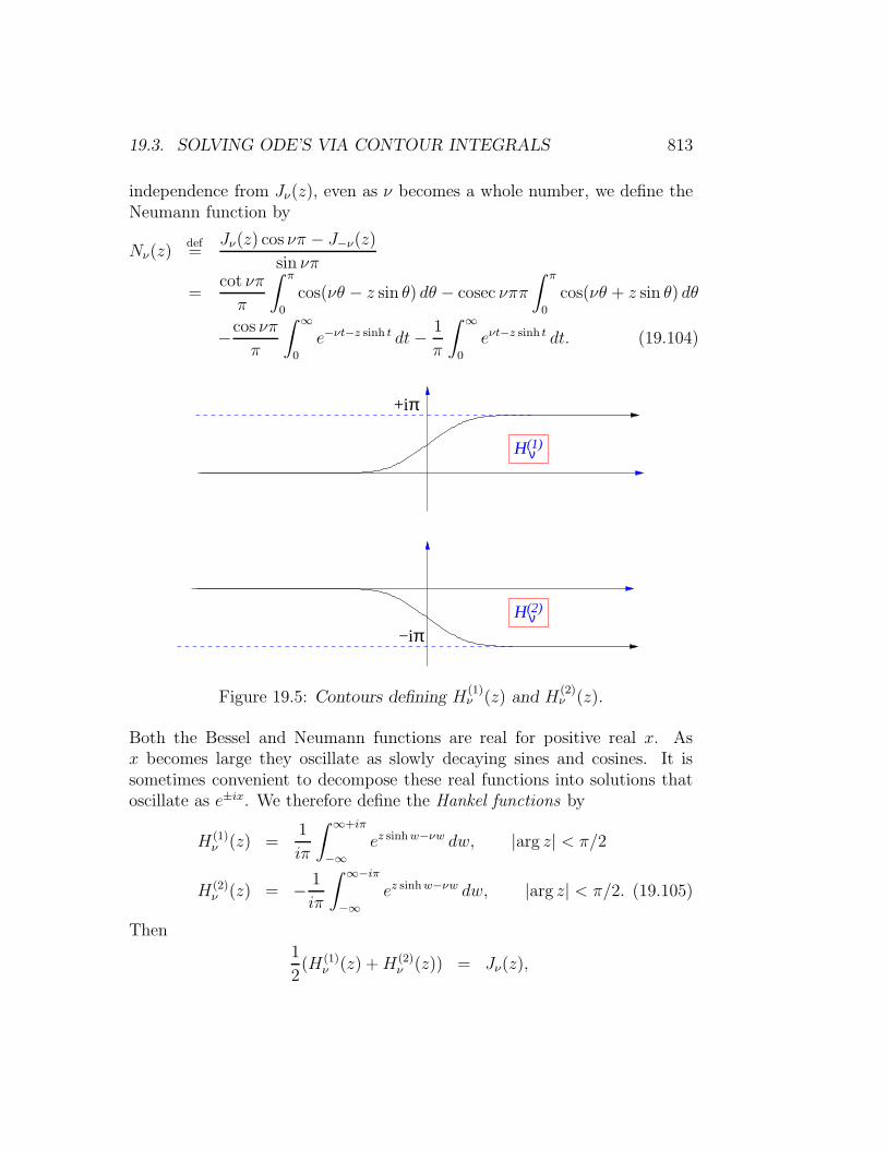
19.3. SOLVING ODE’S VIA CONTOUR INTEGRALS 813
independence from Jν(z), even as ν becomes a whole number, we define theNeumann function by
Nν(z)def=
Jν(z) cos νπ − J−ν(z)sin νπ
=cot νπ
π
∫ π
0
cos(νθ − z sin θ) dθ − cosec νππ
∫ π
0
cos(νθ + z sin θ) dθ
−cos νππ
∫ ∞
0
e−νt−z sinh t dt− 1
π
∫ ∞
0
eνt−z sinh t dt. (19.104)
+iπ
π−iHν
Hν
(2)
(1)
Figure 19.5: Contours defining H(1)ν (z) and H
(2)ν (z).
Both the Bessel and Neumann functions are real for positive real x. Asx becomes large they oscillate as slowly decaying sines and cosines. It issometimes convenient to decompose these real functions into solutions thatoscillate as e±ix. We therefore define the Hankel functions by
H(1)ν (z) =
1
iπ
∫ ∞+iπ
−∞ez sinhw−νw dw, |arg z| < π/2
H(2)ν (z) = − 1
iπ
∫ ∞−iπ
−∞ez sinhw−νw dw, |arg z| < π/2. (19.105)
Then1
2(H(1)
ν (z) +H(2)ν (z)) = Jν(z),

814CHAPTER 19. SPECIAL FUNCTIONS AND COMPLEX VARIABLES
1
2(H(1)
ν (z)−H(2)ν (z)) = Nν(z). (19.106)
19.4 Asymptotic Expansions
We often need the understand the behaviour of solutions of differential equa-tions and functions, such as Jν(x), when x takes values that are very large,or very small. This is the subject of asymptotics .
As an introduction to this art, consider the function
Z(λ) =
∫ ∞
−∞e−x
2−λx4 dx. (19.107)
Those of you who have taken a course quantum field theory based on pathintegrals will recognize that this is a “toy,” 0-dimensional, version of the pathintegral for the λϕ4 model of a self-interacting scalar field. Suppose we wishto obtain the perturbation expansion for Z(λ) as a power series in λ. Wenaturally proceed as follows
Z(λ) =
∫ ∞
−∞e−x
2−λx4 dx
=
∫ ∞
−∞e−x
2
∞∑
n=0
(−1)nλnx4n
n!dx
?=
∞∑
n=0
(−1)nλn
n!
∫ ∞
−∞e−x
2
x4n dx
=
∞∑
n=0
(−1)nλn
n!Γ(2n+ 1/2). (19.108)
Something has clearly gone wrong here! The gamma function Γ(2n+1/2) ∼(2n)! ∼ 4n(n!)2 overwhelms the n! in the denominator, so the radius ofconvergence of the final power series is zero.
The invalid, but popular, manœuvre is the interchange of the order ofperforming the integral and the sum. This interchange cannot be justifiedbecause the sum inside the integral does not converge uniformly on the do-main of integration. Does this mean that the series is useless? It had betternot! All quantum field theory (and most quantum mechanics) perturbationtheory relies on versions of this manœuvre.

19.4. ASYMPTOTIC EXPANSIONS 815
We are saved to some (often adequate) degree because, while the inter-change of integral and sum does not lead to a convergent series, it does leadto a valid asymptotic expansion. We write
Z(λ) ∼∞∑
n=0
(−1)nλn
n!Γ(2n+ 1/2) (19.109)
where
Z(λ) ∼∞∑
n=0
anλn (19.110)
is shorthand for the more explicit
Z(λ) =N∑
n=0
anλn +O
(λN+1
), N = 1, 2, 3, . . . . (19.111)
The “big O” notation,
Z(λ)−N∑
n=0
anλn = O(λN+1) (19.112)
as λ→ 0, means that
limλ→0
|Z(λ)−∑N
0 anλn|
|λN+1|
= K <∞. (19.113)
The basic idea is that, given a convergent power series∑
n anλn for the
function f(λ), we fix the value of λ and take more and more terms. Thesum then gets closer to f(λ). Given an asymptotic series, on the other hand,we select a fixed number of terms in the series and then make λ smaller andsmaller. The graph of f(λ) and the graph of our polynomial approximationthen approach each other. The more terms we take, the sooner they getclose, but for any non-zero λ we can never get exacty f(λ)—no matter howmany terms we take.
We often consider asymptotic expansions where the independent variablebecomes large. Here we have expansions in inverse powers of x:
F (x) =
N∑
n=0
bnx−n +O
(x−N−1
), N = 1, 2, 3 . . . . (19.114)

816CHAPTER 19. SPECIAL FUNCTIONS AND COMPLEX VARIABLES
In this case
F (x)−N∑
n=0
bnx−n = O
(x−N−1
)(19.115)
means that
limx→∞
|F (x)−∑N
0 bnx−n|
|x−N−1|
= K <∞. (19.116)
Again we take a fixed number of terms, and as x becomes large the functionand its approximation get closer.
Observations:i) Knowledge of the asymptotic expansion gives us useful knowledge about
the function, but does not give us everything. In particular, two distinctfunctions may have the same asymptotic expansion. For example, forsmall positive λ, the functions F (λ) and F (λ)+ae−b/λ have exactly thesame asymptotic expansions as series in positive powers of λ. This isbecause e−b/λ goes to zero faster than any power of λ, and so its asymp-totic expansion
∑n anλ
n has every coefficient an being zero. Physicistscommonly say that e−b/λ is a non-perturbative function, meaning thatit will not be visible to a perturbation expansion in powers of λ.
ii) An asymptotic expansion is usually valid only in a sector a < arg z < bin the complex plane. Different sectors have different expansions. Thisis called the Stokes’ phenomenon.
The most useful methods for obtaining asymptotic expansions requirethat the function to be expanded be given in terms of an integral. Thisis the reason why we have stressed the contour-integral method of solvingdifferential equations. If the integral can be approximated by a Gaussian, weare lead to the method of steepest descents . This technique is best explainedby means of examples.
19.4.1 Stirling’s approximation for n!
We start from the integral representation of the Gamma: function
Γ(x+ 1) =
∫ ∞
0
e−ttx dt (19.117)
Set t = xζ , so
Γ(x+ 1) = xx+1
∫ ∞
0
ezxf(ζ) dζ, (19.118)

19.4. ASYMPTOTIC EXPANSIONS 817
wheref(ζ) = ln ζ − ζ. (19.119)
We are going to be interested in evaluating this integral in the limit thatx→∞ and finding the first term in the asymptotic expansion of Γ(x+1) inpowers of 1/x. In this limit, the exponential will be dominated by the partof the integration region near the absolute maximum of f(ζ). Now, f(ζ) isa maximum at ζ = 1 and
f(ζ) = −1− 1
2(ζ − 1)2 + · · · . (19.120)
So
Γ(x+ 1) = xx+1e−x∫ ∞
0
e−x2(ζ−1)2+··· dζ
≈ xx+1e−x∫ ∞
−∞e−
x2(ζ−1)2 dζ
= xx+1e−x√
2π
x
=√2π xx+1/2e−x. (19.121)
By keeping more of the terms represented by the dots, and expandingthem as
e−x2(ζ−1)2+··· = e−
x2(ζ−1)2
[1 + a1(ζ − 1) + a2(ζ − 1)2 + · · ·
], (19.122)
we would find, on doing the integral, that
Γ(z+1) ≈√2πxx+1/2e−x
[1 +
1
12x+
1
288x2− 139
51840x3− 571
24888320x4+O
(1
x5
)].
(19.123)Since Γ(n+ 1) = n! we have the useful result
n! ≈√2πnn+1/2e−n
[1 +
1
12n+ · · ·
]. (19.124)
We make contact with our discusion of asymptotic series by rewriting theexpansion as
Γ(x+ 1)√2πxx+1/2e−x
∼ 1 +1
12x+
1
288x2− 139
51840x3− 571
24888320x4+ . . . (19.125)
This is typical. We usually have to pull out a leading factor from the functionwhose asymptotic behaviour we are studying, before we are left with a plainasymptotic power series.

818CHAPTER 19. SPECIAL FUNCTIONS AND COMPLEX VARIABLES
19.4.2 Airy functions
The Airy functions Ai(x) and Bi(x) are closely related to Bessel functions,and are named after the mathematician and astronomer George Biddell Airy.They occur widely in physics. We will investigate the behaviour of Ai(x) forlarge values of |x|. A more sophisticated treatment is needed for this problem,and we will meet with Stokes’ phenomenon. Airy’s differential equation is
d2y
dz2− zy = 0. (19.126)
On the real axis Airy’s equation becomes
−d2y
dx2+ xy = 0, (19.127)
and we we can think of this as the Schrodinger equation for a particle runningup a linear potential. A classical particle incident from the left with totalenergy E = 0 will come to rest at x = 0, and then retrace its path. The pointx = 0 is therefore called a classical turning point .The corresponding quantumwavefunction, Ai (x), contains a travelling wave incident from the left andbecoming evanescent as it tunnels into the classically forbidden region, x > 0,together with a reflected wave returning to −∞. The sum of the incidentand reflected waves is a real-valued standing wave.
-10 -5 5 10
-0.4
-0.2
0.2
0.4
Figure 19.6: The Airy function Ai (x).
We will look for contour integral solutions to Airy’s equation of the form
y(x) =
∫
C
extf(t) dt. (19.128)
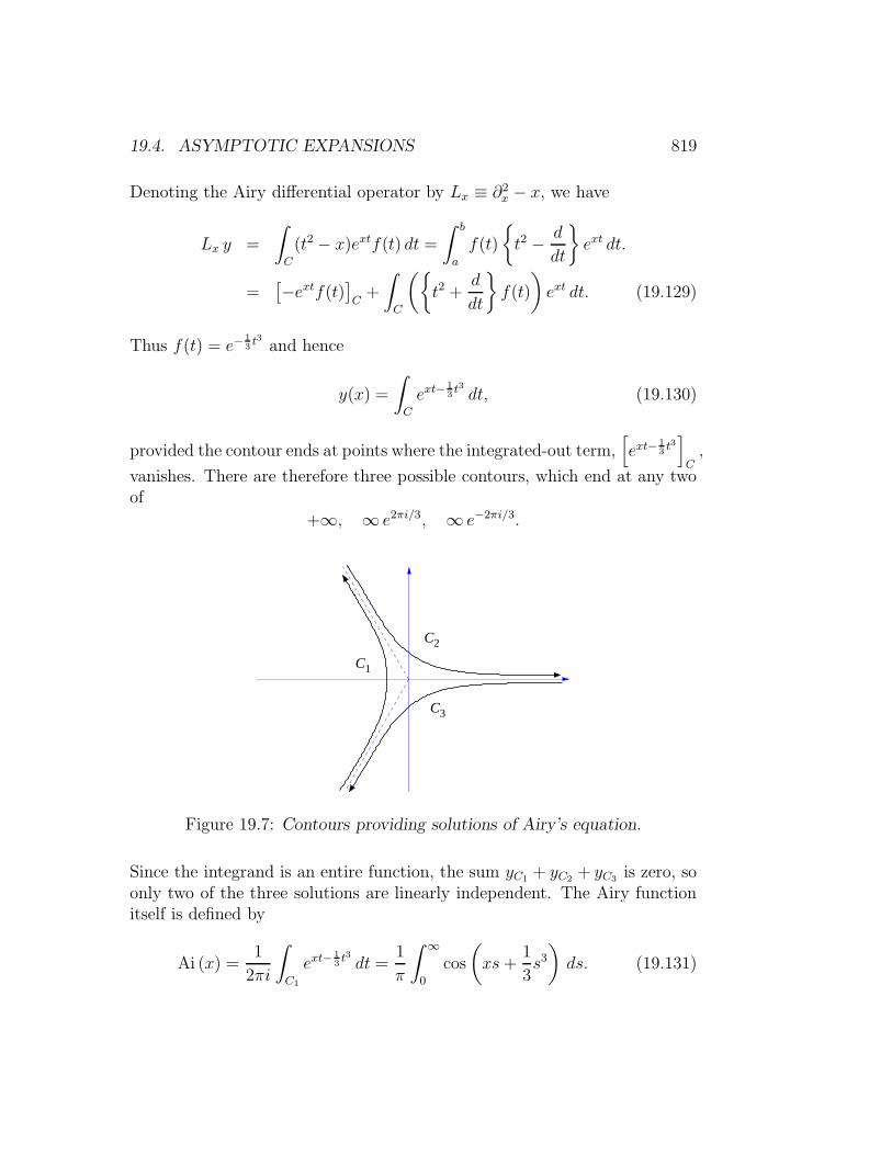
19.4. ASYMPTOTIC EXPANSIONS 819
Denoting the Airy differential operator by Lx ≡ ∂2x − x, we have
Lx y =
∫
C
(t2 − x)extf(t) dt =∫ b
a
f(t)
t2 − d
dt
ext dt.
=[−extf(t)
]C+
∫
C
(t2 +
d
dt
f(t)
)ext dt. (19.129)
Thus f(t) = e−13t3 and hence
y(x) =
∫
C
ext−13t3 dt, (19.130)
provided the contour ends at points where the integrated-out term,[ext−
13t3]C,
vanishes. There are therefore three possible contours, which end at any twoof
+∞, ∞ e2πi/3, ∞ e−2πi/3.
C1
C
C
2
3
Figure 19.7: Contours providing solutions of Airy’s equation.
Since the integrand is an entire function, the sum yC1+ yC2
+ yC3is zero, so
only two of the three solutions are linearly independent. The Airy functionitself is defined by
Ai (x) =1
2πi
∫
C1
ext−13t3 dt =
1
π
∫ ∞
0
cos
(xs+
1
3s3)ds. (19.131)

820CHAPTER 19. SPECIAL FUNCTIONS AND COMPLEX VARIABLES
In obtaining last equality, we have deformed the contour of integration, C1,which ran from ∞ e−2πi/3 to ∞ e2πi/3, so that it lies on the imaginary axis,and there we have written t = is. You may check (by extending Jordan’slemma) that this deformation does not alter the value of the integral.
To study the asymptotics of this function we need to examine separatelytwo cases x≫ 0 and x≪ 0. For both ranges of x, the principal contributionto the integral will come from the neighbourhood of the stationary pointsof f(t) = xt − t3/3. In the complex plane, stationary points are never puremaxima or minima of the real part of f (the real part alone determinesthe magnitude of the integrand) but are always saddle points . We mustdeform the contour so that on the integration path the stationary point isthe highest point in a mountain pass. We must also ensure that everywhereon the contour the difference between f and its maximum value stays real .Because of the orthogonality of the real and imaginary part contours, thismeans that we must take a path of steepest descent from the pass — hencethe name of the method. If we stray from the steepest descent path, thephase of the exponent will be changing. This means that the integrand willoscillate and we can no longer be sure that the result is dominated by thecontributions near the saddle point.
b)a)
u
v v
u
Figure 19.8: Steepest descent contours, location of the stationary points andorientation of the saddle passes for a) x≫ 0, b) x≪ 0.
i) x≫ 0 : The stationary points are at t = ±√x. Writing t = ξ −√x have
f(ξ) = −23x3/2 + ξ2
√x− 1
3ξ3 (19.132)

19.4. ASYMPTOTIC EXPANSIONS 821
while near t = +√x we write t = ζ +
√x and find
f(ζ) = +2
3x3/2 − ζ2√x− 1
3ζ3 (19.133)
We see that the saddle point near −√x is a local maximum when weroute the contour vertically, while the saddle point near +
√x is a local
maximum as we go down the real axis. Since the contour in Ai (x) isaimed vertically we can distort it to pass through the saddle point near−√x, but cannot find a route through the point at +
√x without the
integrand oscillating wildly. At the saddle point the exponent, xt−t3/3,is real. If we write t = u+ iv we have
Im (xt− t3/3) = v(x− u2 + v2/3), (19.134)
so the exact steepest descent path, on which the imaginary part remainszero is given by the union of real axis (v = 0) and the curve
u2 − 1
3v2 = x. (19.135)
This is a hyperbola, and the branch passing through the saddle pointat −√x is plotted in a).Now setting ξ = is, we find
Ai (x) =1
2πe−
23x3/2
∫ ∞
−∞e−
√xs2+··· ds ∼ 1
2√πx−1/4e−
23x3/2 . (19.136)
ii) x≪ 0 : The stationary points are now at ±i√|x|. Setting t = ξ ± i
√|x|
find that
f(x) = ∓i23|x|3/2 ∓ iξ2
√|x|. (19.137)
The exponent is no longer real, but the imaginary part will be constantand the integrand non-oscillatory provided we deform the contour sothat it becomes the disconnected pair of curves shown in b). Thenew contour passes through both saddle points and we must sum theircontributions. Near t = i
√|x| we set ξ = e3πi/4s and get
1
2πie3πi/4e−i
23|x|3/2
∫ ∞
−∞e−√
|x|s2 ds =1
2i√πe3πi/4|x|−1/4e−i
23|x|3/2
= − 1
2i√πe−iπ/4|x|−1/4e−i
23|x|3/2
(19.138)

822CHAPTER 19. SPECIAL FUNCTIONS AND COMPLEX VARIABLES
Near t = −i√|x|we set ξ = eπi/4s and get
1
2πieπi/4ei
23|x|3/2
∫ ∞
−∞e−√
|x|s2 ds =1
2i√πeπi/4|x|−1/4ei
23|x|3/2 (19.139)
The sum of these two contributions is
Ai (x) ∼ 1√π|x|1/4 sin
(2
3|x|3/2 + π
4
). (19.140)
The fruit of our labours is therefore
Ai (x) ∼ 1
2√πx−1/4e−
23x3/2[1 +O
(1
x
)], x > 0,
∼ 1√π|x|1/4 sin
(2
3|x|3/2 + π
4
)[1 + O
(1
x
)], x < 0.
(19.141)
Suppose that we allow x to become complex x → z = |z|eiθ, with −π <θ < π. Then figure 19.9 shows how the steepest contour evolves and leadsthe two quite different expansion for positive and negative x. We see thatfor 0 < θ < 2π/3 the steepest descent path continues to be routed throughthe single stationary point at −
√|z|eiθ/2. Once θ reaches 2π/3, though, it
passes through both stationary points. The contribution to the integral fromthe newly acquired stationary point is, however, exponentially smaller as|z| → ∞ than that of t = −
√|z|eiθ/2. The new term is therefore said to
be subdominant , and makes an insignificant contribution to the asymptoticbehaviour of Ai (z). The two saddle points only make contributions of thesame magnitude when θ reaches π. If we analytically continue beyond θ = π,the new saddle point will now dominate over the old, and only its contribtionis significant at large |z|. The Stokes line, at which we must change the formof the asymptotic expansion is therefore at θ = π.
If we try to systematically keep higher order terms we will find, for theoscillating Ai (−z), a double series
Ai (−z) ∼ π−1/2z−1/4
[sin(ρ+ π/4)
∞∑
n=0
(−1)nc2nρ−2n
− cos(ρ+ π/4)
∞∑
n=0
(−1)nc2n+1ρ−2n−1
](19.142)
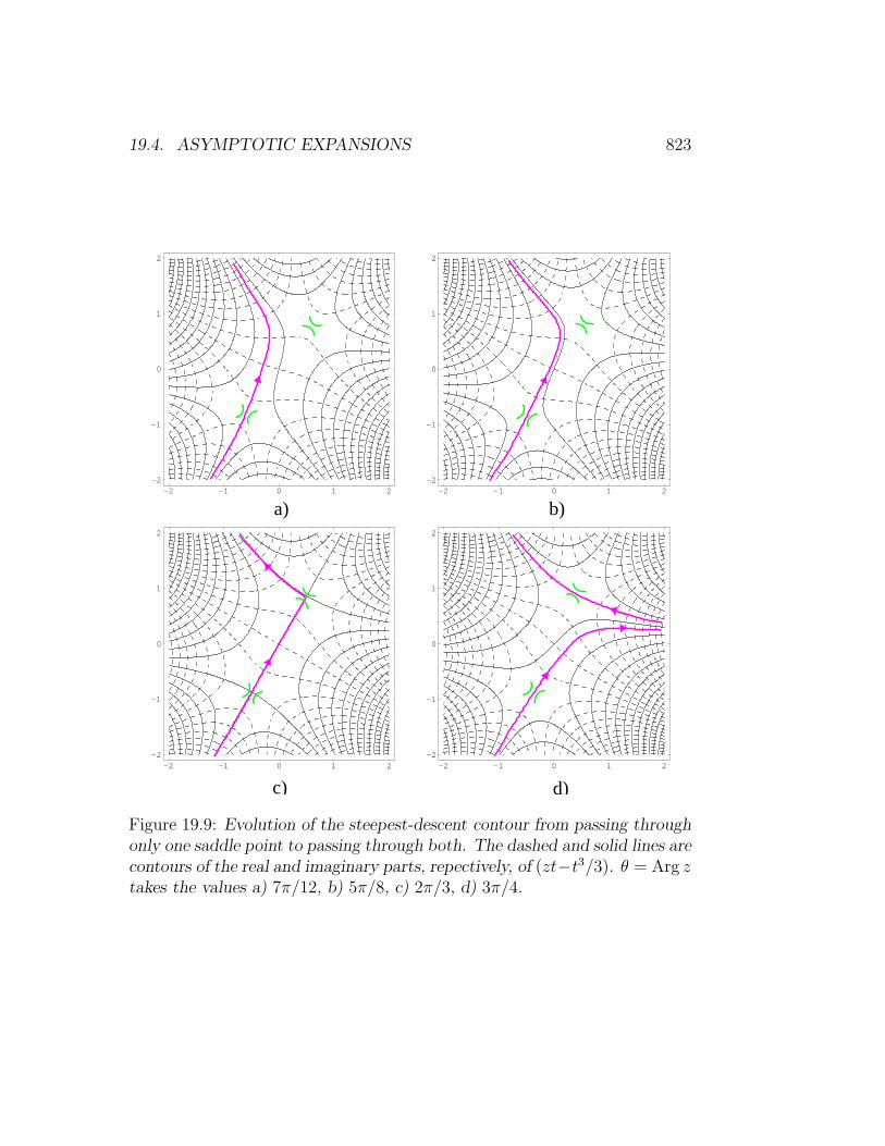
19.4. ASYMPTOTIC EXPANSIONS 823
-2 -1 0 1 2-2
-1
0
1
2
-2 -1 0 1 2-2
-1
0
1
2
-2 -1 0 1 2-2
-1
0
1
2
-2 -1 0 1 2-2
-1
0
1
2
a) b)
c) d)
Figure 19.9: Evolution of the steepest-descent contour from passing throughonly one saddle point to passing through both. The dashed and solid lines arecontours of the real and imaginary parts, repectively, of (zt−t3/3). θ = Arg ztakes the values a) 7π/12, b) 5π/8, c) 2π/3, d) 3π/4.
824CHAPTER 19. SPECIAL FUNCTIONS AND COMPLEX VARIABLES
where ρ = 2z3/2/3. In this case, therefore we need to extract two leadingcoefficients before we have asymptotic power series.
The subject of asymptotics contains many subtleties, and the reader insearch of a more detailed discussion is recommended to read Bender andOrszag’s Advanced Mathematical Methods for Scientists and Engineers .
Exercise 19.2: Consider the behaviour of Bessel functions when x is large. Byapplying the method of steepest descent to the Hankel function contours showthat
H(1)ν (x) ∼
√2
πxei(x−νπ/2−π/4)
[1− 4ν2 − 1
8πx+ · · ·
]
H(2)ν (x) ∼
√2
πxe−i(x−νπ/2−π/4)
[1 +
4ν2 − 1
8πx+ · · ·
],
and hence
Jν(x) ∼√
2
πx
[cos(x− νπ
2− π
4
)− 4ν2 − 1
8xsin(x− νπ
2− π
4
)+ · · ·
],
Nν(x) ∼√
2
πx
[sin(x− νπ
2− π
4
)+
4ν2 − 1
8xcos(x− νπ
2− π
4
)+ · · ·
].
19.5 Elliptic Functions
The subject of elliptic functions goes back to remarkable identities of GuilioFagnano (1750) and Leonhard Euler (1761). Euler’s formula is
∫ u
0
dx√1− x4
+
∫ v
0
dy√1− y4
=
∫ r
0
dz√1− z4
, (19.143)
where 0 ≤ u, v ≤ 1, and
r =u√1− v4 + v
√1− u4
1 + u2v2. (19.144)
This looks mysterious, but perhaps so does∫ u
0
dx√1− x2
+
∫ v
0
dy√1− y2
=
∫ r
0
dz√1− z2
, (19.145)
wherer = u
√1− v2 + v
√1− u2, (19.146)

19.5. ELLIPTIC FUNCTIONS 825
until you realize that the latter formula (19.146) is merely
sin(a+ b) = sin a cos b+ cos a sin b (19.147)
in disguise. To see this set
u = sin a, v = sin b (19.148)
and remember the integral formula for the inverse trigonometric sine function
a = sin−1 u =
∫ u
0
dx√1− x2
. (19.149)
The Fagnano-Euler formula is a similarly-disguised addition formula for anelliptic function. Just as we use the substitution x = sin y in the 1/
√1− x2
integral, we can use an elliptic-function substitution to evaluate elliptic inte-grals which involve square-roots of quartic or cubic polynomials. Examplesare
I4 =
∫ x
0
dt√(t− a1)(t− a2)(t− a3)(t− a4)
, (19.150)
I3 =
∫ x
0
dt√(t− a1)(t− a2)(t− a3)
. (19.151)
Note that I4 can be reduced to an integral of the form I3 by using a Mobius-map substitution
t =at′ + b
ct′ + d, dt = (ad− bc) dt′
(ct′ + d)2(19.152)
to send a4 to infinity. Indeed, we can use a suitable Mobius map to send anythree of the four points an to 0, 1,∞.
The idea of elliptic functions (as opposed to elliptic integrals , which aretheir functional inverses) was known to Gauss, but Abel and Jacobi were thefirst to publish (1827). For the developing the general theory, the simplestelliptic function is the Weierstrass ℘. This is really a family of functions thatis parametrized by a pair of linearly independent complex numbers or periodsω1, ω2. For a given pair of periods, the ℘ function is defined by the doublesum
℘(z) =1
z2+
∑
(m,n)6=(0,0)
1
(z −mω1 − nω2)2− 1
(mω1 + nω2)2
. (19.153)

826CHAPTER 19. SPECIAL FUNCTIONS AND COMPLEX VARIABLES
Helped by the counterterm, the sum is absolutely convergent, so we canrearrange the terms to prove double periodicity
℘(z +mω1 + nω2) = ℘(z), m, n ∈ Z. (19.154)
The function is thus determined everywhere by its values in the period paral-lelogram P = λω1 + µω2 : 0 ≤ λ, µ < 1. Double periodicity is the definingcharacteristic of elliptic functions.
.
.
.
.
.
.
.
.
ω
ω2
x
y
1
.
.
Figure 19.10: Unit cell and double-periodicity.
Any non-constant meromorphic function f(z) that is doubly periodic hasfour basic properties:
a) The function must have at least one pole in its unit cell. Otherwiseit would be holomorphic and bounded, and therefore a constant byLiouville.
b) The sum of the residues at the poles must add to zero. This followsfrom integrating f(z) around the boundary of the period parallelogramand observing that the contributions from opposite edges cancel.
c) The number of poles in each unit cell must equal the number of zeros.This follows from integrating f ′/f around the boundary of the periodparallelogram.
d) If f has zeros at the N points zi and poles at the N points pi then
N∑
i=1
zi −N∑
i=1
pi = nω1 +mω2
where m,n are integers. This follows from integrating zf ′/f aroundthe boundary of the period parallelogram.

19.5. ELLIPTIC FUNCTIONS 827
The Weierstrass ℘ has a second-order pole at the origin. It also obeys
lim|z|→0
(℘(z)− 1
z2
)= 0,
℘(z) = ℘(−z),℘′(z) = −℘′(−z). (19.155)
The property that makes ℘(z) useful for evaluating integrals is
(℘′(z))2= 4℘3(z)− g2℘(z)− g3, (19.156)
where
g2 = 60∑
(m,n)6=(0,0)
1
(mω1 + nω2)4, g3 = 140
∑
(m,n)6=(0,0)
1
(mω1 + nω2)6.
(19.157)Equation (19.156) is proved by examining the first few terms in the Laurentexpansion in z of the difference of the left hand and right hand sides. Allnegative powers cancel, as does the constant term. The difference is zero atz = 0, has no poles or other singularities, and, being continuous and peri-odic, is automatically bounded. It is therefore identically zero by Liouville’stheorem.
From the symmetry and periodicity of ℘ we see that ℘′(z) = 0 at ω1/2,ω2/2 and (ω1+ω2)/2 where ℘(z) takes the values e1 = ℘(ω1/2), e2 = ℘(ω2/2),and e3 = ℘((ω1+ω2)/2). Now ℘′ must have exactly three zeros since it has apole of order three at the origin and, by property c), the number of zeros inthe unit cell is equal to the number of poles. We therefore know the locationof all three zeros, and can factorize:
4℘3(z)− g2℘(z)− g3 = 4(℘− e1)(℘− e2)(℘− e3). (19.158)
We note that the coefficient of ℘2 in the polynomial on the left side is zero,implying that e1 + e2 + e3 = 0.
The roots ei can never coincide. For example, (℘(z) − e1) has a doublezero at ω1/2, but two zeros is all it is allowed because the number of polesper unit cell equals the number of zeros, and (℘(z)− e1) has a double pole at0 as its only singularity. Thus, (℘− e1) cannot be zero at another point, butit would be if e1 coincided with e2 or e3. As a consequence, the discriminant
∆def= 16(e1 − e2)2(e2 − e3)2(e1 − e3)2 = g32 − 27g23, (19.159)
828CHAPTER 19. SPECIAL FUNCTIONS AND COMPLEX VARIABLES
is never zero.We use ℘ and (19.156) to write
z = ℘−1(u) =
∫ u
∞
dt
2√(t− e1)(t− e2)(t− e3)
=
∫ u
∞
dt√4t3 − g2t− g3
.
(19.160)This maps the u plane, with cuts that we can take from e1 to e2 and e3 to∞,one-to-one onto the 2-torus, regarded the unit cell of the ωn,m = nω1 +mω2
lattice.As z sweeps over the torus, the points x = ℘(z), y = ℘′(z) move on the
elliptic curvey2 = 4x3 − g2x− g3 (19.161)
which should be thought of as a set in CP 2. These curves, and the finite fieldsof rational points that lie on them, are exploited in modern cryptography.
The magic that leads to addition formula, such as the Euler-Fagnano re-lation (19.144) with which we began this section, lies in the (not immediatleyobvious) fact that any elliptic function having the same periods as ℘(z) canbe expressed as a rational function of ℘(z) and ℘′(z). From this it follows(after some thought) that any two such elliptic functions, f1(z) and f2(z),obey a relation F (f1, f2) = 0, where
F (x, y) =∑
m,n
an,mxnym (19.162)
is a polynomial in x and y. We can eliminate ℘′(z) in these relations bywriting ℘′(z) =
√4℘3(z)− g2℘(z)− g3.
Modular invariance
If ω1 and ω2 are periods and define a unit cell, so are
ω′1 = aω1 + bω2
ω′2 = cω1 + dω2
where a, b, c, d are integers with ad − bc = ±1. This condition on the deter-minant ensures that the matrix inverse also has integer entries, and so the ωican be expressed in terms of the ω′
i with integer coefficients. Consequentlythe set of integer linear combinations of the ω′
i generate the same lattice asthe integer linear combinations of the original ωi. This notion of redefining

19.5. ELLIPTIC FUNCTIONS 829
the unit cell should be familiar to you from solid state physics. If we wishto preserve the orientation of the basis vectors, we must restrict ourselvesto maps whose determinant ad − bc is unity. The set of such transformsconstitute the the modular group SL(2,Z). Clearly ℘ is invariant under thisgroup, as are g2 and g3 and ∆. Now define ω2/ω1 = τ , and write
g2(ω1, ω2) =1
ω41
g2(τ), g3(ω1, ω2) =1
ω61
g3(τ). ∆(ω1, ω2) =1
ω121
∆(τ),
(19.163)and also
J(τ) =g32
g32 − 27g23=g32∆. (19.164)
Because the denominator is never zero when Im τ > 0, the function J(τ) isholomorphic in the upper half-plane — but not on the real axis. The functionJ(τ) is called the elliptic modular function.
Except for the prefactors ωn1 , the functions gi(τ), ∆(τ) and J(τ) areinvariant under the Mobius transformation
τ → aτ + b
cτ + d, (19.165)
with (a bc d
)∈ SL(2,Z). (19.166)
This Mobius transformation does not change if the entries in the matrix aremultiplied by a common factor of±1, and so the transformation is an elementof the modular group PSL(2,Z) ≡ SL(2,Z)/I,−I.
Taking into account the change in the ωα1 prefactors we have
g2
(aτ + b
cτ + d
)= (cτ + d)4g3(τ),
g3
(aτ + b
cτ + d
)= (cτ + d)6g3(τ),
∆
(aτ + b
cτ + d
)= (cτ + d)12∆(τ). (19.167)
Because c = 0 and d = 1 for the special case τ → τ +1, these three functionsobey f(τ+1) = f(τ) and so depend on τ only via the combination q2 = e2πiτ .

830CHAPTER 19. SPECIAL FUNCTIONS AND COMPLEX VARIABLES
For example, it is not hard to prove that
∆(τ) = (2π)12q2∞∏
n=1
(1− q2n
)24. (19.168)
We can also expand these functions as power series in q2 — and here thingsget interesting because the coefficients have number-theoretic properties. Forexample
g2(τ) = (2π)4
[1
12+ 20
∞∑
n=1
σ3(n)q2n
],
g3(τ) = (2π)6
[1
216− 7
3
∞∑
n=1
σ5(n)q2n
]. (19.169)
The symbol σk(n) is defined by σk(n) =∑d k, where d runs over all positive
divisors of the number n.In the case of the function J(τ), the prefactors cancel and
J
(aτ + b
cτ + d
)= J(τ), (19.170)
so J(τ) is a modular invariant . One can show that if J(τ1) = J(τ2), then
τ2 =aτ1 + b
cτ1 + d(19.171)
for some modular transformation with integer a, b, c, d, where ad − bc = 1,and further, that any modular-invariant function is a rational function ofJ(τ). It seems clear that J(τ) is rather a special object.
This J(τ) is the function referred to on page 560 in connection with theMonster group. As with the gi, J(τ) depends on τ only through q2. The firstfew terms in the power series expansion of J(τ) in terms of q2 turn out to be
1728J(τ) = q−2+744+196884q2+21493760q4+864299970q6+· · · . (19.172)
Since AJ(τ)+B has all the same modular invariance properties as J(τ), thenumbers 1728 (= 123) and 744 are just conventional normalizations. Once weset the coefficient of q−2 to unity, however, the remaining integer coefficientsare completely determined by the modular properties. A number-theory

19.6. FURTHER EXERCISES AND PROBLEMS 831
interpretation of these integers seemed lacking until John McKay and othersobserved that
1 = 1
196884 = 1 + 196883
21493760 = 1 + 196883 + 21296786
864299970 = 2×1 + 2×196883 + 21296786 + 842609326,
(19.173)
where “1” and the large integers on the right-hand side are the dimensions ofthe smallest irreducible representations of the Monster. This “MonstrousMoonshine” was originally mysterious and almost unbelievable, (“moon-shine” = “fantastic nonsense”) but it was explained by Richard Borcherdsby the use of techniques borrowed from string theory.3 Borcherds receivedthe 1998 Fields Medal for this work.
19.6 Further Exercises and Problems
Exercise 19.3: Show that the binomial series expansion of (1 + x)−ν can bewritten as
(1 + x)−ν =∞∑
m=0
(−x)mΓ(m+ ν)
Γ(ν)m!, |x| < 1.
Exercise 19.4: A Mellin transform and its inverse. Combine the Beta-functionidentity (19.15) with a suitable change of variables to evaluate the Mellintransform ∫ ∞
0xs−1(1 + x)−ν dx, ν > 0,
of (1 + x)−ν as a product of Gamma functions. Now consider the Bromwichcontour integral
1
2πiΓ(ν)
∫ c+i∞
c−i∞x−sΓ(ν − s)Γ(s) ds.
3“I was in Kashmir. I had been traveling around northern India, and there was onereally long tiresome bus journey, which lasted about 24 hours. Then the bus had to stopbecause there was a landslide and we couldn’t go any further. It was all pretty darnunpleasant. Anyway, I was just toying with some calculations on this bus journey andfinally I found an idea which made everything work”- Richard Borcherds (Interview inThe Guardian, August 1998).

832CHAPTER 19. SPECIAL FUNCTIONS AND COMPLEX VARIABLES
Here Re c ∈ (0, ν). The Bromwich contour therefore runs parallel to the imag-inary axis with the poles of Γ(s) to its left and the poles of Γ(ν − s) to itsright. Use the identity
Γ(s)Γ(1− s) = π cosec πs
to show that when |x| < 1 the contour can be closed by a large semicircle lyingto the left of the imaginary axis. By using the preceding exercise to sum thecontributions from the enclosed poles at s = −n, evaluate the integral.
Exercise 19.5: Mellin-Barnes integral. Use the technique developed in thepreceding exercise to show that
F (a, b, c;−x) = Γ(c)
2πiΓ(a)Γ(b)
∫ c+i∞
c−i∞x−s
Γ(a− s)Γ(b− s)Γ(s)Γ(c− s) ds,
for a suitable range of x. This integral representation of the hypergeometricfunction is due to the English mathematician Ernest Barnes (1908), later acontroversial Bishop of Birmingham.
Exercise 19.6: Let
Y =
(y1y2
)
Show that the matrix differential equation
d
dxY =
A
zY +
B
1− zY,
where
A =
(0 a0 1− c
), B =
(0 0b a+ b− c+ 1
),
has a solution
Y (z) = F (a, b; c; z)
(10
)+z
aF ′(a, b; c; z)
(01
).
Exercise 19.7: Kniznik-Zamolodchikov equation. The monodromy propertiesof solutions of differential equations play an important role in conformal fieldtheory. The Fuchsian equations studied in this exercise are obeyed by thecorrelation functions in the level-k Wess-Zumino-Witten model.
Let V (a), a = 1, . . . n, be spin-ja representation spaces for the group SU(2). LetW (z1, . . . , zn) be a function taking values in V (1)⊗V (2)⊗· · ·⊗V (n). (In other

19.6. FURTHER EXERCISES AND PROBLEMS 833
words W is a function Wi1,...,in(z1, . . . , zn) where the index ia labels states inthe spin-ja factor.) Suppose that W obeys the Kniznik-Zamolodchikov (K-Z)equations
(k + 2)∂
∂zaW =
∑
b,b6=a
J(a) · J(b)
za − zbW, a = 1, . . . , n,
whereJ(a) · J(b) ≡ J (a)
1 J(b)1 + J
(a)2 J
(b)2 + J
(a)3 J
(b)3 ,
and J(a)i indicates the su(2) generator Ji acting on the V (a) factor in the tensor
product. If we set z1 = z, for example and fix the position of z2, . . . zn, thenthe differential equation in z has regular singular points at the n−1 remainingzb.
a) By diagonalizing the operator J(a) · J(b) show that there are solutionsW (z) that behave for za close to zb as
W (z) ∼ (za − zb)∆j−∆ja−∆jb ,
where
∆j =j(j + 1)
k + 2, ∆ja =
ja(ja + 1)
k + 2,
and j is one of the spins |ja− jb| ≤ j ≤ j1 + ja occuring in the decompo-sition of ja ⊗ jb.
b) Define covariant derivatives
∇a =∂
∂za−∑
b,b6=a
J(a) · J(b)
za − zb
and show that [∇a,∇b] = 0. Conclude that the effect of parallel transportof the solutions of the K-Z equations provides a representation of thebraid group of the world lines of the za.

834CHAPTER 19. SPECIAL FUNCTIONS AND COMPLEX VARIABLES

Appendix A
Linear Algebra Review
In physics we often have to work with infinite dimensional vector spaces.Navigating these vasty deeps is much easier if you have a sound grasp of thetheory of finite dimensional spaces. Most physics students have studied thisas undergraduates, but not always in a systematic way. In this appendixwe gather together and review those parts of linear algebra that we will finduseful in the main text.
A.1 Vector Space
A.1.1 Axioms
A vector space V over a field F is a set equipped with two operations: abinary operation called vector addition which assigns to each pair of elementsx, y ∈ V a third element denoted by x+ y, and scalar multiplication whichassigns to an element x ∈ V and λ ∈ F a new element λx ∈ V . There is alsoa distinguished element 0 ∈ V such that the following axioms are obeyed:1
1) Vector addition is commutative: x + y = y + x.2) Vector addition is associative: (x+ y) + z = x+ (y + z).3) Additive identity: 0+ x = x.4) Existence of an additive inverse: for any x ∈ V , there is an element
(−x) ∈ V , such that x+ (−x) = 0.5) Scalar distributive law i) λ(x+ y) = λx+ λy.6) Scalar distributive law ii) (λ+ µ)x = λx+ µx.
1In this list 1, λ, µ,∈ F and x, y,0 ∈ V .
835

836 APPENDIX A. LINEAR ALGEBRA REVIEW
7) Scalar multiplicatiion is associative: (λµ)x = λ(µx).8) Multiplicative identity: 1x = x.
The elements of V are called vectors . We will only consider vector spacesover the field of the real numbers, F = R, or the complex numbers, F = C.
You have no doubt been working with vectors for years, and are saying toyourself “I know this stuff.” Perhaps so, but to see if you really understandthese axioms try the following exercise. Its value lies not so much in thesolution of its parts, which are easy, as in appreciating that these commonlyused properties both can and need to be proved from the axioms. (Hint:work the problems in the order given; the later parts depend on the earlier.)
Exercise A.1: Use the axioms to show that:
i) If x+ 0 = x, then 0 = 0.ii) We have 0x = 0 for any x ∈ V . Here 0 is the additive identity in F.iii) If x+ y = 0, then y = −x. Thus the additive inverse is unique.iv) Given x, y in V , there is a unique z such that x+z = y, to whit z = x−y.v) λ0 = 0 for any λ ∈ F.vi) If λx = 0, then either x = 0 or λ = 0.vii) (−1)x = −x.
A.1.2 Bases and components
Let V be a vector space over F. For the moment, this space has no additionalstructure beyond that of the previous section — no inner product and so nonotion of what it means for two vectors to be orthogonal. There is still muchthat can be done, though. Here are the most basic concepts and propertiesthat need to be understand:
i) A set of vectors e1, e2, . . . , en is linearly dependent if there exist λµ ∈F, not all zero, such that
λ1e1 + λ2e2 + · · ·+ λnen = 0. (A.1)
ii) If it is not linearly dependent, a set of vectors e1, e2, . . . , en is linearlyindependent . For a linearly independent set, a relation
λ1e1 + λ2e2 + · · ·+ λnen = 0 (A.2)
can hold only if all the λµ are zero.

A.1. VECTOR SPACE 837
iii) A set of vectors e1, e2, . . . , en is said to span V if for any x ∈ V thereare numbers xµ such that x can be written (not necessarily uniquely)as
x = x1e1 + x2e2 + · · ·+ xnen. (A.3)
A vector space is finite dimensional if a finite spanning set exists.iv) A set of vectors e1, e2, . . . , en is a basis if it is a maximal linearly
independent set (i.e. introducing any additional vector makes the setlinearly dependent). An alternative definition declares a basis to be aminimal spanning set (i.e. deleting any of the ei destroys the spanningproperty). Exercise: Show that these two definitions are equivalent.
v) If e1, e2, . . . , en is a basis then any x ∈ V can be written
x = x1e1 + x2e2 + . . . xnen, (A.4)
where the xµ, the components of the vector with respect to this basis,are unique in that two vectors coincide if and only if they have thesame components.
vi) Fundamental Theorem: If the sets e1, e2, . . . , en and f1, f2, . . . , fmare both bases for the space V then m = n. This invariant integer isthe dimension, dim (V ), of the space. For a proof (not difficult) seea mathematics text such as Birkhoff and McLane’s Survey of ModernAlgebra, or Halmos’ Finite Dimensional Vector Spaces.
Suppose that e1, e2, . . . , en and e′1, e′2, . . . , e′n are both bases, and that
eν = aµνe′µ. (A.5)
Since e1, e2, . . . , en is a basis, the e′ν can also be uniquely expressed in termsof the eµ, and so the numbers aµν constitute an invertible matrix. (Note thatwe are, as usual, using the Einstein summation convention that repeatedindices are to be summed over.) The components x′µ of x in the new basisare then found by comparing the coefficients of e′µ in
x′µe′µ = x = xνeν = xν(aµνe
′µ
)= (xνaµν ) e
′µ (A.6)
to be x′µ = aµνxν , or equivalently, xν = (a−1)νµ x
′µ. Note how the eµ and thexµ transform in “opposite” directions. The components xµ are therefore saidto transform contravariantly .

838 APPENDIX A. LINEAR ALGEBRA REVIEW
A.2 Linear Maps
Let V and W be vector spaces having dimensions n and m respectively. Alinear map, or linear operator , A is a function A : V → W with the propertythat
A(λx + µy) = λA(x) + µA(y). (A.7)
A.2.1 Matrices
The linear map A is an object that exists independently of any basis. Givenbases eµ for V and fν for W , however, the map may be represented byan m-by-n matrix . We obtain this matrix
A =
a11 a12 . . . a1na21 a22 . . . a2n...
.... . .
...am1 am2 . . . amn
, (A.8)
having entries aνµ, by looking at the action of A on the basis elements:
A(eµ) = fνaνµ . (A.9)
To make the right-hand-side of (A.9) look like a matrix product, where wesum over adjacent indices, the array aνµ has been written to the right of thebasis vector.2 The map y = A(x) is therefore
y ≡ yνfν = A(x) = A(xµeµ) = xµA(eµ) = xµ(fνaνµ) = (aνµx
µ)fν , (A.10)
whence, comparing coefficients of fν , we have
yν = aνµxµ. (A.11)
The action of the linear map on components is therefore given by the usualmatrix multiplication from the left : y = Ax, or more explicitly
y1
y2...ym
=
a11 a12 . . . a1na21 a22 . . . a2n...
.... . .
...am1 am2 . . . amn
x1
x2...xn
. (A.12)
2You have probably seen this “backward” action before in quantum mechanics. If weuse Dirac notation |n〉 for an orthonormal basis, and insert a complete set of states, |m〉〈m|,then A|n〉 = |m〉〈m|A|n〉. The matrix 〈m|A|n〉 representing the operator A operating ona vector from the left thus automatically appears to the right of the basis vectors used toexpand the result.

A.2. LINEAR MAPS 839
The identity map I : V → V is represented by the n-by-n matrix
In =
1 0 0 . . . 00 1 0 . . . 00 0 1 . . . 0...
......
. . ....
0 0 0 . . . 1
, (A.13)
which has the same entries in any basis.
Exercise A.2: Let U , V , W be vector spaces, and A : V → W , B : U → Vlinear maps which are represented by the matrices A with entries aµν and B
with entries bµν , respectively. Use the action of the maps on basis elementsto show that the map AB : U →W is represented by the matrix product AB
whose entries are aµλbλν .
A.2.2 Range-nullspace theorem
Given a linear map A : V → W , we can define two important subspaces:i) The kernel or nullspace is defined by
KerA = x ∈ V : A(x) = 0. (A.14)
It is a subspace of V .ii) The range or image space is defined by
ImA = y ∈ W : y = A(x),x ∈ V . (A.15)
It is a subspace of the target space W .The key result linking these spaces is the range-nullspace theorem whichstates that
dim (KerA) + dim (ImA) = dim V
It is proved by taking a basis nµ for KerA and extending it to a basis for thewhole of V by appending (dimV − dim (KerA)) extra vectors eν . It is easyto see that the vectors A(eν) are linearly independent and span ImA ⊆ W .Note that this result is meaningless unless V is finite dimensional.
The number dim (ImA) is the number of linearly independent columnsin the matrix, and is often called the (column) rank of the matrix.
840 APPENDIX A. LINEAR ALGEBRA REVIEW
A.2.3 The dual space
Associated with the vector space V is its dual space, V ∗, which is the set oflinear maps f : V → F. In other words the set of linear functions f( ) thattake in a vector and return a number. These functions are often also calledcovectors . (Mathematicians place the prefix co- in front of the name of amathematical object to indicate a dual class of objects, consisting of the setof structure-preserving maps of the original objects into the field over whichthey are defined.)
Using linearity we have
f(x) = f(xµeµ) = xµf(eµ) = xµ fµ. (A.16)
The set of numbers fµ = f(eµ) are the components of the covector f ∈ V ∗.If we change basis eν = aµνe
′µ then
fν = f(eν) = f(aµνe′µ) = aµνf(e
′µ) = aµνf
′µ. (A.17)
Thus fν = aµνf′µ and the fµ components transform in the same manner as the
basis. They are therefore said to transform covariantly .Given a basis eµ of V , we can define a dual basis for V ∗ as the set of
covectors e∗µ ∈ V ∗ such that
e∗µ(eν) = δµν . (A.18)
It should be clear that this is a basis for V ∗, and that f can be expanded
f = fµe∗µ. (A.19)
Although the spaces V and V ∗ have the same dimension, and are thereforeisomorphic, there is no natural map between them. The assignment eµ 7→ e∗µ
is unnatural because it depends on the choice of basis.One way of driving home the distinction between V and V ∗ is to consider
the space V of fruit orders at a grocers. Assume that the grocer stocks onlyapples, oranges and pears. The elements of V are then vectors such as
x = 3kg apples + 4.5kg oranges + 2kgpears. (A.20)
Take V ∗ to be the space of possible price lists, an example element being
f = (£3.00/kg) apples∗ + (£2.00/kg) oranges∗ + (£1.50/kg)pears∗.(A.21)

A.3. INNER-PRODUCT SPACES 841
The evaluation of f on x
f(x) = 3× £3.00 + 4.5× £2.00 + 2× £1.50 = £21.00, (A.22)
then returns the total cost of the order. You should have no difficulty indistinguishing between a price list and box of fruit!
We may consider the original vector space V to be the dual space of V ∗
since, given vectors in x ∈ V and f ∈ V ∗, we naturally define x(f) to bef(x). Thus (V ∗)∗ = V . Instead of giving one space priority as being the setof linear functions on the other, we can treat V and V ∗ on an equal footing.We then speak of the pairing of x ∈ V with f ∈ V ∗ to get a number in thefield. It is then common to use the notation (f,x) to mean either of f(x) orx(f). Warning: despite the similarity of the notation, do not fall into thetrap of thinking of the pairing (f,x) as an inner product (see next section) off with x. The two objects being paired live in different spaces. In an innerproduct, the vectors being multiplied live in the same space.
A.3 Inner-Product Spaces
Some vector spaces V come equipped with an inner (or scalar) product.This additional structure allows us to relate V and V ∗.
A.3.1 Inner products
We will use the symbol 〈x,y〉 to denote an inner product . An inner (orscalar) product is a conjugate-symmetric, sesquilinear, non-degenerate mapV × V → F. In this string of jargon, the phrase conjugate symmetric meansthat
〈x,y〉 = 〈y,x〉∗, (A.23)
where the “∗” denotes complex conjugation, and sesquilinear3 means
〈x, λy + µz〉 = λ〈x,y〉+ µ〈x, z〉, (A.24)
〈λx+ µy, z〉 = λ∗〈x, z〉+ µ∗〈y, z〉. (A.25)
The product is therefore linear in the second slot, but anti-linear in thefirst. When our field is the real numbers R then the complex conjugation is
3Sesqui is a Latin prefix meaning “one-and-a-half”.

842 APPENDIX A. LINEAR ALGEBRA REVIEW
redundant and the product will be symmetric
〈x,y〉 = 〈y,x〉, (A.26)
and bilinear
〈x, λy + µz〉 = λ〈x,y)〉+ µ〈x, z〉, (A.27)
〈λx+ µy, z〉 = λ〈x, z〉+ µ〈y, z〉. (A.28)
The term non-degenerate means that if 〈x,y〉 = 0 for all y, then x = 0.Many inner products satisfy the stronger condition of being positive definite.This means that 〈x,x〉 > 0 unless x = 0, in which case 〈x,x〉 = 0. Positivedefiniteness implies non-degeneracy, but not vice-versa.
Given a basis eµ, we can form the pairwise products
〈eµ, eν〉 = gµν . (A.29)
If the array of numbers gµν constituting the components of the metric tensorturns out to be gµν = δµν , then we say that the basis is orthonormal withrespect to the inner product. We will not assume orthonormality withoutspecifically saying so. The non-degeneracy of the inner product guaranteesthe existence of a matrix gµν which is the inverse of gµν , i.e. gµνg
νλ = δλµ.If we take our field to be the real numbers R then the additional structure
provided by a non-degenerate inner product allows us to identify V with V ∗.For any f ∈ V ∗ we can find a vector f ∈ V such that
f(x) = 〈f ,x〉. (A.30)
In components, we solve the equation
fµ = gµνfν (A.31)
for f ν . We find f ν = gνµfµ. Usually, we simply identify f with f , and henceV with V ∗. We say that the covariant components fµ are related to thecontravariant components fµ by raising
fµ = gµνfν , (A.32)
or loweringfµ = gµνf
ν , (A.33)
the indices using the metric tensor. Obviously, this identification dependscrucially on the inner product; a different inner product would, in general,identify an f ∈ V ∗ with a completely different f ∈ V .

A.3. INNER-PRODUCT SPACES 843
A.3.2 Euclidean vectors
Consider Rn equipped with its Euclidean metric and associated “dot” innerproduct. Given a vector x and a basis eµ with gµν = eµ ·eν , we can define twosets of components for the same vector. Firstly the coefficients xµ appearingin the basis expansion
x = xµeµ,
and secondly the “components”
xµ = x · eµ = gµνxν ,
of x along the basis vectors. The xµ are obtained from the xµ by the same“lowering” operation as before, and so xµ and xµ are naturally referred toas the contravariant and covariant components, respectively, of the vector x.When the eµ constitute an orthonormal basis, then gµν = δµν and the twosets of components are numerically coincident.
A.3.3 Bra and ket vectors
When our vector space is over the field of complex numbers, the anti-linearityof the first slot of the inner product means we can no longer make a simpleidentification of V with V ∗. Instead there is an anti-linear corresponencebetween the two spaces. The vector x ∈ V is mapped to 〈x, 〉 which, sinceit returns a number when a vector is inserted into its vacant slot, is an elementof V ∗. This mapping is anti-linear because
λx+ µy 7→ 〈λx+ µy, 〉 = λ∗〈x, 〉+ µ∗〈y, 〉. (A.34)
This antilinear map is probably familiar to you from quantum mechanics,where V is the space of Dirac’s “ket” vectors |ψ〉 and V ∗ the space of“bra” vectors 〈ψ|. The symbol, here ψ, in each of these objects is a labeldistinguishing one state-vector from another. We often use the eigenvaluesof some complete set set of commuting operators. To each vector |ψ〉 we usethe (. . .)† map to assign it a dual vector
|ψ〉 7→ |ψ〉† ≡ 〈ψ|
having the same labels. The dagger map is defined to be antilinear
(λ|ψ〉+ µ|χ〉)† = λ∗〈ψ|+ µ∗〈χ|, (A.35)

844 APPENDIX A. LINEAR ALGEBRA REVIEW
and Dirac denoted the number resulting from the pairing of the covector 〈ψ|with the vector |χ〉 by the “bra-c-ket” symbol 〈ψ|χ〉:
〈ψ|χ〉 def= (〈ψ|, |χ〉). (A.36)
We can regard the dagger map as either determining the inner-product on Vvia
〈|ψ〉, |χ〉〉 def= (|ψ〉†, |χ〉) = (〈ψ|, |χ〉) ≡ 〈ψ|χ〉, (A.37)
or being determined by it as
|ψ〉† def= 〈|ψ〉, 〉 ≡ 〈ψ|. (A.38)
When we represent our vectors by their components with respect to anorthonormal basis, the dagger map is the familiar operation of taking theconjugate transpose,
x1x2...xn
7→
x1x2...xn
†
= (x∗1, x∗2, . . . , x
∗n) (A.39)
but this is not true in general. In a non-orthogonal basis the column vectorwith components xµ is mapped to the row vector with components (x†)µ =(xν)∗gνµ.
Much of Dirac notation tacitly assumes an orthonormal basis. For exam-ple, in the expansion
|ψ〉 =∑
n
|n〉〈n|ψ〉 (A.40)
the expansion coefficients 〈n|ψ〉 should be the contravariant components of|ψ〉, but the 〈n|ψ〉 have been obtained from the inner product, and so are infact its covariant components. The expansion (A.40) is therefore valid onlywhen the |n〉 constitute an orthonormal basis. This will always be the casewhen the labels on the states show them to be the eigenvectors of a completecommuting set of observables, but sometimes, for example, we may use theinteger “n” to refer to an orbital centered on a particular atom in a crystal,and then 〈n|m〉 6= δmn. When using such a non-orthonormal basis it is safernot to use Dirac notation.

A.3. INNER-PRODUCT SPACES 845
Conjugate operator
A linear map A : V → W automatically induces a map A∗ : W ∗ → V ∗.Given f ∈ W ∗ we can evaluate f(A(x)) for any x in V , and so f(A( )) is anelement of V ∗ that we may denote by A∗(f). Thus,
A∗(f)(x) = f(A(x)). (A.41)
Functional analysts (people who spend their working day in Banach space)call A∗ the conjugate of A. The word “conjugate” and the symbol A∗ israther unfortunate as it has the potential for generating confusion4 — notleast because the (. . .)∗ map is linear . No complex conjugation is involved.Thus
(λA+ µB)∗ = λA∗ + µB∗. (A.42)
Dirac deftly sidesteps this notational problem by writing 〈ψ|A for theaction of the conjugate of the operator A : V → V on the bra vector 〈ψ| ∈ V ∗.After setting f → 〈ψ| and x→ |χ〉, equation (A.41) therefore reads
(〈ψ|A) |χ〉 = 〈ψ| (A|χ〉) . (A.43)
This shows that it does not matter where we place the parentheses, so Diracsimply drops them and uses one symbol 〈ψ|A|χ〉 to represent both sidesof (A.43). Dirac notation thus avoids the non-complex-conjugating “∗” bysuppressing the distinction between an operator and its conjugate. If, there-fore, for some reason we need to make the distinction, we cannnot use Diracnotation.
Exercise A.3: If A : V → V and B : V → V show that (AB)∗ = B∗A∗.
Exercise A.4: How does the reversal of the operator order in the previousexercise manifest itself in Dirac notation?
Exercise A.5: Show that if the linear operator A is, in a basis eµ, representedby the matrix A, then the conjugate operator A∗ is represented in the dualbasis e∗µ by the transposed matrix AT .
4The terms dual , transpose, or adjoint are sometimes used in place of “conjugate.”Each of these words brings its own capacity for confusion.

846 APPENDIX A. LINEAR ALGEBRA REVIEW
A.3.4 Adjoint operator
The “conjugate” operator of the previous section does not require an innerproduct for its definition, and is a map from V ∗ to V ∗. When we do have aninner product, however, we can use it to define a different operator “conju-gate” to A that, like A itself, is a map from V to V . This new conjugate iscalled the adjoint or the Hermitian conjugate of A. To construct it, we firstremind ourselves that for any linear map f : V → C, there is a vector f ∈ Vsuch that f(x) = 〈f ,x〉. (To find it we simply solve fν = (fµ)∗gµν for fµ.)We next observe that x 7→ 〈y, Ax〉 is such a linear map, and so there is a zsuch that 〈y, Ax〉 = 〈z,x〉. It should be clear that z depends linearly on y,so we may define the adjoint linear map, A†, by setting A†y = z. This givesus the identity
〈y, Ax〉 = 〈A†y,x〉The correspondence A 7→ A† is anti-linear
(λA+ µB)† = λ∗A† + µ∗B†. (A.44)
The adjoint of A depends on the inner product being used to define it. Dif-ferent inner products give different A†’s.
In the particular case that our chosen basis eµ is orthonormal with respectto the inner product, i.e.
〈eµ, eν〉 = δmuν , (A.45)
then the Hermitian conjugate A† of the operator A is represented by theHermitian conjugate matrix A† which is obtained from the matrix A byinterchanging rows and columns and complex conjugating the entries.
Exercise A.6: Show that (AB)† = B†A†.
Exercise A.7: When the basis is not orthonormal, show that
(A†)ρσ = (gσµAµνgνρ)∗ . (A.46)
A.4 Sums and Differences of Vector Spaces
A.4.1 Direct sums
Suppose that U and V are vector spaces. We define their direct sum U ⊕ Vto be the vector space of ordered pairs (u,v) with
λ(u1,v1) + µ(u2,v2) = (λu1 + µu2, λv1 + µv2). (A.47)

A.4. SUMS AND DIFFERENCES OF VECTOR SPACES 847
The set of vectors (u, 0) ⊂ U ⊕V forms a copy of U , and (0,v) ⊂ U ⊕Va copy of V . Thus U and V may be regarded as subspaces of U ⊕ V .
If U and V are any pair of subspaces of W , we can form the space U +Vconsisting of all elements of W that can be written as u+ v with u ∈ U andv ∈ V . The decomposition x = u+ v of an element x ∈ U + V into parts inU and V will be unique (in that u1 + v1 = u2 + v2 implies that u1 = u2 andv1 = v2) if and only if U ∩ V = 0 where 0 is the subspace containingonly the zero vector. In this case U + V can be identified with U ⊕ V .
If U is a subspace of W then we can seek a complementary space V suchthat W = U ⊕ V , or, equivalently, W = U + V with U ∩ V = 0. Suchcomplementary spaces are not unique. Consider R3, for example, with Ubeing the vectors in the x, y plane. If e is any vector that does not lie inthis plane then the one-dimensional space spanned by e is a complementaryspace for U .
A.4.2 Quotient spaces
We have seen that if U is a subspace of W there are many complementarysubspaces V such that W = U ⊕ V . We can however define a unique spacethat we might denote by W − U and refer to as the difference of the twospaces. It is more common, however, to see this space written as W/U andreferred to as the quotient of W modulo U . This quotient space is the vectorspace of equivalence classes of vectors, where we do not distinguish betweentwo vectors in W if their difference lies in U . In other words
x = y (mod U) ⇔ x− y ∈ U. (A.48)
The collection of elements in W that are equivalent to x (mod U) composesa coset, written x+U , a set whose elements are x+u where u is any vectorin U . These cosets are the elements of W/U .
When we have a linear map A : U → V , the quotient space V/ImA isoften called the co-kernel of A.
Given a positive-definite inner product, we can define a unique orthogonalcomplement of U ⊂W . We define U⊥ to be the set
U⊥ = x ∈ W : 〈x,y〉 = 0, ∀y ∈ U. (A.49)
It is easy to see that this is a linear subspace and that U ⊕ U⊥ = W . Forfinite dimensional spaces

848 APPENDIX A. LINEAR ALGEBRA REVIEW
dimW/U = dimU⊥ = dimW − dimU
and (U⊥)⊥ = U . For infinite dimensional spaces we only have (U⊥)⊥ ⊇ U .(Be careful, however. If the inner product is not positive definite, U and U⊥
may have non-zero vectors in common.)Although they have the same dimensions, do not confuse W/U with U⊥,
and in particular do not use the phrase orthogonal complement without spec-ifying an inner product.
A practical example of a quotient space occurs in digital imaging. Acolour camera reduces the infinite-dimensional space L of coloured light inci-dent on each pixel to three numbers, R, G and B, these obtained by pairingthe spectral intensity with the frequency response (an element of L∗) of thered, green and blue detectors at that point. The space of distingushablecolours is therefore only three dimensional. Many different incident spectrawill give the same output RGB signal, and are therefore equivalent as faras the camera is concerned. In the colour industry these equivalent coloursare called metamers . Equivalent colours differ by spectral intensities that liein the space B of metameric black . There is no inner product here, so it ismeaningless to think of the space of distinguishable colours as being B⊥. Itis, however, precisely what we mean by L/B.
A.4.3 Projection-operator decompositions
An operator P : V → V that obeys P 2 = P is called a projection operator .It projects a vector x ∈ V to Px ∈ ImP along KerP — in the sense ofcasting a shadow onto ImP with the light coming from the direction KerP .In other words all vectors lying in KerP are killed, whilst any vector alreadyin ImP is left alone by P . (If x ∈ ImP then x = Py for some y ∈ V , andPx = P 2y = Py = x.) The only vector common to both KerP and ImP is0, and so
V = KerP ⊕ ImP. (A.50)
A set of projection operators Pi that are “orthogonal”
PiPj = δijPi, (A.51)
and sum to the identity operator
∑
i
Pi = I, (A.52)
A.5. INHOMOGENEOUS LINEAR EQUATIONS 849
is called a resolution of the identity . The resulting equation
x =∑
i
Pix (A.53)
decomposes x uniquely into a sum of terms Pix ∈ ImPi and so decomposesV into a direct sum of subspaces Vi ≡ ImPi:
V =⊕
i
Vi. (A.54)
Exercise A.8: Let P1 be a projection operator. Show that P2 = I − P1 isalso a projection operator and P1P2 = 0. Show also that ImP2 = KerP1 andKerP2 = ImP1.
A.5 Inhomogeneous Linear Equations
Suppose we wish to solve the system of linear equations
a11y1 + a12y2 + · · ·+ a1nyn = b1
a21y1 + a22y2 + · · ·+ a2nyn = b2...
...
am1y1 + am2y2 + · · ·+ amnyn = bm
or, in matrix notation,Ay = b, (A.55)
where A is the m-by-n matrix with entries aij . Faced with such a problem,we should start by asking ourselves the questions:
i) Does a solution exist?ii) If a solution does exist, is it unique?
These issues are best addressed by considering the matrix A as a linearoperator A : V → W , where V is n dimensional and W is m dimensional.The natural language is then that of the range and nullspaces of A. Thereis no solution to the equation Ay = b when Im A is not the whole of Wand b does not lie in Im A. Similarly, the solution will not be unique ifthere are distinct vectors x1, x2 such that Ax1 = Ax2. This means thatA(x1 − x2) = 0, or (x1 − x2) ∈ KerA. These situations are linked, as wehave seen, by the range null-space theorem:
dim (KerA) + dim (ImA) = dimV. (A.56)

850 APPENDIX A. LINEAR ALGEBRA REVIEW
Thus, if m > n there are bound to be some vectors b for which no solutionexists. When m < n the solution cannot be unique.
A.5.1 Rank and index
Suppose V ≡W (so m = n and the matrix is square) and we chose an innerproduct, 〈x,y〉, on V . Then x ∈ KerA implies that, for all y
0 = 〈y, Ax〉 = 〈A†y,x〉, (A.57)
or that x is perpendicular to the range of A†. Conversely, let x be perpen-dicular to the range of A†; then
〈x, A†y〉 = 0, ∀y ∈ V, (A.58)
which means that〈Ax,y〉 = 0, ∀y ∈ V, (A.59)
and, by the non-degeneracy of the inner product, this means that Ax = 0.The net result is that
KerA = (ImA†)⊥. (A.60)
SimilarlyKerA† = (ImA)⊥. (A.61)
Now
dim (KerA) + dim (ImA) = dimV,
dim (KerA†) + dim (ImA†) = dimV, (A.62)
but
dim (KerA) = dim (ImA†)⊥
= dim V − dim (ImA†)
= dim (KerA†).
Thus, for finite-dimensional square matrices, we have
dim (KerA) = dim (KerA†)
In particular, the row and column rank of a square matrix coincide.

A.5. INHOMOGENEOUS LINEAR EQUATIONS 851
Example: Consider the matrix
A =
1 2 31 1 12 3 4
Clearly, the number of linearly independent rows is two, since the third rowis the sum of the other two. The number of linearly independent columns isalso two — although less obviously so — because
−
112
+ 2
213
=
314
.
Warning: The equality dim (KerA) = dim (KerA†), need not hold in infi-nite dimensional spaces. Consider the space with basis e1, e2, e3, . . . indexedby the positive integers. Define Ae1 = e2, Ae2 = e3, and so on. This op-erator has dim (KerA) = 0. The adjoint with respect to the natural innerproduct has A†e1 = 0, A†e2 = e1, A
†e3 = e2. Thus KerA† = e1, anddim (KerA†) = 1. The difference dim (KerA)−dim (KerA†) is called the in-dex of the operator. The index of an operator is often related to topologicalproperties of the space on which it acts, and in this way appears in physicsas the origin of anomalies in quantum field theory.
A.5.2 Fredholm alternative
The results of the previous section can be summarized as saying that theFredholm Alternative holds for finite square matrices. The Fredholm Alter-native is the set of statements
I. Eitheri) Ax = b has a unique solution,
orii) Ax = 0 has a solution.
II. If Ax = 0 has n linearly independent solutions, then so does A†x = 0.III. If alternative ii) holds, then Ax = b has no solution unless b is orthog-
onal to all solutions of A†x = 0.It should be obvious that this is a recasting of the statements that
dim (KerA) = dim (KerA†),
852 APPENDIX A. LINEAR ALGEBRA REVIEW
and
(KerA†)⊥ = ImA. (A.63)
Notice that finite-dimensionality is essential here. Neither of these statementis guaranteed to be true in infinite dimensional spaces.
A.6 Determinants
A.6.1 Skew-symmetric n-linear Forms
You will be familiar with the elementary definition of the determinant of ann-by-n matrix A having entries aij :
detA ≡
∣∣∣∣∣∣∣∣
a11 a12 . . . a1na21 a22 . . . a2n...
.... . .
...an1 an2 . . . ann
∣∣∣∣∣∣∣∣
def= ǫi1i2...ina1i1a2i2 . . . anin. (A.64)
Here, ǫi1i2...in is the Levi-Civita symbol, which is skew-symmetric in all itsindices and ǫ12...n = 1. From this definition we see that the determinantchanges sign if any pair of its rows are interchanged, and that it is linear ineach row. In other words
∣∣∣∣∣∣∣∣
λa11 + µb11 λa12 + µb12 . . . λa1n + µb1nc21 c22 . . . c2n...
.... . .
...cn1 cn2 . . . cnn
∣∣∣∣∣∣∣∣
= λ
∣∣∣∣∣∣∣∣
a11 a12 . . . a1nc21 c22 . . . c2n...
.... . .
...cn1 cn2 . . . cnn
∣∣∣∣∣∣∣∣+ µ
∣∣∣∣∣∣∣∣
b11 b12 . . . b1nc21 c22 . . . c2n...
.... . .
...cn1 cn2 . . . cnn
∣∣∣∣∣∣∣∣.
If we consider each row as being the components of a vector in an n-dimensionalvector space V , we may regard the determinant as being a skew-symmetricn-linear form, i.e. a map
ω :
n factors︷ ︸︸ ︷V × V × . . . V → F (A.65)

A.6. DETERMINANTS 853
which is linear in each slot,
ω(λa+ µb, c2, . . . , cn) = λω(a, c2, . . . , cn) + µω(b, c2, . . . , cn), (A.66)
and changes sign when any two arguments are interchanged,
ω(. . . , ai, . . . , aj , . . .) = −ω(. . . , aj , . . . , ai, . . .). (A.67)
We will denote the space of skew-symmetric n-linear forms on V by thesymbol
∧n(V ∗). Let ω be an arbitrary skew-symmetric n-linear form in∧n(V ∗), and let e1, e2, . . . , en be a basis for V . If ai = aijej (i = 1, . . . , n)is a collection of n vectors5, we compute
ω(a1, a2, . . . , an) = a1i1a2i2 . . . aninω(ei1, ei2 , . . . , ein)
= a1i1a2i2 . . . aninǫi1i2...,inω(e1, e2, . . . , en). (A.68)
In the first line we have exploited the linearity of ω in each slot, and in goingfrom the first to the second line we have used skew-symmetry to rearrangethe basis vectors in their canonical order. We deduce that all skew-symmetricn-forms are proportional to the determinant
ω(a1, a2, . . . , an) ∝
∣∣∣∣∣∣∣∣
a11 a12 . . . a1na21 a22 . . . a2n...
.... . .
...an1 an2 . . . ann
∣∣∣∣∣∣∣∣,
and that the proportionality factor is the number ω(e1, e2, . . . , en). Whenthe number of its slots is equal to the dimension of the vector space, there istherefore essentially only one skew-symmetric multilinear form and
∧n(V ∗)is a one-dimensional vector space.
Now we use the notion of skew-symmetric n-linear forms to give a pow-erful definition of the determinant of an endomorphism, i.e. a linear mapA : V → V . Let ω be a non-zero skew-symmetric n-linear form. The object
ωA(x1,x2, . . . ,xn)def= ω(Ax1, Ax2, . . . , Axn). (A.69)
5The index j on aij should really be a superscript since aij is the j-th contravariantcomponent of the vector ai. We are writing it as a subscript only for compatibility withother equations in this section.

854 APPENDIX A. LINEAR ALGEBRA REVIEW
is also a skew-symmetric n-linear form. Since there is only one such objectup to multiplicative constants, we must have
ω(Ax1, Ax2, . . . , Axn) ∝ ω(x1,x2, . . . ,xn). (A.70)
We define “detA” to be the constant of proportionality. Thus
ω(Ax1, Ax2, . . . , Axn) = det (A)ω(x1,x2, . . . ,xn). (A.71)
By writing this out in a basis where the linear map A is represented by thematrix A, we easily see that
detA = detA. (A.72)
The new definition is therefore compatible with the old one. The advantageof this more sophisticated definition is that it makes no appeal to a basis, andso shows that the determinant of an endomorphism is a basis-independentconcept. A byproduct is an easy proof that det (AB) = det (A)det (B), aresult that is not so easy to establish with the elementary definition. Wewrite
det (AB)ω(x1,x2, . . . ,xn) = ω(ABx1, ABx2, . . . , ABxn)
= ω(A(Bx1), A(Bx2), . . . , A(Bxn))
= det (A)ω(Bx1, Bx2, . . . , Bxn)
= det (A)det (B)ω(x1,x2, . . . ,xn).
(A.73)
Cancelling the common factor of ω(x1,x2, . . . ,xn) completes the proof.
Exercise A.9: Let ω be a skew-symmetric n-linear form on an n-dimensionalvector space. Assuming that ω does not vanish identically, show that a set ofn vectors x1,x2, . . . ,xn is linearly independent, and hence forms a basis, if,and only if, ω(x1,x2, . . . ,xn) 6= 0.
Exercise A.10: Extend the paring between V and its dual space V ∗ to apairing between the one-dimensional
∧n(V ∗) and its dual space. Use thispairing, together with the result of exercise A.5, to show that
detAT = detA∗ = [detA]∗ = [detA]T = detA = detA,
where the “∗” denotes the conjugate operator (and not complex conjugation)and the penultimate equality holds because transposition has no effect on aone-by-one matrix. Conclude that detA = detAT . A determinant is thereforeunaffected by the interchange of its rows with its columns.
A.6. DETERMINANTS 855
Exercise A.11: Cauchy-Binet formula. Let A be a m-by-n matrix and B bean n-by-m matrix. The matrix product AB is therefore defined, and is anm-by-m matrix. Let S be a subset of 1, . . . , n with m elements, and let AS
be the m-by-m matrix whose columns are the columns of A corresponding toindices in S. Similarly let BS be the m-by-m matrix whose rows are the rowsof B with indices in S. Show that
detAB =∑
S
detAS detBS
where the sum is over all n!/m!(n −m)! subsets S. If m > n there there areno such subsets. Show that in this case detAB = 0.
Exercise A.12: Let
A =
(a b
c d
)
be a partitioned matrix where a is m-by-m, b is m-by-n, c is n-by-m, and d
is n-by-n. By making a Gaussian decomposition
A =
(Im x
0 In
)(Λ1 0
0 Λ2
)(Im 0
y In
),
show that, for invertible d, we have Schur’s determinant formula6
detA = det(d) det(a− bd−1c).
A.6.2 The adjugate matrix
Given a square matrix
A =
a11 a12 . . . a1na21 a22 . . . a2n...
.... . .
...an1 an2 . . . ann
(A.74)
and an element aij , we define the corresponding minor Mij to be the deter-minant of the (n− 1)-by-(n− 1) matrix constructed by deleting from A therow and column containing aij . The number
Aij = (−1)i+jMij (A.75)
6I. Schur, J. fur reine und angewandte Math., 147 (1917) 205-232.

856 APPENDIX A. LINEAR ALGEBRA REVIEW
is then called the co-factor of the element aij . (It is traditional to use up-percase letters to denote co-factors.) The basic result involving co-factors isthat ∑
j
aijAi′j = δii′detA. (A.76)
When i = i′, this is known as the Laplace development of the determinantabout row i. We get zero when i 6= i′ because we are effectively developinga determinant with two equal rows. We now define the adjugate matrix,7
AdjA, to be the transposed matrix of the co-factors:
(AdjA)ij = Aji. (A.77)
In terms of this we have
A(AdjA) = (detA)I. (A.78)
In other words
A−1 =1
detAAdjA. (A.79)
Each entry in the adjugate matrix is a polynomial of degree n − 1 in theentries of the original matrix. Thus, no division is required to form it, andthe adjugate matrix exists even if the inverse matrix does not.
Exercise A.13: It is possible to Laplace-develop a determinant about a set ofrows. For example, the development of a 4-by-4 determinant about its firsttwo rows is given by:
∣∣∣∣∣∣∣∣
a1 b1 c1 d1a2 b2 c2 d2a3 b3 c3 d3a4 b4 c4 d4
∣∣∣∣∣∣∣∣=
∣∣∣∣a1 b1a2 b2
∣∣∣∣∣∣∣∣c3 d3c4 d4
∣∣∣∣−∣∣∣∣a1 c1a2 c2
∣∣∣∣∣∣∣∣b3 d3b4 d4
∣∣∣∣+∣∣∣∣a1 d1a2 d2
∣∣∣∣∣∣∣∣b3 c3b4 c4
∣∣∣∣
+
∣∣∣∣b1 c1b2 c2
∣∣∣∣∣∣∣∣a3 d3a4 d4
∣∣∣∣−∣∣∣∣b1 d1b2 d2
∣∣∣∣∣∣∣∣a3 c3a4 c4
∣∣∣∣+∣∣∣∣c1 d1c2 d2
∣∣∣∣∣∣∣∣a3 b3a4 b4
∣∣∣∣
Understand why this formula is correct, and, using that insight, describe thegeneral rule.
7Some authors rather confusingly call this the adjoint matrix .

A.6. DETERMINANTS 857
Exercise A.14: Sylvester’s Lemma.8 Let A and B be two n-by-n matrices.Show that
detAdetB =∑
detA′ detB′
where A′ and B′ are constructed by selecting a fixed set of k < n columns of B(which we can, without loss of generality, take to to be the first k columns) andinterchanging them with k columns of A, preserving the order of the columns.The sum is over all n!/k!(n− k)! ways of choosing columns of A. (Hint: Showthat, without loss of generality, we can take the columns of A to be a set ofbasis vectors, and that, in this case, the lemma becomes a re-statement of your“general rule” from the previous problem.)
Cayley’s theorem
You will know that the possible eigenvalues of the n-by-n matrix A are givenby the roots of its characteristic equation
0 = det (A− λI) = (−1)n(λn − tr (A)λn−1 + · · ·+ (−1)ndet (A)
), (A.80)
and have probably met with Cayley’s theorem that asserts that every matrixobeys its own characteristic equation.
An − tr (A)An−1 + · · ·+ (−1)ndet (A)I = 0. (A.81)
The proof of Cayley’s theorem involves the adjugate matrix. We write
det (A− λI) = (−1)n(λn + α1λ
n−1 + · · ·+ αn)
(A.82)
and observe that
det (A− λI)I = (A− λI)Adj (A− λI). (A.83)
Now Adj (A− λI) is a matrix-valued polynomial in λ of degree n− 1, and itcan be written
Adj (A− λI) = C0λn−1 +C1λ
n−2 + · · ·+Cn−1, (A.84)
for some matrix coefficients Ci. On multiplying out the equation
(−1)n(λn + α1λ
n−1 + · · ·+ αn)I = (A−λI)(C0λ
n−1+C1λn−2+ · · ·+Cn−1)
(A.85)
8J. J. Sylvester, Phil. Mag. 1 (1851) 295–305.

858 APPENDIX A. LINEAR ALGEBRA REVIEW
and comparing like powers of λ, we find the relations
(−1)nI = −C0,
(−1)nα1I = −C1 +AC0,
(−1)nα2I = −C2 +AC1,...
(−1)nαn−1I = −Cn−1 +ACn−2,
(−1)nαnI = ACn−1.
Multiply the first equation on the left by An, the second by An−1, and soon down the last equation which we multiply by A0 ≡ I. Now add. We findthat the sum telescopes to give Cayley’s theorem,
An + α1An−1 + · · ·+ αnI = 0,
as advertised.
A.6.3 Differentiating determinants
Suppose that the elements of A depend on some parameter x. From theelementary definition
detA = ǫi1i2...ina1i1a2i2 . . . anin ,
we find
d
dxdetA = ǫi1i2...in
(a′1i1a2i2 . . . anin + a1i1a
′2i2 . . . anin + · · ·+ a1i1a2i2 . . . a
′nin
).
(A.86)In other words,
d
dxdetA =
∣∣∣∣∣∣∣∣
a′11 a′12 . . . a′1na21 a22 . . . a2n...
.... . .
...an1 an2 . . . ann
∣∣∣∣∣∣∣∣+
∣∣∣∣∣∣∣∣
a11 a12 . . . a1na′21 a′22 . . . a′2n...
.... . .
...an1 an2 . . . ann
∣∣∣∣∣∣∣∣+· · ·+
∣∣∣∣∣∣∣∣
a11 a12 . . . a1na21 a22 . . . a2n...
.... . .
...a′n1 a′n2 . . . a′nn
∣∣∣∣∣∣∣∣.
The same result can also be written more compactly as
d
dxdetA =
∑
ij
daijdx
Aij , (A.87)
A.7. DIAGONALIZATION AND CANONICAL FORMS 859
where Aij is cofactor of aij . Using the connection between the adjugatematrix and the inverse, this is equivalent to
1
detA
d
dxdetA = tr
dA
dxA−1
, (A.88)
ord
dxln (detA) = tr
dA
dxA−1
. (A.89)
A special case of this formula is the result
∂
∂aijln (detA) =
(A−1
)ji. (A.90)
A.7 Diagonalization and Canonical Forms
An essential part of the linear algebra tool-kit is the set of techniques for thereduction of a matrix to its simplest, canonical form. This is often a diagonalmatrix.
A.7.1 Diagonalizing linear maps
A common task is the diagonalization of a matrix A representing a linearmap A. Let us recall some standard material relating to this:
i) If Ax = λx for a non-zero vector x, then x is said to be an eigenvectorof A with eigenvalue λ.
ii) A linear operator A on a finite-dimensional vector space is said to beself-adjoint , or Hermitian, with respect to the inner product 〈 , 〉 ifA = A†, or equivalently if 〈x, Ay〉 = 〈Ax,y〉 for all x and y.
iii) If A is Hermitian with respect to a positive definite inner product 〈 , 〉then all the eigenvalues λ are real. To see that this is so, we write
λ〈x,x〉 = 〈x, λx〉 = 〈x, Ax〉 = 〈Ax,x〉 = 〈λx,x〉 = λ∗〈x,x〉. (A.91)
Because the inner product is positive definite and x is not zero, thefactor 〈x,x〉 cannot be zero. We conclude that λ = λ∗.
iii) If A is Hermitian and λi and λj are two distinct eigenvalues with eigen-vectors xi and xj , respectively, then 〈xi,xj〉 = 0. To prove this, wewrite
λj〈xi,xj〉 = 〈xi, Axj〉 = 〈Axi,xj〉 = 〈λixi,xj〉 = λ∗i 〈xi,xj〉. (A.92)

860 APPENDIX A. LINEAR ALGEBRA REVIEW
But λ∗i = λi, and so (λi − λj)〈xi,xj〉 = 0. Since, by assumption,(λi − λj) 6= 0 we must have 〈xi,xj〉 = 0.
iv) An operator A is said to be diagonalizable if we can find a basis for Vthat consists of eigenvectors of A. In this basis, A is represented by thematrix A = diag (λ1, λ2, . . . , λn), where the λi are the eigenvalues.
Not all linear operators can be diagonalized. The key element determiningthe diagonalizability of a matrix is the minimal polynomial equation obeyedby the matrix representing the operator. As mentioned in the previous sec-tion, the possible eigenvalues an N -by-N matrix A are given by the roots ofthe characteristic equation
0 = det (A− λI) = (−1)N(λN − tr (A)λN−1 + · · ·+ (−1)Ndet (A)
).
This is because a non-trivial solution to the equation
Ax = λx (A.93)
requires the matrixA−λI to have a non-trivial nullspace, and so det (A− λI)must vanish. Cayley’s Theorem, which we proved in the previous section,asserts that every matrix obeys its own characteristic equation:
AN − tr (A)AN−1 + · · ·+ (−1)Ndet (A)I = 0.
The matrix A may, however, satisfy an equation of lower degree. For exam-ple, the characteristic equation of the matrix
A =
(λ1 00 λ1
)(A.94)
is (λ − λ1)2. Cayley therefore asserts that (A − λ1I)2 = 0. This is clearlytrue, but A also satisfies the equation of first degree (A− λ1I) = 0.
The equation of lowest degree satisfied by A is said to be the minimalpolynomial equation. It is unique up to an overall numerical factor: if twodistinct minimal equations of degree n were to exist, and if we normalizethem so that the coefficients of An coincide, then their difference, if non-zero, would be an equation of degree ≤ (n − 1) obeyed by A — and acontradiction to the minimal equation having degree n.
If
P (A) ≡ (A− λ1I)α1(A− λ2I)α2 · · · (A− λnI)αn = 0 (A.95)

A.7. DIAGONALIZATION AND CANONICAL FORMS 861
is the minimal equation then each root λi is an eigenvalue of A. To provethis, we select one factor of (A− λiI) and write
P (A) = (A− λiI)Q(A), (A.96)
where Q(A) contains all the remaining factors in P (A). We now observethat there must be some vector y such that x = Q(A)y is not zero. If therewere no such y then Q(A) = 0 would be an equation of lower degree obeyedby A in contradiction to the assumed minimality of P (A). Since
0 = P (A)y = (A− λiI)x (A.97)
we see that x is an eigenvector of A with eignvalue λi.Because all possible eigenvalues appear as roots of the characteristic equa-
tion, the minimal equation must have the same roots as the characteristicequation, but with equal or lower multiplicities αi.
In the special case that A is self-adjoint, or Hermitian, with respect to apositive definite inner product 〈 , 〉 the minimal equation has no repeatedroots. Suppose that this were not so, and that A has minimal equation(A− λI)2R(A) = 0 where R(A) is a polynomial in A. Then, for all vectorsx we have
0 = 〈Rx, (A− λI)2Rx〉 = 〈(A− λI)Rx, (A− λI)Rx〉. (A.98)
Now the vanishing of the rightmost expression shows that (A−λI)R(A)x = 0for all x. In other words
(A− λI)R(A) = 0. (A.99)
The equation with the repeated factor was not minimal therefore, and wehave a contradiction.
If the equation of lowest degree satisfied by the matrix has no repeatedroots, the matrix is diagonalizable; if there are repeated roots, it is not. Thelast statement should be obvious, because a diagonalized matrix satisfies anequation with no repeated roots, and this equation will hold in all bases,including the original one. The first statement, in combination with withthe observation that the minimal equation for a Hermitian matrix has norepeated roots, shows that a Hermitian (with respect to a positive definiteinner product) matrix can be diagonalized.

862 APPENDIX A. LINEAR ALGEBRA REVIEW
To establish the first statement, suppose that A obeys the equation
0 = P (A) ≡ (A− λ1I)(A− λ2I) · · · (A− λnI), (A.100)
where the λi are all distinct. Then, setting x→ A in the identity9
1 =(x− λ2)(x− λ3) · · · (x− λn)
(λ1 − λ2)(λ1 − λ3) · · · (λ1 − λn)+
(x− λ1)(x− λ3) · · · (x− λn)(λ2 − λ1)(λ2 − λ3) · · · (λ2 − λn)
+ · · ·
+(x− λ1)(x− λ2) · · · (x− λn−1)
(λn − λ1)(λn − λ2) · · · (λn − λn−1), (A.101)
where in each term one of the factors of the polynomial is omitted in bothnumerator and denominator, we may write
I = P1 +P2 + · · ·+Pn, (A.102)
where
P1 =(A− λ2I)(A− λ3I) · · · (A− λnI)(λ1 − λ2)(λ1 − λ3) · · · (λ1 − λn)
, (A.103)
etc. Clearly PiPj = 0 if i 6= j, because the product contains the minimalequation as a factor. Multiplying (A.102) by Pi therefore gives P2
i = Pi,showing that the Pi are projection operators. Further (A− λiI)(Pi) = 0, so
(A− λiI)(Pix) = 0 (A.104)
for any vector x, and we see that Pix, if not zero, is an eigenvector witheigenvalue λi. Thus Pi projects into the i-th eigenspace. Applying the reso-lution of the identity (A.102) to a vector x shows that it can be decomposed
x = P1x +P2x+ · · ·+Pnx
= x1 + x2 + · · ·+ xn, (A.105)
where xi, if not zero, is an eigenvector with eigenvalue λi. Since any x canbe written as a sum of eigenvectors, the eigenvectors span the space.
9The identity may be verified by observing that the difference of the left and right handsides is a polynomial of degree n−1, which, by inspection, vanishes at the n points x = λi.But a polynomial that has more zeros than its degree must be identically zero.

A.7. DIAGONALIZATION AND CANONICAL FORMS 863
Jordan decomposition
If the minimal polynomial has repeated roots, the matrix can still be re-duced to the Jordan canonical form, which is diagonal except for some 1’simmediately above the diagonal.
For example, suppose the characteristic equation for a 6-by-6 matrix Ais
0 = det (A− λI) = (λ1 − λ)3(λ2 − λ)3, (A.106)
but the minimal equation is
0 = (λ1 − λ)3(λ2 − λ)2. (A.107)
Then the Jordan form of A might be
T−1AT =
λ1 1 0 0 0 00 λ1 1 0 0 00 0 λ1 0 0 00 0 0 λ2 1 00 0 0 0 λ2 00 0 0 0 0 λ2
. (A.108)
One may easily see that (A.107) is the minimal equation for this matrix. Theminimal equation alone does not uniquely specify the pattern of λi’s and 1’sin the Jordan form, though.
It is rather tedious, but quite straightforward, to show that any linearmap can be reduced to a Jordan form. The proof is sketched in the followingexercises:
Exercise A.15: Suppose that the linear operator T is represented by an N×Nmatrix, where N > 1. T obeys the equation
(T − λI)p = 0,
with p = N , but does not obey this equation for any p < N . Here λ is anumber and I is the identity operator.
i) Show that if T has an eigenvector, the corresponding eigenvalue must beλ. Deduce that T cannot be diagonalized.
ii) Show that there exists a vector e1 such that (T − λI)Ne1 = 0, but nolesser power of (T − λI) kills e1.

864 APPENDIX A. LINEAR ALGEBRA REVIEW
iii) Define e2 = (T − λI)e1, e3 = (T − λI)2e1, etc. up to eN . Show that thevectors e1, . . . , eN are linearly independent.
iv) Use e1, . . . , eN as a basis for your vector space. Taking
e1 =
0...01
, e2 =
0...10
, . . . , eN =
10...0
,
write out the matrix representing T in the ei basis.
Exercise A.16: Let T : V → V be a linear map, and suppose that the minimalpolynomial equation satisfied by T is
Q(T ) = (T − λ1I)r1(T − λ2I)r2 . . . (T − λnI)rn = 0.
Let Vλi denote the space of generalized eigenvectors for the eigenvalue λi. Thisis the set of x such that (T − λiI)rix = 0. You will show that
V =⊕
i
Vλi .
i) Consider the set of polynomials Qλi,j(t) = (t − λi)−(ri−j+1)Q(t) wherej = 1, . . . , ri. Show that this set of N ≡ ∑
i ri polynomials forms abasis for the vector space FN−1(t) of polynomials in t of degree no morethan N − 1. (Since the number of Qλi,j is N , and this is equal to thedimension of FN−1(t), the claim will be established if you can show thatthe polynomials are linearly independent. This is easy to do: supposethat ∑
λi,j
αλi,jQλi,j(t) = 0.
Set t = λi and deduce that αλi,1 = 0. Knowing this, differentiate withrespect to t and again set t = λi and deduce that αλi,2 = 0, and so on. )
ii) Since the Qλi,j form a basis, and since 1 ∈ FN−1, argue that we can findβλi,j such that
1 =∑
λi,j
βλi,jQλi,j(t).
Now define
Pi =
ri∑
j=1
βλi,jQλi,j(T ),
A.7. DIAGONALIZATION AND CANONICAL FORMS 865
and soI =
∑
λi
Pi, (⋆)
Use the minimal polynomial equation to deduce that PiPj = 0 if i 6= j.Multiplication of ⋆ by Pi then shows that PiPj = δijPj . Deduce from thisthat ⋆ is a resolution of the identity into a sum of mutually orthogonalprojection operators Pi that project onto the spaces Vλi . Conclude thatany x can be expanded as x =
∑i xi with xi ≡ Pix ∈ Vλi .
iii) Show that the decomposition also implies that Vλi ∩ Vλj = 0 if i 6=j. (Hint: a vector in Vλi is called by all projectors with the possibleexception of Pi and a vector in Vλj will be killed by all the projectorswith the possible exception of Pj . )
iv) Put these results together to deduce that V is a direct sum of the Vλi .v) Combine the result of part iv) with the ideas behind exercise A.15 to
complete the proof of the Jordan decomposition theorem.
A.7.2 Diagonalizing quadratic forms
Do not confuse the notion of diagonalizing the matrix representing a linearmap A : V → V with that of diagonalizing the matrix representing aquadratic form. A (real) quadratic form is a map Q : V → R, which isobtained from a symmetric bilinear form B : V × V → R by setting the twoarguments, x and y, in B(x,y) equal:
Q(x) = B(x,x). (A.109)
No information is lost by this specialization. We can recover the non-diagonal(x 6= y) values of B from the diagonal values, Q(x), by using the polarizationtrick
B(x,y) =1
2[Q(x + y)−Q(x)−Q(y)]. (A.110)
An example of a real quadratic form is the kinetic energy term
T (x) =1
2mij x
ixj =1
2xTMx (A.111)
in a “small vibrations” Lagrangian. Here, M, with entries mij , is the massmatrix.
Whilst one can diagonalize such forms by the tedious procedure of findingthe eigenvalues and eigenvectors of the associated matrix, it is simpler to useLagrange’s method, which is based on repeatedly completing squares.
866 APPENDIX A. LINEAR ALGEBRA REVIEW
Consider, for example, the quadratic form
Q = x2 − y2 − z2 + 2xy − 4xz + 6yz = (x, y, z )
1 1 −21 −1 3−2 3 −1
xyz
.
(A.112)We complete the square involving x:
Q = (x+ y − 2z)2 − 2y2 + 10yz − 5z2, (A.113)
where the terms outside the squared group no longer involve x. We nowcomplete the square in y:
Q = (x+ y − 2z)2 − (√2y − 5√
2z)2 +
15
2z2, (A.114)
so that the remaining term no longer contains y. Thus, on setting
ξ = x+ y − 2z,
η =√2y − 5√
2z,
ζ =
√15
2z,
we have
Q = ξ2 − η2 + ζ2 = ( ξ, η, ζ )
1 0 00 −1 00 0 1
ξηζ
. (A.115)
If there are no x2, y2, or z2 terms to get us started, then we can proceed byusing (x+ y)2 and (x− y)2. For example, consider
Q = 2xy + 2yz + 2zy,
=1
2(x+ y)2 − 1
2(x− y)2 + 2xz + 2yz
=1
2(x+ y)2 + 2(x+ y)z − 1
2(x− y)2
=1
2(x+ y + 2z)2 − 1
2(x− y)2 − 4z2
= ξ2 − η2 − ζ2,

A.7. DIAGONALIZATION AND CANONICAL FORMS 867
where
ξ =1√2(x+ y + 2z),
η =1√2(x− y),
ζ =√2z.
A judicious combination of these two tactics will reduce the matrix represent-ing any real quadratic form to a matrix with ±1’s and 0’s on the diagonal,and zeros elsewhere. As the egregiously asymmetric treatment of x, y, z inthe last example indicates, this can be done in many ways, but Cayley’s Lawof Inertia asserts that the signature — the number of +1’s, −1’s and 0’s— will always be the same. Naturally, if we allow complex numbers in theredefinitions of the variables, we can always reduce the form to one with only+1’s and 0’s.
The essential difference between diagonalizing linear maps and diagonal-izing quadratic forms is that in the former case we seek matrices A such thatA−1MA is diagonal, whereas in the latter case we seek matrices A such thatATMA is diagonal. Here, the superscript T denotes transposition.
Exercise A.17: Show that the matrix
Q =
(a bb c
)
representing the quadratic form
Q(x, y) = ax2 + 2bxy + cy2
may be reduced to(1 00 1
),
(1 00 −1
), or
(1 00 0
),
depending on whether the discriminant , ac − b2, is respectively greater thanzero, less than zero, or equal to zero.
Warning: You might be tempted to refer to the discriminant ac− b2 as beingthe determinant of Q. It is indeed the determinant of the matrix Q, but thereis no such thing as the “determinant” of the quadratic form itself. You maycompute the determinant of the matrix representing Q in some basis, but ifyou change basis and repeat the calculation you will get a different answer.For real quadratic forms, however, the sign of the determinant stays the same,and this is all that the discriminant cares about.

868 APPENDIX A. LINEAR ALGEBRA REVIEW
A.7.3 Block-diagonalizing symplectic forms
A skew-symmetric bilinear form ω : V × V → R is often called a symplecticform. Such forms play an important role in Hamiltonian dynamics and inoptics. Let ei be a basis for V , and set
ω(ei, ej) = ωij. (A.116)
If x = xiei and y = yiei, we therefore have
ω(x,y) = ω(ei, ej)xiyj = ωijx
iyj. (A.117)
The numbers ωij can be thought of as the entries in a real skew-symmetricmatrix Ω, in terms of which ω(x,y) = xTΩy. We cannot exactly “diagonal-ize” such a skew-symmetric matrix because a matrix with non-zero entriesonly on its principal diagonal is necessarily symmetric. We can do the nextbest thing, however, and reduce Ω to block diagonal form with simple 2-by-2skew matrices along the diagonal.
We begin by expanding ω as
ω =1
2ωije
∗i∧, e∗j (A.118)
where the wedge (or exterior) product e∗j ∧ e∗j of a pair of basis vectors inV ∗ denotes the particular skew-symmetric bilinear form
e∗i ∧ e∗j(eα, eβ) = δiαδjβ − δiβδjα. (A.119)
Again, if x = xiei and y = yiei, we have
e∗i ∧ e∗j(x,y) = e∗i ∧ e∗j(xαeα, yβeβ)
= (δiαδjβ − δiβδjα)xαyβ
= xiyj − yixj . (A.120)
Consequently
ω(x,y) =1
2ωij(x
iyj − yixj) = ωijxiyj, (A.121)
as before. We extend the definition of the wedge product to other elementsof V ∗ by requiring “∧” to be associative and distributive, taking note that
e∗i ∧ e∗j = −e∗j ∧ e∗i, (A.122)

A.7. DIAGONALIZATION AND CANONICAL FORMS 869
and so 0 = e∗1 ∧ e∗1 = e∗2 ∧ e∗2, etc.We next show that there exists a basis f∗i of V ∗ such that
ω = f∗1 ∧ f∗2 + f∗3 ∧ f∗4 + · · ·+ f∗(p−1) ∧ f∗p. (A.123)
Here, the integer p ≤ n is the rank of ω. It is necessarily an even number.The new basis is constructed by a skew-analogue of Lagrange’s method
of completing the square. If
ω =1
2ωije
∗i ∧ e∗j (A.124)
is not identically zero, we can, after re-ordering the basis if neceessary, assumethat ω12 6= 0. Then
ω =
(e∗1 − 1
ω12
(ω23e∗3 + · · ·+ ω2ne
∗n)
)∧(ω12e
∗2+ω13e∗3+· · ·ω1ne
∗n)+ω3
(A.125)where ω3 ∈ ∧2(V ∗) does not contain e∗1 or e∗2. We set
f∗1 = e∗1 − 1
ω12(ω23e
∗3 + · · ·+ ω2ne∗n) (A.126)
andf∗2 = ω12e
∗2 + ω13e∗3 + · · ·ω1ne
∗n. (A.127)
Thus,ω = f∗1 ∧ f∗2 + ω3. (A.128)
If the remainder ω3 is identically zero, we are done. Otherwise, we applythe same same process to ω3 so as to construct f∗3, f∗4 and ω5; we continuein this manner until we find a remainder, ωp+1, that vanishes.
Let fi be the basis for V dual to the basis f∗i. Then ω(f1, f2) =−ω(f2, f1) = ω(f3, f4) = −ω(f4, f3) = 1, and so on, all other values being zero.This shows that if we define the coefficients aij by expressing f∗i = aije
∗j ,and hence ei = fja
ji, then the matrix Ω has been expressed as
Ω = AT ΩA, (A.129)
where A is the matrix with entries aij, and Ω is the matrix
Ω =
0 1−1 0
0 1−1 0
. . .
, (A.130)

870 APPENDIX A. LINEAR ALGEBRA REVIEW
which contains p/2 diagonal blocks of
(0 1−1 0
), (A.131)
and all other entries are zero.
Example: Consider the skew bilinear form
ω(x,y) = xTΩy = ( x1, x2, x3, x4 )
0 1 3 0−1 0 1 5−3 −1 0 00 −5 0 0
y1
y2
y3
y4
. (A.132)
This corresponds to
ω = e∗1 ∧ e∗2 + 3e∗1 ∧ e∗3 + e∗2 ∧ e∗3 + 5e∗2 ∧ e∗4. (A.133)
Following our algorithm, we write ω as
ω = (e∗1 − e∗3 − 5e∗4) ∧ (e∗2 + 3e∗3)− 15e∗3 ∧ e∗4. (A.134)
If we now set
f∗1 = e∗1 − e∗3 − 5e∗4,
f∗2 = e∗2 + 3e∗3,
f∗3 = −15e∗3,f∗4 = e∗4, (A.135)
we have
ω = f∗1 ∧ f∗2 + f∗3 ∧ f∗4. (A.136)
We have correspondingly expressed the matrix Ω as
0 1 3 0−1 0 1 5−3 −1 0 00 −5 0 0
=
1 0 0 00 1 0 0−1 3 −15 0−5 0 0 1
0 1−1 0
0 1−1 0
1 0 −1 −50 1 3 00 0 −15 00 0 0 1
.
(A.137)

A.7. DIAGONALIZATION AND CANONICAL FORMS 871
Exercise A.18: Let Ω be a skew symmetric 2n-by-2n matrix with entriesωij = −ωji. Define the Pfaffian of Ω by
PfΩ =1
2nn!
∑ǫi1i2...i2nωi1i2ωi3i4 . . . ωi2n−1i2n .
Show that Pf (MTΩM) = det (M) Pf (Ω). By reducing Ω to a suitable canon-ical form, show that (PfΩ)2 = detΩ.
Exercise A.19: Let ω(x,y) be a non-degenerate skew symmetric bilinear formon R2n, and x1, . . . x2n a set of vectors. Prove Weyl’s identity
Pf (Ω) det |x1, . . . x2n| =1
2nn!
∑ǫi1,...,i2nω(xi1 ,xi2) · · ·ω(xi2n−1
,xi2n).
Here det |x1, . . .x2n| is the determinant of the matrix whose rows are the xiand Ω is the matrix corresponding to the form ω.
Now let M : R2n → R2n be a linear map. Show that
Pf (Ω) (detM) det |x1, . . . x2n|=
1
2nn!
∑ǫi1,...,i2nω(Mxi1 ,Mxi2) · · ·ω(Mxi2n−1
,Mxi2n),
Deduce that if ω(Mx,My) = ω(x,y) for all vectors x,y, then detM = 1.The set of such matrices M that preserve ω compose the symplectic groupSp(2n,R).

872 APPENDIX A. LINEAR ALGEBRA REVIEW

Appendix B
Fourier Series and Integrals.
Fourier series and Fourier integral representations are the most importantexamples of the expansion of a function in terms of a complete orthonormalset. The material in this appendix reviews features peculiar to these specialcases, and is intended to complement the the general discussion of orthogonalseries in chapter 2.
B.1 Fourier Series
A function defined on a finite interval may be expanded as a Fourier series .
B.1.1 Finite Fourier series
Suppose we have measured f(x) in the interval [0, L], but only at the discreteset of points x = na, where a is the sampling interval and n = 0, 1, . . . , N−1,with Na = L . We can then represent our data f(na) by a finite Fourierseries. This representation is based on the geometric sum
N−1∑
m=0
eikm(n′−n)a =e2πi(n−n
′)a − 1
e2πi(n′−n)a/N − 1, (B.1)
where km ≡ 2πm/Na. For integer n, and n′, the expression on the righthand side of (B.1) is zero unless n′ − n′ is an integer multiple of N , whenit becomes indeterminate. In this case, however, each term on the left handside is equal to unity, and so their sum is equal to N . If we restrict n and n′
873

874 APPENDIX B. FOURIER SERIES AND INTEGRALS.
to lie between 0 and N − 1, we have
N−1∑
m=0
eikm(n′−n)a = Nδn′n . (B.2)
Inserting (B.2) into the formula
f(na) =
N−1∑
n′=0
f(n′a) δn′n, (B.3)
shows that
f(na) =
N−1∑
m=0
ame−ikmna, where am ≡
1
N
N−1∑
n=0
f(na)eikmna. (B.4)
This is the finite Fourier representation.When f(na) is real, it is convenient to make the km sum symmetric about
km = 0 by taking N = 2M + 1 and setting the summation limits to be ±M .The finite geometric sum then becomes
M∑
m=−Meimθ =
sin(2M + 1)θ/2
sin θ/2. (B.5)
We set θ = 2π(n′ − n)/N and use the same tactics as before to deduce that
f(na) =
M∑
m=−Mam e
−ikmna, (B.6)
where again km = 2πm/L, with L = Na, and
am =1
N
2M∑
n=0
f(na) eikmna. (B.7)
In this form it is manifest that f being real both implies and is implied bya−m = a∗m.
These finite Fourier expansions are algebraic identities. No limits haveto be taken, and so no restrictions need be placed on f(na) for them to bevalid. They are all that is needed for processing experimental data.
Although the initial f(na) was defined only for the finite range 0 ≤ n ≤N − 1, the Fourier sum (B.4) or (B.7) is defined for any n, and so extends fto a periodic function of n with period N .

B.1. FOURIER SERIES 875
B.1.2 Continuum limit
Now we wish to derive a Fourier representation for functions defined every-where on the interval [0, L], rather just at the sampling points. The naturalway to proceed is to build on the results from the previous section by re-placing the interval [0, L] with a discrete lattice of N = 2M + 1 points atx = na, where a is a small lattice spacing which we ultimately take to zero.For any non-zero a the continuum function f(x) is thus replaced by the finiteset of numbers f(na). If we stand back and blur our vision so that we can nolonger perceive the individual lattice points, a plot of this discrete functionwill look little different from the original continuum f(x). In other words,provided that f is slowly varying on the scale of the lattice spacing, f(an)can be regarded as a smooth function of x = an.
The basic “integration rule” for such smooth functions is that
a∑
n
f(an)→∫f(an) a dn→
∫f(x) dx , (B.8)
as a becomes small. A sum involving a Kronecker δ will become an integralcontaining a Dirac δ-function:
a∑
n
f(na)1
aδnm = f(ma)→
∫f(x) δ(x− y) dx = f(y). (B.9)
We can therefore think of the δ function as arising from
δnn′
a→ δ(x− x′). (B.10)
In particular, the divergent quantity δ(0) (in x space) is obtained by settingn = n′, and can therefore be understood to be the reciprocal of the latticespacing, or, equivalently, the number of lattice points per unit volume.
Now we take the formal continuum limit of (B.7) by letting a → 0 andN → ∞ while keeping their product Na = L fixed. The finite Fourierrepresentation
f(na) =M∑
m=−Mame
− 2πimNa
na (B.11)
now becomes an infinite series
f(x) =
∞∑
m=−∞am e
−2πimx/L, (B.12)

876 APPENDIX B. FOURIER SERIES AND INTEGRALS.
whereas
am =a
Na
N−1∑
n=0
f(na)e2πimNa
na → 1
L
∫ L
0
f(x)e2πimx/L dx. (B.13)
The series (B.12) is the Fourier expansion for a function on a finite interval.The sum is equal to f(x) in the interval [0, L]. Outside, it produces L-periodictranslates of the original f .
This Fourier expansion (B.12,B.13) is same series that we would obtainby using the L2[0, L] orthonormality
1
L
∫ L
0
e2πimx/L e−2πinx/L dx = δnm, (B.14)
and using the methods of chapter two. The arguments adduced there, how-ever, guarantee convergence only in the L2 sense. While our present “contin-uum limit” derivation is only heuristic, it does suggest that for reasonably-behaved periodic functions f the Fourier series (B.12) converges pointwise tof(x). A continuous periodic function possessing a continuous first derivativeis sufficiently “well-behaved” for pointwise convergence. Furthermore, if thefunction f is smooth then the convergence is uniform. This is useful to know,but we often desire a Fourier representation for a function with discontinu-ities. A stronger result is that if f is piecewise continuous in [0, L] — i.e.,continuous with the exception of at most finite number of discontinuities —and its first derivative is also piecewise continuous, then the Fourier serieswill converge pointwise (but not uniformly1) to f(x) at points where f(x) iscontinuous, and to its average
F (x) =1
2limǫ→0f(x+ ǫ) + f(x− ǫ) (B.15)
at those points where f(x) has jumps. In the section B.3.2 we shall explainwhy the series converges to this average, and examine the nature of thisconvergence.
Most functions of interest to engineers are piecewise continuous, and thisresult is then all that they require. In physics, however, we often have towork with a broader class of functions, and so other forms of of convergence
1If a sequence of continuous functions converges uniformly, then its limit function iscontinuous.
B.1. FOURIER SERIES 877
become relevant. In quantum mechanics, in particular, the probability inter-pretation of the wavefunction requires only convergence in the L2 sense, andthis demands no smoothness properties at all—the Fourier representationconverging to f whenever the L2 norm ‖f‖2 is finite.
Half-range Fourier series
The exponential series
f(x) =∞∑
m=−∞am e
−2πimx/L. (B.16)
can be re-expressed as the trigonometric sum
f(x) =1
2A0 +
∞∑
m=1
Am cos(2πmx/L) +Bm sin(2πmx/L) , (B.17)
where
Am =
2a0 m = 0,am + a−m, m > 0,
Bm = i(a−m − am). (B.18)
This is called a full-range trigonometric Fourier series for functions defined on[0, L]. In chapter 2 we expanded functions in series containing only sines. Wecan expand any function f(x) defined on a finite interval as such a half-rangeFourier series. To do this, we regard the given domain of f(x) as being thehalf interval [0, L/2] (hence the name). We then extend f(x) to a functionon the whole of [0, L] and expand as usual. If we extend f(x) by settingf(x+ L/2) = −f(x) then the Am are all zero and we have
f(x) =∞∑
m=1
Bm sin(2πmx/L), x ∈ [0, L/2], (B.19)
where,
Bm =4
L
∫ L/2
0
f(x) sin(2πmx/L) dx. (B.20)
Alternatively, we may extend the range of definition by setting f(x+L/2) =f(L/2− x). In this case it is the Bm that become zero and we have
f(x) =1
2A0 +
∞∑
m=1
Am cos(2πmx/L), x ∈ [0, L/2], (B.21)

878 APPENDIX B. FOURIER SERIES AND INTEGRALS.
with
Am =4
L
∫ L/2
0
f(x) cos(2πmx/L) dx. (B.22)
The difference between a full-range and a half-range series is thereforeseen principally in the continuation of the function outside its initial intervalof definition. A full range series repeats the function periodically. A half-range sine series changes the sign of the continued function each time wepass to an adjacent interval, whilst the half-range cosine series reflects thefunction as if each interval endpoint were a mirror.
B.2 Fourier Integral Transforms
When the function we wish to represent is defined on the entirety of R thenwe must use the Fourier integral representation.
B.2.1 Inversion formula
We formally obtain the Fourier integral representation from the Fourier seriesfor a function defined on [−L/2, L/2]. Start from
f(x) =∞∑
m=−∞am e
− 2πimL
x, (B.23)
am =1
L
∫ L/2
−L/2f(x) e
2πimL
x dx, (B.24)
and let L become large. The discrete km = 2πm/L then merge into thecontinuous variable k and
∞∑
m=−∞→∫ ∞
−∞dm = L
∫ ∞
−∞
dk
2π. (B.25)
The product Lam remains finite, and becomes a function f(k). Thus
f(x) =
∫ ∞
−∞f(k) e−ikx
dk
2π, (B.26)
f(k) =
∫ ∞
−∞f(x) eikx dx . (B.27)
B.2. FOURIER INTEGRAL TRANSFORMS 879
This is the Fourier integral transform and its inverse.It is good practice when doing Fourier transforms in physics to treat x
and k asymmetrically: always put the 2π’s with the dk’s. This is because,as (B.25) shows, dk/2π has the physical meaning of the number of Fouriermodes per unit (spatial) volume with wavenumber between k and k + dk.
The Fourier representation of the Dirac delta-function is
δ(x− x′) =∫ ∞
−∞
dk
2πeik(x−x
′). (B.28)
Suppose we put x = x′. Then “δ(0)”, which we earlier saw can be interpretedas the inverse lattice spacing, and hence the density of lattice points, is equalto∫∞−∞
dk2π. This is the total number of Fourier modes per unit length.
Exchanging x and k in the integral representation of δ(x − x′) gives usthe Fourier representation for δ(k − k′):
∫ ∞
−∞ei(k−k
′)x dx = 2π δ(k − k′). (B.29)
Thus 2πδ(0) (in k space), although mathematically divergent, has the phys-ical meaning
∫dx, the volume of the system. It is good practice to put a 2π
with each δ(k) because this combination has a direct physical interpretation.Take care to note that the symbol δ(0) has a very different physical in-
terpretation depending on whether δ is a delta-function in x or in k space.
Parseval’s identity
Note that with the Fourier transform pair defined as
f(k) =
∫ ∞
−∞eikx f(x) dx (B.30)
f(x) =
∫ ∞
−∞e−ikx f(k)
dk
2π, (B.31)
Pareseval’s theorem takes the form∫ ∞
−∞|f(x)|2 dx =
∫ ∞
−∞|f(k)|2 dk
2π. (B.32)
Parseval’s theorem tells us that the Fourier transform is a unitary mapfrom L2(R)→ L2(R).
880 APPENDIX B. FOURIER SERIES AND INTEGRALS.
B.2.2 The Riemann-Lebesgue lemma
There is a reciprocal relationship between the rates at which a function andits Fourier transform decay at infinity. The more rapidly the function decays,the more high frequency modes it must contain—and hence the slower thedecay of its Fourier transform. Conversely, the smoother a function the fewerhigh frequency modes it contains and the faster the decay of its transform.Quantitative estimates of this version of Heisenberg’s uncertainty principleare based on the Riemann-Lebesgue lemma.
Recall that a function f is in L1(R) if it is integrable (this conditionexcludes the delta function) and goes to zero at infinity sufficiently rapidlythat
‖f‖1 ≡∫ ∞
−∞|f | dx <∞. (B.33)
If f ∈ L1(R) then its Fourier transform
f(k) =
∫ ∞
−∞f(x)eikx dx (B.34)
exists, is a continuous function of k, and
|f(k)| ≤ ‖f‖1. (B.35)
The Riemann-Lebesgue lemma asserts that if f ∈ L1(R) then
limk→∞
f(k) = 0. (B.36)
We will not give the proof. For f integrable in the Riemann sense, it is notdifficult, being almost a corollary of the definition of the Riemann integral.We must point out, however, that the “| . . . |” modulus sign is essential inthe L1(R) condition. For example, the integral
I =
∫ ∞
−∞sin(x2) dx (B.37)
is convergent, but only because of extensive cancellations. The L1(R) norm
∫ ∞
−∞| sin(x2)| dx (B.38)

B.3. CONVOLUTION 881
is not finite, and whereas the Fourier transform of sin(x2), i.e.∫ ∞
−∞sin(x2) eikx dx =
√π cos
(k2 + π
4
), (B.39)
is also convergent, it does not decay to zero as k grows large.The Riemann-Lebesgue lemma tells us that the Fourier transform maps
L1(R) into C∞(R), the latter being the space of continuous functions vanish-ing at infinity. Be careful: this map is only into and not onto. The inverseFourier transform of a function vanishing at infinity does not necessariliy liein L1(R).
We link the smoothness of f(x) to the rapid decay of f(k), by combiningRiemann-Lebesgue with integration by parts. Suppose that both f and f ′
are in L1(R). Then
[f ′](k) ≡∫ ∞
−∞f ′(x) eikx dx = −ik
∫ ∞
−∞f(x) eikx dx = −ikf (k) (B.40)
tends to zero. (No boundary terms arise from the integration by parts be-cause for both f and f ′ to be in L1(R) the function f must tend to zero at
infinity.) Since kf(k) tends to zero, f(k) itself must go to zero faster than1/k. We can continue in this manner and see that each additional derivativeof f that lies in L1(R) buys us an extra power of 1/k in the decay rate of
f at infinity. If any derivative possesses a jump discontinuity, however, itsderivative will contain a delta-function, and a delta-function is not in L1(R).Thus, if n is the largest integer for which knf(k)→ 0 we may expect f (n)(x)to be somewhere discontinuous. For example, the function f(x) = e−|x| hasa first derivative that lies in L1(R), but this derivative is discontinuous. The
Fourier transform f(k) = 2/(1 + k2) therefore decays as 1/k2, but no faster.
B.3 Convolution
Suppose that f(x) and g(x) are functions on the real line R. We define theirconvolution f ∗ g, when it exists, by
[f ∗ g](x) ≡∫ ∞
−∞f(x− ξ) g(ξ) dξ . (B.41)
A change of variable ξ → x−ξ shows that, despite the apparently asymmetrictreatment of f and g in the definition, the ∗ product obeys f ∗ g = g ∗ f .

882 APPENDIX B. FOURIER SERIES AND INTEGRALS.
B.3.1 The convolution theorem
Now, let f(k) denote the Fourier transforms of f , i.e.
f(k) =
∫ ∞
−∞eikxf(x) dx. (B.42)
We claim that
[f ∗ g] = f g. (B.43)
The following computation shows that this claim is correct:
[f ∗ g](k) =
∫ ∞
−∞eikx
(∫ ∞
−∞f(x− ξ) g(ξ) dξ
)dx
=
∫ ∞
−∞
∫ ∞
−∞eikxf(x− ξ) g(ξ) dξ dx
=
∫ ∞
−∞
∫ ∞
−∞eik(x−ξ) eikξ f(x− ξ) g(ξ) dξ dx
=
∫ ∞
−∞
∫ ∞
−∞eikx
′
eikξ f(x′) g(ξ) dξ dx′
=
(∫ ∞
−∞eikx
′
f(x′) dx′)(∫ ∞
−∞eikξg(ξ) dξ
)
= f(k)g(k). (B.44)
Note that we have freely interchanged the order of integrations. This is notalways permissible, but it is allowed if f, g ∈ L1(R), in which case f ∗ g isalso in L1(R).
B.3.2 Apodization and Gibbs’ phenomenon
The convolution theorem is useful for understanding what happens when wetruncate a Fourier series at a finite number of terms, or cut off a Fourierintegral at a finite frequency or wavenumber.
Consider, for example, the cut-off Fourier integral representation
fΛ(x) ≡1
2π
∫ Λ
−Λ
f(k)e−ikx dk, (B.45)

B.3. CONVOLUTION 883
where f(k) =∫∞−∞ f(x) eikx dx is the Fourier transform of f . We can write
this as
fΛ(x) =1
2π
∫ ∞
−∞θΛ(k)f(k) e
−ikx dk (B.46)
where θΛ(k) is unity if |k| < Λ and zero otherwise. Written this way, theFourier transform of fΛ becomes the product of the Fourier transform of theoriginal f with θΛ. The function fΛ itself is therefore the convolution
fΛ(x) =
∫ ∞
−∞δDΛ (x− ξ)f(ξ) dξ (B.47)
of f with
δDΛ (x) ≡1
π
sin(Λx)
x=
1
2π
∫ ∞
−∞θΛ(k)e
−ikx dk, (B.48)
which is the inverse Fourier transform of θΛ(x). We see that fΛ(x) is a kind oflocal average of the values of f(x) smeared by the approximate delta-functionδDΛ (x). The superscript D stands for “Dirichlet,” and δDΛ (x) is known as theDirichlet kernel .
-4 -2 2 4
-0.5
0.5
1
1.5
2
2.5
3
Figure B.1: A plot of πδDΛ (x) for Λ = 3.
When f(x) can be treated as a constant on the scale (≈ 2π/Λ) of the oscilla-tion in δDΛ (x), all that matters is that
∫∞−∞ δDΛ (x) dx = 1, and so fΛ(x) ≈ f(x).
This is case if f(x) is smooth and Λ is sufficiently large. However, if f(x) pos-sesses a discontinuity at x0, say, then we can never treat it as a constant andthe rapid oscillations in δDΛ (x) cause a “ringing” in fΛ(x) whose amplitudedoes not decrease (although the width of the region surrounding x0 in whichthe effect is noticeable will decrease) as Λ grows. This ringing is known asGibbs’ phenomenon.

884 APPENDIX B. FOURIER SERIES AND INTEGRALS.
0.1 0.2 0.3 0.4 0.5 0.6
-0.2
-0.1
0.1
0.2
Figure B.2: The Gibbs phenomenon: A Fourier reconstruction of a piecewiseconstant function that jumps discontinuously from y = −0.25 to +0.25 atx = 0.25.
The amplitude of the ringing is largest immediately on either side of the thepoint of discontinuity, where it is about 9% of the jump in f . This magnitudeis determined by the area under the central spike in δDΛ (x), which is
1
π
∫ π/Λ
−π/Λ
sin(Λx)
xdx = 1.18 . . . , (B.49)
independent of Λ. For x exactly at the point of discontinuity, fΛ(x) receivesequal contributions from both sides of the jump and hence converges to theaverage
limΛ→∞
fΛ(x) =1
2
f(x+) + f(x−)
, (B.50)
where f(x±) are the limits of f taken from the the right and left, respectively.When x = x0−π/Λ, however, the central spike lies entirely to the left of thepoint of discontinuity and
fΛ(x) ≈1
2(1 + 1.18)f(x−) + (1− 1.18)f(x+)
≈ f(x−) + 0.09f(x−)− f(x+). (B.51)
Consequently, fΛ(x) overshoots its target f(x−) by approximately 9% of thediscontinuity. Similarly when x = x0 + π/Λ
fΛ(x) ≈ f(x+) + 0.09f(x+)− f(x−). (B.52)

B.3. CONVOLUTION 885
The ringing is a consequence of the abrupt truncation of the Fourier sum.If, instead of a sharp cutoff, we gradually de-emphasize the higher frequenciesby the replacement
f(k)→ f(k) e−αk2/2 (B.53)
then
fα(x) =1
2π
∫ ∞
−∞f(k)e−αk
2
e−ikx dk
=
∫ ∞
−∞δGα (x− ξ)f(y) dξ (B.54)
where
δGα (x) =1√2πα
e−x2/2α, (B.55)
is a non-oscillating Gaussian approximation to a delta function. The effectof this convolution is to smooth out, or mollify , the original f , resulting ina C∞ function. As α becomes small, the limit of fα(x) will again be thelocal average of f(x), so at a discontinuity fα will converge to the mean12f(x+) + f(x−).When reconstructing a signal from a finite range of its Fourier components—
for example from the output of an aperture-synthesis radio-telescope—it isgood practice to smoothly suppress the higher frequencies in such a manner.This process is called apodizing (i.e. cutting off the feet of) the data. Ifwe fail to apodize then any interesting sharp feature in the signal will besurrounded by “diffraction ring” artifacts.
Exercise B.1: Suppose that we exponentially suppress the higher frequenciesby multiplying the Fourier amplitude f(k) by e−ǫ|k|. Show that the originalsignal is smoothed by convolution with a Lorentzian approximation to a deltafunction
δLǫ (x− ξ) =1
π
ǫ
ǫ2 + (x− ξ)2 .
Observe thatlimǫ→0
δLǫ (x) = δ(x).
Exercise B.2: Consider the apodized Fourier series
fr(θ) =
∞∑
n=−∞anr
|n|einθ,

886 APPENDIX B. FOURIER SERIES AND INTEGRALS.
where the parameter r lies in the range 0 < r < 1, and the coefficients are
an ≡1
2π
∫ 2π
0e−inθf(θ) dθ.
Assuming that it is legitimate to interchange the order of the sum and integral,show that
fr(θ) =
∫ 2π
0δPr (θ − θ′)f(θ′)dθ′
≡ 1
2π
∫ 2π
0
(1− r2
1− 2r cos(θ − θ′) + r2
)f(θ′)dθ′.
Here the superscript P stands for for Poisson because δPr (θ) is the Poissonkernel that solves the Dirichlet problem in the unit disc. Show that δPr (θ)tends to a delta function as r→ 1 from below.
Exercise B.3: The periodic Hilbert transform. Show that in the limit r → 1the sum
∞∑
n=−∞sgn (n)einθr|n| =
reiθ
1− reiθ −re−iθ
1− re−iθ , 0 < r < 1
becomes the principal-part distribution
P
(i cot
(θ
2
)).
Let f(θ) be a smooth function on the unit circle, and define its Hilbert trans-form Hf to be
(Hf)(θ) = 1
2πP
∫ 2π
0f(θ′) cot
(θ − θ′2
)dθ′
Show the original function can be recovered from (Hf)(θ), together withknowledge of the angular average f =
∫ 2π0 f(θ) dθ/2π, as
f(θ) = − 1
2πP
∫ 2π
0(Hf)(θ′) cot
(θ − θ′2
)dθ′ +
1
2π
∫ 2π
0f(θ′) dθ′
= −(H2f))(θ) + f .

B.3. CONVOLUTION 887
Exercise B.4: Find a closed-form expression for the sum
∞∑
n=−∞|n| einθr2|n|, 0 < r < 1.
Now let f(θ) be a smooth function defined on the unit circle and
an =1
2π
∫ 2π
0f(θ)e−inθ dθ
its n-th Fourier coefficient. By taking a limit r → 1, show that
π∞∑
n=−∞|n| ana−n =
π
4
∫ 2π
0
∫ 2π
0[f(θ)− f(θ′)]2 cosec2
(θ − θ′2
)dθ
2π
dθ′
2π,
both the sum and integral being convergent. Show that these last two expres-sions are equal to
1
2
∫∫
r<1|∇ϕ|2 rdrdθ
where ϕ(r, θ) is the function harmonic in the unit disc, whose boundary valueis f(θ).
Exercise B.5: Let f(k) be the Fourier transform of the smooth real functionf(x). Take a suitable limit in the previous problem to show that that
S[f ] ≡ 1
4π
∫ ∞
−∞
∫ ∞
−∞
f(x)− f(x′)
x− x′2
dxdx′ =1
2
∫ ∞
−∞|k|∣∣∣f(k)
∣∣∣2 dk
2π.
Exercise B.6: By taking a suitable limit in exercise B.3 show that, when actingon smooth functions f such that
∫∞−∞ |f | dx is finite, we have H(Hf) = −f ,
where
(Hf)(x) = P
π
∫ ∞
−∞
f(x′)x− x′ dx
′
defines the Hilbert transform of a function on the real line. (Because H giveszero when acting on a constant, some condition, such as
∫∞−∞ |f | dx being finite,
is necessary if H is to be invertible.)

888 APPENDIX B. FOURIER SERIES AND INTEGRALS.
B.4 The Poisson Summation Formula
Suppose that f(x) is a smooth function that tends rapidly to zero at infinity.Then the series
F (x) =∞∑
n=−∞f(x+ nL) (B.56)
converges to a smooth function of period L. It therefore has a Fourier ex-pansion
F (x) =∞∑
m=−∞am e
−2πimx/L. (B.57)
We can compute the Fourier coefficients am by integrating term-by-term
am =1
L
∫ L
0
F (x) e2πimx/L dx
=1
L
∞∑
n=−∞
∫ L
0
f(x+ nL) e2πimx/L dx
=1
L
∫ ∞
−∞f(x) e2πimx/L dx
=1
Lf(2πm/L). (B.58)
Thus ∞∑
n=−∞f(x+ nL) =
1
L
∞∑
m=−∞f(2πm/L)e−2πimx/L. (B.59)
When we set x = 0, this last equation becomes
∞∑
n=−∞f(nL) =
1
L
∞∑
m=−∞f (2πm/L) . (B.60)
The equality of this pair of doubly infinite sums is known as the Poissonsummation formula.Example: As the Fourier transform of a Gaussian is another Gaussian, thePoisson formula with L = 1 applied to f(x) = exp(−κx2) gives
∞∑
m=−∞e−κm
2
=
√π
κ
∞∑
m=−∞e−m
2π2/κ, (B.61)

B.4. THE POISSON SUMMATION FORMULA 889
and (rather more usefully) applied to exp(−12tx2 + ixθ) gives
∞∑
n=−∞e−
12tn2+inθ =
√2π
t
∞∑
n=−∞e−
12t(θ+2πn)2 . (B.62)
The last identity is known as Jacobi’s imaginary transformation. It reflectsthe equivalence of the eigenmode expansion and the method-of-images solu-tion of the diffusion equation
1
2
∂2ϕ
∂x2=∂ϕ
∂t(B.63)
on the unit circle. Notice that when t is small the sum on the right-hand sideconverges very slowly, whereas the sum on the left converges very rapidly.The opposite is true for large t. The conversion of a slowly converging seriesinto a rapidly converging one is a standard application of the Poisson sum-mation formula. It is the prototype of many duality maps that exchange aphysical model with a large coupling constant for one with weak coupling.
If we take the limit t → 0 in (B.62), the right hand side approaches asum of delta functions, and so gives us the useful identity
1
2π
∞∑
n=−∞einx =
∞∑
n=−∞δ(x+ 2πn). (B.64)
The right-hand side of (B.64) is sometimes called the “Dirac comb.”
Gauss sums
The Poisson sum formula
∞∑
m=−∞e−κm
2
=
√π
κ
∞∑
m=−∞e−m
2π2/κ. (B.65)
remains valid for complex κ, provided that Reκ > 0. We can thereforeconsider the special case
κ = iπp
q+ ǫ, (B.66)
where ǫ is a positive real number and p and q are positive integers whoseproduct pq we assume to be even. We investigate what happens to (B.65)as ǫ→ 0.

890 APPENDIX B. FOURIER SERIES AND INTEGRALS.
The left-hand side of (B.65) can be decomposed into the double sum
∞∑
m=−∞
q−1∑
r=0
e−iπ(p/q)(r+mq)2
e−ǫ(r+mq)2
. (B.67)
Because pq is even, each term in e−iπ(p/q)(r+mq)2
is independent of m. At thesame time, the small ǫ limit of the infinite sum
∞∑
m=−∞e−ǫ(r+mq)
2
, (B.68)
being a Riemann sum for the integral∫ ∞
−∞e−ǫq
2m2
dm =1
q
√π
ǫ, (B.69)
becomes independent of r, and so a common factor of all terms in the finitesum over r.
If ǫ is small, we can make the replacement,
κ−1 =ǫ− iπp/qǫ2 + π2p2/q2
→ ǫ− iπp/qπ2p2/q2
, (B.70)
after which, the right-hand side contains the double sum
∞∑
m=−∞
p−1∑
r=0
eiπ(q/p)(r+mp)2
e−ǫ(q2/p2)(r+mp)2 . (B.71)
Again each term in eiπ(q/p)(r+mp)2
is independent of m, and
∞∑
m=−∞e−ǫ(q
2/p2)(r+mp)2 →∫ ∞
−∞e−ǫq
2m2
dm =1
q
√π
ǫ, (B.72)
becomes independent of r. Also
limǫ→0
√π
κ
= e−iπ/4
√q
p. (B.73)
Thus, after cancelling the common factor of (1/q)√π/ǫ, we find that
1√q
q−1∑
r=0
e−iπ(p/q)r2
= e−iπ/41√p
p−1∑
r=0
eiπ(q/p)r2
, pq even. (B.74)
B.4. THE POISSON SUMMATION FORMULA 891
This Poisson-summation-like equality of finite sums is known as the Landsberg-Schaar identity. No purely algebraic proof is known.Gauss considered the special case p = 2, in which case we get
1√q
q−1∑
r=0
e−2πir2/q = e−iπ/41√2(1 + eiπq/2) (B.75)
or, more exlicitly
q−1∑
r=0
e−2πir2/q =
(1− i)√q, q = 0 (mod 4),√q, q = 1 (mod 4),
0, q = 2 (mod 4),−i√q, q = 3 (mod 4).
(B.76)
The complex conjugate result is perhaps slightly prettier:
q−1∑
r=0
e2πir2/q =
(1 + i)√q, q = 0 (mod 4),√
q, q = 1 (mod 4),0, q = 2 (mod 4),i√q, q = 3 (mod 4).
(B.77)
Gauss used these sums to prove the law of quadratic reciprocity.
Exercise B.7: By applying the Poisson summation formula to the Fouriertransform pair
f(x) = e−ǫ|x|e−ixθ, and f(k) =2ǫ
ǫ2 + (k − θ)2 ,
where ǫ > 0, deduce that
sinh ǫ
cosh ǫ− cos(θ − θ′) =∞∑
n=−∞
2ǫ
ǫ2 + (θ − θ′ + 2πn)2. (B.78)
Hence show that the Poisson kernel is equivalent to an infinite periodic sumof Lorentzians
1
2π
(1− r2
1− 2r cos(θ − θ′) + r2
)= − 1
π
∞∑
n=−∞
ln r
(ln r)2 + (θ − θ′ + 2πn)2.

892 APPENDIX B. FOURIER SERIES AND INTEGRALS.

Appendix C
Bibliography
This is a list of books mentioned by name in the text. They are not all inprint, but should be found in any substantial physics library. The publicationdata refer to the most recently available printings.
• R. Abrahams, J. E. Marsden, T. Ratiu, Foundations of Mechanics ,(Benjamin Cummings, 2nd edition, 1978).• V. I. Arnold, Mathematical Methods of Classical Mechanics , (SpringerVerlag, 2nd edition, 1997).• J. A. de Azcarraga, J. M. Izquierdo, Lie groups, Lie Algebras, Cohomol-ogy and some Applications in Physics , (Cambridge University Press,1995).• G. Baym, Lectures on Quantum Mechanics , (Addison Wesley, 1969).• C. M. Bender, S. A. Orszag, Advanced Mathematical Methods for Sci-entists and Engineers , (Springer Verlag, 1999).• G. Birkhoff, S. Mac Lane, Survey of Modern Algebra, (A. K. Peters,1997).• M. Born, E. Wolf, Principles of Optics , (Cambridge University Press,7th edition, 1999).• A. Erdelyi, W. Magnus, F. Oberhettinger, F. G. Tricomi, Higher Tran-scendental Functions , (in 3 vols.), and Tables of Integral Transforms ,(2 vols.), known collectively as “The Bateman Manuscript Project,”(McGraw-Hill 1953).• F. G. Friedlander, M. Joshi, Introduction to the Theory of Distribu-tions , (Cambridge University Press, 2nd edition, 1999).• P. R. Halmos, Finite Dimensional Vector Spaces , (Springer Verlag,1993).
893

894 APPENDIX C. BIBLIOGRAPHY
• J. L. Lagrange, Analytic Mechanics (English translation, Springer Ver-lag, 2001).• L. D. Landau, E. M. Lifshitz, Quantum Mechanics (Non-relativisticTheory), (Pergamon Press 1981).• M. J. Lighthill, Generalized Functions, (Cambridge University Press1960).• M. J. Lighthill, Waves in Fluids , (Cambridge University Press, 2002).• J. C. Maxwell, A Treatise on Electricity and Magnetism, (Dover reprintedition, 1954).• C. W. Misner, K. S. Thorne, J. A. Wheeler, Gravitation, (W. H. Free-man 1973).• P. M. Morse, H. Feshbach, Methods of Theoretical Physics , (McGraw-Hill, 1953).• N. I. Muskhelishvili, Singular Integral equations , (Dover, reprint of 2ndEdition, 1992).• R. G. Newton, Scattering Theory of Waves and Particles , (Dover,reprint of 2nd edition, 2002).• A. Perelomov, Generalized Coherent States and their Applications , (Springer-Verlag, Berlin 1986).• M. Reed, B. Simon, Methods of Modern Mathematical Physics , (4 vols)(Academic Press, 1978-80).• L. I. Schiff, Quantum Mechanics , (McGraw-Hill, 3rd edition, 1968).• M. Spivak, A Comprehensive Introduction to Differential Geometry , (5vols) (Publish or Perish, 2nd edition 1979).• I. Stackgold, Boundary Value problems of Mathematical Physics , Vols.I and II (SIAM 2000).• G. N. Watson, A Treatise on the Theory of Bessel Functions , (Cam-bridge University Pres, 2nd edition 1955).• E. T. Whittaker, G. N. Watson, A Course of Modern Analysis , (Cam-bridge University Press, 4th edition, 1996).• H. Weyl, The Classical Groups , (Princeton University Press, reprintedition, 1997).

Index
p-chain, 510, 695p-cycle, 695p-form, 435
Abel’s equation, 352Abel’s theorem, 712action principle, 11, 27addition theorem
for elliptic functions, 825for spherical harmonics, 310
adjointboundary conditions, 121dependence on inner product, 846formal, 115of linear map, 846
adjugate matrix, 856, 857Airy’s equation, 818algebraic
geometry, 398analytic function, 56analytic signal, 769angular momentum, 14–16anti-derivation, 436apodization, 885approximation
paraxial, 327WKB, 319
associated Legendre functions, 309atlas, 420Atwood machine, 12axial gauge, 24
axisymmetric potential, 305
Banach space, 61Bargmann, Valentine, 700Bargmann-Fock space, 117, 700basis
dual, 840of vector space, 837
Bergman space, 700Bergman, Stefan, 700Bernoulli numbers, 775Bernoulli’s equation, 28, 34, 258, 280Bernoulli, Daniel, 8Bernoulli, Johan, 8Berry’s phase, 653Bessel function
cylindrical, 312modified, 325spherical, 328
Beta function, 795Betti number, 502, 514, 735Bianchi identity, 455block diagonal, 868Bochner Laplacian, 556Bogomolnyi equation, 496Borcherds, Richard, 831Borel-Weil-Bott theorem, 655boundary conditions
adjoint, 121Dirichlet, Neumann and Cauchy,
194, 688
895

896 INDEX
free fluid surface, 34homogeneous, 113inhomogeneous, 113, 168mixed, 324natural, 31self-adjoint, 122singular, 332
brachistochrone, 8branch cut, 177, 731branch point, 731branching rules, 586, 640Brouwer degree, 475, 547bulk modulus, 408bundle
co-tangent, 445tangent, 420trivial, 648vector, 420
Caldeira-Leggett model, 162, 174, 210,244
Calugareanu relation, 489Cartan algebra, 635Cartan, Elie, 423, 612Casimir operator, 628CAT scan, 355catenary, 6, 39Cauchy
data, 195sequence, 60
Cayley’sidentity, 110law of inertia, 867theorem, 857theorem for groups, 562
chain complex, 513characteristic, 197, 275chart, 420
Christoffel symbols, 451Cicero, Marcus Tullius, 471closed
form, 437, 445set, 374
co-kernel, 847co-ordinates
Cartesian, 404conformal, see co-ordinates, isother-
malcylindrical, 297generalized, 11isothermal, 739light-cone, 203orthogonal curvilinear, 295plane polar, 13, 296spherical polar, 297
co-root vector, 636cohomology, 507commutator, 426complementary
function, 104, 169space, 847
completenormed vector space, 60orthonormal set, 67, 128, 132set of functions, 62set of states, 838
completeness condition, 87, 129, 136,137, 143, 145
completion process, 65complex algebraic curve, 735complex differentiable, 683complex projective space, 398, 477components
covariant and contravariant, 842of matrix, 838physical versus co-ordinate, 299

INDEX 897
conjugateHermitian, see adjointoperator, 845
connection rule, 319conservation law
and symmetry, 16global, 23local, 23
constraint, 24, 37holonomic versus anholonomic, 430
contour, 693convergence
in Lp, 59in the mean, 58of functions, 57pointwise, 58uniform, 58
convolution, 881Cornu spiral, 248, 759coset, 847covector, 388, 840critical mass, 330cup product, 529curl
as a differential form, 437in curvilnear co-ordinates, 300
cycloid, 10
d’Alembert, Jean le Ronde, 11, 202d’Angelo, John, 686D-bar problem, 698Darboux
co-ordinates, 446, 448, 657theorem, 446
de Rham’s theorem, 526de Rham, Georges, 507deficiency indices, 124degree-genus relation, 737
dense set, 64, 67, 114density of states, 136derivation, 431, 439derivative
complex, 683convective, 499covariant, 450exterior, 436functional, 3half, 215Lie, 431of delta function, 76of determinant, 858weak, 83
descent equations, 679determinant
derivative of, 858elementary definition, 852powerful definition, 853
diagonalizingmatrix, 859quadratic form, 865symplectic form, 869
Dido, queen of Carthage, 1diffeomorphism, 502diffraction, 248dilogarithm, 721dimensional regularization, 240, 721Dirac comb, 889Dirac gamma matrices, 616Dirac notation, 838, 843
bra and ket vectors, 843dagger (†) map, 843
direct sum, 846Dirichlet
principle, 225problem, 225
dispersion, 257

898 INDEX
equation, 259relation, 762
distributioninvolutive, 428of tangent fields, 427
distributionsdelta function, 77elements of L2 as, 82Heaviside, 93, 223principal part, 84, 757theory of, 79
divergence theorem, 20divergence, in curvilinear co-ordinates,
300domain, 684
of dependence, 208of differential operator, 113of function, 58
dual space, 79, 840
eigenvalue, 56, 859as Lagrange multiplier, 38
eigenvector, 859Eilenberger equation, 192elliptic function, 735, 825elliptic modular function, 829embedding, 737endpoint
fixed, 2singular, 332variable, 29
energyas first integral, 17density, 23internal, 27
field, 26enthalpy, 28entire function, 717, 724
entropy, 38specific, 28
equivalence class, 59, 847equivalence relation, 560equivalent sequence, 65essential singularity, 717, 724Euler
angles, 430, 456, 608character, 517, 544, 735class, 540
Euler’s equation, 28Euler-Lagrange equation, 3Euler-Maclaurin sum formula, 775Euler-Mascheroni constant, 313, 798exact form, 437exact sequence, 517
long, 522short, 519, 522
exponential map, 604
Faraday, Michael, 24Fermat’s little theorem, 563Feynman path integral, 485fibre, 647fibre bundle, 425field
covector, 423tangent vector, 421
field theory, 19first integral, 10flow
barotropic, 28incompressible, 34, 684irrotational, 27, 684Lagrangian versus Eulerian descrip-
tion, 27of tangent vector field, 426
foliation, 427

INDEX 899
formn-linear, 853closed, 445quadratic, 865symplectic, 868
Fourier series, 63, 876Fourier, Joseph, 205Fredholm
determinant, 380equation, 349operator, 372, 543series, 381
Fredholm alternativefor differential operators, 155for integral equations, 360for systems of linear equations, 851
Fresnel integrals, 758Fridel sum rule, 153Frobenius’
integrability theorem, 428reciprocity theorem, 593
Frobenius-Schur indicator, 590Frechet derivative, see functional deriva-
tivefunction space, 56
normed, 57functional
definition, 2derivative, 3local, 2
Gaussquadrature, 86linking number, 486sum, 891
Gauss-Bonnet theorem, 540, 674Gauss-Bruhat decomposition, 783Gaussian elimination, 367
Gelfand-Dikii equation, 184, 192Gell-Mann “λ” matrices, 631generalized functions, see distributionsgenerating function
for Legendre polynomials, 306for Bessel functions, 314for Chern character, 537
genus, 735geometric phase, see Berry’s phasegeometric quantization, 655Gibbs’ phenomenon, 883gradient
as a covector, 423in curvilinear co-ordinates, 298
Gram-Schmidt procedure, 69, 304Grassmann, Herman, 400Green function
analyticity of causal, 171causal, 162, 207, 219construction of, 157modified, 165, 171symmetry of, 167
Green, George, 411group velocity, 261
Haar measure, 619half-range Fourier series, 877hanging chain, see catenaryHankel function, 313
spherical, 329harmonic conjugate, 684harmonic oscillator, 133Haydock recursion, 90Heaviside function, 93Helmholtz
decomposition, 228equation, 246, 313
Helmholtz-Hodge decomposition, 251

900 INDEX
Hermitiandifferential operator, see formally
self-adjoint operatormatrix, 114, 859, 861
Hermitian conjugatematrix, 846operator, see adjoint
heterojunction, 126Hilbert space, 61
rigged, 81Hilbert transform, 768, 886, 887Hodge
“⋆” map, 442, 740decomposition, 254, 543theory, 541
Hodge, William, 541homeomorphism, 502homology group, 514homotopy, 482, 615
class, 482Hopf
bundle, see monopole bundleindex, 484, 611map, 479, 608, 611
horocycles, 745hydraulic jump, 280
ideal, 623identity
delta function as, 74matrix, 839
image space, 839images, method of, 244immersion, 737index
of operator, 851index theorem, 544, 781, 784indicial equation, 107
induced metric, 469induced representation, 592inequality
Cauchy-Schwarz-Bunyakovsky, 61triangle, 59, 60, 62
inertial wave, 292infimum, 57infinitesimal homotopy relation, 439integral equation
Fredholm, 349Volterra, 349
integral kernel, 74interior multiplication, 439intersection form, 530
Jacobi identity, 447, 623Jordan form, 799, 863jump condition, 158
Kelvin wedge, 265kernel, 839Killing
field, 433form, 625
Killing, William, 433Kirchhoff approximation, 248Korteweg de Vries (KdV) equation,
112Kramer’s degeneracy, 599Kramers-Kronig relation, 179
Lagrange interpolation formula, 86Lagrange multiplier, 37
as eigenvalue, 38Lagrange’s identity, 115Lagrange’s theorem, 560Lagrange, Joseph-Louis, 11Lagrangian, 11
density, 19
INDEX 901
Lame constants, 408Lanczos algorithm, 90Landsberg-Schaar identity, 891Laplace development, 856Laplace-Beltrami operator, 542Laplacian
acting on vector field, 251, 252,301, 540
in curvilinear co-ordinates, 301Lax pair, 112, 288least upper bound, see supremumLegendre function, 764Legendre function Qn(x), 807Levi-Civita symbol, 403Levinson’s theorem, 153Lie
algebra, 595bracket, 426, 622derivative, 431
Lie, Sophus, 595limit-circle case, 332line bundle, 648linear dependence, 836linear map, 838linear operator
bounded, 371closable, 375closed, 374compact, 371Fredholm, 372Hilbert-Schmidt, 372
Liouville measure, 38Liouville’s theorem, 100Liouville-Neumann series, 378Lipshitz’ formula, 774Lobachevski geometry, 43, 46, 497,
744
LU decomposition, see Gaussian elim-ination
manifold, 420orientable, 465parallelizable, 642Riemann, 453symplectic, 445
mapanti-conformal, 688isogonal, 688Mobius, 730
Maupertuis, Pierre de, 11Maxwell’s equations, 24Maxwell, James Clerk, 24measure, Liouville, 38Mehler’s formula, 72metric tensor, 842minimal polynomial equation, 860modular group, 829monodromy, 107, 798monopole bundle, 655, 670moonshine, monstrous, 560, 831Morse
function, 546index, 546
Morse function, 545multilinear form, 397multipliers, undetermined, see Lagrange
multipliersMobius
map, 730, 825strip, 648
Neumann function, 312Neumann’s formula, 764Noether’s theorem, 18Noether, Emmy, 16

902 INDEX
non-degerate, 842norm
Lp, 59definition of, 59sup, 59
nullspace, see kernelNyquist criterion, 172, 765
observables, 123optical fibre, 326orbit,of group action, 564order
of group, 558orientable manifold, 464orthogonal
complement, 847orthonormal set, 62
Poschel-Teller equation, 134, 143, 148,343, 805
pairing, 80, 388, 525, 841Parseval’s theorem, 68, 879particular integral, 103, 169Pauli σ matrices, 479, 599Peierls, Rudolph, 138, 330period
and de Rham’s theorem, 526of elliptic function, 735
Peter-Weyl theorem, 619Pfaffian system, 429phase shift, 139, 336phase space, 38phase velocity, 261Plucker relations, 402, 417Plucker, Julius, 402Plateau’s problem, 1, 4Plemelj formulæ, 762Plemelj, Josip, 177
Poincaredisc, 46, 497, 744duality, 545lemma, 436, 503
Poincare-Hopf theorem, 546Poincare-Bertrand theorem, 772point
ordinary, 106regular singular, 107singular, 106singular endpoint, 332
Poissonbracket, 446kernel, 235, 891summation, 888
Poisson’s ratio, 409pole, 698polynomials
Hermite, 71, 134Legendre, 70, 303, 373orthogonal, 69Tchebychef, 73, 361
Pontryagin class, 539pressure, 28principal bundle, 647principal part integral, 84, 177, 361,
754principle of least action, see action
principleproduct
cup, 529direct, 567group axioms, 557inner, 841of matrices, 839tensor, 396wedge, 399, 435
projective plane, 515
INDEX 903
pseudo-momentum, 23pseudo-potential, 339
quadratic form, 865diagonalizing, 865signature of, 867
quaternions, 599quotient
of vector spaces, 847group, 560space, 565
range, see image spacerange-nullspace theorem, 839rank
column, 839of Lie algebra, 635of matrix, 839of tensor, 391
Rayleigh-Ritz method, 131realm, sublunary, 137recurrence relation
for Bessel functions, 315, 332for orthogonal polynomials, 69
residue, 698resolution of the identity, 577, 849,
862, 865resolvent, 179resonance, 141, 339retraction, 503Riemann
P symbol, 802sum, 694surface, 732
Riemann-Hilbert problem, 367Riemann-Lebesgue lemma, 880Riesz-Frechet theorem, 81, 85Rodriguez’ formula, 70, 304, 807
rolling conditions, 430, 493root vector, 632Routhian, 15Russian formula, 678
scalar product, see product, innerscattering length, 336Schwartz space, 79Schwartz, Laurent, 79Schwarzian derivative, 110Scott Russell, John, 286section, 649
of bundle, 425Seeley coefficients, 185self-adjoint extension, 124self-adjoint matrix, 859self-adjoint operator
formally, 116truly, 122
seminorm, 79Serret-Frenet relations, 494sesquilinear, 841sextant, 613shear modulus, 408sheet, 732simplex, 509simplicial complex, 509singular endpoint, 332singular integral equations, 361skew-symmetric form, see symplectic
formskyrmion, 476soap film, 4soliton, 112, 284space
Lp, 59Banach, 61Hilbert, 61

904 INDEX
homogeneous, 565of Cn functions, 56of test functions, 79retractable, 503
spanning set, 837spectrum
continuous, 129, 333discrete, 129point, see discrete spectrum
spherical harmonics, 309spinor, 479, 612stereographic map, 477, 728Stokes’
line, 822phenomenon, 816theorem, 470
strain tensor, 434stream-function, 685streamline, 685string
sliding, 31vibrating, 20
structure constants, 602Sturm-Liouville operator, 40, 41, 76,
116supremum, 57symmetric differential operator, see for-
mally self-adjoint operatorsymplectic form, 445, 868
tangentbundle, 420space, 419
tantrix, 490Taylor column, 292tensor
Cartesian, 404curvature, 453
elastic constants, 45energy-momentum, 22isotropic, 405metric, 842momentum flux, 29strain, 45, 406, 434stress, 45, 406torsion, 452
test function, 79theorem
Abel, 712additionfor spherical harmonics, 310
Blasius, 707Cayley’s, 857Darboux, 446de Rham, 526Frobenius integrability, 428Frobenius’ reciprocity, 593Gauss-Bonnet, 540, 674Green’s, 242Lagrange, 560mean value for harmonic functions,
235Morse index, 546Peter-Weyl, 619Picard, 724Poincare-Hopf, 546Poincare-Bertrand, 772range-nullspace, 839residue, 698Riemann mapping, 690Riesz-Frechet, 81, 85Stokes, 470Weierstrass approximation, 70Weyl’s, 332
Theta function, 727tidal bore, see hydraulic jump

INDEX 905
topological current, 483torsion
in homology, 516of curve, 494tensor, 452
transfomHilbert, 768
transformFourier, 350, 878Fourier-Bessel, see HankelHankel, 322Hilbert, 886, 887Laplace, 350, 352Legendre, 15, 29Mellin, 350Mellin sine, 236Radon, 355
variational principle, 131variety, 398
Segre, 398vector
bundle, 450Laplacian, 251, 252, 301, 540
vector spacedefinition, 835
velocity potential, 27, 684as lagrange multiplier, 40
vielbein, 450orthonormal, 456, 534
volume form, 469vorticity, 28, 50
wake, 264ship, 265
wavedrag, 264equation, 200
momentum, see pseudo-momentumnon-linear, 274shock, 277surface, 33, 257transverse, 21
Weber’s disc, 323Weierstrass
℘ function, 825approximation theorem, 70
weight, 632Weitzenbock formula, 556Weyl’s
identity, 598, 871theorem, 332
Weyl, Hermann, 138, 332Wiener-Hopf
integral equations, 365sum equations, 778
winding number, 475Wronskian, 98
and linear dependence, 100in Green function, 158
Wulff construction, 51
Young’s modulus, 409