mathematicalprogrammingmodel ofcostoptimizationforsupplychain...

Management and Production Engineering Review

Volume 3 • Number 2 • June 2012 • pp. 49–61DOI: 10.2478/v10270-012-0015-z

MATHEMATICAL PROGRAMMING MODEL

OF COST OPTIMIZATION FOR SUPPLY CHAIN

FROM PERSPECTIVE OF LOGISTICS PROVIDER

Paweł Sitek, Jarosław Wikarek

Institute of Management Control Systems, Kielce University of Technology, Poland

Corresponding author:

Paweł Sitek

Kielce University of Technology

Institute of Management Control Systems

Al. 1000-lecia PP 7, 25-314 Kielce, Poland

phone: +48 41 34-24-200

e-mail: [email protected]

Received: 25 February 2012 Abstract

Accepted: 10 May 2012 The article presents the problem of optimizing the supply chain from the perspective ofa logistics provider and includes a mathematical model of multilevel cost optimization fora supply chain in the form of MILP (Mixed Integer Linear Programming). The costs ofproduction, transport and distribution were adopted as an optimization criterion. Timing,volume, capacity and mode of transport were also taken into account. The model was im-plemented in the environment of LINGO ver. 12 package. The implementation details, thebasics of LINGO as well as the results of the numerical tests are presented and discussed.The numerical experiments were carried out using sample data to show the possibilitiesof practical decision support and optimization of the supply chain. In addition, the articlepresents the current state of logistics outsourcing.

Keywords

supply chain, MILP – Mixed Integer Linear Programming, optimization, 3PL-Third PartyLogistic, multimodal transport.

Introduction

The issue of the supply chain is the area of sci-ence and practice that has been strongly developingsince the ‘80s of the last century. Numerous defini-tions describe the term, and a supply chain referencemodel has also been designed [1, 2]. The supply chainis commonly seen as a collection of various types ofcompanies (raw materials, production, trade, logis-tics, etc.) working together to improve the flow ofproducts, information and finance. As the words inthe term indicate, the supply chain is a combina-tion of its individual links in the process of supplyingproducts (material and services) to the market.

Huang et al. [3] studied the shared information ofsupply chain production. They considered and pro-posed four classification criteria: supply chain struc-ture, decision level, modeling approach and sharedinformation.

Supply chain structure: It defines the wayvarious organizations within the supply chain arearranged and related to each other. The supply chainstructure falls into four main types [4]: Convergent:each node in the chain has at least one successor andseveral predecessors. Divergent: each node has onepredecessor, at least, and several successors. Con-joined, which is a combination of each convergentchain and one divergent chain. Network: this cannotbe classified as convergent, divergent or conjoined,and is more complex than the three previous types.

Decision level: Three decision levels may bedistinguished in terms of the decision to be made;strategic, tactical and operational; and its corre-sponding period, i.e., long-term, mid-term and short-term.

Supply chain analytical modeling ap-

proach: This approach consists in the type of rep-resentation, in this case, mathematical relationships,

49


and the aspects to be considered in the supply chain.Most literature describes and discusses the linearprogramming-based modeling approach, mixed inte-ger linear programming models in particular [5–9].Shared information: This consists in the in-

formation shared between each network node de-termined by the model, which enables production,distribution and transport planning in accordancewith the purpose drawn up. The shared informationprocess is vital for effective supply chain production,distribution and transport planning. In terms of cen-tralized planning, this information flows from eachnode of the network where the decisions are made.Shared information includes the following groups ofparameters: resources, inventory, production, trans-port, demand, etc. Minimization of total costs is themain purpose of the models presented in the litera-ture [9–13] while maximization of revenues or salesis considered to a smaller scale [7, 14].This paper deals with a mathematical model for

supply chain costs optimization in the form of MILP(Mixed Integer Linear Programming Problem) [15]from the perspective of logistic provider. In this mod-el, shared process information includes such para-meters as resources, inventory, production, trans-port, demand etc. In previous works, we have studiedmodels and algorithms for combinatorial optimiza-tion of cost in supply chain. In this paper, we focuson the multimodal transport in the supply chain andits implementation aspects. It should be emphasizedthat the presented model can be the basis for the de-cision support in the supply chain management. Op-timization results of this model relate to two types ofdecision. These are short-term decisions about howto supply at minimum cost (operational level). Onecan also support the long-term decision on the ca-pacity of individual distributors or production ca-pacity of individual producers (tactical and strate-gic level). The article also presents various modelsof outsourced logistics management. The rest of thepaper is organized as follows: Section 2 describes theproblem of SCM (Supply Chain Management) from

the logistic provider perspective. Section 3 analysesthe state of the art in this domain. Section 4 givesthe problem statement and provides an optimizationmodel for the considered supply chain with multi-modal transport. The implementation aspects of theoptimization model are explained briefly in Sec. 5.Computational examples and tests of the implement-ed model are presented in Sec. 6. The discussion onpossible extensions of the proposed approach andconclusions is included in Sec. 7.

Supply Chain Management

The aim of supply chain management (SCM) isto increase sales, reduce costs and take full advan-tage of business assets by improving interaction andcommunication between all the actors forming thesupply chain. The supply chain management is a de-cision process that not only integrates all of its par-ticipants but also helps to coordinate the basic flows:products/services, information and funds. Changesin the global economy and the increasing globaliza-tion lead to the widespread use of IT tools, which en-ables continuous, real-time communication betweenthe supply chain links. One of the objectives is tooptimize logistics and entrust it to specialized com-panies.

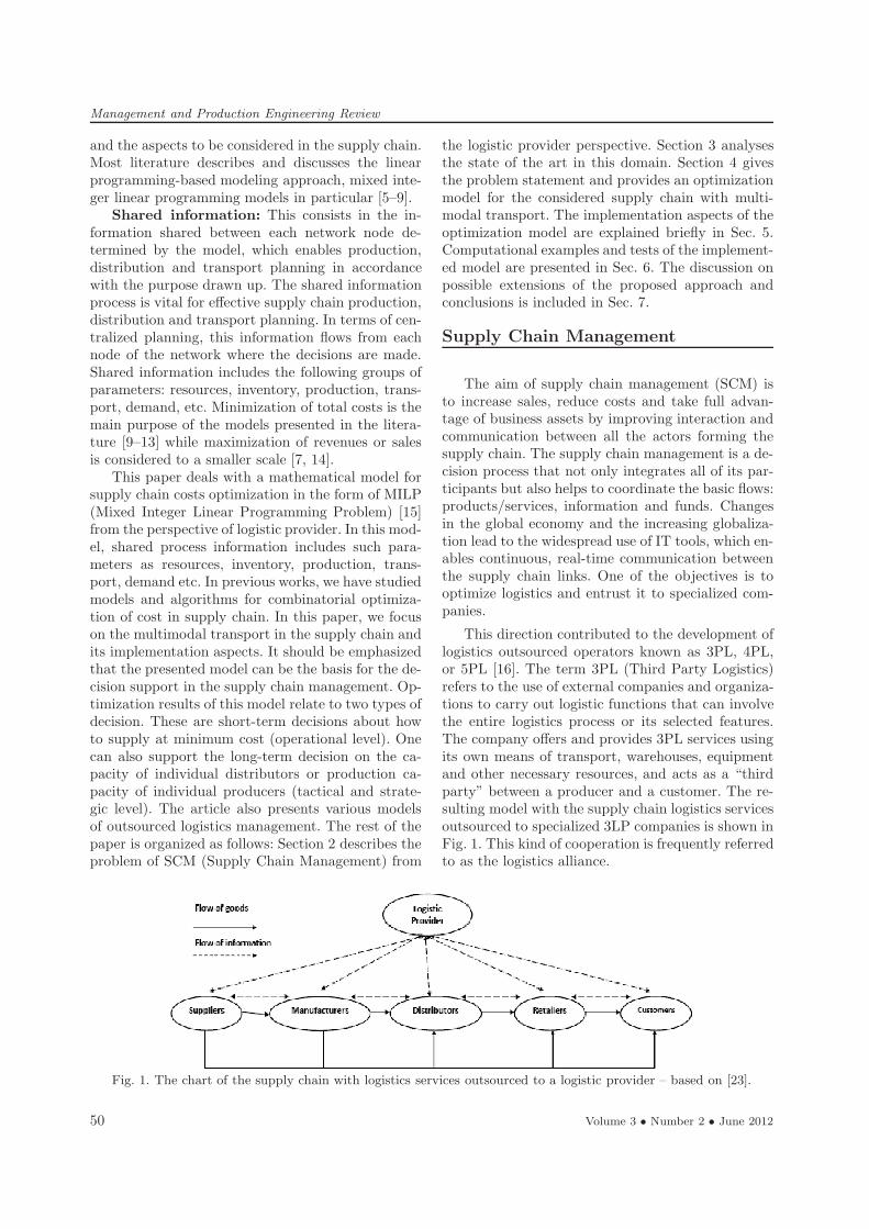
This direction contributed to the development oflogistics outsourced operators known as 3PL, 4PL,or 5PL [16]. The term 3PL (Third Party Logistics)refers to the use of external companies and organiza-tions to carry out logistic functions that can involvethe entire logistics process or its selected features.The company offers and provides 3PL services usingits own means of transport, warehouses, equipmentand other necessary resources, and acts as a “thirdparty” between a producer and a customer. The re-sulting model with the supply chain logistics servicesoutsourced to specialized 3LP companies is shown inFig. 1. This kind of cooperation is frequently referredto as the logistics alliance.

Fig. 1. The chart of the supply chain with logistics services outsourced to a logistic provider – based on [23].

50 Volume 3 • Number 2 • June 2012


4PL (Fourth-Party Logistics) is a certain evolu-tion of the 3PL concept to provide greater flexibilityand adaptation to the needs of the client. 4PL com-panies and organizations operate primarily by man-aging the information flow within the entire supplychain. Unlike the 3PL, responsible for only a selectedsegment, a 4PL coordinates logistics processes alongthe whole length of the chain (from raw materials toend-buyers). The 4PL model enables the 3PL oper-ator to become a coordinator and integrator of theflows, not just an operator of physical displacementof goods. Very often, its subcontractors are 3PL oreven 2PL (Second Party Logistics) operators, i.e.,transport companies and warehouses. The companythat uses the services of a 4PL provider is in contactwith only one operator who manages and integratesall types of resources and oversees the entire func-tionality across the supply chain. 4PL providers, hav-ing a complete picture of the supply chain and largeIT capabilities may offer optimization and decisionsupport advisory services [17]. Further developmentof logistics outsourcing resulted in the creation of5LP model (Fifth Party Logistics) – providers of in-tegrated logistics services that can design and imple-ment flexible and networked supply chains to caterto the needs of all participants (manufacturers, sup-pliers, carriers and end users).

State of art and motivation

Simultaneously considering the supply chain pro-duction, distribution processes in distribution cen-ters and transport-planning problems greatly ad-vances the efficiency of all processes. The literaturein the field is vast, so an extensive review of existingresearch on the topic is extremely helpful in mod-

eling and research. Comprehensive surveys on theseproblems and their generalizations were published,for example in [3].In our approach, we are considering a case of the

supply chain where:

• The shared information process in the supplychain consists of resources (capacity, versatili-ty, costs), inventory (capacity, versatility, costs,time), production (capacity, versatility, costs),product (volume), transport (cost, mode, time),demand, etc.(Fig. 2, Fig. 3).

• The transport is multimodal. (Several modes oftransport.A limited number of means of transportfor each mode).

• Different products are combined in one batch oftransport.

• The cost of supplies is presented in the form ofa function (in this approach linear function of fixedand variable costs).

• Different decision levels are considered simultane-ously.

Decision levels in supply chains are mainly classi-fied by the extent or effect of the decision to be madein terms of time. For instance, at the strategic level,the decisions made in relation to selecting produc-tion, storage and distribution locations, etc shouldbe identified. At the tactical level however, the as-pects such as production and distribution planning,assigning production and transport capacities, inven-tories and managing safety inventories are identified.Finally, at the operational level, replenishment anddelivery operations are classified [3]. Most of the re-viewed works focus on the tactical decision level [6–8,10–12, 18, 19]. Only few works deal with the prob-lems taken together for the different decision levels[5, 13].

Fig. 2. The part of the supply chain network with marked indices of individual participants (elements). Dashed linemarks one of the possible routes of delivery.

Volume 3 • Number 2 • June 2012 51


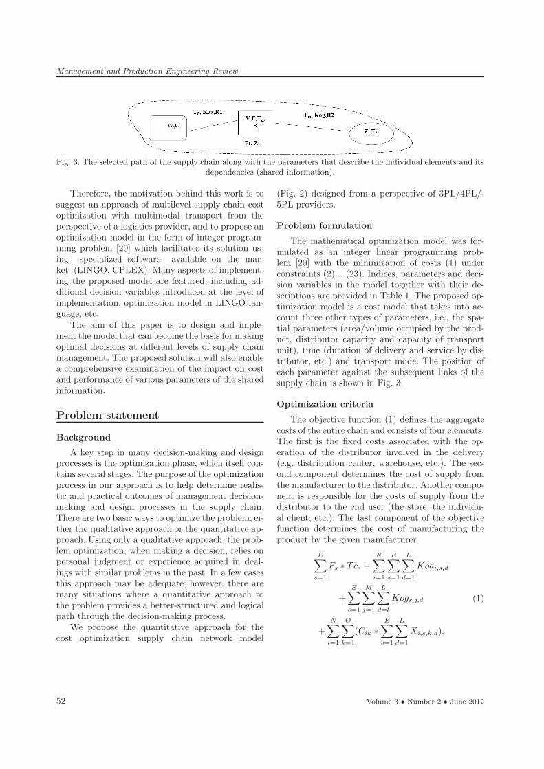
Fig. 3. The selected path of the supply chain along with the parameters that describe the individual elements and itsdependencies (shared information).

Therefore, the motivation behind this work is tosuggest an approach of multilevel supply chain costoptimization with multimodal transport from theperspective of a logistics provider, and to propose anoptimization model in the form of integer program-ming problem [20] which facilitates its solution us-ing specialized software available on the mar-ket (LINGO, CPLEX). Many aspects of implement-ing the proposed model are featured, including ad-ditional decision variables introduced at the level ofimplementation, optimization model in LINGO lan-guage, etc.The aim of this paper is to design and imple-

ment the model that can become the basis for makingoptimal decisions at different levels of supply chainmanagement. The proposed solution will also enablea comprehensive examination of the impact on costand performance of various parameters of the sharedinformation.

Problem statement

Background

A key step in many decision-making and designprocesses is the optimization phase, which itself con-tains several stages. The purpose of the optimizationprocess in our approach is to help determine realis-tic and practical outcomes of management decision-making and design processes in the supply chain.There are two basic ways to optimize the problem, ei-ther the qualitative approach or the quantitative ap-proach. Using only a qualitative approach, the prob-lem optimization, when making a decision, relies onpersonal judgment or experience acquired in deal-ings with similar problems in the past. In a few casesthis approach may be adequate; however, there aremany situations where a quantitative approach tothe problem provides a better-structured and logicalpath through the decision-making process.We propose the quantitative approach for the

cost optimization supply chain network model

(Fig. 2) designed from a perspective of 3PL/4PL/-5PL providers.

Problem formulation

The mathematical optimization model was for-mulated as an integer linear programming prob-lem [20] with the minimization of costs (1) underconstraints (2) .. (23). Indices, parameters and deci-sion variables in the model together with their de-scriptions are provided in Table 1. The proposed op-timization model is a cost model that takes into ac-count three other types of parameters, i.e., the spa-tial parameters (area/volume occupied by the prod-uct, distributor capacity and capacity of transportunit), time (duration of delivery and service by dis-tributor, etc.) and transport mode. The position ofeach parameter against the subsequent links of thesupply chain is shown in Fig. 3.

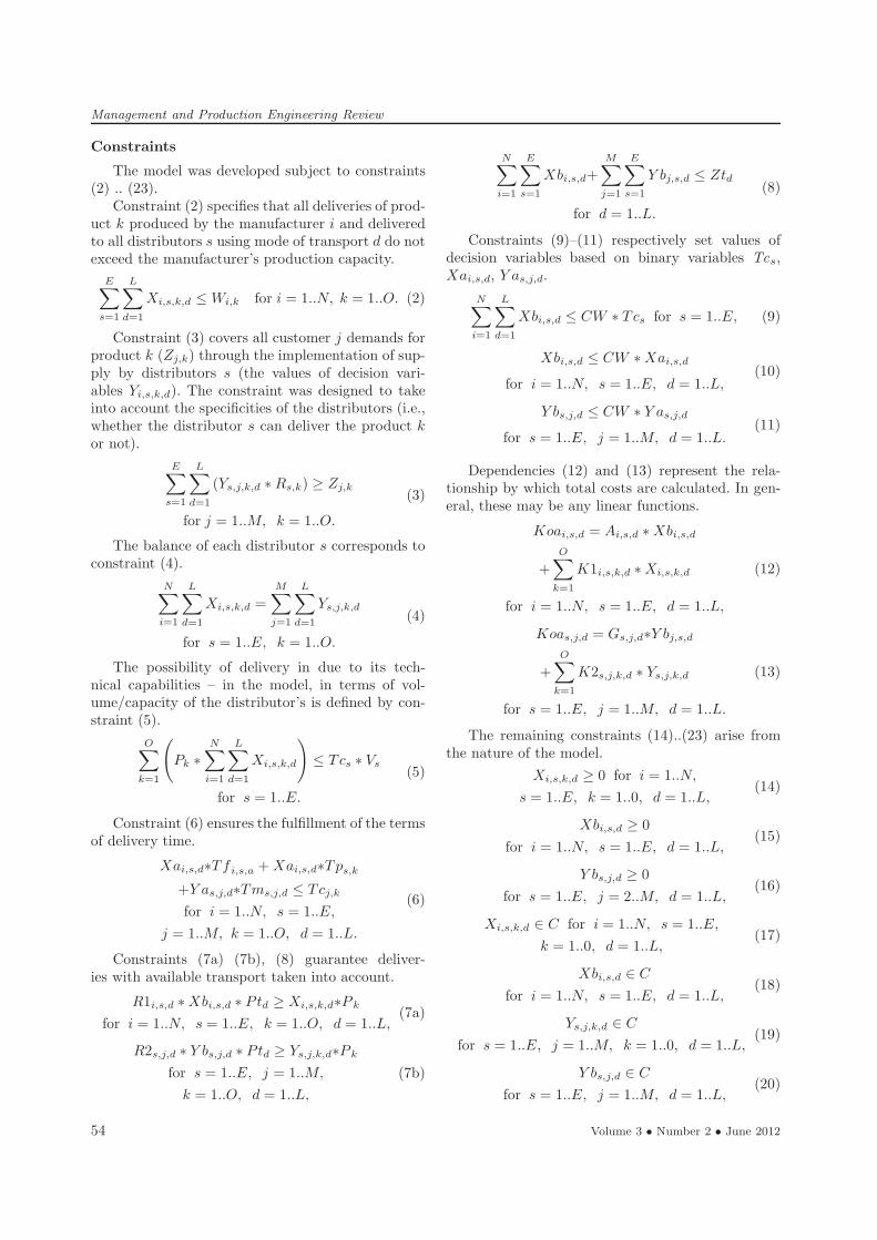
Optimization criteria

The objective function (1) defines the aggregatecosts of the entire chain and consists of four elements.The first is the fixed costs associated with the op-eration of the distributor involved in the delivery(e.g. distribution center, warehouse, etc.). The sec-ond component determines the cost of supply fromthe manufacturer to the distributor. Another compo-nent is responsible for the costs of supply from thedistributor to the end user (the store, the individu-al client, etc.). The last component of the objectivefunction determines the cost of manufacturing theproduct by the given manufacturer.

E∑

s=1

Fs ∗ Tcs +

N∑

i=1

E∑

s=1

L∑

d=1

Koai,s,d

+

E∑

s=1

M∑

j=1

L∑

d=l

Kogs,j,d

+

N∑

i=1

O∑

k=1

(Cik ∗

E∑

s=1

L∑

d=1

Xi,s,k,d).

(1)



Table 1

Summary indices, parameters and decision variables of the mathematical optimization model.

Symbol Description

Indices

k product type (k = 1..0)

j delivery point/customer/city (j = 1..M)

i manufacturer/factory (i = 1..N)

s distributor /distribution center (s = 1..E)

d mode of transport (d = 1..L)

N number of manufacturers/factories

M number of delivery points/customers

E number of distributors

O number of product types

L number of mode of transport

Input parameters

Fs the fixed cost of distributor/distribution center s (s = 1..E)

Pk the area/volume occupied by product k (k = 1..O)

Vs distributor s maximum capacity/volume (s = 1..E)

Wik factory production capacity for product k (i = 1..N) (k = 1..O)

Cik the cost of product k at factory i (i = 1..N) (k = 1..O)

Rsk if distributor s (s = 1.E) can deliver product k (k = 1..O) then Rsk = 1, otherwise Rsk = 0

Tpsk the time needed for distributor s (s = 1..E) to prepare the shipment of product k (k = 1..O)

Tcjk the cut-off time of delivery to the delivery point/customer j (j = 1..M) of product k (k = 1..O)

Zjk customer demand/order j (j = 1..M) for product k (k = 1..O)

Ztd the number of transport units using mode of transport d (d = 1..L)

Ptd the capacity of transport unit using mode of transport d (d = 1..L)

Tfisd the time of delivery from manufacturer i to distributor s using mode of transport d (i = 1..N) (s = 1..E)(d = 1..L)

K1iskd the variable cost of delivery of product k from manufacturer i to distributor s using mode of transport d

d (d = 1..L) (i = 1..N) (s = 1..E) (k = 1..O)

R1isd if manufacturer i can deliver to distributor s using mode of transport d then R1isd = 1, otherwise R1isd = 0

(d = 1..L) (s = 1..E) (i = 1..N)

Aisd the fixed cost of delivery from manufacturer i to distributor s using mode of transport d (d = 1..L) (i = 1..N)(s = 1..E)

Koasjd the total cost of delivery from distributor s to customer j using mode of transport d (d = 1..L) (s = 1..E)(j = 1..M)

Tmsjd the time of delivery from distributor s to customer j using mode of transport d (d = 1..L) (s = 1..E) (j = 1..M)

K2sjkd the variable cost of delivery of product k from distributor s to customer j using mode of transport d d (d = 1..L)(s = 1..E) (k = 1..O) (j = 1..M)

R2sjd if distributor s can deliver to customer j using mode of transport d then R2sjd = 1, otherwise R2sjd = 0

(d = 1..L) (s = 1..E) (j = 1..M)

Gsjd the fixed cost of delivery from distributor s to customer j using mode of transport d (s = 1..E) (j = 1..M)(k = 1..O)

Kogsjd the total cost of delivery from distributor s to customer j using mode of transport d (d = 1..L) (s = 1..E)(j = 1..M) (k = 1..O)

Decision variables

Xiskd delivery quantity of product k from manufacturer i to distributor s using mode of transport d

Xaisd if delivery is from manufacturer i to distributor s using mode of transport d then Xaisd = 1, otherwiseXaisd = 0

Xbisd the number of courses from manufacturer i to distributor s using mode of transport d

Ysjkd delivery quantity of product k from distributor s to customer j using mode of transport d

Y asjd if delivery is from distributor s to customer j using mode of transport d then Y asjd = 1, otherwise Y asjd = 0

Y bsjd the number of courses from distributor s to customer j using mode of transport d

Tcs If distributor s participates in deliveries, then Tcs = 1, otherwise Tcs = 0

CW Arbitrarily large constant



Constraints

The model was developed subject to constraints(2) .. (23).Constraint (2) specifies that all deliveries of prod-

uct k produced by the manufacturer i and deliveredto all distributors s using mode of transport d do notexceed the manufacturer’s production capacity.

E∑

s=1

L∑

d=1

Xi,s,k,d ≤ Wi,k for i = 1..N, k = 1..O. (2)

Constraint (3) covers all customer j demands forproduct k (Zj,k) through the implementation of sup-ply by distributors s (the values of decision vari-ables Yi,s,k,d). The constraint was designed to takeinto account the specificities of the distributors (i.e.,whether the distributor s can deliver the product k

or not).

E∑

s=1

L∑

d=1

(Ys,j,k,d ∗ Rs,k) ≥ Zj,k

for j = 1..M, k = 1..O.

(3)

The balance of each distributor s corresponds toconstraint (4).

N∑

i=1

L∑

d=1

Xi,s,k,d =

M∑

j=1

L∑

d=1

Ys,j,k,d

for s = 1..E, k = 1..O.

(4)

The possibility of delivery in due to its tech-nical capabilities – in the model, in terms of vol-ume/capacity of the distributor’s is defined by con-straint (5).

O∑

k=1

(

Pk ∗N∑

i=1

L∑

d=1

Xi,s,k,d

)

≤ Tcs ∗ Vs

for s = 1..E.

(5)

Constraint (6) ensures the fulfillment of the termsof delivery time.

Xai,s,d∗Tf i,s,a + Xai,s,d∗Tps,k

+Y as,j,d∗Tms,j,d ≤ Tcj,k

for i = 1..N, s = 1..E,

j = 1..M, k = 1..O, d = 1..L.

(6)

Constraints (7a) (7b), (8) guarantee deliver-ies with available transport taken into account.

R1i,s,d ∗ Xbi,s,d ∗ Ptd ≥ Xi,s,k,d∗P k

for i = 1..N, s = 1..E, k = 1..O, d = 1..L,(7a)

R2s,j,d ∗ Y bs,j,d ∗ Ptd ≥ Ys,j,k,d∗P k

for s = 1..E, j = 1..M,

k = 1..O, d = 1..L,

(7b)

N∑

i=1

E∑

s=1

Xbi,s,d+

M∑

j=1

E∑

s=1

Y bj,s,d ≤ Ztd

for d = 1..L.

(8)

Constraints (9)–(11) respectively set values ofdecision variables based on binary variables Tcs,Xai,s,d, Y as,j,d.

N∑

i=1

L∑

d=1

Xbi,s,d ≤ CW ∗ Tcs for s = 1..E, (9)

Xbi,s,d ≤ CW ∗ Xai,s,d

for i = 1..N, s = 1..E, d = 1..L,(10)

Y bs,j,d ≤ CW ∗ Y as,j,d

for s = 1..E, j = 1..M, d = 1..L.(11)

Dependencies (12) and (13) represent the rela-tionship by which total costs are calculated. In gen-eral, these may be any linear functions.

Koai,s,d = Ai,s,d ∗ Xbi,s,d

+

O∑

k=1

K1i,s,k,d ∗ Xi,s,k,d

for i = 1..N, s = 1..E, d = 1..L,

(12)

Koas,j,d = Gs,j,d∗Y bj,s,d

+

O∑

k=1

K2s,j,k,d ∗ Ys,j,k,d

for s = 1..E, j = 1..M, d = 1..L.

(13)

The remaining constraints (14)..(23) arise fromthe nature of the model.

Xi,s,k,d ≥ 0 for i = 1..N,

s = 1..E, k = 1..0, d = 1..L,(14)

Xbi,s,d ≥ 0

for i = 1..N, s = 1..E, d = 1..L,(15)

Y bs,j,d ≥ 0

for s = 1..E, j = 2..M, d = 1..L,(16)

Xi,s,k,d ∈ C for i = 1..N, s = 1..E,

k = 1..0, d = 1..L,(17)

Xbi,s,d ∈ C

for i = 1..N, s = 1..E, d = 1..L,(18)

Ys,j,k,d ∈ C

for s = 1..E, j = 1..M, k = 1..0, d = 1..L,(19)

Y bs,j,d ∈ C

for s = 1..E, j = 1..M, d = 1..L,(20)



Xai,s,d ∈ {0, 1}

for i = 1..N, s = 1..E, d = 1..L,(21)

Y as,j,d ∈ {0, 1}

for s = 1..E, j = 2..M, d = 1..L,(22)

Tcs ∈ {0, 1} for s = 1..E. (23)

Method developed

The model was implemented in “LINGO” byLINDO Systems [21]. “LINGO” Optimization Mod-eling Software is a powerful tool for building andsolving mathematical optimization models. “LIN-GO” package provides the language to build opti-mization models and the editor program includingall the necessary features and built-in “solvers” in asingle integrated environment. “LINGO” is designedto model and solve linear, nonlinear, quadratic, in-teger and stochastic optimization problems. Modelimplementation is possible in two basic ways. Thefirst way is to enter the model into the “LINGO”editor in the explicit form, that is, a full functionof the objective with all the constraints, parameters,etc. Although this is an intuitive approach and con-sistent with the standard form of linear program-ming [20], it is not very useful in practice. This isdue to the size of models implemented in practice.For the small example presented in chapter Compu-tational examples, the number of decision variablesand constraints was 592 and 1125, respectively. Theother way is to use the “LINGO” language of math-ematical modeling, an integral part of the “LINGO”package, whose basic syntax elements are shown inTable 1. For the real examples with sizes exceedingseveral decision variables, the construction and im-plementation of the model is only possible using themodeling language (Table 2, Fig. 7). The basic ele-ments of mathematical modeling language syntax of“LINGO” are presented in Table 1.

Table 2The basic syntax of “LINGO” mathematical modeling

language

Mathematical nomenclature LINGO syntax

Minimum MIN =PZjkt @sum(ORDER (j, k, t))

j = 1..M for each customer @FOR(CUSTOMERS (j))

(j) in the set of customers

• *

= =

X ∈integer @gin(X)

X ∈ {0, 1} @bin(X)

Load input parameters p p=@file(dane.ldt)

from the file dane.ldt

The model can be saved in a text file using anytext editor and with a standard extension *. lng and*. ldt data file. The structure of the model is com-posed of sections. The main section is the MODELsection, which begins with the word MODEL: andends with the word END. Other sections may beintegrated in this section. The most important sec-tions, highlighted by the relevant keywords are: sec-tion SETS (SET: ENDSETS) and DATE (DATE:enddate). In the SETS section one can define typesof simple or complex objects, and their mutual rela-tionships. In the implemented model, simple objectsare exemplified by types such as products, factories,etc.; complex objects: production, distribution, etc.In this section, the parameters and variables of themodel are assigned to particular types. DATA sectionallows initiating or assigning values to individual pa-rameters of the model. There are two methods to doit in the “LINGO” package. Either place the numer-ical data directly in the section or make referencesto the place where those data files are included. Thismethod of model construction ensures the separationof data from the relevant model, which is very impor-tant because the change in data values or even theirsize does not require any changes in the objectivefunction or constraints. Only the model implement-ed in the implicit form has such a feature.

Computational examples

The cost optimization model (1)..(23) was im-plemented in the “LINGO” environment. Figure 7shows the implicit model. Optimization was per-formed for three examples: P1, P2 and P3.

Fig. 4. Transport network of multi-modal optimal solu-tion (Fc

opt= 74810) for P1. The number of hauls is 16.

All cases relate to the supply chain with two man-ufacturers (i = 1..2), three distributors (s = 1.3),



four recipients (j = 1..4), four mode of transport(d = 1..4) and five types of products (k = 1..5).The examples differ in capacity available to the dis-tributors (Vs) and number of transport units usingmode of transport d(Ztd). The numeric data for allthe model parameters from Table 1 are presented inAppendix A (Table 3)





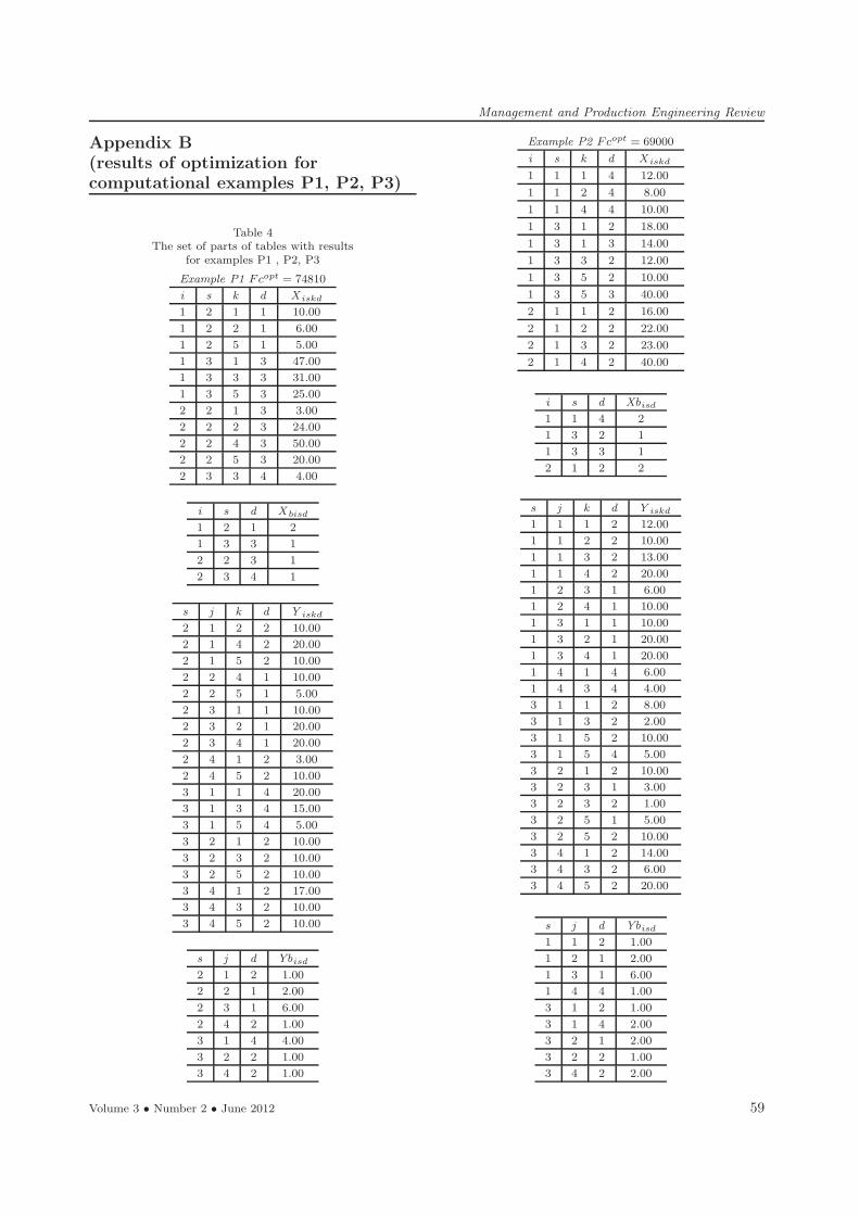
Optimization started after the implementation ofthe model in the LINGOmathematical modeling lan-guage (Fig. 7). Optimization results are shown inAppendix B (Table 4) and Fig. 8 (only for P1) withthe parameters of the process of searching for theoptimal solution: the number of iterations, the op-timization algorithm used (Branch-and-Bound) [20],the number of decision variables in the integer con-straints, etc. The optimization process involves find-ing the global solution for the specific data Appen-dix A (Table 3), which in this case means the lowestcost of satisfying customer needs through the sup-ply chain and amounts to Fcopt = 74810 for P1,Fcopt = 69000 for P2 and Fcopt = 75420 for P3.Transportation networks diagrams showing the num-

ber of hauls (no number means one) correspondingto the optimal solutions for P1, P2, P3 are shownsequentially in Figs. 4–6.

Fig. 7. Part of the file scm.lng (the supply chain costoptimization model in LINGO).



At the same time, the specific values of decisionvariables that minimize the cost are determined (Ta-ble 4). These values represent, among other things,the volume of supplies from the manufacturer tothe distributor of selected products using mode oftransport (Xi,s,k,d) and the supply of products fromspecific distributors to selected customers/recipients(Ys,j,k,d). Based on these variables, one can make adecision at the current operating level.The values of decision variables Yb,s,j,d, Xb,i,s,d

determine the number of courses using transportmode. Based on these variables one can make a deci-sion from the tactical level, which includes the modeof transport and the need for different means oftransport.Another way to use the implemented model is to

determine the effect of the change in the model pa-rameters on the cost. One can analyze in detail thesensitivity of solutions depending on the parametersKo, A, G, C, T, V, Zt etc. The article focused onthe effect of parameter V and Zt.Numerous analyses of that kind can be conduct-

ed. For further studies and especially long-term de-cision support, the optimization model was extend-ed at the implementation stage. Auxiliary variableswere introduced at implementation stage Vx s (thevalue corresponds to the distributor’s uptake capaci-ty) and Wx i,k (production capacity utilization ratesfor manufacturer i of product k). The analysis of thedecision variables values Vx s andWx ik Appendix B(Table 5) has an impact on strategic decision mak-ing level of production capacity or dealer locationand capacity.

Fig. 8. LINGO results window, for P1.

Conclusions

The paper presents a model of optimizing sup-ply chain costs. Creating the model in the form ofa MILP problem undoubtedly facilitates its solutionusing mathematical programming tools available in“LINGO” package [21] or “CPLEX” [22] and oth-ers. Of course, the model should be implementedin one, selected environment package. Implementa-tion of the model in the “LINGO” package and thecomputational experiments were presented. The ap-proach from the perspective of an optimizing logisticsprovider that has access to all data and all partici-pants in the downstream chain is very interesting.

After the implementation of the language fromthe mathematical modeling package “LINGO”,a number of computational experiments were con-ducted. Three of them in the form of examples P1,P2and P3 were described in the article. Based on theexperimental results, analysis and previous experi-ence, the authors can state that the proposed modeland its implementation ensure a very large range ofapplications. First, they allow finding the distribu-tion flows (decision variables) for the modeled sup-ply chain, which minimize the global cost satisfyingthe needs of customers. Second, they offer numer-ous possibilities for decision support in supply chainmanagement through the solutions sensitivity analy-sis, determination of the range and quality of theimpact of various parameters on the cost and evenon the structure of the supply chain. The analysispresented in the article, only in terms of the capacityavailable to distributors and the number of transportunits fully confirms this statement.

Appendix A(data for computationalexamples P1, P2, P3)

Table 3

The set of parts of data tables for examples P1,P2 and P3.

s Fs V s-P1,P2 V s -P3

1 10 000 2 000 2 000

2 15 000 2 500 2 500

3 12 000 1 500 1 200

d Ptd Ztd -P1,P3 Ztd -P2

1 50 10 10

2 200 4 8

3 800 2 1

4 60 5 5



j k Z jk Tcjk j k Z jk Tcjk

1 1 20 10 2 1 10 10

1 2 10 10 2 2 0 10

1 3 15 10 2 3 10 10

1 4 20 10 2 4 10 10

1 5 15 20 2 5 15 20

3 1 10 10 4 1 20 10

3 2 20 10 4 2 0 10

3 3 0 10 4 3 10 10

3 4 20 10 4 4 0 10

3 5 0 20 4 5 20 20

i k C ik W ik i k C ik W ik

1 1 100 100 2 1 150 100

1 2 200 100 2 2 210 100

1 3 200 100 2 3 150 100

1 4 300 100 2 4 250 100

1 5 300 100 2 5 350 100

s k Rsk Tpsk s k Rsk Tpsk

1 1 1 2 2 1 1 1

1 2 1 2 2 2 1 1

1 3 1 2 2 3 0 1

1 4 1 2 2 4 1 1

1 5 0 2 2 5 1 1

3 1 1 3Tmsjd=

1, Tf isd=13 2 1 3

3 3 1 3

3 4 0 3

3 5 1 3

i s d Aisd R1 isd k Pk

1 1 1 2 1 1 10

1 1 2 1 1 2 15

1 1 3 1 1 3 15

1 1 4 2 1 4 10

1 2 1 2 1 5 20

1 2 2 1 1

1 2 3 1 1

1 2 4 2 0

1 3 1 2 1

1 3 2 1 1

1 3 3 1 1

1 3 4 2 0

2 1 1 2 1

2 1 2 1 1

2 1 3 1 1

2 1 4 2 0

2 2 1 2 1

2 2 2 1 1

2 2 3 1 1

2 2 4 2 0

2 1 1 2 1

2 1 2 1 0

2 1 3 1 0

2 1 4 2 1

s j d Gisd R2 isd

1 1 1 1 1

1 1 2 1 1

1 1 3 1 0

1 1 4 1 1

1 2 1 1 1

1 2 2 1 1

1 2 3 1 1

1 2 4 1 0

1 3 1 1 1

1 3 2 1 1

1 3 3 1 1

1 3 4 1 0

1 4 1 1 1

1 4 2 1 1

1 4 3 1 1

1 4 4 1 1

2 1 1 1 1

2 1 2 1 1

2 1 3 1 0

2 1 4 1 1

2 2 1 1 1

2 2 2 1 1

2 2 3 1 1

2 2 4 1 0

2 3 1 1 1

2 3 2 1 1

2 3 3 1 1

2 3 4 1 0

2 4 1 1 1

2 4 2 1 1

2 4 3 1 1

2 4 4 1 1

3 1 1 1 1

3 1 2 1 1

3 1 3 1 0

3 1 4 1 1

3 2 1 1 1

3 2 2 1 1

3 2 3 1 1

3 2 4 1 0

3 3 1 1 1

3 3 2 1 1

3 3 3 1 1

3 3 4 1 0

3 4 1 1 1

3 4 2 1 1

3 4 3 1 1

3 4 4 1 1



Appendix B(results of optimization forcomputational examples P1, P2, P3)

Table 4The set of parts of tables with results

for examples P1 , P2, P3

Example P1 Fcopt = 74810

i s k d X iskd

1 2 1 1 10.00

1 2 2 1 6.00

1 2 5 1 5.00

1 3 1 3 47.00

1 3 3 3 31.00

1 3 5 3 25.00

2 2 1 3 3.00

2 2 2 3 24.00

2 2 4 3 50.00

2 2 5 3 20.00

2 3 3 4 4.00

i s d X bisd

1 2 1 2

1 3 3 1

2 2 3 1

2 3 4 1

s j k d Y iskd

2 1 2 2 10.00

2 1 4 2 20.00

2 1 5 2 10.00

2 2 4 1 10.00

2 2 5 1 5.00

2 3 1 1 10.00

2 3 2 1 20.00

2 3 4 1 20.00

2 4 1 2 3.00

2 4 5 2 10.00

3 1 1 4 20.00

3 1 3 4 15.00

3 1 5 4 5.00

3 2 1 2 10.00

3 2 3 2 10.00

3 2 5 2 10.00

3 4 1 2 17.00

3 4 3 2 10.00

3 4 5 2 10.00

s j d Ybisd

2 1 2 1.00

2 2 1 2.00

2 3 1 6.00

2 4 2 1.00

3 1 4 4.00

3 2 2 1.00

3 4 2 1.00


i s k d X iskd

1 1 1 4 12.00

1 1 2 4 8.00

1 1 4 4 10.00

1 3 1 2 18.00

1 3 1 3 14.00

1 3 3 2 12.00

1 3 5 2 10.00

1 3 5 3 40.00

2 1 1 2 16.00

2 1 2 2 22.00

2 1 3 2 23.00

2 1 4 2 40.00

i s d Xbisd

1 1 4 2

1 3 2 1

1 3 3 1

2 1 2 2

s j k d Y iskd

1 1 1 2 12.00

1 1 2 2 10.00

1 1 3 2 13.00

1 1 4 2 20.00

1 2 3 1 6.00

1 2 4 1 10.00

1 3 1 1 10.00

1 3 2 1 20.00

1 3 4 1 20.00

1 4 1 4 6.00

1 4 3 4 4.00

3 1 1 2 8.00

3 1 3 2 2.00

3 1 5 2 10.00

3 1 5 4 5.00

3 2 1 2 10.00

3 2 3 1 3.00

3 2 3 2 1.00

3 2 5 1 5.00

3 2 5 2 10.00

3 4 1 2 14.00

3 4 3 2 6.00

3 4 5 2 20.00

s j d Ybisd

1 1 2 1.00

1 2 1 2.00

1 3 1 6.00

1 4 4 1.00

3 1 2 1.00

3 1 4 2.00

3 2 1 2.00

3 2 2 1.00

3 4 2 2.00




i s k d X iskd

1 2 1 3 60.00

1 2 2 3 30.00

1 2 4 3 40.00

1 2 5 3 18.00

1 3 3 3 31.00

1 3 5 3 32.00

2 2 4 1 10.00

2 3 3 4 4.00

i s d Xbisd

1 2 3 1

1 3 3 1

2 2 1 2

2 3 4 1

s j k d Y iskd

2 1 1 2 20.00

2 1 1 2 20.00

2 1 2 2 10.00

2 1 4 2 20.00

2 1 5 2 3.000

2 2 1 1 10.00

2 2 4 1 10.00

2 2 5 1 5.000

2 3 1 1 10.00

2 3 2 1 20.00

2 3 4 1 20.00

2 4 1 2 20.00

2 4 5 2 10.00

3 1 3 4 15.00

3 1 5 4 12.00

3 2 3 2 10.00

3 2 5 2 10.00

3 4 3 2 10.00

3 4 5 2 10.00

s j d Ybisd

2 1 2 1.00

2 2 1 2.00

2 3 1 6.00

2 4 2 1.00

3 1 4 4.00

3 2 2 1.00

3 4 2 1.00

Table 5The set of parts of tables with results for examples P1, P2,

P3 – decision variables Wxs,k, Vxs.

P1 P2 P3

s k Wxsk s k Wxsk s k Wxsk

1 1 57 1 1 44 1 1 69

1 2 6 1 2 8 1 2 30

1 3 31 1 3 12 1 3 31

1 5 30 1 4 10 1 4 40

2 1 3 1 5 50 1 5 50

2 2 24 2 1 16 2 3 4

2 3 4 2 2 22 2 4 10

2 4 50 2 3 23

2 5 20 2 4 40

P1 P2 P3

s Vxs s Vxs s Vxs

2 1580 1 1575 2 1910

3 1495 3 1500 3 1165

References

[1] Simchi-Levi D., Kaminsky P., Simchi-Levi E., De-signing and Managing the Supply Chain: Concepts,Strategies, and Case Studies, McGraw-Hill, ISBN978-0-07-119896-7, New York 2003.

[2] Shapiro J.F., Modeling the Supply Chain, ISBN 978-0-534-37741, Duxbury Press, 2001.

[3] Huang G.Q., Lau J.S.K., Mak K.L., The impactsof sharing production information on supply chaindynamics: a review of the literature, Internation-al Journal of Production Research, 41, 1483–1517,2003.

[4] Beamon B.M., Chen V.C.P., Performance analysisof conjoined supply chains, International Journal ofProduction Research, 39, 3195–3218, 2001.

[5] Kanyalkar A.P., Adil G.K., An integrated aggregateand detailed planning in a multi-site production en-vironment using linear programming, Internation-al Journal of Production Research, 43, 4431–4454,2005.

[6] Perea-lopez E., Ydstie B.E., Grossmann I.E.,A model predictive control strategy for supply chainoptimization, Computers and Chemical Engineer-ing, 27, 1201–1218, 2003.

[7] Park Y.B., An integrated approach for productionand distribution planning in supply chain manage-ment, International Journal of Production Research,43, 1205–1224, 2005.

[8] Jung H., Jeong B., Lee C.G., An order quanti-ty negotiation model for distributor-driven supplychains, International Journal of Production Eco-nomics, 111, 147–158, 2008.

[9] Rizk N., Martel A., D’amours S.,Multi-item dynam-ic production-distribution planning in process indus-tries with divergent finishing stages, Computers andOperations Research, 33, 3600–3623, 2006.

[10] Selim H., Am C., Ozkarahan I., Collaborativeproduction-distribution planning in supply chain:a fuzzy goal programming approach, TransportationResearch Part E-Logistics and Transportation Re-view, 44, 396–419, 2008.

[11] Lee Y.H., Kim S.H., Optimal production–distribution planning in supply chain managementusing a hybrid simulation-analytic approach, Pro-ceedings of the 2000 Winter Simulation Conference,1 and 2, 1252–1259, 2000.



[12] Chern C.C., Hsieh J.S., A heuristic algorithm formaster planning that satisfies multiple objectives.Computers and Operations Research, 34, 3491–3513, 2007.

[13] Jang Y.J., Jang S.Y., Chang B.M., Park J., Acombined model of network design and produc-tion/distribution planning for a supply network,Computers and Industrial Engineering, 43, 263–281,2002.

[14] Timpe C.H., Kallrath J., Optimal planning in largemulti-site production networks, European Journal ofOperational Research, 126, 422–435, 2000.

[15] Schrijver A., Theory of Linear and Integer Pro-gramming, ISBN 0-471-98232-6, John Wiley & Sons,1998.

[16] Ho H., Lim C., The logistics players – From 1PL to5PL, Morgan Stanley: China Logistics, 8–9, 2001.

[17] Jianming Yao, Decision optimization analysis onsupply chain resource integration in fourth party lo-

gistics, Journal of Manufacturing Systems, 29, 121–129, 2010.

[18] Chern C.C., Hsieh J.S., A heuristic algorithm formaster planning that satisfies multiple objectives,Computers and Operations Research, 34, 3491–3513, 2007.

[19] Torabi S.A., Hassini E., An interactive possibilis-tic programming approach for multiple objective sup-ply chain master planning, Fuzzy Sets and Systems,159, 193–214, 2008.

[20] Schrijver A., Theory of Linear and Integer Pro-gramming, ISBN 0-471-98232-6, John Wiley & Sons,1998.

[21] www.lindo.com.

[22] www.ibm.com.

[23] Hokey Min, Gengui Zhou, Supply chain modeling:past, present and future, Computers and IndustrialEngineering, 43, 231-249, 2002.


mathematicalprogrammingmodel ofcostoptimizationforsupplychain...

Documents