Mathematical Statistics

Stockholm University

Smoothing splines

in non-life insurance pricing

Viktor Grgic

Examensarbete 2008:3

Postal address:Mathematical StatisticsDept. of MathematicsStockholm UniversitySE-106 91 StockholmSweden

Internet:http://www.math.su.se/matstat

Mathematical StatisticsStockholm UniversityExamensarbete 2008:3,http://www.math.su.se/matstat

Smoothing splines in non-life insurance pricing

Viktor Grgic∗

March 2008

Abstract

In non-life insurance, almost every rating analysis involves one orseveral continuous variables. Traditionally, the approach has beento divide the possible values of the variable into intervals whereaftergeneralized linear models (GLM) are employed for estimation; an al-ternative way of dealing with continuous variables is via polynomialregression. The object of this thesis is to explore the possible use ofcubic smoothing splines represented in B-spline form for modellingthe effect of continuous variables. We will investigate the cases of oneto several rating variables as well as interaction between a continu-ous and a categorical variable. The cross validation (CV) approach isused to select the optimal value of the smoothing parameter. Our im-plementation of smoothing splines has been carried out in SAS/IMLand applied to a variety of pricing problems, using in particular motorinsurance data from Lansforsakringar insurance group.

∗E-mail: viktor.grgic@lansforsakringar.se. Supervisors: Bjorn Johansson and Ola Hoss-jer.

Acknowledgements

This work constitutes a 30-credit Master’s thesis in mathematicalstatistics at Stockholm University and has been carried out at Lans-forsakringar insurance group.

I am deeply indebted first and foremost to my supervisor at Lansfor-sakringar, Dr. Bjorn Johansson. Unconditionally he shared his enthu-siasm, expert knowledge and time throughout all stages of this thesis.I also wish to extend my sincere thanks and appreciation to the rest ofthe staff at Actuarial Department (Forsakringsekonomi) at Lansfor-sakringar for providing me with all the actuarial and administrativesupport and advice.

I would also like to thank my second supervisor, Prof. Ola Hossjerof Stockholm University for his valuable suggestions and thoroughperusal of the final draft. Lastly, I wish to acknowledge the Directorof Studies at the Department of Mathematical Statistics at StockholmUniversity, Dr. Mikael Andersson, for his help with finding this thesis.

2

Contents

1 Introduction 4

2 Non-life insurance pricing with GLM 8

3 Smoothing splines 10

3.1 Cubic splines . . . . . . . . . . . . . . . . . . . . . . . . . . . 10

3.2 B-splines . . . . . . . . . . . . . . . . . . . . . . . . . . . . . . 13

3.3 One rating variable . . . . . . . . . . . . . . . . . . . . . . . . 16

3.4 Automatic selection of the smoothing parameter . . . . . . . . 23

3.5 Several rating variables . . . . . . . . . . . . . . . . . . . . . . 25

3.6 Interaction between a continuous and a categorical variable . . 28

4 Case studies 31

4.1 Moped . . . . . . . . . . . . . . . . . . . . . . . . . . . . . . . 32

4.2 Lorry . . . . . . . . . . . . . . . . . . . . . . . . . . . . . . . . 34

4.3 Car . . . . . . . . . . . . . . . . . . . . . . . . . . . . . . . . . 44

5 Conclusions 49

6 References 51

3

1 Introduction

The price of a car or home insurance policy depends on a number of factors,

such as age of the policyholder, the annual mileage or the floor area of a

house. Initially this was motivated by the concept of fairness : the price of

a policy should stand in proportion to the expected cost of claims of the

policyholder. For instance, in household insurance it would be unreasonable

to charge the same premium for a large estate as for a small house. Nowadays,

another main driving force is competition: an insurance company with an

inferior rating structure will lose profit. This is due to the fact that overrated,

i.e. profitable, costumers will tend to choose another insurance company,

whereas underrated (non-profitable) customers will accumulate, thus causing

a deterioration of the business. This mechanism has lead to an ever increasing

number of rating variables and elaborate methods for making the best use of

them.

The use of statistical models in the pricing of non-life insurance products

has a long tradition. For many years methods developed for these special

purposes by insurance mathematicians, actuaries, were used. However, dur-

ing recent years, many insurance companies have started to use generalized

linear models (GLM) for the purpose of finding a good rating structure. The

starting point seems to be the paper by Brockman and Wright (1992). Apart

from the fact that the models are reasonable, there is a great advantage of us-

ing well-understood methods and commercial software. The basic reference

is still the book by McCullagh and Nelder (1989).

Almost every rating analysis involves one or several continuous variables,

such as age of the policyholder or weight of the vehicle. Traditionally, the

approach has been to divide the possible values of the variable into intervals

and treat it as if it was a categorical variable. This procedure, in the sequel

referred to as interval subdivision method, has several disadvantages. To

begin with, one gets a rating structure where the premium takes sudden

jumps — for instance there may be a substantial difference in the premiums

between two customers that are 29 and 30 years old, but not if they were 28

4

and 29 years old, all depending on how the subdivision into intervals is made.

Secondly, the method seems unsatisfactory from a statistical point of view:

for values close to a subdivision point, observations pertaining to close values

in the adjoining interval have no influence at all, whereas observations for

values at the other end of the interval do, although the latter should be much

less relevant. Furthermore, information is lost when grouping the values of

the explanatory variable into intervals, not making efficient use of the data.

Finally, the process of finding a good subdivision into intervals is tedious and

time consuming.

An alternative way of dealing with continuous variables is via polynomial

regression, but this method has several weaknesses as well. For instance, the

polynomial’s value at a certain point can be heavily influenced by observa-

tions far from the point. Also, in pursuit of a better fit we may increase the

degree of the polynomial, but this can lead to uncontrolled oscillation of the

curve, especially at the end points, where we commonly have sparse data.

Finally, the fit can only be increased in discrete steps and the shape of the

curve can change drastically when the degree of the polynomial is increased

one step. These objections aside, polynomial regression works well in many

situations.

As an example of polynomial regression we consider the LIDAR data in Rup-

pert et al. (2003), shown in Figure 1.1. LIDAR stands for Light Detection

and Ranging and serves a similar purpose as RADAR. Clearly, the mean

response as a function of the explanatory variable appears to be far from

linear. Assuming a normal error structure (which is questionable due to the

obvious non-constant variance, but let us leave that aside), we have fitted

polynomials of degree 2-10 to the LIDAR data. The results are shown in

Figure 1.2. One notices the sometimes drastic change of the curve when the

degree of the polynomial is increased, as well as a certain wiggliness, espe-

cially at the edges. We will return to this example later, as a first illustration

of the method which is the subject in this thesis. For a thorough discussion

of these data, see Ruppert et al. (2003).

The problem of curve fitting without making specific assumptions concerning

5

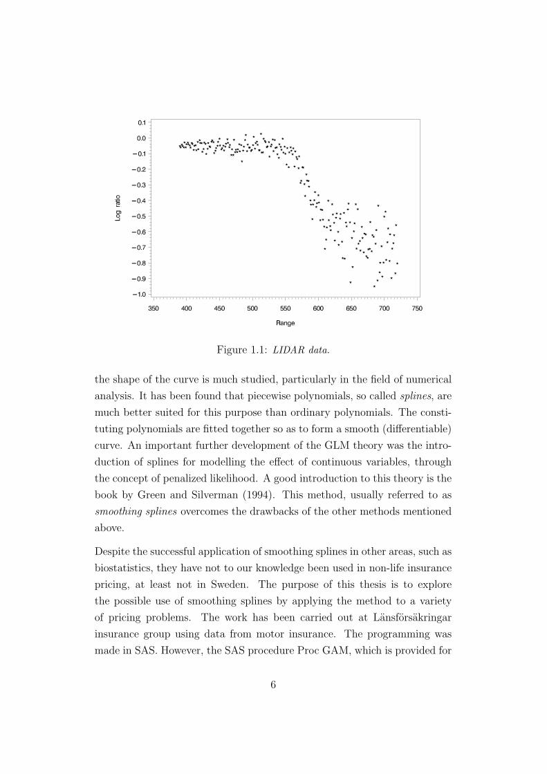
Figure 1.1: LIDAR data.

the shape of the curve is much studied, particularly in the field of numerical

analysis. It has been found that piecewise polynomials, so called splines, are

much better suited for this purpose than ordinary polynomials. The consti-

tuting polynomials are fitted together so as to form a smooth (differentiable)

curve. An important further development of the GLM theory was the intro-

duction of splines for modelling the effect of continuous variables, through

the concept of penalized likelihood. A good introduction to this theory is the

book by Green and Silverman (1994). This method, usually referred to as

smoothing splines overcomes the drawbacks of the other methods mentioned

above.

Despite the successful application of smoothing splines in other areas, such as

biostatistics, they have not to our knowledge been used in non-life insurance

pricing, at least not in Sweden. The purpose of this thesis is to explore

the possible use of smoothing splines by applying the method to a variety

of pricing problems. The work has been carried out at Lansforsakringar

insurance group using data from motor insurance. The programming was

made in SAS. However, the SAS procedure Proc GAM, which is provided for

6

Figure 1.2: Higher degree polynomial fits to the LIDAR data.

fitting smoothing splines, has some severe limitations, in particular the lack

of a weight statement. Therefore, the actual data fitting was carried out in

SAS/IML, making use of its numerical procedures.

An outline of the thesis is as follows. Section 2 provides some basic facts

about pricing in non-life insurance using generalized linear models. In section

3 the basic theory of smoothing splines is summarized, focusing on the parts

most relevant for non-life insurance pricing. Section 4 contains three case

studies, each illustrating different aspects of the theory. The findings are

presented in a number of diagrams. Finally, some concluding remarks are

made in section 5.

7

2 Non-life insurance pricing with GLM

Insurance companies store large amounts of information concerning policies

and claims. These are gathered into databases which are the primary sources

for the rating analyses carried out by the actuaries.

The volume of an insurance portfolio or a group of policyholders are measured

in policy years. A rating analysis is based on data from a certain period, for

instance five years, and a policy valid during x days of this period counts as

x/365 policy years. The claim frequency of a group during some time period

is defined as the number of claims divided by the number of policy years.

Another important figure is the claim severity, the total cost of the claims

for a group divided by the number of claims. The total claim cost divided

by the number of policy years is called the risk premium. Obviously, the

risk premium is the product of the claim frequency and the claim severity.

One way of stating the fairness principle is that the expected risk premium

is what a policyholder should pay for a one year policy, excluding expenses.

Traditionally, a rating analysis has focused directly on the risk premium

and its dependence upon various rating variables, such as age and sex of

the policyholder. The paper by Brockman and Wright (1992) advocates the

separation of the analysis into claim frequency and claim severity. We shall

refer to the response variables claim frequency, severity and risk premium

under the common name key ratios.

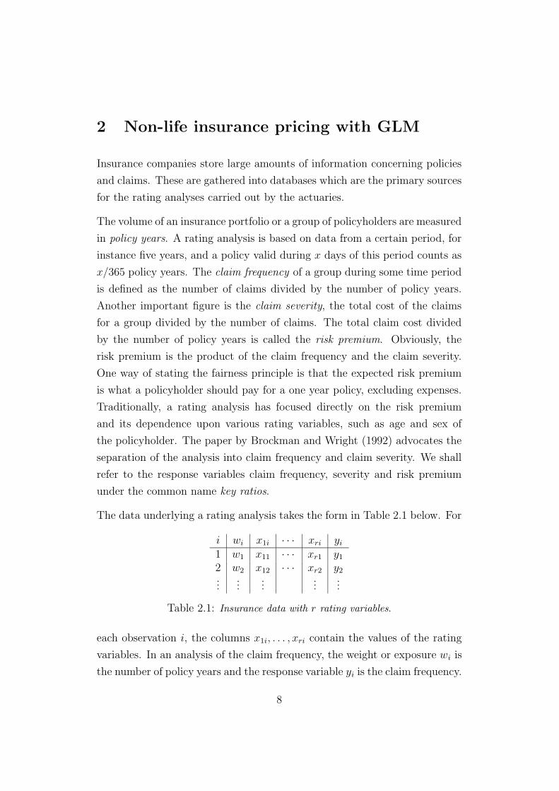
The data underlying a rating analysis takes the form in Table 2.1 below. For

i wi x1i · · · xri yi

1 w1 x11 · · · xr1 y1

2 w2 x12 · · · xr2 y2...

......

......

Table 2.1: Insurance data with r rating variables.

each observation i, the columns x1i, . . . , xri contain the values of the rating

variables. In an analysis of the claim frequency, the weight or exposure wi is

the number of policy years and the response variable yi is the claim frequency.

8

When analyzing the claim severity, wi is the number of claims and yi is the

claim severity.

Brockman and Wright (1992) also suggested using GLM for analyzing the

claim frequency and claim severity. If each yi in Table 2.1 is the outcome of

a random variable Yi, in a GLM it is assumed that the frequency function of

Yi may be written as

fYi(yi; θi, φ) = exp

yiθi − b(θi)

φ/wi

+ c(yi, φ, wi)

where θi is called the canonical parameter and φ the dispersion parameter.

This family of distributions is called exponential dispersion models. For in-

stance, the normal, Poisson and gamma distributions belong to this family.

One can show that

µi := E(Yi) = b′(θi)

σ2i := Var(Yi) = φ v(µi)/wi

where v(µi) = b′′(b′−1(µi)). It can be proved that the variance function

v(µ) uniquely characterizes the distribution within the family of exponential

dispersion models. In a claim frequency analysis, it is usually assumed that

the Yi has a Poisson distribution, which corresponds to v(µ) = µ. When

analyzing the claim severity, it is common to use a gamma distribution,

corresponding to v(µ) = µ2. Based on the concept of quasi likelihood it can be

argued that the important assumption is the dependency of the variance on

the mean and not the particular distributional form. The Poisson assumption

in the claim frequency case is seldomly questioned, and several studies show

that a quadratic variance function is usually appropriate for modelling the

claim severity.

A basic feature of GLM’s is that the variance of Yi depends on the explanatory

variables x1i, . . . , xri only through the mean µi. Another basic assumption,

motivating the name generalized linear models, is that the mean depends on

the explanatory variables through a relationship of the form

ηi = g(µi) =∑

j1

β1j1Φ1j1(x1i) + . . . +∑

jr

βrjrΦrjr

(xri) (2.1)

9

If the link function g is the identity function, we have a linear model. In

non-life insurance pricing, both for the claim frequency and claim severity,

one almost always assumes that the effect of the explanatory variables is

multiplicative, which corresponds to g(µ) = log µ. Again, studies prove

this to be a good model in both cases, and it is also the one traditionally

used for the risk premium by all Swedish insurance companies. If xpi is a

categorical variable, the function Φpj(xpi) takes the values 0 and 1 only. In

the polynomial regression case, we use Φpj(xpi) = xjpi.

For proofs of the statements made above and additional information on GLM

and its application to non-life insurance pricing, we refer to Ohlsson and

Johansson (2008).

3 Smoothing splines

A spline is, simply put, a function that consists of piecewise low degree

polynomials that are smoothly joined together at a number of fixed points.

So what exactly do we mean by smoothly? A cubic spline, for instance, is

constructed from cubic polynomials in such a way that the spline’s first and

second derivatives are continuous at each point. Although there are splines

of any order, for our purpose, it will be sufficient and necessary to work with

cubic splines. Sufficiency is partly motivated by the fact that our eyes are

not capable of perceiving third and higher order discontinuities; see Hastie

and Tibshirani (1990, pp. 22–23). In addition, cubic splines turn out to have

a certain optimality property when we start our discussion on their use in

statistical applications, which is the subject matter of this thesis.

3.1 Cubic splines

We start by deriving some essential results about cubic splines regarding

their existence and uniqueness. First, assume that we are given a set of m

ordered and distinct points t1, . . . , tm called knots. Furthermore, on each

10

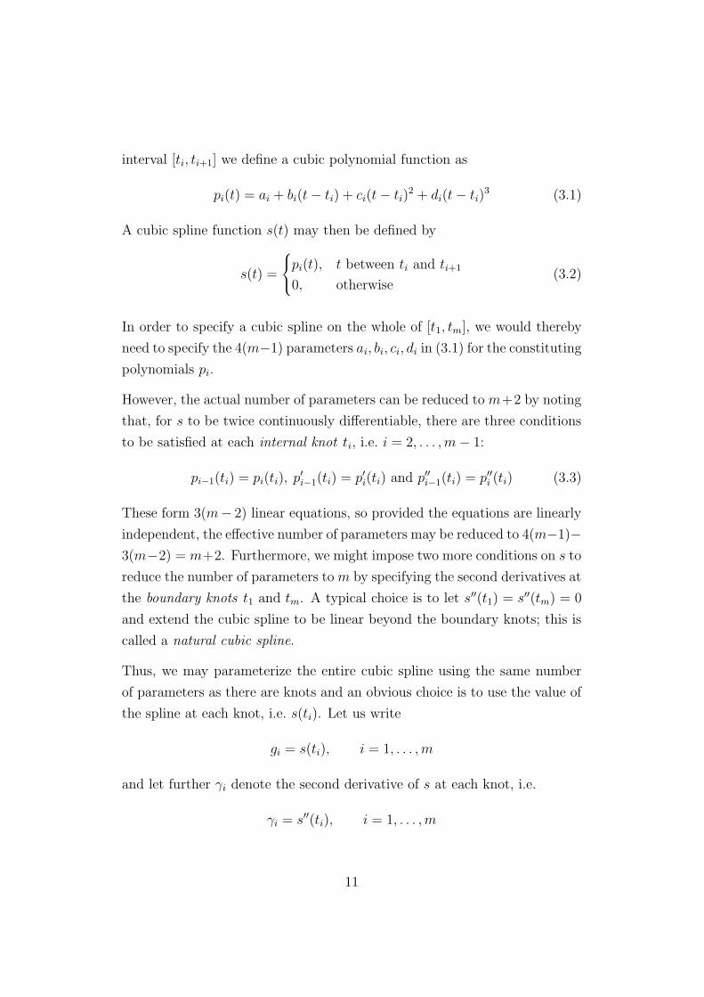
interval [ti, ti+1] we define a cubic polynomial function as

pi(t) = ai + bi(t − ti) + ci(t − ti)2 + di(t − ti)

3 (3.1)

A cubic spline function s(t) may then be defined by

s(t) =

pi(t), t between ti and ti+1

0, otherwise(3.2)

In order to specify a cubic spline on the whole of [t1, tm], we would thereby

need to specify the 4(m−1) parameters ai, bi, ci, di in (3.1) for the constituting

polynomials pi.

However, the actual number of parameters can be reduced to m+2 by noting

that, for s to be twice continuously differentiable, there are three conditions

to be satisfied at each internal knot ti, i.e. i = 2, . . . ,m − 1:

pi−1(ti) = pi(ti), p′i−1(ti) = p′i(ti) and p′′i−1(ti) = p′′i (ti) (3.3)

These form 3(m− 2) linear equations, so provided the equations are linearly

independent, the effective number of parameters may be reduced to 4(m−1)−

3(m−2) = m+2. Furthermore, we might impose two more conditions on s to

reduce the number of parameters to m by specifying the second derivatives at

the boundary knots t1 and tm. A typical choice is to let s′′(t1) = s′′(tm) = 0

and extend the cubic spline to be linear beyond the boundary knots; this is

called a natural cubic spline.

Thus, we may parameterize the entire cubic spline using the same number

of parameters as there are knots and an obvious choice is to use the value of

the spline at each knot, i.e. s(ti). Let us write

gi = s(ti), i = 1, . . . ,m

and let further γi denote the second derivative of s at each knot, i.e.

γi = s′′(ti), i = 1, . . . ,m

11

Finally, let hi denote the distance between knots, hi = ti+1 − ti. The condi-

tions in (3.3) give rise to a linear system of m− 2 equations to be solved for

the m − 2 unknowns γ2, . . . , γm−1, which may be written as

Aγ = r (3.4)

where

A =

13(h1 + h2) 1

6h2

16h2

13(h2 + h3) 1

6h3

16h3

13(h3 + h4) 1

6h4

. . .. . .

. . .16hm−3

13(hm−3 + hm−2) 1

6hm−2

16hm−2

13(hm−2 + hm−1)

and γ and r are column vectors with elements γ2, . . . , γm−1 and

r1 =g3 − g2

h2

−g2 − g1

h1

−1

6h1γ1

ri =gi+2 − gi+1

hi+1

−gi+1 − gi

hi

, i = 2, . . . ,m − 3

rm−2 =gm − gm−1

hm−1

−gm−1 − gm−2

hm−2

−1

6hm−1γm,

respectively.

The symmetric, tridiagonal (m − 2) × (m − 2) matrix A can be shown to

be strictly diagonally dominant (the main diagonal element is strictly larger

than the sum of the non-diagonal elements in each row/column) which implies

that the system (3.4) always has a unique solution. This solution can then be

used to determine the unknown coefficients ai, bi, ci, di of all the polynomials

in (3.2). Thereby we are ready to state two propositions that will be crucial

in the following; for details see Ohlsson and Johansson (2008).

Proposition 1. Let t1, . . . , tm be given points such that t1 < · · · < tm and

let g1, . . . , gm, γ1, γm be any real numbers. Then there exists a unique cubic

spline s(t) with knots t1, . . . , tm satisfying s(ti) = gi for i = 1, . . . ,m and

s′′(t1) = γ1, s′′(tm) = γm.

Proposition 2. A cubic spline s with knots t1, . . . , tm is uniquely determined

by the values s(t1), . . . , s(tm), s′′(t1), s′′(tm).

12

Observe here that Proposition 1 describes the typical setting when dealing

with interpolation problems, i.e. when we wish to fit a smooth and stable

curve through a set of points (ti, gi), i = 1, . . . ,m. The solution to this

numerical problem is called an interpolating spline.

The invention of splines and the first development of their theory are usually

credited to the Romanian-American mathematician Isaac Jacob Schoenberg

with his research paper from 1946. His choice of the term spline for the func-

tions that he was studying was due to the resemblance with the draftman’s

spline — a long, thin and flexible strip of wood or other material, initially

used by ship-builders to design the smooth curvatures of the ship’s hull.

Even though Schoenberg’s splines had all the benefits on their side contra

other methods, it took years before they were seriously used in practice due

to the heavy calculations involved. It was first with the advent of computers

that splines became widely used in the industrial world. Today, splines are an

essential tool to architects and engineers and are used extensively in many

different fields such as construction of railway lines, aircraft, ship and car

industries, 3D Graphics Rendering etc.

3.2 B-splines

In practice, splines are rarely implemented with the representation (3.2) due

to ill-conditioning. In this subsection we will introduce a superior and well-

conditioned representation where a spline will be expressed as a linear com-

bination of a set of basis functions called B-splines. The whole idea behind

this builds upon the fact that the set of splines with fixed knots t1, . . . , tm

forms a linear space, and as such usually has some sort of simple base.

The B-splines were originally defined using the concept of divided differences ;

see Curry and Schoenberg (1947). Here instead, we will use a recursive

approach and to begin with, let us define the base for the zeroth order splines

13

by

B0,i(t) =

1, t ∈ [ti, ti+1)

0, otherwise, i = 1, . . . ,m − 2

B0,i(t) =

1, t ∈ [ti, ti+1]

0, otherwise, i = m − 1

(3.5)

The higher order B-splines are then constructed from the following recursion

formulae

Bk+1,1(t) =t2 − t

t2 − t1Bk,1(t)

Bk+1,i(t) =t − tmax(i−k−1,1)

tmin(i,m) − tmax(i−k−1,1)

Bk,i−1(t) +tmin(i+1,m) − t

tmin(i+1,m) − tmax(i−k,1)

Bk,i(t),

i = 2, . . . ,m + k − 1

Bk+1,m+k(t) =t − tmax(m−1,1)

tm − tm−1

Bk,m+k−1(t)

(3.6)

For instance in the cubic spline case, i.e. when k = 2 above, we get the

following m + 2 basis functions expressed recursively in terms of B2,i

B3,1(t) =t2 − t

t2 − t1B2,1(t)

B3,2(t) =t − t1t2 − t1

B2,1(t) +t3 − t

t3 − t1B2,2(t)

B3,3(t) =t − t1t3 − t1

B2,2(t) +t4 − t

t4 − t1B2,3(t)

B3,i(t) =t − ti−3

ti − ti−3

B2,i−1(t) +ti+1 − t

ti+1 − ti−2

B2,i(t),

i = 4, . . . ,m − 1

B3,m(t) =t − tm−3

tm − tm−3

B2,m−1(t) +tm − t

tm − tm−2

B2,m(t)

B3,m+1(t) =t − tm−2

tm − tm−2

B2,m(t) +tm − t

tm − tm−1

B2,m+1(t)

B3,m+2(t) =t − tm−1

tm − tm−1

B2,m+1(t)

(3.7)

Notice here that the dimension of the space that the cubic B-splines form,

m + 2, agrees with the number of parameters that completely determines a

14

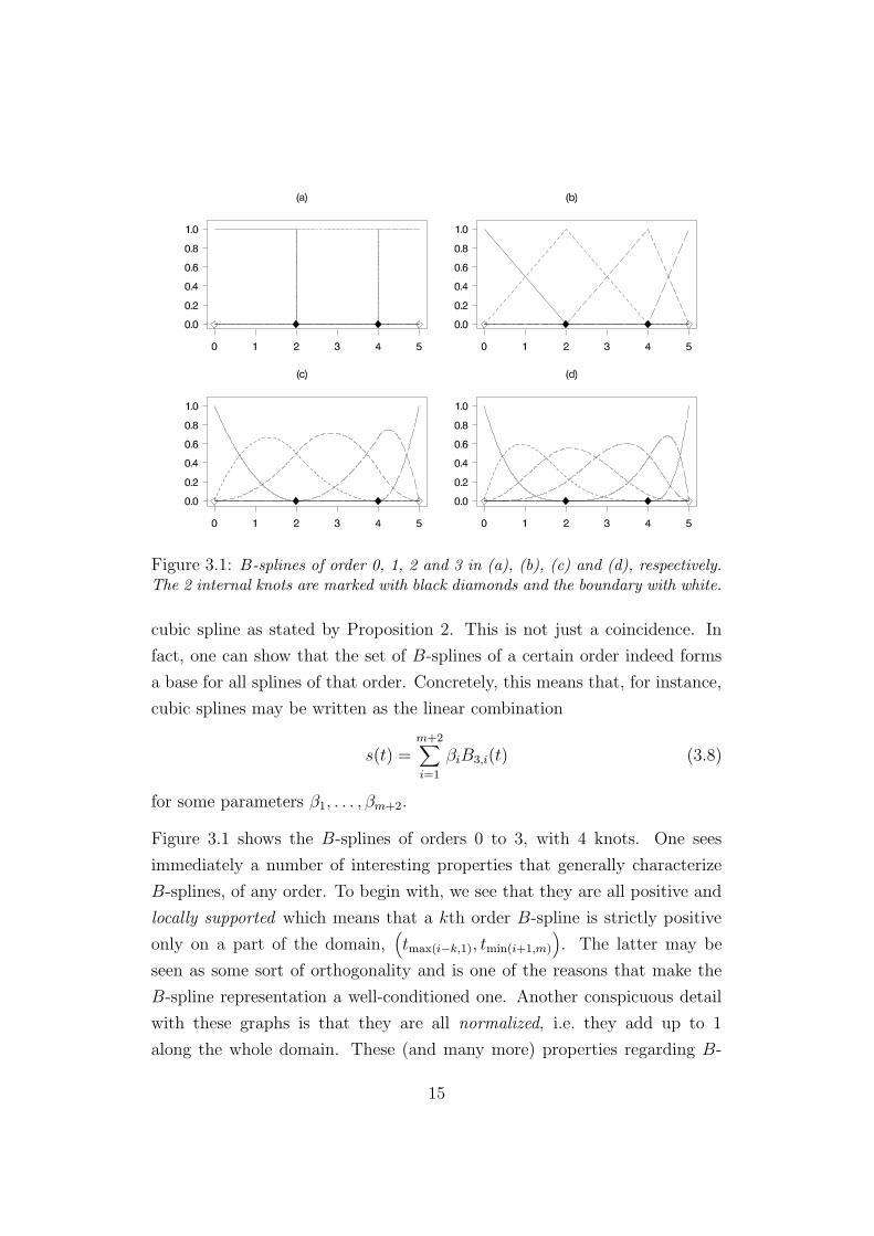
Figure 3.1: B-splines of order 0, 1, 2 and 3 in (a), (b), (c) and (d), respectively.The 2 internal knots are marked with black diamonds and the boundary with white.

cubic spline as stated by Proposition 2. This is not just a coincidence. In

fact, one can show that the set of B-splines of a certain order indeed forms

a base for all splines of that order. Concretely, this means that, for instance,

cubic splines may be written as the linear combination

s(t) =m+2∑

i=1

βiB3,i(t) (3.8)

for some parameters β1, . . . , βm+2.

Figure 3.1 shows the B-splines of orders 0 to 3, with 4 knots. One sees

immediately a number of interesting properties that generally characterize

B-splines, of any order. To begin with, we see that they are all positive and

locally supported which means that a kth order B-spline is strictly positive

only on a part of the domain,(

tmax(i−k,1), tmin(i+1,m)

)

. The latter may be

seen as some sort of orthogonality and is one of the reasons that make the

B-spline representation a well-conditioned one. Another conspicuous detail

with these graphs is that they are all normalized, i.e. they add up to 1

along the whole domain. These (and many more) properties regarding B-

15

splines can all be derived from the above recurrence relations; see Ohlsson

and Johansson (2008).

As already pointed out, the main emphasis in this paper is on cubic splines,

and so from now on the subindex 3 in B3,i(t) will be suppressed and we will

write Bi(t) instead.

3.3 One rating variable

All the results that we have derived until now have been of a purely mathe-

matical nature but nevertheless important in our discussion on how to take

advantage of splines when modelling the effect of a continuous variable. As we

mentioned earlier in this section, natural cubic splines have certain qualities

that make them unique among all twice continuously differentiable functions.

To prepare for this result, suppose that we want to analyze some insurance

data as shown in Table 3.1.

i xi wi yi

1 x1 w1 y1

2 x2 w2 y2...

......

...

Table 3.1: Insurance data with a single continuous variable.

On each row i, we are given the value of a continuous variable xi, the weight

wi and the observation yi. Even though a variable is regarded as continuous,

for instance car owner’s age, in most cases the values that we observe are

discrete. For instance, age may be measured in years. Let z1 < · · · < zm

denote the possible values of the variable and let further Ik denote the set

of all i where xi = zk. We may now define the aggregated weights and

observations as

wk =∑

i∈Ik

wi, yk =1

wk

∑

i∈Ik

wiyi

Suppose now that we relax the strict parametric assumptions made in (2.1)

16

and only assume that we wish to model the dependence of µi on xi via

ηi = g(µi) = f(xi)

for some arbitrary smooth function f . This is the simplest example of the

rich family of models called generalized additive models (GAM), as set out

by Hastie and Tibshirani (1990).

Despite its limited practical importance when modelling insurance data, we

will start the analysis with the normal distribution case due to its simplicity

and later on extend it to the Poisson and gamma cases. The link function in

the normal case is the identity link, i.e. ηi = µi, and the log-likelihood func-

tion is `(yi, µi) = −12

(

log(2πφ) + wi(yi − µi)2/φ

)

. In a GLM the parameters

are typically estimated by maximizing the log-likelihood∑

i `(yi, µi). For the

purpose of estimating the means, we can achieve exactly the same thing by

minimizing the deviance D =∑

i 2[

`(yi, yi)−`(yi, µi)]

instead. In the normal

case we have

D =1

φ

∑

i

wi(yi − µi)2 (3.9)

where the dispersion parameter φ is usually estimated separately and may

be removed from the expression (3.9). With the notation introduced above

and using that µi = f(zk) when i ∈ Ik, it is easy to see that minimizing the

deviance (3.9) is equivalent to minimizing

D =m∑

k=1

wk(yk − f(zk))2 (3.10)

From this we see that there are in fact infinitely many functions that minimize

the deviance; any twice continuously differentiable function f that interpo-

lates the points (zk, yk), k = 1, . . . ,m would do the job. The idea now is to

modify (3.10) by adding a term that constrains how much the function may

oscillate or wiggle and to look for a function that minimizes the penalized

deviance

∆ =m∑

k=1

wk

(

yk − f(zk))2

+ λ∫ b

a

(

f ′′(t))2

dt (3.11)

where a ≤ z1 and b ≥ zm. The choice of the integrated squared second

derivative feels intuitive as a measure of the curvature in a C2-function, and it

17

approaches zero as the function flattens out. This integral is then multiplied

by a smoothing parameter λ to control the influence of this penalty term on

the function f(t).

We have earlier hinted that splines play a decisive role and one can now

show, with the aid of Proposition 1, that a unique minimizing function of

the penalized deviance in (3.11) exists and is a natural cubic spline with the

knots z1 < · · · < zm; for details see Ohlsson and Johansson (2008). The

function s(t) that minimizes ∆ will be called the cubic smoothing spline. It

is important here to notice that the minimizing s(t) is a unique minimizer

only for a fixed value of λ. In fact, we have a whole family of splines sλ(t)

that minimize ∆ as we vary the smoothing parameter along the positive real

line.

In the previous subsection, we saw that a cubic spline may be written as a

linear combination of B-splines of third order. By substituting f(t) with (3.8)

in the above expression for ∆, we obtain the following equation instead

∆(β1, . . . , βm+2) =m∑

k=1

wk

(

yk −m+2∑

j=1

βjBj(zk)

)2

+ λm+2∑

j=1

m+2∑

k=1

βjβkΩjk (3.12)

where Ωjk =∫ zm

z1B′′

j (t)B′′

k(t)dt; the details of the calculation of Ωjk’s are given

in Ohlsson and Johansson (2008). Our task now is to find the vector β =

(β1, . . . , βm+2)T that minimizes ∆(β1, . . . , βm+2) and by using the customary

method of equating the partial derivatives to zero, we get the following system

of equations

m∑

k=1

m+2∑

j=1

wkβjBj(zk)B`(zk) + λm+2∑

j=1

βjΩj` =m∑

k=1

wkykB`(zk),

` = 1, . . . ,m + 2

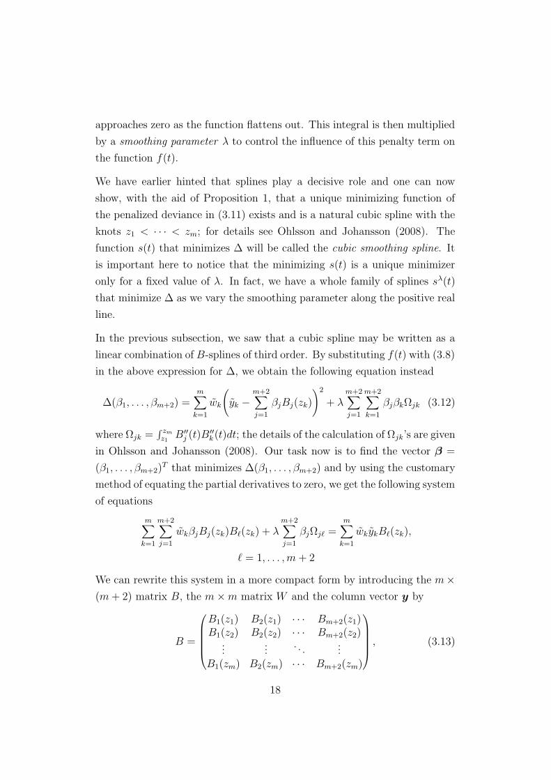
We can rewrite this system in a more compact form by introducing the m×

(m + 2) matrix B, the m × m matrix W and the column vector y by

B =

B1(z1) B2(z1) · · · Bm+2(z1)B1(z2) B2(z2) · · · Bm+2(z2)

......

. . ....

B1(zm) B2(zm) · · · Bm+2(zm)

, (3.13)

18

W = diag(w1, . . . , wm) (3.14)

and y = (y1, . . . , ym)T , respectively. Thus, we arrive at the penalized normal

equations(

BT WB + λΩ)

β = BT Wy (3.15)

where the difference from traditional normal equations is the term λΩ.

Depending on the number of knots, the constituting matrices may be quite

large, causing the computation of the inverse of BT WB + λΩ to become

expensive both performance- and memory-wise. However, due to the local

support property of B-spline functions, the symmetric and strictly positive-

definite matrices BT WB and Ω are 5- and 7-banded, respectively. This

allows us to perform the Cholesky decomposition on the consequently 7-

banded matrix BT WB +λΩ, which in addition to back substitution gives us

the solution to (3.15) in a very cost-effective way.

Later we will consider a method of choosing the best value of the smoothing

parameter with regard to a certain criterion. With this particular value of

λ, the smoothing spline fit to the LIDAR data is displayed in Figure 3.2.

Compared to Figure 1.2, this fit is far more pleasing in that it manages

to follow the trend of the data well, yet at the same time being smooth

and stable enough to completely eliminate the wiggles associated with the

polynomial regression.

The span of the smoothing spline fit to the LIDAR data is depicted in Fig-

ure 3.3 and we see the visual diversity one may achieve by tweaking the

smoothing parameter. One can also show that the degrees of freedom de-

crease as we increase λ.

When modelling claim frequency and severity, with a multiplicative structure

of the mean, i.e. ηi = log µi, the corresponding equations become nonlinear

and must be solved iteratively. To realize this, we start with the Poisson case

where the log-likelihood function is `(yi, µi) = wi

(

yi log µi−µi

)

+wiyi log wi−

log(wiyi)!. Using that µi = expf(zk) when i ∈ Ik, the deviance can now

19

Figure 3.2: Smoothing spline fit to the LIDAR data with automatic selection ofthe smoothing parameter.

be written as

D = 2m∑

k=1

wk

(

yk log yk − ykf(zk) − yk + expf(zk))

One can again show that there are infinitely many functions minimizing D.

However, using the same penalty technique as previously, one arrives at the

same conclusion that the minimizer must be a natural cubic spline. Thus,

our task is to find β that minimizes the penalized deviance

∆ = 2m∑

k=1

wk

yk log yk − yk

m+2∑

j=1

βjBj(zk) − yk + exp

m+2∑

j=1

βjBj(zk)

+ λm+2∑

j=1

m+2∑

k=1

βjβkΩjk

corresponding to the normal case’s (3.12). Setting the partial derivatives

20

Figure 3.3: Two extreme cases of smoothing spline fits to the LIDAR data: inter-polating natural cubic spline as λ → 0 (thin solid line) and linear regression lineas λ → ∞ (thick solid line).

∂∆/∂β` to zero gives us the following system of equations

−m∑

k=1

wkykB`(zk) +m∑

k=1

wkB`(zk) exp

m+2∑

j=1

βjBj(zk)

+ λm+2∑

j=1

βjΩj` = 0,

` = 1, . . . ,m + 2(3.16)

These equations are nonlinear in β and therefore cannot be directly expressed

on the same simplified form as in the normal case. Instead, we are forced to

determine the minimizing β by some iterative method.

Let f`(β1, . . . , βm+2) denote the left hand side of the `th equation in (3.16).

Applying the Newton-Raphson procedure,

f`(β[n]1 , . . . , β

[n]m+2) +

m+2∑

j=1

(

β[n+1]j − β

[n]j

)

∂

∂βj

f`(β[n]1 , . . . , β

[n]m+2) = 0,

` = 1, . . . ,m + 2

we obtain the following system of linear equations after some algebraic trans-

21

positions

m+2∑

j=1

m∑

k=1

wkγ[n]k Bj(zk)B`(zk)β

[n+1]j + λ

m+2∑

j=1

β[n+1]j Ωj`

=m∑

k=1

wkγ[n]k

yk/γ[n]k − 1 +

m+2∑

j=1

β[n]j Bj(zk)

B`(zk),

` = 1, . . . ,m + 2

where γ[n]k denotes the mean in the nth iteration

γ[n]k = exp

m+2∑

j=1

β[n]j Bj(zk)

Introducing the m × m diagonal matrix W [n] and the column vector y[n] by

(

W [n])

kk= wkγ

[n]k ,

(

y[n])

k= yk/γ

[n]k − 1 +

m+2∑

j=1

β[n]j Bj(zk) (3.17)

we can now, analogously with the normal case, rewrite the above linear sys-

tem on matrix form as

(

BT W [n]B + λΩ)

β[n+1] = BT W [n]y[n] (3.18)

Here, it is worth noting that, in each iteration, these are exactly the same

equations as (3.15) if we replace the weight matrix and observation vector

by those given in (3.17). This remark will be of importance in the discussion

on automatic selection of the smoothing parameter in the non-normal cases.

In the multiplicative gamma case, reasoning as in the Poisson case, we arrive

at a system of linear equations on the same matrix form (3.18), where the

weight matrix and observation vector are given by

(

W [n])

kk= wk

yk

γ[n]k

,(

y[n])

k= 1 −

γ[n]k

yk

+m+2∑

j=1

β[n]j Bj(zk) (3.19)

As an intuitive starting value for the iterations, we take the logarithm of the

mean observation

(

β[0])

j= log

∑mk=1 wkyk∑m

k=1 wk

, j = 1, . . . ,m + 2

22

The convergence of β is in most cases achieved rapidly and usually requires

3–5 iterations to reach the accuracy of 0.5 ·10−2. In the gamma case this may

be improved by using Fisher’s scoring method, which is basically the same

Newton-Raphson method with the exception of the Hessian being replaced

by its expected value. This means that in the expression of the weight matrix

in (3.19) we now have instead(

W [n])

kk= wk while y[n] is unchanged.

3.4 Automatic selection of the smoothing parameter

We will now present one commonly used method for data-based selection

of the smoothing parameter, called cross-validation (CV). To begin with,

we will explore the normal distribution case first and then extend it to the

Poisson and gamma cases.

Thus, assume that we are given a set of normally distributed data. Suppose

now that we remove an observation k and, for some fixed λ, find the minimiz-

ing spline sλ−k(t) for this diminished set. The essence of the cross-validation

technique lies in the fact that, if λ is well-selected, then sλ−k(zk) should be a

good predictor of the omitted observation yk. Proceeding in the same man-

ner with all the remaining m− 1 observations, the best λ is chosen to be the

value that minimizes the sum of squared prediction errors

CV (λ) =m∑

k=1

wk

(

yk − sλ−k(zk)

)2

(3.20)

Thus, to minimize CV (λ), it seems we would need m spline computations for

each λ, which involves a large number of calculations. However, it is shown

in Ohlsson and Johansson (2008) that, in the normal case, CV (λ) may be

expressed in terms of only a single spline computation for the full data set.

It turns out that (3.20) may instead be replaced by the following

CV (λ) =m∑

k=1

wk

(

yk − s(zk)

1 − Akk

)2

(3.21)

where s(zk) is the minimizing spline for the full data set evaluated at the

knots, and A = B(

BT WB + λΩ)

−1BT W .

23

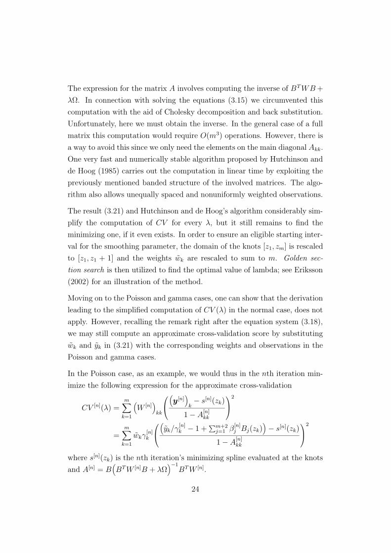
The expression for the matrix A involves computing the inverse of BT WB +

λΩ. In connection with solving the equations (3.15) we circumvented this

computation with the aid of Cholesky decomposition and back substitution.

Unfortunately, here we must obtain the inverse. In the general case of a full

matrix this computation would require O(m3) operations. However, there is

a way to avoid this since we only need the elements on the main diagonal Akk.

One very fast and numerically stable algorithm proposed by Hutchinson and

de Hoog (1985) carries out the computation in linear time by exploiting the

previously mentioned banded structure of the involved matrices. The algo-

rithm also allows unequally spaced and nonuniformly weighted observations.

The result (3.21) and Hutchinson and de Hoog’s algorithm considerably sim-

plify the computation of CV for every λ, but it still remains to find the

minimizing one, if it even exists. In order to ensure an eligible starting inter-

val for the smoothing parameter, the domain of the knots [z1, zm] is rescaled

to [z1, z1 + 1] and the weights wk are rescaled to sum to m. Golden sec-

tion search is then utilized to find the optimal value of lambda; see Eriksson

(2002) for an illustration of the method.

Moving on to the Poisson and gamma cases, one can show that the derivation

leading to the simplified computation of CV (λ) in the normal case, does not

apply. However, recalling the remark right after the equation system (3.18),

we may still compute an approximate cross-validation score by substituting

wk and yk in (3.21) with the corresponding weights and observations in the

Poisson and gamma cases.

In the Poisson case, as an example, we would thus in the nth iteration min-

imize the following expression for the approximate cross-validation

CV [n](λ) =m∑

k=1

(

W [n])

kk

(

y[n])

k− s[n](zk)

1 − A[n]kk

2

=m∑

k=1

wkγ[n]k

(

yk/γ[n]k − 1 +

∑m+2j=1 β

[n]j Bj(zk)

)

− s[n](zk)

1 − A[n]kk

2

where s[n](zk) is the nth iteration’s minimizing spline evaluated at the knots

and A[n] = B(

BT W [n]B + λΩ)

−1BT W [n].

24

3.5 Several rating variables

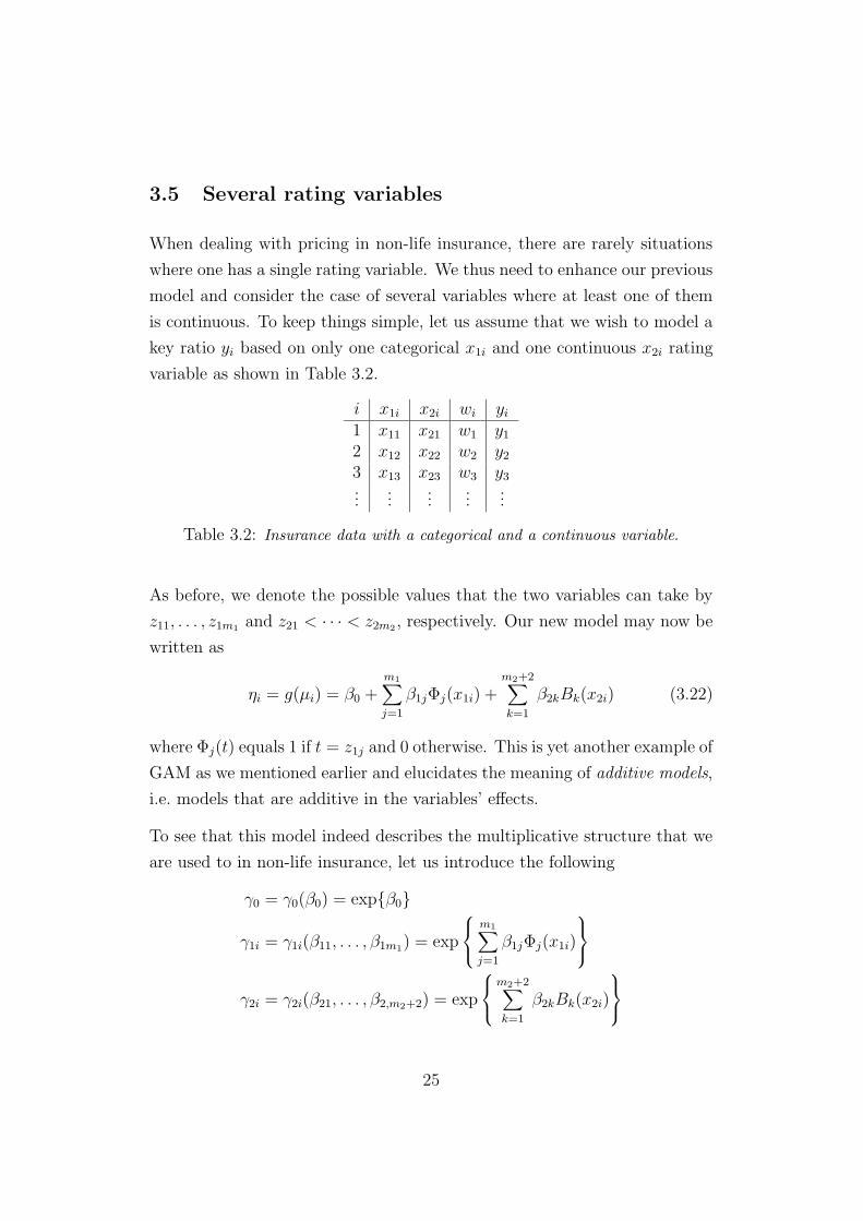
When dealing with pricing in non-life insurance, there are rarely situations

where one has a single rating variable. We thus need to enhance our previous

model and consider the case of several variables where at least one of them

is continuous. To keep things simple, let us assume that we wish to model a

key ratio yi based on only one categorical x1i and one continuous x2i rating

variable as shown in Table 3.2.

i x1i x2i wi yi

1 x11 x21 w1 y1

2 x12 x22 w2 y2

3 x13 x23 w3 y3...

......

......

Table 3.2: Insurance data with a categorical and a continuous variable.

As before, we denote the possible values that the two variables can take by

z11, . . . , z1m1 and z21 < · · · < z2m2 , respectively. Our new model may now be

written as

ηi = g(µi) = β0 +m1∑

j=1

β1jΦj(x1i) +m2+2∑

k=1

β2kBk(x2i) (3.22)

where Φj(t) equals 1 if t = z1j and 0 otherwise. This is yet another example of

GAM as we mentioned earlier and elucidates the meaning of additive models,

i.e. models that are additive in the variables’ effects.

To see that this model indeed describes the multiplicative structure that we

are used to in non-life insurance, let us introduce the following

γ0 = γ0(β0) = expβ0

γ1i = γ1i(β11, . . . , β1m1) = exp

m1∑

j=1

β1jΦj(x1i)

γ2i = γ2i(β21, . . . , β2,m2+2) = exp

m2+2∑

k=1

β2kBk(x2i)

25

Using the log-link and exponentiating, we see that the model (3.22) can be

rewritten on the familiar form

µi = γ0γ1iγ2i

A key question is now how to estimate the β-parameters in this model. One

commonly suggested strategy in additive models is to bring back the estima-

tion problem to the situation with a single rating variable. To illustrate this

backfitting algorithm, let us assume that the key ratio that we wish to model

is the claim frequency. The deviance may then be written as

D = 2∑

i

wi

(

yi log yi − yi log µi − yi + µi

)

= 2∑

i

wi

(

yi log yi − yi log(γ0γ1iγ2i) − yi + γ0γ1iγ2i

)

= 2∑

i

wiγ0γ1i

(

yi

γ0γ1i

logyi

γ0γ1i

−yi

γ0γ1i

log γ2i −yi

γ0γ1i

+ γ2i

)

Now, suppose that β0 and β11, . . . , β1m1 are considered as known. Conse-

quently,

w′′

i := wiγ0(β0)γ1i(β11, . . . , β1m1), y′′

i :=yi

γ0(β0)γ1i(β11, . . . , β1m1)

are also known and we get the following penalized deviance

∆ = 2∑

i

w′′

i

(

y′′

i log y′′

i − y′′

i log γ2i − y′′

i + γ2i

)

+ λm2+2∑

j=1

m2+2∑

k=1

β2jβ2kΩjk

Here, we see that this is the same estimation problem as in the previous sec-

tion and we can thus apply the above smoothing spline technique to estimate

the unknown parameters β21, . . . , β2,m2+2.

Let us now instead consider β0 and β21, . . . , β2,m2+2 as given. As above, we

define

w′

i = wiγ0(β0)γ2i(β21, . . . , β2,m2+2), y′

i =yi

γ0(β0)γ2i(β21, . . . , β2,m2+2)

and obtain the following penalized deviance

∆ = 2∑

i

w′

i

(

y′

i log y′

i − y′

i log γ1i − y′

i + γ1i

)

+ λm2+2∑

j=1

m2+2∑

k=1

β2jβ2kΩjk

26

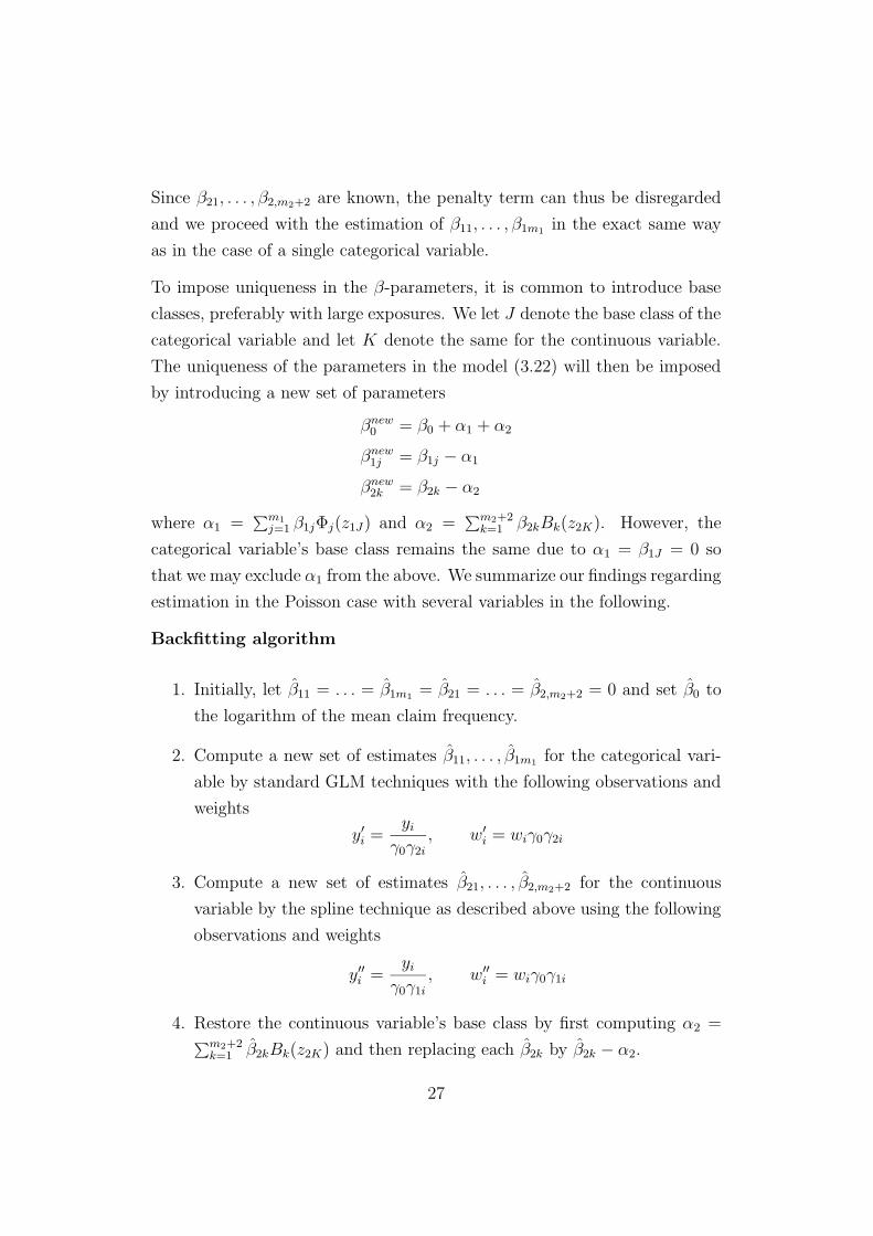
Since β21, . . . , β2,m2+2 are known, the penalty term can thus be disregarded

and we proceed with the estimation of β11, . . . , β1m1 in the exact same way

as in the case of a single categorical variable.

To impose uniqueness in the β-parameters, it is common to introduce base

classes, preferably with large exposures. We let J denote the base class of the

categorical variable and let K denote the same for the continuous variable.

The uniqueness of the parameters in the model (3.22) will then be imposed

by introducing a new set of parameters

βnew0 = β0 + α1 + α2

βnew1j = β1j − α1

βnew2k = β2k − α2

where α1 =∑m1

j=1 β1jΦj(z1J) and α2 =∑m2+2

k=1 β2kBk(z2K). However, the

categorical variable’s base class remains the same due to α1 = β1J = 0 so

that we may exclude α1 from the above. We summarize our findings regarding

estimation in the Poisson case with several variables in the following.

Backfitting algorithm

1. Initially, let β11 = . . . = β1m1 = β21 = . . . = β2,m2+2 = 0 and set β0 to

the logarithm of the mean claim frequency.

2. Compute a new set of estimates β11, . . . , β1m1 for the categorical vari-

able by standard GLM techniques with the following observations and

weights

y′

i =yi

γ0γ2i

, w′

i = wiγ0γ2i

3. Compute a new set of estimates β21, . . . , β2,m2+2 for the continuous

variable by the spline technique as described above using the following

observations and weights

y′′

i =yi

γ0γ1i

, w′′

i = wiγ0γ1i

4. Restore the continuous variable’s base class by first computing α2 =∑m2+2

k=1 β2kBk(z2K) and then replacing each β2k by β2k − α2.

27

5. Update the estimate β0 with β0 + α2.

6. Repeat Step 2–5 until convergence is reached.

Observe that in Step 2, 3 and 5, we use the preceding iteration’s β-estimates

to compute the new ones. In connection with the case studies it will be in-

structive to plot the fitted spline together with the partial residuals yi/(γ0γ1i).

Regarding the gamma case, it is easy to show that it is completely analogous

to the Poisson case apart from the weights that remain unchanged.

3.6 Interaction between a continuous and a categorical

variable

In the previous section, we used a model of the means µi based on a number

of rating variables, defined by

ηi = g(µi) = β0 +∑

p

fp(xpi)

where the univariate functions fp(xpi) are expressed in a different fashion

depending on whether the variable xpi is continuous or categorical

fp(xpi) =

mp∑

j=1

βpjΦj(xpi), xpi categorical

mp+2∑

k=1

βpkBk(xpi), xpi continuous

A model of this form provides the opportunity to examine the individual

variables’ effects separately and then simply add them together. Sometimes,

however, we encounter two variables that interact with each other so that the

above additivity assumption is no longer a reasonable one. Thus, instead of

modelling the effects of the two variables x1i and x2i separately, we wish to

consider their joint effect as f12(x1i, x2i). How to model f12(x1i, x2i) depends

highly on whether both of the variables are continuous or only one of them.

The case with interaction between two continuous variables is rather inter-

esting since it involves fitting a smooth surface to the data. Another possible

28

use that could be of interest for the insurance companies is to model geo-

graphical effects with the two continuous variables longitude and latitude.

In the past decades, there has been extensive work on how to define bivari-

ate (and multivariate) splines. This has resulted in a number of methods,

tensor-product splines, thin-plate splines, splines on triangulations etc. They

are all quite different from each other in both their construction and appli-

cation, though most of them require a relatively high technical level. There

are several excellent books that include this topic and the interested reader

is referred to Hastie and Tibshirani (1990), Dierckx (1993) and Green and

Silverman (1994). However, in this thesis, we will not pursue this topic any

further.

A considerably easier problem arises when one of the interacting variables is

categorical. A well-known example from motor insurance is the interaction

between policyholder sex and age — young male drivers are more accident

prone than the female drivers of the same age, whereas this phenomenon

fades out at higher ages. Here, we cannot simply multiply the effects of sex

and age, since this would imply that we have same ratio between the male

and female drivers irrespective of age. Instead, we wish to fit a separate

smoothing spline for each level of the categorical variable. In the motor

insurance example, we would thus obtain one spline fit for men and one for

women, which seems more natural considering the observed pattern.

To formulate a model, suppose we have the same situation as in section 3.5.

Thus, we have at our disposal one categorical variable x1i with the possible

values z11, . . . , z1m1 and a continuous one taking values z21, . . . , z2m2 . Further-

more, let βjk denote the parameters of the jth spline sj(t) =∑m2+2

k=1 βjkBk(t),

j = 1, . . . ,m1. We now have the following model for the interacting variables

ηi = η(x1i, x2i) =

s1(x2i), x1i = z11

...

sm1(x2i), x1i = z1m1

Note that this may also be expressed as

ηi = η(x1i, x2i) =m1∑

j=1

m2+2∑

k=1

βjkΦj(x1i)Bk(x2i)

29

where Φj(t) equals 1 if t = z1j and 0 otherwise; compare this model with (3.22).

Let us first consider the Poisson case with log link, i.e. µi = µ(x1i, x2i) =

expηi. We are now fitting m1 splines that may possibly be completely

different with regard to their shape and smoothing parameter. This leads to

the penalized deviance

∆ = 2∑

i

wi

(

yi log yi − yi log µi − yi + µi

)

+m1∑

j=1

λj

∫

(

s′′j (t))2

dt

where λ1, . . . , λm1 denote the smoothing parameters. Note that the new

penalty term is a sum of penalty terms, one for each spline.

In accordance with section 3.3, we let Ijk denote the set of all i for which

x1i = z1j and x2i = z2j. We may then define the aggregated weights wjk and

observations yjk as

wjk =∑

i∈Ijk

wi, yjk =1

wjk

∑

i∈Ijk

wiyi

Using that µi = expsj(z2k) = exp

∑m2+2`=1 βj`B`(z2k)

when i ∈ Ijk, the

above penalized deviance may thus be written as

∆ = 2m1∑

j=1

m2∑

k=1

wjk

yjk log yjk − yjk

m2+2∑

`=1

βj`B`(z2k) − yjk

+ exp

m2+2∑

`=1

βj`B`(z2k)

+m1∑

j=1

λj

m2+2∑

k=1

m2+2∑

`=1

βjkβj`Ωk`

Proceeding in the customary manner by setting the partial derivatives ∂∆/∂βrs

to zero, we obtain the following system of equations for each r = 1, . . . ,m1

−m2∑

k=1

wrkyrkBs(z2k) +m2∑

k=1

wrkBs(z2k) exp

m2+2∑

`=1

βr`B`(z2k)

+ λr

m2+2∑

`=1

βr`Ω`s = 0, s = 1, . . . ,m2 + 2

If we compare these to the equations in (3.16), we see that for each r =

1, . . . ,m1, we face the same estimation problem as in section 3.3, where we

30

had only one rating variable. The procedure is thus to aggregate the data

for each possible value of the categorical variable and then separately fit the

m1 splines, with the rth one being fitted to the observations yrk with the

associated weights wrk. It is also easily realized that the same procedure

applies to the gamma case as well.

Regarding several rating variables (in addition to the interacting ones), the

backfitting algorithm from the previous section extends naturally to include

interaction terms as well. When computing a new set of estimates for the

non-interacting variables, we use the following component for the interacting

variables, as if they were a single variable

γ12,i = γ12,i(β11, . . . , βm1,m2+2) = exp

m1∑

j=1

m2+2∑

k=1

βjkΦj(x1i)Bk(x2i)

Then, the procedure described in this section is used to compute a new

set of estimates β11, . . . , βm1,m2+2 for the interacting variables, using all the

other variables’ components to compute the observations and weights. Fi-

nally, we impose uniqueness in the parameters by analogously subtract-

ing α12 =∑m1

j=1

∑m2+2k=1 βjkΦj(z1J)Bk(z2K) =

∑m2+2k=1 βJkBk(z2K) = sJ(z2K),

where (J,K) is the base class for the compound variable.

4 Case studies

This section aims at evaluating the use of smoothing splines in the pricing

of motor insurances, and at our disposal we have policy and claims data

from Lansforsakringar insurance group over a period of 5 years. In order

to get a comprehensive picture, three types of motor vehicles and insurance

covers are studied. Our first case deals with a comparatively small portfolio

involving theft insurance for mopeds (Moped). In the second example we

analyze a somewhat larger portfolio of motor third-party liability insurance

for light lorries (Lorry). Finally, we conclude the case studies by exploring

the methods from section 3.6 on hull insurance for the largest single class of

motor vehicles, namely private cars (Car).

31

When dealing with GAM and in particular smoothing splines, the visual as-

sessment is an essential part of the fitting process. Therefore, in the following

examples we will encounter a large number of figures and in order to facil-

itate the reading of them, we will keep the same structure throughout. To

begin with, in those cases where we analyze only a single (continuous) rating

variable, the top and middle plots will show the fits concerning the claim

frequency and claim severity, respectively. The product of these two, i.e. the

risk premium, is then presented in the bottom plot. Regarding several rating

variables, the partial residuals will be shown instead.

This section will also serve as an evaluation of the CV method described in

section 3.4. It turns out that in most of the cases it produces a reasonable fit

for the smoothing spline or at least provides a decent start on where to look

for the ideal λ. Thus, unless otherwise mentioned, the CV-based smoothing

parameter is used in all the spline fits in the figures.

4.1 Moped

Up to now we have discussed quite a lot the drawbacks of polynomial re-

gression and this will be further illustrated here. However, there has been

very little discussion on the interval subdivision method which we intend to

remedy with this case.

The readers familiar with the Moped example in Ohlsson and Johansson

(2008) will recall that one of the rating variables there was Vehicle age.

This in fact continuous variable was, as always in traditional pricing with

GLM, treated as a categorical rating factor, and divided into two levels. Here,

we will use the full potential of Vehicle age by treating it as the continuous

variable it is and to begin with, we shall investigate the effect of Vehicle

age up to 25 years. Figure 4.1 shows the observed key ratios together with

the fits of the smoothing spline and interval subdivision method. We see

that both the claim frequency and severity behave quite stably and thus

do not pose any difficulties for the smoothing splines to capture the trends.

However, moving on to the interval subdivision method, finding a satisfactory

32

subdivision turns out to be anything but simple. One thing is clear though,

in order for the methods to be at all comparable, we have to use a large

number of intervals. With the subdivision as shown in Figure 4.1, we see

that the risk premium of a 2-year-old moped is nearly half the risk premium

of a 1-year-old. Now, is it really that the 1-year-old mopeds run double the

risk of theft as 2-year-old or is it simply the chosen subdivision or rather the

weaknesses of the method that result in such a conclusion? We realize that

if the interval subdivision method’s fit is to have any chance of following the

steep observations to the left in the plots, we would need to assign one level

for each Vehicle age, but then each class will contain fewer observations,

resulting in decreased precision. Thus, even in simple cases such as this, it is

hard to see how one could use the interval subdivision method in a judicious

way.

Figure 4.2 is similar to Figure 4.1, except that here the fit of the polynomial

regression of 10th degree is compared to the smoothing spline’s. What is

striking about these plots are the almost identical fits that these two meth-

ods produce, apart from maybe the claim severity where the polynomial fit

slightly begins to wiggle on the right side. Overall, both models provide an

adequate fit to the data.

Nevertheless, the real strength of the smoothing spline method over polyno-

mial regression is illustrated in Figure 4.3 where we extend the analysis to

include the far more sparse data for Vehicle age between 26 and 90 years.

The unpredictable behavior of the polynomial fit at high ages is scarcely

substantiated by the data and is beyond doubt caused by the method it-

self in addition to the choice of the polynomial degree. In the light of the

previous section we realize that the perhaps biggest problem when fitting a

polynomial is the sometimes drastic changes in the shape of the curve when

one increases or decreases the degree of the polynomial; recall Figure 1.2.

Smoothing splines, on the other hand, have the benefit of a continuous pa-

rameter, incorporated in the model, that affects the shape of the fitting

function in a smooth fashion. We see in Figure 4.3 that the smoothing spline

fit is stable even in the sparse region and gives a far more likely description

33

of the trend for older mopeds.

We have now reached a point at which we feel that there is no point to

continue comparing interval subdivision method and polynomial regression

to smoothing splines. We have convinced ourselves that the spline technique

is superior to the two competing methods. Hence, in the rest of this paper,

our full focus will be on splines and different issues concerning them.

Our final example in the Moped study illustrates the backfitting algorithm

from section 3.5. Again we refer to the Moped example in Ohlsson and

Johansson (2008) and add the remaining rating factors there, Vehicle class

and Geographic zone with 2 and 7 levels, respectively. Thus, we have one

continuous (Vehicle age) and two categorical variables which means that

we get an additional step in the backfitting algorithm. Figure 4.4 displays

the smoothing spline fits to the partial residuals in the last iteration of the

backfitting algorithm. If we compare these to the plots from Figure 4.1 or 4.2,

we see that they are virtually the same. The only real difference is the scale

on the y-axes.

4.2 Lorry

Our second case concerns motor third-party liability for light lorries, and

studies the effect of two continuous variables, Vehicle age and Vehicle

weight. Starting with the first one, Figure 4.6 depicts the observed claim

frequency, severity and risk premium together with the smoothing spline

fits. We again truncate the variable when the exposure becomes to small, at

Vehicle age = 25. As in the Moped case, the observations are fairly steady

though perhaps a bit more volatile, in particular the observed claim sever-

ity. Nevertheless, the smoothing splines manage to capture the underlying

dynamics. In the claim severity case it is noteworthy that, when searching

for the λ minimizing CV , the search method’s upper limit is reached; it is in

other words a straight line that in this sense provides the best model for the

claim severity.

We have a negative trend for claim frequency. It appears that older lorries

34

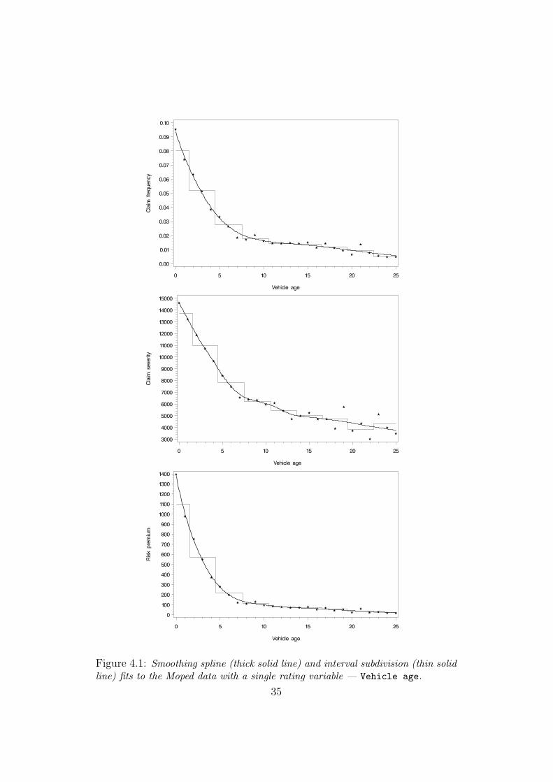
Figure 4.1: Smoothing spline (thick solid line) and interval subdivision (thin solidline) fits to the Moped data with a single rating variable — Vehicle age.

35

Figure 4.2: Smoothing spline (thick solid line) and degree 10 polynomial (thinsolid line) fits to the Moped data with a single rating variable — Vehicle age.

36

Figure 4.3: Smoothing spline (thick solid line) and degree 10 polynomial (thinsolid line) fits to the Moped data with a single rating variable — Vehicle age upto 90 years. 37

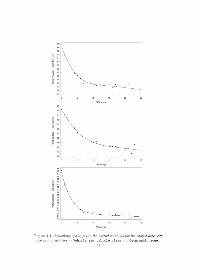
Figure 4.4: Smoothing spline fits to the partial residuals for the Moped data withthree rating variables — Vehicle age, Vehicle class and Geographic zone.

38

cause less traffic accidents than the newer ones. One possible explanation

for this lies in the less frequent use of older lorries in favor of the new ones,

whereas all motor vehicles in Sweden are obliged to have motor third-party

liability insurance by law. In the claim severity plot, we find that the overall

claims cost the same, irrespective of the age of the lorries.

We now move to Vehicle weight, where we have a considerably larger num-

ber of possible values, or knots. In the figures we have seen so far, we have

let the data decide upon an appropriate value of the smoothing parameter.

Due to the stability of those data though, one could just as well choose a

value by trial and error and would in all likelihood land close to the CV-

based λ. However, looking at the observed key ratios from the Lorry data in

Figure 4.7, we realize that it is practically impossible to smooth the highly

erratic observations with the naked eye. The smoothing splines shown in the

figure are yet again produced by the cross-validation technique which comes

extremely handy in this kind of situation.

Starting with the claim frequency case, we have a rather interesting shape

of the spline curve. If we would attempt to smooth the data by inspection,

our best surmise would probably be a slightly positively sloped straight line

through the observations. The smoothing spline, however, discerns a curve

with two humps from this cloud of observations. There are no known expla-

nations for this behavior, but one possibility would be that there are in fact

two or perhaps three different types of lorries that are present in the data.

All in all, it seems that the heavier lorries cause more traffic accidents.

Moving on to the claim severity, the smoothing spline manages to reveal some

underlying structure from the extremely volatile data. As with the Vehicle

age, the spline fit remains quite unaltered along Vehicle weight. We see

though that the average claim is somewhat more expensive for heavier lorries.

The essence is thus that neither the age nor the weight of a lorry affects the

average cost of a traffic accident substantially. A 1-ton lorry causes in average

almost equal damage as a 2-ton lorry, as well as a brand new or an old lorry.

Now, in practice, one would rarely analyze the effect of Vehicle weight

39

with all of its possible values, due to increased execution times. Instead, the

number of possible weights are reduced by rounding to the nearest 50 kg, for

instance, so that we end up with only a moderate number of knots. Figure 4.8

shows the smoothing spline fits for the Lorry data with this modified vari-

able Vehicle weight 50. What is most noticeable here is the remarkable

resemblance of the fitted splines from these two figures, despite the loss of

information this procedure could possibly entail. Another interesting feature

of this example is that for the claim frequency we do not have a unimodal

CV function which has been the case so far. If we look at the CV function

in the last iteration, shown in Figure 4.5, we see that there are in fact three

local minima. It is however the leftmost which is the global minimum leading

to a smoothing spline which almost interpolates the observations. Now, if

we choose λ as the third local minimum (log λ ≈ −3.5), we get the smooth-

ing spline fit to the claim frequency as shown in Figure 4.8. The conclusion

is that one must be cautious when fitting a smoothing spline and it is al-

ways a good idea to investigate the CV function, especially when there are

indications of multimodality.

Figure 4.5: CV curve for the smoothing spline fit to the claim frequency from theLorry data with a single rating variable — Vehicle weight 50.

40

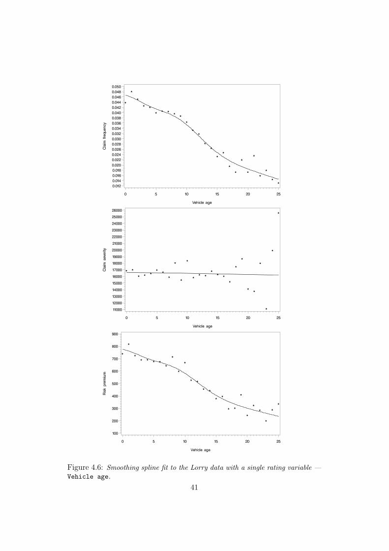
Figure 4.6: Smoothing spline fit to the Lorry data with a single rating variable —Vehicle age.

41

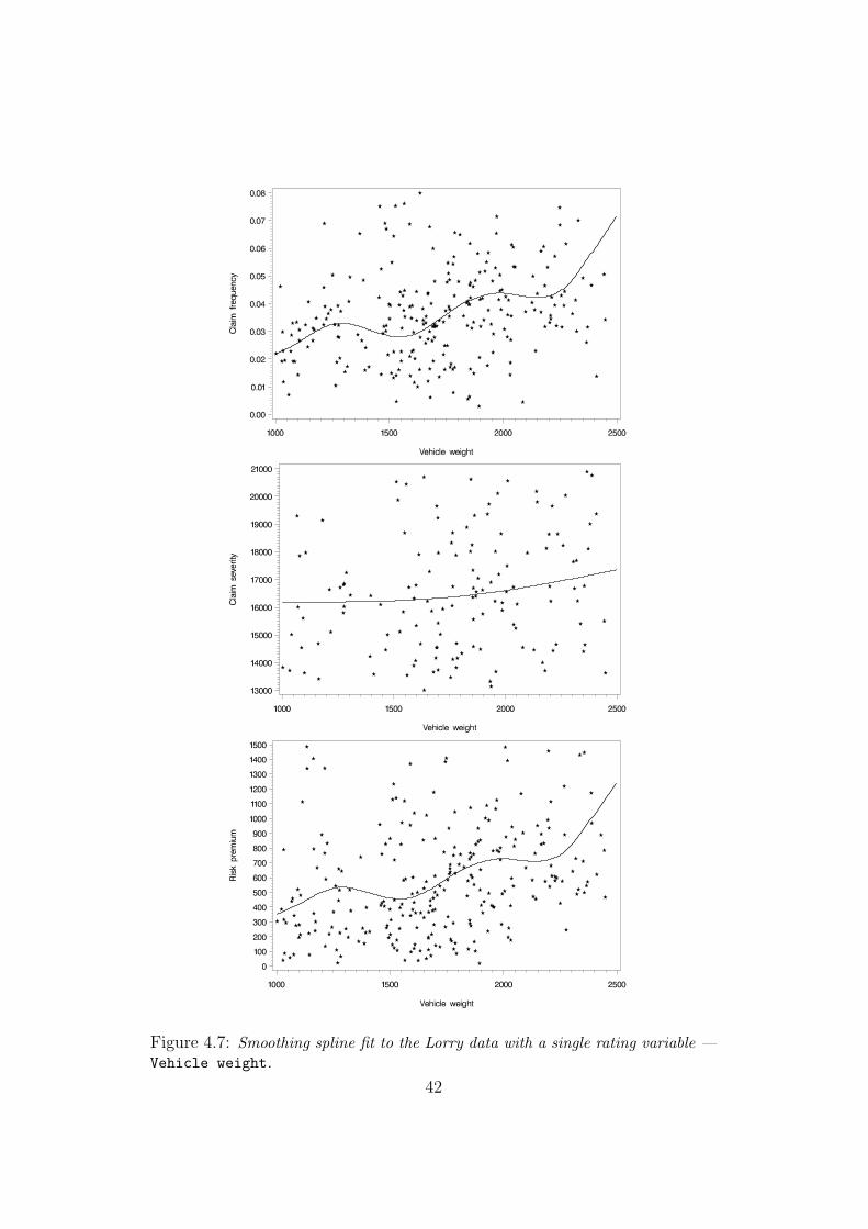
Figure 4.7: Smoothing spline fit to the Lorry data with a single rating variable —Vehicle weight.

42

Figure 4.8: Smoothing spline fit to the Lorry data with a single rating variable —Vehicle weight 50.

43

4.3 Car

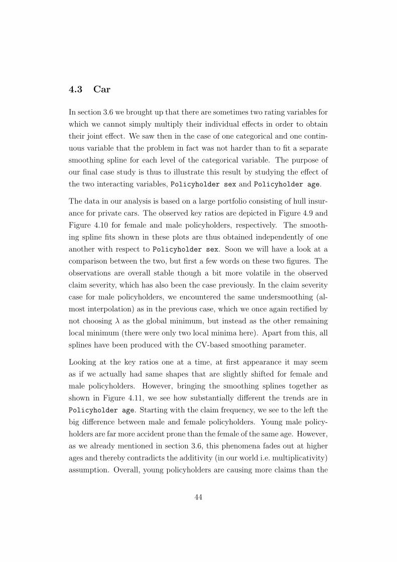
In section 3.6 we brought up that there are sometimes two rating variables for

which we cannot simply multiply their individual effects in order to obtain

their joint effect. We saw then in the case of one categorical and one contin-

uous variable that the problem in fact was not harder than to fit a separate

smoothing spline for each level of the categorical variable. The purpose of

our final case study is thus to illustrate this result by studying the effect of

the two interacting variables, Policyholder sex and Policyholder age.

The data in our analysis is based on a large portfolio consisting of hull insur-

ance for private cars. The observed key ratios are depicted in Figure 4.9 and

Figure 4.10 for female and male policyholders, respectively. The smooth-

ing spline fits shown in these plots are thus obtained independently of one

another with respect to Policyholder sex. Soon we will have a look at a

comparison between the two, but first a few words on these two figures. The

observations are overall stable though a bit more volatile in the observed

claim severity, which has also been the case previously. In the claim severity

case for male policyholders, we encountered the same undersmoothing (al-

most interpolation) as in the previous case, which we once again rectified by

not choosing λ as the global minimum, but instead as the other remaining

local minimum (there were only two local minima here). Apart from this, all

splines have been produced with the CV-based smoothing parameter.

Looking at the key ratios one at a time, at first appearance it may seem

as if we actually had same shapes that are slightly shifted for female and

male policyholders. However, bringing the smoothing splines together as

shown in Figure 4.11, we see how substantially different the trends are in

Policyholder age. Starting with the claim frequency, we see to the left the

big difference between male and female policyholders. Young male policy-

holders are far more accident prone than the female of the same age. However,

as we already mentioned in section 3.6, this phenomena fades out at higher

ages and thereby contradicts the additivity (in our world i.e. multiplicativity)

assumption. Overall, young policyholders are causing more claims than the

44

older. There is also a slight acclivitous trend among the older policyholders.

Regarding the claim severity, the younger policyholders’ claims cost more in

average than the older policyholders’. But overall it is the male policyholders

that cause the most expensive claims. This is likely due to that men in general

drive faster and more recklessly, but also because they own more expensive

cars with higher repair costs.

One conspicuous detail in all the plots that we have seen here is the hump

in the region around 45 years. This derives most likely from the fact that, in

this age interval, many policyholders are parents of teenage drivers to whom

they lend their cars. Here we can also discern a tendency of mothers lending

their cars to their children more often than the fathers. In addition we see

a slight displacement to right of the hump (and actually the whole curve)

for male policyholders relative to the female, confirming the well-recognized

fact that men become parents slightly after the women; this is perhaps best

envisioned in the claim severity plot.

45

Figure 4.9: Smoothing spline fits to the Car data with interaction betweenPolicyholder sex and Policyholder age. Female.

46

Figure 4.10: Smoothing spline fits to the Car data with interaction betweenPolicyholder sex and Policyholder age. Male.

47

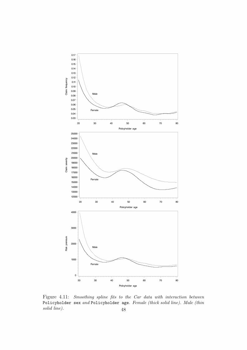
Figure 4.11: Smoothing spline fits to the Car data with interaction betweenPolicyholder sex and Policyholder age. Female (thick solid line). Male (thinsolid line). 48

5 Conclusions

The main objectives of this thesis were to investigate the theory and im-

plementation of smoothing splines and validate their usefulness in non-life

insurance pricing in various cases. For years, smoothing splines have been

successfully applied in a wide range of areas, but has not found their way

into the insurance business. In Sweden, the most likely reason is that the

topic is usually not covered in the basic courses in mathematical statistics.

Furthermore, many practitioners may find the spline theory difficult to di-

gest. In this thesis, we have shown how a cubic spline naturally arises as the

solution to a set of equations, not that different from the ones in the GLM

framework. The backfitting algorithm is section 3.5 enables simultaneous

analysis of both continuous and categorical variables, including the situa-

tions with interacting variables. In fact, the algorithm may be enhanced to

include multi-level factors (see Ohlsson and Johansson, 2008) as well, for a

complete rating analysis.

Another possible reason why the smoothing spline method has not been

used in connection with pricing is the lack of proper commercial software.

All large insurance companies in Sweden use SAS and the SAS procedure

for smoothing splines, Proc GAM, has limitations which prohibits its use

in rating problems. Therefore, we have made our own implementation of

smoothing splines carried out in SAS/IML.

In the case studies in section 4, smoothing splines turn out to perform very

well. Its superiority to the traditional interval subdivision method is obvi-

ous: one gets a more realistic model and gets rid of the jumps in the factors

and the tedious procedure of finding a satisfactory subdivision into inter-

vals. Polynomial regression performed better than was initially expected

after studying the literature on smoothing splines, but smoothing splines

were always better. In particular, the possibility of choosing the smoothing

parameter on a continuous scale instead of by discrete steps and the tendency

of polynomials to fluctuate at the edges make smoothing splines preferable.

In situations where it is necessary to choose a high degree of the polynomial

49

to produce a good fit, one may also encounter numerical problems. Admit-

tedly, the theory of polynomial regression is much simpler, but once one has

an implementation of smoothing splines, there is no reason to use polynomial

regression.

The cross validation approach for choosing the value of the smoothing param-

eter performed well in most situations, but sometimes encountered problems

when several local minima of the CV function existed. Our experience is

that it is always helpful to plot the CV function, but that the golden section

search used usually found the minimum rapidly. The value of the parameter

obtained by the CV method was not always in accordance with what would

seem reasonable from the plots of the fitted splines together with the partial

residuals. In such cases a manual adjustment of the smoothing parameter

may be needed, usually to increase the smoothing, since too large variations

are not accepted in a rating structure. If time had permitted, we would have

liked to compare the CV method with the much faster but less accurate GCV

(generalized cross validation) method.

50

6 References

A large portion of the thesis work consisted in learning SAS, during which

we used Carpenter (1998), Delwiche and Slaughter (1995), and the documen-

tation from SAS Institute Inc. among the references below.

Brockman, M.J. and Wright, T.S. (1992) Statistical motor rating:

making effective use of your data. Journal of the Institute of Actuaries 119,

III, 457–543.

Carpenter, A. (1998) Carpenter’s Complete Guide to the SAS Macro Lan-

guage. Cary, NC: SAS Institute Inc.

Curry, H.B. and Schoenberg, I.J. (1947) On spline distributions and

their limits: the Polya distribution functions. Bulletin of the American Math-

ematical Society 53, 1114.

Delwiche, L.D. and Slaughter, S.J. (1995) The Little SAS Book: A

Primer. Cary, NC: SAS Institute Inc.

Dierckx, P. (1993) Curve and Surface Fitting with Splines. Oxford Uni-

versity Press.

Eriksson, G. (2002) Numeriska Algoritmer med Matlab. Nada, KTH.

Green, P.J. and Silverman, B.W. (1994) Nonparametric Regression

and Generalized Linear Models: A Roughness Penalty Approach. Chapman

& Hall.

Hastie, T.J. and Tibshirani, R.J. (1990) Generalized Additive Models.

Chapman & Hall/CRC.

Hutchinson, M.F. and de Hoog, F.R. (1985) Smoothing noisy data

with spline functions. Numerische Mathematik 47, 99–106.

McCullagh, P. and Nelder, J.A. (1989) Generalized Linear Models,

Second Edition. Chapman & Hall/CRC.

51

Ohlsson, E. and Johansson, B. (2008) Non-Life Insurance Rating using

Generalized Linear Models, Fifth Edition. Matematisk Statistik, Stockholms

Universitet.

Ruppert, D., Wand, M.P. and Carroll, R.J. (2003) Semiparametric

Regression. Cambridge University Press.

SAS Institute Inc. (1989) SAS r©Guide to the SQL Procedure: Usage and

Reference, Version 6, First Edition. Cary, NC: SAS Institute Inc.

SAS Institute Inc. (1989) SAS r©Language and Procedures: Usage, Ver-

sion 6, First Edition. Cary, NC: SAS Institute Inc.

SAS Institute Inc. (1991) SAS/GRAPH r©Software: Usage, Version 6, First

Edition. Cary, NC: SAS Institute Inc.

SAS Institute Inc. (1997) SAS r©Macro Language: Reference, First Edi-

tion. Cary, NC: SAS Institute Inc.

SAS Institute Inc. (1999) SAS/IML r©User’s Guide, Version 8. Cary,

NC: SAS Institute Inc.

SAS Institute Inc. (1999) SAS/STAT r©User’s Guide, Version 8. Cary,

NC: SAS Institute Inc.

Schoenberg, I.J. (1946) Contributions to the problem of approximation

of equidistant data by analytic functions. Quarterly of Applied Mathematics

4, 45–99, 112–141.

52