1

MATHEMATICAL MODELLING FOR ADVANCED TECHNOLOGIES

by G. Cavuoti, G. Bedetti and E. Filippi

Casale Group Via Pocobelli 6 – Lugano – Switzerland

ABSTRACT

The Casale Group is a dynamic and innovative company deeply involved in

researching and developing new advanced technologies for chemical processes.

The Group possesses the ultimate tools to gain competitive advantages and the

capability to accurately and reliably simulate new flow sheeting solutions, new

equipment and unusual operating conditions.

In this perspective, the Casale R&D Department has developed a set of new

powerful mathematical models with relevant easy-to-use computer software, in

order to simulate highly complex equipment geometries and flow-sheet

architectures.

This paper will illustrate our achievements in the:

1. flow sheeting simulation of urea plants;

2. 3D multiphase simulation of fixed bed plate-cooled catalytic reactors.

2

1. ADULA – THE SIMPLEST WAY TO UREA PLANT FLOW-SHEETING Simulation of Urea Plant flow-sheets face a lack of calculation tools and thermodynamic data. Urea Casale is a company that operates already for many years in this field and can get direct information feedback from Urea plants. On the basis of this “experimental” data, we have developed a complete software suite to simulate any flow-sheet configuration of a urea plant.

Fig. 1.1 – Adula Overview Graphic Interface

The Calculation Engine The simulation of each piece of equipment is performed by means of only two calculation engines: 1) chemical reactive two-perfectly-mixed-phase flash calculation 2) chemical reactive two-phase plug flow calculation not in bulk phase VLE

equilibrium. These two calculation modules, with the appropriate constitutive equations for thermodynamic and transport properties for each phase and flow regimes, are capable to simulate almost all the equipment of a complete Urea Plant. To simulate countercurrent units that involve basically a boundary condition problem, we adopt not a shooting algorithm, but a segregate-phase solving approach (each phase is solved at once fixing the parameter of the other phase). In this manner we get the benefit in terms of calculation time and stability, also for pieces of equipment that are intrinsically countercurrent stages units, such as distillation columns. The computer code of the calculation engine is written in Fortran90.

3

Thermodynamic and Transport Properties Thermodynamic properties (volumetric, caloric, and VLE partition coefficient) are derived from a proprietary hybrid molecular-ionic formulation of the six component urea system: ammonia, carbon dioxide, urea, water, ammonium carbamate, ammonium bicarbonate (1, 2). The transport properties of single components and mixtures are calculated on the base suggested in Poling-Prausnitz-O'Connell – The Properties of Gases and Liquids – V ed. (3, 4). Formulas for macroscopic transport coefficients, (Nusselt number, Sherwood number, Fanning factor), are collected for all the geometries (falling film, bubble column and two (one) flow regimes of interest. (5-12). The preference is accorded to those formulations that are in agreement with Colburn analogy. The Overall Mass & Energy Balance Solver The two pieces of equipment solving engines are embedded in an overall mass and energy balance powerful solver that considers each equipment as a component specific multi-splitter (Nagiev-Rosen) (13-15). The generation terms are considered as virtual feed stream. In this way the solving path always respects the mass balance with no need of convergence block. During the iteration sequence the algorithm only modifies the splitting factor of each piece of equipment and chemical component; convergence is reached not by minimizing the tearing streams, but by minimizing the splitting factor variation. The Graphic User Interface Finally, we chose to envelope the Adula flow-sheet simulator in a familiar, easy-to-use and modify environment, such as Microsoft Excel used as a Graphic User Interface. The GUI code is thus written in VisualBasic for Application, and uses the Excel worksheets as a sort of powerful VisualBasic control. Adula lives and coexists with all the other spreadsheet-based applications in a well-known frame without the need to read and learn anything about the lot of trivial commands related to edit, modify, print, copy & paste of flowsheet pieces, reports, etc., but also with the more complex auxiliary user-customized calculations and spreadsheet optimizations. The operative manual of Adula is thus reduced to a few pages.

4

1.2 MAIN EQUATION SET

( )

( )

⎪⎪⎪

⎩

⎪⎪⎪

⎨

⎧

⋅≡

ℜ=

=

⎪⎪⎩

⎪⎪⎨

⎧

′⋅⋅′′+−⋅′⋅=

′⋅⋅′′+−⋅′⋅=

⎪⎪⎩

⎪⎪⎨

⎧

′⋅′′=

⋅+′⋅′′=

∑

∏

=

=

•

•

bulk phase liquidin reactionsfor balanceelement

bulkphase liquidin reactions slow of ratereaction

bulk phase liquidin reactionsfast for equilibria chemical

phase gas of balanceenthalpy

phase liquid of balanceenthalpy

phase gasin balance mass

phase liquidin balances mass

1

)''(')''('

)''('1

)''('

)7

),,()6

)5

ˆ)4

ˆ)3

)2

)1

R

rririigLi

Lrrr

I

iirr

IIGIGGIIGG

IJLILLIJLL

IiIGiG

i

tLigLIiILiL

i

LL

L

ir

L

Mm

xpT

xK

SHmTTShdzHd

SHmTTShdzHd

Smdzmd

SmSmdzmd

ξν

ξ

ν

&&

&

&&

&&

&&

&&&

( ) ( )( )( )

⎪⎪⎪⎪⎪⎪⎪

⎩

⎪⎪⎪⎪⎪⎪⎪

⎨

⎧

′′⋅≡′′

==

⋅=−⋅+⋅′′=′′

−⋅+⋅′′=′′

−⋅+−⋅=⋅′′+⋅′′

=′′+′′

∑

∏

=

=

•

•

••

reactions interf.for on conservatielement ofequation

interfaceat reactionsfast for equilibria chemical

interface liquid-gasat Equilibria LiquidVapor

flux gas-interfacefor equation veconstituti

flux liquid-interfacefor equations veconstituti

interface liquid-gasat balanceenthalpy

interface liquid-gasat balancesmolar

1

1

)14

,1)13

)12)11

)10

ˆˆ)9

0)8

I

ir

R

rririigIi

I

iIiIrr

LiIiIGiIi

GiGiIiGGiIIGiIGi

LiLiIiLLiIILiILi

IGGILLIGIGILIL

iILiIGi

Mm

RrxK

Kknm

kmm

TThTThHmHm

mm

ξν

ωωωωω

ωωω

ν

&&

&&

&&

&&

&&

( )

( )

tGGLL

frTPGGGGLLLL

GGLbeGLLG

GtGGG

LtLLL

Smv

dzvv

Kdpgdhdvvdvv

DvvvSvmSvm

ρρερερ

ρρρερε

ερρερερ

&

&

&

≡+≡

⎪⎪⎪

⎩

⎪⎪⎪

⎨

⎧

=′++++

=−≡≡

eq.)(Bernoulli balance momentum overall

bal. momentum liquid and gas from eq. velocity slip

velocitygas average of definition

velocityliquid average of definition

02

)18

,,,)17)16)15

5

⎪⎪⎪⎪

⎩

⎪⎪⎪⎪

⎨

⎧

=

=

⎟⎟⎠

⎞⎜⎜⎝

⎛⋅=

⋅=′

≡′′′

plate perforated fromout coming bubble of size initialfor equation

geometry bubblefor equation

e)coalescenc (nodiameter av. bubblefor equation

volumeoverall ofunit per area interface liq.-gas

(...))22

(...))21

)20

6)19

0

3/1

0

00

fD

fSS

mm

DD

SS

DSSS

be

Ibe

Ib

G

G

G

Gbebe

Ibe

IbG

bet

II

ρρ

ε

&

&

Nomenclature and SI units

h hL G• •, : interface heat exchange coeff. liquid(L), gas(G) side, corrected with overall mass flow(•) W/m²°C

& , &H HL G : enthalpy flow of liquid phase (L), gas phase (G) W ~ , ~H HiJL iIG : partial mass enthalpy of component i at interface, liquid side (IL), gas side (IG) J/mol

I : number of chemical components -

k kiL iG• •, : interface mass exchange coeff. liquid(L), gas(G) side, corrected with overall mass flow(•) mol/m²s

reqrr KKK γ/≡ : pseudo-equilibrium constant of reaction r -

KiI : gas-liquid partition constant of component i -

iGiL mm && , : mass flow of component i in liquid phase (L), gas phase (G) mol/s

iIGiIL mm ′′′′ && , : mass flux of component i from interface to liquid phase (IL), to gas phase (IG) mol/m²s

igIm ′′& : mass of component i generate (g) at gas-liquid interface (I) for unit of time and interface area mol/m²s

LigLm )''('& : mass of component i generate (g) in liquid phase bulk per unit of time and liquid volume mol/m3s

R : number of reactions -

IS ′ : gas-liquid interface area per unit of length m

′′′SI : gas-liquid interface area per unit of overall volume 1/m

S S StL tG t, , : cross-flow surface area of liquid (L), of gas (G), overall (t) m²

T TL G, : temperature of liquid phase (L), of gas phase (G) °C

IT : temperature of gas-liquid interface °C

v v vL G, , : effective average velocity of liquid phase (L), of gas phase (G), overall m/s

GiLi ωω , : mass fractions of component i in bulk liquid phase, in bulk gas phase -

GiILiI ωω , : mass fractions of component i at interface liquid phase side, at interface gas phase -

z : longitudinal coordinate of one-dimensional flow stream m ℜr : rate of chemical reaction r mol/m3s

ε εL G, : volumetric fraction of liquid phase (L), of gas phase (G) , (in control volume) -

ν ir : stechiometric coefficient of component i in chemical reaction r -

ρ ρ ρL G, , : density of liquid phase (L), gas phase (G), overall (in control volume) kg/m3

& ′′ξ r : reaction degree of interface reaction for unit of time e interfacial area (SI) mol/m²s

ξ rL(''')

: reaction degree of liquid bulk reaction for unit of time e liquid volume ((‘’’)L) mol/m3s

6

1.3 EXAMPLES

Fig. 1.2 – Adula Graphic Interface

Fig. 1.3 – Adula Urea Plant Flowsheet

LINE N°Description

phaseP [MPa a]

T [°C]kg/h %w kg/h %w kg/h %w kg/h %w kg/h %w kg/h %w kg/h %w kg/h %w kg/h %w

NH3 0 0.0 119789 65.8 65332 30.0 7042 54.7 59898 99.9 59886 49.1 40671 23.7 31709 53.5 45808 40.5CO2 48205 99.0 49444 27.2 31515 14.5 4871 37.8 0 0.0 49485 40.5 11568 6.7 24825 41.9 31427 27.8Urea 0 0.0 50 0.0 83652 38.4 0 0.0 0 0.0 50 0.0 83652 48.8 0 0.0 209 0.2H2O 0 0.0 12716 7.0 37332 17.1 461 3.6 61 0.1 12657 10.4 35611 20.8 2183 3.7 35670 31.5Inerts 498 1.0 0 0.0 0 0.0 498 3.9 0 0.0 0 0.0 0 0.0 498 0.8 0 0.0

TOTAL 48703 100.0 182000 100.0 217830 100.0 12872 100.0 59959 100.0 122078 100.0 171502 100.0 59216 100.0 113115 100.0M. W. [kg/kmol]

Viscosity [mPa*s]Density [kg/m3]Flow rate (m3/h)

LINE N°Description

phaseP [MPa a]

T [°C]kg/h %w kg/h %w kg/h %w kg/h %w kg/h %w kg/h %w kg/h %w kg/h %w kg/h %w

NH3 10934 40.5 34874 40.5 15886 33.1 18986 49.6 9314 40.5 1620 40.5 1736 72.4 16938 12.0 8958 7.0CO2 7502 27.8 23926 27.8 6712 14.0 17215 45.0 6390 27.8 1111 27.8 47 2.0 7532 5.3 3208 2.5Urea 50 0.2 159 0.2 159 0.3 0 0.0 43 0.2 7 0.2 0 0.0 83652 59.3 83652 65.8H2O 8514 31.5 27156 31.5 25180 52.5 1976 5.2 7253 31.5 1261 31.5 17 0.7 33010 23.4 31357 24.7Inerts 0 0.0 0 0.0 0 0.0 100 0.3 0 0.0 0 0.0 598 24.9 0 0.0 0 0.0

TOTAL 27000 100.0 86115 100.0 47937 100.0 38276 100.0 23000 100.0 4000 100.0 2398 100.0 141131 100.0 127175 100.0M. W. [kg/kmol]

Viscosity [mPa*s]Density [kg/m3]Flow rate (m3/h)

NOTE: The process conditions and flow quantities listed on this document are those expected and may be altered as required to produce the desired production rate and/or product quality

00 FIRST ISSUE LRU GDC AS 19.nov.07

REV. DESCRIPTION PREP'D CHECK'D APPR'D DATE

1077.0 109.5 1093.51077.0 1077.01004.6 858.2 128.1

28.5 22.0 23.60.00029451 0.000160734 0.000108968 2.14748E-05

Cbm to E-E3

98.0 155.0 155.014.80 14.80 14.80 1.80

LIQ LIQ

Cbm to E-E3/E-E4 Cbm to E-E1 Solution from E-E1 Vapors from E-E1 Cbm to E-E4 Vapors from S-D1 Urea sol. to E-E6 Urea sol. from S-D3

105.0

10 11 12 13 14 15 16 17 18

103.4 112.5 179.3 496.8178.3 213.7 221.6 104.2

28.6

273.1 851.7 982.9 123.6 579.9 1085.5 956.3 119.2 1077.0

17.0 39.2 31.2 23.143.8 27.5 33.0 22.7

30.8 171.5 202.1 191.8120.0 108.4 192.7 192.7

Cbm from P-G2A/S

15.70 15.70 15.70 15.70 23.30 14.80 14.80 14.80 14.80

NH3 to J-PJ101 Carbamate from S-D1 Urea sol. from E-E2 Vapors from E-E2CO2 to R-R1 NH3 & cbm to R-R1 R-R1 outlet R-R1 vapors

"IDR" UREA PLANT WITH MELAMINE - CAPACITY 2000 MTD1 2 3 4 5 6 7 8 9

SHEET For Line Number, refer to Process Flow Diagram N° 8494-10-E-PDG-3001 8494-10 PAGE 1 OF 5

SPEC.PROJECT : IDR PLANT REVAMPING 00 8494-10-E-PZQ-3001CUSTOMER : ZAKLADY AZOTOWE PULAWY - SPOLKA AKCYJENA REV

MATERIAL BALANCE JOB N°

LIQ

98.0

GAS LIQ LIQ GAS LIQ LIQ LIQ GAS

1085.2

LIQ LIQ LIQ GAS

14.80 14.80 14.80 14.80

28.6

2.5024E-05 0.00012827 0.000185931 2.15062E-05 0.000127464 0.000212253 0.000181642 2.12879E-05 0.00029451

25.1 85.7 55.9 298.8 21.4 3.7 21.9 129.1 117.2

0.0002945134.819.128.628.6

160.098.0

0.000403763

1.80140.298.0186.2199.5

1.94462E-050.00029451

LIQLIQGAS

0.00038101135.4

7

2. SECTOR3D - 3D SIMULATION OF FIXED BED, PLATE-COOLED CATALYTIC REACTORS In order to obtain accurate simulations of the fixed bed reactor performance, Casale has developed a fully 3D computer code to calculate velocity, pressure, temperature and composition fields in a fixed-bed reactor of any complex geometry. The code considers two (or more) phases, catalyst and reacting fluid, with the same eulerian approach. A graphic interface written in VisualBasic, allows the geometrical modeling of complex geometries and give the tools to impose boundary condition on surface and material property on volumes. Simplified graphic interfaces suitable for cylindrical geometries give the same capabilities in Excel in a simpler way.

Fig. 2.1 – The Sector3D Graphic Interface

The code algorithm is a finite volume – segregated variable type, as the one derived by Patankar and Spalding (SIMPLER method) (16-18), and directly integrates the overall mass balance (continuity eq.), momentum (Navier-Stokes), energy (Fourier eq.), single components mass balance (Fick) in each phase. The programming code language is Fortran90. Appropriate equations have been adopted for thermodynamic and transport properties (rheological and turbulent) and for momentum, heat and mass transfer coefficients at boundary limits. Accurate Casale proprietary chemical kinetics for ammonia and methanol synthesis have been developed and implemented for each chemical system of interest.

8

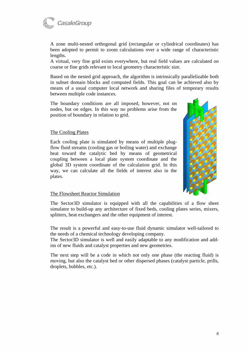
A zone multi-nested orthogonal grid (rectangular or cylindrical coordinates) has been adopted to permit to zoom calculations over a wide range of characteristic lengths. A virtual, very fine grid exists everywhere, but real field values are calculated on coarse or fine grids relevant to local geometry characteristic size. Based on the nested grid approach, the algorithm is intrinsically parallelizable both in subset domain blocks and computed fields. This goal can be achieved also by means of a usual computer local network and sharing files of temporary results between multiple code instances. The boundary conditions are all imposed, however, not on nodes, but on edges. In this way no problems arise from the position of boundary in relation to grid. The Cooling Plates Each cooling plate is simulated by means of multiple plug-flow fluid streams (cooling gas or boiling water) and exchange heat toward the catalytic bed by means of geometrical coupling between a local plate system coordinate and the global 3D system coordinate of the calculation grid. In this way, we can calculate all the fields of interest also in the plates. The Flowsheet Reactor Simulation The Sector3D simulator is equipped with all the capabilities of a flow sheet simulator to build-up any architecture of fixed beds, cooling plates series, mixers, splitters, heat exchangers and the other equipment of interest. The result is a powerful and easy-to-use fluid dynamic simulator well-tailored to the needs of a chemical technology developing company. The Sector3D simulator is well and easily adaptable to any modification and add-ins of new fluids and catalyst properties and new geometries. The next step will be a code in which not only one phase (the reacting fluid) is moving, but also the catalyst bed or other dispersed phases (catalyst particle, prills, droplets, bubbles, etc.).

9

2.1 SECTOR3D EXAMPLES

Fig. 2.2 – The Sector3D Flowsheet Interface

Fig. 2.3 – Radial Cooling Plates Ammonia Reactor

10

Fig. 2.4 – Radial Cooling Plates Methanol Reactor – Gas Temperature Field

Fig. 2.4 – Radial-Axial Cooling Plates Ammonia Reactor – Centerline

Temperature, Pressure, NH3 Composition, Particle Path Fields

11

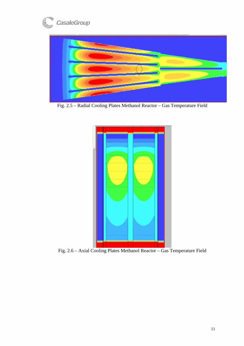
Fig. 2.5 – Radial Cooling Plates Methanol Reactor – Gas Temperature Field

Fig. 2.6 – Axial Cooling Plates Methanol Reactor – Gas Temperature Field

12

References 1) G.T.Chao – Urea its properties and manufacture – Chao’s Institute, 1967 2) IIR – NH3 – H2O Thermodynamic and physical properties – Int. Inst. of Refr., 1994 3) R.C.Reid, J.M.Prausnitz – The Properties of Gases & Liquids IV ed.– McGraw Hill, 1987 4) Poling-Prausnitz-O' Connell – The Properties of Gases and Liquids – V ed. 2000 5) W.M.Rohsenow, J.P.Hartnett - Handbook of Heat Transfer - McGraw Hill, 1973 6) M.Jakob - Heat Tranfer - John Wiley & Sons, 1957 7) J.C.Collier - Convective Boiling and Condensation - McGraw Hill, 1972 8) F.Kreith - Principi di Trasmissione del calore - Liguori Editore 9) G.Astarita, D.W.Savage, A.Bisio – Gas Treating with Chemical Solvents – John Wiley & Sons, 1983 10) V.M.Ramm – Absorptions of gases – Israel Program for Scientific Translations, 1968 11) I.E.Idelcick - Handbook of Hydraulic Resistence, II ed. - Springer-Verlag 12) R.H.Perry – D.W.Green - Chemical Engineers’ Handbook VII ed. – McGraw Hill, 1997 13) M.F.Nagiev – Recycle process in chemical engineering, Pergamon Press1964 14) E.J.Henley, E.M.Rosen, Material and Energy balance computation, Wiley, 1969 15) F.P.Foraboschi – Principi di Ingegneria Chimica – UTET, 1972 16) S.V.Patankar – Numerical Heat Transfer and Fluid Flow – McGraw Hill, 1980 17) R.B.Bird, et al. – Fenomeni di Trasporto – Ed. Ambrosiana, 1979 18) G.F.Froment, K.B.Bischoff - Chemical Reactor Analysis and Design - John Wiley & Sons, 1990 19) W.H.Press – Numerical Recipes in Fortran, II ed. – Cambridge Univ.Press, 1992 20) G.Buzzi-Ferraris – Numerical Methods in C++ - Addison-Wesley, 1998 21) V.Comincioli – Numerical Analysis – McGraw Hill, 1990 Lugano, March 2008 Code:pap/conf/amm/stm-8/stm-8 paper 2008