mathematical modeling, numerical computation, and applications of
TRANSCRIPT

Mathematical Modeling, Numerical Computation, and Applications ofNarrow Escape Problems
Alexei F. Cheviakov1
1University of Saskatchewan, Saskatoon, Canada
May 01, 2011
A. Cheviakov (UofS) Narrow Escape Problems May 01, 2011 1 / 23

Outline
1 IntroductionNarrow Escape ProblemsSome Known ResultsMatched Asymptotic Expansions
2 Asymptotic Results for the MFPTAsymptotic Results for 2D DomainsExamples: Disk and Square in 2D3D: the Sphere
3 Global Optimization of Trap LocationsThe Unit Sphere
4 Asymptotic MFPT Vs. Full Numerical SimulationTrap Size EffectsTrap Separation Effects
5 Conclusions
A. Cheviakov (UofS) Narrow Escape Problems May 01, 2011 2 / 23

Collaborators
Michael Ward, University of British Columbia, Vancouver, Canada
Ronny Straube, Max-Planck Institute for Dynamics of Complex Technical Systems,Magdeburg, Germany
Raymond Spiteri, University of Saskatchewan, Saskatoon
Ashton Reimer, summer USRA student, University of Saskatchewan, Saskatoon
A. Cheviakov (UofS) Narrow Escape Problems May 01, 2011 3 / 23
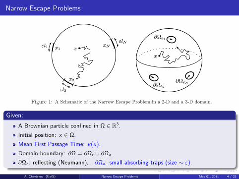
Narrow Escape Problems
Figure 1: A Schematic of the Narrow Escape Problem in a 2-D and a 3-D domain.
Given:
A Brownian particle confined in Ω ∈ R3.
Initial position: x ∈ Ω.
Mean First Passage Time: v(x).
Domain boundary: ∂Ω = ∂Ωr ∪ ∂Ωa.
∂Ωr : reflecting (Neumann), ∂Ωa: small absorbing traps (size ∼ ε).
A. Cheviakov (UofS) Narrow Escape Problems May 01, 2011 4 / 23

Narrow Escape Problems
Figure 1: A Schematic of the Narrow Escape Problem in a 2-D and a 3-D domain.
Problem for MFPT: 4v = − 1
D, x ∈ Ω ,
v = 0, x ∈ ∂Ωa; ∂nv = 0, x ∈ ∂Ωr .
(1)
Average MFPT: v =1
|Ω|
∫Ω
v(x) dx = const.
A. Cheviakov (UofS) Narrow Escape Problems May 01, 2011 4 / 23

Applications of Narrow Escape Problems
Examples of applications:
Pores of cell nuclei
Synaptic receptors on dendrites
Pores of cell membranes
Mathematical Modelling of Narrow Escape ProblemsAshton S. Reimer and Alexei F. Cheviakov
Department of Mathematics and Statistics, University of Saskatchewan
The Narrow Escape Problem
The narrow escape problem concerns the motion of a Brownian particle confined in a bounded domain Ω ∈ Rd (d = 2, 3 in twoor three space dimensions) whose boundary ∂Ω = ∂Ωr
⋃∂Ωa is almost entirely reflecting (∂Ωr), except for small windows (traps,
∂Ωa), through which the particle can escape.
Applications
Pores in cell nuclei: Synaptic receptors on dendrites: Ion channels in cell membranes:
The Mathematical Model
The mean first passage time (MFPT), v(x), is defined as theexpectation value of the time taken for a Brownian particle starting initiallyfrom some point x in a domain Ω to escape through any window on theboundary ∂Ω. To find v(x), one must solve the
Dirichlet-Neumann boundary problem for MFPT v(x):
4v = − 1D, x ∈ Ω ,
v = 0, x ∈ ∂Ωa =N⋃
j=1∂Ωεj
; ∂nv = 0, x ∈ ∂Ωr.(1)
Where D is the diffusivity coefficient (D = const or D = D(x)). A usefulquantity is the average MFPT defined as v.
I Average MFPT:
v = 1|Ω|
∫
Ωv(x) dx = const. (2)
Copyright © by SIAM. Unauthorized reproduction of this article is prohibited.
804 S. PILLAY, M. WARD, A. PEIRCE, AND T. KOLOKOLNIKOV
problem in the limit when the measure of the absorbing set |∂Ωa| = O(ε) is asymp-totically small, where 0 < ε 1 measures the dimensionless radius of an absorbingwindow.
It is well known (cf. [10], [15], [16]) that the MFPT v(x) satisfies a Poissonequation with mixed Dirichlet–Neumann boundary conditions, formulated as
v = − 1D
, x ∈ Ω ,(1.1a)
v = 0 , x ∈ ∂Ωa =N⋃
j=1
∂Ωεj , j = 1, . . . , N ; ∂nv = 0 , x ∈ ∂Ωr ,(1.1b)
where D is the diffusion coefficient associated with the underlying Brownian motion.In (1.1), the absorbing set consists of N small disjoint absorbing windows ∂Ωεj cen-tered at xj ∈ ∂Ω (see Figure 1). In our two-dimensional setting, we assume that thelength of each absorbing arc is |∂Ω| = εlj, where lj = O(1). It is further assumedthat the windows are well separated in the sense that |xi − xj | = O(1) for all i = j.With respect to a uniform distribution of initial points x ∈ Ω, the average MFPT,denoted by v, is defined by
(1.2) v = χ ≡ 1|Ω|
∫
Ω
v(x) dx ,
where |Ω| denotes the area of Ω.
Fig. 1. Sketch of a Brownian trajectory in the two-dimensional unit disk with absorbing windowson the boundary.
Since the MFPT diverges as ε → 0, the calculation of the MFPT v(x), and thatof the average MFPT v, constitutes a singular perturbation problem. It is the goalof this paper to systematically use the method of matched asymptotic expansions toextend previous results on two-dimensional narrow escape problems in three maindirections: (i) to examine the effect on the MFPT of multiple absorbing windowson the boundary, (ii) to provide both a two-term and an infinite-order logarithmicasymptotic expansion for the solution v to (1.1) for arbitrary two-dimensional domainswith a smooth boundary, and (iii) to develop and implement a numerical methodto compute the surface Neumann Green’s function, which is required for evaluatingcertain terms in the asymptotic results.
Copyright © by SIAM. Unauthorized reproduction of this article is prohibited.
NARROW ESCAPE FROM A SPHERE 837
the method of matched asymptotic expansions to study the narrow escape problemin a certain three-dimensional context.
In a three-dimensional bounded domain Ω, it is well known (cf. [19], [35], [38]) thatthe MFPT v(x) satisfies a Poisson equation with mixed Dirichlet–Neumann boundaryconditions, formulated as
v = − 1D
, x ∈ Ω ,(1.1a)
v = 0 , x ∈ ∂Ωa =N⋃
j=1
∂Ωεj , j = 1, . . . , N ; ∂nv = 0 , x ∈ ∂Ωr .(1.1b)
Here D is the diffusivity of the underlying Brownian motion, and the absorbing setconsists of N small disjoint absorbing windows, or traps, ∂Ωεj for j = 1, . . . , N eachof area |∂Ωεj | = O(ε2). We assume that ∂Ωεj → xj as ε → 0 for j = 1, . . . , N andthat the traps are well separated in the sense that |xi −xj| = O(1) for all i = j. Withrespect to a uniform distribution of initial points x ∈ Ω for the Brownian walk, theaverage MFPT, denoted by v, is defined by
(1.2) v = χ ≡ 1|Ω|
∫
Ω
v(x) dx ,
where |Ω| is the volume of Ω. The geometry of a confining sphere with traps on itsboundary is depicted in Figure 1.1.
Fig. 1.1. Sketch of a Brownian trajectory in the unit sphere in R3 with absorbing windows onthe boundary.
There are only a few results for the MFPT, defined by (1.1), for a bounded three-dimensional domain. For the case of one locally circular absorbing window of radius εon the boundary of the unit sphere, it was shown in [41] (with a correction as notedin [44]) that a two-term expansion for the average MFPT is given by
(1.3) v ∼ |Ω|4εD
[1 − ε
πlog ε + O (ε)
],
where |Ω| denotes the volume of the unit sphere. This result was derived in [41] byusing the Collins method for solving a certain pair of integral equations resulting froma separation of variables approach. A similar result for v was obtained in [41] for the
The Asymptotic Solution
Approximate asymptotic solutions have been obtained for some 2D and 3D domains using the method of matchedasymptotic expansions. The method consists of writing separate expansions of v(x) in terms of ε both near a trap andaway from a trap. The expansions are then matched in an intermediate region (see Refs. [1, 2]). Some examples of suchsolutions are presented here.
I Assumptions:
I Domain size L = diam Ω ∼ 1.
I Small parameter: ε 1; trap sizes ∼ ε.
I Traps are well-separated: |xi − xj| ε.
The Asymptotic MFPT in a 2D Domain
The leading-term asymptotic behaviour for the MFPT in a 2D domain Ω with N equal length ε sized traps located at x1, ..., xN ,is given by [1]:
v(x) ∼ v − |Ω|ND
N∑
i=1G(x;xi), (3)
|Ω| is the measure of Ω, and G(x;xi) is the corresponding surface Neumann Green’s function. In the vicinity of the trap xi,the 2D Green’s function behaves like
G(x;xi) ∼ −1π
log |x− xi| + R(xi;xi).
Here R(xi;xi) is the regular part of the Green’s function. Let
G ≡
R1 G12 · · · G1NG21 R2 · · · G2N... ... . . . ...GN1 · · · GN,N−1 RN
be the symmetric Green’s function matrix; Gij ≡ G(xi;xj); Ri ≡ R(xi;xi). Then the average MFPT v for ε 1 is given by
v ∼ |Ω|πNDµ
+ |Ω|N 2D
p(x1, ..., xN) +O(µ), µ ≡ − 1log(ε`/4), (4)
where the leading term depends on the total trap size, and in the second term
p(x1, ..., xN) =N∑
i=1
N∑
j=1Gij
is an interaction term, dependent on the mutual arrangement of traps. The above results may be generalized for situationsinvolving traps of non-equal sizes (see Refs. [1,2]).
Asymptotic Results: Unit Circle, Unit Square
I For the unit circle, the surface Green’s function and its regular part are given by
G(x;xi) ∼ −1π
log |x− xi| +|x|24π −
18π, R(xi;xi) = 1
8π, |xi| = 1.
I For the unit square, both G(x;xi) and R(xi;xi) can be expressed as rapidly converging infinite sums of logarithmic terms(see Ref. [1]).
3D Domains: The Unit Sphere
In [2], it has been independently shown that the mean first passage time (MFPT) formula (3), also applies to 3-dimensionaldomains. For N identical circular windows of radius ε located at points xi on the unit sphere (|xi| = 1), the MFPT and theaverage MFPT for a Brownian particle are given by
v(x) ∼ v − |Ω|ND
N∑
i=1Gs(x;xi),
Where the spherical surface Neumann-Green’s function is given by:
Gs(xi;xj) = − 920π + 1
2π
1|xi − xj|
− 12 log
[sin2
(γij2
)+ sin
(γij2
)] , cos(γij) = xi · xj
.The average MFPT has the leading-term behaviour,
v = |Ω|4εDN
1 + ε
πlog
2ε
+ ε
π
−9N
5 + 2(N − 2) log 2 + 32 + 4
NH
+O(ε2 log ε)].
(5)
The interaction term (interaction energy) H = H(x1, . . . , xN) (depending on the mutual arrangement of traps) is defined by
H(x1, . . . , xN) =N∑
i=1
N∑
j=i+1
1|xi − xj|
− 12 log |xi − xj| −
12 log (2 + |xi − xj|)
. (6)
The above results may be generalized for non-equally sized traps (see Ref. [2]). In particular, the interaction energy (6) is alinear combination of Coulonb potential, logarithmic potential and an addtional logarithmic term.
The Unit Cube
For the unit cube, assuming that (3) holds, one needs to find the corresponding surface Neumann Green’s function to determinethe essential behaviour of the MFPT. For a single trap located at a point (0, y0, z0) in the plane x = 0, the Green’s functionsatisfies the problem
4Gc = 1− 2δ(x)δ(y − y0)δ(z − z0) , −1 < x < 1, 0 < y, z < 1;
∂rGc = 0 at x = ±1, or y = 0, 1 or z = 0, 1,∫ 1−1 dx
∫ 10 dy
∫ 10 dz Gc = 0 .
The solution can be found in terms of a triple cosine Fourier series expansion in the double domain, and subsequently convertedinto a double summation for faster convergence, using trigonometric identities (see Ref. [3]).
Asymptotic Solution: Applicability Study
For several 2D and 3D domains, we compare known asymptotic solutions of both the mean first passage time (MFPT) andaverage MFPT with full numerical finite-difference solutions to experimentally establish applicability limits of the asymptoticsolutions.
We are interested in determining theI maximal trap sizes,
I minimal trap separation distances,for which the asymptotic solutions hold within reasonable precision.
For example, in the term O(µ) in formula (4), µ ∼ 0.01 only when ε . 10−40; in the term O(ε2 log ε) in formula (5),ε2 log ε ∼ 0.01 only when ε . 0.06. We test whether the asymptotic formulas still hold outside these predicted ranges of ε.
The Numerical Method
We solve problem (1) in two and three dimensions numerically, using a variable-step first-order finite-difference numericalmethod. For example, in the case of the unit square, the approximate solution at a grid point (xi, yj) is given by vij ≈ v(x, y).The Laplacian differential operator is approximated by a finite difference operator:
4v(x, y) ≡∂2
∂x2 + ∂2
∂y2
v(x, y) ≈ (Λxx + Λyy) [vij],
Λxx[vij] ≡(hx)−1
i (vi j+1 − vij)− (hx)−1i−1(vij − vi j−1)
0.5((hx)i + (hx)i−1) , similar for Λyy[vij].
The step sizes (hx)i, (hy)j, i = 1, ..., n, j = 1, ...,m, are chosen so that more grid points are produced near each trap thanfar from traps. Normally, near 100 points per trap were taken.
Mesh refinementillustration for a
2D squaredomain:
Computations and plotting were done in Matlab.
2D Domain: Numerical vs. Asymptotic Results
Unit disk with seven equally spaced traps, each with a width of 2ε = 0.02.
Unit square with two traps separated by 0.5, each with a width of 2ε = 0.02.
2D Domain: Effects of Trap Size
Average MFPT for unit disk with one, two, and seven equally spaced traps with width 2ε = 0.02. For the three trap curve, two traps have width 2ε = 0.02 centred at π/2 and3π/2 and one trap has width 6ε = 0.06 centred at π.
2D Domain: Effects of Trap Separation
For polar domain, separation distance is arc length. For square domain, separation distance is measured along one side.
3D Sphere and Effects of Trap Size
MFPT for unit sphere with one circular trap with radius ε = 0.01.
MFPT for unit sphere with four optimally placed circular traps with radius ε = 0.01.
Numerical average MFPT vs. asymptotic average MFPT given by (4).
Narrow Escape from a 3D Cube
Left: Numeric MFPT. Right: Numeric MFPT vs. Truncated Fourier Series of Green’s Function.
The asymptotic MFPT and asymptotic average MFPT are given by (2.43) and (2.44) respectively in [2]. The average MFPTswere calculated using the difference between Green’s Numerical and each numerical MFPT.
Conclusions
1 From the comparison of numerical and asymptotic solutions for 2D and 3D problems, it was determined that for theconsidered examples, the asymptotic formulas have applicability ranges much wider than one might expect from theasymptotic formulas. In particular:
Percent difference between both numerical and asymptotic average MFPTs as a function of trap size.
Percent difference between both numerical and asymptotic average MFPTs as a function of trap separation.
I The MFPT predicted by formulas (3), (4) in 2D agrees within ∼ 1% of the numerical solution when total traparclength is . 0.1 for the unit square and . 0.6 for the unit disk. [The difference between the square andthe sphere can be attributed to effects of corners.]
I The MFPT predicted by formulas (3), (5) in 3D agrees within ∼ 1% of the numerical solution whentotal trap area . 0.8 for the unit sphere.
I For two traps, the MFPT for the 2D disk and 3D spherical domain predicted by formulas (3), (4), and (5) agreewithin ∼ 5% of the numerical solution when total separation distance & 10 times the size of traps asgoverned by above conclusions.For the square domain, the formulas agree within ∼ 5% of the numerical solution when total separationdistance & 0.6.
2 We showed that the results for the 3D sphere can be generalized for a unit cube. It has been shown that theMFPT for the cubic domain can be approximately computed using both the truncated 3D Fourier series for the surfaceNeumann Green’s function for the cube and formula (3).
References
[1] S. Pillay, M. J. Ward, A. Peirce, and T. Kolokolnikov. An asymptotic analysis of the mean first passage time for narrowescape problems: Part I: two-dimensional domains, Multiscale Model. Simul. 8 (3), 803–835 (2010).
[2] A. F. Cheviakov, M. J. Ward, and R. Straube. An asymptotic analysis of the mean first passage time for narrow escapeproblems: Part II: the sphere, Multiscale Model. Simul. 8 (3), 836–870 (2010).
[3] A. S. Reimer and A. F. Cheviakov. Manuscript in preparation.
Department of Mathematics and Statistics, University of Saskatchewan Created with LATEXbeamerposter template
A. Cheviakov (UofS) Narrow Escape Problems May 01, 2011 5 / 23

Some known results
One trap, 2D domain with smooth boundary sphere [Holcman et al (2004, 2006)]
v ∼ |Ω|πD
[− log ε+O (1)]
One trap, unit sphere [Singer et al (2006)]
v ∼ |Ω|4εD
[1− ε
πlog ε+O (ε)
]
One trap, bounded 3D domain [Singer et al (2009)]
v ∼ |Ω|4εD
[1− ε
πH log ε+O (ε)
]H: mean curvature at the center of the trap.
A. Cheviakov (UofS) Narrow Escape Problems May 01, 2011 6 / 23

Matched asymptotic expansions
CMS-2009w 7
Method of solution: Matched asymptotic expansions
2. Local curvilinear coordinates
Near the trap
Near-field:
Far-field:
y ≡ ε−1(x− xj) , η ≡ ε−1(1− r) ,
s1 ≡ ε−1 sin(θj) (φ− φj) , s2 ≡ ε−1(θ − θj) . s1
s2
ηxj :
Solution:
v ∼ ε−1v0 + v1 + ε log¡ε2
¢v2 + εv3 + · · · .
v ∼ ε−1w0 + log¡ε2
¢w1 + w2 + · · · .
Substitute in the problem; match as . |y|→∞
For a small trap centered at point xj on the domain boundary:
Inner solution
Use local coordinates y = ε−1(x − xj ).
Inner solution near trap at xj : v(x) ≡ w(y) = w0 + w1 + w2 + . . . ,.
wq ∼ εp or εp log ε, p ∈ Z.
A. Cheviakov (UofS) Narrow Escape Problems May 01, 2011 7 / 23

Matched asymptotic expansions
Inner solution
Use local coordinates y = ε−1(x − xj ).
Inner solution near trap at xj : v(x) ≡ w(y) = w0 + w1 + w2 + . . . ,.
wq ∼ εp or εp log ε, p ∈ Z.
Outer solution
Defined at O(1) distances from traps.
v(x) = v0 + v1 + v2 + . . . .
Matching condition
Substitute inner and outer solution in Problem for v , solve linear problems forleading terms.
Matching condition: when x → xj and y = ε−1(x − xj )→∞, respectively,
v0(x) + v1(x) + . . . ∼ w0(y) + w1(y) + . . . .
A. Cheviakov (UofS) Narrow Escape Problems May 01, 2011 8 / 23

Neumann Green’s Function
The solution of the outer problems involves the Neumann Green’s Function satisfying
4G =1
|Ω| , x ∈ Ω ; ∂nG = 0 , x ∈ ∂Ω \ ξ ;
∫Ω
G dx = 0 , (2)
with the prescribed singularity behaviour
G(x ; ξ) = − 1
πlog |x − ξ|+ R(x ; ξ) , (3)
for a 2D domain, and the dominant singularity behavior
G(x ; ξ) =1
2π|x − ξ| + R(x ; ξ) , (4)
for a 3D domain.
Explicit forms of G are known for, e.g.,
2D disk and rectangle;
3D ball.
A. Cheviakov (UofS) Narrow Escape Problems May 01, 2011 9 / 23

General Asymptotic Expression for the MFPT
Theorem (Principal result 1.)
In terms of the Neumann Green’s function, the MFPT in a domain with N well-separatedboundary traps centered at xj ∈ ∂Ω, for j = 1, . . . ,N, is given asymptotically for ε→ 0 inthe outer region |x − xj | ε by
v(x) ∼ v +N∑
j=1
kj G(x ; xj ) , (5)
where kj for j = 1, . . . ,N are certain constants that are found upon matching the innerand outer expansions. In (5), v is the average MFPT given by
v =1
|Ω|
∫Ω
v(x) dx . (6)
Particular forms of kj and v depend ontrap sizes,arrangement of traps on domain boundary,domain shape.
A. Cheviakov (UofS) Narrow Escape Problems May 01, 2011 10 / 23

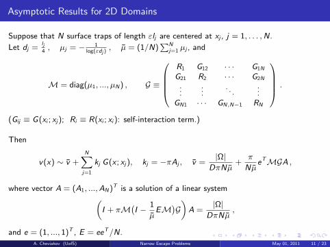
Asymptotic Results for 2D Domains
Suppose that N surface traps of length εlj are centered at xj , j = 1, . . . ,N.
Let dj =lj4, µj = − 1
log(εdj ), µ = (1/N)
∑Nj=1 µj , and
M = diag(µ1, ..., µN ) , G ≡
R1 G12 · · · G1N
G21 R2 · · · G2N
......
. . ....
GN1 · · · GN,N−1 RN
.
(Gij ≡ G(xi ; xj ); Ri ≡ R(xi ; xi ): self-interaction term.)
Then
v(x) ∼ v +N∑
j=1
kj G(x ; xj ), kj = −πAj , v =|Ω|
DπNµ+
π
NµeTMGA ,
where vector A = (A1, ...,AN )T is a solution of a linear system(I + πM
(I − 1
µEM
)G)A =
|Ω|DπNµ
,
and e = (1, ..., 1)T , E = eeT/N.
A. Cheviakov (UofS) Narrow Escape Problems May 01, 2011 11 / 23
Asymptotic Results for 2D Domains
Suppose that N surface traps of length εlj are centered at xj , j = 1, . . . ,N.
Let dj =lj4, µj = − 1
log(εdj ), µ = (1/N)
∑Nj=1 µj , and
M = diag(µ1, ..., µN ) , G ≡
R1 G12 · · · G1N
G21 R2 · · · G2N
......
. . ....
GN1 · · · GN,N−1 RN
.
(Gij ≡ G(xi ; xj ); Ri ≡ R(xi ; xi ): self-interaction term.)
Then
v(x) ∼ v +N∑
j=1
kj G(x ; xj ), kj = −πAj , v =|Ω|
DπNµ+
π
NµeTMGA ,
where vector A = (A1, ...,AN )T is a solution of a linear system(I + πM
(I − 1
µEM
)G)A =
|Ω|DπNµ
,
and e = (1, ..., 1)T , E = eeT/N.A. Cheviakov (UofS) Narrow Escape Problems May 01, 2011 11 / 23

Example: Unit Disk in 2D
Green’s function
G(x ; xi ) = − 1
πlog |x − xi |+
|x |2
4π− 1
8π, R(xi ; xi ) =
1
8π, |xi | = 1 .
Average MFPT:
v ∼ 1
DN
[− log
ε
2+
N
8− 1
N
N∑i=1
N∑j=i+1
log |xi − xj |
].
A. Cheviakov (UofS) Narrow Escape Problems May 01, 2011 12 / 23

Example: Unit Disk in 2D
As an example, in Fig. 2, the MFPT v(x) is plotted for a seven-trap configuration with a commontrap length of 2ε = 0.02.We remark that the simple result (2.14) in fact sums the infinite logarithmic expansion for the
MFPT for the special case of either exactly two arbitrarily-spaced traps or N equally-spaced trapson the boundary of the unit disk (see §2 of [12]). This result follows since, for these specialarrangements of traps, the symmetric Green’s matrix G has a cyclic matrix structure (see [12]).
x
y
−0.5 0 0.5 1
−0.8
−0.6
−0.4
−0.2
0
0.2
0.4
0.6
0.8
0
0.1
0.2
0.3
0.4
0.5
0.6
0.7
Figure 2: Surface (left figure) and contour (right figure) plots of the asymptotic MFPT (2.13),(2.14) for a unit disk with N = 7 traps of a common length 2ε = 0.02.
The minimum of the repulsive logarithmic energy term in (2.14) is evidently attained when thetraps are equally-spaced on the unit circle. For such a symmetric arrangement, and assumingwell-separated traps, a simple calculation yields (see equation (3.8) of [12])
v ∼ 1
DN
[− log
εN
2+
N
8
], v(x) ∼ v − π
DN
N∑
j=1
G(x;xj) . (2.15)
The error in this approximation is of order O(ε log ε), which is transcendentally small in comparisonto any power of −1/ log ε.
(2) The unit square
For a unit square Ω ≡ x = (x1, x2) | 0 ≤ x1, x2 ≤ 1, the explicit form of the Neumann Green’sfunction with an interior singularity was found in [20] by first calculating a Fourier series repre-sentation of the solution to (2.3), and then using certain summation formulas to extract both thelogarithmic singularity and its regular part. Upon taking the limit as the singularity ξ approachesa non-corner point of the domain boundary, one obtains a solution of the form
G(x; ξ) = − 1
πlog |x− ξ|+R(x; ξ) , (2.16)
where the regular part is given by a rapidly convergent infinite series of the explicit form
R(x; ξ) = − 1
2π
∑∞n=0 log(|1− qnz+,+||1− qnz+,−||1− qnζ+,+|)
− 1
2π
∑∞n=0 log(|1− qnζ+,−||1− qnζ−,+||1− qnζ−,−|)
− 1
2πlog
|1−z−,−|r−,−
− 1
2πlog
|1−z−,+|r−,+
+H(x1, ξ1)
− 1
2π
∑∞n=0 log(|1− qnz−,−||1− qnz−,+|) .
(2.17)
6
A. Cheviakov (UofS) Narrow Escape Problems May 01, 2011 12 / 23

Example: Unit Square in 2D
G(x ; xi ) and R(xi ; xi ) can be expressed as rapidly converging infinite sums oflogarithmic terms.
Example: Unit Square in 2D
G(x ; xi ) and R(xi ; xi ) can be expressed as rapidly converging infinite sums oflogarithmic terms.
Unit square with two traps separated by 0.5, each with a width of 2ε = 0.02.
A. Cheviakov (UofS) Narrow Escape Problems May 01, 2011 10 / 27
Unit square with two traps separated by 0.5, each with a width of 2ε = 0.02.
A. Cheviakov (UofS) Narrow Escape Problems May 01, 2011 13 / 23

3D: the Sphere
MFPT: v(x) ∼ v − |Ω|ND
∑Ni=1 Gs (x ; xi )
Green’s function:
Gs (xi ; xj ) = − 9
20π+
1
2π
(1
|xi − xj |− 1
2log[sin2
(γij
2
)+ sin
(γij
2
)]); cos(γij ) = xi ·xj
Average MFPT:
v =|Ω|
4εDN
[1 +
ε
πlog
(2
ε
)+ε
π
(−9N
5+ 2(N − 2) log 2 +
3
2+
4
NH)
+ O(ε2 log ε)].
Interaction Energy:
H(x1, . . . , xN ) =N∑
i=1
N∑j=i+1
(1
|xi − xj |− 1
2log |xi − xj | −
1
2log (2 + |xi − xj |)
)
Optimal configurations: see Matlab figures.
A. Cheviakov (UofS) Narrow Escape Problems May 01, 2011 14 / 23

Global Optimization of Trap Locations
General domain: Need to know Green’s function!
2D disk, rectangle: not too hard; involves permutations.
3D ball: 2N − 3 degrees of freedom for N traps.
A. Cheviakov (UofS) Narrow Escape Problems May 01, 2011 15 / 23

Global Optimization Software
1. The Extended Cutting Angle method (ECAM).
Deterministic global optimization technique, applicable to Lipschitz functions. (Gansolibrary).
2. Dynamical Systems Based Optimization (DSO).
A dynamical system is constructed, using a number of sampled values of the objectivefunction to introduce forces. The evolution of such a system yields a descent trajectoryconverging to lower values of the objective function. (Ganso library).
3. Lipschitz-Continuous Global Optimizer (LGO).
Commercial global optimization software, based on a combination of rigorous(theoretically convergent) global minimization strategies, as well as a number of localminimization strategies.
A. Cheviakov (UofS) Narrow Escape Problems May 01, 2011 16 / 23

Asymptotic MFPT Vs. Full Numerical Simulation
Assumptions for Asymptotic Solutions:
Small, well-separated traps.
What does it really mean?
Full numerical simulation
Finite-difference Poisson solver.
Matlab.
Variable step.
Mesh refinement to resolve traps (realistically, can compute ∼ 200× 100× 100 gridpoints).
A. Cheviakov (UofS) Narrow Escape Problems May 01, 2011 17 / 23

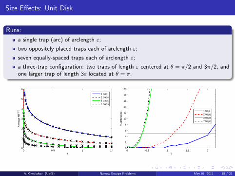
Size Effects: Unit Disk
Runs:
a single trap (arc) of arclength ε;
two oppositely placed traps each of arclength ε;
seven equally-spaced traps each of arclength ε;
a three-trap configuration: two traps of length ε centered at θ = π/2 and 3π/2, andone larger trap of length 3ε located at θ = π.
• a three-trap configuration: two traps of length ε centered at θ = π/2 and 3π/2, and one largertrap of length 3ε located at θ = π.
For the first three arrangements of traps, the result (2.14), in which ε is replaced by ε/2, determinesv(x) and v with an error that is smaller than any power of −1/ log ε. In order to obtain the samelevel of accuracy for the fourth configuration above, one must first solve the linear system (2.9) todetermine the vector A, and then calculate v(x) and v from (2.6), (2.10), and (2.13).For each of these four trap configurations, it was found that the asymptotic and numerical results
for the average MFPT v are within 1% agreement when the length of the traps is of the order ofone. A sample comparative contour plot of v(x) for the 3-trap configuration (Fig. 3) shows a closeagreement between the asymptotic and numerical results for the MFPT everywhere in the domainexcept for a very small region near the traps.
x1
x 2
Asymptotic MFPT v(x)
−1 −0.5 0 0.5 1
−0.8
−0.6
−0.4
−0.2
0
0.2
0.4
0.6
0.8
0.2
0.4
0.6
0.8
1
1.2
1.4
x1
x 2Numerical MFPT v(x)
−1 −0.5 0 0.5 1
−0.8
−0.6
−0.4
−0.2
0
0.2
0.4
0.6
0.8
0.2
0.4
0.6
0.8
1
1.2
1.4
−1 −0.5 0 0.5 10
0.2
0.4
0.6
0.8
1
1.2
1.4
Comparison along x1=0
x
v(x)
AsymptoticNumerical
Figure 3: Comparison of asymptotic (left figure) and numerical (middle figure) predictions for the MFPTv(x) for a three-trap configuration in the unit disk, with two traps of length ε (centered at θ = π/2 andθ = 3π/2), and one trap of length 3ε (centered at θ = π). Here ε = 0.06. Right figure: comparison ofasymptotics and numerics along the cross-section x1 = 0.
The results for the disk are summarized in Fig. 4, where the average MFPT v is plotted as afunction of ε for the one-, two-, three- and seven-trap configurations. In particular, for one trap,the results are within 5% agreement for a trap length ε . 2, which is roughly 1/3 of the lengthof the domain boundary. Similarly, for for seven equally-spaced traps, the results are within 5%agreement for a trap length ε . 0.35, which is roughly 40% of the length of the domain boundary.
0 0.5 1 1.50
1
2
3
4
5
6
ε
Ave
rage
MF
PT
1 trap2 traps3 traps7 traps
0 0.5 1 1.5 20
2
4
6
8
10
12
14
16
18
20
ε
% d
iffer
ence
1 trap2 traps3 traps7 traps
Figure 4: Left figure: Dependence of the average MFPT v on the trap length ε for one-, two-, three-, andseven-trap configurations in a unit disk. The curves are the asymptotic formulas, and the crosses are fullnumerical results. Right figure: percent difference between asymptotic and numerical results versus ε.
10
A. Cheviakov (UofS) Narrow Escape Problems May 01, 2011 18 / 23
Size Effects: Unit Disk
Runs:
a single trap (arc) of arclength ε;
two oppositely placed traps each of arclength ε;
seven equally-spaced traps each of arclength ε;
a three-trap configuration: two traps of length ε centered at θ = π/2 and 3π/2, andone larger trap of length 3ε located at θ = π.
• a three-trap configuration: two traps of length ε centered at θ = π/2 and 3π/2, and one largertrap of length 3ε located at θ = π.
For the first three arrangements of traps, the result (2.14), in which ε is replaced by ε/2, determinesv(x) and v with an error that is smaller than any power of −1/ log ε. In order to obtain the samelevel of accuracy for the fourth configuration above, one must first solve the linear system (2.9) todetermine the vector A, and then calculate v(x) and v from (2.6), (2.10), and (2.13).For each of these four trap configurations, it was found that the asymptotic and numerical results
for the average MFPT v are within 1% agreement when the length of the traps is of the order ofone. A sample comparative contour plot of v(x) for the 3-trap configuration (Fig. 3) shows a closeagreement between the asymptotic and numerical results for the MFPT everywhere in the domainexcept for a very small region near the traps.
x1
x 2
Asymptotic MFPT v(x)
−1 −0.5 0 0.5 1
−0.8
−0.6
−0.4
−0.2
0
0.2
0.4
0.6
0.8
0.2
0.4
0.6
0.8
1
1.2
1.4
x1
x 2
Numerical MFPT v(x)
−1 −0.5 0 0.5 1
−0.8
−0.6
−0.4
−0.2
0
0.2
0.4
0.6
0.8
0.2
0.4
0.6
0.8
1
1.2
1.4
−1 −0.5 0 0.5 10
0.2
0.4
0.6
0.8
1
1.2
1.4
Comparison along x1=0
x
v(x)
AsymptoticNumerical
Figure 3: Comparison of asymptotic (left figure) and numerical (middle figure) predictions for the MFPTv(x) for a three-trap configuration in the unit disk, with two traps of length ε (centered at θ = π/2 andθ = 3π/2), and one trap of length 3ε (centered at θ = π). Here ε = 0.06. Right figure: comparison ofasymptotics and numerics along the cross-section x1 = 0.
The results for the disk are summarized in Fig. 4, where the average MFPT v is plotted as afunction of ε for the one-, two-, three- and seven-trap configurations. In particular, for one trap,the results are within 5% agreement for a trap length ε . 2, which is roughly 1/3 of the lengthof the domain boundary. Similarly, for for seven equally-spaced traps, the results are within 5%agreement for a trap length ε . 0.35, which is roughly 40% of the length of the domain boundary.
0 0.5 1 1.50
1
2
3
4
5
6
ε
Ave
rage
MF
PT
1 trap2 traps3 traps7 traps
0 0.5 1 1.5 20
2
4
6
8
10
12
14
16
18
20
ε
% d
iffer
ence
1 trap2 traps3 traps7 traps
Figure 4: Left figure: Dependence of the average MFPT v on the trap length ε for one-, two-, three-, andseven-trap configurations in a unit disk. The curves are the asymptotic formulas, and the crosses are fullnumerical results. Right figure: percent difference between asymptotic and numerical results versus ε.
10
A. Cheviakov (UofS) Narrow Escape Problems May 01, 2011 18 / 23
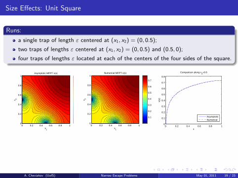
Size Effects: Unit Square
Runs:
a single trap of length ε centered at (x1, x2) = (0, 0.5);
two traps of lengths ε centered at (x1, x2) = (0, 0.5) and (0.5, 0);
four traps of lengths ε located at each of the centers of the four sides of the square.
(2) The unit square
For the unit square, the following four trap configurations were considered:
• a single trap of length ε centered at (x1, x2) = (0, 0.5);
• two traps of lengths ε centered at (x1, x2) = (0, 0.5) and (0.5, 0);
• four traps of lengths ε located at each of the centers of the four sides of the square.
The asymptotic MFPT v(x) and the asymptotic average MFPT v were computed from (2.6), (2.16),and (2.17).A comparative plot of the MFPT v(x) for the case of two traps of a common length ε = 0.03 is
given in Fig. 5, while the comparisons of the average MFPT v for all three trap configurations aresummarized in Fig. 6. Compared to the situation for the unit disk, the asymptotic results for v andv for the square domain reliably predict the full numerical values for a slightly smaller range of ε.For example, for one trap, the 1% agreement between the asymptotic and the numerical solution isonly observed for ε . 0.2 (ε . 0.4 for 5% agreement). For the 4-trap case, we have 1% agreementwhen ε . 0.1 (10% trap surface area fraction), and 5% agreement when ε . 0.25 (25% trap surfacearea fraction). These results show that one can still reliably use the asymptotic theory at ratherlarge values of the small parameter ε. The slightly smaller range of validity in ε in comparisonto the case of the unit disk can probably be attributed to the effects of the non-smooth domainboundary of the square.
x1
x 2
Asymptotic MFPT v(x)
0 0.2 0.4 0.6 0.8 10
0.2
0.4
0.6
0.8
1
0
0.1
0.2
0.3
0.4
0.5
0.6
0.7
x1
x 2
Numerical MFPT v(x)
0 0.2 0.4 0.6 0.8 10
0.2
0.4
0.6
0.8
1
0.1
0.2
0.3
0.4
0.5
0.6
0.7
0 0.2 0.4 0.6 0.8 10
0.1
0.2
0.3
0.4
0.5
0.6
0.7
0.8
Comparison along x2=0.5
x
v(x)
AsymptoticNumerical
Figure 5: Comparison of the asymptotic (left figure) and numerical (middle figure) results for the MFPTv(x) for two traps of a common length ε = 0.03 for the unit square. Right figure: comparison of asymptoticand numerical results along the cross-section x2 = 0.5.
11
A. Cheviakov (UofS) Narrow Escape Problems May 01, 2011 19 / 23

Size Effects: Unit Square
Runs:
a single trap of length ε centered at (x1, x2) = (0, 0.5);
two traps of lengths ε centered at (x1, x2) = (0, 0.5) and (0.5, 0);
four traps of lengths ε located at each of the centers of the four sides of the square.
0 0.1 0.2 0.3 0.4 0.50
0.5
1
1.5
2
2.5
ε
Ave
rage
MF
PT
1 trap2 traps4 traps
0 0.1 0.2 0.3 0.4 0.50
1
2
3
4
5
6
7
8
9
10
ε
% d
iffer
ence
1 trap2 traps4 traps
Figure 6: Left figure: Dependence of the average MFPT v on the trap length ε for one-, two-, and four-trapconfigurations in a unit square. The curves correspond to the asymptotic results, and the crosses are the fullnumerical results. Right figure: percent difference between asymptotic and numerical results.
(3) The unit sphere
For the unit sphere, we consider the simplest configurations of one, two, and three, equally-spacedcircular traps of radius ε centered on the equator of the unit sphere. A sample comparative contourplot of the MFPT v(x) in the equatorial cross-section of the sphere for a single trap of radiusε = 0.2, a = 1, is shown in Fig. 7. As seen from Fig. 8, the 1% agreement between the asymptoticand the numerical results for the average MFPT v for a single trap is attained for trap radii withε . 0.8, which corresponds to a 16% trap surface area fraction.
y
x
Asymptotic MFPT at z=0
0.5 0 0.51
0.8
0.6
0.4
0.2
0
0.2
0.4
0.6
0.8
1
0 1 2 3 4 5
y
x
Numerical MFPT at z=0
0.5 0 0.51
0.8
0.6
0.4
0.2
0
0.2
0.4
0.6
0.8
1
1 2 3 4 5 6
1 0.5 0 0.5 10
1
2
3
4
5
6
7
Comparison along x2=x
3=0
x
v(x
)
Asymptotic
Numerical
Figure 7: Comparison of asymptotic (left figure) and numerical (middle figure) results for the MFPT v(x)for one trap of radius ε = 0.2, on the boundary of the unit sphere. Right figure: comparison of asymptoticand numerical results along the line x2 = x3 = 0
3.2 Trap Separation Effects
The results (2.10) and (2.22) for the average MFPT in a general 2-D and a spherical 3-D domain,respectively, are valid under the assumption of “well-separated” boundary traps. To study how theasymptotic results perform when the traps are not necessarily so well-separated, we compare theasymptotic and full numerical results for the whole range of two-trap configurations, ranging fromtwo touching traps to the maximal possible separation distance in each given configuration.The following comparisons suggest that for the domains considered below, the asymptotic formulas
for the average MFPT are still rather reliable, in the sense of being within 1% of the full numericalresult, even for small separation distances of order O(ε).
12
A. Cheviakov (UofS) Narrow Escape Problems May 01, 2011 19 / 23
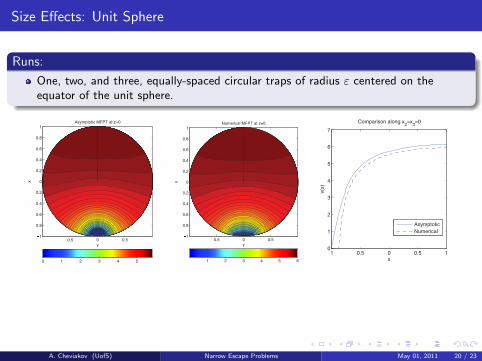
Size Effects: Unit Sphere
Runs:
One, two, and three, equally-spaced circular traps of radius ε centered on theequator of the unit sphere.
0 0.1 0.2 0.3 0.4 0.50
0.5
1
1.5
2
2.5
ε
Ave
rage
MF
PT
1 trap2 traps4 traps
0 0.1 0.2 0.3 0.4 0.50
1
2
3
4
5
6
7
8
9
10
ε
% d
iffer
ence
1 trap2 traps4 traps
Figure 6: Left figure: Dependence of the average MFPT v on the trap length ε for one-, two-, and four-trapconfigurations in a unit square. The curves correspond to the asymptotic results, and the crosses are the fullnumerical results. Right figure: percent difference between asymptotic and numerical results.
(3) The unit sphere
For the unit sphere, we consider the simplest configurations of one, two, and three, equally-spacedcircular traps of radius ε centered on the equator of the unit sphere. A sample comparative contourplot of the MFPT v(x) in the equatorial cross-section of the sphere for a single trap of radiusε = 0.2, a = 1, is shown in Fig. 7. As seen from Fig. 8, the 1% agreement between the asymptoticand the numerical results for the average MFPT v for a single trap is attained for trap radii withε . 0.8, which corresponds to a 16% trap surface area fraction.
y
x
Asymptotic MFPT at z=0
0.5 0 0.51
0.8
0.6
0.4
0.2
0
0.2
0.4
0.6
0.8
1
0 1 2 3 4 5
y
x
Numerical MFPT at z=0
0.5 0 0.51
0.8
0.6
0.4
0.2
0
0.2
0.4
0.6
0.8
1
1 2 3 4 5 6
1 0.5 0 0.5 10
1
2
3
4
5
6
7
Comparison along x2=x
3=0
x
v(x
)
Asymptotic
Numerical
Figure 7: Comparison of asymptotic (left figure) and numerical (middle figure) results for the MFPT v(x)for one trap of radius ε = 0.2, on the boundary of the unit sphere. Right figure: comparison of asymptoticand numerical results along the line x2 = x3 = 0
3.2 Trap Separation Effects
The results (2.10) and (2.22) for the average MFPT in a general 2-D and a spherical 3-D domain,respectively, are valid under the assumption of “well-separated” boundary traps. To study how theasymptotic results perform when the traps are not necessarily so well-separated, we compare theasymptotic and full numerical results for the whole range of two-trap configurations, ranging fromtwo touching traps to the maximal possible separation distance in each given configuration.The following comparisons suggest that for the domains considered below, the asymptotic formulas
for the average MFPT are still rather reliable, in the sense of being within 1% of the full numericalresult, even for small separation distances of order O(ε).
12
A. Cheviakov (UofS) Narrow Escape Problems May 01, 2011 20 / 23
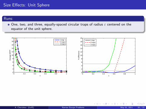
Size Effects: Unit Sphere
Runs:
One, two, and three, equally-spaced circular traps of radius ε centered on theequator of the unit sphere.
0 0.2 0.4 0.6 0.8 10
2
4
6
8
10
12
14
16
18
20
ε
Ave
rage
MF
PT
1 trap2 traps3 traps
0 0.2 0.4 0.6 0.8 10
2
4
6
8
10
12
14
16
18
20
ε%
diff
eren
ce
1 trap2 traps3 traps
Figure 8: Left figure: Dependence of the average MFPT v on the common trap radius ε for one, two, andthree traps that are equally-spaced on the equator of the unit sphere. The curves correspond to the asymp-totic results, and the crosses to full numerical results. Right figure: percent difference between asymptoticand numerical results.
(1) The unit square
For the unit square, two configurations were considered. In the first configuration, two identicaltraps of length ε were located on adjacent sides, centered at a point at a distance L from the corner(ε/2 ≤ L ≤ 1−ε/2, see Fig. 5). In the second configuration, two identical traps were symmetricallylocated on one side of the square, at a distance L between their centers (ε ≤ L ≤ 1− ε).For traps of length ε = 0.05, a plot of the numerical and asymptotic average MFPT and their
relative difference is shown in Fig. 9. For traps located on one side of the square the agreementbetween the asymptotic and numerical results is within 1% for all values of L. For traps locatedon adjacent sides of the square, the asymptotic result overshoots by approximately 6% when thetraps are touching at the origin, but is within approximately 2% of the full numerical results wheneach trap is centered at a distance 0.05 from the origin.
0.1 0.2 0.3 0.4 0.5 0.6 0.7 0.8 0.90.4
0.6
0.8
1
1.2
1.4
1.6
1.8
2
Distance from the corner (i) / between traps (ii)
Ave
rage
MF
PT
(i) two traps (adjacent sides)(ii) two traps (one side)
0.1 0.2 0.3 0.4 0.5 0.6 0.7 0.8 0.90
1
2
3
4
5
6
7
Distance between trap centers
% d
iffer
ence
(i) two traps (adjacent sides)(ii) two traps (one side)
Figure 9: Left figure: Effect of trap separation in the unit square: comparison of the asymptotic andnumerical results for the average MFPT v for two traps of sizes ε = 0.05. The percent difference is shownin the right figure. (i) Average MFPT for two traps located on adjacent sides, as a function of the distancefrom the corner. (ii) Average MFPT for two traps located symmetrically on one side, as a function of thedistance between traps.
(2) The unit sphere and the unit disk.
As shown in Fig. 10, a very good agreement between the asymptotic and numerical results forthe average MFPT is also observed for the case of two arbitrarily-spaced traps on the surface of
13
A. Cheviakov (UofS) Narrow Escape Problems May 01, 2011 20 / 23

Separation Effects
Runs:
Unit square: two identical traps on adjacent sides.
Unit square: two identical traps on same side.
Unit disk: two identical traps.
Unit sphere: two identical traps on equator.
0 0.2 0.4 0.6 0.8 10
2
4
6
8
10
12
14
16
18
20
ε
Ave
rage
MF
PT
1 trap2 traps3 traps
0 0.2 0.4 0.6 0.8 10
2
4
6
8
10
12
14
16
18
20
ε
% d
iffer
ence
1 trap2 traps3 traps
Figure 8: Left figure: Dependence of the average MFPT v on the common trap radius ε for one, two, andthree traps that are equally-spaced on the equator of the unit sphere. The curves correspond to the asymp-totic results, and the crosses to full numerical results. Right figure: percent difference between asymptoticand numerical results.
(1) The unit square
For the unit square, two configurations were considered. In the first configuration, two identicaltraps of length ε were located on adjacent sides, centered at a point at a distance L from the corner(ε/2 ≤ L ≤ 1−ε/2, see Fig. 5). In the second configuration, two identical traps were symmetricallylocated on one side of the square, at a distance L between their centers (ε ≤ L ≤ 1− ε).For traps of length ε = 0.05, a plot of the numerical and asymptotic average MFPT and their
relative difference is shown in Fig. 9. For traps located on one side of the square the agreementbetween the asymptotic and numerical results is within 1% for all values of L. For traps locatedon adjacent sides of the square, the asymptotic result overshoots by approximately 6% when thetraps are touching at the origin, but is within approximately 2% of the full numerical results wheneach trap is centered at a distance 0.05 from the origin.
0.1 0.2 0.3 0.4 0.5 0.6 0.7 0.8 0.90.4
0.6
0.8
1
1.2
1.4
1.6
1.8
2
Distance from the corner (i) / between traps (ii)
Ave
rage
MF
PT
(i) two traps (adjacent sides)(ii) two traps (one side)
0.1 0.2 0.3 0.4 0.5 0.6 0.7 0.8 0.90
1
2
3
4
5
6
7
Distance between trap centers
% d
iffer
ence
(i) two traps (adjacent sides)(ii) two traps (one side)
Figure 9: Left figure: Effect of trap separation in the unit square: comparison of the asymptotic andnumerical results for the average MFPT v for two traps of sizes ε = 0.05. The percent difference is shownin the right figure. (i) Average MFPT for two traps located on adjacent sides, as a function of the distancefrom the corner. (ii) Average MFPT for two traps located symmetrically on one side, as a function of thedistance between traps.
(2) The unit sphere and the unit disk.
As shown in Fig. 10, a very good agreement between the asymptotic and numerical results forthe average MFPT is also observed for the case of two arbitrarily-spaced traps on the surface of
13
Unit square
A. Cheviakov (UofS) Narrow Escape Problems May 01, 2011 21 / 23

Separation Effects
Runs:
Unit square: two identical traps on adjacent sides.
Unit square: two identical traps on same side.
Unit disk: two identical traps.
Unit sphere: two identical traps on equator.
the unit disk or unit sphere. For the unit disk, traps of arclength ε = 0.05 were chosen. For theunit sphere, we chose circular traps of radius ε = 0.2 located on the equator. For all separationdistances, ranging from touching traps to traps on opposite sides of a diameter, the discrepancybetween the asymptotic and numerical results is well within 1% for both domains.
0.5 1 1.5 2 2.5 31.5
2
2.5
3
3.5
4
Distance between trap centers
Ave
rage
MF
PT
(i) disk(ii) sphere
0.5 1 1.5 2 2.5 30
0.5
1
1.5
Distance between trap centers
% d
iffer
ence
(i) disk(ii) sphere
Figure 10: Left figure: Effect of trap separation in the unit disk (i) and the unit sphere (ii). Comparison ofasymptotic and numerical results for the MFPT v. Unit disk: two traps of arclength ε = 0.05. Unit sphere:two circular traps of radius ε = 0.2 located on the equator. The right figure shows the percent differencebetween the asymptotic and numerical results.
4 Optimal Location of Traps on the Unit Sphere
We now determine the optimal arrangements of N traps on the boundary of a given domain Ω thatminimize the average MFPT v. In [12,13], it was shown that such optimal trap arrangements alsomaximize the principal eigenvalue of the Laplacian in the corresponding domain with traps, thusmaximizing the diffusion rate from a domain with small holes on an otherwise reflecting boundary.Here the attention is restricted to the sphere, which is a fundamental domain both from the pointof view of applications and the complexity of numerical optimization. Indeed, boundary trapson the surface of two-dimensional domains correspond physically to slit-like holes extended in theinvariant direction on the surface of three-dimensional cylinders. Location optimization for suchtraps can involve permutations, but is otherwise much simpler than that for a sphere.Consider N traps located on a unit sphere. In order to optimize the average MFPT v in (2.22),
one has to find coordinates of N repelling particles on the sphere, which correspond to the globalminimum of the interaction term pc(x1, . . . , xN ) in (2.22). One thus has a global optimizationproblem for a function of 2N variables (e.g., spherical angles).Many global optimization techniques have recently been developed, including methods for non-
smooth optimization, optimization in bounded and unbounded domains, and optimization subjectto constraints. For low-dimensional problems, exact methods are available, whereas for higher-dimensional problems one is usually restricted to using partly heuristic numerical optimizationalgorithms. For a review of continuous global optimization algorithms and software, see [21,22].For the computations below, the dynamical systems-based optimization method (DSO), and the
extended cutting angle method (ECAM) from the open software library GANSO [23], were used.These algorithms proved to be stable and sufficiently fast for not-very-large numbers of traps(N . 25).
4.1 N Identical Traps
For N traps of a common radius ε on the unit sphere, it is convenient to use spherical coordinatesxj = (1, θj , φj), for j = 1, . . . , N , where θj is the azimuthal angle, and φj is the polar angle.
14
Unit disk and sphere
A. Cheviakov (UofS) Narrow Escape Problems May 01, 2011 21 / 23

Conclusions and Open Problems
Conclusions
A general formula for MFPT and average MFPT for 2D and 3D domains ispresented.
Formula can be used directly when Neumann Green’s function is known.
Highest-order term involves interaction, allows for global optimization.
Asymptotic formulas are applicable for substantially large traps and small separationdistances.
Open problems
Fast-multipole methods can be used to compute Neumann Green’s function for anarbitrary 3-D domain with smooth boundary. These can be combined withasymptotic formulas.
Compare with results following from dilute trap fraction limit of homogenizationtheory, as N →∞.
A. Cheviakov (UofS) Narrow Escape Problems May 01, 2011 22 / 23

Some references
B. Bergersen, D. Boal, P. Palffy-Muhoray,
Equilibrium Configurations of Particles on the Sphere: The Case of Logarithmic Interactions, J. Phys. A:Math Gen., 27, No. 7, (1994), pp. 2579–2586.
S. Pillay, M. J. Ward, A. Peirce, T. Kolokolnikov,
An Asymptotic Analysis of the Mean First Passage time for Narrow Escape Problems: Part I:Two-Dimensional Domains, Multiscale Model. Simul., 8, No. 3, (2010), pp. 803–835.
A. F. Cheviakov, M. J. Ward, R. Straube,
An Asymptotic Analysis of the Mean First Passage Time for Narrow Escape Problems: Part II: theSphere. Multiscale Model. Simul. 8(3), (2010), 836–870.
GANSO Software Library: University of Ballarat, Ballarat, Victoria, Australia.
www.ballarat.edu.au/ciao
J. D. Pinter,
Global Optimization in Action, Kluwer Academic Publishers, Dordrecht, Netherlands, (1996).
M. J. Ward, J. B. Keller,
Strong Localized Perturbations of Eigenvalue Problems, SIAM J. Appl. Math. 53, No. 3, (1993),pp. 770–798.
A. Cheviakov (UofS) Narrow Escape Problems May 01, 2011 23 / 23