1

Mathematical Evaluation of Body Cooling

Using the Heat Equation

BENG221

Oct 24th, 2014

Christopher Chu

Clement Lee

Joshua Wei

Alexander Williams

2

Introduction

Thermoregulation is one of the body’s many homeostatic processes. It is necessary

because most proteins function only in a narrow temperature range. If thermoregulation fails,

critical body functions can shut down as proteins denature. Primary methods of thermoregulation

include sweating and vasodilation to decrease core body temperature, and vasoconstriction and

shivering to increase temperature. In general this scheme of heating and cooling is effective at

maintaining a core body temperature of 37°C. Additionally, the human body has adapted to

many different environments be it through cultural adaptations or physiological changes.

In extreme conditions, sweating is the most effective methods of heat extraction since the

evaporation of water requires a large amount of energy, but vasodilation still remains an

effective method for cooling as long as external temperature is less than core body temperature.

Dense beds of specialized vessels called arteriovenous anastomoses exist in different locations

among species which facilitate heat transfer. Arteriovenous anastomoses bypass capillaries

which shunt blood flow, allowing for large volumes of blood to pass through the surfaces of the

body containing them. These regions may be thought of as “radiators” of heat[3]. In humans,

these beds primarily lie in the hands, feet, and face. Vasodilation and vasoconstriction control the

flow of blood to the arteriovenous anastomoses, adjusting both the volume of blood exposed to

external temperatures, and the surface area over which heat exchange can occur.

One way to aid the process of changing body temperature is by changing the local

temperature in regions where blood flow is significant, such as the radiator surfaces. Hospitals

often achieve this by applying cold compresses to the pulse points on the body, such as the neck,

elbows, and wrist[4]. Another method that has been gaining momentum is using heating or

cooling ‘gloves’ that not only change the temperature near the hand, but also apply a slight

vacuum to decrease pressure on the tissue and force local vasodilation. A company called

AVAcore uses this vacuum supplemented perfusion to help return athletes’ core body

temperature and heart rate to basal levels more quickly after exercise, allowing for extended

periods of physical exertion and optimal performance in extreme conditions and reduced

fatigue[5]. The technology has also been tested on military personnel and industrial workers with

similar results[6].

Problem Statement

Heat transferred from our skin into the atmosphere is released through radiation, a rather

ineffective and slow method of transport. Typically, cold objects are applied directly to the skin

so convection, a much faster process, can transfer heat away from the body. AVAcore claims

that the application of cold objects to the skin do not sufficiently facilitate heat transfer since

cold temperatures cause vasoconstriction, decreasing the radiative abilities of arteriovenous

anastomoses. The company also claims conventional methods are ineffective because the

treatments have difficulty penetrating the body's insulating layers of tissue to facilitate heat

transfer. In our model, we examine the claim that AVAcore’s device with the vacuum increased

perfusion is necessary to facilitate sufficient heat transfer and subsequent cooling, or whether

conventional methods can bring core body temperature down to normal from an elevated

temperature in a reasonable and comparable amount of time.

3

In this report we model heat flow in arm under various body temperature conditions to

simulate cases of exercise and rest. We perform these studies in the context of patients holding

their hands against a cool object such as a peltier plate, a metal plate being cooled by water bath,

or simply cold water at a constant, controllable temperature. We obtain temperature profiles over

the length of the arm by solving the heat equation. Finally, we calculate total heat dissipated

under various situations to quantitatively compare between our simulation conditions.

Assumptions and their Consequences

Our assumptions are as follows (Refer to figure 1 in next section):

1) The arm is a single, homogeneous tissue. However, some properties bone, muscle, fat,

blood, and skin are all incorporated into the model partially via the constants used for

simulation. Furthermore, all components of the homogeneous tissue are static. Hence we

do not account for blood flow in our model.

2) We assume no radial heat transfer. Rather, heat may only travel down the axis of the arm

from body to hand, which we denote as the x-axis. Consequently, our problem is a 1D

heat transfer problem.

3) The only heat exchange of the arm with its “surroundings” are with the rest of the body,

which we denote x=0, and with the cooling object at the hand, which we denote x=L.

Furthermore, the exchange is instantaneous, allowing for value boundary conditions at

both x=0 and x=L. In particular, the temperature at the beginning of the arm (x=0) is

equal to the core body temperature. Similarly, the temperature at the hand (x=L) is equal

to the temperature of the cooling object.

4) As previously stated, we consider a state of constant exercise. This, along with

assumption 3, means that the core body temperature does not fall, despite cooling or heat

dissipation from the hand. Rather, it stays at an elevated body temperature throughout the

time we consider.

5) We disregard the possibility of metabolic heat production, assuming that the change in

the temperature distribution of the arm from the initial condition is caused by the

temperature gradient from the body to the hand.

Mathematical Expression and Analytical Solution

Fig. 1: Spatial definitions of coordinates along the length of the arm

4

Governing Equation

With our assumptions in mind, we mathematically model our problem using the heat

equation. The most general statement of this problem in cylindrical coordinates is

By assumption 2, the first and second terms of the right hand side of the equation are neglected.

That is, we say that the temperature is not dependent on r or Φ, and so their derivatives become

zero.

Similarly, the generation term, Q, becomes 0 by assumption 5. Note in the following equation

that we have changed the variable z to x for convenience, as our problem has now become a 1-

dimensional problem.

Note also in the equation above that we have divided both sides of the equation by ρc, which

gives the constant

where c is the heat capacity of the tissue, k is the thermal conductivity of the tissue, and ρ is the

tissue’s mass density. D is the thermal diffusivity.

At last we are left with the 1D heat equation with no generation term.

This heat equation was analyzed to determine the temperature distribution over the length of the

arm over a given time.

Boundary and Initial Conditions

In accordance with figure 1 and our problem conditions stated in the assumptions, the

boundary and initial conditions were defined as follows:

where the temperature at start of the arm is assumed to be equivalent to elevated core body

temperature 𝑇𝑜; the end of the arm at the device hand is assumed to be the temperature of the

cooling plate, 𝑇𝐿; and the arm is assumed to initially be some temperature 𝑇𝑏 for all x. These

follow from assumptions 3 and 4.

Analytical Solution

Addressing Inhomogeneity

The boundary conditions are nonhomogeneous. This precludes direct use of separation of

variables to solve the PDE. Instead, the general solution will be the sum of a “homogeneous” and

“particular” solution as follows:

5

where 𝑣ℎ is the homogeneous solution and 𝑇𝑝 is the particular solution.

Particular Equilibrium Solution

The particular solution accounts for the boundary condition inhomogeneity. It is akin to

finding a steady state or equilibrium temperature distribution. Hence ∂T/∂t=0, and the equation

reduces simply to the following equation

The boundary conditions remain as stated for the overall problem. We ignore the initial condition

in the steady state calculation. This is a simple second order ODE. Integrating twice yields the

linear solution

Applying the boundary conditions, the coefficients A and B can be determined as follows.

The final equilibrium temperature distribution is

Homogenous Problem - Displacement from Equilibrium and Separation of Variables

We now solve the homogeneous problem for v(x,t). v(x,t) is the temperature

displacement from the equilibrium temperature.

The boundary conditions must be expressed for the displacement v(x,t). They may be found by

substitution.

For the displacement v(x,t), the boundary conditions are homogeneous and linear. In order to use

separation of variables, the equation itself must also be homogeneous and linear. Because

∂T/∂t=∂v/∂t and ∂2T/∂t

2=∂

2v/∂t

2 (since the equilibrium solution is only a function of x), v(x,t)

must also satisfy the heat equation as previously stated.

This is a linear homogeneous PDE. Therefore we can use separation of variables to solve it. We

assume that the form of the solution is of the product form

Taking the first and second derivatives of v(x,t) with respect to time and space respectively,

substituting them into the PDE, and finally dividing both sides by G(t) and Φ(x) separates the

variables and shown below.

6

Note that we also rearranged the constants for convenience. Because G is a function only of t and

Φ is only a function of x, the only way the derivative expressions above may be equal is if both

expressions equal some constant. We select -λ for convenience in finding the eigenvalues.

Spatial Component

The spatial component is shown to be a second order ODE:

To find nontrivial solutions, cases must be considered based on the value of 𝜆, the eigenvalue.

Case 1

𝜆 = 0

boundary conditions are applied, and a trivial solution is obtained.

𝛷(0) = 0 = 𝐴(0) + 𝐵 B = 0

𝛷(𝐿) = 0 = 𝐴(𝐿) + 𝐵

𝐴 = 0

Case 2

𝜆 < 0

By applying boundary conditions, another trivial solution is obtained.

𝛷(0) = 0 = 𝐶1 + 𝐶2 𝐶1 = − 𝐶2

𝛷(0) = 0 = 𝐶1𝑒𝐿√|𝜆| + 𝐶2𝑒−𝐿√|𝜆|

0 = 𝐶1(𝑒𝐿√|𝜆| − 𝐶2𝑒−𝐿√|𝜆| )

𝐶1 = 𝐶2 = 0

7

Case 3

𝜆 > 0

The solution, along with the Euler expansion, is as follows:

Boundary conditions are applied:

𝛷(0) = 0 = 𝐶1𝑐𝑜𝑠(0√𝜆) + 𝐶2𝑠𝑖𝑛(0√𝜆)

𝛷(0) = 0 = 𝐶1𝑐𝑜𝑠(𝐿√𝜆) + 𝐶2𝑠𝑖𝑛(𝐿√𝜆)

In order to satisfy the relationship while maintaining non-triviality, 𝐶2cannot equal zero;

therefore, 𝜆 must be some value which allows the sine expression to equal zero.

for n = 1,2,3...

The corresponding spatial component of the solution is then

for n = 1,2,3...

Temporal Component

Analysis of temporal component by separation of variables shows that the solution G(t) is

an exponential expression

Determining Constant Term

Multiplying the temporal and spatial components provides the general solution for the

displacement v(x,t):

Now the initial condition is used to determine constant 𝐴𝐴. As with the boundary conditions, we

must determine the initial condition for v(x,t) from the initial condition for T(x,t). This new

8

initial condition is simply the the initial condition of T(x,t) minus the the steady state temperature

solution. With this knowledge, we now substitute t=0 and obtain the following expression for

solving the constant An.

Next we multiply both sides by sin(nπx/L) and integrate both sides of the equation over the

domain of the problem x = [0,L].

In the above expression we applied the orthogonality of the sine function to obtain the right most

expression. Proceeding, we solve for the constant by substituting the initial condition for T(x,t)

and the equilibrium temperature distribution.

To solve this integral, we must integrate by parts.

Finally, the final analytical solution for the original heat equation is

where An is given by the above expression Am.

Temperature Profiles - Analytical and Numerical Solutions

Constant values that define D must be determined in order to plot the analytical solution.

The values used are presented in Table 1 and are based on previously established values from

literature.

9

Table 1. Table of Constants

Specific heat capacity[7], thermal conductivity[8], and mass density[9] are estimated based on a

combination of published values for different tissue types. In particular, we found specific heats,

thermal conductivities, and mass densities for different components of the arm, including bone,

fat, skin, blood, and muscle, and took average values of the individual quantities as our constants

for simulation. Our boundary conditions and initial condition vary for different scenarios we

present below, so we refrain from setting specific values here. However, we explain now a few

important temperatures that we used and explain their significance. The boundary condition of

core body temperature equal to 39°C represents an extreme physiological limit. A person who is

feverish should not reach this temperature. However, this number would not be unusual for an

individual under great physical exertion, such as a soldier in a desert environment, a firefighter at

the scene of the fire, or an athlete in play. The hand temperature of 15°C could be achieved when

the hand is in contact with a cooling object. The initial condition, Tb, is selected to be equal to

the core body temperature (Tb=To).

Analytical Solutions

Plots are made with different numbers of terms (2, 10, and 1000) from the analytical

solution using the same boundary and initial conditions. The MATLAB code used to generate

these are in Appendix A. The boundary and initial conditions for the solutions shown in figures

2-4 are Tb=To=39°C and TL=15°C. Analytical solutions were also generated for the boundary

and initial conditions to be described in figures 5-6 and 8, but they are not shown. They are

discussed briefly in the discussion section. For the axes in all figures 2-14, the units are seconds

for time, cm for x, and °C for T(x,t) (denoted u(x,t) in the plots).

Fig. 2. Surf plot of first 2 terms from two different angles

10

Fig. 3. Surf plot of first 10 terms from two different angles

Fig. 4. Surf plot of first 1000 terms from two different angles

Numerical Solution

MATLAB’s built in pdepe is used to generate the surf plots in this section (Appendix B).

Different scenarios are examined by altering the problem’s boundary conditions. The total heat

dissipated is also analyzed in each case to further study the effectiveness of the cooling in the

arm simply by holding a cold object.

Since pdepe computes the solution at every length interval of dx along the arm for a

given time interval, we can use the trapezoidal rule to approximate the integral of the

temperature distribution at a particular time point and hence calculate the heat dissipated.

We take the average temperature between every interval and subtract from initial temp. This is

multiplied by the length interval, the heat capacity of the tissue, tissue density and the cross

sectional area of the arm (Table 1). The arm radius was approximated as 5 cm to account for a

bulkier athlete, who would be a likely candidate for using a cooling device

11

Fig. 5. This first case models the hand

temperature profile at a basal condition

assuming normal body temperature

(To=37°C) and room temperature

surroundings (TL=25° C). A cooling

device is not considered for this

situation. Using our integration scheme,

we determine the total heat dissipated

at some final time. Here, we

consistently set this value at t=10,000 s

~ 3hrs, to exaggerate the value. Given

these conditions, Q_lost = 2.2182e4 J

at t=10,000s. Also, the theoretical total

heat in the arm initially for the core

body temperature of TL=To=37°C is

Qto=6.9390e5 J. The value used for this

theoretical total changes in the following cases to match the initial condition used. This is

basically the amount of heat in the arm at initial condition. It is calculated simply by multiplying

the value of the initial condition by the full length of the arm L and then multiplying by the heat

capacity of the tissue, tissue density and the cross sectional area of the arm.

Fig. 6 (Middle). To verify the usefulness of our model, we next examined an irregular case

where the body is at a near hypothermic temperature of To=34°C and examined the temperature

profile. Qlost=1.6636e4 J, which is reasonable considering the body is cooler and will dissipate

less heat than when it is at the basal condition. Theoretical heat in the arm was calculated as

Qto=6.3764e5 J based on the initial condition.

12

Fig. 7. Now we finally look at the

relevant situation to study cooling in

the arm simply by applying a cool

object to the hand during physical

exertion. The body temperature is

elevated to To=Tb=39°C. The cooling

device constrains the temperature at

the hand to TL=15°C. Using the same

integration scheme as before we find

Qlost=4.4364e4 J. This is considerably

more than the previous schemes. The

Qto is also higher, 7.3141e5 J, since

there is more heat in the body (and

arm due to the initial condition).

Fig. 8. Lastly, we look at the case

where a person at normal body

temperature uses the device. Even at a

normal body temperature, we see a

much greater dissipation of heat

compared to the basal condition. Here,

Qlost=4.0667e4 J and Qto=6.9390e5 J.

The implications of these findings will

be further discussed below.

Scenario Tb (= To)

(°C)

TL (°C) Qlost (J) Qlost

(kcal)

Total Initial Heat in

Arm (J)

Figure 5 37 25 2.2182e4 5.30 6.9390e5

Figure 6 34 25 1.6636e4 3.98 6.3764e5

Figure 7 39 15 4.4364e4 10.60 7.3141e5

Figure 8 37 15 4.0667e4 9.72 6.9390e5

Table 2: Summary of heat loss and boundary conditions for different simulation cases

13

Effect of Parameters on Analytical Solution

We also wish to observe how changes in the parameter D might affect the analytical

solution. In figures 9-14, we present the analytical solution using the first 1000 terms and with

the boundary conditions To=Tb=39°C and TL=15°C. Hence all these surface plots may be

compared to Fig. 4, for which the boundary conditions were the same, D=0.0042 cm2/s, L=45

cm, and k, c, and Φ values equivalent to those in table 1.

Figures 9-11 use values of thermal conductivity and specific heat capacity specific to

various tissues in the arm.

Fig. 9: Surface plot using bone properties c=1.3 J/g°C, Φ=1.99 g/cm

3 , k=0.00373 W/cm°C,

D=0.001 cm2/s

Fig. 10: Surface plot using fat properties c=2.25 J/g°C, Φ=0.916 g/cm

3 , k=0.00505 W/cm°C,

D=0.002 cm2/s

14

Fig. 11: Surface plot using muscle properties c=3.72 J/g°C, Φ=1.059 g/cm

3, k=0.01235

W/cm°C, D=0.003 cm2/s

Figures 12-14 show different values of ko which significantly change the value of the D.

Fig. 12: Surface plot for D=0.0097 cm

2/s due to the increase in k

Fig. 13: Surface plot for D=0.0195 cm

2/s due to the increase in k

15

Fig. 14: Surface plot for D=0.0584 cm

2/s due to the increase in k

Discussion

The analytical graphs were compared to the numerical graphs under every set of

conditions in figures 5-8. Upon qualitative examination, the surfaces produced from the

analytical solution seemed to be in agreement with the numerical solutions from pdepe. At a low

number of terms, the match was crude and the individual sine terms created oscillations in the

surf plots (Figures 2 and 3). We increased the number of terms and found that at n=1000, the two

plots were qualitatively identical. Another means of increasing the accuracy of our analytical

solution surfaces would have been to decrease the step size of x and t in the pdepe function i.e.

increase the discretization. However, this would have required significantly increased the

computational cost and time.

In the heat dissipation scenarios, the heat lost was a small portion of what was in the arm

at initial condition, even over long time intervals. Referring to Table 2, the heat lost from the

hand at room temperature, our basal condition, was found to be around 5.3 kcal. Considering that

this is just a small portion of the average person’s daily intake (~2,500 kcal), this is a reasonable

number. Later, when we used our integration scheme to find the heat lost by cooling the hand to

15° C and at normal body temperature. This resulted in a value of 9.7 kcal. Thus, we can

conclude that cooling the hand from a higher temperature initial and core body temperature does

indeed dissipate more heat. In order to phrase this in terms of using the AVAcore device, we

compute how much heat loss is required to lower core body temperature from 39° to 37°C

(elevated to normal body temperature). The heat loss required is 3.7508e4 J or 8.96 kcal. Our

model over 3 hours simulating the AVAcore device at 15° C and at normal body temperature

estimated 10.6 kcal lost by the end of the time course. To give a more precise time to dissipate

excess heat, it was determined by MATLAB that it takes 2.42 hours, an unreasonable time for an

athlete who needs to be ready to compete as soon as possible. Therefore, we want to determine

whether the AVAcore is a significant improvement. In the following experiments from literature,

the AVAcore device was used on 6 different test subjects and had their esophageal temperature

measured.

16

Fig. 9. Esophageal Temperature ™ (° C) versus Time (min) for 6 test subjects[10]

We find that, under constant exercise, the AVAcore device reduces the subjects

temperature by about 0.5-1° C over a period of ~40 minutes. Using our code, we can check the

amount of time for our model to dissipate the same amount of heat to make a 1 degree

difference. We found that it took 38.3 minutes to do the same as the AVAcore, suggesting that

there is little difference between their device and simply using a cold object to cool the hand. In

other words, the same cooling may be achievable without the vacuum effect that AVAcore

claims is essential to sufficient cooling and resulting performance enhancements. However, the

main difference is that our model does not account for heat generated by the body as the user is

exercising.

However, there are many qualifications we have to make about our model, despite results

that make physical sense. For one, the arm is not a homogenous tissue, yet we averaged heat

capacity and density across tissue types to approximate our results. The cross sectional area is

not a perfect circle nor is it constant, but we chose to approximate the entire arm as a cylinder.

Another major assumption was that heat flowed in only one dimension to simplify our PDE

model. Thus, other pathways of heat regulation were neglected. This includes homeopathic

functions of the body to self-regulate heat and local tissue heat generation. Also, heat is carried

predominantly by the blood convection and perfusion through the tissue, but we had no way of

modeling this with the relevant knowledge from this course. The Pennes bioheat transfer model

is the most well known way of modelling heat transfer in the body and would be prefered in

more rigorous models. The device itself also features a vacuum feature that increases blood

perfusion, which we could not account for in our model. Other things we did not take into

account for the device was surface area in contact and heat flux into the device. Since we did not

show significant improvement from the device, more accurate models would be desired to justify

continuing practice in the athletic world.

Finally we wanted to consider how changes in our parameter D affect the analytical

solution. From figures 9-14, we see increasing values of D. Figures 9-11 show the changes in D

17

related with different tissues. D increased from bone to fat to tissue. Considering the surface

plots, there was only a very small change from one to the other. This makes sense, however,

because the change in D from tissue to tissue was not very large. However, there was a slight

change in that it the curves more quickly approached the steady state solution when D was

larger. This change, however, can be very clearly seen in figures 12-14. Though these values of

D were arbitrarily chosen and do not necessarily represent physiological values of D, the surface

plot approached the steady state linear solution far more quickly when D was significantly larger.

From this result, we may also conclude individually that an increase in any value to which D is

proportional will cause the analytical solution to approach the steady state temperature

distribution more quickly. This means that heat transfer in the arm occurs more quickly, resulting

in faster redistribution of energy. Conversely, increases in parameters inversely proportional to D

will cause the solution to approach the steady state temperature distribution more slowly. In

other words, it will slow the transfer of heat energy through the arm. Hence increases in ko will

quicken the approach to the linear, steady state temperature distribution and increases in c and Φ

will slow it.

18

Appendices

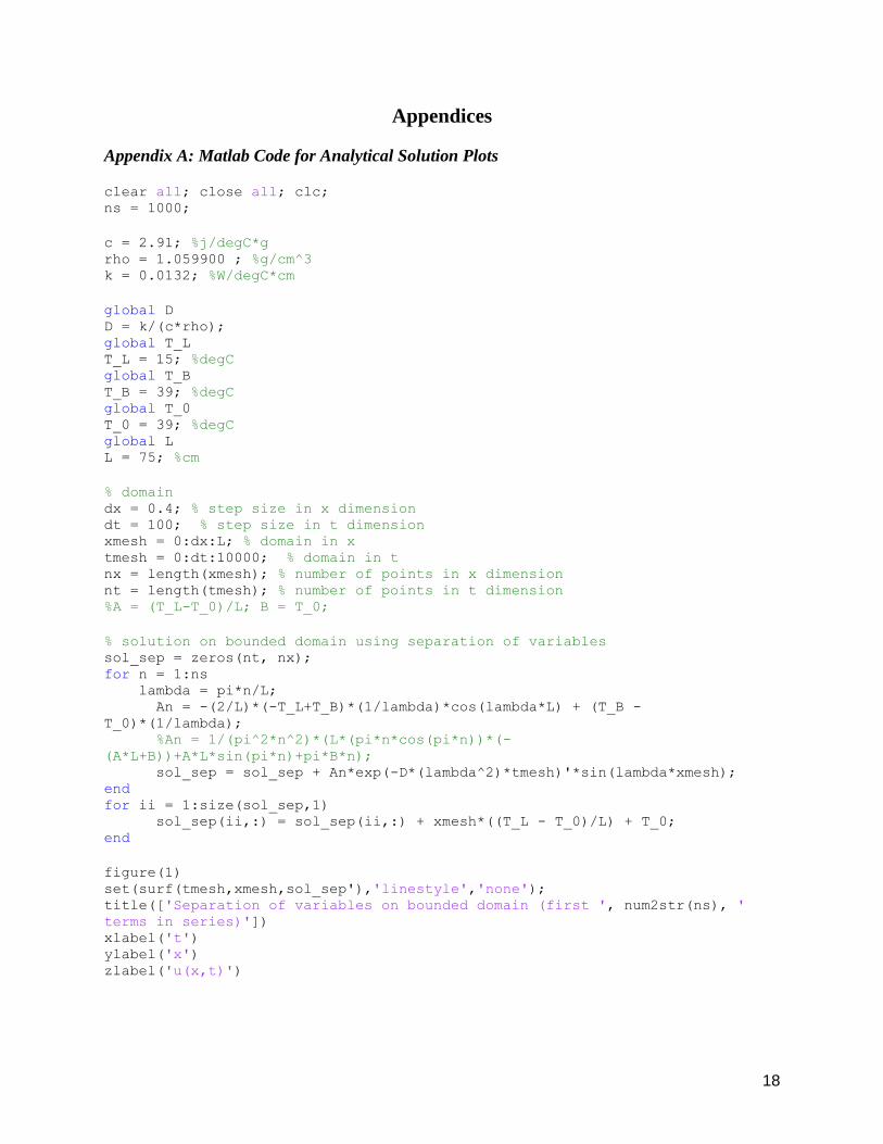
Appendix A: Matlab Code for Analytical Solution Plots

clear all; close all; clc; ns = 1000;

c = 2.91; %j/degC*g rho = 1.059900 ; %g/cm^3 k = 0.0132; %W/degC*cm

global D D = k/(c*rho); global T_L T_L = 15; %degC global T_B T_B = 39; %degC global T_0 T_0 = 39; %degC global L L = 75; %cm

% domain dx = 0.4; % step size in x dimension dt = 100; % step size in t dimension xmesh = 0:dx:L; % domain in x tmesh = 0:dt:10000; % domain in t nx = length(xmesh); % number of points in x dimension nt = length(tmesh); % number of points in t dimension %A = (T_L-T_0)/L; B = T_0;

% solution on bounded domain using separation of variables sol_sep = zeros(nt, nx); for n = 1:ns lambda = pi*n/L; An = -(2/L)*(-T_L+T_B)*(1/lambda)*cos(lambda*L) + (T_B -

T_0)*(1/lambda); %An = 1/(pi^2*n^2)*(L*(pi*n*cos(pi*n))*(-

(A*L+B))+A*L*sin(pi*n)+pi*B*n); sol_sep = sol_sep + An*exp(-D*(lambda^2)*tmesh)'*sin(lambda*xmesh); end for ii = 1:size(sol_sep,1) sol_sep(ii,:) = sol_sep(ii,:) + xmesh*((T_L - T_0)/L) + T_0; end

figure(1) set(surf(tmesh,xmesh,sol_sep'),'linestyle','none'); title(['Separation of variables on bounded domain (first ', num2str(ns), '

terms in series)']) xlabel('t') ylabel('x') zlabel('u(x,t)')

19

Appendix B: Matlab Code for Numerical Solution Plots with pdepe and Heat Dissipation

Calculation

function BENG221_proj

% diffusion constant

c = 2.91; %j/degC*g

rho = 1.0599 ; %g/cm^3

k = .0132; %W/degC*cm

global D T_B T_L

D = k/(c*rho);

T_L = 15; %degC

T_B = 37; %degC

T_0 = 39; %degC

L = 75; %cm

% domain

dx = 1; % step size in x dimension

dt = 100; % step size in t dimension

xmesh = 0:dx:L; % domain in x

tmesh = 0:dt:10000; % domain in t

% solution using finite differences

nx = length(xmesh); % number of points in x dimension

nt = length(tmesh); % number of points in t dimension

% solution using Matlab's built in "pdepe"

sol_pdepe = pdepe(0,@pdefun,@ic,@bc,xmesh,tmesh);

figure(2)

surf(tmesh,xmesh,sol_pdepe')

title('Normal body temp (37) and device temp (15)')

xlabel('t')

ylabel('x')

zlabel('u(x,t)')

totalValue = 0;

tempdif=1*L*c*rho*5.08^2*pi

for jj=1:nt

totalValue = 0;

for ii=1:nx-1

totalValue=totalValue+dx*(T_B-(sol_pdepe(jj,ii)+sol_pdepe(jj,ii+1))/2)*c*rho*5.08^2*pi;

end

if totalValue>tempdif

tempdif=10000000;

time2reach=jj

totalValue2=totalValue

end

end

%heatlost=(totalValue)*c*rho*5.08^2*pi

20

heatlost=totalValue

thelost=T_B*L*c*rho*5.08^2*pi

% function definitions for pdepe:

function [c, f, s] = pdefun(x, t, u, DuDx)

% PDE coefficients functions

global D

c = 1;

f = D * DuDx; % diffusion

s = 0; % homogeneous, no driving term

function u0 = ic(x)

% Initial conditions function

%C0=1;

global T_B

u0 = T_B; % heaviside plateau at center

function [pl, ql, pr, qr] = bc(xl, ul, xr, ur, t)

% Boundary conditions function

global T_B T_L

pl = ul-T_B;

ql = 0;

pr = ur-T_L;

qr = 0;

References

[1] D. Wendt, L. Van Loon and W. Lichtenbelt, 'Thermoregulation during exercise in the

heat',Sports Medicine, vol. 37, no. 8, pp. 669--682, 2007.

[2] Jones, S., Martin, R., & Pilbeam, D. (1994) The Cambridge Encyclopedia of Human

Evolution". Cambridge: Cambridge University Press

[3] http://www.avacore.com/enhancing-thermal-exchange-humans-and-practical-applications

[4] American Orthopaedic Society for Sports Medicine 34: 1953-1969 (2006)

[5] D. Grahn, V. Cao and H. Heller, 'Heat extraction through the palm of one hand improves

aerobic exercise endurance in a hot environment', Journal of Applied Physiology, vol. 99, no. 3,

pp. 972--978, 2005.

[6] D. Grahn, V. Cao, C. Nguyen, M. Liu and H. Heller, 'Work volume and strength training

responses to resistive exercise improve with periodic heat extraction from the palm', The Journal

of Strength \& Conditioning Research, vol. 26, no. 9, pp. 2558--2569, 2012.

[7] J. Gonzalez-Alonso, B. Quistorff, P. Krustrup, J. Bangsbo and B. Saltin, 'Heat production in

human skeletal muscle at the onset of intense dynamic exercise', The Journal of physiology, vol.

524, no. 2, pp. 603--615, 2000.

[8] M. DUCHARME and P. TIKUISIS, 'In vivo thermal conductivity of the human forearm

tissues',Journal of Applied Physiology, vol. 70, no. 6, pp. 2681--2690, 1991.

21

[9] M. Urbanchek, E. Picken, L. Kalliainen and W. Kuzon, 'Specific force deficit in skeletal

muscles of old rats is partially explained by the existence of denervated muscle fibers', The

Journals of Gerontology Series A: Biological Sciences and Medical Sciences, vol. 56, no. 5, pp.

191--197, 2001.

[10] http://www.ncbi.nlm.nih.gov/pubmed/15879169

[11] L. Jiji, Heat conduction. Berlin: Springer, 2009.

[12] R. Haberman, Elementary applied partial differential equations. Englewood Ciffs, N.J.:

Prentice-Hall, 1987.