math mode – v.2

Math mode – v. 2.47

Herbert Voß*

January 30, 2014

Abstract

It is often said that TEX was designed for mathematical or technical purposes.This may be true when we remember the reasons why Donald Knuth created TEX.But nowadays there are many examples in which TEX is used for publicationswith no mathematical or technical background content. However, writing publi-cations with such material is one of the important advantages of TEX. Becauseit seems impossible to know all existing macros and options of (LA)TEX and theseveral additional packages, especially of AMSmath. This is the reason whyI have attempted to gather all the relevant facts in this paper. An advancedversion of this paper is available as a german book [25] and also as an englishtranslation [27]. Members of DANTE e. V., the german TEX users group, may askfor a special price of the german edition (http://www.dante.de)!

Please report typos or any other comments to this documentation to [email protected] file can be redistributed and/or modified under the terms of the LATEX

Project Public License Distributed from CTAN archives in directory CTAN://macros/latex/base/lppl.txt.

*Thanks for the feedback to: Hendri Adriaens; Juan Mari Alberdi; Luciano Battaia; Heiko Bauke;Neal Becker; Andrea Blomenhofer; Alexander Boronka; Walter Brown; Alexander Buchner; WilhelmBurger; Marco Daniel; Christian Faulhammer; José Luis Gómez Dans; Zongbao Fang; Sabine Glaser;Sven Gleich; Azzam Hassam; Gernot Hassenpflug; Henning Heinze; Martin Hensel; Mathias Hoffmann;Jon Kirwan; Morten Høgholm; M. Kalidoss; Dan Lasley; Angus Leeming; Vladimir Lomov; Mico Loretan;Tim Love; Ladislav Lukas; Dan Luecking; Hendrik Maryns; Heinz Mezera; David Neuway; Luis TruccoPassadore; Joachim Punter; Carl Riehm; Will Robertson; Christoph Rumsmüller; José Carlos Santos;Arnaud Schmittbuhl; Rainer Schöpf; Jens Schwaiger; Uwe Siart; Martin Sievers; Heiko Stamer; G.Stengert; Uwe Stöhr; Guangjun Tan; Carsten Thiel; Juan Luis Varona; David Weenink; Philipp Wook;Michael Zedler; Zou Yuan-Chuan; and last but not least a special thanks to Monika Hattenbach for herexcellent job of proofreading.

1

http://www.dante.de

mailto:[email protected]

CTAN://macros/latex/base/lppl.txt

CTAN://macros/latex/base/lppl.txt

CONTENTS CONTENTS

Contents

Page

I Standard LATEX math mode 9

1 Introduction 9

2 The Inlinemode 9

2.1 Limits . . . . . . . . . . . . . . . . . . . . . . . . . . . . . . . . . . 9

2.2 Fraction command . . . . . . . . . . . . . . . . . . . . . . . . . . . 10

2.3 Math in Chapter/Section Titles . . . . . . . . . . . . . . . . . . . . 10

2.4 Equation numbering . . . . . . . . . . . . . . . . . . . . . . . . . . 10

2.5 Framed math . . . . . . . . . . . . . . . . . . . . . . . . . . . . . . 11

2.6 Linebreak . . . . . . . . . . . . . . . . . . . . . . . . . . . . . . . . 11

2.7 Whitespace . . . . . . . . . . . . . . . . . . . . . . . . . . . . . . . 11

2.8 AMSmath for the inline mode . . . . . . . . . . . . . . . . . . . . 11

3 Displaymath mode 12

3.1 equation environment . . . . . . . . . . . . . . . . . . . . . . . . . 12

3.2 eqnarray environment . . . . . . . . . . . . . . . . . . . . . . . . . 13

3.2.1 Short commands . . . . . . . . . . . . . . . . . . . . . . . . . 13

3.3 Equation numbering . . . . . . . . . . . . . . . . . . . . . . . . . . 14

3.3.1 Changing the style . . . . . . . . . . . . . . . . . . . . . . . 14

3.3.2 Resetting a counter style . . . . . . . . . . . . . . . . . . . . 14

3.3.3 Equation numbers on the left side . . . . . . . . . . . . . . . 15

3.3.4 Changing the equation number style . . . . . . . . . . . . . 15

3.3.5 More than one equation counter . . . . . . . . . . . . . . . . 15

3.4 Labels . . . . . . . . . . . . . . . . . . . . . . . . . . . . . . . . . . 16

3.5 Frames . . . . . . . . . . . . . . . . . . . . . . . . . . . . . . . . . 16

4 array environment 17

4.1 Cases structure . . . . . . . . . . . . . . . . . . . . . . . . . . . . . 18

4.2 arraycolsep . . . . . . . . . . . . . . . . . . . . . . . . . . . . . . 19

5 Matrix 20

6 Super/Subscript and limits 22

6.1 Multiple limits . . . . . . . . . . . . . . . . . . . . . . . . . . . . . 22

6.2 Problems . . . . . . . . . . . . . . . . . . . . . . . . . . . . . . . . 23

7 Roots 23

8 Brackets, braces . . . 24

8.1 Examples . . . . . . . . . . . . . . . . . . . . . . . . . . . . . . . . 27

8.1.1 Braces over several lines . . . . . . . . . . . . . . . . . . . . 27

8.1.2 Middle bar . . . . . . . . . . . . . . . . . . . . . . . . . . . . 28

8.2 New delimiters . . . . . . . . . . . . . . . . . . . . . . . . . . . . . 28

8.3 Problems with parentheses . . . . . . . . . . . . . . . . . . . . . . 28

9 Text in math mode 29

2 MathmodeOrig.tex v.2.47

CONTENTS CONTENTS

10Font commands 2910.1 Old-style font commands . . . . . . . . . . . . . . . . . . . . . . . 29

10.2 New-style font commands . . . . . . . . . . . . . . . . . . . . . . . 30

11Space 3011.1 Math typesetting . . . . . . . . . . . . . . . . . . . . . . . . . . . . 30

11.2 Additional horizontal spacing . . . . . . . . . . . . . . . . . . . . . 31

11.3 Problems . . . . . . . . . . . . . . . . . . . . . . . . . . . . . . . . 32

11.4 Dot versus comma . . . . . . . . . . . . . . . . . . . . . . . . . . . 32

11.5 Vertical whitespace . . . . . . . . . . . . . . . . . . . . . . . . . . 33

11.5.1 Before/after math expressions . . . . . . . . . . . . . . . . . 33

11.5.2 Inside math expressions . . . . . . . . . . . . . . . . . . . . 34

12Styles 36

13Dots 37

14Accents 3714.1 Over- and underbrackets . . . . . . . . . . . . . . . . . . . . . . . 37

14.1.1 Use of \underbracket... . . . . . . . . . . . . . . . . . . 38

14.1.2 Overbracket . . . . . . . . . . . . . . . . . . . . . . . . . . . 38

14.2 Vectors . . . . . . . . . . . . . . . . . . . . . . . . . . . . . . . . . 39

15Exponents and indices 39

16Operators 40

17Greek letters 41

18Pagebreaks 42

19\stackrel 42

20\choose 43

21Color in math expressions 43

22Boldmath 4322.1 Bold math titles and items . . . . . . . . . . . . . . . . . . . . . . 44

23Multiplying numbers 45

24Other macros 45

II AMSmath package 46

25align environments 4625.1 The default align environment . . . . . . . . . . . . . . . . . . . . 47

25.2 alignat environment . . . . . . . . . . . . . . . . . . . . . . . . . 48

25.3 flalign environment . . . . . . . . . . . . . . . . . . . . . . . . . 49

25.4 xalignat environment . . . . . . . . . . . . . . . . . . . . . . . . . 51

25.5 xxalignat environment . . . . . . . . . . . . . . . . . . . . . . . . 51

25.6 aligned environment . . . . . . . . . . . . . . . . . . . . . . . . . 51

MathmodeOrig.tex v.2.47 3

CONTENTS CONTENTS

25.7 Problems . . . . . . . . . . . . . . . . . . . . . . . . . . . . . . . . 52

26Other environments 52

26.1 gather environment . . . . . . . . . . . . . . . . . . . . . . . . . . 52

26.2 gathered environment . . . . . . . . . . . . . . . . . . . . . . . . . 53

26.3 multline environment . . . . . . . . . . . . . . . . . . . . . . . . . 54

26.3.1 Examples for multline . . . . . . . . . . . . . . . . . . . . . 55

26.4 split environment . . . . . . . . . . . . . . . . . . . . . . . . . . . 57

26.5 cases environment . . . . . . . . . . . . . . . . . . . . . . . . . . 59

26.6 Matrix environments . . . . . . . . . . . . . . . . . . . . . . . . . . 60

27Vertical whitespace 60

28Dots 60

29fraction commands 61

29.1 Standard . . . . . . . . . . . . . . . . . . . . . . . . . . . . . . . . 61

29.2 Binoms . . . . . . . . . . . . . . . . . . . . . . . . . . . . . . . . . 62

30Roots 62

30.1 Roots with \smash command . . . . . . . . . . . . . . . . . . . . . 63

31Accents 63

32\mod command 63

33Equation numbering 64

33.1 Subequations . . . . . . . . . . . . . . . . . . . . . . . . . . . . . . 64

34Labels and tags 65

35Limits 66

35.1 Multiple limits . . . . . . . . . . . . . . . . . . . . . . . . . . . . . 66

35.2 Problems . . . . . . . . . . . . . . . . . . . . . . . . . . . . . . . . 66

35.3 \sideset . . . . . . . . . . . . . . . . . . . . . . . . . . . . . . . . 68

36Operator names 68

37Text in math mode 69

37.1 \text command . . . . . . . . . . . . . . . . . . . . . . . . . . . . 69

37.2 \intertext command . . . . . . . . . . . . . . . . . . . . . . . . . 70

38Extensible arrows 70

39Frames 72

40Greek letters 72

41Miscellaneous commands 73

42Problems with amsmath 73

III TEX and math 75


CONTENTS CONTENTS

43Length registers 75

43.1 \abovedisplayshortskip . . . . . . . . . . . . . . . . . . . . . . . 75

43.2 \abovedisplayskip . . . . . . . . . . . . . . . . . . . . . . . . . . 75

43.3 \belowdisplayshortskip . . . . . . . . . . . . . . . . . . . . . . . 75

43.4 \belowdisplayskip . . . . . . . . . . . . . . . . . . . . . . . . . . 75

43.5 \delimiterfactor . . . . . . . . . . . . . . . . . . . . . . . . . . . 75

43.6 \delimitershortfall . . . . . . . . . . . . . . . . . . . . . . . . . 76

43.7 \displayindent . . . . . . . . . . . . . . . . . . . . . . . . . . . . 76

43.8 \displaywidth . . . . . . . . . . . . . . . . . . . . . . . . . . . . . 77

43.9 \mathsurround . . . . . . . . . . . . . . . . . . . . . . . . . . . . . 77

43.10 \medmuskip . . . . . . . . . . . . . . . . . . . . . . . . . . . . . . . 77

43.11 \mkern . . . . . . . . . . . . . . . . . . . . . . . . . . . . . . . . . . 77

43.12 \mskip . . . . . . . . . . . . . . . . . . . . . . . . . . . . . . . . . . 77

43.13 \muskip . . . . . . . . . . . . . . . . . . . . . . . . . . . . . . . . . 78

43.14 \muskipdef . . . . . . . . . . . . . . . . . . . . . . . . . . . . . . . 78

43.15 \nonscript . . . . . . . . . . . . . . . . . . . . . . . . . . . . . . . 78

43.16 \nulldelimiterspace . . . . . . . . . . . . . . . . . . . . . . . . . 78

43.17 \predisplaysize . . . . . . . . . . . . . . . . . . . . . . . . . . . 78

43.18 \scriptspace . . . . . . . . . . . . . . . . . . . . . . . . . . . . . . 78

43.19 \thickmuskip . . . . . . . . . . . . . . . . . . . . . . . . . . . . . . 78

43.20 \thinmuskip . . . . . . . . . . . . . . . . . . . . . . . . . . . . . . 78

43.21 \medmuskip . . . . . . . . . . . . . . . . . . . . . . . . . . . . . . . 79

44Math font macros 79

44.1 \delcode . . . . . . . . . . . . . . . . . . . . . . . . . . . . . . . . 79

44.2 \delimiter . . . . . . . . . . . . . . . . . . . . . . . . . . . . . . . 79

44.3 \displaystyle . . . . . . . . . . . . . . . . . . . . . . . . . . . . . 80

44.4 \fam . . . . . . . . . . . . . . . . . . . . . . . . . . . . . . . . . . . 80

44.5 \mathaccent . . . . . . . . . . . . . . . . . . . . . . . . . . . . . . 80

44.6 \mathbin . . . . . . . . . . . . . . . . . . . . . . . . . . . . . . . . 81

44.7 \mathchar . . . . . . . . . . . . . . . . . . . . . . . . . . . . . . . . 81

44.8 \mathchardef . . . . . . . . . . . . . . . . . . . . . . . . . . . . . . 81

44.9 \mathchoice . . . . . . . . . . . . . . . . . . . . . . . . . . . . . . 81

44.10 \mathclose . . . . . . . . . . . . . . . . . . . . . . . . . . . . . . . 82

44.11 \mathcode . . . . . . . . . . . . . . . . . . . . . . . . . . . . . . . . 82

44.12 \mathop . . . . . . . . . . . . . . . . . . . . . . . . . . . . . . . . . 82

44.13 \mathopen . . . . . . . . . . . . . . . . . . . . . . . . . . . . . . . . 82

44.14 \mathord . . . . . . . . . . . . . . . . . . . . . . . . . . . . . . . . 82

44.15 \mathpunct . . . . . . . . . . . . . . . . . . . . . . . . . . . . . . . 83

44.16 \mathrel . . . . . . . . . . . . . . . . . . . . . . . . . . . . . . . . 83

44.17 \scriptfont . . . . . . . . . . . . . . . . . . . . . . . . . . . . . . 83

44.18 \scriptscriptfont . . . . . . . . . . . . . . . . . . . . . . . . . . 83

44.19 \scriptscriptstyle . . . . . . . . . . . . . . . . . . . . . . . . . 83

44.20 \scriptstyle . . . . . . . . . . . . . . . . . . . . . . . . . . . . . . 83

44.21 \skew . . . . . . . . . . . . . . . . . . . . . . . . . . . . . . . . . . 83

44.22 \skewchar . . . . . . . . . . . . . . . . . . . . . . . . . . . . . . . . 84

44.23 \textfont . . . . . . . . . . . . . . . . . . . . . . . . . . . . . . . . 84

44.24 \textstyle . . . . . . . . . . . . . . . . . . . . . . . . . . . . . . . 84


CONTENTS CONTENTS

45Math macros 8445.1 \above . . . . . . . . . . . . . . . . . . . . . . . . . . . . . . . . . . 84

45.2 \abovewithdelims . . . . . . . . . . . . . . . . . . . . . . . . . . . 84

45.3 \atop . . . . . . . . . . . . . . . . . . . . . . . . . . . . . . . . . . 85

45.4 \atopwithdelims . . . . . . . . . . . . . . . . . . . . . . . . . . . 85

45.5 \displaylimits . . . . . . . . . . . . . . . . . . . . . . . . . . . . 85

45.6 \eqno . . . . . . . . . . . . . . . . . . . . . . . . . . . . . . . . . . 85

45.7 \everydisplay . . . . . . . . . . . . . . . . . . . . . . . . . . . . . 86

45.8 \everymath . . . . . . . . . . . . . . . . . . . . . . . . . . . . . . . 86

45.9 \left . . . . . . . . . . . . . . . . . . . . . . . . . . . . . . . . . . 86

45.10 \leqno . . . . . . . . . . . . . . . . . . . . . . . . . . . . . . . . . . 86

45.11 \limits . . . . . . . . . . . . . . . . . . . . . . . . . . . . . . . . . 87

45.12 \mathinner . . . . . . . . . . . . . . . . . . . . . . . . . . . . . . . 87

45.13 \nolimits . . . . . . . . . . . . . . . . . . . . . . . . . . . . . . . . 87

45.14 \over . . . . . . . . . . . . . . . . . . . . . . . . . . . . . . . . . . 87

45.15 \overline . . . . . . . . . . . . . . . . . . . . . . . . . . . . . . . . 87

45.16 \overwithdelims . . . . . . . . . . . . . . . . . . . . . . . . . . . 87

45.17 \radical . . . . . . . . . . . . . . . . . . . . . . . . . . . . . . . . 88

45.18 \right . . . . . . . . . . . . . . . . . . . . . . . . . . . . . . . . . . 88

45.19 \underline . . . . . . . . . . . . . . . . . . . . . . . . . . . . . . . 88

45.20 \vcenter . . . . . . . . . . . . . . . . . . . . . . . . . . . . . . . . 88

46Math penalties 8846.1 \binoppenalty . . . . . . . . . . . . . . . . . . . . . . . . . . . . . 88

46.2 \displaywidowpenalty . . . . . . . . . . . . . . . . . . . . . . . . 89

46.3 \postdisplaypenalty . . . . . . . . . . . . . . . . . . . . . . . . . 89

46.4 \predisplaypenalty . . . . . . . . . . . . . . . . . . . . . . . . . 89

46.5 \relpenalty . . . . . . . . . . . . . . . . . . . . . . . . . . . . . . 89

IV Other packages 90

47List of available math packages 9047.1 accents . . . . . . . . . . . . . . . . . . . . . . . . . . . . . . . . . 90

47.2 amscd – commutative diagrams . . . . . . . . . . . . . . . . . . . . 90

47.3 amsopn . . . . . . . . . . . . . . . . . . . . . . . . . . . . . . . . . . 91

47.4 bigdel . . . . . . . . . . . . . . . . . . . . . . . . . . . . . . . . . . 91

47.5 bm . . . . . . . . . . . . . . . . . . . . . . . . . . . . . . . . . . . . 92

47.6 braket . . . . . . . . . . . . . . . . . . . . . . . . . . . . . . . . . . 92

47.7 cancel . . . . . . . . . . . . . . . . . . . . . . . . . . . . . . . . . . 94

47.8 cool . . . . . . . . . . . . . . . . . . . . . . . . . . . . . . . . . . . 94

47.9 delarray . . . . . . . . . . . . . . . . . . . . . . . . . . . . . . . . 95

47.10 dotseqn . . . . . . . . . . . . . . . . . . . . . . . . . . . . . . . . . 96

47.11 empheq . . . . . . . . . . . . . . . . . . . . . . . . . . . . . . . . . . 96

47.12 esint . . . . . . . . . . . . . . . . . . . . . . . . . . . . . . . . . . 97

47.13 eucal and euscript . . . . . . . . . . . . . . . . . . . . . . . . . . 98

47.14 exscale . . . . . . . . . . . . . . . . . . . . . . . . . . . . . . . . . 98

47.15 mathtools . . . . . . . . . . . . . . . . . . . . . . . . . . . . . . . . 99

47.16 nicefrac . . . . . . . . . . . . . . . . . . . . . . . . . . . . . . . . 100

47.17 relsize . . . . . . . . . . . . . . . . . . . . . . . . . . . . . . . . . 100


CONTENTS CONTENTS

47.18 xypic . . . . . . . . . . . . . . . . . . . . . . . . . . . . . . . . . . 101

V Math fonts 102

48Computer modern 102

49Latin modern 102

50Palatino 103

51Palatino – microimp 103

52cmbright 104

53minion 104

VI Special symbols 105

54Integral symbols 105

55Harpoons 106

56Bijective mapping arrow 106

57Stacked equal sign 107

58Other symbols 107

VII Examples 108

59Tuning math typesetting 108

60Matrix 109

60.1 Identity matrix . . . . . . . . . . . . . . . . . . . . . . . . . . . . . 109

60.2 System of linear equations . . . . . . . . . . . . . . . . . . . . . . 109

60.3 Matrix with comments on top . . . . . . . . . . . . . . . . . . . . . 110

61Cases structure 110

61.1 Cases with numbered lines . . . . . . . . . . . . . . . . . . . . . . 111

62Arrays 112

62.1 Quadratic equation . . . . . . . . . . . . . . . . . . . . . . . . . . . 112

62.2 Vectors and matrices . . . . . . . . . . . . . . . . . . . . . . . . . . 113

62.3 Cases with (eqn)array environment . . . . . . . . . . . . . . . . . 113

62.4 Arrays inside arrays . . . . . . . . . . . . . . . . . . . . . . . . . . 114

62.5 Colored cells . . . . . . . . . . . . . . . . . . . . . . . . . . . . . . 115

62.6 Boxed rows and columns . . . . . . . . . . . . . . . . . . . . . . . 115

63Over- and underbraces 116

63.1 Braces and roots . . . . . . . . . . . . . . . . . . . . . . . . . . . . 116

63.2 Overlapping braces . . . . . . . . . . . . . . . . . . . . . . . . . . 117

63.3 Vertical alignment . . . . . . . . . . . . . . . . . . . . . . . . . . . 117


CONTENTS CONTENTS

63.4 Alignment . . . . . . . . . . . . . . . . . . . . . . . . . . . . . . . . 118

64Integrals 119

65Horizontal alignment 12065.1 Over more than one page . . . . . . . . . . . . . . . . . . . . . . . 12065.2 Special text columns . . . . . . . . . . . . . . . . . . . . . . . . . . 12165.3 Centered vertical dots . . . . . . . . . . . . . . . . . . . . . . . . . 123

66Node connections 123

67Special Placement 12467.1 Formulas side by side . . . . . . . . . . . . . . . . . . . . . . . . . 12467.2 Itemize environment . . . . . . . . . . . . . . . . . . . . . . . . . . 126

68Roots 127

VIII Lists, bibliography and index 128

List of Figures 129

List of Tables 130

Bibliography 131

Index 133

A Filelist 141


2 THE INLINEMODE

Part I

Standard LATEX math mode

1 Introduction

The following sections describe all the math commands which are available withoutany additional package. Most of them also work with special packages and some ofthem are redefined. At first some important facts for typesetting math expressions.

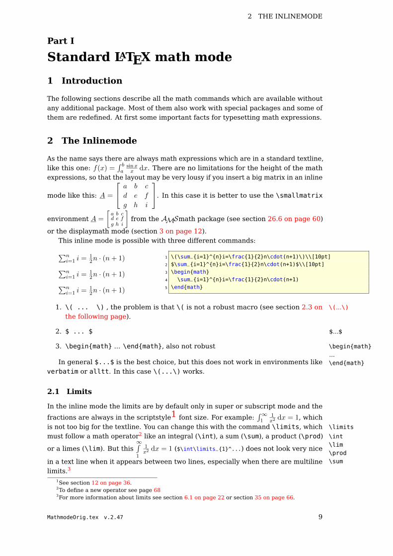
2 The Inlinemode

As the name says there are always math expressions which are in a standard textline,like this one: f(x) =

´ ba

sinxx dx. There are no limitations for the height of the math

expressions, so that the layout may be very lousy if you insert a big matrix in an inline

mode like this: A =

a b c

d e f

g h i

. In this case it is better to use the \smallmatrix

environment A =

[a b cd e fg h i

]from the AMSmath package (see section 26.6 on page 60)

or the displaymath mode (section 3 on page 12).This inline mode is possible with three different commands:

∑ni=1 i = 1

2n · (n+ 1)

∑ni=1 i = 1

2n · (n+ 1)

∑ni=1 i = 1

2n · (n+ 1)

1 $\sum_i=1^ni=\frac12n\cdot(n+1)$\\[10pt]2 $\sum_i=1^ni=\frac12n\cdot(n+1)$\\[10pt]3 \beginmath4 \sum_i=1^ni=\frac12n\cdot(n+1)5 \endmath

1. $ ... $ , the problem is that $ is not a robust macro (see section 2.3 on \(...$

the following page).

2. $ ... $ $...$

3. \beginmath ... \endmath, also not robust \beginmath...\endmathIn general $...$ is the best choice, but this does not work in environments like

verbatim or alltt. In this case $...$ works.

2.1 Limits

In the inline mode the limits are by default only in super or subscript mode and the

fractions are always in the scriptstyle1 font size. For example:´∞

11x2

dx = 1, whichis not too big for the textline. You can change this with the command \limits, which \limits

must follow a math operator2 like an integral (\int), a sum (\sum), a product (\prod) \int\lim\prod\sum

or a limes (\lim). But this∞

1

1x2

dx = 1 ($\int\limits_1^...) does not look very nice

in a text line when it appears between two lines, especially when there are multilinelimits.3

1See section 12 on page 36.2To define a new operator see page 683For more information about limits see section 6.1 on page 22 or section 35 on page 66.


2 THE INLINEMODE 2.2 Fraction command

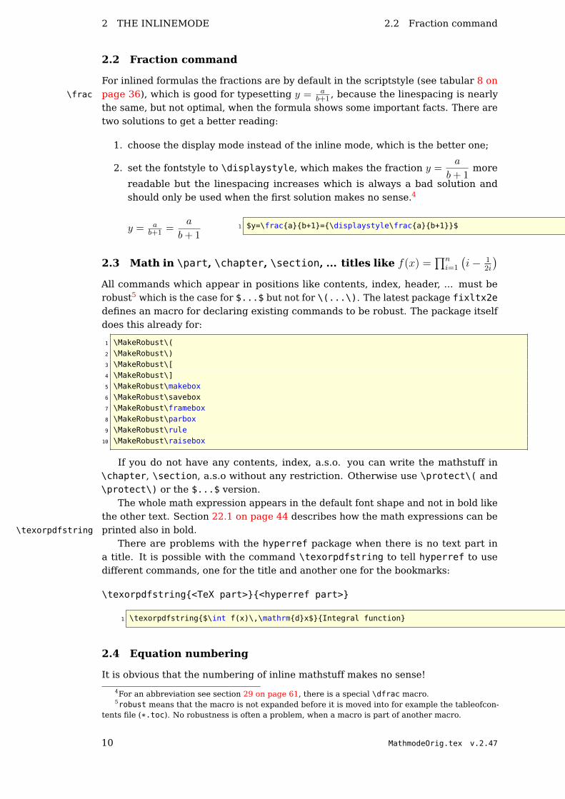
2.2 Fraction command

For inlined formulas the fractions are by default in the scriptstyle (see tabular 8 onpage 36), which is good for typesetting y = a

b+1 , because the linespacing is nearly\frac

the same, but not optimal, when the formula shows some important facts. There aretwo solutions to get a better reading:

1. choose the display mode instead of the inline mode, which is the better one;

2. set the fontstyle to \displaystyle, which makes the fraction y =a

b+ 1more

readable but the linespacing increases which is always a bad solution andshould only be used when the first solution makes no sense.4

y = ab+1 =

a

b+ 11 $y=\fracab+1=\displaystyle\fracab+1$

2.3 Math in \part, \chapter, \section, ... titles like f(x) =∏n

i=1

(i− 1

2i

)

All commands which appear in positions like contents, index, header, ... must berobust5 which is the case for $...$ but not for $...$. The latest package fixltx2edefines an macro for declaring existing commands to be robust. The package itselfdoes this already for:

1 \MakeRobust$2 \MakeRobust$3 \MakeRobust\[4 \MakeRobust\]5 \MakeRobust\makebox6 \MakeRobust\savebox7 \MakeRobust\framebox8 \MakeRobust\parbox9 \MakeRobust\rule

10 \MakeRobust\raisebox

If you do not have any contents, index, a.s.o. you can write the mathstuff in\chapter, \section, a.s.o without any restriction. Otherwise use \protect$ and\protect$ or the $...$ version.

The whole math expression appears in the default font shape and not in bold likethe other text. Section 22.1 on page 44 describes how the math expressions can beprinted also in bold.\texorpdfstring

There are problems with the hyperref package when there is no text part ina title. It is possible with the command \texorpdfstring to tell hyperref to usedifferent commands, one for the title and another one for the bookmarks:

\texorpdfstring<TeX part><hyperref part>

1 \texorpdfstring$\int f(x)\,\mathrmdx$Integral function

2.4 Equation numbering

It is obvious that the numbering of inline mathstuff makes no sense!

4For an abbreviation see section 29 on page 61, there is a special \dfrac macro.5robust means that the macro is not expanded before it is moved into for example the tableofcon-

tents file (*.toc). No robustness is often a problem, when a macro is part of another macro.


2.5 Framed math 2 THE INLINEMODE

2.5 Framed math

With the \fbox macro everything of inline math can be framed, like the followingone:

f(x) =∏ni=1

(i− 1

2i

)1 \fbox$f(x)=\prod_i=1^n\left(i-\frac12i\right)$

Parameters are the width of \fboxsep and \fboxrule, the predefined values fromthe file latex.ltx are:

1 \fboxsep = 3pt2 \fboxrule = .4pt

The same is possible with the \colorbox f(x) =∏ni=1

(i− 1

2i

)from the color

package.

1 \colorboxyellow$f(x)=\prod_i=1^n\left(i-\frac12i\right)$

2.6 Linebreak

LATEX can break an inline formula only when a relation symbol (=, <,>, . . .) or abinary operation symbol (+,−, . . .) exists and at least one of these symbols appears atthe outer level of a formula. Thus $a+b+c$ can be broken across lines, but $a+b+c$not.

• The default: f(x) = anxn+an−1x

n−1+an−2xn−2+. . .+aix

i+a2x2+a1x

1+a0

• The same inside a group ...: f(x) = anxn + an−1x

n−1 + an−2xn−2 + . . .+ aix

i + a2x2 + a1x

1 + a0

• Without any symbol: f(x) = an (an−1 (an−2 (. . .) . . .) . . .)

If it is not possible to have any mathsymbol, then split the inline formula in two ormore pieces ($...$ $...$). If you do not want a linebreak for the whole document,you can set in the preamble:

\relpenalty=9999\binoppenalty=9999

which is the extreme case of grudgingly allowing breaks in extreme cases, or

\relpenalty=10000\binoppenalty=10000

for absolutely no breaks.

2.7 Whitespace

LATEX defines the length \mathsurround with the default value of 0pt. This length isadded before and after an inlined math expression (see table 1 on the next page).

2.8 AMSmath for the inline mode

None of the AMSmath-functions are available in inline mode.


3 DISPLAYMATH MODE

foo f(x) =´∞

11x2

dx = 1 bar1 foo \fbox$ f(x)=\int_1^\infty\frac1x^2\,\mathrmdx=1 $

bar

foo f(x) =´∞

11x2

dx = 1 bar1 foo \rule20pt\ht\strutbox\fbox$ f(x)=\int_1^\infty\frac

1x^2\,\mathrmdx=1 $\rule20pt\ht\strutbox bar

foo f(x) =´∞

11x2

dx = 1 bar

1 \setlength\mathsurround20pt2 foo \fbox$ f(x)=\int_1^\infty\frac1x^2\,\mathrmdx=1 $

bar

Table 1: Meaning of \mathsurround

3 Displaymath mode

This means, that every formula gets its own paragraph (line). There are somedifferences in the layout to the one from the title of 2.3.

3.1 equation environment

For example:

f(x) =n∏

i=1

(i− 1

2i

)(1)

1 \beginequation2 f(x)=\prod_i=1^n\left(i-\frac12i\right)3 \endequation

The delimiters \beginequation ... \endequation are the only differenceto the inline version. There are some equivalent commands for the display-mathmode:\begindisplaymath

. . .\enddisplaymath

1. \begindisplaymath. . . \enddisplaymath, same as \[ . . . \]2. \[...\]. (see above) the short form of a displayed formula, no number

\[...\]

f(x) =

n∏

i=1

(i− 1

2i

)

displayed, no number. Same as 1.3. \beginequation...\endequation\beginequation

. . .\endequation

f(x) =n∏

i=1

(i− 1

2i

)(2)

displayed, a sequential equation number, which may be reset when starting anew chapter or section.(a) There is only one equation number for the whole environment.\nonumber(b) In standard LATEX there exists no star-version of the equation environment

because \[. . . \] is the equivalent. However, with package AMSmath itwill be defined. With the tag \nonumber it is possible to suppress theequation number:

f(x) = [...]

1 \beginequation2 f(x)= [...] \nonumber3 \endequation


3.2 eqnarray environment 3 DISPLAYMATH MODE

3.2 eqnarray environment

This is by default an array with three columns and as many rows as you like. It is \begineqnarray...\endeqnarray

nearly the same as an array with a rcl column definition.

It is not possible to change the internal behaviour of the eqnarray environmentwithout rewriting the environment. It is always an implicit array with three columnsand the horizontal alignment right-center-left (rcl) and small symbol sizes forthe middle column. All this can not be changed by the user without rewriting thewhole environment in latex.ltx.

left middle right1√n

=√nn =

n

n√n

1 \begineqnarray*2 \mathrmleft & \mathrmmiddle & \mathrmright\\3 \frac1\sqrtn= & \frac\sqrtnn= & \fracnn\

sqrtn4 \endeqnarray*

The eqnarray environment should not be used as an array. As seen in the aboveexample the typesetting is wrong for the middle column. The numbering of eqnarrayenvironments is always for every row, means, that four lines get four differentequation numbers (for the labels see section 3.4 on page 16):

y = d (3)

y = cx+ d (4)

y = bx2 + cx+ d (5)

y = ax3 + bx2 + cx+ d (6)

1 \begineqnarray2 y & = & d\labeleq:2\\3 y & = & cx+d\\4 y & = & bx^2+cx+d\\5 y & = & ax^3+bx^2+cx+d\labeleq:56 \endeqnarray

Suppressing the numbering for all rows is possible with the starred version ofeqnarray.

y = d

y = cx+ d

y = bx2 + cx+ d

y = ax3 + bx2 + cx+ d

1 \begineqnarray*2 y & = & d\labeleq:3\\3 y & = & cx+d\\4 y & = & bx^2+cx+d\\5 y & = & ax^3+bx^2+cx+d\labeleq:46 \endeqnarray*

Toggling off/on for single rows is possible with the above mentioned \nonumbertag at the end of a row (before the newline command). For example:

y = d

y = cx+ d

y = bx2 + cx+ d

y = ax3 + bx2 + cx+ d (7)

1 \begineqnarray2 y & = & d\nonumber \\3 y & = & cx+d\nonumber \\4 y & = & bx^2+cx+d\nonumber \\5 y & = & ax^3+bx^2+cx+d6 \endeqnarray

3.2.1 Short commands

It is possible to define short commands for the eqnarray environment

1 \makeatletter2 \newcommand\be%3 \begingroup4 % \setlength\arraycolsep2pt


3 DISPLAYMATH MODE 3.3 Equation numbering

5 \eqnarray%6 \@ifstar\nonumber%7 8 \newcommand\ee\endeqnarray\endgroup9 \makeatother

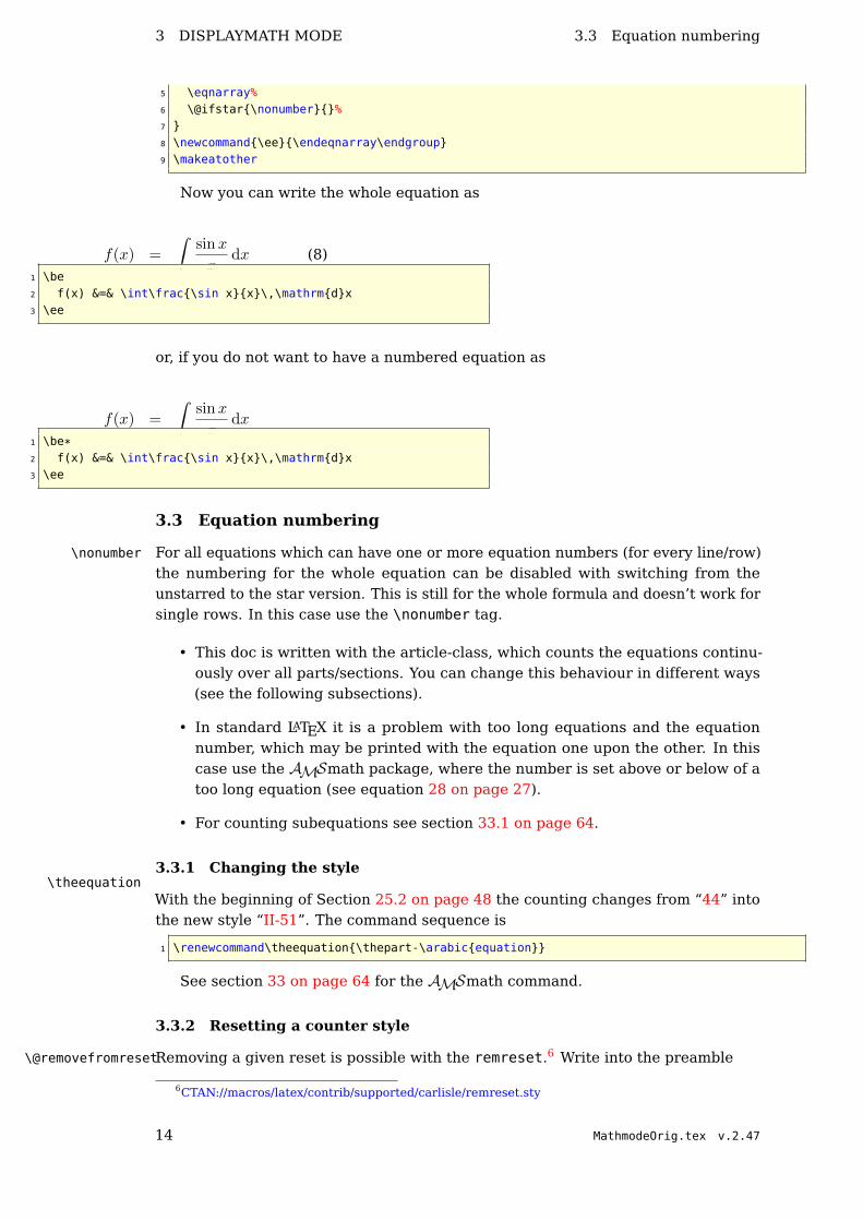
Now you can write the whole equation as

f(x) =

ˆsinx

xdx (8)

1 \be2 f(x) &=& \int\frac\sin xx\,\mathrmdx3 \ee

or, if you do not want to have a numbered equation as

f(x) =

ˆsinx

xdx

1 \be*2 f(x) &=& \int\frac\sin xx\,\mathrmdx3 \ee

3.3 Equation numbering

For all equations which can have one or more equation numbers (for every line/row)\nonumber

the numbering for the whole equation can be disabled with switching from theunstarred to the star version. This is still for the whole formula and doesn’t work forsingle rows. In this case use the \nonumber tag.

• This doc is written with the article-class, which counts the equations continu-ously over all parts/sections. You can change this behaviour in different ways(see the following subsections).

• In standard LATEX it is a problem with too long equations and the equationnumber, which may be printed with the equation one upon the other. In thiscase use the AMSmath package, where the number is set above or below of atoo long equation (see equation 28 on page 27).

• For counting subequations see section 33.1 on page 64.

3.3.1 Changing the style\theequation

With the beginning of Section 25.2 on page 48 the counting changes from “44” intothe new style “II-51”. The command sequence is

1 \renewcommand\theequation\thepart-\arabicequation

See section 33 on page 64 for the AMSmath command.

3.3.2 Resetting a counter style

Removing a given reset is possible with the remreset.6 Write into the preamble\@removefromreset

6CTAN://macros/latex/contrib/supported/carlisle/remreset.sty


http://www.ctan.org/tex-archive/macros/latex/contrib/supported/carlisle/remreset.sty

3.3 Equation numbering 3 DISPLAYMATH MODE

1 \makeatletter2 \@removefromresetequationsection3 \makeatother

or anywhere in the text.Now the equation counter is no longer reset when a new section starts. You can

see this after section 26.4 on page 57.

3.3.3 Equation numbers on the left side

Choose package leqno7 or have a look at your document class, if such an optionexists.

3.3.4 Changing the equation number style

The number style can be changed with a redefinition of

\def\@eqnnum\normalfont \normalcolor (\theequation)

For example: if you want the numbers not in parentheses write

1 \makeatletter2 \def\@eqnnum\normalfont \normalcolor \theequation3 \makeatother

For AMSmath there is another macro, see section 33 on page 64.

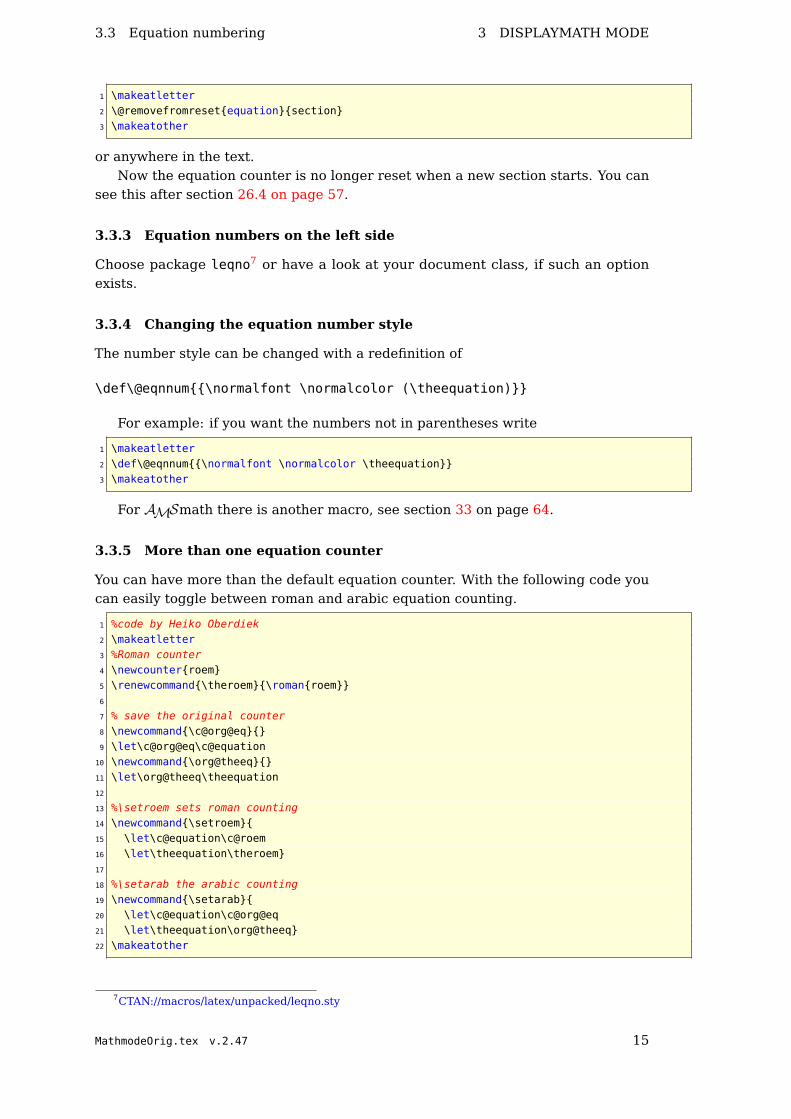
3.3.5 More than one equation counter

You can have more than the default equation counter. With the following code youcan easily toggle between roman and arabic equation counting.

1 %code by Heiko Oberdiek2 \makeatletter3 %Roman counter4 \newcounterroem5 \renewcommand\theroem\romanroem6

7 % save the original counter8 \newcommand\c@org@eq9 \let\c@org@eq\c@equation

10 \newcommand\org@theeq11 \let\org@theeq\theequation12

13 %\setroem sets roman counting14 \newcommand\setroem15 \let\c@equation\c@roem16 \let\theequation\theroem17

18 %\setarab the arabic counting19 \newcommand\setarab20 \let\c@equation\c@org@eq21 \let\theequation\org@theeq22 \makeatother

7CTAN://macros/latex/unpacked/leqno.sty


http://www.ctan.org/tex-archive/macros/latex/unpacked/leqno.sty

3 DISPLAYMATH MODE 3.4 Labels

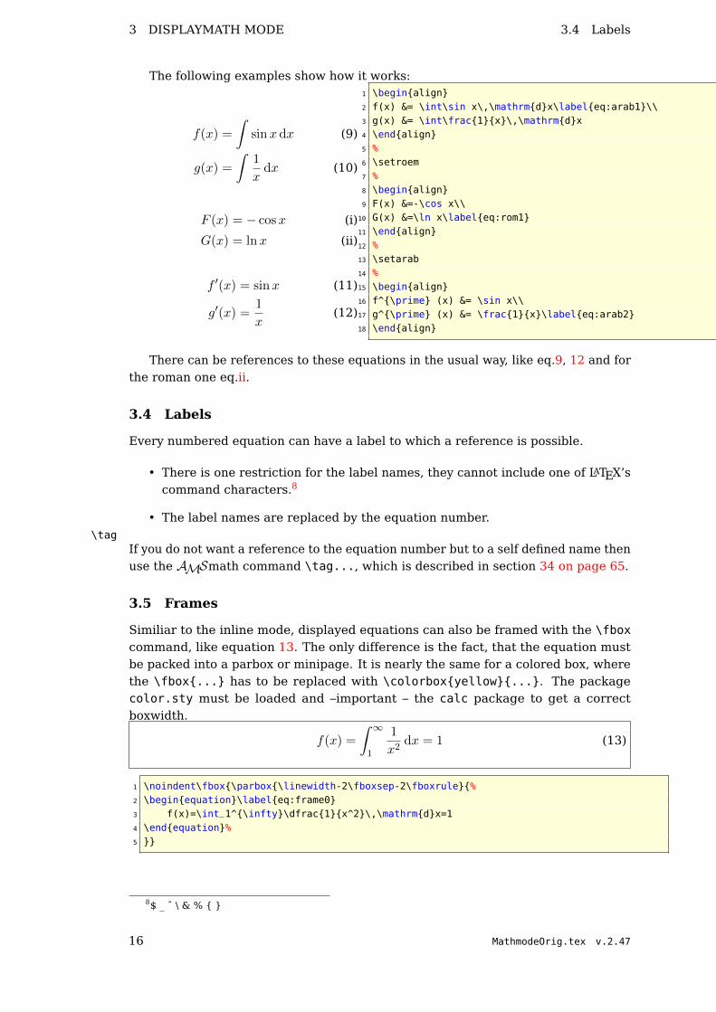
The following examples show how it works:

f(x) =

ˆsinx dx (9)

g(x) =

ˆ1

xdx (10)

F (x) = − cosx (i)

G(x) = lnx (ii)

f ′(x) = sinx (11)

g′(x) =1

x(12)

1 \beginalign2 f(x) &= \int\sin x\,\mathrmdx\labeleq:arab1\\3 g(x) &= \int\frac1x\,\mathrmdx4 \endalign5 %6 \setroem7 %8 \beginalign9 F(x) &=-\cos x\\

10 G(x) &=\ln x\labeleq:rom111 \endalign12 %13 \setarab14 %15 \beginalign16 f^\prime (x) &= \sin x\\17 g^\prime (x) &= \frac1x\labeleq:arab218 \endalign

There can be references to these equations in the usual way, like eq.9, 12 and forthe roman one eq.ii.

3.4 Labels

Every numbered equation can have a label to which a reference is possible.

• There is one restriction for the label names, they cannot include one of LATEX’scommand characters.8

• The label names are replaced by the equation number.\tag

If you do not want a reference to the equation number but to a self defined name thenuse the AMSmath command \tag..., which is described in section 34 on page 65.

3.5 Frames

Similiar to the inline mode, displayed equations can also be framed with the \fboxcommand, like equation 13. The only difference is the fact, that the equation mustbe packed into a parbox or minipage. It is nearly the same for a colored box, wherethe \fbox... has to be replaced with \colorboxyellow.... The packagecolor.sty must be loaded and –important – the calc package to get a correctboxwidth.

f(x) =

ˆ ∞1

1

x2dx = 1 (13)

1 \noindent\fbox\parbox\linewidth-2\fboxsep-2\fboxrule%2 \beginequation\labeleq:frame03 f(x)=\int_1^\infty\dfrac1x^2\,\mathrmdx=14 \endequation%5

8$ _ ˆ \ & %


4 ARRAY ENVIRONMENT

If the equation number should not be part of the frame, then it is a bit complicated.There is one tricky solution, which puts an unnumbered equation just beside an emptynumbered equation. The \hfill is only useful for placing the equation number rightaligned, which is not the default. The following four equations 14-17 are the same,only the second one written with the \myMathBox macro which has the border andbackground color as optional arguments with the defaults white for background andblack for the frame. If there is only one optional argument, then it is still the one forthe frame color (15).

1 \makeatletter2 \def\myMathBox\@ifnextchar[\my@MBoxi\my@MBoxi[black]3 \def\my@MBoxi[#1]\@ifnextchar[\my@MBoxii[#1]\my@MBoxii[#1][white]4 \def\my@MBoxii[#1][#2]#3#4%5 \par\noindent%6 \fcolorbox#1#2%7 \parbox\linewidth-\labelwidth-2\fboxrule-2\fboxsep#3%8 %9 \parbox\labelwidth%

10 \begineqnarray\label#4\endeqnarray%11 %12 \par%13 14 \makeatother

f(x) = x2 + x (14)

f(x) = x2 + x (15)

f(x) = x2 + x (16)

f(x) = x2 + x (17)

1 \beginequation\labeleq:frame22 f(x)=x^2 +x3 \endequation4 \myMathBox[red]\[f(x)=x^2 +x\]eq:frame35 \myMathBox[red][yellow]\[f(x)=x^2 +x\]eq:frame46 \myMathBox\[f(x)=x^2 +x\]eq:frame5

If you are using the AMSmath package, then try the solutions from section 39 onpage 72.

4 array environment\beginarray...\endarray

This is simply the same as the eqnarray environment only with the possibility ofvariable rows and columns and the fact, that the whole formula has only oneequation number and that the array environment can only be part of another mathenvironment, like the equation environment or the displaymath environment. With@ before the first and after the last column the additional space \arraycolsep isnot used, which maybe important when using left aligned equations.


4 ARRAY ENVIRONMENT 4.1 Cases structure

a) y = c (constant)

b) y = cx+ d (linear)

c) y = bx2 + cx+ d (square)

d) y = ax3 + bx2 + cx+ d (cubic)

Polynomes (18)

1 \beginequation2 \left.%3 \beginarray@r@\quadccrr@4 \textrma) & y & = & c & (constant)\\5 \textrmb) & y & = & cx+d & (linear)\\6 \textrmc) & y & = & bx^2+cx+d & (square)\\7 \textrmd) & y & = & ax^3+bx^2+cx+d & (cubic)8 \endarray%9 \right\ \textrmPolynomes

10 \endequation

The horizontal alignment of the columns is the same as the one from the tabularenvironment.

For arrays with delimiters see section 47.9 on page 95.

4.1 Cases structure

If you do not want to use the AMSmath package then write your own cases structurewith the array environment:

1 \beginequation2 x=\left\ \beginarraycl3 0 & \textrmif A=\ldots\\4 1 & \textrmif B=\ldots\\5 x & \textrmthis runs with as much text as you like, but without an raggeright text.\end

array\right.6 \endequation

x =

0 if A = . . .

1 if B = . . .

x this runs with as much text as you like, but without an raggeright text.(19)

It is obvious, that we need a \parbox if the text is longer than the possiblelinewidth.


4.2 arraycolsep 4 ARRAY ENVIRONMENT

1 \beginequation2 x = \left\%3 \beginarrayl>\raggedrightp.5\textwidth%4 0 & if $A=\ldots$\tabularnewline5 1 & if $B=\ldots$\tabularnewline6 x & \parbox0.5\columnwidththis runs with as much text as you like, %7 because an automatic linebreak is given with %8 a raggedright text. Without this %9 \raggedright command, you’ll get a formatted %

10 text like the following one ... but with a parbox ... it works11 \endarray%12 \right. %13 \endequation

x =

0 if A = . . .

1 if B = . . .

x

this runs with as much text as you like,because an automatic linebreak is givenwith a raggedright text. Without thiscommand, you’ll get a formatted text likethe following one ... but with a parbox ...it works

(20)

4.2 arraycolsep\arraycolsep

All the foregoing math environments use the array to typeset the math expres-sion. The predefined separation between two columns is the length \arraycolsep|,which is set by nearly all document classes to 5pt, which seems to be too big.The following equation is typeset with the default value and the second one with\arraycolsep=1.4pt

f(x) =

ˆsinx

xdx

f(x) =

ˆsinx

xdx

If this modification should be valid for all arrays/equations, then write it into thepreamble, otherwise put it into a group or define your own environment as done insection 3.2.1 on page 13.

1 \bgroup2 \arraycolsep=1.4pt3 \begineqnarray4 f(x) & = & \int\frac\sin xx\,\mathrmdx5 \endeqnarray6 \egroup

1 \makeatletter2 \newcommand\be%3 \begingroup4 \setlength\arraycolsep1.4pt5 [ ... ]


5 MATRIX

5 Matrix\beginmatrix

. . .\endmatrix

\bordermatrix

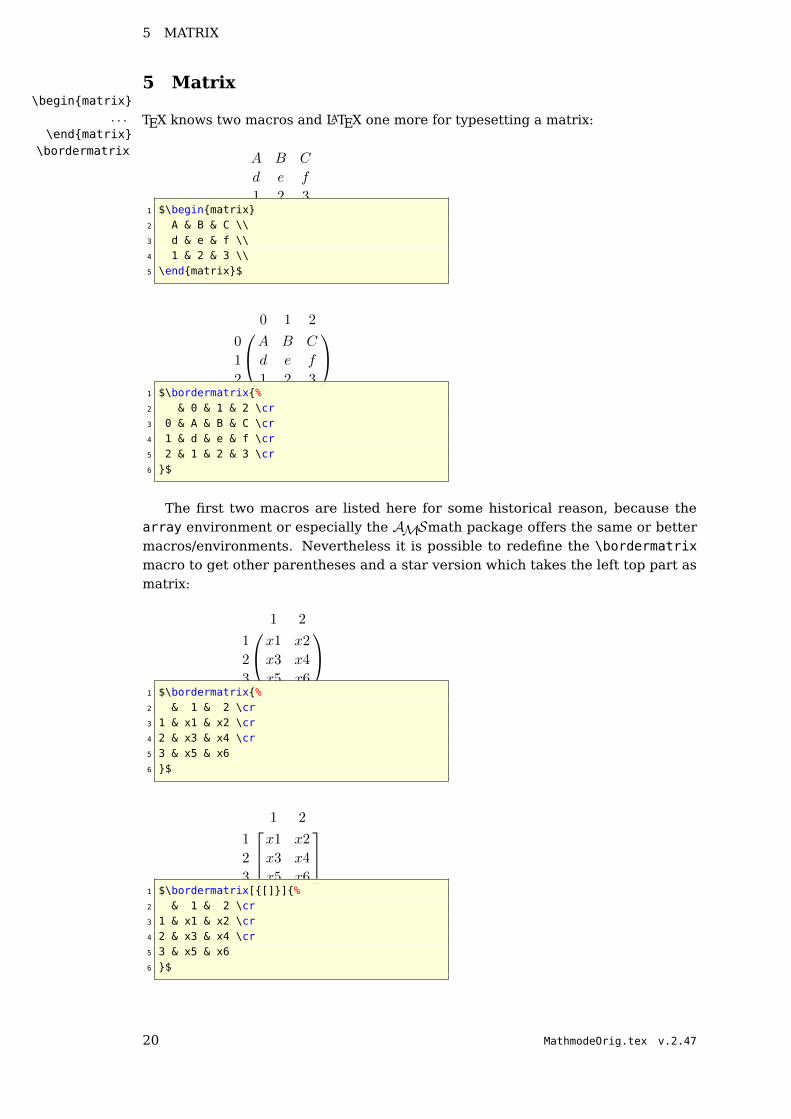
TEX knows two macros and LATEX one more for typesetting a matrix:

A B C

d e f

1 2 31 $\beginmatrix2 A & B & C \\3 d & e & f \\4 1 & 2 & 3 \\5 \endmatrix$

0 1 2

0 A B C

1 d e f

2 1 2 3

1 $\bordermatrix%2 & 0 & 1 & 2 \cr3 0 & A & B & C \cr4 1 & d & e & f \cr5 2 & 1 & 2 & 3 \cr6 $

The first two macros are listed here for some historical reason, because thearray environment or especially the AMSmath package offers the same or bettermacros/environments. Nevertheless it is possible to redefine the \bordermatrixmacro to get other parentheses and a star version which takes the left top part asmatrix:

1 2

1 x1 x2

2 x3 x4

3 x5 x6

1 $\bordermatrix%2 & 1 & 2 \cr3 1 & x1 & x2 \cr4 2 & x3 & x4 \cr5 3 & x5 & x66 $

1 2

1 x1 x2

2 x3 x4

3 x5 x6

1 $\bordermatrix[[]]%2 & 1 & 2 \cr3 1 & x1 & x2 \cr4 2 & x3 & x4 \cr5 3 & x5 & x66 $


5 MATRIX

1 2

1 x1 x2

2 x3 x4

3 x5 x6

1 $\bordermatrix[\\]%2 & 1 & 2 \cr3 1 & x1 & x2 \cr4 2 & x3 & x4 \cr5 3 & x5 & x66 $

x1 x2 1

x3 x4 2

x5 x6 3

1 2

1 $\bordermatrix*%2 x1 & x2 & 1 \cr3 x3 & x4 & 2 \cr4 x5 & x6 & 3 \cr5 1 & 26 $

x1 x2 1

x3 x4 2

x5 x6 3

1 2

1 $\bordermatrix*[[]]%2 x1 & x2 & 1 \cr3 x3 & x4 & 2 \cr4 x5 & x6 & 3 \cr5 1 & 26 $

x1 x2 1

x3 x4 2

x5 x6 3

1 2

1 $\bordermatrix*[\\]%2 x1 & x2 & 1 \cr3 x3 & x4 & 2 \cr4 x5 & x6 & 3 \cr5 1 & 26 $

There is now an optional argument for the parenthesis with () as the default one.To get such a behaviour, write into the preamble:

1 \makeatletter2 \newif\if@borderstar3 \def\bordermatrix\@ifnextchar*%4 \@borderstartrue\@bordermatrix@i\@borderstarfalse\@bordermatrix@i*%5 6 \def\@bordermatrix@i*\@ifnextchar[\@bordermatrix@ii\@bordermatrix@ii[()]7 \def\@bordermatrix@ii[#1]#2%8 \begingroup9 \m@th\@tempdima8.75\p@\setbox\z@\vbox%

10 \def\cr\crcr\noalign\kern 2\p@\global\let\cr\endline %


6 SUPER/SUBSCRIPT AND LIMITS

11 \ialign $##$\hfil\kern 2\p@\kern\@tempdima & \thinspace %12 \hfil $##$\hfil && \quad\hfil $##$\hfil\crcr\omit\strut %13 \hfil\crcr\noalign\kern -\baselineskip#2\crcr\omit %14 \strut\cr%15 \setbox\tw@\vbox\unvcopy\z@\global\setbox\@ne\lastbox%16 \setbox\tw@\hbox\unhbox\@ne\unskip\global\setbox\@ne\lastbox%17 \setbox\tw@\hbox%18 $\kern\wd\@ne\kern -\@tempdima\left\@firstoftwo#1%19 \if@borderstar\kern2pt\else\kern -\wd\@ne\fi%20 \global\setbox\@ne\vbox\box\@ne\if@borderstar\else\kern 2\p@\fi%21 \vcenter\if@borderstar\else\kern -\ht\@ne\fi%22 \unvbox\z@\kern-\if@borderstar2\fi\baselineskip%23 \if@borderstar\kern-2\@tempdima\kern2\p@\else\,\fi\right\@secondoftwo#1 $%24 \null \;\vbox\kern\ht\@ne\box\tw@%25 \endgroup26 27 \makeatother

The matrix environment macro cannot be used together with the AMSmathpackage, it redefines this environment (see section 26.6 on page 60).

6 Super/Subscript and limits

Writing amin and amax gives the same depth for the subscript, but writing them inupright mode with \mbox gives a different depth: amin and amax. The problem isthe different height, which can be modified in several ways

• $a_\mbox\vphantomimax$: amin and amax;

• $a_\mathrmmax$: amin and amax;

• $a_\max$: amin and amax. Both are predefined operators (see section 16 onpage 40).

6.1 Multiple limits\atop

For general information about limits read section 2.1 on page 9. With the TEXcommand \atop multiple limits for a \sum or \prod are possible. The syntax is:

above

below1 \[ above \atop below \]

which is nearly the same as a fraction without a rule. This can be enhanced toa\atop b\atop c and so on. For equation 21 do the following steps:

∑

1≤j≤p1≤j≤q1≤k≤r

aijbjkcki (21)

1 \beginequation\labeleq:atop2 \sum_1\le j\le p\atop %3 1\le j\le q\atop 1\le k\le r%4 a_ijb_jkc_ki5 \endequation


6.2 Problems 7 ROOTS

\shortstackwhich is not the best solution because the space between the lines is too big. The

AMSmath package provides several commands for limits (section 35 on page 66)and the \underset and \overset commands (see section 41 on page 73).

6.2 Problems∑


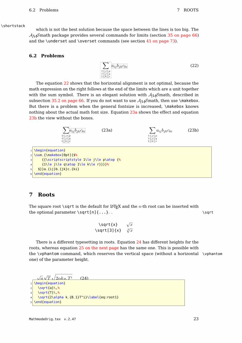
aijbjkcki (22)

The equation 22 shows that the horizontal alignment is not optimal, because themath expression on the right follows at the end of the limits which are a unit togetherwith the sum symbol. There is an elegant solution with AMSmath, described insubsection 35.2 on page 66. If you do not want to use AMSmath, then use \makebox.But there is a problem when the general fontsize is increased, \makebox knowsnothing about the actual math font size. Equation 23a shows the effect and equation23b the view without the boxes.

∑


aijbjkcki (23a)∑


aijbjkcki (23b)

1 \beginequation2 \sum_\makebox[0pt]$%3 \scriptscriptstyle 1\le j\le p\atop %4 1\le j\le q\atop 1\le k\le r%5 $a_ijb_jkc_ki6 \endequation

7 Roots

The square root \sqrt is the default for LATEX and the n-th root can be inserted withthe optional parameter \sqrt[n].... . \sqrt

\sqrtx√x

\sqrt[3]x 3√x

There is a different typesetting in roots. Equation 24 has different heights for theroots, whereas equation 25 on the next page has the same one. This is possible withthe \vphantom command, which reserves the vertical space (without a horizontal \vphantom

one) of the parameter height.

√a√T√

2αkB1Ti (24)

1 \beginequation2 \sqrta\,%3 \sqrtT\,%4 \sqrt2\alpha k_B_1T^i\labeleq:root15 \endequation


8 BRACKETS, BRACES . . .

√a

√T√

2αkB1Ti (25)

1 \beginequation\labeleq:root22 \sqrta\vphantomk_B_1Tî\,%3 \sqrtT\vphantomk_B_1Tî\,%4 \sqrt2\alpha k_B_1Tî5 \endequation

The typesetting looks much better, especially when the formula has differentroots in a row, like equation 24 on the preceding page. Using AMSmath with the\smash command9 gives some more possibilities for the typesetting of roots (seesection 30 on page 62).

8 Brackets, braces and parentheses

This is one of the major problems inside the math mode, because there is often aneed for different brackets, braces and parentheses in different size. At first we hadto admit, that there is a difference between the characters “()[]/\ | ‖ bc de 〈〉↑⇑ ↓⇓ lm” and their use as an argument of the \left and \right command, where\leftX

\rightX LATEX stretches the size in a way that everything between the pair of left and rightparentheses is smaller than the parentheses themselves. In some cases10 it may beuseful to choose a fixed height, which is possible with the \big-series. Instead ofwriting \leftX or \rightX one of the following commands can be chosen:

\bigX\BigX

\biggX\BiggX

default ()[]/\|‖ bc de 〈〉 ↑⇑ ↓⇓lm\bigX

() [] /∖ ∣∣ ∥∥ ⌊⌋ ⌈⌉ ⟨⟩ x~w yw xy~

\BigX() [] /∖ ∣∣∣

∥∥∥⌊⌋ ⌈⌉ ⟨⟩ x

~wwywwxy~w

\biggX

() [] /∖∣∣∣∣∥∥∥∥⌊⌋ ⌈⌉ ⟨⟩ x

~wwwywwwxy~ww

\BiggX

() []/∖ ∣∣∣∣∣

∥∥∥∥∥

⌊⌋ ⌈⌉ ⟨⟩ x

~wwww

y

wwww

xy

~wwwOnly a few commands can be written in a short form like \big(. The “X” has to

be replaced with one of the following characters or commands from table 3 on thenext page, which shows the parentheses character, its code for the use with one ofthe “big” commands and an example with the code for that.\biglX

\bigrX For all commands there exists a left/right version \bigl, \bigr, \Bigl and so on,which only makes sense when writing things like:

9The \smash command exists also in LATEX but without an optional argument, which makes the usefor roots possible.

10See section 8.1.1 on page 27 for example.



)×ab×(

(26)

)× a

b×(

(27)

1 \beginalign2 \biggl)\times \fracab \times\biggr(3 \endalign4 \beginalign5 \bigg)\times \fracab \times\bigg(6 \endalign

LATEX takes the \biggl) as a mathopen symbol, which has by default anotherhorizontal spacing.

In addition to the above commands there exist some more: \bigm, \Bigm, \biggmand \Biggm, which work as the standard ones (without the addtional “m”) but addsome more horizontal space between the delimiter and the formula before and after \bigmX

\bigmX(see table 2).

Table 2: Difference between the default \bigg and the \biggm command

(1

3

∣∣∣∣3

4

)

1 $\bigg(\displaystyle\frac13\bigg|\frac34\bigg)$

(1

3

∣∣∣∣3

4

)

1 $\bigg(\displaystyle\frac13\biggm|\frac34\bigg)$

Table 3: Use of the different parentheses for the “big”commands

Char Code Example Code

( ) ( ) 3(a2 + bc

2)

3\Big( aˆ2+bˆcˆ2\Big)

[ ] [ ] 3[a2 + bc

2]

3\Big[ aˆ2+bˆcˆ2\Big]

/ \ /\backslash 3/a2 + bc

2∖

3\Big/aˆ2+bˆcˆ2\Big\backslash

\\ 3a2 + bc

2

3\Big\ aˆ2+bˆcˆ2\Big\

| ‖ | \Vert 3∣∣∣a2 + bc

2∥∥∥ 3\Big|aˆ2+bˆcˆ2\Big\Vert

b c \lfloor\rfloor

3⌊a2 + bc

2⌋

3\Big\lfloor aˆ2+bˆcˆ2\Big\rfloor

d e \lceil\rceil 3⌈a2 + bc

2⌉

3\Big\lceil aˆ2+bˆcˆ2\Big\rceil



Char Code Example Code

〈〉 \langle\rangle3⟨a2 + bc

2⟩

3\Big\langleaˆ2+bˆcˆ2\Big\rangle

↑ ⇑ \uparrow\Uparrow

3xa2 + bc

2~ww 3\Big\uparrow

aˆ2+bˆcˆ2\Big\Uparrow

↓ ⇓ \downarrow\Downarrow

3ya2 + bc

2ww 3\Big\downarrow aˆ2+bˆcˆ2

\Big\Downarrow

l m \updownarrow\Updownarrow

3xya2 + bc

2~w 3\Big\updownarrow

aˆ2+bˆcˆ2\Big\Updownarrow


8.1 Examples 8 BRACKETS, BRACES . . .

8.1 Examples

8.1.1 Braces over several lines

The following equation in the single line mode looks like

1

2∆(fijf

ij) = 2

∑

i<j

χij(σi − σj)2 + f ij∇j∇i(∆f) +∇kfij∇kf ij + f ijfk[2∇iRjk −∇kRij ]

(28)and is too long for the text width and the equation number has to be placed underthe equation.11 With the array environment the formula can be split in two smallerpieces:

12∆(fijf

ij) = 2

∑

i<j

χij(σi − σj)2 + f ij∇j∇i(∆f)+

+∇kfij∇kf ij + f ijfk[2∇iRjk −∇kRij ])

(29)

It is obvious that there is a problem with the right closing parentheses. Becauseof the two pairs “\left( ... \right.” and “\left. ... \right)” they have adifferent size because every pair does it in its own way. Using the Bigg commandchanges this into a better typesetting:

12∆(fijf

ij) = 2

(∑

i<j


+∇kfij∇kf ij + f ijfk[2∇iRjk −∇kRij ]) (30)

1 \arraycolsep=2pt2 \beginequation3 \beginarrayrcl4 \frac12\Delta(f_ijfîj) & = & 2\Bigg(\displaystyle5 \sum_i<j\chi_ij(\sigma_i-\sigma_j)^2+fîj%6 \nabla_j\nabla_i(\Delta f)+\\7 & & +\nabla_kf_ij\nabla^kfîj+fîjf^k[28 \nabla_iR_jk-\nabla_kR_ij]\Bigg)9 \endarray

10 \endequation11

Section 26.3.1 on page 55 shows another solution for getting the right size forparentheses when breaking the equation in smaller pieces.

B(r, φ, λ) =µ

r

[ ∞∑

n=2

((Rer

)nJnPn(sφ)

+

n∑

m=1

(Rer

)n(Cnm cosmλ+ Snm sinmλ)Pnm(sφ)

)]

11In standard LATEX the equation and the number are printed one over the other for too long formulas.Only AMSmath puts it one line over (left numbers) or under (right numbers) the formula.


8 BRACKETS, BRACES . . . 8.2 New delimiters

1 \beginalign*2 B(r,\phi,\lambda) = & \,\dfrac\mur3 \Bigg[\sum_n=2^\infty \Bigg( \left( \dfracR_er \right)^n J_nP_n(s\phi) \\4 & +\sum_m=1^n \left( \dfracR_er \right) ^n5 (C_nm\cos m\lambda+S_nm\sin m\lambda)P_nm(s\phi) \Bigg)\Bigg]6 \endalign*

8.1.2 Middle bar

See section 47.6 on page 92 for examples and the use of package braket.

8.2 New delimiters

The default delimiters are defined in the file fontmath.ltx which is stored in gen-eral in [TEXMF]/tex/latex/base/fontmath.ltx. If we need for example a thickervertical symbol than the existing \vert symbol we can define in the preamble:

1 \DeclareMathDelimiter\Norm2 \mathordlargesymbols"3Elargesymbols"3E

The character number 3E16 (decimal 62) from the cmex10 font is the small thickvertical rule. Now the new delimiter \Norm can be used in the usual way:

∗BLA∗∗BLA∗∗BLUB∗

1 $\left\Norm *BLA* \right\Norm$2

3 $\left\Norm \dfrac*BLA**BLUB* \right\Norm$

8.3 Problems with parentheses\delimitershortfall\delimiterfactor It is obvious that the following equation has not the right size of the parenthesis in

the second integral, the inner one should be a bit smaller than the outer one.

ˆγF ′(z)dz =

ˆ β

αF ′ (γ(t)) · γ′(t)dt

1 \[2 \int_\gamma F’(z) dz =\int_\alpha^\beta3 F’\left(\gamma (t)\right)\cdot\gamma ’(t)dt4 \]

The problem is that TEX controlls the height of the parenthesis with \delimitershortfalland \delimiterfactor, with the default values

\delimitershortfall=5pt\delimiterfactor=901

\delimiterfactor/1000 is the relative size of the parenthesis for a given formulaenvironment. They could be of \delimitershortfall too short. These values arevalid at the end of the formula, the best way is to set them straight before the mathenvironment or globally for all in the preamble.


10 FONT COMMANDS

ˆγF ′(z)dz =

ˆ β

αF ′(γ(t)

)· γ′(t)dt

1 \delimitershortfall=-1pt2 \[3 \int_\gamma F’(z) dz =\int_\alpha^\beta4 F’\left(\gamma (t)\right)\cdot\gamma ’(t)dt5 \]

9 Text in math mode

Standard text in math mode should be written in upright shape and not in the italicone. This shape is reserved for the variable names: I am text inside math. (see alsoTable 7 on page 31). There are different ways to write text inside math. \textstyle

\mbox\mathrm• \mathrm. It is like math mode (no spaces), but in upright mode

• \textrm. Upright mode with printed spaces (real textmode)

• \mbox. The font size is still the one from \textstyle (see section 12 on page 36),so that you have to place additional commands when you use \mbox in a super-or subscript for limits.

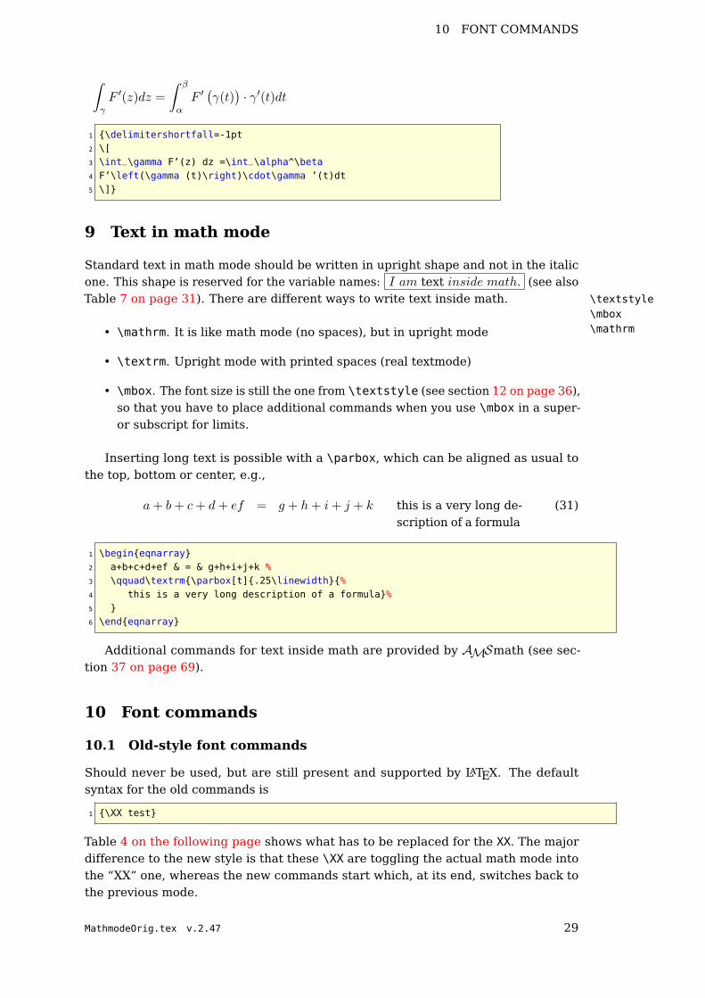
Inserting long text is possible with a \parbox, which can be aligned as usual tothe top, bottom or center, e.g.,

a+ b+ c+ d+ ef = g + h+ i+ j + k this is a very long de-scription of a formula

(31)

1 \begineqnarray2 a+b+c+d+ef & = & g+h+i+j+k %3 \qquad\textrm\parbox[t].25\linewidth%4 this is a very long description of a formula%5 6 \endeqnarray

Additional commands for text inside math are provided by AMSmath (see sec-tion 37 on page 69).

10 Font commands

10.1 Old-style font commands

Should never be used, but are still present and supported by LATEX. The defaultsyntax for the old commands is

1 \XX test

Table 4 on the following page shows what has to be replaced for the XX. The majordifference to the new style is that these \XX are toggling the actual math mode intothe “XX” one, whereas the new commands start which, at its end, switches back tothe previous mode.


11 SPACE 10.2 New-style font commands

\bf test \cal T EST \it test \rm test \tt test

Table 4: Old font style commands

10.2 New-style font commands\mathrm\mathfrak\mathcal\mathsf\mathbb\mathtt\mathit\mathbf

The default syntax is

1 \mathXXtest

Table 5 shows what has to be replaced for the XX. See section 47.13 on page 98 foradditional packages.

Table 5: Fonts in math modeCommand Testdefault ABCDEFGHIJKLMNOPQRSTUV WXY Z

abcdefghijklmnopqrstuvwxyz\mathfrak ABCDEFGHIJKLMNOPQRSTUVWXYZ

abcdefghijklmnopqrstuvwxyz

\mathcala ABCDEFGHIJ KLMNOPQRST UVWXYZ\mathsf ABCDEFGHIJKLMNOPQRSTUVWXYZ

abcdefghijklmnopqrstuvwxyz\mathbba ABCDEFGHIJKLMNOPQRSTUVWXYZ\mathtt ABCDEFGHIJKLMNOPQRSTUVWXYZ

abcdefghijklmnopqrstuvwxyz\mathit ABCDEFGHIJKLMNOPQRSTUVWXYZ

abcdefghijklmnopqrstuvwxyz\mathrm ABCDEFGHIJKLMNOPQRSTUVWXYZ

abcdefghijklmnopqrstuvwxyz\mathbf ABCDEFGHIJKLMNOPQRSTUVWXYZ

abcdefghijklmnopqrstuvwxyz\mathdsb ABCDEFGHIJKLMNOPQRSTUVWXYZ

aNot available for lower letters. For mathcal exists a non free font for lower letters(http://www.pctex.com)

bNeeds package dsfont

11 Space

11.1 Math typesetting\thinmuskip\medmuskip

\thickmuskip

LATEX defines the three math lengths12 with the following values13:

1 \thinmuskip=3mu2 \medmuskip=4mu plus 2mu minus 4mu3 \thickmuskip=5mu plus 5mu

where mu is the abbreviation for math unit.

1mu =1

18em

12For more information see: http://www.tug.org/utilities/plain/cseq.html13see fontmath.ltx


http://www.tug.org/utilities/plain/cseq.html

11.2 Additional horizontal spacing 11 SPACE

default f(x) = x2 + 3x0 · sinx\thinmuskip=0mu f(x) = x2 + 3x0 · sinx\medmuskip=0mu f(x) = x2+3x0·sinx\thickmuskip=0mu f(x)=x2 + 3x0 · sinxall set to zero f(x)=x2+3x0·sinx

Table 6: The meaning of the math spaces

These lengths can have all glue and are used for the horizontal spacing in mathexpressions where TEX puts spaces between symbols and operators. The meaning ofthese different horizontal skips is shown in table 6. For a better typesetting LATEXinserts different spaces between the symbols.

\thinmuskip space between ordinary and operator atoms

\medmuskip space between ordinary and binary atoms in display and text styles

\thickmuskip space between ordinary and relation atoms in display and text styles

11.2 Additional horizontal spacing\thinspace\medspace\thickspace\negthinspace\negmedspace\negthickspace

Positive Space Negative Space

$ab$ a b

$a b$ a b

$a\ b$ a b

$a\mbox\textvisiblespaceb$ a b

$a\,b$ ($a\thinspace b$) a b $a\! b$ a b

$a\: b$ ($a\medspace b$) a b $a\negmedspace b$ a b

$a\; b$ ($a\thickspace b$ a b $a\negthickspace b$ a b

$a\quad b$ a b

$a\qquad b$ a b

$a\hspace0.5cmb$ a b $a\hspace-0.5cmb$ ab

$a\kern0.5cm b$ a b $a\kern-0.5cm b$ ab

$a\hphantomxxb$ a b

$axxb$ a xx b

Table 7: Spaces in math mode

LaTeX defines the following short commands:

\def\>\mskip\medmuskip\def\;\mskip\thickmuskip\def\!\mskip-\thinmuskip

In math mode there is often a need for additional tiny spaces between variables, e.g.,

Ldi

dtwritten with a tiny space between L and

di

dtlooks nicer: L

di

dt. Table 7 shows

a list of all commands for horizontal space which can be used in math mode. The


11 SPACE 11.3 Problems

“space” is seen “between” the boxed a and b. For all examples a is \boxeda andb is \boxedb. The short forms for some spaces may cause problems with other\hspace

\hphantom\kern

packages. In this case use the long form of the commands.

11.3 Problems

Using \hphantom in mathmode depends to on object. \hphantom reserves only thespace of the exact width without any additional space. In the following examplethe second line is wrong: & \hphantom\rightarrow b\\. It does not reserve anyadditional space.

a→ b

b

b

b1 \beginalign*2 a & \rightarrow b\\3 & \hphantom\rightarrow b\\4 & \mkern\thickmuskip\hphantom\rightarrow\mkern\thickmuskip b\\5 & \mathrel\hphantom\rightarrow b6 \endalign*

This only works when the math symbol is a mathrel one, otherwise you have tochange the horizontal space to \medmuskip or \thinmuskip or to use an empty groupafter the \hphantom command. For more informations about the math objects lookinto fontmath.ltx or amssymb or use the \show macro, which prints out the type ofthe mathsymbol, e.g., \show\rightarrow with the output:

1 > \rightarrow=\mathchar"3221.2 l.20 \show\rightarrow

The first digit represents the type:0 : ordinary1 : large operator2 : binary operation3 : relation4 : opening5 : closing6 : punctuation7 : variable family

Grouping a math symbol can change the behaviour in horizontal spacing. Compare50 × 1012 and 50×1012, the first one is typeset with $50\times10^12$ and thesecond one with $50\times10^12$. Another possibilty is to use the numprintpackage.14

11.4 Dot versus comma\mathpunct

\mathord In difference to a decimal point and a comma as a marker of thousands a lot ofcountries prefer it vice versa. To get the same behaviour the meaning of dot andcomma has to be changed:

14CTAN://macros/latex/contrib/numprint/


ftp://ftp.dante.de/tex-archive/macros/latex/contrib/numprint/

11.5 Vertical whitespace 11 SPACE

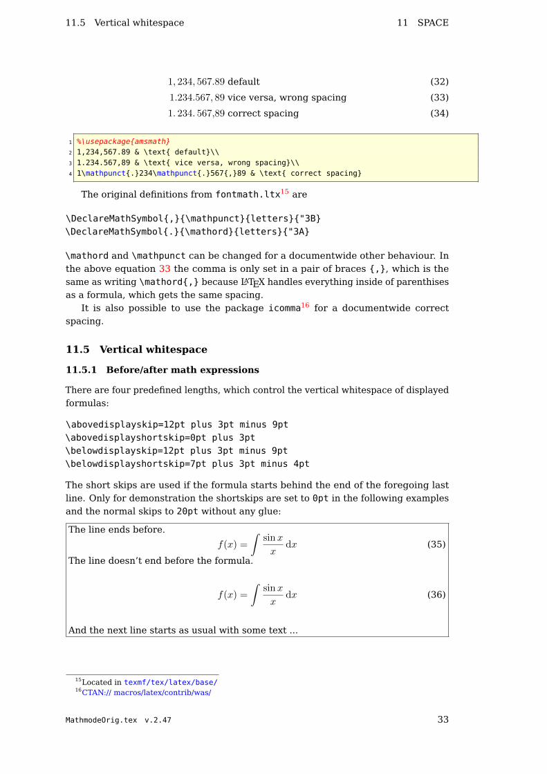
1, 234, 567.89 default (32)

1.234.567, 89 vice versa, wrong spacing (33)

1. 234. 567,89 correct spacing (34)

1 %\usepackageamsmath2 1,234,567.89 & \text default\\3 1.234.567,89 & \text vice versa, wrong spacing\\4 1\mathpunct.234\mathpunct.567,89 & \text correct spacing

The original definitions from fontmath.ltx15 are

\DeclareMathSymbol,\mathpunctletters"3B\DeclareMathSymbol.\mathordletters"3A

\mathord and \mathpunct can be changed for a documentwide other behaviour. Inthe above equation 33 the comma is only set in a pair of braces ,, which is thesame as writing \mathord, because LATEX handles everything inside of parenthisesas a formula, which gets the same spacing.

It is also possible to use the package icomma16 for a documentwide correctspacing.

11.5 Vertical whitespace

11.5.1 Before/after math expressions

There are four predefined lengths, which control the vertical whitespace of displayedformulas:

\abovedisplayskip=12pt plus 3pt minus 9pt\abovedisplayshortskip=0pt plus 3pt\belowdisplayskip=12pt plus 3pt minus 9pt\belowdisplayshortskip=7pt plus 3pt minus 4pt

The short skips are used if the formula starts behind the end of the foregoing lastline. Only for demonstration the shortskips are set to 0pt in the following examplesand the normal skips to 20pt without any glue:

The line ends before.

f(x) =

ˆsinx

xdx (35)

The line doesn’t end before the formula.

f(x) =

ˆsinx

xdx (36)

And the next line starts as usual with some text ...

15Located in texmf/tex/latex/base/16CTAN:// macros/latex/contrib/was/


texmf/tex/latex/base/

ftp://ftp.dante.de/tex-archive/macros/latex/contrib/was/

11 SPACE 11.5 Vertical whitespace

1 \abovedisplayshortskip=0pt2 \belowdisplayshortskip=0pt3 \abovedisplayskip=20pt4 \belowdisplayskip=20pt5 \noindent The line ends before.6 \beginequation7 f(x) = \int\frac\sin xx\,\mathrmdx8 \endequation9 \noindent The line doesn’t end before the formula.

10 \beginequation11 f(x) = \int\frac\sin xx\,\mathrmdx12 \endequation13 \noindent And the next line starts as usual with some text ...

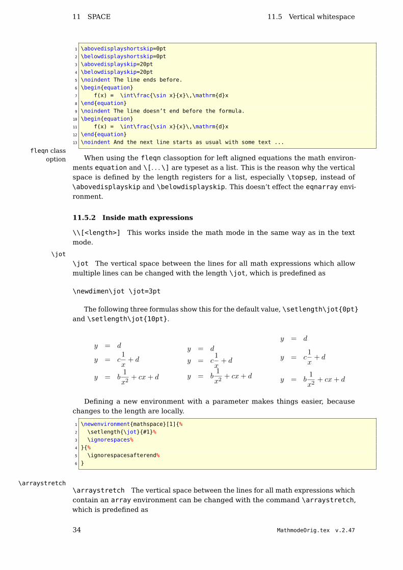
fleqn classoption When using the fleqn classoption for left aligned equations the math environ-

ments equation and \[. . . \] are typeset as a list. This is the reason why the verticalspace is defined by the length registers for a list, especially \topsep, instead of\abovedisplayskip and \belowdisplayskip. This doesn’t effect the eqnarray envi-ronment.

11.5.2 Inside math expressions

\\[<length>] This works inside the math mode in the same way as in the textmode.

\jot

\jot The vertical space between the lines for all math expressions which allowmultiple lines can be changed with the length \jot, which is predefined as

\newdimen\jot \jot=3pt

The following three formulas show this for the default value, \setlength\jot0ptand \setlength\jot10pt.

y = d

y = c1

x+ d

y = b1

x2+ cx+ d

y = d

y = c1

x+ d

y = b1

x2+ cx+ d

y = d

y = c1

x+ d

y = b1

x2+ cx+ d

Defining a new environment with a parameter makes things easier, becausechanges to the length are locally.

1 \newenvironmentmathspace[1]%2 \setlength\jot#1%3 \ignorespaces%4 %5 \ignorespacesafterend%6

\arraystretch\arraystretch The vertical space between the lines for all math expressions whichcontain an array environment can be changed with the command \arraystretch,which is predefined as


11.5 Vertical whitespace 11 SPACE

\renewcommand\arraystretch1

Renewing this definition is global to all following math expressions, so it shouldbe used in the same way as \jot.

\vskip Another spacing for single lines is possible with the \vskip macro:

0 1 1 0 0 1

1 0 0 1 1 0

0 1 1 01√2

1

1 0 1 0 1 0

0 1 0 1 0 1

1 \[2 \beginpmatrix3 0 & 1 & 1 & 0 & 0 & 1 \\4 1 & 0 & 0 & 1 & 1 & 0 \\5 \noalign\vskip2pt6 0 & 1 & 1 & 0 & \dfrac1\sqrt2 & 1\\7 \noalign\vskip2pt8 1 & 0 & 1 & 0 & 1 & 0 \\9 0 & 1 & 0 & 1 & 0 & 1 \\

10 \endpmatrix11 \]

Package setspace To have all formulas with another vertical spacing, one canchoose the package setspace and redefining some of the math macros, e.g.,

1 \newcommand*\Array[2][1]\setstretch#1\array#22 \let\endArray\endarray

a = b

a = b

a = b

texta = ba = ba = b

text

1 \[2 \beginArray[2]cc3 a =&b\\4 a =&b\\5 a =&b6 \endArray7 \]8

9 text $\beginArraycc10 a =&b\\11 a =&b\\12 a =&b13 \endArray$ text


12 STYLES

12 Styles

Mode Inline Displayed

default f(t) = T2π

´1

sin ωtdt f(t) =

T

2π

ˆ1

sin ωt

dt

\displaystyle f(t) =T

2π

ˆ1

sin ωt

dt f(t) =T

2π

ˆ1

sin ωt

dt

\scriptstyle f(t) = T2π

´1

sin ωtdt

f(t)= T2π

´1

sin ωtdt

\scriptscriptstyle f(t)= T2π

´ 1sin ωt

dtf(t)= T

2π

´ 1sin ωt

dt

\textstyle f(t) = T2π

´1

sin ωtdt

f(t) = T2π

´1

sin ωtdt

Table 8: Math styles

This depends on the environment in which they are used. An inline formulahas a default math fontsize called \textstyle, which is smaller than the one for\textstyle

\displaystyle\scriptstyle

\scripscriptstyle

a display formula (see section 3), which is called \displaystyle. Beside thispredefinition there are two other special fontstyles for math, \scriptstyle and\scriptscriptstyle. They are called “style” in difference to “size”, because theyhave a dynamic character, their real fontsize belongs to the environment in whichthey are used. A fraction for example is by default in scriptstyle when it is in an inline

formula like this ab , which can be changed to

a

b. This may be in some cases useful

but it looks in general ugly because the line spacing is too big. These four styles arepredefined and together in a logical relationship. It is no problem to use the otherstyles like large, \Large, . . . outside the math environment. For example a fraction

written with \Huge:ab (\Huge$\fracab$). This may cause some problems when

you want to write a displayed formula in another fontsize, because it also affects theinterline spacing of the preceding part of the paragraph. If you end the paragraph,you get problems with spacing and page breaking above the equations. So it is betterto declare the font size and then restore the baselines:

ˆ 2

1

1

x2dx = 0.5 (37)

1 \makeatletter2 \newenvironmentsmallequation[1]%3 \skip@=\baselineskip4 #1%5 \baselineskip=\skip@6 \equation7 \endequation \ignorespacesafterend8 \makeatother9

10 \beginsmallequation\tiny11 \int_1^2\,\frac1x^2\,\mathrmdx=0.512 \endsmallequation

If you use this the other way round for huge fontsizes, don’t forget to load package


14 ACCENTS

exscale (see section 47.14 on page 98). Also see this section for diffent symbol sizes.

13 Dots\cdots\dots\dotsb\dotsc\dotsi\dotsm\dotso\ldots\vdots

In addition to the above decorations there are some more different dots which aresingle commands and not by default over/under a letter. It is not easy to see thedifferences between some of them. Dots from lower left to upper right are possible

with \reflectbox$\ddots$...

\cdots · · · \ddots. . . \dotsb · · · \dotsc . . . \dotsi · · ·

\dotsm · · · \dotso . . . \ldots . . . \vdots...

Table 9: Dots in math mode

14 Accents

The letter “a” is only for demonstration. The table 10 shows all in standard LATEXavailable accents and also the ones placed under a character. With package amssymbit is easy to define new accents. For more information see section 31 on page 63 orother possibilities at section 47.1 on page 90.

\acute a \bar a \breve a\bar a \breve a

\check a \dddot...a \ddot a

\dot a \grave a \hat a

\mathring a \overbrace︷︸︸︷a \overleftarrow ←−a

\overleftrightarrow ←→a \overline a \overrightarrow −→a\tilde a \underbar a \underbrace a︸︷︷︸

\underleftarrow a←− \underleftrightarrow a←→ \underline a

\underrightarrow a−→ \vec ~a \widehat a

\widetilde a

Table 10: Accents in math mode

The letters i and j can be substituted with the macros \imath and \jmathwhen an accents is placed over these letters and the dot should disappear: ~ı

...

($\vec\imath\ \dddot\jmath$).

Accents can be used in different ways, e.g., strike a single character with ahorizontal line like $\mathaccent‘-A$: -A or $\mathaccent\mathcode‘-A$: −A. Insection 47.7 on page 94 is a better solution for more than one character.

14.1 Over- and underbrackets

There are no \underbracket and \overbracket commands in the list of accents.They can be defined in the preamble with the following code.

1 \makeatletter2 \def\underbracket%3 \@ifnextchar[\@underbracket\@underbracket [\@bracketheight]%4


14 ACCENTS 14.1 Over- and underbrackets

5 \def\@underbracket[#1]%6 \@ifnextchar[\@under@bracket[#1]\@under@bracket[#1][0.4em]%7 8 \def\@under@bracket[#1][#2]#3%\message Underbracket: #1,#2,#39 \mathop\vtop\m@th \ialign ##\crcr $\hfil \displaystyle #3\hfil $%

10 \crcr \noalign \kern 3\p@ \nointerlineskip \upbracketfill #1#211 \crcr \noalign \kern 3\p@ \limits12 \def\upbracketfill#1#2$\m@th \setbox \z@ \hbox $\braceld$13 \edef\@bracketheight\the\ht\z@\bracketend#1#214 \leaders \vrule \@height #1 \@depth \z@ \hfill15 \leaders \vrule \@height #1 \@depth \z@ \hfill \bracketend#1#2$16 \def\bracketend#1#2\vrule height #2 width #1\relax17 \makeatother

1. \underbrace... is an often used command:

x2 + 2x+ 1︸︷︷︸ = f(x) (38)

(x+ 1)2

2. Sometimes an underbracket is needed, which can be used in more ways than\underbrace.... An example for \underbracket...:

Hate Science 1→ 2→ 3→ 4→ 5→ 6→ 7→ 8→ 9→ 10 Love Science

low medium high

14.1.1 Use of \underbracket...

The \underbracket... command has two optional parameters:

• the line thickness in any valid latex unit, e.g., 1pt

• the height of the edge brackets, e.g., 1em

using without any parameters gives the same values for thickness and height aspredefined for the \underbrace command.

1. $\underbracketfoo~bar$ foo bar

2. $\underbracket[2pt]foo~bar$ foo bar

3. $\underbracket[2pt][1em] foo~bar$ foo bar

14.1.2 Overbracket

In addition to the underbracket an overbracket is also useful, which can be used inmore ways than \overbrace.... For example:

Hate Science 1→ 2→ 3→ 4→ 5→ 6→ 7→ 8→ 9→ 10 Love Science

low medium high


14.2 Vectors 15 EXPONENTS AND INDICES

The \overbracket... command has two optional parameters:

• the line thickness in any valid latex unit, e.g., 1pt

• the height of the edge brackets, e.g., 1em

using without any parameters gives the same values for thickness and height aspredefined for the \overbrace command.

1. $\overbracket foo\ bar$ foo bar

2. $\overbracket[2pt] foo\ bar$ foo bar

3. $\overbracket[2pt] [1em] foo\ bar$ foo bar

14.2 Vectors

Especially for vectors there is the package esvect17 package, which looks betterthan the \overrightarrow, e.g.,

\vv... \overrightarrow...#»a −→a

# »

abc−→abc

#»ı −→ı#»

Ax−→Ax

Table 11: Vectors with package esvect (in the right column the default one fromLATEX)

Look into the documentation for more details about the package esvect.

15 Exponents and indices

The two active characters _ and ^ can only be used in math mode. The followingcharacter will be printed as an index ($y=a_1x+a_0$: y = a1x+ a0) or as an exponent($x^2+y^2=r^2$: x2 + y2 = r2). For more than the next character put it inside of ,like $a_i-1+a_i+1<a_i$: ai−1 + ai+1 < ai.

Especially for multiple exponents there are several possibilities. For example:

((x2)3)4 = ((x2)3)4

=((x2)3)4

(39)

1 ((x^2)^3)^4 =2 ((x^2)^3)^4 =3 \left(\left(x^2\right)^3\right)^4

For variables with both exponent and indice index the order is not important,$a_1^2$ is exactly the same than $a^2_1$: a2

1 = a21. By default all exponents and

indices are set as italic characters. It is possible to change this behaviour to getupright characters. The following example shows this for the indices.

17CTAN://macros/latex/contrib/esvect/


http://www.ctan.org/tex-archive/macros/latex/contrib/esvect/

16 OPERATORS

Aabc123defabcxyz123defaa

Aabc123defabcxyz123defaa

1 $A_abc_xyz123def^abc123defaa$2

3 \makeatletter4 \catcode‘\_\active5 \def_#1\sb\operator@font#16 \makeatother7

8 $A_abc_xyz123def^abc123defaa$

16 Operators

They are written in upright font shape and are placed with some additional spacebefore and after for a better typesetting. With the AMSmath package it is possibleto define one’s own operators (see section 36 on page 68). Table 12 and 13 show alist of the predefined ones for standard LATEX.

\coprod∐

\bigvee∨

\bigwedge∧

\biguplus⊎

\bigcap⋂

\bigcup⋃

\intop´

\int´

\prod∏

\sum∑

\bigotimes⊗

\bigoplus⊕

\bigodot⊙

\ointop¸

\oint¸

\bigsqcup⊔

\smallint ∫

Table 12: The predefined operators of fontmath.ltx

The difference between \intop and \int is that the first one has by defaultover/under limits and the second subscript/superscript limits. Both can be changedwith the \limits or \nolimits command. The same behaviour happens to the\ointop and \oint Symbols.

\log log \lg lg \ln ln\lim lim \limsup lim sup \liminf lim inf\sin sin \arcsin arcsin \sinh sinh\cos cos \arccos arccos \cosh cosh\tan tan \arctan arctan \tanh tanh\cot cot \coth coth \sec sec\csc csc \max max \min min\sup sup \inf inf \arg arg\ker ker \dim dim \hom hom\det det \exp exp \Pr Pr\gcd gcd \deg deg \bmod mod\pmoda (mod a)

Table 13: The predefined operators of latex.ltx

For more predefined operator names see table 20 on page 91. It is easy to definea new operator with

1 \makeatletter2 \newcommand\foo\mathop\operator@font foo\nolimits3 \makeatother

Now you can use \foo in the usual way:


17 GREEK LETTERS

foo21 = x2

1 \[ \foo_1^2 = x^2 \]

In this example \foo is defined with \nolimits, means that limits are placed insuperscript/subscript mode and not over under. This is still possible with \limits inthe definition or the equation:

2foo

1= x2

1 \[ \foo\limits_1^2 = x^2 \]

AMSmath has an own macro for a definition, have a look at section 36 on page 68.

17 Greek letters

The AMSmath package simulates a bold font for the greek letters, it writes a greekcharacter twice with a small kerning. The \mathbf<character> doesn’t work withlower greek character. See section 40 on page 72 for the \pmb macro, which makes itpossible to print bold lower greek letters. Not all upper case letters have own macronames. If there is no difference to the roman font, then the default letter is used,e.g., A for the upper case of α. Table 14 shows only those upper case letters whichhave own macro names. Some of the lower case letters have an additional var optionfor an alternative.

lower default upper default \mathbf \mathit

\alpha α

\beta β

\gamma γ \Gamma Γ Γ Γ

\delta δ \Delta ∆ ∆ ∆

\epsilon ε

\varepsilon ε

\zeta ζ

\eta η

\theta θ \Theta Θ Θ Θ

\vartheta ϑ

\iota ι

\kappa κ

\lambda λ \Lambda Λ Λ Λ

\mu µ

\nu ν

\xi ξ \Xi Ξ Ξ Ξ

\pi π \Pi Π Π Π

\varpi $

\rho ρ

\varrho %

\sigma σ \Sigma Σ Σ Σ

\varsigma ς

\tau τ

\upsilon υ \Upsilon Υ Υ Υ

\phi φ \Phi Φ Φ Φ


19 \STACKREL

lower default upper default \mathbf \mathit

\varphi ϕ

\chi χ

\psi ψ \Psi Ψ Ψ Ψ

\omega ω \Omega Ω Ω Ω

Table 14: The greek letters

Bold greek letters are possible with the package bm (see section 47.5 on page 92)and if they should also be upright with the package upgreek:

$\bm\upalpha, \bm\upbeta ... $ α,β...

A useful definition maybe:

1 \usepackageupgreek2 \makeatletter3 \newcommand\bfgreek[1]\bm\@nameuseup#14 \makeatother

Then $\bfgreekmu$ will allow you to type µ to obtain an upright boldface µ.

18 Pagebreaks\allowdisplaybreaks

By default a displayed formula cannot have a pagebreak. This makes some sense,but sometimes it gives a better typesetting when a pagebreak is possible.

\allowdisplaybreaks

\allowdisplaybreaks enables TEX to insert pagebreaks into displayed formulaswhenever a newline command appears. With the command \displaybreak it is alsopossible to insert a pagebreak at any place.

19 \stackrel

\stackrel puts a character on top of another one which may be important if a usedsymbol is not predefined. For example “

∧=” (\stackrel\wedge=). The syntax is\stackrel

1 \stackreltopbase

Such symbols may be often needed so that a macro definition in the preamblemakes some sense:

1 \newcommand\eqdef%2 \ensuremath\mathrel\stackrel\mathrmdef=

With the \ensuremath command we can use the new \eqdef command in text and inmath mode, LATEX switches automatically in math mode, which saves some keystrokeslike the following command, which is written without the delimiters ($...$) for the

math modedef= , only \eqdef with a space at the end. In math mode together with

another material it may look like ~xdef= (x1, . . . , xn) and as command sequence

1 $\vecx\eqdef\left(x_1,\ldots,x_n\right)$

The fontsize of the top is one size smaller than the one from the base, but it is noproblem to get both the same size, just increase the top or decrease the base.


22 BOLDMATH

20 \choose

\choose is like \atop with delimiters or like \frac without the fraction line and alsowith delimiters. It is often used for binomial coefficients and has the following syntax: \choose

1 above \choose below

The two braces are not really important but it is safe to use them.

(m+ 1

n

)=

(m

n

)+

(m

k − 1

)(40)

1 m+1 \choose n=m \choose n+m \choose k-1\labeleq:choose

See section 29.2 on page 62 for the AMSmath equivalents and enhancements.

21 Color in math expressions

There is no difference in using colored text and colored math expressions. With

\usepackagecolor

in the preamble the macro \textcolor<color><text or math> exists.

f(x) =

∞

1

1

x2dx = 1 (41)

\textcolor

1 \beginequation2 \textcolorbluef(x) = \int\limits_1^\infty\textcolorred\frac1x^2\,\mathrmd

x=13 \endequation

If all math expressions should be printed in the same color, then it is better touse the everydisplay macro (section 24 on page 45).

22 Boldmath\mathversion\boldmath\unboldmath

Writing a whole formula in bold is possible with the command sequence \boldmath. . . \unboldmath, which itself must be written in textmode (outside the formula) orwith the command \mathversionbold ... .∑


aijbjkcki∑

1≤j≤p

1≤j≤q1≤k≤r

aijbjkcki

1 \boldmath2 \[3 \sum_%4 \makebox[0pt]$%5 \scriptscriptstyle 1\le j\le p\atop %6 1\le j\le q\atop 1\le k\le r%7 $%8 a_ijb_jkc_ki9 \]

10 \unboldmath


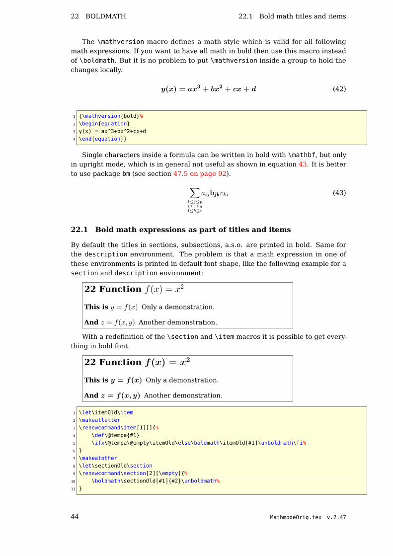
22 BOLDMATH 22.1 Bold math titles and items

The \mathversion macro defines a math style which is valid for all followingmath expressions. If you want to have all math in bold then use this macro insteadof \boldmath. But it is no problem to put \mathversion inside a group to hold thechanges locally.

y(x) = ax3 + bx2 + cx+ d (42)

1 \mathversionbold%2 \beginequation3 y(x) = ax^3+bx^2+cx+d4 \endequation

Single characters inside a formula can be written in bold with \mathbf, but onlyin upright mode, which is in general not useful as shown in equation 43. It is betterto use package bm (see section 47.5 on page 92).

∑


aijbjkcki (43)

22.1 Bold math expressions as part of titles and items

By default the titles in sections, subsections, a.s.o. are printed in bold. Same forthe description environment. The problem is that a math expression in one ofthese environments is printed in default font shape, like the following example for asection and description environment:

22 Function f(x) = x2

This is y = f(x) Only a demonstration.

And z = f(x, y) Another demonstration.

With a redefinition of the \section and \item macros it is possible to get every-thing in bold font.

22 Function f(x) = x2

This is y = f(x) Only a demonstration.

And z = f(x, y) Another demonstration.

1 \let\itemOld\item2 \makeatletter3 \renewcommand\item[1][]%4 \def\@tempa#15 \ifx\@tempa\@empty\itemOld\else\boldmath\itemOld[#1]\unboldmath\fi%6 7 \makeatother8 \let\sectionOld\section9 \renewcommand\section[2][\empty]%

10 \boldmath\sectionOld[#1]#2\unboldmath%11


24 OTHER MACROS

23 Multiplying numbers

When the dot is used as the decimal marker as in the United States, the preferredsign for the multiplication of numbers or values of quantities is a cross (\times × ),not a half-high and centered dot (\cdot · ).

When the comma is used as the decimal marker as in Europe, the preferred signfor the multiplication of numbers is the half-high dot. The multiplication of quantitysymbols (or numbers in parentheses or values of quantities in parentheses) may beindicated in one of the following ways: ab, a · b, a× b.

For more information see “Nist Guide to SI Units -More on Printing and UsingSymbols and Numbers in Scientific and Technical Documents”18 or the German DIN1304, Teil 1.

24 Other macros\everymath\everydisplay\underline

There are some other macros which are not mentioned in the foregoing text. Herecomes a not really complete list of these macros.

\everymath puts the argument before any inlined math expression, e.g., \everymath\displaysize.Using this macro doesn’t really make sense, when one is using footnotes be-cause the footnote number is printed as superscript in inline mathmode and an\everymath will be valid, too.

\everydisplay puts the argument before any displayed math expression, e.g.,\everydisplay\colorblue.

\underline underlines a math expression and has to be used inside the math mode.

F (x) =

ˆf(x) dx

18http://physics.nist.gov/Pubs/SP811/sec10.html


http://physics.nist.gov/Pubs/SP811/sec10.html

25 ALIGN ENVIRONMENTS

Part II

AMSmath package

In general the AMS packages are at least a collection of three different ones:

1. amsmath.sty

2. amssymb.sty

3. amsfonts.sty

In the following only the first one is described in detail.The AMSmath has the following options:

centertags (default) For a split equation, place equation numbers verticallycentered on the total height of the equation.

tbtags ‘Top-or-bottom tags’ For a split equation, place equation numberslevel with the last (resp. first) line, if numbers are on the right (resp.left).

sumlimits (default) Place the subscripts and superscripts of summation sym-bols above and below, in displayed equations. This option alsoaffects other symbols of the same type –

∏,∐

,⊗

,⊕

, and so forth –but excluding integrals (see below).

nosumlimits Always place the subscripts and superscripts of summation-typesymbols to the side, even in displayed equations.

intlimits Like sumlimits, but for integral symbols.

nointlimits (default) Opposite of intlimits.

namelimits (default) Like sumlimits, but for certain ‘operator names’ such asdet, inf, lim, max, min, that traditionally have subscripts placedunderneath when they occur in a displayed equation.

nonamelimits Opposite of namelimits.

To use one of these package options, put the option name in the optional argu-ment, e.g., \usepackage[intlimits]amsmath. The AMSmath also recognises thefollowing options which are normally selected (implicitly or explicitly) through thedocumentclass command, and thus need not be repeated in the option list of the\usepackageamsmath statement.

leqno Place equation numbers on the left.

reqno (default) Place equation numbers on the right.

fleqn Position equations at a fixed indent from the left margin rather than centeredin the text column. AMSmath defines the length \mathindent and uses itwhen the equations have only one tabbing character (&).

All math environments are displayed ones, so there is no special inline math.

25 align environments

There are four different align environments, described in the following subsections.Their behaviour is shown in table 15. The symbolic code for all align environments is:


25.1 The default align environment 25 ALIGN ENVIRONMENTS

1 \begin<name>2 <name> &= x & x &= x\\3 <name> &= x & x &= x4 \end<name>

Table 15: Comparison between the different align environments with the same code,where the first three can have an equation number

align = x x = x

align = x x = x

alignat = x x = x

alignat = x x = x

flalign = x x = x

flalign = x x = x

xalignat = x x = x

xalignat = x x = x

xxalignat = x x = x

xxalignat = x x = x

In difference to the eqnarray environment from standard LATEX (section 3.2),the “three” parts of one equation expr.-symbol-expr. are divided by only oneampersand in two parts. In general the ampersand should be before the symbolto get the right spacing, e.g., y &= x. Compare the following three equations, thesecond one has a wrong spacing.

y = x

y =x

y = x

1 y &= x

2 y =& x

3 y =& x

25.1 The default align environment

The eqnarray environment has a not so good spacing between the cells. Writing theequations no. 3 to 6 with the align environment gives:


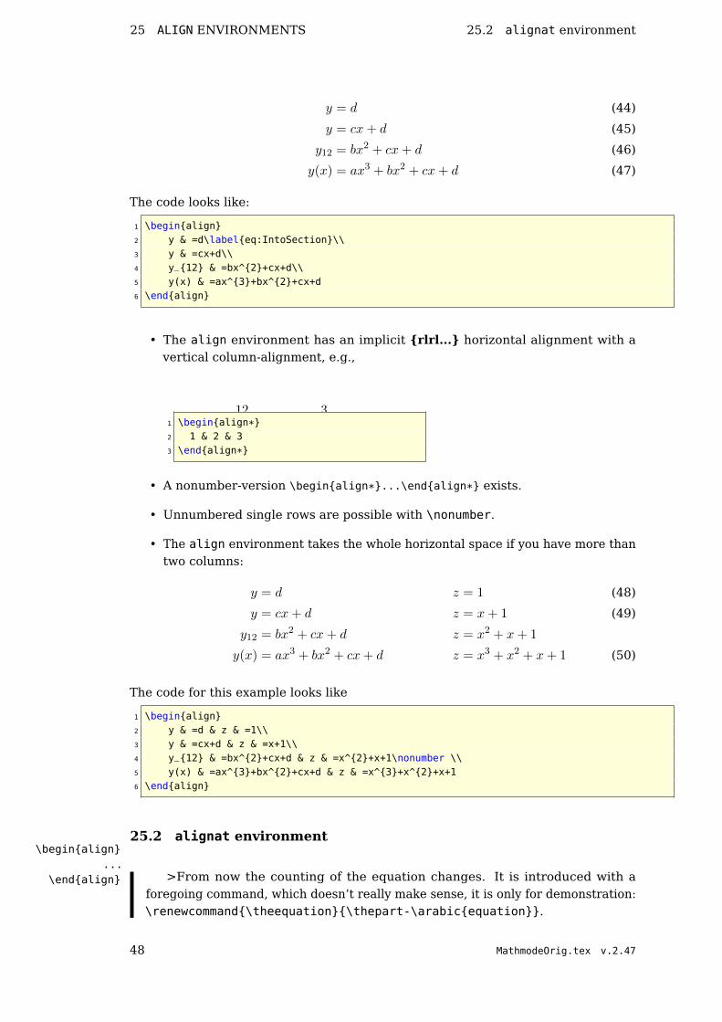
25 ALIGN ENVIRONMENTS 25.2 alignat environment

y = d (44)

y = cx+ d (45)

y12 = bx2 + cx+ d (46)

y(x) = ax3 + bx2 + cx+ d (47)

The code looks like:

1 \beginalign2 y & =d\labeleq:IntoSection\\3 y & =cx+d\\4 y_12 & =bx^2+cx+d\\5 y(x) & =ax^3+bx^2+cx+d6 \endalign

• The align environment has an implicit rlrl... horizontal alignment with avertical column-alignment, e.g.,

12 31 \beginalign*2 1 & 2 & 33 \endalign*

• A nonumber-version \beginalign*...\endalign* exists.

• Unnumbered single rows are possible with \nonumber.

• The align environment takes the whole horizontal space if you have more thantwo columns:

y = d z = 1 (48)

y = cx+ d z = x+ 1 (49)

y12 = bx2 + cx+ d z = x2 + x+ 1

y(x) = ax3 + bx2 + cx+ d z = x3 + x2 + x+ 1 (50)

The code for this example looks like

1 \beginalign2 y & =d & z & =1\\3 y & =cx+d & z & =x+1\\4 y_12 & =bx^2+cx+d & z & =x^2+x+1\nonumber \\5 y(x) & =ax^3+bx^2+cx+d & z & =x^3+x^2+x+16 \endalign

25.2 alignat environment\beginalign

...\endalign >From now the counting of the equation changes. It is introduced with a

foregoing command, which doesn’t really make sense, it is only for demonstration:\renewcommand\theequation\thepart-\arabicequation.


25.3 flalign environment 25 ALIGN ENVIRONMENTS

This means “align at several places” and is something like more than two alignenvironment side by side. Parameter is the number of the align environments, whichis not important for the user. The above last align example looks like:

y = d z = 1 (II-51)

y = cx+ d z = x+ 1 (II-52)

y12 = bx2 + cx+ d z = x2 + x+ 1

y(x) = ax3 + bx2 + cx+ d z = x3 + x2 + x+ 1 (II-53)

The parameter was 2 and it is 3 for the following example:

i11 = 0.25 i12 = i21 i13 = i23

i21 =1

3i11 i22 = 0.5i12 i23 = i31 (II-54)

i31 = 0.33i22 i32 = 0.15i32 i33 = i11 (II-55)

For this example the code is:

1 \beginalignat32 i_11 & =0.25 & i_12 & =i_21 & i_13 & =i_23\nonumber\\3 i_21 & =\frac13i_11 & i_22 & =0.5i_12& i_23 & =i_31\\4 i_31 & =0.33i_22\quad & i_32 & =0.15i_32\quad & i_33 & =i_115 \endalignat

With the alignat environment one can easily align equations vertically at morethan one marker:

abc = xxx = xxxxxxxxxxxx = aaaaaaaaa (II-56)

ab = yyyyyyyyyyyyyyy = yyyy = ab (II-57)

1 \beginalignat32 abc &= xxx &&= xxxxxxxxxxxx &&= aaaaaaaaa \\3 ab &= yyyyyyyyyyyyyyy &&= yyyy &&= ab4 \endalignat

• The alignat environment has an implicit rlrl...rlrl horizontal alignment witha vertical column alignment.

• A nonumber-version \beginalignat*...\endalignat* exists.

• Unnumbered single rows are possible with \nonumber.

25.3 flalign environment\beginflalign...\endflalign

This is the new replacement for the xalignat and xxalignat environments. It isnearly the same as the xalignat environment, only more “out spaced” and “leftaligned”.


25 ALIGN ENVIRONMENTS 25.3 flalign environment

i11 = 0.25

i21 =1

3i11 (II-58)

i31 = 0.33i22 (II-59)1 \beginflalign2 i_11 & =0.25\nonumber \\3 i_21 & =\frac13i_11\\4 i_31 & =0.33i_225 \endflalign

As seen, the equations are not really left aligned, when they have only oneampersand. In this case flalign has the same behaviour as the align environment.

When there are more than one tabbing characters (&), then the equations arereally left aligned. This is also an easy way to get an equation with only oneampersand left aligned, see equation II-63 below.

i11 = 0.25 i12 = i21 i13 = i23

i21 =1

3i11 i22 = 0.5i12 i23 = i31 (II-60)

i31 = 0.33i22 i32 = 0.15i32 i33 = i11 (II-61)


1 \beginflalign2 i_11 & =0.25 & i_12 & =i_21 & i_13 & =i_23\nonumber\\3 i_21 & =\frac13i_11 & i_22 & =0.5i_12& i_23 & =i_31\\4 i_31 & =0.33i_22\quad & i_32 & =0.15i_32\quad & i_33 & =i_115 \endflalign

This environment can be used to mix centered and left aligned equations withoutusing the document wide valid option fleqn.

f(x) =

ˆ1

x2dx (II-62)

f(x) =

ˆ1

x2dx (II-63)

Equation II-63 is left aligned in fact of the second tabbing character &.

1 \beginalign\labeleq:centered2 f(x) & = \int\frac1x^2\,\mathrmdx3 \endalign4

5 \beginflalign\labeleq:leftaligned6 f(x) & = \int\frac1x^2\,\mathrmdx &7 \endflalign

Another case is placing text left aligned, whereas the formulas should be rightaligned.

12(x− 1) + 20(y − 3) + 14(z − 2) = 0

same as 6x+ 10y + 7z = 0


25.4 xalignat environment 25 ALIGN ENVIRONMENTS

1 \beginflalign*2 && 12(x-1)+20(y-3)+14(z-2) &= 0\\3 \textsame as && 6x+10y+7z &= 04 \endflalign*

25.4 xalignat environment\beginxalignat...\endxalignat

This is an obsolete macro but still supported by the AMSmath package. Same asalignat environment, only a little more “out spaced”.

i11 = 0.25 i12 = i21 i13 = i23

i21 =1

3i11 i22 = 0.5i12 i23 = i31 (II-64)

i31 = 0.33i22 i32 = 0.15i32 i33 = i11 (II-65)

The same code looks like:

1 \beginxalignat32 i_11 & =0.25 & i_12 & =i_21 & i_13 & =i_23\nonumber\\3 i_21 & =\frac13i_11 & i_22 & =0.5i_12& i_23 & =i_31\\4 i_31 & =0.33i_22\quad & i_32 & =0.15i_32\quad & i_33 & =i_115 \endxalignat

25.5 xxalignat environment\beginxxalignat...\endxxalignat

Like xalignat an obsolete macro but still supported by the AMSmath package.Same as align environment, only extremely “out spaced”, therefore no equationnumber!

i11 = 0.25 i12 = i21 i13 = i23

i21 =1

3i11 i22 = 0.5i12 i23 = i31

i31 = 0.33i22 i32 = 0.15i32 i33 = i11

The same code looks like:

1 \beginxxalignat32 i_11 & =0.25 & i_12 & =i_21 & i_13 & =i_23\nonumber\\3 i_21 & =\frac13i_11 & i_22 & =0.5i_12& i_23 & =i_31\\4 i_31 & =0.33i_22 & i_32 & =0.15i_32 & i_33 & =i_115 \endxxalignat

25.6 aligned environment\beginaligned...\endaligned

In difference to the split environment (section 26.4 on page 57), the aligned envi-ronment allows more than one horizontal alignment but has also only one equationnumber:

2x+ 3 = 7 2x+ 3− 3 = 7− 3

2x = 42x

2=

4

2

x = 2

(II-66)


26 OTHER ENVIRONMENTS 25.7 Problems

1 \beginequation2 \beginaligned3 2x+3 &= 7 & 2x+3-3 &= 7-3 \\4 2x &= 4 & \frac2x2 &= \frac42\\5 x &= 26 \endaligned7 \endequation

The aligned environment is similar to the array environment, there exists nostarred version and it has only one equation number and has to be part of an-other math environment, which should be equation environment. The advantage ofaligned is the much better horizontal and vertical spacing.

25.7 Problems

When using one of the align environments, there should be no \\ at the end of thelast line, otherwise you’ll get another equation number for this “empty” line:

2x+ 3 = 7 (II-67)

(II-68)1 \beginalign2 2x+3 &= 7\\3 \endalign

2x+ 3 = 7 (II-69)1 \beginalign2 2x+3 &= 73 \endalign

26 Other environments

26.1 gather environment\begingather

...\endgather

This is like a multi line environment with no special horizontal alignment. All rowsare centered and can have an own equation number:

i11 = 0.25 (II-70)

i21 =1

3i11

i31 = 0.33i22 (II-71)

For this example the code looks like:

1 \begingather2 i_11 = 0.25\\3 i_21 = \frac13i_11\nonumber\\4 i_31 =0.33i_225 \endgather

• The gather environment has an implicit c horizontal alignment with novertical column alignment. It is just like an one column array/table.


26.2 gathered environment 26 OTHER ENVIRONMENTS

• A nonumber-version \begingather*...\endgather* exists. Look at sec-tion 26.4 on page 57 for an example.

26.2 gathered environment\begingathered[c]...\endgathered

The gathered environment is like the aligned or alignat environment. They useonly so much horizontal space as the widest line needs. In difference to the gatherenvironment it must be itself inside the math mode.

i11 = 0.25

i21 =1

3i11

i31 = 0.33i22

(II-72)

1 \beginalign2 \rule2cm1pt3 \begingathered4 \quad i_11=0.25\\5 \quad i_21=\frac13i_11\\6 \quad i_31=0.33i_227 \endgathered8 \rule2cm1pt9 \endalign

The optional argument can be used for setting the vertical alignment which is bydefault c (centered). It can also be t for top or b for bottom.

A = a

B = b

C = c

A = a

B = b

C = c

A = a

B = b

C = c (II-73)

1 \beginalign2 \rule1cm1pt3 \begingathered[t]4 \quad A=a\\5 \quad B=b\\6 \quad C=c7 \endgathered8 %9 \begingathered[c]

10 \quad A=a\\11 \quad B=b\\12 \quad C=c13 \endgathered14 %15 \begingathered[b]16 \quad A=a\\17 \quad B=b\\18 \quad C=c19 \endgathered20 \ \rule1cm1pt21 \endalign


26 OTHER ENVIRONMENTS 26.3 multline environment

When using a square bracket as first character inside the environment, theneverything is ignored by AMS until a following closing bracket, because AMS takesthis as an optional argument:

A = a

[B] B = b

[C] C = c

(II-74)

1 \beginalign2 \begingathered3 [A]\quad A=a\\4 [B]\quad B=b\\5 [C]\quad C=c6 \endgathered7 \endalign

The [A] is completely ignored, which can be avoided by using the optional argument[c] or at least an empty one directly after the \begingather. Another possibilityis using the package empheq, which fixes this behaviour by default.

[A] A = a

[B] B = b

[C] C = c

(II-75)

1 \beginalign2 \begingathered[]3 [A]\quad A=a\\4 [B]\quad B=b\\5 [C]\quad C=c6 \endgathered7 \endalign

26.3 multline environment\beginmultline

...\endmultline

This is also like a multi line19 environment with a special vertical alignment. Thefirst row is left aligned, the second and all following ones except the last one arecentered and the last line is right aligned. It is often used to write extremely longformulas:

1 \beginmultline2 A = \lim _n\rightarrow \infty \Delta x\left( a^2+\left( a^2+2a\Delta x3 +\left( \Delta x\right) ^2\right)\right.\\4 +\left( a^2+2\cdot 2a\Delta x+2^2\left( \Delta x\right) ^2\right)\\5 +\left( a^2+2\cdot 3a\Delta x+3^2\left( \Delta x\right) ^2\right)\\6 + \ldots\\7 \left.+\left( a^2+2\cdot (n-1)a\Delta x +(n-1)^2\left( \Delta x\right) ^2\right) \right)\\8 = \frac13\left( b^3-a^3\right)9 \endmultline

19It is no typo, the name of the environment is multline, no missing i here!


26.3 multline environment 26 OTHER ENVIRONMENTS

A = limn→∞

∆x(a2 +

(a2 + 2a∆x+ (∆x)2

)

+(a2 + 2 · 2a∆x+ 22 (∆x)2

)

+(a2 + 2 · 3a∆x+ 32 (∆x)2

)

+ . . .

+(a2 + 2 · (n− 1)a∆x+ (n− 1)2 (∆x)2

))

=1

3

(b3 − a3

)(II-76)

x

x

x

x

x

x (II-77)

Figure 1: multline Alignment demo (the fourth row is shifted to the right with\shoveright)

\multlinegap=

10.0pt (II-78)

\multlinegap=

0.0pt (II-79)

Figure 2: Demonstration of \multlinegap (default is 0pt)

• A nonumber-version \beginmultline*...\endmultline* exists.

• By default only the last line (for right equation numbers) or the first line (forleft equation numbers) gets a number, the others can’t.

• The alignment of a single line can be changed with the command \shoveright(figure 1)

• The first line and the last line have a small gap to the text border.20 See figure2, where the length of \multlinegap is set to 0pt for the right one.

26.3.1 Examples for multline

With the multline environment the equation 28 on page 27 looks like:

20When the first (numbers left) or last line (numbers right) has an equation number then\multlinegap is not used for these ones, only for the line without a number.


26 OTHER ENVIRONMENTS 26.3 multline environment

1

2∆(fijf

ij) = 2

∑

i<j


+ ∇kfij∇kf ij + f ijfk [2∇iRjk −∇kRij ])

(II-80)

which is again a bad typesetting because of the two unequal parentheses. Each onehas a size which is correct for the line but not for the whole formula. LATEX acceptsonly pairs of parentheses for one line and has an “empty” parentheses, the dot“\left.” or “\right.” to get only one of the “pair”. There are different solutions toget the right size of the parentheses. One of them is to use the \vphantom command,which reserves the vertical space without any horizontal one, like a vertical rulewithout any thickness. The sum symbol from the first line is the biggest one andresponsible for the height, so this one is the argument of \vphantom which has to beplaced anywhere.

1

2∆(fijf

ij) = 2

∑

i<j


+∇kfij∇kf ij + f ijfk [2∇iRjk −∇kRij ]

(II-81)

1 \beginmultline2 \frac12\Delta(f_ijfîj)=3 2\left(\sum_i<j\chi_ij(\sigma_i-4 \sigma_j)^2+fîj\nabla_j\nabla_i(\Delta f)+\right.\\5 \left.+\nabla_kf_ij\nabla^kfîj+6 fîjf^k\left[2\nabla_iR_jk-7 \nabla_kR_ij\right]\vphantom\sum_i<j\right)8 \endmultline

Instead of using the \vphantom command it is also possible to use fixed-width paren-theses, which is described in section 8 on page 24.

A math expression with a very long fraction like the following one, which runsout of the margin could be written as a multiplication to avoid the fraction line.

dG∞dn

=[1− e−pn] [Q (n)− pR (n) +R′ (n)] e−pn −

[−Q(n)e−pn

p + Q(0)p +R (n) e−pn −A

]pe−pn

(1− e−pn)2 = 0

(II-82)

1 \beginequation2 \frac\mathrmdG_\infty\mathrmdn=\frac\left[1-e^-pn\right]3 \left[Q\left(n\right)-pR\left(n\right)+R’\left(n\right)\right]e^-pn4 -\left[-\fracQ \left(n\right)e^-pnp+\fracQ\left(0\right)p+R5 \left(n\right)e^-pn - A\right] pe^-pn\left(1-e^-pn\right)^2 = 06 \endequation

With the multline environment it can then be split into two or more parts:


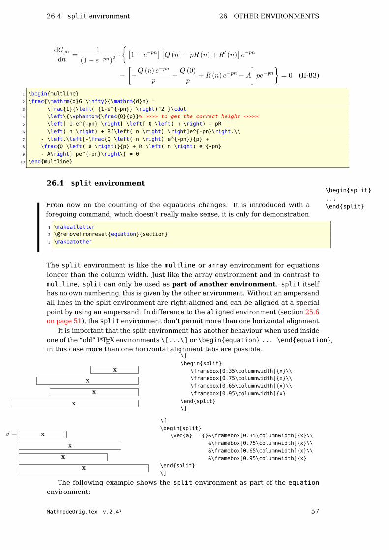
26.4 split environment 26 OTHER ENVIRONMENTS

dG∞dn

=1

(1− e−pn)2 ·[

1− e−pn] [Q (n)− pR (n) +R′ (n)

]e−pn

−[−Q (n) e−pn

p+Q (0)

p+R (n) e−pn −A

]pe−pn

= 0 (II-83)

1 \beginmultline2 \frac\mathrmdG_\infty\mathrmdn =3 \frac1\left( 1-e^-pn \right)^2 \cdot4 \left\\vphantom\fracQp% >>>> to get the correct height <<<<<5 \left[ 1-e^-pn \right] \left[ Q \left( n \right) - pR6 \left( n \right) + R’\left( n \right) \right]e^-pn\right.\\7 - \left.\left[-\fracQ \left( n \right) e^-pnp +8 \fracQ \left( 0 \right)p + R \left( n \right) e^-pn9 - A\right] pe^-pn\right\ = 0

10 \endmultline

26.4 split environment\beginsplit...\endsplitFrom now on the counting of the equations changes. It is introduced with a

foregoing command, which doesn’t really make sense, it is only for demonstration:

1 \makeatletter2 \@removefromresetequationsection3 \makeatother

The split environment is like the multline or array environment for equationslonger than the column width. Just like the array environment and in contrast tomultline, split can only be used as part of another environment. split itselfhas no own numbering, this is given by the other environment. Without an ampersandall lines in the split environment are right-aligned and can be aligned at a specialpoint by using an ampersand. In difference to the aligned environment (section 25.6on page 51), the split environment don’t permit more than one horizontal alignment.

It is important that the split environment has another behaviour when used insideone of the “old” LATEX environments \[...\] or \beginequation ... \endequation,in this case more than one horizontal alignment tabs are possible.

x

x

x

x

\[\beginsplit

\framebox[0.35\columnwidth]x\\\framebox[0.75\columnwidth]x\\\framebox[0.65\columnwidth]x\\\framebox[0.95\columnwidth]x

\endsplit\]

~a = x

x

x

x

\[\beginsplit

\veca = &\framebox[0.35\columnwidth]x\\&\framebox[0.75\columnwidth]x\\&\framebox[0.65\columnwidth]x\\&\framebox[0.95\columnwidth]x

\endsplit\]

The following example shows the split environment as part of the equationenvironment:


26 OTHER ENVIRONMENTS 26.4 split environment

A1 =

∣∣∣∣ˆ 1

0(f(x)− g(x)) dx

∣∣∣∣+

∣∣∣∣ˆ 2

1(g(x)− h(x)) dx

∣∣∣∣

=

∣∣∣∣ˆ 1

0(x2 − 3x) dx

∣∣∣∣+

∣∣∣∣ˆ 2

1(x2 − 5x+ 6) dx

∣∣∣∣

=

∣∣∣∣x3

3− 3

2x2

∣∣∣∣1

0

+

∣∣∣∣x3

3− 5

2x2 + 6x

∣∣∣∣2

1

=

∣∣∣∣1

3− 3

2

∣∣∣∣+

∣∣∣∣8

3− 20

2+ 12−

(1

3− 5

2+ 6

)∣∣∣∣

=

∣∣∣∣−7

6

∣∣∣∣+

∣∣∣∣14

3− 23

6

∣∣∣∣ =7

6+

5

6= 2 FE

(II-84)

1 \beginequation2 \beginsplit3 A_1 & = \left| \int _0^1(f(x)-g(x))\,\mathrmdx\right| +\left|4 \int _1^2(g(x)-h(x))\,\mathrmdx\right| \\5 & = \left| \int _0^1(x^2-3x)\,\mathrmdx\right| +\left|6 \int _1^2(x^2-5x+6)\,\mathrmdx\right| \\7 & = \left| \fracx^33-\frac32x^2\right| _0^1+8 \left| \fracx^33-9 \frac52x^2+6x\right| _1^2\\

10 & = \left| \frac13-\frac32\right| +\left|11 \frac83-\frac202+12-12 \left( \frac13-\frac52+6\right) \right| \\13 & = \left| -\frac76\right| +\left| \frac143-\frac23614 \right| =\frac76+\frac56=2\, \textrmFE15 \endsplit16 \endequation

The same using the array environment with rl-alignment instead of splitgives same horizontal alignment, but another vertical spacing21 and the symbols areonly in scriptsize and not textsize:22

A1 =∣∣∣´ 1

0 (f(x)− g(x)) dx∣∣∣+∣∣∣´ 2

1 (g(x)− h(x)) dx∣∣∣

=∣∣∣´ 1

0 (x2 − 3x) dx∣∣∣+∣∣∣´ 2

1 (x2 − 5x+ 6) dx∣∣∣

=∣∣∣x33 − 3

2x2∣∣∣1

0+∣∣∣x33 − 5

2x2 + 6x

∣∣∣2

1=∣∣1

3 − 32

∣∣+∣∣8

3 − 202 + 12−

(13 − 5

2 + 6)∣∣

=∣∣−7

6

∣∣+∣∣14

3 − 236

∣∣ = 76 + 5

6 = 2 FE

(II-85)

Compare the following two examples for typesetting the minus sign. In the firstcase it is typeset similiar to the plus character, and in the second example it is typesetwithout the additional space for a binary math atom.

21Can be changed with \renewcommand\arraystretch1.522See section 12 on page 36


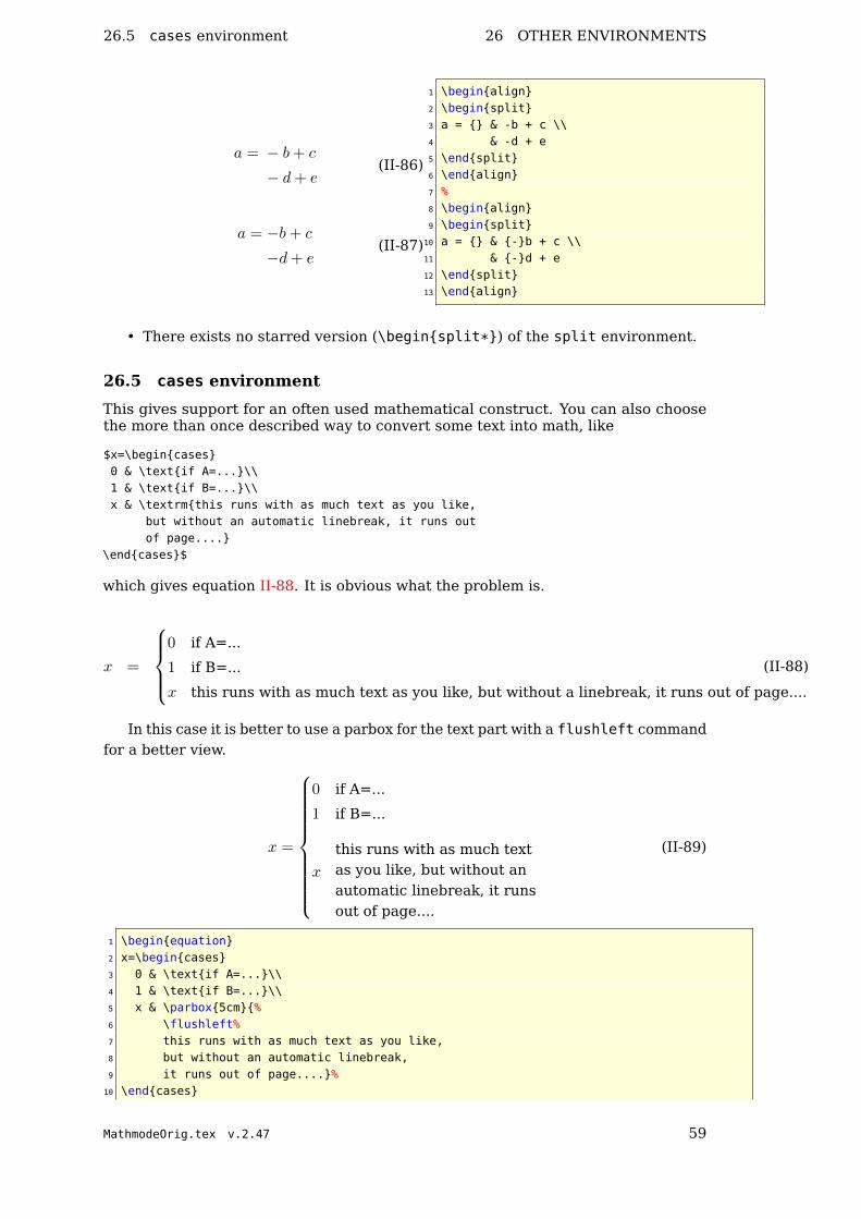
26.5 cases environment 26 OTHER ENVIRONMENTS

a = − b+ c

− d+ e(II-86)

a = −b+ c

−d+ e(II-87)

1 \beginalign2 \beginsplit3 a = & -b + c \\4 & -d + e5 \endsplit6 \endalign7 %8 \beginalign9 \beginsplit10 a = & -b + c \\11 & -d + e12 \endsplit13 \endalign

• There exists no starred version (\beginsplit*) of the split environment.

26.5 cases environment

This gives support for an often used mathematical construct. You can also choosethe more than once described way to convert some text into math, like

$x=\begincases0 & \textif A=...\\1 & \textif B=...\\x & \textrmthis runs with as much text as you like,

but without an automatic linebreak, it runs outof page....

\endcases$

which gives equation II-88. It is obvious what the problem is.

x =

0 if A=...

1 if B=...

x this runs with as much text as you like, but without a linebreak, it runs out of page....

(II-88)

In this case it is better to use a parbox for the text part with a flushleft commandfor a better view.

x =

0 if A=...

1 if B=...

x

this runs with as much textas you like, but without anautomatic linebreak, it runsout of page....

(II-89)

1 \beginequation2 x=\begincases3 0 & \textif A=...\\4 1 & \textif B=...\\5 x & \parbox5cm%6 \flushleft%7 this runs with as much text as you like,8 but without an automatic linebreak,9 it runs out of page....%

10 \endcases


28 DOTS 26.6 Matrix environments

11 \endequation

From now on the counting of the equations changes. It is introduced with aforegoing command, which doesn’t really make sense, it is only for demonstration:

1 \renewcommand\theequation\arabicequation

26.6 Matrix environments

\Vmatrix

∥∥∥∥a bc d

∥∥∥∥ \Bmatrix

a bc d

\matrix

a bc d

\vmatrix

∣∣∣∣a bc d

∣∣∣∣ \bmatrix

[a bc d

]\pmatrix

(a bc d

)

\smallmatrix a bc d

Table 16: Matrix environments

All matrix environments can be nested and an element may also contain anyother math environment, so that very complex structures are possible. By default allcells have a centered alignment, which is often not the best when having differentdecimal numbers or plus/minus values. Changing the alignment to right (not for thesmallmatrix) is possible withmatrix

vmatrixVmatrixbmatrixBmatrixpmatrix

smallmatrix

1 \makeatletter2 \def\env@matrix\hskip -\arraycolsep3 \let\@ifnextchar\new@ifnextchar4 \array*\c@MaxMatrixCols r5 \makeatother

The special matrix environment smallmatrix, which decreases horizontal andvertical space is typeset in scriptstyle. The smallmatrix environment makes somesense in the inline mode to decrease the line height. For dots over several columnslook for \hdotsfor in the following section.

27 Vertical whitespace

See section 11.5 on page 33 for the lengths which control the vertical whitespace.There is no difference to AMSmath.

28 Dots

In addition to section 13 on page 37 AMSmath has two more commands for dots:\dddot...23 and \ddddot...

$\dddoty$:...y

$\ddddoty$:....y

Another interesting dot command is \hdotsfor with the syntax:

1 \hdotsfor[<spacing factor>]<number of columns>

23already mentioned in section 14


29 FRACTION COMMANDS

With the spacing factor the width of the dots can be stretched or shrinked. Thenumber of columns allows a continuing dotted line over more columns. Equation 90shows the definition of a tridiagonal matrix.

A =

a11 a12 0 . . . . . . . . . 0

a21 a22 a23 0 . . . . . . 0

0 a32 a33 a34 0 . . . 0...

......

......

......

. . . . . . . . . . . . . . . . . . . . . . . . . . . . . . . . . . . . . . . . . . . . . . . . . . . . ....

......

......

......

0 . . . 0 an−2,n−3 an−2,n−2 an−2,n−1 0

0 . . . . . . 0 qn−1,n−2 an−1,n−1 an−1,n

0 . . . . . . . . . 0 an,n−1 ann

(90)

1 \beginequation2 \underlineA=\left[\beginarrayccccccc3 a_11 & a_12 & 0 & \ldots & \ldots & \ldots & 0\\4 a_21 & a_22 & a_23 & 0 & \ldots & \ldots & 0\\5 0 & a_32 & a_33 & a_34 & 0 & \ldots & 0\\6 \vdots & \vdots & \vdots & \vdots & \vdots & \vdots & \vdots\\7 \hdotsfor7\cr\vdots & \vdots & \vdots & \vdots & \vdots & \vdots & \vdots\\8 0 & \ldots & 0 & a_n-2,n-3 & a_n-2,n-2 & a_n-2,n-1 & 0\\9 0 & \ldots & \ldots & 0 & q_n-1,n-2 & a_n-1,n-1 & a_n-1,n\\

10 0 & \ldots & \ldots & \ldots & 0 & a_n,n-1 & a_nn11 \endarray\right]12 \endequation

29 fraction commands

29.1 Standard

Additional to the font size problem described in subsection 2.2 on page 10 AMSmathsupports some more commands for fractions. The \frac command described in [7],does no more exist in AMSmath.

• The global fraction definition has five parameters

1 \genfrac<left delim><right delim><thickness><mathstyle><nominator><denominator>

where thickness can have any length with a valid unit likegenfrac1ptx^2+x+13x-2→ x2+x+1

3x−2

• \cfrac (continued fraction) which is by default set in the display mathstyle anduseful for fractions like

1

√2 +

1

√3 +

1

√4 +

1

. . .

(91)


30 ROOTS 29.2 Binoms

which looks with the default \frac command like

1√2 + 1√

3+ 1√4+ 1

...

(92)

where the mathstyle decreases for every new level in the fraction. The \cfraccommand can be called with an optional parameter which defines the placingof the nominator, which can be [l]eft, [r]ight or [c]enter (the default - seeequation 91):

1

√2 +

1

√3 +

1

√4 +

1

. . .

1

√2 +

1

√3 +

1

√4 +

1

. . .

• \dfrac which takes by default the displaystyle, so that fractions in inline mode1

2have the same size than in display mode.

• \tfrac (vice versa to \dfrac) which takes by default the scriptstyle, so thatfractions in display mode have the same size than in inline mode.

23 \tfrac23

2

3\frac23

29.2 Binoms\binom

\dbinom\tbinom

They are like fractions without a rule and its syntax is different to the \choosecommand from standard LATEX (see section 2.2 on page 10). AMSmath providesthree different commands for binoms just like the ones for fractions.

Command Inlinemath Displaymath

\binommn(mn

) (m

n

)

\dbinommn

(m

n

) (m

n

)

\tbinommn(mn

) (mn

)

Table 17: binom commands

30 Roots

The typesetting for roots is sometimes not the best. Some solutions for bettertypesetting are described in section 7 on page 23 for standard LATEX. AMSmath has\leftroot

\uproot some more commands for the n-th root:

1 \sqrt[\leftroot<number>\uproot<number><root>]< ... >


30.1 Roots with \smash command 32 \MOD COMMAND

<number> indicates a value for the points24 of which the root can be adjusted to theleft and/or to the top, e.g., kn

√a ($\sqrt[k_n]a$) has a too deep exponent, whereas

kn√a $\sqrt[\uproot2k_n]a$ looks nicer.

30.1 Roots with \smash command\smash

The default for a root with λki as root argument looks like√λki , which may be not the

best typesetting. It is possible to reduce the lowest point of the root to the baseline

with the \smash command:√λki

with \smash−−−−−−−→√λki

The syntax of the \smash command25 renewed by the AMSmath package is

1 \smash[<position>]<argument>

The optional argument for the position can be:

t keeps the bottom and annihilates the top

b keeps the top and annihilates the bottom

tb annihilates top and bottom (the default)

31 Accents

With the macro \mathaccent it is easy to define new accent types, for example

1 \def\dotcup$\mathaccent\cdot\cup$

·∪Overwriting of two symbols is also possible:

xyyxIn this case the second symbol has to be shifted to the left for a length of 5mu

(mu: math unit).

1 \def\curvearrowleftright%2 \ensuremath%3 \mathaccent\curvearrowright\mkern-5mu\curvearrowleft%4 %5

For other possibilities to define new accents see section 47.1 on page 90.

32 \mod command

In standard LATEX the modulo command is not an operator, though it is often used informulas. AMSmath provides two (three) different commands for modulo, which arelisted in tabular 18 on the following page.

• They all insert some useful space before and behind the mod-operator.


33 EQUATION NUMBERING

a\modnˆ2=b → a mod n2 = ba\pmodnˆ2=b → a (mod n2) = b

a\podnˆ2=b → a (n2) = b

Table 18: The modulo commands and their meaning

33 Equation numbering

See section 3.3 on page 14 for equation numbering. It is mostly the same, only one \numberwithin

command is new to AMSmath. If you want a numbering like “44” then write eitherin the preamble or like this example anywhere in your doc:

1 \numberwithinequationsection

From now on the numbering looks like equation 44 on page 48. For thebook-class you can get the same for chapters.

If you want to get rid of the parentheses then write in the preamble:

1 \makeatletter2 \def\tagform@#1\maketag@@@\ignorespaces#1\unskip\@@italiccorr3 \makeatother

Now the following four subequation numbers have no parentheses.

33.1 Subequations

Amsmath supports this with the environment subequation. For example:

y = d 33.93a

y = cx+ d 33.93b

y = bx2 + cx+ d 33.93c

y = ax3 + bx2 + cx+ d 33.93d

1 \beginsubequations2 \beginalign3 y & = d\\4 y & = cx+d\\5 y & = bx^2+cx+d\\6 y & = ax^3+bx^2+cx+d7 \endalign8 \endsubequations

Inside of subequations only complete other environments (\begin... ...\end...) are possible.

1 \renewcommand\theequation%2 \theparentequation-\arabicequation%3

24In PostScript units (bp – Big Points).25In latex.ltx \smash is defined without an optional argument.


34 LABELS AND TAGS

y = d (33.94-1)

y = cx+ d (33.94-2)

y = bx2 + cx+ d (33.94-3)

y = ax3 + bx2 + cx+ d (33.94-4)

A ref to a subequation is possible like the one to equation 33.94-2. The environ-ment chooses the same counter “equation” but saves the old value into “parentequation”.

It is also possible to place two equations side by side with counting as subfigures:

y = f(x) (33.95a) y = f(z) (33.95b)

In this case, the AMSmath internal subfigure counter cannot be used and an owncounter has to be defined:

1 \newcountermySubCounter2 \newcommand\twocoleqn[2]3 \setcountermySubCounter0%4 \let\OldTheEquation\theequation%5 \renewcommand\theequation\OldTheEquation\alphmySubCounter%6 \noindent%7 \beginminipage.49\textwidth8 \beginequation\refstepcountermySubCounter9 #1

10 \endequation11 \endminipage\hfill%12 \addtocounterequation-1%13 \beginminipage.49\textwidth14 \beginequation\refstepcountermySubCounter15 #216 \endequation17 \endminipage%18 \let\theequation\OldTheEquation19 20 [ ... ]21 \twocoleqny=f(x)y=f(z)

34 Labels and tags

For the \label command see section 3.4 on page 16, it is just the same behaviour. \tag

AMSmath allows to define own single “equation numbers” with the \tag command.

f(x) = a (linear)

g(x) = dx2 + cx+ b (quadratic)

h(x) = sinx trigonometric

1 \beginalign2 f(x) & =a\taglinear\labeleq:linear\\3 g(x) & =\,\mathrmdx^2+cx+b\tagquadratic\labeleq:quadratic\\4 h(x) & =\sin x\tag*trigonometric5 \endalign

• The \tag command is also possible for unnumbered equations, LATEX changesthe behaviour when a tag is detected.


35 LIMITS

• There exists a starred version \tag*..., which supresses any annotationslike parentheses for equation numbers.

• There exist two package options for tags, ctagsplit and righttag (look at thebeginning of this part on page 46).

35 Limits

By default the sum/prod has the limits above/below and the integral at the side.To get the same behaviour for all symbols which can have limits load the packageAMSmath in the preamble as

1 \usepackage[sumlimits,intlimits]amsmath

There exist also options for the vice versa (see page 46). See also Section 41 forthe additional commands \underset and \overset.

35.1 Multiple limits

For general information about limits read section 2.1 on page 9. Standard LATEXprovides the \atop command for multiple limits (section 6.1 on page 22). AMSmathhas an additional command for that, which can have several lines with the following\substack

syntax:\beginSb...

\endSb\beginSp

...\endSp

1 \substack...\\...\\...

The environments described in [7]

1 \beginSb ... \endSb2 \beginSp ... \endSp

are obsolete and no more part of AMSmath.The example equation 21 on page 22 with the \substack command looks like:

∑

1≤i≤p1≤j≤q1≤k≤r

aijbjkcki (35.1)

Insert these limits in the following way:

1 \beginequation2 \sum_%3 \substack1\le i\le p\\4 1\le j\le q\\5 1\le k\le r6 %7 a_ijb_jkc_ki8 \endequation

35.2 Problems

There are still some problems with limits and the following math expression. Forexample:

X =∑

1≤i≤j≤nXij


35.2 Problems 35 LIMITS

1 \[2 X = \sum_1\le i\le j\le nX_ij3 \]

does not look nice because of the long limit. Using a \makebox also does not reallysolve the problem, because \makebox is in TEX horizontal mode and knows nothingabout the appropriate math font size, because limits have a smaller font size. It isbetter to define a \mathclap macro, similiar to the two macros \llap and \rlap anduses the also new defined \mathclap macro:

1 \def\mathllap\mathpalette\mathllapinternal2 \def\mathllapinternal#1#2%3 \llap$\mathsurround=0pt#1#2$% $4 5 \def\clap#1\hbox to 0pt\hss#1\hss6 \def\mathclap\mathpalette\mathclapinternal7 \def\mathclapinternal#1#2%8 \clap$\mathsurround=0pt#1#2$%9

10 \def\mathrlap\mathpalette\mathrlapinternal11 \def\mathrlapinternal#1#2%12 \rlap$\mathsurround=0pt#1#2$% $13

Now we can write limits which have a boxwidth of 0pt and the right font size andthe following math expression appears just behind the symbol:

X =∑

1≤i≤j≤nXij

1 \[2 X = \sum_\mathclap1\le i\le j\le nX_ij3 \]

Another problem occurs when having operators with stacked limits in braces:

∑

i,ji>j

. . .

(35.2)

This case is not easy to handle when some other math expressions are around thebraces which should be on the same baseline. However, the following may help insome cases to get better looking braces.

foo

[∑

i,ji>j

. . .]bar (35.3)

1 \beginalign2 foo \left[\beginarray@c@3 \displaystyle\sum_\substacki,j\\i>j \dots4 \endarray\right] bar5 \endalign


36 OPERATOR NAMES 35.3 \sideset

35.3 \sideset

This is a command for a very special purpose, to combine over/under limits withsuperscript/subscripts for the sum-symbol. For example: it is not possible to place\sideset

the prime for the equation 35.4 near to the sum symbol, because it becomes an upperlimit when writing without an preceeding .

∑

n<kn odd

′nEn (35.4)

The command \sideset has the syntax

1 \sideset<before><behind>

It can place characters on all four corners of the sum-symbol:

TUpperLeft

LowerLeft

∑UpperRight

LowerRightB

1 \[2 \sideset_LowerLeft^UpperLeft_LowerRight^UpperRight\sum_B^T3 \]

Now it is possible to write the equation 35.4 in a proper way with the command\sideset’ before the sum symbol:

∑′

n<kn odd

nEn (35.5)

36 Operator names\operatorname

By default variables are written in italic and operator names in upright mode, likey = sin(x).26 This happens only for the known operator names, but creating a newone is very easy with:

1 \newcommand\mysin\operatornamemysin

Now \mysin is also written in upright mode y = mysin(x) and with some additionalspace before and behind.

It is obvious, that only those names can be defined as new operator names whichare not commands in another way. Instead of using the new definition as an operator,it is also possible to use the text mode. But it is better to have all operators of thesame type, so that changing the style will have an effect for all operators.\operatornamewithlimits

The new defined operator names cannot have limits, only superscript/subscript ispossible. amsopn.sty has an additional command \operatornamewithlimits, whichsupports over/under limits like the one from \int or \sum.\mathop

It is also possible to use the macro \mathop to declare anything as operator, like

1B

26See section 16 on page 40, where all the standard LATEX known operator names are listed. PackageAMSmath has some more (see documentation).


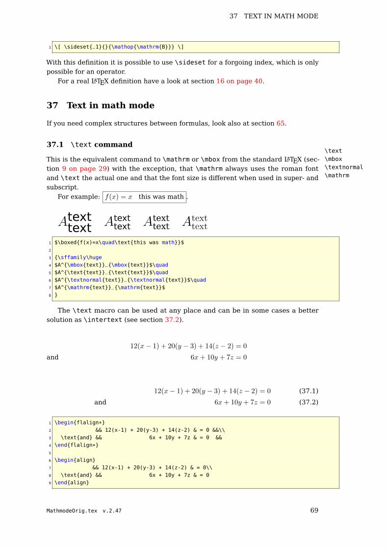
37 TEXT IN MATH MODE

1 \[ \sideset_1\mathop\mathrmB \]

With this definition it is possible to use \sideset for a forgoing index, which is onlypossible for an operator.

For a real LATEX definition have a look at section 16 on page 40.

37 Text in math mode

If you need complex structures between formulas, look also at section 65.

37.1 \text command\text\mbox\textnormal\mathrm

This is the equivalent command to \mathrm or \mbox from the standard LATEX (sec-tion 9 on page 29) with the exception, that \mathrm always uses the roman fontand \text the actual one and that the font size is different when used in super- andsubscript.

For example: f(x) = x this was math .

Atexttext Atexttext Atext

text Atexttext

1 $\boxedf(x)=x\quad\textthis was math$2

3 \sffamily\huge4 $A^\mboxtext_\mboxtext$\quad5 $A^\texttext_\texttext$\quad6 $A^\textnormaltext_\textnormaltext$\quad7 $A^\mathrmtext_\mathrmtext$8

The \text macro can be used at any place and can be in some cases a bettersolution as \intertext (see section 37.2).

12(x− 1) + 20(y − 3) + 14(z − 2) = 0

and 6x+ 10y + 7z = 0

12(x− 1) + 20(y − 3) + 14(z − 2) = 0 (37.1)

and 6x+ 10y + 7z = 0 (37.2)

1 \beginflalign*2 && 12(x-1) + 20(y-3) + 14(z-2) & = 0 &&\\3 \textand && 6x + 10y + 7z & = 0 &&4 \endflalign*5

6 \beginalign7 && 12(x-1) + 20(y-3) + 14(z-2) & = 0\\8 \textand && 6x + 10y + 7z & = 09 \endalign


38 EXTENSIBLE ARROWS 37.2 \intertext command

37.2 \intertext command

This is useful when you want to place some text between two parts of math stuffwithout leaving the math mode, like the name “intertext” says. For example we writethe equation II-84 on page 58 with an additional command after the second line.

A1 =

∣∣∣∣ˆ 1

0(f(x)− g(x)) dx

∣∣∣∣+

∣∣∣∣ˆ 2

1(g(x)− h(x)) dx

∣∣∣∣

=

∣∣∣∣ˆ 1

0(x2 − 3x) dx

∣∣∣∣+

∣∣∣∣ˆ 2

1(x2 − 5x+ 6) dx

∣∣∣∣

Now the limits of the integrals are used

=

∣∣∣∣x3

3− 3

2x2

∣∣∣∣1

0

+

∣∣∣∣x3

3− 5

2x2 + 6x

∣∣∣∣2

1

=

∣∣∣∣1

3− 3

2

∣∣∣∣+

∣∣∣∣8

3− 20

2+ 12−

(1

3− 5

2+ 6

)∣∣∣∣

=

∣∣∣∣−7

6

∣∣∣∣+

∣∣∣∣14

3− 23

6

∣∣∣∣ =7

6+

5

6= 2 FE


1 \beginequation2 \beginsplit3 A_1 & = \left| \int _0^1(f(x)-g(x))\,\mathrmdx\right| +\left| \int _1^2(g(x)-h(x))

\,\mathrmdx\right| \\4 & = \left| \int _0^1(x^2-3x)\,\mathrmdx\right| +\left| \int _1^2(x^2-5x+6)

\,\mathrmdx\right| \\5 \intertextNow the limits of the integrals are used6 & = \left| \fracx^33-\frac32x^2\right| _0^1+\left| \fracx^33-7 \frac52x^2+6x\right| _1^2\\8 & = \left| \frac13-\frac32\right| +\left| \frac83-\frac202+12-9 \left( \frac13-\frac52+6\right) \right| \\

10 & = \left| -\frac76\right| +\left| \frac143-\frac236\right| =\frac76+11 \frac56=2\, \textrmFE12 \endsplit13 \endequation

Writing very long text is possible by using a parbox, see section 9 on page 29 foran example with \textrm, which behaves in the same way as \text.

38 Extensible arrows\xrightarrow\xleftarrow

\xmapstoTo write something like

above the arrow−−−−−−−−−−→below

you can use the following macro

$\xrightarrow[\textbelow]\textabove the arrow$

and the same with \xleftarrow. You can define your own extensible arrow macros ifyou need other than these two predefined ones. To get a doublelined extensible arrowlike $\Longleftrightarrow$ (⇐⇒) but with the same behaviour as an extensibleone, write in the preamble


38 EXTENSIBLE ARROWS

1 \newcommand\xLongLeftRightArrow[2][]%2 \ext@arrow 0055\LongLeftRightArrowfill@#1#23 \def\LongLeftRightArrowfill@%4 \arrowfill@\Leftarrow\Relbar\Rightarrow5 \newcommand\xlongleftrightarrow[2][]%6 \ext@arrow 0055\longleftrightarrowfill@#1#27 \def\longleftrightarrowfill@%8 \arrowfill@\leftarrow\relbar\rightarrow

The three parts \Leftarrow\Relbar\Rightarrow define left|middle|right of thearrow, where the middle part would be stretched in a way that the arrow is at least aslong as the text above and/or below it. This macro has one optional and one standardparameter. The optional one is written below and the standard one above this arrow.Now we can write

$\xLongLeftRightArrow[\textbelow]\textabove the arrow$$\xlongleftrightarrow[\textbelow]\textabove the arrow$

to getabove the arrow⇐========⇒

belowor

above the arrow←−−−−−−−−→below

. The “number” 0055 after \ext@arrow defines

the position relative to the extended arrow and is not a number but four parametersfor additional space in the math unit mu.

1 \def\mapstofill@%2 \arrowfill@\mapstochar\relbar\relbar\rightarrow3 \newcommand*\xmapsto[2][]%4 \ext@arrow <four digits>\mapstofill@#1#2

$\ext@arrow 0000$over7−−−−→

under


under


under


under


under

$\ext@arrow 0099$over7−−−−−→

under

$\ext@arrow 9999$over7−−−−−→

under• 1st digit: space left

• 2nd digit: space right


40 GREEK LETTERS

• 3rd digit: space left and right

• 4th digit: space relativ to the tip of the “arrow”

The two macros \xrightarrow and \xleftarrow are defined as:

1 \newcommand\xrightarrow[2][]\ext@arrow 0359\rightarrowfill@#1#22 \newcommand\xleftarrow[2][]\ext@arrow 3095\leftarrowfill@#1#2

39 Frames\boxed

AMSmath knows the macro \boxed which can be used for inline a b+ c and dis-played math expressions:

f(x) =

ˆ ∞1

1

x2dx = 1 (39.1)

1 \beginalign2 \boxedf(x)=\int_1^\infty\frac1x^2\,\mathrmdx=13 \endalign

For coloured boxes use package empheq. For an example see section 47.11 onpage 96.

40 Greek letters\pmb

\boldsymbol The AMSmath package simulates a bold font for the greek letters by writing a greekcharacter twice with a small kerning. This is done with the macro \pmb<letter>.The \mathbf<character> doesn’t work with lower greek character. However,using the \boldsymbol macro from AMSmath is the better way when the font has abold symbol.

Uppercase greek letters are by default in upright mode. AMSmath supports alsosuch letters in italic mode with a preceeding var e.g., \varGamma

letter \pmbletter \boldsymbolletter letter italicα ααα α Γ Γ

β βββ β ∆ ∆

γ γγγ γ Θ Θ

δ δδδ δ Λ Λ

ε εεε ε Ξ Ξ

ε εεε ε Π Π

ζ ζζζ ζ Σ Σ

η ηηη η Υ Υ

θ θθθ θ Φ Φ

ϑ ϑϑϑ ϑ Ψ Ψ

ι ιιι ι Ω Ω

. . . . . . . . .


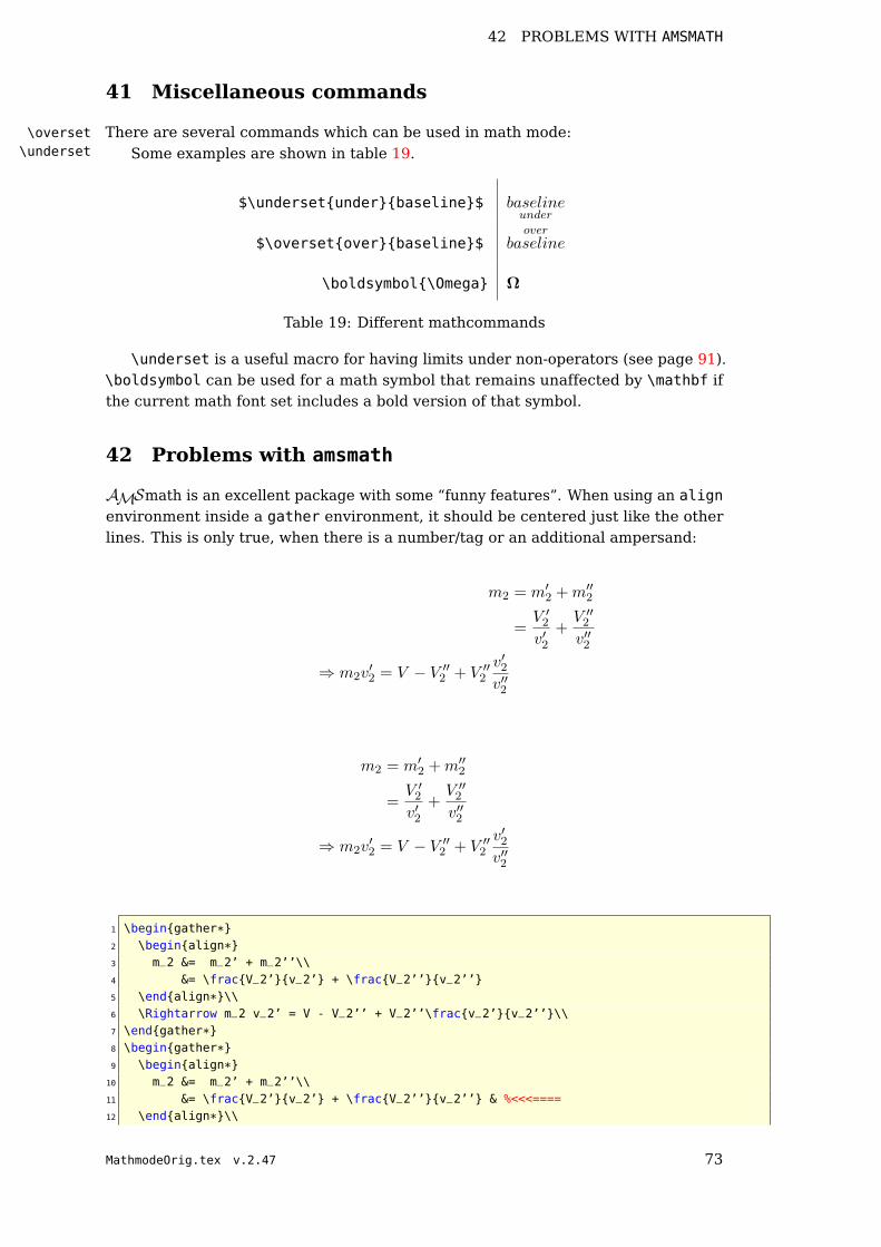
42 PROBLEMS WITH AMSMATH

41 Miscellaneous commands

There are several commands which can be used in math mode:\overset\underset Some examples are shown in table 19.

$\undersetunderbaseline$ baselineunder

$\oversetoverbaseline$over

baseline

\boldsymbol\Omega Ω

Table 19: Different mathcommands

\underset is a useful macro for having limits under non-operators (see page 91).\boldsymbol can be used for a math symbol that remains unaffected by \mathbf ifthe current math font set includes a bold version of that symbol.

42 Problems with amsmath

AMSmath is an excellent package with some “funny features”. When using an alignenvironment inside a gather environment, it should be centered just like the otherlines. This is only true, when there is a number/tag or an additional ampersand:

m2 = m′2 +m′′2

=V ′2v′2

+V ′′2v′′2

⇒ m2v′2 = V − V ′′2 + V ′′2

v′2v′′2

m2 = m′2 +m′′2

=V ′2v′2

+V ′′2v′′2

⇒ m2v′2 = V − V ′′2 + V ′′2

v′2v′′2

1 \begingather*2 \beginalign*3 m_2 &= m_2’ + m_2’’\\4 &= \fracV_2’v_2’ + \fracV_2’’v_2’’5 \endalign*\\6 \Rightarrow m_2 v_2’ = V - V_2’’ + V_2’’\fracv_2’v_2’’\\7 \endgather*8 \begingather*9 \beginalign*

10 m_2 &= m_2’ + m_2’’\\11 &= \fracV_2’v_2’ + \fracV_2’’v_2’’ & %<<<====12 \endalign*\\


42 PROBLEMS WITH AMSMATH

13 \Rightarrow m_2 v_2’ = V - V_2’’ + V_2’’\fracv_2’v_2’’\\14 \endgather*

This effect depends to the horizontal width, which is wrong in the first example,in fact of a missing tag or number the right whitespace is cut, but the left one is stillthere. The additional ampersand prevents AMSmath to change the right margin.

Another kind of curiousity is the following example, which depends to the sameproblem of cutting whitespace only on one side.

a = b

c = d

a = b

c = d

1 \bigskip\noindent\fbox%2 \beginminipage10cm3 \beginalign*4 a&=b \\ c&=d5 \endalign*6 \endminipage7

8 \noindent\fbox%9 \beginminipage10cm

10 \noindent\beginalign*11 a&=b \\ c&=d12 \endalign*13 \endminipage


43 LENGTH REGISTERS

Part III

TEX and math

There is in general no need to use the TEX macros, because the ones defined withLATEX or with AMSmath are much more useful. Nevertheless there may be situations,where someone has to use one of the TEX macros or special TEX math length. Onecan not expect, that all macros work in the usual way, a lot of them are redefinedby LATEX or AMSmath. On the other hand some of these basic macros or lengthdefinitions are used in the TEX way, so it might be interesting to have all declared ina short way for some information.

43 Length registers

43.1 \abovedisplayshortskip

A length with glue, see section 11.5.1 for an example.

43.2 \abovedisplayskip


43.3 \belowdisplayshortskip


43.4 \belowdisplayskip


43.5 \delimiterfactor

The height of a delimiter is often not optimally calculated by TEX. In some casesit is too short. With \delimiterfactor one can correct this height. The delim-iterheight is < calculated height > · < #1 > /1000 where #1 is the parameter of\delimiterfactor. The default value is 901.

y =

x2 + 2x if x < 0,

x3 if 0 ≤ x < 1,

x2 + x if 1 ≤ x < 2,

x3 − x2 if 2 ≤ x.1 \[2 y = \left\%3 \beginarrayll4 x^2+2x &\textrmif x<0,\\5 x^3 &\textrmif 0\le x<1,\\6 x^2+x &\textrmif 1\le x<2,\\7 x^3-x^2 &\textrmif 2\le x.8 \endarray%9 \right.

10 \]


43 LENGTH REGISTERS 43.6 \delimitershortfall

y =

x2 + 2x if x < 0,

x3 if 0 ≤ x < 1,

x2 + x if 1 ≤ x < 2,

x3 − x2 if 2 ≤ x.

1 \[2 \delimiterfactor=15003 y = \left\%4 \beginarrayll5 x^2+2x &\textrmif x<0,\\6 x^3 &\textrmif 0\le x<1,\\7 x^2+x &\textrmif 1\le x<2,\\8 x^3-x^2 &\textrmif 2\le x.9 \endarray%

10 \right.11 \]

43.6 \delimitershortfall

Additionally to the forgoing \delimiterfactor one can modify the height of thedelimiter with another value. TEX makes the delimiter larger than the values of< calculated height > · < delimiterfactor > /1000 and < calculated height > − <

delimitershortfall >. This makes it possible to always get different heights of asequence of delimiters.

x ·((x2 − y2

)− 3)

x ·((

x2 − y2)− 3

)

1 $x\cdot\left(\left(x^2-y^2\right)-3\right)$\\[7pt]2

3 $4 \delimitershortfall-1pt5 x\cdot\left(\left(x^2-y^2\right)-3\right)$

(((A)))((

(A)))

1 $\left(\left(\left(A\right)\right)\right)$\\[7pt]2

3 $\delimitershortfall-1pt4 \left(\left(\left(A\right)\right)\right)$

43.7 \displayindent

This is the left shift amount of a line holding displayed equation. By default it is 0pt

but gets the value of an indented paragraph when there is an environment like thequotation one.

The following formula is typeset in the usual way without modifying anything.

f(x) =

ˆsinx

xdx

Now we start a quotation environment which sets \labelwidth to new values fora greater left margin.


43.8 \displaywidth 43 LENGTH REGISTERS

• The following formula is typeset in the usual way without modifying anything.

f(x) =

ˆsinx

xdx

• Now we write the same equation, but now with modifying displayindent, it isset to the negative \leftskip:

f(x) =

ˆsinx

xdx

1 \[2 \displayindent=-\leftskip3 f(x) = \int \frac\sin xx\,\mathrmdx4 \]

43.8 \displaywidth

The width of the line holding a displayed equation, which is by default \linewidth.In the second example the formula is centered for a display width of 0.5\linewidth.

f(x) =

ˆsinx

xdx

f(x) =

ˆsinx

xdx

1 \[ f(x) = \int \frac\sin xx\,\mathrmdx \]2 \[3 \displaywidth=0.5\linewidth4 f(x) = \int \frac\sin xx\,\mathrmdx5 \]

43.9 \mathsurround

Extra space added when switching in and out of the inline math mode (see sec-tion 2.7).

43.10 \medmuskip

See section 11.1 for an example.

43.11 \mkern

Similiar to \kern, but adds a math kern item to the current math list. Length mustbe a math unit.

43.12 \mskip

Similiar to \skip, but adds math glue to the current math list. Length must be amath unit.


43 LENGTH REGISTERS 43.13 \muskip

43.13 \muskip

Assigns a length with a math unit to one of the 256 \muskip register.

43.14 \muskipdef

Defines a symbolic name for a \muskip register.

43.15 \nonscript

Ignores immediately following glue or kern in script and scriptscript styles, whichmakes a redefinition of \mathchoice superfluous.

43.16 \nulldelimiterspace

This is the width of a null or missing delimiter, e.g., \right. or for the left one.

43.17 \predisplaysize

Is the effective width of the line preceeding a displayed equation, whether \abovedisplayskipor abovedisplayshortskip is used for the vertical skip.

43.18 \scriptspace

The space inserted after an exponent or index, predefined as \scriptspace=0.5pt

43.19 \thickmuskip

See section 11.1.

43.20 \thinmuskip

The short version for positive skip is defined as \def\,\mskip\thinmuskip andthe one for a negative skip as \def\!\mskip-\thinmuskip (see also Section 11.1).

√2x –

√2x√

log x –√

log x

P (1/√n) – P (1/

√n )

[0, 1) – [ 0, 1)

x2/2 – x2/21 $\sqrt 2 x$ -- $\sqrt 2\,x$\\2 $\sqrt\log x$ -- $\sqrt\,\log x$\\3 $P\left(1/\sqrt n\right)$ -- $P\left(1/ \sqrt n\,\

right)$\\[8pt]4 $[0,1)$ -- $[\,0,1)$\\5 $x^2/2$ -- $x^2\!/2$\\


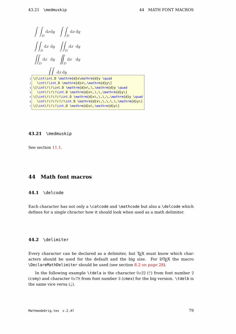
43.21 \medmuskip 44 MATH FONT MACROS

ˆ ˆD

dxdy

ˆ ˆD

dx dy

ˆ ˆD

dx dy

ˆˆD

dx dy

ˆˆD

dx dy

ˆD

dx dy

ˆˆD

dx dy

1 \[\int\int_D \mathrmdx\mathrmdy \quad2 \int\!\int_D \mathrmdx\,\mathrmdy\]3 \[\int\!\!\int_D \mathrmdx\,\,\mathrmdy \quad4 \int\!\!\!\int_D \mathrmdx\,\,\,\mathrmdy\]5 \[\int\!\!\!\!\int_D \mathrmdx\,\,\,\,\mathrmdy \quad6 \int\!\!\!\!\!\int_D \mathrmdx\,\,\,\,\,\mathrmdy\]7 \[\int\!\!\!\int_D \mathrmdx\,\mathrmdy\]

43.21 \medmuskip

See section 11.1.

44 Math font macros

44.1 \delcode

Each character has not only a \catcode and \mathcode but also a \delcode whichdefines for a single chracter how it should look when used as a math delimiter.

44.2 \delimiter

Every character can be declared as a delimiter, but TEX must know which char-acters should be used for the default and the big size. For LATEX the macro\DeclareMathDelimiter should be used (see section 8.2 on page 28).

In the following example \tdela is the character 0x22 (↑) from font number 2

(csmy) and character 0x78 from font number 3 (cmex) for the big version. \tdelb isthe same vice versa (↓).


44 MATH FONT MACROS 44.3 \displaystyle

↑x− y↓(x+ y) = x2 − y2

↑∞∑

n=0

1

2n↓2 = 4

x∞∑

n=0

1

2n

y

2

= 4

1 \def\tdela\delimiter"4222378\relax2 \def\tdelb\delimiter"5223379\relax3

4 $\tdela x-y\tdelb(x+y)=x^2-y^2$5

6 \[\tdela\sum_n=0^\infty 1\over2^n\tdelb^2 = 4\]7

8 \[\left\tdela\sum_n=0^\infty 1\over2^n\right\tdelb^2= 4\]

44.3 \displaystyle

See section 12 for an example.

44.4 \fam

When TEX switches into the math mode, it typesets everything using one of the 16possible families of fonts. \fam is an internal register where other macros can checkwhich font is the actual one. At the beginning TEX starts with \fam=-1.

\fam=-1 123abcABCαβγ\fam=0 123abcABCfffifl\fam=1 abcABCαβγ\fam=2 ∞∈3abcABC©\fam=3 ∐⟩∣∥\fam=4 123abcABC

\fam=5 123aABC

123abcABCfffifl(0)

123abcABCfffifl(13)

123abcABCfffifl(14)

123abcABC↑↓'(15)

123abcABCαβγ(−1)

abcABCαβγ()

1 $\mathrm123abcABC\alpha\beta\gamma (\the\fam)$\\[5pt]

2 $\mathbf123abcABC\alpha\beta\gamma (\the\fam)$\\[5pt]

3 $\mathit123abcABC\alpha\beta\gamma (\the\fam)$\\[5pt]

4 $\mathtt123abcABC\alpha\beta\gamma (\the\fam)$\\[5pt]

5 $\mathsf123abcABC\alpha\beta\gamma (\the\fam)$\\[5pt]

6 $\mathnormal123abcABC\alpha\beta\gamma (\the\fam)$

44.5 \mathaccent

Requires three parameter as one number, the class, the font family and the character.


44.6 \mathbin 44 MATH FONT MACROS

A1 \def\dA\mathaccent"7015\relax2 \Large $\dAA$

44.6 \mathbin

Declares a following character as a binary symbol with another spacing before andbehind such a symbol.

a|b a | b1 \Large2 $a|b \quad a\mathbin| b$

44.7 \mathchar

Declares a math character by three integer numbers as Parameters, giving its class,font family, and font position. In the following example \mathchar defines a characterof class 1 (big operators), font family 3 (math extension font) and number 58 (bigsum character).

a∞∑i=1

b a

∞∑

i=1

b

1 \Large2 $a\sum\limits_i=1^\infty b \quad3 a\mathchar"1358\limits_i=1^\infty b$

44.8 \mathchardef

This is in principle the same as \mathchar, it only allows to make such definitionspermanent.

a∞∑

i=1

√i+ 1

a∞∑i=1

√i+ 1

1 \bgroup2 \mathchardef\sum="13583 $a\sum\limits_i=1^\infty\sqrti+1$\\[5pt]4 \egroup5

6 $a\sum\limits_i=1^\infty\sqrti+1$

44.9 \mathchoice

Specifies specific subformula sizes for the 4 main styles: \displaystyle – \textstyle– \scriptstyle – \scriptscriptstyle.


44 MATH FONT MACROS 44.10 \mathclose

∞∑i=1

√i+1i2

1 \Large2 \def\myRule%3 \colorred%4 \mathchoice\rule2pt20pt\rule1pt10pt%5 \rule0.5pt5pt\rule0.25pt2.5pt%6 \mkern2mu7 $\myRule\sum\limits_\myRule i=1^\myRule\infty%8 \myRule\frac\myRule\sqrt\myRule i+1\myRule i^2$

44.10 \mathclose

Assigns class 5 (closing character) to the following parameter, which can hold asingle character or a subformula.

A : BC

: D

A:BC

:D1 \large2 $A:\fracBC:D$\\[5pt]3 $A\mathopen:\fracBC\mathclose: D $

44.11 \mathcode

A math font is far different from a text font. A lot of the characters has to be definedwith \mathcode, which defines the character with its class, font family and characternumber, e.g., \mathcode‘\<="313C. It defines the character “<” as a realtion symbol(class 3) from the font family 1 and the character number 0x3C, which is 60 decimal.

44.12 \mathop

Assigns class 1 (large operator) to the parameter, which can be a single character ora subformula.

A∞i=1

∞Ai=1

1 \[ A_i=1^\infty \]2 \[ \mathopA_i=1^\infty \]

44.13 \mathopen

Vice versa to \mathclose (see section 44.10).

44.14 \mathord

Assigns class 0 (ordinary character) to the following parameter, which can be a singlecharacter or a subformula.

y = f(x)

y=f(x)1 \large2 $y = f(x)$\\[5pt]3 $y \mathord= f(x)$


44.15 \mathpunct 44 MATH FONT MACROS

44.15 \mathpunct

Assigns class 6 (punctuation) to the following parameter, which can be a singlecharacter or a subformula (see section 11.4 for an example).

44.16 \mathrel

Assigns class 3 (relation) to the following parameter, which can be a single characteror a subformula.

x1ox2ox3

x1 o x2 o x31 \large2 $x_1 o x_2 o x_3$\\[5pt]3 $x_1\mathrel o x_2\mathrel o x_3$

44.17 \scriptfont

Specifies the scriptstyle font (used for super/subscript) for a family.

A1 A11 $A_1$2 \font\tenxii=cmr123 \scriptfont0=\tenxii4 $A_1$

44.18 \scriptscriptfont

Specifies the scriptscriptstyle font for a family.

44.19 \scriptscriptstyle

Selects scriptscript style for the following characters.

44.20 \scriptstyle

Selects script style for the following characters.

44.21 \skew

Especially for italic characters double accents are often misplaced. \skew has threearguments

horizontal shift: A value in math units for the additional shift of the accent.

the accent: The symbol which is placed above the character.

the character: This is in general a single character, but can also include itself anaccent.

AMSmath redefines the setting of double accents. This is the reason why thereare only a few cases where someone has to use \skew when the package amsmath isloaded, like in this document.


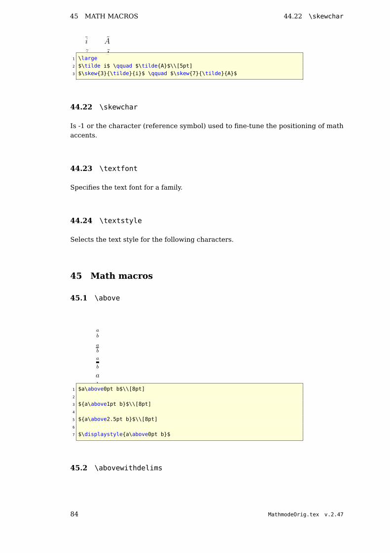
45 MATH MACROS 44.22 \skewchar

i A

i A1 \large2 $\tilde i$ \qquad $\tildeA$\\[5pt]3 $\skew3\tildei$ \qquad $\skew7\tildeA$

44.22 \skewchar

Is -1 or the character (reference symbol) used to fine-tune the positioning of mathaccents.

44.23 \textfont

Specifies the text font for a family.

44.24 \textstyle

Selects the text style for the following characters.

45 Math macros

45.1 \above

ab

ab

a

b

a

b1 $a\above0pt b$\\[8pt]2

3 $a\above1pt b$\\[8pt]4

5 $a\above2.5pt b$\\[8pt]6

7 $\displaystylea\above0pt b$

45.2 \abovewithdelims


45.3 \atop 45 MATH MACROS

(ab

)

ab

)

[ab

]

a

b1 $a\abovewithdelims()0pt b$\\[8pt]2

3 \def\fdelimA\abovewithdelims\)1.0pt4 $a\fdelimA b$\\[8pt]5

6 \def\fdelimB\abovewithdelims[]2.0pt7 $a\fdelimB b$\\[8pt]8

9 \def\fdelimC\abovewithdelims\.0pt10 $\displaystylea\fdelimC b$

45.3 \atop

ab

(nk ) = n!k!(n−k)!

a

b1 $a\atop b$\\[8pt]2

3 $(n \atop k) = n!\above1pt k!(n-k)!$\\[8pt]4

5 $\displaystylea\atop b$

45.4 \atopwithdelims

(ab

)

(nk

)= n!

k!(n−k)!

a

b1 $a\atopwithdelims() b$\\[8pt]2

3 $n \atopwithdelims() k = n!\above1pt k!(n-k)!$\\[8pt]4

5 $\displaystylea\atopwithdelims\. b$

45.5 \displaylimits

Resets the conventions for using limits with operators to the standard for the usedenvironment.

45.6 \eqno

Puts an equation number at the right margin, the parameter can hold anything.\eqno places only the parameter, but doesn’t increase any equation counter.


45 MATH MACROS 45.7 \everydisplay

y = f(x) (A12)1 \[ y=f(x) \eqno(A12) \]

45.7 \everydisplay

Inserts the parameter at the start of every switch to display math mode.

f(x) =

ˆsinx

xdx

g(x) =

ˆsin2 x

x2dx

1 \everydisplay\colorred2 3 \[ f(x) = \int \frac\sin xx\,\mathrmdx \]4 \[ g(x) = \int \frac\sin^2 xx^2\,\mathrmdx \]

45.8 \everymath

Same as \everydisplay, but now for the inline mode. In the following example thedisplaystyle is used (besides using color red) for every inline math expression.

f(x) =

ˆsinx

xdx

Instead ofsinx

xnow with

cosx

x:

g(x) =

ˆcosx

xdx

1 \everymath\colorred%2 \displaystyle3 \[ f(x) = \int \frac\sin xx\,\mathrmdx \]4 Instead of $\frac\sin xx$5 now with $\frac\cos xx$:6 \[ g(x) = \int \frac\cos xx\,\mathrmdx \]

Pay attention for side effects on footnotes and other macros which use the mathmode for superscript and other math related modes. In this case you’ll get thefootnotes also in red.

45.9 \left

TEX calculates the size of the following delimiter needed at the left side of a formula.Requires an additional right.

45.10 \leqno

Vice versa to \eqno (see section 45.6 on the previous page).


45.11 \limits 45 MATH MACROS

45.11 \limits

Typesets limits above and/or below operators (see section 6 on page 22).

45.12 \mathinner

Defines the following parameter as subformula.

45.13 \nolimits

The opposite of \limits, instead of above/below limits are placed to the right oflarge operators (class 1).

45.14 \over

Is equivalent to the fraction macro of LATEX and equivalent to the \overwithdelims,see section 45.16.

ab

mna+b

mn

a+ b1 $ a\over b \qquad m\over n\overa+b $2 \[ m\over n\overa+b \]

45.15 \overline

Puts a line over the following character or subformula and has the same problemswith different heights as underlines (see section 45.19).

x+ y = z

x+A = z

x+A = z1 $\overlinex+\overliney=\overlinez$\\2 \let\ol\overline3 $ \olx + \olA = \olz $\\[5pt]4 \def\yPh\vphantomA5 $ \olx\yPh + \olA = \olz\yPh $

45.16 \overwithdelims

Is a generalized fraction command with preset fraction bar thickness.

(ab

) [ mna+b

]

mn

a+ b1 $ a\overwithdelims() b \qquad m\over n\overwithdelims[]a+b

$2 \[ m\over n\overwithdelims\.a+b \]


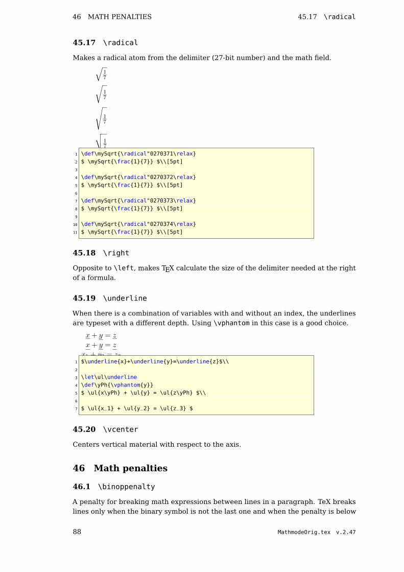
46 MATH PENALTIES 45.17 \radical

45.17 \radical

Makes a radical atom from the delimiter (27-bit number) and the math field.√

17

√17

√17

√√17

1 \def\mySqrt\radical"0270371\relax2 $ \mySqrt\frac17 $\\[5pt]3



10 \def\mySqrt\radical"0270374\relax11 $ \mySqrt\frac17 $\\[5pt]

45.18 \right

Opposite to \left, makes TEX calculate the size of the delimiter needed at the rightof a formula.

45.19 \underline

When there is a combination of variables with and without an index, the underlinesare typeset with a different depth. Using \vphantom in this case is a good choice.

x+ y = z

x+ y = z

x1 + y2 = z31 $\underlinex+\underliney=\underlinez$\\2

3 \let\ul\underline4 \def\yPh\vphantomy5 $ \ulx\yPh + \uly = \ulz\yPh $\\6

7 $ \ulx_1 + \uly_2 = \ulz_3 $

45.20 \vcenter

Centers vertical material with respect to the axis.

46 Math penalties

46.1 \binoppenalty

A penalty for breaking math expressions between lines in a paragraph. TeX breakslines only when the binary symbol is not the last one and when the penalty is below


46.2 \displaywidowpenalty 46 MATH PENALTIES

10,000.

46.2 \displaywidowpenalty

The penalty which is added after the penultimate line immediately preceeding adisplay math formula.

46.3 \postdisplaypenalty

Is added immediately after a math display ends.

46.4 \predisplaypenalty

Is added immediately before a math display starts.

46.5 \relpenalty

The penalty for a line break after a relation symbol (if a break is possible).


Math packages

Part IV

Other packages

The following sections are not a replacement for the package documentation!

47 List of available math packages

accents alphalph amsart amsbookamsbsy amscd amscls amsfontsamslatex amsltx11 amsmath amspptamsppt1 amsproc amssym (plain TeX) amssymb (LaTeX)amstex (Plain TeX) amstext amsthm bez123bitfield brclc breqn cancelcases comma datenumber diagxydoublestroke easyeqn easybmat easymateqnarray esvect fixmath ftlpointicomma leftidx mathdots mathtoolsmathematica mil3 mtbe Nathnumprint random romannum TeXaide

The following examples depend on the listed versions of the packages:

amsopn.sty 1999/12/14 v2.01 operator namesbm.sty 1999/07/05 v1.0g Bold Symbol Support (DPC/FMi)

empheq.sty 2007/12/03 v2.12 Emphasizing equations (MH)amscd.sty 1999/11/29 v2.0

accents.sty 2000/08/06 v1.2 Math Accent Toolsframed.sty 2007/10/04 v 0.95: framed or shaded text with page breaks

pstricks.sty 2004/05/06 v0.2k LaTeX wrapper for ‘PSTricks’ (RN,HV)pstricks.tex 2003/03/07 v97 patch 15 ‘PSTricks’ (tvz)pst-node.tex 2008/11/26 v1.01 PSTricks package for nodes (tvz,hv)delarray.sty 1994/03/14 v1.01 array delimiter package (DPC)

xypic.sty 1999/02/16 Xy-pic version 3.7exscale.eps Graphic file (type veps)

47.1 accents

If you want to write for example an underlined M, then you can do it by

\underline$M$ M

\underbar$M$ M

\underaccent\barM¯M

As seen, there is no difference between \underline and \underbar. For somereasons it may be better to use the accent package with the \underaccents macro.

47.2 amscd – commutative diagrams

The amscd package is part of the AMSmath bundle or available at CTAN27 and has nooptions for the \usepackage command. amscd does not support diagonal arrows but

27CTAN://macros/latex/required/amslatex/math/amscd.dtx


http://www.dante.de/CTAN/help/Catalogue/entries/accents.html

http://www.dante.de/CTAN/help/Catalogue/entries/alphalph.html

http://www.dante.de/CTAN/help/Catalogue/entries/amsart.html

http://www.dante.de/CTAN/help/Catalogue/entries/amsbook.html

http://www.dante.de/CTAN//help/Catalogue/entries/amsbsy.html

http://www.dante.de/CTAN//help/Catalogue/entries/amscd.html

http://www.dante.de/CTAN//help/Catalogue/entries/amscls.html

http://www.dante.de/CTAN//help/Catalogue/entries/amsfonts.html

http://www.dante.de/CTAN//help/Catalogue/entries/amslatex.html

http://www.dante.de/CTAN//help/Catalogue/entries/amsltx11.html

http://www.dante.de/CTAN//help/Catalogue/entries/amsmath.html

http://www.dante.de/CTAN//help/Catalogue/entries/amsppt.html

http://www.dante.de/CTAN//help/Catalogue/entries/amsppt1.html

http://www.dante.de/CTAN//help/Catalogue/entries/amsproc.html

http://www.dante.de/CTAN//help/Catalogue/entries/amssym.html

http://www.dante.de/CTAN//help/Catalogue/entries/amssymb.html

http://www.dante.de/CTAN//help/Catalogue/entries/amstex.html

http://www.dante.de/CTAN//help/Catalogue/entries/amstext.html

http://www.dante.de/CTAN//help/Catalogue/entries/amsthm.html

http://www.dante.de/CTAN//help/Catalogue/entries/bez123.html

http://www.dante.de/CTAN//help/Catalogue/entries/bitfield.html

http://www.dante.de/CTAN//help/Catalogue/entries/brclc.html

http://www.dante.de/CTAN//help/Catalogue/entries/breqn.html

http://www.dante.de/CTAN//help/Catalogue/entries/cancel.html

http://www.dante.de/CTAN//help/Catalogue/entries/cases.html

http://www.dante.de/CTAN//help/Catalogue/entries/comma.html

http://www.dante.de/CTAN//help/Catalogue/entries/datenumber.html

http://www.dante.de/CTAN//help/Catalogue/entries/diagxy.html

http://www.dante.de/CTAN//help/Catalogue/entries/doublestroke.html

http://www.dante.de/CTAN//help/Catalogue/entries/easyeqn.html

http://www.dante.de/CTAN//help/Catalogue/entries/easybmat.html

http://www.dante.de/CTAN//help/Catalogue/entries/easymat.html

http://www.dante.de/CTAN//help/Catalogue/entries/eqnarray.html

http://www.dante.de/CTAN//help/Catalogue/entries/esvect.html

http://www.dante.de/CTAN//help/Catalogue/entries/fixmath.html

http://www.dante.de/CTAN//help/Catalogue/entries/fltpoint.html

http://www.dante.de/CTAN//help/Catalogue/entries/icomma.html

http://www.dante.de/CTAN//help/Catalogue/entries/leftidx.html

http://www.dante.de/CTAN//help/Catalogue/entries/mathdots.html

http://www.dante.de/CTAN//help/Catalogue/entries/mathtools.html

http://www.dante.de/CTAN//help/Catalogue/entries/mathematica.html

http://www.dante.de/CTAN//help/Catalogue/entries/mil3.html

http://www.dante.de/CTAN//help/Catalogue/entries/mtbe.html

http://www.dante.de/CTAN//help/Catalogue/entries/nath.html

http://www.dante.de/CTAN//help/Catalogue/entries/numprint.html

http://www.dante.de/CTAN//help/Catalogue/entries/random.html

http://www.dante.de/CTAN//help/Catalogue/entries/romannum.html

http://www.dante.de/CTAN//help/Catalogue/entries/texaide.html

http://www.ctan.org/tex-archive/macros/latex/required/amslatex/math/amscd.dtx

47.3 amsopn Math packages

is much easier to handle than the complex pstricks package or the xypic package.On the other hand simple diagrams can be written with the array environment orlook at [23].

R× S × T restriction−−−−−−→ S × Tproj

yyproj

R× S ←−−−−−inclusion

S

1 \[2 \beginCD3 R\times S\times T @>\textrestriction>> S\times T \\4 @VprojVV @VVprojV \\5 R\times S @<<\textinclusion< S6 \endCD7 \]

47.3 amsopn

With the amsopn package it is very easy to declare new math operators, which arewritten in upright mode:

Ress=p

versus Ress=p

1 \documentclass[10pt]article2 \usepackageamsmath3 \usepackageamsopn4 \DeclareMathOperator\ResRes5 \begindocument6 $\undersets=pRes\quad\undersets=p\Res$7 \enddocument

Table 20 shows the predefined operatornames of amsopn.

\arccos arccos \arcsin arcsin \arctan arctan\arg arg \cos cos \cosh cosh\cot cot \coth coth \csc csc\deg deg \det det \dim dim\exp exp \gcd gcd \hom hom\inf inf \injlim inj lim \ker ker\lg lg \lim lim \liminf lim inf\limsup lim sup \ln ln \log log\max max \min min \Pr Pr\projlim proj lim \sec sec \sin sin\sinh sinh \sup sup \tan tan\tanh tanh

Table 20: The predefined operators of amsopn.sty

47.4 bigdel

This is a very useful package together with the multirow package. In the followingexample we need additional parentheses for a different number of rows. This is alsopossible with the array environment, but not as easy as with the bigdelim package.


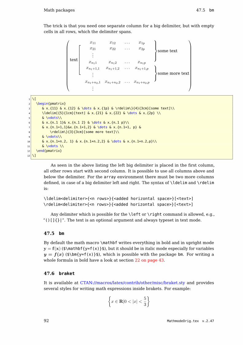
Math packages 47.5 bm

The trick is that you need one separate column for a big delimiter, but with emptycells in all rows, which the delimiter spans.

x11 x12 . . . x1p

some text

text

x21 x22 . . . x2p...

xn11 xn12 . . . xn1p

xn1+1,1 xn1+1,2 . . . xn1+1,psome more text...

xn1+n2,1 xn1+n2,2 . . . xn1+n2,p...

1 \[2 \beginpmatrix3 & x_11 & x_12 & \dots & x_1p & \rdelim\43cm[some text]\\4 \ldelim[51cm[text] & x_21 & x_22 & \dots & x_2p \\5 & \vdots\\6 & x_n_1 1& x_n_1 2 & \dots & x_n_1 p\\7 & x_n_1+1,1&x_n_1+1,2 & \dots & x_n_1+1, p &8 \rdelim\33cm[some more text]\\9 & \vdots\\

10 & x_n_1+n_2, 1 & x_n_1+n_2,2 & \dots & x_n_1+n_2,p\\11 & \vdots \\12 \endpmatrix13 \]

As seen in the above listing the left big delimiter is placed in the first column,all other rows start with second column. It is possible to use all columns above andbelow the delimiter. For the array environment there must be two more columnsdefined, in case of a big delimiter left and right. The syntax of \ldelim and \rdelimis:

\ldelim<delimiter><n rows><added horizontal space>[<text>]\rdelim<delimiter><n rows><added horizontal space>[<text>]

Any delimiter which is possible for the \left or \right command is allowed, e.g.,“()[]|”. The text is an optional argument and always typeset in text mode.

47.5 bm

By default the math macro \mathbf writes everything in bold and in upright modey = f(x) ($\mathbfy=f(x)$), but it should be in italic mode especially for variablesy = f(x) ($\bmy=f(x)$), which is possible with the package bm. For writing awhole formula in bold have a look at section 22 on page 43.

47.6 braket

It is available at CTAN://macros/latex/contrib/other/misc/braket.sty and providesseveral styles for writing math expressions inside brakets. For example:

x ∈ R|0 < |x| < 5

3


http://www.ctan.org/tex-archive/macros/latex/contrib/other/misc/braket.sty

47.6 braket Math packages

1 \[ \left\ x\in\mathbfR | 0<|x|<\frac53\right\ \]

looks not quite right and it is not really easy to get the first vertical line in the samesize as the outer braces. Some solution may be using \vphantom:

x ∈ R

∣∣∣∣ 0 < |x| < 5

3

1 \[2 \left\\vphantom\frac53x\in\mathbfR \right|\left. 0<|x|<\frac53\right\3 \]

The package braket has the macros

1 \Bra<math expression>2 \Ket<math expression>3 \Braket<math expression>4 \Set<math expression>

and the same with a leading lower letter, which are not really interesting.

⟨x ∈ R|0 < |x| < 5

3

∣∣∣∣∣∣∣∣x ∈ R|0 < |x| < 5

3

⟩

⟨x ∈ R

∣∣∣∣ 0 <∣∣∣∣x∣∣∣∣<

5

3

⟩

⟨x ∈ R

∣∣∣∣ 0 < |x| <5

3

⟩

x ∈ R

∣∣∣∣ 0 < |x| < 5

3

1 \[ \Brax\in\mathbfR | 0<|x|<\frac53 \]2 \[ \Ketx\in\mathbfR | 0<|x|<\frac53 \]3 \[ \Braketx\in\mathbfR | 0<|x|<\frac53 \]4 \[ \Braketx\in\mathbfR | 0<\vert x\vert <\frac53 \]5 \[ \Setx\in\mathbfR | 0<|x|<\frac53 \]

The difference between the \Set and the \Braket macro is the handling of thevertical lines. In \Set only the first one gets the same size as the braces and in\Braket all.

⟨φ

∣∣∣∣∂2

∂t2

∣∣∣∣ψ⟩

φ

∣∣∣∣∂2

∂t2|ψ

1 \[\Braket\phi | \frac\partial^2\partial t^2 | \psi\]2 \[\Set\phi | \frac\partial^2\partial t^2 | \psi\]

\Bra and \Ket do nothing with the inner vertical lines.


Math packages 47.7 cancel

47.7 cancel

This is a nice package for canceling anything in mathmode with a slash, backslash ora X. To get a horizontal line we can define an additional macro called \hcancel withan optional argument for the line color (requires package color):

1 \newcommand\hcancel[2][black]\setbox0=\hbox#2%2 \rlap\raisebox.45\ht0\textcolor#1\rule\wd01pt#2

It is no problem to redefine the \cancel macros to get also colored lines. Ahorizontal line for single characters is also decribed in section 14 on page 37.

\cancel: f(x) =

(x2 + 1

)

(x− 1)

(x− 1)(x+ 1)

\bcancel: A3hhhhh1234567

\xcancel: A3 (((((hhhhh1234567

\hcancel: 3 1234567

1 $f(x)=\dfrac\left(x^2+1\right)\cancel(x-1)\cancel(x-1)(x+1)$\\[0.5cm]2 $\bcancel3\qquad\bcancel1234567$\\[0.5cm]3 $\xcancel3\qquad\xcancel1234567$\\[0.5cm]4 $\hcancel3\qquad\hcancel[red]1234567$

47.8 cool

The cool package defines a lot of special mathematical expressions to use them bythe macro name. The following list shows only some of them, for more informationslook at the example file, which comes with the package.

\Sinx sin(x)

\Cosx cos(x)

\Tanx tan(x)

\Cscx csc(x)

\Secx sec(x)

\Cotx cot(x)

\StyleArcTrig=inverse (default)

\ArcSinx sin−1(x)

\ArcCosx cos−1(x)

\ArcTanx tan−1(x)

\StyleArcTrig=arc

\ArcSinx arcsin(x)

\ArcCosx arccos(x)

\ArcTanx arctan(x)

\ArcCscx csc−1(x)

\ArcSecx sec−1(x)

\ArcCotx cot−1(x)


47.9 delarray Math packages

\Factorialn n!

\DblFactorialn n!!

\Binomialnk

(n

k

)

\Multinomial1,2,3,4 (i1 + . . .+ in; i1, . . . , in)

\GammaFuncx Γ(x)

\IncGammaax Γ(a, x)

\GenIncGammaaxy Γ(a, x, y)

\RegIncGammaax Q(a, x)

\RegIncGammaInvax Q−1(a, x)

\GenRegIncGammaaxy Q(a, x, y)

\GenRegIncGammaInvaxy Q−1(a, x, y)

\Pochhammeran (a)n\LogGammax logΓ(x)

\Hypergeometric00x 0F0(; ;x)

\Hypergeometric01bx 0F1(; b;x)

\RegHypergeometric00x 0F 0(; ;x)

\RegHypergeometric01bx 0F 1(; b;x)

\MeijerG[a,b]npmqx

Gm,np,q

(x

∣∣∣∣a1, . . . , an, an+1, . . . , apb1, . . . , bm, bm+1, . . . , bq

)

\MeijerG1,2,3,45,63,6,912,15,18,21,24x

G3,46,8

(x

∣∣∣∣1, 2, 3, 4, 5, 6

3, 6, 9, 12, 15, 18, 21, 24

)

\RiemannZetas ζ(s)

\Zetas ζ(s)

\HurwitzZetasa ζ(s, a)

\Zetas,a ζ(s, a)

\RiemannSiegelThetax ϑ(x)

\RiemannSiegelZx Z(x)

\StieltjesGamman γn

\MathieuCaqz Ce(a, q, z)

\MathieuSaqz Se(a, q, z)

\MathieuCharacteristicArq ar(q)

\MathieuCharisticArq ar(q)

\MathieuCharacteristicBrq br(q)

\MathieuCharisticBrq br(q)

\MathieuCharacteristicExponentaq r(a, q)

\MathieuCharisticExpaq r(a, q)

47.9 delarray

Package delarray28 supports different delimiters which are defined together withthe beginning of an array:

28CTAN://macros/latex/required/tools/delarray.dtx


http://www.ctan.org/tex-archive/macros/latex/required/tools/delarray.dtx

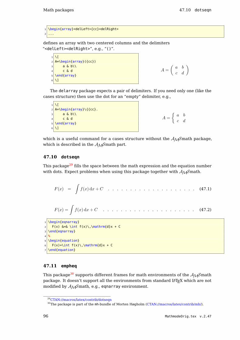
Math packages 47.10 dotseqn

1 \beginarray<delLeft>cc<delRight>2 ...

defines an array with two centered columns and the delimiters“<delLeft><delRight>”, e.g., “()”.

1 \[2 A=\beginarray(cc)3 a & b\\4 c & d5 \endarray6 \]

A =

(a b

c d

)

The delarray package expects a pair of delimiters. If you need only one (like thecases structure) then use the dot for an “empty” delimiter, e.g.,

1 \[2 A=\beginarray\cc.3 a & b\\4 c & d5 \endarray6 \]

A =

a b

c d

which is a useful command for a cases structure without the AMSmath package,which is described in the AMSmath part.

47.10 dotseqn

This package29 fills the space between the math expression and the equation numberwith dots. Expect problems when using this package together with AMSmath.

F (x) =

ˆf(x) dx+ C . . . . . . . . . . . . . . . . . . . . (47.1)

F (x) =

ˆf(x) dx+ C . . . . . . . . . . . . . . . . . . . . . (47.2)

1 \begineqnarray2 F(x) &=& \int f(x)\,\mathrmdx + C3 \endeqnarray4 %5 \beginequation6 F(x)=\int f(x)\,\mathrmdx + C7 \endequation

47.11 empheq

This package30 supports different frames for math environments of the AMSmathpackage. It doesn’t support all the environments from standard LATEX which are notmodified by AMSmath, e.g., eqnarray environment.

29CTAN://macros/latex/contrib/dotseqn30The package is part of the mh-bundle of Morten Høgholm (CTAN://macros/latex/contrib/mh/).


http://www.ctan.org/tex-archive/macros/latex/contrib/dotseqn/

http://www.ctan.org/tex-archive/macros/latex/contrib/mh/

47.12 esint Math packages

With the optional argument of the empheq environment the preferred box typecan be specified. A simple one is \fbox

f(x) =

ˆ ∞1

1

x2dx = 1 (47.3)

1 \beginempheq[box=\fbox]align2 f(x)=\int_1^\infty\frac1x^2\,\mathrmdx=13 \endempheq

The same is possible with the macro \colorbox:

f(x) =

ˆ ∞1

1

x2dx = 1 (47.4)

1 \beginempheq[box=\fboxsep=10pt\colorboxyellow]align2 f(x)=\int_1^\infty\frac1x^2\,\mathrmdx=13 \endempheq

The key box can hold any possible LATEX command sequence. Boxing subequationsis also no problem, the empheq environment works in the same way:

f(x) =

ˆ ∞1

1

x1dx = 1

f(x) =

ˆ ∞2

1

x2dx = 0.25

(47.5a)

(47.5b)

1 \beginsubequations2 \beginempheq[box=\fboxsep=10pt\colorboxcyan]align3 f(x) & =\int_1^\infty\frac1x^2\,\mathrmdx=1\\4 f(x) & =\int_2^\infty\frac1x^2\,\mathrmdx=0.255 \endempheq6 \endsubequations

For more information on empheq package have a look at the documentation of thepackage which is available at any CTAN server.

47.12 esint

This is a very useful package when you want nice double or triple integral or curveintegral symbols. The ones from the wasysym package31 are not the best. esint32

supports the following symbols:

\int :

ˆ(47.6)

\iint :

¨(47.7)

\iiintop :

˚(47.8)

31CTAN://macros/latex/contrib/wasysym/32CTAN://macros/latex/contrib/esint/ CTAN://fonts/ps-type1/esint/


http://www.ctan.org/tex-archive/macros/latex/contrib/wasysym/

http://www.ctan.org/tex-archive/macros/latex/contrib/esint/

http://www.ctan.org/tex-archive/fonts/ps-type1/esint/

Math packages 47.13 eucal and euscript

\iiiintop :

˘(47.9)

\dotsintop :

˙(47.10)

\ointop :

˛(47.11)

\oiint :

‹(47.12)

\sqint :

“(47.13)

\sqiint :

„(47.14)

\ointctrclockwise :

‰(47.15)

\ointclockwise :

(47.16)

\varointclockwise :

fi(47.17)

\varointctrclockwise :

ffi(47.18)

\fint :

(47.19)

\varoiint :

"(47.20)

\landupint :

$(47.21)

\landdownint :

&(47.22)

47.13 eucal and euscript

These packages should be part of your local TEX installation, because they comewith the AMSmath packages. Otherwise get them from CTAN33. They support ascriptwriting of only uppercase letters:

\mathscr... ABCDEFGHIJKLMNOPQRSTUVWXYZ

Read the documentation for the interdependence to the \mathcal command. Forthe above example the package eucal was loaded with the option mathscr.

47.14 exscale

The following formula is written with the default fontsize where everything looksmore or less well:

ˆ +1

−1

f(x)√1− x2

dx ≈ π

n

n∑

i=1

f

(cos

(2i− 1

2n

))

Writing the same with the fontsize \huge gives a surprising result, which belongsto the historical development of LATEX, the \int and \sum symbols are not stretched.This extreme fontsize is often needed for slides and not only written “just for fun”.

33CTAN://fonts/amsfonts/latex/euscript.sty


http://www.ctan.org/tex-archive/fonts/amsfonts/latex/euscript.sty

47.15 mathtools Math packages

∫ +1−1

f (x)√

1− x2dx ≈

π

n

n∑

i=1f

cos

2i− 1

2n

Using the exscale package34 package, which should be part of any local TEXinstallation, all symbols get the right size.ˆ +1

−1

f (x)√1− x2

dx ≈ π

n

n∑

i=1

f

(cos

(2i− 1

2n

))

47.15 mathtools

This package comes with a lot of additional features for typesetting math code.Sometimes it is useful when only such equations are numbered which are referencedin the text. This is possible with the switch \showonlyrefs.

Matrices are set by default with a centered horizontal alignment, which is oftennot the best way. The mathtools package provides a starred version of the matrixenvironments which allow an optional argument for the horizontal alignment:

1 −1 0

−1 1 −1

1 −1 0

−11 11 −11

1 \[2 \beginpmatrix*[r]3 1 & -1 & 0 \\4 -1 & 1 & -1 \\5 1 & -1 & 0 \\6 -11 & 11 &-11 \\7 \endpmatrix*8 \]

mathtools also provides some more environments for setting equations. Veryinteresting is the lgathered environment, which allows to typeset a formula in thefollowing way:

34CTAN://macros/latex/base/


http://www.ctan.org/tex-archive/macros/latex/base/

Math packages 47.16 nicefrac

x = a+ b+ c

d+ e+ f + g + h

i+ j + k

(47.23)

1 \beginalign2 x &=3 \beginlgathered[t]4 a + b + c \\5 d + e +6 \!\begingathered[t]7 f + g + h \\8 i + j + k9 \endgathered

10 \endlgathered11 \endalign

The \! revokes the internal horizontal space in front of the gathered environ-ment.

47.16 nicefrac

Typesetting fractions in the inline mode is often a bad choice, the vertical spacingincreases in fact of the fraction. The nicefrac package defines the macro \nicefrac,which is used in the same way as the \frac command, but it typesets the fractionwith a less height: 2/3 \nicefrac23. The package is part of the units packagebundle and can be found in the directory of units.

47.17 relsize

Often consecutives math operators are used, like two sum symbols, e.g.,

∑ n∑

i=1

i2

As seen the sums are of the same size. To increase the first operator size, someonecan use the \scalebox macro from package graphicx environment and write an ownmacro \Sum, e.g.,

1 \def\Sum\ensuremath\mathop\scalebox1.2$\displaystyle\sum$2 \[ \Sum_j=1\sum_i=1^\infty i \]

∑

j=1

∞∑

i=1

i

Another solution is to use the relsize package35 together with the exscale one.relsize defines a useful macro \mathlarger:

∑ n∑

i=1

i2

1 \[ \mathlarger\sum\sum_i=1^n i^2 \]

35CTAN://macros/latex/ltxmisc/


http://www.ctan.org/tex-archive/macros/latex/ltxmisc/

47.18 xypic Math packages

47.18 xypic

The \xymatrix macro is part of the xypic package36 which can be loaded withseveral options which are not so important here.37.

A B C

D E F

G H I

(47.24)

This matrix was created with

1 \[2 \xymatrix A\POS [];[d]**\dir ~,[];[dr]**\dir - & B & C\\3 D & E\POS [];[l]**\dir .,[];[r]**\dir ~ & F\POS [];[dl]**\dir ~\\4 G & H & I5 \]

36CTAN://macros/generic/diagrams/xypic/xy-3.7/37For more information look at the package documentation or the package xy itself, which is often

saved in /usr/share/texmf/tex/generic


http://www.ctan.org/tex-archive/support/latex2html/

49 LATIN MODERN

Part V

Math fonts

Typesetting text and math is far different. There exist a lot of free text fonts withoutadditional math characters. This is the reason why we have to buy a commercialmath font, e. g. Palatino (pamath) or Helvetica (hvmath), or to combine the free textfont with another free math font.

48 Computer modern

This is the default font, designed by Knuth. For the PDF output the Type 1 fontscm-super and BlueSky were used.

Theorem 1 (Residuum). Für eine in einer punktierten Kreisscheibe D\aanalytische Funktion f definiert man das Residuum im Punkt a als

Resz=a

f(z) = Resaf =

12πi

∫C

f(z) dz ,

wobei C ⊂ D\a ein geschlossener Weg mit n(C, a) = 1 ist (z.B. ein entgegendem Uhrzeigersinn durchlaufener Kreis).

AΛ∆∇BCDΣEFΓGHIJKLMNOΘΩfPΦΠΞQRSTUVWXYΥΨZaαbβc∂dδeεεfζξgγh~ιiıjkκκl`λmnηθϑoσςφϕ℘pρ%qrstτπuµνvυwω$xχyψz∞ ∝ ∅∅dð

49 Latin modern

This is the new designed font which comes with an own Type 1 version.lm

Theorem 1 (Residuum). Für eine in einer punktierten Kreisscheibe D\aanalytische Funktion f definiert man das Residuum im Punkt a als

Resz=a

f(z) = Resaf =

12πi

∫C

f(z) dz ,


AΛ∆∇BCDΣEFΓGHIJKLMNOΘΩfPΦΠΞQRSTUVWXYΥΨZaαbβc∂dδeεεfζξgγh~ιiıjkκκl`λmnηθϑoσςφϕ℘pρ%qrstτπuµνvυwω$xχyψz∞ ∝ ∅∅dð


51 PALATINO – MICROIMP

50 Palatino

There is a free package mathpazo.mathpazo

Theorem 1 (Residuum). Für eine in einer punktierten Kreisscheibe D\a ana-lytische Funktion f definiert man das Residuum im Punkt a als

Resz=a

f (z) = Resa

f =1

2πi

∫C

f (z) dz ,


AΛ∆∇BCDΣEFΓGHIJKLMNOΘΩfPΦΠΞQRSTUVWXYΥΨZaαbβc∂dδeεε f ζξgγhhιiıjkκκl`λmnηθϑoσςφϕ℘pρ$qrstτπuµνvυwωvxχyψz∞ ∝ ∅∅dð

51 Palatino – microimp

There is the package pamath for the nonfree palatino font.mathpazo

Theorem 1 (Residuum). Für eine in einer punktierten Kreisscheibe D\a ana-lytische Funktion f definiert man das Residuum im Punkt a als

Resz=a

f(z) = Resaf =

12πi

∫C

f(z)dz ,


AΛ∆∇BCDΣEFΓGHIJKLMNOΘΩfPΦΠΞQRSTUVWXYΥΨZaαbβc∂dδeεεfζξgγhħιiıjkκκl`λmnηθϑoσςφϕ℘pρ%qrstτπuµνvυwω$xχyψz∞ ∝ ∅∅dð


53 MINION

52 cmbright

Theorem 1 (Residuum). Für eine in einer punktierten Kreisscheibe D\a analytis-che Funktion f definiert man das Residuum im Punkt a als

Resz=a

f (z) = Resaf =

1

2πi

∫C

f (z) dz ,

wobei C ⊂ D\a ein geschlossener Weg mit n(C, a) = 1 ist (z.B. ein entgegen demUhrzeigersinn durchlaufener Kreis).

AΛ∆∇BCDΣEFΓGHIJKLMNOΘΩfPΦΠΞQRSTUVWXYΥΨZaαbβc∂dδeεεf ζξgγh~ιi ıj kκκ l `λmnηθϑoσςφϕ℘pρ%qrstτπuµνvυwω$xχyψz∞ ∝ ∅∅dð

53 minion

¿eorem 1 (Residuum). Für eine in einer punktierten Kreisscheibe Da analytischeFunktion f deniert man das Residuum im Punkt a als

Resz=a

f(z) = Resaf =

12πi ∫

C

f(z)dz ,

wobei C ⊂ Da ein geschlossener Weg mit n(C,a) = 1 ist (z.B. ein entgegen demUhrzeigersinn durchlaufener Kreis).

AΛ∆∇BCDΣEFΓGHIJKLMNOΘΩΩPΦΠΞQRSTUVWXYΥΨZaαbβc∂dδeєεfζξgγhħħιiıjȷkκϰlℓλmnηθϑoσςϕφ³pρρqrstτπuµνvυwωϖxχyψzª ggdðэ


54 INTEGRAL SYMBOLS

Part VI

Special symbols

In this section only those symbols are defined, which are not part of the list ofall available symbols: CTAN://info/symbols/comprehensive/symbols-a4.pdf. Withfontmath.ltx LATEX itself defines the following special symbols for using insidemath:

Name Meaning\mathparagraph ¶\mathsection §\mathdollar $\mathsterling £\mathunderscore\mathellipsis . . .

Table 21: Predefined math symbols from fontmath.ltx

54 Integral symbols

Name Symbol

\dashint −\ddashint =

\clockint

\counterint

For all new integral symbols limits can be used in the usual way:

=

ˆ0

1 = −ˆ

10 <

∞

−∞

= ˆ

ˆA

(54.1)

1 \ddashint_01=\dashint_10<\oint\limits_-\infty^\infty = \clockint\counterint_A

Put the following definitions into the preamble to use one or all of these newintegral symbols.

1 \def\Xint#1\mathchoice2 \XXint\displaystyle\textstyle#1%3 \XXint\textstyle\scriptstyle#1%4 \XXint\scriptstyle\scriptscriptstyle#1%5 \XXint\scriptscriptstyle\scriptscriptstyle#1%6 \!\int7 \def\XXint#1#2#3\setbox0=\hbox$#1#2#3\int$8 \vcenter\hbox$#2#3$\kern-.5\wd09 \def\ddashint\Xint=

10 \def\dashint\Xint-11 \def\clockint\Xint\circlearrowright % GOOD!12 \def\counterint\Xint\rotcirclearrowleft % Good for Computer Modern!13 \def\rotcirclearrowleft\mathpalette\RotLSymbol-30\circlearrowleft14 \def\RotLSymbol#1#2#3\rotatebox[origin=c]#1$#2#3$


http://www.ctan.org/tex-archive/info/symbols/comprehensive/symbols-a4.pdf

56 BIJECTIVE MAPPING ARROW

55 Harpoons

LATEX knows no stretchable harpoon symbols, like \xrightarrow. The following codedefines several harpoon symbols.\xrightharpoondown

\xrightharpoonup\xleftharpoondown\xleftharpoonup\xleftrightharpoons\xrightleftharpoons

1 \def\rightharpoondownfill@%2 \arrowfill@\relbar\relbar\rightharpoondown3 \def\rightharpoonupfill@%4 \arrowfill@\relbar\relbar\rightharpoonup5 \def\leftharpoondownfill@%6 \arrowfill@\leftharpoondown\relbar\relbar7 \def\leftharpoonupfill@%8 \arrowfill@\leftharpoonup\relbar\relbar9 \newcommand\xrightharpoondown[2][]%

10 \ext@arrow 0359\rightharpoondownfill@#1#211 \newcommand\xrightharpoonup[2][]%12 \ext@arrow 0359\rightharpoonupfill@#1#213 \newcommand\xleftharpoondown[2][]%14 \ext@arrow 3095\leftharpoondownfill@#1#215 \newcommand\xleftharpoonup[2][]%16 \ext@arrow 3095\leftharpoonupfill@#1#217 \newcommand\xleftrightharpoons[2][]\mathrel%18 \raise.22ex\hbox%19 $\ext@arrow 3095\leftharpoonupfill@\phantom#1#2$%20 \setbox0=\hbox%21 $\ext@arrow 0359\rightharpoondownfill@#1\phantom#2$%22 \kern-\wd0 \lower.22ex\box0%23 24 \newcommand\xrightleftharpoons[2][]\mathrel%25 \raise.22ex\hbox%26 $\ext@arrow 3095\rightharpoonupfill@\phantom#1#2$%27 \setbox0=\hbox%28 $\ext@arrow 0359\leftharpoondownfill@#1\phantom#2$%29 \kern-\wd0 \lower.22ex\box0%30

\xrightharpoondown[under]overover−−−under

\xrightharpoonup[under]overover−−−under

\xleftharpoondown[under]overover−−−under

\xleftharpoonup[under]overover−−−under

\xleftrightharpoons[under]overover−−−−−−under

\xrightleftharpoons[under]overover−−−−−−under

56 Bijective mapping arrow

To get something like → we can define:

1 \def\bijmap%2 \ensuremath%3 \mathrlap\rightarrowtail\rightarrow%4 %5


58 OTHER SYMBOLS

This uses the \mathrlap definition from section 35.2 on page 66. With this

definition a huge symbol is also possible: \Huge\bijmap→.

57 Stacked equal sign

There are several symbols stacked with an equal sign, e.g.,\doteq, \equiv or \cong(.=, ≡ , ∼= ). But there are still some missing, which are shown in table 22 and the

following definitions.

\eqdefdef=

\eqexcl!

=\eqhat =

Table 22: New symbols in combination with the equal sign

1 \newcommand\eqdef\ensuremath\mathrel\stackrel\mathrmdef=2 \newcommand\eqexcl\ensuremath\mathrel\stackrel\mathrm!=3 \newcommand\eqhat\ensuremath\mathrel\widehat=

58 Other symbols

1 \newcommand*\threesim%2 \mathrel\vcenter\offinterlineskip3 \hbox$\sim$\vskip-.35ex\hbox$\sim$\vskip-.35ex\hbox$\sim

$4 $\threesim ABC$

∼∼∼ ABC

1 \newcommand\Let\mathrel\mathop:\!\!=% Upper case L!2 \newcommand\teL\mathrel=\!\!\mathop:3 $x\Let y$ $y\teL x$

x := y y =: x


59 TUNING MATH TYPESETTING

Part VII

Examples

59 Tuning math typesetting

Chapter 18 of the TEXbook is named „Fine Points of Mathematics Typing“ [12] and itshows on 20 pages some more or less important facts when typesetting mathematicalexpressions. Often inline formulas contain a punctuation character like a dot, comma,colon, etc.. It is a general rule to write those characters outside the math mode.Compare

a, b, c, d, e, and f

a, b, c, d, e, and f1 $a, b, c, d, e, \textrmand f$ \\[5pt]2 $a$, $b$, $c$, $d$, $e$, and $f$

Having such math as single expressions enables TEX to insert a linebreak atseveral places (see Section 2.6 on page 11).

Writing an ellipses as three single dots, doesn’t look very nice, one should alwaysuse the \ldots command:

1, ..., 10

1, . . . , 101 $1,...,10$\\[5pt]2 $1,\ldots,10$

This is correct as long as on the left and right are a comma as a separator. Forsums the \cdot command should be used instead:

1 + 2 + · · ·+ 10

xn = xn−1 = · · · = n0 = 11 $1+2+\cdots+10$\\[5pt]2 $x_n=x_n-1=\cdots=n_0=1$

For a multiplication it is important which character is used, in european countriesoften a centered dot. In such a case it is appropriate not to use the \cdots commandfor a ellipsis.

For typesetting integrals or differential equations it makes sense to define thefollowing short macros:

1 \newcommand*\diff\mathop\!\mathrmd2 \newcommand*\dst\,\frac\diff s\diff t

F (x) =

ˆf(x) dx

v(t) =ds

dt

a(t) =d2s

dt21 \beginalign*2 F(x) &= \int\!f(x)\diff x\\3 v(t) &= \dst\\4 a(t) &= \frac\diff^2s\diff t^25 \endalign*


60 MATRIX

G(t) =

ˆ· · ·

ˆ︸︷︷︸

D

dx dy . . .

uC(t) =

ˆiC(t) dt

1 \beginalign*2 G(t) &= \underbrace\,\int\cdots\!\int\!\!_D\;\

diff x\diff y\ldots\\3 u_C(t) &= \int\!\,i_C(t)\diff t4 \endalign*

60 Matrix

60.1 Identity matrix

There are several possibilities to write this matrix. Here is a solution with the defaultarray environment.

1

1 01

0 1

1

1 \[2 \left(3 \beginarrayccccc4 1\\5 & 1 & & \text\huge0\\6 & & 1\\7 & \text\huge0 & & 1\\8 & & & & 19 \endarray

10 \right)11 \]

60.2 System of linear equations


61 CASES STRUCTURE 60.3 Matrix with comments on top

y1 = a11x1 + a12x2 + a13x3 + . . .+ a1(n−1)xn−1 + a1nxny2 = a21x1 + a22x2 + a23x3 + . . .+ a2(n−1)xn−1 + a2nxn... =

... +... +

... +... +

... +...

yn−1 = a(n−1)1x1 + a(n−1)2x2 + a(n−1)3x3 + . . .+ a(n−1)(n−1)xn−1 + a(n−1)nxnyn = an1x1 + an2x2 + an3x3 + . . .+ a(n)(n−1)xn−1 + annxn

1 \[2 \beginarrayl@\:=\:*5l@\:+\:l3 y_1 & a_11x_1 & a_12x_2 & a_13x_3 & \dots & a_1(n-1)x_n-1 & a_1nx_n \\4 y_2 & a_21x_1 & a_22x_2 & a_23x_3 & \dots & a_2(n-1)x_n-1 & a_2nx_n \\5 \ \vdots &\ \vdots &\ \vdots &\ \vdots &\ \vdots &\ \vdots &\ \vdots\\6 y_n-1 & a_(n-1)1x_1 & a_(n-1)2x_2 & a_(n-1)3x_3 & \dots & a_(n-1)(n-1)x_n-1 &

a_(n-1)nx_n\\7 y_n & a_n1x_1 & a_n2x_2 & a_n3x_3 & \dots & a_(n)(n-1)x_n-1 & a_nnx_n8 \endarray9 \]

60.3 Matrix with comments on top

text1

←−−−

text1

←−−−

text1

←−−−

text1

←−−−

Xx Yx Zx TxXy Yy Zy TyXz Yz Zz Tz0 0 0 1

1 \def\rb#1\rotatebox90$\xleftarrow#1$2 \begintabularc3 $\beginmatrix4 \rbtext1&\rbtext1&\rbtext1&\rbtext1\\5 \endmatrix$\\6 $\beginbmatrix7 X_x & Y_x & Z_x & T_x \\8 X_y & Y_y & Z_y & T_y \\9 X_z & Y_z & Z_z & T_z \\

10 0 & 0 & 0 & 111 \endbmatrix$12 \endtabular

61 Cases structure

Sometimes it is better to use the array environment instead of amsmath’s casesenvironment. To get optimal horizontal spacing for the conditions, there are twomatrixes in series, one 3 × 1 followed by 3 × 3 matrix. To minimize the horizontalspace around the variable z a

1 \addtolength\arraycolsep-3pt

is a useful command.

I(z) = δ0

D + z −D ≤ z ≤ −pD − 1

2

(p− z2

p

)−p ≤ z ≤ p

D − z p ≤ z ≤ D

(61.1)


61.1 Cases with numbered lines 61 CASES STRUCTURE

1 \beginequation2 \addtolength\arraycolsep-3pt3 I(z)=\delta_0\left\%4 \beginarraylcrcl5 D+z & \quad & -D & \le z\le & -p\\6 D-\frac12\left(p-\fracz^2p\right)%7 & \quad & -p & \le z\le & \phantom-p\\8 D-z & \quad & p & \le z\le & \phantom-D9 \endarray\right.

10 \endequation

The \phantom command replaces exactly that place with whitespace which theargument needs.

61.1 Cases with numbered lines

This is not possible in an easy way, because cases uses the array environment fortypesetting which has by default no numbering. However, there are some tricky waysto get numbered lines. The following three examples use the tabular, the tabularxand the array environment.

some text here

x = 2 if y > 2 (61.2)

x = 3 if y ≤ 2 (61.3)

1 \begintabularrc2 \ldelim\22.75cm[some text here] &3 \parbox\linewidth-3cm-4\tabcolsep4 \vspace*1ex5 \beginflalign6 x & = 2\quad\textif y >2 &\\7 x & = 3\quad\textif y \le 2&8 \endflalign9 \endtabular

some text here

x = 2 if y > 2 (61.4)x = 3 if y ≤ 2 (61.5)

1 \begintabularx\linewidthrXc2 \ldelim\22.75cm[some text here]3 & $x=2\quad\textif y>2$ &\refstepcounterequation(\theequation)\\4 & $x=3\quad\textif y\le2$&\refstepcounterequation(\theequation)5 \endtabularx

some text here

x = 2 if y > 2 (61.6)

x = 3 if y ≤ 2 (61.7)

1 \[2 \beginarrayrc@\qquadc3 \ldelim\22.75cm[some text here]4 & x = 2\quad\textif y > 2 & \refstepcounterequation(\theequation)\\


62 ARRAYS

5 & x = 3\quad\textif y \le 2& \refstepcounterequation(\theequation)6 \endarray7 \]

62 Arrays

There is a general rule that a lot of mathematical stuff should be divided in smallerpieces. But sometimes it is difficult to get a nice horizontal alignment when splittinga formula. The following ones uses the array environment to get a proper alignment.

62.1 Quadratic equation

y = x2 + bx+ c

= x2 + 2 · b2x+ c

= x2 + 2 · b2x+

(b

2

)2

︸︷︷︸−(b

2

)2

+ c

(x+

b

2

)2

=

(x+

b

2

)2

−(b

2

)2

+ c

∣∣∣∣∣+(b

2

)2

− c

y +

(b

2

)2

− c =

(x+

b

2

)2

|(Scheitelpunktform)

y − yS = (x− xS)2

S(xS ; yS) bzw. S

(− b

2;

(b

2

)2

− c)

(62.1)

1 \beginequation2 \beginarrayrcll3 y & = & x^2+bx+c\\4 & = & x^2+2\cdot\displaystyle\fracb2x+c\\5 & = & \underbracex^2+2\cdot\fracb2x+\left(\fracb2\right)^2-\displaystyle%6 \left(\fracb2\right)^2+c\\7 & & \qquad\left(x+\displaystyle \fracb2\right)^2\\8 & = & \left(x+\displaystyle \fracb2\right)^2-\left(\displaystyle%9 \fracb2\right)^2+c & \left|+\left(\displaystyle%

10 \fracb2\right)^2-c\right.\\11 y+\left(\displaystyle \fracb2\right)^2-c & = & \left(x+\displaystyle%12 \fracb2\right)^2 & \left|(\textrmScheitelpunktform)\right.\\13 y-y_S & = & (x-x_S)^2\\14 S(x_S;y_S) & \,\textrmbzw.\, & S\left(-\displaystyle%15 \fracb2;\,\left(\displaystyle \fracb2\right)^2-c\right)16 \endarray17 \endequation


62.2 Vectors and matrices 62 ARRAYS

62.2 Vectors and matrices

RS =

01 a4 55 87 5a 58 db 9e

a4 56 82 f3 1e c6 68 e5

02 a1 fc c1 47 ae 3d 19

a4 55 87 5a 58 db 9e 03

si,0si,1si,2si,3

= RS ·

m8i+0

m8i+1

· · ·m8i+6

m8i+7

Si =∑3

j=0 si,j · 28j i = 0, 1, ..., k − 1

S = (Sk−1, Sk−2, ..., S1, S0)

(62.2)

1 \beginequation2 \beginarrayrcl3 \underlineRS & = & \left(\beginarraycccccccc4 01 & a4 & 55 & 87 & 5a & 58 & db & 9e\\5 a4 & 56 & 82 & f3 & 1e & c6 & 68 & e5\\6 02 & a1 & fc & c1 & 47 & ae & 3d & 19\\7 a4 & 55 & 87 & 5a & 58 & db & 9e & 03\endarray\right)\\8 \\9 \left(\beginarrayc

10 s_i,0\\11 s_i,1\\12 s_i,2\\13 s_i,314 \endarray\right) & = & \underlineRS\cdot%15 \left(\beginarrayc16 m_8i+0\\17 m_8i+1\\18 \cdots\\19 m_8i+6\\20 m_8i+721 \endarray\right)\\22 \\23 S_i & = & \sum_j=0^3s_i,j\cdot2^8j\qquad i=0,1,...,k-1\\24 \\25 S & = & \left(S_k-1,S_k-2,...,S_1,S_0\right)26 \endarray27 \endequation

62.3 Cases with (eqn)array environment

This solution is important when AMSmath can’t be used.

limn−>∞

qn =

divergent q ≤−1

0 |q|< 1

1 q = 1

∞ q > 1

1 $\lim\limits_n->\inftyq^n=\left\%2 \beginarraylc@\kern2ptc@\kern2ptr3 \textrmdivergent\ & q & \le & -1\\


62 ARRAYS 62.4 Arrays inside arrays

4 0 & |q| & < & 1\\5 1 & q & = & 1\\6 \infty & q & > & 17 \endarray\right.$

62.4 Arrays inside arrays

The array environment is a powerful one because it can be nested in several ways:

a11 a12

a21 a220 0

0

b11 b12 b13

b21 b22 b23

b31 b32 b33

0

0 0c11 c12

c21 c22

1 \[2 \left(3 \beginarrayc@c@c4 \beginarray|cc|\hline5 a_11 & a_12 \\6 a_21 & a_22 \\\hline7 \endarray & \mathbf0 & \mathbf0 \\8 \mathbf0 &9 \beginarray|ccc|\hline

10 b_11 & b_12 & b_13\\11 b_21 & b_22 & b_23\\12 b_31 & b_32 & b_33\\\hline13 \endarray & \mathbf0 \\14 \mathbf0 & \mathbf0 &15 \beginarray|cc|\hline16 c_11 & c_12 \\17 c_21 & c_22 \\\hline18 \endarray \\19 \endarray20 \right)21 \]

Y 1 =

0 0 1 0

1 0 1 0

1 1 1 1

2 1 3 1

1 \[2 Y^1=3 \beginarrayc4 \null\\[1ex]% only vor vertical alignment5 \left[\beginarrayrrrr6 0 & 0 & 1 & 0\\7 1 & 0 & 1 & 0\\8 1 & 1 & 1 & 19 \endarray\right]\\[3ex]\hline

10 \beginarrayrrrr


62.5 Colored cells 62 ARRAYS

11 % \hdotsfor4\\%( needs \AmSmath) instead of \\[3ex]\hline12 2 & 1 &3 & 113 \endarray14 \endarray15 \]

62.5 Colored cells

In general there is no difference in coloring tabular or array cells. The followingexample shows how one can put colors in rows, columns and cells.

hk,1,0(n) hk,1,1(n) hk,1,2(n) 0 0hk,2,0(n) hk,2,1(n) hk,2,2(n) 0 0hk,3,0(n) hk,3,1(n) hk,3,2(n) 0 0hk,4,0(n) hk,4,1(n) hk,4,2(n) 0 0

0 hk,1,0(n − 1) hk,1,1(n − 1) hk,1,2(n − 1) 00 hk,2,0(n − 1) hk,2,1(n − 1) hk,2,2(n − 1) 00 hk,3,0(n − 1) hk,3,1(n − 1) hk,3,2(n − 1) 00 hk,4,0(n − 1) hk,4,1(n − 1) hk,4,2(n − 1) 00 0 hk,1,0(n − 2) hk,1,1(n − 2) hk,1,2(n − 2)0 0 hk,2,0(n − 2) hk,2,1(n − 2) hk,2,2(n − 2)0 0 hk,3,0(n − 2) hk,3,1(n − 2) hk,3,2(n − 2)0 0 hk,4,0(n − 2) hk,4,1(n − 2) hk,4,2(n − 2)

12×5

1 ...2 \usepackagearray3 \usepackagecolortbl4 \definecolorumbrargb0.8,0.8,0.55 \def\zero\multicolumn1>\columncolorwhitec06 \def\colCell#1#2\multicolumn1>\columncolor#1c#27 \begindocument8 \[\left[\,9 \beginarray*5>\columncolor[gray]0.95c

10 h_k,1,0(n) & h_k,1,1(n) & h_k,1,2(n) & \zero & \zero\\11 h_k,2,0(n) & h_k,2,1(n) & h_k,2,2(n) & \zero & \zero\\12 h_k,3,0(n) & h_k,3,1(n) & h_k,3,2(n) & \zero & \zero\\13 h_k,4,0(n) & \colCellumbrah_k,4,1(n) & h_k,4,2(n) & \zero & \zero\\14 \zero & h_k,1,0(n-1) & h_k,1,1(n-1) & h_k,1,2(n-1) & \zero\\15 \zero & h_k,2,0(n-1) & h_k,2,1(n-1) & h_k,2,2(n-1) & \zero\\16 \zero & h_k,3,0(n-1) & h_k,3,1(n-1) & h_k,3,2(n-1) & \zero\\17 \zero & \colCellumbrah_k,4,0(n-1) & h_k,4,1(n-1) & h_k,4,2(n-1) & \zero\\18 \zero & \zero & h_k,1,0(n-2) & h_k,1,1(n-2) & h_k,1,2(n-2)\\19 \zero & \zero & h_k,2,0(n-2) & h_k,2,1(n-2) & h_k,2,2(n-2)\\20 \zero & \zero & h_k,3,0(n-2) & h_k,3,1(n-2) & h_k,3,2(n-2)\\21 \zero & \zero & h_k,4,0(n-2) & h_k,4,1(n-2) & h_k,4,2(n-2)22 \endarray \,\right]_12\times 5\]23 ...

62.6 Boxed rows and columns


63 OVER- AND UNDERBRACES

−→A =

1 2 3 4

1 2 3 4

1 2 3 4

1 2 3 4

1 \[2 \overrightarrowA=\left[3 \beginarraycccc4 1 & 2 & 3 & 4\\5 1 & 2 & 3 & 4\\\hline6 \multicolumn1|c1 & 2 & 3 &7 \multicolumn1c|4\\\hline8 1 & 2 & 3 & 49 \endarray\right]

10 \]

−→A =

1 2 3 4

1 2 3 4

1 2 3 4

1 2 3 4

1 \[2 \overrightarrowA=\left[3 \beginarraycc|c|c\cline3-34 1 & 2 & 3 & 4\\5 1 & 2 & 3 & 4\\6 1 & 2 & 3 & 4\\7 1 & 2 & 3 & 4\\\cline3-38 \endarray\right]9 \]

−→A =

1 2 3 4

1 2 3 4

1 2 3 4

1 2 3 4

1 \[2 \overrightarrowA=\left[3 \beginarraycc|c|c\cline3-34 1 & 2 & 3 & 4\\5 1 & 2 & 3 & 4\\\hline6 \multicolumn1|c1 & 2 & 3 &7 \multicolumn1c|4\\\hline8 1 & 2 & 3 & 4\\\cline3-39 \endarray\right]

10 \]

63 Over- and underbraces

63.1 Braces and roots

To put an underbrace in a root without enlarging the root symbol is possible with the\makebox macro:

z =√x2 + y2

︸︷︷︸=z2


63.2 Overlapping braces 63 OVER- AND UNDERBRACES

1 \[2 z =\;\;\underbrace%3 \makebox[\widthof~$x^2+y^2$][r]%4 $\sqrtx^2+y^2$_=z^25 \]

63.2 Overlapping braces

Overlapping under- and overbraces likeo︷︸︸︷

︸︷︷︸u1

︸︷︷︸u2

needs some tricky code,

because we cannot have parts of the argument inside overbrace and also underbrace.The following equation 63.1 is an example for such a construction:

y = 2x2 − 3x+ 5

=0︷︸︸︷

= 2

x2 − 3

2x+

(3

4

)2

︸︷︷︸−(

3

4

)2

+5

2︸︷︷︸

(63.1)

= 2

( (x− 3

4

)2

+31

16

)

y−31

8= 2

(x−3

4

)2

1 \beginalign\labeleq:pqFormel2 y &= 2x^2 -3x +5\nonumber\\3 & \hphantom= \ 2\left(x^2-\frac32\,x\right. %4 \textcolorblue%5 \overbrace\hphantom+\left(\frac34\right)^2- %6 \left(\frac34\right)^2^=0\nonumber\\[-11pt]7 &= 2\left(\textcolorred%8 \underbrace%9 x^2-\frac32\,x + \left(\frac34\right)^2%

10 %11 \underbrace%12 - \left(\frac34\right)^2 + \frac52%13 \right)\\14 &= 2\left(\qquad\textcolorred\left(x-\frac34\right)^215 \qquad + \ \frac3116\qquad\right)\nonumber\\16 y\textcolorblue-\frac31817 &= 2\left(x\textcolorcyan-\frac34\right)^2\nonumber18 \endalign

63.3 Vertical alignment of different braces

When having several braces in one formula line, then it looks better when all bracesare also on the same line, e.g.,


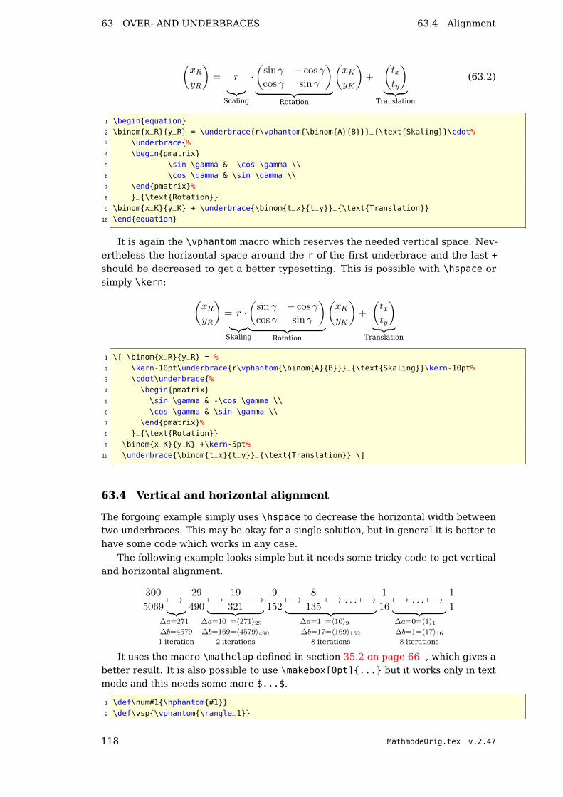
63 OVER- AND UNDERBRACES 63.4 Alignment

(xRyR

)= r

︸︷︷︸Scaling

·(

sin γ − cos γ

cos γ sin γ

)

︸︷︷︸Rotation

(xKyK

)+

(txty

)

︸︷︷︸Translation

(63.2)

1 \beginequation2 \binomx_Ry_R = \underbracer\vphantom\binomAB_\textSkaling\cdot%3 \underbrace%4 \beginpmatrix5 \sin \gamma & -\cos \gamma \\6 \cos \gamma & \sin \gamma \\7 \endpmatrix%8 _\textRotation9 \binomx_Ky_K + \underbrace\binomt_xt_y_\textTranslation

10 \endequation

It is again the \vphantom macro which reserves the needed vertical space. Nev-ertheless the horizontal space around the r of the first underbrace and the last +should be decreased to get a better typesetting. This is possible with \hspace orsimply \kern:

(xRyR

)= r

︸︷︷︸Skaling

·(

sin γ − cos γ

cos γ sin γ

)

︸︷︷︸Rotation

(xKyK

)+

(txty

)

︸︷︷︸Translation

1 \[ \binomx_Ry_R = %2 \kern-10pt\underbracer\vphantom\binomAB_\textSkaling\kern-10pt%3 \cdot\underbrace%4 \beginpmatrix5 \sin \gamma & -\cos \gamma \\6 \cos \gamma & \sin \gamma \\7 \endpmatrix%8 _\textRotation9 \binomx_Ky_K +\kern-5pt%

10 \underbrace\binomt_xt_y_\textTranslation \]

63.4 Vertical and horizontal alignment

The forgoing example simply uses \hspace to decrease the horizontal width betweentwo underbraces. This may be okay for a single solution, but in general it is better tohave some code which works in any case.

The following example looks simple but it needs some tricky code to get verticaland horizontal alignment.

300

50697−→︸︷︷︸

∆a=271

∆b=4579

1 iteration

29

4907−→ 19

3217−→

︸︷︷︸∆a=10 =〈271〉29∆b=169=〈4579〉490

2 iterations

9

1527−→ 8

1357−→ . . . 7−→

︸︷︷︸∆a=1 =〈10〉9∆b=17=〈169〉152

8 iterations

1

167−→ . . . 7−→︸︷︷︸∆a=0=〈1〉1∆b=1=〈17〉16

8 iterations

1

1

It uses the macro \mathclap defined in section 35.2 on page 66 , which gives abetter result. It is also possible to use \makebox[0pt]... but it works only in textmode and this needs some more $...$.

1 \def\num#1\hphantom#12 \def\vsp\vphantom\rangle_1


64 INTEGRALS

3

4 \beginequation*5 \frac3005069%6 \underbrace\longmapsto\vphantom\frac11_%7 \mathclap\substack%8 \Delta a=271\num9\vsp \\[2pt]9 \Delta b=4579\vsp\\[2pt]

10 \text$1$ iteration%11 \frac29490%12 \underbrace\longmapsto \frac19321\longmapsto_%13 \mathclap\substack%14 \Delta a=10\num9=\langle271\rangle_29\num20\\[2pt]15 \Delta b=169=\langle4579\rangle_490\\[2pt]16 \text$2$ iterations17 \frac915218 \underbrace\longmapsto \frac8135\longmapsto\dots\longmapsto_%19 \substack%20 \Delta a=1\num7=\langle10\rangle_9\num119\\[2pt]21 \Delta b=17=\langle169\rangle_152\\[2pt]22 \text$8$ iterations23 \frac11624 \underbrace\longmapsto\dots\longmapsto\vphantom\frac8135_%25 \substack%26 \Delta a=0=\langle1\rangle_1\num76 \\[2pt]27 \Delta b=1=\langle17\rangle_16 \\[2pt]28 \text$8$ iterations29 \frac1130 \endequation*

64 Integrals

The first theorem of Green is:˚

G

[u∇2v + (∇u,∇v)

]d3V =

‹

S

u∂v

∂nd2A

The second theorem of Green is:

˚

G

[u∇2v − v∇2u

]d3V =

‹

S

(u∂v

∂n− v ∂u

∂n

)d2A

They are both written with the esint package38, which gives nice integral symbols.The LATEX code for the first equation is:

1 \[2 \underset\mathcalG\quad\iiint\!%3 \left[u\nabla^2v+\left(\nabla u,\nabla v\right)\right]\mathrmd^3V%4 =\underset\mathcalS\quad\oiint u\,\Qvn\,\,\mathrmd^2A5 \]

with the following definition in the preamble for the partial derivation:

1 \def\Q#1#2\frac\partial#1\partial #2

which makes things easier to write.

38See section 64.


65 HORIZONTAL ALIGNMENT

65 Horizontal alignment

65.1 Over more than one page

Sometimes it may be useful to have a vertical alignment over the whole page with amix of formulas and text. Section 37 shows the use of \intertext. There is anothertrick to get all formulas vertical aligned. Let’s have the following formulas distributedover the whole page:

f(x) = a

g(x) = x2 − 4x

f(x)− g(x) = x2 + x3 + x

g(x) = x2 + x3 + x4 + x5 + b

They all have a different length of the left and right side. Now we want to writesome text and other objects between them, but let the alignment untouched. Wechoose the longest left and the longest right side and take them for scaling with the\hphantom command:

\hphantom\mbox$f(x)-g(x)$ & \hphantom\mbox$= x^2+x^3+x^4+x^5+b$

This is the first (empty) line in every equation where now all other lines arealigned to this one. For example:

blah blah blah blah blah blah blah blah blah blah blah blah blah blah blah blah blahblah blah blah blah blah blah blah

f(x) = a (65.1)

g(x) = x2 − 4x (65.2)


f(x)− g(x) = x2 + x3 + x (65.3)


g(x) = x2 + x3 + x4 + x5 + b (65.4)


The phantom line is empty but leaves the vertical space for a line. This could becorrected with decreasing the \abovedisplayshortskip length and done all insidea group.

1 \newcommand\xblah blah blah blah blah blah blah blah 2 \bgroup3 \addtolength\abovedisplayshortskip-0.5cm% decrease the skip


65.2 Special text columns 65 HORIZONTAL ALIGNMENT

4 \addtolength\abovedisplayskip-0.5cm5 \x\x\x6 \beginalign7 \hphantom\mbox$f(x)-g(x)$ & \hphantom\mbox$= x^2+x^3+x^4+x^5+b$\nonumber\\8 f(x) &= a\\9 g(x) &= x^2-4x

10 \endalign11 %12 \x\x\x13 \beginalign14 \hphantom\mbox$f(x)-g(x)$ & \hphantom\mbox$= x^2+x^3+x^4+x^5+b$\nonumber\\15 f(x)-g(x) &= x^2+x^3+x16 \endalign17 \x\x\x18 %19 \beginalign20 \hphantom\mbox$f(x)-g(x)$ & \hphantom\mbox$= x^2+x^3+x^4+x^5+b$\nonumber\\21 g(x) &= x^2+x^3+x^4+x^5+b22 \endalign23 \x\x\x24 \egroup

Another case of aligning equations inside an itemize environment is the followingone. With the \makebox macro one can have the same size on the left side of theequal sign to get a vertical alignment.

• first functionP1 =

∑

a

∈ A

• but another onesin (P1) = blabla

• or perhapsP3 + P2 − P1 = blablub

1 \newsavebox\lW2 \sbox\lW$P_3+P_2-P_1$3

4 \beginitemize5 \item first function \\6 $\displaystyle\makebox[\wd\lW][r]$P_1$=\sum_a \in A$7 \item but another one \\8 $\makebox[\wd\lW][r]$\sin\left(P_1\right)$=blabla$9 \item or perhaps \\

10 $P_3+P_2-P_1=blablub$11 \enditemize

65.2 Special text columns

This one comes from Hartmut Henkel and offers a special form of placing additionaltext between the equation and the equation number. This makes only sense whenyou load the documentclass with the option fleqn. The example places the additionaltext at 0.5\textwidth, changing this value is no problem.


65 HORIZONTAL ALIGNMENT 65.2 Special text columns

text text text text text text text text text text text text text text text text text text text text texttext text text text text text text text text text text text text text text text text text text text texttext text text text text text text text text text text text text text

ε =E · 4 · π · ε0 · a0 ·

(Z

23i + Z

23

Si

)− 12

Zi · ZSi · e2 ·(

1 + mi

mSi

) ; (65.5)

a0 Bohrscher Radius (= 0,53Å)e ElementarladungNsi Anzahl der Siliziumatome

pro Einheitsvolumenm AtomgewichtZ Kernladungszahl

a2 + b2 = c2 (65.6)abc

z = 9 (65.7)

text text text text text text text text text text text text text text text text text text text text texttext text text text text text text text text text text text text text text text text text text text texttext text text text text text text text text text text text text text

This solution works only with AMSmath, without you have to redefine the LATEXmacro, which creates the equation number.

1 \newsavebox\myendhook % for the tabulars2 \def\tagform@#1(\maketag@@@\ignorespaces#1\unskip\@@italiccorr)3 \makebox[0pt][r]% after the equation number4 \makebox[0.4\textwidth][l]\usebox\myendhook%5 %6 \global\sbox\myendhook% clear box content7 8 [ ... ]9 \sbox\myendhook%

10 \beginfootnotesize%11 \begintabular@ll12 $a_0$ & Bohrscher Radius ($\mathrm= 0,53\,\mbox\AA$)\\13 $e$ & Elementarladung\\14 $N_si$ & Anzahl der Siliziumatome\\15 & pro Einheitsvolumen\\16 $m$ & Atomgewicht\\17 $Z$ & Kernladungszahl18 \endtabular19 \endfootnotesize20 %21 \beginequation22 \varepsilon = \fracE \cdot 4 \cdot \pi \cdot \varepsilon_023 \cdot a_0 \cdot \left( Z_i^\frac23 + Z_Si^\frac2324 \right)^-\frac12 Z_i \cdot Z_Si \cdot e2 \cdot \left( 125 + \fracm_im_Si \right)\,;26 \endequation27 %28 \sbox\myendhookabc29 %30 \beginequation a2+b2=c2 \endequation31 %32 \beginequation z = 9 \endequation


65.3 Centered vertical dots 66 NODE CONNECTIONS

65.3 Centered vertical dots

By default the vertical dots of \vdots are aligned to the left of the = symbol and notcentered.

a1 = b1 c1 = d1 (65.8)

a2 = b2 c2 = d2 (65.9)

a... b

...

an = bn cn = dn (65.10)

1 \usepackageamsmath2 ...3

4 \newsavebox\eqbox5 \sbox\eqbox$\null=\null$6 \newcommand\Vdots\makebox[\wd\eqbox]\vdots7

8 \beginalign9 a_1 & = b_1 & c_1 & = d_1 \\

10 a_2 & = b_2 & c_2 & = d_2 \\11 a & \Vdots b & & \Vdots \nonumber \\12 a_n & = b_n & c_n & = d_n13 \endalign

66 Node connections

This is a typical application for PSTricks and it needs the package pst-node anddoesn’t work with pdflatex. Use vlatex, ps4pdf or ps2pdf.

Die Bindungsenergie im Tropfchenmodell setzt sich aus folgenden Teilen zu-sammen:

• dem Oberflachenanteil

• dem Volumenanteil,

E = avA + − afA2/3 + − ac Z(Z−1)

A1/3 + − as (A−2Z)2

A+ Ep (1)

• dem Coulomb-Anteil

• der Symmetrieenergie

• sowie einem Paarbildungsbeitrag.

1 \pssetnodesep=3pt2 \definecolorlilargb0.6,0.2,0.53 \definecolordarkyellowrgb1,0.9,04 Die Bindungsenergie im Tr\"opfchenmodell setzt sich aus


67 SPECIAL PLACEMENT

5 folgenden Teilen zusammen:6 \beginitemize7 \item dem \rnodebOberfl\"achenanteil8 \item dem \rnodeaVolumenanteil,\\[1cm]9 \def\xstrut\vphantom\frac(A)^1(B)^1

10 \beginequation11 E =12 \rnode[t]ae\psframebox*[fillcolor=darkyellow,13 linestyle=none]\xstrut a_vA +14 \rnode[t]be\psframebox*[fillcolor=lightgray,15 linestyle=none]\xstrut -a_fA^2/3 +16 \rnode[t]ce\psframebox*[fillcolor=green,17 linestyle=none]\xstrut -a_c\fracZ(Z-1)A^1/3 +18 \rnode[t]de\psframebox*[fillcolor=cyan,19 linestyle=none]\xstrut -a_s\frac(A-2Z)^2A +20 \rnode[t]ee\psframebox*[fillcolor=yellow,21 linestyle=none]\xstrut E_p22 \endequation\\[0.25cm]23 \item dem \rnodecCoulomb-Anteil24 \item der \rnodedSymmetrieenergie25 \item sowie einem \rnodeePaarbildungsbeitrag.26 \enditemize27 \nccurve[angleA=-90,angleB=90]->aae28 \nccurve[angleB=45]->bbe \nccurve[angleB=-90]->cce29 \nccurve[angleB=-90]->dde \nccurve[angleB=-90]->eee

67 Special placement of displayed equations

67.1 Formulas side by side

Sometimes it may be useful to have numbered formulas side by side like the followingones:

˛Eds = 0 (67.1.a) ∇ ·B = 0 (67.1.b)

a =c

d(67.2.a) b = 1 (67.2.b)

c = 1 (67.3.a)ˆ

2x dx = x2 + C (67.3.b)

And again a default display equation:

F (x) =

ˆ ∞0

1

xdx (67.4)

1 \beginmtabular*2m0.35\linewidthm0.15\linewidth2 \beginalign* \oint E ds=0 \endalign* & \eqnCnt %3 & \beginalign* \nabla\cdot B=0 \endalign* & \eqnCnt[\labelblah]\\4 \beginalign* a =\fraccd \endalign* & \eqnCnt %5 & \beginalign* b = 1 \endalign* & \eqnCnt\\6 \beginalign* c =1 \endalign* & \eqnCnt[\labelblub]7 & \beginalign* \int 2x \,\mathrmdx = x^2+C \endalign* & \eqnCnt8 \endmtabular


67.1 Formulas side by side 67 SPECIAL PLACEMENT

The new environment mtabular has two arguments, one optional and one whichis the same as the one from the tabular environment. With the option long itis possible to have all the formulas in a longtable environment, which allows apagebreak. The new macro \eqnCnt controls the counting of these equations assubequations for one tabular line. This macro can have an optional argument for alabel. At least it counts the equations. If the equation number is not centered to theforegoing equation, then it needs some more horizontal space in the tabular column.

\eqnCnt[<optional label>]

The vertical space is controlled by the length \mtabskip, which is by default-1.25cm and can be modified in the usual way. To define all these macros write intothe preamble:

1 \usepackageamsmath2 \newcountersubequation3 \newlength\mtabskip\mtabskip=-1.25cm4 \newcommand\eqnCnt[1][]%5 \refstepcountersubequation%6 \beginalign#1\endalign%7 \addtocounterequation-18 \def\mtabLonglong9 \makeatletter

10 \newenvironmentmtabular[2][\empty]%11 \def\@xarraycr%12 \stepcounterequation%13 \setcountersubequation0%14 \@ifnextchar[\@argarraycr\@argarraycr[\mtabskip]15 \let\theoldequation\theequation%16 \renewcommand\theequation\theoldequation.\alphsubequation17 \edef\mtabOption#118 \setcountersubequation0%19 \tabcolsep=0pt20 \ifx\mtabOption\mtabLong\longtable#2\else\tabular#2\fi%21 %22 \ifx\mtabOption\mtabLong\endlongtable\else\endtabular\fi%23 \let\theequation\theoldequation%24 \stepcounterequation25 \makeatother

As seen in equation 67.3.a and equation 67.1.b, everything of the table contents isnonsense . . . And the following tabular is defined as a longtable to enable pagebreaks.

˛Eds = 0 (67.5.a) ∇ ·B = 0 (67.5.b)

a =c

d(67.6.a) b = 1 (67.6.b)

c = 1 (67.7.a)ˆ

2x dx = x2 + C (67.7.b)

˛Eds = 0 (67.8.a) ∇ ·B = 0 (67.8.b)

a =c

d(67.9.a) b = 1 (67.9.b)


67 SPECIAL PLACEMENT 67.2 Itemize environment

c = 1 (67.10.a)ˆ

2x dx = x2 + C (67.10.b)

˛Eds = 0 (67.11.a) ∇ ·B = 0 (67.11.b)

a =c

d(67.12.a) b = 1 (67.12.b)

c = 1 (67.13.a)ˆ

2x dx = x2 + C (67.13.b)

˛Eds = 0 (67.14.a) ∇ ·B = 0 (67.14.b)

a =c

d(67.15.a) b = 1 (67.15.b)

c = 1 (67.16.a)ˆ

2x dx = x2 + C (67.16.b)

As seen in equation 67.13.a and equation 67.11.b, everything is nonsense ...

And again a default display equation:

F (x) =

ˆ ∞0

1

xdx (67.17)

1 \beginmtabular[long]*2m0.375\linewidthm0.125\linewidth2 \beginalign* \oint E ds=0 \endalign* & \eqnCnt %3 & \beginalign* \nabla\cdot B=0 \endalign* & \eqnCnt\\4 \beginalign* a =\fraccd \endalign* & \eqnCnt %5 & \beginalign* b = 1 \endalign* & \eqnCnt\\6 \beginalign* c =1 \endalign* & \eqnCnt7 & \beginalign* \int 2x \,\mathrmdx = x^2+C \endalign* & \eqnCnt\\8

9 [ ... ]

67.2 Formulas inside an itemize enviroment

Without any modification it is not possible to get a numbered equation at thesame height as the symbol of the itemize environment. This depends on the\abovedisplayskip. The formula has to be raised up for exactly this length.

1 \def\itemMath#1%2 \raisebox-\abovedisplayshortskip%3 \parbox0.75\linewidth%4 \beginequation#1\endequation5 %6 \beginitemize7 \item \itemMath f = l 8 \item \itemMath g(x) = \int f(x)\,\mathrmdx 9 \enditemize

• f = l (67.18)


68 ROOTS

• g(x) =

ˆf(x) dx (67.19)

68 Roots

There exists no special symbol for roots which are longer than one line. In suchcases the root should be split into two or more one, like

√a · b · c =

√a · √a ·

√b · √c if

possible. If nothing helps one can use \overline for following lines of the root. Thefollowing example uses the multline environment to get only one equation number:

d(P,Q)|Stat.,Dependent =√

[a11(x1 − y1)2 + a22(x2 − y2)2 + . . .+ app(xp − yp)2] +

[2a12(x1 − y1)(x2 − y2) + 2a13(x1 − y1)(x3 − y3)+

. . .+ 2ap−1,p(xp−1 − yp−1)(xp − yp)] (68.1)

1 \beginmultline2 d(P,Q)|_Stat.,Dependent=\\3 \sqrt\left[a_11(x_1-y_1)^2+a_22(x_2-y_2)^2+4 \ldots+a_pp(x_p-y_p)^2\right]+ \\5 \overline\rule0pt2.5ex6 \left[2a_12(x_1-y_1)(x_2-y_2)+2a_137 (x_1-y_1)(x_3-y_3) + \right.\\8 \overline\rule0pt2.5ex9 \left.\ldots +2a_p-1,p(x_p-1-y_p-1)(x_p-y_p)\right]

10 \endmultline

Alternative:

d(P,Q)|Stat.,Dependent =( [a11(x1 − y1)2 + a22(x2 − y2)2 + . . .+ app(xp − yp)2

]+

[2a12(x1 − y1)(x2 − y2) + 2a13(x1 − y1)(x3 − y3)+

. . .+ 2ap−1,p(xp−1 − yp−1)(xp − yp)])1/2

(68.2)

1 \beginmultline2 d(P,Q)|_Stat.,Dependent=\\3 \left\\left[a_11(x_1-y_1)^2+a_22(x_2-y_2)^2+4 \ldots+a_pp(x_p-y_p)^2\right]+\right. \\5 \left[2a_12(x_1-y_1)(x_2-y_2)+2a_136 (x_1-y_1)(x_3-y_3) + \right.\\7 \left.\left.\ldots +2a_p-1,p(x_p-1-y_p-1)(x_p-y_p)\right]\right\^1/28 \endmultline


Part VIII

Lists, bibliography and index


List of Figures

Figure Page1 multline Alignment demo (the fourth row is shifted to the right with

\shoveright) . . . . . . . . . . . . . . . . . . . . . . . . . . . . . . . 552 Demonstration of \multlinegap (default is 0pt) . . . . . . . . . . . 55


List of Tables

Table Page1 Meaning of \mathsurround . . . . . . . . . . . . . . . . . . . . . . . 122 Difference between the default \bigg and the \biggm command . . 253 Use of the different parentheses for the “big” commands . . . . . . 254 Old font style commands . . . . . . . . . . . . . . . . . . . . . . . . . 305 Fonts in math mode . . . . . . . . . . . . . . . . . . . . . . . . . . . . 306 The meaning of the math spaces . . . . . . . . . . . . . . . . . . . . 317 Spaces in math mode . . . . . . . . . . . . . . . . . . . . . . . . . . . 318 Math styles . . . . . . . . . . . . . . . . . . . . . . . . . . . . . . . . 369 Dots in math mode . . . . . . . . . . . . . . . . . . . . . . . . . . . . 3710 Accents in math mode . . . . . . . . . . . . . . . . . . . . . . . . . . 3711 Vectors with package esvect . . . . . . . . . . . . . . . . . . . . . . 3912 The predefined operators of fontmath.ltx . . . . . . . . . . . . . . 4013 The predefined operators of latex.ltx . . . . . . . . . . . . . . . . 4014 The greek letters . . . . . . . . . . . . . . . . . . . . . . . . . . . . . 4215 Comparison between the different align environments . . . . . . . . 4716 Matrix environments . . . . . . . . . . . . . . . . . . . . . . . . . . . 6017 binom commands . . . . . . . . . . . . . . . . . . . . . . . . . . . . . 6218 The modulo commands and their meaning . . . . . . . . . . . . . . . 6419 Different mathcommands . . . . . . . . . . . . . . . . . . . . . . . . 7320 The predefined operators of amsopn.sty . . . . . . . . . . . . . . . . 9121 Predefined math symbols from fontmath.ltx . . . . . . . . . . . . . 10522 New symbols in combination with the equal sign . . . . . . . . . . . 107


References

[1] Paul W. Abrahams, Karl Berry, and Kathryn Hargreaves. TEX for the Impatient.http://tug.org/ftp/tex/impatient/book.pdf, 2003.

[2] Claudio Beccari. Typesetting mathematics for science and technologyaccording to ISO 31/XI. TUGboat, 18(1):39–47, 1997.

[3] Thierry Bouche. Diversity in math fonts. TUGboat, 19(2):121–135, 1998.

[4] David Cobac. Atelier documents mathématiques.http://dcobac.free.fr/spip/IMG/pdf/presentation4.pdf, 2004.

[5] David Cobac. Ecrire des mathématiques avec LATEX.http://dcobac.free.fr/spip/IMG/pdf/prepdocmaths.pdf, 2004.

[6] Michael Downes. Technical notes on the amsmath package. AmericanMathematical Society,ftp://ftp.ams.org/pub/tex/doc/amsmath/technote.pdf, 1999.

[7] Michael Downes. Short Math Guide for LATEX. American Mathematical Society,ftp://ftp.ams.org/pub/tex/doc/amsmath/short-math-guide.pdf, 2002.

[8] Victor Eijkhout. TEX by Topic. http://www.eijkhout.net/tbt/, 1992.

[9] Michel Goossens and Frank Mittelbach. The LATEX Companion. Addison Wesley,2nd edition, 2004.

[10] George Grätzer. Math into LATEX. Birkhäuser Boston, third edition, 2000.

[11] George Grätzer. More Math into LATEX. Springer, 4th edition, 2007.

[12] Donald E. Knuth. The TEXbook. Addison Wesley Professional, 1986. 21stprinting.

[13] Donald E. Knuth, Tracy Larrabee, and Paul M. Roberts. Mathematical Writing.Stanford University, Computer Science Department,http://sunburn.stanford.edu/~knuth/papers/mathwriting.tex.gz, 1987.

[14] R. Kuhn, R. Scott, and L. Andreev. An Introduction to Using TEX in the HarvardMathematics Department. Harvard University, Department of Mathematics,http://abel.math.harvard.edu/computing/latex/manual/texman.html.

[15] Johannes Küster. Designing Math Fonts.http://www.typoma.com/publ/20040430-bachotex.pdf, apr 2004. Vortragauf der polnischen TEX-Konferenz ‘BachoTEX’.

[16] Johannes Küster. Fonts for Mathematics.http://www.typoma.com/publ/20041002-atypi.pdf, oct 2004. Vortrag aufder ATypI-Konferenz in Prag.

[17] Richard Lawrence. Math=Typography? TUGboat, 24(2):165–168, 2003.

[18] NIST. Typefaces for Symbols in Scientific Manuscripts.http://physics.nist.gov/Document/typefaces.pdf, 2004.


http://tug.org/ftp/tex/impatient/book.pdf

http://dcobac.free.fr/spip/IMG/pdf/presentation4.pdf

http://dcobac.free.fr/spip/IMG/pdf/prepdocmaths.pdf

ftp://ftp.ams.org/pub/tex/doc/amsmath/technote.pdf

ftp://ftp.ams.org/pub/tex/doc/amsmath/short-math-guide.pdf

http://www.eijkhout.net/tbt/

http://sunburn.stanford.edu/~knuth/papers/mathwriting.tex.gz

http://abel.math.harvard.edu/computing/latex/manual/texman.html

http://www.typoma.com/publ/20040430-bachotex.pdf

http://www.typoma.com/publ/20041002-atypi.pdf

http://physics.nist.gov/Document/typefaces.pdf

[19] Luca Padovani. MathML formatting with TEX rules and TEX fonts. TUGboat,24(1):53–61, 2003.

[20] Sebastian Rahtz and Leonor Barroca. A style option for rotated objects in LATEX.TUGboat, 13(2):156–180, July 1992.

[21] Steve Seiden. Math cheat sheet. TUG,http://www.tug.org/texshowcase/#math, 2000.

[22] Carole Siegfried and Herbert Voß. Mathematik im Inline-Modus. Die TEXnischeKomödie, 3/04:25–32, November 2004.

[23] Paul Taylor. Commutative Diagrams in TEX. Department of Computer Science,Queen Mary and Westfield College, http://www.paultaylor.eu/diagrams/,2000.

[24] Herbert Voß. Farbige Mathematik. Die TEXnische Komödie, 2/04:81–87, March2004.

[25] Herbert Voß. Mathematiksatz in LATEX. LOB-media.de, Berlin/Heidelberg, 2009.

[26] Herbert Voß. LATEX Referenz. LOB-media.de, Berlin, Heidelberg, 2. edition,2010.

[27] Herbert Voß. Typesetting Mathematics with LATEX. UIT, Cambridge, 2010.


http://www.tug.org/texshowcase/#math

http://www.paultaylor.eu/diagrams/

Index

Symbols$, 9–11\!, 100$, 9$, 9\„ 31\:, 31\;, 31\[, 12, 34\], 12, 34

A\above, 84\abovedisplayshortskip, 33\abovedisplayshortskip, 75\abovedisplayskip, 33\abovedisplayskip, 34, 75, 126\abovewithdelims, 84\acute, 37\acute, 37alignat, 53aligned, 53Alignment– left, 50\allowdisplaybreaks, 42\ArcCos, 94\ArcCot, 94\ArcCsc, 94\ArcSec, 94\ArcSin, 94\ArcTan, 94array, 52array, 20, 34, 91, 92\arraycolsep, 17, 19\arraystretch, 34Arrows, 70\atop, 66\atop, 22, 43, 85\atopwithdelims, 85

B\bar, 37\bar, 37\belowdisplayshortskip, 33\belowdisplayshortskip, 75\belowdisplayskip, 33\belowdisplayskip, 34, 75

\bf, 30\Big, 24\big, 24Bigg, 27\Bigg, 24\bigg, 24\Biggm, 25\biggm, 25\Bigl, 24\bigl, 24\Bigm, 25\bigm, 25\bigr, 24Binom, 43\Binomial, 95\binoppenalty, 88\Bmatrix, 60\bmatrix, 60Bold greek letters, 72\boldmath, 43\boldmath, 44\boldsymbol, 72\bordermatrix, 20\bordermatrix, 20\boxed, 72boxed inline math, 11Braces, 93– Problems, 67\Braket, 93\breve, 37\breve, 37

C\cal, 30\cancel, 94Cases– numbered lines, 110\cases, 18, 59\catcode, 79\cdot, 108\cdots, 37\cdots, 108centertags, 46\cfrac, 61\chapter, 10\check, 37\check, 37

133

\choose, 43

\clap, 67

cmex10, 28

cmr, 102

colon, 108

Color, 43

color, 115

\colorbox, 11

\columncolor, 115

comma, 32, 108

Computer modern, 102

\cong, 107

\Cos, 94

\Cot, 94

\Csc, 94

ctagsplit, 66

D\DblFactorial, 95

\ddddot, 60

\dddot, 37, 60

\dddot, 37

\ddot, 37

\ddot, 37

\ddots, 37

decimal point, 32

\DeclareMathDelimiter, 79

\delcode, 79

Delimiter, 12, 28

\delimiter, 79

\delimiterfactor, 28, 75

\delimitershortfall, 28, 76

description, 44

\dfrac, 62

\dfrac, 10

differential equation, 108

Display math mode, 9

\displaybreak, 42

displayindent, 77

\displayindent, 76

\displaylimits, 85

displaymath, 17

\displaystyle, 62

\displaystyle, 10, 36, 80, 81

\displaywidowpenalty, 89

\displaywidth, 77

dot, 32, 108

\dot, 37

\dot, 37

\doteq, 107\dotsb, 37\dotsc, 37\dotsi, 37\dotsm, 37\dotso, 37double stroke, 30dsfont, 30

Eellipses, 108empheq, 97\ensuremath, 42Environment– array, 20, 34, 91, 92– description, 44– displaymath, 17– empheq, 97– eqnarray, 13, 17, 34, 47, 96– equation, 17, 34– gathered, 100– graphicx, 100– lgathered, 99– matrix, 22– tabular, 18\eqdef, 42eqnarray, 13, 17, 34, 47, 96\eqno, 85Equation– number, 66– numbering, 64equation, 17, 34Equation number, 65equation number, 121\equiv, 107\everydisplay, 45\everydisplay, 86\everymath, 45\everymath, 86Exponent, 39Extensible arrows, 70

F\Factorial, 95\fam, 80\fbox, 11, 16, 97\fboxrule, 11\fboxsep, 11fleqn, 46fleqn, 34


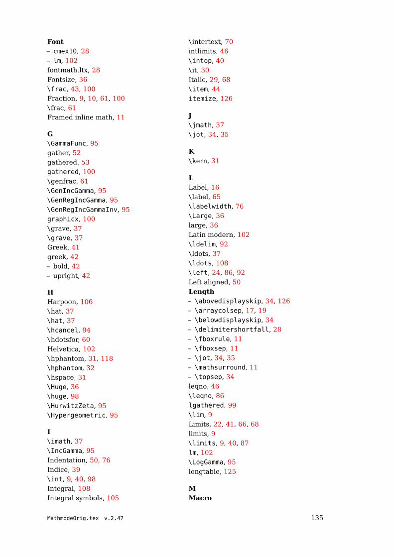
Font– cmex10, 28– lm, 102fontmath.ltx, 28Fontsize, 36\frac, 43, 100Fraction, 9, 10, 61, 100\frac, 61Framed inline math, 11

G\GammaFunc, 95gather, 52gathered, 53gathered, 100\genfrac, 61\GenIncGamma, 95\GenRegIncGamma, 95\GenRegIncGammaInv, 95graphicx, 100\grave, 37\grave, 37Greek, 41greek, 42– bold, 42– upright, 42

HHarpoon, 106\hat, 37\hat, 37\hcancel, 94\hdotsfor, 60Helvetica, 102\hphantom, 31, 118\hphantom, 32\hspace, 31\Huge, 36\huge, 98\HurwitzZeta, 95\Hypergeometric, 95

I\imath, 37\IncGamma, 95Indentation, 50, 76Indice, 39\int, 9, 40, 98Integral, 108Integral symbols, 105

\intertext, 70

intlimits, 46

\intop, 40

\it, 30

Italic, 29, 68

\item, 44

itemize, 126

J\jmath, 37

\jot, 34, 35

K\kern, 31

LLabel, 16

\label, 65

\labelwidth, 76

\Large, 36

large, 36

Latin modern, 102

\ldelim, 92

\ldots, 37

\ldots, 108

\left, 24, 86, 92

Left aligned, 50

Length– \abovedisplayskip, 34, 126

– \arraycolsep, 17, 19

– \belowdisplayskip, 34

– \delimitershortfall, 28

– \fboxrule, 11

– \fboxsep, 11

– \jot, 34, 35

– \mathsurround, 11

– \topsep, 34

leqno, 46

\leqno, 86

lgathered, 99

\lim, 9

Limits, 22, 41, 66, 68

limits, 9

\limits, 9, 40, 87

lm, 102

\LogGamma, 95

longtable, 125

MMacro


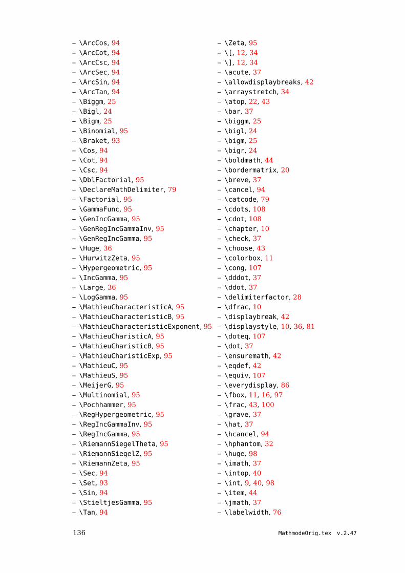
– \ArcCos, 94

– \ArcCot, 94

– \ArcCsc, 94

– \ArcSec, 94

– \ArcSin, 94

– \ArcTan, 94

– \Biggm, 25

– \Bigl, 24

– \Bigm, 25

– \Binomial, 95

– \Braket, 93

– \Cos, 94

– \Cot, 94

– \Csc, 94

– \DblFactorial, 95

– \DeclareMathDelimiter, 79

– \Factorial, 95

– \GammaFunc, 95

– \GenIncGamma, 95

– \GenRegIncGammaInv, 95

– \GenRegIncGamma, 95

– \Huge, 36

– \HurwitzZeta, 95

– \Hypergeometric, 95

– \IncGamma, 95

– \Large, 36

– \LogGamma, 95

– \MathieuCharacteristicA, 95

– \MathieuCharacteristicB, 95

– \MathieuCharacteristicExponent, 95

– \MathieuCharisticA, 95

– \MathieuCharisticB, 95

– \MathieuCharisticExp, 95

– \MathieuC, 95

– \MathieuS, 95

– \MeijerG, 95

– \Multinomial, 95

– \Pochhammer, 95

– \RegHypergeometric, 95

– \RegIncGammaInv, 95

– \RegIncGamma, 95

– \RiemannSiegelTheta, 95

– \RiemannSiegelZ, 95

– \RiemannZeta, 95

– \Sec, 94

– \Set, 93

– \Sin, 94

– \StieltjesGamma, 95

– \Tan, 94

– \Zeta, 95

– \[, 12, 34

– \], 12, 34

– \acute, 37

– \allowdisplaybreaks, 42

– \arraystretch, 34

– \atop, 22, 43

– \bar, 37

– \biggm, 25

– \bigl, 24

– \bigm, 25

– \bigr, 24

– \boldmath, 44

– \bordermatrix, 20

– \breve, 37

– \cancel, 94

– \catcode, 79

– \cdots, 108

– \cdot, 108

– \chapter, 10

– \check, 37

– \choose, 43

– \colorbox, 11

– \cong, 107

– \dddot, 37

– \ddot, 37

– \delimiterfactor, 28

– \dfrac, 10

– \displaybreak, 42

– \displaystyle, 10, 36, 81

– \doteq, 107

– \dot, 37

– \ensuremath, 42

– \eqdef, 42

– \equiv, 107

– \everydisplay, 86

– \fbox, 11, 16, 97

– \frac, 43, 100

– \grave, 37

– \hat, 37

– \hcancel, 94

– \hphantom, 32

– \huge, 98

– \imath, 37

– \intop, 40

– \int, 9, 40, 98

– \item, 44

– \jmath, 37

– \labelwidth, 76


– \ldelim, 92

– \ldots, 108

– \left, 24, 92

– \limits, 9, 40, 87

– \lim, 9

– \makebox, 23, 121

– \mathbf, 44, 92

– \mathchar, 81

– \mathcode, 79

– \mathlarger, 100

– \mathord, 33

– \mathpunct, 33

– \mathring, 37

– \mathrlap, 107

– \mathversion, 44

– \mbox, 29

– \medmuskip, 31, 32

– \nicefrac, 100

– \nolimits, 40

– \nonumber, 12–14

– \ointop, 40

– \oint, 40

– \overbrace, 37, 39

– \overbracket, 37

– \overleftarrow, 37

– \overleftrightarrow, 37

– \overline, 37

– \overrightarrow, 37

– \overset, 23

– \parbox, 29

– \part, 10

– \pmb, 41

– \prod, 9, 22

– \rdelim, 92

– \right, 24, 92

– \scalebox, 100

– \scriptscriptstyle, 36, 81

– \scriptstyle, 36, 81

– \section, 10, 44

– \show, 32

– \smash, 24

– \sqrt, 23

– \stackrel, 42

– \sum, 9, 22, 98

– \texorpdfstring, 10

– \textstyle, 29, 36, 81

– \thickmuskip, 31

– \thinmuskip, 31, 32

– \tilde, 37

– \underbar, 37

– \underbrace, 37, 38

– \underbracket, 37

– \underleftarrow, 37

– \underleftrightarrow, 37

– \underline, 37

– \underrightarrow, 37

– \underset, 23

– \vec, 37

– \vert, 28

– \vphantom, 23, 93

– \vskip, 35

– \widehat, 37

– \widetilde, 37

– \xymatrix, 101

\makebox, 23, 121

\mapstofill, 71

Math operator, 9

Math unit, 63

math unit, 30

\mathaccent, 80

\mathbb, 30

\mathbf, 30

\mathbf, 44, 92

\mathbin, 81

\mathcal, 30

\mathchar, 81

\mathchardef, 81

\mathchoice, 81

\mathclap, 67, 118

\mathclose, 82

\mathcode, 79, 82

\mathds, 30

\mathfrak, 30

Mathieu

– Characteristics, 95

– Functions, 95

\MathieuC, 95

\MathieuCharacteristicA, 95

\MathieuCharacteristicB, 95

\MathieuCharacteristicExponent, 95

\MathieuCharisticA, 95

\MathieuCharisticB, 95

\MathieuCharisticExp, 95

\MathieuS, 95

\mathindent, 46

\mathinner, 87

\mathit, 30

\mathlarger, 100


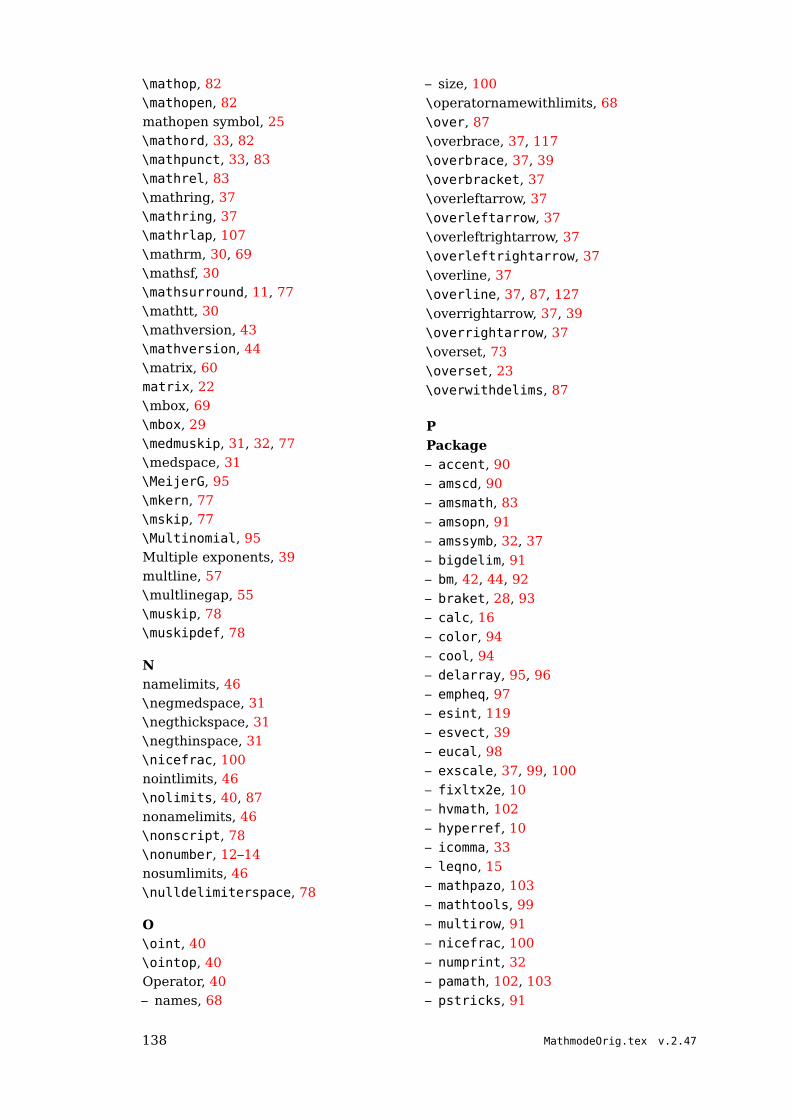
\mathop, 82\mathopen, 82mathopen symbol, 25\mathord, 33, 82\mathpunct, 33, 83\mathrel, 83\mathring, 37\mathring, 37\mathrlap, 107\mathrm, 30, 69\mathsf, 30\mathsurround, 11, 77\mathtt, 30\mathversion, 43\mathversion, 44\matrix, 60matrix, 22\mbox, 69\mbox, 29\medmuskip, 31, 32, 77\medspace, 31\MeijerG, 95\mkern, 77\mskip, 77\Multinomial, 95Multiple exponents, 39multline, 57\multlinegap, 55\muskip, 78\muskipdef, 78

Nnamelimits, 46\negmedspace, 31\negthickspace, 31\negthinspace, 31\nicefrac, 100nointlimits, 46\nolimits, 40, 87nonamelimits, 46\nonscript, 78\nonumber, 12–14nosumlimits, 46\nulldelimiterspace, 78

O\oint, 40\ointop, 40Operator, 40– names, 68

– size, 100

\operatornamewithlimits, 68

\over, 87

\overbrace, 37, 117

\overbrace, 37, 39

\overbracket, 37

\overleftarrow, 37

\overleftarrow, 37

\overleftrightarrow, 37

\overleftrightarrow, 37

\overline, 37

\overline, 37, 87, 127

\overrightarrow, 37, 39

\overrightarrow, 37

\overset, 73

\overset, 23

\overwithdelims, 87

PPackage– accent, 90

– amscd, 90

– amsmath, 83

– amsopn, 91

– amssymb, 32, 37

– bigdelim, 91

– bm, 42, 44, 92

– braket, 28, 93

– calc, 16

– color, 94

– cool, 94

– delarray, 95, 96

– empheq, 97

– esint, 119

– esvect, 39

– eucal, 98

– exscale, 37, 99, 100

– fixltx2e, 10

– hvmath, 102

– hyperref, 10

– icomma, 33

– leqno, 15

– mathpazo, 103

– mathtools, 99

– multirow, 91

– nicefrac, 100

– numprint, 32

– pamath, 102, 103

– pstricks, 91


– relsize, 100– remreset, 14– setspace, 35– units, 100– upgreek, 42– wasysym, 97– xypic, 91, 101– xy, 101Pagebreak, 42Palatino, 102, 103\parbox, 59\parbox, 29\part, 10\phantom, 111\pmatrix, 60\pmb, 72\pmb, 41\Pochhammer, 95Polylogarithm, 95\postdisplaypenalty, 89\predisplaypenalty, 89\predisplaystyle, 78\prod, 9, 22punctuation, 108

Q\qquad, 31\quad, 31

R\radical, 88\rdelim, 92Reference, 16\reflectbox, 37\RegHypergeometric, 95\RegIncGamma, 95\RegIncGammaInv, 95\relpenalty, 89reqno, 46\RiemannSiegelTheta, 95\RiemannSiegelZ, 95\RiemannZeta, 95\right, 24, 88, 92righttag, 66\rm, 30Root, 23, 63, 127\rowcolor, 115

S\scalebox, 100

\scriptfont, 83

\scriptscriptfont, 83

\scriptscriptstyle, 36, 81, 83

\scriptspace, 78

scriptstyle, 9

\scriptstyle, 10, 62

\scriptstyle, 36, 81, 83

\Sec, 94

\section, 10, 44

\Set, 93

Set symbol, 30

\shoveright, 55

\show, 32

\sideset, 68

\Sin, 94

Size

– Operator, 100

\skew, 83

\skewchar, 84

\smallmatrix, 60

\smash, 24

Spacing

– vertical, 35

Split equation, 51

\sqrt, 23

Stacked limits, 67

\stackrel, 42

\StieltjesGamma, 95

Style, 36

Subequations, 64

Subscript, 9

subscript, 22

\substack, 66, 67, 118

\sum, 68

\sum, 9, 22, 98

sumlimits, 46

Superscript, 9

Ttabular, 18

\tag, 16

\Tan, 94

tbtags, 46

\texorpdfstring, 10

Text, 29

– \parbox, 29

\textfont, 84

\textstyle, 29, 36, 81, 84

\tfrac, 62


\thickmuskip, 31, 78\thickspace, 31\thinmuskip, 31, 32, 78\thinspace, 31\tilde, 37\tilde, 37\topsep, 34\tt, 30

U\unboldmath, 43\underbar, 37\underbar, 37\underbrace, 37, 117, 118\underbrace, 37, 38\underbracket, 37\underleftarrow, 37\underleftarrow, 37\underleftrightarrow, 37\underleftrightarrow, 37\underline, 37, 45\underline, 37, 88\underrightarrow, 37\underrightarrow, 37\underset, 73, 119\underset, 23Upright letters, 39upright mode, 22\uproot, 62

V\vcenter, 88\vdots, 37, 123\vec, 37\vec, 37Vector, 39, 113\vert, 28Vertical spacing, 35\Vmatrix, 60\vmatrix, 60\vphantom, 118\vphantom, 23, 93\vskip, 35

W\widehat, 37\widehat, 37\widetilde, 37\widetilde, 37

X

\xleftharpoondown, 106\xleftharpoonup, 106\xleftrightharpoons, 106\xrightharpoondown, 106\xrightharpoonup, 106\xrightleftharpoons, 106\xymatrix, 101

ZZeta, 95– Functions, 95– Hurwitz, 95– Riemann, 95\Zeta, 95


Appendix

A Filelist

This document was build with

1 This is pdfTeXk, Version 3.1415926-1.40.9 (Web2C 7.5.7) (format=pdflatex 2008.10.24) 30 OCT 200810:19

and with the following file and package versions:

1 *File List*2 article.cls 2005/09/16 v1.4f Standard LaTeX document class3 size11.clo 2005/09/16 v1.4f Standard LaTeX file (size option)4 fixltx2e.sty 2006/03/24 v1.1n fixes to LaTeX5 fontenc.sty6 t1enc.def 2005/09/27 v1.99g Standard LaTeX file7 inputenc.sty 2006/05/05 v1.1b Input encoding file8 latin1.def 2006/05/05 v1.1b Input encoding file9 bera.sty 2004/01/31 (WaS)

10 fontenc.sty11 t1enc.def 2005/09/27 v1.99g Standard LaTeX file12 textcomp.sty 2005/09/27 v1.99g Standard LaTeX package13 ts1enc.def 2001/06/05 v3.0e (jk/car/fm) Standard LaTeX file14 beraserif.sty 2004/01/30 (WaS)15 keyval.sty 1999/03/16 v1.13 key=value parser (DPC)16 t1fve.fd 2004/09/07 scalable font definitions for T1/fve.17 berasans.sty 2004/01/30 (WaS)18 beramono.sty 2004/01/31 (WaS)19 ifpdf.sty 2007/12/12 v1.6 Provides the ifpdf switch (HO)20 ifvtex.sty 2007/09/09 v1.3 Switches for detecting VTeX and its modes (HO)21 comment.sty22 graphicx.sty 1999/02/16 v1.0f Enhanced LaTeX Graphics (DPC,SPQR)23 graphics.sty 2006/02/20 v1.0o Standard LaTeX Graphics (DPC,SPQR)24 trig.sty 1999/03/16 v1.09 sin cos tan (DPC)25 graphics.cfg 2007/01/18 v1.5 graphics configuration of teTeX/TeXLive26 pdftex.def 2008/09/08 v0.04l Graphics/color for pdfTeX27 varwidth.sty 2003/03/10 ver 0.9a; Variable-width minipages28 array.sty 2005/08/23 v2.4b Tabular extension package (FMi)29 delarray.sty 1994/03/14 v1.01 array delimiter package (DPC)30 tabularx.sty 1999/01/07 v2.07 ‘tabularx’ package (DPC)31 amsmath.sty 2000/07/18 v2.13 AMS math features32 amstext.sty 2000/06/29 v2.0133 amsgen.sty 1999/11/30 v2.034 amsbsy.sty 1999/11/29 v1.2d35 amsopn.sty 1999/12/14 v2.01 operator names36 amssymb.sty 2002/01/22 v2.2d37 amsfonts.sty 2001/10/25 v2.2f38 bm.sty 2004/02/26 v1.1c Bold Symbol Support (DPC/FMi)39 upgreek.sty 2003/02/12 v2.0 (WaS)40 cancel.sty 2000/03/12 v2.1 Cancel math terms41 amscd.sty 1999/11/29 v1.2d42 accents.sty 2006/05/12 v1.3 Math Accent Tools43 dsfont.sty 1995/08/01 v0.1 Double stroke roman fonts44 multirow.sty45 bigdelim.sty46 framed.sty 2007/10/04 v 0.95: framed or shaded text with page breaks47 longtable.sty 2004/02/01 v4.11 Multi-page Table package (DPC)48 varioref.sty 2006/05/13 v1.4p package for extended references (FMi)49 xcolor.sty 2007/01/21 v2.11 LaTeX color extensions (UK)50 color.cfg 2007/01/18 v1.5 color configuration of teTeX/TeXLive


51 makeidx.sty 2000/03/29 v1.0m Standard LaTeX package52 url.sty 2006/04/12 ver 3.3 Verb mode for urls, etc.53 setspace.sty 2000/12/01 6.7 Contributed and Supported LaTeX2e package54 empheq.sty 2007/12/03 v2.12 Emphasizing equations (MH)55 mhsetup.sty 2007/12/03 v1.2 programming setup (MH)56 mathtools.sty 2008/08/01 v1.06 mathematical typesetting tools (MH)57 calc.sty 2005/08/06 v4.2 Infix arithmetic (KKT,FJ)58 nicefrac.sty 1998/08/04 v0.9b Nice fractions59 ifthen.sty 2001/05/26 v1.1c Standard LaTeX ifthen package (DPC)60 exscale.sty 1997/06/16 v2.1g Standard LaTeX package exscale61 relsize.sty 2003/07/04 ver 3.162 xspace.sty 2006/05/08 v1.12 Space after command names (DPC,MH)63 eucal.sty 2001/10/01 v2.2d Euler Script fonts64 footmisc.sty 2007/06/12 v5.4a a miscellany of footnote facilities65 esint.sty66 esvect.sty67 remreset.sty68 cool.sty 2006/12/29 v1.35 COntent Oriented LaTeX69 coollist.sty 2007/10/06 v1.2 COntent Oriented LaTeX Lists70 coolstr.sty 2007/01/08 v2.1 COntent Oriented LaTeX Strings71 forloop.sty 2006/09/18 v3.0 For Loops for LaTeX72 bbm.sty 1999/03/15 V 1.2 provides fonts for set symbols - TH73 xypic.sty 1999/02/16 Xy-pic version 3.774 xy.sty75 fancyhdr.sty76 showexpl.sty 2007/02/03 v0.3h Typesetting example code (RN)77 listings.sty 2007/02/22 1.4 (Carsten Heinz)78 lstmisc.sty 2007/02/22 1.4 (Carsten Heinz)79 listings.cfg 2007/02/22 1.4 listings configuration80 lstmisc.sty 2007/02/22 1.4 (Carsten Heinz)81 showexpl.cfg 2005/06/30 v0.02 Definitions for the showexpl package (hv)82 lstlang1.sty 2004/09/05 1.3 listings language file83 lstlang2.sty 2004/09/05 1.3 listings language file84 lstlang3.sty 2004/09/05 1.3 listings language file85 lstlang1.sty 2004/09/05 1.3 listings language file86 lstlang2.sty 2004/09/05 1.3 listings language file87 lstlang3.sty 2004/09/05 1.3 listings language file88 lstlang1.sty 2004/09/05 1.3 listings language file89 lstlang2.sty 2004/09/05 1.3 listings language file90 lstlang3.sty 2004/09/05 1.3 listings language file91 lstlang1.sty 2004/09/05 1.3 listings language file92 lstlang2.sty 2004/09/05 1.3 listings language file93 lstlang3.sty 2004/09/05 1.3 listings language file94 lstmisc.sty 2007/02/22 1.4 (Carsten Heinz)95 microtype.sty 2008/06/04 v2.3b Micro-typography with pdfTeX (RS)96 microtype.cfg 2008/06/04 v2.3b microtype main configuration file (RS)97 hyperref.sty 2008/09/29 v6.78l Hypertext links for LaTeX98 ifxetex.sty 2008/09/18 v0.4 Provides ifxetex conditional99 hycolor.sty 2008/09/08 v1.4 Code for color options of hyperref/bookmark (HO100 )101 xcolor-patch.sty 2008/09/08 xcolor patch102 pd1enc.def 2008/09/29 v6.78l Hyperref: PDFDocEncoding definition (HO)103 etexcmds.sty 2007/12/12 v1.2 Prefix for e-TeX command names (HO)104 infwarerr.sty 2007/09/09 v1.2 Providing info/warning/message (HO)105 hyperref.cfg 2002/06/06 v1.2 hyperref configuration of TeXLive106 kvoptions.sty 2007/10/18 v3.0 Keyval support for LaTeX options (HO)107 bitset.sty 2007/09/28 v1.0 Data type bit set (HO)108 intcalc.sty 2007/09/27 v1.1 Expandable integer calculations (HO)109 bigintcalc.sty 2007/11/11 v1.1 Expandable big integer calculations (HO)110 pdftexcmds.sty 2007/12/12 v0.3 LuaTeX support for pdfTeX utility functions (


111 HO)112 kvsetkeys.sty 2007/09/29 v1.3 Key value parser with default handler support113 (HO)114 atbegshi.sty 2008/07/31 v1.9 At begin shipout hook (HO)115 hpdftex.def 2008/09/29 v6.78l Hyperref driver for pdfTeX116 hypcap.sty 2008/09/08 v1.10 Adjusting anchors of captions (HO)117 babel.sty 2008/07/06 v3.8l The Babel package118 english.ldf 2005/03/30 v3.3o English support from the babel system119 braket.sty120 ts1cmr.fd 1999/05/25 v2.5h Standard LaTeX font definitions121 supp-pdf.tex122 nameref.sty 2007/05/29 v2.31 Cross-referencing by name of section123 refcount.sty 2008/08/11 v3.1 Data extraction from references (HO)124 Mathmode.out125 Mathmode.out126 Mathmode.tex127 mt-cmr.cfg 2008/02/29 v1.9a microtype config. file: Computer Modern Roman128 (RS)129 umsa.fd 2002/01/19 v2.2g AMS font definitions130 mt-msa.cfg 2006/02/04 v1.1 microtype config. file: AMS symbols (a) (RS)131 umsb.fd 2002/01/19 v2.2g AMS font definitions132 mt-msb.cfg 2005/06/01 v1.0 microtype config. file: AMS symbols (b) (RS)133 mt-eur.cfg 2006/07/31 v1.1 microtype config. file: AMS Euler Roman (RS)134 uesint.fd135 uesvect.fd136 ts1fve.fd 2004/09/07 scalable font definitions for TS1/fve.137 t1fvm.fd 2004/09/07 scalable font definitions for T1/fvm.138 images/styles.pdf139 images/amsalign.pdf140 t1fvs.fd 2004/09/07 scalable font definitions for T1/fvs.141 images/family.pdf142 images/EuScript.pdf143 images/exscale.pdf144 images/cm-crop.pdf145 images/lm-crop.pdf146 images/pazo-crop.pdf147 images/pamath-crop.pdf148 images/cmbright-crop.pdf149 images/minionpro-crop.pdf150 images/colArray.pdf151 images/node.pdf152 Mathmode.bbl153 Mathmode.ind
