math 140a: foundations of real analysis itkemp/140a/140a.notes.w2016.pdf · math 140a: foundations...
TRANSCRIPT
MATH 140A: FOUNDATIONS OF REAL ANALYSIS I
TODD KEMP
CONTENTS
1. Ordered Sets, Ordered Fields, and Completeness 11.1. Lecture 1: January 5, 2016 11.2. Lecture 2: January 7, 2016 41.3. Lecture 3: January 11, 2016 71.4. Lecture 4: January 14, 2014 92. Sequences and Limits 132.1. Lecture 5: January 19, 2016 132.2. Lecture 6: January 21, 2016 152.3. Lecture 7: January 26, 2016 182.4. Lecture 8: January 28, 2016 213. Extensions of R: the Extended Real Numbers R and the Complex Numbers C 253.1. Lecture 9: February 2, 2016 253.2. Lecture 10: February 4, 2016 284. Series 324.1. Lecture 11: February 9, 2016 324.2. Lecture 12: February 11, 2016 374.3. Lecture 13: February 16, 2016 425. Metric Spaces 445.1. Lecture 14: February 18, 2016 475.2. Lecture 15: February 23, 2016 505.3. Lecture 16: February 25, 2016 525.4. Lecture 17: February 29, 2016 556. Limits and Continuity 576.1. Lecture 18: March 3, 2016 576.2. Lecture 19: March 8, 2016 606.3. Lecture 20: March 10, 2016 63
1. ORDERED SETS, ORDERED FIELDS, AND COMPLETENESS
1.1. Lecture 1: January 5, 2016.• N, Z, Q, R, C.• R is the “Real numbers”. There is nothing real about them! That is the first, most important
lesson to learn in this class. We will encounter many “obvious” statements that are, in fact,false. We will also see some counterintuitive statements that turn out to be true.
Date: March 9, 2016.1
2 TODD KEMP
• Mathematicians roughly split into two groups: analysts and algebraists. (There’s lots ofoverlap, though.) Roughly speaking, algebraists are largely concerned about equalities,while analysts are largely concerned about inequalities.
Definition 1.1. A total order is a binary relation < on a set S which satisfies:1. transitive: if x, y, z ∈ S, x < y, and y < z, then x < z.2. ordered: given any x, y ∈ S, exactly one of the following is true: x < y, x = y, or y < x.
The usual order relation on Q (and its subsets Z and N) is a total order. As usual, we write x > yto mean y < x, and x ≤ y to mean “x < y or x = y”.
Definition 1.2. Let (S,<) be a totally ordered set. Let E ⊆ S. A lower bound for E is an elementα ∈ S with the property that α ≤ x for each x ∈ E. A upper bound for E is an element β ∈ Swith the property that x ≤ β for each x ∈ E. IfE possesses an upper bound, we sayE is boundedabove; if it possesses a lower bound, it is bounded below.
For example, the set N is bounded below in Z, but it is not bounded above. Any set that has amaximal element is bounded above by its maximum; similarly, any set with a minimal element isbounded below by its minimum.
Definition 1.3. Let (S,<) be a totally ordered set, and let E ⊆ S be bounded above. The leastupper bound or supremum of E, should it exist, is
supE ≡ min{β ∈ S : β is an upper bound of E}.Similarly, if F is bounded below, the greatest lower bound or infimum of F , should it exsit, is
inf F ⊆ S ≡ max{α ∈ S : α is a lower bound of F}.
To work with the definition (of sup, say), we rewrite it slightly. A number σ ∈ S is the supre-mum of E if the following two properties hold:
1. σ is an upper bound of E.2. Given any s ∈ S with s < σ, s is not an upper bound of E; i.e. there exists some x ∈ E
with s < x ≤ σ.
Example 1.4. Consider the set E = { 1n: n ∈ N} ⊂ Q. This set has a maximal element: 1.
So 1 is an upper bound. Moreover, if s ∈ Q is < 1, then s is not an upper bound of E (since1 ∈ E). Thus, 1 = supE. (This argument shows in general that, if E has a maximal element, thenmaxE = supE.)
On the other hand, E has no minimal element. But note that all elements of E are positive, so0 is a lower bound for E. If s is any rational number > 0, there is certainly some n ∈ N with0 < 1
n< s (this is the Archimedean property of the rational field). Hence, no such s is a lower
bound for E. This shows that 0 is the greatest lower bound: 0 = inf E.
Example 1.5. It is well known that√2 is not rational: in other words, there is no rational number
p satisfying p2 = 2. You probably saw this proof in high school. Suppose, for a contradiction, thatp2 = 2. Since p is rational, we can write it in lowest terms as p = m/n for m,n ∈ Z. So we havem2
n2 = 2, or m2 = 2n2. Thus m2 is even, which means that m is even (since the square of an oddinteger is odd). So m = 2k for some k ∈ Z, meaning m2 = 4k2, and so 4k2 = 2n2, from whichit follows that n2 = 2k2 is even. As before, this imples that n is even. But then both m and nare divisible by 2, which means they are not relatively prime. This contradicts the assumption thatp = m/n is in lowest terms.
MATH 140A: FOUNDATIONS OF REAL ANALYSIS I 3
A finer analysis of this situation shows that Q has “holes”. Let
A = {r ∈ Q : r > 0, r2 < 2}, and B = {r ∈ Q : r > 0, r2 > 2}.The set A is bounded above: if q ≥ 3
2then q2 ≥ 9
4> 2, meaning that q /∈ A; the contrapositive is
that if q ∈ A then q < 32, so 3
2is an upper bound for A. In fact, take any positive rational number
r; then r2 > 0 is also rational. By the total order relation, exactrly one of the following threestatements is true: r2 < 2, r2 = 2, or r2 > 2. In other words, Q>0 = A t {r ∈ Q : r > 0, r2 =2} tB. We just showed that the middle set is empty, so
Q>0 = A tB.• Every element b ∈ B is an upper bound for A. Indeed, if a ∈ A and b ∈ B, thena2 < 2 < b2 so 0 < b2− a2 = (b− a)(b+ a), and dividing through by the positive numberb + a shows b − a > 0 so a < b. (This also shows that every element a ∈ A is a lowerbound for B.)• On the other hand, if a ∈ A, then a is not an upper bound for A; i.e. given a ∈ A, there
exists a′ ∈ A with a < a′. To see this, we can just take
a′ = a+2− a2
2 + a=
2a+ 2
a+ 2.
Since a ∈ A, we know a2 < 2 so 2 − a2 > 0, and the denominator 2 + a > 2 > 0, soa′ > a. But we also have
2− (a′)2 =2(a+ 2)2 − (2a+ 2)2
(a+ 2)2=
2a2 + 8a+ 8− 4a2 − 8a− 4
(a+ 2)2=
2(2− a2)(a+ 2)2
> 0,
showing that a′ ∈ A, as claimed.Thus, B is equal to the set of upper bounds of A in Q>0, and similarly A is equal to the set of lowerbounds of B in Q>0.
But then we have the following strange situation. The setA of lower bounds ofB has no greatestelement: we just showed that, given any a ∈ A, there is an a′ ∈ A with a′ > a. Hence, B has nogreatest lower bound: inf B does not exist in Q>0. Similarly, supA does not exists in Q>0.
Example 1.5 viscerally demonstrates that there is a “hole” in Q: the fact that r2 = 2 has nosolution in Q forces the ordered set to be disconnected into two pieces, each of which is veryincomplete: not only does each fail to possess a max/min, they also fail to possess a sup/inf.

4 TODD KEMP
1.2. Lecture 2: January 7, 2016. We now set the stage for the formal study of the real numbers:it is the (unique) complete ordered field. To understand these words, we begin with fields.
Definition 1.6. A field is a set F equipped with two binary operations +, · : F × F → F, calledaddition and multiplication, satisfying the following properties.
(1) Commutativity: ∀a, b ∈ F, a+ b = b+ a and a · b = b · a.(2) Associativity: ∀a, b, c ∈ F, (a+ b) + c = a+ (b+ c) and (a · b) · c = a · (b · c).(3) Identity: there exists elements 0, 1 ∈ F s.t. ∀a ∈ F, 0 + a = a = 1 · a.(4) Inverse: for any a ∈ F, there is an element denoted −a ∈ F with the property that
a+ (−a) = 0. For any a ∈ F \ {0}, there is an element denoted a−1 with the property thata · a−1 = 1.
(5) Distributivity: ∀a, b, c ∈ F, a · (b+ c) = (a · b) + (a · c).
Example 1.7. Here are some examples of fields.1. The field Zp = {[0], [1], . . . , [p− 1]} for any prime p, where the + and · are the usual ones
inherited from the + and · on Z (namely [a] + [b] = [a + b] and [a] · [b] = [a · b] – youstudied this field in Math 109). All finite fields have this form.
2. Q is a field.3. Z is not a field: it fails item (4), lacking multiplicative inverses of all elements other than±1.
4. Let Q(t) denote the set of rational functions of a single variable t with coefficients in Q:
Q(t) =
{p(t)
q(t): p(t), q(t) are polynomials with coefficients in Q and q(t) is not identically 0
}.
With the usual addition and multiplication of functions, Q(t) is a field. For example,(p(t)q(t)
)−1= q(t)
p(t), which exists so long as p(t) is not identically 0 – i.e. as long as the
original rational function p(t)q(t)
is not the 0 function.
Fields are the kinds of number systems that behave the way you’ve grown up believing numbersbehave, as summarized in the following lemma.
Lemma 1.8. Let F be a field. The following properties hold.(1) Cancellation: ∀a, b, c ∈ F, if a+ b = a+ c then b = c. If a 6= 0, if a · b = a · c then b = c.(2) Hungry Zero: ∀a ∈ F, 0 · a = 0.(3) No Zero Divisors: ∀a, b ∈ F, if a · b = 0, then either a = 0 or b = 0.(4) Negatives: ∀a, b ∈ F, (−a)b = −(ab), −(−a) = a, and (−a)(−b) = ab.
Proof. We’ll just prove (2), leaving the others to the reader. For any a ∈ F, note that
0 · a+ a = 0 · a+ 1 · a = (0 + 1) · a = 1 · a = a = 0 + a.
Hence, by (1) (cancellation), it follows that 0 · a = 0. �
Example 1.9. As in Example 1.7.1, we can consider Zn for any positive integer n. This satisfiesall of the properties of Definition 1.6 except (4): inverses don’t always exist. For example, if n canbe factored as n = km for two positive integers k,m > 1, then we have two nonzero elements[k], [m] ∈ Zn such that [k] · [m] = [km] = [n] = [0], which contradicts Lemma 1.8(3) – there arezero divisors. So Zn is not a field when n is composite.
Now, we combine fields with ordered sets.
MATH 140A: FOUNDATIONS OF REAL ANALYSIS I 5
Definition 1.10. An ordered field is a field F which is an ordered set (F, <), where the orderrelation also satisfies the following two properties:
(1) ∀a, b, c ∈ F, if a < b then a+ c < b+ c.(2) ∀a, b ∈ F, if a > 0 and b > 0, then a · b > 0.
From here, all the usual properties mixing the order relation and the field operations follow. Forexample:
Lemma 1.11. Let (F, <) be an ordered field. Then(1) ∀a ∈ F, a > 0 iff −a < 0.(2) ∀a ∈ F \ {0}, a2 > 0. In particular, 1 = 12 > 0.(3) ∀a, b ∈ F, if a > 0 and b < 0, then a · b < 0.(4) ∀a ∈ F, if a > 0 then a−1 > 0.
Proof. For (1), simply add −a to both sides of the inequality. Note, by the properties of <, thismeans F is the union of three disjoint subsets: the positive elements a > 0, the negative elementsa < 0, and the zero element a = 0; and the operation of multiplication by −1 interchanges thepositive and negative elements. So, for (2), we note that our given a 6= 0 must be either positive ornegative; if a > 0 then a2 = a · a > 0 by Definition 1.10(2), while if a < 0 then a2 = (−a)2 > 0by the same argument. For (3), we then have a > 0 and −b > 0, so −(ab) = a · (−b) > 0, whichmeans that ab < 0. Finally, for (4), suppose a−1 < 0. then by (3) we would have 1 = a · a−1 < 0;but by (2) we know 1 > 0. This contradiction shows that a−1 > 0. �
Example 1.12. 1. Q is an ordered field, with its usual order: m1
n1< m2
n2iff m1n2 < m2n1. In
fact, this is the unique total order on the set Q which makes Q into an ordered field.2. Zp is not an ordered field for any prime p. For suppose it were; then by Lemma 1.11(2)
we know that [1] > [0]. Then [2] = [1] + [1] > [1] + [0] = [1], and so by transitivity[2] > [0]. Continuing this way by induction, we get to [p − 1] > [0]. But we also have[0] = [1] + [p− 1] > [0] + [p− 1] = [p− 1]. This is a contradiction.
3. Let F be an ordered field. Denote by Fc the following set of 2× 2 matrices over F:
Fc ={[
a −bb a
]: a, b ∈ F
}.
The determinant of such a matrix is a2 + b2. In an ordered field, we know that a2 > 0 ifa 6= 0, and thus we have the usual property that a2 + b2 = 0 iff a = b = 0. It follows thatall nonzero matrices in Fc are invertible: we can easily verify that
(a2 + b2)−1[
a b−b a
] [a −bb a
]=
[1 00 1
].
If we define
I =
[1 00 1
], J =
[0 −11 0
]then Fc = {aI + bJ : a, b ∈ F}. Note that J2 = −I . It is now an easy exercise to showthat Fc is a field, with +, · being given by matrix addition and multiplication, where I is themultiplicative identity and the additive identity is the 2 × 2 zero matrix. (Note: this is notgenerally true if F is not an ordered field. For example, in Z2 we have 12+(−1)2 = 0, andas a result the matrix with a = b = 1 is not invertible in this case.) Fc is the complexificationof F. We will later construct the complex numbers C as C = Rc.

6 TODD KEMP
3.5 If F is any ordered field, then Fc cannot be ordered – there is no order relation that makesFc into an ordered field. This is actually what Problem 4 on HW1 asks you to prove.
Item 2 above noted that the finite fields Zp are not ordered fields. In fact, ordered fields must beinfinite. The next results shows why this is true.
Lemma 1.13. Let (F, <) be an ordered field. Then, for any n ∈ Z \ {0}, n · 1F 6= 0F.
Here n · 1F = 1F + 1F + · · ·+ 1F. Note that this property is not automatic for fields: for example,in Zp, p · [1] = [0].
Proof. First, 1 · 1F = 1F > 0F by Lemma 1.11(2). Proceeding by induction, suppose we’ve shownthat n · 1F 6= 0F. Then (n + 1) · 1F = n · 1F + 1F > 0 + 1F = 1F > 0F. Thus, for every n > 0,n · 1F > 0F, meaning it is 6= 0. If, on the other hand, n < 0 in Z, then n · 1F = −(−n · 1F) < 0F,so also it is 6= 0F. �
Corollary 1.14. Let F be an ordered field. The map ϕ : Q→ F given by ϕ(mn) = (m·1F)·(n·1F)−1
is an injective ordered field homomorphism.
An ordered field homomorphism is a function which preserves the field operations: ϕ(a + b) =ϕ(a) + ϕ(b), ϕ(a · b) = ϕ(a) · ϕ(b), and ϕ(0) = 0 and ϕ(1) = 1; and preserves the order relation:if a < b then ϕ(a) < ϕ(b). An injective ordered field homomorphism should be thought of as anembedding: we realize Q as a subset of F, in a way that respects all the ordered field structure.
Proof. First we must check that ϕ is well defined: if m1
n1= m2
n2, then m1n2 = m2n1. It then follows
(by an easy induction) that (m1 · 1F) · (n2 · 1F) = (m2 · 1F) · (n1 · 1F). Dividing out on bothsides then shows that (m1 · 1F)(n1 · 1F)−1 = (m2 · 1F) · (n2 · 1F)−1. Thus, ϕ is well-defined. It issimilar and routine to verify that it is an ordered field homomorphism. Finally, to show it is one-to-one, suppose that ϕ(q1) = ϕ(q2) for q1, q2 ∈ Q. Using the homomorphism property, this meansϕ(q1−q2) = ϕ(q1)−ϕ(q2) = 0. Let q1−q2 = m
n; thus, we have ϕ(m
n) = (m ·1F) · (n ·1F)−1 = 0F.
But then, multiplying through by the non-zero (by Lemma 1.13) element n·1F, we havem·1F = 0F,and again by Lemma 1.13, it follows that m = 0. but this means q1 − q2 = m
n= 0, so q1 = q2.
Thus, ϕ is injective. �
Thus, we will from now on think if Q as a subset of any ordered field.
In Lecture 1, we saw that Q “has holes”. In example 1.5, we found two subsets A,B ⊂ Q withthe property that B = the set of upper bounds of A, A = the set of lower bounds of B, and A hasno maximal element, while B has no minimal element. Thus, supA and inf B do not exist. Thisturns out to be a serious obstacle to doing the kind of analysis we’re used to in calculus, so we’dlike to fill in these holes. This motivates our next definition.
MATH 140A: FOUNDATIONS OF REAL ANALYSIS I 7
1.3. Lecture 3: January 11, 2016.
Definition 1.15. An ordered set (S,<) is called complete if every nonempty subset ∅ 6= E ⊆ Sthat is bounded above possesses a supremum supE ∈ S. We also denote this by saying that (S,<)has the least upper bound property.
We could also formulate things in terms of inf, with the greatest lower bound property. Example1.5 demonstrates how these two are typically related. In fact, they are equivalent.
Proposition 1.16. An ordered set (S,<) has the least upper bound property if and only if, for everynonempty subset ∅ 6= F ⊆ S that is bounded below, inf F ∈ S exists.
Proof. We will argue the forward implication: the least upper bound property implies the greatestlower bound property. The converse is very similar.
Let F 6= ∅ be bounded below; then L ≡ {lower bounds for F} is a nonempty subset of S. Ifx ∈ L and y ∈ F , then x ≤ y, which shows that every y ∈ F is an upper bound for L. Thus, L isbounded above and nonempty; by the least upper bound property of S, σ = supL ∈ S exists. Bydefinition of supremum, if x < σ then x is not an upper bound for L; since every element of F isan upper bound for L, this means that such x is not in F . Taking contrapositives, this says that ifz ∈ F then x ≥ σ. So σ is a lower bound for F – i.e. σ ∈ L. This shows that σ = maxL: i.e. σ isthe greatest lower bound of F : σ = inf F . So inf F exists, as claimed. �
Let us now prove some important properties that complete ordered fields possess – propertiesthat are critical for doing all of analysis.
Theorem 1.17. Let F be a complete ordered field.(1) (Archimedean) Let x, y ∈ F with x > 0. Then there exists n ∈ N so that nx > y.(2) (Density of Q) Let x, y ∈ F, with x < y. Then there exists r ∈ Q so that x < r < y.
A field with property (1) is called Archimedean. It tells us (by setting x = 1) that the set N isnot bounded above in the field: there is no y ∈ F that is ≥ every integer. It also tells us (by settingy = 1) that there are no “infinitesimals” – that is, no matter how small a positive number x is, thereis always a positive integer n such that 0 < 1
n< x. This is an absolutely crucial property for a field
to have if we want to talk about limits. And it does not hold in every ordered field.
Example 1.18. In the field Q(t) of rational functions with rational coefficients, it is always possibleto uniquely express a function f(t) ∈ Q(t) in the form f(t) = λ · p(t)
q(t)where λ ∈ Q and p(t), q(t)
are monic polynomials: their highest order terms have coefficient 1. This allows us to define anorder on Q(t): say f(t) < g(t) iff g(t) − f(t) = λp(t)
q(t)where p(t), q(t) are monic and λ > 0.
(This is the same as insisting that the leading coefficients of the numerator and denominator off(t) − g(t) have the same sign.) For example t2−25t+7
t4−1023 > 0 while −t2−25t+7t4−1023 < 0. Then it is easy
but laborious to check that this makes Q(t) into an ordered field. Note: t − n = 1 · t−n1
> 0for any integer n; this means that, in the ordered field Q(t), the element t is greater than everyinteger. I.e. the set Z ⊂ Q(t) actually has an upper bound (e.g. t) in Q(t). This means Q(t) is anon-Archimedean field. In particular, by Theorem 1.17, Q(t) is not a complete ordered field.
Proof of Theorem 1.17. (1) Suppose, for a contradiction, there there is no such n: that is, nx ≤ yfor every n ∈ N. LetE = {nx : n ∈ N}. Then our assumption is that y is an upper bound forE, soE is bounded above. It is also non-empty (it contains x, for example). Thus, since F is complete,it follows that α = supE exists. In particular, since α − x < α, this means that α − x is not an

8 TODD KEMP
upper bound for E, so there is some element e ∈ E with α− x < e. There is some integer m ∈ Nso that e = mx, so we have α − x < mx. But then α < (m + 1)x, and (m + 1)x ∈ E. Thiscontradicts α = supE being an upper bound. This contradiction proves the claim.
(2) Since y − x > 0, by (1) there is an n ∈ N so that n(y − x) > 1. Now, letting y = ±nx andapplying (1) again, we can find two positive integersm1,m2 ∈ N so thatm1 > nx andm2 > −nx;in other words
−m2 < nx < m1.
This shows that the set {k ∈ Z : nx < k ≤ m1} is finite: it is contained in the finite set {−m2 +1,−m2 +2, . . . ,m1}. So, let m = min{k ∈ Z : nx < k}. Then since m− 1 ∈ Z and m− 1 < m,we must have m− 1 ≤ nx.
Thus, we have two inequalities:
n(y − x) > 1, m− 1 ≤ nx < m.
Combining these gives usnx < m ≤ nx+ 1 < ny.
Dividing through by (the positive) n shows that x < mn< y, so setting r = m
ncompletes the
proof. �
Here is another extremely important property that holds in ordered fields; this is crucial for doingcalculus.
Proposition 1.19. Let F be a complete ordered field. For each n ∈ N, let an, bn ∈ F satisfy
a1 ≤ a2 ≤ · · · ≤ an ≤ · · · ≤ bn ≤ · · · ≤ b2 ≤ b1.
Further, suppose that bn − an < 1n
. Then⋂n∈N[an, bn] is nonempty, and consists of exactly one
point.
This is sometimes called the nested intervals property. It is actually equivalent to the least upperbound property. On HW2, you will prove the converse.
Proof. By construction, b1 is an upper bound for {an : n ∈ N}, which is a nonempty set. Thus,by completeness, α = sup an exists in F. Since α is an upper bound for {an}, we have an ≤ αfor every n. On the other hand, since bm ≥ an for every m,n, bm is an upper bound for {an}, andsince α is the least upper bound, it follows that α ≤ bm as well. Thus α ∈ [an, bn] for every n, andso it is in the intersection.
Now, suppose β ∈⋂n[an, bn]. Then either α < β, α > β, or α = β. Suppose, for the moment,
that α < β. Then we have an ≤ α < β ≤ bn for every n, and since bn − an <1n
, it followsthat 0 < β − α < 1
nfor every n. But this violates the Archimedean property of F. A similar
contradiction arises if we assume α > β. Thus α = β, and so α is the unique element of theintersection. �
Note: in the setup of the lemma, it is similar to see that the intersection consists of infn bn; sosupn an = infn bn.
MATH 140A: FOUNDATIONS OF REAL ANALYSIS I 9
1.4. Lecture 4: January 14, 2014. We have now seen several properties possessed by completeordered fields. We would hope to find some examples as well. Here comes the big punchline.
Theorem 1.20. There exists exactly one complete ordered field. We call this field R, the Realnumbers.
We will talk about the proof of Theorem 1.20 as we proceed in the course. The textbook relegatesan existence proof to the end of Chapter 1, through Dedekind cuts. This is an old-fashioned proof,and not very intuitive. We are not going to discuss it presently. Once we have developed a littlemore technology, we will prove the existence claim of the theorem using Cauchy’s construction ofR (through sequences).
We can, however, prove the uniqueness claim. To be precise, here is what uniqueness meansin this case: suppose F and G are two complete ordered fields. Then there exists an ordered fieldisomorphism ϕ : F→ G. That means ϕ is an ordered field homomorphism that is also a bijection.So, from the point of view of ordered fields, F and G are indistinguishable.
The first question is: given two complete ordered fields F and G, how do we define ϕ : F→ G?By Corollary 1.14, Q embeds in each of F and G via Q · 1F and Q · 1G. So we can define ϕ as apartial function by its action on Q:
ϕ(r1F) = r1G, r ∈ Q.The question is: how should we define ϕ on elements of F that are not necessarily in Q · 1F? Well,let x ∈ F \Q. By Theorem 1.17(2), there are rationals an, bn ∈ Q such that
x− 1
2n1F < an1F < x < bn1F < x+
1
2n1F.
In particular, bn − an < 1n
. We should do this carefully and also make sure that a1 ≤ a2 ≤· · · ≤ b2 ≤ b1 – this can be achieved by choosing the an and bn successively, increasing the anor decreasing the bn each step as needed. It follows from Proposition 1.19 that
⋂n[an1G, bn1G]
contains exactly one point, α = supn(an1G) = infn(bn1G). So we define
ϕ(x) = α.
Note: if x ∈ Q, then x · 1G is the unique element in the intersection, meaning that we can take theabove nested intervals definition as the formula for ϕ on all of F, not just the irrational elements.This will be our starting point.
Theorem 1.21. If F and G are two complete ordered fields, then there exists an ordered fieldisomorphism ϕ : F→ G.
Proof. Following our outline from above, we define ϕ as follows. To begin, using the densenessof Q in F, select a1, b1 ∈ Q so that
x− 1
21F < a11F < x < b11F < x+
1
21F.
Now proceed inductively: once we’ve constructed a1, . . . , an−1 and b1, . . . , bn−1, choose an and bnso that
max
{x− 1
2n1F, an−1
}< an1F < x < bn1F < min
{x+
1
2n1F, bn−1
}. (1.1)
Then we have a1 < a2 < · · · < an < · · · < bn < · · · < b2 < b1, and also
bn − an <(x+
1
2n1F
)−(x− 1
2n1F
)=
1
n.
10 TODD KEMP
So by the nested intervals property Proposition 1.19 applied in the field G, we have⋂n∈N
[an1G, bn1G] = {α}
where α = supn an1G = infn bn1G. We thus define ϕ(x) = α.Now we must verify that:• ϕ is well-defined: if a′n, b
′n are some other rational elements satisfying (1.1) then supn an1G =
supn a′n1G. In fact, this follows because we also then have the mixed inequalities
x− 1
2n1F < a′n1F < x < bn1F < x+
1
2n1F
and, as above, we have supn a′n1G = infn bn1G = supn an1G.
• ϕ is an ordered field homomorphism. This is laborious. Let’s check one of the fieldhomomorphism properties: preservation of addition. Let x, y ∈ F, and let an < x < bnand cn < y < dn where bn − an < 1
2n< 1
nand dn − cn < 1
2n< 1
n. Then ϕ(x) = supn an
and ϕ(y) = supn cn. Now, on the other hand, we have
an+cn < x+y < bn+dn, and (bn+dn)−(an+cn) = (bn−an)+(dn−cn) <1
2n+
1
2n=
1
n.
It follows that ϕ(x+y) = sup(an+ cn). So, to see that ϕ(x+y) = ϕ(x)+ϕ(y), it sufficesto show that
if an ↑ & cn ↑ then supn(an + cn) = sup
nan + sup
ncn.
This is also on HW2. The other ordered field homomorphism properties are verified simi-larly.• ϕ is a bijection. First, suppose that x 6= y ∈ F. Then either x < y or x > y; wlog x < y.
Since ϕ is an ordered field homomorphism, it follows that ϕ(x) < ϕ(y). In particular,ϕ(x) 6= ϕ(y). A similar argument in the case x > y shows that ϕ is one-to-one.
Now, fix y ∈ G. For each n, choose an, bn ∈ Q nested so that bn − an < 1n
andan1G < y < bn1G. Mirroring the above arguments, we know that a = supn an1F ∈⋂n[an1F, bn1F]. Since an1F < a < bn1F, we have an1G = ϕ(an1F) < ϕ(a) < ϕ(bn1F) =
bn1G. Thus ϕ(a) ∈⋂n[an1G, bn1G], and this intersection consists of the singleton element
y, by Proposition 1.19. Hence, ϕ(a) = y, and so ϕ is onto.�
So, we see that there can be only one complete ordered field. (They’re like Highlanders.) Apriori, that doesn’t preclude the possibility that there aren’t any at all. To prove that R exists, weneed to first start talking about convergence properties of sequences. That will be our next task.
Before proceeding, let’s return to our motivation for studying sup and inf and introducing com-pleteness: we wanted to fill the “hole” in Q where
√2 should be. To see that we’ve filled at least
that hole, the next result shows that R (the complete ordered field) contains square roots, and infact nth roots, of all positive numbers. First, let’s state some standard results on “absolute value”.
Lemma 1.22. Let F be an ordered field. For x ∈ F, define (as usual)
|x| =
{x, if x ≥ 0
−x, if x < 0.
Then we have the following properties.
MATH 140A: FOUNDATIONS OF REAL ANALYSIS I 11
(1) For all x ∈ F, |x| ≥ 0, and |x| = 0 iff x = 0.(2) For all x, y ∈ F, |x+ y| ≤ |x|+ |y|.(3) For all x, y ∈ F, |xy| = |x||y|.
All of these properties are straightforward but annoying to prove in cases. We will use theabsolute value frequently in all that follows.
Theorem 1.23. Let n ∈ N, n ≥ 1. For any x ∈ R, x > 0, there is a unique y ∈ R, y > 0, so thatyn = x. We denote it by y = x1/n.
Proof of Theorem 1.23. First, for uniqueness: let y1 6= y2 be two positive real numbers, wlogy1 < y2. Then y21 = y1y1 < y1y2 < y2y2 = y22; continuing by induction, we see that yn1 < yn2 . Thatis: the function y 7→ yn is strictly increasing. In particular, it is one-to-one. It follows that therecan be at most one y with yn = x.
Now for existence. Let E = {y ∈ R : y > 0, yn < x}.• E 6= ∅: note that t = x
x+1∈ (0, 1). This means that 0 < tn < t, and so since x
x+1< x, we
have 0 < tn < x, meaning that t ∈ E.• E is bounded above: let s = 1 + x. Then s > 1, and so sn > s > x. Thus, if y ∈ E, thenyn < x < sn, and so 0 < sn− yn = (s− y)(sn−1+ sn−2y+ · · ·+ yn−1). The sum of termsis strictly positive, so we can divide out and find that s− y > 0. Thus s is an upper boundfor E.
Hence, by completeness of R, α = supE exists. Since α is the least upper bound, it follows that,for each k, there is an element yk ∈ E such that yk > α− 1
k. Since ynk < x, we therefore have(
α− 1
k
)n< ynk < x, for all k ∈ N.
But we can expand(α− 1
k
)n=
n∑j=0
(n
j
)αn−j
(−1
k
)−j= αn − 1
k
n∑j=1
(n
j
)αn−j
(−1
k
)j−1.
Thus, we have
αn < x+1
k
n∑j=1
(n
j
)αn−j
(−1
k
)j−1and so, applying the triangle inequality – Lemma 1.22(2) – repeatedly, we have
αn < x+1
k
∣∣∣∣∣n∑j=1
(n
j
)αn−j
(−1
k
)j−1∣∣∣∣∣ ≤ x+1
k·
n∑j=1
(n
j
)αn−k
(1
k
)j−1.
Note that n is fixed, and 1k≤ 1, so for k ≥ 1 we have
(1k
)j−1 ≤ 1. Let M =∑n
k=1
(nj
)αn−k; then
we have
∀k ∈ N αn < x+M
k; i.e. αn − x < M
k.
By the Archimedean property, it follows that αn − x ≤ 0; thus, we have shown that αn ≤ x.On the other hand, let y ∈ E. Then for any k ∈ N we have, by similar calculations,(
y +1
k
)n= yn +
1
k
n∑j=1
(n
k
)yn−j
(1
k
)j−1≤ yn +
1
k·
n∑j=1
(n
j
)yn−j.

12 TODD KEMP
Since y ∈ E, we know yn < x, so ε = x − yn > 0. Let L =∑n
j=1
(nj
)yn−j , which is a positive
constant; by the Archimedean property, there is some k ∈ N so that 1k· L < ε. Thus, for such k,(
y +1
k
)n≤ yn +
L
k< yn + ε = x.
That is: y + 1k∈ E. But y + 1
k> y. That is, for any y ∈ E, there is y′ > y with y ∈ E. So E has
no maximal element. This shows that α /∈ E, and hence αn ≥ x.In conclusion: we’ve shown that αn ≤ x and x ≤ αn. It follows that αn = x. �
On Homework 2, you will flesh out extending this argument to defining xr for x > 0 in R andr ∈ Q, and then extending this further to define xy for x > 0 and y ∈ R. One can use similararguments to define logb(x) for x, b > 0. We will wait a little while until we have a firm groundingin sequences and limits before rigorously developing the calculus of these well-known functions.
MATH 140A: FOUNDATIONS OF REAL ANALYSIS I 13
2. SEQUENCES AND LIMITS
2.1. Lecture 5: January 19, 2016.
Definition 2.1. Let X be a set. A sequence in X is a function a : N → X . Instead of the usualnotation a(n) for the value of the function at n ∈ N, we usually use the notation an = a(n);accordingly, we often refer to the function as (an)n∈N or {an}n∈N, or (when being sloppy) simply(an) or {an}.
In ordered fields, we can talk about limits of sequences. The following definition took half acentury to finalize; its invention (by Weierstraß) is one of the greatest achievements of analysis.
Definition 2.2. Let F be an ordered field, and let (an) be a sequence in F. Let a ∈ F. Say that anconverges to a, written an → a or limn→∞ an = a, if the following holds true:
∀ε > 0 ∃N ∈ N s.t. ∀n ≥ N |an − a| < ε.
Let’s decode the three-quantifier sentence here. What this say is, no matter how small a toleranceε > 0 you want, there is some time N after which all the terms an (for n ≥ N ) are within ε of a.Some convenient language for this is:
Given any ε > 0, we have |an − a| < ε for almost all n.Here we colloquially say that a set S ⊆ N contains almost all positive integers if the complementN \ S is finite. This is equivalent to saying that, after some N , all n ≥ N are in S. So, the limitdefinition is that, for any positive tolerance, no matter how small, almost all of the terms are withinthat tolerance of the limit.
If (an) is a sequence and there exists a so that an → a, we say that (an) converges; if there isno such a, we say that (an) diverges. Here are some examples.
Example 2.3. Consider each of the following sequences in an Archimedean field.(1) an = 1 converges to 1. More generally, if (an) is equal to a constant a for almost all n,
then an → a.(2) an = 1
nconverges to 0.
(3) an = n+ 1n
diverges.(4) an = (−1)n diverges.(5) an = 1 + 1
n(−1)n converges to 1.
(6) an = 4n+17n−4 (defined for n ≥ 1) converges to 4
7.
In all these examples, we proved convergence (when the sequences converged) to a given value.However, a priori, it is not clear whether it might also have been possible to prove convergence toa different value as well. This is not the case: limits are unique.
Lemma 2.4. Let F be an ordered field, and let (an) be a sequence in F. Suppose a, b ∈ F andan → a and an → b. Then a = b.
Proof. Fix ε > 0. We know that there is N1 so that |an − a| < ε2
for all n > N1, and there is N2 sothat |an − b| < ε
2for all n > N2. Thus, for any n > max{N1, N2}, we have
|a− b| = |a− an + an − b| ≤ |a− an|+ |an − b| <ε
2+ε
2= ε.
Now, suppose that a 6= b. Thus a−b 6= 0, which means that |a−b| > 0. So we can take ε = |a−b|above, and we find that |a− b| < |a− b| – a contradiction. Hence, it must be true that a = b. �
14 TODD KEMP
Remark 2.5. Note, in an Archimedean field, we are free to restrict ε = 1k
for some k ∈ N; that is,an equivalent statement of an → a is
Given any k ∈ N, we have |an − a| < 1k
for almost all n.In non-Archimedean fields, this does not suffice. For example, in the field Q(t), to show an(t) →a(t) it does not suffice to show that, for any k ∈ N, |an(t) − a(t)| < 1
kfor all sufficiently large n.
Indeed, what if an(t)− a(t) = 1t? This does not go to 0, but it is < 1
kfor all k ∈ N. Similarly, the
sequence an = 1n
diverges in a non-Archimedean field.
MATH 140A: FOUNDATIONS OF REAL ANALYSIS I 15
2.2. Lecture 6: January 21, 2016.
Proposition 2.6. Let F be a complete ordered field. Let (an) be a sequence in F, and suppose an ↑(i.e. an ≤ an+1 for all n) and bounded above. Let α = sup{an}. Then an → α. Similarly, if bn ↓and bounded below, then β = inf{bn} exists and bn → β.
Proof. Since F is a complete field, α = sup{an} exists in F. Let ε > 0. Then α− ε < α, and so bydefinition there exists some element aN ∈ {an} so that α − ε < aN ≤ α. Now, suppose n ≥ N ;then an ≤ α of course, but also since an ↑ we have an ≥ aN > α − ε. Thus, we have shown that|an − α| = α− an < ε for all n ≥ N , which is to say that an → α.
The decreasing case is similar; alternatively, one can look at an = −bn, which is increasingand bounded above; then we have by the first part that −bn = an → α where α = sup{−bn} =− inf{an} = −β. It follows that bn → −β, using the limit theorems below.
�
In the proposition, we needed (an) to be bounded (above or below); indeed, the sequence an = nis increasing, but not convergent. This is generally true: for any sequence to be convergent, it mustbe bounded (above and below). A sequence that is either increasing or decreasing is called mono-tone. So the proposition shows that monotone sequences either converge, or grow (in absolutevalue) without bound.
This gives us a new perspective on the motivating example that began our discussion of sup andinf. Consider, again, the sets A = {r ∈ Q : r > 0, r2 < 2} and B = {r ∈ Q : r > 0, r2 > 2}. Wesaw that the set of positive rationals is equal to A t B, and therefore supA and inf B do not existin Q. Note that the sequence 1, 1.4, 1.41, 1.414, 1.4142, 1.42431, . . . is in the set A. We recognizethe terms as the decimal approximations to
√2. This sequence looks like it’s going somewhere;
but in fact the only place it can go is stuck in between A and B, which is not in Q. The questionis: why does it look like it’s going somewhere?
Definition 2.7. A sequence (an) in an ordered set is called Cauchy, or is said to be a Cauchysequence, if
∀ε > 0 ∃N ∈ N s.t. ∀n,m ≥ N |an − am| < ε.
That is: a sequence is Cauchy if its terms get and stay close to each other. That is: for any giventolerance ε > 0, there is some time N after which all the terms are within distance ε of aN . Thisnotion is very close to convergence. Indeed:
Lemma 2.8. Any convergent sequence is Cauchy.
Proof. Let (an) be a convergent sequence, with limit a. Fix ε > 0, and choose N large enough sothat |an − a| < ε
2for n > N . Then for any n,m > N ,
|an − am| = |an − a+ a− am| ≤ |an − a|+ |am − a| <ε
2+ε
2= ε.
Hence, (an) is Cauchy. �
But the converse need not be true.
Example 2.9. In Q, the sequence 1, 1.4, 1.41, 1.414, 1.4142, 1.42431, . . . is Cauchy. Indeed, by thedefinition of decimal expansion, if an is the n-decimal expansion of a number, then an+1 and anagree on the first n digits. This means exactly that |am − an| < 1
10nfor any m > n. So, fix ε > 0.
We can certainly find N so that 110N
< ε (since, for example, 110N
< 1N
). Thus, for n,m > N , wehave |an − am| < 1
10min{m,n} <1
10N< ε.
16 TODD KEMP
Here are some more important facts about Cauchy sequences. Note that, by Lemma 2.8, anyfact about Cauchy sequences is also a fact about convergent sequences.
Proposition 2.10. Let (an) be a Cauchy sequences. Then (an) is bounded: there is a constantM > 0 so that |an| ≤M for all n.
Proof. Taking ε = 1, it follows from the definition of Cauchy that there is some N ∈ N so that|an − am| < 1 for all n,m > N . In particular, this shows that |an − aN+1| < 1 for all n > N ,which is to say that aN+1 − 1 < an < aN+1 + 1. Hence |an| < max{|aN+1 − 1|, |aN+1 + 1|}for n > N . So, define M = max{|a1|, . . . , |aN |, |aN+1 − 1|, |aN+1 + 1|}. If n ≤ N, then|an| ≤ M since |an| appears in this list we maximize over; if n > N then, as just shown, |an| <max{|aN+1 − 1|, |aN+1 + 1|} ≤M . The result follows. �
Another useful concept when working with sequences is subsequences.
Definition 2.11. Let {nk : k ∈ N} be a set of positive integers with the property that nk < nk+1
for all k; that is nk is an increasing sequence in N. Let (an) be a sequence. The function k 7→ ank
is called a subsequence of (an), usually denoted (ank).
Example 2.12. (a) Let an = 1n
. Then a2n = 12n
and a2n = 12n
are subsequences. However
bn =
{an if n is oddan/2 if n is even
is not a subsequence of (an). Indeed, bk = ankwhere (nk)∞k=1 = (1, 1, 3, 2, 5, 3, 7, 4, 9, 5, . . .),
and this is not an increasing sequence of integers.(b) Let an = (−1)n. Then a2n = 1 and a2n+1 = −1 are subsequences.
Here is an extremely useful fact about the indices of subsequences: if (nk) is an increasingsequence in N, then nk ≥ k for every k. (This follows by a simple induction.)
Proposition 2.13. Let (an) be a sequence in an ordered set, and (ank) a subsequence.
(1) If (an) is Cauchy, then (ank) is Cauchy.
(2) If (an) is convergent with limit a, then (ank) is convergent with limit a.
(3) If (an) is Cauchy, and (ank) is convergent with limit a, then (an) is convergent with limit a.
Proof. For (1): fix ε > 0 and let N ∈ N be chosen so that |an − am| < ε for n,m > N . Thenwhenever k, ` > N , we have nk ≥ k > N and n` ≥ ` > N , so by definition |ank
− an`| < ε. Thus
(an) is Cauchy. The proof of (2) is very similar. Item (3) is on HW3. �
Before proceeding with the theory of Cauchy sequences, here are some useful facts about con-vergent sequences sequences.
Theorem 2.14. Let (an) and (bn) be convergent sequences in an ordered field F.(1) If an ≤ bn for all sufficiently large n, then limn an ≤ limn bn.(2) (Squeeze Theorem) Suppose also that limn an = limn bn. If (cn) is another sequence, and
an ≤ cn ≤ bn for all sufficiently large n, then (cn) is convergent, and limn cn = limn an =limn bn.
Proof. Let a = limn an and b = limn bn. For (1), fix ε > 0. There is Na ∈ N so that |an − a| < ε2
for n > Na, and there is Nb ∈ N so that |bn−b| < ε2
for n > Nb. Thus, letting N = max{Na, Nb},we have an − a > − ε
2and bn − b < ε
2for n > N . But then
an − bn > a− ε
2− b− ε
2= a− b− ε.
MATH 140A: FOUNDATIONS OF REAL ANALYSIS I 17
Since an ≤ bn for all large n, we therefore have 0 ≥ an − bn > a− b− ε for such n, and thereforea− b− ε < 0. This is true for any ε > 0, and therefore a− b ≤ 0, as claimed.
For (2), we have a = b. Choosing Na, Nb, and N as above, we have − ε2< an − a ≤ cn − a ≤
bn − a < ε2
for all n ≥ N . That is: |cn − a| < ε2< ε for all n ≥ N . This shows cn → a, as
claimed. �
Cauchy sequences give us a way of talking about completeness that is not so wrapped up in theorder properties. As discussed in Example 2.9 last lecture, the “hole” in Q where
√2 should be is
the limit of a sequence in Q which is Cauchy, but does not converge in Q. Instead of filling in theholes by demanding bounded nonempty sets have suprema, we could instead demand that Cauchysequences have limits.
Definition 2.15. Let S be an ordered set. Call S Cauchy complete if every Cauchy sequence in Sactually converges in S.
Q is not Cauchy complete. But, as we will see, R is. In fact, Cauchy completeness is equivalentto the least upper bound property in any Archimedean field. We can prove half of this assertionnow.
18 TODD KEMP
2.3. Lecture 7: January 26, 2016.
Theorem 2.16. Let F be an Archimedean field. If F is Cauchy complete, then F has the nestedintervals property and hence is complete in the sense of Definition 1.15.
Proof. That the nested intervals property implies the least upper bound property is the contentHW2 Exercise 3; so it suffices to verify that F has the nested intervals property. Let (an) and (bn)be sequences in F with an ↑, bn ↓, an ≤ bn, and bn − an < 1
n. Fix ε > 0, and let N ∈ N be large
enough that 1N< ε (here is where the Archimedean property is needed). Thus, for n ≥ N , we have
bn − an < 1n≤ 1
N< ε. Then for m,n > N , wlog m ≥ n, we have
an ≤ am ≤ bn
and so it follows that |an − am| = am − an ≤ bn − an < ε. Thus (an) is a Cauchy sequence. Bythe Cauchy completeness assumption on F, we conclude that a = limn an exists in F.
Now, fix n0, and note that since an ≥ an0 for n ≥ n0, Theorem 2.14(1) shows that a = limn an ≥an0 (thinking of an0 as the limit of the constant sequences (an0 , an0 , . . .)). Similarly, since an ≤ bn0
for all n, it follows that a ≤ bn0 . Thus a ∈⋂n[an, bn], proving this intersection is nonempty. As
usual, it follows that the intersection consists only of {a}. Indeed, if x, y ∈⋂n[an, bn], without
loss of generality label them so that x ≤ y. Thus an ≤ x ≤ y ≤ bn for every n. For given ε > 0,choose n so that bn−an < ε; then y−x < ε. So 0 ≤ y−x < ε for all ε > 0; it follows that x = y.This concludes the proof of the nested intervals property for S. �
Remark 2.17. The use of the Archimedean property is very subtle here. It is tempting to thinkthat we can do without it. This is true if we replace the nested intervals property by a slightlyweaker version: say an ordered S satisfies the weak nested intervals property if, given an ↑, bn ↓,an ≤ bn, and bn − an → 0, then
⋂n[an, bn] contains exactly one point. (This is weaker than the
nested intervals property, because the assumption is stronger: we’re assuming bn − an → 0 here,while in the usual nested intervals property we assume that bn − an < 1
n, which does not imply
bn − an → 0 in the non-Archimedean setting.) The trouble is: this weak nested intervals propertydoes not imply the least upper bound property in the absence of the Archimedean property. Infact, there do exist non-Archimedean fields (which therefore do not have the least upper boundproperty), but are Cauchy complete. (We may explore this a little later.) This is a prime exampleof how counterintuitive analysis can be without the Archimedean property. Soon enough, we willonce-and-for-all demand that it holds true (in the Real numbers), and dispense with these weirdpathologies.
We would like to show the converse is true: that the least upper bound property implies Cauchycompleteness. (This turns out to be true in any ordered set: after all, the least upper bound prop-erty implies the Archimedean property in an ordered field.) Then we could characterize the realnumbers as the unique Archimedean field that is Cauchy complete. To do this, we need to dig alittle deeper into the connection between limits and suprema / infima.
Definition 2.18. Let S be an ordered set with the least upper bound property. Let (an) be abounded sequence in S. Define two new sequences from (an):
ak = sup{an : n ≥ k}, ak = inf{ak : n ≥ k}.Since {an} is bounded above (and nonempty), by the least upper bound property ak exists for eachk. Similarly, by Proposition 1.16, ak exists for each k.
Note that {an : n ≥ k + 1} ⊆ {an : n ≥ k}. Thus ak is an upper bound for {an : n ≥ k + 1}.It follows that ak is ≥ the least upper bound of {an : n ≥ k + 1}, which is defined to be ak+1.
MATH 140A: FOUNDATIONS OF REAL ANALYSIS I 19
This means that ak ≥ ak+1: the sequence ak is monotone decreasing. Similarly, the sequence ak ismonotone increasing.
By assumption, {an} is bounded. Thus there is a lower bound an ≥ L for all n. Since a1 ≥ak ≥ ak ≥ L for all k, the sequence ak is also bounded. Similarly, the sequence ak is bounded.
Thus, ak is a decreasing, bounded-below sequence. By Proposition 2.6, limk→∞ ak exists, andis equal to inf{ak}. Similarly, limk→∞ ak exists, and is equal to sup{ak}. We define
lim supn→∞
an = limn→∞
an = limk→∞
sup{an : n ≥ k} = infk∈N
supn≥k
an
lim infn→∞
an = limn→∞
an = limk→∞
inf{an : n ≥ k} = supk∈N
infn≥k
an.
Example 2.19. Let an = (−1)n. Note that −1 ≤ an ≤ 1 for all n. Now, for any k, there issome k′ ≥ k so that bk′ = 1. Thus bk = supn≥k ak = 1. Similarly bk = −1 for all k. Thuslim supn bn = 1 and lim inf bn = −1.
Here are a few more examples computing lim sup and lim inf.
Example 2.20. (1) Let an = 1n
. Since an ↓, ak = supn≥k an = ak = 1k. Thus lim supn an =
limk ak = 0. On the other hand, for any k, infk ak = 0 (by the Archimedean property), andso lim infn an = limk 0 = 0. In this case, the lim sup and lim inf agree.
(2) Let bn = (−1)nn
. Note that −1 ≤ bn ≤ 1 for all n, and more generally |bn| ≤ 1n
. For any k,we therefore have bk = sup{bn : n ≥ k} ≤ sup{|bn| : n ≥ k} = 1
kand similarly bk ≥ − 1
k.
Now, bk ≤ bk (the sup of any set is ≥ its inf). Thus
−1
k≤ bk ≤ bk ≤
1
k.
Since ± 1k→ 0, it follows from the Squeeze Theorem that limk bk = limk bk = 0. Thus
lim supn bn = lim infn bn = 0.(3) The sequence (1, 2, 3, 1, 2, 3, 1, 2, 3, . . .) has lim sup = 3 and lim inf = 1.(4) Let cn = n. This is not a bounded sequence, so it doesn’t fit the mold for lim sup and
lim inf. Indeed, for any k, supn≥k n does not exist for any k, and so lim supn cn does notexist. On the other hand, infn≥k an = k does exists, but this sequence is unbounded andhas no limit, so lim inf cn does not exist. This highlights the fact that we need both andupper and a lower bound in order for either lim sup or lim inf to exist.
In (1) and (2) in the example, lim sup and lim inf agree. This will always happen for a convergentsequence.
Proposition 2.21. Let (an) be a bounded sequence. Then limn an exists iff lim supn an = lim infn an,in which case all three limits have the same value.
Proof. Suppose that lim supn an = lim infn an. Thus ak and ak both converge to the same value.Since ak ≤ ak ≤ ak for each k, by the Squeeze Theorem, ak also converges to this value, asclaimed. Conversely, suppose that limn an = a exists. Let ε > 0, and choose N ∈ N large enoughthat |an − a| < ε for all n ≥ N . That is
a− ε < an < a+ ε, n ≥ N.
It follows thata− ε ≤ inf
n≥kan ≤ sup
n≥kan ≤ a+ ε, k ≥ N
20 TODD KEMP
which shows that both ak and ak are in [a− ε, a+ ε] for k ≥ N . Thus they both converge to a, asclaimed. �
As with sup and inf, there is a useful trick for transforming statements about lim sup into state-ments about lim inf.
Proposition 2.22. Let (an) be a bounded sequence. Then lim infn(−an) = − lim supn an.
Proof. Recall that, for any bounded set A, if −A = {−a : a ∈ A}, then sup(−A) = − inf A andinf(−A) = − supA. Now, Let bn = −an. Then bk = inf{bn : n ≥ k} = inf{−an : n ≥ k} =− sup{an : n ≥ k} = −ak. Thus
lim infn→∞
bn = sup{bk : k ∈ N} = sup{−ak : k ∈ N} = − inf{ak : k ∈ N} = − lim supn→∞
an.
�
Here is a useful characterization of lim sup and lim inf.
Proposition 2.23. Let (an) be a bounded sequence in a complete ordered field. Denote a =lim supn an and a = lim infn an. Then a and a are uniquely determined by the following proper-ties: for all ε > 0,
an ≤ a+ ε for all sufficiently large n, andan ≥ a− ε for infinitely many n,
and
an ≤ a+ ε for infinitely many n, andan ≥ a− ε for all sufficiently large n.
Proof. This is an exercise on HW4. �
To put this into words: there are many “approximate eventual upper bounds” for the sequence:numbers a large enough that the sequence eventually never gets much bigger than a. The lim sup,a, is the smallest approximate eventual upper bound: it is the unique number that the sequenceeventually never strays far above, but also regularly gets close to from below. Similarly, the lim inf,a, is the largest approximate eventual lower bound.
MATH 140A: FOUNDATIONS OF REAL ANALYSIS I 21
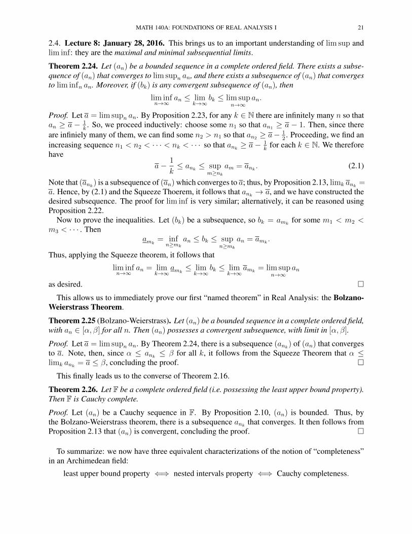
2.4. Lecture 8: January 28, 2016. This brings us to an important understanding of lim sup andlim inf: they are the maximal and minimal subsequential limits.
Theorem 2.24. Let (an) be a bounded sequence in a complete ordered field. There exists a subse-quence of (an) that converges to lim supn an, and there exists a subsequence of (an) that convergesto lim infn an. Moreover, if (bk) is any convergent subsequence of (an), then
lim infn→∞
an ≤ limk→∞
bk ≤ lim supn→∞
an.
Proof. Let a = lim supn an. By Proposition 2.23, for any k ∈ N there are infinitely many n so thatan ≥ a − 1
k. So, we proceed inductively: choose some n1 so that an1 ≥ a − 1. Then, since there
are infiniely many of them, we can find some n2 > n1 so that an2 ≥ a− 12. Proceeding, we find an
increasing sequence n1 < n2 < · · · < nk < · · · so that ank≥ a− 1
kfor each k ∈ N. We therefore
havea− 1
k≤ ank
≤ supm≥nk
am = ank. (2.1)
Note that (ank) is a subsequence of (an) which converges to a; thus, by Proposition 2.13, limk ank
=a. Hence, by (2.1) and the Squeeze Thoerem, it follows that ank
→ a, and we have constructed thedesired subsequence. The proof for lim inf is very similar; alternatively, it can be reasoned usingProposition 2.22.
Now to prove the inequalities. Let (bk) be a subsequence, so bk = amkfor some m1 < m2 <
m3 < · · · . Thenamk
= infn≥mk
an ≤ bk ≤ supn≥mk
an = amk.
Thus, applying the Squeeze theorem, it follows that
lim infn→∞
an = limk→∞
amk≤ lim
k→∞bk ≤ lim
k→∞amk
= lim supn→∞
an
as desired. �
This allows us to immediately prove our first “named theorem” in Real Analysis: the Bolzano-Weierstrass Theorem.
Theorem 2.25 (Bolzano-Weierstrass). Let (an) be a bounded sequence in a complete ordered field,with an ∈ [α, β] for all n. Then (an) possesses a convergent subsequence, with limit in [α, β].
Proof. Let a = lim supn an. By Theorem 2.24, there is a subsequence (ank) of (an) that converges
to a. Note, then, since α ≤ ank≤ β for all k, it follows from the Squeeze Theorem that α ≤
limk ank= a ≤ β, concluding the proof. �
This finally leads us to the converse of Theorem 2.16.
Theorem 2.26. Let F be a complete ordered field (i.e. possessing the least upper bound property).Then F is Cauchy complete.
Proof. Let (an) be a Cauchy sequence in F. By Proposition 2.10, (an) is bounded. Thus, bythe Bolzano-Weierstrass theorem, there is a subsequence ank
that converges. It then follows fromProposition 2.13 that (an) is convergent, concluding the proof. �
To summarize: we now have three equivalent characterizations of the notion of “completeness”in an Archimedean field:
least upper bound property ⇐⇒ nested intervals property ⇐⇒ Cauchy completeness.

22 TODD KEMP
We also know, by the half of Theorem 1.20 we’ve proved, that such a field is unique. So, to finallyprove the existence of R, it will suffice to give a construction of a Cauchy complete field that isArchimedean. The supplementary notes “Construction of R” describe how this is done in gorydetail.
Henceforth, we will deal with the field R, which satisfies all of the three equivalent complete-ness properties.
Now comfortably working in R, let us state a few more (standard) limit theorems.
Theorem 2.27 (Limit Theorems). Let (an) and (bn) be convergent sequences in R, with an → aand bn → b.
(1) The sequence cn = an + bn converges to a+ b.(2) The sequence dn = anbn converges to ab.(3) If b 6= 0, then bn 6= 0 for almost all n, and en = an
bnconverges to a
b.
Proof. For (1), choose Na, Nb ∈ N so that |an − a| < ε2
if n ≥ Na and |bn − b| < ε2
for n ≥ Nb.For any n ≥ N = max{Na, Nb}, we then have |cn − (a + b)| = |(an − a) + (bn − b)| ≤|an − a|+ |bn − b| < ε
2+ ε
2= ε, proving that limn cn = a+ b.
For (2), we need to be slightly more clever. Note that
|dn − ab| = |anbn − ab| = |anbn − anb+ anb− ab| ≤ |an||bn − b|+ |an − a||b|.By Proposition 2.10, there is some constant M > 0 so that |an| ≤ M for all n. So, for ε > 0, fixN1 large enough that |bn− b| < ε
2Mfor all n ≥ N1, and fix N2 large enough that |an− a| < ε
2|b| forall n ≥ N2. (If b = 0, we can take N2 to be any number we like.) Then for N = max{N1, N2}, ifn ≥ N we have
|dn − ab| ≤ |an||bn − b|+ |an − a||b| < M · ε
2M+
ε
2|b|· |b| = ε,
proving that limn dn = ab.For (3), first we need to show that (en) even makes sense. Note that en = an
bnis not well-defined
for any n for which bn = 0. But we’re only concerned about tails of sequences for limit statements,so once we’ve proven that bn 6= 0 for almost all n, we know that en is well-defined for all largen. For this, we use the assumption that b 6= 0, and so |b| > 0. Since limn bn = b, there is anN0 ∈ N so that, for n > N0, |bn − b| < |b|
2; i.e. − |b|
2< bn − b < |b|
2, and so bn < b + |b|
2and
also bn > b − |b|2
. Now, b 6= 0 so either b < 0 or b > 0. If b < 0, then |b| = −b in which casebn < b + |b|
2= b − b
2= b
2< 0; that is, for n > N0, bn < 0. If, on the other hand, b > 0, then
|b| = b, and so bn > b − |b|2
= b − b2= b
2> 0; that is, for n > N0, bn > 0. Thus, in all cases,
bn 6= 0 for n > N0, proving the first claim.For the limit statement, note that en = an · 1
bn. So, by (2), it suffices to show that 1
bn→ 1
b.
Compute that ∣∣∣∣ 1bn − 1
b
∣∣∣∣ = |bn − b||bn||b|.
As shown above, there is N0 so that, for n > N0, then bn > b2= |b|
2if bn > 0 and bn < b
2= − |b|
2if
bn < 0; i.e. this means that |bn| > |b|2
for n > N0. Hence, we have∣∣∣∣ 1bn − 1
b
∣∣∣∣ = |bn − b||bn||b|< 2|bn − b||b|2
, n > N0.
MATH 140A: FOUNDATIONS OF REAL ANALYSIS I 23
By assumption, bn → b, and so we can choose N ′ large enough that |bn − b| < |b|22ε for n > N ′.
Thus, letting N = max{N0, N′}, we have∣∣∣∣ 1bn − 1
b
∣∣∣∣ < 2|bn − b||b|2
<2
|b|2· |b|
2
2ε = ε, n > N.
This proves that 1bn→ 1
bas claimed. �
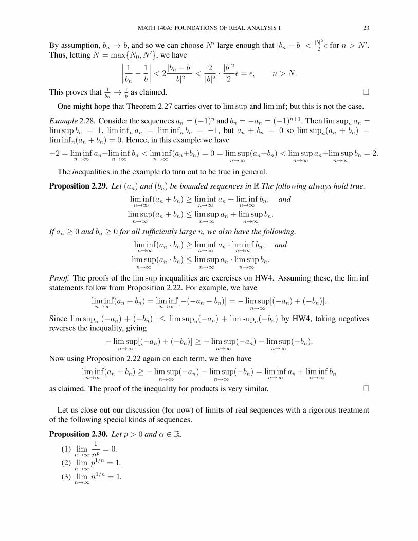
One might hope that Theorem 2.27 carries over to lim sup and lim inf; but this is not the case.
Example 2.28. Consider the sequences an = (−1)n and bn = −an = (−1)n+1. Then lim supn an =lim sup bn = 1, lim infn an = lim infn bn = −1, but an + bn = 0 so lim supn(an + bn) =lim infn(an + bn) = 0. Hence, in this example we have
−2 = lim infn→∞
an+lim infn→∞
bn < lim infn→∞
(an+bn) = 0 = lim supn→∞
(an+bn) < lim supn→∞
an+lim supn→∞
bn = 2.
The inequalities in the example do turn out to be true in general.
Proposition 2.29. Let (an) and (bn) be bounded sequences in R The following always hold true.
lim infn→∞
(an + bn) ≥ lim infn→∞
an + lim infn→∞
bn, and
lim supn→∞
(an + bn) ≤ lim supn→∞
an + lim supn→∞
bn.
If an ≥ 0 and bn ≥ 0 for all sufficiently large n, we also have the following.
lim infn→∞
(an · bn) ≥ lim infn→∞
an · lim infn→∞
bn, and
lim supn→∞
(an · bn) ≤ lim supn→∞
an · lim supn→∞
bn.
Proof. The proofs of the lim sup inequalities are exercises on HW4. Assuming these, the lim infstatements follow from Proposition 2.22. For example, we have
lim infn→∞
(an + bn) = lim infn→∞
[−(−an − bn)] = − lim supn→∞
[(−an) + (−bn)].
Since lim supn[(−an) + (−bn)] ≤ lim supn(−an) + lim supn(−bn) by HW4, taking negativesreverses the inequality, giving
− lim supn→∞
[(−an) + (−bn)] ≥ − lim supn→∞
(−an)− lim supn→∞
(−bn).
Now using Proposition 2.22 again on each term, we then have
lim infn→∞
(an + bn) ≥ − lim supn→∞
(−an)− lim supn→∞
(−bn) = lim infn→∞
an + lim infn→∞
bn
as claimed. The proof of the inequality for products is very similar. �
Let us close out our discussion (for now) of limits of real sequences with a rigorous treatmentof the following special kinds of sequences.
Proposition 2.30. Let p > 0 and α ∈ R.
(1) limn→∞
1
np= 0.
(2) limn→∞
p1/n = 1.
(3) limn→∞
n1/n = 1.
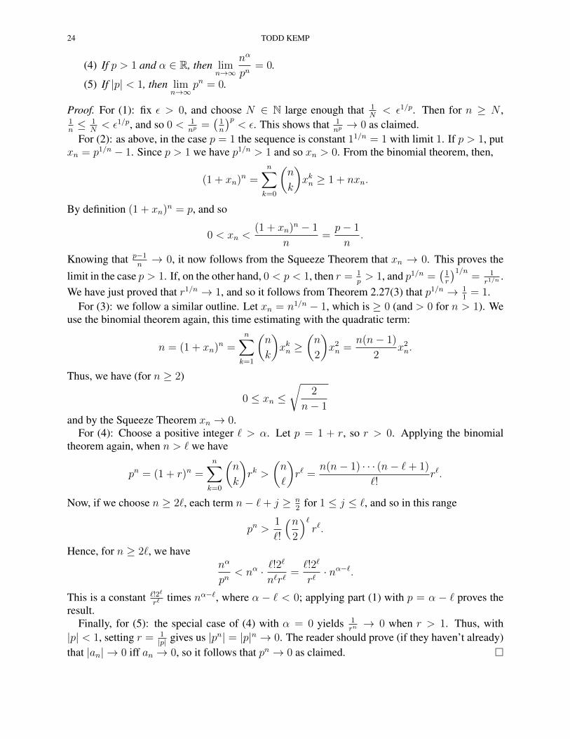
24 TODD KEMP
(4) If p > 1 and α ∈ R, then limn→∞
nα
pn= 0.
(5) If |p| < 1, then limn→∞
pn = 0.
Proof. For (1): fix ε > 0, and choose N ∈ N large enough that 1N< ε1/p. Then for n ≥ N ,
1n≤ 1
N< ε1/p, and so 0 < 1
np =(1n
)p< ε. This shows that 1
np → 0 as claimed.For (2): as above, in the case p = 1 the sequence is constant 11/n = 1 with limit 1. If p > 1, put
xn = p1/n − 1. Since p > 1 we have p1/n > 1 and so xn > 0. From the binomial theorem, then,
(1 + xn)n =
n∑k=0
(n
k
)xkn ≥ 1 + nxn.
By definition (1 + xn)n = p, and so
0 < xn <(1 + xn)
n − 1
n=p− 1
n.
Knowing that p−1n→ 0, it now follows from the Squeeze Theorem that xn → 0. This proves the
limit in the case p > 1. If, on the other hand, 0 < p < 1, then r = 1p> 1, and p1/n =
(1r
)1/n= 1
r1/n.
We have just proved that r1/n → 1, and so it follows from Theorem 2.27(3) that p1/n → 11= 1.
For (3): we follow a similar outline. Let xn = n1/n − 1, which is ≥ 0 (and > 0 for n > 1). Weuse the binomial theorem again, this time estimating with the quadratic term:
n = (1 + xn)n =
n∑k=1
(n
k
)xkn ≥
(n
2
)x2n =
n(n− 1)
2x2n.
Thus, we have (for n ≥ 2)
0 ≤ xn ≤√
2
n− 1and by the Squeeze Theorem xn → 0.
For (4): Choose a positive integer ` > α. Let p = 1 + r, so r > 0. Applying the binomialtheorem again, when n > ` we have
pn = (1 + r)n =n∑k=0
(n
k
)rk >
(n
`
)r` =
n(n− 1) · · · (n− `+ 1)
`!r`.
Now, if we choose n ≥ 2`, each term n− `+ j ≥ n2
for 1 ≤ j ≤ `, and so in this range
pn >1
`!
(n2
)`r`.
Hence, for n ≥ 2`, we havenα
pn< nα · `!2
`
n`r`=`!2`
r`· nα−`.
This is a constant `!2`
r`times nα−`, where α − ` < 0; applying part (1) with p = α − ` proves the
result.Finally, for (5): the special case of (4) with α = 0 yields 1
rn→ 0 when r > 1. Thus, with
|p| < 1, setting r = 1|p| gives us |pn| = |p|n → 0. The reader should prove (if they haven’t already)
that |an| → 0 iff an → 0, so it follows that pn → 0 as claimed. �
MATH 140A: FOUNDATIONS OF REAL ANALYSIS I 25
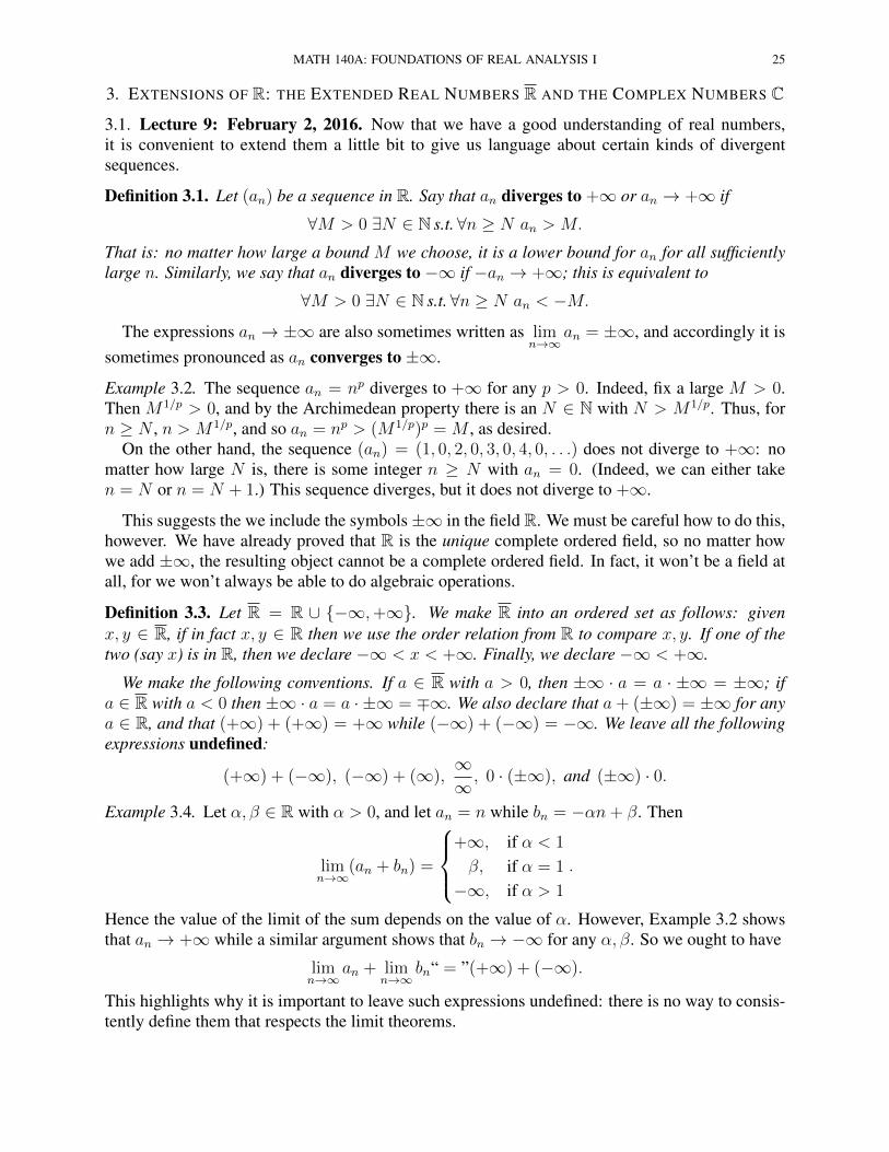
3. EXTENSIONS OF R: THE EXTENDED REAL NUMBERS R AND THE COMPLEX NUMBERS C
3.1. Lecture 9: February 2, 2016. Now that we have a good understanding of real numbers,it is convenient to extend them a little bit to give us language about certain kinds of divergentsequences.
Definition 3.1. Let (an) be a sequence in R. Say that an diverges to +∞ or an → +∞ if
∀M > 0 ∃N ∈ N s.t.∀n ≥ N an > M.
That is: no matter how large a bound M we choose, it is a lower bound for an for all sufficientlylarge n. Similarly, we say that an diverges to −∞ if −an → +∞; this is equivalent to
∀M > 0 ∃N ∈ N s.t.∀n ≥ N an < −M.
The expressions an → ±∞ are also sometimes written as limn→∞
an = ±∞, and accordingly it issometimes pronounced as an converges to ±∞.
Example 3.2. The sequence an = np diverges to +∞ for any p > 0. Indeed, fix a large M > 0.Then M1/p > 0, and by the Archimedean property there is an N ∈ N with N > M1/p. Thus, forn ≥ N , n > M1/p, and so an = np > (M1/p)p =M , as desired.
On the other hand, the sequence (an) = (1, 0, 2, 0, 3, 0, 4, 0, . . .) does not diverge to +∞: nomatter how large N is, there is some integer n ≥ N with an = 0. (Indeed, we can either taken = N or n = N + 1.) This sequence diverges, but it does not diverge to +∞.
This suggests the we include the symbols±∞ in the field R. We must be careful how to do this,however. We have already proved that R is the unique complete ordered field, so no matter howwe add ±∞, the resulting object cannot be a complete ordered field. In fact, it won’t be a field atall, for we won’t always be able to do algebraic operations.
Definition 3.3. Let R = R ∪ {−∞,+∞}. We make R into an ordered set as follows: givenx, y ∈ R, if in fact x, y ∈ R then we use the order relation from R to compare x, y. If one of thetwo (say x) is in R, then we declare −∞ < x < +∞. Finally, we declare −∞ < +∞.
We make the following conventions. If a ∈ R with a > 0, then ±∞ · a = a · ±∞ = ±∞; ifa ∈ R with a < 0 then ±∞ · a = a · ±∞ = ∓∞. We also declare that a+ (±∞) = ±∞ for anya ∈ R, and that (+∞) + (+∞) = +∞ while (−∞) + (−∞) = −∞. We leave all the followingexpressions undefined:
(+∞) + (−∞), (−∞) + (∞),∞∞, 0 · (±∞), and (±∞) · 0.
Example 3.4. Let α, β ∈ R with α > 0, and let an = n while bn = −αn+ β. Then
limn→∞
(an + bn) =
+∞, if α < 1
β, if α = 1
−∞, if α > 1
.
Hence the value of the limit of the sum depends on the value of α. However, Example 3.2 showsthat an → +∞ while a similar argument shows that bn → −∞ for any α, β. So we ought to have
limn→∞
an + limn→∞
bn“ = ”(+∞) + (−∞).
This highlights why it is important to leave such expressions undefined: there is no way to consis-tently define them that respects the limit theorems.

26 TODD KEMP
We can also use these conventions to extend the notions of sup and inf to unbounded sets, andthe notions of lim sup and lim inf to unbounded sequences.
Definition 3.5. Let E ⊆ R be any nonempty subset. If E is not bounded above, declare supE =+∞; ifE is not bounded below, declare inf E = −∞. We also make the convention that sup(∅) =−∞ while inf(∅) = +∞. (Note: this means that, in the one special case E = ∅, it is not truethat inf E ≤ supE.)
Similarly, let (an) be any sequence in R. If (an) is not bounded above, declare lim supn an =+∞; if (an) is not bounded below, declare lim infn an = −∞.
With these conventions, essentially all of the theorems involving limits extend to unboundedsequences.
Proposition 3.6. Using the preceding conventions, Lemma 2.4, Proposition 2.6, Proposition 2.13(2),Squeeze Theorem 2.14, Proposition 2.21, Proposition 2.22, and Theorem 2.24 all generalize to thecases where the limits in the statements are allowed to be in R rather than just R. Moreover, Theo-rem 2.27 and Proposition 2.29 also hold in this more general setting whenever the statements makesense: i.e. excluding the cases when the involved expressions are undefined (like (+∞) + (−∞)).
Proof. It would take many pages to prove all of the special cases of all of these results remain validin the extended reals. Let us choose just one to illustrate: Theorem 2.27(1): if limn an = a andlimn bn = b, then limn(an + bn) = a + b. We already know this holds true when a, b ∈ R. Ifa = +∞ and b = −∞, or a = −∞ and b = +∞, the sum a + b is undefined, and so we excludethese cases from the statement of the theorem. So we only need to consider the cases that a ∈ Rand b = ±∞, a = ±∞ and b ∈ R, or a = b = ±∞.
• a ∈ R and b = +∞: Since (an) is convergent in R, it is bounded; thus say |an| ≤ L. ThenfixM > 0 and chooseN so that bn > M+L for n ≥ N . Thus an+bn > −L+(M+L) =M for n ≥ N , and so an + bn → +∞. The argument is similar when b = −∞.• a = ±∞ and b ∈ R: this is the same as the previous case, just reverse the roles of an andbn and a and b.• a = b = +∞: let M > 0, and choose N1 so that an > M/2 for n ≥ N1; chooseN2 so that bn > M/2 for n ≥ N2. Thus, for n ≥ N = max{N1, N2}, it follows thatan + bn ≥ M/2 +M/2 = M , proving that an + bn → +∞ as required. The argumentwhen a = b = −∞ is very similar.
�
Now we turn to a very different extension of R: the Complex Numbers. We’ve already discussedthem a little bit, in Example 1.12(3-3.5) and HW1.4, so we’ll start by reiterating that discussion.We will rely on our knowledge of linear algebra.
Definition 3.7. Let C denote the following set of 2× 2 matrices over R:
C =
{[a −bb a
]: a, b ∈ R
}.
Then C = spanR{I, J}, where
I =
[1 00 1
], J =
[0 −11 0
].
MATH 140A: FOUNDATIONS OF REAL ANALYSIS I 27
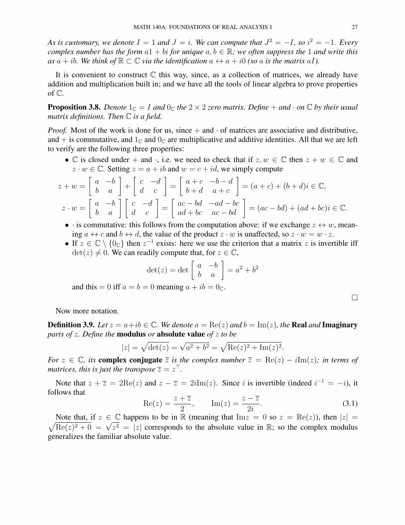
As is customary, we denote I = 1 and J = i. We can compute that J2 = −I , so i2 = −1. Everycomplex number has the form a1 + bi for unique a, b ∈ R; we often suppress the 1 and write thisas a+ ib. We think of R ⊂ C via the identification a↔ a+ i0 (so a is the matrix aI).
It is convenient to construct C this way, since, as a collection of matrices, we already haveaddition and multiplication built in; and we have all the tools of linear algebra to prove propertiesof C.
Proposition 3.8. Denote 1C = I and 0C the 2× 2 zero matrix. Define + and · on C by their usualmatrix definitions. Then C is a field.
Proof. Most of the work is done for us, since + and · of matrices are associative and distributive,and + is commutative, and 1C and 0C are multiplicative and additive identities. All that we are leftto verify are the following three properties:
• C is closed under + and ·, i.e. we need to check that if z, w ∈ C then z + w ∈ C andz · w ∈ C. Setting z = a+ ib and w = c+ id, we simply compute
z + w =
[a −bb a
]+
[c −dd c
]=
[a+ c −b− db+ d a+ c
]= (a+ c) + (b+ d)i ∈ C,
z · w =
[a −bb a
] [c −dd c
]=
[ac− bd −ad− bcad+ bc ac− bd
]= (ac− bd) + (ad+ bc)i ∈ C.
• · is commutative: this follows from the computation above: if we exchange z ↔ w, mean-ing a↔ c and b↔ d, the value of the product z · w is unaffected, so z · w = w · z.• If z ∈ C \ {0C} then z−1 exists: here we use the criterion that a matrix z is invertible iffdet(z) 6= 0. We can readily compute that, for z ∈ C,
det(z) = det
[a −bb a
]= a2 + b2
and this = 0 iff a = b = 0 meaning a+ ib = 0C.�
Now more notation.
Definition 3.9. Let z = a+ib ∈ C. We denote a = Re(z) and b = Im(z), the Real and Imaginaryparts of z. Define the modulus or absolute value of z to be
|z| =√
det(z) =√a2 + b2 =
√Re(z)2 + Im(z)2.
For z ∈ C, its complex conjugate z is the complex number z = Re(z) − iIm(z); in terms ofmatrices, this is just the transpose z = z>.
Note that z + z = 2Re(z) and z − z = 2iIm(z). Since i is invertible (indeed i−1 = −i), itfollows that
Re(z) =z + z
2, Im(z) =
z − z2i
. (3.1)
Note that, if z ∈ C happens to be in R (meaning that Imz = 0 so z = Re(z)), then |z| =√Re(z)2 + 0 =
√z2 = |z| corresponds to the absolute value in R; so the complex modulus
generalizes the familiar absolute value.
28 TODD KEMP
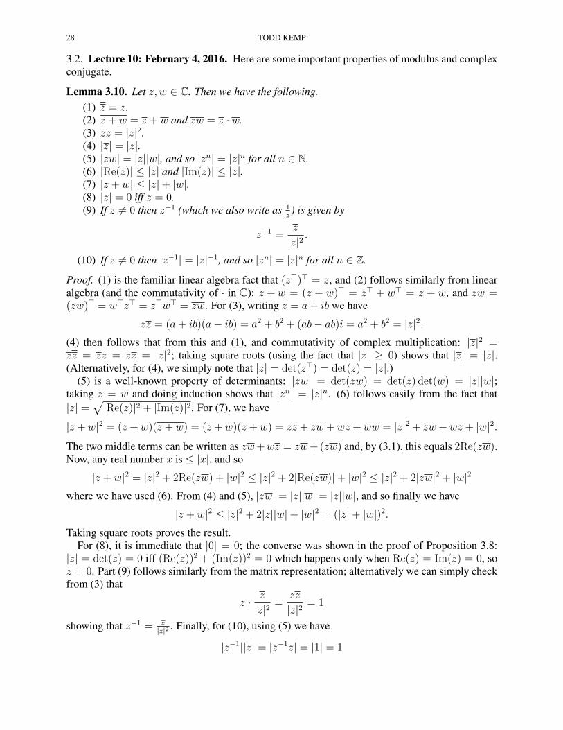
3.2. Lecture 10: February 4, 2016. Here are some important properties of modulus and complexconjugate.
Lemma 3.10. Let z, w ∈ C. Then we have the following.(1) z = z.(2) z + w = z + w and zw = z · w.(3) zz = |z|2.(4) |z| = |z|.(5) |zw| = |z||w|, and so |zn| = |z|n for all n ∈ N.(6) |Re(z)| ≤ |z| and |Im(z)| ≤ |z|.(7) |z + w| ≤ |z|+ |w|.(8) |z| = 0 iff z = 0.(9) If z 6= 0 then z−1 (which we also write as 1
z) is given by
z−1 =z
|z|2.
(10) If z 6= 0 then |z−1| = |z|−1, and so |zn| = |z|n for all n ∈ Z.
Proof. (1) is the familiar linear algebra fact that (z>)> = z, and (2) follows similarly from linearalgebra (and the commutativity of · in C): z + w = (z + w)> = z> + w> = z + w, and zw =(zw)> = w>z> = z>w> = zw. For (3), writing z = a+ ib we have
zz = (a+ ib)(a− ib) = a2 + b2 + (ab− ab)i = a2 + b2 = |z|2.(4) then follows that from this and (1), and commutativity of complex multiplication: |z|2 =zz = zz = zz = |z|2; taking square roots (using the fact that |z| ≥ 0) shows that |z| = |z|.(Alternatively, for (4), we simply note that |z| = det(z>) = det(z) = |z|.)
(5) is a well-known property of determinants: |zw| = det(zw) = det(z) det(w) = |z||w|;taking z = w and doing induction shows that |zn| = |z|n. (6) follows easily from the fact that|z| =
√|Re(z)|2 + |Im(z)|2. For (7), we have
|z +w|2 = (z +w)(z + w) = (z +w)(z +w) = zz + zw +wz +ww = |z|2 + zw +wz + |w|2.
The two middle terms can be written as zw+wz = zw+(zw) and, by (3.1), this equals 2Re(zw).Now, any real number x is ≤ |x|, and so
|z + w|2 = |z|2 + 2Re(zw) + |w|2 ≤ |z|2 + 2|Re(zw)|+ |w|2 ≤ |z|2 + 2|zw|2 + |w|2
where we have used (6). From (4) and (5), |zw| = |z||w| = |z||w|, and so finally we have
|z + w|2 ≤ |z|2 + 2|z||w|+ |w|2 = (|z|+ |w|)2.Taking square roots proves the result.
For (8), it is immediate that |0| = 0; the converse was shown in the proof of Proposition 3.8:|z| = det(z) = 0 iff (Re(z))2 + (Im(z))2 = 0 which happens only when Re(z) = Im(z) = 0, soz = 0. Part (9) follows similarly from the matrix representation; alternatively we can simply checkfrom (3) that
z · z
|z|2=
zz
|z|2= 1
showing that z−1 = z|z|2 . Finally, for (10), using (5) we have
|z−1||z| = |z−1z| = |1| = 1
MATH 140A: FOUNDATIONS OF REAL ANALYSIS I 29
so |z|−1 = |z−1|. An induction argument combining this with (5) shows that |z|−n = |z−n| forn ∈ N, and coupling this with the second statement of (5) concludes the proof. �
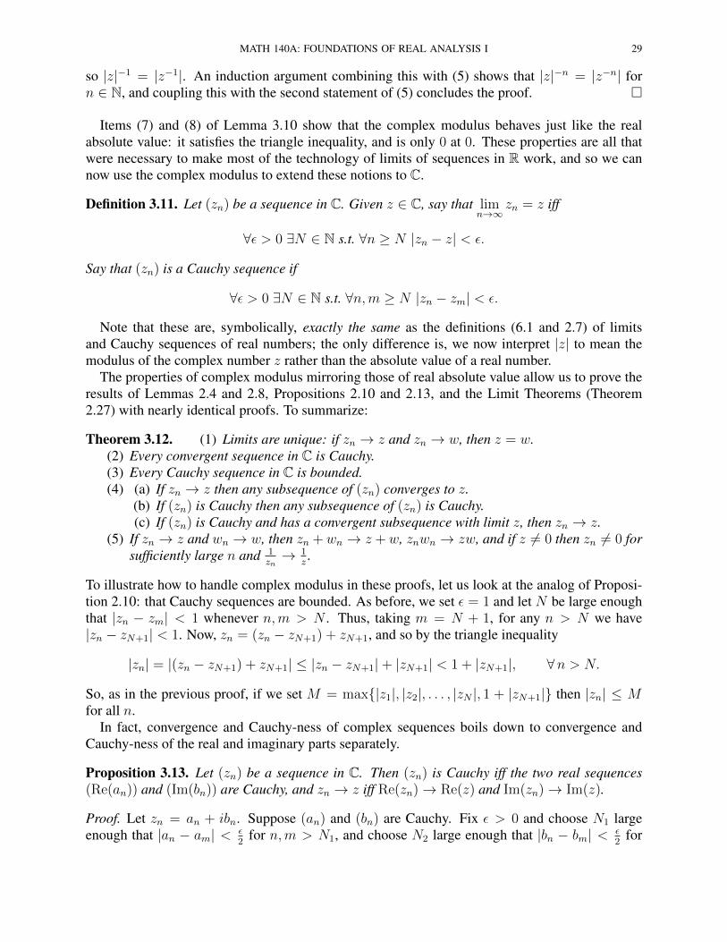
Items (7) and (8) of Lemma 3.10 show that the complex modulus behaves just like the realabsolute value: it satisfies the triangle inequality, and is only 0 at 0. These properties are all thatwere necessary to make most of the technology of limits of sequences in R work, and so we cannow use the complex modulus to extend these notions to C.
Definition 3.11. Let (zn) be a sequence in C. Given z ∈ C, say that limn→∞
zn = z iff
∀ε > 0 ∃N ∈ N s.t. ∀n ≥ N |zn − z| < ε.
Say that (zn) is a Cauchy sequence if
∀ε > 0 ∃N ∈ N s.t. ∀n,m ≥ N |zn − zm| < ε.
Note that these are, symbolically, exactly the same as the definitions (6.1 and 2.7) of limitsand Cauchy sequences of real numbers; the only difference is, we now interpret |z| to mean themodulus of the complex number z rather than the absolute value of a real number.
The properties of complex modulus mirroring those of real absolute value allow us to prove theresults of Lemmas 2.4 and 2.8, Propositions 2.10 and 2.13, and the Limit Theorems (Theorem2.27) with nearly identical proofs. To summarize:
Theorem 3.12. (1) Limits are unique: if zn → z and zn → w, then z = w.(2) Every convergent sequence in C is Cauchy.(3) Every Cauchy sequence in C is bounded.(4) (a) If zn → z then any subsequence of (zn) converges to z.
(b) If (zn) is Cauchy then any subsequence of (zn) is Cauchy.(c) If (zn) is Cauchy and has a convergent subsequence with limit z, then zn → z.
(5) If zn → z and wn → w, then zn +wn → z +w, znwn → zw, and if z 6= 0 then zn 6= 0 forsufficiently large n and 1
zn→ 1
z.
To illustrate how to handle complex modulus in these proofs, let us look at the analog of Proposi-tion 2.10: that Cauchy sequences are bounded. As before, we set ε = 1 and let N be large enoughthat |zn − zm| < 1 whenever n,m > N . Thus, taking m = N + 1, for any n > N we have|zn − zN+1| < 1. Now, zn = (zn − zN+1) + zN+1, and so by the triangle inequality
|zn| = |(zn − zN+1) + zN+1| ≤ |zn − zN+1|+ |zN+1| < 1 + |zN+1|, ∀n > N.
So, as in the previous proof, if we set M = max{|z1|, |z2|, . . . , |zN |, 1 + |zN+1|} then |zn| ≤ Mfor all n.
In fact, convergence and Cauchy-ness of complex sequences boils down to convergence andCauchy-ness of the real and imaginary parts separately.
Proposition 3.13. Let (zn) be a sequence in C. Then (zn) is Cauchy iff the two real sequences(Re(an)) and (Im(bn)) are Cauchy, and zn → z iff Re(zn)→ Re(z) and Im(zn)→ Im(z).
Proof. Let zn = an + ibn. Suppose (an) and (bn) are Cauchy. Fix ε > 0 and choose N1 largeenough that |an − am| < ε
2for n,m > N1, and choose N2 large enough that |bn − bm| < ε
2for

30 TODD KEMP
n,m > N2. Then for n,m > N = max{N1, N2}, we have
|zn − zm| = |(an + ibn)− (am + ibm)| = |(an − am) + i(bn − bm)| ≤ |an − am|+ |i(bn − bm)|= |an − am|+ |bn − bm|
<ε
2+ε
2= ε
where, in the second last step, we used the fact that |i(bn − bm)| = |i||bn − bm| and |i| = 1. Thus,(zn) is Cauchy. For the converse, suppose that (zn) is Cauchy. Fix ε > 0, and choose N largeenough that |zn − zm| < ε for n,m > N . Then we also have
|Re(zn)− Re(zm)| = |Re(zn − zm)| ≤ |zn − zm| < ε, and
|Im(zn)− Im(zm)| = |Im(zn − zm)| ≤ |zn − zm| < ε
for n,m > N . Thus, both (Re(zn)) and (Im(zn)) are Cauchy, as claimed.The proof of the limit statements is very similar, and is left as a homework exercise (on HW6).
�
Now, C is not an ordered field (you proved this on HW1), so it does not even make sense to askif it has the least upper bound property (and likewise we cannot talk about a Squeeze Theorem,or lim sup and lim inf). This is one of the main reasons we gave an equivalent characterization ofthe least upper bound property – Cauchy completeness – that does not explicitly require an orderrelation.
Theorem 3.14. The field C is Cauchy complete: any Cauchy sequence is convergent.
Proof. Let (zn) be a Cauchy sequence in C. By Proposition 3.13, the two real sequences (Re(zn))and (Im(zn)) are both Cauchy. Since R is Cauchy complete, it follows that there are real numbersa, b ∈ R so that Re(zn) → a and Im(zn) → b. It then follows, again by Proposition 3.13, thatzn → a+ ib. �
In R, we proved the Bolzano-Weierstrass theorem (that bounded sequences have convergentsubsequences) using the technology of lim sup and lim inf. As noted, since C is not ordered, thereis no way to talk about lim sup and lim inf for a complex sequence. Nevertheless, the Bolzano-Weierstrass theorem holds true in C. We conclude our discussion of C (for now) with its proof.
Theorem 3.15 (Bolzano-Weierstrass). Every bounded sequence in C contains a convergent sub-sequence.
Proof. Let (zn) be a bounded sequence. Letting zn = an+ ibn, since |an| ≤ |zn| and |bn| ≤ |zn|, itfollows that (an) and (bn) are bounded sequences in R. Now, by the Bolzano-Weierstrass theoremfor R, there is a subsequence ank
of (an) that converges to some real number a. Consider now thesubsequence bnk
of (bn). Since (bn) is bounded, so is (bnk), and so again applying the Bolzano-
Weierstrass theorem for R, there is a further subsequence (bnk`) that converges to some b ∈ R. The
subsequence (ank`) is a subsequence of the convergent sequence ank
and hence also converges toa. Thus, by Propostion 3.13, the subsequence znk`
converges to a+ ib as `→∞. �
Remark 3.16. This proof highlights an important technique with subsequences in higher dimen-sional spaces. We chose the second subsequence as a subsubsequence, not only a subsequence.Had we tried to select the subsequences of the real and imaginary parts independently, we could nothave concluded anything about the two together. Indeed, the Bolzano-Weierstrass theorem givesus a convergent subsequence ank
and also gives us a convergent subsequence bmk. But we need to
MATH 140A: FOUNDATIONS OF REAL ANALYSIS I 31
use the same index n for both an and bn, which might not be possible with independent choiceslike this. A priori, the chosen convergent subsequence of an might have been (a1, a3, a5, . . .), whilefrom bn we might have chosen (b2, b4, b6, . . .), ne’er the ’tween shall meet.
32 TODD KEMP
4. SERIES
4.1. Lecture 11: February 9, 2016. We now turn to a special class of sequences called series.
Definition 4.1. Let (an) be a sequence in R or C. The series associated to (an) is the new sequence(sn) given by
sn =n∑k=1
ak = a1 + a2 + · · ·+ an.
It is a bit of a misnomer to refer to series as special kinds of sequences; indeed, any sequence isthe series associated to some other sequence. For let (an) be a sequence. Define a new sequence(bn) by
b1 = a1, bn = an − an−1 for n > 1.
Then a1 = b1 =∑1
k=1 bk, and for n > 1 we compute thatn∑k=1
bk = b1 + b2 + · · ·+ bk = a1 + (a2 − a1) + (a3 − a2) + · · ·+ (an − an−1) = an.
Thus, (an) (the arbitrary sequence we started with) is the series associated to the sequence (bn).We will see, however, that the concept of convergence is quite different when applied to the
series associated to a sequence rather than the sequence itself.
Definition 4.2. Let (an) be a sequence in R or C, and let sn =∑n
k=1 ak be its series. We say thatthe series converges if the sequence (sn) converges. If the limit is s = limn→∞ sn, we denote it by
s =∞∑n=1
an = limn→∞
n∑k=1
ak.
In this case, we will often use the cumbersome-but-standard notation “the series∑∞
n=1 an con-verges”.
Example 4.3 (Geometric Series). Let r ∈ C, and consider the sequence an = rn (in this case itis customary to start at n = 0). We can compute the terms in the series exactly, following a trickpurportedly invented by Gauss at age 10.
sn =n∑k=0
ak = 1 + r + r2 + · · ·+ rn.
∴ rsn = r + r2 + · · ·+ rn + rn+1.
So, subtracting the two lines, we have
(1− r)sn = sn − rsn = 1− rn+1.
Now, if r = 1, this gives no information. In that degenerate case, we simply have sn = 1 + 1 +· · ·+ 1 = n, and this series does not converge. In all other cases, we have the explicit formula
sn =1− rn+1
1− r.
Using the limit theorems, we can decide whether this converges, and to what, just looking at theshifted sequence an+1 = rn+1. If |r| < 1, then this converges to 0. If |r| ≥ 1, this sequence does

MATH 140A: FOUNDATIONS OF REAL ANALYSIS I 33
not converge. (This is something you should work out.) Thus, we have∞∑n=0
rn =1
1− r, if |r| < 1
while the series diverges if |r| ≥ 1.
Example 4.4. Consider the sequence an = 1n(n+1)
. We can employ a trick here: the partial fractionsdecomposition:
1
n(n+ 1)=
1
n− 1
n+ 1.
Thus, taking the series sn =∑n
k=1 an, we have
sn =n∑k=1
1
k(k + 1)=
n∑k=1
(1
k− 1
k + 1
)=
(1− 1
2
)+
(1
2− 1
3
)+ · · ·+
(1
n− 1
n+ 1
).
This is a telescoping sum: all terms except for the first and the last cancel in pairs. Thus, we havea closed formula
sn = 1− 1
n+ 1.
Hence, the series converges, and we have explicitly∞∑n=1
= limn→∞
sn = limn→∞
(1− 1
n+ 1
)= 1.
Example 4.5 (Harmonic Series). Consider the series sn =∑n
k=11k. That is
sn = 1 +1
2+
1
3+ · · ·+ 1
n.
If you add up the first billion terms (i.e. s109) you get about 21.3. This seems to suggest conver-gence; after all, the terms are getting arbitrarily small. However, this series does not converge. Tosee why, look at terms sN with N = 2m+2m−1 + · · ·+2+1 for some positive integer m. (By theway, from the previous example, this could be written explicitly as N = 2m+1 − 1.) Then we cangroup terms as
sN = (1) +
(1
2+
1
3
)+
(1
4+
1
5+
1
6+
1
7
)+ · · ·+
(1
2m + 1+
1
2m + 2+ · · ·+ 1
2m+1 − 1
).
That is: we break up the sum into m+1 groups, the first group with 1 term, the second with 2, thethird with 4, up to the last with 2m terms. Now, 1 > 1
2. In the sec ond group of terms, both 1
2and 1
3
are > 14. In the next group, each of the four terms is > 1
8. That is, we have
sN >
(1
2
)+
(1
4+
1
4
)+
(1
8+
1
8+
1
8+
1
8
)+ · · ·+
(1
2m+1+
1
2m+1+ · · ·+ 1
2m+1
)=
1
2+
1
2+
1
2+ · · ·+ 1
2=m+ 1
2.
Now, sn+1 = sn +1
n+1≥ sn, so (sn) is an increasing sequence. We’ve just shown that, for any
integer m, we can find some time N so that sN ≥ m+12
, and so it follows that for all larger n ≥ N ,sn ≥ sN ≥ m+1
2. Since m+1
2is arbitrarily larger, we’ve just proved that sn → +∞ as n→∞. So
the series diverges.

34 TODD KEMP
In Example 4.3, we were able to compute the nth term in the series as a closed formula, andcompute the limit directly. It is rare that we can do this explicitly; more often, we will need tomake estimates like we did in Example 4.5. So we now begin to discuss some general tools forattacking such limits.
Proposition 4.6 (Cauchy Criterion). Let an be a sequence in R or C. Then the series∑∞
n=1 anconverges if and only if: for every ε > 0, there is a natural number N ∈ N so that, for allm ≥ n ≥ N , ∣∣∣∣∣
m∑k=n+1
ak
∣∣∣∣∣ < ε.
Proof. This is just a restatement of the Cauchy completeness of R and C. Let sn =∑n
k=1 ak. Then
m∑k=n+1
= an+1 + · · ·+ am = sm − sn.
Thus, having decided to always use m to denote the larger of m,n, the statement is that, for everyε > 0 there is N ∈ N such that, for m ≥ n ≥ N , |sm − sn| < ε; this is precisely the statement that(sn) is a Cauchy sequence. In R or C, this is equivalent to (sn) being convergent, as desired. �
Corollary 4.7. Let (an) be a sequence such that the series∑∞
n=1 an converges. Then an → 0.
Proof. By the Cauchy Criterion (Proposition 4.6), given ε > 0 we may find N ∈ N so that (lettingn = m− 1) for m > N ,
ε >
∣∣∣∣∣∣m∑
k=(m−1)+1
ak
∣∣∣∣∣∣ = |am|.This is precisely the statement that am → 0 as m→∞. �
As Example 4.5 points out, the converse to Corollary 4.7 is false: there are sequences, such asan = 1
n, that tend to 0, but for which the series
∑∞n=1 an diverges.
It is often impossible to compute the exact value of the sum∑∞
n=1 an of a convergent series.More often, we use estimates to approximate the value. More basically, we use estimates to de-termine whether the series converges or not, without any direct knowledge of the value if it doesconverge. The most basic test for convergence is the comparison theorem.
Theorem 4.8 (Comparison). Let (an) and (bn) be sequences in C.
(1) If bn ≥ 0 and∑
n bn converges, and if |an| ≤ bn for all sufficiently large n, then∑
n anconverges, and |
∑n an| ≤
∑n bn.
(2) If an ≥ bn ≥ 0 for all sufficiently large n and∑
n bn diverges, then∑
n an diverges.
Proof. For item 1: by assumption∑
n bn converges, and so by the Cauchy criterion, for given ε > 0we can choose N0 ∈ N so that, for m ≥ n ≥ N0,
m∑k=n+1
bk < ε
MATH 140A: FOUNDATIONS OF REAL ANALYSIS I 35
(here we have used the fact that bn ≥ 0 to drop the modulus). Now, let N1 be large enough that|an| ≤ bn for n ≥ N1. Then for m ≥ n ≥ max{N0, N1}, we have∣∣∣∣∣
m∑k=n+1
ak
∣∣∣∣∣ ≤m∑
k=n+1
|ak| ≤m∑
k=n+1
bk < ε.
So the series∑
n an satisfies the Cauchy criterion, and therefore is convergent.Item 2 follows from item 1 by contrapositive: if
∑n an converges, then since bn = |bn| ≤ an for
all large n, we have just proven that∑
n bn converges. Thus, if∑
n bn diverges, so must∑
n an. �
Example 4.9. The series∑
n1√n
diverges, since 1√n≥ 1
nand, by Example 4.5,
∑n
1n
diverges. Onthe other hand, note that
n2 =1
2n2 +
1
2n2 ≥ 1
2n2 +
1
2n =
1
2n(n+ 1)
for n ≥ 1. Thus 1n2 ≤ 2
n(n+1). As we computed in Example 4.4,
∑∞n=1
1n(n+1)
= 1, so by the limittheorems,
∑∞n=1
2n(n+1)
= 2. That is: this series converges. It follows from the comparison testthat
∑∞n=1
1n2 converges.
In showing that the harmonic series diverges, we broke the terms up into groups of exponentiallyincreasing size. This is an important trick known as the lacunary technique, and it works wellwhen the sequence of terms is positive and decreasing.
Proposition 4.10 (Lacunary Series). Suppose (an) is a sequence of non-negative numbers that isdecreasing: an ≥ an+1 ≥ 0 for all n. Then
∑∞n=1 an converges if and only if the series
∞∑k=0
2ka2k = a1 + 2a2 + 4a4 + 8a8 + · · ·
converges.
Proof. Since ak ≥ 0 for all k, the series of partial sums sn =∑n
k=1 ak is monotone increasing.Hence, convergence of sn is equivalent to the boundedness of (sn). Let tk = a1 + 2a2 + 4a4 +· · ·+ 2kak. We will show that (sn) is bounded iff (tk) is bounded.
Note that 2k ≤ 2k+1 − 1, and so if n < 2k then n < 2k+1 − 1. Then we have for such n
sn = a1 + a2 + a3 + · · ·+ an ≤ a1 + a2 + a3 + · · ·+ a2k+1−1
= (a1) + (a2 + a3) + · · ·+ (a2k + · · ·+ a2k+1−1)
≤ a1 + 2a2 + · · ·+ 2ka2k = tk.
(In the last inequality, we used the fact that an is decreasing.) This shows that if (tk) is bounded,then so is (sn). For the converse, we just group terms slightly differently (exactly as we did in theproof of the divergence of the harmonic series): if n > 2k, then
sn = a1 + a2 + a3 + · · ·+ an ≥ a1 + a2 + a3 + · · ·+ a2k
= (a1) + (a2) + (a3 + a4) + · · ·+ (a2k−1+1 + · · ·+ a2k)
≥ 1
2a1 + a2 + 2a4 · · ·+ 2k−1a2k =
1
2tk.
Thus tk ≤ 2sn whenever n > 2k. This shows that if (sn) is bounded then so is (tk), concluding theproof. �
36 TODD KEMP
Example 4.11. Let p ∈ R, and consider the series∑∞
n=11np . We’ve already seen that this series
diverges when p = 1. If p < 1, then 1np ≥ 1
n; it follows by the comparison theorem that the series∑∞
n=11np diverges for p ≤ 1.
On the other hand, consider p > 1. Here the sequence of terms an = 1np is positive and
decreasing, so we may use the lacunary series test to determine whether the series converges.Compute that
∞∑k=0
2ka2k =∞∑k=0
2k1
2kp=∞∑k=0
2(1−p)k.
This is a geometric series, with base r = 21−p. So 0 < r < 1 provided that p > 1, in whichcase the series converges. Hence, by Proposition 4.10, the series
∑∞n=1
1np converges if and only if
p > 1.

MATH 140A: FOUNDATIONS OF REAL ANALYSIS I 37
4.2. Lecture 12: February 11, 2016. Two generally effective tools for deciding convergence,that you already saw in your calculus class, are the Root Test and the Ratio Test. Both of them arepredicated on rough comparison with a geometric series, cf. Example 4.3. If an = rn, then
∑n an
converges iff |r| < 1. Now, note for this series that this important constant |r| can be computedeither as |an|1/n or as |an+1
an|. Even when these quantities are not constant, they still can give a lot
of information about the convergence of the series.
Theorem 4.12 (Root Test). Let (an) be a sequence in C. Define
α = lim supn→∞
|an|1/n.
If α < 1, then∑
n an converges. If α > 1, then∑
n an diverges.
Remark 4.13. It is important to note that the theorem gives no information when α = 1. Indeed,consider Examples 4.5 and 4.9, showing that
∑∞n=1
1n
diverges, while∑∞
n=11n2 converges. But, in
both cases, we have
limn→∞
(1
n
)1/n
= limn→∞
(1
n2
)1/n
= 1
(see Theorem 3.20(c) in Rudin). Thus, lim supn |an|1/n = 1 can happen whether∑
n an convergesor diverges.
Proof. Suppose α < 1. Then choose any r ∈ R with α < r < 1. That is, we have lim supn |an|1/n <r. Let bn = |an|1/n; then the statement is that lim supn bn = limn bn < r. That means that, for allsufficiently large n, bn < r, and so since bn ≤ bn, we have |an|1/n < r for all sufficiently largen. That is: there is some N so that |an| < rn for n ≥ N . Since the series
∑n r
n converges (as0 < r < 1), it now follows that
∑n an converges by the comparison theorem.
Now, suppose α > 1. As above, let bn = |an|1/n. Since α = lim supn bn, from Theorem 2.24there is a subsequence bnk
that converges to α. (This is even true of α = +∞; in this case, it isquite easy to see that the series diverges.) In particular, this means that bnk
> 1 for all k, and so|ank| = bnnk
> 1 as well. It follows that an does not converge to 0, and so by Corollary 4.7,∑
n andiverges. �
The Ratio Test, which we state and prove below, is actually weaker than the Root Test. Its proofis based on comparison with the Root Test, using the following result.
Lemma 4.14. Let cn be a sequence of positive real numbers. Then
lim supn→∞
c1/nn ≤ lim supn→∞
cn+1
cn, and
lim infn→∞
c1/nn ≥ lim infn→∞
cn+1
cn.
Proof. We prove the lim sup inequality, and leave the similar lim inf case as an exercise. Letγ = lim supn
cn+1
cn. If γ = +∞, there is nothing to prove, since every extended real number x
satisfies x ≤ +∞. So, assume γ ∈ R. Then we can choose some β > γ, and as in the proof ofthe Root Test above, it follows that cn+1
cn< β for all sufficiently large n, say n ≥ N . But then, by
induction, we havecN+k
cN=
cN+k
cN+k−1
cN+k−1
cN+k−2· · · cN+1
cN< βk.
Thus, for n ≥ N , letting k = n−N , we have
cn = cN+k < CNβk = cNβ
n−N = (cNβ−N) · βn
38 TODD KEMP
and soc1/nn < (cNβ
−N)1/n · β.From the Squeeze Theorem, it follows that
lim supn→∞
c1/nn ≤ lim supn→∞
(cNβ−N)1/n · β = β · lim
n→∞(cNβ
−N)1/n = β.
(Here we have used the fact that p = cNβ−N is a positive constant, and limn p
1/n = 1 for anyp > 0; this last well-known limit can be found as Theorem 3.20(b) in Rudin.) Thus, for any β > γ,we have lim supn c
1/nn ≤ β. It follows that lim supn c
1/nn ≤ γ, as claimed. �
Theorem 4.15 (Ratio Test). Let (an) be a sequence in C.
(1) If lim supn→∞
∣∣∣an+1
an
∣∣∣ < 1, then∑
n an converges.
(2) If lim infn→∞
∣∣∣an+1
an
∣∣∣ > 1, then∑
n an diverges.
Proof. For (1): from Lemma 4.14, lim supn |an|1/n ≤ lim supn|an+1||an| < 1, and so by the Root Test,∑
n an converges. For (2): from Lemma 4.14, lim supn |an|1/n ≥ lim infn |an|1/n ≥ lim infn|an+1||an| >
1, and so by the Root Test,∑
n an diverges. �
Remark 4.16. Once again, if the lim sup or lim inf of the ratio of successive terms = 1, the testcannot give any information: letting an = 1
nand bn = 1
n2 , in both cases we have limn |an+1
an| =
limn | bn+1
bn| = 1, and yet
∑n an diverges while
∑n bn converges.
Example 4.17. Consider the sequence (an) = (12, 13, 122, 132, . . .). That is: a2n−1 = 1
2nand a2n = 1
3n
for n ≥ 1. Thus |a2n−1|1/(2n−1) =(12
)n/(2n−1) → 1√2
while |a2n|1/2n =(13
)n/2n= 1√
3. Thus
lim supn |an|1/n = 1√2, and so by the Root Test, the series
∑n an converges. But the Ratio Test is
no use here. Note thata(2n−1)+1
a2n−1=
1/3n
1/2n=
(2
3
)n→ 0,
a2n+1
a2n=
1/2n+1
1/3n=
1
2
(3
2
)n→ +∞.
Thus lim supnan+1
an= +∞ > 1 while lim infn
an+1
an= 0 < 1; so the Ratio Test gives no informa-
tion.
Remark 4.18. You may remember the Ratio and Root Tests as being described as equivalent inyour calculus class. This is only true if you restrict to the case when limn |an+1
an| exists. In this case,
the limit is equal to both the lim inf and the lim sup, and then Lemma 4.14 shows that limn |an|1/nalso exists. But this rules out series like the one above, that somehow “alternate” between differentkinds of terms, all of which are shrinking fast enough for the series to converge.
Example 4.19 (The number e). Consider the series∞∑n=0
1
n!.
Note that the sequence of terms an satisfies an+1
an= 1/(n+1)!
1/n!= 1
n+1→ 0 as n → ∞, and so
by the ratio test the series converges. Its exact value is called e. It is sometimes called Napier’s
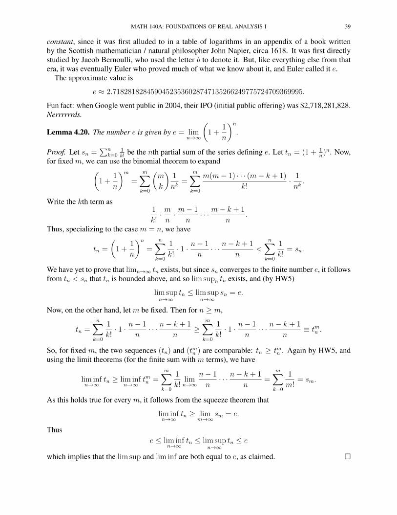
MATH 140A: FOUNDATIONS OF REAL ANALYSIS I 39
constant, since it was first alluded to in a table of logarithms in an appendix of a book writtenby the Scottish mathematician / natural philosopher John Napier, circa 1618. It was first directlystudied by Jacob Bernoulli, who used the letter b to denote it. But, like everything else from thatera, it was eventually Euler who proved much of what we know about it, and Euler called it e.
The approximate value is
e ≈ 2.71828182845904523536028747135266249775724709369995.
Fun fact: when Google went public in 2004, their IPO (initial public offering) was $2,718,281,828.Nerrrrrrds.
Lemma 4.20. The number e is given by e = limn→∞
(1 +
1
n
)n.
Proof. Let sn =∑n
k=01k!
be the nth partial sum of the series defining e. Let tn = (1 + 1n)n. Now,
for fixed m, we can use the binomial theorem to expand(1 +
1
n
)m=
m∑k=0
(m
k
)1
nk=
m∑k=0
m(m− 1) · · · (m− k + 1)
k!· 1nk.
Write the kth term as1
k!· mn· m− 1
n· · · m− k + 1
n.
Thus, specializing to the case m = n, we have
tn =
(1 +
1
n
)n=
n∑k=0
1
k!· 1 · n− 1
n· · · n− k + 1
n<
n∑k=0
1
k!= sn.
We have yet to prove that limn→∞ tn exists, but since sn converges to the finite number e, it followsfrom tn < sn that tn is bounded above, and so lim supn tn exists, and (by HW5)
lim supn→∞
tn ≤ lim supn→∞
sn = e.
Now, on the other hand, let m be fixed. Then for n ≥ m,
tn =n∑k=0
1
k!· 1 · n− 1
n· · · n− k + 1
n≥
m∑k=0
1
k!· 1 · n− 1
n· · · n− k + 1
n≡ tmn .
So, for fixed m, the two sequences (tn) and (tmn ) are comparable: tn ≥ tmn . Again by HW5, andusing the limit theorems (for the finite sum with m terms), we have
lim infn→∞
tn ≥ lim infn→∞
tmn =m∑k=0
1
k!limn→∞
n− 1
n· · · n− k + 1
n=
m∑k=0
1
m!= sm.
As this holds true for every m, it follows from the squeeze theorem that
lim infn→∞
tn ≥ limm→∞
sm = e.
Thuse ≤ lim inf
n→∞tn ≤ lim sup
n→∞tn ≤ e
which implies that the lim sup and lim inf are both equal to e, as claimed. �

40 TODD KEMP
The second form of e, as a limit, is (one of the) reason(s) it is so important: this shows thate shows up in many problems related to compound interest or exponential decay. However, as ameans of approximating e, this limit is very slow: for example
t10 ≈ 2.5937 (4.6% error), t100 ≈ 2.7048 (0.50% error).
That is: you need 100 terms in order to get 2 digits of accuracy. On the other hand, s10 is within10−8 of e, and s100 is so close to e my computer cannot compute the difference. But we can give abound on this tiny error as follows. First note that sn is increasing, so |e− sn| = e− sn. Now
e− sn =∞∑k=0
1
k!−
n∑k=0
1
k!=
∞∑k=n+1
1
k!.
Now, we factor the terms (all of which have k ≥ n+ 1) as1
k!=
1
(n+ 1)!(n+ 2)(n+ 3) · · · k=
1
(n+ 1)!· 1
(n+ 2)(n+ 3) · · · k<
1
(n+ 1)!· 1
(n+ 1)k−n−1.
Thus
e− sn <1
(n+ 1)!
∞∑k=n+1
1
(n+ 1)k−n−1=
1
(n+ 1)!
∞∑j=0
1
(n+ 1)j.
This is a geometric series, and 0 < 1n+1
< 1, so we know the sum is∞∑j=0
1
(n+ 1)j=
1
1− 1n+1
=n+ 1
n.
Thus, we have our estimate:
e− sn <1
(n+ 1)!
n+ 1
n=
1
n! · n.
This is a tiny number. Since 10! = 3, 628, 800, this shows that e − s10 < 13×107 (and in fact it’s 3
times smaller than this). For n = 100, we have 100! · 100 ≈ 10160, so s100 differs from e only afterthe 160th decimal digit!
This is one of the rare occasions where a perfectly practical question of error approximationactually allows us to prove something entirely theoretical.
Proposition 4.21. The number e is irrational.
Proof. For a contradiction, let us suppose e ∈ Q. Since e > 0, this means there are positiveintegers m,n so that e = m
n. Now, from the above estimate, we have
0 < e− sn <1
n! · n, ∴ 0 < n!e− n!sn <
1
n.
Now,
n!sn = n!n∑k=0
1
k!=
n∑k=0
n!
k!=
n∑k=0
n(n− 1) · · · (n− k + 1) ∈ N.
Also, by assumption e = mn
, and so n!e = m · (n − 1)! ∈ N. Thus ` = n!e − n!sn ∈ N. But thismeans 0 < ` < 1
nfor some n ∈ N, and that is a contradiction (there are no integers between 0 and
1n
). �
Moving to our final topic on the subject of series, let us consider absolute convergence.
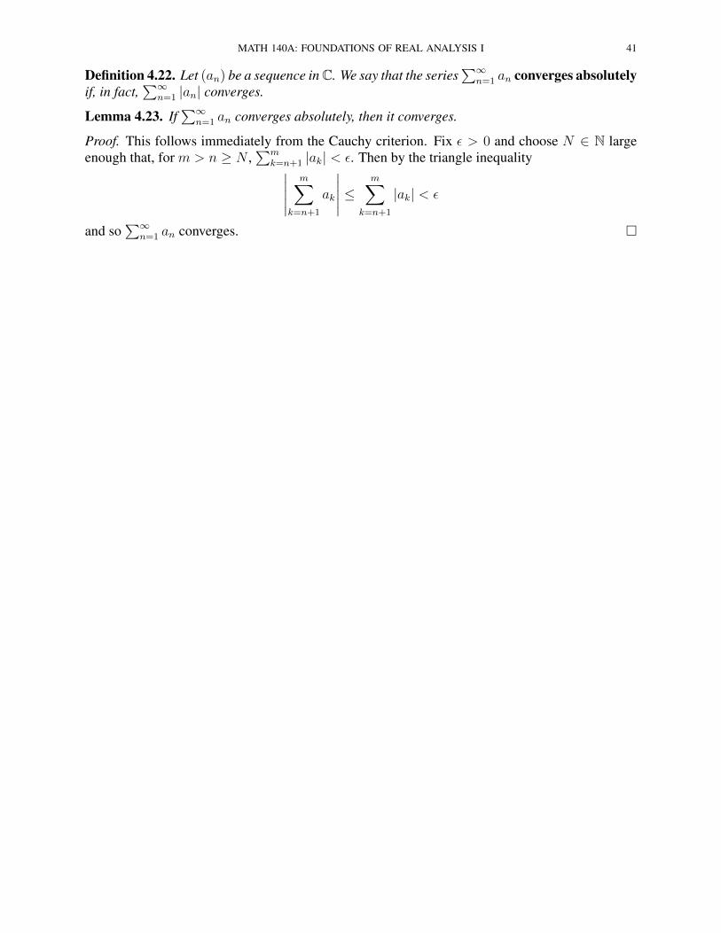
MATH 140A: FOUNDATIONS OF REAL ANALYSIS I 41
Definition 4.22. Let (an) be a sequence in C. We say that the series∑∞
n=1 an converges absolutelyif, in fact,
∑∞n=1 |an| converges.
Lemma 4.23. If∑∞
n=1 an converges absolutely, then it converges.
Proof. This follows immediately from the Cauchy criterion. Fix ε > 0 and choose N ∈ N largeenough that, for m > n ≥ N ,
∑mk=n+1 |ak| < ε. Then by the triangle inequality∣∣∣∣∣
m∑k=n+1
ak
∣∣∣∣∣ ≤m∑
k=n+1
|ak| < ε
and so∑∞
n=1 an converges. �
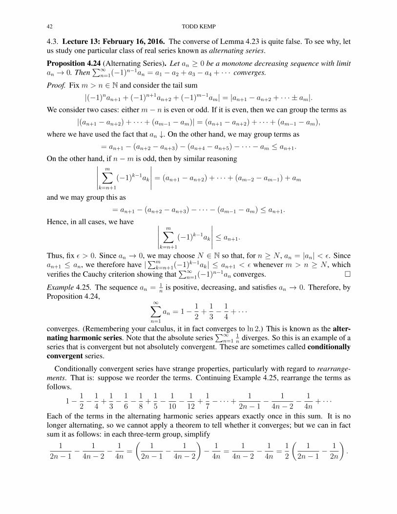
42 TODD KEMP
4.3. Lecture 13: February 16, 2016. The converse of Lemma 4.23 is quite false. To see why, letus study one particular class of real series known as alternating series.
Proposition 4.24 (Alternating Series). Let an ≥ 0 be a monotone decreasing sequence with limitan → 0. Then
∑∞n=1(−1)n−1an = a1 − a2 + a3 − a4 + · · · converges.
Proof. Fix m > n ∈ N and consider the tail sum
|(−1)nan+1 + (−1)n+1an+2 + (−1)m−1am| = |an+1 − an+2 + · · · ± am|.We consider two cases: either m− n is even or odd. If it is even, then we can group the terms as
|(an+1 − an+2) + · · ·+ (am−1 − am)| = (an+1 − an+2) + · · ·+ (am−1 − am),where we have used the fact that an ↓. On the other hand, we may group terms as
= an+1 − (an+2 − an+3)− (an+4 − an+5)− · · · − am ≤ an+1.
On the other hand, if n−m is odd, then by similar reasoning∣∣∣∣∣m∑
k=n+1
(−1)k−1ak
∣∣∣∣∣ = (an+1 − an+2) + · · ·+ (am−2 − am−1) + am
and we may group this as
= an+1 − (an+2 − an+3)− · · · − (am−1 − am) ≤ an+1.
Hence, in all cases, we have ∣∣∣∣∣m∑
k=n+1
(−1)k−1ak
∣∣∣∣∣ ≤ an+1.
Thus, fix ε > 0. Since an → 0, we may choose N ∈ N so that, for n ≥ N , an = |an| < ε. Sincean+1 ≤ an, we therefore have |
∑mk=n+1(−1)k−1ak| ≤ an+1 < ε whenever m > n ≥ N , which
verifies the Cauchy criterion showing that∑∞
n=1(−1)n−1an converges. �
Example 4.25. The sequence an = 1n
is positive, decreasing, and satisfies an → 0. Therefore, byProposition 4.24,
∞∑n=1
an = 1− 1
2+
1
3− 1
4+ · · ·
converges. (Remembering your calculus, it in fact converges to ln 2.) This is known as the alter-nating harmonic series. Note that the absolute series
∑∞n=1
1n
diverges. So this is an example of aseries that is convergent but not absolutely convergent. These are sometimes called conditionallyconvergent series.
Conditionally convergent series have strange properties, particularly with regard to rearrange-ments. That is: suppose we reorder the terms. Continuing Example 4.25, rearrange the terms asfollows.
1− 1
2− 1
4+
1
3− 1
6− 1
8+
1
5− 1
10− 1
12+
1
7− · · ·+ 1
2n− 1− 1
4n− 2− 1
4n+ · · ·
Each of the terms in the alternating harmonic series appears exactly once in this sum. It is nolonger alternating, so we cannot apply a theorem to tell whether it converges; but we can in factsum it as follows: in each three-term group, simplify
1
2n− 1− 1
4n− 2− 1
4n=
(1
2n− 1− 1
4n− 2
)− 1
4n=
1
4n− 2− 1
4n=
1
2
(1
2n− 1− 1
2n
).
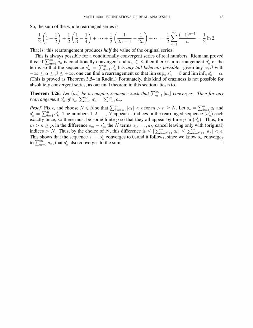
MATH 140A: FOUNDATIONS OF REAL ANALYSIS I 43
So, the sum of the whole rearranged series is
1
2
(1− 1
2
)+
1
2
(1
3− 1
4
)+ · · ·+ 1
2
(1
2n− 1− 1
2n
)+ · · · = 1
2
∞∑n=1
(−1)n−1
n=
1
2ln 2.
That is: this rearrangement produces half the value of the original series!This is always possible for a conditionally convergent series of real numbers. Riemann proved
this: if∑∞
n=1 an is conditionally convergent and an ∈ R, then there is a rearrangement a′n of theterms so that the sequence s′n =
∑nk=1 a
′n has any tail behavior possible: given any α, β with
−∞ ≤ α ≤ β ≤ +∞, one can find a rearrangement so that lim supn s′n = β and lim infn s
′n = α.
(This is proved as Theorem 3.54 in Rudin.) Fortunately, this kind of craziness is not possible forabsolutely convergent series, as our final theorem in this section attests to.
Theorem 4.26. Let (an) be a complex sequence such that∑∞
n=1 |an| converges. Then for anyrearrangement a′n of an,
∑∞n=1 a
′n =
∑∞n=1 an.
Proof. Fix ε, and choose N ∈ N so that∑m
k=n=1 |ak| < ε for m > n ≥ N . Let sn =∑n
k=1 ak ands′n =
∑nk=1 a
′k. The numbers 1, 2, . . . , N appear as indices in the rearranged sequence (a′n) each
exactly once, so there must be some finite p so that they all appear by time p in (a′n). Thus, form > n ≥ p, in the difference sm − s′m the N terms a1, . . . , aN cancel leaving only with (original)indices > N . Thus, by the choice of N , this difference is ≤ |
∑mk=N+1 ak| ≤
∑mk=N+1 |ak| < ε.
This shows that the sequence sn − s′n converges to 0, and it follows, since we know sn convergesto∑∞
n=1 an, that s′n also converges to the sum. �
44 TODD KEMP
5. METRIC SPACES
For the remainder of this course, we are going to generalize the concepts we’ve worked with(notably convergence) beyond the case of R or C. The key to this generalization was alreadydiscussed in the generalization from R to C: we replace the absolute value in R (defined in termsof the order relation) with the complex modulus in C. For all of the same technology to work, onlya few basic properties of the absolute value / modulus were needed: that |x| ≥ 0, that |x| = 0 onlywhen x = 0, and finally the triangle inequality |x+ y| ≤ |x|+ |y|.
This last property requires a notion of addition, and we’d like to move beyond vector spaces.The trick is that, in the notion of convergence, the absolute value / modulus only ever comes up asa means of measuring distance between two elements: |x − y|. Thinking of it this way, what dothe three key properties say?
• For any two elements x, y, the distance |x− y| is ≥ 0.• If the distance |x− y| is 0, then actually x = y.• The triangle inequality: for any three elements x, y, z, the distance |x − z| is bounded
above by |x− y|+ |y − z|. (This is really why it’s called the triangle inequality: draw theassociated picture.) Indeed, we have
|x− z| = |(x− y) + (y − z)| ≤ |x− y|+ |y − z|.
Interpreted in this light, we don’t need a notion of addition: everything can be stated purely interms of the notion of distance (in this case given by (x, y) 7→ |x− y|). We generalize thus.
Definition 5.1. LetX be a nonempty set. A function d : X×X → R is called a metric if it satisfiesthe following three properties.
(1) For any x, y ∈ X , d(x, y) = d(y, x) ≥ 0.(2) For any x, y ∈ X , if d(x, y) = 0, then x = y.(3) For any x, y, z ∈ X , d(x, z) ≤ d(x, y) + d(y, z).
The pair (X, d) is called a metric space.
Example 5.2. (1) As above, if we let dC(x, y) = |x− y|, then (C, dC) is a metric space. Samegoes for R equipped with the restriction of dC to R.
(2) More generally, fix n, and consider the set Cn of n-tuples of real numbers. Define theEuclidean norm on Cn as follows:
‖(x1, . . . , xn)‖2 =(|x1|2 + · · ·+ |xn|2
)1/2.
It is a simple but laborious exercise to verify that the Euclidean metric d2(x,y) = ‖x−y‖2is a metric on Cn. As above, the restriction to Rn is also a metric.
(3) There are many other, different metrics on Rn. The best known are the p-metrics: for1 ≤ p <∞,
‖(x1, . . . , xn)‖p = (|x1|p + · · ·+ |xn|p)1/p .
There is also the∞-norm, aka the sup norm
‖(x1, . . . , xn)‖∞ = max{|x1|, . . . , |xn|}.
As above, all of these norms yield metrics in the usual way, dp(x,y) = ‖x − y‖p. Note:the definition still makes sense when p < 1, but it no longer gives a metric: the triangle
MATH 140A: FOUNDATIONS OF REAL ANALYSIS I 45
inequality is violated. For example, taking p = 12, we have
‖(9, 1) + (16, 0)‖1/2 = ‖(25, 1)‖1/2 = (251/2 + 11/2)2 = 36
‖(9, 1)‖1/2 + ‖(16, 0)‖1/2 = (91/2 + 11/2)2 + (161/2 + 01/2)2 = 32 < 36.
(4) LetB[0, 1] consist of all bounded functions [0, 1]→ R. Then define a function du : B[0, 1]×B[0, 1]→ R by
du(f, g) = supx∈[0,1]
|f(x)− g(x)|.
This is well-defined: since f and g are bounded, the set {f(x) − g(x) : x ∈ [0, 1]} is abounded, nonempty set, so it has a sup. It is ≥ 0, and moreover if du(f, g) = 0, thenfor every x0 ∈ [0, 1], |f(x0) − g(x0)| ≤ supx∈[0,1] |f(x) − g(x)| = 0, which implies thatf(x0)− g(x0) = 0 – i.e. f = g. This verifies the first two properties of Definition 5.1. Forthe triangle inequality, we have
du(f, h) = supx∈[0,1]
|f(x)− h(x)| = supx∈[0,1]
|f(x)− g(x) + g(x)− h(x)|
≤ supx∈[0,1]
(|f(x)− g(x)|+ |g(x)− h(x)|)
≤ supx∈[0,1]
|f(x)− g(x)|+ supx∈[0,1]
|g(x)− h(x)|
= du(f, g) + du(g, h)
using the properties of sup we now know well. Thus the triangle inequality holds for duas well, and so it is a metric. Note, like the above examples, it has the form du(f, g) =‖f−g‖u for a norm ‖·‖u: a function onB[0, 1] which has the properties ‖f‖u ≥ 0 and = 0only if f = 0, and satisfies the triangle inequality ‖f + g‖u ≤ ‖f‖u + ‖g‖u. Whenever wehave a function like this defined on a vector space, it gives rise to a metric by subtraction.
(5) Not every metric is given in terms of a norm like this. For example, consider on R thefunction
d(x, y) = min{|x− y|, 1}.It is easy to verify that this satisfies properties (1) and (2) in Definition 5.1. The triangleinequality is also easy to see, by breaking into eight cases (depending whether |x − y|,|x− z|, and |y − z| are ≤ 1 or > 1); this boring proof is left to the reader.
(6) Given any nonempty set X , one can define a metric on X by the silly rule
d(x, y) =
{0, x = y
1, x 6= y.
This is known as the discrete metric. It says two points are close only if they are equal;otherwise they are far apart. It is again simple to verify this is a metric.
One important observation was made at several points in the examples: if (X, d) is a metricspace, and Y ⊆ X , then (Y, d|Y ) is a metric space – that is, the metric Y defined on all pairs(x, y) ∈ X×X , also defines a metric when restricted only to pairs in Y ×Y , as is straightforward toverify. Thus, the Euclidean metric on Cn automatically gives us a metric (also called the Euclideanmetric) on Rn. Similarly, the usual metric on R restricts to a metric on [0, 1].
Usually thinking of metric spaces using our intuition from R2 and R3, we introduce the followingnotation.
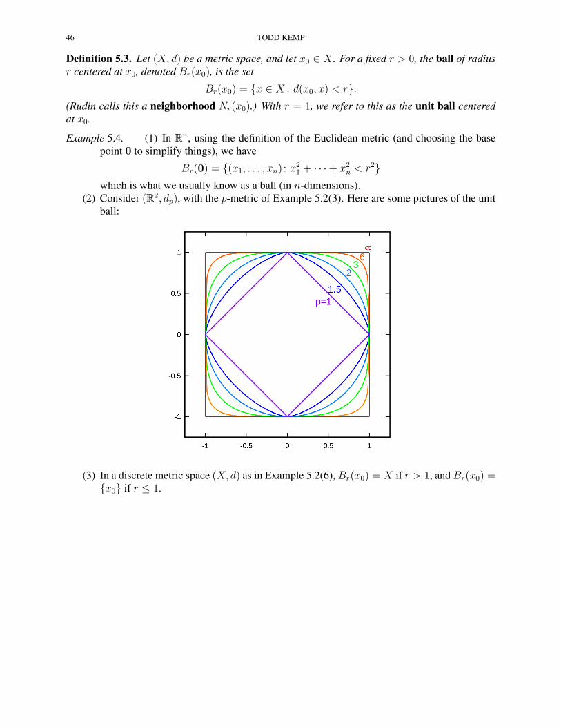
46 TODD KEMP
Definition 5.3. Let (X, d) be a metric space, and let x0 ∈ X . For a fixed r > 0, the ball of radiusr centered at x0, denoted Br(x0), is the set
Br(x0) = {x ∈ X : d(x0, x) < r}.(Rudin calls this a neighborhood Nr(x0).) With r = 1, we refer to this as the unit ball centeredat x0.
Example 5.4. (1) In Rn, using the definition of the Euclidean metric (and choosing the basepoint 0 to simplify things), we have
Br(0) = {(x1, . . . , xn) : x21 + · · ·+ x2n < r2}which is what we usually know as a ball (in n-dimensions).
(2) Consider (R2, dp), with the p-metric of Example 5.2(3). Here are some pictures of the unitball:
(3) In a discrete metric space (X, d) as in Example 5.2(6),Br(x0) = X if r > 1, andBr(x0) ={x0} if r ≤ 1.
MATH 140A: FOUNDATIONS OF REAL ANALYSIS I 47
5.1. Lecture 14: February 18, 2016. Now, once more, we define convergence and Cauchy inthe wider world of metric spaces.
Definition 5.5. Let (X, d) be a metric space, and let (xn) be a sequence in X , and let x ∈ X . Saythat (xn) converges to x, or xn → x, or limn→∞ xn = x, if
∀ε > 0 ∃N ∈ N s.t. ∀n ≥ N d(xn, x) < ε.
In other words, xn → x means that the real sequence d(xn, x) → 0. Alternatively, we could statethis as: for all sufficiently large n, xn ∈ Bε(x).
Similarly, say that (xn) is a Cauchy sequence in X if
∀ε > 0 ∃N ∈ N s.t. ∀n,m ≥ N d(xn, xm) < ε.
As discussed in the generalization from R to C, limits are unique: if xn → x and xn → y, thenx = y (this follows from the fact that d(x, y) = 0 implies that x = y; it is primarily for this reasonthat this non-degeneracy property is required in the definition of a metric).
Example 5.6. Consider a discrete metric space: (X, d) where d is given as in Example 5.2(6). Letxn → x. In particular, this means that there is some time N such that, for n ≥ N , d(xn, x) < 1
2.
But by the definition of d, either d(xn, x) = 0 or d(xn, x) = 1; so if d(xn, x) < 12
then d(xn, x) = 0,and so xn = x. Thus, if xn → x, then xn = x for all large n. In a discrete metric space,convergence is the same thing as eventually constant. The same holds true for Cauchy.
In general, there is a fundamental difference between convergent sequences that are eventuallyconstant and convergent sequences that are not eventually constant. We use this difference to defineone of the most important topological concepts.
Definition 5.7. Let (X, d) be a metric space, and let E ⊆ X be a subset. A point x ∈ X (notnecessarily in E) is called a limit point of E if there is a sequence xn ∈ E \ {x} that convergesto x, xn → x. That is: a limit point of E is a limit of some not eventually constant sequence in E.A point e ∈ E that is not a limit point of E is called an isolated point of E.
Example 5.8. In R with the usual metric, take E = (−1, 0]∪N. Then −1 is a limit point of E: forexample, −1 = lim(−1 + 1
n) and −1 + 1
n∈ E for each n. Also, any point x ∈ E is a limit point
of E: take xn = x− 1+xn
as the sequence. This is in E since 1 + x > 0 and so x− 1+xn< x ≤ 0,
but also x− 1+xn> x− (1 + x) = −1.
On the other hand, the positive integers N are isolated points of E. For example, consider 1. Ifyn is any sequence in R that converges to 1, then we must have yn ∈ (0.9, 1.1) for all large n; butthen if yn ∈ E it follows that yn = 1 for all large n, which isn’t allowed. Thus, no sequence inE \ {1} converges to 1, showing that the point 1 ∈ E is not a limit point of E – it is an isolatedpoint.
The set of all limit points of a set E is denoted E ′. So E is closed iff E ′ ⊆ E.
Definition 5.9. A subset E of a metric space is called closed if it contains all of its limit points.
Example 5.10. (1) The set E = (−1, 0] ∪ N from Example 5.8 is not closed: −1 is a limitpoint of E, but −1 6∈ E.
(2) The set F = [−1, 0] ∪ N is closed. The argument in Example 5.8 shows that each of thepoints in [−1, 0] is a limit point of F , while each of the points n ∈ N is an isolated pointof F . On the other hand, if x is a real number not in F , then either x < −1 or x > 0 andx /∈ N. In the former case, this means that no sequence in F can come within distance
48 TODD KEMP
1+x > 0 of x, and so cannot converge to x; a similar argument with x > 0 shows that x isnot a limit point of F . Thus, the set of limit points of F consists exactly of the set [−1, 0],and this set is contained in F . So F is closed.
Definition 5.9 is stated in terms of limit points to make it clear that there are two kinds ofpoints to consider in deciding whether a set is closed: isolated points and non-isolated points. Forexample, if one has a closed set, then adding to it a finite collection of isolated points will preserveclosedness. But for the purposes of a concise definition, one need not be concerned about thedistinction.
Proposition 5.11. A subset E of a metric space (X, d) is closed if and only if, for any sequence(xn) in E that converges in X , the limit limn→∞ xn is actually in E.
That is: closed means closed under limits of sequences.
Proof. Suppose E is closed, so E ′ ⊆ E. Now, let (xn) be any sequence in E that converges tosome point x. If xn 6= x for any n, then by definition x ∈ E ′, and therefore by assumption x ∈ E.If, on the other hand, there exists n with xn = x, then since xn ∈ E for each n, we have x ∈ E.Thus, the E is closed under limits of sequences.
Conversely, suppose E is closed under limits of sequences. Let x ∈ E ′; so by definition thereis a sequence xn ∈ E \ {x} such that xn → x. Well, since xn → x and xn ∈ E, by assumptionx ∈ E. Thus E ′ ⊆ E, and E is closed. �
There is a complementary notion to closed, called open.
Definition 5.12. A subset E of a metric space is called open if, for any point x ∈ E, there is a ballBr(x) (for some r > 0) with Br(x) ⊆ E.
Example 5.13. (1) The set E = (−1, 0]∪N from Example 5.8 is not open. Consider the point0 ∈ E. For any 0 < r < 1, the ball Br(0) = (−r, r) contains some points (for example r
2)
that are in (0, 1), and hence not in E. Similarly, any of the points in N are in E but none iscontained in a ball contained in E. So E is not open.
(2) On the other hand, the set U = (0, 1) is open. Indeed, let x ∈ U . Let’s consider two cases:either 0 < x < 1
2or 1
2≤ x < 1. In the former case, the ball Bx(x) = (0, 2x) is contained
in U = (0, 1); in the latter case, the ball B1−x(x) = (2x− 1, 1) is contained in U . So everypoint of x is contained in a ball inside U , showing that U is open.
(3) Let (X, d) be a discrete metric space. If x ∈ X , then by Example 5.4(3), B1(x) = {x}.Thus, every singleton point in a discrete metric space is an open set. On the other hand,by Example 5.6, there are no non-eventually-constant sequences converging to any pointx, which means every point is isolated. That is: X has no limit points, which means that(vacuously) X contains all its limit points. So X is also closed.
(4) Consider the empty set ∅ in any metric space. It is both open and closed. Indeed, thedefinitions of “open” and “closed” each start with “for every point in the set. . . ” and sincethere are no points in ∅ to check the condition, it follows that the condition holds vacuously.
Example 5.13(2) has a nice, important generalization to any metric space. Not that (0, 1) is itselfa ball in R: it is the ball B1/2(1/2). The fact is, any ball is open.
Proposition 5.14. Let (X, d) be a metric space, let x ∈ X , and let r > 0. Then the ball Br(x) isopen in X .
MATH 140A: FOUNDATIONS OF REAL ANALYSIS I 49
Proof. Let y ∈ Br(x). This means d(x, y) < r. Hence, there is some ε > 0 so that d(x, y) = r− ε.I claim that Bε(y) ⊂ Br(x). Indeed, suppose that z ∈ Bε(y), meaning that d(z, y) < ε. Then
d(x, z) ≤ d(x, y) + d(y, z) = r − ε+ d(y, z) < r − ε+ ε = r.
so z ∈ Br(x). We have thus shown that, for any y ∈ Br(x), there is a ball Bε(y) ⊂ Br(x). Thatis: Br(x) is open. �
50 TODD KEMP
5.2. Lecture 15: February 23, 2016. We referred to open and closed as complementary proper-ties. That doesn’t mean that any set is either open or closed: for example, the set (−1, 0] consideredabove is neither open nor closed. But they concepts are complementary, in the following precisesense.
Proposition 5.15. Let (X, d) be a metric space. A subset E ⊆ X is open if and only if Ec = X \Eis closed.
Since (Ec)c = E, it follows similarly that E is closed iff Ec is open. In the proof we will use thecharacterization of closed given in Proposition 5.11.
Proof. Suppose E is open. Let (xn) be a sequence in Ec that converges to some point x ∈ X . Wewant to show that x ∈ Ec; to produce a contradition, we therefore assume that x 6∈ Ec, meaningx ∈ E. Since E is open, by definition there is some r > 0 so that Br(x) ⊆ E. On the other hand,since xn → x, there is certainly some N so that d(xN , x) < r. Thus xN ∈ Br(x) ⊆ E, whichmeans that xN ∈ E. But we assumed that xN ∈ Ec, so this is a contradition. Therefore x ∈ Ec.This shows that any convergent sequence in Ec has limit in Ec, which shows that Ec is closed.
Conversely, suppose Ec is closed. Let x ∈ E. We want to show that there is some r > 0 so thatBr(x) ⊆ E; to produce a contradiction, we therefore assume that there is no such r. That meansthat, for say r = 1
n, B1/n(x) 6⊆ E, which means precisely that there is som point xn 6∈ E such that
xn ∈ B1/n(x). So, we have produced a sequence xn ∈ Ec such that d(xn, x) < 1n
, meaning thatxn → x. Thus x is the limit of a sequence in Ec, and so by assumption x ∈ Ec. This contradictsthe assumption that x ∈ E. Therefore there must be some r > 0 so that Br(x) ⊆ E, and so Ec isclosed. �
Let us make a few more definitions that pertain the local properties of open and closed sets.
Definition 5.16. Let (X, d) be a metric space, and let E ⊆ X .(1) The closure of E is the set E = E ∪ E ′.(2) A point x ∈ E is called an interior point if there is some r > 0 with Br(x) ⊆ E. The set
of all interior points of E is called the interior of E, and is denoted◦E.
(3) The boundary of E is the set ∂E = E \◦E.
Remark 5.17. Following the proof of Proposition 5.11, E can alternatively be described as the setof all limits of convergent sequences in E.
Example 5.18. Consider again the set E = (−1, 0]∪N in R, considered in Examples 5.8 and 5.10.We’ve shown that the points in (−∞,−1) and (0,∞) are not limit points (the points 1, 2, 3, . . . arein E but are isolated); on the other hand, we’ve shown that the points [−1, 0] are all limit points.Thus E ′ = [−1, 0], and so E = E ∪ E ′ = [−1, 0] ∪ N. We’ve also shown in Example 5.13(1)that there is no ball centered at 0 contained in E; similarly, there are no balls centered at the points1, 2, 3, . . . contained in E, so these are not interior points. On the other hand, an argument very
similar to Example 5.13(2) shows that the points in (−1, 0) are interior points. So◦E = (−1, 0).
Finally, this shows that ∂E = E \◦E = {−1, 0, 1, 2, . . .}.
Example 5.19. Let Q denote the rational numbers as a subset of the metric space R. By Theorem1.17(2) (the density of Q in R), given any real numbers a < b there is a rational number q ∈ Qwith a < q < b. In particular, fix x ∈ R; then for n ∈ N there is a rational number qn with
MATH 140A: FOUNDATIONS OF REAL ANALYSIS I 51
x+ 12n< qn < x+ 1
n. In particular, we have 1
2n< |qn−x| < 1
n. This shows that qn → x but qn 6= x
for any n; thus x ∈ Q′. So every real number is a limit point of Q, and so Q = Q∪Q′ = Q∪R = R.(This is another way of saying Q is dense in R; in general, we say a subset E ⊆ X is dense in ametric space X if E = X .)
On the other hand, let r > 0, and let q ∈ Q. The number x = q + r√2
is < x + r, which showsthat x ∈ (q − r, q + r) = Br(q). But x /∈ Q: indeed, we can solve
√2 = r
x−q , and so if x wererational
√2 would also be rational, which we know it is not. Thus Br(q) 6⊆ Q for any r > 0. This
shows q is not interior to Q. This holds for any q ∈ Q, and so, in fact,◦Q = ∅.
Theorem 5.20. Let (X, d) be a metric space, and let E ⊆ X .(1) E is closed; E is closed iff E = E.
(2)◦E is open; E is open iff E =
◦E.
Proof. We begin with item 1. Let (xn) be a sequence in E with limit x. We wish to show x ∈ E.If x ∈ E ⊆ E we are done, so assume x /∈ E. For each xn, either xn ∈ E or xn ∈ E ′. In the lattercase, by definition of E ′ there is some other sequence yk ∈ E such that yk → xn; in particular, wecan choose some k large enough that d(yk, xn) < 1
n. So, we can define a new sequence (x′n) as
follows: if xn ∈ E then x′n = xn; if xn 6∈ E ′, then x′n = yk as above, so x′n ∈ E and d(xn, x′n) <1n
.Then we have d(x′n, x) ≤ d(x′n, xn) + d(xn, x) <
1n+ d(xn, x) → 0, and so x′n → x. As x′n ∈ E
and x /∈ E, it follows that x is a limit point of E, and so x ∈ E ′ ⊆ E ∪ E ′ = E. Thus E is closedunder limits; by Proposition 5.11, it follows that E is closed, as claimed. Now, by definition E isclosed iff E ′ ⊆ E, and this happens iff E = E ∪ E ′ = E, proving the second point.
For item 2, let x ∈◦E; thus, there is some ball Br(x) contained in E. But by Proposition 5.14,
the ball Br(x) is open, which means all its points are interior points; thus Br(x) ⊆◦E. So, any
point in◦E is interior to
◦E, which shows that
◦E is open. By definition
◦E ⊆ E for any set E; thus
◦E = E iff E ⊆
◦E, which is the statement that every point of E is an interior point, which is
precisely the definition of E being open. �
Example 5.21. LetE ⊂ R be nonempty and bounded above. Then α = supE exists. By definition,α − 1
nis not an upper bound for E for any n ∈ N, which shows that there is an element xn ∈ E
with α − 1n< xn ≤ α. This shows that xn → α. By Remark 5.17, it follows that α ∈ E: the
supremum is always in the closure. On the other hand, if there were some r > 0 with Br(α) ⊆ E,then, for example, α + r
2∈ E. Since α + r
2> α, this contradicts α being an upper bound for E.
Thus, α is not in◦E. That is: supE ∈ E \
◦E = ∂E.

52 TODD KEMP
5.3. Lecture 16: February 25, 2016. Now we come to an important concept you may not haveencountered before: compactness.
Definition 5.22. Let (X, d) be a metric space. A subset K ⊆ X is called compact if everysequence (xn) in K has a convergent subsequence whose limit is in K.
Example 5.23. (1) Let a < b be real numbers, and consider the set K = [a, b]. The Bolzano-Weierstrass Theorem for R (Theorem 2.25) is precisely the statement that [a, b] is compact.
(2) On the other hand, E = [a, b) is not compact: the sequence xn = b − b−an
is in E, butconverges to b /∈ E, therefore all of its subsequences converge to b, and hence none ofthem converge in E. Similarly, an unbounded interval like [0,∞) is not compact: forexample the sequence xn = n has no convergent subsequences at all.
(3) Let (X, d) be a discrete metric space. IfK is a finite subset ofX , sayK = {y1, y2, . . . , ym},then K is compact. Indeed, if (xn) is any sequence in K, then there must be some (perhapsmany) yj so that xn = yj for infinitely many n (by the pigeonhole principle). That meansexactly that there is an increasing sequence nk with xnk
= yj for all k, which meansxnk→ yj ∈ K. Thus K is compact. On the other hand if E ⊆ X is infinite, it is not
compact: for then we can find an infinite sequence x1, x2, x3, . . . ∈ E all distinct. Thus,any subsequence also has all distinct terms, which means it is not eventually constant. ByExample 5.6, this means no subsequence converges.
Now, there is an alternate definition of compactness which is the only one used in Rudin; werefer to it as topological compactness, given in Definition 5.24 below. First, let us highlightthe fact that Definition 5.22 was the original definition of compact, and predated the so-called“modern” definition by almost a century. Bolzano was already using our definition of compactnessin 1817, although it would not be until 1906 that Definition 5.22 was written down formally (byFrechet). It was around this time that Lebesgue proved (as a useful lemma) that Definition 5.24 alsocharacterizes compactness; indeed, as we will see, it is a very useful tool. Much later, in 1929, theRussian school (led by Alexandrov and Urysohn) redefined compactness as what we are callingtopological compactness. Our definition of the word compact is now often called sequentiallycompact.
Definition 5.24. Let (X, d) be a metric space. Let K ⊆ X be a subset. An open cover of K is acollection (finite or infinite) of open set C in X such that every point in K is in at least on U ∈ C :that is X ⊆
⋃U . We call K topologically compact if, given any open cover C of K, there is a
finite sub cover: that is, there are finitely many U1, . . . , Um ∈ C such that K ⊆ U1 ∪ · · · ∪ Um.
Example 5.25. Consider the interval (0, 1]. We have already seen this is not compact. It is also nottopologically compact. Indeed, consider the sets Un = ( 1
n, 2) for n ∈ N. If x ∈ (0, 1) then x > 0
and so there is some n ∈ N with 1n< x. Therefore x ∈ ( 1
n, 1) ⊂ ( 1
n, 2) = Un. This shows that the
collection C = {Un : n ∈ N} is an open cover of (0, 1]. Now, consider any finite collection of setsfrom C : Un1 , Un2 , . . . , Unk
for some k ∈ N. Note that 1m< 1
`when m > `, and so U` ⊂ Um in this
case. What that means is that, if we letm = max{n1, . . . , nk} then Un1∪· · ·∪Unk= Um = ( 1
m, 2).
But then this does not cover (0, 1]: there are points x ∈ (0, 1] with x < 1m
. Thus, no finite subcoverof C will cover all of (0, 1]. The existence of such an open cover without any finite subcover showsthat (0, 1] is not topologically compact.
Theorem 5.26. Let K be a set in a subset of a metric space. Then K is sequentially compact iff Kis topologically compact.
MATH 140A: FOUNDATIONS OF REAL ANALYSIS I 53
We will not prove Theorem 5.26 here; this is the sort of thing that will be covered in an under-graduate topology course (such as Math 190). Rudin chooses to use the more abstract topologicaldefinition of compactness (for historical reasons that I find unsatisfactory), and this has the effectof both making everything more abstract, and also making all the proofs harder than necessary.We will stick exclusively with sequential compactness. This means all our proofs will be differentfrom Rudin’s – and generally shorter and easier to understand!
In Example 5.23(2), the absence of the point b from [a, b) makes the set non-compact. Note thatb is in the closure of [a, b). This highlights the following proposition.
Proposition 5.27. Compact sets are closed. Also, if K is compact and F ⊆ K is closed, then F iscompact.
Proof. Suppose K is compact. Let (xn) be a sequence in K which converges. By compactness,there is some subsequence (xnk
) that converges to a point in K. But we know that every subse-quence of (xn) converges to limxn, and hence limxn ∈ K. Thus, K is closed under limits, and soK is closed.
Now, let F be a closed subset of a compact set K. Let (yn) be any sequence in F . Then (yn)is a sequence in K, and hence by compactness there is a subsequence (ynk
) that converges in K.Note that ynk
∈ F for each k, and hence since F is closed it follows that lim ynk∈ F . Thus, any
sequence in F has a convergent subsequence with limit in F ; i.e. F is compact. �
Definition 5.28. Let E be a subset of a metric space. The diameter of E, denoted diam(E) isdefined to be
diam(E) = sup{d(x, y) : x, y ∈ E}.Note: this might well be +∞. If diam(E) < +∞, we callE bounded; otherwiseE is unbounded.
Example 5.29. (1) diam(Br(x)) ≤ 2r for any ball in a metric space. But it could be less: forexample in a discrete metric space with at least two elements, diam(Br(x)) = 0 if r ≤ 1and = 1 if r > 1.
(2) In R, diam(0, 1) = diam(0, 1] = diam[0, 1) = diam[0, 1] = 1.(3) In R, diam(N) =∞. Indeed, d(0, n) = n so sup{d(x, y) : x, y ∈ N} ≥ n for every n.
Note: if E is a bounded set, with diameter δ > 0, then for any point x ∈ E, E ⊆ B2δ(x) (orB1.0001δ(x), or Bδ+0.0001(x), etc.) Conversely, suppose there is some x in the metric space andsome r > 0 with E ⊆ Br(x). Since diam(Br(x)) ≤ 2r, it follows that diam(E) ≤ 2r. So, to sayE is bounded is the same as saying it is contained in some ball.
Proposition 5.30. Compact sets are bounded.
Proof. We prove the contrapositive: unbounded sets are not compact. Let E be unbounded, andfix a point x0 ∈ E. Consider the set of balls Bn(x0) for n ∈ N. By assumption, E 6⊆ Bn(x0) forany n, so we can choose a point xn ∈ E with d(x0, xn) ≥ n.
In fact, the sequence (xn) has no convergent subsequences. For let x be any point in the metricspace. Let n ∈ N be large enough that N > d(x0, x). Then for n ≥ N +1, we have by the triangleinequality
d(xn, x) ≥ d(xn, x0)− d(x0, x) ≥ n− d(x0, x) ≥ 1 +N − d(x0, x) > 1.
That is: for any point x in the metric space, eventually xn never comes within distance 1 of x.It follows that no subsequence of (xn) can converge to x. Since this holds for any x, it follows
54 TODD KEMP
that (xn) has no convergent subsequences. Since (xn) is a sequence in E, this means E is notcompact. �
Thus, we have seen that compact sets are closed and bounded. One of the biggest theorems ofthis course, the Heine–Borel Theorem, states that the converse is true in Euclidean space.
Theorem 5.31 (Heine–Borel). Let m ∈ N. A subset of Rm is compact iff it is closed and bounded.
Proof. Let K ⊂ Rm. If K is compact, then by Propositions 5.27 and 5.30 K is closed andbounded. We must prove the converse. Suppose K is a closed and bounded subset of Rm. Let (xn)be a sequence in K. We may write it in terms of its components
xn = (x1n, x2n, . . . , x
mn ).
Consider first the sequence (x1n)∞n=1 in R. Note that
|x1n| ≤ |xn| = d(xn, x1) ≤ diam(K).
So the sequence (x1n) is a bounded sequence in R. By Theorem 2.25 (the Bolzano-WeierstrassTheorem for R), there is a subsequence x1nk
that converges. Now we proceed as in the proof ofTheorem 3.15 (the Bolzano-Weierstrass Theorem for C). Consider the subsequence x2nk
. Againwe have |x2nk
| ≤ diam(K) is bounded, so by the Bolzano-Weierstrass Theorem for R, it possessesa further subsequence x2nk`
that is convergent. Note that x1nk`is a subsequence of the convergent
subsequence x1nk, so it is also convergent. Now we proceed to select a further convergent subsub-
subsequence that makes x3nk`sconverge, and so forth. The notation becomes ridiculous, but in the
end (after m steps) we produce a single set of indices 1 ≤ `1 < `2 < · · · such that all of thecomponents (x1`n , x
2`n, . . . , xm`n) converge as n→∞. We now follow the proof of Proposition 3.13
exactly to see that convergence in Rm is equivalent to convergence of each component separately,and so we conclude that the subsequence (x`n) converges to some element x ∈ Rm. Finally, notethat x`n ∈ K by assumption, and K is closed; thus the point x is also in K. This shows thatevery sequence in K has a convergent subsequence with limit in K, concluding the proof that Kis compact. �
MATH 140A: FOUNDATIONS OF REAL ANALYSIS I 55
5.4. Lecture 17: February 29, 2016. So, closed intervals [a, b] are compact (as we already knew),as are sets like [0, 1] ∪ [2, 3] ∪ {4, 5, 6, 7, 8}. In fact, there are much more complicated closed andbounded sets in R (e.g. the Cantor set of Example 5.34 below). Let’s emphasize that the Heine–Borel Theorem is exclusively about the metric spaces Rd; it does not apply in general.
Example 5.32. (1) Let (X, d) be a discrete metric space. Then for any two points x, y ∈ X ,either d(x, y) = 0 or d(x, y) = 1. Thus, for any subset E ⊆ X , diam(E) ≤ 1, so E isbounded. We have also shown that any subset E is closed. However, if E is an infiniteset, it is not compact, cf. Example 5.23(3). So any infinite discrete metric spaces containsclosed and bounded sets that are not compact.
(2) For a less contrived example, consider again B[0, 1], the set of all bounded, real-valuedfunctions on [0, 1], which is a metric space with respect to the metric
d(f, g) = supx∈[0,1]
|f(x)− g(x)|.
Consider the functions
fn(x) =
{1, x ≥ 1
n
0, x < 1n
.
All of these functions are in B[0, 1]. We can also compute the function fn − fm; assumingm > n we have
fm(x)− fn(x) =
0, x ≥ 1
n
1, 1m≤ x < 1
n,
0, x < 1m
.
This shows that d(fn, fm) = supx |fn(x)−fm(x)| = 1 for any m 6= n! Thus, the sequence(fn) cannot have a convergent subsequence: no two terms in the sequence are ever closerto (or farther from) each other than 1.
Here is an important property of compact sets. This is the generalization of the nested intervalsproperty that we used in the construction of R.
Proposition 5.33. Let K1, K2, K3, . . . be nonempty compact sets in a metric space, and supposethey are nested: Kn+1 ⊆ Kn for all n. Then
⋂nKn is a nonempty compact set. If, in addition,
diam(Kn)→ 0 as n→∞, then⋂nKn consists of exactly one point.
Proof. Since Kn 6= ∅ for any n, we can choose a point xn ∈ Kn for each n. By the nestedproperty, xn ∈ K1 for each n. Thus, (xn) is a sequence in the compact set K1, and therefore ithas a convergent subsequence xnk
with a limit x ∈ K1. Now, for any m ∈ N, the tail subsequence(xnk
)∞k=m also converges to x; but this is a sequence of terms in Knm , which is closed, and sox ∈ Knm . This holds for every m. Finally, for any n, there is nm > n, and therefore Knm ⊆ Kn;thus, x ∈ Kn for every n, which shows that x ∈
⋂nKn. This intersection is therefore nonempty.
It is an intersection of compact sets, therefore it is compact (Exercise 1 on HW9).For the second claim, let x, y ∈
⋂nKn. Fix ε > 0; since diam(Kn) → 0, there is some n with
diam(Kn) < ε. Thus, since x, y ∈ Kn, d(x, y) ≤ diam(Kn) < ε. So 0 ≤ d(x, y) < ε for all ε > 0;it follows that d(x, y) = 0 and so x = y. That is: there is at most one point in the intersection.As we’ve shown the intersection is nonempty, this proves that it consists of exactly one point, asclaimed. �
56 TODD KEMP
Example 5.34 (Cantor set). The unit interval K0 = [0, 1] is compact. Now remove the “middlethird” and let K1 = [0, 1
3]∪ [2
3, 1]; this set is also compact, and K1 ⊂ K0. Now repeat this: remove
the middle third from each of the two intervals inK1, producingK2 = [0, 19]∪ [2
9, 13]∪ [2
3, 79]∪ [8
9, 1].
Again, this set is compact, and K2 ⊂ K1. We can repeat this “delete middle thirds” processindefinitely. Note a certain self-similarity: K2 has two pieces, each of which looks like K1 shrunkdown by a factor of 1
3. In fact, we can inductively define
Kn =1
3Kn−1 ∪
(2
3+
1
2Kn−1
).
All of these sets are finite collections of closed, bounded intervals, so they are all compact, and theyare nested Kn+1 ⊂ Kn. Hence, by Proposition 5.33, the set C =
⋂nKn is a nonempty compact
set. This set is called the Cantor set.What can we say about this set? Well, what is the length of the longest interval in it? Note that
Kn consists of 2n intervals, each of length 13n
. Since the length of the intersection of two intervalsis≤ the length of either interval, and since C ⊂ Kn for every n, this means C contains no intervalsof length > 1
3nfor any n ∈ N; but 1
3n→ 0 as n → ∞, and therefore C contains no intervals of
length > 0. This proves that◦C = ∅. Indeed, if x were an interior point of C, that would mean
Br(x) ⊆ C for some r > 0; but Br(x) = (x− r, x + r) is an interval of length 2r > 0, which weknow is not contained in C. Thus no point is interior to C. At the same time, C is compact, so it
is closed. Thus C = C, and so ∂C = C \◦C = C – the Cantor set is its own boundary.
That also happens for discrete sets: if K consists entirely of isolated points, then K is closed
and◦K = ∅, so ∂K = K. But the Cantor set is the opposite of a discrete set: it contains no isolated
points, so C consists entirely of limit points, C ′ = C. To see this, fix x ∈ C; so x ∈ Kn for everyn. Now Kn is a collection of disjoint closed intervals, so there is some interval In ⊂ Kn withx ∈ In. Either x is in the interior of this interval or it is one of the endpoints; either way, thereis one endpoint xn of In with xn 6= x. Now, from the construction of C, the endpoints of all theintervals are in C, so xn ∈ C. Also, as diam(In) =
13n→ 0 and x, xn ∈ In, we have d(x, xn)→ 0.
This xn → x, but xn 6= x for any n, and xn ∈ C; this proves that x ∈ C ′. Since x was an arbitraryelement of C, this means C ⊆ C ′, and since C is closed, we have C ′ ⊆ C, so C = C ′.
MATH 140A: FOUNDATIONS OF REAL ANALYSIS I 57
6. LIMITS AND CONTINUITY
6.1. Lecture 18: March 3, 2016. We now begin to study functions. We have, of course, beenstudying functions (for example sequences, which are functions with domain N); now we willconcentrate on metric properties of functions. So we will set things up in terms of functionsbetween metric spaces.
Definition 6.1. Let X and Y be metric spaces. Let E ⊆ X , and let x0 ∈ E ′ be a limit point of E.Let L ∈ Y . Now, for any function f : E → Y , we say f(x) tends to L as x→ x0, or the limit asx→ x0 of f(x) is L, in symbols
limx→x0
f(x) = L
if: given any sequence (xn) in E \ {x0} that converges xn → x0, it follows that the sequence(f(xn)) in Y converges f(xn)→ L.
This is a more general kind of limit than the limit of a sequence: we are letting the argument“tend to” a limit point through a set that may be quite different from N. Our definition makes useof our knowledge of limits of sequences. This is useful, for example, in establishing some of thebasic properties of limits. For example:
Lemma 6.2. Limits are unique: if limx→x0 f(x) = L1 and limx→x0 f(x) = L2, then L1 = L2.
Proof. Since x0 is a limit point, there is a sequence (xn) with xn 6= x0 for any n and xn → x0. Bydefinition of limx→x0 f(x) = L1, this means that the sequence f(xn) converges to L1; by definitionof limx→x0 f(x) = L2, this means that f(xn) converges to L2. Thus, by uniqueness of limits ofsequences, L1 = L2. �
Remark 6.3. (1) If we had not included in the definition the fact that x0 is a limit point, this ar-gument would fail. Indeed, if x0 is an isolated point, vacuously it holds that limx→x0 f(x) =L for all L.
(2) On the other hand, we might try to modify the definition of limit so that this wouldn’thappen: we could, for example, insist that f(xn)→ L for any sequence xn that convergesto x0, even if it does hit x0 at some times. But this would rule out some of our intuitionabout limits, as the following example shows.
Example 6.4. Consider the function f : R→ R given by
f(x) =
{0, x 6= 0
1, x = 0.
We know from our calculus intuition that limx→0 f(x) = 0. Indeed, we can verify this fromDefinition 6.1: if xn is any sequence in R \ {0}, then f(xn) = 0 for all n, and the constantsequence 0 does indeed converge to 0.
On the other hand, suppose we had left out the xn 6= x0 clause in Definition 6.1, and insistedthat f(xn) → L for every sequence xn → x0. In this scenario, the function above would have nolimit at 0. Indeed, we could take the sequence xn = 1
nif n is even and xn = 0 if n is odd. Then
the sequence f(xn) = (0, 1, 0, 1, 0, 1, . . .) has no limit.
This illustrates the fundamental idea of limits: a limit is where a function is going as you ap-proach the limit point; it is unrelated to the actual value of the function at that point (if it is evendefined).
58 TODD KEMP
We can use our theory of limits of sequences to calculate many limits. For example, if therange space for the function is the familiar C, we have the following echo of the limit theorems forC-sequences:
Theorem 6.5 (Limit Theorems). Let f, g : X → C, and let x0 be a limit point inX . If limx→x0 f(x) =L and limx→x0 g(x) =M , then
limx→x0
[f(x) + g(x)] = L+M, and limx→x0
[f(x) · g(x)] = L ·M.
Proof. Let (xn) be any sequence in X \{x0} that converges to x0. By assumption, f(xn)→ L andg(xn)→M . Thus, by the limit theorems for sequences in C, cf. Theorem 2.27, f(xn) + g(xn)→L+M and f(xn)·g(xn)→ L·M . This is precisely what it means to say that limx→x0 [f(x)+g(x)] =L+M and limx→x0 [f(x) · g(x)] = L ·M . �
There is an equivalent definition of limit which does not explicitly rely on sequences. Thisdefinition is one of the crowning achievements of 19th Century mathematics. The calculus wasbuilt on an intuitive understanding of limits in the minds of Newton and Liebnitz (and others),but it wasn’t until Weierstrass came up with this modern definition that analysis of functions wasfinally put on rigorous footing.
Theorem 6.6. Let (X, dX) and (Y, dY ) be metric spaces, let E ⊆ X , let f : E → Y be a function,let x0 ∈ E ′, and let L ∈ Y . Then limx→x0 f(x) = L if and only if the following holds true:
∀ε > 0 ∃δ > 0 s.t. ∀x ∈ E, x ∈ Bδ(x0) \ {x0} =⇒ f(x) ∈ Bε(L).
I.e.∀ε > 0 ∃δ > 0 s.t. ∀x ∈ E, 0 < dX(x, x0) < δ =⇒ dY (f(x), L) < ε. (6.1)
In words: to say f(x) tends to L as x tends to x0 means that, for any tolerance ε > 0, no matterhow small, there is some (potentially even smaller) tolerance δ > 0 so that, if x is δ-close to x0(but not equal to x0), then f(x) is ε-close to L.
Proof. First, suppose that (6.1) holds. Let xn ∈ E \ {x0} be a sequence converging to x0. Fixε > 0, and let δ > 0 be the corresponding δ. Now, as xn → x0, there is some N ∈ N so that, forn ≥ N , dX(xn, x0) < δ. It follows from (6.1) that dY (f(xn), L) < ε for all n ≥ N . This provesthat f(xn)→ L. Thus, we have shown that limx→x0 f(x) = L by definition.
Conversely, suppose (6.1) fails to hold. This means that there exists some ε > 0 so that, for allδ > 0, there is some point xδ ∈ Bδ(x0) \ {x0} such that f(xδ) is not in Bε(L). In particular, dothis with δ = 1
n: for each n ∈ N, choose some xn ∈ B 1
n(x0) such that dY (f(xn), L) ≥ ε. On the
one hand, since 0 < dX(xn, x0) <1n→ 0, we have xn → x0 but xn 6= x0. On the other hand,
since dY (f(xn), L) ≥ ε for all n, this means that the sequence f(xn) does not converge to L. Bydefinition, this means that the statement limx→x0 f(x) = L is false. �
Example 6.7. Let us work directly from the ε–δ definition of (6.1) to show that limx→2 x2 = 4.
Here the domain and range metric spaces are both R. Fix ε > 0. We want to guarantee that|x2− 4| < ε. Write this as |x− 2||x+2| < ε. We want to choose δ > 0 and force 0 < |x− 2| < δ,meaning 2 − δ < x < 2 + δ. So, as long as we assure that δ ≤ 2, this means that 0 ≤ x ≤ 4, inwhich case |x− 2||x+ 2| ≤ 6|x− 2|. Thus, it suffices to make sure that 6|x− 2| < ε, which is tosay |x− 2| < ε/6. This tells us how to choose δ.

MATH 140A: FOUNDATIONS OF REAL ANALYSIS I 59
So, starting fresh: Let ε > 0. Choose δ = ε/6 if this is < 2, or δ = 2 otherwise. Then, so longas 0 < |x− 2| < δ, we have 0 ≤ 2− δ < x < 2 + δ ≤ 4, and so
|x2 − 4| = |x+ 2||x− 2| ≤ 6|x− 2| < 6 · ε6= ε.
Thus, by (6.1), we have proven that limx→2 x2 = 4.
On the other hand, if we refer to Theorem 6.5, we see that this follows from the fact thatlimx→2 x = 2 (which is easy to verify by either definition of limit) and therefore limx→2 x · x =2 · 2 = 4. Similar considerations show that limx→x0 f(x) = f(x0) holds for any point x0 ∈ R (orC) if f is a polynomial, for example.
60 TODD KEMP
6.2. Lecture 19: March 8, 2016. In Example 6.7, what we showed is that the function f(x) = x2
satisfies limx→2 f(x) = f(2). We should recognize this as saying that f is continuous at 2.
Definition 6.8. Let X, Y be metric spaces, E ⊆ X , and f : E → Y . Let x0 ∈ E ′ be a limit point.Say that f is continuous at x0 if
limx→x0
f(x) = f(x0).
Note that this only defines continuity at limit points: we have left undefined what it would mean forf to be continuous at an isolated point of its domain of definition. Indeed, what should we meanby saying that a function is continuous on the set N? This is, to some degree, up to debate. Thestandard answer is to say this is a vacuous condition: every function is continuous on a discrete set.
Now, consider again Example 6.7. To use the definition of limit, we assumed that d(x, x0) =|x − 2| > 0 (as limits are about where you’re going, not where you get to). However, observethat this requirement was never used in the proof. That is generically true in limits of continuousfunctions, as the next result demonstrates.
Proposition 6.9. Let X, Y be metric spaces and f : X → Y . Let x0 ∈ X ′. Then f is con-tinuous at x0 if and only if for every sequence (xn) in X with limn→∞ xn = x0, it follows thatlimn→∞ f(xn) = f(x0). Similarly, f is continuous at x0 if and only if
∀ε > 0 ∃δ > 0 s.t. ∀x ∈ E, dX(x, x0) < δ =⇒ dY (f(x), f(x0)) < ε.
That is: we need not assume that the sequence (xn) never hits x0; and we need not remove x0 fromthe δ-ball in the ε–δ definition of the limit. In fact, with these assumption no longer required, thereis no reason to assume x0 ∈ X ′; this definition makes perfect sense for isolated points as well,so we take it more generally as the definition of continuity. From this more general definition, itfollows that any function is continuous at an isolated point of its domain (as you should work out).
Proof. Suppose that xn → x0 implies f(xn) → f(x0) in general; then in particular this holds ifwe also assume that xn 6= x0 for any n, which means that limx→x0 f(x) = f(x0) by definition.Thus f is continuous at x0. Conversely (in contrapositive form), suppose there is some sequencexn → x0 such that f(xn) 6→ f(x0). This means there is some ε > 0 so that d(f(xn), f(x0)) ≥ εfor infinitely many n. So let n1, n2, n3, . . . be these infinitely many indices where, for each k,d(f(xnk
), f(x0)) ≥ ε; then (xnk)∞k=1 is a sequence in X that converges to x0 (as a subsequence of
a sequence xn which converge to x0), but f(xnk) 6→ f(x0) and, moreover, since f(xnk
) 6= f(x0)for any k, it follows that xnk
6= x0 for any k. This shows, from the definition, that it is false thatlimx→x0 f(x) = f(x0), completing the proof of the first statement.
The proof of the equivalence of the ε–δ statement is similar and left to the reader. �
The point is: when the putative limit is the value of the function at the limit point, there is noreason to exclude the limit point from consideration: where you are going and where you get toare the same in this case!
Example 6.10. Let (X, d) be a metric space, and let y ∈ X . Then the function f(x) = d(x, y) iscontinuous at every point in X . Indeed, fix x ∈ X , and let (xn) be a sequence in X with xn → x.Then
d(xn, y) ≤ d(xn, x) + d(x, y)
and so d(xn, y)− d(x, y) ≤ d(xn, x). But also
d(x, y) ≤ d(x, xn) + d(xn, y)
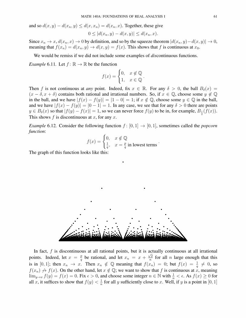
MATH 140A: FOUNDATIONS OF REAL ANALYSIS I 61
and so d(x, y)− d(xn, y) ≤ d(x, xn) = d(xn, x). Together, these give
0 ≤ |d(xn, y)− d(x, y)| ≤ d(xn, x).
Since xn → x, d(xn, x)→ 0 by definition, and so by the squeeze theorem |d(xn, y)−d(x, y)| → 0,meaning that f(xn) = d(xn, y)→ d(x, y) = f(x). This shows that f is continuous at x0.
We would be remiss if we did not include some examples of discontinuous functions.
Example 6.11. Let f : R→ R be the function
f(x) =
{0, x 6∈ Q1, x ∈ Q
.
Then f is not continuous at any point. Indeed, fix x ∈ R. For any δ > 0, the ball Bδ(x) =(x − δ, x + δ) contains both rational and irrational numbers. So, if x ∈ Q, choose some y 6∈ Qin the ball, and we have |f(x) − f(y)| = |1 − 0| = 1; if x /∈ Q, choose some y ∈ Q in the ball,and we have |f(x) − f(y)| = |0 − 1| = 1. In any case, we see that for any δ > 0 there are pointsy ∈ Bδ(x) so that |f(y)− f(x)| = 1, so we can never force f(y) to be in, for example, B 1
2(f(x)).
This shows f is discontinuous at x, for any x.
Example 6.12. Consider the following function f : [0, 1] → [0, 1], sometimes called the popcornfunction:
f(x) =
{0, x /∈ Q1q, x = p
qin lowest terms
.
The graph of this function looks like this:
In fact, f is discontinuous at all rational points, but it is actually continuous at all irrationalpoints. Indeed, let x = p
qbe rational, and let xn = x +
√2n
for all n large enough that thisis in [0, 1]; then xn → x. Then xn /∈ Q meaning that f(xn) = 0; but f(x) = 1
q6= 0, so
f(xn) 6→ f(x). On the other hand, let x /∈ Q; we want to show that f is continuous at x, meaninglimy→x f(y) = f(x) = 0. Fix ε > 0, and choose some integer n ∈ N with 1
n< ε. As f(x) ≥ 0 for
all x, it suffices to show that f(y) < 1n
for all y sufficiently close to x. Well, if y is a point in [0, 1]
62 TODD KEMP
where f(y) ≥ 1n
, then y ∈ Q and, when written in lowest terms, y = pq
with q ≤ n. There are onlyfinitely many such rational numbers, and x (which is irrational) is not one of them. Thus, we candefine δ = min{|x− y| : y = p
qin lowest terms, with q ≤ n}; then for |y − x| < δ, it follows that
f(y) < 1n< ε, proving that limy→x f(y) = 0, and so f is continuous at x.
In Examples 6.11 and 6.12, we looked at the set of points where a function is continuous. Thatis: if f : X → Y is a function and E ⊆ X , say that f is continuous on E if, for each x ∈ E, f iscontinuous at x.
Example 6.13. Let X = (0, 1), and let f : (0, 1) → R be the function f(x) = 1x. Then f is
continuous on its whole domain: for every x ∈ (0, 1), f is continuous at x. We could see thisby applying the limit theorems; but let’s use this as an opportunity to practice our ε–δ proofs. Fixε > 0. We want to guarantee that, when y is close to x, we have | 1
x− 1
y| < ε. That is
1
x− ε < 1
y<
1
x+ ε.
We only need this to hold for all sufficiently small ε > 0, so it’s fine to assume ε is small enoughthat 1
x− ε > 0. Thus we can reciprocate to get
1
1/x− ε> y >
1
1/x+ ε.
Now, subtract x from both sides and we have−εx
1/x+ ε=
1
1/x+ ε− x < y − x < 1
1/x− ε− x =
εx
1/x− ε.
This shows us how to choose δ: we define
δ = min
{εx
1/x+ ε,
εx
1/x− ε
}=
εx
1/x+ ε. (6.2)
Then, reversing the above steps, we have that for any y ∈ Bδ(x), we have |y−x| < εx1/x+ε
< εx1/x−ε ,
and this gives in particular the above two inequalities that can be reversed to say | 1x− 1
y| < ε. So
we have proved that there is a δ > 0 for any given ε > 0 (as long as ε < 1x; otherwise, if ε ≥ 1
x≥ 1,
we could take δ to be something silly and big), proving continuity at x.

MATH 140A: FOUNDATIONS OF REAL ANALYSIS I 63
6.3. Lecture 20: March 10, 2016. In Example 6.13, we showed explicitly that the functionf(x) = 1
xis continuous at every point x ∈ (0, 1). But note: the δ we had to choose for each
ε > 0 in (6.2) depends on x as well as ε. This will generically be true. Look at the ε–δ definitionof continuity: a function f is continuous on a set E if
∀x ∈ E ∀ε > 0 ∃δ > 0 s.t. ∀y ∈ E, dX(x, y) < δ =⇒ dY (f(x), f(y)) < ε. (6.3)
Having chosen a x and ε > 0, we must then find a suitable δ = δ(x, ε). In Example 6.13, not onlydoes δ depend on x, but it does so in a bad way: as x→ 0, for given ε > 0, the δ → 0 as well (quitefast, in fact: the numerator is shrinking and the denominator is growing). The closer x is to 0, thesmaller δ must be to get the same control over the function. So, while the function is continuous,there is a lack of uniformity in how continuous it is. (Note: we have shown this δ works; one mightask whether a larger, possibly more uniform δ could work just as well. The answer is no: it is nothard to show in this example that the δ in (6.2) is the largest possible δ for the given x and ε; it iscalled the modulus of continuity of the function.)
Definition 6.14. Let X, Y be metric spaces, E ⊆ X , and f : E → Y . Call f uniformly continu-ous on E if
∀ε > 0 ∃δ > 0 s.t. ∀x, y ∈ E, dX(x, y) < δ =⇒ dY (f(x), f(y)) < ε. (6.4)
Compare (6.4) with (6.3). The difference appears subtle: just the placement of the quantifier ∀x.This makes a world of difference: (6.4) says that, not only is f continuous at each point x, but onecan choose a δ = δ(ε) that is uniform: it need not depend on x. This outlaws behavior like thefunction f(x) = 1
xnear 0.
Example 6.15. Let f(x) = 2x on R. Then |f(x) − f(y)| = 2|x − y|, so for any ε > 0, we maylet δ = ε/2; then if |x − y| < δ = ε/2, it follows that |f(x) − f(y)| = 2|x − y| < 2δ = ε. Thisshows that f is continuous at all points; moreover, we may choose δ = δ(ε) = ε/2 uniformly overall x, y ∈ R. Thus, f is uniformly continuous on R.
Example 6.16. Let f(x) = x2 on [0,∞). We want to make |x2 − y2| small. We have |x2 − y2| =(x+y)|x−y|. Thus, in order for |x2−y2| < ε, we must have |x−y| < ε
x+y(these are equivalent).
But this shows that f is not uniformly continuous. Indeed, in order for |x − y| < δ to imply that|x− y| < ε
x+y, we must have δ ≤ ε
x+y; and there is no positive number δ = δ(ε) that is ≤ ε
x+yfor
all x, y > 0.
In Examples 6.13 and 6.16, we saw continuous functions on the intervals (0, 1) and [0,∞) thatare not uniformly continuous. In both cases, the non-uniformity was manifest by uncontrolledgrowth near the “edge”. As it turns out, if the domain of the continuous function is compact, thiscannot happen. That will be our final big theorem of this class.
Theorem 6.17. Let X, Y be metric spaces, K ⊆ X compact, and f : K → Y a continuousfunction. Then f is uniformly continuous.
Proof. Suppose, for a contradiction, that f is not uniformly continuous on K. Negating Definition6.14, this means
∃ε > 0 ∀δ > 0 ∃x, y ∈ K s.t. dX(x, y) < δ, but dY (f(x), f(y)) ≥ ε.
That is: there is a positive number ε > 0 so that, for every positive number δ > 0, we can findtwo points x and y that are within distance δ of each other, but such that f(x) and f(y) are at
64 TODD KEMP
least ε apart. So, let’s do this with δ = 1n
for any given positive integer: we can find xn, yn withdX(xn, yn) <
1n
, and yet dY (f(xn), f(yn)) ≥ ε.Now, we use the compactness of the domainK: the sequence (xn) has a convergent subsequence
(xnk) with a limit x ∈ K. Consider, now, the corresponding subsequence ynk
; this has a convergentsubsequence ynk`
with a limit y ∈ K. Now, xnk`is a subsequence of xnk
which converges to x,hence xnk`
→ x as well. But we also have
dX(xnk`, ynk`
) <1
nk`<
1
`→ 0.
Hence, it follows from the triangle inequality that x = y. On the other hand, by their very con-struction, the points xnk`
and ynk`all satisfy
dY (f(xnk`), f(ynk`
)) ≥ ε. (6.5)
But xnk`→ x and so, since f is continuous, f(xnk`
) → f(x); similarly, ynk`→ y = x, and so by
continuity f(ynk`)→ f(y) = f(x). Thus, by Problem 4 on Exam 2,
dY (f(xnk`), f(ynk`
))→ dY (f(x), f(x)) = 0.
This contradicts (6.5). Thus, we have proven that f is, in fact, uniformly continuous. �
Theorem 6.17 is typically the best way to prove uniform continuity of a function. For example:any polynomial is continuous on R, but, as we saw in Example 6.16, they need not be uniformlycontinuous. By Theorem 6.17, polynomial functions on compact intervals [a, b] are automaticallyuniformly continuous. What’s more: once you know a function is uniformly continuous on a setK, it is then automatically uniformly continuous on any subset E ⊆ K (the same δ = δ(ε) thatworks on all of K also works on all of E ⊆ K). So, for example, polynomials are uniformlycontinuous on all bounded intervals (a, b), (a, b], etc. Similarly, the function f(x) = 1
xof Example
6.13 is uniformly continuous on [α, 1] for any α > 0. We could see this directly from (6.2), sincethe modulus of continuity
δ = δ(x, ε) =εx
1/x+ ε
decreases as x decreases; it follows that the uniform δ = δ(α, ε) will work for all x ≥ α. However,this gets smaller as α shrinks, and if we include all of (0, 1] in the domain, there is no uniform δ.For an alternate proof of the non-uniformity in this example, see HW10.4.
Here is another very useful property of continuous functions on compact sets.
Proposition 6.18. LetX, Y be metric spaces,K ⊆ X compact, and f : K → Y continuous (henceuniformly continuous). Then the image f(K) ⊆ Y is compact.
To be clear: f(K) denotes the image of f on K:
f(K) = {f(x) ∈ Y : x ∈ K} = {y ∈ Y : ∃x ∈ K s.t. y = f(x)}.
Proof. Let (yn) be any sequence in f(K). By definition of f(K), for each yn, there exists some(or potentially many) xn ∈ K such that yn = f(xn). Since K is compact, it then follows that thesequence (xn) has a convergent subsequence (xnk
) with limit x ∈ K. Since f is continuous, itthen follows that f(xnk
)→ f(x) as k →∞. Since x ∈ K, f(x) ∈ f(K). Thus, the subsequenceynk
= f(xnk) of yn = f(xn) converges in K. We have thus shown that every sequence in f(K)
has a convergent subsequence with limit in f(K); that is, f(K) is compact. �
MATH 140A: FOUNDATIONS OF REAL ANALYSIS I 65
Corollary 6.19 (Minimax Theorem). LetK be a nonempty compact metric space, and f : K → R.Then f attains its maximum and minimum values on K.
Corollary 6.19 is a standard result stated in calculus classes, usually in the special case thatK = [a, b] is a compact interval in R.
Proof. By Proposition 6.18, f(K) is compact. In particular, it is closed and bounded. It is alsononempty since K is nonempty (so f(K) contains f(x) for any x ∈ K). Thus, by the least upperbound property of R, the set f(K) ⊂ R has a supremum M and and infimum m. Now, for anyn ∈ N, M − 1
n< M , which means that M − 1
nis not an upper bound for f(K); thus, there is some
yn ∈ f(K) with M − 1n< yn ≤ M Hence, by the Squeeze Theorem, yn → M . By definition
of f(K), there exists some xn ∈ K with yn = f(xn). Since K is compact, there is a convergentsubsequence (xnk
) of (xn), with limit x ∈ K. Since f is continuous, ynk= f(xnk
) → f(x).But ynk
is a subsequence of yn which converges to M ; thus f(x) = M . We have thereforefound a x ∈ K for which f(x) = M = sup f(K). That is: sup f(K) = max f(K), and themaximum is achieved at the point x. A very similar argument shows there is a point x′ withf(x′) = m = inf f(K), completing the proof. �