material requirementsplanning mrp - anadolu … · 5/8/2013 1 material requirementsplanning ‐mrp...
TRANSCRIPT

5/8/2013
1
Material Requirements Planning ‐MRP
ENM308Production Planning and Control ‐ I
Spring 2013Haluk Yapıcıoğlu, PhD
Aggregate Planning
Master Production Schedule
Inventory Control
Operations Scheduling
Vehicle Routing
Forecast of Demand
Hierarchy of Production Decisions

5/8/2013
2
Hierarchy of Production Decisions
• Forecasting: First, a firm must forecast demand for aggregate sales over the planning horizon.
• Aggregate planning: The forecasts provide inputs for determining aggregate production and workforce levels over the planning horizon.
• Master production schedule (MPS): Recall, that the aggregate production plan does not consider any “real” product but a “fictitious” aggregate product. The MPS translates the aggregate plan output in terms of specific production goals by product and time period.
Hierarchy of Production Decisions
• Suppose that a firm produces three types of chairs: ladder‐back chair, kitchen chair and desk chair. The aggregate production considers a fictitious aggregate unit of chair and find that the firm should produce 550 units of chairs in April. The MPS then translates this output in terms of three product types and four work‐weeks in April. The MPS suggests that the firm produce 200 units of desk chairs in Week 1, 150 units of ladder‐back chair in Week 2, and 200 units of kitchen chairs in Week 3.
• Material Requirements Planning (MRP): A product is manufactured from some components or subassemblies. For example a chair may require two back legs, two front legs, 4 leg supports, etc.

5/8/2013
3
Hierarchy of Production DecisionsMaster Production Schedule
Ladder‐back chair
Kitchen chair
Desk chair
1 2
April May
790
3 4 5 6 7 8
200
150
120
200
150
200
120
Aggregate production plan for chair family
550
200
Hierarchy of Production Decisions
• While forecasting, aggregate plan and MPS consider the volume of finished products, MRP plans for the components, and subassemblies. A firm may obtain the components by in‐house production or purchasing. MRP prepares a plan of in‐house production or purchasing requirements of components and subassemblies.
• Scheduling: Scheduling allocates resource over times in order to produce the products. The resources include workers, machines and tools.
• Vehicle Routing: After the products are produced, the firm may deliver the products to some other manufacturers, or warehouses. The vehicle routing allocates vehicles and prepares a route for each vehicle.

5/8/2013
4
Hierarchy of Production Decisions:Materials Requirement Planning
Back slats
Leg supports
Seat cushion
Seat‐frameboards
Frontlegs
Backlegs
Material Requirements Planning
• The demands for the finished goods are obtained from forecasting. These demands are called independent demand.
• The demands for the components or subassemblies depend on those for the finished goods. These demands are called dependent demand.
• Material Requirements Planning (MRP) is used for dependent demand and for both assembly and manufacturing
• If the finished product is composed of many components, MRP can be used to optimize the inventory costs.

5/8/2013
5
Inventory without an MRP System
Inventory with an MRP System
Importance of an MRP System
Importance of an MRP System
• Without an MRP system:– Component is ordered at time A, when the inventory level of the component hits reorder point, R
– So, the component is received at time B. – However, the component is actually needed at time C, not B. So, the inventory holding cost incurred between time B and C is a wastage.
• With an MRP system:– We shall see that given the production schedule of the finished goods and some other information, it is possible to predict the exact time, C when the component will be required. Order is placed carefully so that it is received at time C.

5/8/2013
6
MRP Input and Output
• MRP Inputs:
– Master Production Schedule (MPS): The MPS of the finished product provides information on the net requirement of the finished product over time.
– Inventory file: For each item, the number of units on hand is obtained from the inventory file.
MRP Input and Output
• MRP Inputs:– Bill of Materials: For each component, the bill of materials provides information on the number of units required, source of the component (purchase/ manufacture), etc. There are two forms of the bill of materials:
• Product Structure Tree: The finished product is shown at the top, at level 0. The components assembled to produce the finished product is shown at level 1 or below. The sub‐components used to produce the components at level 1 is shown at level 2 or below, and so on. The number in the parentheses shows the requirement of the item. For example, “G(4)” implies that 4 units of G is required to produce 1 unit of B.
• For each item, the name, number, source, and lead time of every component required is shown on the bill of materials in a tabular form.

5/8/2013
7
MRP Input and Output
• MRP Output:
– Every required item is either produced or purchased. So, the report is sent to production or purchasing.
MRPcomputerprogram
Bill ofMaterials
file
Inventoryfile
Master Production Schedule
ReportsTo Production
To Purchasing
ForecastsOrders
MRP Input and Output

5/8/2013
8
Level 1
Level 0
Level 2
Level 3
Bill of Materials: Product Structure Tree
BILL OF MATERIALSProduct Description: Ladder‐back chairItem: AComponent Quantity
RequiredSource
Item DescriptionB Ladder‐back 1 ManufacturingC Front legs 2 PurchaseD Leg supports 4 PurchaseE Seat 1 Manufacturing
Bill of Materials

5/8/2013
9
BILL OF MATERIALSProduct Description: SeatItem: EComponent Quantity
RequiredSource
Item DescriptionH Seat frame 1 ManufacturingI Seat cushion 1 Purchase
Bill of Materials
On Hand Inventory and Lead time
Component Units in Inventory
Lead Time (weeks)
Seat aubassembly 25 2
Seat Frame 50 3
Seat Frame Boards 75 1

5/8/2013
10
MRP Calculation
• Suppose that 150 units of ladder‐back chair is required.• The previous slide shows a product structure tree with seat
subassembly, seat frames, and seat frame boards. For each of the above components, the previous slide also shows the number of units on hand.
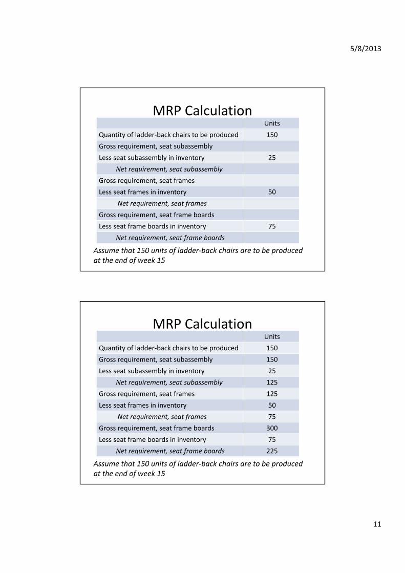
• The net requirement is computed from top to bottom. Since 150 units of ladder‐back chair is required, and since 1 unit of seat subassembly is required for each unit of ladder‐back chair, the gross requirement of seat‐subassembly is 150x1 =150 units. Since there are 25 units of seat‐subassembly in the inventory, the net requirement of the seat‐subassembly is 150 – 25 = 125 units.
MRP Calculation
• Since 1 unit of seat frames is required for each unit of seat subassembly, the gross requirement of the seat frames is 1251 = 125 units. (Note that although it follows from the product structure tree that 1 unit of seat frames is required for each unit of ladder‐back chair, the gross requirement of seat frames is not 150 units because each of the 25 units of seat‐subassembly also contains 1 unit of seat frames.) Since there are 50 units of seat frames in the inventory, the net requirement of the seat frames is 125‐50 = 75 units. The detail computation is shown in the next two slides.
• A similar logic is used to compute the time of order placement.
5/8/2013
11
Assume that 150 units of ladder‐back chairs are to be produced at the end of week 15
Units
Quantity of ladder‐back chairs to be produced 150
Gross requirement, seat subassembly
Less seat subassembly in inventory 25
Net requirement, seat subassembly
Gross requirement, seat frames
Less seat frames in inventory 50
Net requirement, seat frames
Gross requirement, seat frame boards
Less seat frame boards in inventory 75
Net requirement, seat frame boards
MRP Calculation
Assume that 150 units of ladder‐back chairs are to be produced at the end of week 15
Units
Quantity of ladder‐back chairs to be produced 150
Gross requirement, seat subassembly 150
Less seat subassembly in inventory 25
Net requirement, seat subassembly 125
Gross requirement, seat frames 125
Less seat frames in inventory 50
Net requirement, seat frames 75
Gross requirement, seat frame boards 300
Less seat frame boards in inventory 75
Net requirement, seat frame boards 225
MRP Calculation

5/8/2013
12
Assume that 150 units of ladder‐back chairs are to be produced at the end of week 15 and that there is a one‐week lead time for ladder‐back chair assembly
Week
Complete order for seat subassembly 14
Minus lead time for seat subassembly 2
Place an order for seat subassembly
Complete order for seat frames
Minus lead time for seat frames 3
Place an order for seat frames
Complete order for seat frame boards
Minus lead time for seat frame boards 1
Place an order for seat frame boards
MRP Calculation: Time of Order Placement
Assume that 150 units of ladder‐back chairs are to be produced at the end of week 15 and that there is a one‐week lead time for ladder‐back chair assembly
Week
Complete order for seat subassembly 14
Minus lead time for seat subassembly 2
Place an order for seat subassembly 12
Complete order for seat frames 12
Minus lead time for seat frames 3
Place an order for seat frames 9
Complete order for seat frame boards 9
Minus lead time for seat frame boards 1
Place an order for seat frame boards 8
MRP Calculation: Time of Order Placement

5/8/2013
13
MRP Calculation: Some Definitions
• Scheduled Receipts: – Items ordered prior to the current planning period and/or
– Items returned from the customer
• Lot‐for‐lot (L4L)– Order quantity equals the net requirement
– Sometimes, lot‐for‐lot policy cannot be used. There may be restrictions on minimum order quantity or order quantity may be required to multiples of 50, 100 etc.
MRP Calculation
• Example 1: Each unit of A is composed of one unit of B, two units of C, and one unit of D. C is composed of two units of D and three units of E. Items A, C, D, and E have on‐hand inventories of 20, 10, 20, and 10 units, respectively. Item B has a scheduled receipt of 10 units in period 1, and C has a scheduled receipt of 50 units in Period 1. Lot‐for‐lot (L4L) is used for Items A and B. Item C requires a minimum lot size of 50 units. D and E are required to be purchased in multiples of 100 and 50, respectively. Lead times are one period for Items A, B, and C, and two periods for Items D and E. The gross requirements for A are 30 in Period 2, 30 in Period 5, and 40 in Period 8. Find the planned order releases for all items.

5/8/2013
14
Level 0
Level 1
Level 2
MRP Calculation
Period 1 2 3 4 5 6 7 8 9 10Item
A
LT=
Q=
Gross Requirements
Scheduled receipts
On hand from prior period
Net requirementsTime‐phased Net Requirements
Planned order releases
Planned order delivery
MRP Calculation

5/8/2013
15
All the information above are given.
Period 1 2 3 4 5 6 7 8 9 10Item
A
LT= 1 wk
Q= L4L
Gross Requirements 30 30 40
Scheduled receipts
On hand from prior period 20
Net requirementsTime‐phased Net Requirements
Planned order releases
Planned order delivery
MRP Calculation
20 units are just transferred from Period 1 to 2.
Period 1 2 3 4 5 6 7 8 9 10Item
A
LT= 1 wk
Q= L4L
Gross Requirements 30 30 40
Scheduled receipts
On hand from prior period 20 20
Net requirements
‐‐
Time‐phased Net Requirements
Planned order releases
Planned order delivery
MRP Calculation

5/8/2013
16
Period 1 2 3 4 5 6 7 8 9 10Item
A
LT= 1 wk
Q= L4L
Gross Requirements 30 30 40
Scheduled receipts
On hand from prior period 20 20
Net requirements
‐‐ 10
Time‐phased Net Requirements
10
Planned order releases 10
Planned order delivery 10
The net requirement of 30‐20=10 units must be ordered in week 1.
MRP Calculation
Period 1 2 3 4 5 6 7 8 9 10Item
A
LT= 1 wk
Q= L4L
Gross Requirements 30 30 40
Scheduled receipts
On hand from prior period 20 20 0 0 0
Net requirements
‐‐ 10
Time‐phased Net Requirements
10
Planned order releases 10
Planned order delivery 10
The net requirement of 30‐20=10 units must be ordered in week 1.
MRP Calculation

5/8/2013
17
Period 1 2 3 4 5 6 7 8 9 10Item
A
LT= 1 wk
Q= L4L
Gross Requirements 30 30 40
Scheduled receipts
On hand from prior period 20 20 0 0 0
Net requirements
‐‐ 10 30
Time‐phased Net Requirements
10 30
Planned order releases 10 30
Planned order delivery 10 30
The net requirement of 30‐00 = 30 units must be ordered in week 4.
MRP Calculation
Period 1 2 3 4 5 6 7 8 9 10Item
A
LT= 1 wk
Q= L4L
Gross Requirements 30 30 40
Scheduled receipts
On hand from prior period 20 20 0 0 0 0 0 0 0 0
Net requirements
‐‐ 10 30 40
Time‐phased Net Requirements
10 30 40
Planned order releases 10 30 40
Planned order delivery 10 30 40
The net requirement of 40 – 0 = 40 units must be ordered in week 7.
MRP Calculation

5/8/2013
18
Period 1 2 3 4 5 6 7 8 9 10Item
B
LT= 1 wk
Q= L4L
Gross Requirements 10 30 40
Scheduled receipts 10
On hand from prior period 0 0 0 0 0 0
Net requirements
30 40
Time‐phased Net Requirements
30 40
Planned order releases 30 40
Planned order delivery 30 40
MRP Calculation
Period 1 2 3 4 5 6 7 8 9 10Item
C
LT= 1 wk
Q= 50
Gross Requirements 20 60 80
Scheduled receipts 50
On hand from prior period 10 40 40 40 30 30 30 0 0 0
Net requirements
20 50
Time‐phased Net Requirements
20 50
Planned order releases 50 50
Planned order delivery 50 50
MRP Calculation

5/8/2013
19
Period 1 2 3 4 5 6 7 8 9 10Item
D
LT= 2 wk
Q=100
Gross Requirements 10 100 30 100 40
Scheduled receipts
On hand from prior period 20 10 10 10 80 80 80 40 40 40
Net requirements
0 90 20 20 0
Time‐phased Net Requirements
90 20 20
Planned order releases 100 100 100
Planned order delivery 100 100 100
MRP Calculation
Period 1 2 3 4 5 6 7 8 9 10Item
E
LT= 2
Q= 50
Gross Requirements 150 150
Scheduled receipts
On hand from prior period 10 10 10 20 20 20 20 20 20 20
Net requirements
140 130
Time‐phased Net Requirements
140 130
Planned order releases 150 150
Planned order delivery 150 150
MRP Calculation

5/8/2013
20
MATERIAL REQUIREMENTS PLANNING: LOT SIZING
Lot‐sizing models
• Lot‐for‐lot – "chase" demand
• EOQ – fixed quantity, different intervals
• Silver‐Meal
• Least Unit Cost
• Part period balancing try to make setup/ordering cost equal to holding cost
• Wagner‐Whitin "optimal" method

5/8/2013
21
Lot‐sizing example
• Costs
– K = 100, h = 1, λ 30
– Method 1 = $1000
– Method 2 = $ 580
Week 1 2 3 4 5 6 7 8 9 10
Net Reqs 20 50 10 50 50 10 20 40 20 30
Planned Order 1 20 50 10 50 50 10 20 40 20 30
Planned Order 2 80 130 90
Lot sizing example (cont’d)
• EOQ
• 77
Week 1 2 3 4 5 6 7 8 9 10 Total
Net Req 20 50 10 50 50 10 20 40 20 30 300
Qt 77 77 77 77 308
Setup 100 100 100 100 $400
Holding 57 7 74 24 51 41 21 58 38 $371
Total $771

5/8/2013
22
Silver‐Meal Heuristic
C(T): average setup and holding costs per period if the currentorder covers the next T periods.C(1) = KC(2) = (K + hr2)/2C(3) = (K + hr2 + 2hr3)/3C(4) = (K + hr2 + 2hr3 + 3hr4)/4C(j) = (K + hr2 + 2hr3 +…+ (j ‐ 1)rj ) = j
Rule: Iterate until C(j) > C(j ‐ 1), set ∑ , and begin again at period j .
Silver Meal Example
C(1) = 100
C(2) = (100 + 1(50))/2 = 75
C(3) = (100 + 1(50) + 2(1)(10))/3 = 56.67
C(4) = (100 + 1(50) + 2(1)(10) + 3(1)(50))/4 = 80
So y1 = 20 + 50 + 10 = 80, and we start over at t = 4.
Week 1 2 3 4 5 6 7 8 9 10 Total
Net Req 20 50 10 50 50 10 20 40 20 30 300
Qt 80 110 80 30 300
Setup 100 100 100 100 $400
Holding 60 10 60 10 60 20 $220
Total $620

5/8/2013
23
Least Unit Cost Example
C(1) = 100/20 = 5
C(2) = (100 + 1(50))/(20+50) = 2,143
C(3) = (100 + 1(50) + 2(1)(10))/(20+50+10) = 2,125
C(4) = (100 + 1(50) + 2(1)(10) + 3(1)(50)) /(20+50+10+50)= 2,462
So y1 = 20 + 50 + 10 = 80, and we start over at t = 4.
Week 1 2 3 4 5 6 7 8 9 10 Total
Net Req 20 50 10 50 50 10 20 40 20 30 300
Qt 80 100 70 50 300
Setup 100 100 100 100 $400
Holding 60 10 50 60 40 30 $250
Total $650
Part period balancing
• At each step, compute total holding cost Hk if we produce enough for the next k periods. Choose ksuch that Hk is as near as possible to K.
• For K = $100, y1 = 20 + 50 + 10 = 80, and we start over at t = 4.
Order Horizon Total Holding Cost
1 0
2 50
3 70
4 220

5/8/2013
24
Part Period Balancing Example
Week 1 2 3 4 5 6 7 8 9 10 Total
Net Req 20 50 10 50 50 10 20 40 20 30 300
Qt 80 130 90 300
Setup 100 100 100 $300
Holding 60 10 80 30 20 50 30 $280
Total $580
Wagner‐Whitin: an optimal algorithm
• Define fk as the minimum cost starting at node k, assuming we start a lot at node k. Then,
fk = min j>k (ckj + fj );• where ckj is the setup and holding costs of setting up in period k and
producing to meet demand through period j ‐ 1, and fn+1 = 0.
1 2 3 4 5 6

5/8/2013
25
Wagner‐Whitin: an optimal algorithm
1 2 3 4 575 75 75 75
162208 376
131
98210
Wagner‐Whitin Example
Week 1 2 3 4 5 6 7 8 9 10 Total
Net Req 20 50 10 50 50 10 20 40 20 30 300
Qt 80 130 90 300
Setup 100 100 100 $300
Holding 60 10 80 30 20 50 30 $280
Total $580

5/8/2013
26
Summary of Lot‐sizing Methods
Week 1 2 3 4 5 6 7 8 9 10 Total
Net Req 20 50 10 50 50 10 20 40 20 30 300
EOQ 77 77 77 77 $771
Silver‐Meal 80 110 80 30 $620
Least Unit Cost 80 100 70 50 $650
TotalPart Period Bal. 80 130 90 $580
Wagner‐Whitin 80 130 90 $580
LOT SIZING WITH CAPACITYCONSTRAINTS

5/8/2013
27
Lot sizing with capacity constraints
• So far we have assumed that there is no capacity constraint on production. However, often, the production capacity is limited.
• Here we assume that it is required to develop a production plan (i.e., production quantities of various periods) that minimizes total inventory holding and ordering costs.
• Capacity constraints make the problem more realistic.
• At the same time, capacity constraints make the problem difficult.
Lot sizing with capacity constraints
Week 1 2 3 4 5 6 7 8 9 10 Total
Net Req rt 20 50 10 50 50 10 20 40 20 30 300
Capacity ct 32 32 32 32 32 32 32 32 32 32 320
Cumulative rt 20 70 80 130 180 190 210 250 270 300
Cumulative ct 32 64 96 128 160 192 224 256 288 320
In general, we require that

5/8/2013
28
Feasibility check
• For every period, compute the cumulative requirement and the cumulative capacity. – If for every period, the cumulative capacity is larger than (or equal to) the cumulative requirement, then there exists a feasible solution.
– Else, if there is a period in which cumulative capacity is smaller than the cumulative requirement, then there will be a shortage in that period, and, therefore, there is no feasible solution.
Checking feasibility
ProductionRequirement
ProductionCapacity
June 10 15
July 14 11
August 15 12
September 16 17
Question: Is it possible to meet the production requirements of all the months?

5/8/2013
29
Checking feasibility
ProductionRequirement
Cumulative ProductionCapacity
Cumulative
June 10 10 15 15
July 14 24 11 26
August 15 39 12 38
September 16 55 17 55
Answer: The August requirement cannot be met even after full production in June, July and August. Hence, it is not possible to meet the production requirements of all the months.
Lot sizing with capacity constraints
• Two methods:
– the lot shifting technique, a heuristic procedure that constructs a production plan, and
– another procedure that improves a given production plan.
• At times, capacity may be so low that it may not be possible to meet the demand of all periods. How to check feasibility?

5/8/2013
30
Lot shifting technique
• Lot shifting technique constructs a feasible production plan, if there exists one or provides a proof that there is no feasible solution.
• Lot shifting method is a heuristic. The production plan obtained from the lot shifting technique is not necessarily optimal. It is possible to improve the production plan.
• An improvement procedure will be discussed after the lot shifting technique.
Lot shifting technique
• The lot shifting method repeatedly does the following:
– Find the first period with less capacity.
• If possible, back‐shift the excess capacity to some prior periods. Continue.
• If it is not possible to back‐shift the excess capacity to some prior periods, stop. There is no feasible solution.

5/8/2013
31
Lot shifting technique: example
ProductionRequirement
ProductionCapacity
June 10 30
July 14 13
August 15 13
September 16 17
Question: Find a feasible production plan
Lot shifting technique: example
ProductionRequirement
ProductionCapacity
June 10 30
July 14 13
August 15 13
September 16 17
Rule: Find the first period with less capacity. The first period with shortage is July when the capacity = 13 < 14 = production requirement.

5/8/2013
32
Lot shifting technique: example
ProductionRequirement
ProductionCapacity
June 11 30
July 13 13
August 15 13
September 16 17
Rule: Find the first period with less capacity. The first period with shortage is July when the capacity = 13 < 14 = production requirement.
Lot shifting technique: example
ProductionRequirement
ProductionCapacity
June 13 30
July 13 13
August 13 13
September 16 17
Rule: Find the first period with less capacity. The second period with shortage is Augustwhen the capacity = 13 < 15 = production requirement.

5/8/2013
33
Improvement rule
Rule: Beginning at the last period, shift the entire production lot to the nearest time periods having excess capacity, if the savings in setup cost is greater than the additional holding costs.
Improvement rule: example
Question: Is it possible to improve the plan if K= $50, h=$2/unit/month?
ProductionRequirement
ProductionCapacity
June 13 30
July 13 13
August 13 13
September 16 17

5/8/2013
34
Improvement rule: example
Back‐shift September production to June?
ProductionRequirement
ProductionCapacity
Excess
June 13 30 17
July 13 13 0
August 13 13 0
September 16 17 1
Improvement rule: example
Back‐shift August production to June?
ProductionRequirement
ProductionCapacity
Excess
June 13 30 17
July 13 13 0
August 13 13 0
September 16 17 1

5/8/2013
35
Improvement rule: example
Back‐shift July production to June?
ProductionRequirement
ProductionCapacity
Excess
June 13 30 17
July 13 13 0
August 13 13 0
September 16 17 1
Improvement rule: example
Final Plan The above is the result of the improvement
procedure.
ProductionRequirement
ProductionCapacity
Excess
June 26 30 4
July 0 13 13
August 13 13 0
September 16 17 1

5/8/2013
36
Shortcomings of MRP
• Uncertainty. MRP ignores demand uncertainty, supply uncertainty, and internal uncertainties that arise in the manufacturing process.
• Capacity Planning. Basic MRP does not take capacity constraints into account.
• Rolling Horizons. MRP is treated as a static system with a fixed horizon of n periods. The choice of n is arbitrary and can affect the results.
• Lead Times Dependent on Lot Sizes. In MRP lead times are assumed fixed, but they clearly depend on the size of the lot required.
Shortcomings of MRP, cont.
• Quality Problems. Defective items can destroy the
linking of the levels in an MRP system.
• Data Integrity. Real MRP systems are big (perhaps more
than 20 levels deep) and the integrity of the data can be a serious problem.
• Order Pegging. A single component may be used in
multiple end items, and each lot must then be pegged to the appropriate item.