Matching with Random Components: Simulations∗

Pierre-Andre Chiappori† Dam Linh Nguyen‡ Bernard Salanie§

Draft of December 10, 2019

Abstract

Several recent papers have analyzed matching markets under the dual assump-tion of perfectly transferable utility and a separable joint surplus. Separabilityrules out any contribution to the joint surplus of a match of interactions betweencharacteristics of partners that are unobserved by the analyst. Since it may beunrealistic in some settings, we explore the consequences of mistakenly imposingit. We find that the biases that result from this misspecification grow slowly withthe magnitude of the contribution of the interaction terms. In particular, theestimated complementarities in the Choo and Siow (2006) model are remarkablyrobust to the inclusion of interaction terms.

Introduction

The empirical analysis of matching markets has made considerable progress in recentyears. We will focus here on markets where partners exchange transfers freely. Inthe usual terminology, we study matching markets with perfectly transferable util-ity (hereafter “TU”). In most matching markets, observationally identical agents end

∗Columbia University. Email: pc2167@columbia.edu†NERA Economic Consulting. Email: n.linh@columbia.edu‡Columbia University. Email: bsalanie@columbia.edu

up with very different matching outcomes: some may be unmatched, others willbe matched to partners with variable observable characteristics. This can be ra-tionalized by introducing frictions, unobserved heterogeneity, or a mixture of both.As explained in Chiappori and Salanie (2016), these two groups of rationalizationshave essentially identical predictions for cross-sectional data; they can only be distin-guished with data featuring transitions, which are often unavailable to the analyst.We choose here to model the dispersion of outcomes using unobserved heterogeneity.More precisely, we start from the class of models pioneered by Choo and Siow (2006),which incorporates a quasi-additive error structure called separability by Chiappori,Salanie, and Weiss (2017). Galichon and Salanie (2017, 2019) study the properties ofseparable models in much more detail. Beyond Choo and Siow (2006), this frameworkhas been applied by Chiappori, Salanie, and Weiss (2017) to changes in the maritalcollege premium in the US. It has been extended to continuous types by Dupuy andGalichon (2014) to study the contribution of personality traits to marital surplus; byGalichon, Kominers, and Weber (2019) to imperfectly transferable utilities; and byCiscato, Galichon, and Gousse (2019) to non-bipartite matching in order to comparesame-sex and different-sex marriages.

By definition, separability rules out the interaction between partners’ unobservedheterogeneity in the production of joint surplus. While it is definitely a very usefulassumption, it is also restrictive, especially if the set of characteristics available tothe analyst is small. A standard intuition would suggest that this may not mattermuch if unobserved characteristics are drawn independently of observed character-istics. However, we are dealing here with a two-sided market where we cannot justtranspose this intuition. The goal of this note is to explore the consequences of relax-ing separability on equilibrium matching patterns, utilities, and division of surplus.We will also quantify the misspecifications that result from mistakenly assumingseparability when estimating a model.

Our first group of findings shows that non-separability impacts matching patternsand utilities in ways that, ex post, seem reasonable. It takes a rather large amountof non-separability to see a qualitative difference from the separable case, however.Second, we find that when we estimate a non-separable model as if it were separable,the estimated complementarities in surplus are surprisingly robust. This is reassuringsince we have known since Becker (1973) that complementarities play a crucial rolein TU matching markets. Our conclusions are strongest when the distributions ofthe observable characteristics of the partners are similar (“symmetric margins”). Aswe will see, non-separabilities matter more when markets are very unbalanced.

The remainder of the paper is organized as follows. Section 1 introduces the setup, including the model and methods. Section 2 presents our simulation protocol

2

and section 3 discusses the results. We conclude with some directions for furtherwork.

1 Model and Methods

We focus throughout on a bipartite one-to-one model of matching with unobservedheterogeneity and perfectly transferable utilities. Since it is similar to Becker’s “mar-riage market”, we will use that terminology and refer to potential partners as “men”and “women”. Our framework easily accommodates other interpretations. We main-tain some of the standard assumptions: matching is frictionless and all potentialpartners have the same information. The analyst only observes a subset of individ-ual characteristics.

1.1 The Model

To make things as simple and transparent as possible, each individual has only one,binary observed characteristic. To continue with our analogy to the marriage market,we refer to this observable variable as the education of the individual, which we codeas 1 for “high school or less” and 2 for “at least some college”. For simplicity, we willrefer to them as high-school (HS) and college (CG).

Men are indexed by i P I � t1, 2u and women by j P J � t1, 2u. Each man i(resp. woman j) has an education xi (resp. yj) in t1, 2u. This is observable to allmen, all women, and to the analyst. When a man i and a woman j marry, theirmatch generates a joint surplus Φij which they can share freely. Singles match to“0”: a single man i attains a utility of Φi0 and a single woman j attains Φ0j.

1.1.1 Separability

The separable model restricts the form of the surplus Φij. It imposes that there exista matrix Φ � pΦxyqx,y�1,2 and random variables εi � pεi0, εi1, εi2q and ηj � pηj0, ηj1, ηj2qsuch that

Φij � Φxi,yj � εiyj � ηjxi(1)

within any match, and that single men and women get Φi0 � εi0 and Φ0j � ηj0respectively. Moreover, the random vectors εi (resp. ηj) are drawn independently ofeach other, conditional on xi (resp. yj).

Separability is best viewed through the lens of an ANOVA decomposition: itrequires that conditional on the observed types of the partners, interactions between

3

their unobserved types do not contribute to the variation in the surplus. It doesnot rule out “matching on unobservables”: a man i of education x and a woman jof education y are more likely to marry if his εiy and her ηjx take higher values. Asshown by Chiappori, Salanie, and Weiss (2017), separability implies that if this manand this woman do marry in equilibrium, he gets utility

Uxy � εiy

and she gets Vxy � ηjx, where the split Uxy � Vxy � Φxy is determined in equilibrium.Therefore man i would be equally happy with any other woman of education y andwoman j would be equally happy with any other man of type x. Galichon andSalanie (2017, 2019) study the class of separable models in more depth. They deriveidentification results and propose estimators.

As can be seen from this brief discussion, separability is more restrictive when thedata contain little information on types and/or the unobserved types are relevant tothe application under study. It is therefore important to evaluate the consequencesof its failure, starting from the most popular separable model.

1.1.2 The Choo and Siow Specification

The best-known and most convenient separable model is the“multinomial logit” formpopularized by Choo and Siow (2006). They assumed that each component of thevectors εi and ηj is drawn independently from a centered standard type I extremevalue distribution; and that the number of individuals in each education category isvery large. They showed that in this “large market” equilibrium, the number µxy ofmarriages between men of education x and women of education y can be written as

µxy � ?µx0µ0y exppΦxy{2q

where µx0 (resp. µ0y) is the number of men of education x (resp. women of educationy) who are single in equilibrium.

This gives 4 equations in 8 unknowns; the system is completed by the scarcityconstraints

Ix �¸

y�1,2

µxy � µx0

Jy �¸

x�1,2

µxy � µ0y

for x, y � 1, 2, where Ix (resp. Jy) denotes the number of men of education x (resp.women of education y) and I1 � I2 � I, J1 � J2 � J.

4

Galichon and Salanie (2019) show how given the “margins” pIxq, pJyq and thesurpluses Φij, Φi0, Φ0j, this system of equations can be solved very efficiently usingan Iterative Projection Fitting Procedure (IPFP).

The Uxy � Vxy � Φxy split referred to in the previous subsection takes the simpleform

Uxy � logµxy

µx0

Vxy � logµxy

µ0y

;

and the average utilities1 of men of education x and women of education y aredecreasing functions of their singlehood rates:

ux � � logµx0

nx

vy � � logµ0y

my

.

The Choo and Siow (2006) specification has been criticized on a number of grounds;see for instance Galichon and Salanie (2017, 2019), as well as Mourifie (2019) andMourifie and Siow (2017) for extensions that reach beyond separable models. Sinceit is so simple and has been widely used, it is a natural benchmark and we will adoptit as a starting point in this paper.

1.1.3 Beyond Separability

There are of course many ways to add non-separability to the Choo and Siow specifi-cation. The simplest one is to generate a matrix ν � pνijqi�1,...,I;j�1,...,J of independentdraws from some mean-zero distribution and to take νij to represent a “pair-specific”preference shock. This obviously does not apply to singles, for whom we keep thesame specification as Choo and Siow.

We will therefore simulate matching markets whose surplus is given by:

Φij � Φxi,yj � τ�εiyj � ηjxi

� σνij. (2)

This would be exactly the separable surplus in (1) if we had τ � 1 and σ � 0. Thetotal variance of the surplus in the separable model is 2; we ensure that it is the samein the non-separable model by imposing τ 2 � 1 � σ2{2. This implies that σ must

1Here “average” means “in expectation over the unobserved type”.

5

take values in r0,?

2s. To put it differently, it is tempting to define a “coefficientof determination” by R2 � σ2{2. It represents the fraction of the total variation inthe joint surplus that is explained by the non-separable component (the pair-specificindividual preferences νij) for given xi and yj. Our simulations will cover the wholerange from R2 � 0 to R2 � 1.

1.2 The Methods

We do not know of any study of the properties of matching under non-separability,even in the limit case where R2 � 1. However, we state below two results and twoconjectures.

Our first result builds on standard properties of linear programs in Euclideanspaces. As is well-known, the solution to any such program is generically unique androbust to small changes in the parameters. To put it more formally, define a generallinear program as

maxxPIRn

c1x s.t. Ax ¤ band assume that A and b define a non-empty constrained set. Then the problem hasa solution set xpA, b, cq. For a generic choice of pA, b, cq, the solution is a singleton;and if pA1, b1, c1q is close enough to pA, b, cq,

xpA1, b1, c1q � xpA, b, cq.

Whether it is separable or not, TU matching is an instance of a linear program;and it is finite-dimensional if the number of potential partners is finite. Thereforefor a generic draw of the parameters pΦ, I,Jq, the optimal matching is a piecewiseconstant function of σ. In particular, it is generically the same for fully separableand for almost separable models:

Result 1: in finite markets, generically (for almost all draws), there is a σ suchthat the optimal matching is the same for all 0 ¤ σ   σ.

Result 1 exploits the fact that in finite markets, any statistic of the model thatis a continuous function of σ is locally constant. This does not extend to the “largemarkets” limit that is usually assumed in the empirical applications of separablematching models: then such statistics become smooth functions of σ. Our secondresult states that for small σ, these statistics (and in particular any misspecificationbias) are of order Opσ2q for small σ when the non-separable compomnent is drawnfrom a distribution that is symmetric around zero.

6

Result 2: in large markets, if the distribution of ν is symmetric around zero thenthe effects of non-separability are in σ2 for small σ.

The proof of result 2 relies on the fact that in large markets, the empirical distribu-tion of all draws of the νij component converges to its generating distribution. If thelatter is symmetric, then changing all σνij to p�σqνij cannot affect the equilibriumin the large market limit2. A fortiori, all statistics computed on the equilibrium mustbe locally even functions of σ. The equilibrium matching is a smooth function of σin the limit; therefore its difference with the equilibrium matching of the separablemodel must be at most Opσ2q. We conjecture that a less straightforward argumentwould yield the following, stronger result:

Conjecture 1: the effects of non-separability are at most in Opσ2q for small σ.

In general, adding a non-separable mean-zero term in a separable model is akin toincreasing the opportunities for successful matches. By making the market “thicker”,it increases the probabilities of all kinds of matches: we expect (and our simulationswill confirm) µ11, µ12, µ21, and µ22 to be larger, and µ10, µ01, µ20 and µ02 to be smaller,than in the fully separable model. On the other hand, since we are adding randomterms that are distributed independently of partners’ observed types, there is noobvious reason why the probabilities of non-diagonal matches (µ12 and µ21) shouldincrease much differently than those of diagonal matches (µ11 and µ22). In particular,the log-odds-ratio

logµ11µ22

µ12µ21

may not be so different in non-separable models. In the Choo and Siow (2006)specification that we use to estimate the parameters of the model, this ratio identifieswith the “supermodular core” defined in Chiappori, Salanie, and Weiss (2017), whichin this simple case is simply the double difference

D2Φ � Φ11 � Φ22 � Φ12 � Φ21.

From this admittedly imprecise argument we derive the following conjecture:

Conjecture 2: mistakenly assuming separability generates “small” misspecifica-tion biases on the estimated supermodular core D2Φ of the joint surplus.

2We skip here on the normalizations that are needed to rescale the non-separable model as thenumber of individuals grows without bounds—see Menzel (2015) for a thorough analysis.

7

2 Monte Carlo Setup

2.1 Simulation Parameters

We simulate average-size samples of individuals with varying characteristics andmatching preferences.

Our simulation framework takes in 1,000 individuals with a fifty-fifty split betweenmen and women3. With respect to the allocation of educational levels, we examineboth symmetric and asymmetric margins. In the symmetric case, there are 250 menand 250 women in each of the two groups (HS and CG). The asymmetric scenarioassumes a larger number of college educated women (375) than men (125); conversely,it has a smaller number of high-school educated women (125) than men (375).

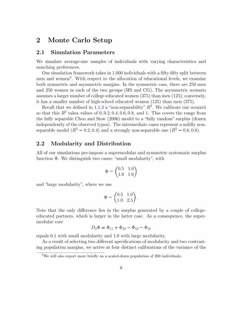
Recall that we defined in 1.1.3 a “non-separability”R2. We calibrate our scenariiso that this R2 takes values of 0, 0.2, 0.4, 0.6, 0.8, and 1. This covers the range fromthe fully separable Choo and Siow (2006) model to a “fully random” surplus (drawnindependently of the observed types). The intermediate cases represent a mildly non-separable model (R2 � 0.2, 0.4) and a strongly non-separable one (R2 � 0.6, 0.8).

2.2 Modularity and Distribution

All of our simulations pre-impose a supermodular and symmetric systematic surplusfunction Φ. We distinguish two cases: “small modularity”, with

Φ ��

0.5 1.01.0 1.6

and “large modularity”, where we use

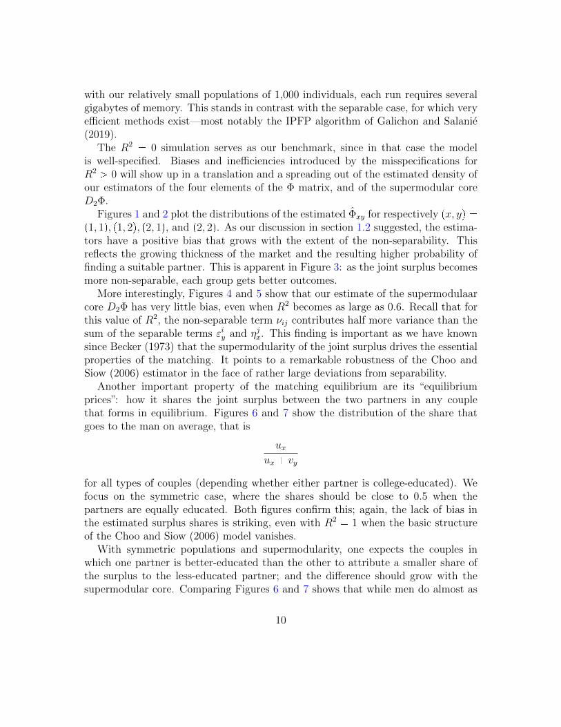
Φ ��

0.5 1.01.0 2.5

.

Note that the only difference lies in the surplus generated by a couple of college-educated partners, which is larger in the latter case. As a consequence, the super-modular core

D2Φ � Φ11 � Φ22 � Φ12 � Φ21

equals 0.1 with small modularity and 1.0 with large modularity.As a result of selecting two different specifications of modularity and two contrast-

ing population margins, we arrive at four distinct calibrations of the variance of the

3We will also report more briefly on a scaled-down population of 200 individuals.

8

systematic surplus Φ. In the “large market” limit of the separable Choo and Siow(2006) model when R2 � 0, the estimate of the variance of Φ in the case of smallmodularity is about 0.357 with symmetric margins and roughly 0.336 with asymmet-ric margins. In the case of large modularity, they are more than twice as high: about0.856 with symmetric margins and roughly 0.716 with asymmetric margins.

To complete the description of our simulation, we need to describe the specificationof the ε, η, and (for the non-fully separable cases R2 ¡ 0) also ν. We choose to drawall εiy, η

jx, and νij independently from the centered standard type I extreme value

distribution such that when R2 � 0, this is just the Choo and Siow (2006) model;scenarii with positive R2 explore its robustness to deviations from separability.

For each simulation scenario, we generate 1,000 datasets. Table 1 summarizes thesimulation scenarii.

Population: 1,000 (Separable) R2 � 0Draws: 1,000 (Non-Separable) R2 � 0.2, 0.4, 0.6, 0.8, 1Modularity: Small or Large

Symmetric Margins Asymmetric Margins

Share of Share ofCount Population Count Population

Men HS (x � 1) 250 25% 375 37.5%Men CG (x � 2) 250 25% 125 12.5%

Women HS (y � 1) 250 25% 125 12.5%Women CG (y � 2) 250 25% 375 37.5%

Table 1: Simulation Parameters

3 Monte Carlo Results

The combination of six values of R2, symmetric or asymmetric populations, andtwo modularity subcases generates 24 different scenarii. As going through all of ourresults would quickly bore the reader, we focus on the most striking ones. Sometimeswe only show plots for the small modularity/symmetric margins case to save space.

With non-separable surplus, the only way we know of solving for the equilibriummatching is to solve the linear programming problem associated with the primal(maximizing the total surplus) or dual (minimizing the sum of utilities under thestability constraints). We used the R interface of the free academic version of theGurobi software4 for this purpose. The algorithm converges very robustly. Even

4Gurobi (2019).

9

with our relatively small populations of 1,000 individuals, each run requires severalgigabytes of memory. This stands in contrast with the separable case, for which veryefficient methods exist—most notably the IPFP algorithm of Galichon and Salanie(2019).

The R2 � 0 simulation serves as our benchmark, since in that case the modelis well-specified. Biases and inefficiencies introduced by the misspecifications forR2 ¡ 0 will show up in a translation and a spreading out of the estimated density ofour estimators of the four elements of the Φ matrix, and of the supermodular coreD2Φ.

Figures 1 and 2 plot the distributions of the estimated Φxy for respectively px, yq �p1, 1q, p1, 2q, p2, 1q, and p2, 2q. As our discussion in section 1.2 suggested, the estima-tors have a positive bias that grows with the extent of the non-separability. Thisreflects the growing thickness of the market and the resulting higher probability offinding a suitable partner. This is apparent in Figure 3: as the joint surplus becomesmore non-separable, each group gets better outcomes.

More interestingly, Figures 4 and 5 show that our estimate of the supermodulaarcore D2Φ has very little bias, even when R2 becomes as large as 0.6. Recall that forthis value of R2, the non-separable term νij contributes half more variance than thesum of the separable terms εiy and ηjx. This finding is important as we have knownsince Becker (1973) that the supermodularity of the joint surplus drives the essentialproperties of the matching. It points to a remarkable robustness of the Choo andSiow (2006) estimator in the face of rather large deviations from separability.

Another important property of the matching equilibrium are its “equilibriumprices”: how it shares the joint surplus between the two partners in any couplethat forms in equilibrium. Figures 6 and 7 show the distribution of the share thatgoes to the man on average, that is

uxux � vy

for all types of couples (depending whether either partner is college-educated). Wefocus on the symmetric case, where the shares should be close to 0.5 when thepartners are equally educated. Both figures confirm this; again, the lack of bias inthe estimated surplus shares is striking, even with R2 � 1 when the basic structureof the Choo and Siow (2006) model vanishes.

With symmetric populations and supermodularity, one expects the couples inwhich one partner is better-educated than the other to attribute a smaller share ofthe surplus to the less-educated partner; and the difference should grow with thesupermodular core. Comparing Figures 6 and 7 shows that while men do almost as

10

well with M � 1, F � 2 as with M � 2, F � 1 when the modularity is small, thedifference becomes more noticeable with large modularity.

Since solving the linear programming problem is much more expensive than usingthe Iterative Proportional Fitting Procedure (IPFP) algorithm proposed by Galichonand Salanie (2019), it is also interesting to compare their performances in our simu-lation runs. While we already know that IPFP is much faster (and uses very littlememory), it is only rigorously valid in the “large market” limit when the number ofindividuals goes to infinity. Figure 8 shows that even with our population size of1,000, IPFP performs remarkably well: it yields equilibrium matching probabilitiesµxy that are very close to the mode of the distribution of the Gurobi results for thefinite-population case.

We also ran a set of simulations with only 200 individuals. The results are basicallysimilar as with 1,000 individuals, with more variation across runs as expected.

11

Figure 1: Estimates of Φ—small modularity

12

Figure 2: Estimates of Φ—large modularity

13

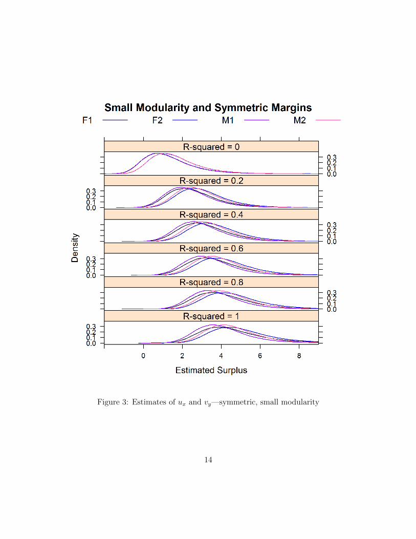
Figure 3: Estimates of ux and vy—symmetric, small modularity

14

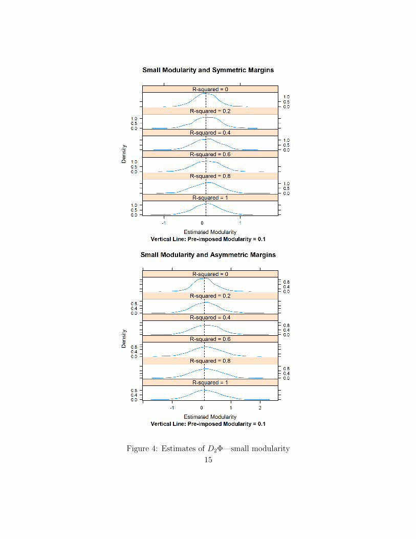
Figure 4: Estimates of D2Φ—small modularity

15

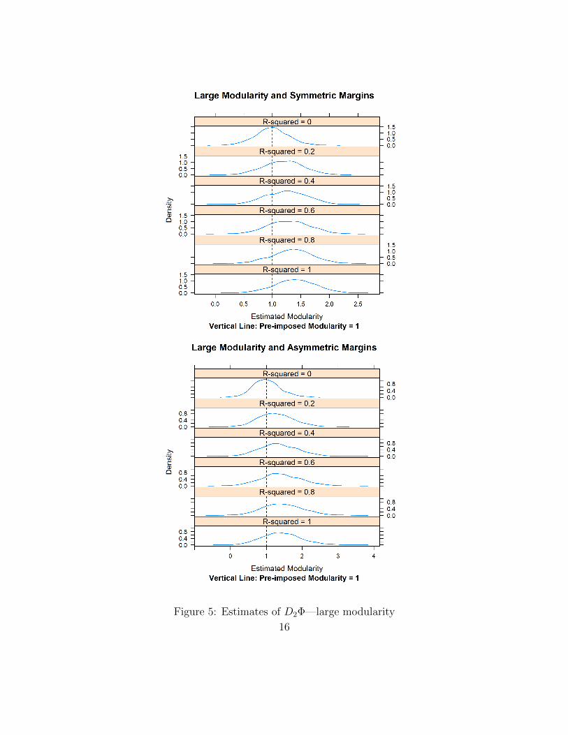
Figure 5: Estimates of D2Φ—large modularity

16

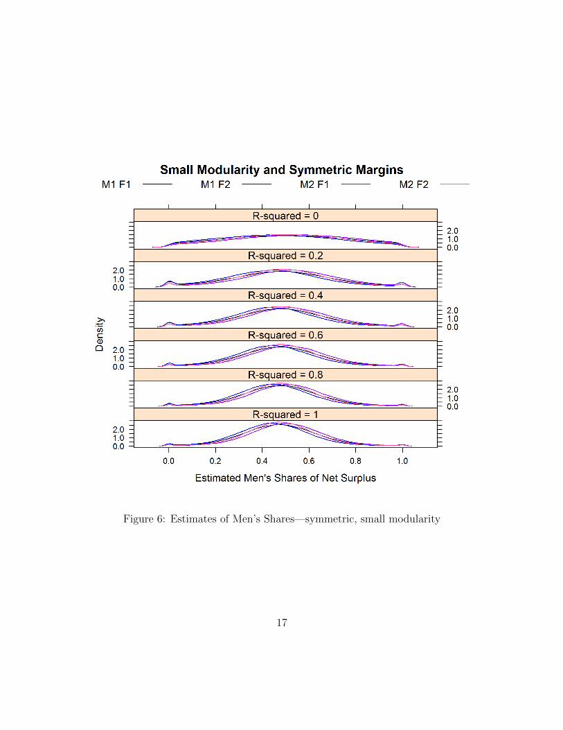
Figure 6: Estimates of Men’s Shares—symmetric, small modularity

17

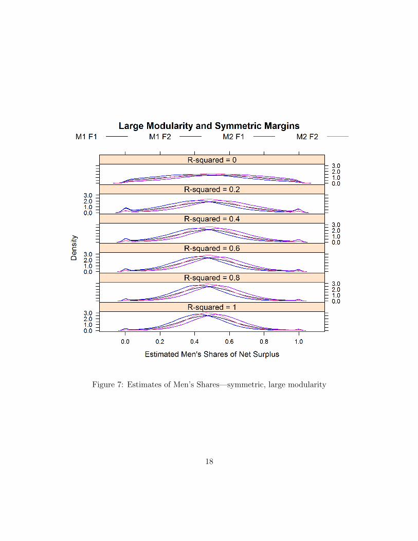
Figure 7: Estimates of Men’s Shares—symmetric, large modularity

18

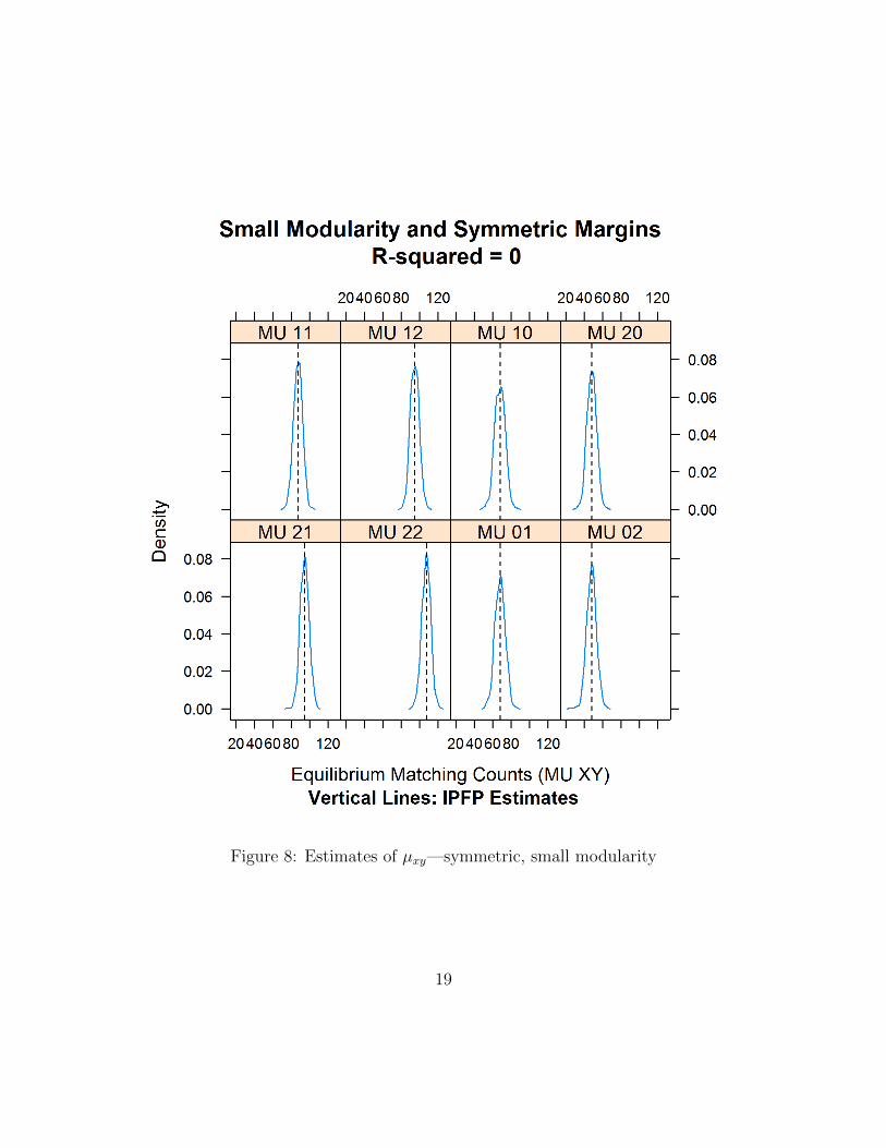
Figure 8: Estimates of µxy—symmetric, small modularity

19

Concluding Remarks

Even with our set of 24 scenarii, we have only explored a small area of the parameterspace. Our conclusions are encouraging for separable models, however: even thoughthey rule out interactions between unobservable characteristics, the induced misspec-ification biases do not seem to be severe. Estimating a separable, Choo and Siow(2006) model on data that may have been generated by a non-separable model doeslittle apparent harm to our ability to get reliable estimates of the most economicallyimportant statistics: the supermodular core and the surplus shares.

References

Becker, G. (1973): “A theory of marriage, part I,” Journal of Political Economy,81, 813–846.

Chiappori, P.-A., and B. Salanie (2016): “The Econometrics of Matching Mod-els,” Journal of Economic Literature, 54, 832–861.

Chiappori, P.-A., B. Salanie, and Y. Weiss (2017): “Partner Choice, Invest-ment in Children, and the Marital College Premium,”American Economic Review,107, 2109–67.

Choo, E., and A. Siow (2006): “Who Marries Whom and Why,” Journal of Po-litical Economy, 114, 175–201.

Ciscato, E., A. Galichon, and M. Gousse (2019): “Like Attract Like: A Struc-tural Comparison of Homogamy Across Same-Sex and Different-Sex Households,”Journal of Political Economy, Forthcoming.

Dupuy, A., and A. Galichon (2014): “Personality traits and the marriage mar-ket,” Journal of Political Economy, 122, 1271–1319.

Galichon, A., S. Kominers, and S. Weber (2019): “Costly Concessions: AnEmpirical Framework for Matching with Imperfectly Transferable Utility,”Journalof Political Economy, Forthcoming.

Galichon, A., and B. Salanie (2017): “The Econometrics and Some Properties ofSeparable Matching Models,”American Economic Review Papers and Proceedings,107, 251–255.

20

Galichon, A., and B. Salanie (2019): “Cupid’s Invisible Hand: Social Surplusand Identification in Matching Models,” Columbia University mimeo.

Gurobi (2019): “Gurobi Optimizer Reference Manual,” Discussion paper, GurobiOptimization, Inc.

Menzel, K. (2015): “Large Matching Markets as Two-Sided Demand Systems,”Econometrica, 83, 897–941.

Mourifie, I. (2019): “A Marriage Matching Function with Flexible Spillover andSubstitution Patterns,” Economic Theory, 67, 421–461.

Mourifie, I., and A. Siow (2017): “The Cobb Douglas Marriage Matching func-tion: Marriage Matching with Peer and Scale Effects,” University of Torontomimeo.

21