random ferns for keypoint recognition, image matching and...
TRANSCRIPT

CENTER FOR
MACHINE PERCEPTION
CZECH TECHNICAL
UNIVERSITY
RESEARCH
REPO
RT
ISSN
1213
-236
5
Random Ferns for KeypointRecognition, Image Matching andTracking – Implementation and
Experiments
Erik Derner, Tomas Svoboda,Karel Zimmermann
[email protected], [email protected],[email protected]
CTU–CMP–2010–16
November 3, 2010
Available atftp://cmp.felk.cvut.cz/pub/cmp/articles/svoboda/Derner-TR-2010-16.pdf
The authors were supported by EC project FP7-ICT-247870 NIFTiand by the Czech Science Foundation under project P103/10/1585.Any opinions expressed in this paper do not necessarily reflect theviews of the European Community. The Community is not liable
for any use that may be made of the information contained herein.
Research Reports of CMP, Czech Technical University in Prague, No. 16, 2010
Published by
Center for Machine Perception, Department of CyberneticsFaculty of Electrical Engineering, Czech Technical University
Technicka 2, 166 27 Prague 6, Czech Republicfax +420 2 2435 7385, phone +420 2 2435 7637, www: http://cmp.felk.cvut.cz

Random Ferns for Keypoint Recognition,Image Matching and Tracking –
Implementation and Experiments
Erik Derner, Tomas Svoboda, Karel Zimmermann
November 3, 2010
Abstract
We have implemented a ferns-based classifier in MATLAB and ap-plied it in image matching, object detection and tracking applications.We improve recognition performance, especially for scale changes. Ad-ditional modifications should help to overcome Harris corner detectorinaccuracy and improve RANSAC homography estimation. We per-formed experiments with various real-world images and we show thatour classifier is able to handle significant perspective changes.

Contents
1 Introduction 3
2 Ferns: Learning and Classification 32.1 Learning . . . . . . . . . . . . . . . . . . . . . . . . . . . . . . 32.2 Classification . . . . . . . . . . . . . . . . . . . . . . . . . . . 5
3 Implementation 63.1 Learning . . . . . . . . . . . . . . . . . . . . . . . . . . . . . . 7
3.1.1 Transformation parameters . . . . . . . . . . . . . . . . 83.1.2 Post-scaling . . . . . . . . . . . . . . . . . . . . . . . . 8
3.2 Classification . . . . . . . . . . . . . . . . . . . . . . . . . . . 83.2.1 Matching . . . . . . . . . . . . . . . . . . . . . . . . . 93.2.2 Finding object in a scene . . . . . . . . . . . . . . . . . 113.2.3 Tracking . . . . . . . . . . . . . . . . . . . . . . . . . . 11
4 Experiments 134.1 Tracking and object detection . . . . . . . . . . . . . . . . . . 13
4.1.1 Generated transformations . . . . . . . . . . . . . . . . 134.1.2 Ground truth sequences . . . . . . . . . . . . . . . . . 144.1.3 Ladybug sequences . . . . . . . . . . . . . . . . . . . . 17
4.2 Matching . . . . . . . . . . . . . . . . . . . . . . . . . . . . . 23
5 Conclusion 25
1 Introduction
Image recognition, matching and tracking belong to the most frequent com-puter vision tasks. We have implemented a complete classifier framework inMATLAB capable of these applications and thoroughly tested it. Sampleoutput of our classifier is on Figure 1.
At first, distinctive image locations – keypoints – are determined by theHarris corner detector [3]. Descriptors are based on comparison of imageintensities in randomly chosen pixel pairs around these keypoints. Findingtentative matches is based on Naive Bayesian classifier. In object detectionand tracking applications, RANSAC [2] is used for fitting of geometricalmodel.
The key component of the learning and classification process is the patchdescription. Patches around keypoints are evaluated by comparison of inten-sities in randomly formed pixel pairs called binary features. Many learningsamples are generated for each class (patch) during offline learning phase bytransforming the model image. The patches are evaluated in each transfor-mation and probabilities of certain values of the features are used as patchdescriptors. Joint probability of all binary features would require extremeamount of memory, as 2N values (N represents number of binary features)would have to be stored for each class. Assuming independence of all binaryfeatures would rapidly reduce necessary amount of memory, but it completelyignores the correlation between features. The compromise consists in parti-tioning binary features into M groups of size S = N
Mcalled ferns. Further
information can be found in [1] and in [4], section III.
2 Ferns: Learning and Classification
In this section, we will describe the algorithm we used for learning and clas-sification. Source code description will follow in section 3. The algorithmswere implemented in MATLAB version 7.8 and tested in MATLAB version7.8 and 7.9.
2.1 Learning
At first, the model image is converted to greyscale (if necessary) and sur-rounded with free space (black pixels) to prevent index overflow when eval-uating the patches in transformed image samples.
After that, Harris corner detector finds keypoints in the model image.Keypoints too close to the image borders (closer than half of the patch size
3

Figure 1: Finding correspondences (yellow lines), object detection (greenrectangle). Blue crosses in the query image represent Harris keypoints. Greenstars in the model image are correctly classified classes, while the red onesare incorrect.
in respective direction) are removed, the rest represent classes. Classes areidentified by index in a variable containing their coordinates.
The model image is transformed in many ways to simulate possible ap-pearance of the object in query images (scenes). Affine transformation ma-trices are generated for all combinations of given values of θ, φ and λ1,2 inthe formula
T = RθR−φdiag(λ1, λ2)Rφ , (1)
where R represents rotation by the subscripted angle, λ1,2 represent scaling.
For a given patch size, the coordinates of pixel pairs forming binary fea-tures are randomly chosen in range from −hx to hx horizontally and from−hy to hy vertically (where h represents half size of a patch in respectivedirection) and randomly partitioned to ferns.
Now, we describe the main loop over all generated transformations. Atfirst, the image and the keypoints’ coordinates are transformed by the giventransformation matrix. Gaussian noise with zero mean and large variance 25(for intensity values from 0 to 255) is added to image intensities to increaserobustness. Additionally, Gaussian smoothing with a mask of 7×7 is applied.
The core of the algorithm consists in classification of patches in the giventransformation. Binary features within a fern are evaluated, i.e., the intensi-ties of the two pixels within a binary feature are compared and evaluation isreturned – 1 if the intensity of the first pixel in the pair is smaller than the
4

intensity of the other one, 0 otherwise. Binary number formed by ‘concate-nating’ evaluations of features within a fern is converted to decimal represen-tation and 1 is added, so that the evaluation can be used as index. This isdone with all ferns on all patches (classes). The number of occurences of par-ticular fern evaluations is stored for each fern of each class and finally, afterrepeating the whole process for all transformations, recalculated to probabil-ity (all values are divided by a constant: number of samples + 2fern size). Theevaluations that have never occured are treated as if they have occured onceto prevent classification failure when calculating product of probabilities.
If requested, all classes’ coordinates are translated by a given value in alleight directions (horizontally, vertically and diagonally), thus the core of thelearning algorithm is run eight more times. This improvement should helpovercome possible Harris detector inaccuracy.
To improve classification, we added post-scaling, which extends and refinesthe scaling range given by λ1,2 values in (1). To make the classification faster,the post-scale probabilities are calculated already in the learning phase. Thescale change is simulated by resizing ferns. It can be also described as learningferns on different patch sizes. Resizing is done by the same coefficient in bothdirections (i.e., aspect ratio is retained).
2.2 Classification
After learning the ferns probability model, classification can be run in one ofthe three modes: matching, finding object in a scene and tracking.
Matching mode is used to find correspondences between keypoints inthe model (classes) and in the query image (yellow lines on Figure 1). Bydefault, the most similar class is found for each patch around keypoints in thequery image. Our classifier also allows matching in opposite direction, wherethe most similar keypoint in the query image is found for each class. Asthere are usually less classes than keypoints in the query image, the oppositeapproach is generally faster, but the recognition rate decreases.
Finding mode is intended for object detection applications. RANSACis used to estimate homography (transformation matrix) from found corre-spondences between model classes and keypoints in the query image. Asa by-product, correctly matched correspondences are determined as inliers,incorrect as outliers. The computed homography essentially finds exact lo-cation of the sought object, see the green rectangle in Figure 1.
Tracking mode is suitable for object tracking in image sequences, wherethe difference of successive images is rather small. This mode extends thefinding mode by restriction of keypoints translation between two succeedingimages (maximal translation may be set by user). Additionally, the object
5
is first searched in surrounding of its position in the previous image in thesequence. If the object is not found in the restricted area, the whole imageis searched through (as in the finding mode).
Now, we describe the classification process. Firstly, the image to be clas-sified is converted to greyscale (if necessary) and keypoints – Harris cornersare detected (in bounded area in the tracking mode according to previousobject location, else in the whole image). Keypoints too close to the im-age borders (closer than half of the patch size in respective direction) areremoved.
Correspondences between classes in the model image and keypoints in thequery image are determined this way: Patches around all keypoints are eval-uated using the same ferns that were used for learning. The prior (learned)probabilities of the acquired evaluations of all ferns are loaded for each classand multiplied, the particular keypoint (patch) is then assigned to the classwith the largest product. This can be formulated as finding
ci = argmaxci
M∏k=1
P (fk | C = ci) , (2)
where fk represents evaluation of kth fern, ci represents ith class and M isnumber of ferns. Maximum translation of each keypoint between the cur-rent and previously classified image is limited in the tracking mode, whichrestrains classes the keypoint can be assigned to.
In the finding and tracking mode, if not enough inliers were found to besure that RANSAC returned correct homography (e.g. less than 10 inliers),the whole process is repeated for succeeding post-scales. In case that allpost-scales were tried and the given number of inliers was achieved for noneof them, the post-scale with the highest number of inliers is taken as thebest. Classification of the next image in the tracking mode will begin withthe best post-scale used for the last image.
If the refine mode is on, the classification may be re-run with higherRANSAC iteration limit to achieve better results when not sure about thecorrectness of the previously calculated homography. More about the refinemode can be found in section 3.2.
3 Implementation
As the process of image recognition consists of two main phases, learningand classification, there are two main functions, f learn for learning andf find for classification. Demonstration scripts are also distributed, detaileddescription can be found in the succeeding sections.
6

Brief overview The script demo ferns.m provides a brief overview of ob-ject detection using our classifier. The image specified in input image isdisplayed, user selects the object to be learned by dragging a rectangle withmouse. After the learning and classification process finishes, the result isdisplayed. The estimated object position is marked green. Blue crosses inthe query image indicate found keypoints (Harris corners). Red stars in themodel image represent classes that were determined by RANSAC as outliers,while green stars are inliers. Matching of correctly classified pairs (inliers) isdrawn as yellow lines (Figure 1).
Sample data We recommend downloading ground truth image sequences1
to take full advantage of the demonstration scripts. Each of the * img and* gt archives should be extracted to separate directory. Directory structurefor downloaded archives extraction is already prepared in this package inthe directory testdata. Images used for learning named img learn.jpg arestored in * img directories in testdata in this package.
3.1 Learning
Function f learn is used to learn ferns model on an input image. The syntaxismodel = f learn(im, par),where im is a model image (to be learned) represented as uint8 matrix. Colorimage will be automatically converted to greyscale. It is possible to set thepathname of the image instead, then the image is automatically read in therequired format. Structure par contains parameters for learning. Descriptionof the parameters can be found in the beginning of f learn.m. All parametersare compulsory.
The fields of the output structure model are also described in the begin-ning of f learn.m, but none of the fields has to be handled by user.
Sample configuration of learning is in demo learn.m. The script consistsof setting all parameters and calling the function f learn in the end. Thelearned model is stored in the variable model. It can be saved by the MAT-LAB commandsave filename model
and later reloaded and repeatedly used for classification by callingload filename.This is beneficial to save time.
1http://cmp.felk.cvut.cz/demos/Tracking/linTrack/data/index.html
7

3.1.1 Transformation parameters
The image is transformed in the learning phase in various ways to ensurerobustness. Transformation parameters used in (1) are set in the struc-ture par.tform. All combinations of values in the fields of par.tform
(theta values, phi values, lambda1 values, lambda2 values) are gener-ated. It means that the time necessary for learning rapidly increases whensetting more values. Total number of learning samples can be calculated asthe product of sizes of all par.tform fields.
If you would like to use random values in par.tform fields instead ofsetting them explicitly, you can generate them by the supplied functiongen rand. This function takes three parameters:rand array = gen rand(min value, max value, count),where the number range is specified by min value and max value. The func-tion generates 1-by-count array of random numbers in the given range.
3.1.2 Post-scaling
Post-scales used for better coping with the searched object’s scale changes(see 2.1) are set in the field par.post resize as a row vector. For instance,the value 0.5 represents resizing the image to half size. It is important toleave 1 as the first value in the vector. Sample setting can be found indemo learn.m.
Post-scaling can be turned off by settingpar.post resize = 1.
3.2 Classification
After learning ferns (or loading a previously learned model), it is possibleto begin the classification. Function f find, which is the main function forclassification, supports three modes: matching, finding object in a scene andtracking.
The syntax of the function is[corners f data] = f find(im, model, par, par cl),where im is the image to be classified. As in f learn, it can be eitheruint8 matrix or a pathname of the image, color image will be automaticallyconverted to greyscale. Variable model is the learned ferns model (outputfrom f learn), par are parameters used for learning. If par is no more inthe variable environment (e.g. when loading saved model), it can be fullyrestored from model.par.
Parameters for classification are set in the structure par cl. Unlike in the
8

learning phase, all the parameters are optional. Anyway, we strongly recom-mend setting the essential values manually. Detailed parameters descriptionand default values, which are used if the parameters are not explicitly set,can be found in the beginning of f find.m.
Function f find has two output arguments: corners and f data. Thevariable corners is a 4×2 matrix, in each row there are x- and y-coordinatesof the corner of the estimated area, where the object should be located. Ifthe object is not found (or in the matching mode), corners is filled by zeros.
Matched pairs are stored in the variable f data.matching data in form of6-by-N matrix, where first two rows contain class coordinates (in the model),4th and 5th row contain keypoint coordinates (in the query image). If not inthe matching mode, it is possible to extract the pairs that were classified byRANSAC as inliers. These ‘correct’ pairs (correspondences) are stored in thevariable f data.corresp, which is of the same structure as matching data.
Other fields of f data are described in the beginning of f find.m.
Refine mode In the refine mode, if less than par cl.ransac inls good
inliers are found, f find is recalled with higher RANSAC iteration limitset in par cl.ransac max iter fine. If par cl.ransac inls refine all
or less inliers were found in the first run, f find tries all post-scales in thesecond run, otherwise it takes only the best post-scale from the first run (theone with the most inliers). The refine mode is turned on by explicitly settingthe par cl.ransac max iter fine value. This mode increases recognitionperformance, but decreases speed. It is available in the finding and trackingmode.
3.2.1 Matching
One of the possible usages of f find is matching, i.e., finding correspondencesbetween keypoints in the model (classes) and in the query image.
Sample matching task is in demo match. The image for classification isselected by setting path (PATH IMG) and index (IMG INDEX). The functionf find is run in matching mode by settingpar cl.matching mode = true.
The script demo match shows a figure with found correspondences (Figure2). Matched pairs can be displayed by callingdisp(f data.matching data).
9
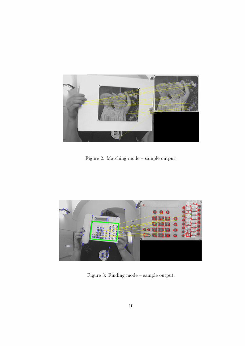
Figure 2: Matching mode – sample output.
Figure 3: Finding mode – sample output.
10

3.2.2 Finding object in a scene
Using f find to find an object in a scene is demonstrated in demo find. Thisscript also uses some features of tracking. Unlike the other two modes, nospecification of finding mode usage in par cl is necessary as this mode istaken as default.
The script runs a test sequence on images in directory PATH IMG start-ing with MIN INDEX and continuously increasing the index by STEP untilMAX INDEX is reached. The images are classified and corners from f find
are compared with ground truth stored in PATH GT directory. The variableCORR DIST LIMIT is used to set the maximum position difference (both hori-zontally and vertically) of all corners in comparison to the ground truth. Thearea defined by corners is drawn green if it matches ground truth, otherwisethe color is red. Blue crosses in the query image indicate found keypoints(Harris corners). Red stars in the model represent classes that were deter-mined by RANSAC as outliers, while green stars are inliers. Matching ofcorrectly classified pairs (inliers) is drawn as yellow lines (Figure 3).
Classification statistics are saved during the test sequence to the variableresults. As the script finishes, brief summary is displayed and a figureshows, how many times was each class classified as inlier. Detailed resultscan be displayed by typingparse results(results).Used post-scale indicates the index of the scale in par.post resize that wasfinally used. If RANSAC returned enough inliers (par cl.ransac inls good
or more), the index is stored as it is. The value is increased by 100 to indicatethat RANSAC found less than par cl.ransac inls good inliers, i.e., f find
tried all post-scales and enough inliers were found in none of them.
It is possible to save displayed figures as EPS images and results as a textfile for later inspection by settingSAVE OUTPUT = true.All files are saved to the directory specified in PATH OUT. Please note thatthe output directory has to be manually created.
3.2.3 Tracking
Tracking mode is similar to the finding mode. The demonstration scriptdemo track uses cell mode, which enables the user to easily re-run only theclassification by evaluating the last cell ‘Classification’ with different param-eters without repetitive learning. This script goes through the whole processof learning and recognition, i.e., no previous learning using demo learn isnecessary (unlike the preceding scripts).
11
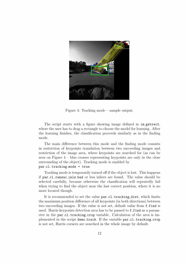
Figure 4: Tracking mode – sample output.
The script starts with a figure showing image defined in im getrect,where the user has to drag a rectangle to choose the model for learning. Afterthe learning finishes, the classification proceeds similarly as in the findingmode.
The main difference between this mode and the finding mode consistsin restriction of keypoints translation between two succeeding images andrestriction of the image area, where keypoints are searched for (as can beseen on Figure 4 – blue crosses representing keypoints are only in the closesurrounding of the object). Tracking mode is enabled bypar cl.tracking mode = true.
Tracking mode is temporarily turned off if the object is lost. This happensif par cl.ransac inls bad or less inliers are found. The value should beselected carefully, because otherwise the classification will repeatedly failwhen trying to find the object near the last correct position, where it is nomore located though.
It is recommended to set the value par cl.tracking dist, which limitsthe maximum position difference of all keypoints (in both directions) betweentwo succeeding images. If the value is not set, default value from f find isused. Harris keypoints detection area has to be passed to f find as a param-eter in the par cl.tracking crop variable. Calculation of the area is im-plemented in the script demo track. If the variable par cl.tracking crop
is not set, Harris corners are searched in the whole image by default.
12

a b c
Figure 5: Generated transformations experiment – images: a – animals, b –costume, c – museum. Yellow rectangle specifies the object that is localizedin transformed images.
4 Experiments
We performed experiments on various image sets to evaluate our classifierand the modifications not described in [4] that we introduced – post-scaling,refine mode, selecting pairs with the highest probability values for RANSAC,finding correspondences for model classes instead of query image keypointsand keypoints translation in the learning stage.
4.1 Tracking and object detection
4.1.1 Generated transformations
In this experiment, we wanted to evaluate our classifier on basic transforma-tions as scale and rotation. Aditionally, we tested how selecting a number ofpairs with the highest probability product for evaluation by RANSAC affectsthe recognition rate. At first, we selected objects in the images on Figure5 (marked yellow). Then we generated several transformations and let ourclassifier determine the objects’ positions in the transformed images.
The transformation matrix is calcuated using (1). This allows us to easilyobserve the influence of rotation and scaling on the recognition rate. Addi-tionally, we can precisely determine the correct object position in the trans-formed image, because we know the transformed object coordinates.
Learning on 900 samples took about 5 minutes, training transformationsconsisted of rotation from 0 to 360◦ with step 10◦ and scaling from 0.5 to1.5 with step 0.25 in both directions. Shear was not used in this experiment(φ = 0 in (1)). 32×32 px patches were evaluated by 30 ferns of size 11. Usingnon-MEX Harris corner detector with threshold 10000, 51 classes were foundon image animals, 62 classes on image costume and 39 classes on image
13
museum. Post-scaling coefficients variable (par.post resize) was set to[1 0.5 0.75 1.25 1.5 1.75 2], translation of Harris corners was disabled(par.surrounding = 0).
Classification ran in finding mode with default parameters except forRANSAC maximum iterations thresholds that were set to ransac max iter
= 1000 and ransac max iter fine = 20000 (which implies that the refinemode was on). Query image was evaluated as correct if all four corners werefound correctly with tolerance of 20 pixels (both horizontally and vertically).
Table 1 shows results of classification for rotation with no scaling (100 %),resizing to 75 % and 150 %. It is obvious that rotation has no negativeeffect on the object finding success. Some detection failures for the imagemuseum in rotations combined with scaling could be caused by lower numberof classes and by repetitive objects – windows, which make the classificationmore difficult.
Simple scaling (without rotation) yielded rather worse results (Table 2).The object was correctly found on none of the 3× enlarged images, simi-larly for the reduced images animals and museum. This is mainly causedby the Harris corner detector behavior, as the number and position of foundHarris corners considerably differs for various scales. Better results may beachieved by changing the Harris detector threshold for extensive scale differ-ences. Stable keypoints selection in the learning phase would help overcomethis problem, which is one of the most important improvements to be imple-mented in the future.
We also tried choosing only the best correspondences for RANSAC. Thenumber of pairs with the highest probability product to be evaluated byRANSAC is determined in the field n best matches for ransac of the pa-rameters structure par cl. The image museum was used for this experiment.Recognition performance rapidly decreased for very low values (about 1.5×number of classes and less), but for values about 2.5× number of classes,we achieved better results than without this feature. There is no generalrecommendation whether to use this feature and what value should be set,but recognition performance improvement may be achieved with carefullyselected n best matches for ransac value.
4.1.2 Ground truth sequences
Three ground truth image sequences (Figure 6) available on2 – mouse pad(6946 VGA images), phone (2300 VGA images) and towel (3231 VGA images)– were used for object finding and tracking experiments. The objects are ma-
2http://cmp.felk.cvut.cz/demos/Tracking/linTrack/data/index.html
14
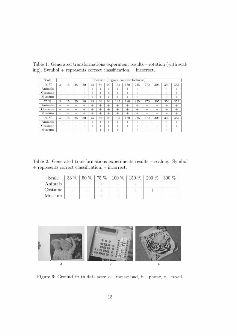
Table 1: Generated transformations experiment results – rotation (with scal-ing). Symbol + represents correct classification, – incorrect.
Scale Rotation (degrees counterclockwise)
100 % 5 15 25 30 45 60 90 135 180 225 270 305 350 355Animals + + + + + + + + + + + + + +Costume + + + + + + + + + + + + + +Museum + + + + + + + + + + + + + +
75 % 5 15 25 30 45 60 90 135 180 225 270 305 350 355Animals + + + + + + + + + + + + + +Costume + + + + + + + + + + + + + +Museum – + + + + + + + + + + + + +
150 % 5 15 25 30 45 60 90 135 180 225 270 305 350 355Animals + + + + + + + + + + + + + +Costume + + + + + + + + + + + + + +Museum – – + – – + + + – + + + + –
Table 2: Generated transformations experiments results – scaling. Symbol+ represents correct classification, – incorrect.
Scale 33 % 50 % 75 % 100 % 150 % 200 % 300 %Animals – – + + + – –Costume + + + + + + –Museum – – + + – – –
a b c
Figure 6: Ground truth data sets: a – mouse pad, b – phone, c – towel.
15

nipulated in many ways in the sequences – rotated, taken further and closer,tilted, partially covered etc. We wanted to evaluate the impact of trackingmode, refine mode, post-scaling and their combinations on the recognitionperformance. With the provided ground truth data (corner coordinates of thesearched objects), it is easy to automatically determine whether the objectwas found correctly or not.
The classifier was learned on the img learn.jpg image for each sequence,which can be found in respective * img directories under testdata dis-tributed within this package. We used 30 ferns of size 11, Gaussian filterstandard deviation was 2, patches were 32 × 32 pixels in size and we usednon-MEX Harris corner detector with threshold 5000, which resulted in 60classes on mouse pad, 183 classes on phone and 112 classes on towel data set.13068 training samples were generated by rotation all around with step 10◦,shear (φ in (1)) 0 and two random values from 0 to 180◦ and scaling from0.5 to 1.5 with step 0.1 both horizontally and vertically. The translation ofHarris corners (par.surrounding) was set to 0 (no translation) and the post-scaling coefficients (par.post resize) were [1 0.5 0.75 1.25 1.5 1.75
2]. Learning with these parameters takes about 90 minutes on a standarddesktop computer.
All sequences were classified in five scenarios to compare results dependenton the usage of tracking/finding mode (t+/t−), refine mode on/off (r+/r−)and post-scaling on/off (p+/p−). Scenarios’ parameters are summarized inTable 3. Supplied scripts demo find (scenarios t−r+p+, t−r−p+ and t−r−p−)and demo track (scenarios t+r+p+ and t+r−p+) were used for classification.Each 5th image in the sequences was classified, which reduced the compu-tation time to one fifth while the results were still enough reliable. Weused default par cl values except for RANSAC maximum iterations thresh-olds, which were set to ransac max iter = 1000 and, in scenarios t−r+p+
and t+r+p+, ransac max iter fine = 20000. The tracking was run withtracking dist = 80. The script demo track was modified to better meetthe requirements of this experiment, i.e., the learning stage was removed andthe initial corners’ coordinates were set manually (instead of retrieving themautomatically using getrect when selecting the object to learn). The valueof par cl.ransac inls bad was manually increased by one from the defaultvalue in the tracking mode (i.e., in scenarios t+r+p+ and t+r−p+), becausewe found out that ‘resetting’ the tracking mode (temporarily turning it off,when the object position is lost) even when 5 inliers are found produces muchbetter results. Using the default value, it keeps ‘wrong’ tracking much longer,because with only 4 inliers, RANSAC often returns senseless homography.
Recognition performance of our classifier for each data set, i.e., in howmany images was the object correctly found, is summarized in Table 4. An
16
image is determined as correctly classified if all estimated corners’ coordinatesmatch the ground truth corners’ coordinates with maximum difference of 50pixels both vertically and horizontally. Such a high position tolerance isnecessary because of the fact that the learned model image (img learn.jpg)corners are being localized in the query images (as it would be useful inreal applications), but the ground truth data contain crosses’ coordinatesin the mouse pad and phone sequences. This issue doesn’t affect the towelsequence, but we want to keep the value the same for all experiments forbetter comparison.
Post-scaling is enabled in scenario t−r−p+ and disabled in scenario t−r−p−,while all other parameters are the same. Here we show that the post-scalingwe used in our implementation improved the results by 52 % for mouse pad,by 359 % for phone and by 112 % for towel data set. Time consumption ofre-running RANSAC with very limited number of iterations (1000, becausethe refine mode is off in scenarios t−r−p+ and t−r−p−) is quite low.
The refine mode provides even much better results, which is obvious fromcomparison of the values in columns t−r+p+ and t−r−p+ (finding mode), orin columns t+r+p+ and t+r−p+ (tracking mode). Whether to enable the re-fine mode or not depends on the speed requirements of a certain application.Using non-MEX Harris corner detector, one image is generally classified inhundreds of milliseconds if the refine mode is disabled, but it may take sec-onds if the refine mode is on and refine is requested. For instance, on thedata set mouse pad, it takes about 200–400 ms if the first used scale returnedenough inliers or about 800 ms if all post-scales were tried, but it takes about5–6 seconds if refine is requested in the refine mode. (Only the computationtime is measured, not the disk and graphics operations.)
The tracking mode is useful in combination with disabled refine mode(scenario t+r−p+). It saves time (because Harris corners are generally searchedfor on a smaller area; even less than 100 ms may be necessary for an image)and produces slightly better results than the finding mode (scenario t−r−p+).If the refine mode is on, even a bit worse results are returned, when the track-ing mode is on (scenario t+r+p+). This could be caused by tracking failure,which spoils some images that are classified correctly in the finding mode(scenario t−r+p+), as RANSAC has enough iterations to estimate the cor-rect homography even without the support of tracking mode restrictions.
4.1.3 Ladybug sequences
Coping with high resolution real world images, background changes, low lightconditions and partial visibility of various objects were to be evaluated in
17

Table 3: Ground truth data sets experiments – parameters (+ on, – off).
t−r+p+ t−r−p+ t−r−p− t+r+p+ t+r−p+
Tracking mode – – – + +Refine mode + – – + –Post-scaling + + – + +
Table 4: Ground truth data sets experiments – recognition performance (%).
t−r+p+ t−r−p+ t−r−p− t+r+p+ t+r−p+
Mouse pad 92.16 76.33 50.14 90.50 79.86Phone 48.70 31.96 8.91 47.17 35.65Towel 93.82 88.56 78.98 92.43 91.19
another set of experiments done with ladybug image sequences. As Ladybug33
is a spherical multiple view motion camera, some experiments were done onsequences from a single camera, the others were run on panoramatic images.
Two data sets were used: vrakoviste taken on a scrapyard and dvoranafrom the school yard. Single camera shots were 1232 × 1616 pixels in size,panoramatic images were 5400 × 2700 pixels large. We used slightly mod-ified demo track with 30 ferns of size 11, patches were 40 × 40 pixels insize. Harris threshold was set to 10000 in most cases (non-MEX Harriscorner detector was used), but it was decreased in few cases to get moreclasses on dark objects. Learning on 441 samples with rotation 0 and 15◦
both clockwise and counterclockwise, shear (φ in (1)) 0, 15◦ and 165◦ andscaling from 0.7 to 1.3 with step 0.1 both horizontally and vertically tookabout 2–3 minutes. The rotation range was extended by additional valuesfor sequences with larger rotation changes. Translation of Harris corners(par.surrounding) was set to 0 (no translation) and the post-scaling coef-ficients (par.post resize) were [1 0.5 0.75 1.25 1.5 1.75 2]. Defaultpar cl values were used except for RANSAC maximum iterations thresholds,which were set to ransac max iter = 1000 and ransac max iter fine =
20000, ransac inls bad was set to 5. The variable tracking dist was setto 100.
Figure 7 shows results of experiments on images from a single camera onthe vrakoviste data set. Experiments a and b show a car with high contrasts
3http://www.ptgrey.com/products/ladybug3/index.asp
18
a
b
c
d
e
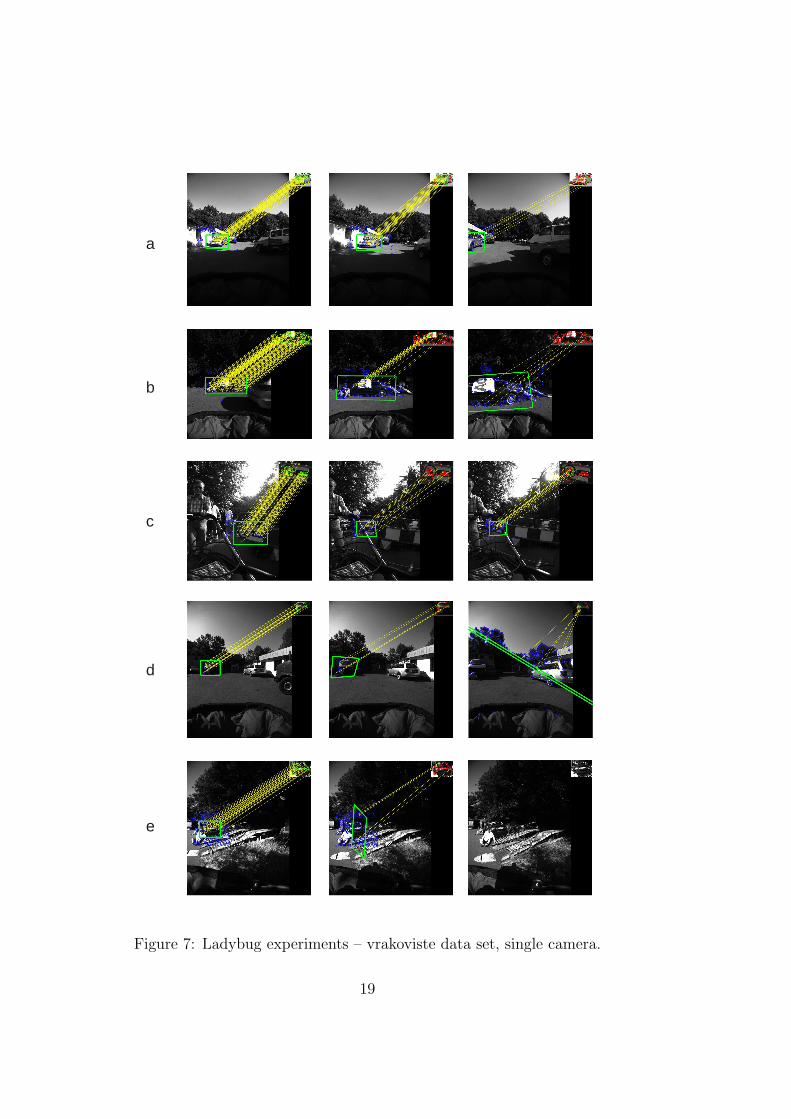
Figure 7: Ladybug experiments – vrakoviste data set, single camera.
19
and many classes, which gave very good results. Even when half of the caris out of the scene, it can still be recognized. In image set c, we show thatferns are very efficient for sign recognition, as the text and pictograms onthe sign provide many unambiguous classes. The sign is recognized well evenwhen partially covered. On the other hand, dark objects with too few Harriscorners (d), particularly in combination with considerably changing learnedsurrounding (e), returned worse results, we were able to track them only fora few frames of the sequences.
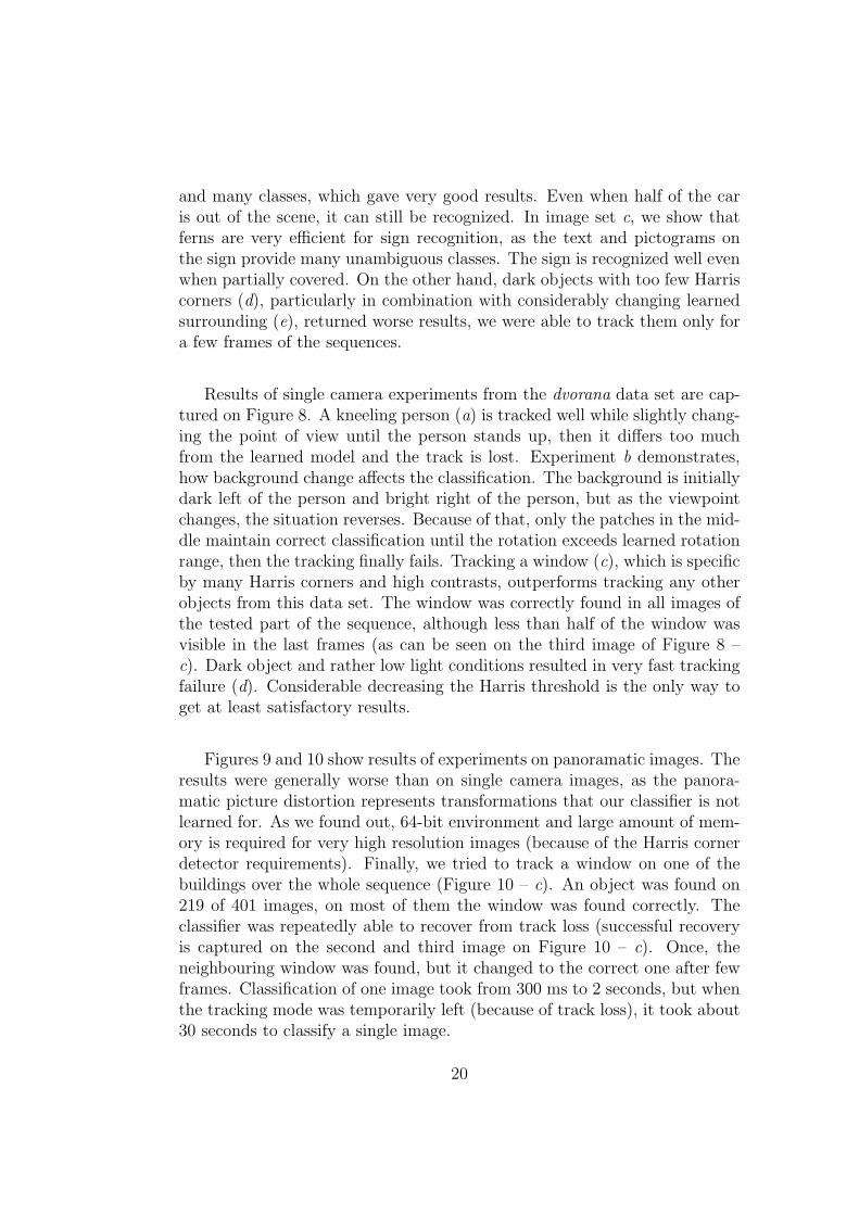
Results of single camera experiments from the dvorana data set are cap-tured on Figure 8. A kneeling person (a) is tracked well while slightly chang-ing the point of view until the person stands up, then it differs too muchfrom the learned model and the track is lost. Experiment b demonstrates,how background change affects the classification. The background is initiallydark left of the person and bright right of the person, but as the viewpointchanges, the situation reverses. Because of that, only the patches in the mid-dle maintain correct classification until the rotation exceeds learned rotationrange, then the tracking finally fails. Tracking a window (c), which is specificby many Harris corners and high contrasts, outperforms tracking any otherobjects from this data set. The window was correctly found in all images ofthe tested part of the sequence, although less than half of the window wasvisible in the last frames (as can be seen on the third image of Figure 8 –c). Dark object and rather low light conditions resulted in very fast trackingfailure (d). Considerable decreasing the Harris threshold is the only way toget at least satisfactory results.
Figures 9 and 10 show results of experiments on panoramatic images. Theresults were generally worse than on single camera images, as the panora-matic picture distortion represents transformations that our classifier is notlearned for. As we found out, 64-bit environment and large amount of mem-ory is required for very high resolution images (because of the Harris cornerdetector requirements). Finally, we tried to track a window on one of thebuildings over the whole sequence (Figure 10 – c). An object was found on219 of 401 images, on most of them the window was found correctly. Theclassifier was repeatedly able to recover from track loss (successful recoveryis captured on the second and third image on Figure 10 – c). Once, theneighbouring window was found, but it changed to the correct one after fewframes. Classification of one image took from 300 ms to 2 seconds, but whenthe tracking mode was temporarily left (because of track loss), it took about30 seconds to classify a single image.
20
a
b
c
d
Figure 8: Ladybug experiments – dvorana data set, single camera.
21

a
b
c
Figure 9: Ladybug experiments – vrakoviste data set, panoramatic view.
a
b
c
Figure 10: Ladybug experiments – dvorana data set, panoramatic view.
22
4.2 Matching
Using the generated images from section 4.1.1, we performed a few exper-iments also in the matching mode. Parameters for learning remained thesame. Recognition rate, i.e., how many classes from the learned model werecorrectly found in the query image, was measured for certain transformations.
We also tested our modifications – finding correspondences for modelclasses instead of query image keypoints and translation of keypoints in thelearning stage – which were not described in [4].
The classification in matching mode was performed with default f find
parameters. A class was evaluated as correctly classified if any keypointin the query image was correctly matched with the given class (admittinginaccuracy of 5 pixels both horizontally and vertically). There are generallymore keypoints in the query image than in the learned object (which isusually smaller than the query image). The most probable class is assignedto each keypoint, hence one class may be paired with more keypoints. Ifpar cl.corr from model is set to true, the best keypoint in the query imageis found for each class, therefore at most one keypoint can be paired with oneclass. This yields worse results than default finding the best class for eachkeypoint in the query image, unless the query image contains less keypointsthan number of classes. Our experiment confirms this, we got better resultsusing the default approach for all transformations except for resizing to 33%.
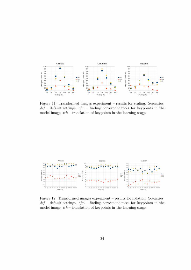
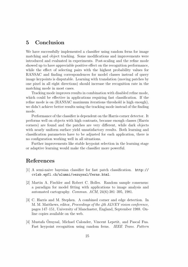
Comparison of recognition rate for different scales is on Figure 11, theeffect of rotation is shown on Figure 12. We used three scenarios to determinethe effect of our modifications. The experiments in scenario def were run withpar cl.corr from model = false and par.surrounding = 0. We changedpar cl.corr from model to true in scenario cfm to find out, how directionof correspondence finding affects the classification. Scenario trk differs fromdefault settings in scenario def by setting par.surrounding = 1, as we testedthe effect of learning with translation of keypoints in the model.
The results of classification when finding the best keypoint for each class(scenario cfm) were much worse than with the default settings (scenariodef) except for resizing to 33 % because of the previously mentioned rea-sons. Learning with translation of keypoints (scenario trk), which makes thelearning stage approx. 5× longer, brought slightly better results on average.However, there is no general recommendation whether to use learning withtranslation or not, as the classifier was in some cases less successful than inscenario def.
23
33 50 75 100 150 200 300
0
10
20
30
40
50
60
70
80
90
100
Animals
ABC
Scaling (%)
Re
cog
niti
on
ra
te (
%)
33 50 75 100 150 200 300
0
10
20
30
40
50
60
70
80
90
100
Costume
ABC
Scaling (%)
Re
cog
niti
on
ra
te (
%)
33 50 75 100 150 200 300
0
10
20
30
40
50
60
70
80
90
100
Museum
ABC
Scaling (%)
Re
cog
niti
on
ra
te (
%)
defcfmtrk
defcfmtrk
defcfmtrk
Figure 11: Transformed images experiment – results for scaling. Scenarios:def – default settings, cfm – finding correspondences for keypoints in themodel image, trk – translation of keypoints in the learning stage.
5 15 25 30 45 60 90 135 180 225 270 305 350 355
0
10
20
30
40
50
60
70
80
90
100
Animals
ABC
Rotation (°)
Re
cog
niti
on
ra
te (
%)
5 15 25 30 45 60 90 135 180 225 270 305 350 355
0
10
20
30
40
50
60
70
80
90
100
Costume
ABC
Rotation (°)
Re
cog
niti
on
ra
te (
%)
5 15 25 30 45 60 90 135 180 225 270 305 350 355
0
10
20
30
40
50
60
70
80
90
100
Museum
ABC
Rotation (°)
Re
cog
niti
on
ra
te (
%)
defcfmtrk
defcfmtrk
defcfmtrk
Figure 12: Transformed images experiment – results for rotation. Scenarios:def – default settings, cfm – finding correspondences for keypoints in themodel image, trk – translation of keypoints in the learning stage.
24
5 Conclusion
We have successfully implemented a classifier using random ferns for imagematching and object tracking. Some modifications and improvements wereintroduced and evaluated in experiments. Post-scaling and the refine modeshowed up to have appreciable positive effect on the recognition performance,while the effect of selecting pairs with the highest probability values forRANSAC and finding correspondences for model classes instead of queryimage keypoints is disputable. Learning with translation (moving patches byone pixel in all eight directions) should increase the recognition rate in thematching mode in most cases.
Tracking mode improves results in combination with disabled refine mode,which could be effective in applications requiring fast classification. If therefine mode is on (RANSAC maximum iterations threshold is high enough),we didn’t achieve better results using the tracking mode instead of the findingmode.
Performance of the classifier is dependent on the Harris corner detector. Itperforms well on objects with high contrasts, because enough classes (Harriscorners) are found and the patches are very different, while dark objectswith nearly uniform surface yield unsatisfactory results. Both learning andclassification parameters have to be adjusted for each application, there isno configuration working well in all situations.
Further improvements like stable keypoint selection in the learning stageor adaptive learning would make the classifier more powerful.
References
[1] A semi-naive bayesian classifier for fast patch classification. http://
cvlab.epfl.ch/alumni/oezuysal/ferns.html.
[2] Martin A. Fischler and Robert C. Bolles. Random sample consensus:a paradigm for model fitting with applications to image analysis andautomated cartography. Commun. ACM, 24(6):381–395, 1981.
[3] C. Harris and M. Stephen. A combined corner and edge detection. InM. M. Matthews, editor, Proceedings of the 4th ALVEY vision conference,pages 147–151, University of Manchaster, England, September 1988. On-line copies available on the web.
[4] Mustafa Ozuysal, Michael Calonder, Vincent Lepetit, and Pascal Fua.Fast keypoint recognition using random ferns. IEEE Trans. Pattern
25

Anal. Mach. Intell., 32(3):448–461, 2010. http://cvlab.epfl.ch/
publications/publications/2010/OzuysalCLF10.pdf.
26