mat 212 introduction to business statistics ii lecture...
TRANSCRIPT

MAT 212Introduction to Business Statistics II
Lecture Notes
Muhammad El-TahaDepartment of Mathematics and Statistics
University of Southern Maine96 Falmouth Street
Portland, ME 04104-9300

MAT 212, Spring 97, revised Fall 97,revised Spring 98
MAT 212
Introduction to Business Statistics II
Course Content.
Topic 1: Review and Background
Topic 2: Large Sample Estimation
Topic 3: Large-Sample Tests of Hypothesis
Topic 4: Inferences From Small Sample
Topic 5 The Analysis of Variance
Topic 6 Simple Linear Regression and Correlation
Topic 7: Multiple Linear Regression
1

Contents
1 Review and Background 4
2 Large Sample Estimation 6
1 Introduction . . . . . . . . . . . . . . . . . . . . . . . . . . . . . . . . . . 6
2 Point Estimators and Their Properties . . . . . . . . . . . . . . . . . . . 7
3 Single Quantitative Population . . . . . . . . . . . . . . . . . . . . . . . 7
4 Single Binomial Population . . . . . . . . . . . . . . . . . . . . . . . . . 9
5 Two Quantitative Populations . . . . . . . . . . . . . . . . . . . . . . . . 11
6 Two Binomial Populations . . . . . . . . . . . . . . . . . . . . . . . . . . 12
3 Large-Sample Tests of Hypothesis 15
1 Elements of a Statistical Test . . . . . . . . . . . . . . . . . . . . . . . . 15
2 A Large-Sample Statistical Test . . . . . . . . . . . . . . . . . . . . . . . 16
3 Testing a Population Mean . . . . . . . . . . . . . . . . . . . . . . . . . . 17
4 Testing a Population Proportion . . . . . . . . . . . . . . . . . . . . . . . 18
5 Comparing Two Population Means . . . . . . . . . . . . . . . . . . . . . 19
6 Comparing Two Population Proportions . . . . . . . . . . . . . . . . . . 20
7 Reporting Results of Statistical Tests: P-Value . . . . . . . . . . . . . . . 22
4 Small-Sample Tests of Hypothesis 24
1 Introduction . . . . . . . . . . . . . . . . . . . . . . . . . . . . . . . . . . 24
2 Student’s t Distribution . . . . . . . . . . . . . . . . . . . . . . . . . . . 24
3 Small-Sample Inferences About a Population Mean . . . . . . . . . . . . 25
4 Small-Sample Inferences About the Difference Between Two Means: In-
dependent Samples . . . . . . . . . . . . . . . . . . . . . . . . . . . . . . 26
5 Small-Sample Inferences About the Difference Between Two Means: Paired
Samples . . . . . . . . . . . . . . . . . . . . . . . . . . . . . . . . . . . . 29
6 Inferences About a Population Variance . . . . . . . . . . . . . . . . . . 31
2

7 Comparing Two Population Variances . . . . . . . . . . . . . . . . . . . . 32
5 Analysis of Variance 34
1 Introduction . . . . . . . . . . . . . . . . . . . . . . . . . . . . . . . . . . 34
2 One Way ANOVA: Completely Randomized Experimental Design . . . . 35
3 The Randomized Block Design . . . . . . . . . . . . . . . . . . . . . . . . 38
6 Simple Linear Regression and Correlation 43
1 Introduction . . . . . . . . . . . . . . . . . . . . . . . . . . . . . . . . . . 43
2 A Simple Linear Probabilistic Model . . . . . . . . . . . . . . . . . . . . 44
3 Least Squares Prediction Equation . . . . . . . . . . . . . . . . . . . . . 45
4 Inferences Concerning the Slope . . . . . . . . . . . . . . . . . . . . . . . 48
5 Estimating E(y|x) For a Given x . . . . . . . . . . . . . . . . . . . . . . 50
6 Predicting y for a Given x . . . . . . . . . . . . . . . . . . . . . . . . . . 50
7 Coefficient of Correlation . . . . . . . . . . . . . . . . . . . . . . . . . . . 50
8 Analysis of Variance . . . . . . . . . . . . . . . . . . . . . . . . . . . . . 51
9 Computer Printouts for Regression Analysis . . . . . . . . . . . . . . . . 52
7 Multiple Linear Regression 56
1 Introduction: Example . . . . . . . . . . . . . . . . . . . . . . . . . . . . 56
2 A Multiple Linear Model . . . . . . . . . . . . . . . . . . . . . . . . . . . 56
3 Least Squares Prediction Equation . . . . . . . . . . . . . . . . . . . . . 57
3

Chapter 1
Review and Background
I. Review and Background
Probability: A game of chance
Statistics: Branch of science that deals with data analysis
Course objective: To make decisions in the prescence of uncertainty
Terminology
Information: A collection of numbers (data)
Population: set of all measurements of interest
(e.g. all registered voters, all freshman students at the university)
Sample: A subset of measurements selected from the population of interest
Variable: A property of an individual population unit (e.g. major, height, weight of
reshman students)
Descriptive Statistics: deals with procedures used to summarize the information con-
tained in a set of measurements.
Inferential Statistics: deals with procedures used to make inferences (predictions)
about a population parameter from information contained in a sample.
Elements of a statistical problem:
(i) A clear definition of the population and variable of interest.
(ii) a design of the experiment or sampling procedure.
(iii) Collection and analysis of data (gathering and summarizing data).
(iv) Procedure for making predictions about the population based on sample infor-
mation.
(v) A measure of “goodness” or reliability for the procedure.
Types of data: quantitative vs qualitative
Descriptive statistics
4

Graphical Methods
Frequency and relative frequency distributions (Histograms):
Numerical methods
(i) Measures of central tendency
Sample mean: x =∑
xi
n
Sample median: the middle number when the measurements are arranged in ascending
order
Sample mode: most frequently occurring value
(ii) Measures of variability
Range: r = max−min
Sample Variance:
s2 =
∑(xi − x)2
n− 1
Sample standard deviation: s=√s2
Population parameters vs sample statistics:
Z-score formula:
z =x− µx
σx
Standard normal distribution
Tabulated values
Examples
The Central Limit Theorem
For large n
(i) the sampling distribution of the sample mean is
z =x− µx
σx;
(ii) the sampling distribution of the sample proportion is
z =p− µp
σp.
5

Chapter 2
Large Sample Estimation
Contents.
1. Introduction
2. Point Estimators and Their Properties
3. Single Quantitative Population
4. Single Binomial Population
5. Two Quantitative Populations
6. Two Binomial Populations
7. Choosing the Sample Size
1 Introduction
Types of estimators.
1. Point estimator
2. Interval estimator: (L, U)
Desired Properties of Point Estimators.
(i) Unbiased: Mean of the sampling distribution is equal to the parameter.
(ii) Minimum variance: Small standard error of point estimator.
(iii) Error of estimation; distance between a parameter and its point estimate.
Desired Properties of Interval Estimators.
(i) Confidence coefficient: P(interval estimator will enclose the parameter)=1− α.
(ii) Confidence level: Confidence coefficient expressed as a percentage.
(iii) Margin of Error (Bound on the error of estimation).
Parameters of Interest.
Single Quantitative Population: µ
6

Single Binomial Population: p
Two Quantitative Populations: µ1 − µ2
Two Binomial Populations: p1 − p2
2 Point Estimators and Their Properties
Parameter of interest: θ
Sample data: n, θ, σθ
Point estimator: θ
Estimator mean: µθ = θ (Unbiased)
Standard error: SE(θ) = σθ
Assumptions: Large sample + others (to be specified in each case)
3 Single Quantitative Population
Parameter of interest: µ
Sample data: n, x, s
Other information: α
Point estimator: x
Estimator mean: µx = µ
Standard error: SE(x) = σ/√n (also denoted as σx)
Confidence Interval (C.I.) for µ:
x± zα/2σ√n
Confidence level: (1 − α)100% which is the probability that the interval estimator
contains the parameter.
Margin of Error. ( or Bound on the Error of Estimation)
B = zα/2σ√n
Assumptions.
1. Large sample (n ≥ 30)
2. Sample is randomly selected
7
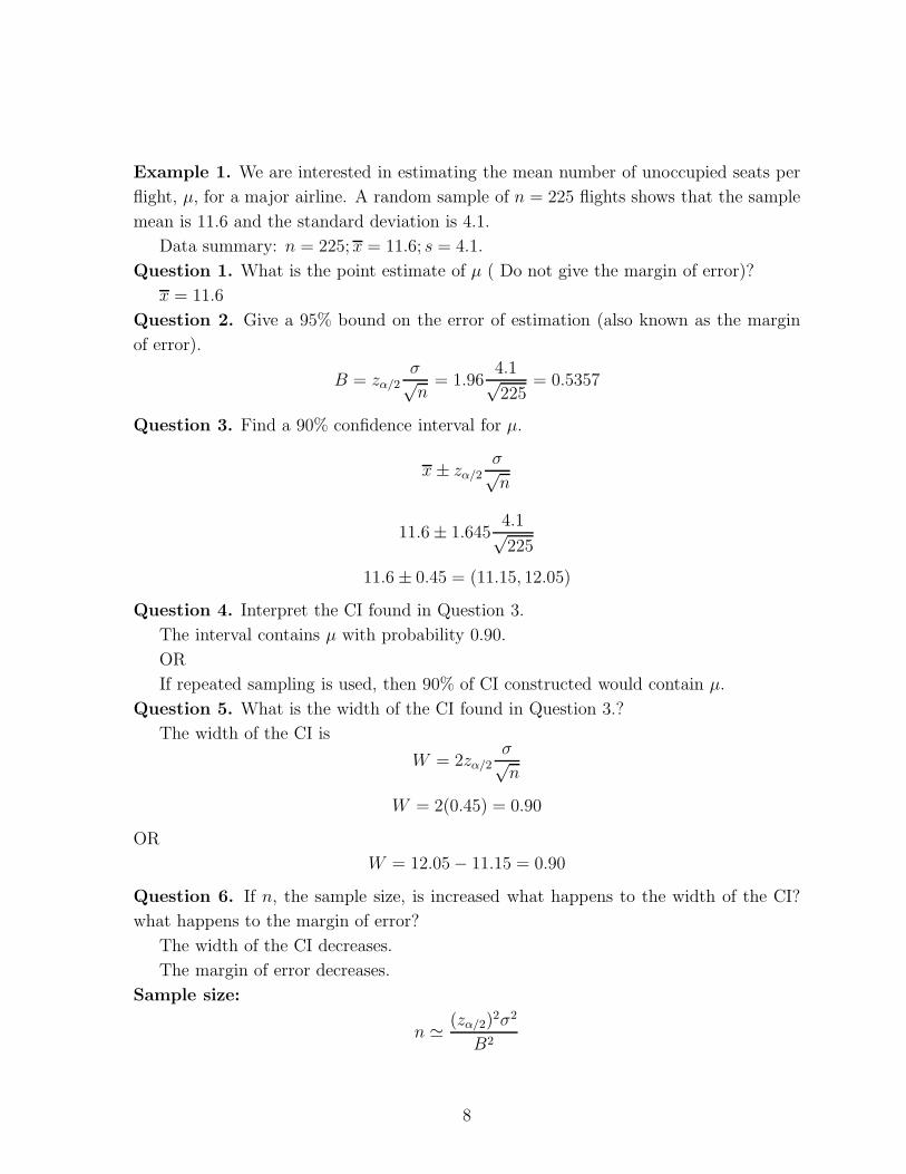
Example 1. We are interested in estimating the mean number of unoccupied seats per
flight, µ, for a major airline. A random sample of n = 225 flights shows that the sample
mean is 11.6 and the standard deviation is 4.1.
Data summary: n = 225; x = 11.6; s = 4.1.
Question 1. What is the point estimate of µ ( Do not give the margin of error)?
x = 11.6
Question 2. Give a 95% bound on the error of estimation (also known as the margin
of error).
B = zα/2σ√n= 1.96
4.1√225
= 0.5357
Question 3. Find a 90% confidence interval for µ.
x± zα/2σ√n
11.6± 1.6454.1√225
11.6± 0.45 = (11.15, 12.05)
Question 4. Interpret the CI found in Question 3.
The interval contains µ with probability 0.90.
OR
If repeated sampling is used, then 90% of CI constructed would contain µ.
Question 5. What is the width of the CI found in Question 3.?
The width of the CI is
W = 2zα/2σ√n
W = 2(0.45) = 0.90
OR
W = 12.05− 11.15 = 0.90
Question 6. If n, the sample size, is increased what happens to the width of the CI?
what happens to the margin of error?
The width of the CI decreases.
The margin of error decreases.
Sample size:
n � (zα/2)2σ2
B2
8

where σ is estimated by s.
Note: In the absence of data, σ is sometimes approximated by R4
where R is the
range.
Example 2. Suppose you want to construct a 99% CI for µ so that W = 0.05. You are
told that preliminary data shows a range from 13.3 to 13.7. What sample size should
you choose?
A. Data summary: α = .01;R = 13.7− 13.3 = .4;
so σ � .4/4 = .1. Now
B = W/2 = 0.05/2 = 0.025. Therefore
n � (zα/2)2σ2
B2
=2.582(.1)2
0.0252= 106.50 .
So n = 107. (round up)
Exercise 1. Find the sample size necessary to reduce W in the flight example to .6. Use
α = 0.05.
4 Single Binomial Population
Parameter of interest: p
Sample data: n, x, p = xn(x here is the number of successes).
Other information: α
Point estimator: p
Estimator mean: µp = p
Standard error: σp =√
pqn
Confidence Interval (C.I.) for p:
p± zα/2
√pq
n
Confidence level: (1 − α)100% which is the probability that the interval estimator
contains the parameter.
Margin of Error.
B = zα/2
√pq
n
9

Assumptions.
1. Large sample (np ≥ 5;nq ≥ 5)
2. Sample is randomly selected
Example 3. A random sample of n = 484 voters in a community produced x = 257
voters in favor of candidate A.
Data summary: n = 484; x = 257; p = xn= 257
484= 0.531.
Question 1. Do we have a large sample size?
np = 484(0.531) = 257 which is ≥ 5.
nq = 484(0.469) = 227 which is ≥ 5.
Therefore we have a large sample size.
Question 2. What is the point estimate of p and its margin of error?
p =x
n=
257
484= 0.531
B = zα/2
√pq
n= 1.96
√(0.531)(0.469)
484= 0.044
Question 3. Find a 90% confidence interval for p.
p± zα/2
√pq
n
0.531± 1.645
√(0.531)(0.469)
484
0.531± 0.037 = (0.494, 0.568)
Question 4. What is the width of the CI found in Question 3.?
The width of the CI is
W = 2zα/2
√pq
n= 2(0.037) = 0.074
Question 5. Interpret the CI found in Question 3.
The interval contains p with probability 0.90.
OR
If repeated sampling is used, then 90% of CI constructed would contain p.
Question 6. If n, the sample size, is increased what happens to the width of the CI?
what happens to the margin of error?
10

The width of the CI decreases.
The margin of error decreases.
Sample size.
n � (zα/2)2(pq)
B2.
Note: In the absence of data, choose p = q = 0.5 or simply pq = 0.25.
Example 4. Suppose you want to provide an accurate estimate of customers preferring
one brand of coffee over another. You need to construct a 95% CI for p so that B = 0.015.
You are told that preliminary data shows a p = 0.35. What sample size should you choose
? Use α = 0.05.
Data summary: α = .05; p = 0.35;B = 0.015
n � (zα/2)2(pq)
B2
=(1.96)2(0.35)(0.65)
0.0152= 3, 884.28
So n = 3, 885. (round up)
Exercise 2. Suppose that no preliminary estimate of p is available. Find the new sample
size. Use α = 0.05.
Exercise 3. Suppose that no preliminary estimate of p is available. Find the sample
size necessary so that α = 0.01.
5 Two Quantitative Populations
Parameter of interest: µ1 − µ2
Sample data:
Sample 1: n1, x1, s1
Sample 2: n2, x2, s2
Point estimator: X1 −X2
Estimator mean: µX1−X2= µ1 − µ2
Standard error: SE(X1 −X2) =
√σ21
n1+
σ22
n2
Confidence Interval.
(x1 − x2)± zα/2
√σ2
1
n1+
σ22
n2
11

Assumptions.
1. Large samples ( n1 ≥ 30;n2 ≥ 30)
2. Samples are randomly selected
3. Samples are independent
Sample size.
n � (zα/2)2(σ2
1 + σ22)
B2
6 Two Binomial Populations
Parameter of interest: p1 − p2
Sample 1: n1, x1, p1 = x1
n1
Sample 2: n2, x2, p2 = x2
n2
p1 − p2 (unknown parameter)
α (significance level)
Point estimator: p1 − p2
Estimator mean: µp1−p2 = p1 − p2
Estimated standard error: σp1−p2 =√
p1q1
n1+ p2q2
n2
Confidence Interval.
(p1 − p2)± zα/2
√p1q1
n1+
p2q2
n2
Assumptions.
1. Large samples,
(n1p1 ≥ 5, n1q1 ≥ 5, n2p2 ≥ 5, n2q2 ≥ 5)
2. Samples are randomly and independently selected
Sample size.
n � (zα/2)2(p1q1 + p2q2)
B2
For unkown parameters:
n � (zα/2)2(0.5)
B2
Review Exercises: Large-Sample Estimation
12

Please show all work. No credit for a correct final answer without a valid argu-
ment. Use the formula, substitution, answer method whenever possible. Show your work
graphically in all relevant questions.
1. A random sample of size n = 100 is selected form a quantitative population. The
data produced a mean and standard deviation of x = 75 and s = 6 respectively.
(i) Estimate the population mean µ, and give a 95% bound on the error of estimation
(or margin of error). (Answer: B=1.18)
(ii) Find a 99% confidence interval for the population mean. (Answer: B=1.55)
(iii) Interpret the confidence interval found in (ii).
(iv) Find the sample size necessary to reduce the width of the confidence interval in
(ii) by half. (Answer: n=400)
2. An examination of the yearly premiums for a random sample of 80 automobile
insurance policies from a major company showed an average of $329 and a standard
deviation of $49.
(i) Give the point estimate of the population parameter µ and a 99% bound on the
error of estimation. (Margin of error). (Answer: B=14.135)
(ii) Construct a 99% confidence interval for µ.
(iii) Suppose we wish our estimate in (i) to be accurate to within $5 with 95% con-
fidence; how many insurance policies should be sampled to achieve the desired level of
accuracy? (Answer: n=369)
3. Suppose we wish to estimate the average daily yield of a chemical manufactured
in a chemical plant. The daily yield recorded for n = 100 days, produces a mean and
standard deviation of x = 870 and s = 20 tons respectively.
(i) Estimate the average daily yield µ, and give a 95% bound on the error of estimation
(or margin of error).
(ii) Find a 99% confidence interval for the population mean.
(iii) Interpret the confidence interval found in (ii).
(iv) Find the sample size necessary to reduce the width of the confidence interval in
(ii) by half.
4. Answer by True of False . (Circle your choice).
T F (i) If the population variance increases and other factors are the same, the width
of the confidence interval for the population mean tends to increase.
13

T F (ii) As the sample size increases, the width of the confidence interval for the
population mean tends to decrease.
T F (iii) Populations are characterized by numerical descriptive measures called sta-
tistics.
T F (iv) If, for a given C.I., α is increased, then the margin of error will increase.
T F (v) The sample standard deviation s can be used to approximate σ when n is
larger than 30.
T F (vi) The sample mean always lies above the population mean.
14

Chapter 3
Large-Sample Tests of Hypothesis
Contents.
1. Elements of a statistical test
2. A Large-sample statistical test
3. Testing a population mean
4. Testing a population proportion
5. Testing the difference between two population means
6. Testing the difference between two population proportions
7. Reporting results of statistical tests: p-Value
1 Elements of a Statistical Test
Null hypothesis: H0
Alternative (research) hypothesis: Ha
Test statistic:
Rejection region : reject H0 if .....
Graph:
Decision: either “Reject H0” or “Do no reject H0”
Conclusion: At 100α% significance level there is (in)sufficient statistical evidence to
“ favor Ha” .
Comments:
* H0 represents the status-quo
* Ha is the hypothesis that we want to provide evidence to justify. We show that Ha
is true by showing that H0 is false, that is proof by contradiction.
Type I error ≡ { reject H0|H0 is true }
15

Type II error ≡ { do not reject H0|H0 is false}α = Prob{Type I error}β = Prob{Type II error}Power of a statistical test:
Prob{reject H0 — H0 is false }= 1− β
Example 1.
H0: Innocent
Ha: Guilty
α = Prob{sending an innocent person to jail}β = Prob{letting a guilty person go free}
Example 2.
H0: New drug is not acceptable
Ha: New drug is acceptable
α = Prob{marketing a bad drug}β = Prob{not marketing an acceptable drug}
2 A Large-Sample Statistical Test
Parameter of interest: θ
Sample data: n, θ, σθ
Test:
Null hypothesis (H0) : θ = θ0
Alternative hypothesis (Ha): 1) θ > θ0; 2) θ < θ0; 3) θ = θ0
Test statistic (TS):
z =θ − θ0
σθ
Critical value: either zα or zα/2
Rejection region (RR) :
1) Reject H0 if z > zα
2) Reject H0 if z < −zα
3) Reject H0 if z > zα/2 or z < −zα/2
Graph:
Decision: 1) if observed value is in RR: “Reject H0”
2) if observed value is not in RR: “Do no reject H0”
16

Conclusion: At 100α% significance level there is (in)sufficient statistical evidence to
· · · .Assumptions: Large sample + others (to be specified in each case).
One tailed statistical test
Upper (right) tailed test
Lower (left) tailed test
Two tailed statistical test
3 Testing a Population Mean
Parameter of interest: µ
Sample data: n, x, s
Other information: µ0= target value, α
Test:
H0 : µ = µ0
Ha : 1) µ > µ0; 2) µ < µ0; 3) µ = µ0
T.S. :
z =x− µ0
σ/√n
Rejection region (RR) :
1) Reject H0 if z > zα
2) Reject H0 if z < −zα
3) Reject H0 if z > zα/2 or z < −zα/2
Graph:
Decision: 1) if observed value is in RR: “Reject H0”
2) if observed value is not in RR: “Do no reject H0”
Conclusion: At 100α% significance level there is (in)sufficient statistical evidence to
“ favor Ha” .
Assumptions:
Large sample (n ≥ 30)
Sample is randomly selected
Example: Test the hypothesis that weight loss in a new diet program exceeds 20 pounds
during the first month.
Sample data : n = 36, x = 21, s2 = 25, µ0 = 20, α = 0.05
H0 : µ = 20 (µ is not larger than 20)
17

Ha : µ > 20 (µ is larger than 20)
T.S. :
z =x− µ0
s/√n
=21− 20
5/√36
= 1.2
Critical value: zα = 1.645
RR: Reject H0 if z > 1.645
Graph:
Decision: Do not reject H0
Conclusion: At 5% significance level there is insufficient statistical evidence to con-
clude that weight loss in a new diet program exceeds 20 pounds per first month.
Exercise: Test the claim that weight loss is not equal to 19.5.
4 Testing a Population Proportion
Parameter of interest: p (unknown parameter)
Sample data: n and x (or p = xn)
p0 = target value
α (significance level)
Test:
H0 : p = p0
Ha: 1) p > p0; 2) p < p0; 3) p = p0
T.S. :
z =p− p0√p0q0/n
RR:
1) Reject H0 if z > zα
2) Reject H0 if z < −zα
3) Reject H0 if z > zα/2 or z < −zα/2
Graph:
Decision:
1) if observed value is in RR: “Reject H0”
2) if observed value is not in RR: “Do not reject H0”
Conclusion: At (α)100% significance level there is (in)sufficient statistical evidence
to “ favor Ha” .
Assumptions:
18

1. Large sample (np ≥ 5, nq ≥ 5)
2. Sample is randomly selected
Example. Test the hypothesis that p > .10 for sample data: n = 200, x = 26.
Solution.
p = xn= 26
200= .13,
Now
H0 : p = .10
Ha : p > .10
TS:
z =p− p0√p0q0/n
=.13− .10√
(.10)(.90)/200= 1.41
RR: reject H0 if z > 1.645
Graph:
Dec: Do not reject H0
Conclusion: At 5% significance level there is insufficient statistical evidence to con-
clude that p > .10.
Exercise Is the large sample assumption satisfied here ?
5 Comparing Two Population Means
Parameter of interest: µ1 − µ2
Sample data:
Sample 1: n1, x1, s1
Sample 2: n2, x2, s2
Test:
H0 : µ1 − µ2 = D0
Ha : 1)µ1 − µ2 > D0; 2) µ1 − µ2 < D0;
3) µ1 − µ2 = D0
T.S. :
z =(x1 − x2)−D0√
σ21
n1+
σ22
n2
RR:
1) Reject H0 if z > zα
2) Reject H0 if z < −zα
19

3) Reject H0 if z > zα/2 or z < −zα/2
Graph:
Decision:
Conclusion:
Assumptions:
1. Large samples ( n1 ≥ 30;n2 ≥ 30)
2. Samples are randomly selected
3. Samples are independent
Example: (Comparing two weight loss programs)
Refer to the weight loss example. Test the hypothesis that weight loss in the two diet
programs are different.
1. Sample 1 : n1 = 36, x1 = 21, s21 = 25 (old)
2. Sample 2 : n2 = 36, x2 = 18.5, s22 = 24 (new)
D0 = 0, α = 0.05
H0 : µ1 − µ2 = 0
Ha : µ1 − µ2 = 0,
T.S. :
z =(x1 − x2)− 0√
σ21
n1+
σ22
n2
= 2.14
Critical value: zα/2 = 1.96
RR: Reject H0 if z > 1.96 or z < −1.96
Graph:
Decision: Reject H0
Conclusion: At 5% significance level there is sufficient statistical evidence to conclude
that weight loss in the two diet programs are different.
Exercise: Test the hypothesis that weight loss in the old diet program exceeds that of
the new program.
Exercise: Test the claim that the difference in mean weight loss for the two programs
is greater than 1.
6 Comparing Two Population Proportions
Parameter of interest: p1 − p2
Sample 1: n1, x1, p1 = x1
n1,
20

Sample 2: n2, x2, p2 = x2
n2,
p1 − p2 (unknown parameter)
Common estimate:
p =x1 + x2
n1 + n2
Test:
H0 : p1 − p2 = 0
Ha : 1) p1 − p2 > 0
2) p1 − p2 < 0
3) p1 − p2 = 0
T.S. :
z =(p1 − p2)− 0√pq(1/n1 + 1/n2)
RR:
1) Reject H0 if z > zα
2) Reject H0 if z < −zα
3) Reject H0 if z > zα/2 or z < −zα/2
Graph:
Decision:
Conclusion:
Assumptions:
Large sample(n1p1 ≥ 5, n1q1 ≥ 5, n2p2 ≥ 5, n2q2 ≥ 5)
Samples are randomly and independently selected
Example: Test the hypothesis that p1 − p2 < 0 if it is known that the test statistic is
z = −1.91.
Solution:
H0 : p1 − p2 = 0
Ha : p1 − p2 < 0
TS: z = −1.91
RR: reject H0 if z < −1.645
Graph:
Dec: reject H0
Conclusion: At 5% significance level there is sufficient statistical evidence to conclude
that p1 − p2 < 0.
21

Exercise: Repeat as a two tailed test
7 Reporting Results of Statistical Tests: P-Value
Definition. The p-value for a test of a hypothesis is the smallest value of α for which
the null hypothesis is rejected, i.e. the statistical results are significant.
The p-value is called the observed significance level
Note: The p-value is the probability ( when H0 is true) of obtaining a value of the
test statistic as extreme or more extreme than the actual sample value in support of Ha.
Examples. Find the p-value in each case:
(i) Upper tailed test:
H0 : θ = θ0
Ha : θ > θ0
TS: z = 1.76
p-value = .0392
(ii) Lower tailed test:
H0 : θ = θ0
Ha : θ < θ0
TS: z = −1.86
p-value = .0314
(iii) Two tailed test:
H0 : θ = θ0
Ha : θ = θ0
TS: z = 1.76
p-value = 2(.0392) = .0784
Decision rule using p-value: (Important)
Reject H0 for all α > p− value
Review Exercises: Testing Hypothesis
Please show all work. No credit for a correct final answer without a valid argu-
ment. Use the formula, substitution, answer method whenever possible. Show your work
graphically in all relevant questions.
1. A local pizza parlor advertises that their average time for delivery of a pizza is
within 30 minutes of receipt of the order. The delivery time for a random sample of 64
22

orders were recorded, with a sample mean of 34 minutes and a standard deviation of 21
minutes.
(i) Is there sufficient evidence to conclude that the actual delivery time is larger than
what is claimed by the pizza parlor? Use α = .05.
H0:
Ha:
T.S. (Answer: 1.52)
R.R.
Graph:
Dec:
Conclusion:
((ii) Test the hypothesis that Ha : µ = 30.
2. Answer by True of False . (Circle your choice).
T F (v) If, for a given test, α is fixed and the sample size is increased, then β will
increase.
23

Chapter 4
Small-Sample Tests of Hypothesis
Contents:
1. Introduction
2. Student’s t distribution
3. Small-sample inferences about a population mean
4. Small-sample inferences about the difference between two means: Independent
Samples
5. Small-sample inferences about the difference between two means: Paired Samples
6. Inferences about a population variance
7. Comparing two population variances
1 Introduction
When the sample size is small we only deal with normal populations.
For non-normal (e.g. binomial) populations different techniques are necessary
2 Student’s t Distribution
RECALL
For small samples (n < 30) from normal populations, we have
z =x− µ
σ/√n
If σ is unknown, we use s instead; but we no more have a Z distribution
Assumptions.
24

1. Sampled population is normal
2. Small random sample (n < 30)
3. σ is unknown
t =x− µ
s/√n
Properties of the t Distribution:
(i) It has n− 1 degrees of freedom (df)
(ii) Like the normal distribution it has a symmetric mound-shaped probability distri-
bution
(iii) More variable (flat) than the normal distribution
(iv) The distribution depends on the degrees of freedom. Moreover, as n becomes
larger, t converges to Z.
(v) Critical values (tail probabilities) are obtained from the t table
Examples.
(i) Find t0.05,5 = 2.015
(ii) Find t0.005,8 = 3.355
(iii) Find t0.025,26 = 2.056
3 Small-Sample Inferences About a PopulationMean
Parameter of interest: µ
Sample data: n, x, s
Other information: µ0= target value, α
Point estimator: x
Estimator mean: µx = µ
Estimated standard error: σx = s/√n
Confidence Interval for µ:
x± tα2
,n−1(s√n)
Test:
H0 : µ = µ0
Ha : 1) µ > µ0; 2) µ < µ0; 3) µ = µ0.
Critical value: either tα,n−1 or tα2
,n−1
25

T.S. : t = x−µ0
s/√
n
RR:
1) Reject H0 if t > tα,n−1
2) Reject H0 if t < −tα,n−1
3) Reject H0 if t > tα2
,n−1 or t < −tα2
,n−1
Graph:
Decision: 1) if observed value is in RR: “Reject H0”
2) if observed value is not in RR: “Do not reject H0”
Conclusion: At 100α% significance level there is (in)sufficient statistical evidence to
“favor Ha” .
Assumptions.
1. Small sample (n < 30)
2. Sample is randomly selected
3. Normal population
4. Unknown variance
Example For the sample data given below, test the hypothesis that weight loss in a new
diet program exceeds 20 pounds per first month.
1. Sample data: n = 25, x = 21.3, s2 = 25, µ0 = 20, α = 0.05
Critical value: t0.05,24 = 1.711
H0 : µ = 20
Ha : µ > 20,
T.S.:
t =x− µ0
s/√n
=21.3− 20
5/√25
= 1.3
RR: Reject H0 if t > 1.711
Graph:
Decision: Do not reject H0
Conclusion: At 5% significance level there is insufficient statistical evidence to con-
clude that weight loss in a new diet program exceeds 20 pounds per first month.
Exercise. Test the claim that weight loss is not equal to 19.5, (i.e. Ha : µ = 19.5).
4 Small-Sample Inferences About the Difference Be-
tween Two Means: Independent Samples
Parameter of interest: µ1 − µ2
26

Sample data:
Sample 1: n1, x1, s1
Sample 2: n2, x2, s2
Other information: D0= target value, α
Point estimator: X1 −X2
Estimator mean: µX1−X2= µ1 − µ2
Assumptions.
1. Normal populations
2. Small samples ( n1 < 30;n2 < 30)
3. Samples are randomly selected
4. Samples are independent
5. Variances are equal with common variance
σ2 = σ21 = σ2
2
Pooled estimator for σ.
s =
√(n1 − 1)s2
1 + (n2 − 1)s22
n1 + n2 − 2
Estimator standard error:
σX1−X2= σ
√1
n1+
1
n2
Reason:
σX1−X2=
√σ2
1
n1
+σ2
2
n2
=
√σ2
n1
+σ2
n2
= σ
√1
n1+
1
n2
Confidence Interval:
(x1 − x2)± (tα/2,n1+n2−2)(s
√1
n1+
1
n2)
Test:
H0 : µ1 − µ2 = D0
27

Ha : 1)µ1 − µ2 > D0; 2) µ1 − µ2 < D0;
3) µ1 − µ2 = D0
T.S. :
t =(x1 − x2)−D0
s√
1n1
+ 1n2
RR: 1) Reject H0 if t > tα,n1+n2−2
2) Reject H0 if t < −tα,n1+n2−2
3) Reject H0 if t > tα/2,n1+n2−2 or t < −tα/2,n1+n2−2
Graph:
Decision:
Conclusion:
Example.(Comparison of two weight loss programs)
Refer to the weight loss example. Test the hypothesis that weight loss in a new diet
program is different from that of an old program. We are told that that the observed
value is 2.2 and the we know that
1. Sample 1 : n1 = 7
2. Sample 2 : n2 = 8
α = 0.05
Solution.
H0 : µ1 − µ2 = 0
Ha : µ1 − µ2 = 0
T.S. :
t =(x1 − x2)− 0
s√
1n1
+ 1n2
= 2.2
Critical value: t.025,13 = 2.160
RR: Reject H0 if t > 2.160 or t < −2.160
Graph:
Decision: Reject H0
Conclusion: At 5% significance level there is sufficient statistical evidence to conclude
that weight loss in the two diet programs are different.
Exercise: Test the claim that the difference in mean weight loss for the two programs
is greater than 0.
Minitab Commands: A twosample t procedure with a pooled estimate of variance
MTB> twosample C1 C2;
SUBC>pooled;
28

SUBC> alternative 1.
Note: alternative : 1=right-tailed; -1=left tailed; 0=two tailed.
5 Small-Sample Inferences About the Difference Be-
tween Two Means: Paired Samples
Parameter of interest: µ1 − µ2 = µd
Sample of paired differences data:
Sample : n = number of pairs, d = sample mean, sd
Other information: D0= target value, α
Point estimator: d
Estimator mean: µd = µd
Assumptions.
1. Normal populations
2. Small samples ( n1 < 30;n2 < 30)
3. Samples are randomly selected
4. Samples are paired (not independent)
Sample standard deviation of the sample of n paired differences
sd =
√∑ni=1(di − d)2
n− 1
Estimator standard error: σd = sd/√n
Confidence Interval.
d± tα/2,n−1sd/√n
Test.
H0 : µ1 − µ2 = D0 (equivalently, µd = D0)
Ha : 1)µ1 − µ2 = µd > D0; 2) µ1 − µ2 = µd < D0;
3) µ1 − µ2 = µd = D0,
T.S. :
t =d−D0
sd/√n
RR:
1) Reject H0 if t > tα,n−1
2) Reject H0 if t < −tα,n−1
29

3) Reject H0 if t > tα/2,n−1 or t < −tα/2,n−1
Graph:
Decision:
Conclusion:
Example. A manufacturer wishes to compare wearing qualities of two different types
of tires, A and B. For the comparison a tire of type A and one of type B are randomly
assigned and mounted on the rear wheels of each of five automobiles. The automobiles
are then operated for a specified number of miles, and the amount of wear is recorded
for each tire. These measurements are tabulated below.
Automobile Tire A Tire B1 10.6 10.22 9.8 9.43 12.3 11.84 9.7 9.15 8.8 8.3
x1 = 10.24 x2 = 9.76
Using the previous section test we would have t = 0.57 resulting in an insignificant
test which is inconsistent with the data.
Automobile Tire A Tire B d=A-B1 10.6 10.2 .42 9.8 9.4 .43 12.3 11.8 .54 9.7 9.1 .65 8.8 8.3 .5
x1 = 10.24 x2 = 9.76 d = .48
Q1: Provide a summary of the data in the above table.
Sample summary: n = 5, d = .48, sd = .0837
Q2: Do the data provide sufficient evidence to indicate a difference in average wear
for the two tire types.
Test. (parameter µd = µ1 − µ2)
H0 : µd = 0
Ha : µd = 0
T.S. :
t =d−D0
sd/√n
=.48− 0
.0837/√5= 12.8
30

RR: Reject H0 if t > 2.776 or t < −2.776 ( t.025,4 = 2.776)
Graph:
Decision: Reject H0
Conclusion: At 5% significance level there is sufficient statistical evidence to to con-
clude that the average amount of wear for type A tire is different from that for type B
tire.
Exercise. Construct a 99% confidence interval for the difference in average wear for the
two tire types.
6 Inferences About a Population Variance
Chi-square distribution. When a random sample of size n is drawn from a normal
population with mean µ and standard deviation σ, the sampling distribution of S2 de-
pends on n. The standardized distribution of S2 is called the chi-square distribution and
is given by
X 2 =(n− 1)s2
σ2
Degrees of freedom (df): ν = n− 1
Graph: Non-symmetrical and depends on df
Critical values: using X 2 tables
Test.
H0 : σ2 = σ20
Ha : σ2 = σ20 (two-tailed test).
T.S. :
X 2 =(n− 1)s2
σ20
RR: Reject H0 if X 2 > X 2α/2 or X 2 < X 2
1−α/2 where X 2 is based on (n− 1) degrees of
freedom.
Graph:
Decision:
Conclusion:
Assumptions.
1. Normal population
2. Random sample
Example:
31

Use text
7 Comparing Two Population Variances
F-distribution. When independent samples are drawn from two normal populations
with equal variances then S21/S
22 possesses a sampling distribution that is known as an
F distribution. That is
F =s21
s22
Degrees of freedom (df): ν1 = n1 − 1; ν2 = n2 − 1
Graph: Non-symmetrical and depends on df
Critical values: using F tables
Test.
H0 : σ21 = σ2
2
Ha : σ21 = σ2
2 (two-tailed test).
T.S. :F =s21
s22where s2
1 is the larger sample variance.
Note: F = larger sample variancesmaller sample variance
RR: Reject H0 if F > Fα/2 where Fα/2 is based on (n1 − 1) and (n2 − 1) degrees of
freedom.
Graph:
Decision:
Conclusion:
Assumptions.
1. Normal populations
2. Independent random samples
Example. (Investment Risk) Investment risk is generally measured by the volatility
of possible outcomes of the investment. The most common method for measuring in-
vestment volatility is by computing the variance ( or standard deviation) of possible
outcomes. Returns over the past 10 years for first alternative and 8 years for the second
alternative produced the following data:
Data Summary:
Investment 1: n1 = 10, x1 = 17.8%; s21 = 3.21
Investment 2: n2 = 8, x2 = 17.8%; s22 = 7.14
Both populations are assumed to be normally distributed.
32

Q1: Do the data present sufficient evidence to indicate that the risks for investments
1 and 2 are unequal ?
Solution.
Test:
H0 : σ21 = σ2
2
Ha : σ21 = σ2
2 (two-tailed test).
T.S. :
F =s22
s21
=7.14
3.21= 2.22
.
RR: Reject H0 if F > Fα/2 where
Fα/2,n2−1,n1−1 = F.025,7,9 = 4.20
Graph:
Decision: Do not reject H0
Conclusion: At 5% significance level there is insufficient statistical evidence to indicate
that the risks for investments 1 and 2 are unequal.
Exercise. Do the upper tail test. That is Ha : σ21 > σ2
2 .
33

Chapter 5
Analysis of Variance
Contents.
1. Introduction
2. One Way ANOVA: Completely Randomized Experimental Design
3. The Randomized Block Design
1 Introduction
Analysis of variance is a statistical technique used to compare more than two popu-
lation means by isolating the sources of variability.
Example. Four groups of sales people for a magazine sales agency were subjected to
different sales training programs. Because there were some dropouts during the training
program, the number of trainees varied from program to program. At the end of the
training programs each salesperson was assigned a sales area from a group of sales areas
that were judged to have equivalent sales potentials. The table below lists the number
of sales made by each person in each of the four groups of sales people during the first
week after completing the training program. Do the data present sufficient evidence to
indicate a difference in the mean achievement for the four training programs?
Goal. Test whether the means are equal or not. That is
H0 : µ1 = µ2 = µ3 = µ4
Ha : Not all means are equal
Definitions:
(i) Response: variable of interest or dependent variable (sales)
(ii) Factor: categorical variable or independent variable (training technique)
(iii) Treatment levels (factor levels): method of training; t =4
34
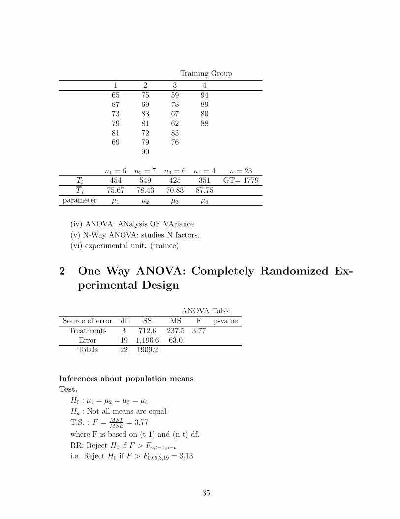
Training Group
1 2 3 465 75 59 9487 69 78 8973 83 67 8079 81 62 8881 72 8369 79 76
90
n1 = 6 n2 = 7 n3 = 6 n4 = 4 n = 23Ti 454 549 425 351 GT= 1779
T i 75.67 78.43 70.83 87.75parameter µ1 µ2 µ3 µ4
(iv) ANOVA: ANalysis OF VAriance
(v) N-Way ANOVA: studies N factors.
(vi) experimental unit: (trainee)
2 One Way ANOVA: Completely Randomized Ex-
perimental Design
ANOVA Table
Source of error df SS MS F p-valueTreatments 3 712.6 237.5 3.77
Error 19 1,196.6 63.0Totals 22 1909.2
Inferences about population means
Test.
H0 : µ1 = µ2 = µ3 = µ4
Ha : Not all means are equal
T.S. : F = MSTMSE
= 3.77
where F is based on (t-1) and (n-t) df.
RR: Reject H0 if F > Fα,t−1,n−t
i.e. Reject H0 if F > F0.05,3,19 = 3.13
35

Graph:
Decision: Reject H0
Conclusion: At 5% significance level there is sufficient statistical evidence to indicate
a difference in the mean achievement for the four training programs.
Assumptions.
1. Sampled populations are normal
2. Independent random samples
3. All t populations have equal variances
Computations.
ANOVA Table
S of error df SS MS F p-valueTrments t-1 SST MST=SST/(t-1) MST/MSEError n-t SSE MSE=SSE/(n-t)Totals n-1 TSS
Training Group
1 2 3 4x11 x21 x31 x41
x12 x22 x32 x42
x13 x23 x33 x43
x14 x24 x34 x44
x15 x25 x35
x16 x26 x36
x27
n1 n2 n3 n4 nTi T1 T2 T3 T4 GTT i T 1 T 2 T 3 T 4
parameter µ1 µ2 µ3 µ4
Notation:
TSS: sum of squares of total deviation.
SST: sum of squares of total deviation between treatments.
SSE: sum of squares of total deviation within treatments (error).
CM: correction for the mean
36
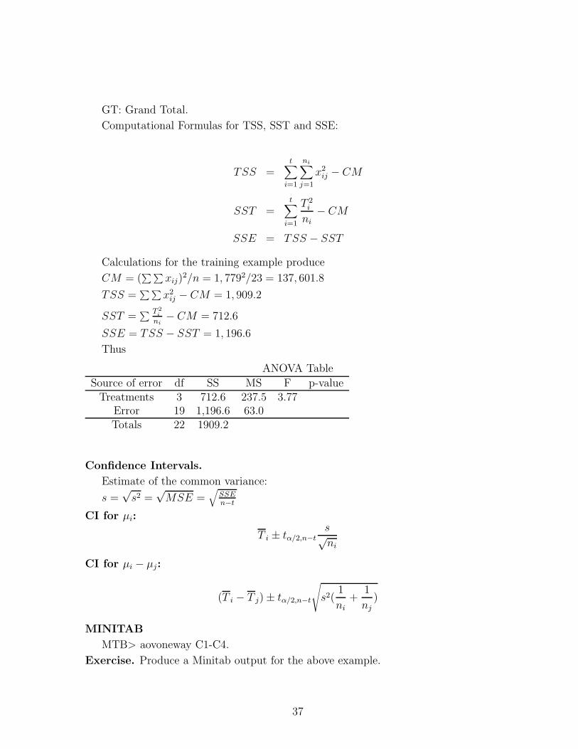
GT: Grand Total.
Computational Formulas for TSS, SST and SSE:
TSS =t∑
i=1
ni∑j=1
x2ij − CM
SST =t∑
i=1
T 2i
ni
− CM
SSE = TSS − SST
Calculations for the training example produce
CM = (∑ ∑
xij)2/n = 1, 7792/23 = 137, 601.8
TSS =∑ ∑
x2ij − CM = 1, 909.2
SST =∑ T 2
i
ni− CM = 712.6
SSE = TSS − SST = 1, 196.6
Thus
ANOVA Table
Source of error df SS MS F p-valueTreatments 3 712.6 237.5 3.77
Error 19 1,196.6 63.0Totals 22 1909.2
Confidence Intervals.
Estimate of the common variance:
s =√s2 =
√MSE =
√SSEn−t
CI for µi:
T i ± tα/2,n−ts√ni
CI for µi − µj:
(T i − T j)± tα/2,n−t
√s2(
1
ni
+1
nj
)
MINITAB
MTB> aovoneway C1-C4.
Exercise. Produce a Minitab output for the above example.
37

3 The Randomized Block Design
Extends paired-difference design to more than two treatments.
A randomized block design consists of b blocks, each containing t experimental units.
The t treatments are randomly assigned to the units in each block, and each treatment
appears once in every block.
Example. A consumer preference study involving three different package designs (treat-
ments) was laid out in a randomized block design among four supermarkets (blocks).
The data shown in Table 1. below represent the number of units sold for each package
design within each supermarket during each of three given weeks.
(i) Provide a data summary.
(ii) Do the data present sufficient evidence to indicate a difference in the mean sales
for each package design (treatment)?
(iii) Do the data present sufficient evidence to indicate a difference in the mean sales
for the supermarkets?
weeks
w1 w2 w3s1 (1) 17 (3) 23 (2) 34s2 (3) 21 (1) 15 (2) 26s3 (1) 1 (2) 23 (3) 8s4 (2) 22 (1) 6 (3) 16
Remarks.
(i) In each supermarket (block) the first entry represents the design (treatment) and
the second entry represents the sales per week.
(ii) The three designs are assigned to each supermarket completely at random.
(iii) An alternate design would be to use 12 supermarkets. Each design (treatment)
would be randomly assigned to 4 supermarkets. In this case the difference in sales could
be due to more than just differences in package design. That is larger supermarkets
would be expected to have larger overall sales of the product than smaller supermarkets.
The randomized block design eliminates the store-to-store variability.
For computational purposes we rearrange the data so that
Data Summary. The treatment and block totals are
t = 3 treatments; b = 4 blocks
38

Treatments
t1 t2 t3 Bi
s1 17 34 23 B1
s2 15 26 21 B2
s3 1 23 8 B3
s4 6 22 16 B4
Ti T1 T2 T3
T1 = 39, T2 = 105, T3 = 68
B1 = 74, B2 = 62, B3 = 32, B4 = 44
Calculations for the training example produce
CM = (∑ ∑
xij)2/n = 3, 745.33
TSS =∑ ∑
x2ij − CM = 940.67
SST =∑ T 2
i
b− CM = 547.17
SSB =∑ B2
i
t− CM = 348.00
SSE = TSS − SST − SSB = 45.50
39

MINITAB.(Commands and Printouts)
MTB> Print C1-C3
ROW UNITS TRTS BLOCKS
1 17 1 12 34 2 13 23 3 14 15 1 25 26 2 26 21 3 27 1 1 38 23 2 39 8 3 310 6 1 411 22 2 412 16 3 4
MTB> ANOVA C1=C2 C3
ANOVA Table
Source of error df SS MS F p-valueTreatments 2 547.17 273.58 36.08 0.000
Blocks 3 348.00 116.00 15.30 0.003Error 6 45.50 7.58Totals 11 940.67
40

Solution to (ii)
Test.
H0 : µ1 = µ2 = µ3
Ha : Not all means are equal
T.S. : F = MSTMSE
= 36.09
where F is based on (t-1) and (n-t-b+1) df.
RR: Reject H0 if F > Fα,t−1,n−t−b+1
i.e. Reject H0 if F > F0.05,2,6 = 5.14
Graph:
Decision: Reject H0
Conclusion: At 5% significance level there is sufficient statistical evidence to indicate
a real difference in the mean sales for the three package designs.
Note that n− t− b+ 1 = (t− 1)(b− 1).
Solution to (iii)
Test.
H0 : Block means are equal
Ha : Not all block means are equal (i.e. blocking is desirable)
T.S.: F = MSBMSE
= 15.30
where F is based on (b-1) and (n-t-b+1) df.
RR: Reject H0 if F > Fα,b−1,n−t−b+1
i.e. Reject H0 if F > F0.005,3,6 = 12.92
Graph:
Decision: Reject H0
Conclusion: At .5% significance level there is sufficient statistical evidence to indicate
a real difference in the mean sales for the four supermarkets, that is the data supports
our decision to use supermarkets as blocks.
Assumptions.
1. Sampled populations are normal
2. Dependent random samples due to blocking
3. All t populations have equal variances
Confidence Intervals.
Estimate of the common variance:
s =√s2 =
√MSE =
√SSE
n−t−b+1
CI for µi − µj:
41

(T i − T j)± tα/2,n−t−b+1s
√2
b
Exercise. Construct a 90% C.I. for the difference between mean sales from package
designs 1 and 2.
42

Chapter 6
Simple Linear Regression andCorrelation
Contents.
1. Introduction: Example
2. A Simple Linear probabilistic model
3. Least squares prediction equation
4. Inferences concerning the slope
5. Estimating E(y|x) for a given x
6. Predicting y for a given x
7. Coefficient of correlation
8. Analysis of Variance
9. Computer Printouts
1 Introduction
Linear regression is a statistical technique used to predict (forecast) the value of a
variable from known related variables.
Example.( Ad Sales) Consider the problem of predicting the gross monthly sales volume
y for a corporation that is not subject to substantial seasonal variation in its sales volume.
For the predictor variable x we use the the amount spent by the company on advertising
during the month of interest. We wish to determine whether advertising is worthwhile,
that is whether advertising is actually related to the firm’s sales volume. In addition we
wish to use the amount spent on advertising to predict the sales volume. The data in the
table below represent a sample of advertising expenditures,x, and the associated sales
43
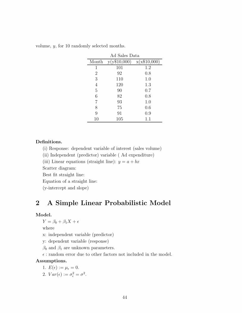
volume, y, for 10 randomly selected months.
Ad Sales Data
Month y(y$10,000) x(x$10,000)1 101 1.22 92 0.83 110 1.04 120 1.35 90 0.76 82 0.87 93 1.08 75 0.69 91 0.910 105 1.1
Definitions.
(i) Response: dependent variable of interest (sales volume)
(ii) Independent (predictor) variable ( Ad expenditure)
(iii) Linear equations (straight line): y = a+ bx
Scatter diagram:
Best fit straight line:
Equation of a straight line:
(y-intercept and slope)
2 A Simple Linear Probabilistic Model
Model.
Y = β0 + β1X + ε
where
x: independent variable (predictor)
y: dependent variable (response)
β0 and β1 are unknown parameters.
ε : random error due to other factors not included in the model.
Assumptions.
1. E(ε) := µε = 0.
2. V ar(ε) := σ2ε = σ2.
44

3. The r.v. ε has a normal distribution with mean 0 and variance σ2.
4. The random components of any two observed y values are independent.
3 Least Squares Prediction Equation
The least squares prediction equation is sometimes called the estimated regression
equation or the prediction equation.
y = β0 + β1x
This equation is obtained by using the method of least squares; that is
min∑
(y − y)2
Computational Formulas.
Objective: Estimate β0, β1 and σ2.
x =∑
x/n; y =∑
y/n
SSxx =∑(x− x)2 =
∑x2 − (
∑x)2/n
SSyy =∑(y − y)2 =
∑y2 − (
∑y)2/n
SSxy =∑(x− x)(y − y) =
∑xy − (
∑x)(
∑y)/n
β1 = SSxy/SSxx
β0 = y − β1x.
To estimate σ2
SSE = SSyy − β1SSxy
= SSyy − (SSxy)2/SSxx .
s2 =SSE
n− 2
Remarks.
(i) β1 : is the slope of the estimated regression equation.
(ii) s2 provides a measure of spread of points (x, y) around the regression line.
Ad Sales example
Question 1. Do a scatter diagram. Can you say that x and y are linearly related?
Answer.
Question 2. Use the computational formulas to provide a data summary.
45

Answer.
Data Summary.
x = 0.94; y = 95.9
SSxx = .444
SSxy = 23.34
SSyy = 1600.9
46

Optional material
Ad Sales Calculations
Month x y x2 xy y2
1 1.2 101 1.44 121.2 10,2012 0.8 92 0.64 73.6 8,4643 1.0 110 1.00 110.0 12,1004 1.3 120 1.69 156.0 14,4005 0.7 90 0.49 63.0 8,1006 0.8 82 0.64 65.6 6,7247 1.0 93 1.00 93.0 8,6498 0.6 75 0.36 45.0 5,6259 0.9 91 0.81 81.9 8,28110 1.1 105 1.21 115.5 11,025Sum
∑x
∑y
∑x2 ∑
xy∑
y2
9.4 959 9.28 924.8 93,569x = 0.94 y = 95.9
x =∑
x/n = 0.94; y =∑
y/n = 95.9
SSxx =∑
x2 − (∑
x)2/n = 9.28− (9.4)2
10= .444
SSxy =∑
xy − (∑
x)(∑
y)/n = 924.8− (9.4)(959)10
= 23.34
SSyy =∑
y2 − (∑
y)2/n = 93, 569− (959)2
10= 1600.9
47

Question 3. Estimate the parameters β0, and β1.
Answer.
β1 = SSxy/SSxx = 23.34.444
= 52.5676 � 52.57
β0 = y − β1x = 95.9− (52.5676)(.94) � 46.49.
Question 4. Estimate σ2.
Answer.
SSE = SSyy − β1SSxy
= 1, 600.9− (52.5676)(23.34) = 373.97 .
Therefore
s2 =SSE
n− 2=
373.97
8= 46.75
Question 5. Find the least squares line for the data.
Answer.
y = β0 + β1x = 46.49 + 52.57x
Remark. This equation is also called the estimated regression equation or prediction
line.
Question 6. Predict sales volume, y, for a given expenditure level of $10, 000 (i.e.
x = 1.0).
Answer.
y = 46.49 + 52.57x = 46.49 + (52.57)(1.0) = 99.06.
So sales volume is $990, 600.
Question 7. Predict the mean sales volume E(y|x) for a given expenditure level of
$10, 000, x = 1.0.
Answer.
E(y|x) = 46.49 + 52.57x = 46.49 + (52.57)(1.0) = 99.06
so the mean sales volume is $990, 600.
Remark. In Question 6 and Question 7 we obtained the same estimate, the bound
on the error of estimation will, however, be different.
4 Inferences Concerning the Slope
Parameter of interest: β1
Point estimator: β1
48

Estimator mean: µβ1= β1
Estimator standard error: σβ1= σ/
√SSxx
Test.
H0 : β1 = β10 (no linear relationship)
Ha : β1 = β10 (there is linear relationship)
T.S. :
t =β1 − β10
s/√SSxx
RR:
Reject H0 if t > tα/2,n−2 or t < −tα/2,n−2
Graph:
Decision:
Conclusion:
Question 8. Determine whether there is evidence to indicate a linear relationship be-
tween advertising expenditure, x, and sales volume, y.
Answer.
Test.
H0 : β1 = 0 (no linear relationship)
Ha : β1 = 0 (there is linear relationship)
T.S. :
t =β1 − 0
s/√SSxx
=52.57− 0
6.84/√.444
= 5.12
RR: ( critical value: t.025,8 = 2.306)
Reject H0 if t > 2.306 or t < −2.306
Graph:
Decision: Reject H0
Conclusion: At 5% significance level there is sufficient statistical evidence to indicate
a linear relation ship between advertising expenditure, x, and sales volume, y.
Confidence interval for β1:
β1 ± tα/2,n−2s√
SSxx
Question 9. Find a 95% confidence interval for β1.
Answer.
49

β1 ± tα/2,n−2s√
SSxx
52.57± 2.3066.84√.444
52.57± 23.57 = (28.90, 76.24)
5 Estimating E(y|x) For a Given x
The confidence interval (CI) for the expected (mean) value of y given x = xp is given
by
y ± tα/2,n−2
√s2[
1
n+
(xp − x)2
SSxx]
6 Predicting y for a Given x
The prediction interval (PI) for a particular value of y given x = xp is given by
y ± tα/2,n−2
√s2[1 +
1
n+
(xp − x)2
SSxx]
7 Coefficient of Correlation
In a previous section we tested for a linear relationship between x and y.
Now we examine how strong a linear relationship between x and y is.
We call this measure coefficient of correlation between y and x.
r =SSxy√
SSxxSSyy
Remarks.
(i) −1 ≤ r ≤ 1.
50

(ii) The population coefficient of correlation is ρ.
(iii) r > 0 indicates a positive correlation (β1 > 0)
(iv) r < 0 indicates a negative correlation (β1 < 0)
(v) r = 0 indicates no correlation (β1 = 0)
Question 10. Find the coefficient of correlation, r.
Answer.
r =SSxy√
SSxxSSyy
=23.34√
0.444(1, 600.9)= 0.88
Coefficient of determination
Algebraic manipulations show that
r2 =SSyy − SSE
SSyy
Question 11. By what percentage is the sum of squares of deviations of y about the
mean (SSyy) is reduced by using y rather than y as a predictor of y?
Answer.
r2 =SSyy − SSE
SSyy= 0.882 = 0.77
r2 = is called the coefficient of determination
8 Analysis of Variance
Notation:
TSS := SSyy =∑(y − y)2 (Total SS of deviations).
SSR =∑(y − y)2 (SS of deviations due to regression or explained deviations)
SSE =∑(y − y)2 (SS of deviations for the error or unexplained deviations)
TSS = SSR+ SSE
Question 12. Give the ANOVA table for the AD sales example.
Answer.
Question 13. Use ANOVA table to test for a significant linear relationship between
sales and advertising expenditure.
51

ANOVA Table
Source df SS MS F p-valueReg. 1 1,226.927 1,226.927 26.25 0.0001Error 8 373.973 46.747Totals 9 1,600.900
ANOVA Table
Source df SS MS F p-valueReg. 1 SSR MSR=SSR/(1) MSR/MSEError n-2 SSE MSE=SSE/(n-2)Totals n-1 TSS
Answer.
Test.
H0 : β1 = 0 (no linear relationship)
Ha : β1 = 0 (there is linear relationship)
T.S.: F = MSRMSE
= 26.25
RR: ( critical value: F.005,1,8 = 14.69)
Reject H0 if F > 14.69
(OR: Reject H0 if α > p-value)
Graph:
Decision: Reject H0
Conclusion: At 0.5% significance level there is sufficient statistical evidence to indicate
a linear relationship between advertising expenditure, x, and sales volume, y.
9 Computer Printouts for Regression Analysis
Store y in C1 and x in C2.
MTB> Plot C1 C2. : Gives a scatter diagram.
MTB> Regress C1 1 C2.
Computer output for Ad sales example:
More generally we obtain:
52
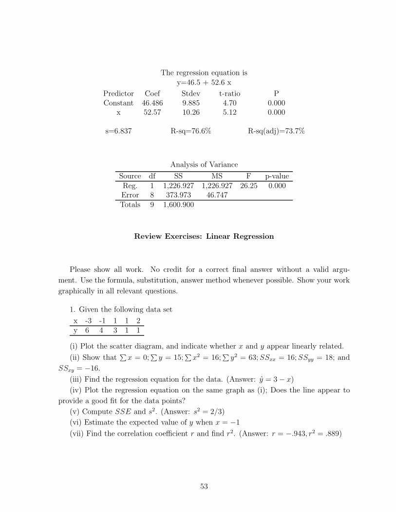
The regression equation is
y=46.5 + 52.6 x
Predictor Coef Stdev t-ratio PConstant 46.486 9.885 4.70 0.000
x 52.57 10.26 5.12 0.000
s=6.837 R-sq=76.6% R-sq(adj)=73.7%
Analysis of Variance
Source df SS MS F p-valueReg. 1 1,226.927 1,226.927 26.25 0.000Error 8 373.973 46.747Totals 9 1,600.900
Review Exercises: Linear Regression
Please show all work. No credit for a correct final answer without a valid argu-
ment. Use the formula, substitution, answer method whenever possible. Show your work
graphically in all relevant questions.
1. Given the following data set
x -3 -1 1 1 2y 6 4 3 1 1
(i) Plot the scatter diagram, and indicate whether x and y appear linearly related.
(ii) Show that∑
x = 0;∑
y = 15;∑
x2 = 16;∑
y2 = 63;SSxx = 16;SSyy = 18; and
SSxy = −16.
(iii) Find the regression equation for the data. (Answer: y = 3− x)
(iv) Plot the regression equation on the same graph as (i); Does the line appear to
provide a good fit for the data points?
(v) Compute SSE and s2. (Answer: s2 = 2/3)
(vi) Estimate the expected value of y when x = −1
(vii) Find the correlation coefficient r and find r2. (Answer: r = −.943, r2 = .889)
53
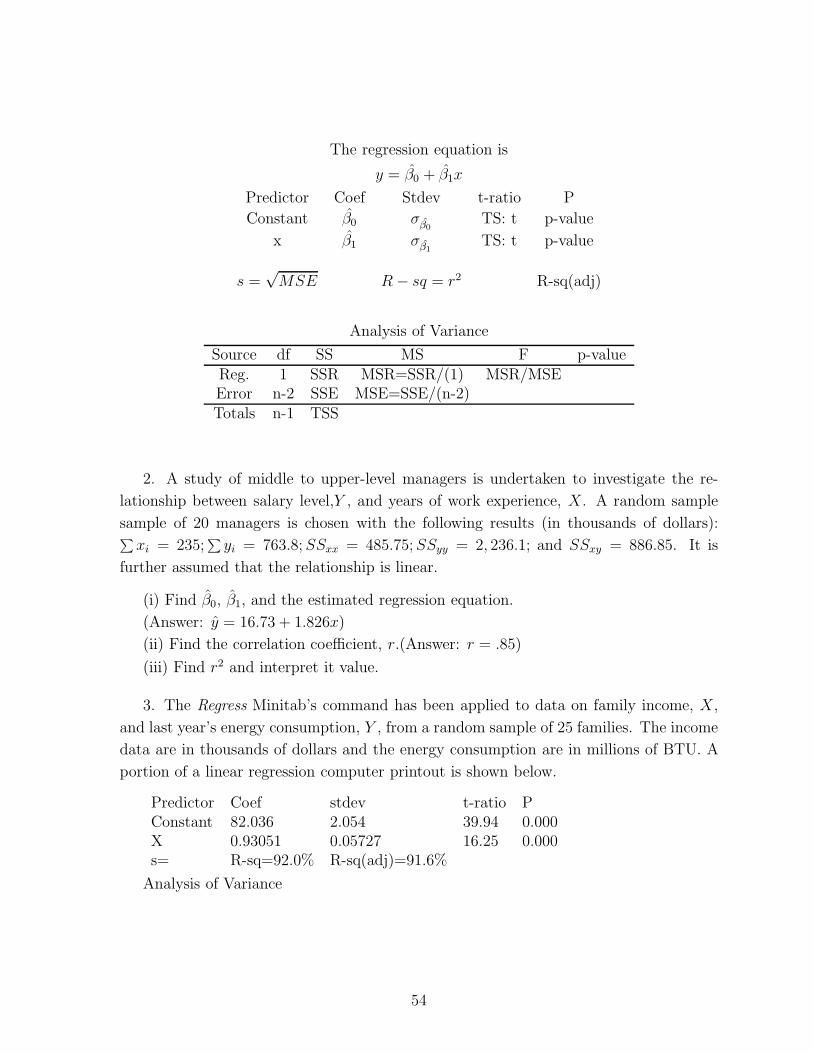
The regression equation is
y = β0 + β1x
Predictor Coef Stdev t-ratio P
Constant β0 σβ0TS: t p-value
x β1 σβ1TS: t p-value
s =√MSE R− sq = r2 R-sq(adj)
Analysis of Variance
Source df SS MS F p-valueReg. 1 SSR MSR=SSR/(1) MSR/MSEError n-2 SSE MSE=SSE/(n-2)Totals n-1 TSS
2. A study of middle to upper-level managers is undertaken to investigate the re-
lationship between salary level,Y , and years of work experience, X. A random sample
sample of 20 managers is chosen with the following results (in thousands of dollars):∑xi = 235;
∑yi = 763.8;SSxx = 485.75;SSyy = 2, 236.1; and SSxy = 886.85. It is
further assumed that the relationship is linear.
(i) Find β0, β1, and the estimated regression equation.
(Answer: y = 16.73 + 1.826x)
(ii) Find the correlation coefficient, r.(Answer: r = .85)
(iii) Find r2 and interpret it value.
3. The Regress Minitab’s command has been applied to data on family income, X,
and last year’s energy consumption, Y , from a random sample of 25 families. The income
data are in thousands of dollars and the energy consumption are in millions of BTU. A
portion of a linear regression computer printout is shown below.
Predictor Coef stdev t-ratio PConstant 82.036 2.054 39.94 0.000X 0.93051 0.05727 16.25 0.000s= R-sq=92.0% R-sq(adj)=91.6%
Analysis of Variance
54

Source DF SS MS F PRegression 7626.6 264.02 0.000Error 23Total 8291
(i) Complete all missing entries in the table.
(ii) Find β0, β1, and the estimated regression equation.
(iii) Do the data present sufficient evidence to indicate that Y and X are linearly
related? Test by using α = 0.01.
(iv) Determine a point estimate for last year’s mean energy consumption of all families
with an annual income of $40,000.
4. Answer by True of False . (Circle your choice).
T F (i) The correlation coefficient r shows the degree of association between x and y.
T F (ii) The coefficient of determination r2 shows the percentage change in y resulting
form one-unit change in x.
T F (iii) The last step in a simple regression analysis is drawing a scatter diagram.
T F (iv) r = 1 implies no linear correlation between x and y.
T F (v) We always estimate the value of a parameter and predict the value of a
random variable.
T F (vi) If β1 = 1, we always predict the same value of y regardless of the value of x.
T F (vii) It is necessary to assume that the response y of a probability model has a
normal distribution if we are to estimate the parameters β0, β1, and σ2.
55
Chapter 7
Multiple Linear Regression
Contents.
1. Introduction: Example
2. Multiple Linear Model
3. Analysis of Variance
4. Computer Printouts
1 Introduction: Example
Multiple linear regression is a statistical technique used predict (forecast) the value
of a variable from multiple known related variables.
2 A Multiple Linear Model
Model.
Y = β0 + β1X1 + β2X2 + β3X3 + ε
where
xi : independent variables (predictors)
y: dependent variable (response)
βi : unknown parameters.
ε : random error due to other factors not included in the model.
Assumptions.
1. E(ε) := µε = 0.
2. V ar(ε) := σ2ε = σ2.
3. ε has a normal distribution with mean 0 and variance σ2.
56

4. The random components of any two observed y values are independent.
3 Least Squares Prediction Equation
Estimated Regression Equation
y = β0 + β1x1 + β2x2 + β3x3
This equation is obtained by using the method of least squares
Multiple Regression Data
Obser. y x1 x2 x3
1 y1 x11 x21 x31
2 y2 x12 x22 x32
· · · · · · · · · · · · · · ·n yn x1n x2n x3n
Minitab Printout
The regression equation is
y = β0 + β1x1 + β2x2 + β3x3
Predictor Coef Stdev t-ratio P
Constant β0 σβ0TS: t p-value
x1 β1 σβ1TS: t p-value
x2 β2 σβ2TS: t p-value
x3 β3 σβ3TS: t p-value
s =√MSE R2 = r2 R2(adj)
Analysis of Variance
Source df SS MS F p-valueReg. 3 SSR MSR=SSR/(3) MSR/MSEError n− 4 SSE MSE=SSE/(n-4)Totals n− 1 TSS
57

Source df SSx1 1 SSx1x1
x2 1 SSx2x2
x3 1 SSx3x3
Unusual observations (ignore)
58

MINITAB.
Use REGRESS command to regress y stored in C1 on the 3 predictor variables stored
in C2− C4.
MTB> Regress C1 3 C2-C4;
SUBC> Predict x1 x2 x3.
The subcommand PREDICT in Minitab, followed by fixed values of x1, x2, and x3
calculates the estimated value of y (Fit), its estimated standard error (Stdev.Fit), a 95%
CI for E(y), and a 95% PI for y.
Example. A county assessor wishes to develop a model to relate the market value, y, of
single-family residences in a community to the variables:
x1 : living area in thousands of square feet;
x2 : number of floors;
x3 : number of bedrooms;
x4 : number of baths.
Observations were recorded for 29 randomly selected single-family homes from res-
idences recently sold at fair market value. The resulting prediction equation will then
be used for assessing the values of single family residences in the county to establish the
amount each homeowner owes in property taxes.
A Minitab printout is given below:
MTB> Regress C1 4 C2-C5;
SUBC> Predict 1.0 1 3 2;
SUBC> Predict 1.4 2 3 2.5.
The regression equation is
y = −16.6 + 7.84x1 − 34.4x2 − 7.99x3 + 54.9x4
Predictor Coef. Stdev t-ratio PConstant −16.58 18.88 −0.88 0.389
x1 7.839 1.234 6.35 0.000x2 −34.39 11.15 −3.09 0.005x3 −7.990 8.249 −0.97 0.342x4 54.93 13.52 4.06 0.000
s = 16.58 R2 = 88.2% R2(adj) = 86.2%
59

Analysis of Variance
Source df SS MS F p-valueReg. 4 49359 12340 44.88 0.000Error 24 6599 275Totals 28 55958
Source df SSx1 1 44444x2 1 59x3 1 321x4 1 4536
Fit Stdev.Fit 95%C.I. 95%P.I.113.32 5.80 (101.34, 125.30) (77.05, 149.59)137.75 5.48 (126.44, 149.07) (101.70, 173.81)
60
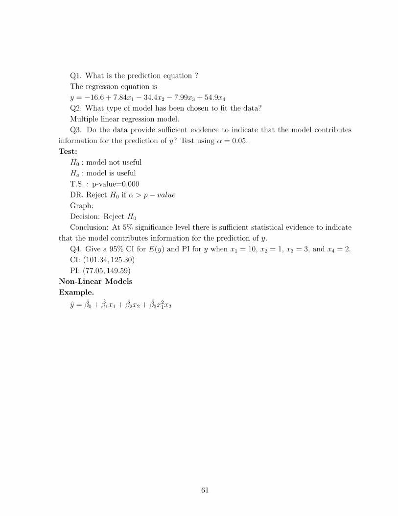
Q1. What is the prediction equation ?
The regression equation is
y = −16.6 + 7.84x1 − 34.4x2 − 7.99x3 + 54.9x4
Q2. What type of model has been chosen to fit the data?
Multiple linear regression model.
Q3. Do the data provide sufficient evidence to indicate that the model contributes
information for the prediction of y? Test using α = 0.05.
Test:
H0 : model not useful
Ha : model is useful
T.S. : p-value=0.000
DR. Reject H0 if α > p− value
Graph:
Decision: Reject H0
Conclusion: At 5% significance level there is sufficient statistical evidence to indicate
that the model contributes information for the prediction of y.
Q4. Give a 95% CI for E(y) and PI for y when x1 = 10, x2 = 1, x3 = 3, and x4 = 2.
CI: (101.34, 125.30)
PI: (77.05, 149.59)
Non-Linear Models
Example.
y = β0 + β1x1 + β2x2 + β3x21x2
61