MASTER THESIS

Power Efficiency Enhancement of Transmitters using Adaptive Envelope Tracking and Shaping Techniques for

Small Payload Space Applications

Hafiz Faisal Rasool

SUPERVISED BY

Pere Lluís Gilabert Pinal

Gabriel Montoro Lopez

Master in Aerospace Science and Technology

UNIVERISTAT POLITÈCNICA DE CATALUNYA

September 2015

Page intentionally left blank

1

Acknowledgments

In the name of God, the most Gracious, the most Merciful.

First of all, I want to express my sincerest gratitude towards my project supervisor, Mr. Pere L.

Gilabert who has guided me throughout the course of this work with his tremendous amount of

support and knowledge. He has helped me understand and resolve every issue with extreme

patience. I would also like to thank my co-supervisor Mr. Gabriel Montoro who has been really

helpful with his feedback on every step of the way during my work at Signals Theory and

Communications (TSC) Lab, UPC.

Studying at EETAC has been a magnificent opportunity for me and I want to thank all my fellows

at MAST who have made this experience even more rewarding in terms of knowledge and

growth. I would want to thank everyone at my organization, SUPARCO, who has supported me

during my studies at UPC.

My acknowledgement extends to all of my friends especially Minhaj Usmani who have stood by

me throughout my life and I am indebted to every one of them.

Ultimately, everything that I have achieved in my life is due to unconditional love and relentless

support of my parents and I want to thank everyone in my family for believing in me especially

my father who has helped me grow into the person I am and urged me to always take that one

more step.

2

Page intentionally left blank

3

Abstract

With the rise of modular system architecture for distributed satellite systems with multiple

small payloads instead of conventional larger spacecrafts, the efficient characterization of

power budget and available power constraints become even more vital. In order to establish

high data rate downlink communications in small satellite applications, use of highly

efficient, non-conventional power amplification techniques is going to be a key factor in

future communication systems. The concept of having small, less power consuming and high

data rate transmission system extends to vast number of applications like light weight

Unmanned Aerial Vehicle (UAV) and hand-held communication modules etc.

The idea is to study and develop an adaptive envelope tracking technique which should be

able to dynamically supply power to Radiofrequency power amplifier. Consequently, an

optimal control over system power consumption leads to enhanced efficiency. The amplifiers

intended for such systems exhibit nonlinear behavior when it comes to operating at maximum

output power and cause distortion in adjacent bands. Introducing a power supply modulation

block in combination with digital linearization techniques such as DPD offers considerable

improvement.

This thesis tests a dynamic power supply adaptive shaping technique for LTE signals. In

comparison to conventional fixed supply RF PAs, Envelope Tracking PA has resulted in

improved linearity at the output as well as reduced unwanted power leakage into adjacent

frequency channels. By imposing an isogain trajectory trough the shaping function, we can

optimize the available power for high data rate communications while keeping the

intermodulation distortion at acceptable levels by considering a tradeoff between efficiency

and computational load.

4

Page intentionally left blank

5

Contents

Acknowledgments ................................................................................................................................. 2

Abstract .................................................................................................................................................. 4

List of Tables ......................................................................................................................................... 8

List of Figures ........................................................................................................................................ 9

Glossary ............................................................................................................................................... 10

1 Introduction ................................................................................................................................. 12

1.1 Motivation ............................................................................................................................. 12

1.2 Objective and Methodology .................................................................................................. 14

1.3 Thesis Outline ....................................................................................................................... 15

2 High Efficiency PAs and Linearity ............................................................................................ 16

2.1 Problem Definition ................................................................................................................ 16

2.2 Power Added Efficiency ....................................................................................................... 16

2.3 Signal Characteristics ............................................................................................................ 17

2.4 PA Basics .............................................................................................................................. 18

2.4.1 Nonlinear Memoryless Model ...................................................................................... 20

2.4.2 Memory Effect on PA Models ...................................................................................... 21

2.5 Performance Characterization ............................................................................................... 21

2.6 PA Model Estimation ............................................................................................................ 23

3 Envelope Tracking and Shaping for Power Amplifiers ........................................................... 26

3.1 Fundamentals of Envelope Tracking .................................................................................... 26

3.2 ET System Architecture ........................................................................................................ 28

3.3 Efficiency Vs Linearity for ET PAs ...................................................................................... 29

3.4 Performance Enhancement of RF PA ................................................................................... 29

3.4.1 Digital Pre-Distortion .................................................................................................... 30

3.5 Envelope Shaping Function .................................................................................................. 32

3.5.1 Adaptive Iso-Gain Shaping Model................................................................................ 33

3.6 Manual Envelope Shaping and Spline Model ....................................................................... 34

3.6.1 Linear Splines ............................................................................................................... 35

3.6.2 Quadratic Splines .......................................................................................................... 37

3.6.3 Cubic Splines ................................................................................................................ 38

3.7 Manual Isogain Shaping ........................................................................................................ 41

3.7.1 Isogain Line or Targeted Gain ...................................................................................... 42

4 Experimental Setup .................................................................................................................... 44

6

4.1 Device-Under-Test Setup ...................................................................................................... 44

4.2 DUT Test Scenarios .............................................................................................................. 45

4.2.1 Dynamic Supply with No Shaping ................................................................................ 47

4.2.2 Adaptive Shaping .......................................................................................................... 48

4.2.3 Adaptive Shaping with IQ DPD .................................................................................... 50

4.3 Performance Comparison ...................................................................................................... 53

4.3.1 Manual Shaping vs Adaptive Shaping .......................................................................... 53

4.3.2 Spline Interpolated Manual Shaping Model ................................................................. 54

5 Conclusion ................................................................................................................................... 59

Bibliography ........................................................................................................................................ 61

7

List of Tables

Table 2-1: Comparison of PAPR values with PA Efficiency ............................................................... 18 Table 2-2: System Order and NMSE .................................................................................................... 24 Table 3-1: Spline Model Estimation performance for sinusoidal test function .................................... 40 Table 4-1: Test Parameters ................................................................................................................... 46 Table 4-2: Performance Comparison .................................................................................................... 53 Table 4-3: Manual vs Adaptive Shaping ............................................................................................... 54 Table 4-4: Input Envelope and Power Supply ...................................................................................... 56

8

List of Figures Figure 1-1: Distributed Satellite Systems ............................................................................................. 13 Figure 2-1: Generic Block Diagram of a Wireless Communication System ........................................ 19 Figure 2-2: PA Block ............................................................................................................................ 19 Figure 2-3: Input-Output Response curves for an Ideal and Real PA ................................................... 20 Figure 2-4: Linear Output and Intermodulation Products ..................................................................... 22 Figure 2-5: AM-AM Response of PA ................................................................................................... 23 Figure 2-6: Memoryless PA Model for 5 MHz LTE Signal ................................................................. 25 Figure 2-7: PA Model with 2 Memory Taps for 5 MHz LTE Signal ................................................... 25 Figure 3-1: Power Supply Architecture ................................................................................................ 27 Figure 3-2: Envelope and Transmitted Power ...................................................................................... 27 Figure 3-3: ET PA Block Diagram ....................................................................................................... 28 Figure 3-4: DPD Principle with Resultant Signal Spectrum ................................................................. 30 Figure 3-5: Device Efficiency and Output Power ................................................................................. 31 Figure 3-6: Efficiency and Gain Vs System Output (Optimum Efficiency Shaping) ........................... 32 Figure 3-7: ET PA with Envelope Shaping Block ................................................................................ 33 Figure 3-8: Spline Fitting ...................................................................................................................... 35 Figure 3-9: Linear Splines .................................................................................................................... 36 Figure 3-10: Linear Spline Interpolated Sine function ......................................................................... 36 Figure 3-11: Quadratic Spline Interpolated Sine function .................................................................... 38 Figure 3-12: Cubic Spline Interpolated Sine function .......................................................................... 40 Figure 3-13: Measured DC Supply and Back-off for LTE 5MHz signal .............................................. 41 Figure 3-14: Gain vs Output Power for LTE 5MHz signal .................................................................. 42 Figure 3-15: Gain vs Input Power (Targeted Gain = 35.2667dB) ........................................................ 43 Figure 3-16: Gain vs Input Power (Targeted Gain = 39.267dB) .......................................................... 43 Figure 4-1: Block Diagram of Testbed ................................................................................................. 45 Figure 4-2: Instruments Layout............................................................................................................. 45 Figure 4-3: 5 MHz Input Signal Spectra ............................................................................................... 46 Figure 4-4: AM-AM Curve for Dynamic Supply Model without shaping function ............................. 47 Figure 4-5: AM-PM Response for Dynamic Supply Model with shaping function ............................. 47 Figure 4-6: RF Output Spectrum for Dynamic Supply Model without shaping function ..................... 48 Figure 4-7: AM-AM Curve for Adaptive Shaping Model .................................................................... 49 Figure 4-8: AM-PM Response for Adaptive Shaping Model ............................................................... 49 Figure 4-9: RF Output Spectrum for Adaptive Shaping Model ............................................................ 50 Figure 4-10: Shaping Function curve for Adaptive Shaping Model ..................................................... 50 Figure 4-11: AM-AM Response for AS + IQ DPD .............................................................................. 51 Figure 4-12: AM-PM Response for AS + IQ DPD ............................................................................... 51 Figure 4-13: RF Output Spectrum for AS + IQ DPD ........................................................................... 52 Figure 4-14: Shaping Function curve for AS + IQ DPD ...................................................................... 52 Figure 4-15: Gain vs Input Power (Targeted Gain = 35.2667dB) ........................................................ 55 Figure 4-16: Gain vs Input Power (Targeted Gain = 39.267dB) .......................................................... 55 Figure 4-17: Shaping Model (35.2667dB Gain) ................................................................................... 57 Figure 4-18: Shaping Model (39.267dB Gain) ..................................................................................... 57

9

Glossary

ACPR ACPR Adjacent Channel Power Ratio ACEPR Adjacent Channel Error Power Ratio ACLR Adjacent Channel Leakage Ratio AM Amplitude Modulation DC Direct Current DE Drain Efficiency DPD Digital Predistortion EA Envelope Amplifier FPGA Field-programmable Gate Array IQ In-phase/Quadrature LTE Long-Term Evolution NMSE Normalized Mean Squared Error PA Power Amplifier PAE Power Added Efficiency PAPR Peak-to-Average Power Ratio PM Phase Modulation RF Radiofrequency WCDMA Wideband Code Division Multiple Access

10

Page intentionally left blank

11

1 Introduction

This thesis discourses the need and methodology to enhance power efficiency of modern

communication modules which range from handheld devices to small payload space

applications. Over the years, performance of radio communication standards has been

improved with the emergence next out of the box idea until the system saturates its resources

such as available power and RF spectrum. Therefore, it is vital to achieve optimal resource

utilization by exploiting the characteristics of key components like power amplifier.

In a typical RF communication system, PA is the most power hungry component, and the fact

that it also presents a non-linear behavior for different operating regions warrants thorough

study. When it comes to PAE of modern communication standards (Wi-Fi, LTE), the

conventional fixed supply PAs limit the system performance because for a rapidly varying

input signal with high ‘Peak-to-Average Power Ratio’ (PAPR) values, a lot of power is

wasted in amplifying signals with low input power. A significant drop in PAE from GSM (65

%) to LTE (30 %) highlights the challenge [1]. This objective of the thesis is to study

techniques for improving PAE by and test an algorithm on a ‘Device-Under-Test’ (DUT) to

understand how a more dynamic control over power supply to a PA offers improved resource

utilization. The idea lends its applications to power constrained nanosatellites, where the need

to use less power to transfer maximum amount of information is ever increasing.

1.1 Motivation

The importance of understanding and exploring the possibility to improve system

performance on component level is justified by the sheer volume of communication industry.

The applications of an efficient communication system range from mobile devices to

completely autonomous satellites. Telecommunications industry amasses a volume of

approximately $5 Trillion worldwide. In 2013, mobile industry contributed to 3.6 % global

GDP and this figure is expected to rise to 5.1 % in 2020. This segment of telecommunication

industry has seen the most dramatic rise in just over 10 years. In 2003, there were

approximately one billion unique subscribers and this has risen to 3.4 billion unique

subscribers worldwide in 2013 with 6.9 billion SIM connections [2]. Satellite communication

industry makes up for more than 60 % of the $195 Billion global satellite business. More than

50 % of operating satellites are primarily for communication and more than 40 % of these

satellites are used for commercial communication systems and services providing civilian

12

users with satellite broadcasting, telephony, navigation and location based services. An

increase in telecommunication industry revenues by 7 % in 2013 emphasizes that the demand

is still increasing and further research and development of means is mandated [3].

From space applications perspective, clustered or distributed satellite systems with modular

designs instead of huge single unit missions are a way forward. As a spacecraft is divided

into different small satellites flying in close proximity formations, the power resources

become fewer, whereas the demand of instantaneous handshakes and huge chunks of data

exchange between multiple systems rises. The problem can be addressed with the use of

extremely efficient PA for communication system which makes use of dynamic power supply

schemes based on the kind of information being exchanged. The system configuration is

illustrated in the fig. 1-1 [4].

Figure 1-1: Distributed Satellite Systems

With the advent of high data rate communication standards, strict linearity and bandwidth

requirements have been put in place for infrastructure and mobile applications.

PA is the most power consuming component in the transmitter chain with value of power

used by PA alone rising up to 85 % [5], whereas the PAE is relatively low (< 50 %) for non-

infrastructure applications. Traditional fixed supply PAs can be replaced with Envelope

Tracking linear RF PA with a supply modulating circuitry to increase performance. Higher

throughput gave rise to complex digital modulation schemes such as quadrature amplitude

modulation (QAM) and orthogonal frequency division multiplexing (OFDM). However, the

13

resultant signals have higher PAPR values, which have increased from 0 dB (GSM) to more

than 10 dB for LTE [1]. Strong peaks of input signal as compared to moderate average power

levels cause saturation at the output. Therefore, PAs need to operate below their maximum

output power to avoid this phenomenon but the result is decreased efficiency. Use of a

dynamic supply modulation technique ensures that PA operates in compression (high

efficiency) for a wider range of input signals. The added advantage of ET PAs over fixed

supply PA is considerably less heat dissipation improving component life time.

The statistics of high PAPR signals suggest that ET PAs spend more time operating at lower

supply voltages whereas the higher instantaneous peaks are relatively few. Therefore, ET

amplifiers are matched to be optimized for targeted high PAPR signals because generally RF

PAs are configured to operate below high efficiency region in order to avoid compression

caused by high peak values of input signal.

1.2 Objective and Methodology

The aim of this thesis is to study and comprehend the fundamentals of power amplification

for RF communication. By understanding how the previous transmission standards evolved

into newer high speed and efficient techniques, it is established that PAE is the figure of

merit that primarily defines a system’s performance. Identification of the problem leads to

study of an alternative strategy to conventional fixed supply PAs for high PAPR applications.

A system where dynamically varying power supply is modulated based on the input power of

baseband signal is implemented. Instead of using a constant supply voltage for PA, where a

sizeable amount of power was lost in heat dissipation, PAE is improved by introducing an

input envelope tracking and shaping function which controls an Envelope Amplifier or supply

modulator. Efficiency however, is not only dependent on RF PA and envelope amplifier but

the computational complexity of linearization algorithm which is used to compensate for

nonlinear distortion appearing at RF PA output. Therefore, an efficient linearization

technique also plays a vital role towards system performance. ET and shaping block is used

to perform magnitude calculation of complex digital signal, and an instantaneous power

supply voltage can be chosen. Characterization of PA behavior over a range of supply values

is performed using gain vs output power. It then becomes convenient to target either a fixed

output gain at the cost of efficiency with upside being smaller distortion in PA output. A

tradeoff can be made between linearity and efficiency by also understanding optimum

efficiency shaping in which the PA is made to operate in compression over a wide range of

14

output power values. Another aspect of the work is to study Spline interpolation that is used

for mapping required instantaneous power supply level against an envelope sample value.

Following step-wise approach is adopted:

• Study of PA performance characteristics and behavioral modelling

• Envelope Tracking and Shaping function simulation with Spline Interpolation

• System level tests of algorithm with DUT and analysis of results

1.3 Thesis Outline

The work presented in the thesis follows a modular approach starting with PA efficiency

improvement as objective, establishing envelope tracking PAs as a viable alternative it

concludes with experimental setup and simulation results using a real time test-bed.

Chapter 2 includes problem identification, an overview of basics of the PA, performance

characteristics and figures of merit. Keeping in view the objective, a tradeoff between

linearity and system efficiency is discussed for acceptable performance standards.

Chapter 3 develops the theory of Envelope Tracking amplifiers, envelope shaping function

and use of dynamic power supply for PA to enhance performance. Iso-gain characteristics

with system level block diagram and architecture of close-loop envelope tracking and shaping

functional blocks. Spline Interpolation theory and an algorithm to identify a cubic spline

model concludes the chapter.

Chapter 4 introduces hardware test-bed, experimental results with adaptive and non-adaptive

envelope shaping. Digital Pre-Distortion technique for AM-PM distortion reduction is

introduced in RF signal path to PA and results are analyzed.

Chapter 5 provides a conclusion of thesis summarizing the objective and outcome of the

project developed.

15

2 High Efficiency PAs and Linearity

Power amplifiers are the most critical block in a transmission chain with the requirement to

produce high power RF output by amplifying an input RF signal with the use of DC power

supply voltage. The amplified RF signal is then used for a reliable information transfer

between user equipment (UE) and base stations (BTSs) in mobile communication

applications. The available system resources such as power and bandwidth are limited and

strictly monitored. Infrastructure based applications such as BTS usually have more power at

their disposal but power utilization becomes extremely critical for handheld communication

modules. Since RF PAs support most of the global communication standards like GSM,

WCDMA and LTE, it is critical to understand the relation between power consumption

requirements and efficiency.

2.1 Problem Definition

Generally, in communication systems’ evolution the emphasis has been on high data rate and

maximum spectrum utilization. Emerging standards such as WCDMA, high speed packet

access (HSPA) and long term evolution (LTE) use modulated signals with a rapidly varying

envelope. A performance metric is introduced to define signal characteristics known as

PAPR. It compares peak output value to time-average output power value. High PAPR meant

that PAs transmitted peak power on relatively fewer occasions and operated at low output

powers. For fixed supply RF PAs, it means that a minor portion of DC power supply is used

for amplification of input signal and rest is dissipated in heat losses. Therefore, efficiency

drops because PAs exhibit maximum performance when operated in compression. An

alternative approach to fixed supply PA is to dynamically vary DC power supply keeping the

operation of PA in high efficiency region. An improved PAE is the objective for considering

the above mentioned modulated DC supply approach.

2.2 Power Added Efficiency

Ideally, all DC power consumed by a PA should appear at the output which is not the case for

real systems. For PAs, there are two parameters called Drain Efficiency (DE) and Power

Added Efficiency (PAE) which characterize an amplifier. DE is the ratio of output power to

the consumed DC power supply.

16

𝐷𝐷𝐷𝐷 =𝑃𝑃𝑜𝑜𝑜𝑜𝑜𝑜𝑃𝑃𝐷𝐷𝐷𝐷

× 100 % (2.1)

Pout is transmitted RF power at the output and PDC is DC power consumed for amplification.

DE defines how much of DC power is converted into output power but it does not provide a

measure of input RF power which is fed to PA for amplification. For a single stage RF PA,

the incident RF power in input signal is considerable. However DE is an important quantity

when the efficiency based on an Envelope Tracking PA and supply modulator circuitry is

considered.

PAE becomes a comprehensive figure of merit to define RF PA performance because it is

measure of power conversion efficiency, taking into account the amount of RF power in the

input signal as well.

𝑃𝑃𝑃𝑃𝐷𝐷 = 𝑃𝑃𝑜𝑜𝑜𝑜𝑜𝑜 − 𝑃𝑃𝑖𝑖𝑖𝑖

𝑃𝑃𝐷𝐷𝐷𝐷 × 100 % (2.2)

Pin is input RF signal power. Eq. 2.2 shows that a PA with higher PAE value has a longer

operation time from a power constrained application’s perspective.

2.3 Signal Characteristics

Based on the objective of finding an efficient RF power amplification scheme, the need to

understand modern signals which are used for high data rate transmission standards is

paramount. Complex, multicarrier digital modulation schemes provide high data rates and the

input signal characteristics have changed but high level system requirements are constrained

by physical system limits i.e. an RF PA usually defines performance limits of a system. There

is a demand of linearity from RF PA even at peak output powers keeping the distortion

limited, but a PA optimized for high linearity drops in efficiency except for signal peaks

which are fewer in high PAPR signals. Therefore, Linearity and efficiency tradeoff requires

understanding of shape of the signal.

Crest Factor (C) is a term which defines the spectrum characteristics of the signal. It is a ratio

between the signal peak amplitude Apeak and RMS value of signal power PRMS. Physically, it

describes how extreme the peaks are in a signal.

𝐶𝐶 = 𝑃𝑃𝑝𝑝𝑝𝑝𝑝𝑝𝑝𝑝�𝑃𝑃𝑅𝑅𝑅𝑅𝑅𝑅

(2.3)

17

PAPR is a logarithmic indicator of crest factor for RF communication which is defined as;

𝑃𝑃𝑃𝑃𝑃𝑃𝑃𝑃 = 20𝑙𝑙𝑙𝑙𝑙𝑙10(𝐶𝐶2) (2.4)

Modulation schemes with higher crest factor tend to have higher energy content in adjacent

channels causing interference. Due to systematic regulations, efficiency drops rapidly

because PA is backed-off to operate in linear region. Table 2-1 [1] lists PAPR values for

different communication standards. Over the years, as spectral efficiency or optimum

bandwidth usage increases and high data rates are achieved, PAPR value has increased

significantly. However PAE drops by a factor of 2 from GSM to LTE emphasizing the need

to find an alternative with acceptable efficiency values for high PAPR signals.

Table 2-1: Comparison of PAPR values with PA Efficiency

Transmission

Standard

Launch Year Spectral

Efficiency

bits/sec/Hz

PAPR

dB

PA Efficiency

%

GSM 2003 0.17 0 65

W-CDMA 2003 0.1 3.4 45

HSUPA 2008 1.5 6.5 35

Wi-Fi 2008 0.9 9.0 25

LTE 2010 4.0 8.0 30

2.4 PA Basics

The RF PA is an essential device which transforms DC power into RF/microwave output

power based on the input RF signal. In a communication system chain, PA sits before the

radiating devices i.e. antennae as shown in the system block diagram (Fig. 2-1). In a black-

box representation, output is generally a scaled version of input with the amplifier gain G

being the multiplying factor (Fig. 2-2). However, in a system level analysis of PA, two very

critical aspects require consideration. ‘Non-linearity’ and ‘Memory Effect’ of PA will be

discussed in the following section.

18

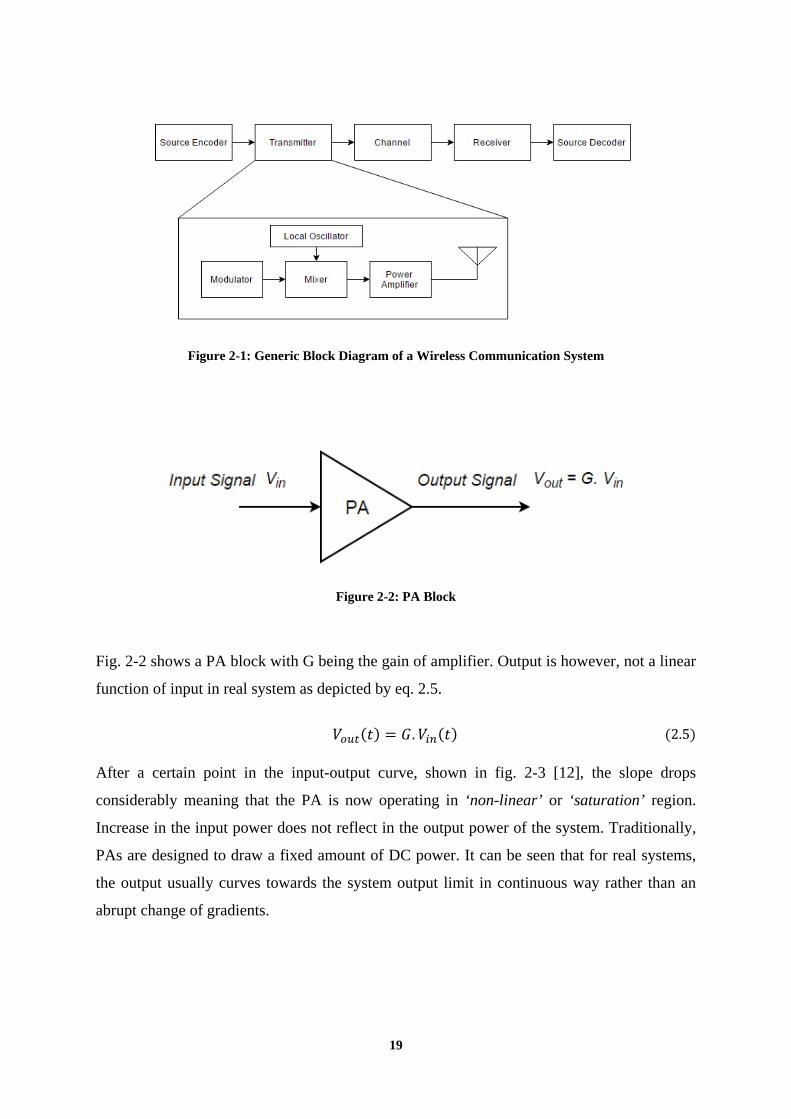
Figure 2-1: Generic Block Diagram of a Wireless Communication System

Figure 2-2: PA Block

Fig. 2-2 shows a PA block with G being the gain of amplifier. Output is however, not a linear

function of input in real system as depicted by eq. 2.5.

𝑉𝑉𝑜𝑜𝑜𝑜𝑜𝑜(𝑡𝑡) = 𝐺𝐺.𝑉𝑉𝑖𝑖𝑖𝑖(𝑡𝑡) (2.5)

After a certain point in the input-output curve, shown in fig. 2-3 [12], the slope drops

considerably meaning that the PA is now operating in ‘non-linear’ or ‘saturation’ region.

Increase in the input power does not reflect in the output power of the system. Traditionally,

PAs are designed to draw a fixed amount of DC power. It can be seen that for real systems,

the output usually curves towards the system output limit in continuous way rather than an

abrupt change of gradients.

19

Figure 2-3: Input-Output Response curves for an Ideal and Real PA

The input-output curve is then divided into linear and compression region. It is important to

note that in linear systems, the principle of superposition applies. A linear system with the

model shown in equation

𝑦𝑦 = 𝐹𝐹{𝑥𝑥} (2.6)

will produce an output 𝑎𝑎1𝐹𝐹{𝑥𝑥1} + 𝑎𝑎2𝐹𝐹{𝑥𝑥2}, for an input 𝑎𝑎1𝑥𝑥1 + 𝑎𝑎2𝑥𝑥2 with a scalar multiple

a, where x and y being the input and output of the system respectively. The said superposition

principle does not hold true for non-linear systems and there are additional terms in frequency

spectrum which are called intermodulation products or harmonics. Having established that an

RF PA behaves as a non-linear system, it is now important to characterize PA behavioral

model.

2.4.1 Nonlinear Memoryless Model

For narrow band signals where the envelope of input signal varies slowly, the output of PA is

a function of instantaneous input value. For a limited range of input signal amplitudes, the

memoryless nonlinear behavior of PA can be modeled using a complex power series [9].

𝑉𝑉𝑜𝑜𝑜𝑜𝑜𝑜 (𝑡𝑡) = �𝑎𝑎𝑝𝑝 .𝑉𝑉𝑖𝑖𝑖𝑖𝑝𝑝 (𝑡𝑡)∞

𝑝𝑝=0

(2.7)

Where ak is the gain of the system and it depends upon the order of the model. For the first

order system, the response is linear. With the expansion of power series, the even terms (vin2 ,

vin4 , vin6 …) produce harmonics in spectrum and the odd terms (vin3 , vin5 , vin7 , …) result in

20

intermodulation products. The Harmonic Distortion (HD) can be filtered out, while

Intermodulation Distortion (IMD) causes a bigger concern due to that fact that it is too close

to the actual signal band.

2.4.2 Memory Effect on PA Models

Memory effect in behavioral model describes the extent to which the current response of the

system is influenced by past inputs to the system. It is a very critical phenomenon in PA. If

the impact of memory is considered on the system model, then it cannot be represented by a

simple power series expansion because the scaling factors or ‘coefficients’ vary for each

memory tap [10, 11].

𝑦𝑦[𝑛𝑛] = �𝑎𝑎𝑝𝑝. 𝑥𝑥[𝑛𝑛]. |𝑥𝑥[𝑛𝑛]|𝑝𝑝 𝑃𝑃−1

𝑝𝑝=0

(2.8)

The equation 2.8 governs the system model for a complex memoryless behavior where ap is

the set of coefficients and P is number of coefficients of polynomial or system order. In case

of memory the model takes form of the equation 2.9.

𝑦𝑦[𝑛𝑛] = � �𝑎𝑎𝑝𝑝𝑖𝑖 . 𝑥𝑥[𝑛𝑛 − 𝑖𝑖]. |𝑥𝑥[𝑛𝑛 − 𝑖𝑖]|𝑝𝑝𝑃𝑃−1

𝑝𝑝=0

𝑅𝑅−1

𝑖𝑖=0

(2.9)

M is the number of memory taps or past terms used to calculate instantaneous output of PA

and P is number of coefficients of interpolating polynomial. The delayed values of input

signal are also considered in case of memory polynomial.

2.5 Performance Characterization

The accuracy and capability of PA model to mimic the real-time system can be measured

using following Figures of Merit. In discrete domain, the input and output of the model is

assessed sample by sample and the performance is expressed in dB for both Normalized

Mean Square Error (NMSE) and Adjacent Channel Error Power Ratio (ACEPR).

𝑁𝑁𝑁𝑁𝑁𝑁𝐷𝐷 = 10 log�∑ |𝑦𝑦𝑟𝑟𝑝𝑝𝑝𝑝𝑟𝑟[𝑛𝑛] − 𝑦𝑦𝑚𝑚𝑜𝑜𝑚𝑚𝑝𝑝𝑟𝑟[𝑛𝑛]|2𝐿𝐿𝑖𝑖=1

∑ |𝑦𝑦𝑟𝑟𝑝𝑝𝑝𝑝𝑟𝑟[𝑛𝑛]|2𝐿𝐿𝑖𝑖=1

� (2.10)

and

21

ACEPR = 10 log�∫ |Yreal(f) − Ymodel(f)|2dfadj

∫ |Yreal(f)|2chan df� (2.11)

where yreal and ymodel are the outputs of real system and the PA model respectively and Y (f) is

the Fourier transform of output signal and power in allocated band and adjacent band is

measure using the integrals.

Another important figure of merit that defines quality of the output RF spectrum which in

turn translates into compliance with linearity constraints is Adjacent Channel Leakage Ratio

(ACLR) or Adjacent Channel Power Ratio (ACPR). It is the ratio of power transmitted in the

allocated bandwidth to the power which seeps into sidebands due to nonlinear distortion

caused by PAs which are forced operated in high efficiency region.

𝑃𝑃𝐶𝐶𝐴𝐴𝑃𝑃 = 10 log�∫ |𝑌𝑌(𝑓𝑓)2|𝑑𝑑𝑓𝑓𝑓𝑓𝑎𝑎𝑎𝑎𝑎𝑎

∫ |𝑌𝑌(𝑓𝑓)2|𝑓𝑓𝑐𝑐ℎ𝑎𝑎𝑎𝑎𝑑𝑑𝑓𝑓� (2.12)

Where Y (f) is Fourier transform of output and 𝑓𝑓𝑝𝑝𝑚𝑚𝑎𝑎and 𝑓𝑓𝑐𝑐ℎ𝑝𝑝𝑖𝑖 are bandwidth of adjacent

channels and complete channel respectively. Fig. 2-4 [11] graphically depicts useful power

leakage into sidebands at the output and intermodulation products.

Figure 2-4: Linear Output and Intermodulation Products

22

2.6 PA Model Estimation

Following section provides a comparison between a memoryless PA model and one where

delayed inputs also impact the output of system i.e. ‘With-Memory’. Initially a memoryless

system is estimated from input and output relation of a real PA and modeled output is

compared with real output to quantify the accuracy with which the ‘black box’ has been

modeled. Subsequently, memory is also included in the estimation and results are compared.

Initial step towards PA model estimation is to get a characteristic response of PA for a

predefined input test signal. Fig. 2-5 shows a simulated response of PA for a 5 MHz LTE test

signal. Input signal bandwidth is 5 MHz and number of samples is 9216.

Figure 2-5: AM-AM Response of PA

A memoryless and with-memory PA model will be identified based on polynomials from eq.

2.4 and 2.5 in the following section. Fig. 2-6 and 2-7 show memoryless response and a PA

model with 2 memory taps for different system order values respectively. For memoryless

model identification, increasing the order of interpolating polynomial improves estimation to

an extent, after which increasing the system order only adds to computational complexity

with not so great effect on model quality. As we move to memory polynomial based

identification of PA model with 2 memory taps, each instantaneous output is the outcome of

instantaneous input and 2 previous input values. Including memory effect provides an

equivalent model quality to higher order memoryless model with the use of a lower order

polynomial.

23

Table 2-2 lists the results obtained by model estimation. Increasing polynomial order

definitely produces estimation but higher order polynomial interpolation adds to

computational cost which is a critical parameter for power constrained handheld devices.

However, pre-calculated polynomial based model can be stored into a Lookup Table (LUT)

which produces a fixed output value for a certain input. However, Lookup table size is

defined prior to input being given to PA model. With some compromise on accuracy, the

computational complexity can be reduced with a complex gain LUT. Multiple LUTs can be

implemented using FPGA if memory terms are included in PA model estimation.

Table 2-2: System Order and NMSE

Polynomial Order Memoryless PA Model

PA Model with Memory

(No. of Memory Taps = 2)

No. of

Coefficients

NMSE (dB) No. of

Coefficients

NMSE (dB)

1 (Linear) 1 -15.2191 3 -15.3867

3 3 -34.1801 9 -34.9425

5 5 -37.5177 15 -38.3528

7 7 -39.5810 21 -41.2567

24

Figure 2-6: Memoryless PA Model for 5 MHz LTE Signal

Figure 2-7: PA Model with 2 Memory Taps for 5 MHz LTE Signal

25

3 Envelope Tracking and Shaping for Power Amplifiers

The Envelope Tracking PA yields high efficiency when signals with high PAPR are

amplified. Communication standards with spectrum efficient digital modulation schemes

impose strict constraints on linearity requirements for handheld and infrastructure

applications of wireless communication. An ET PA achieves considerable efficiency by

modulating DC power supply instantaneously tracking a shaped envelope of input RF signal.

In this chapter, basics of ET are discussed with an aim to link improved system efficiency

with a dynamic supply PA technique.

3.1 Fundamentals of Envelope Tracking

The idea is to improve power efficiency of PAs with high PAPR signals. The need to achieve

higher data throughput with spectrum constraints can be met with the use of complex,

multicarrier modulation schemes. In a traditional fixed supply amplifier, energy is wasted

when the system operates below peak output power. If the envelope of information being

amplifier is constant, it is possible to adjust the supply to PA in order to optimize power

utilization. The similar approach enables GSM communication to achieve efficiency as high

as 65 % with the use of constant envelope signals.

However, as in LTE and other modern communication standards the signals are consistently

varying and optimal solution is to dynamically modify the power supply to PA to track the

requirements of signal envelope. This is achieved by performing magnitude calculation of

input signal. ‘Average Power Tracking’ scheme follows a relatively slow-varying change in

the output signal whereas ET updates the power supply requirement at a much faster I/Q sub-

sample rate. Generalized architecture of the fixed supply, DC tracking and an ET power

system is illustrated in fig. 3-1 [1].

26

Figure 3-1: Power Supply Architecture

Figure 3-2: Envelope and Transmitted Power

It can be noted that envelope detection of input signal is performed in the feed-forward path

and a supply modulator block varies the power to PA dynamically to enhance efficiency.

27

Signal’s envelope for each type of supply scheme is shown in fig. 3-2 for demonstrating how

the system resources are used efficiently by the tracking the RF envelope and modify the

supply to PA.

As detailed in the previous chapter, a PA operates at its maximum efficiency in compression

region. An obvious advantage of using ET PAs is that it can be made to operate in

compression for a wider range of outputs by maintaining a lower and constantly changing

power supply.

3.2 ET System Architecture

An ET PA system uses a linear or switched amplifier and a modulation circuit for supply

voltage i.e. Envelope Amplifier (EA). In this technique, the supply voltage is dynamically

varied according to magnitude calculations of input signal.

The digital data path for I/Q components which are fed to PA after mixing and filtering is

similar for both fixed supply and ET PA. However in ET PA, another feed-forward path is

included which tracks sub-sample level envelope. An envelope shaping function (shown in

Fig. 3-3) is used to correctly identify which power supply level is suitable for incoming input

signal level.

Figure 3-3: ET PA Block Diagram

From the block diagram, it can be noted that RF input signal denoted u[n] is fed to signal and

envelope path simultaneously. In the envelope path, magnitude calculation is performed to

identify the level of envelope denoted as E[n]. The output of envelope shaping block Es[n]

modulates DC power supply to RF PA. Dynamically varying power supply is beneficial but

28

the cost the non-linear distortion at the output. An alternative approach is to use mapping

function to linearize AM-AM distortion by fixing “targeted gain” value but using an Iso-gain

Shaping deteriorates efficiency. Additional non-linear compensation in data path is added to

reduce AM-PM distortion.

3.3 Efficiency Vs Linearity for ET PAs

The concept of ET PA seems simple enough to make it an attractive alternative to fixed

supply PAs for high PAPR transmission schemes, but limitations such as efficiency of PA,

linearity constraints specific to each standard and output power handling capacity are weak

points of schemes which employ envelope information for power supply variation.

Efficiency being the most critical figure of merit requires considerably high efficiency from

power supply modulator or EA along with an RF PA which has high peak power efficiency.

Whereas, low noise and linearity requirements for ET technique mean that not only RF PA

distortion should be controlled but also the distortion from supply modulating amplifier

should be kept on a minimum. Consequently, a tradeoff between PA efficiency and

compliance with linearity restriction is not only dependent on amplifier design but also on

supply modulator design and baseband processing.

Another important challenge in small terminal PA design and operation is handling of

bandwidth and the ability of PA to operate over various frequency bands. W-CDMA devices

may have to support to support operation across five bands because of world-wide coverage

and there lies the need for three separate sets of PA assembly [1]. This trend is going to

demand the operation across wider bands from future devices. There are various techniques

to improve efficiency when an RF PA is deployed with a supply modulator.

3.4 Performance Enhancement of RF PA

Generally, operating a PA in compression maximizes its efficiency and this is evident from

the performance of constant envelope modulation schemes e.g. GMSK used in GSM which

do not include Amplitude Modulation (AM) component. But for a modulation scheme that

includes an AM component, the output of the system will show AM-AM distortion or

‘clipping’ if the input signal has higher instantaneous PAPR and drives PA to operate in

compression. For such schemes, the PA is made to operate below the maximum output levels

so that instantaneous input envelope level itself does not cause output distortion.

29

One of the performance limiting factors for ET PAs is spectral regrowth. As discussed in

previous sections that in compression PA output AM-AM and AM-PM response is distorted

due to non-linearity. Therefore, frequency spectrum shows a stepped down degradation

energy content of the signal in adjacent channels. Each step represents the amount of useful

power being leaked to sidebands. This phenomenon is known as spectral regrowth. In order

to compensate for the said distortion, a powerful linearization technique is needed.

3.4.1 Digital Pre-Distortion

Pre-Distortion is a technique that significantly reduces AM-AM distortion by applying an

‘inverse’ distortion to signal. Once the signal is compressed by PA, the inverse distortion is

cancelled out by PA’s AM-AM distortion property and a fairly correct signal is produced at

the output of RF chain. The amount of distortion needed to rectify PA’s nonlinear impact is

estimated using a feedback path. Fig 3-4 [7] depicts the general idea of DPD process.

Figure 3-4: DPD Principle with Resultant Signal Spectrum

PA response is prior to applying an input to the system using test signal. An inverse of PA

characterization is applied to input signal and the result presents a fairly linear signal at PA

output. Frequency spectrum in Fig. 3-4 [7] shows improvement in terms of power leakage

into sidebands. This enables the possibility to use a PA at maximum output level, enhancing

the efficiency of a standard amplifier assembly. Since it a computationally complex and a

30

significant amount of signal processing is applied to baseband signal before it is input the PA,

this technique is not too feasible to be used for power-constrained, non-infrastructure small

communication modules.

DC-Tracking or Average Power Tracking is another solution which benefits from the fact

that base stations and small terminals do not always transmit at their maximum power.

Protocols “hand-shake” for the requires output power levels for a given time and power

supply to PA or Drain Supply can be adjusted to lower values which in turn improves power

efficiency to some extent.

This leads to ET PA which keeps tracks of instantaneous level of input signal, and adjusts the

power supply to match RF signal at the input of PA. Fig. 3-5 [1] shows device efficiency

versus output power for over a range of supply voltages.

Figure 3-5: Device Efficiency and Output Power

It can be seen that in case of a fixed supply PA, efficiency drops significantly when the

system is operated below maximum output power. However, dynamic supply with envelope

shaping function offers relatively constant efficiency even at lower values of output power.

31

3.5 Envelope Shaping Function

The shaping function is responsible for performance improvement of system. A DAC and

filter converts the output of shaping block into a nominal envelope waveform which is fed to

supply modulator or EA. It is however, very critical to understand the concept of path

synchronization. ‘Signal Path’ and ‘Envelope Path’ must be aligned in timing and magnitude

so that correct sample of information is amplified with correct level of supply. Following

objectives can be achieved using shaping by means of changing power supply requirement;

• Optimum Efficiency Shaping

• Iso-Gain Shaping

Optimum Efficiency Shaping function results in relatively constant system efficiency across a

range of output power. PA is operated at maximum efficiency for different supply voltages.

This technique however, introduces AM-AM distortion in the output. Gain characteristics and

Optimum efficiency curves are shown in fig. 3-6 [9].

Figure 3-6: Efficiency and Gain Vs System Output (Optimum Efficiency Shaping)

Iso-Gain Shaping optimizes the system to achieve a lower AM-AM distortion by fixing a

value for targeted output gain although the system operates in compression. In other words,

linearity is achieved while sacrificing efficiency. Iso-gain shaping provides greater degree of

compression for highest power levels resulting in absolute energy savings.

32

3.5.1 Adaptive Iso-Gain Shaping Model

The advantage to use an adaptive iso-gain shaping function it is to avoid generating prior

input-output characterization of PA using different supply voltages. Fig. 3-7 shows block

diagram of an ET PA which uses an adaptive envelope tracking and shaping function as well

as Digital Pre-Distorter (non-linear modulation) to compensate for AM-PM to some extent.

A mathematical model is developed in this section which represents the behavioral model of

an adaptive shaping block.

Figure 3-7: ET PA with Envelope Shaping Block

Working in discrete domain, the complex baseband is designated as x[n]. The first step is to

perform magnitude calculation for envelope;

𝐷𝐷[𝑛𝑛] = |𝑥𝑥[𝑛𝑛]| = | 𝑥𝑥𝐼𝐼[𝑛𝑛]2 + 𝑥𝑥𝑄𝑄[𝑛𝑛]2| = �𝑥𝑥𝐼𝐼[𝑛𝑛]2 + 𝑥𝑥𝑄𝑄[𝑛𝑛]2 (3.1)

The output of model Es [n] considering memory terms can be written as;

𝐷𝐷𝑠𝑠[𝑛𝑛] = ��𝑤𝑤𝑝𝑝,𝑖𝑖 . (𝐷𝐷[𝑛𝑛 − 𝜏𝜏𝑖𝑖])𝑝𝑝𝑃𝑃−1

𝑝𝑝=0

𝑁𝑁−1

𝑖𝑖=0

(3.2)

𝜏𝜏𝑖𝑖 is the most significant delay of the envelope that can be used to incorporate memory. The

output of the shaping model Es [n] can be written as the difference of signal envelope and a

non-linear distortion estimated using system coefficients.

33

𝐷𝐷𝑠𝑠[𝑛𝑛] = 𝐷𝐷[𝑛𝑛] − 𝜀𝜀[𝑛𝑛] (3.3)

and

𝜀𝜀[𝑛𝑛] = 𝐄𝐄𝐧𝐧.𝐰𝐰𝐧𝐧 (3.4)

𝐰𝐰𝐧𝐧 is a vector of coefficients of order ‘O’ where O = P×N. P is the system order or the no. of

polynomial coefficients and N is the no. of memory taps. Data matrix for calculation of

system coefficients consists of vectors of basis waveform and represented as Φ = (φ1, φ2, ... ,

φL)T, where L is the no. of data samples. Any vector of the data matrix can be written as φn =

(E[n],E[n]2, … , (E[n])p , … , E[n-τN-1], … , (E[n-τN-1])p

In order to make the algorithm adaptive, close loop identification approach is considered here

which updates the system coefficients based on LS algorithm.

𝐰𝐰𝐧𝐧+𝟏𝟏 = 𝐰𝐰𝐧𝐧 + 𝛍𝛍 (𝚽𝚽𝐇𝐇 𝚽𝚽)−𝟏𝟏𝚽𝚽𝐇𝐇𝐞𝐞 (3.5)

e is an error vector of length L and μ is the weighting factor.

𝐞𝐞 = �𝐲𝐲𝐆𝐆𝟎𝟎� − 𝐄𝐄 (3.6)

G0 is the linear gain of PA in order to target a particular isogain shaping whereas y and E are

PA output and signal envelope vectors, respectively.

In order to reduce the computational complexity, the isogain shaping polynomial

interpolation and estimation can be replaced by Look-Up table. Equation 3.7 presents LUT

model with GLUT being the complex gain for each memory tap.

𝐷𝐷𝑠𝑠[𝑛𝑛] = �𝐷𝐷[𝑛𝑛 − 𝜏𝜏𝑖𝑖].𝐺𝐺𝐿𝐿𝐿𝐿𝐿𝐿𝑖𝑖(𝐷𝐷[𝑛𝑛 − 𝜏𝜏𝑖𝑖])𝑁𝑁−1

𝑖𝑖=0

(3.7)

3.6 Manual Envelope Shaping and Spline Model

Shaping function uses polynomial interpolation for estimating the response of PA. However,

in data estimation and statistical analysis, spline Interpolation technique is preferred over

polynomial interpolation because the estimation error can be reduced even when the system

order is relatively lower. This reduction in model estimation error gives rise to improved

efficiency. Spline interpolation provides stability between N+1 data points by avoiding wild

oscillations while forcing the first and second derivatives to be continuous.

34

Originally, the word ‘spline’ was used for elastic rulers that were bent in order to pass

through various points called ‘knots’. The first and last or boundary points in a data set are

called ‘exterior knots’ whereas all other points are called ‘interior knots’. This technique was

used to make technical drawings in shipbuilding. An example of a typical spline is shown in

fig. 3-8. It can be noted that the gradient of function is continuous and presents stability while

fitting is performed between data points.

Figure 3-8: Spline Fitting

The importance of stability and continuous higher order derivatives is very significant in

physical phenomenon like displacement, velocity and acceleration of moving objects and

trajectory estimation functions because it minimizes potential energy of function relative to

interpolation constraints. Spline interpolation scheme’s stability increases with the increase in

the order of the function itself. Linear or Piece-wise continuous spline is the first order spline

function, whereas quadratic and cubic spline functions are higher dimensions of spline

interpolation with cubic splines being the most preferred since these offer a continuous first

and second derivate.

3.6.1 Linear Splines

Linear or 1st order spline interpolation simply joins two consecutive data points using a

straight-line (linear equation). It does not include any information about the impact the rest of

data points can have on the fitting.

A set of n+1 data points ((𝑥𝑥0,𝑦𝑦0), (𝑥𝑥1,𝑦𝑦1), (𝑥𝑥2,𝑦𝑦2), … , (𝑥𝑥𝑖𝑖,𝑦𝑦𝑖𝑖)) can be fit on linear

splines with following function. 𝑦𝑦𝑖𝑖 = 𝑓𝑓(𝑥𝑥𝑖𝑖).

35

Figure 3-9: Linear Splines

For each interval (xi ≤ x ≤ xi+1), an independent linear equation is calculated which is only

impacted by boundary knots.

𝑓𝑓(𝑥𝑥) = 𝑓𝑓(𝑥𝑥𝑖𝑖) +𝑓𝑓(𝑥𝑥𝑖𝑖+1) − 𝑓𝑓(𝑥𝑥𝑖𝑖)

𝑥𝑥𝑖𝑖+1 − 𝑥𝑥𝑖𝑖 (𝑥𝑥 − 𝑥𝑥𝑖𝑖) 𝑥𝑥𝑖𝑖 ≤ 𝑥𝑥 ≤ 𝑥𝑥𝑖𝑖+1 (3.8)

It can be noted that f(xi+1)−f(xi)xi+1− xi

is local slope for every interval. In order to understand the

concept of spline interpolation 𝑦𝑦 = sin(𝑥𝑥) is taken as an example function. Fig.3-10 shows

the linear spline model output in comparison with actual values of sine function.

Figure 3-10: Linear Spline Interpolated Sine function

36

3.6.2 Quadratic Splines

In quadratic splines, each set of points is connected using a quadratic equation. This model

provides estimation with less steeper change of direction at the interior knots. A given set of

data points ((𝑥𝑥0,𝑦𝑦0), (𝑥𝑥1,𝑦𝑦1), (𝑥𝑥2, 𝑦𝑦2), … , (𝑥𝑥𝑖𝑖,𝑦𝑦𝑖𝑖)) fits through interior knots using

following algorithm;

𝑓𝑓(𝑥𝑥) = 𝑎𝑎1𝑥𝑥2 + 𝑏𝑏1𝑥𝑥 + 𝑐𝑐1, 𝑥𝑥0 ≤ 𝑥𝑥 ≤ 𝑥𝑥1

= 𝑎𝑎2𝑥𝑥2 + 𝑏𝑏2𝑥𝑥 + 𝑐𝑐2, 𝑥𝑥1 ≤ 𝑥𝑥 ≤ 𝑥𝑥2

.

.

.

= 𝑎𝑎𝑖𝑖𝑥𝑥2 + 𝑏𝑏𝑖𝑖𝑥𝑥 + 𝑐𝑐𝑖𝑖, 𝑥𝑥𝑖𝑖−1 ≤ 𝑥𝑥 ≤ 𝑥𝑥𝑖𝑖

In order to solve this system simultaneously, 3n equations are required to calculate 3n

coefficients. Following conditions characterize quadratic splines;

Each quadratic spline passes through 02 consecutive data points.

𝑎𝑎𝑖𝑖𝑥𝑥𝑖𝑖−12 + 𝑏𝑏𝑖𝑖𝑥𝑥𝑖𝑖−1 + 𝑐𝑐𝑖𝑖 = 𝑓𝑓(𝑥𝑥𝑖𝑖−1) (3.9)

𝑎𝑎𝑖𝑖𝑥𝑥𝑖𝑖2 + 𝑏𝑏𝑖𝑖𝑥𝑥𝑖𝑖 + 𝑐𝑐𝑖𝑖 = 𝑓𝑓(𝑥𝑥𝑖𝑖) (3.10)

𝑖𝑖 = 0,1,2, … ,𝑛𝑛. Since there are n splines passing through n-1 interior knots. This condition

yields 2n equations.

The first derivative of consecutive splines is continuous at the interior knots.

For instance, the first derivative of first spline is: 2𝑎𝑎1𝑥𝑥 + 𝑏𝑏1

First derivative of second spline is: 2𝑎𝑎2𝑥𝑥 + 𝑏𝑏2

Making derivatives equal at interior knot (𝑥𝑥 = 𝑥𝑥1) gives: 2𝑎𝑎1𝑥𝑥1 + 𝑏𝑏1 − 2𝑎𝑎2𝑥𝑥1 − 𝑏𝑏2 = 0.

Generalizing the expression for all interior knots;

2𝑎𝑎𝑖𝑖𝑥𝑥𝑖𝑖 + 𝑏𝑏𝑖𝑖 − 2𝑎𝑎𝑖𝑖+1𝑥𝑥𝑖𝑖 − 𝑏𝑏𝑖𝑖+1 = 0 (3.11)

37

The above condition provides n-1 equations. 1 remaining equation is obtained by assuming

that the first spline is linear. Solving the system of equations in matrix form, results in a

vector of coefficients which are then used to estimates data between known points. It is

extremely important to note that for each interval, a separate set of coefficients for quadratic

equation is used for a precise model.

Figure 3-11: Quadratic Spline Interpolated Sine function

As shown in fig. 3-11, the interpolated function is always continuous at the interior knots i.e.

there are no sharp changes in the direction which is a prominent characteristic of spline

interpolation. However the data fitting is not as accurate as required to justify the selection of

model. Therefore, cubic splines are preferred due to the fact that they provide more stability

and accuracy.

3.6.3 Cubic Splines

Cubic spline interpolation uses a continuous first and second derivative at the interior knots.

This along with the use of boundary conditions provides more stability and a smooth

estimation of model. Therefore, cubic spline interpolation can replace polynomial

interpolation for shaping function block used in envelope path. General form of a cubic spline

interpolation model is;

𝑓𝑓𝑖𝑖(𝑥𝑥) = 𝑎𝑎𝑖𝑖𝑥𝑥3 + 𝑏𝑏𝑖𝑖𝑥𝑥2 + 𝑐𝑐𝑖𝑖𝑥𝑥 + 𝑑𝑑𝑖𝑖 𝑖𝑖 = 1,2, … ,𝑛𝑛 𝑎𝑎𝑛𝑛𝑑𝑑 𝑥𝑥𝑖𝑖−1 ≤ 𝑥𝑥 ≤ 𝑥𝑥𝑖𝑖 (3.12)

38

In order to solve s system of n cubic splines, 4n equations are needed to determine 4n

coefficients. For a given set of data points ((𝑥𝑥0, 𝑦𝑦0), (𝑥𝑥1, 𝑦𝑦1), (𝑥𝑥2,𝑦𝑦2), … , (𝑥𝑥𝑖𝑖,𝑦𝑦𝑖𝑖)),

following set of conditions governs cubic spline algorithm;

Each cubic spline passes through on end of the particular interval.

𝑎𝑎𝑖𝑖𝑥𝑥𝑖𝑖−13 + 𝑏𝑏𝑖𝑖𝑥𝑥𝑖𝑖−12 + 𝑐𝑐𝑖𝑖𝑥𝑥𝑖𝑖−1 + 𝑑𝑑𝑖𝑖−1 = 𝑓𝑓(𝑥𝑥𝑖𝑖−1) (3.13)

𝑎𝑎𝑖𝑖𝑥𝑥𝑖𝑖3 + 𝑏𝑏𝑖𝑖𝑥𝑥𝑖𝑖2 + 𝑐𝑐𝑖𝑖𝑥𝑥𝑖𝑖 + 𝑑𝑑𝑖𝑖 = 𝑓𝑓(𝑥𝑥𝑖𝑖) (3.14)

The above condition provides 2n equations for system.

Consecutive splines have continuous first derivative at interior knots.

n-1 equations are obtained from mathematical interpretation of the condition above similar to

quadratic splines.

3𝑎𝑎𝑖𝑖−1𝑥𝑥𝑖𝑖−12 + 2𝑏𝑏𝑖𝑖−1𝑥𝑥𝑖𝑖−1 + 𝑐𝑐𝑖𝑖−1 − 3𝑎𝑎𝑖𝑖𝑥𝑥𝑖𝑖−12 − 2𝑏𝑏𝑖𝑖𝑥𝑥𝑖𝑖−1 − 𝑐𝑐𝑖𝑖 = 0 (3.15)

Consecutive splines have continuous second derivative at interior knots.

The above condition provides another set of n-1 equations.

6𝑎𝑎𝑖𝑖−1𝑥𝑥𝑖𝑖−1 + 2𝑏𝑏𝑖𝑖−1 − 6𝑎𝑎𝑖𝑖𝑥𝑥𝑖𝑖−1 − 2𝑏𝑏𝑖𝑖 = 0 (3.16)

Second derivative of first and last spline at starting and ending exterior knot, respective is

equal to zero (Natural Boundary Condition).

Natural boundary conditions provide 2 equations as follows;

6𝑎𝑎1𝑥𝑥0 + 2 𝑏𝑏1 = 0 (3.17)

6𝑎𝑎𝑖𝑖𝑥𝑥𝑖𝑖 + 2 𝑏𝑏𝑖𝑖 = 0 (3.18)

In matrix notation, the coefficient vector x will have 4n elements. Solving a system of

matrices will result in a cubic spline based model.

𝐀𝐀𝐀𝐀 = 𝐛𝐛 (3.19)

39

The solution for coefficients resembles the polynomial model described in previous section.

Using equations 3.13 to 3.18, a data matrix A is constructed using input signal values. PA

output response replaces vector b and matrix multiplication yields x vector. 4n elements in x

state that each cubic spline has independent set of 4 coefficients which are used whenever an

input sample value falls in the interval interpolated by the particular spline equation.

Figure 3-12: Cubic Spline Interpolated Sine function

Table 3-1: Spline Model Estimation performance for sinusoidal test function

Order of Spline NMSE [dB] Linear -21.0261

Quadratic -10.6409 Cubic -24.9321

Table 3-1 lists NMSE values for three different types of spline interpolation (presented in

section 3.6.) with a sinusoidal test function 𝑦𝑦 = sin(𝑥𝑥) to comprehensively visualize the

stability property of spline interpolation. Because the number of interpolation points (11) is

sufficient for the size of test vector (200 equi-spaced points), there is not a significant

difference in quality of linear and cubic splines. However, the stability characteristics (shown

in fig. 3-12) and close to real estimation by cubic spline makes it an alternative to replace

polynomial interpolation in envelope shaping block for model estimation. Cubic spline

40

interpolation model will be presented as an alternative to polynomial model for manual

shaping block.

3.7 Manual Isogain Shaping

Following section discusses the prospect of using manual envelope shaping (by hand) using

cubic spline interpolation model established in 3.6.3 instead of using polynomial

interpolation. It has been discussed how using spline interpolation improves stability of

estimated data. The input-output response or the transfer function of PA is characterized

using a 5 MHz LTE signal. PA is supplied with a set of drain voltage based on input signal

envelope and response in terms of input power, output power and gain has been plotted. Fig.

3-13 shows voltage supply level and a back-off factor plot. Starting from a maximum drain

supply voltage 28 V, PA output power response is characterized for same test signal. The

supply voltage drops with a back-off factor while the lower power input samples are in line to

be transmitted. It is important to correlate color coding of back-off value to gain vs output

power curve presented in fig. 3-14.

Figure 3-13: Measured DC Supply and Back-off for LTE 5MHz signal

In this simulation, the controllable parameter is ‘targeted gain’. The compromise however is

between efficiency and gain.

41

Figure 3-14: Gain vs Output Power for LTE 5MHz signal

As shown in fig. 3-14, lower power supply curves mean the efficiency increases but with that

gain drops. Alternatively, when higher gain is targeted at the output, there is a greater chance

of system using more resources than required which impacts adversely on efficiency. For

example, an output power of 35.267 dBm is achieved here using a 17.22V power supply with

a gain of 35.267 dB. Similar output power can be achieved using 19.89V, 22.57V power

supply with an improved gain value of around 41dB and 43dB respectively.

3.7.1 Isogain Line or Targeted Gain

By fixing the output targeted gain, it is convenient to estimate system response by making PA

operate in compression region most of the time. Fig. 3-15 shows input power vs gain of PA

for a targeted gain of 35.2667dB. Input values with dBm units are translated to input signal’s

envelope by equation 3.20.

𝐼𝐼𝑛𝑛𝐼𝐼𝐼𝐼𝑡𝑡 𝑃𝑃𝑙𝑙𝑤𝑤𝑃𝑃𝑃𝑃 [𝑑𝑑𝑑𝑑𝑑𝑑] = 20𝑙𝑙𝑙𝑙𝑙𝑙10|xBB| (3.20)

|xBB| is the instantaneous value of input signal envelope. Fig. 3-16 shows the similar set of

power supply curves for a targeted gain value of 39.267dB.

42

Figure 3-15: Gain vs Input Power (Targeted Gain = 35.2667dB)

Figure 3-16: Gain vs Input Power (Targeted Gain = 39.267dB)

43

4 Experimental Setup

This chapter starts with the introduction to hardware setup which has been used to validate

the adaptive envelope shaping algorithm. MATLAB simulation for Manual Isogain Shaping

with a cubic spline interpolation model is preceded by the DUT results which show system

performance for adaptive ET and shaping as well as with an IQ DPD. Test results show that

the inclusion of an I-Q DPD in the signal path can improve performance to a certain extent

while combating AM-PM distortion.

System-level testing and validation provides a better measure of performance for an

algorithm as compared to MATLAB based simulations because of the fact that PA behavioral

model cannot be accurately estimated over all the dynamic operational range. Therefore, an

out-of-range response might cause adaptive shaping process to diverge.

4.1 Device-Under-Test Setup

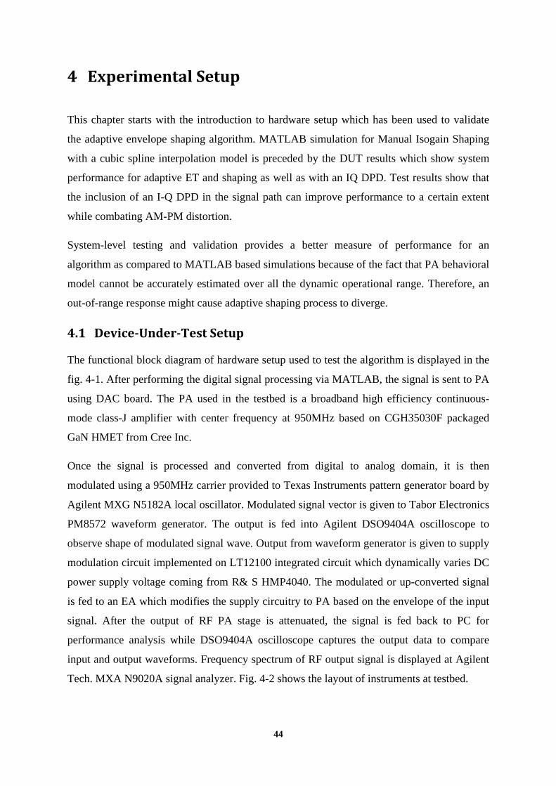
The functional block diagram of hardware setup used to test the algorithm is displayed in the

fig. 4-1. After performing the digital signal processing via MATLAB, the signal is sent to PA

using DAC board. The PA used in the testbed is a broadband high efficiency continuous-

mode class-J amplifier with center frequency at 950MHz based on CGH35030F packaged

GaN HMET from Cree Inc.

Once the signal is processed and converted from digital to analog domain, it is then

modulated using a 950MHz carrier provided to Texas Instruments pattern generator board by

Agilent MXG N5182A local oscillator. Modulated signal vector is given to Tabor Electronics

PM8572 waveform generator. The output is fed into Agilent DSO9404A oscilloscope to

observe shape of modulated signal wave. Output from waveform generator is given to supply

modulation circuit implemented on LT12100 integrated circuit which dynamically varies DC

power supply voltage coming from R& S HMP4040. The modulated or up-converted signal

is fed to an EA which modifies the supply circuitry to PA based on the envelope of the input

signal. After the output of RF PA stage is attenuated, the signal is fed back to PC for

performance analysis while DSO9404A oscilloscope captures the output data to compare

input and output waveforms. Frequency spectrum of RF output signal is displayed at Agilent

Tech. MXA N9020A signal analyzer. Fig. 4-2 shows the layout of instruments at testbed.

44

Figure 4-1: Block Diagram of Testbed

Figure 4-2: Instruments Layout

4.2 DUT Test Scenarios

The adaptive shaping algorithm discussed in 3.5.1 is tested with the hardware setup.

Following section presents the test results for an LTE 5MHz signal. In view of the project

objective to improve power efficiency using an envelope tracking RF PA, test scenario

includes following 03 configurations.

• Dynamic Supply RF amplification without Shaping function

• Envelope Shaping using adaptive technique

45

• Adaptive Envelope Shaping with an additional IQ DPD block to gain further benefits

in terms of linearity and reduced AM-PM distortion

A 5 MHz LTE signal is generated for testing using processing parameters defined in table 4-

1. Frequency spectrum of input signal shown in fig. 4-3 shows the power distribution over the

bandwidth before it is fed to envelope or signal path.

Figure 4-3: 5 MHz Input Signal Spectra

Table 4-1: Test Parameters

Parameter Values

No. of Samples 61440

Model Type Memory Polynomial

Local Oscillator Frequency 950 MHz

Baseband Bitrate 614.4 MHz

Lower Threshold Protection 0.4

In the sections 4.2.1 through 4.2.3 AM-AM characteristic curve, phase distortion at the

output, shaping curve for supply modulation and corresponding output spectra is presented.

Overall system performance will be analyzed consolidating results in section 4.3.

46

4.2.1 Dynamic Supply with No Shaping

Starting from a system which uses dynamic supply RF PA system based on the envelope of

the input signal with a shaping block, fig. 4-4 shows an input-output amplitude response

considering whole system in a black box approach. In this case, a dynamically varying

voltage signal is provided to RF PA exactly following the shape of input envelope without

any modification i.e. shaping function. The output curve shows nonlinearity which is a

typical characteristic of RF power amplifiers. In order to linearize magnitude response,

inverse distortion to the one shown in fig. 4-4 is pre-applied to the signal.

Figure 4-4: AM-AM Curve for Dynamic Supply Model without shaping function

Figure 4-5: AM-PM Response for Dynamic Supply Model with shaping function

47

Fig. 4-5 displays phase distortion caused by RF PA at the output. AM-PM distortion removal

is a significant challenge and it cannot be accomplished without the cost of added

computational complexity. Fig. 4-6 presents a clearer picture on why a dynamic supply

envelope tracking and shaping system performs better. Output signal frequency response of a

dynamic supply system with no shaping shows a considerable amount of power leakage into

sidebands. It will be compared with adaptive system in the following section.

Figure 4-6: RF Output Spectrum for Dynamic Supply Model without shaping function

4.2.2 Adaptive Shaping

Adaptive shaping algorithm updates polynomial parameters used for shaping function. PA

output is fed back to a shaping adaptation block which aims to minimize the error vector.

Following graphs exhibit an improvement in system performance. Fig. 4-7 shows that the

magnitude response of system is quite linear as compared to a no-shaping system. Contrary to

the improvement in AM-AM response, the adaptive shaping algorithm does not offer much

improvement in phase distortion as shown in fig. 4-8.

48

Figure 4-7: AM-AM Curve for Adaptive Shaping Model

Figure 4-8: AM-PM Response for Adaptive Shaping Model

Output frequency response of adaptive shaping system (Fig. 4-9) shows that ACLR values

are almost 10 dB better as compared to no-shaping approach. Although, the system operates

in a linear region, the PAE is consistent due to the use of a dynamic power supply, thus

highlighting the concept of optimal resource utilization.

49

Figure 4-9: RF Output Spectrum for Adaptive Shaping Model

Figure 4-10: Shaping Function curve for Adaptive Shaping Model

Fig. 4-10 is the supply modulation function which yields a back-off factor value against an

envelope sample and RF PA is then operated at optimum gain using that power supply.

4.2.3 Adaptive Shaping with IQ DPD

As discussed in previous chapters, phase distortion problem at the output can be overcome to

some extent using further linearization process. An IQ DPD block using memory polynomial

introduces an inverted estimation of RF PA output which in turn linearizes the output.

50

Figure 4-11: AM-AM Response for AS + IQ DPD

Introducing additional linearization techniques in signal path, improves AM-AM response

(Fig. 4-11) making it virtually linear. But the actual gain is in terms of a reduced phase

distortion for a complex RF signal. AM-PM response in fig. 4-12 shows a considerably less

input-output phase difference as compared to no-shaping technique and adaptive shaping

without an IQ DPD.

Figure 4-12: AM-PM Response for AS + IQ DPD

51

Figure 4-13: RF Output Spectrum for AS + IQ DPD

RF output spectra for test scenarios (Fig. 4-13) shows a significant ACLR improvement of 20

dB due to introduction of addition linearization of IQ DPD block. Shaping function for

adaptive shaping with IQ DPD shows a linear response (Fig. 4-14). Input signal envelope is

mapped to a back-off factor value to modify power supply level. Numerical values

representing gradual enhancement in system performance are shown listed in table 4-2.

Figure 4-14: Shaping Function curve for AS + IQ DPD

52

4.3 Performance Comparison

To analyze system performance in terms of PAE and linearity constraints such as ACLR,

values are listed in table 4-2. Taking a gradual approach, it can be seen that linearity

characteristics of RF PA output improve with a compromise on PAE percentage. An ACLR

improvement of 4.23 dB in lower and 5 dB in upper sideband of spectrum clearly signifies

that introducing a dynamic power supply introduces performance enhancement in linearity

constraints for communication standards. However, IQ DPD block with adaptive envelope

shaping truly remedies the challenge of useful power leakage into sidebands. Consequently,

PAE of the system improves from 42.8 % to 46.3 % but ACLR improvement of -44.55 dB

and -45. 79 dB is the actual gain in terms of performance.

Table 4-2: Performance Comparison

Linearization

Scheme

ACLR (dB) NMSE

(dB)

Pout

(dBm)

PAE

(%) Lower

Upper

LT

E 5

MH

z

No Envelope Shaping -23.10 -23.30 -17.8 27.5 49.2

Adaptive Shaping -27.33 -28.30 -27.4 29.7 42.8

AS+ IQ DPD -44.55 -45.79 -38.0 29.9 46.3

Improved value of NMSE from -27.4 dB to -38.0 defines the quality of estimation

considering a black box approach. For mobile applications, a lower threshold of -38 dB is

considered an acceptable solution with an output power of 26 dBm but inclusion of an IQ

DPD block in signal path adds computational complexity for power constrained applications

such as handheld mobile units.

4.3.1 Manual Shaping vs Adaptive Shaping

Table 4-3 lists a comparison between manual and adaptive shaping results. Manual shaping

uses a pre-characterization of PA output power vs gain for different supply voltage values. As

obvious from the results, overall system performance does not merit the inclusion of an

53

adaptive algorithm but in a real time system, static measurements of RF PA response are not

feasible. Moreover, PAs based on GaN HEMT transistors exhibit soft-compression in AM-

AM response when static PA characterization is performed [13]. Therefore, an adaptive

algorithm which iteratively converges to an optimal shaping function is the best solution in

terms of overall system performance.

Table 4-3: Manual vs Adaptive Shaping

Linearization

Scheme

ACLR (dB) NMSE

(dB)

Pout

(dBm)

PAE

(%) Lower Upper

5 M

Hz

LT

E Adaptive Shaping -33.00 -33.70 -27.7 33.3 47.6

Manual Shaping -34.2 -31.8 -26.2 33.1 51.9

4.3.2 Spline Interpolated Manual Shaping Model

Simulated results for a 5 MHz LTE signal are shown in figure 4-15 and 4-16 for 35.2667 dB

and 39.267 dB gain value respectively. Equation 3.20 transforms input power in dBm to

signal envelope value and corresponding power supply curve defines a back-off factor to

modulate power supply.

54

Figure 4-15: Gain vs Input Power (Targeted Gain = 35.2667dB)

Figure 4-16: Gain vs Input Power (Targeted Gain = 39.267dB)

55

By manually selecting the points where the isogain line intersects the power supply curves,

table 4-3 displays required supply voltage supply value. 0 dBm represents maximum input

power or maximum normalized envelope value.

Table 4-4: Input Envelope and Power Supply

Targeted Gain = 35.2667dB Targeted Gain = 39.267dB Input [dBm] Envelope |xBB| Supply [V] Input [dBm] Envelope

|xBB| Supply [V]

0 1 17.22 0 1 27.77 -1.664 0.8257 14.5 -0.666 0.9262 25.24 -4.073 0.6257 11.8 -1.807 0.8122 22.57 -7.559 0.4188 9.037 -3.247 0.6881 19.89

-5.001 0.5623 17.22 -7.678 0.4131 14.5

Envelope shaping function is created using data points presented in the table 4-3 with cubic

spline model. Input signal envelope or magnitude is the independent variable here whereas a

dynamic required value of power supply to PA is the dependent variable. Input provided to

cubic spline shaping model is a 5 MHz LTE signal. Since, the system has a restraint at

maximum available power supply for a certain isogain trajectory, therefore all the values of

input signal envelope higher than maximum system limit are being considered to be

amplified with the maximum power supply which is 17.22V for a targeted gain of

35.2667dB.

56

Figure 4-17: Shaping Model (35.2667dB Gain)

Figure 4-18: Shaping Model (39.267dB Gain)

The maximum optimal power supply at the peak of input signal envelope in shaping curve

represents the system limit according to the isogain line. Meanwhile, the lower limit

57

corresponds to the fact that dynamic power supply cannot go as low as 0 V but has to pre-

assign a threshold value of power supply to use for input with low RF power.

Cubic spline model can be incorporated into adaptive envelope shaping algorithm to replace a

polynomial model to improve estimation accuracy. However, computational complexity may

turn out to be a limit because unlike polynomial interpolation which uses a single function

and the only controllable parameter is polynomial order or the no. of coefficients, Spline

model in general uses a an independent function between each set of interpolation points. An

adaptive cubic spline model in particular has to calculate 3rd order equations for estimating

output between 2 consecutive points and adaptation further adds to computational cost at

digital signal processing stage.

58

5 Conclusion

Before starting to look for an alternative approach to fixed DC power supply RF PAs for high

PAPR signals, it was very critical to establish a problem statement. Analysis of the

performance requirements for modern communication standards lead to the idea of a dynamic

supply power amplification system where only the need based power was to be consumed

ideally.

After identification of the problem, basic PA principle is described linking to performance

metrics for transmission quality. Along comes the need to manipulate a conventional system

architecture where a modulated baseband signal is fed to an amplifier and transmitted using a

fixed amount of drain supply to PA irrespective of the magnitude of the input to the system.

With PA itself being a non-linear device, it has been deemed as a poor approach when the

overall system resources are considered. Moreover, with the advent of various handheld

devices which have limited power at their disposal, different tracking techniques for the

envelope of input have offered promise.

Average power tracking and Envelope tracking improve a system’s PAE. The core concept is

to dynamically change which is being fed to PA as power supply based on the input signal.

This variation of drain voltage is instantaneous, at sub-sample level in case of envelope

tracking. With the use of envelope tracking strategy, the conventional forward path to feed

baseband signal to PA divides into two paths with separate signal processing modules. Signal

is fed to PA on ‘Signal Path’ with an additional forward path called ‘Envelope Path’ includes

magnitude calculation of input signal before it controls an additional amplifier known as EA.

After gauging the system behavior and forming an input-output model, a shaping block is

introduced in envelope path. Starting with a memoryless power series, the algorithm then

went on to incorporate memory effect. These linearization strategies are studied, and then

tested on a testbed with a DUT. The ability to test the algorithm on a hardware system has

provided an insight to responses to behavioral model which are challenging to simulate on a

software platform.

Shaping function in the algorithm has been based on polynomial model. A trivial alternative

which saves system resources in terms of computational complexity of algorithm is to use to

LUT(s). Instead of performing polynomial interpolation for each block of data, a lookup table

59

offer speed by pre-allocating the inputs to supply modulation circuitry. However, as

established in chapter 3, Spline Interpolation can be a method which offers increased

stability. For an adaptive envelope tracking and shaping block which uses a feedback from

PA output, a cubic spline model may offer improvement in performance. Cubic Spline model

is developed for a manual (by-hand) shaping function. Picking up a set of points from a data

pool which contains input signal envelope and corresponding power supply values for an

LTE 5MHz, shaping curves for different values of targeted output gain are included.

Presented in chapter 4, the results show that proposed adaptive shaping algorithm’s enhances

system spectral characteristics i.e. ACLR is reduced when compared to a manual shaping

simulation. The results improve further when a LUT is introduced in shaping function block.

The most significant improvement in overall system performance is achieved when a

linearization strategy is employed for signal path as well. By introducing a DPD in signal

path, the AM-PM distortion is reduced which improves system performance.

60

Bibliography

[1] Baker, S., “ET101An Introduction to Envelope Tracking for RF Amplifiers,” white paper, November 2011.

[2] The Mobile Economy Report, GSM Association, 2014.

[3] The Tauri Group, State of the Satellite Industry Report, Technical Report, Satellite Industry Association, May 2014.

[4] Jean-Didier Gayrard, Cédric Baudoin, Christine Miquel, Michel Sghedoni, “Wireless Communications for Satellite Formation Flying,” July 2006.

[5] Joel Vuolevi and Timo Rahknonen, “Distortion in RF Power Amplifiers.” Artech House, 2003. ISBN:1580535399.

[6] Zhangcang Wang. ‘Envelope Tracking Power Amplifiers for Wireless Communications’. Artech House, 2014.

[7] Pere L. Gilabert, Gabriel Montoro, “Digital Predistortion for Envelope Tracking Amplifiers,” International Microwave Symposium, June 2013.

[8] Pere L. Gilabert, Gabriel Montoro, “Design of Adaptive Digital Predistorter Linearizers for Envelope Tracking Power Amplifiers,” Workshop on Signal Processing and Amplifiers 2012.

[9] Schreurs, D., M´airt´ın O’Droma, Anthony A. Goacher, Michael Gadringer, “RF Power Amplifier Behavioral Modeling,” The Cambridge RF and Microwave Engineering Series. Cambridge University Press, 2009. ISBN: 9780521881739.

[10] Joel Vuolevi and Timo Rahknonen. ‘Distortion in RF Power Amplifiers’. Artech House, 2003. ISBN: 1580535399.

[11] R. Neil Braithwaite. ‘Principles and Design of Digital Predistortion’. In Fa-Long Luo, editor, Digital Front End in Wireless Communications and Broadcasting—Circuits and signal Processing, chapter6. Cambridge University Press, 2011. ISBN: 9781107002135.

[12] Pedro M. Sousa, “Digital Predistortion of Wideband Satellite Communication Signals with Reduced Observational Bandwidth and Reduced Model Order Complexity,” MAST, UPC, Oct 2014.

[13] J. C. Pedro, L. C. Nunes, P. M. Cabral, “Soft compression and the origins of nonlinear behavior of GaN HEMTs,” in Microwave Conference (EuMC), 2014 44th European, Oct 2014, pp. 1297–1300.

[14] R.Wu, Y.-T. Liu, J. Lopez, C. Schecht, Y. Li, and D. Lie, “High-Efficiency Silicon-Based Envelope-Tracking Power Amplifier Design With Envelope Shaping for Broadband

61

Wireless Applications,” Solid-State Circuits, IEEE Journal of, vol. 48, no. 9, pp. 2030–2040, Sept 2013.

[15] D. Kim, D. Kang, J. Choi, J. Kim, Y. Cho, and B. Kim, “Optimization for Envelope Shaped Operation of Envelope Tracking Power Amplifier,” Microwave Theory and Techniques, IEEE Transactions on, vol. 59, no. 7, pp. 1787–1795, July 2011.

[16] T. Rautio, H. Harju, S. Hietakangas, and T. Rahkonen, “Envelope tracking power amplifier with static predistortion linearization,” Int. Journal of Circuit Theory and Applications, vol. 37, no. 2, pp. 365–375, 2009.

[17] Lucyszyn, S., “Power-Added Efficiency Errors with RF Power Amplifiers,” International Journal of Electronics, Vol. 82, No. 3, March 1997, pp. 303-312.

[18] Cripps, S.C., RF Power Amplifiers for Wireless Communications, Norwood, MA: Artech House, 2006.

[19] Kim, I., et al., “High-Efficiency Hybrid EER Transmitter Using Optimized Power Amplifier,” IEEE Transactions on Microwave Theory and Techniques, Vol. 56, No. 11, 2008, pp. 2582-2593.

[20] Hanington, G., et al., “High Efficiency Power Amplifier Using Dynamic Power-Supply Voltage for WCDMA Applications,” IEEE Transactions on Microwave Theory and Techniques, Vol. 47, No. 8, August 1999, pp. 1471-1476.

[21] Hoversten, J.Z., M.N. Popovic, and D. Maksimovic, “Power Amifier to Envelope Modulator Interconnects for Envelope Tracking Transmitters,” Intellectual property disclosure, University of Colorado at Boulder, Boulder, CO, April 2009.

[22] Aitto-oja, T., “High Efficiency Envelope Tracking Supply Voltage Modulator for High Power Base Station Amplifier Applications,” 2010 IEEE MTT-S International Microwave Symposium Digest (MTT), 2010, pp.668-671.

[23] Hubbard, M., “Taming the smartphone Power Consumption Vicious Cycle,” Microwave Journal, November 2012, pp. 92-96.

[24] Mike Renfro, “Programs for Natural Cubic Spline Interpolation,” November 2004.

[25] Wang, K., “A Study of Cubic Spline Interpolation,” Rivier Academic Journal, Vol. 9, No. 2, 2003.

[26] Huseyin Ozdemir, “Comparison of linear, cubic spline and akima interpolation methods,” August 2007.

62