master thesis christian lunden - uio
TRANSCRIPT
UNIVERSITY OF OSLODepartment of Informatics
Evaluation ofDifferent SANTechnologies forVirtual MachineHosting
Oslo University College
Master thesis
Christian Lunden
May 18, 2009
Evaluation of different SAN technologies
for Virtual machine hosting
Christian Lunden
2009-18-05

Abstract
This thesis covers a problem which companies faces every day: Finding a Storage AreaNetwork(SAN) solution that tackles the rising demands from users and their software and whenworking with virtualization environments. In this paper it will be showed a way to investigateand identify, from a selection of SAN technologies, which is the most efficient and optimal basedon scenarios that fits real life experiences. The approach taken was to create an experimentalsetup in a controlled environment that fits real life experience. The benchmark tool bonnie++was used to simulate activity and interpreted by an analysis script tool developed by the author.Distributed Replicated Block Device(DRBD), Network File System(NFS), Parallel Virtual FileSystem(PVFS), Internet SCSI(ISCSI) and ATA over Ethernet(AoE) are the SAN technologieswhich will be evaluated and discussed. The optimal SAN technologies will be chosen based ona certain criterias such as raw performance and stability.

2

Acknowledgements
I would first of all like to thank my supervisor Kyrre M. Begnum without whom I would nevermade it this far. Thanks for all the support and motivational talks we have had from the startto the finish line. My thanks also to the system administrator at ABC Startsiden Ingard Mev̊agand his crew for providing me with equipment and a good working environment. My familyhas been very important to me during this process. Especially my mom with her love and careduring these past few months and dad with his words of wisdom and for always managing to getme back on my feet when I hit the wall as in a figure of speech. I would also like to extend mygratitude to Professor Mark for providing us with this Master course, giving me the opportunityto work with technology I love and challenges that I will face in a working environment, so thatI will be prepared. Finally, I want to thank my classmates for two years of companionship thathas given me many good memories that will last a lifetime.
3

4

Contents
1 Introduction 111.1 Motivation . . . . . . . . . . . . . . . . . . . . . . . . . . . . . . . . . . . . . . . 111.2 Problem Statement . . . . . . . . . . . . . . . . . . . . . . . . . . . . . . . . . . . 121.3 Approach . . . . . . . . . . . . . . . . . . . . . . . . . . . . . . . . . . . . . . . . 12
1.3.1 Survey . . . . . . . . . . . . . . . . . . . . . . . . . . . . . . . . . . . . . . 121.3.2 Comparative study . . . . . . . . . . . . . . . . . . . . . . . . . . . . . . . 12
1.4 Thesis Outline . . . . . . . . . . . . . . . . . . . . . . . . . . . . . . . . . . . . . 13
2 Background 152.1 Storage Area Network technologies . . . . . . . . . . . . . . . . . . . . . . . . . . 15
2.1.1 Network-attached storage . . . . . . . . . . . . . . . . . . . . . . . . . . . 152.1.2 Network File System . . . . . . . . . . . . . . . . . . . . . . . . . . . . . . 162.1.3 NAS vs SAN . . . . . . . . . . . . . . . . . . . . . . . . . . . . . . . . . . 16
2.2 iSCSI . . . . . . . . . . . . . . . . . . . . . . . . . . . . . . . . . . . . . . . . . . 162.2.1 Architecture . . . . . . . . . . . . . . . . . . . . . . . . . . . . . . . . . . 16
2.3 DRBD . . . . . . . . . . . . . . . . . . . . . . . . . . . . . . . . . . . . . . . . . . 172.4 Pvfs . . . . . . . . . . . . . . . . . . . . . . . . . . . . . . . . . . . . . . . . . . . 18
2.4.1 Architecture . . . . . . . . . . . . . . . . . . . . . . . . . . . . . . . . . . 192.5 ATA over Ethernet . . . . . . . . . . . . . . . . . . . . . . . . . . . . . . . . . . . 19
2.5.1 Architecture . . . . . . . . . . . . . . . . . . . . . . . . . . . . . . . . . . 192.6 Virtualization . . . . . . . . . . . . . . . . . . . . . . . . . . . . . . . . . . . . . . 20
2.6.1 Virtualization and networked storage . . . . . . . . . . . . . . . . . . . . . 202.6.2 Xen . . . . . . . . . . . . . . . . . . . . . . . . . . . . . . . . . . . . . . . 212.6.3 Factors that could affect performance . . . . . . . . . . . . . . . . . . . . 22
2.7 bonnie++ . . . . . . . . . . . . . . . . . . . . . . . . . . . . . . . . . . . . . . . . 22
3 Methodology 253.1 Analysis Tool . . . . . . . . . . . . . . . . . . . . . . . . . . . . . . . . . . . . . . 25
3.1.1 Input . . . . . . . . . . . . . . . . . . . . . . . . . . . . . . . . . . . . . . 253.1.2 Usage . . . . . . . . . . . . . . . . . . . . . . . . . . . . . . . . . . . . . . 26
3.2 Experimental Setup . . . . . . . . . . . . . . . . . . . . . . . . . . . . . . . . . . 273.2.1 Base tests . . . . . . . . . . . . . . . . . . . . . . . . . . . . . . . . . . . . 283.2.2 non-Base tests . . . . . . . . . . . . . . . . . . . . . . . . . . . . . . . . . 29
3.3 Output . . . . . . . . . . . . . . . . . . . . . . . . . . . . . . . . . . . . . . . . . 293.4 Analysis . . . . . . . . . . . . . . . . . . . . . . . . . . . . . . . . . . . . . . . . . 29
5

4 Results 314.1 Explanation of output in tables . . . . . . . . . . . . . . . . . . . . . . . . . . . . 314.2 Keeper basetest . . . . . . . . . . . . . . . . . . . . . . . . . . . . . . . . . . . . . 314.3 Nexus basetest . . . . . . . . . . . . . . . . . . . . . . . . . . . . . . . . . . . . . 354.4 Nexus with one VM . . . . . . . . . . . . . . . . . . . . . . . . . . . . . . . . . . 394.5 Iscsi basetest . . . . . . . . . . . . . . . . . . . . . . . . . . . . . . . . . . . . . . 424.6 Iscsi 3of3 test . . . . . . . . . . . . . . . . . . . . . . . . . . . . . . . . . . . . . . 464.7 NFS basetest . . . . . . . . . . . . . . . . . . . . . . . . . . . . . . . . . . . . . . 504.8 NFS 3of3 test . . . . . . . . . . . . . . . . . . . . . . . . . . . . . . . . . . . . . . 544.9 DRBD basetest . . . . . . . . . . . . . . . . . . . . . . . . . . . . . . . . . . . . . 584.10 DRBD 3of3 test . . . . . . . . . . . . . . . . . . . . . . . . . . . . . . . . . . . . . 614.11 Summary . . . . . . . . . . . . . . . . . . . . . . . . . . . . . . . . . . . . . . . . 64
5 Discussion 715.0.1 The Process . . . . . . . . . . . . . . . . . . . . . . . . . . . . . . . . . . . 715.0.2 The Results . . . . . . . . . . . . . . . . . . . . . . . . . . . . . . . . . . . 72
6 Conclusion 75
Appendices 79
A Selected bonnie++ output files 81
6

List of Figures
3.1 Figure of the lab setup . . . . . . . . . . . . . . . . . . . . . . . . . . . . . . . . . 273.2 experimental setup . . . . . . . . . . . . . . . . . . . . . . . . . . . . . . . . . . . 28
4.1 keeper put block . . . . . . . . . . . . . . . . . . . . . . . . . . . . . . . . . . . . 344.2 keeper get block . . . . . . . . . . . . . . . . . . . . . . . . . . . . . . . . . . . . 344.3 keeper seeks . . . . . . . . . . . . . . . . . . . . . . . . . . . . . . . . . . . . . . . 354.4 Nexus novm putblock . . . . . . . . . . . . . . . . . . . . . . . . . . . . . . . . . 374.5 Nexus novm getblock . . . . . . . . . . . . . . . . . . . . . . . . . . . . . . . . . . 374.6 Nexus novm seeks . . . . . . . . . . . . . . . . . . . . . . . . . . . . . . . . . . . 374.7 Nexus onevm put block . . . . . . . . . . . . . . . . . . . . . . . . . . . . . . . . 414.8 nexus onevm get block . . . . . . . . . . . . . . . . . . . . . . . . . . . . . . . . . 414.9 iscsi putblock . . . . . . . . . . . . . . . . . . . . . . . . . . . . . . . . . . . . . . 444.10 iscsi getblock . . . . . . . . . . . . . . . . . . . . . . . . . . . . . . . . . . . . . . 444.11 iscsi seeks . . . . . . . . . . . . . . . . . . . . . . . . . . . . . . . . . . . . . . . . 454.12 iscsi 3of3 putbl . . . . . . . . . . . . . . . . . . . . . . . . . . . . . . . . . . . . . 484.13 iscsi 3of3 getblock . . . . . . . . . . . . . . . . . . . . . . . . . . . . . . . . . . . 484.14 iscsi 3of3 seeks . . . . . . . . . . . . . . . . . . . . . . . . . . . . . . . . . . . . . 494.15 NFS base putblock . . . . . . . . . . . . . . . . . . . . . . . . . . . . . . . . . . . 524.16 NFS base getblock . . . . . . . . . . . . . . . . . . . . . . . . . . . . . . . . . . . 524.17 NFS base seeks . . . . . . . . . . . . . . . . . . . . . . . . . . . . . . . . . . . . . 534.18 NFS 3of3 putblock . . . . . . . . . . . . . . . . . . . . . . . . . . . . . . . . . . . 564.19 NFS 3of3 getblock . . . . . . . . . . . . . . . . . . . . . . . . . . . . . . . . . . . 564.20 NFS 3of3 seeks . . . . . . . . . . . . . . . . . . . . . . . . . . . . . . . . . . . . . 574.21 DRBD basetest putblock . . . . . . . . . . . . . . . . . . . . . . . . . . . . . . . . 594.22 DRBD basetest getblock . . . . . . . . . . . . . . . . . . . . . . . . . . . . . . . . 604.23 DRBD basetest seeks . . . . . . . . . . . . . . . . . . . . . . . . . . . . . . . . . . 604.24 DRBD 3of3 putblock . . . . . . . . . . . . . . . . . . . . . . . . . . . . . . . . . . 634.25 DRBD 3of3 getblock . . . . . . . . . . . . . . . . . . . . . . . . . . . . . . . . . . 634.26 DRBD 3of3 seeks . . . . . . . . . . . . . . . . . . . . . . . . . . . . . . . . . . . . 634.27 Performance Summary Mean . . . . . . . . . . . . . . . . . . . . . . . . . . . . . 654.28 Performance Summary Range . . . . . . . . . . . . . . . . . . . . . . . . . . . . . 664.29 Performance Summary Mean 3VMs . . . . . . . . . . . . . . . . . . . . . . . . . . 674.30 Performance Summary Range 3VMs . . . . . . . . . . . . . . . . . . . . . . . . . 68
7

8

List of Tables
4.1 Table of keeper basetest . . . . . . . . . . . . . . . . . . . . . . . . . . . . . . . . 324.2 Table of nexus basetest . . . . . . . . . . . . . . . . . . . . . . . . . . . . . . . . 354.3 Table from Nexus onevm . . . . . . . . . . . . . . . . . . . . . . . . . . . . . . . 394.4 Table of iscsi basetest . . . . . . . . . . . . . . . . . . . . . . . . . . . . . . . . . 424.5 Table of iscsi 3of3 test . . . . . . . . . . . . . . . . . . . . . . . . . . . . . . . . . 464.6 Table of NFS basetest . . . . . . . . . . . . . . . . . . . . . . . . . . . . . . . . . 504.7 Table of NFS 3of3 test . . . . . . . . . . . . . . . . . . . . . . . . . . . . . . . . . 544.8 Table of DRBD basetest . . . . . . . . . . . . . . . . . . . . . . . . . . . . . . . . 584.9 Table of DRBD 3of3 test . . . . . . . . . . . . . . . . . . . . . . . . . . . . . . . . 614.10 Table of Summary Results Mean Basetest . . . . . . . . . . . . . . . . . . . . . . 644.11 Table of Summary Results Range Basetest . . . . . . . . . . . . . . . . . . . . . . 654.12 Table of Summary Results Mean 3 VMs test . . . . . . . . . . . . . . . . . . . . 674.13 Table of Summary Results Range 3 VMs test . . . . . . . . . . . . . . . . . . . . 68
9

10

Chapter 1
Introduction
1.1 Motivation
Companies today need storage possibilities like Storage Area Network(SAN). There is a risingdemands from stakeholders in major corporations to smaller businesses that have both systemadministrators and a large network of employees/clients. This technology adds some degree ofcertainty of their work not being lost when computers crash due to hardware or software failure,and for system administrators to gain a better way of handling backup situations.
Finding one SAN solution that is the best in correspondence to the setup of the company isnot easy. Obstacles like what type of operating system they are using, how much money theywould like to invest and how the technology they are interested in, fits in with the other typeof software they are using.
There is a large variety of SAN technologies to choose from in the market today. This is amany-to-many problem which will require testing to figure out what type of SAN that is needed.Setup of the companies computer system would respond differently for each of the technologieswe can choose from.
A common way of testing out whether the SAN technology is a good pick for the systemof a company is to combine SAN with Virtualization. This way we can perform some stresstesting and find out its strengths and weaknesses. Several scenarios should be made since thetechnology itself might respond differently depending on the setup of the system.
Companies needs their workplace to operate efficiently and have a secure way of backing upso that there is a way to restore when important data is lost. Therefore, the descision on whatSAN that is suited for their systems, should be determined based on a number of dimensions.
In stress testing the SAN technology there are different terms that are important. Two fac-tors that distinguishes themselves from the others are performance and stability. These factorsare fundamental for checking how well the SAN technology works.
The combination with SAN technology and Virtualization is a good way to use these kindof pressures tests. Since we can scale up several clients which will take use of the SAN technol-ogy. Moreover, adding this to valid scenarios could help in finding the best SAN solution for acompany.
11

1.2 Problem Statement
The following problem statement was chosen for this project after going through motivationalpointers and formulate it in such a way that it could be possible to find a solution.
How to investigate and identify a combination with SAN technologies and Virtualization thatis efficient and optimal?
Investigate and identify means here experimenting in an controlled environment and performanalysis based on these results. SAN technologies Storage Area Network, a different set oftechnologies used for storing and backing up files on a system. Virtualization - Enterprise levelsoftware that is commonly known and used for setting up larger networking systems. Efficientand optimal draws it meaning from a benchmarking point of view. From data gathered fromexperiments that are analysed there should be possible to find whether the solution is better orworse.[2]
1.3 Approach
There are several ways to approach the problem for this project. In this section we will lookat some of the most used ways to handle these kind of problems, and why this approach waschosen for this problem.
1.3.1 Survey
Studying previous work done with SAN technology and benchmark testing could provide withenough data to calculate some predicaments and conclude whether one of the SAN solutions isbetter than the other. On the other hand this could give a wrong picture of actual performancefor the SAN since not all combinations would be analysed by each other.
1.3.2 Comparative study
This approach that requires cooperation with several companies to gain access to their pro-duction environment. Furthermore, we need to be allowed to use their equipment in order toperform measurements, so that there is possible to compare results. A problem might occurwith this approach since it can not be done in an controlled environment. Companies havedifferent set ups and hardware solutions. In terms of newer technology it would also be hard torun and test them on the current system of the company. Since we will not be able to alter theircurrent configurations on the system and have no other option than to use what they alreadyhave. Realistic speaking, time would be a problem for this type of approach, since it wouldbe problems visiting enough companies to conduct the project.Especially considering that theyshould be within the boundaries of a controlled experiment.
The chosen approach is interesting for system administrators in view of newer technology,reading about the results could also encourage them to test this technology at their own com-pany. They could also be interested in the different scenarios that will be used in this approachas well as the analysis in terms of saleability Since it will require a large number of clients togive enough pressure on the technology itself to determine its performance.
12

1.4 Thesis Outline
This chapter contains the motivational pointers for this project and how the problem statementgot formulated. Chapter 2.1 explains in detail the different technologies used during this project,the SAN technologies that are to be tested and the tools used for measuring and fully test themout. The methodology of this project, what kind of experimental setup and lab equipment usedduring this project is mentioned in chapter 3. Results will be displayed in chapter 4 with a briefoverview and fully explained descriptive statistics for the data that was measured. Chapter 5will discuss these results and based on these discussions find out which technology that performsbetter or worse which we will conclude in the last chapter.
13

14

Chapter 2
Background
The previous chapter contained the motivation and formulated the problem statement. Fur-thermore, some different approaches were mentioned for giving solutions or answers to thisstatement. In this chapter we will review the background literature for the different technolo-gies used in this project and briefly describe different factors that could affect the results in theend.
2.1 Storage Area Network technologies
Demands for storage solutions has increased in recent years. Companies used to have data onservers that were connected to the Local Area Network(LAN) or Wide Area Network depend-ing on the set-up of their system. On this server canalization of traffic such as data transfersand backing up the data would take place. Today SANs have taken over as a solution.[9]SANscreate a pool of storage devices, where they are linked together, so that users can connect andaccess the data directly over the network. In addition to reducing bandwidth load, it has betterstorage management and more fault tolerance. Moreover, SANs have the ability to transmitdata at high speeds over great distance when used in combination with fibre channel technology.
However, there are complications integrating the fibre channel technology with hardwaretechnologies, which is often upgraded. Hence, there have been vendors working on ways to linkSAN technologies over Ethernet and other networking technologies. The solution vendors havefound has evolved SAN and made it possible for this technology to work together with otherprotocols, and has become multi protocol capable. Furthermore, towards the simplification ofthe SAN infrastructure, technologies that were competing with SAN for floor space can nowwork together in a single machine.
2.1.1 Network-attached storage
Network-attached storage(NAS) is also a commonly used storage technology. The way thistechnology works is that it is a computer connected to the network, with installed NAS soft-ware on it. This unit can provide with file-based storage services for clients connected to thenetwork. A NAS storage contains an engine that implements file services which is possible whenusing access protocols such as NFS or CIFS. When more hard disk storage space is needed ona network that already utilize servers, NAS is allowed to add this without having to shut theservers down for maintenance and upgrades.
15

NAS is not an integral part of the server, but a device that delivers data to the user whilethe server handles all processing of data. This device does not need to be located within theserver but can be placed anywhere in the LAN. It is also possible to make them up of multiplenetworked NAS devices. These units uses Ethernet and file-based protocols to communicate,which differs from SANs use of Fibre Channel and block-based protocols for communicating.This type of storage gives acceptable performance and security, and provides with less expenseswhen being implemented to the servers because of the usage of Ethernet adapters instead ofFibre Channel adapters. [7]
2.1.2 Network File System
The Network File System(NFS) is a technology that operates on a client to server level. Itis designed to let users(clients) view and optionally store and update files on a remote com-puter. However, for allowing this the user needs to have an NFS client and the remote computerneeds the NFS server. These applications allows for the NFS to work over the TCP/IP protocol.
Moreover, NFS server provides the possibility of organizing important files on a centralizedlocation, allowing authorized users continuous access. NFS has currently two versions that areused. NFS version 2(NFSv2), which is supported by many operating systems and has beenaround for several years. NFS version 3(NFSv3) is the second version. It has more featuresthan NFSv2 like including a variable file handle size and better error reporting.
2.1.3 NAS vs SAN
We have looked through two popular choices when it comes to storage technology. Both havedifferent strengths and weaknesses which makes none of them the ”best” choice. Compared toSAN, NAS provides with a storage and file system SAN, on the other hand, only provides withstorage technology and let the matter of the file system go to the clients side. Both work withvirtualization like Xen, because Xen can access the virtual machines disk either like a file or ablock device. Example below is a line from a Xen configuration file, where you can specify thelocation of the image you want to use.
disk = [ ’file://home/christian/disk.img,hda1,w’ ]
2.2 iSCSI
Internet SCSI, or iSCSI has emerged as a protocol and looked upon as a solution for theincreased demands in the industry. Compared to Fibre Channel usage within SANs, iSCSI hasa few advantages that gives them a growth in the market.
2.2.1 Architecture
The iSCSI protocol has the ability to map over TCP/IP and enable access to TCP/IP networksover Ethernet.[11] In the mapping process SCSI block oriented storage data will be transferedwhich will enable the storage devices to work over Ethernet. There are many reasons for itspopularity, reduced cost and the possibility to achieve a uniformed network infrastructure whendeploying iSCSI protocol over a Gigabit Ethernet. This allows for the storage to be reachedover a larger area, since there is usually a physically restriction to a limited environment in a
16

traditional storage system like Fibre Channel for instance.
Another positive point is the availability of inexpensive software implementations of theiSCSI protocol, which could allow use of compelling platforms in a iSCSI deployment. On theother hand, the iSCSI-based storage is not without challenges. One of the main challenges thatfaces iSCSI is the issues in the network traffic between an initiator and a target that are far apartfrom each other[12]. An initiator serves the same purpose as a SCSI bus adapter would, exceptinstead of being physically attached it uses SCSI commands over the network. The target, onthe other hand, represents the location for the iSCSI server, where storage resources are madeavailable for the users. If compared to other existing technologies such as Fibre Channel, thereare improvements to be made in terms of efficiency and performance. Moreover, networkingtechnology between initiator and target can be diverse and heterogeneous. This could causechanges so that packets suffers from long delay, loss and retransmission.
2.3 DRBD
DRBD which stands for Distributed Replicated Block Device is an implementation in form ofa Linux kernel module providing a two-node high availability(HA) cluster. It was developed byPhilipp Reisner and Lars Ellenberg and their team at LINBIT. The purpose of this technologyis to keep a high data availability up for a company which also includes when a system breakscompletely down. [6].
Architecture
As already mentioned DRBD works as an Linux kernel module. This technology provides ablock device driver for the kernel. For each of these cluster nodes, this driver will be in controlof a ”real” block device that holds a replication of the systems data. Operations concerningread will be run locally while writing will be transmitted to the other nodes in the HA cluster.
The transport layer chosen for this technology is TCP, mostly because of it is available forkernel modules. Furthermore, the choice of this layer was based on its solution to two basicproblems, the packet recording and the flow control. This has simplified the development, how-ever, it has also brought limitations for the DRBD-based clusters to two-nodes.
Moreover, the design of the technology at its current state, allows for only one node tomodify the replicated storage. However, it is possible to change roles of the nodes but not dataat a concurrent rate on both of the nodes. There are two roles which is possible for each of thenodes in this DRBD architecture, primary or secondary state.
Write access is only granted to applications in the primary state of a given device. Thisonly applies for one device in a connected device pair, if you try to apply it for both they willbreak up the connection and form their independent degraded clusters. Assigning these rolesare usually managed by a cluster management software, Heartbeat and Failsafe.
#/etc/drbd.confglobal {usage-count yes;
17
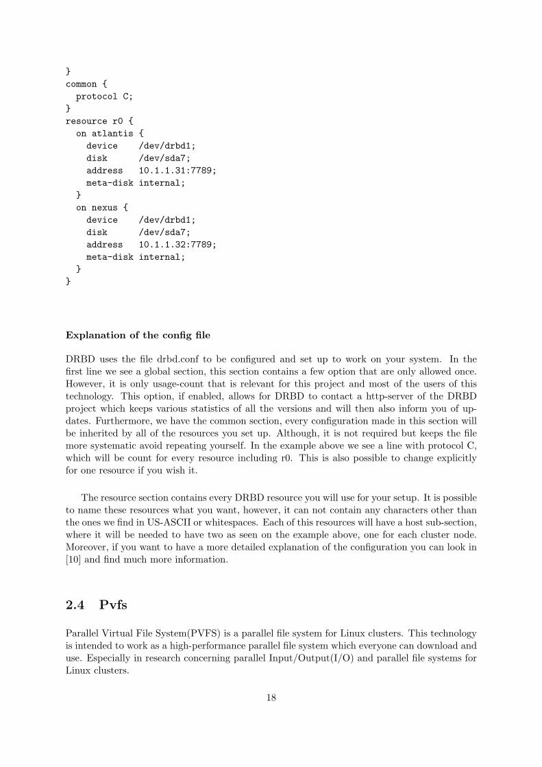
}common {protocol C;
}resource r0 {on atlantis {device /dev/drbd1;disk /dev/sda7;address 10.1.1.31:7789;meta-disk internal;
}on nexus {device /dev/drbd1;disk /dev/sda7;address 10.1.1.32:7789;meta-disk internal;
}}
Explanation of the config file
DRBD uses the file drbd.conf to be configured and set up to work on your system. In thefirst line we see a global section, this section contains a few option that are only allowed once.However, it is only usage-count that is relevant for this project and most of the users of thistechnology. This option, if enabled, allows for DRBD to contact a http-server of the DRBDproject which keeps various statistics of all the versions and will then also inform you of up-dates. Furthermore, we have the common section, every configuration made in this section willbe inherited by all of the resources you set up. Although, it is not required but keeps the filemore systematic avoid repeating yourself. In the example above we see a line with protocol C,which will be count for every resource including r0. This is also possible to change explicitlyfor one resource if you wish it.
The resource section contains every DRBD resource you will use for your setup. It is possibleto name these resources what you want, however, it can not contain any characters other thanthe ones we find in US-ASCII or whitespaces. Each of this resources will have a host sub-section,where it will be needed to have two as seen on the example above, one for each cluster node.Moreover, if you want to have a more detailed explanation of the configuration you can look in[10] and find much more information.
2.4 Pvfs
Parallel Virtual File System(PVFS) is a parallel file system for Linux clusters. This technologyis intended to work as a high-performance parallel file system which everyone can download anduse. Especially in research concerning parallel Input/Output(I/O) and parallel file systems forLinux clusters.
18

2.4.1 Architecture
Primary goal of the PVFS is to provide high-speed access to file data for parallel applications.Furthermore, PVFS provides with features like user controlled striping of data across diskson different I/O nodes, allowing existing data to operate on PVFS without recompiling andconsistent name space.
The PVFS design is a client-server system with multiple servers, which are called I/O dae-mons. I/O daemons are on separate nodes in the cluster. These I/O nodes have disks attachedto them, which the PVFS files will be striped across over. Moreover, PVFS also has a man-ager daemon which handles metadata operations like permissions in creating, open, close andremove of files. The manager itself does not involve in read/write operations, the client andI/O daemons handles all file operations. The different kind of operators such as the clients, I/Odaemons and manager do not have to be on separate machines. Although, it might prove to bebetter in terms of performance to keep them apart.[8]
PVFS has no kernel modifications or modules are needed to install or operate this system,which makes it primarily a user-level implementation. Furthermore, PVFS uses TCP for thecommunication that goes on internally, which makes it not dependent on any specific message-passing library.
2.5 ATA over Ethernet
The ATA over Ethernet(AoE) is an open standard based protocol which allows for clients toaccess disk drives directly over the network that are attached to a client host. This could eitherbe a web, mail or cluster server. This protocol has simple implementation that can make thecost of AoE server to be very low.
2.5.1 Architecture
In this protocol there are two classes of messaging, ATA and Config/Query, which we will dis-cuss a bit more in detail as well as the shared common header they have. The common headerworks in such a way that it is possible to send messages between client hosts and AoE servers.It consists of four functions which we will mention now in order. First, it grants the possibilityto correlate responses with requests. Providing a way to to discover the Ethernet address of anAoE server when it is placed in rack storage blades, is the second function. Third, is that thecommon header can identify requests from responses. The last function of the common headeris that it contains error information.
The Advanced Technology Attachment(ATA) is a standard that evolved since the early1980‘s from both the ST506 interface and the Western Digital 1010 disk controller chip. Thesechips had a set of registers which held the information of cylinder, track and sector. Fur-thermore, there was a also a command register that used to initiate data transfers by writingoperational codes to it. A status and error register reported if it was a successful or unsuccessfulcompletion of the command. Todays ATA standard covers both the physical connections to thedrive and the logical interface. Its messages contain requests and responses which will performATA transactions. In these transactions, there are three possibilities: no transfer of data, datais being written to disk, or data is read from disk. This mechanism with ATA messages simplyexports ATA interface on AoE servers to the client hosts. For more detailed information on theheader of these messages you can read more in [4].
19

The Config/Query messages is the second class of AoE messages. There are two ways to setthe config data. One way is to set the config memory to a value only if the current config datais zero length, which can be done by a set request. However, if the config memory already hasnon-zero length data, the set request fails. Another option is to force the AoE server to set theconfig memory. Config values intended for the data can be zero length, allowing the config datato be reset. The contents in Query messages can be used to optionally match against the storedconfig information. There are three different ways of querying for the data. First approach isthat the config data can be unconditionally read. Another way is that the config data can bereturned. Although, this is only possible if the query data matches the prefix of the config onthe AoE server. What is meant by this is that the query has a number of bytes, that is less thanor equal to the length of the data in the server. Furthermore, the number of bytes in the querymust match the bytes in server, so that the AoE server can respond with the complete configinformation. Lastly, there is a query that requires an exact match of the stored information.Both the data in the request and server must match in content and length. In broadcast queriesthis is useful when one is looking for a specific AoE server.
2.6 Virtualization
Ever since the Virutalization was introduced in the 1960s on IBMs platforms the uses for thistechnology has grown. The possibility to create an exact image of the contents of a operatingsystems file system and then reproduce it up to as many times as you like, depending on thehardware resources your machine have, showed great promise. Although, it was not beforepowerful hardware and improvements to the Virtualization in terms of effectiveness was madethat the technology really made an impression. Larger companies started to look upon thistechnology and its ability to save both cost and space. Furthermore, the copy and duplicationof VMs highlights another dimension, namely time. With this option the installation time couldbe reduced considerable. The community have been encouraged by this and experimented forthsolutions which are open source.
Nowadays bigger and more challenging tasks is given for VMs and its abilities. An example isthe use of VMs at Høgskolen in Oslo, where system administration courses uses this technologyso that the students can have the chance to investigate solutions themselves on larger networks.When studying about how networking and connecting larger Local Area Networks(LAN) to-gether, it would be impossible for a school to provide with enough hardware for all the studentsto fully experience this. Instead, one or two machines can run several VMs which could work asa LAN and give enough challenges that could be found in a real life scenario. Another exampleof the uses this technology have is the ability to move old legacy servers into virtual machinesand then put all of these servers on one machine. It saves time by avoiding the change of newerhardware and installing from scratch. Process of this action is called P2V(physical to virtual)which is performed by certain virtualiazation companies which has the tools for this kind of task.
2.6.1 Virtualization and networked storage
In addition to the growing usage of virtualization comes the need of other technologies. Espe-cially, the possibility to store and backup sensitive data which can be done by SAN technologies.Although, providing all the VMs with high performance and stability storage has been a chal-lenge, the improvements have made VMs a more popular choice for companies. By studyingand performing more benchmark testing on this combination, VMs would be an obvious choice
20

in different scenarios as a service provider. Most important is the need to have a SAN or NASin for live migration of virtual machines to work. It is therefore that deploying a SAN or NASis very common as soon as the size of the total setup grows beyond a few servers.
2.6.2 Xen
Xen is an open source x86 virtual machine monitor(VMM) which grants the possibility for cre-ating instances of operating systems(OS) running simultaneously on a single physical machine.
Architecture
In the beginning of Xen, the Linux Xen-aware kernel was called XenoLinux. It is not a namethat is used nowadays, instead we use the term as Xen-kernel or a xenified Linux kernel. Xenplatform supports several OS, especially GNU/Linux distributions that have packages for theXen hypervisor and built-in support in the kernel making it xenified. Other popular OS suchas NetBSD,FreeBSD and Windows XP have also been made supportive for Xen.
The Xen hypervisor handles the IO, memory and VM creation[3]. It is the underlying layerthat allows for resource virtualization and abstraction. A well known term within virtualizationis called Paravirtualization. Paravirtualization drives the VMM to expose a virtual machineabstraction which is slightly different from the underlying hardware. The terminology that Xenuses is domains. On top of the hypervisor where the main OS that is running also has the priv-ileges to manage all of the other domain. This OS is referred to as domain0 or dom0 for shortwhile the other domains are referred to as domU or user domains. Furthermore, a hypercallmechanism is exposed from Xen which VMs are forced to use for performing privileged opera-tions. An event notification mechanism is also used so that it can deliver virtual interrupts andother kinds of notifications to VMs. Lastly, there is an shared memory based device channelthat transfers I/O messages between the VMs.
The privileged domain (dom0) has additional software for basic virtual machine manipu-lation. Providing an Application programming interface(API) to software tools like xm is thexend daemon. Only administrators have access to dom0 for creating, modifying and destroyingdomUs. These domUs can be configured as you see fit by writing a configuration file. This filecan describe location of the file system, amount of memory, how many network cards and whattype of network parameters. An example is shown below.
atlantis:/var/www# cat small_xen.cfg
# -*- mode: python; -*-kernel = "/boot/vmlinuz-2.6.18-6-xen-686"ramdisk = "/boot/initrd.img-2.6.18-6-xen-686"memory = 64disk = [ ’file://home/christian/disk.img,hda1,w’ ]root = ’/dev/hda1’extra = ’2’name = ’first’vif = [ ’bridge=eth1’ ]
21

In runtime there is possible to do alterations to the configuration of the VMs. Actions suchas increasing and decreasing memory, adding disks as well as pin down the virtual machine toa specific CPU, are possible when it is running. When it comes to networking, Xen VMs canconnect to each other by using bridge devices on the physical server, this will either provideisolated networks on the server or bridge the physical network.
2.6.3 Factors that could affect performance
Setting up and installing virtual machines is not without problems, there are several factorsthat are to be considered. It is not only the virtual software itself that could provide with somedifficulties but the software as well as the hardware it builds upon. Furthermore, we will lookmore into network bounding, the Linux kernel and memory, as some of the factors this projectthat could affect performance and influence the outcome of the results.
Network bonding
Connectivity when it comes to virtual machines is predefined in configurations files. Unfortu-nately, there is complications with configurations if there is network bonding present. Companiesand their system administrators use this technique to boost the performance and availabilityof the servers by combining two or more Ethernet interfaces to work as one. Thus, causingconflicts when configuring the right name for the interface since Xen does not discover networkbonding.
Linux kernel
The importance of choosing a kernel is crucial if you want to avoid a lot of patching which willalso involve a lot of configuring and re installations of the file system As we mentioned earlier,Xen requires a xenified kernel to work as intended. However, this is more complicated than itsounds. Although, over recent years of development most kernels have in-built Xen packageswith needed software to ”xenify” a kernel.
Memory
Memory effects the file system performance both physically and on a virtual based platform likeXen. Especially, the virtual machines can decrease the performance ,if the memory is allocatedin such a way that they go out memory and start compensating by drawing memory from othersources like other VMs. It is therefore important to allocate memory usage on each VM andcalculate how much it will need in order to get optimal performance when doing operationswith the file system. Moreover, the amount of physical memory as well as the specifications ofit has great effect upon performance.
2.7 bonnie++
In this study, there are different tools that could be used. Especially, when it comes to collectingdata, there is one tool in particular that is interesting. The benchmarking tool bonnie++has the ability to perform Input/Output(I/O) tests, which concludes transfers and other timeconsuming events, and collect these results. Data collected can determine how well the filesystem performs on different tasks. Although, there has been a growing usage of benchmarkingtools over the years, storage system researchers and other practitioners find these tools tocontain too little scientific methodology or statistical strictness. In an attempt to respond to
22

these issues, a workshop was held [1] where problems where discussed and solutions proposed.At this workshop there were also a brief overview of different tools that is used for benchmarkingfile systems FileBench, IOzone and SPECsfs were highly recommended in addition to bonnie++as a tool for measuring I/O data on file systems.
Bonnie++ has several flags for adjusting how many times the it should run the test, numberof files as well the size of the file itself. Moreover, there are options for stating where these filesshould be stored and written from, and how the output should be delivered. Default output isgiven directly to the console which can be difficult to interpret if you have little experience withthis tool.[5]
Atlantis:/home/christian# bonnie++ -d /xen/client/data/ -u root
Using uid:0, gid:0.
Writing with putc()...done
Writing intelligently...done
Rewriting...done
Reading with getc()...done
Reading intelligently...done
start ’em...done...done...done...
Create files in sequential order...done.
Stat files in sequential order...done.
Delete files in sequential order...done.
Create files in random order...done.
Stat files in random order...done.
Delete files in random order...done.
Version 1.03 ------Sequential Output------ --Sequential Input- --Random-
-Per Chr- --Block-- -Rewrite- -Per Chr- --Block-- --Seeks--
Machine Size K/sec %CP K/sec %CP K/sec %CP K/sec %CP K/sec %CP /sec %CP
Atlantis 7G 39785 69 46401 10 17419 3 42279 66 41921 3 151.4 0
------Sequential Create------ --------Random Create--------
-Create-- --Read--- -Delete-- -Create-- --Read--- -Delete--
files /sec %CP /sec %CP /sec %CP /sec %CP /sec %CP /sec %CP
16 +++++ +++ +++++ +++ +++++ +++ +++++ +++ +++++ +++ +++++ +++
Atlantis,7G,39785,69,46401,10,17419,3,42279,66,41921,3,151.4,0,16,+++++,+++,+++++,+++,
+++++,+++,+++++,+++,+++++,+++,+++++,+++
The output of bonnie++ is also possible to run in an quiet mode which will cut out the statusmessages on the different processes and only return the output. Interpreting the output datayou will also see plus symbols(+++) instead of data. In every test two numbers are reported,one is the amount of work done (higher numbers are better) and the other is percentage of CPUtime taken to perform the work (lower numbers are better). If one of the tests completes inless than 500ms the output will be displayed as ”++++”. Reason for this is because such atest result can’t be calculated accurately due to rounding errors and the author of the programwould rather display no result than a wrong result.
There is a second type of output named CSV(Comma Separated Values). It has the abilityto be imported into any spread-sheet or database program. Furthermore, possibilities to con-vert the CSV data to Hyper Text Markup Language(HTML) and plain-ascii exists, by usingthe included programs bon csv2html and bon csv2txt that follows this package.
Bonnie++ has been used in several scientific studies when it comes to I/O data. In [11] theydid an analysis of the iSCSI protocol, where iSCSI were compared against the fibre channel in ancommercial environment. Different set-ups of the iSCSI protocol, both software and hardwareimplementations, were investigated by its performance and evaluated based on these results. Inon of these set ups bonnie++ was used to measure the performance of an ext3 file system on araid array that was remotely using iSCSI.
23
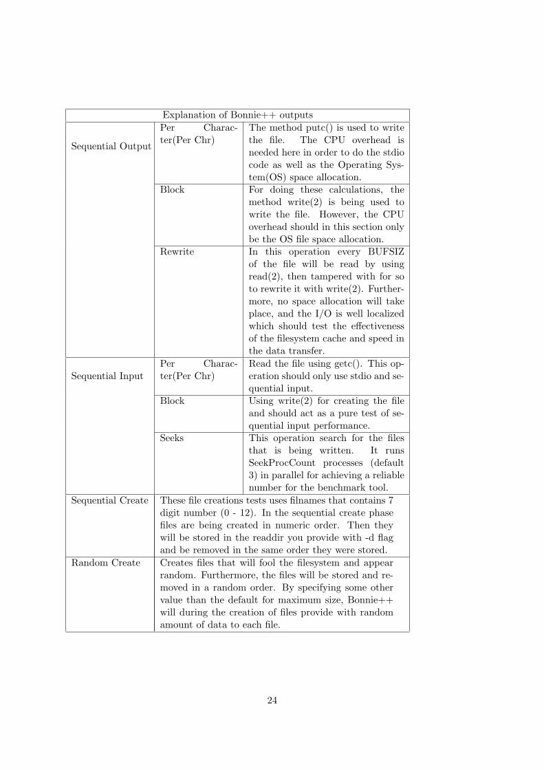
Explanation of Bonnie++ outputs
Sequential Output
Per Charac-ter(Per Chr)
The method putc() is used to writethe file. The CPU overhead isneeded here in order to do the stdiocode as well as the Operating Sys-tem(OS) space allocation.
Block For doing these calculations, themethod write(2) is being used towrite the file. However, the CPUoverhead should in this section onlybe the OS file space allocation.
Rewrite In this operation every BUFSIZof the file will be read by usingread(2), then tampered with for soto rewrite it with write(2). Further-more, no space allocation will takeplace, and the I/O is well localizedwhich should test the effectivenessof the filesystem cache and speed inthe data transfer.
Sequential InputPer Charac-ter(Per Chr)
Read the file using getc(). This op-eration should only use stdio and se-quential input.
Block Using write(2) for creating the fileand should act as a pure test of se-quential input performance.
Seeks This operation search for the filesthat is being written. It runsSeekProcCount processes (default3) in parallel for achieving a reliablenumber for the benchmark tool.
Sequential Create These file creations tests uses filnames that contains 7digit number (0 - 12). In the sequential create phasefiles are being created in numeric order. Then theywill be stored in the readdir you provide with -d flagand be removed in the same order they were stored.
Random Create Creates files that will fool the filesystem and appearrandom. Furthermore, the files will be stored and re-moved in a random order. By specifying some othervalue than the default for maximum size, Bonnie++will during the creation of files provide with randomamount of data to each file.
24

Chapter 3
Methodology
In the start of this project there were a few matters to consider. For measuring and collectingdata we decided to use the benchmarking tool bonnie++. Furthermore, we needed to analysethe data we received from these benchmarking tests. Since there was no tool available to per-form the necessary operations, one had to be made. The analys tool what was developed is aPerl script which will calculate average, median and variance on the data. That can be used ona later point to compare the different technologies.
3.1 Analysis Tool
In research where benchmark testing is being conducted, there is a necessity for analysis toolsthat can compress the outcome and make it representative for further studies. There are alreadya sourceforge project called bonnie-to-chart that performs different actions with the output datafrom bonnie++. Although there is a lot of interest for bonnie++ when it comes to analysisof the data and a tool like bonnie-to-chart is available, creating new framework tool seemedlike the best option. This way I could decide what type of data that is important and how theoutput would look like.
3.1.1 Input
The analysis tool is based upon a Perl script which handles a single output file at a time from abonnie++ session. It collects the data by using the file handler option in Perl and splits up allthe columns by using the split() feature. By reading the output files from bonnie++ sessionsyou will see a lot of data where ”+++” occurs. Every test will report two numbers, amountof work done and the percentage of CPU time taken when performing the test. The Author ofthis program implemented the ”+++” function to prevent wrong results[5]. Basically he thinksthat tests that completes in less than 500ms can not be calculated in an accurately way due torounding errors. Hence, displaying no result is better than displaying a wrong result. Therefore,when the scripts comes across a field that contains similar data it uses a regular expression toexchange the ”+++” to 0. Since the data, as mentioned above, is considered to be unreliablewhen the ”+++” symbols occur.
When done with the splitting up and sorting of the columns of data it goes into arrays foreasing the operation for doing descriptive statistics on the data. This make it possible for theuse of Perl modules. Math:NumberCruncher is the module that is being used for performing thestatistics on the data and simplify the operations for performing the calculations like Median,Mean, Average, Min/Max and Variation which will be described later on.
25

3.1.2 Usage
Describing the usage of this tool is simple. The users needs some basic understanding ofcomputers and know how operations are done in the Linux operating system. First of all abonnie++ session needs to be run in order to get data for the analysis tool to work with.Following line is an example of a session.
bonnie++ -d /tmp/ -x 100 -q -u root > /home/user/100x_nfs_1of3
The flag ”-d” indicates where the tests will be performed on the VM. Important thing toremember when deciding upon where the tests should be run is to check if you have enough freespace. Default value for the files will be 1 Gigabyte which was sufficient for these experiments.Although, if you would like to change the size you can use the ”-s” flag to change this. Thenumber of times the test is conducted is decided by the ”-x”. Without any value it will run asdefault only one time. For the analysis tool it would not matter whether it is 1 or 100, but forthe sake of having reliable data it would be best with 100 or more. The ”-q” is for quiet modewhich means that it will drop unnecessary output lines that is being produced while performingthese tests. The user performing these tests should be presented by the ”-u” flag. Files that willbe created and contain the data should be named in a fashion that it is easy to identify so thatthere will be no misunderstanding. Especially since there will be lot of tests if you scale up thenumber of VMs and bonnie++ is only able to write out which machine it is and not the typeof test that is taken. Furthermore, the name should contain the technology you are testing andwill be useful when several technologies are being tested at once. After a successful bonnie++session where you write the output to a file as shown above, it is then possible to use this fileas input for the analysis tool. Following line is an example of how to use the analysis tool.
bonperl.pl 100x_nfs_1of3 > /home/user/bonniedata/100x_nfs_1of3.tex
The file which is ”100x nfs 1of3” here will be analysed by the tool. Output from thisoperation will be printed out in a table format as well as a graph for each of the operations inlatex code. Reasons for this is to both save time and present the data in a manner so that itis easy to read. Although, first, it will be necessary to save the output to another file of yourchoosing. This file will then need to be compiled to a pdf file for making the data readable.Enter the folder where you put it and write the following command. It will depend on whetheryou have the latex packages installed for your operating system for a successful compilation.
pdflatex 100x_nfs_1of3.tex
26

3.2 Experimental Setup
Atlantis Nexus
Keeper Stargate
VirtualizationServers
Storage Servers
Switch
Figure 3.1: Figure of the lab setup
The lab setup of this project is seen on 3.1. These machines are members of an IBM Blad-server. Atlantis and Nexus will be acting as the virtualization servers, where we expand withmore vms if the tests requires more clients. All of the machines have bounded network cards,both with a 1GB capacity, making it a total of 2GB for each of the machine. The storage serverswill be Keeper and Stargate through the testing of the technologies and are meant to variatethe SAN software. Keeper will be the main machine for this, since most of the technologies onlyneed one machine as server. Hence, Stargate will be a backup when two machines are requiredfor setting up the specific SAN technology.
27

Bonnie++
Bonnie++
SAN ServerEXT 3
OS
OS
SAN SW
SAN SW
VFS
Virtual Machine
Dom0
Focus of Experiment
Constant
Service
Experimental Setup
VM filesystemsLVM/Files
Figure 3.2: experimental setup
Keeper has a variation of SAN software during these experimental tests as you can see on3.2. Dom0, that will be on the two machines atlantis and nexus which are connected to theSAN server, serves as an hypervisor for VMs. These machines also have SAN client software.Furthermore, in order for the VMs to act as clients for the SAN technology, a variation onthe SAN client software is also required. Since the VMs themselves can not interpret thatthey are connected to a SAN with current design. Moreover, the Dom0 has a constant Debiandistribution as a operating system that is used under every test of SAN technologies. The VMimage I use for these VMs only contains necessary file system with bonnie++ and does notcontain any network configuration. Each of these VMs has kernel(2.6.18-6-xen-686), runningext 3, and same operating system when they are booted up for testing.
3.2.1 Base tests
Comparative studies requires data that we can compare with, this is why these base tests aretaken. They give an indication on what is the optimal result you can get by running a testdirectly on the base of the system itself. By doing so we can then compare the results weget from these tests with the data from the actual experimental data, and then determine itsstrengths or weaknesses.
Base tests that are to be run during this project:
• Keeper which is the SAN server
• Virtualization server with no VMs up
28

• Virtualization server with one VM up
• Virtualization server with ISCSI installation
• Virtualization server with NFS installation
• Virtualization server with DRBD installation
• Virtualization server with AoE installation
• Virtualization server with Pvfs installation
3.2.2 non-Base tests
These tests are the actual experimental data. Where the variation of the SAN technology isin focus and the scaling of clients is the main process for identifying the best one based on thecomparison of the data.
3.3 Output
Under these experimental benchmark tests there is an expectation that a random SAN technol-ogy test should have the same performance as a base test on keeper or worse. Hence, we canthen expect that a virtual machine placed on top with a random SAN technology should per-form just as well or worse as the base test. As mentioned earlier an output file should be namedaccordingly to the test that is taken. In doing so scaling of the VMs will be more systematicand thorough. Each technology will require a considerable increase of clients in each scenariowhich will generate a lot of files. Keeping a system is then crucial when compiling these filesto an appropriate format, especially when using pdflatex on the generated latex tables that aregenerated from the analyse tool.
3.4 Analysis
In this section the different measurements will be listed and explained in detail. It will alsoexplain what kind of meaning they have for the investigation and how it helps in identifyingthe best SAN technology.
• MedianMedian will be one of the two ways to find the average. It does it by arranging the valuesin order and selecting the one number in the middle. However, if the values from a seriesof tests or a sample is even, the median will be the mean of the two middle numbers.
• MeanMean is the second way to find the average and will be the sum of these measurementsthat is taken during the test of each technology divided by the amount of measurementstaken.
• MinFinding the minimum value that is recorded during a test could determine how low theperformance of the technology went during an experiment. Hence, be an important factorwhen deciding what the best technology is, and how it adds up with variation number.
29

• MaxMaximum value determines the highest performance score of the technology which willalongside the minimum value help us gain the whole picture of how the technology works.Furthermore, the maximum and minimum of the measured results will give a performancepoint of view were for the given technology.
• VariationVariation is of great importance for finding the most stable SAN technology. Seeing asthe greater the number, the greater the performance of the technology variates whichmakes it difficult to rely on. System administrators wants a reliable technology that hasthe same performance most of the time and not take chances on one that might performmuch better in a certain amount of time. Although, it would be better for me if I had amathematical distribution as well in order to fully understand the variation results.
30

Chapter 4
Results
The results from these base tests is what can be called the optimal performance from the oper-ations of the benchmark tool bonnie++. These results will be an important factor in decidingthe best SAN technology when comparing scores.
4.1 Explanation of output in tables
In the first block session we can see the name of the machine and what file size this bonnie++session used to perform the different operations with. File size can be changed but the de-fault value is used for all of the bonnie++ sessions. Next block contains putc which producesoutput and writes in two modes, by character and by block. The output results from putcand putc block are measured in kilobytes per second(KB/s) while putc cpu and put block cpucontains the percentage of the cpu used during these operations.
After the writing process, bonnie++ will do a rewrite operation of the current files whichwill also be measured in KB/s. Then we reach the reading section which is organized by thegetc and getc block operations. Both of these operations are also measured in KB/s while thegetc cpu and get block cpu are the percentage of cpu used during these operations. Measuringseeks is the next section where seeks are files found per second and seeks cpu is the percentageused during the search for files. The amount of files is mentioned in num files, if you want youcan specify yourself how many files that should be in this test and also how the size should bedivided between them with the bonnie++ flags. Although, 16 files is the default value and wasused when testing all of the SAN technologies.
When it comes to the sequential operations, only seq create and seq create cpu will beinteresting in terms of data. The other operations will finish up to quickly to be a reliable resultand not worth mentioning. However, for the random operations, only ran stat and ran stat cpuwill be unreliable data. ran create will show how many files that are created in a random orderper second while the ran create cpu will show the percentage of cpu usage during this time.ran del show how many files that are deleted in a random order per second.
4.2 Keeper basetest
Results from the base test of keeper with no SAN technologies installed. It runs a basic Debianinstallation with a few alterations from the ABC startsidens security systems. Although, this
31

should not affect the outcome in any way, when it comes to disk activity during these bench-marking tests.
Name Mean Median (Mean -Median)
Variance Min Max Range
name 0 0 0 nan keeper keeper 0file size 7 7 0 nan 7G 7G 0putc 45871.808 45853 18.808 59109.751 45403 46607 1204putc cpu 95.515 95 0.515 0.290 95 97 2put block 70315.303 70885 569.697 2073288.373 65950 72880 6930put block cpu 24.333 24 0.333 0.424 23 25 2rewrite 29713.081 30009 295.919 318502.943 28480 30459 1979rewrite cpu 7 7 0 nan 7 7 0getc 49877.535 50453 575.465 1830404.491 45300 51507 6207getc cpu 91.141 92 0.859 5.637 83 94 11get block 72161.899 72627 465.101 1819859.364 65732 73967 8235get block cpu 5.020 5 0.020 0.020 5 6 1seeks 537.737 546.300 8.563 2953.941 344.6 617.0 272.4seeks cpu 0.354 0 0.354 0.229 0 1 1num files 16 16 0 nan 16 16 0seq create 3658.535 3658 0.535 1816.835 3464 3721 257seq create cpu 97.929 98 0.071 1.217 93 99 6seq stat 0 0 0 nan 0 0 0seq cpu 0 0 0 nan 0 0 0seq del 0 0 0 nan 0 0 0seq del cpu 0 0 0 nan 0 0 0ran create 3746.556 3747 0.444 1354.186 3592 3795 203ran create cpu 98.152 98 0.152 0.977 94 99 5ran stat 0 0 0 nan 0 0 0ran stat cpu 0 0 0 nan 0 0 0ran del 11893.172 12085 191.828 115392.162 11091 12277 1186
Table 4.1: Table of keeper basetest
Overall results
The operation putc shows less to no difference between its mean and median value by only 18KB/s. Seeing as this is the base test which should be the best optimal result that we are goingto compare with, 45 MB/s is not such a bad performance. By a quick overview we can also seethat putc block performs better than putc and uses less cpu load to accomplish that. Although,a bit higher difference we can see but not really alarming.
The rewrite operation is lowered to 30 MB/s which is still good performance if you thinkabout the buffering refreshing itself all the time it is running. Furthermore, reading operationsscore slightly higher than writing. The getc with 50 MB/s and get block with 72 MB/s aregood results. Seeks has also quite similar numbers in mean and median, 537 to 546 files persecond.
32
Moreover, the seq create creates 3658 files in an average per second, and the cpu load ishigh which also is normal. The other functions does not show which is normal, since they finishup to fast for it to be any reliable data according to the author of the program. ran create getsa bit higher performance on mean and median compared to the seq create. It also uses a lotof cpu during this operation. Last operation, the ran del, shows good performance by deleting12000 files per second.
Descriptive statistics
putc has a a range of 1,2 MB/s between the max and min value which indicates a stable workrate. Furthermore, this could also make it easier to predict the time span of how long it wouldtake to finish writing over files for instance when it comes to backup. putc block gets higherspeed and has much higher max than min. Seeing as mean and median is around 70 MB/s, themin value seems to be very poor performance for this operation and it gives a greater rangewith 6,9 MB/s which indicates much more unstable results. Moreover, the percentage of cpuused between putc and putc cpu is significant, reasons for this could be that the cache is morepresent in the putc operation.
Rewrite operations goes around 30 MB/s which is around 15 MB/s slower than putc per-formed, this could be that is has to take into account the order of the files when it rewrites,making it drop some performance on the way. The reading operations performs slightly higherthan the writing. Both getc and get block have a larger range between max and min than thein the writing operations. Furthermore, if we look at get block we can see that average perfor-mance measured by mean and median are close to the max value, which makes it interesting tosee if it was a slight irregularity or if it actually will be noticeable in the other experiments.
seq create performs a bit lower than the ran create, where seq create has a total of 3658files per second while ran create has 3746 files per second. Both seems to be working at a stablerate as well according to the range of the min and max values. Same with the cpu usage duringthese two operations with a 98 percent usage. The deletion of the files goes at a much higherperformance, ran del has an average of 12000 files deleted per second. Although, it has a largerrange between the max and min values which tells us that it is not as stable as during thecreation of the files.
33

Graphs of interest
Figure 4.1: keeper put block
As we can see from figure 4.1 the mean values of put block seems to match the averagemeasurements for this operation. With most hits in the area between 69 MB/s to 71 MB/swhich corresponds well with the value of 70 MB/s in the mean. From figure 4.2 we can clearly
Figure 4.2: keeper get block
see that the mean value of 72 MB/s is accurate according to where the most hits were recorded.Seeing as there is close to 60 hits at 72 MB/s for the get block operation. By looking at theseeks operations for keeper in 4.3 we can see that the mean value of 537 is valid according tothe hits recorded. The graph shows that most of the hits were around 550 files per second.
34

Figure 4.3: keeper seeks
Summary
Looking through the results of the benchmark test, some results were more interesting than theothers. Reading performs higher than writing, while rewriting goes even lower. In both of theseoperations we can also see how the difference between the by char and block transfer is high.When performing the put block and get block the cpu resources used are low and they use mostof the time to wait for the hard drive during their operations. In the reading operations themaximum values are closer to the median and mean values than the minimum value that couldbe explain by some slight irregularities during the benchmark test.
4.3 Nexus basetest
This section will display the results measured from the benchmark test run on nexus, which isone of the virtualization servers, with no VMs up and running.
Name Mean Median (Mean -Median)
Variance Min Max Range
putc 42277.101 42338 60.899 124824.454 41292 42961 1669putc cpu 94.990 95 0.010 0.677 93 96 3put block 66632.576 66897 264.424 2759297.557 62611 69596 6985put block cpu 32.263 32 0.263 0.658 30 34 4rewrite 28845.606 29132 286.394 428861.794 27614 29599 1985rewrite cpu 3 3 0 nan 3 3 0getc 47166.556 47548 381.444 2035148.449 41837 49144 7307getc cpu 84.909 86 1.091 7.941 75 88 13get block 70311.222 70641 329.778 939812.112 66732 71550 4818get block cpu 0 0 0 nan 0 0 0seeks 486.417 497.200 10.783 3614.723 321.6 595.2 273.6seeks cpu 0 0 0 nan 0 0 0
Table 4.2: Table of nexus basetest
35

Overall Results
In the writing section we see a good performance on the putc operation with 42 MB/s in meanand median. It also has a min value of 41 MB/s and close to 43 MB/s in max. put blockperformance is acceptable, with 66 MB/s in mean and median, and a min value of 62 MB/sand max value of 69 MB/s. rewrite does more than half of the putc operation with a 28 MB/sin mean and 29 MB/s in median. The min and max values have a bit more gap between thanputc with 27 MB/s and 29 MB/s.
The reading operations performs better than writing. getc has a mean and median value of47 MB/s and get block has a mean and median value of 70 MB/s. Looking at their min andmax values, we can see that getc has 41 MB/s min and 49 MB/s max while get block has 66MB/s min and 71 MB/s max.
The seek operation has a good performance with 486 files per second in mean and 497 filesper second in median. It also has a min value of 321 files per second and a max value of 595files per second. The rest of the operations during this benchmark were to fast to measure anycredible data.
Descriptive statistics
During this benchmark test reading operations have performed better than writing. Although,getc performed better if we look at the mean and compare it with putc, we can see that getc hasa much wider range between its min and max values. This suggest that this operations workrate is unstable. However, for the put block and get block the situation has changed. Seeinghow get block both performs better if we look at mean and median, and has a lower range with4,8 MB/s versus put block with 6,9 MB/s.
The rewrite operation only has half of the performance putc has in mean and median, butseems to be waiting a lot for the disk to complete because of a very low cpu usage of 3 percent.Irregularities of some kind could be causing this like for instance caching. seeks performanceswell but has a wide range with 273 files per second, which would strongly suggest an unstablework rhythm.
Graphs of interest
These are the graphs of operations that are most interesting when it comes to these benchmarktests.
Figure 4.4 show that most of the measured results are resided in the area between 64 MB/sto 69 MB/s which seems to in balance with the calculated mean value in table 4.3. Same goesfor the data we see in figure 4.5 with most of the measured results in between 69 to 71 MB/sand a value of 70 MB/s in mean in table 4.3.
36

Figure 4.4: Nexus novm putblock
Figure 4.5: Nexus novm getblock
Figure 4.6: Nexus novm seeks
37

In figure 4.6 we can see that most of the data are measured in the area between 45 to 55files per second. It makes the number of 486 files per second in mean valid from table 4.3.
Summary
In this base test we have seen how reading operations perform better overall. However, bothwriting and reading have some instability if we look at their ranges. This also applies for seeksthat has close to half of the max value in range with 273 files per second. Furthermore, thecreation and deletion tests from this benchmark operated at such a fast rate that there couldnot be measured any valid data.
38

4.4 Nexus with one VM
This data set contains the measurements collected from the test performed locally on the vir-tualization server Nexus with one VM running.
Name Mean Median (Mean -Median)
Variance Min Max Range
putc 48393.960 48634 240.040 363248.402 46306 48872 2566putc cpu 96.869 97 0.131 0.114 96 97 1put block 278673.899 281531 2857.101 213690989.465 233369 307593 74224put block cpu 76.283 77 0.717 5.031 71 81 10rewrite 77605.869 77633 27.131 25588185.508 67363 91479 24116rewrite cpu 12.444 12 0.444 1.116 10 15 5getc 51685.818 51909 223.182 482574.694 49109 52450 3341getc cpu 93.758 94 0.242 0.992 91 95 4get block 447152.869 450941 3788.131 559635801.952 355290 471783 116493get block cpu 7.616 7 0.616 10.014 2 19 17seeks 0 0 0 nan 0 0 0seeks cpu 0 0 0 nan 0 0 0seq create 4136.919 4147 10.081 1011.973 4002 4160 158seq create cpu 99.313 99 0.313 0.215 99 100 1seq stat 0 0 0 nan 0 0 0seq stat cpu 0 0 0 nan 0 0 0seq del 0 0 0 nan 0 0 0seq del cpu 0 0 0 nan 0 0 0ran create 4276.253 4289 12.747 1487.441 4107 4307 200ran create cpu 99.091 99 0.091 0.083 99 100 1ran stat 0 0 0 nan 0 0 0ran stat cpu 0 0 0 nan 0 0 0ran del 16213.616 16237 23.384 58919.166 15187 17719 2532
Table 4.3: Table from Nexus onevm
Overall Results
In the writing operations we can see that the putc has a good performance of 48 MB/s bylooking at the mean and median values. These numbers seems to be close up to the max valueof this operation. put block has a very good performance with a mean of 278 MB/s and medianof 281 MB/s, and a max performance of 307 MB/s. Cpu usage of the two operations are quitehigh, 96 percent with putc and 76 percent with put block. The rewrite operation has 77 MB/sin mean and median, and a min value of 67 MB/s and a max value of 91 MB/s. Its cpu usageis lower compared to the writing operations putc and put block with only 12 percent usage.
getc and get block in the reading section also performs well on this benchmark test. getchas a measured and calculated value of 51 MB/s in mean and median while get block gets 447MB/s in mean and 450MB/s in median. This operation scores very high at these tests whichwe can see even more clearly from the min and max values, seeing as its min value is 355 MB/swhich is even higher than the max value of put block. Furthermore, the max value for get block
39

is 471 MB/s which is over two times as much as the min value of put block.
In the last two sections we can see similar results for the seq create and the ran create.seq create has a value of 4136 files per second while ran create has 4147 files per second. Theyboth have the same amount of cpu usage during these operations with a 99 percent usage. Lastis the ran del operation which has a measured mean and median value of 16 MB/s.
Descriptive Statistics
The two first sections have some very good results from these tests but unstable. If we lookat the put block values we can see a big difference in the mean and median values as well asa wide range. A range of 74 MB/s would suggest an unreliable rhythm of its operation. Thebig difference of the mean and median only strengthens this assumption. Same goes for therewrite and get block operation, rewrite with 24 MB/s and get block with 116 MB/s wide range.
However, in the last two sections we can see a more stable work rate and good results. Bothseq create and ran create having a less to no difference between the mean and median. Only10 KB/s for seq create and 12 KB/s for ran create. ran del as well with a 23 KB/s difference,although, it shows a slight instability if we look at the range of its min and max values.
40
Graphs of interest
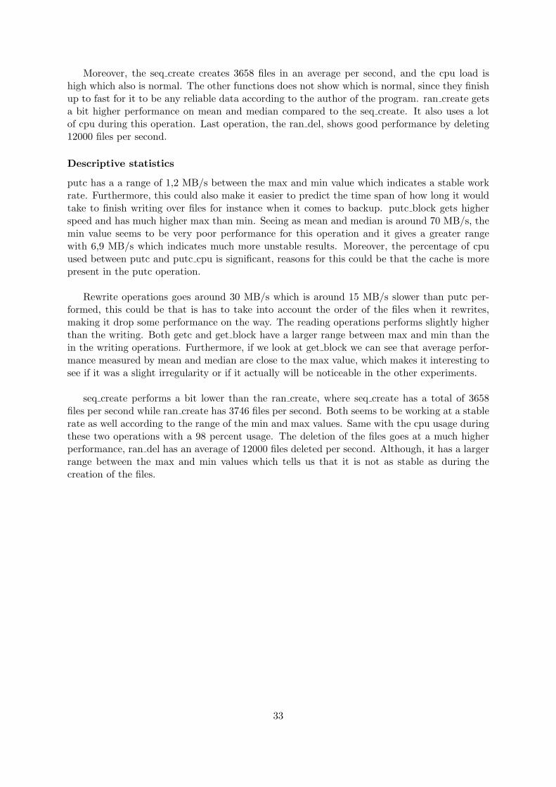
The seek operation did not contain any credible data during this test. However, the graphs forput block and get block have valid data and will be presented. Figure 4.7 shows that the mean
Figure 4.7: Nexus onevm put block
value calculated for the put block operation seems to be coordinating well with the values inthe graph. Seeing as the area between 260 MB/s to 290 MB/s has the most hits.
Figure 4.8: nexus onevm get block
Furthermore, we can see from figure 4.8 that the most hits are around the area between 440MB/s and 470 MB/s. Hence, making the calculated mean value credible and giving a correctpicture of how the performance was during the process.
Summary
This benchmark test of the virtual server running with one VM shows good performance, al-though, it has some unstable results in the writing and reading section. Especially the put block,rewrite and get block were the ones that seemed to be the most affected by this. However, the
41

rest of the results of this benchmark test shows good and stable results with no alarming num-bers.
4.5 Iscsi basetest
These are the results for the iscsi base test. The virtualization server runs with one VM and theserver itself has a basic iscsi configuration which establishes contact with the iSCSI technologyon the SAN server.
Name Mean Median (Mean -Median)
Variance Min Max Range
putc 42653.101 42781 127.899 738863.323 37996 44117 6121putc cpu 84.848 85 0.152 2.553 75 88 13put block 45046.192 45216 169.808 482467.145 40918 46096 5178put block cpu 6.697 7 0.303 0.312 6 8 2rewrite 11346.717 11235 111.717 77779.880 10858 12216 1358rewrite cpu 0 0 0 nan 0 0 0getc 14439.909 14465 25.091 76518.891 13491 15209 1718getc cpu 6.596 7 0.404 0.483 4 8 4get block 18294.232 18291 3.232 132275.875 17223 19437 2214get block cpu 0 0 0 nan 0 0 0seeks 478.597 477.800 0.797 266.913 404.3 570.1 165.8seeks cpu 0 0 0 nan 0 0 0seq create 4041.636 4037 4.636 3856.231 3838 4212 374seq create cpu 96.929 97 0.071 1.379 94 101 7seq stat 0 0 0 nan 0 0 0seq stat cpu 0 0 0 nan 0 0 0seq del 0 0 0 nan 0 0 0seq del cpu 0 0 0 nan 0 0 0ran create 4242.646 4278 35.354 5385.319 3884 4469 585ran create cpu 98.525 99 0.475 1.987 96 104 8ran stat 0 0 0 nan 0 0 0ran stat cpu 0 0 0 nan 0 0 0ran del 15243.495 14859 384.495 685322.775 13981 16433 2452
Table 4.4: Table of iscsi basetest
Overall Results
In the writing section one can see that both putc and putc block have a very small differencebetween their mean and median. We can also see that the cpu usage is very low on the put blockcompared to the putc. Rewriting seems perform at a much lower rate than putc and put blockwith a difference of 30 MB/s or more. Although, the speed of the operation is very low it hasa stable work rate looking at the max and min values.
Reading section of this benchmark test operates on a much lower performance than whenit comes to writing. Results from mean and median show 14 MB/s which is under half of whatwriting section performs The cpu performance of the getc and getc block are very low, especially
42

the getc block which does not report any number even. Seeks seems to be working fine with anumber of 478 files found per second. In seq create 4000 files is created per second from whatwe can see in the mean and media which is a good performance. Same goes for the ran createwith 4200 files and ran del with 15000 files created per second. All of the creation operationswork with little difference in both average and the range between the max and min values.
Descriptive statistics
Iscsi performance varies a lot during the writing operations putc and put block. If we look atthe max and min values they get, we see the range being large. This could indicate that theiscsi performs on an unstable rate but by looking at the mean and median, it would be morereasonable to assume that some irregularities could have caused this during the measurements.Rewriting has a very low performance as we can see compared to the putc and putc block pro-cesses. Although, is shows a more stable work rate if we look at the range between max andmin. putc and put block with 6 MB/s and 5 MB/s while rewrite performs with a range of 1,3MB/s.
Reading operations also performs at a more stable rate than the putc and put block. getcand get block have ranges of 1,7 MB/s and 2,2 MB/s. Furthermore, getc and get block have amuch lower performance on the mean and median with 14 MB/s and 18 MB/s, that is reallylow if we think about what I/O measurement would look like for a normal hard drive. Seeksoperations does good performance with 478 hits per second and has less to no difference withits mean and median values. Same goes for the max and min values with a range of 374 filesper second.
In the last two sections where files are created and deleted, both seq create and ran createhave similar results in mean and median. The difference on their mean and median is very smalland not alarming. Furthermore, we can also see that the range indicates a stable performancebased on their max and min values. Although, ran del has a much higher performance inthe mean and median, the operation gains a bit more instability Seeing as the number in thedifference and range of its operations rises.
43

Graphs of interest
Figure 4.9: iscsi putblock
The graph in figure 4.9 shows good argumentation for the calculated mean value from table4.5, seeing as most of the measurements recorded were found around 43 and 46 MB/s. Figure
Figure 4.10: iscsi getblock
4.10 shows that most of the measured values are found in the area from 16,5 MB/s to 19 MB/s.This makes the mean value from table 4.5 valid which has a value of 18 MB/s. By studying thegraphs in figure 4.11 we see that most of the measurements were recorded in the area between430 to 460 files per second. This suggest that the mean value from table 4.5 is affected byunstable work rate during the benchmark test.
44

Figure 4.11: iscsi seeks
Summary
One thing in particular that really is abnormal in these measurements is the difference betweenthe writing and reading operations. We can assume that there should be a slight differencewhen it comes to reading and writing, although, the difference we see here is really interesting.The number of getc is performing on less than half of what putc manages to produce per secondaccording to the mean and median values. Normally, the reading operations usually performon the same work rate as the writing operations do or better. Furthermore, we can see somelower cpu usage from some of the operations which indicates that they are waiting for the harddrive to finish up before they can start on their next operation.
45

4.6 Iscsi 3of3 test
These are the results for iscsi where three VMs are run upon Atlantis. Atlantis has iscsi clientsoftware installed and is connected to keeper that runs as the iscsi server with the proper soft-ware. This table is the representative data from all the three VMs that were running bonnie++and gives an indication on how VMs are affected when more than one are operating on theshared iscsi device.
Name Mean Median (Mean -Median)
Variance Min Max Range
putc 16258.444 16021 237.444 11392432.166 12011 28651 16640putc cpu 34.626 35 0.374 42.820 25 59 34put block 15246.657 13532 1714.657 8762264.286 12583 21367 8784put block cpu 2.323 2 0.323 0.239 2 4 2rewrite 4440.919 4329 111.919 172536.923 3675 5821 2146rewrite cpu 0 0 0 nan 0 0 0getc 7730.374 7994 263.626 599217.668 5974 11023 5049getc cpu 3.283 3 0.283 0.607 2 5 3get block 8996.253 9353 356.747 2426084.492 6444 18603 12159get block cpu 0 0 0 nan 0 0 0seeks 231.807 235 3.193 7046.147 85.5 482.3 396.8seeks cpu 0 0 0 nan 0 0 0num files 16 16 0 nan 16 16 0seq create 3648.152 3816 167.848 168373.785 2434 4102 1668seq create cpu 95.172 96 0.828 7.496 86 99 13seq stat 0 0 0 nan 0 0 0seq stat cpu 0 0 0 nan 0 0 0seq del 0 0 0 nan 0 0 0seq del cpu 0 0 0 nan 0 0 0ran create 3683.465 3866 182.535 221465.461 2476 4303 1827ran create cpu 95.556 96 0.444 7.277 84 100 16ran stat 0 0 0 nan 0 0 0ran stat cpu 0 0 0 nan 0 0 0ran del 13978.010 14799 820.990 4517906.879 8749 16253 7504
Table 4.5: Table of iscsi 3of3 test
Overall Results
By a quick overview of the writing section we can see a greater gap between the put block anputc when it comes to the difference of mean and median. Furthermore, we can see that it isthe other way around in the range between max and min for these two operations. putc witha 16 MB/s range and put block with a 8 MB/s. Both of these operations have a very low cpuusage, especially put block with only 2 percent. Rewriting has lower performance as we can seeof the mean and median but has a smaller range between its max and min with 2 MB/s. Thereading section also has a large range in the getc and get block operations between the maxand min values. getc has a 5 MB/s while get block has 12 MB/s. The Seeks operation appearsto get a low performance by looking at the mean and median.
46

seq create has good performance if we look at the mean and median values. Although, itdoes not have the range of the other operations, it is still considerable if we look at the max andmin values. Same goes for the ran create, shows good performance in the mean and medianvalues but also has a big range if we look at the max and min values. Cpu usage of theseoperations is high which is to be expected with 95 to 96 percent usage. ran del performs 13,9MB/s in mean and 14,7 MB/s in median which leads to a bigger difference if we compare tothe values for seq create and ran create. Moreover, the range for ran del is high compared tothe range for seq create and ran create.
Descriptive statistics
Both writing and reading operations for the iscsi benchmark test are showing unstable workingrate if we look upon the max and min values. putc has a min value of 12 MB/s and a maxvalue of 28 MB/s which ends up in a range of 16 MB/s. This strongly suggest that it worksin an unstable manner. Especially if we compare the mean and median values and see howthe max value is so much higher, assumptions could be made to describe it as unreliable aswell. Although, the range is half on the put block operation, the difference in the mean andmedian values is 1,7 MB/s. A very high number compared to the putc operation which stronglyindicates an unreliable work rate. rewrite has very low performance as we already covered inthe last section, but the range of the max and min values shows a more stable work rate forthis operation.
Furthermore, both getc and get block have a shorter range compared to putc and put block,they are still too high to be seen as reliable. Although, the unstable results shown in range, wecan see that the difference between the mean and median are acceptable with only 0,26 MB/sfor getc and 0,35 MB/s for get block. In the searching section looking at the seek operationwe see a very low min value of 85,5 files per second. The range is also very high compared thenumber we have in max with a range of 396 files per second and a max value of 482 files persecond. This low min value could be explained by some irregularities during these benchmarktests like for instance the cache of the cpu on the VM server acting up.
In the section where creating files are being measured we can see from both seq create andran create a stable work rate. seq create has a a difference of 167 files per second which indicatesa reliable work rate and a range of 1,6 MB/s that is acceptable compared to the values we seefrom the writing and reading operations. Lastly we see the ran del performs at a much higherrate than both seq create and ran create by looking at the mean and median values of theseoperations. Moreover, the difference is higher but not really affecting the stability as much asthe range. The range between its max and min is are much higher than the max and min ofseq create and ran create, indicating an unstable rhythm in its working rate.
47

Graphs of interest
Figure 4.12: iscsi 3of3 putbl
Figure 4.12 shows the measurements recorded for the put block operation. As we can seethe results are widely spread and there are many counts both at the start and at the end. Thiscould indicate that the mean value from table 4.6 is unbalanced based on the data we see inthe graph. However, figure 4.13 shows that the get block operation data from the table 4.6 and
Figure 4.13: iscsi 3of3 getblock
the graph works in harmony.
48

Figure 4.14: iscsi 3of3 seeks
Same situation can be seen in figure 4.14 since most of the measurements are recordedbetween 100 to 350 files per second and the mean value for the seek operation in table 4.6 is on230 files per second.
Summary
By looking through what we have observed, one thing in particular should be mentioned. Thedifference in the performance between the writing and reading section was really the mostinteresting. Seeing as the reading performance is measured to be half of what the performancein the writing got but still they are operating at the same unstable work rate. Despite of thebad performance in these two sections the ways of testing creating and deleting files scored high.Both the difference and the range were at an acceptable number and indicating a more stablework rate.
49

4.7 NFS basetest
This table shows the results from a NFS base test that was conducted on the virtualizationserver Atlantis It was run without any VMs and Atlantis used the benchmark tool directly onthe environment shared by NFS.
Name Mean Median (Mean -Median)
Variance Min Max Range
putc 28534.444 28419 115.444 611578.954 27089 31697 4608putc cpu 60.212 60 0.212 3.238 57 67 10put block 27021.515 26818 203.515 1616586.290 24888 30831 5943put block cpu 9.525 9 0.525 0.330 9 12 3rewrite 13358.869 13337 21.869 47389.791 12861 13942 1081rewrite cpu 2.212 2 0.212 0.167 2 3 1getc 23866.505 23721 145.505 647568.452 22146 26212 4066getc cpu 44.576 45 0.424 24.608 33 55 22get block 25155.343 25202 46.657 334903.781 23635 26436 2801get block cpu 5.475 6 0.525 0.977 4 8 4seeks 1049.258 1068.800 19.542 6178.578 615.0 1177.2 562.2seeks cpu 1.788 1 0.788 8.329 0 13 13seq create 38.697 39 0.303 0.433 38 40 2seq create cpu 0 0 0 nan 0 0 0seq stat 4472.424 3714 758.424 1549846.850 3600 6756 3156seq stat cpu 1.333 1 0.333 2.485 0 9 9seq del 77.657 78 0.343 2.407 74 79 5seq del cpu 0 0 0 nan 0 0 0ran create 39.101 39 0.101 0.273 37 40 3ran create cpu 0 0 0 nan 0 0 0ran stat 4939.737 4005 934.737 2523425.547 3916 7943 4027ran stat cpu 0.465 0 0.465 1.239 0 9 9ran del 78.404 79 0.596 0.726 77 79 2
Table 4.6: Table of NFS basetest
Overall Results
In the writing section of the NFS base test we can see that there is a very small differencebetween the mean and median of putc with a 115 KB/s. However, its range between the minand max shows a larger difference with a number of 4,6 MB/s. put block seems also to have thesame phenomena with a difference for the mean and median of 203 KB/s and a range betweenthe min and max values of 5,9 MB/s. We can see that the cpu usage is much lower for theput block with a 9 percent usage compared to the putc operation that uses 60 percent duringits run.
rewrite operation performs at 13 MB/s which is a bit under half of the performance thewriting section produces during the benchmark tests. Furthermore, the difference of its meanand median values is only 21 KB/s. Moreover, the range of the min and max values is 1 MB/s.Both of these values are much smaller than the writing sections values. Same goes for the cpu
50

usage as well with only 2 percent usage as we can see from looking at the mean and median values
The reading section has similar results as in the writing section. getc has 23 MB/s whileget block has 25 MB/s in mean and median. They have the same phenomena as in the readingsection with little difference between the mean and median and bigger range when it comes tothe max and min values. We can also see that the cpu usage for the getc and get block is lowerwith 44 percent and 5 percent usage. seeks seems to be performing quite well with a strongmean of 1049 files and a median of 1068 files per second. Although, the min value 615 files persecond is only half of the maximum number of 1177 files per second.
By looking at the file operations like creating and deleting we clearly see bad performancefor being I/O benchmark tests. seq create produces only between 38 to 39 files per secondaccording to the mean and median values. The performance of this NFS base test is so lowthat we can get a number from the seq stat. This operation reads through the file and sendsback the information about it like for instance permissions. In the mean we see that is stats4472 files per second while in median it is 3714 files per second. This gives a higher differencethan the previous operations for this base test. seq del also has a low performance by lookingat the mean value of 77 files per second and median of 78 files per second. The range of theseoperations is very low and seems to be stable.
Next section which creates files in a different order seems also to perform low. ran createhas a mean and median at 39 files per second which corresponds well with the min and maxvalues. ran stat performs a bit higher compared to the seq stat but this is also goes for thedifference of its mean and median values. Both seq stat and ran stat produces a very high rangeand seem to have had problems during the benchmark test. ran del performs on the same levelas seq del.
Descriptive statistics
Writing and reading section have similar results produced from this benchmark test. There isless to no difference in the mean and median values of the putc,put block,getc and get blockoperations. However, we can see that putc and put block have a larger range than the getc andget block, indicating a much more unstable work rate when it comes to writing. Moreover, therewriting operation performs with a lower mean and median but at a more stable work ratewith a range of 1 MB/s.
seeks is performing very well if we look at the mean and median values, up to 1000 files persecond. Although, if we look closer at the min and max values, 615 and 1177 files per second,there is a wide range between them. Seeing as the mean and median values are much closer tothe max value than the min value, we could assume that some irregularities during its operationoccurred, causing bad results.
In the next sections we see operations with poor performance operating at stable work rate.seq stat and ran stat stands out as the more unstable ones. Especially if we look at their maxand min values. They both have quite wide ranges, seq stat with 3156 files per second andran stat with 4027 files per second. The max value from both of them is also twice as big as themean and median values, which strongly suggests a very unstable and unreliable work rate forthese operations. Furthermore, seq create, ran create and ran del have low performance but avery stable work rate with a range of 2 to 5 files per second.
51

Graphs of interest
Figure 4.15: NFS base putblock
Figure 4.15 shows that the mean value from table 4.7 for the put block operation seems tobe accurate according to the graphs. In figure 4.16 we see that most of the values are resided
Figure 4.16: NFS base getblock
in the area between 22,5 MB/s to 26,5 MB/s. This validates the mean value of 25 MB/s fromtable 4.7
52

Figure 4.17: NFS base seeks
From figure 4.17 we can see that the measurements recorded are heavily populated in thearea between 900 to 1150 files per second. These values corresponds well with the mean valuefrom table 4.7.
Summary
The overall results for this base test shows a very poor performance. Especially in the twosections that handles and tests the creation and deletion of files. seq create and ran creategoing as low as 38 to 39 files per second when we look at their mean and median values. Thisalso affects the outcome of the seq stat and ran stat that usually performs to fast to get a validmeasurement, because of the slow performance we can do some descriptive statistics of the datacoming from those operations as well. Seeks is the only operation under this base test thatperforms well from what we have seen earlier.
53

4.8 NFS 3of3 test
From this table of data we can see the results from three VMs running a bonnie++ benchmarktest on one of the virtualization servers, in this case Atlantis, which is connected to a sharedand mounted folder.
Name Mean Median (Mean -Median)
Variance Min Max Range
putc 25321.253 28261 2939.747 97671354.229 5540 40616 35076putc cpu 73.343 94 20.657 827.700 15 97 82put block 104609.697 111786 7176.303 6174875548.393 5495 289875 284380put block cpu 35.444 38 2.556 715.863 1 85 84rewrite 53472.293 51444 2028.293 1705559591.035 4035 180698 176663rewrite cpu 9.293 8 1.293 76.268 0 33 33getc 21595.960 24070 2474.040 139606583.554 106 47859 47753getc cpu 54.051 58 3.949 935.725 0 95 95get block 141666.374 143731 2064.626 13727079249.163 6287 430634 424347get block cpu 4.980 2 2.980 37.111 0 23 23seeks 3005.201 306.200 2699.001 23392375.841 0 16365.1 16365.1seeks cpu 2 0 2 17.455 0 17 17seq create 2715.535 2929 213.465 1122266.734 355 4151 3796seq create cpu 84 99 15 898.929 9 102 93seq stat 0 0 0 nan 0 0 0seq stat cpu 0 0 0 nan 0 0 0seq del 35.293 0 35.293 122067.904 0 3494 3494seq del cpu 0.020 0 0.020 0.040 0 2 2ran create 3010.030 3037 26.970 830162.595 342 4280 3938ran create cpu 90.667 99 8.333 512.303 10 100 90ran stat 0 0 0 nan 0 0 0ran stat cpu 0 0 0 nan 0 0 0ran del 11903.657 12049 145.343 14317081.256 680 16409 15729
Table 4.7: Table of NFS 3of3 test
Overall Results
By a quick view in the writing section we can see that the putc performs much lower thanput block, putc has a mean of 25 MB/s and a median of 28 MB/s while put block has 104MB/s and 117 MB/s. Both of the operations have a high difference between the mean and me-dian, same conditions can be stated for the ranges. putc has a range of 35 MB/s and put blockwith a 284 MB/s which seems to be very high. rewrite has twice the performance in mean with53 MB/s and almost the same in median which looks a bit suspicious compared to what wehave seen before. Its range is also very high with a number of 176 MB/s.
In the reading section we have the same phenomena where getc operates with a mean valueof 21 MB/s and median of 24 MB/s while get block has the mean value of 141 MB/s and 143MB/s in median. Furthermore, we can see wide ranges according to their min and max valuesas well. getc with a 47 MB/s and get block with a very high range of 424 MB/s. Moreover,
54

the seeks operation has a very big gap between its mean and median, seeing as its mean is 3005files per second and median only 306 files per second. This could be affected by the range aswe can see that min is 0 and max is 16 MB/s.
However, if we look at the operations of creating and deleting files, we see little differencewith their mean and median. seq create has a difference of 213 files per second while ran createhas 26 files per second. Same goes for the ran del that has 145 files per second. Despite thegood results in their difference between mean and median, they all have wide ranges if we lookat their min and max values. Especially ran del that has a number of 15 MB/s compared toseq create with 3,7 MB/s and ran create with 3,9 MB/s.
Descriptive statistics
As we mentioned earlier we can see some differences that really strikes out. The first two op-erations tells us more than enough to see that the NFS has a very unstable work rate. putcwith a difference of 2,9 MB/s and put block with 7 MB/s indicates an unreliable mean as wellas median. These two operations have also a very unstable work rate, with 35 MB/s and 284MB/s. seeks has the most outstanding difference from these benchmark tests with a value of2,6 MB/s, especially if we look at its mean of 3 MB/s and median of 306 KB/s. This operationhas a very unstable work rate as well by looking at its min and max values, seeing as the maxvalue of 16000 files per second is also its range.
Although, in the sections where files are being created and deleted in different order, themean and median were acceptable according to the values they have in difference. Only excep-tion is the seq del which usually have no credible measurements taken during these benchmarktests, which seems to have had severe problems during this test. Its mean value of only 35files per second and no median indicates the likelihood of irregularities causing these strangenumbers. However, it could simply be that its work rate is very unstable, and by looking atits min and max values we can clearly see the wide range of 3494 files per second which is thesame as the max value.
ran create and ran del have also problems with unstable min and max values. Both of themhave a very wide range which is very easy to see by studying their max values. ran create witha 3,9 MB/s range and a max value of 4,2 MB/s, while ran del has a 15,7 MB/s range and amax value of 16,4 MB/s. These results puts a question mark on the mean and median on howreliable they are.
55

Graphs of interest
Figure 4.18: NFS 3of3 putblock
From figure 4.18 we see that most of the measurements were taken in the area between 10MB/s to 60 MB/s. However, there is many measurements taken in the higher regions of thisgraph, suggesting a long tailed distribution. Table 4.8 seems to have a valid mean number with25 MB/s when compared to the graphs recordings. It also seems to be a long tailed distribution
Figure 4.19: NFS 3of3 getblock
in figure 4.19, with most of the measurement taken in the area between 10 to 60 MB/s and alsoin the area between 170 to 220 MB/s. This could be justified by the mean value of 141 MB/sin table 4.8, however, this graph shows great unpredictability for this type of technology.
56

Figure 4.20: NFS 3of3 seeks
Same goes for the graphs in figure 4.20 when we look how most of the measurements takenresides in the area between 200 to 600 files per second and how the highest measurement takenis over 16000 files per second. Suggests a clearly unstable work rate for this technology whenmore are using it at the same time.
Summary
There were several of the operations that had a high difference between their mean and medianvalues. However, all of the operations had a wide range that made it even clearer for the oneswith high difference, that they were working at an unstable work rate. One surprise in this tableof data was the seq del operation with a mean and a max value. This would suggest that theperformance was either very low or some irregularities occurred since normally this operationmeasures no valid data while working properly.
57

4.9 DRBD basetest
These measurements are taken from a simple DRBD setup without any VMs up and runningon either Altantis or Nexus.
Name Mean Median (Mean -Median)
Variance Min Max Range
putc 45244.414 45694 449.586 3458184.626 33992 47396 13404putc cpu 91.929 92 0.071 13.157 67 97 30put block 45408.515 45478 69.485 3271730.573 34123 49404 15281put block cpu 7.434 7 0.434 0.407 5 9 4rewrite 23021.475 23226 204.525 1158997.199 18143 24865 6722rewrite cpu 0 0 0 nan 0 0 0getc 38075.253 38237 161.747 631781.967 33203 40033 6830getc cpu 49.414 49 0.414 2.121 41 53 12get block 70576.859 70806 229.141 1895523.435 60562 72337 11775get block cpu 0 0 0 nan 0 0 0seeks 356.824 358 1.176 125.870 299.1 378.7 79.6seeks cpu 0 0 0 nan 0 0 0seq create 4071.556 4079 7.444 2333.297 3872 4185 313seq create cpu 97.404 97 0.404 0.604 95 99 4seq stat 0 0 0 nan 0 0 0seq stat cpu 0 0 0 nan 0 0 0seq del 0 0 0 nan 0 0 0seq del cpu 0 0 0 nan 0 0 0ran create 4262.859 4245 17.859 3088.586 4047 4336 289ran create cpu 98.222 98 0.222 1.345 96 100 4ran stat 0 0 0 nan 0 0 0ran stat cpu 0 0 0 nan 0 0 0ran del 15802.121 16274 471.879 467742.753 14436 16673 2237
Table 4.8: Table of DRBD basetest
Overall Results
First glance over the results we can see that putc and put block have the same results in meanand median. Both of them have 45 MB/s as a mean and median, and a low difference betweenthem. Furthermore, we see that the min and max range of both of them are high. putc with a13 MB/s and put block with a 15 MB/s. rewrite seems to be performing close to half of whatputc and put block have with 23 MB/s in mean and median. This operation has a lower rangeof 6,7 MB/s between its min and max values.
In the reading section we have a lower result on getc with 38 MB/s in mean and mediancompared to the putc. However, get block has a much higher performance with 70 MB/s com-pared to put block and a lower range as well. seeks is performing stable with 356 files per secondin mean and 358 files per second in median, and have a range of 79 files per second between itsmin and max values.
58

When it comes to the creation and deletion testing, we see a less to no difference for bothseq create and ran create by looking at the mean and median values. There is a slightly higherdifference for ran del but that could be that the performance is higher as well. Seeing as it has15 MB/s in mean and 16 MB/s in median. The range values repeat the same trend we sawwith the difference numbers. seq create has 313 files per second and ran create has 289 whileran del has 2237 files per second.
Descriptive statistics
In the writing section we can see that the putc and put block have high ranges, suggesting anunstable work rate. Especially since the value of their difference from mean and median is lessto none. Seeing that both putc and put block have 13 and 15 MB/s in range which is almosthalf of the minimum value.
rewrite and getc performs on a much more stable rate as we see their ranges are half of putcand put block with 6,7 MB/s and 6,8 MB/s. Although, with the get block we can see thatthe range goes up again with 11 MB/s , but that could be that the performance in mean andmedian is much higher as well.
seeks and the operations from the creation and deletion sections all seem to be in harmonywith their mean and median if we look at their difference which is very low. ran del has thehighest numbers in difference and range in this section. However, if we compare the values fromran del with operations like seeks, seq create and ran create we can see that they are muchhigher. This would suggest that it performs just as stable as the other operations but betterseeing as the numbers are higher.
Graphs of interest
Figure 4.21: DRBD basetest putblock
From figure 4.21 we can see that most of the measured results for put block are locatedaround 42 MB/s to 48 MB/s which corresponds well with the mean value from given in table4.9. Figure 4.22 show that most of the data is in the area between 58 MB/s to 72 MB/s whichsuggests that the mean value from table 4.9 of 70 MB/s is valid. As we can see in figure 4.23most of the measurements are concentrated around 340 to 370 files per second. The mean value
59

Figure 4.22: DRBD basetest getblock
Figure 4.23: DRBD basetest seeks
of 356 files per second from table 4.9 strongly suggests a balanced relation between the tabledata and the graph.
60

Summary
DRBD seems to perform a bit lower on writing to blocks as one can see from put block comparedto the reading operation get block. There were also some instability for both writing and readingduring this benchmark test if we look at the ranges calculated from the measured min and maxvalues. The last two section with the creation and deletion of files seemed to be having betterperformance and a much more stable work rate compared to the first operations.
4.10 DRBD 3of3 test
This table of results contains the data measured from three VMs running the benchmark toolbonnie++ on top of the virtualization server Atlantis
Name Mean Median (Mean -Median)
Variance Min Max Range
putc 10024.525 9206 818.525 3988750.613 8181 16904 8723putc cpu 21.141 19 2.141 22.950 17 36 19put block 10918.495 10976 57.505 745612.129 8558 12888 4330put block cpu 1.657 2 0.343 0.225 1 2 1rewrite 7033.495 6891 142.495 439018.311 5794 9071 3277rewrite cpu 0 0 0 nan 0 0 0getc 11255.434 11279 23.566 604215.599 8971 13099 4128getc cpu 12.121 12 0.121 1.157 9 15 6get block 38747.242 36494 2253.242 62389843.840 26706 66601 39895get block cpu 0 0 0 nan 0 0 0seeks 147.859 148.500 0.641 70.800 123.4 166.2 42.8seeks cpu 0 0 0 nan 0 0 0seq create 3134.626 2996 138.626 205190.214 2502 4009 1507seq create cpu 95.455 96 0.545 5.056 88 99 11seq stat 0 0 0 nan 0 0 0seq stat cpu 0 0 0 nan 0 0 0seq del 299.283 0 299.283 8777880.708 0 29629 29629seq del cpu 0.343 0 0.343 11.559 0 34 34ran create 3139.636 2958 181.636 202127.565 2509 4216 1707ran create cpu 95.253 95 0.253 3.623 89 100 11ran stat 0 0 0 nan 0 0 0ran stat cpu 0 0 0 nan 0 0 0ran del 12651.162 12275 376.162 2870622.237 8715 16349 7634
Table 4.9: Table of DRBD 3of3 test
Overall Results
The writing operations does not perform good during the benchmark test. putc has 10 MB/sin mean and 9 MB/s in median. It also has a min value of 8 MB/s and twice as much in maxwith 16,9 MB/s. put block has the similar results in mean and median with 10 MB/s in each.However, the gap between min and max is not that high for this operation, with a min value of
61

8,5 MB/s and a max value of 12,8 MB/s.
rewrite operations performs lower than putc and put block with a value of 7 and 6,8 MB/sin mean and median. Its min and max values has a lower gap than the previous operations.Seeing as its min value is 5,7 MB/s and the max value is 9 MB/s.
In the reading section we can see that the performance is better. getc has 11 MB/s in meanand median. Although, the max value is lower than for putc it has a smaller gap between minand max which we can see by looking at its min value of 8,9 MB/s and max value of 13 MB/s.get put has a much higher performance with 38 MB/s in mean and 36 MB/s in median. Thisseems to cause a much larger gap between its min and max values, as we can see with a minvalue of 26 MB/s and a max value of 66 MB/s.
Operations when creating files are performing at a similar rate. seq create and ran createhave the same values in mean and median. Same goes for the min and max values, since both ofthem have a min value of 2500 files per second and max value of 4000 files per second. Moreover,the deletion operations are really unbalanced. Looking at the seq del we have a mean value of299 files per second and no median which gives the impression that this operation was strugglingFrom what we see from the min value of 0 and max value of 29629 files per second, we canreally back this up. As for ran del we see a better performance and more stable as well. It hasa mean value of 12651 files per second and median of 12275 files per second , and a smaller gapwith a min value of 8715 files per second and a max value of 16349 files per second.
Descriptive statistics
The writing operation putc has a wider range than the reading operation getc with value of 8,7MB/s. This indicates that writing with this technology is much more unstable than reading. Itis much easier to see the difference when it comes to put block and get block, seeing as put blockhas a range of 4 MB/s and get block 39 MB/s. get block has a much higher performance butthis seems to be affecting the stability of this operation.
In the creation of files operations we see nothing out of the ordinary, however, the deletionoperations are having problems if we look at seq del. seq del has a mean of 299 files per secondwhile its median is equal to 0. This would suggest that some irregularities is causing thesestrange numbers. A path towards that direction only gets stronger when we look at the minvalue of 0 and max which is 29629 files. By these measured results we could assume that thereis an unbalance when comparing the mean and median with the max value.
Graphs of interest
Seeing how the data measured lies within 8 to 12 MB/s in figure 4.24 the mean value of 10MB/s is easily justified from table 4.10 Figure 4.25 shows that most of the measurements takenfor the get block operation for DRBD with 3 VMs are found around 30MB/s to 40 MB/s. Thismeans that the mean value from table 4.10 is a bit unbalanced according to the graph. It is,however, much better balance the mean value of 147 files per second for the seeks operation intable 4.10 when we look at the graphs in figure 4.26. Since most of the measurements collectedare in the area between 120 to 160 files per second.
62

Figure 4.24: DRBD 3of3 putblock
Figure 4.25: DRBD 3of3 getblock
Figure 4.26: DRBD 3of3 seeks
63

Summary
What we have seen of these results is low performance from both the writing and the readingsections and all of their operations. It also was a high range for most of the operation, especiallythe get block operation. Although, creation of files seemed to be working rather well for thistechnology, there were some strange results from the deletion tests. Seeing as seq del seem tobe struggling a lot with very low performance and high difference in both its mean and medianas well as the min and max values.
4.11 Summary
We have so far covered every technology that have been tested during this project. In this sec-tion we will summarize the results and make an easy viewable comparison of these technologieswith their base tests, where the mean and range value will be in focus when going through allof the different operations.
Operation Keeper iscsi nfs drbd nexusputc 45871 42653 28534 45244 42277put block 70315 45046 27021 45408 66632getc 49877 14439 23866 38075 47166get block 72161 18294 25155 70576 70311rewrite 29713 11346 13358 23021 28845seeks 537 478 1049 356 486seq create 3658 4037 38 4071 0ran create 3746 4242 39 4262 0ran de 11898 15243 78 15802 0
Table 4.10: Table of Summary Results Mean Basetest
64

Figure 4.27: Performance Summary Mean
Performance summary basetests Mean
From figure 4.27 we see the best results for each of the technologies by viewing their mean valuesand comparing them. These results are based on the criterias and the type of environment Iused during this project. By looking close at this picture we can see that the basetests fromDRBD and keeper have even results in the reading operations. However, we can see that DRBDperforms better in the writing operations putc and put block. NFS performs better if we lookat the seeks operation and iscsi does it slightly better during the file operations. Although,overall it seems to be DRBD that performs best under the criterias chosen.
Operation Keeper iscsi nfs drbd nexusputc 1024 6121 4608 13404 1669put block 6930 5178 5943 15281 6985getc 6207 1718 4066 6830 7307get block 8235 2214 2801 11775 4818rewrite 29713 1358 1081 6722 1985seeks 272 165 562 79 273seq create 257 374 2 313 0ran create 203 585 3 289 0ran del 1186 2452 2 2237 0
Table 4.11: Table of Summary Results Range Basetest
65

Figure 4.28: Performance Summary Range
Performance summary basetests Range
In figure 4.28 the range values of all of the operations are gathered so that we can easily comparethem. Seeing that a high range value is unfortunate for the technologies, making them appearunpredictable and have a certain amount of time it performs very low for instance, so that alower score is better in this figure. From the writing operations putc and put block we cansee that keeper has a slightly lower range than nexus. Furthermore, in the reading operationswe can see that the iscsi technology has a lower range compared to the other technologies.Moreover, we see that DRBD has the lowest range for the seeks operation. However, in thefinal operations seq create, ran create and ran del NFS has a much lower range than all of theother technologies. This also tell us it performs best overall from a range point of view basedon the criterias and the experimental setup chosen.
66

Figure 4.29: Performance Summary Mean 3VMs
operation iscsi nfs DRBDputc 16258 25321 10024put block 15246 104609 10918getc 7730 21595 11255get block 8996 141666 38747rewrite 4440 53472 7033seeks 231 3005 147seq create 3648 2715 3134ran create 3683 3010 3139ran del 13978 11903 12651
Table 4.12: Table of Summary Results Mean 3VMs test
Performance summary 3VMs Mean
By looking at figure 4.29 we see the mean results for all of the operations for the differenttechnologies running 3 VMs. In the writing and the reading operations we see that NFS hasa much better performance compared to the other technologies DRBD and iscsi. NFS hasno competition at all when it comes to the seeks operation. Furthermore, in the other fileoperations seq create, ran create and ran del NFS is passed by both DRBD and iscsi on all ofthem. However, overall it seems to be NFS is the technology that performs best with 3 VMsaccording to the criterias and the experimental setup I have chosen for this project.
67

Figure 4.30: Performance Summary Range 3VMs
Operation iscsi nfs DRBDputc 16640 35076 8723put block 8784 284380 4330getc 5049 47753 4128get block 12159 424347 39895rewrite 2146 176663 3277seeks 396 16365 42seq create 1668 3796 1507ran create 1827 3938 1707ran del 7504 15729 7634
Table 4.13: Table of Summary Results Range 3VMs test
Performance summary for 3 VMs Range
Figure Performance Summary Range 3VMs shows what the technologies running with 3 VMshave of range for the different operations. Seeing how NFS performed so well according to figure4.29 it has much wider range for all of the operations. DRBD and iscsi have more or less thesame values for range in the file operations seq create, ran create and ran del. However, if welook closer upon the writing and reading operations we can see that DRBD has a lower rangecompared to the iscsi. The rewrite operation is the only encounter we see that DRBD performsworse than iscsi. Based upon the results gathered from the experimental setup used for thisproject and its criterias it is DRDB that performs best overall from a range point of view.
Best overall
Determine what technology that is best overall is not easy based on these criterias and experi-mental chosen for this project. It depends more on what you or your company are looking forand how many clients that will take use of this technology. DRBD and NFS are the ones that
68

shows themselves as the better technology based on these scenarios.
Based on these tests we can see that the more VMs added as clients, NFS is the one thatperforms the best on an average. However, if you want to have a more predictable and stablework rate DRBD is a better choice. Same relation is to be found for the base tests, seeing thatDRBD performs best on an average when standalone and NFS has a lower performance but amuch more stable work rate.
69

70

Chapter 5
Discussion
In this chapter we will go through and discuss some of the choices that were made during theprocess that affected the outcome. Furthermore, it contains a retrospective view of the entireprocess and the experimental setup, to see and explain what could have been done or shouldhave been done for the different choices made during the process.
5.0.1 The Process
From the very beginning of the process and the experimental testing started I had a open mindof which SAN technology that would perform best. Seeing that all of the technologies I testedare popular choices in smaller to larger companies. However, before the testing could start abenchmark tool had to be found. The choice ended up with bonnie++ which is very popularand used by both private and corporate people that are testing out different storage devicesand technologies. Although, there are many other benchmark tools out there that are highlyrecommended[1], I have no regret of choosing bonnie++. It has a lot of documentation andbeen in use for quite some time, making it easier to find answers to problems that may occurwhen used. However, in spite of it being so popular there was no analysis tool that I could usefor my project. Thus, the decision to make my own tool was made. It did take me some timeto fully comprehend how I was going be able to gather the data from the bonnie++ outputwith this tool, so that I could make the necessary statistics on the data and print it out in anunderstandable format like tables and graphs. In the long run this saved me time since I nowcould see and compare much easier by looking at tables and graphs.
By having both the benchmark tool chosen and analysis tool created, setting up the experi-mental environment was left. If we look at the the figure 3.1 we see how we have two machinesthat act as virtualization servers and two as SAN servers. The reason for having two SANservers was that DRBD would require them to serve as two nodes. Furthermore, I had varia-tions on the machines concerning the SAN software and the amount of VMs running as users.One thing that did not vary during these tests was the file system This could also have beenpossible to vary and would have perhaps affected or changed some of the relations in the results.In hindsight, it would have been interesting too see if it would affect the results and contributeevidence to conduct a more thorough investigation when trying to identify the most optimalSAN technology. In addition there could have been applied more VMs to further stress test theSAN technologies to see if the relations would differ from the results I have ended up with threeVMs. I had intentions of testing with six and twelve VMs as well, however, time constraints andthe results from running three VMs seemed to be sufficient in order to receive interesting results.
71

The blade servers used during this project were located at another facility, which made ittime consuming to get the system back up and running again when problems occurred Bothtravel distance and the steps to be allowed to go there made each problem of this magnitudecost several hours of work.
The results from the benchmark tests that were performed with criterias I had chosen showedthat DRBD performed best overall according to the mean values from figure 4.27.Although, thiscould have been affected by some technical issues which we will discuss later on. NFS, whichhad a low performance according to the mean values had a much better outcome for its rangevalue in figure 4.28 with a very low value on some of the operations. Surprisingly, when addingmore VMs we see that NFS performed better overall on an average in figure 4.29. The reasonfor using a word like surprising is because of some technological issues that happened duringthe experiment which we will mention later.
5.0.2 The Results
When one takes a look at the results in general, one usually questions them, if they are validor to be dependent upon. These results, however, are according to the experimental setup andthe criterias sat for the bonnie++ benchmarking tool, valid. The decisions made for what typeof operations that should be more interesting for identifying and finding the best technologyI made based on the fact that SAN technologies use block devices to read and write. It is ofcourse possible to argument for other operations that could be more interesting in terms ofidentifying and find the best SAN technology. The credibility of the data is also improved bythe feature in bonnie++, as mentioned in the background chapter, which does not take intoaccount the results from the operations that is being completed to fast. This lead to a fewoperations not getting any data for each of the tested technologies.
The values chosen to compare the different technologies with was mean and range. Withthe use of mean we can easily see how well each technology perform on an average while rangewill showed us the difference between its highest and lowest measured performance during anoperation. Retrospectively, the two choices of measured values were enough to gain knowledgewhich I could base a conclusion on. As long as the median would not be too different from themean value it would be credible to use as a measurement for performance. However, it turnedout to quite similar results overall in some cases which lead to some difficulties identifying theoptimal SAN technology. So I regret I did not take into consideration even more values whensummarizing and evaluating the final results.
The AoE and Pvfs technologies are not present in the result chapter or summary. BasicallyI believe I aimed too high with collecting data for 5 technologies with the kind of experimentalsetup chosen for this project and scenarios. Especially considering how it took me much moretime getting the necessary knowledge to configure and install DRBD. The reason for this is thatit is a very new technology and has compatibility issues with certain software which I shouldhave studied more so that I could have foreseen this in my time management schedule. This set-back affected the time schedule for the whole process and forced me to do adjustments in the end.
This experiment is possible to repeat by anyone who read and understand the process of thisproject. However, do not expect to get the exact same results as I have, but you should be ableto see the same relationships between the different technologies during basetesting and testing
72

with 3 VMs. The script used for analyzing the data and print out the tables and graphs of datais fully accessible for those who wishes to use it. Same goes for the bonnie++ benchmarkingtool, it should be available for those who want to test it out.
Technological issues
During this project a few things did not work out as planned. When I started with the virtualsoftware such as Xen, it was a problem to configure and setup a combination of operatingsystem and kernel versions that would be xenified and work well with the systems at ABCStartsiden. Seeing that they had some network configurations that would not cooperate wellwith the Xen software. They way I solved this was to make the virtual server itself be connectedto the network and have a connection to the SAN server while the the VMs that would runthe benchmark test would have no awareness of the network. However, the VMs traffic wouldgo through to the virtual server and then further to the SAN server by sharing these imagesover SAN that were used for creating these SANs. In hindsight, an attempt to work out thenetworking configurations of the company could have been done, although, it was still a goodchoice if we look at the fact that the VMs would create traffic on the devices shared from theSAN technology. DRBD had some compatibility issues with the kernel version on the SANservers. It was also dependent on another SAN technology if it was to be tested with thesame experimental setup as explained in the methodology chapter. For obtaining results Ihad to configure and install the DRBD resources on both of the virtualization servers whichwould give it an advantage in form of caching for the VMs running on top with bonnie++. Inretrospect, I would have used more time on finding a way to solve these compatibilities issues.However, it would have taken too much time to patch the kernel and to gain enough experienceto solve this within the few weeks I had sat aside for this technology. That is why I decidedon a scenario for this technology that would most likely affect its results and overall picture ofthe three SAN technologies tested. NFS which had very good performance when testing withthree VMs had to be run several times for achieving results. Bonnie++ stopped running after20 repetitions on all of the VMs each time it crashed which took a lot of time to redo and runagain. Especially since the benchmark tests was set to a 100 repetitions and it took about sevenhours to finish one benchmark test.
73

74
Chapter 6
Conclusion
As introduced in the first chapter: Companies need SAN technolgies for having a better way ofsecuring and backing up their data. However, there are many types which needs to be evaluated.This thesis‘ aim was to investigate different technologies and based on these results answer thisquestion. Virtualization was used to simulate real ”users” within a company and bonnie++created traffic to test the SAN technology. Although, some technical issues were present duringthis process, it did not seem to affect the results too much. After having calculated and analyzedthe results for the SAN technologies that were tested. It was not possible to determine onetechnology to be the most optimal and efficient among the chosen. Thus, DRBD and NFS werepointing themselves out and performed best based on analyzes from the mean and range values,saying that DRDB had the highest performance in mean while NFS worked more predictableand had a more stable work rate. However, they changed places when adding more users, whichshowed that NFS performed best on an average and DRBD had a more stable work rate.
Future work
There are many SAN technologies which you can choose for both smaller and larger companies.In this thesis five SAN technologies were supposed to be tested but only three were fully testedas explained in the discussion chapter. By using the scenarios and way of testing presented inthe methodology chapter one can potentially test out every SAN technology that is interesting.Although, it will be a challenge when experimenting with technologies that are not a typicalSAN solution like DRBD, so further work on improving the lab setup would be beneficial interms of time. Furthermore, the analysis script can be further developed to gain more in depthknowledge on how well a technology perform and more automation for the different steps takenin order to receive results.
75

76

Bibliography
[1] Ethan L. Miller Avishay Traeger, Erez Zadok and Darrell D. E. Long. Findings from thefirst annual storage and file systems benchmarking workshop.
[2] K.M. Begnum, K. Koymans, A. Krap, and J. Sechrest. Using virtual machines for systemand network administration education. Proceedings of SANE conference, 2004.
[3] Kyrre M. Begnum. Towards autonomic management in system administration. 2008.
[4] Sam Hopkins Brantley Coile. The ata over ethernet protocol. page 6, 2005.
[5] Russel Coker. Bonnie++ homepage. http://www.coker.com.au/bonnie++/ accessed:13.January 2009.
[6] Lars Ellenberg. Drbd 8.0.x and beyond shared-disk semantics on a shared-nothing cluster.2007.
[7] Fabiano Lucchese John Tate and Richard Moore. Introduction to storage area networks.Redbooks, 2006.
[8] Robert B. Ross Rajeev Thakur Philip H. Carns, Walter B. Ligon III. Pvfs: A parallelfile system for linux clusters. Proceedings of the Extreme Linux Track: 4th Annual LinuxShowcase and Conference, 2000.
[9] Barry Phillips. Have storage area networks come of age? Industry Trends, 1998.
[10] LINBIT The DRBD project group. The drbd project installation and configuration.http://www.drbd.org/docs/install/ accessed: 1. May 2009.
[11] Andrew R. Pleszkun Stephen Aiken, Dirk Grunwald and Jesse Willeke. A performanceanalysis of the iscsi protocol. 2003.
[12] Smita Vishwakarma and Sankalp Bagaria. iscsi simulation study of storage system. TenthInternational Conference on Computer Modeling and Simulation, 2008.
77


Appendices
79

Appendix A
Selected bonnie++ output files
• Iscsi basetest
• NFS basetest
• DRBD basetest
• Iscsi representative data for 3 VMs
• NFS representative data for 3 VMs
• DRBD representative data for 3 VMs
81

bonnie 100x iscsi 1
May 8, 2009
Name Mean Median (Mean - Median) Variance Min Max Rangename 0.000 0.000 0.000 nan etch etch 0file size 1.000 1.000 0.000 nan 1G 1G 0putc 42653.101 42781.000 127.899 738863.323 37996 44117 6121putc cpu 84.848 85.000 0.152 2.553 75 88 13put block 45046.192 45216.000 169.808 482467.145 40918 46096 5178put block cpu 6.697 7.000 0.303 0.312 6 8 2rewrite 11346.717 11235.000 111.717 77779.880 10858 12216 1358rewrite cpu 0.000 0.000 0.000 nan 0 0 0getc 14439.909 14465.000 25.091 76518.891 13491 15209 1718getc cpu 6.596 7.000 0.404 0.483 4 8 4get block 18294.232 18291.000 3.232 132275.875 17223 19437 2214get block cpu 0.000 0.000 0.000 nan 0 0 0seeks 478.597 477.800 0.797 266.913 404.3 570.1 165.8seeks cpu 0.000 0.000 0.000 nan 0 0 0num files 16.000 16.000 0.000 nan 16 16 0seq create 4041.636 4037.000 4.636 3856.231 3838 4212 374seq create cpu 96.929 97.000 0.071 1.379 94 101 7seq stat 0.000 0.000 0.000 nan 0 0 0seq stat cpu 0.000 0.000 0.000 nan 0 0 0seq del 0.000 0.000 0.000 nan 0 0 0seq del cpu 0.000 0.000 0.000 nan 0 0 0ran create 4242.646 4278.000 35.354 5385.319 3884 4469 585ran create cpu 98.525 99.000 0.475 1.987 96 104 8ran stat 0.000 0.000 0.000 nan 0 0 0ran stat cpu 0.000 0.000 0.000 nan 0 0 0ran del 15243.495 14859.000 384.495 685322.775 13981 16433 2452
1

2

3

4

5

6

7
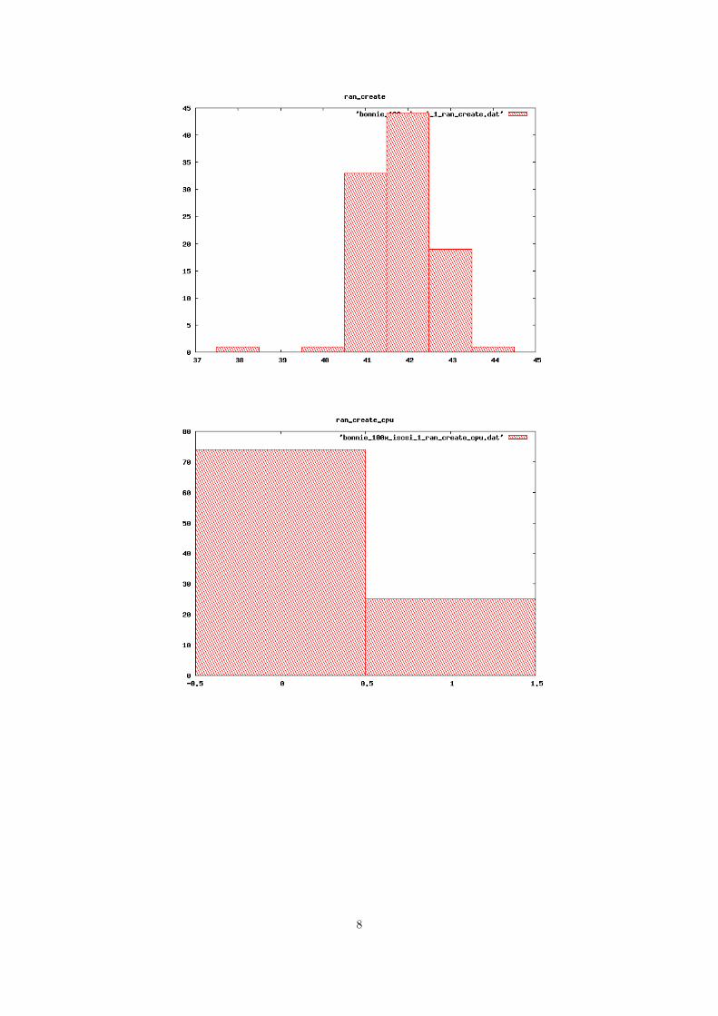
8

9

100x nfs direct
May 19, 2009
Name Mean Median (Mean - Median) Variance Min Max Rangename 0.000 0.000 0.000 nan atlantis atlantis 0file size 4.000 4.000 0.000 nan 4G 4G 0putc 28534.444 28419.000 115.444 611578.954 27089 31697 4608putc cpu 60.212 60.000 0.212 3.238 57 67 10put block 27021.515 26818.000 203.515 1616586.290 24888 30831 5943put block cpu 9.525 9.000 0.525 0.330 9 12 3rewrite 13358.869 13337.000 21.869 47389.791 12861 13942 1081rewrite cpu 2.212 2.000 0.212 0.167 2 3 1getc 23866.505 23721.000 145.505 647568.452 22146 26212 4066getc cpu 44.576 45.000 0.424 24.608 33 55 22get block 25155.343 25202.000 46.657 334903.781 23635 26436 2801get block cpu 5.475 6.000 0.525 0.977 4 8 4seeks 1049.258 1068.800 19.542 6178.578 615.0 1177.2 562.2seeks cpu 1.788 1.000 0.788 8.329 0 13 13num files 16.000 16.000 0.000 nan 16 16 0seq create 38.697 39.000 0.303 0.433 38 40 2seq create cpu 0.000 0.000 0.000 nan 0 0 0seq stat 4472.424 3714.000 758.424 1549846.850 3600 6756 3156seq stat cpu 1.333 1.000 0.333 2.485 0 9 9seq del 77.657 78.000 0.343 2.407 74 79 5seq del cpu 0.000 0.000 0.000 nan 0 0 0ran create 39.101 39.000 0.101 0.273 37 40 3ran create cpu 0.000 0.000 0.000 nan 0 0 0ran stat 4939.737 4005.000 934.737 2523425.547 3916 7943 4027ran stat cpu 0.465 0.000 0.465 1.239 0 9 9ran del 78.404 79.000 0.596 0.726 77 79 2
1

2

3

4

5

6

7

8

9

10

11

12
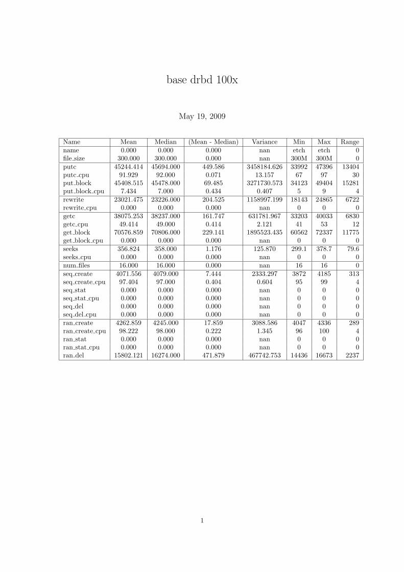
base drbd 100x
May 19, 2009
Name Mean Median (Mean - Median) Variance Min Max Rangename 0.000 0.000 0.000 nan etch etch 0file size 300.000 300.000 0.000 nan 300M 300M 0putc 45244.414 45694.000 449.586 3458184.626 33992 47396 13404putc cpu 91.929 92.000 0.071 13.157 67 97 30put block 45408.515 45478.000 69.485 3271730.573 34123 49404 15281put block cpu 7.434 7.000 0.434 0.407 5 9 4rewrite 23021.475 23226.000 204.525 1158997.199 18143 24865 6722rewrite cpu 0.000 0.000 0.000 nan 0 0 0getc 38075.253 38237.000 161.747 631781.967 33203 40033 6830getc cpu 49.414 49.000 0.414 2.121 41 53 12get block 70576.859 70806.000 229.141 1895523.435 60562 72337 11775get block cpu 0.000 0.000 0.000 nan 0 0 0seeks 356.824 358.000 1.176 125.870 299.1 378.7 79.6seeks cpu 0.000 0.000 0.000 nan 0 0 0num files 16.000 16.000 0.000 nan 16 16 0seq create 4071.556 4079.000 7.444 2333.297 3872 4185 313seq create cpu 97.404 97.000 0.404 0.604 95 99 4seq stat 0.000 0.000 0.000 nan 0 0 0seq stat cpu 0.000 0.000 0.000 nan 0 0 0seq del 0.000 0.000 0.000 nan 0 0 0seq del cpu 0.000 0.000 0.000 nan 0 0 0ran create 4262.859 4245.000 17.859 3088.586 4047 4336 289ran create cpu 98.222 98.000 0.222 1.345 96 100 4ran stat 0.000 0.000 0.000 nan 0 0 0ran stat cpu 0.000 0.000 0.000 nan 0 0 0ran del 15802.121 16274.000 471.879 467742.753 14436 16673 2237
1

2

3

4
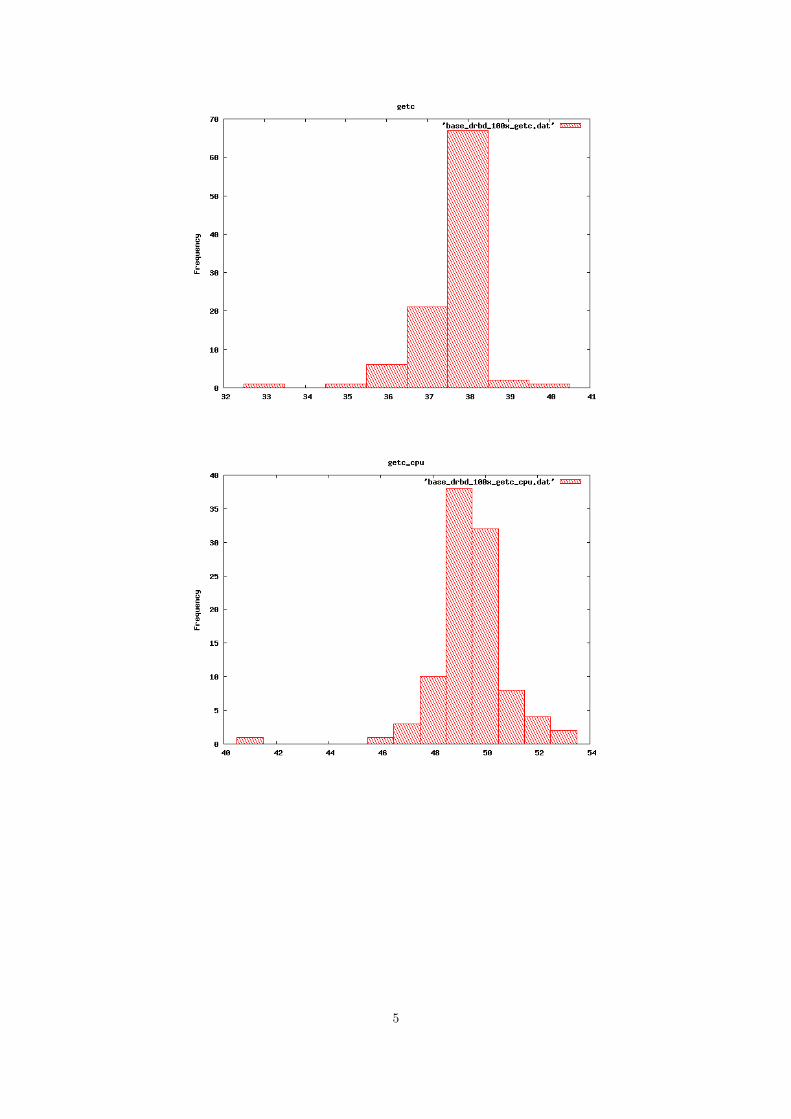
5

6

7

8
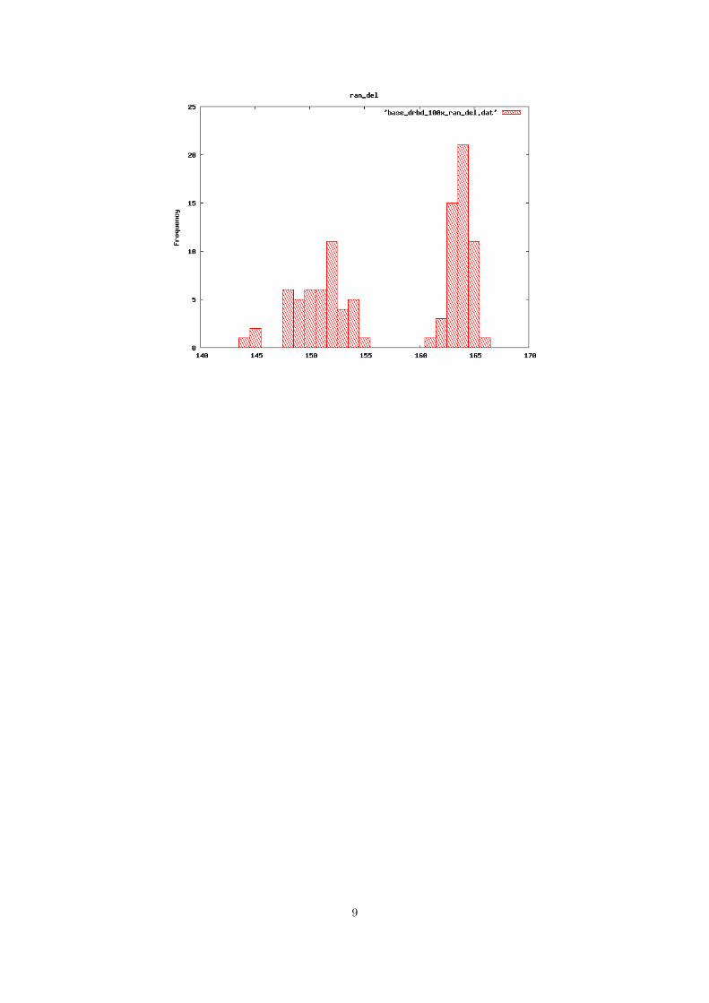
9

100x nfs3of3
May 19, 2009
Name Mean Median (Mean - Median) Variance Min Max Rangename 0.000 0.000 0.000 nan etch etch 0file size 300.000 300.000 0.000 nan 300M 300M 0putc 25321.253 28261.000 2939.747 97671354.229 5540 40616 35076putc cpu 73.343 94.000 20.657 827.700 15 97 82put block 104609.697 111786.000 7176.303 6174875548.393 5495 289875 284380put block cpu 35.444 38.000 2.556 715.863 1 85 84rewrite 53472.293 51444.000 2028.293 1705559591.035 4035 180698 176663rewrite cpu 9.293 8.000 1.293 76.268 0 33 33getc 21595.960 24070.000 2474.040 139606583.554 106 47859 47753getc cpu 54.051 58.000 3.949 935.725 0 95 95get block 141666.374 143731.000 2064.626 13727079249.163 6287 430634 424347get block cpu 4.980 2.000 2.980 37.111 0 23 23seeks 3005.201 306.200 2699.001 23392375.841 0 16365.1 16365.1seeks cpu 2.000 0.000 2.000 17.455 0 17 17num files 16.000 16.000 0.000 nan 16 16 0seq create 2715.535 2929.000 213.465 1122266.734 355 4151 3796seq create cpu 84.000 99.000 15.000 898.929 9 102 93seq stat 0.000 0.000 0.000 nan 0 0 0seq stat cpu 0.000 0.000 0.000 nan 0 0 0seq del 35.293 0.000 35.293 122067.904 0 3494 3494seq del cpu 0.020 0.000 0.020 0.040 0 2 2ran create 3010.030 3037.000 26.970 830162.595 342 4280 3938ran create cpu 90.667 99.000 8.333 512.303 10 100 90ran stat 0.000 0.000 0.000 nan 0 0 0ran stat cpu 0.000 0.000 0.000 nan 0 0 0ran del 11903.657 12049.000 145.343 14317081.256 680 16409 15729
1

2

3

4

5

6

7

8

9

10

11

bonnie 100x iscsi 3of3
May 19, 2009
Name Mean Median (Mean - Median) Variance Min Max Rangename 0.000 0.000 0.000 nan etch3 etch3 0file size 1.000 1.000 0.000 nan 1G 1G 0putc 16258.444 16021.000 237.444 11392432.166 12011 28651 16640putc cpu 34.626 35.000 0.374 42.820 25 59 34put block 15246.657 13532.000 1714.657 8762264.286 12583 21367 8784put block cpu 2.323 2.000 0.323 0.239 2 4 2rewrite 4440.919 4329.000 111.919 172536.923 3675 5821 2146rewrite cpu 0.000 0.000 0.000 nan 0 0 0getc 7730.374 7994.000 263.626 599217.668 5974 11023 5049getc cpu 3.283 3.000 0.283 0.607 2 5 3get block 8996.253 9353.000 356.747 2426084.492 6444 18603 12159get block cpu 0.000 0.000 0.000 nan 0 0 0seeks 231.807 235.000 3.193 7046.147 85.5 482.3 396.8seeks cpu 0.000 0.000 0.000 nan 0 0 0num files 16.000 16.000 0.000 nan 16 16 0seq create 3648.152 3816.000 167.848 168373.785 2434 4102 1668seq create cpu 95.172 96.000 0.828 7.496 86 99 13seq stat 0.000 0.000 0.000 nan 0 0 0seq stat cpu 0.000 0.000 0.000 nan 0 0 0seq del 0.000 0.000 0.000 nan 0 0 0seq del cpu 0.000 0.000 0.000 nan 0 0 0ran create 3683.465 3866.000 182.535 221465.461 2476 4303 1827ran create cpu 95.556 96.000 0.444 7.277 84 100 16ran stat 0.000 0.000 0.000 nan 0 0 0ran stat cpu 0.000 0.000 0.000 nan 0 0 0ran del 13978.010 14799.000 820.990 4517906.879 8749 16253 7504
1

2

3

4

5

6

7

8

9

drbd 100x 2of3
May 7, 2009
Name Mean Median (Mean - Median) Variance Min Max Rangename 0.000 0.000 0.000 nan etch etch 0file size 300.000 300.000 0.000 nan 300M 300M 0putc 10024.525 9206.000 818.525 3988750.613 8181 16904 8723putc cpu 21.141 19.000 2.141 22.950 17 36 19put block 10918.495 10976.000 57.505 745612.129 8558 12888 4330put block cpu 1.657 2.000 0.343 0.225 1 2 1rewrite 7033.495 6891.000 142.495 439018.311 5794 9071 3277rewrite cpu 0.000 0.000 0.000 nan 0 0 0getc 11255.434 11279.000 23.566 604215.599 8971 13099 4128getc cpu 12.121 12.000 0.121 1.157 9 15 6get block 38747.242 36494.000 2253.242 62389843.840 26706 66601 39895get block cpu 0.000 0.000 0.000 nan 0 0 0seeks 147.859 148.500 0.641 70.800 123.4 166.2 42.8seeks cpu 0.000 0.000 0.000 nan 0 0 0num files 16.000 16.000 0.000 nan 16 16 0seq create 3134.626 2996.000 138.626 205190.214 2502 4009 1507seq create cpu 95.455 96.000 0.545 5.056 88 99 11seq stat 0.000 0.000 0.000 nan 0 0 0seq stat cpu 0.000 0.000 0.000 nan 0 0 0seq del 299.283 0.000 299.283 8777880.708 0 29629 29629seq del cpu 0.343 0.000 0.343 11.559 0 34 34ran create 3139.636 2958.000 181.636 202127.565 2509 4216 1707ran create cpu 95.253 95.000 0.253 3.623 89 100 11ran stat 0.000 0.000 0.000 nan 0 0 0ran stat cpu 0.000 0.000 0.000 nan 0 0 0ran del 12651.162 12275.000 376.162 2870622.237 8715 16349 7634
1

2

3

4

5

6

7

8

9

10