marriage and assortative mating: how have the patterns changed
TRANSCRIPT

0
Marriage and Assortative Mating:
How Have the Patterns Changed?
Elaina Rose*
Working Paper No. 22 Center for Statistics and the Social Sciences
University of Washington
December, 2001
[email protected] (206) 543-5237
December, 2001
* Elaina Rose is Associate Professor of Economics, Box 353330, University of Washington, Seattle, WA 98195, e-mail: [email protected]. This research was supported by a grant from the Center for Statistics in the Social Sciences at the University of Washington. Hyung-Jai Choi provided excellent research assistance.

1
I. Introduction
The role of marriage has undergone profound change in recent decades. Divorce and
cohabitation have become commonplace, and age at first marriage has increased for both men and
women. Shifts in marriage patterns would, in general, be expected to be accompanied by changes in the
types of partners that individuals choose when they do form unions. The degree of similarity within
couples is referred to as the degree of “assortative mating.”
The implications of these changes in what Becker [1973] refers to as “marriage markets” are
profound. First, increases in assortative mating with respect to income or wages will tend to exacerbate
the already growing degree of income inequality. Second, declines in marriage and increases in divorce
are associated with increases in the number of single-parent households. To the extent that the well-being
of children is enhanced by living with an intact family, these changes in family structure will have
ramifications for the next generation. Third, changes in the likelihood and role of marriage fuel growth
in women’s labor force participation and human capital accumulation.
The objective of this paper is to document how marriage and assortative mating patterns 1
changed over the period 1970 through 1990 and interpret these changes in terms of the economic theory
of marriage. The analysis uses data from the 1970, 1980 and 1990 Panel Study of Income Dynamics
(PSID).
First, in terms of marriage propensities, I estimate the relationship between education and the
likelihood of marriage, and test for changes in the relationship between decades. I disaggregate by sex,
and by age and find heterogeneity with respect to both.
Next, following the bulk of the literature, I estimate assortative mating patterns in terms of
partners’ education. I find that, overall, husbands and wives became more similar between 1970 and
1980. I find that, on the whole there is hypogamy (i.e., women marrying “down”) with respect to
1 Semantics: I am using the term “assortative mating patterns”, here, to indicate both the degree of similarity within couples (postive/negative assortative mating) as well as the direction of the asymmetry

2
partners’ education,. However, this relationship is non-monotonic. Men are less likely to have
completed 12 years of education than their wives, but men are more likely to have completed 16 years of
education.
Estimates of assortative mating based on own education may be difficult to interpret, as the
education distributions for men and women in the population differ, and have shifted differentially over
time. Therefore, I estimate assortative mating in terms of parents’ as well as own education. I find there
is hypergamy (i.e, women marrying “ up” ) with respect to parents’ education. However, couples are
becoming more similar over time in terms of parents’ education, and the extent of hypergamy has
declined.
Section II outlines the literature on the economics of marriage which motivates this analysis.
Section III describes the data. Section IV presents the results regarding the likelihood of marriage, and
Section V presents the results on assortative mating. Section VI discusses the results and concludes.
II. Theory
The theory of marriage, as developed by Becker [1973, 1974, 1981, 1985] and others specifies
several sources of gains from marriage. First, when one partner has a comparative advantage in market
work relative to home production, a couple can produce more total output by forming a household and
engaging in specialization and exchange. Typically, it is the husband who has the comparative
advantage in the labor market. In one version of this model (Becker, 1985) small initial differences in
relative productivities arise when, say, men are advantaged in the labor market because of gender
discrimination, or when mothers are inherently advantaged in home production in their children’ s early
months. Post-marriage human capital investments (and investments in anticipation of household roles)
reinforce the initial differences in productivity and gender specific returns.
A second source of gains from marriage is production of household public goods. Household
(hypergamy/hypogamy) within couples.

3
public goods – such as a clean living room – or a “ high-quality” child – are those for which one spouse’ s
enjoyment from consuming the good does not interfere with the other spouse’ s ability to enjoy it. Third,
gains from marriage arise when there are economies of scale in production of household goods. For
instance, it is cheaper in terms of both time and purchased inputs to produce two meals together than
separately. Fourth, when one spouse’ s consumption affects the utility of the other, gains from marriage
arise through joint consumption. Fifth, risk averse individuals in two-income households can reap gains
from marriage by sharing risk, similar to the way an investor can reduce risk by diversifying his portfolio
of stocks (Shaw, 1987) . Finally, gains from marriage may arise from institutional factors, such as tax
laws, parents’ approval, and health insurance coverage.
To some extent, each of these benefits may be realized through the market, or through roommate
or cohabiting relationships. However, marriage can reduce transaction costs entailed in market exchange
(Pollak 1995), and provide for greater ability to monitor and enforce agreements than more informal
relationships (Lundberg and Pollak 1995).
There are several respects in which the decline in marriage is consistent with an economic model
of the marriage market. First, as women’ s labor market participation and human capital investment have
increased, potential gains from specialization have declined and the incentive to marry has fallen.
Second, since women tend to marry older men, an increase in fertility creates a “ marriage squeeze” – a
fall in the supply of marriageable men relative to women – about two decades later. So, the post-WWII
baby boom created a marriage squeeze for women from the mid- 1960’ s through the 1980’ s (Grossbard-
Schechtman [1984]). Third, Wilson [1987] cites the deteriorating labor market for less-skilled men as a
key factor in the decline in marriage within the black community. Fourth, some (e.g., Murray [1984 ])
attribute the decline in marriage and increases in non-marital childbearing to increased welfare
generosity.2 Fifth, Akerloff et al [1995] and Akerlof [1998] attribute some part of the decline in
2 Although there is substantial disagreement regarding the magnitudes of the incentive effects of transfer programs (Moffitt [1992]).

4
marriage to the improvement in birth control technology which reduced the stigma associated with non-
marital sex and child-bearing. Finally, changes in family policy such as the liberalization of divorce laws,
as well as shifts in social norms, have reinforced these trends.
The literature on assortative mating (Becker [1981]) addresses the question of who marries
whom, as well as who marries and who remains single. “ Positive (negative) assortative mating” on a
characteristic means that individuals tend to match with partners who are similar (dissimilar) with respect
to that characteristic. Lam [1988] shows that negative assortative mating arises when the gains from
marriage are due to specialization and positive assortative mating arises when gains from marriage are
due to the production household public goods. The net effect is ambiguous if gains arise from both
sources.
Empirical work (Mare [1991], Pencavel [1998], Qian [1998]) has typically focused on assortative
mating with respect to education,3 and finds positive assortative mating with respect to this outcome.
The results that will be presented in Section IV indicate that the decline in the propensity to
marry varies by sex, by age, and by education. Most likely, the magnitudes vary with other observables
and with unobservables, as well. These differences in the effects imply that assortative mating patterns
will, in general, change as well. Whether couples have become more or less similar over time, depends
on which of the source of gains from marriage are most salient, and how the fundamentals generating the
gains have changed. These same factors determine whether there has been an increase or decrease in
hypergamy.
The key source of change in the nature and role of marriage is, arguably, the increase in female
labor force participation and human capital accumulation.4 How would we expect this to have affected
measures of assortative mating based on own education? To the extent that there has been a decline in
the scope for specialization and exchange as women have become more “ like men” in terms of their labor
3 One exception is Brien (1997). 4 Although there are, of course, complex issues of causality here. Certainly, changes in the role of

5
market behavior, 5 we would expect that couples have become more similar, i.e., that assortative mating
has become more positive, over time. Gains arising from the production of public goods, economies of
scale, risk sharing6 and joint consumption will tend to be greater when partners are more similar in terms
of underlying preferences. If the change in the relative distributions of human capital attainment and
labor force participation reflects a shift in underlying preferences, then these four factors will also tend to
lead to an increase in positive assortative mating as well. In terms of the other sources of gains, parental
approval will likely generate more positive assortative mating but the marriage tax and health insurance
coverage practices would tend to work in the opposite direction.
In summary, unless the institutional factors, such as the marriage tax and health insurance
coverage dominate the sum of the others (which seems unlikely), I would expect couples to be becoming
more similar over time – i.e., positive assortative mating to have increased.
What do we expect regarding hypergamy? When gains from marriage are due to specialization
and exchange, men specialize in market work and women in home production, and the returns to
education are greater in market work than in home production then we would expect hypergamy with
respect to education. Gains from production of public goods, economics of scale, joint consumption, or
risk-sharing, would tend to operate symmetrically with respect to husbands and wives. Therefore, there
is no clear reason that any of these factors would generate either hypergamy or hypogamy with respect to
education. So, unless the gains from one of the institutional factors (such as, perhaps, parents’ approval)
are greater when wives marry down and is becoming more important over time (or unless the gains from
one of the factors are greater when wives marry up and is becoming less important over time), then I
would expect hypergamy with respect to education, with the degree of hypergamy declining over time.
marriage have certainly led to changes in female labor market hand human capital outcomes. 5 Empirical work suggesting a decline in the degree of specialization within marriage includes Lundberg and Rose (1998) and Gray (1997). 6 When gains to marriage are due to risk sharing, partners will tend to be dissimilar in terms of income

6
III. Data
The analysis uses data from the Panel Study of Income Dynamics (PSID). The PSID is a panel
data set which follows individuals from an original sample of 5000 households plus splitoff households,
from 1968 until the present time. To capture changes over time, I measure outcomes in 1970, 1980 and
1990. The outcome “ married” is defined as whether an individual is married in a given year. Assortative
mating patterns are defined in terms of couples who are married in a given year, regardless of the
duration of the marriage. These are both, therefore, “ stock measures” of marriage. Future analyses will
look at “ flow measures” such as marriage within a given period or age range, as well as whether
individuals have ever been married.
The PSID’ s “ married pairs indicator” classifies a couple as currently married if they are legally
married, or have cohabited for at least one year.7 Analyses relating to the likelihood of marriage for
individuals use data on original PSID household members, and their children. Individuals who “ married
into” the PSID sample are excluded, as including them would yield a selective and non-representative
sample. Analyses on assortative mating patterns use data on male household heads, and their wives.8
Own education is measured as a continuous variable, “ years of school completed.” Parents’
education is measured in terms of a categorical variable, where the five categories are: (1) 0-5 years of
education, (2) 6-8 years of education, (3) 9-11 years of education, (4) completed high school, (5)
completed college.
IV. Results
The results presented in Table 1 are derived from the following logit model:
streams but not in terms of permanent income. 7 Future work will use the PSID’ s marital history file to distinguish cohabitors from individuals who are legally married. 8 The PSID classifies a husband as the household head in all households that include husbands and wives. There were a few multi-family households which contained two married couples. In these cases, only the primary couple was used but future work will include all married couples.
7
80 90* 1980 1990it it it itM YrsEdu D Dα β γ γ= + + +
80 90* 1980 * 1990it it it it itYrsEdu D YrsEdu Dδ δ ε+ + + (1)
where *itM is a continuous latent variable associated with the likelihood of marriage for individual “ i”
in year “ t” , itYrsEdu is years of completed education, 1980itD is a dummy variable indicating year 1980
or later, and 1990itD is a dummy variable indicating the year 1990. The model is estimated using data
IRU�WKH�\HDUV������������DQG�����������7KH� ¶V�DQG� ¶V��DQG�WKH�UHVSHFWLYH�W-statistics reflect the
incremental effects over the previous decade.
The analyses are performed, by sex, for all individuals age 20-59 in year “ t” and by age groups
20-29, 30-39, 40-49 and 50-59. For the age-disaggregated analyses, no individual or couple is included
in a regression more than once. For the combined sample, individuals may appear more than once.9
Estimates for the entire sample of men are reported in the first column of Table 1.a.. In 1970,
education was associated with a lower likelihood of marriage for men. However, this effect fell
significantly (in absolute value) in each of the subsequent decades. So, by 1990, education had no
significant effect on the likelihood of marriage. The results for women are reported in Table 1.b. There
appears to be no significant relationship between education and the likelihood of marriage in any of the
three years.
The results for the age disaggregated analyses tell a different story. For both men and women in
their 20’ s, more education was associated with a lower likelihood of marriage in 1970. There was no
significant change from 1970 to 1980, but a decline (in absolute value) in the effects for both men and
women between 1980 and 1990.
The pattern is strikingly different for individuals in their 30’ s. Education was associated with a
greater likelihood of marriage for both men and women in 1970 and 1980, but there was a significant
decline in the effect between 1980 and 1990.
8
For men in their 40’ s, there is no significant effect of education, but there is a significantly
positive effect of education for men in their 50’ s in 1980. For women in their 40’ s in 1970 and in their
50’ s in 1980 (i.e., the cohort of women born in the 1920’ s) , there is a significantly positive effect of
education on the likelihood of marriage.
We might expect the effect of education on the likelihood of marriage to be non-linear or even
non-monotonic. For instance, ceteris paribus, if specialization as a motivation for marriage has declined
most dramatically for women with more education, we would expect a greater decline in the effect of
education on the likelihood of marriage for more educated women. So, Tables 2a and 2b report estimates
of the following variant of equation (1):
12 16 80 90* 12 16 1980 1990it it it it itM Plus Plus D Dα β β γ γ= + + + +
12*80 16*8012 * 1980 16 * 1980it it it itPlus D Plus Dδ δ+ +
12*90 16*9012 * 1990 16 * 1990it it it it itPlus D Plus Dδ δ ε+ + + (1’ )
where 12 itPlus is a dummy variable indicating completion of at least twelve years of education, and
16 itPlus is a dummy variable indicating completion of at least sixteen years of education.
The results in Table 2.a indicate that, when the samples are pooled by age, the effect of
education on men’ s likelihood of marriage, and the change in the effect, are significant only with respect
to 16Plus. In 1970, 16Plus was associated with a lower likelihood of marriage, but the effect was
eliminated by 1980 and reversed by 1990. For women, the results in Table 2.b indicate that in 1970,
having at least 12 years of education increased the likelihood of marriage, but that having at least 16
years of education reduced the likelihood of marriage. However, both of these effects were eliminated or
reversed by 1990.
Again, disaggregating by age indicates a different story. For women, in 1970, the positive
coefficient on “ 12Plus carries through for all categories except women in their 20’ s, but the negative
9 In these cases, the standard errors will be understated, and future analyses will adjust standard errors.

9
effect of 16Plus arises solely through the 20-year old category. The pattern for men is similar.
Moreover, the changes over time are quite different for individuals in their 20’ s and individuals age 30
and over. There are several plausible reasons for differences in the patterns for individuals in their 20’ s
and other age groups. For instance, couples in their 20’ s are more likely to be in first marriages, or more
likely to be cohabiting. They are also less likely to have completed their education. Future analyses
based on flow measures of marriage will help clarify the reasons for these differences.
V. Results: Assortative Mating
The top panel of Table 3.a reports estimates of the equation:
80 901980 1990it it it itAbsDiff D Dα β β ε= + + + (2)
where itAbsDiff is the absolute value of the difference between partners’ education. “ Age” refers to the
ZLIH¶V�DJH���³ ´��LV�WKH�DYHUDJH�RI�WKH�RI�WKH�DEVROXWH�YDOXH�RI�WKH�GLIIHUHQFH�LQ�������� 80β and 90β reflect
the change in the average from the previous decade.
The findings in the first column indicate that partners’ education differed, on average, by 1.7
years in 1970. This difference is highly statistically significant (t=49.6). The coefficient on D1980 is -
.23 (t=6.2). This means that in the 1970’ s couples became more similar. However, the coefficient on the
1990 dummy is positive (.07) and significant (t=1.8), indicating that couples became less similar in the
1980’ s.
The results of the disaggregated analysis indicates that couples in all age categories became more
similar in the 1970’ s although the change was significant only for couples in their 20’ s (t=3.0) and 30’ s
(t=5.7), respectively. The increased similarity found for the pooled samples between 1980 and 1990 is
apparent only for couples in their 20’ s (t=2.8).
The second panel reports results of the same analysis, but where the outcome is the raw (i.e., not

10
the absolute value) difference in partners’ education.
For the sample as a whole, and for all age groups except for those in their 20’ s, the intercept is
negative and significant, i.e., men have less education than their wives, or there is “ hypogamy” - women
marrying down - with respect to education. This is inconsistent with the conjecture offered in Section II,
that, because of specialization and exchange, women will tend to marry up with respect to education.
For the sample as a whole, and for couples in their 30’ s the difference fell in the 1970’ s. In fact, for
couples in their 30’ s, the difference in 1970 was completely wiped out by 1980, although it grew again in
the subsequent decade.
The interpretation of estimates of changes in the assortative mating patterns based on husbands’
and wives’ education is clouded by the fact that the distributions of men’ s and women’ s education are
different, and have shifted differentially over time. Historically, women have been more likely to
graduate from high school, but men have been more likely to graduate from college. However, the
patterns have shifted dramatically over the period. College graduation rates have increased substantially
more for women than for men since 1960, and women are now more likely to attend, and graduate from
college, than men.
How would these shifts affect the interpretation of the results? The finding of hypogamy with
respect to own education may be attributed to the greater supply of women relative to men high school
graduates, rather than hypogamy with respect to an underlying unobservable such as preferences or
endowments. The increased similarity of couples in terms of education might reflect increased similarity
in the distributions of education of women relative to men, rather than increased similarity in terms of
underlying preferences.
While the distributions of women’ s and men’ s educations are different, and have changed
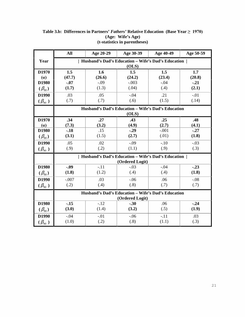
differentially over time, the same would not be true for, say, partners’ fathers’ education. For this
reason, I repeat the analysis in Table 3.a with the outcomes being partners’ fathers’ education (Table 3.b)
11
and partners’ mothers’ education (Table 3.c).
As parents’ education is measured as a categorical variable on the PSID, the interpretation of the
magnitudes of the estimates from Tables 3.b and 3.c differ from those of Table 3.a. Each unit of the
dependent variable represents one of the five education categories, rather than a year of education. Each
equation is estimated under OLS and as an ordered logit. While the ordered specification is more
appropriate, it does not produce estimates of the constant.
The results in Table 3.b indicate that, on average, in 1970, partners’ fathers’ education differed
by between 1.5 and 1.7 categories. The gap between fathers’ education narrowed between 1970 and
1980, for each category, but the change was significant only for the pooled sample, and for couples age
50-59.
The estimates for the raw differences reported in the second panel indicate that, on average,
husbands’ fathers are more educated that wives fathers’ . So, while there is hypogamy with respect to
own education, there is hypergamy; i.e., women marrying up, with respect to father’ s education.
However, the gap narrowed significantly for the pooled sample, and for couples in their 30’ s and 50’ s.
The results for the ordered specifications are consistent with the OLS estimates. Both the finding of
hypergamy overall, and a decline in hypergamy over time, are consistent with the conjectures.
The analysis is repeated for partners’ mothers in Table 3.c. There is hypergamy with respect to
mother’ s education, although the results are weaker – possibly because there is less variation in partner’ s
mothers’ education than in partners’ fathers’ variation. The raw differences fell for couples in their 30’ s
between 1970 and 1980, and for couples in their 40’ s between 1980 and 1990 – i.e., for the cohort of
couples in which the wife was born in 1940’ s.
Tables 4 through 6 present a series of 2x2 contingency tables which allow for non-linearities in
the assortative mating patterns. Table 4.a reports the proportion of couples in which neither completed
12 years of education (“ W_12+” = 0 and “ H_12+” = 0), only the wife completed 12 years of education

12
(“ W_12+” = 1 and “ H_12+” = 0), only the husband completed 12 years of education (“ W_12+” = 0 and
“ H_12+” = 1), and both completed 12 years of education (“ W_12+” = 1 and “ H_12+” = 1), by wife’ s
age, and by year. A greater sum of the diagonal elements on a 2x2 table indicates more similarity within
couples, and a greater difference between the upper (northeast) off-diagonal element to the lower
(southwest) off-diagonal element indicates more hypergamy.10
The results in Table 4.a indicate little change in the patterns for couples age 20-29. The
percentage of couples in which either both, or neither completed 12 years of education was 80.7 in 1970,
82.3 in 1980, and 81.2 in 1990. The difference in the off-diagonals was –5 percentage points in 1970, -
3.9 in 1980 and -3.4 in 1990. So, overall, there is hypogamy with respect to “ 12Plus” , but the change has
been small, and there has been little change in the degree of similarity of spouses age 20-29 with respect
to this outcome.
The results for the other age categories are different, however. For couples in their 30’ s, 72.1
percent had the same outcome in 1970, but 83.6 percent did in 1990. For couples in their 40’ s, the
figures are 78.3 percent in 1970 and 82.7 percent in 1990, and for couples in their 50’ s, the figures are
77.8 percent in 1970 and 88.4 percent in 1990. So, couples in their 30’ s, 40’ s and 50’ s have become
more similar over the period, at least in terms of achieving twelve years of education.
The structure of Table 4.b is identical to that of Table 4.a, but the outcome is whether the
partners completed at least 16 years of education. Overall, couples are becoming somewhat more
dissimilar with respect to this outcome. 88.1 percent of the couples in 1970 report that either both or
neither have at least 16 years of education, but the figure is 83.1 percent in 1990. The decline is present
for all age groups except couples in their 20’ s.
For the most part, there is hypergamy with respect to college education. In virtually all
subsamples, it is more likely that the husband has at least 16 years of education and the wife does not,
10 Items for the research agenda include tests of significant differences in the off-diagonals, and significant changes in assortative mating and hypergamy over time.
13
than vice versa. In most cases, the degree of hypergamy is declining as well. For couples in their 20’ s in
1970, it was three times as likely for the husband to have 16Plus and the wife not, than vice versa, while
in 1990 this age group exhibited hypogamy. Similar declines are apparent for couples in their 30’ s and
40’ s.
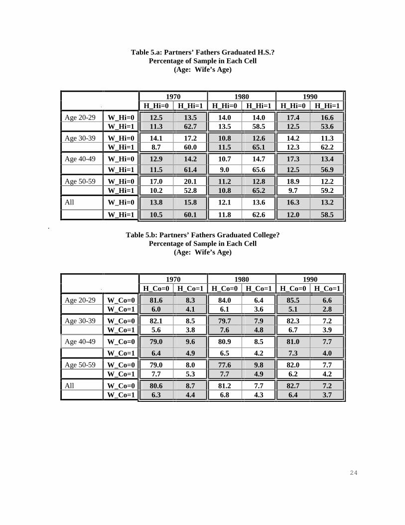
Tables 5.a and 5.b report the results of the same analysis, but with respect to fathers’ education.
Overall, there is hypergamy with respect to these outcomes. There has been little change in the degree
of hypergamy or assortative mating over time.
The outcomes in Tables 6.a and 6.b pertain to mothers’ education. Again there is evidence of
hypergamy with respect to both outcomes. Couples in their 20’ s appear to have become slightly less
similar in terms of mothers’ high school completion, but couples in the other categories appear to have
become somewhat more similar.11
VI. Conclusion and Directions for Future Research
The analysis has uncovered several interesting patterns with respect to marriage market
outcomes. First, there is substantial heterogeneity in the relationships by age and gender. In many cases,
the marriage and partner choice outcomes for people in their 20’ s behaved quite differently from those at
older ages. For instance, education is associated with a lower likelihood of marriage for both men and
women in their 20’ s, but a greater likelihood of marriage for men and women in their 30’ s. One goal of
future work will be to uncover the source of this heterogeneity by using flow as well as stock measures of
marriage, and distinguishing first vs. later marriages and marriages with and without children.
In terms of gender, for example, the positive effect of high school completion on the likelihood
of marriage for women in 1970and 1980 was completely eliminated by 1990, although there was no
change in the effect of education for men in the same age range.
Second, the effects of education on the likelihood of marriage are non-monotonic. For instance,

14
for the sample of women, pooled by age, having at least 12 years of education is associated with a greater
likelihood of marriage, but moving on to 16 years of education reduces the likelihood of marriage.
Third, there is hypogamy with respect to own education when the variable is measured linearly.
However, the patterns are non-monotonic. While husbands are less likely to have achieved 12 years of
education than their wives, they are more likely than their wives to have completed 16 years of
education. Couples are becoming more similar in terms of the first outcome, but somewhat less similar
in terms of the latter.
Fourth, the assortative mating patterns are very different when measured in terms of parents’
education. While there is hypogamy overall with respect to own education, there is hypergamy in terms
of both partners’ fathers’ education, and partners’ mother’ s education. The fact that the differences in
estimates based on own education and estimates based on parents’ education are so stark suggests that
the problem of the differing distributions of education of men and women in the population is important.
Failure to attend to this issue when interpreting assortative mating patterns based on own characteristics
may lead to very misleading conclusions about the behavior of marriage markets.12
Fifth, there is evidence that individuals are becoming more similar in terms of parents’ education,
and that hypergamy with respect to parents’ education is declining. This is as expected when gains from
marriage are due to specialization and exchange, and parents’ education reflects labor market human
capital.
There are several other ways in which this analysis will be developed. First, cohabitors can be
11 And I can’ t say yet if these changes are statistically significant. 12 It might also be argued that parents’ education reflects underlying preferences and family background to a greater extent than own education, and own education proxies for labor market productivity. Gains from production of public goods, economies of scale, joint consumption, risk sharing and some institutional factors are more likely to be related to preferences and background, and gains from specialization and exchange result from differences in labor market activity. Therefore, we would expect less similarity in estimates based on own education as that captures more of the dimension of assortative mating based on specialization and exchange, while estimates based on parents’ education capture more of the dimension based on the other factors. However, under the specialization model, hypogamy with respect to own education would imply a tendency for women to specialize in market work.
15
distinguished from legally married couples in order to have a more consistently defined measure of
marriage and to test models of alternative union types. For instance, some (e.g., Bumpass et al [1991])
argue that for some couples cohabitation is a substitute for marriage. If this were the case, then changes
in the likelihood of marriage based on measures that exclude cohabitors would likely be larger than those
which include cohabitors. As there is less of a role for specialization and exchange for cohabitors than
for legally married couples, estimates of assortative mating based on legally married couples only would
likely indicate less similarity, and more hypergamy than the estimates presented here.
Second, marriages with children can be distinguished from those without. I would expect
marriages with children to be more specialized, as the birth of a child increases the value of a woman’ s
time in home production (Lundberg and Rose, 1998, 2000a, 2000b).
Third, the sample can be expanded to include data up to 1990 in order to estimate changes over a
longer time period. Fourth, alternative data sets can be employed to validate and extend these findings.
For instance, the U.S. Census provides a much larger sample which will produce more precise estimates
of some of the effects.
Finally, the objective of this paper is to describe the changes in marriage and assortative mating
patterns and interpret the findings in terms of the economic theory of marriage. It is the first stage in a
larger project in which explicit testing of alternative models of marriage will be undertaken. One aim of
the larger project is to express the theory outlined in Section II in terms of a more formal model of the
marriage market. In terms of the empirical analysis, observables such as AFDC and family policy
variables, marriage market conditions, and additional individual and family characteristics will be
entered into equations (1) and (2). Estimating the effects of these fundamentals on the likelihood of
marriage and assortative mating patterns, and studying how each one contributes to the variation in
marriage, assortative mating, and hyprgamy, will help illuminate our understanding of role of marriage,
and how it has changed in the latter part of the twentieth century.

16
References
Akerlof, George A, Janet L. Yellen and Michael L. Katz (1996) “ An Analysis of Out-of-Wedlock Childbearing in the United States” Quarterly Journal of Economics 111:2, 277-317. Akerlof, George A.(1998) “ Men without Children” Economic Journal 108 287-309. Becker, Gary S. (1973) “ A Theory of Marriage: Part I” Journal of Political Economy 81:4, 813-46. Becker , Gary S. (1974) “ A Theory of Marriage: Part II” Journal of Political Economy 82:2, S11-S26. Becker, Gary S. (1981) A Treatise on the Family (Cambridge: Harvard University Press). Becker, Gary S. (1985) “ Human Capital, Effort, and the Sexual Division of Labor” Journal of Labor Economics 81:4, 813-46. Brien, Michael J (1997) “ Racial Differences in Marriage and the Role of Marriage Markets” Journal of Human Resources 32:4, 741-78. Bumpass, L. L., J.J. Sweet and Andrew Cherlin (1991) “ The Role of Cohabitation in Declining Rates of Marriage” Journal of Marriage and the Family 53, 913-27. Easterlin, Richard A. (1980) Birth and Fortune (New York: Basic Books). Gray, Jeffrey S. (1997) “ The Fall in Men's Return to Marriage: Declining Productivity Effects or Changing Selection?” Journal of Human Resources 32:3, 481-504. Grossbard-Schechtman (1993) On the Economics of Marriage: A Theory of Marriage, Labor and Divorce (Westview Press, Boulder, CO). Jacobsen, Joyce, (1998) The Economics of Gender (New York: Blackwell). Lam, David (1988) “ Marriage Markets and Assortative Mating with Household Public Goods: Theoretical Results and Empirical Implications” Journal of Human Resources 23(4) 462-87. Lundberg, Shelly and Robert A. Pollak (1995) “ Bargaining and Distribution in Marriage” Journal of Economic Perspectives 10:4, 139-58. Lundberg and Rose (1998) “ The Determinants of Specialization within Marriage” , mimeo, University of Washington. Lundberg and Rose (1999) “ The Effects of Sons and Daughters on Men’ s Labor Supply and Wages,” mimeo, University of Washington. Lundberg and Rose (2000a) “ Parenthood and the Earnings of Married Men and Women,” Labour Economics, 7:6, November, 689-710. Lundberg and Rose (2000b) “ ‘A Boy Needs a Father’ : Child Gender and the Transition to Marriage

17
from Single Motherhood,” mimeo, University of Washington. Mare, Robert (1991) “ Five Decades of Educational Assortative Mating, American Sociological Review 56 15-32. Moffitt, Robert A. (1992) “ Incentive Effects of the U.S. Welfare System: A Review” Journal of Economic Literature 30, 1-61. Moffitt Robert A. (1990) “ The Effect of the U.S. Welfare System on Marital Status,” Journal of Public Economics 41:1, 101-24. Murray, Charles (1984) Losing Ground: American Social Policy 1950-1980 (Basic Books: New York, NY). Pencavel, John (1998) “ Assortative Mating by Schooling and the Work Behavior of Wives and Husbands” American Economic Review 88:2, 326-29. Pollak, Robert A., “ A Transaction Cost Approach to Families and Households” Journal of Economic Literature 23:2 581-608. Qian , Zhenchao (1998) “ Changes in Assortative Mating: The Impact of Age and Education, 1970-1990” Demography 35:3, 279-92. Rosenzweig, Mark R. (1999) “ Welfare, Marital Prospects and Non-Marital Childbearing” mimeo, Penn. Shaw, Kathryn (1987) “ The Quit Propensity of Married Men” Journal of Labor Economics 5:4, 533-60. Wilson, William Julius (1987) The Truly Disadvantaged (University of Chicago Press, Chicago IL).

18
Table 1.a: Effect of Men’s Education on Likelihood of Marriage (Logit)
Base category: 1970, unless otherwise specified (t-statistics in parentheses)
All Age 20-29
Age 30-39
Age 40-49
Age 50-59*
Yrs. Edu
-.016 (4.8)
-.02 (3.1)
.009 (1.7)
.005 (1.1)
.01 (2.4)
Yrs. Edu * D1980
.008 (1.9)
.005 (.5)
.005 (.7)
.002 (.3)
Yrs. Edu * D1990
.01 (2.8)
.014 (1.9)
-.011 (1.7)
-.001 (.25)
-.007 (1.3)
D1980 -.214 (4.0)
-.20 (1.7)
-.183 (1.9)
-.106 (1.5)
D1990 -.142 (3.2)
-.24 (2.4)
.040 (.47)
-.02 (.3)
.043 (.7)
N 10498 4079 3081 2106 1232
Table 1.b: Effect of Women’s Education on Likelihood of Marriage (Logit)
Base category: 1970, unless otherwise specified (t-statistics in parentheses)
All Age 20-29
Age 30-39
Age 40-49
Age 50-59*
Yrs. Edu
.004 (1.2)
-.012 (1.7)
.018 (2.6)
.021 (3.5)
.013 (2.1)
Yrs. Edu * D1980
-.005 (1.0)
-.009 (1.0)
.000 (.01)
.004 (.5)
Yrs. Edu * D1990
-.001 (.3)
.013 (1.7)
-.021 (2.9)
-.024 (3.2)
-.000 (.02)
D1980 -.029 (.5)
-.025 (.2)
-.047 (.4)
-.118 (1.1)
D1990 -.008 (.2)
-.187 (1.9)
.192 (2.0)
.267 (2.8)
-.038 (.44)
N 12480 4499 3658 2696 1627
* Base Year is 1980.

19
Table 2.a: Effect of Education on Mens’ Likelihood of Marriage (Non-Linear) Base category: 1970, unless otherwise specified
All Age
20-29 Age
30-39 Age
40-49 Age
50-59* 12 +
-.036 (1.5)
-.012 (.2)
.108 (2.7)
.037 (1.1)
.097 (2.9)
16 +
-.087 (3.1)
-.114 (2.8)
-.004 (.08)
-.034 (.7)
-.052 (1.1)
12 + * D1980
.018 (.6)
.041 (.7)
-.016 (.3)
.098 (2.1)
16 + * D1980
.071 (2.0)
-.033 (.6)
.029 (.5)
-.045 (.7)
12 + * D1990
.031 (1.3)
.009 (.22)
-.032 (.7)
-.115 (2.7)
-.023 (.5)
16 + * D1990
.123 (4.4)
.20 (3.7)
-.006 (.2)
.14 (2.9)
.03 (.5)
D1980 -.147 (6.1)
-.174 (3.5)
-.177 (2.6)
-.135 (4.2)
D1990 -.067 (3.4)
-.088 (2.4)
-.072 (1.8)
.007 (.2)
-.033 (1.1)
Table 2.b: Effect of Education on Womens’ Likelihood of Marriage (Non-Linear)
Base category: 1970, unless otherwise specified
All Age 20-29
Age 30-39
Age 40-49
Age 50-59*
12 +
.101 (4.7)
.048 (1.2)
.133 (3.7)
.158 (4.4)
.13 (3.5)
16 +
-.079 (2.5)
-.14 (3.2)
.055 (.9)
.021 (.3)
-.034 (.5)
12 + * D1980
-.028 (1.0)
.008 (.2)
.007 (.14)
-.019 (.4)
16 + * D1980
.035 (.9)
.013 (.2)
-.026 (.4)
.059 (.7)
12 + * D1990
-.061 (2.7)
-.058 (1.3)
-.15 (3.1)
-.104 (2.2)
-.016 (.3)
16 + * D1990
.11 (3.6)
.18 (3.5)
.037 (.7)
-.035 (.5)
.037 (.4)
D1980 -.076 (3.4)
-.154 (3.3)
-.054 (1.3)
-.055 (1.5)
D1990 .012 (.6)
.005 (.12)
.034 (.8)
.055 (1.5)
-.037 (1.0)
* Base Year is 1980.

20
Table 3.a: Differences in Partners’ Relative Education (Base Year: �������
(Age: Wife’s Age) (t-statistics in parentheses)
All Age 20-29 Age 30-39 Age 40-49 Age 50-59 Year ��+XVEDQG¶V�(GXFDWLRQ�– Wife’s Education
(OLS) D1970 � �
1.7 (49.6)
1.4 (25.0)
1.9 (28.4)
1.8 (24.8)
1.9 (20.3)
D1980 ( 80β )
-.28 (6.2)
-.21 (3.0)
-.47 (5.7)
-.07 (.7)
-.07 (.5)
D1990 ( 90β )
.07 (1.8)
.18 (2.8)
.07 (1.0)
-.12 (1.2)
-.12 (1.0)
Husband’s Education – Wife’s Education (OLS)
D1970 � �
-.32 (6.7)
-.07 (.9)
-.34 (3.9)
-.41 (4.1)
-.56 (4.3)
D1980 ( 80β )
.16 (2.6)
-.06 (.7)
.34 (3.0)
.17 (1.1)
.13 (.8)
D1990 ( 90β )
.016 (.3)
-.10 (1.1)
-.20 (2.1)
.15 (1.1)
.51 (3.1)
21
Table 3.b: Differences in Partners’ Fathers’ Relative Education (Base Year �������� (Age: Wife’s Age)
(t-statistics in parentheses)
All Age 20-29 Age 30-39 Age 40-49 Age 50-59
Year | Husband’s Dad’s Education – Wife’s Dad’s Education | (OLS)
D1970 � �
1.5 (47.7)
1.6 (26.6)
1.5 (24.2)
1.5 (23.4)
1.7 (20.8)
D1980 ( 80β )
-.07 (1.7)
-.09 (1.3)
-.003 (.04)
-.04 (.4)
-.21 (2.1)
D1990 ( 90β )
.03 (.7)
.05 (.7)
-.04 (.6)
.21 (1.5)
-.01 (.14)
Husband’s Dad’s Education – Wife’s Dad’s Education (OLS)
D1970 � �
.34 (7.3)
.27 (3.2)
.43 (4.9)
.25 (2.7)
.48 (4.1)
D1980 ( 80β )
-.18 (3.1)
.15 (1.5)
-.29 (2.7)
-.001 (.01)
-.27 (1.8)
D1990 ( 90β )
.05 (.9)
.02 (.2)
-.09 (1.1)
-.10 (.9)
-.03 (.3)
| Husband’s Dad’s Education – Wife’s Dad’s Education | (Ordered Logit)
D1980 ( 80β )
-.09 (1.8)
-.11 (1.2)
-.03 (.4)
-.04 (.4)
-.23 (1.8)
D1990 ( 90β )
-.007 (.2)
.03 (.4)
-.06 (.8)
.06 (.7)
-.08 (.7)
Husband’s Dad’s Education – Wife’s Dad’s Education (Ordered Logit)
D1980 ( 80β )
-.15 (3.0)
-.12 (1.4)
-.30 (3.2)
.06 (.5)
-.24 (1.9)
D1990 ( 90β )
-.04 (1.0)
-.01 (.2)
-.06 (.8)
-.11 (1.1)
.03 (.3)

22
Table 3.c: Differences in Partners’ Mothers’ Relative Education (Base Year �������� (Age: Wife’s Age)
(t-statistics in parentheses)
All Age 20-29 Age 30-39 Age 40-49 Age 50-59
Year | Husband’s Mom’s Education – Wife’s Mom’s Education | (OLS)
D1970 � �
1.3 (45.2)
1.3 (25.2)
1.3 (23.2)
1.4 (23.9)
1.3 (17.0)
D1980 ( 80β )
-.02 (.6)
-.07 (1.1)
.08 (1.1)
-.13 (1.6)
.07 (.8)
D1990 ( 90β )
.03 (.8)
.094 (1.7)
-.07 (1.3)
.12 (1.6)
-.05 (.7)
Husband’s Mom’s Education – Wife’s Mom’s Education (OLS)
D1970 � �
.18 (4.3)
.09 (1.2)
.33 (4.2)
.12 (1.4)
.17 (1.6)
D1980 ( 80β )
-.06 (1.2)
.06 (.6)
-.32 (3.1)
.09 (.8)
-.07 (.5)
D1990 ( 90β )
-.01 (.3)
-.01 (.2)
.12 (1.5)
-.22 (2.2)
.06 (.5)
| Husband’s Mom’s Education – Wife’s Mom’s Education | (Ordered Logit)
D1980 ( 80β )
-.01 (.3)
-.10 (1.1)
.13 (1.3)
-.15 (1.4)
.13 (1.0)
D1990 ( 90β )
.02 (.4)
.09 (1.1)
.12 (-1.6)
.16 (1.7)
-.09 (.8)
Husband’s Mom’s Education – Wife’s Mom’s Education (Ordered Logit)
D1980 ( 80β )
-.06 (1.3)
.06 (.6)
-.30 (3.1)
.089 (.8)
-.09 (.7)
D1990 ( 90β )
-.01 (.3)
-.02 (.2)
.11 (1.4)
-.21 (2.2)
.07 (.7)

23
Table 4.a: Partners Have 12Plus Years of Education? Percentage of Sample in Each Cell
(Age: Wife’s Age)
1970 1980 1990 H_12+
= 0 H_12+
= 1 H_12+
= 0 H_12+
= 1 H_12+ =
0 H_12+
= 1
Age 20-29 W_12+ = 0 11.8 7.2 5.4 6.9 6.2 7.7 W_12+ = 1 12.2 68.9 10.8 76.9 11.1 75.0
Age 30-39 W_12+ = 0 22.0 10.4 7.0 5.9 8.2 4.9 W_12+ = 1 17.5 50.1 10.1 77.0 8.6 75.4
Age 40-49 W_12+ = 0 33.4 7.7 19.2 9.1 13.7 6.2
W_12+ = 1 14.0 44.9 15.5 56.2 11.0 69.0
Age 50-59 W_12+ = 0 41.0 7.6 27.4 8.8 25.7 9.9 W_12+ = 1 13.5 37.8 16.4 47.4 11.7 52.7
All W_12+ = 0 24.2 7.3 11.1 6.7 11.4 6.4 W_12+ = 1 15.4 53.0 12.7 69.5 10.2 72.0
.
Table 4.b: Partners Have 16Plus Years of Education? Percentage of Sample in Each Cell
(Age: Wife’s Age)
1970 1980 1990 H_16+ =
0 H_16+ =
1 H_16+ =
0 H_16+ =
1 H_16+ =
0 H_16+ =
1
Age 20-29 W_16+ = 0 72.8 12.0 79.2 7.2 80.1 6.2
W_16+ = 1 4.0 11.2 6.1 7.6 7.1 6.6
Age 30-39 W_16+ = 0 82.5 8.8 65.6 12.1 71.4 9.6 W_16+ = 1 2.2 6.5 6.0 16.3 8.9 10.1
Age 40-49 W_16+ = 0 82.7 8.8 79.9 10.2 68.6 11.4
W_16+ = 1 2.2 6.3 3.1 6.8 6.2 13.8
Age 50-59 W_16+ = 0 88.2 5.7 81.6 8.8 81.5 10.3 W_16+ = 1 2.5 3.7 2.5 7.1 2.9 5.3
All W_16+ = 0 80.3 8.7 75.2 8.9 73.2 9.0 W_16+ = 1 3.2 7.8 5.7 10.3 7.3 9.9
24
Table 5.a: Partners’ Fathers Graduated H.S.? Percentage of Sample in Each Cell
(Age: Wife’s Age)
1970 1980 1990 H_Hi=0 H_Hi=1 H_Hi=0 H_Hi=1 H_Hi=0 H_Hi=1
Age 20-29 W_Hi=0 12.5 13.5 14.0 14.0 17.4 16.6 W_Hi=1 11.3 62.7 13.5 58.5 12.5 53.6
Age 30-39 W_Hi=0 14.1 17.2 10.8 12.6 14.2 11.3 W_Hi=1 8.7 60.0 11.5 65.1 12.3 62.2
Age 40-49 W_Hi=0 12.9 14.2 10.7 14.7 17.3 13.4
W_Hi=1 11.5 61.4 9.0 65.6 12.5 56.9
Age 50-59 W_Hi=0 17.0 20.1 11.2 12.8 18.9 12.2 W_Hi=1 10.2 52.8 10.8 65.2 9.7 59.2
All W_Hi=0 13.8 15.8 12.1 13.6 16.3 13.2
W_Hi=1 10.5 60.1 11.8 62.6 12.0 58.5
. Table 5.b: Partners’ Fathers Graduated College?
Percentage of Sample in Each Cell (Age: Wife’s Age)
1970 1980 1990 H_Co=0 H_Co=1 H_Co=0 H_Co=1 H_Co=0 H_Co=1
Age 20-29 W_Co=0 81.6 8.3 84.0 6.4 85.5 6.6 W_Co=1 6.0 4.1 6.1 3.6 5.1 2.8
Age 30-39 W_Co=0 82.1 8.5 79.7 7.9 82.3 7.2 W_Co=1 5.6 3.8 7.6 4.8 6.7 3.9
Age 40-49 W_Co=0 79.0 9.6 80.9 8.5 81.0 7.7
W_Co=1 6.4 4.9 6.5 4.2 7.3 4.0
Age 50-59 W_Co=0 79.0 8.0 77.6 9.8 82.0 7.7 W_Co=1 7.7 5.3 7.7 4.9 6.2 4.2
All W_Co=0 80.6 8.7 81.2 7.7 82.7 7.2 W_Co=1 6.3 4.4 6.8 4.3 6.4 3.7

25
Table 6.a Partners’ Mothers Graduated H.S.?
Percentage of Sample in Each Cell (Age: Wife’s Age)
1970 1980 1990 H_Hi=0 H_Hi=1 H_Hi=0 H_Hi=1 H_Hi=0 H_Hi=1
Age 20-29 W_Hi=0 9.5 11.3 9.0 12.9 13.2 13.4 W_Hi=1 8.2 71.0 9.1 69.1 10.8 62.3
Age 30-39 W_Hi=0 9.7 15.1 6.4 10.8 11.7 10.7
W_Hi=1 8.0 67.3 7.6 75.2 8.6 69.0
Age 40-49 W_Hi=0 7.6 12.3 7.4 12.0 13.9 10.4
W_Hi=1 9.7 70.4 8.1 72.5 10.3 65.3
Age 50-59 W_Hi=0 12.9 16.0 7.5 10.2 17.3 11.2
W_Hi=1 10.1 61.0 8.8 73.5 8.5 63.1
All W_Hi=0 9.6 13.4 7.7 11.7 13.3 11.3 W_Hi=1 8.8 68.2 8.5 72.1 9.5 65.8
. Table 6.b: Partners’ Mothers Graduated College?
Percentage of Sample in Each Cell (Age: Wife’s Age)
1970 1980 1990 H_Co=0 H_Co=1 H_Co=0 H_Co=1 H_Co=0 H_Co=1
Age 20-29 W_Co=0 91.3 4.3 89.7 4.8 90.9 4.6 W_Co=1 3.5 1.0 3.5 2.1 3.7 1.0
Age 30-39 W_Co=0 90.3 6.3 89.7 5.0 88.3 5.9 W_Co=1 2.4 1.0 4.2 1.1 3.8 2.0
Age 40-49 W_Co=0 87.0 7.8 90.0 6.3 90.1 4.4
W_Co=1 4.1 1.2 2.8 1.0 4.3 1.2
Age 50-59 W_Co=0 92.5 3.8 86.5 8.0 90.6 6.1
W_Co=1 2.2 1.6 4.3 1.2 2.2 1.1
All W_Co=0 90.1 5.7 89.2 5.6 89.7 5.3 W_Co=1 3.2 1.1 3.7 1.5 3.4 1.4