markov property for a function of a markov chain: a linear algebra approach

Linear Algebra and its Applications 404 (2005) 85–117www.elsevier.com/locate/laa

Markov property for a function of a Markovchain: A linear algebra approach

Leonid Gurvits a,1, James Ledoux b,∗,2aLos Alamos National Laboratory, NM 87545, USAbCentre de Mathématiques INSA & IRMAR, France

Received 11 May 2004; accepted 10 February 2005Available online 30 March 2005

Submitted by S. Kirkland

Abstract

In this paper, we address whether a (probabilistic) function of a finite homogeneous Mar-kov chain still enjoys a Markov-type property. We propose a complete answer to this questionusing a linear algebra approach. At the core of our approach is the concept of invariance of a setunder a matrix. In that sense, the framework of this paper is related to the so-called “geometricapproach” in control theory for linear dynamical systems. This allows us to derive a collectionof new results under generic assumptions on the original Markov chain. In particular, weobtain a new criterion for a function of a Markov chain to be a homogeneous Markov chain.We provide a deterministic polynomial-time algorithm for checking this criterion. Moreover,a non-standard notion of observability for a linear system will be used. This allows one toshow that the set of all stochastic matrices for which our criterion holds, is nowhere dense inthe set of stochastic matrices.© 2005 Elsevier Inc. All rights reserved.

∗ Corresponding author.E-mail address: [email protected] (J. Ledoux).

1 Leonid Gurvits dedicates this paper to the memory of Alexander Mihailovich Zaharin. Sasha was oneof the pioneers of the Lumpability research and the most fun guy I ever knew.

2 Address: Institut National des Sciences Appliquees, 20 avenue des Buttes de Coësmes, 35043 RennesCedex, France.

0024-3795/$ - see front matter � 2005 Elsevier Inc. All rights reserved.doi:10.1016/j.laa.2005.02.007

www.elsevier.com/locate/laa

mailto:[email protected]

86 L. Gurvits, J. Ledoux / Linear Algebra and its Applications 404 (2005) 85–117

AMS classification: 15A51; 47A15; 60J10; 93B07

Keywords: kth-order Markov chain; Rogers–Pitman matrix; Hidden Markov chain

1. Introduction

Markov models are probably the most common stochastic models for dynamicalsystems. However, when a Markov model approach is chosen, one can expect the fol-lowing issues to appear. First, computational time explosion as dimensions increase.Second, statistical properties related to a functional of the initial Markov model willbe the quantities of interest, rather than the initial Markov model itself.

As a result, one either has to derive a model reduction to address the first issue,or deal with a functional of a Markov chain to address the second. Let us consider adiscrete-time homogeneous Markov chain (Xn) as our initial Markov model. We as-sume that each random variable Xn is X-valued, where X is the finite set {1, . . . , N}and is called the state space of the Markov chain (Xn). A basic way to reducethe dimension of this Markov model is to lump or collapse some states into a sin-gle “mega-state”. Thus, we obtain a partition {C(1), . . . , C(M)} of X into M < N

classes. Given such a partition, we define a map ϕ from X into Y := {1, . . . , M} by

∀k ∈ X, ∀l ∈ Y, ϕ(k) := l ⇐⇒ k ∈ C(l).

The map ϕ will be referred to as a lumping map. Then, we are interested in the newprocess (ϕ(Xn)) defined by

ϕ(Xn) = l ⇐⇒ Xn ∈ C(l).

Each random variable ϕ(Xn) takes its values in the reduced set Y. The process(ϕ(Xn)) is called the lumped process with respect to the lumping map ϕ. If the ori-ginal motivation is to deal with a functional of the Markov chain (Xn) thenthe map ϕ is obviously deduced from the functional of interest. It is well known thatthe lumped process (ϕ(Xn)) is not Markovian in general (e.g. see [24]). Therefore,we cannot benefit from the powerful theory and algorithmic associated with the classof Markov processes. It is also known that the Markov property of (ϕ(Xn)) maydepend on the probability distribution of X0 which is called the initial distributionof the Markov chain (Xn). If there exists an initial distribution such that (ϕ(Xn)) is ahomogeneous Markov chain then (Xn) is said to be weakly lumpable. Under specificassumptions on (Xn), an algorithm for checking the weak lumpability property isknown from [24,35]. It is exponential in the number of states N .

We emphasize that some standard conditions for weak lumpability have been suc-cessfully apply for reducing the computational effort to deal with Markov models.These conditions are known from [24]. The most famous is the so-called stronglumpability property: (ϕ(Xn)) is a homogeneous Markov chain for every probabilitydistribution of X0. This has a wide range of applications in performance evaluation

L. Gurvits, J. Ledoux / Linear Algebra and its Applications 404 (2005) 85–117 87

of computer systems (e.g. see [38,19,31,9]), in control (e.g. see [14]), in chemicalkinetics (e.g. see [25]), . . . Another condition for weak lumpability was reported in[24]. We call it the Rogers–Pitman condition. An additional property makes thiscondition well suited for the transient assessment of large Markov chains. Indeed,the transient characteristics of the “large” Markov chain (Xn) can be obtained forcomputations with the “small” Markov chain (ϕ(Xn)) (e.g. see [38,10,29,30] andreferences therein). The weak lumpability property may also arise in a very generalform as it is reported in [18]. The previous conditions are not satisfied but it is showna drastic reduction of the complexity of the Markov chain resulting of a Markovchain formulation of the so-called k-SAT problem. We refer to [18] for details.

The aim of this paper is to answer to the following natural question: under whichconditions, the lumped process is a kth-order Markov chain (or a non-homogeneousMarkov chain). The special case k = 1 corresponds to the standard homogeneousMarkov property for (ϕ(Xn)). The contribution of our paper is to give a completeanswer to this question as well as to some related questions, using a matrix-basedapproach. The significant contributions of our approach to weak lumpability are thefollowing.

(1) Up to recently, the results on weak lumpability were derived from “ergo-dic properties” of the Markov chain (Xn). In this paper, we require genericassumptions on (Xn).

(2) Assume the probability distribution of X0 is fixed. We obtain a criterion for(ϕ(Xn)) to be a kth order Markov chain. This condition is given in terms ofsome linear subspaces. This allows us to propose a deterministic polynomial-time algorithm to check this criterion.

(3) We characterize the degree of freedom in the choice of the probability distribu-tion of X0 for (ϕ(Xn)) to be Markovian. This uses a concept of ϕ-observabilitywhich is strongly related to the standard concept of observability of a lineardynamic system.

(4) If the transition matrix of the Markov chain (Xn) is ϕ-observable, then theRogers–Pitman condition is essentially a criterion for weak lumpability prop-erty to hold.

(5) It has been reported in the literature that, in practice, one rarely encounters aMarkovian function of a Markov model. We provide a quantitative assessmenton this fact. We show that the set of stochastic matrices for which our criterionfor weak lumpability is satisfied, is nowhere dense in the set of the stochasticmatrices.

A last contribution concerns the so-called probabilistic functions of Markov chainsas defined by Petrie [7]. This class of Markov models is referred to as the class ofhidden Markov chains in a modern terminology. The hidden Markov chains has awide range of applications in time series modeling (see [15] for a recent review).Since this class of Markov models may be placed in the context discussed above,


all previously mentioned results may be applied to derive specific results on thelumpability of hidden Markov chains. To the best of our knowledge, the lumpabilityof hidden Markov chains has received attention only in two recent papers, in viewof reducing the complexity of filtering [37,42]. These results are corollaries of theresults presented here. We only consider in this paper the problem discussed in [37]:under which conditions does the observed process associated with a hidden Markovchain have the Markov property?

The framework of this paper is essentially based on the concept of sets invari-ant under a matrix. The readers which are familiar with the so-called “geometricapproach” in linear systems theory, will find similarity between the linear subspacesintroduced in this approach and those used in this paper (see [6,43] and the referencestherein). The connection will be made explicit throughout the paper. The interplaybetween standard “lumping” questions and the “geometric approach” was one thetopics in [20]. The main “geometric” framework of this paper, including a criterionfor weak lumpability, was first discovered by the first author in early 1980–1985[20]. The second author had discovered independently an almost similar approachabout ten years later [27,28].

Now, we briefly discuss some topics which may appear to be related to our work.The question of aggregation of variables of linear dynamic systems is connected

to the questions examined in the paper. Some attention has been given to the fol-lowing rather easy problem (e.g. see [39]): given a deterministic input-output lineardynamic system

xn+1 = Axn, yn = Cxn

under which conditions does the sequence (yn) have a linear dynamics? This ques-tion is relevant to the Markov framework when xn is the probability distributionof the random variable Xn, A is the transition matrix of the Markov chain (Xn)

and the matrix C specifies the lumping map ϕ. In this case, yn is the probabilitydistribution of the random variable ϕ(Xn). Hence, a linear dynamic for the sequence(yn) is a property of one-dimensional distributions of the process (ϕ(Xn)). In ourpaper, the Markov property for (ϕ(Xn)) is a property of the collection of all thefinite-dimensional distributions of this process. At times, this difference has beenoverlooked because the two problems have the same answer under the additionalrequirement that the sequence (yn) has a linear dynamic for every stochastic vectorx0 (i.e. for every probability distribution of X0). A discussion about aggregation ofvariables in the Markov framework is reported in the recent paper [30].

The problem of identification of models has a strong connection with our work.Indeed, the problem is to determine whether functions of two Markov chains giverise to the same stochastic process. This will be apparent in Section 3, when we usethe “non-ϕ-observable subspace” introduced in [3]. In contrast, we would like tomention that the question of stochastic realization is only weakly connected to ourproblem (e.g. see [32,1] and the references therein). Indeed, the closest formulationof the stochastic realization problem to our setting is: given a stochastic process (Yn),


are there a function ϕ and a Markov chain (Xn) such that the stochastic processes(Yn) and (ϕ(Xn)) have the same finite-dimensional distributions. Our problem is notto find such a Markovian representation or realization of (Yn). In our setting, theprocess (Xn) and ϕ are given. However, we mention that a minimal realization of theprocess (ϕ(Xn)) may be obtained from the concepts of ϕ-observability and stronglumpability discussed here [22].

The paper is organized as follows. We begin by introducing the basic notationsand conventions used throughout this paper. In Section 2, we propose a completestudy of the Markov property for a deterministic function of (Xn). In Section 2.1,we prove a criterion for (ϕ(Xn)) to be a kth-order Markov chain. Under a non-singularity assumption for some blocks of the transition matrix of (Xn), the kth-order Markov property (k � 2) and the usual weak lumpability property (k = 1)are shown to be equivalent. In Section 2.2, we specialize the previous results tothe order one, which corresponds to the usual weak lumpability. This gives ourmain criterion for weak lumpability. We also give a new sufficient condition forweak lumpability to hold. Next, we outline a deterministic polynomial-time algo-rithm to check weak lumpability. At this step, we briefly discuss the computationof the set of all initial distributions for which (ϕ(Xn)) is an Markov chain with atransition matrix that does not depends on the initial distribution. In Section 2.2.4,we relate the weak lumpability property of (Xn) to that of its “reversed” or “dual”version. In particular, we prove that weak and strong lumpability properties coin-cide when (Xn) has an irreducible and normal transition matrix. In the last partof Section 2, we deal with the non-homogeneous Markov property of (ϕ(Xn)).We obtain a “nice” answer only in the periodic case, that is, when the sequenceof transition matrices of (ϕ(Xn)) is periodic. In Section 3, we present the conceptof ϕ-observability. In Section 3.1, it is shown that under ϕ-observability, the Rog-ers–Pitman condition becomes essentially a criterion for weak lumpability propertyto hold. In Section 3.2, the set of all weakly lumpable matrices is shown to benowhere dense in the set of stochastic matrices. We turn to the Markov propertyfor the observed process of a hidden Markov chain in Section 4. Basic criteriaare stated in terms of the standard parameters of such processes. We conclude inSection 5.

1.1. Preliminaries

• A vector is a column vector by convention. ( )T denotes the transpose operator.The ith component of a vector u is denoted by u(i). Any inequality betweenvectors is understood as being component-wise.

• 1 (resp. 0) stands for a finite-dimensional vector with each component equals to 1(resp. 0). Its dimension is defined by the context.

• X, Y denote the finite sets {1, . . . , N} and {1, . . . , M} respectively, with M < N .• P denotes a N × N stochastic matrix, i.e. P is a non-negative matrix such that

1TP = 1T. I is the M × M identity matrix.


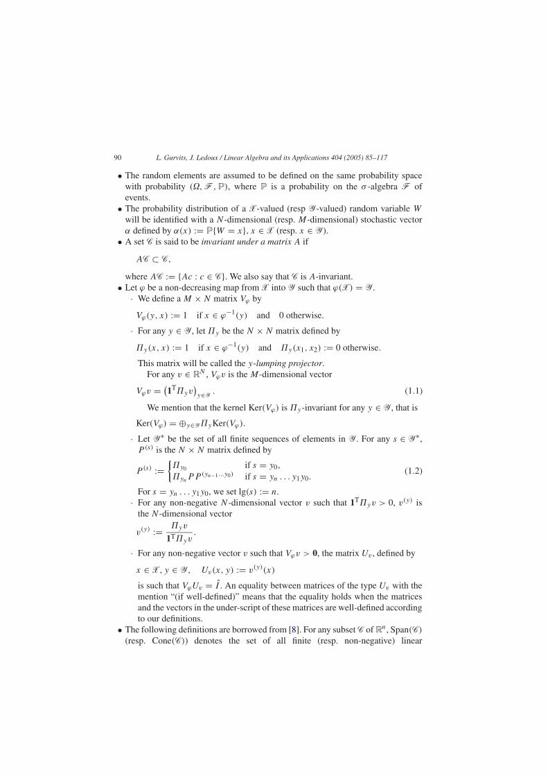
• The random elements are assumed to be defined on the same probability spacewith probability (�,F, P), where P is a probability on the σ -algebra F ofevents.

• The probability distribution of a X-valued (resp Y-valued) random variable W

will be identified with a N-dimensional (resp. M-dimensional) stochastic vectorα defined by α(x) := P{W = x}, x ∈ X (resp. x ∈ Y).

• A set C is said to be invariant under a matrix A if

AC ⊂ C,

where AC := {Ac : c ∈ C}. We also say that C is A-invariant.• Let ϕ be a non-decreasing map from X into Y such that ϕ(X) = Y.

· We define a M × N matrix Vϕ by

Vϕ(y, x) := 1 if x ∈ ϕ−1(y) and 0 otherwise.

· For any y ∈ Y, let �y be the N × N matrix defined by

�y(x, x) := 1 if x ∈ ϕ−1(y) and �y(x1, x2) := 0 otherwise.

This matrix will be called the y-lumping projector.For any v ∈ RN , Vϕv is the M-dimensional vector

Vϕv = (1T�yv

)y∈Y . (1.1)

We mention that the kernel Ker(Vϕ) is �y-invariant for any y ∈ Y, that is

Ker(Vϕ) = ⊕y∈Y�yKer(Vϕ).

· Let Y∗ be the set of all finite sequences of elements in Y. For any s ∈ Y∗,P (s) is the N × N matrix defined by

P (s) :={�y0 if s = y0,

�ynPP (yn−1...y0) if s = yn . . . y1y0.(1.2)

For s = yn . . . y1y0, we set lg(s) := n.· For any non-negative N-dimensional vector v such that 1T�yv > 0, v(y) is

the N-dimensional vector

v(y) := �yv

1T�yv.

· For any non-negative vector v such that Vϕv > 0, the matrix Uv , defined by

x ∈ X, y ∈ Y, Uv(x, y) := v(y)(x)

is such that VϕUv = I . An equality between matrices of the type Uv with themention “(if well-defined)” means that the equality holds when the matricesand the vectors in the under-script of these matrices are well-defined accordingto our definitions.

• The following definitions are borrowed from [8]. For any subset C of Rn, Span(C)

(resp. Cone(C)) denotes the set of all finite (resp. non-negative) linear


combinations of the elements of C. If C is a set of non-negative vectors, thenSpan(C) = Cone(C) − Cone(C). If Cone(C) = C then C is called a cone. If Cis a finite set, then Cone(C) is called a polyhedral cone. Any polyhedral cone Cof Rn has the form C = {v ∈ Rn : Hv � 0} where H ∈ Rm×n. This is a closedconvex subset of Rn.The cone C is said to be decomposable if C = C1 + C2, where C1 and C2 are twosub-cones of C such that Span(C1) ∩ Span(C2) = {0}. We write C = C1 ⊕ C2.Our basic instance of a decomposable cone is the cone denoted by CC(α, �., P )

for a fixed N-dimensional stochastic vector α. It is defined as the smallest sub-cone of RN+ that contains the vector α and that is invariant under the matrix P andthe lumping projectors �y , y ∈ Y. It is easily seen that

CC(α, �., P ) := Cone(P (s)α, s ∈ Y∗) . (1.3)

The basic properties of this cone are from its definition

y ∈ Y, �yCC(α, �., P ) ⊂ CC(α, �., P )

⇐⇒ CC(α, �., P ) = ⊕y∈Y�yCC(α, �., P )

PCC(α, �., P ) ⊂ CC(α, �., P ).

• For a N-dimensional stochastic vector α, the central linear subspace used in thispaper, is the linear hull CS(α, �., P ) of cone CC(α, �., P ) defined above. Thatis

CS(α, �., P ) := CC(α, �., P ) − CC(α, �., P )

= Span(P (s)α, s ∈ Y∗) . (1.4)

The subspace CS(α, �., P ) is the minimal subspace that contains α and that isinvariant under P and the lumping projectors �y , y ∈ Y. In particular, it satisfies

y ∈ Y, �yCS(α, �., P ) ⊂ CS(α, �., P )

⇐⇒ CS(α, �., P ) = ⊕y∈Y�yCS(α, �., P )

PCS(α, �., P ) ⊂ CS(α, �., P ).

2. Markov property for a function of an HMC

The Markov chains are the basic stochastic processes considered in this paper. Werecall the definition of a kth-order Markov chain. For k = 1, the process is simplysaid to be a homogeneous Markov chain.


Definition 1. Let E be a finite set. A sequence of E-valued random variables (Zn)

is said to be a homogeneous kth-order Markov chain (kth-HMC) with the transitionmatrix Q iff for any n � 0, (z, zn+k−1, . . . , z0) ∈ En+k+1,

P{Zn+k = z | Zn+k−1 = zn+k−1, . . . , Zn = zn, . . . , Z0 = z0}=Q(z, zn+k−1, . . . , zn) if P{Zn+k−1 =zn+k−1, . . . , Z0 = z0} > 0.

The set E is called the state space of (Zn). Note that∑

z∈E Q(z, zn+k−1, . . . , zn) =1. The probability distribution of Z0 is called the initial distribution of the process(Zn).

Let (Xn)n be an HMC with state space X. In Section 2, the N × N matrix P andthe N-dimensional stochastic vector α will stand for the transition matrix and theinitial distribution of the Markov chain (Xn) respectively. Let ϕ be a non-decreasingmap of X onto Y such that

ϕ(X) = Y, M < N.

Such a map defines a partition of X into the M classes (ϕ−1(y), y ∈ Y) and

ϕ(Xn) = y ⇐⇒ Xn ∈ ϕ−1(y).

The function ϕ will be called a lumping map. The process (ϕ(Xn)) will called thelumped process associated with (Xn)n. Considering the string s := yn . . . y1y0 ∈ Y∗means that we are interested in the successive visited mega-states y0, . . . , yn by thelumped model. The integer lg(s) corresponds to the number of transitions in the pathy0, . . . , yn. Note that with (1.2)

P{ϕ(Xn) = yn, . . . , ϕ(X0) = y0}= 1T�ynP�yn−1 · · ·�y1P�y0α = 1TP (s)α. (2.1)

2.1. Homogeneous kth-order Markov property

The following theorem provides a first criterion for (ϕ(Xn)) to be a kth-HMC.This criterion is in terms of the cone CC(α, �., P ) defined in (1.3).

Theorem 2. The process (ϕ(Xn)) is a kth-HMC with transition matrix P iff

CC(α, �., P ) ⊂ Ck(P ),

where

Ck(P ) :={β � 0 : ∀(yk−1, . . . , y0) ∈ Y,[

VϕP − Pyk−1,...,y01T]P (yk−1···y0)β = 0

}(2.2)

and Pyk−1,...,y0 denotes the vector(P (y, yk−1, . . . , y0)

)y∈Y .


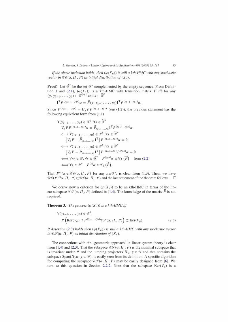
If the above inclusion holds, then (ϕ(Xn)) is still a kth-HMC with any stochasticvector in CC(α, �., P ) as initial distribution of (Xn).

Proof. Let Y∗

be the set Y∗ complemented by the empty sequence. From Defini-tion 1 and (2.1), (ϕ(Xn)) is a kth-HMC with transition matrix P iff for any(y, yk−1, . . . , y0) ∈ Yk+1 and s ∈ Y

∗

1TP (yyk−1...y0s)α = P (y; yk−1, . . . , y0)1TP (yk−1...y0s)α.

Since P (yyk−1...y0s) = �yPP (yk−1...y0s) (see (1.2)), the previous statement has thefollowing equivalent form from (1.1)

∀(yk−1, . . . , y0) ∈ Yk, ∀s ∈ Y∗

VϕPP (yk−1...y0s)α = Pyk−1,...,y01TP (yk−1...y0s)α

⇐⇒ ∀(yk−1, . . . , y0) ∈ Yk, ∀s ∈ Y∗[

VϕP − Pyk−1,...,y01T]P (yk−1...y0s)α = 0

⇐⇒ ∀(yk−1, . . . , y0) ∈ Yk, ∀s ∈ Y∗[

VϕP − Pyk−1,...,y01T]P (yk−1...y0)P (y0s)α = 0

⇐⇒ ∀y0 ∈ Y, ∀s ∈ Y∗

P (y0s)α ∈ Ck

(P

)from (2.2)

⇐⇒ ∀s ∈ Y∗ P (s)α ∈ Ck

(P

).

That P (s)α ∈ CC(α, �., P ) for any s ∈Y∗, is clear from (1.3). Then, we haveCC(P (s)α, �., P )⊂CC(α, �., P ) and the last statement of the theorem follows. �

We derive now a criterion for (ϕ(Xn)) to be an kth-HMC in terms of the lin-ear subspace CS(α, �., P ) defined in (1.4). The knowledge of the matrix P is notrequired.

Theorem 3. The process (ϕ(Xn)) is a kth-HMC iff

∀(yk−1, . . . , y0) ∈ Yk,

P(

Ker(Vϕ) ∩ P (yk−1...y0)CS(α, �., P ))

⊂ Ker(Vϕ). (2.3)

If Assertion (2.3) holds then (ϕ(Xn)) is still a kth-HMC with any stochastic vectorin CS(α, �., P ) as initial distribution of (Xn).

The connections with the “geometric approach” in linear system theory is clearfrom (1.4) and (2.3). That the subspace CS(α, �., P ) is the minimal subspace thatis invariant under P and the lumping projectors �y , y ∈ Y and that contains thesubspace Span(�yα, y ∈ Y), is easily seen from its definition. A specific algorithmfor computing the subspace CS(α, �., P ) may be easily designed from [6]. Weturn to this question in Section 2.2.2. Note that the subspace Ker(Vϕ) is a


(P, P (yk−1...y0)CS(α, �., P ))-conditioned invariant according to the terminologyused by Basile and Marro [6]. This last fact is not useful for our purpose.

Proof. Let (ϕ(Xn)) be a kth-HMC with some transition matrix P . We know fromTheorem 2 that CC(α, �., P ) ⊂ Ck(P ). Any vector v ∈ P (yk−1...y0)CS(α, �., P )

has the form P (yk−1...y0)(β − γ ) with β, γ ∈ Ck(P ). If v ∈ Ker(Vϕ) then

VϕPv=VϕPP (yk−1...y0)(β − γ )

= Pyk−1,...,y01TP (yk−1...y0)(β − γ ) since β, γ ∈ Ck(P )

= Pyk−1,...,y01Tv = 0 since 1Tv = 0.

Thus, the vector Pv is in Ker(Vϕ).Assume we have the inclusion in (2.3). In a first step, we define the matrix P

as follows. For any (yk−1, . . . , y0) ∈ Yk such that P (yk−1...y0)CC(α, �., P ) /= {0},select a non-trivial vector β in this set and put

Pyk−1...y0 := VϕPβ(yk−1). (2.4)

When P (yk−1...y0)CC(α, �., P ) = {0}, it is easily seen that, with P-probability 1, thepath yk−1 . . . y0 is not observable for (ϕ(Xn)). Then, the stochastic vector Pyk−1...y0

may be arbitrary chosen.In a second step, we have to prove that CC(α, �., P ) ⊂ Ck(P ). If

CC(α, �., P ) = {0} then this is trivially true. When CC(α, �., P ) /= {0}, let γ bea non-trivial vector of CC(α, �., P ). We must find that[

VϕP − Pyk−1,...,y01T]P (yk−1···y0)γ = 0. (2.5)

If P (yk−1...y0)γ = 0, this is obvious. If P (yk−1...y0)γ /= 0, then Eq. (2.5) has the fol-lowing equivalent form from (2.4)

VϕP(P (yk−1...y0)γ

)(yk−1) = Pyk−1...y0 = VϕPβ(yk−1).

Since(P (yk−1...y0)γ

)(yk−1) − β(yk−1) ∈ Ker(Vϕ), we have(P (yk−1...y0)γ

)(yk−1) −β(yk−1) ∈ Ker(Vϕ) ∩ P (yk−1...y0)CS(α, �., P ). We find from the inclusion (2.3) that

0 = VϕP

[(P (yk−1...y0)γ

)(yk−1) − β(yk−1)

]⇐⇒ VϕP

(P (yk−1...y0)γ

)(yk−1) = VϕPβ(yk−1). �

Corollary 4. Suppose the matrix (P (x1, x2))x1,x2∈ϕ−1(y) is non-singular for everyy ∈ Y. If (ϕ(Xn)) is an kth-HMC for some k � 2 then (ϕ(Xn)) is an HMC.

Proof. If (P (x1, x2))x1,x2∈ϕ−1(y) is a non-singular matrix then

∀Z ⊂ RN, ∀y ∈ Y, P (y...y)Z = P (yy)Z = �yZ.


If (ϕ(Xn)) is a kth-HMC, then we deduce from (2.3) with yk−1 . . . y0 := y . . . y andthe equality above, that

∀y ∈ Y, P(Ker(Vϕ) ∩ �yCS(α, �., P )

) ⊂ Ker(Vϕ).

Thus, (ϕ(Xn)) is a 1st-HMC from Theorem 3. �

We mention for completeness, the following spectral properties resulting fromthe kth-order lumpability property. They hold because the cone CC(α, �., P ) isinvariant under the matrices P and �yP�y , y ∈ Y (see [27, Lemma 3.3]). Whena probabilistic approach is favored, these properties combined with the additionalassumption of the existence of an “ergodic” type theorem, allow the derivation ofresults on (1-order) lumpability through limit arguments (e.g. see [24,35]).

Corollary 5

(1) If (ϕ(Xn)) is a kth-HMC, then it is still a kth-HMC with some stochastic eigen-vector of P as initial distribution of (Xn).

(2) If α is such that �yα /= 0 and (ϕ(Xn)) is a kth-HMC, then (ϕ(Xn)) is stilla kth-HMC with some stochastic eigenvector of �yP�y as initial distributionof (Xn).

Comment 1. If P is irreducible then the Perron–Frobenius theorem asserts thatthere exists an unique stochastic eigenvector π corresponding to the eigenvalue 1.This vector is the stationary distribution of the HMC (Xn). Let distr(X0) denotes theprobability distribution of X0. Then, we can write

(ϕ(Xn)) is a kth-HMC(with transition matrix P

)for distr(X0) := α

⇒ (ϕ(Xn)) is a kth-HMC(with transition matrix P

)for distr(X0) := π

⇒ (ϕ(Xn)) is a kth-HMC(with transition matrix P

)for distr(X0) ∈ Cπ

with Cπ := ⊕y∈YCone(�yπ)

since CC(u, �., P ) = CC(π, �., P ) for any u ∈ Cπ .

Let Z be any set of N-dimensional stochastic vectors. The linear subspaceCS(Z, �., P ) is defined from (1.4) by replacing the single vector α by the collec-tion of vectors Z. In other words, CS(Z, �., P ) is the minimal subspace includingZ that is invariant under P and �y, y ∈ Y. The reader will note that for the notationsto be consistent, CS(α, �., P ) should be interpreted as CS({α}, �., P ). We chooseto drop the braces in case of a single vector to lighten the notations.

The following result may be proved as Theorem 3 (the details are omitted).

Theorem 6. Let Z be a set of N-dimensional stochastic vectors. (ϕ(Xn)) is a kth-HMC for every α ∈ Z with a transition matrix that does not depend on α iff


∀(yk−1, . . . , y0) ∈ Yk,

P(

Ker(Vϕ) ∩ P (yk−1...y0)CS(Z, �., P ))

⊂ Ker(Vϕ). (2.6)

Note that the previous result is not valid if the transition matrix of (ϕ(Xn)) isallowed to depend on the probability distribution of X0 selected in Z.

2.2. Homogeneous Markov property

This subsection is devoted to the homogeneous (1st-order) Markov property ofthe lumped process (ϕ(Xn)).

Definition 7. If the process (ϕ(Xn)), is an HMC with transition matrix P , then theMarkov chain (Xn), or its transition matrix P , are said to be weakly lumpable withthe matrix P (w.r.t. the lumping map ϕ).

It is easily seen that (ϕ(Xn)) may be an HMC with a transition matrix whichdepend on α. However, it follows from Corollary 5, that this transition matrix onlydepends on P and the map ϕ for a broad class of Markov chains (e.g. see Comment 1[28]).

2.2.1. Local characterizationThe cone C1(P ) is from (2.2)

C1(P ) = {β � 0 : ∀y ∈ Y,

[VϕP − P Vϕ

]�yβ = 0

}. (2.7)

Specializing Theorem 2 for k = 1, we get the following criterion of weak lumpabil-ity.

Corollary 8. The process (ϕ(Xn)) is an HMC with transition matrix P iff

CC(α, �., P ) ⊂ C1(P ).

If the above inclusion holds, then (ϕ(Xn)) is still an HMC with the transition matrixP for any stochastic vector in CC(α, �., P ) as initial distribution of (Xn).

A new sufficient condition for weak lumpability. Let us check that a sufficient condi-tion for weak lumpability is given by

∀y ∈ Y, PUα = PUPα(y) (if well-defined). (2.8)

This relation is equivalent to

∀y0, y1, y2, �y2P�y1P�y0α ∝ �y2P�y1α.


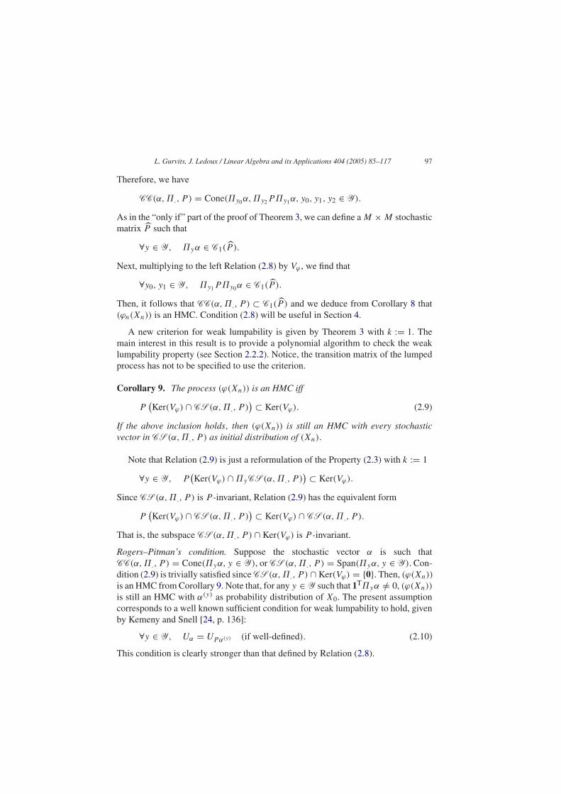
Therefore, we have

CC(α, �., P ) = Cone(�y0α, �y2P�y1α, y0, y1, y2 ∈ Y).

As in the “only if” part of the proof of Theorem 3, we can define a M × M stochasticmatrix P such that

∀y ∈ Y, �yα ∈ C1(P ).

Next, multiplying to the left Relation (2.8) by Vϕ , we find that

∀y0, y1 ∈ Y, �y1P�y0α ∈ C1(P ).

Then, it follows that CC(α, �., P ) ⊂ C1(P ) and we deduce from Corollary 8 that(ϕn(Xn)) is an HMC. Condition (2.8) will be useful in Section 4.

A new criterion for weak lumpability is given by Theorem 3 with k := 1. Themain interest in this result is to provide a polynomial algorithm to check the weaklumpability property (see Section 2.2.2). Notice, the transition matrix of the lumpedprocess has not to be specified to use the criterion.

Corollary 9. The process (ϕ(Xn)) is an HMC iff

P(Ker(Vϕ) ∩ CS(α, �., P )

) ⊂ Ker(Vϕ). (2.9)

If the above inclusion holds, then (ϕ(Xn)) is still an HMC with every stochasticvector in CS(α, �., P ) as initial distribution of (Xn).

Note that Relation (2.9) is just a reformulation of the Property (2.3) with k := 1

∀y ∈ Y, P(Ker(Vϕ) ∩ �yCS(α, �., P )

) ⊂ Ker(Vϕ).

Since CS(α, �., P ) is P -invariant, Relation (2.9) has the equivalent form

P(Ker(Vϕ) ∩ CS(α, �., P )

) ⊂ Ker(Vϕ) ∩ CS(α, �., P ).

That is, the subspace CS(α, �., P ) ∩ Ker(Vϕ) is P -invariant.

Rogers–Pitman’s condition. Suppose the stochastic vector α is such thatCC(α, �., P ) = Cone(�yα, y ∈ Y), or CS(α, �., P ) = Span(�yα, y ∈ Y). Con-dition (2.9) is trivially satisfied since CS(α, �., P ) ∩ Ker(Vϕ) = {0}. Then, (ϕ(Xn))

is an HMC from Corollary 9. Note that, for any y ∈ Y such that 1T�yα /= 0, (ϕ(Xn))

is still an HMC with α(y) as probability distribution of X0. The present assumptioncorresponds to a well known sufficient condition for weak lumpability to hold, givenby Kemeny and Snell [24, p. 136]:

∀y ∈ Y, Uα = UPα(y) (if well-defined). (2.10)

This condition is clearly stronger than that defined by Relation (2.8).


The matrix-condition (2.10) has been generalized for the class of HMCs with ageneral state space by Rogers and Pitman [33]. It is based on the following specificcondition satisfied by the transition matrix.

Definition 10. A stochastic matrix P is called a R–P matrix if there exist a N × M

stochastic matrix � such that

Vϕ� = I and P� = �VϕP�. (2.11)

We mention an interesting property of a Markov chain (Xn) with a R–P transitionmatrix P . The probability distributions of random variables Xn, n = 1, . . . may becomputed as follows. We deduce from Relation (2.11) that

P n� = �(VϕP�)n, ∀n � 1.

Thus, with any stochastic vector in the cone �RM+ as probability distribution of X0,the one-dimensional distributions of the Markov chain (Xn) can be computed fromthe M × M matrix VϕP�. When � = U1, such a fact is known from [14] and isused in [38,10]. This was one of the main motivations to deal with R–P matrices forinvestigating Markov bounds for functions of an HMC in [29].

Specializing Theorem 6 for k = 1, we obtain the following statement.

Corollary 11. Let Z be a subset of probability distributions on X. (ϕ(Xn)) is anHMC for every α ∈ Z with a transition matrix that does not depend on α iff

P(Ker(Vϕ) ∩ CS(Z, �., P )

) ⊂ Ker(Vϕ). (2.12)

Strong lumpability. When Z is the set of all the probability distributions over Xin Corollary 11, we obtain the so-called lumpability property or strong lumpabil-ity property of the transition matrix P . This property is widely used in stochasticmodeling because it can be easily checked on the transition matrix or on the associ-ated graph (e.g. see [38,19,9]). Since Z is assumed to be the set of N-dimensionalstochastic vectors, we have Span(Z) = RN . Since Z ⊂ CS(Z, �., P ) by defini-tion, it follows that CS(Z, �., P ) = RN . Then, Relation (2.12) gives the followingcriterion for strong lumpability:

P Ker(Vϕ) ⊂ Ker(Vϕ). (2.13)

We can take P := VϕPU1 as the transition matrix of (ϕ(Xn)).

In fact, the following criteria for strong lumpability may be easily derived [24,6,12].

Theorem 12. Let P be a stochastic matrix and P be the matrix VϕPU1. The fol-lowing statements are equivalent.


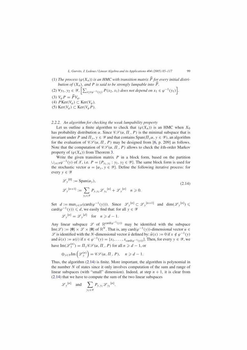
(1) The process (ϕ(Xn)) is an HMC with transition matrix P for every initial distri-bution of (Xn), and P is said to be strongly lumpable into P .

(2) ∀y1, y2 ∈ Y,[∑

x2∈ϕ−1(y2)P (x2, x1) does not depend on x1 ∈ ϕ−1(y1)

].

(3) VϕP = P Vϕ .(4) P Ker(Vϕ) ⊂ Ker(Vϕ).(5) Ker(Vϕ) ⊂ Ker(VϕP ).

2.2.2. An algorithm for checking the weak lumpability propertyLet us outline a finite algorithm to check that (ϕ(Xn)) is an HMC when X0

has probability distribution α. Since CS(α, �., P ) is the minimal subspace that isinvariant under P and �y , y ∈ Y and that contains Span(�yα, y ∈ Y), an algorithmfor the evaluation of CS(α, �., P ) may be designed from [6, p. 209] as follows.Note that the computation of CS(α, �., P ) allows to check the kth-order Markovproperty of (ϕ(Xn)) from Theorem 3.

Write the given transition matrix P in a block form, based on the partition∪y∈Yϕ−1(y) of X, i.e. P = {Py1,y2 : y1, y2 ∈ Y}. The same block form is used forthe stochastic vector α = {αy, y ∈ Y}. Define the following iterative process: forevery y ∈ Y

Ly[0] := Span(αy), (2.14)

Ly[n+1] :=

∑y1∈Y

Py,y1Ly1[n] + Ly

[n] n � 0.

Set d := maxy∈Y(card(ϕ−1(y))). Since Ly[n] ⊂ Ly

[n+1] and dim(Ly[n]) �

card(ϕ−1(y)) � d , we easily find that: for all y ∈ Y

Ly[n] = Ly

[d] for n � d − 1.

Any linear subspace L of Rcard(ϕ−1(y)) may be identified with the subspaceIm(L) := {0} × L × {0} of RN . That is, any card(ϕ−1(y))-dimensional vector u ∈L is identified with the N-dimensional vector u defined by: u(x) := 0 if x /∈ ϕ−1(y)

and u(x) := u(i) if x ∈ ϕ−1(y) = {x1, . . . , xcard(ϕ−1(y))}. Then, for every y ∈ Y, we

have Im(L(n)y ) = �yCS(α, �., P ) for all n � d − 1, or

⊕y∈YIm(L(n)

y

)= CS(α, �., P ), n � d − 1.

Thus, the algorithm (2.14) is finite. More important, the algorithm is polynomial inthe number N of states since it only involves computation of the sum and range oflinear subspaces (with “small” dimension). Indeed, at step n + 1, it is clear from(2.14) that we have to compute the sum of the two linear subspaces

Ly[n] and

∑y1∈Y

Py,y1Ly1[n].


Suppose that a basis of Ly1[n] for y1 ∈ Y is given. The main computational task

is the computation of the M < N ranges Py,y1Ly1[n]. Such computations may be

performed with the Gaussian elimination procedure which is known to be polynomialin the dimensions and bit-sizes involved (e.g. [17, p. 112]).

In the same way, we get a polynomial-time algorithm to construct CS(Z, �., P ),where Z is a set of N-dimensional stochastic vectors, provided that theminimal linear subspace containing Z has “effective” representation. Clearly, inthis case, we also can check in polynomial-time the weak lumpability property withrespect to the set of initial distributions Z. We will use this observation inSection 4.

The next result follows from Definition 1, (2.1) and (1.4).

Proposition 13. The homogeneous Markov property of (ϕ(Xn)) is checked fromk � maxy∈Y(card(ϕ−1(y))) steps of the algorithm above.

Rosenblatt’s algorithm to check the weak lumpability is based on Corollary 8, whichis essentially the criterion of weak lumpability given by Kemeny and Snell [24] foran irreducible matrix P (see also [35, Theorem 3.4]). Proposition 13 shows that thecone CC(α, �., P ) may be computed in at most maxy∈Y(card(ϕ−1(y))) steps. Thus,Rosenblatt’s algorithm is finite. However, the extremal rays of cones are needed forthese algorithms and their computation is exponential in the dimensions involved.Rosenblatt’s algorithm is essentially a Bayesian computation and is “mildly” nonlin-ear. The main contribution of the algorithm associated with (2.14) is to show that itis possible to avoid the “Bayesian” nonlinearity.

Comment 2. In this paper, we only deal with discrete-time Markov chains. Themain criteria for a function of a discrete-time Markov chain to be an HMC carryover in the continuous-time context. Indeed, the “uniformization procedure”, whichis a basic tool for the numerical analysis of continuous time Markov models [41],may be used to derive from a continuous-time Markov chain (Xt )t∈R+ , a discrete-time Markov chain to which our results apply. This discrete-time Markov chainis called the “uniformized” chain associated with (Xt )t∈R+ . The following resultmay be proved (see [22] for further details). For a Markov process (Xt )t∈R+ anda lumping map ϕ, checking that the process (ϕ(Xt ))t∈R+ is an HMC with afixed probability distribution of X0, consists in applying the algorithm ofSection 2.2.2 to the uniformized chain associated with (Xt )t∈R+ Under specificassumptions on the continuous time Markov chain (Xt )t∈R+ , this property is knownfrom [36,26].

2.2.3. Global characterizationMany papers are concerned with the derivation of the set DM(P ) of all probability

distributions of X0 such that (ϕ(Xn)) is an HMC with the transition matrix P (e.g.


see [35,27] and the references therein). From Corollary 8, this set is the collection ofall stochastic vectors in

CM(P ) :={α ∈ RN+ : CC(α, �., P ) ⊂ C1(P )

}. (2.15)

The following properties of the set CM(P ) are easily seen from its definition:

(P1) CM(P ) is a closed convex cone.(P2) CM(P ) is invariant under the matrix P and the lumping projectors �y , y ∈ Y.(P3) CM(P ) is the maximal sub-cone of C1(P ) that is invariant under all lumping

projectors and matrix P . In other words, DM(P ) is the maximal subset Z ofthe set of all probability distributions over X, such that P(CS(Z, �., P ) ∩Ker(Vϕ)) ⊂ Ker(Vϕ).

(P4) If �yCM(P ) = {0} then, with P-probability 1, the state class ϕ−1(y) can neverbe accessed by the Markov chain (Xn) with any initial distribution in CM(P ).

Property (P4) leads us to define the notion of essentially weakly lumpable matrix.

Definition 14. The Markov chain (Xn), or its transition matrix P , are said to beessentially weakly lumpable with the matrix P if (∀y ∈ Y, �yCM(P ) /= {0}).

Note that a weakly lumpable irreducible matrix P is essentially weakly lumpablefrom Comment 1.

Any vector α in CM(P ) is a solution of the linear equations{0 = [

VϕP − P Vϕ

]P (s), s ∈ Y∗} (see Corollary 8). When CM(P ) is non-trivial,

it is clear from Proposition 13 that,

CM(P ) =maxy∈Y(card(ϕ−1(y)))−1⋂

k=0

{v ∈ RN

+ : ∀s ∈ Y∗, lg(s) � k,

[VϕP − P Vϕ

]P (s)v = 0

}.

Therefore, the cone CM(P ) has the central property to be polyhedral. Next, the fol-lowing criterion of weak lumpability is easily derived from [27, Theorem 3.4].

Theorem 15. CM(P ) /= {0} iff there exist a non-negative K × K matrix Q and anon-negative N × K matrix U (1 � K � N) such that

Cone(U) ⊂ C1(P ), Cone(U) = ⊕y∈Y�yCone(U), PU = UQ (2.16)

with Cone(U) := URM+ and dimCone(U) = K. In such a case, Cone(U) ⊂ CM(P ).

For a R–P matrix P , Conditions (2.11) have to be compared to Conditions (2.16).Indeed, the matrices U , P and Q in (2.16) may be identified with �, Q = P =VϕP� in (2.11) respectively. We see from (2.16) that Cone(�) := �RM+ is invari-

ant under P and the lumping projectors. We have that Cone(�) ⊂ CM(P ) and P isessentially weakly lumpable. But the set CM(P ) may be larger than Cone(�).


Let us denote the spectrum of a matrix A by σ(A). The following spectral prop-erties arise from the weak lumpability property and can be proved from [5,27].

Corollary 16. If P is essentially weakly lumpable with matrix P , then we have

∀y ∈ Y, P (y, y) ∈ σ(�yP�y) and σ(P ) ⊂ σ(P ).

2.2.4. Duality resultsIn this subsection, the Markov chain (Xn) and its dual version w.r.t. the scalar

product defined in (2.17) are considered. The Markov property of their respectivelumped processes is examined. Our results generalize the Theorems 6.4.5 and 6.4.8in [24], where the transition matrix P is assumed to be primitive (that is irreducibleand aperiodic). Note that the method of derivation is new.

Let v be a positive vector of RN . The N × N diagonal matrix with generic diag-onal entry v(i) is denoted by diag(v). We define a scalar product 〈·, ·〉v on RN by

∀x, y ∈ RN, 〈x, y〉v := xTdiag(v)−1y. (2.17)

Definition 17. Let P be a N × N stochastic matrix. The adjoint matrix P ∗ of P

w.r.t. the scalar product 〈·, ·〉v is defined by

P ∗ := diag(v)P Tdiag(v)−1.

We have (P ∗)∗ = P .

The matrix P ∗ is stochastic if and only if the vector v is an eigenvector corre-sponding to the eigenvalue 1 of P . If P ∗ is stochastic, then P ∗ is the well knowndual or time-reversed matrix of P [24, Definition 3.5.1]. When P ∗ = P , the matrixP is said to be self-adjoint, or reversible in the Markov chain framework. A selfadjoint matrix P is an instance of a normal matrix, that is, P satisfies PP ∗ = P ∗P .

Let H be a linear subspace of RN . The space RN is the direct sum

RN = H ⊕ H∗, (2.18)

where H∗ := {w ∈ RN : 〈w, h〉v = 0, h ∈ H

}is the adjoint subspace of H. Note

that (H∗)∗ = H and we know that

PH ⊂ H ⇐⇒ P ∗H∗ ⊂ H∗. (2.19)

If P is a normal matrix, then we have [16, p. 275]

PH ⊂ H ⇐⇒ PH∗ ⊂ H∗. (2.20)

Theorem 18. Let v be a positive stochastic vector. We define the linear subspaceV := Span(v(y), y ∈ Y). Then,

(1) V is P -invariant if and only if Ker(Vϕ) is P ∗-invariant.


(2) When P is a normal matrix, we have

P(Ker(Vϕ) ∩ CS(v, �., P )

) ⊂ Ker(Vϕ)

⇐⇒ P Ker(Vϕ) ⊂ Ker(Vϕ) ⇐⇒ PV ⊂ V.

Proof. A direct computation shows that V∗ = Ker(Vϕ) and hence, V= (Ker(Vϕ))∗.Applying Relation (2.19) to H := V gives Statement (1). When the matrix P is nor-mal, the second equivalence in Statement (2) is just Relation (2.20) with H := V.Next, we have V ⊂ CS(v, �., P ) by definition of the last subspace. This inclusionhas the equivalent form

CS(v, �., P )∗ ⊂ V∗ = Ker(Vϕ).

Moreover, the subspace CS(v, �., P ) is P -invariant. The matrix P is assumed to benormal, so that CS(v, �., P )∗ is P -invariant from (2.20). Since CS(v, �., P )∗ ∩Ker(Vϕ) = CS(v, �., P )∗, we find that

P(Ker(Vϕ) ∩ CS(v, �., P )∗

) ⊂ Ker(Vϕ).

The first equivalence in Statement (2) is proved as follows. Suppose thatP(Ker(Vϕ) ∩ CS(v, �., P )) ⊂ Ker(Vϕ). Then, we deduce from (2.18) with H :=CS(v, �., P )∗ and from the inclusion above, that

P Ker(Vϕ) ⊂ Ker(Vϕ).

The converse statement easily follows from the P -invariance of CS(v, �., P ). �

When the matrix P ∗ is stochastic, the previous theorem reads as follows.

Corollary 19. Assume that P has a positive stochastic eigenvector v associatedwith its eigenvalue 1. Then

(1) P is a R–P matrix if and only if P ∗ is strongly lumpable.(2) When the matrix P is irreducible and normal, the three following statements

are equivalent: P is weakly lumpable; P is strongly lumpable; P is a R–Pmatrix.

Proof. This is just a reformulation of Theorem 18 once the following commentshave been mentioned. P is a R–P matrix with associated matrix � iff the cone �RM+is P -invariant, which is easily checked to be equivalent to the subspace �RM isP -invariant. Assuming P irreducible is equivalent to assuming that P has an uniquestochastic eigenvector associated with the eigenvalue 1 [8, p. 27]. We need thisassumption only to derive from Statement (1) in Corollary 5, that the inclusionP(Ker(Vϕ) ∩ CS(v, �., P )) ⊂ Ker(Vϕ) holds when (Xn) is weakly lumpable. �


2.3. Non-homogeneous Markov property

We are interested in a criterion for (ϕ(Xn)) to be a non-homogeneous Markovchain. A related problem was studied by Kelly [23] under the assumption that (Xn)

was a non-homogeneous Markov chain.

Definition 20. The process (ϕ(Xn)) is a non-homogeneous Markov chain (NHMC)with the transition matrices (Pn)n�0 iff for every n � 0 and for every (yn+1, . . . , y0) ∈Yn+2, we have

P{ϕ(Xn+1) = yn+1 | ϕ(Xn) = yn, . . . , ϕ(X0) = y0} = Pn(yn+1, yn)

if P{ϕ(Xn) = yn, . . . , ϕ(X0) = y0} > 0.

Proceeding as in the homogeneous case, we obtain that (ϕ(Xn)) is an NHMCwith the transition matrices (Pn)n�0 iff for any n � 0 and any (yn, . . . , y0) ∈ Yn+1[

VϕP − PnVϕ

]P (yn...y0)α. (2.21)

Let us define the following sub-cones of RN+ :

C(Pn

) := {β � 0 : ∀y ∈ Y,

[VϕP − PnVϕ

]β = 0

}, n � 0,

CC0(α) := ⊕y∈YCone(�yα),

CCn+1(α) := ⊕y∈Y�yPCCn, n � 0.

}(2.22)

Using the cones CCn(α) and Condition (2.21), the following criterion for (ϕ(Xn) tobe an NHMC may be derived as Theorem 2. The details are omitted.

Theorem 21. (ϕ(Xn)) is an NHMC with the transition matrices (Pn)n�0 iff

CCn(α) ⊂ C(Pn), ∀n � 0.

Assume the above inclusion holds and set the initial distribution of (Xn) toP (s)α/1TP (s)α for some s ∈ Y∗ with lg(s) = k. Then, (ϕ(Xn)) is an NHMC withthe transition matrices (Pn+k)n�0.

The last statement in Theorem 21 follows from the inclusion CCn(P(s)α) ⊂

CCn+k(α) for any s ∈ Y∗ such that lg(s) = k. Now, we find a criterion in termsof the linear spaces

CSn(α) := CCn(α) − CCn(α) n � 0,

which does not require the knowledge of matrices (Pn)n�0.

Theorem 22. The process (ϕ(Xn)) is an NHMC iff

∀n � 0, P(Ker(Vϕ) ∩ CSn(α)

) ⊂ Ker(Vϕ). (2.23)

Proof. The proof of the “only if” part is as in that of Theorem 3.


The converse statement is proved as follows. In a first step, we define the matrices(Pn)n�0 as follows. Let n � 0 be fixed. For any y ∈ Y such that �yCCn(α) /= {0},select a vector β in this set. We set

Pn(., y) := VϕPβ(y). (2.24)

When �yCCn(α) = {0}, (ϕ(Xn)) does not visit the state y at time n with P-probabil-ity 1. Then, the stochastic vector Pn(., y) may be arbitrary chosen. In a second step,we have to prove that �yCCn(α) ⊂ C(Pn) for every y ∈ Y. If �yCCn(α) = {0}then the inclusion is trivial. If not, we just have to justify that

∀γ ∈ �yCCn(α), VϕPγ (y) = Pn(., y) = VϕPβ(y) (from (2.24)).

Since γ (y) − β(y) ∈ Ker(Vϕ), we have γ (y) − β(y) ∈ CSn(α) ∩ Ker(Vϕ). It followsfrom the inclusion (2.23), that 0 = VϕP

(γ (y) − β(y)

)and VϕPγ (y) = VϕPβ(y). �

Example 23. Let us consider an HMC (Xn) with transition matrix P and the lump-ing map ϕ defined by

P =0 0 1

1 0 00 1 0

, ϕ(1) = 1, ϕ(2) = ϕ(3) = 2.

Take e1 = (1, 0, 0)T as initial distribution. Starting in state 1, the path of process(ϕ(Xn)) is 1, 2, 2, 1, 2, 2, . . . with P-probability 1. Therefore (ϕ(Xn)) is a Markovchain. The sequence of transitional matrices may be chosen as

Pn :=(

0 01 1

)if n ≡ 0 mod 3;

Pn :=(

1 00 1

)if n ≡ 1 mod 3;

Pn :=(

1 10 0

)if n ≡ 2 mod 3.

However, note that two entries of each matrix of the sequence are arbitrary. Indeed,a simple computation shows that

CCn(e1) = Cone(e1), Pn(., 1) = (0, 1)T if n ≡ 0 mod 3,

CCn(e1) = Cone(e2), Pn(., 2) = (0, 1)T if n ≡ 1 mod 3,

CCn(e1) = Cone(e3), Pn(., 1) = (1, 0)T if n ≡ 2 mod 3.

Since Ker(Vϕ) = Span((0, 1, −1)) and CSn(e1) ∩ Ker(Vϕ) = {0}, the criterion inTheorem 22 is satisfied.

A natural question is: can a lumped process (ϕ(Xn)) be an NHMC for everyprobability distribution of X0? The answer is “negative” if we require that all lumped


NHMC share the same sequence of transition matrices (Pn)n�0. In fact, the lumpedprocess will be actually a homogeneous Markov chain. Indeed, if (ϕ(Xn)) is anNHMC with transition matrices (Pn)n�0 for every initial distribution, we deducefrom Theorem 21 that C(P0) = RN+ and we have VϕP − P0Vϕ = 0. We recognize acondition for (Xn) to be strongly lumpable (see Theorem 12). Let ex be the xth vectorof the canonical basis of RN . It can be seen that (ϕ(Xn)) may be an NHMC for anyinitial distribution ex (x ∈ X) without being an NHMC for every initial distribution[22].

Now, we investigate the conditions under which (ϕ(Xn)) is an NHMC with aperiodic sequence of transition matrices (Pn)n�0. We just present a criterion for the2-periodic case. The general situation is quite similar. It is clear from Theorem 21that (ϕ(Xn)) is an NHMC with a 2-periodic sequence of transition matrices (Pn)n�0iff

∀n � 0, CC2n(α) ⊂ C(P0) and CC2n+1(α) ⊂ C(P1) (2.25)

or CCe(α) ⊂ C(P0) and CCo(α) ⊂ C(P1)

with CCe(α, �., P ) := ∑n�0 CC2n(α) and CCo(α, �., P ) := ∑

n�0 CC2n+1(α).Note that

PCCe(α, �., P ) ⊂ CCo(α, �., P ) and

PCCo(α, �., P ) ⊂ CCe(α, �., P ). (2.26)

In such a context, we obtain the following criterion for weak lumpability. The proofis similar to that of Theorem 22 and is omitted.

Theorem 24. The process (ϕ(Xn)) is a 2-periodic NHMC iff

P(Ker(Vϕ) ∩ CSe(α, �., P )

) ⊂ Ker(Vϕ) ∩ CSo(α, �., P ) and

P(Ker(Vϕ) ∩ CSo(α, �., P )

) ⊂ Ker(Vϕ) ∩ CSe(α, �., P )

where

CSe(α, �., P ) := CCe(α, �., P ) − CCe(α, �., P ) and

CSo(α, �., P ) := CCo(α, �., P ) − CCo(α, �., P ).

3. ϕ-Observability

In this section, the matrix P is the transition matrix of the Markov chain (Xn).The following linear system can be considered from matrices P and Vϕ

xn+1 := Pxn and yn := Vϕyn n � 0,


where the “state vector” xn corresponds to the probability distribution of the randomvariable Xn. The “observed vector” yn is the probability distribution of the randomvariable ϕ(Xn).

Let us recall that the pair of matrices (P, Vϕ) is said to be observable if the so-called non-observable space is reduced to {0}, that is (e.g. see [6])⋂

k∈N

Ker(VϕP k) = {0}.

In an intuitive sense, the pair (P, Vϕ) is observable if the initial state x0 (probabilitydistribution of X0) can be computed by suitable processing of the observed vectors(probability distributions of ϕ(Xn)). The observability concept above, is appropriatefor the study of the one-dimensional distributions of the lumped process (ϕ(Xn)). Itis clear from (2.1) that we need a concept of observability adapted to the study offinite-dimensional distributions (or paths) of the lumped process. Such a concept hasbeen introduced by Gurvits for the investigation of the stability of linear inclusions[21] (see also [20]) and by Amari and co-authors [3] in the context of identifiabilityof hidden Markov models [3].

Let us define the non-ϕ-observable space by

NOP,ϕ :={v ∈ RN : ∀s ∈ Y∗, VϕP (s)v = 0

}. (3.1)

It is easily checked that NOP,ϕ is the maximal subspace of Ker(Vϕ) that is invariantunder all lumping projectors and the matrix P . The finite generation of this subspaceis similar to that of the non-observable space in linear system theory (e.g. see [6,Section 3]).

Definition 25. A pair of matrices (P, Vϕ) is said to be ϕ-observable if

NOP,ϕ = {0}.

In an intuitive sense, the pair (P, Vϕ) is ϕ-observable if the probability distri-bution of X0 can be computed from the knowledge of the finite-dimensional distri-butions of (ϕ(Xn)) [22]. That any observable pair (P, Vϕ) is ϕ-observable, is clearfrom their respective interpretations.

3.1. Connection between the sets CM (P ) and NOP,ϕ

The decomposable coneCM(P ) defined in (2.15) is connected to the spaceNOP,ϕ

as follows. Let α(1)y and α

(2)y be two stochastic vectors in �yCM(P ). Consider the

two Markov chains with the same transition matrix P and respective initial distri-butions α

(1)y and α

(2)y . They give rise to the same lumped process, which is an HMC

with the transition matrix P and the initial distribution Vϕα(1)y = Vϕα

(2)y = ey , where


ey is the yth vector of the canonical basis of RM . Then, it follows from (2.1) (1.1)

and (3.1) that α(1)y − α

(2)y ∈ NOP,ϕ . Noting that the set NOP,ϕ is the direct sum

⊕y∈Y�yNOP,ϕ and that �y(NOP,ϕ) ∩ RN+ = {0}, the proof of the next result iseasily completed from [28, Theorem 3.2].

Theorem 26. Suppose the cone �yCM(P ) in (2.15) contains a stochastic vectorαy. Then,

�yCM(P ) = [Span(αy) ⊕ �yNOP,ϕ] ∩ RN+ and

dim(�yCM(P )) = dim(�yNOP,ϕ) + 1,

where dim(�yCM(P )) is the dimension of the affine hull of the set �yCM(P ).

When P is essentially weakly lumpable, there exists a stochastic vector α suchthat

Vϕα > 0 and CM(P ) = [NOP,ϕ ⊕ Span(�yα, y ∈ Y)] ∩ RN+ .

When the pair (P, Vϕ) is ϕ-observable, we obtain the following criterion for theHMC (Xn) to be essentially weakly lumpable.

Corollary 27. Let P be a M × M stochastic matrix. If the pair (P, Vϕ) is ϕ-obser-vable (observable) then the following statements are equivalent.

(1) P is essentially weakly lumpable with matrix P .

(2) CM(P ) = �RN+ for some stochastic matrix � such that Vϕ� = I .

(3) P is a R–P matrix.

Proof. Assume that NOP,ϕ = {0}. If P is weakly lumpable with P then it fol-lows from Theorem 26 that CM(P ) = �RM+ with �ey = α(y) for any y ∈ Y andVϕ� = I . Property (P3) (p. 101) and Theorem 15 give that P� = �Q for somenon-negative matrix Q. In other words, P is a R–P matrix. The fact that Statement(3) implies Statement (1) is already known (see pages 98 and 101). �

3.2. Nowhere density of the set of weakly lumpable matrices

Let M be the linear space of real N × N matrices and S be the set of stochastic

matrices. A subset H of S is said to be nowhere dense in S, ifo

H = ∅ where H ando

H are respectively the closure and the interior of H in S. Note that a closed subsetH of S is nowhere dense in S if its complement set Hc is dense in S. It is clearthat a finite union of nowhere dense closed subsets of S is also nowhere dense in S.


The two following lemmas are easily proved from [16, p. 62] and [40, Proposition3.3.12] respectively.

Lemma 28. The set of all positive stochastic matrices is an open subset of S, whichis dense in S.

Lemma 29. Let us fix the lumping map ϕ. The set Eϕ := {P ∈ S : (Vϕ, P ) is notobservable} is a closed subset of S that is nowhere dense in S.

Lemma 30. Let us fix the lumping map ϕ. The set RPϕ of the R–P matrices is aclosed subset of S that is nowhere dense in S.

Proof. Let (Pn) be a sequence of elements in RPϕ converging to P . Since Pn ∈RPϕ , there exist stochastic matrices �n and Pn with Pn�n = �nPn. The sets ofstochastic matrices are compact, so we can extract subsequences (�nk

), (Pnk) from

(�n) and (Pn) that converge to some stochastic matrices � and P , respectively. Wehave

P� ←−k→+∞ Pnk

�nk= �nk

Pnk−→

k→+∞ �P

and P ∈ RPϕ .Let ey be the yth vector of the canonical basis of RM . Condition (2.10) for P to

be a R–P matrix may be reformulated as

∀y1, y0 ∈ Y, �y1P�y0�ey0 ∝ �ey1 .

We have to prove that the interior of RPϕ w.r.t. S is empty. In other words, if P ∈RPϕ then we must find a stochastic matrix Pε, as closed to P as necessary, such thatPε /∈ RPϕ . If 1 < M < N then there exists a class ϕ−1(y) with 2 � card(ϕ−1(y)) <

N . We only perturb the entries of P corresponding to the transition probabilities fromstates in ϕ−1(y0) to states in ϕ−1(y) for some y0 /= y to obtain Pε. Since we chooseIy1PIy1 = Iy1PεIy1 for all y1 ∈ Y, we just have to assert that the perturbations ofentries of �yP�y0 may be arbitrary small such that matrix Pε is stochastic andvector �yP�y0�ey0 is not proportional to �ey for some y0 /= y. It is clear that thiscan be done, so that Pε is not a R–P matrix. �

Corollary 27 is reformulated as follows.If P is essentially weakly lumpable w.r.t. the lumping map ϕ, then either the pair(Vϕ, P ) is not observable (not ϕ-observable) or the matrix P is a R–P matrix.

Now, we state the main result of this subsection.

Theorem 31. The set of all weakly lumpable matrices is nowhere dense in S.

Proof. Let us fix a lumping map ϕ from X. The set of all essentially weakly lum-pable matrices according to ϕ, denoted by EWLϕ , is such that

EWLϕ ⊂ RPϕ ∪ Eϕ.


We deduce from Lemmas 29 and 30 that RPϕ ∪ Eϕ is a closed and nowhere densesubset of S. Since X is assumed to be a finite set, the set of lumping maps from X isalso a finite set. Hence, the set of essentially weakly lumpable matrices is containedin the finite union ∪ϕ(RPϕ ∩ Eϕ) of closed and nowhere dense subsets. The proofis easily completed if we prove that the set of all non-essentially weakly lumpablematrices is also contained in a nowhere dense closed subset of S.

Note that the weak lumpability property for a positive stochastic matrix is equiva-lent to the essential weak lumpability property. Moreover, we deduce from Lemma 28,that the set of all non-positive matrices is closed and nowhere dense in S. Con-sequently, the set of all non-essentially weakly lumpable matrices is included in anowhere dense closed subset of S. �

4. Markov property for a probabilistic function of a Markov chain

4.1. Hidden Markov chains

Let us give an intuitive description of a hidden Markov chain. The mechanism ofsuch a model is as follows (e.g see [34] for further reading). We have a finite set of“states”, say X. At each clock time n, a new state is entered based upon a transitionprobability distribution which depends on the previous state (the Markov property).After each transition is made, an observation output symbol in Y is produced accord-ing to a probability distribution which depends on the current state. This probabilitydistribution is held fixed for the state regardless of when and how the state is entered.A formal definition of a hidden Markov chain is as follows.

Definition 32. A bivariate homogeneous Markov chain ((Yn, Xn)) with the statespace Y × X is said to be a hidden Markov chain, if its transition matrix Q satisfies

∀x, x1 ∈ X, ∀y, y1 ∈ Y, ∀n � 1

Q((y, x), (y1, x1)) = P{(Yn, Xn) = (y, x) | (Yn−1, Xn−1) = (y1, x1)}= P{(Yn, Xn) = (y, x) | Xn−1 = x1} (4.1)

= P{Yn = y | Xn = x}P{Xn = x | Xn−1 = x1} (4.2)

= G(y, x)P (x, x1) (4.3)

for some M × N- (resp. N × N) stochastic matrix G (resp. P ). The probability dis-tribution of (Y0, X0) is

∀(y, x) ∈ Y × X, P{(Y0, X0) = (y, x)} = G(y, x)P{X0 = x}.We assume (without loss of generality) that none of the rows of matrix G is zero.


The processes (Xn), (Yn) are called the state process and the observed process ofthe hidden Markov chain, respectively.

It is easily checked from (4.1) that (Xn) is an HMC with transition matrix P .Property (4.2) is the so-called “factorization hypothesis” [15, p. 1524]. The randomvariable Yn may be thought of as a probabilistic function of the random variable Xn.Indeed, we have

Yn = ϕn(Xn),

where (ϕn) is an independent and identically distributed sequence of maps from Xinto Y; the probability distribution of ϕn is specified by P{ϕn(x) = y} = G(y, x)

and (ϕn) is independent of (Xn). This explains why the process (Yn) was earlyreferred to as a probabilistic function of the Markov chain (Xn) [7].

Spreij investigated the conditions under which (Yn)n is an HMC [37]. We restrictourselves to this basic question. He used Rubino and Sericola’s formulation [35] ofKemeny–Snell’s criterion for an irreducible state process (Xn) and a filtering pointof view. Here, we need no special assumptions on (Xn). In the next subsection, wejust express the basic results in terms of the standard parameters of a hidden Mar-kov chain. The results in Section 2 could also be used to deal with the lumpabilityproperty studied in [42].

4.2. Lumpability of a hidden Markov chain

In this subsection, the stochastic vector α stands for the probability distribution ofX0. The HMC ((Yn, Xn)) can be thought of as the following one-dimensional HMC(Zn) with state space {1, . . . , NM}:

x ∈ X, y ∈ Y, Zn = (y − 1)N + x ⇐⇒ (Yn, Xn) = (y, x).

The marginal process (Yn) is (�(Zn)) with the lumping map � defined by

y ∈ Y, (�((y − 1)N + x) = y, x ∈ X) .

The transition matrix Q of (Zn) has the form

Q = �(G)P (1T ⊗ IN) with �(G) := diag(G(1, ·))

...

diag(G(M, ·))

,

diag(G(y, ·)) is the diagonal matrix with the yth row of G as diagonal entries, and ⊗is the Kronecker product of matrices. The probability distribution of Z0 is �(G)α.

From Definition 32, (Yn) is an HMC when X0 has probability distribution α ifand only if the marginal process (Yn) of ((Yn, Xn)) is an HMC with (Gα, α) asprobability distribution of (Y0, X0). Thus, (Yn) is an HMC if and only if (�(Zn)) isan HMC when Z0 has probability distribution �(G)α.


The following criterion for (Yn) to be an HMC is derived from Corollary 11.

Theorem 33. Let Z be a subset of probability distributions over X. (Yn) is an HMCwith the same transition matrix for every probability distribution of X0 in Z iff

Q (Ker(V�) ∩ CS(�(G)Z, �., Q)) ⊂ Ker(V�).

When the inclusion above is satisfied for Z reduced to a singleton, the hidden Mar-kov chain ((Yn, Xn)) is said to be weakly lumpable. If the inclusion holds for Zbe the set of all stochastic vectors, the hidden Markov chain ((Yn, Xn)) is said tobe semi-strongly lumpable. The counterpart of the standard conditions for HMCsto be weakly lumpable are now briefly discussed.

Semi-strong lumpability of a hidden Markov chain. We know from Theorem 12 that(�(Zn)) is an HMC for every probability distribution of Z0 iff

QKer(V�) ⊂ Ker(V�). (4.4)

In this case, it is clear from the theorem above that the hidden Markov chain((Yn, Xn)) is semi-strongly lumpable. Let ex denote the xth vector of the canonicalbasis of RN . Condition (4.4) has the following algebraic form (see Theorem 12 and(4.3))

∀x1, x2 ∈ X, GPex1 = GPex2 , (4.5)

that is, all columns of the matrix GP are identical. It can seen from Theorem 33 thata criterion for the hidden Markov chain to be semi-strongly lumpable is

∀y ∈ Y: GPex1 = GPex2 whenever x1, x2 ∈ {x ∈ X : G(y, x) /= 0}.(4.6)

As shown by the example below, Condition (4.5) is only sufficient in general forCondition (4.6) to hold. But, both conditions are equivalent when G is positive forinstance.

Let us consider the matrices

P :=1/2 1/4 1/4

1/3 1/3 1/31/6 5/12 5/12

G :=(

1 0 00 1 1

).

Since

GPe1 = (1/2 1/4 1/4)T GPe2 = (1/2 3/4 3/4)T,

the hidden Markov chain ((Yn, Xn)) is semi-strongly lumpable from (4.6), but (Zn)

is not strongly lumpable w.r.t. � from (4.5).

Rogers–Pitman’s condition for a hidden Markov chain. Condition (2.10) reads as

∀y ∈ Y, U�(g)α = UQ(�(g)α)(y) (if well-defined),

and it asserts that (Yn) is an HMC. In terms of matrices G and P , this condition hasthe form: for every y1, y2 ∈ Y


diag(G(y1, .))P diag(G(y2, .))α

GT(y1, .)P diag(G(y2, .))α= diag(G(y1, .))α

GT(y1, .)α(if well-defined).

Spreij’s condition. Assume the following condition be satisfied

∀y ∈ Y, QU�(g)α = QUQ(�(g)α)(y) (if well-defined). (4.7)

Then, it follows (see the discussion from (2.8))

CC(�(G)α, �., Q) = Cone(�y1�(G)α, �y3Q�y2�(G)α, y1, y2, y3 ∈ Y)

and (�(Zn)) is an HMC with �(G)α as probability distribution of Z0. The followingcondition for the hidden Markov chain (Yn, Xn) to be weakly lumpable is given bySpreij

∀y ∈ Y, P (1T ⊗ IN)U�(g)α = P(1T ⊗ IN)UQ(�(g)α)(y) (if well-defined).

Left multiplying by the matrix �(G), we obtain Condition (4.7).

Example 34 [37]. Let us consider the hidden Markov chain ((Yn, Xn)) with associ-ated matrices

P1 =1/2 1/3 1/6

1/4 1/3 5/121/4 1/3 5/12

, G =(

1/2 2/3 1/31/2 1/3 2/3

).

This hidden Markov chain is semi-strongly lumpable since all columns of GP1 areidentical. However, contrary to what is reported in [37], there exists a deterministiclumping map w.r.t. which P1 is weakly lumpable. Indeed, P1 is a R–P matrix for themap ϕ(1) = 1, ϕ(2) = ϕ(3) = 2:

� =(

1 0 00 1/2 1/2

)T

, P1 =(

1/2 1/41/2 3/4

).

Since G is positive, the HMC (Zn) is also strongly lumpable w.r.t. the lumping map�(1) = �(2) = �(3) = 1, �(4) = �(5) = �(6) = 2.

Now, consider the matrix P2 = P1T. We get

GP2 =(

19/36 35/72 35/7217/36 37/72 37/72

).

Therefore, the hidden Markov chain with associated matrices P2, G is not semi-strongly lumpable. The matrix Q of (Zn) is

Q =

1/4 1/8 1/8 1/4 1/8 1/82/9 2/9 2/9 2/9 2/9 2/9

1/18 5/36 5/36 1/18 5/36 5/361/4 1/8 1/8 1/4 1/8 1/81/9 1/9 1/9 1/9 1/9 1/91/9 5/18 5/18 1/9 5/18 5/18

.


The lumped process (�(Zn)) is shown to be an HMC with transition matrix

Q :=(

1/2 1/21/2 1/2

)only for an initial distribution of Z0 selected in

C := Cone

( (1

3,

2

3, 0, 0, 0, 0

)T

;(

1

3, 0,

2

3, 0, 0, 0

)T

;(

0, 0, 0,1

3,

2

3, 0

)T

;(

0, 0, 0,1

3, 0,

2

3

)T)

.

In fact, the hidden Markov chain ((Yn, Xn)) is weakly lumpable only for πX =(1/3, 1/3, 1/3)T as probability distribution of X0. Indeed, it is easily checked thatπX is the only stochastic vector such that �(G)πX = πZ ∈ C.

5. Conclusion

In this paper, we solve a probabilistic question in a pure linear algebra framework.The question addressed here is: under which conditions does a function of a finiteMarkov chain have still a Markov property? The linear subspaces we introducedto answer to this question are reminiscent of the so-called “geometric approach” inlinear control theory [6,43]. The interest in using such an approach is that we obtaina collection of results probably tedious to derive by means of probabilistic methods.

The initial motivation for such a question, is to obtain a model reduction viaan aggregation of some states of a Markov model. We emphasize that this modelreduction is exact, in the sense that the aggregated or lumped process has a Markovproperty which can be exploited to do numerical computations through standardnumerical methods for Markov chains. A vast literature exists on model reductionprocedures for dynamic systems and, in particular, for Markov models (e.g. see[2,13,10] and the references therein). We emphasize that these methods are approx-imate methods and are well-suited only for specific conditions on the initial model.Finally, we do not intend to claim that our results produce a method of model reduc-tion which is effective for any Markov model. This is not the case. However, thereexists a sufficient number of applications for which lumpability leads to a valuablereduction of the computational complexity, to consider that our work may be usefulin practice. At least, it should give some insight on the rationale underlying somemethods of model reduction.

Finally, we are only concerned with finite Markov chains in this paper. We just saya few words on the countable state space case. Relevant references to this discussionare [11,23,12,20,4,26]. Most results presented here still hold with minor modifica-tions in the statements. Indeed, we have to take care of some topological issues. For


instance, the subspace CS(α, �., P ) will be the minimal closed subspace includingthe vector α and that is invariant under the matrix P and the lumping projectors �y ,y ∈ Y. Series like

∑y∈Y must be understood as l1-sums. An algorithm for comput-

ing CS(α, �., P ) will be infinite in general. However, the instance of R–P matrixreported in [26] shows that finite generation may happen. Results needing topolog-ical assumptions on the operators P and P are clearly related to the statements onspectral properties as in Corollaries 5 and 16. In particular, the connection betweenthe equation VϕP = P Vϕ and the spectrum of P and P is studied in [20]. We mustalso take care of topological issues in the continuous-time context. Indeed, it is clearthat if the generator A is strongly bounded then most results still hold because thereduction to the discrete-time case mentioned in Comment 2 still applies (see [26]).But if A is not bounded, then precautions are needed. In particular, a criterion for theexistence of a closed subspace invariant under A is studied in [20]. ϕ-observabilitycan be used in the countable case. We do not go into further details here.

Acknowledgements

The authors are grateful to an anonymous reviewer for her/his careful reading andhelpful comments that led to an improved presentation.

References

[1] B.D.O. Anderson, The realization problem for hidden Markov models, Math. Control Signals Sys-tems 12 (1999) 80–120.

[2] A.C. Antoulas, D.C. Sorensen, S. Gugercin, A survey of model reduction methods for large-scalesystems, in: Structured Matrices in Operator Theory, Numerical Analysis, Control, Signal and ImageProcessing, Contemporary Mathematics, AMS 2001.

[3] S.-I. Amari, H. Ito, K. Kobayashi, Identifiability of hidden Markov information sources and theirminimum degrees of freedom, IEEE Trans. Inform. Theory 31 (1992) 324–333.

[4] F. Ball, G.F. Yeo, Lumpability and marginalisability for continuous-time Markov chains, J. Appl.Probab. 19 (1993) 518–528.

[5] D.R. Barr, M.U. Thomas, An eigenvector condition for Markov chain lumpability, Oper. Res. 25(1977) 1029–1031.

[6] G. Basile, G. Marro, Controlled and Conditioned Invariants in Linear System Theory, Prentice Hall,1992.

[7] L.E. Baum, T. Petrie, Statistical inference for probabilistic function of finite set Markov chains, Ann.Math. Statist. 37 (1966) 1554–1563.

[8] A. Berman, R.J. Plemmons, Nonnegative Matrices in the Mathematical Sciences, Academic Press,1979.

[9] A. Benoit, L. Brenner, P. Fernades, B. Plateau, Aggregation of stochastic automata networks withreplicas, Linear Algebra Appl. 386 (2004) 111–136.

[10] P. Buchholz, Exact and ordinary lumpability in finite Markov chain, J. Appl. Probab. 31 (1994)59–75.

[11] C.J. Burke, M. Rosenblatt, A Markov function of a Markov chain, Ann. Math. Statist. 29 (1958)1112–1122.


[12] P.G. Coxson, Lumpability and observability of linear systems, J. Math. Anal. Appl. 99 (1984) 435–446.

[13] T. Dayar, J.W. Stewart, Quasi lumpability, lower-bounding coupling matrices, and nearly completelydecomposable Markov chains, SIAM J. Matrix Anal. Appl. 19 (1997) 482–498.

[14] F. Delebecque, J.P. Quadrat, P.V. Kokotovic, A unified view of aggregation and coherency in net-works and Markov chains, Internt. J. Control 40 (1984) 939–952.

[15] Y. Ephraim, N. Merhav, Hidden Markov processes, IEEE Trans. Inform. Theory 48 (2002) 1518–1569.

[16] F.R. Gantmacher, Theory of Matrices, vol. 1, Chelsa, New York, 1959.[17] G.H. Golub, C.F. Van Loan, Matrix Computations, third ed., The Johns Hopkins University Press,

1996.[18] M. Grinfeld, P.A. Knight, Weak Lumpability in the k-SAT problem, Appl. Math. Lett. 13 (2000)

49–53.[19] S. Gilmore, J. Hillston, M. Ribaudo, An efficient algorithm for aggregating PEPA models, IEEE

Trans. Soft. Eng. 27 (2001) 449–464.[20] L.N. Gurvits, Geometric approach to some problems of control, observation and lumping, Ph.D.

Thesis, Gorky University, 1985 (in Russian).[21] L.N. Gurvits, Stability of discrete linear inclusion, Linear Algebra Appl. 231 (1995) 48–85.[22] L.N. Gurvits, J. Ledoux, Functions of a finite Markov chain, Tech. Rep. LA-UR-01-1976, Los Ala-

mos National Laboratory, December 2001.[23] F.P. Kelly, Markovian functions of a Markov chain, Sankhya Ser. A 44 (1982) 372–379.[24] J.G. Kemeny, J.L. Snell, Finite Markov Chains, Springer-Verlag, 1976.[25] P. Kienker, Equivalence of aggregated Markov models of ion-channel gating, Proc. Roy. Soc. Lond.

B 236 (1989) 269–309.[26] J. Ledoux, On weak lumpability of denumerable Markov chains, Statist. Probab. Lett. 25 (1995)

329–339.[27] J. Ledoux, A geometric invariant in weak lumpability of finite Markov chains, J. Appl. Probab. 34

(1997) 847–858.[28] J. Ledoux, P. Leguesdron, Weak lumpability of finite Markov chains and pseudo-stationarity, Stoch.

Models 16 (2000) 46–67.[29] J. Ledoux, L. Truffet, Markovian bounds on functions of finite Markov chains, Adv. Appl. Probab.

33 (2001) 505–519.[30] J. Ledoux, Linear dynamics for the state vector of Markov chain functions, Adv. Appl. Probab. 36

(2004) 1198–1211.[31] C.P.-C. Lee, G.H. Golub, S.A. Zenios, A fast two-stage algorithm for computing page rank, Tech.

report Stanford University SCCM-03-15, 2003.[32] G. Picci, Geometric methods in stochastic realization and system identification, CWI Quaterly 9

(1996) 205–240.[33] L.C.G. Rogers, J.W. Pitman, Markov functions, Ann. Probab. 9 (1981) 573–582.[34] L.R. Rabiner, B.H. Juang, An introduction to hidden Markov models, IEEE ASSP Mag. (1986)

4–16.[35] G. Rubino, B. Sericola, A finite characterization of weak lumpable Markov processes. Part I: The

discrete time case, Stoch. Proc. Appl. 38 (1991) 195–204.[36] G. Rubino, B. Sericola, A finite characterization of weak lumpable Markov processes. Part II: The

continuous time case, Stoch. Proc. Appl. 45 (1993) 115–125.[37] P. Spreij, On the Markov property of a finite hidden Markov chain, Statist. Probab. Lett. 52 (2001)

279–288.[38] P.J. Schweitzer, Aggregation methods for large Markov chains, in Iazeolla et al. (Eds.), Mathematical

Computer Performance and Reliability, Elsevier–North Holland, 1984.[39] H.A. Simon, A. Ando, Aggregation of variables in dynamic systems, Econometrica 29 (1961) 111–

138.


[40] E.D. Sontag, Mathematical Control Theory, second ed., TAM, vol. 6, Springer, 1998.[41] W.J. Stewart, Introduction to the Numerical Solution of Markov Chains, Princeton University, 1994.[42] L.B. White, R. Mahony, G.D. Brushe, Lumpable hidden Markov models—model reduction and

reduced complexity filtering, IEEE Trans. Automat. Control 45 (2000) 2297–2306.[43] W.M. Wonham, Linear Multivariable Control: A Geometric Approach, Springer-Verlag, 1979.

markov property for a function of a markov chain: a linear algebra approach

Documents