markov chain monte carlo simulation using the...
TRANSCRIPT

DR
EAM
MA
NU
AL
Markov chain Monte Carlo Simulation Using theDREAM Software Package: Theory, Concepts, and
MATLAB Implementation
Jasper A. Vrugta,b,c
aDepartment of Civil and Environmental Engineering, University of California Irvine,4130 Engineering Gateway, Irvine, CA 92697-2175
bDepartment of Earth System Science, University of California Irvine, Irvine, CAcInstitute for Biodiversity and Eocsystem Dynamics, University of Amsterdam,
Amsterdam, The Netherlands
AbstractBayesian inference has found widespread application and use in science andengineering to reconcile Earth system models with data, including predic-tion in space (interpolation), prediction in time (forecasting), assimilationof observations and deterministic/stochastic model output, and inference ofthe model parameters. Bayes theorem states that the posterior probabil-ity, p(H|Y) of a hypothesis, H is proportional to the product of the priorprobability, p(H) of this hypothesis and the likelihood, L(H|Y) of the samehypothesis given the new observations, Y, or p(H|Y) ∝ p(H)L(H|Y). Inscience and engineering, H often constitutes some numerical model, F(x, ·)which summarizes, in algebraic and differential equations, state variables andfluxes, all our knowledge of the system of interest, and the unknown param-eter values, x are subject to inference using the data Y. Unfortunately,for complex system models the posterior distribution is often high dimen-sional and analytically intractable, and sampling methods are required toapproximate the target. In this paper I review the basic theory of Markovchain Monte Carlo (MCMC) simulation and introduce a MATLAB toolboxof the DiffeRential Evolution Adaptive Metropolis (DREAM) algorithm de-veloped by Vrugt et al. (2008a, 2009) and used for Bayesian inference in fields
Email address: [email protected] (Jasper A. Vrugt)URL: http://faculty.sites.uci.edu/jasper (Jasper A. Vrugt),
http://scholar.google.com/citations?user=zkNXecUAAAAJ&hl=en (Jasper A. Vrugt)
Preprint submitted to Manual March 10, 2015

DR
EAM
MA
NU
AL
ranging from physics, chemistry and engineering, to ecology, hydrology, andgeophysics. This MATLAB toolbox provides scientists and engineers withan arsenal of options and utilities to solve posterior sampling problems in-volving (among others) bimodality, high-dimensionality, summary statistics,bounded parameter spaces, dynamic simulation models, formal/informal like-lihood functions, diagnostic model evaluation, data assimilation, Bayesianmodel averaging, distributed computation, and informative/noninformativeprior distributions. The DREAM toolbox supports parallel computing andincludes tools for convergence analysis of the sampled chain trajectories andpost-processing of the results. Six different case studies illustrate the maincapabilities and functionalities of the MATLAB toolbox.
Keywords: Bayesian inference, Markov chain Monte Carlo (MCMC)simulation, Random walk Metropolis (RWM), Adaptive Metropolis (AM),Differential evolution Markov Chain (DE-MC), Prior distribution,Likelihood function, Posterior distribution, Approximate Bayesiancomputation (ABC), Diagnostic model evaluation, Residual analysis,Environmental modeling, Bayesian model averaging (BMA), Generalizedlikelihood uncertainty estimation (GLUE), Multi-processor computing
2

DR
EAM
MA
NU
AL
1. Introduction and Scope
Continued advances in direct and indirect (remote sensing) measurement2
technologies and improvements in computational technology and processknowledge have stimulated the development of increasingly complex envi-4
ronmental models that use algebraic and (stochastic) ordinary (partial) dif-ferential equations (PDEs) to simulate the behavior of a myriad of highly6
interrelated ecological, hydrological, and biogeochemical processes at differ-ent spatial and temporal scales. These water, energy, nutrient, and vegeta-8
tion processes are often non-separable, non-stationary with very complicatedand highly-nonlinear spatio-temporal interactions (Wikle and Hooten, 2010)10
which gives rise to complex system behavior. This complexity poses signifi-cant measurement and modeling challenges, in particular how to adequately12
characterize the spatio-temporal processes of the dynamic system of interest,in the presence of (often) incomplete and insufficient observations, process14
knowledge and system characterization. This includes prediction in space(interpolation), prediction in time (forecasting), assimilation of observations16
and deterministic/stochastic model output, and inference of the model pa-rameters.18
The use of differential equations might be more appropriate than purelyempirical relationships among variables, but does not guard against epis-20
temic errors due to incomplete and/or inexact process knowledge. Figure1 provides a schematic overview of the different sources of uncertainty that22
affect the ability of the model to describe as closely and consistently as pos-sible the observed system behavior. These sources of uncertainty have been24
discussed extensively in the literature, and much work has focused on thecharacterization of parameter, model output and state variable uncertainty.26
Explicit knowledge of each individual error source helps decide what course ofaction would be most productive to improve the predictability of complex en-28
vironmental systems. For instance, if input data uncertainty dominates totalsimulation uncertainty, then it would not seem productive to increase model30
complexity, but rather prioritize data collection. On the contrary, it wouldnot be a good use of limited resources to spend large amounts of efforts ex-32
haustively collecting data for system characterization if this constitutes onlya minor portion of total prediction uncertainty.34
3

DR
EAM
MA
NU
AL
Figure 1: Schematic illustration of the most important sources of uncertainty in environ-mental systems modeling, including (1) parameter, (2) forcing data, (3), initial state, (4)model structural, (5) output, and (6) current (future) state uncertainty. We assume thatthe probabilistic properties of the measurement data error are known - rather optimisticin most practical situations. Question remains how to properly account for all sources ofuncertainty in a coherent and statistically adequate manner.
Note that model structural error (label 4) has received very little attention,but is arguably most interesting from a scientific point of view, and key to36
learning and discovery (Vrugt and Sadegh, 2013).The focus of this paper is on spatio-temporal models that are discrete38
in time and/or space, but with processes that maybe continuous in both.A MATLAB toolbox is described which can be used to derive the posterior40
parameter (and state) distribution, conditioned on measurements of observedsystem behavior. At least some level of calibration of these models is required42
to make sure that the simulated state variables, internal fluxes, and outputvariables match the observed system behavior as closely and consistently as44
possible. Bayesian methods have found widespread application and use to doso, in particular because of their innate ability to handle in a coherent manner46
parameter, state variable, and model output (simulation) uncertainty.If we assume Y = {y1, . . . , yn} to be a discrete vector of measurements at48
4

DR
EAM
MA
NU
AL
times t = {1, . . . , n} which summarizes the response of some environmentalsystem = to forcing variables U = {u1, . . . ,un}. The observations or data50
are linked to the physical system
Y← =(x∗) + ε, (1)52
where x∗ = {x∗1, . . . , x∗d} are the unknown parameters, and ε = {ε1, . . . , εn}is a n-vector of measurement errors. When a hypothesis, or simulator, Y←54
F(x∗, u, ψ0) of the physical process is available, then we can model the data
Y← F(x∗, U, ψ0) + e, (2)56
where ψ ∈ Ψ ∈ Rm signify the initial states, and e = {e1, . . . , en} includesobservation error (forcing and output data) as well as error due to the fact58
that the simulator, F(·) may be systematically different from reality, =(x∗)for the parameters x∗. The latter may arise from numerical errors (inade-60
quate solver and discretization), and improper model formulation.If we adopt a Bayesian formalism then we can derive the posterior distri-62
bution of the parameters of the model by conditioning the spatio-temporalbehavior of the model on measurements of the observed system response64
p(x|Y) = p(x)p(Y|x)p(Y)
, (3)
where p(x) and p(x|Y) signify the prior and posterior parameter distribution,66
respectively, and L(x|Y) ≡ p(Y|x) denotes the likelihood function. Theevidence, p(Y) acts as a normalization constant (scalar) so that the posterior68
distribution integrates to unity
p(Y) =∫χp(x)p(Y|x)dx =
∫χp(x, Y)dx, (4)70
over the parameter space, x ∈ χ ∈ Rd. In practice, p(Y) is not required forposterior estimation as all statistical inferences about p(x|Y) can be made72
from the unnormalized density
p(x|Y) ∝ p(x)L(x|Y) (5)74
The main culprit now resides in the definition of the likelihood function,L(x|Y) used to summarize the distance between the model simulations and76
5
DR
EAM
MA
NU
AL
corresponding observations. If we assume the error residuals to be normallydistributed and uncorrelated then the likelihood function can be written as78
L(x|Y) =n∏t=1
1√2πσ2
t
exp[−1
2
(yt − yt(x)
σt
)2], (6)
where σt is an estimate of the standard deviation of the measurement er-80
ror of the tth observation. This formulation allows for homoscedastic (con-stant variance) and heteroscedastic measurement errors (variance dependent82
on magnitude of data). Various improvements to Equation (6) have beenproposed to handle nontraditional error residual distributions (Schoups and84
Vrugt, 2010a; Smith et al., 2010). Latent variables can be used to augmentthe parameter space and handle forcing data and model structural error ex-86
plicitly through extension of the likelihood function (Kavetski et al., 2006;Vrugt et al., 2008a).88
Nevertheless, the very construction of the likelihood function - as a sum-mary variable of the (usually averaged) properties of the error residuals -90
dilutes and mixes the available information into an index having little re-maining correspondence to specific behaviours of the system. This severely92
diminishes our chances to detect epistemic errors (Gupta et al., 2008; Vrugtand Sadegh, 2013) and refine existing theory as integral part of the model94
hypothesis. The process of investigating phenomena, acquiring new infor-mation through experimentation and data collection, and refining existing96
theory and knowledge through Bayesian analysis has many elements in com-mon with the scientific method. This framework, graphically illustrates in98
Figure 2 is adopted in many branches of the earth sciences, and seeks toelucidate the rules that govern the natural world.100
6

DR
EAM
MA
NU
AL
HYPOTHESIS FORMULATION
EXPERIMENTAL DESIGN
DATA COLLECTION
MODEL-DATA ANALYSIS
?
Figure 2: The iterative research cycle for a soil-water-atmosphere-transport model. Ourinitial hypothesis is that the system can be described with a simple axi-symmetrical numer-ical model that uses Richards’ equation to describe water flow through the soil and treetrunk (plant) continuum. Experimentation then involves standard meteorological mea-surements such as precipitation, and other variables (temperature, vapor pressure deficit,global (net) radiation, wind speed) that determine the atmospheric moisture demand,and measurements of spatially distributed soil moisture and matric head, and the sapfluxthrough the xylem, and tree trunk potential. The conceptual model is subsequently cali-brated against these observations using methods such as DREAM and model-data analysisproceeds by analyzing the error residuals. This last step has proven to be the most difficult,and often ad-hoc decisions are being made on model improvement.
Once the prior distribution and likelihood function have been defined,what is left in Bayesian analysis is to summarize the posterior distribution,102
for example by the mean, the covariance or percentiles of individual pa-rameters and/or latent variables. Unfortunately, for most dynamic system104
models this task cannot be carried out by analytical means nor by analyticalapproximation, and Monte Carlo (MC) simulation methods are required to106
generate a sample of the posterior distribution. In a previous paper, we haveintroduced the DiffeRential Evolution Adaptive Metropolis (DREAM) al-108
gorithm (Vrugt et al., 2008a, 2009). This multi-chain Markov chain MonteCarlo (MCMC) simulation algorithm automatically tunes the scale and ori-110
entation of the proposal distribution en route to the target distribution, and
7

DR
EAM
MA
NU
AL
exhibits excellent sampling efficiencies on complex, high-dimensional, and112
multi-modal target distributions. DREAM is an adaptation of the ShuffledComplex Evolution Metropolis (Vrugt et al., 2003) algorithm and has the114
advantage of maintaining detailed balance and ergodicity. Benchmark ex-periments [e.g. (Vrugt et al., 2008a, 2009; Laloy and Vrugt, 2012a; Laloy et116
al., 2013; Linde and Vrugt, 2013; Lochbühler et al., 2014; Laloy et al., 2015)]have shown that DREAM is superior to other adaptive MCMC sampling118
approaches, and in high-dimensional search/variable spaces even providesbetter solutions than commonly used optimization algorithms.120
In just a few years, the DREAM algorithm has found widespread appli-cation and use in numerous different fields, including (among others) atmo-122
spheric chemistry (Partridge et al., 2011, 2012), biogeosciences (Scharnagl etal., 2010; Braakhekke et al., 2013; Ahrens and Reichstein, 2014; Dumont et124
al., 2014; Starrfelt and Kaste, 2014), biology (Coehlo et al., 2011; Zaoli et al.,2014), chemistry (Owejan et al., 2012; Tarasevich et al., 2013; DeCaluwe et126
al., 2014; Gentsch et al., 2014), ecohydrology (Dekker et al., 2011), ecology(Barthel et al., 2011; Gentsch et al., 2014; Iizumi et al., 2014; Zilliox and128
Goselin, 2014), economics and quantitative finance (Bauwens et al., 2011;Lise et al., 2012; Lise, 2013), epidemiology (Mari et al., 2011; Rinaldo et130
al., 2012; Leventhal et al., 2013), geophysics (Bikowski et al., 2012; Lindeand Vrugt, 2013; Laloy et al., 2012b; Carbajal et al., 2014; Lochbühler et al.,132
2014), geostatistics (Minasny et al., 2011; Sun et al., 2013), hydrogeophysics(Hinnell et al., 2014), hydrologeology (Keating et al., 2010; Laloy et al., 2013;134
Malama et al., 2013), hydrology (Vrugt et al., 2008a, 2009; Shafii et al., 2014),physics (Dura et al., 2014; Horowitz et al., 2012; Toyli et al., 2012; Kirby et136
al., 2013; Yale et al., 2013; Krayer et al., 2014), psychology (Turner andSederberg, 2012), soil hydrology (Wöhling and Vrugt, 2011), and transporta-138
tion engineering (Kow et al., 2012). Many of these publications have usedthe MATLAB toolbox of DREAM, which has been developed and written140
by the author of this paper, and shared with many individuals worldwide.Yet, the toolbox of DREAM has never been released formally through a soft-142
ware publication documenting how to use the code for Bayesian inferenceand posterior exploration.144
In this paper, we review the basic theory of Markov chain Monte Carlo(MCMC) simulation, provide MATLAB scripts of some commonly used pos-146
terior sampling methods, and introduce a MATLAB toolbox of the DREAMalgorithm. This MATLAB toolbox provides scientists and engineers with148
a comprehensive set of utilities for application of the DREAM algorithm to
8

DR
EAM
MA
NU
AL
Bayesian inference and posterior exploration. The DREAM toolbox supports150
parallel computing and includes tools for convergence analysis of the sampledchain trajectories and post-processing of the results. Some of the built-in op-152
tions and utilities are demonstrated using six different case studies involving(for instance) bimodality, high-dimensionality, summary statistics, bounded154
parameter spaces, dynamic simulation models, formal/informal likelihoodfunctions, diagnostic model evaluation, data assimilation, Bayesian model156
averaging, distributed computation, and informative/noninformative priordistributions. These example studies are easy to run and adapt and serve as158
templates for other inference problems.The present contribution follows papers by others in the same journal160
on the implementation of DREAM in high-level statistical languages suchas R (Joseph and Guillaume, 2014) as well as general-purpose languages162
such as Fortran (Lu et al., 2014). Unpublished translations of DREAMinclude C (http://people.sc.fsu.edu/~jburkardt/c_src/dream/dream.164
html and Python (https://pypi.python.org/pypi/multichain_mcmc/0.2.2). Each of these codes is derived from the original MATLAB source166
code supplied by the author of this paper, and give potential users flexibilityto choose their preferred language. Nonetheless, the MATLAB package de-168
scribed herein is most up to date and includes a detailed convergence analysisof the sampled chains, post-processing tools, and recent developments in di-170
agnostic model evaluation using approximate Bayesian computation (Vrugtand Sadegh, 2013; Sadegh and Vrugt, 2014).172
The remainder of this paper is organized as follows. Section 2 reviews thebasic theory of Markov chain Monte Carlo sampling, and provides a MAT-174
LAB code of the Random Walk Metropolis algorithm. This is followed inSection 3 with a discussion and illustration of adaptive single and multi-chain176
MCMC methods. A basic implementation of DREAM is given in MATLAB,and this code serves as the computational heart of the toolbox, which is sub-178
sequently discussed in Section 4. In this section we are especially concernedwith the input and output arguments of DREAM an the various utilities and180
options available to the user. The penultimate section of this paper (section5) considers six differen case studies and details how to use the DREAM182
toolbox. Finally, in Section 6 we discuss options and utilities available to theuser not explicitly demonstrated in the present paper.184
9

DR
EAM
MA
NU
AL
2. Posterior exploration
A key task in Bayesian inference is to summarize the posterior distri-186
bution. When this task cannot be carried out by analytical means nor byanalytical approximation, Monte Carlo simulation methods can be used to188
generate a sample from the posterior distribution. The desired summary ofthe posterior distribution is then obtained from the sample. The posterior190
distribution, also referred to as the target or limiting distribution, is oftenhigh dimensional. A large number of iterative methods have been developed192
to generate samples from the posterior distribution. All these methods relyin some way on Monte Carlo simulation. The next sections discuss posterior194
sampling methods.
2.1. Monte Carlo simulation196
Monte Carlo methods are a broad class of computational algorithms thatuse repeated simulations to generate draws from a probability distribution.198
The simplest Monte Carlo method involves random sampling of the priordistribution. This method is rather inefficient, which we can illustrate with200
a simple example. Lets assume that the posterior distribution, p(x|Y) fol-lows a twisted bivariate Gaussian distribution, ψ2(0,Σ) ◦ φb with zero mean,202
covariance matrix, Σ = diag(100, 1) and φb = (x1, x2 + bx21 − 100b).
10
DR
EAM
MA
NU
AL
x1
x2
−25 −15 −5 5 15 25
−55
−45
−35
−25
−15
−5
5
68.3%90%95%
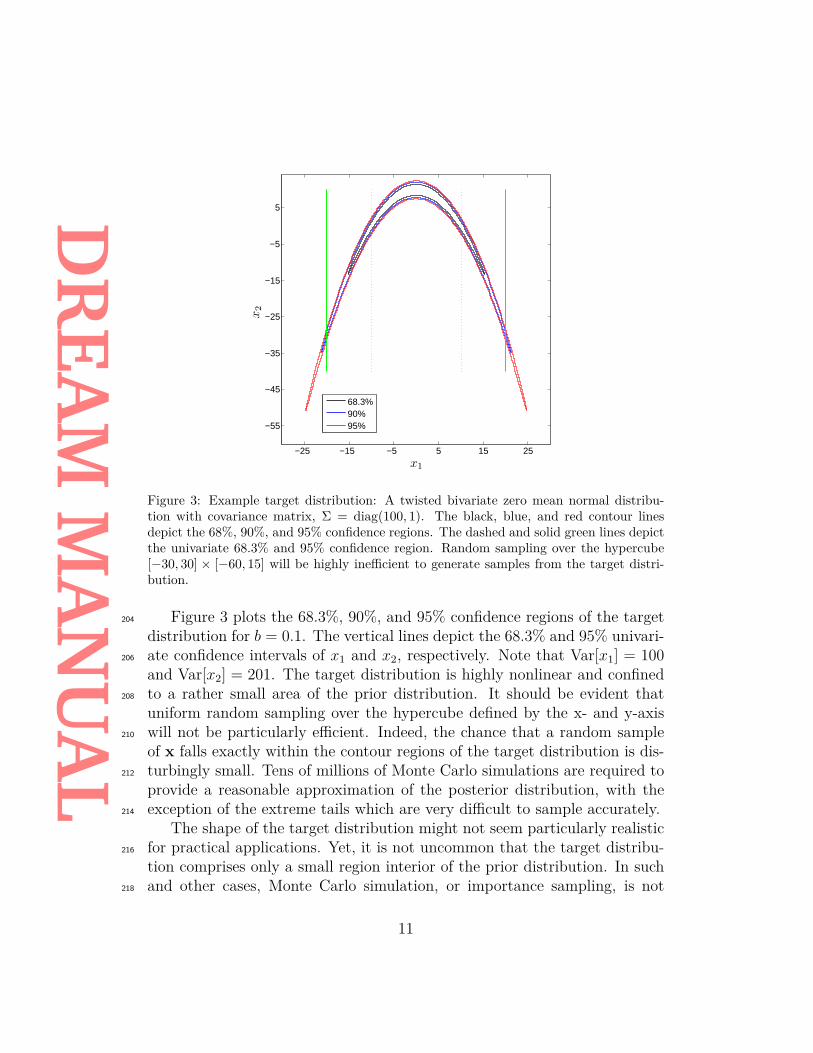
Figure 3: Example target distribution: A twisted bivariate zero mean normal distribu-tion with covariance matrix, Σ = diag(100, 1). The black, blue, and red contour linesdepict the 68%, 90%, and 95% confidence regions. The dashed and solid green lines depictthe univariate 68.3% and 95% confidence region. Random sampling over the hypercube[−30, 30] × [−60, 15] will be highly inefficient to generate samples from the target distri-bution.
Figure 3 plots the 68.3%, 90%, and 95% confidence regions of the target204
distribution for b = 0.1. The vertical lines depict the 68.3% and 95% univari-ate confidence intervals of x1 and x2, respectively. Note that Var[x1] = 100206
and Var[x2] = 201. The target distribution is highly nonlinear and confinedto a rather small area of the prior distribution. It should be evident that208
uniform random sampling over the hypercube defined by the x- and y-axiswill not be particularly efficient. Indeed, the chance that a random sample210
of x falls exactly within the contour regions of the target distribution is dis-turbingly small. Tens of millions of Monte Carlo simulations are required to212
provide a reasonable approximation of the posterior distribution, with theexception of the extreme tails which are very difficult to sample accurately.214
The shape of the target distribution might not seem particularly realisticfor practical applications. Yet, it is not uncommon that the target distribu-216
tion comprises only a small region interior of the prior distribution. In suchand other cases, Monte Carlo simulation, or importance sampling, is not218
11

DR
EAM
MA
NU
AL
particularly appealing. We therefore resort to Markov chain Monte Carlosimulation to explore the posterior target distribution.220
2.2. Markov Chain Monte Carlo simulationThe basis of MCMC simulation is a Markov chain that generates a ran-222
dom walk through the search space and successively visits solutions withstable frequencies stemming from a stationary distribution π. To explore224
the target distribution, a MCMC algorithm generates trial moves from thecurrent state of the Markov chain xt−1 to a new state xp. The earliest and226
most general MCMC approach is the random walk Metropolis (RWM) algo-rithm introduced by Metropolis et al. (1953). This scheme is constructed to228
maintain detailed balance with respect to π(·) at each step in the chain. Ifp(xt−1) (p(xp)) denotes the probability to find the system in state xt−1 (xp)230
and q(xt−1 → xp) (q(xp → xt−1)) is the conditional probability to perform atrial move from xt−1 to xp (xp to xt−1), then the probability pacc(xt−1 → xp)232
to accept the trial move from xt−1 to xp is related to pacc(xp → xt−1) accord-ing to234
p(xt−1)q(xt−1 → xp)pacc(xt−1 → xp) = p(xp)q(xp → xt−1)pacc(xp → xt−1)(7)
If we assume a symmetric jumping distribution, that is q(xt−1 → xp) =236
q(xp → xt−1), then it follows that
pacc(xt−1 → xp)pacc(xp → xt−1) = p(xp)
p(xt−1) (8)238
This Equation does not yet fix the acceptance probability. Metropolis et al.(1953) made the following choice240
pacc(xt−1 → xp) = min[1, p(xp)p(xt−1)
], (9)
to determine whether to accept a trial move or not. This selection rule242
has become the basic building block of many existing MCMC algorithms.Hastings (1970) extended Equation (9) to the more general case of non-244
symmetrical jumping distributions
pacc(xt−1 → xp) = min[1, p(xp)q(xp → xt−1)p(xt−1)q(xt−1 → xp)
], (10)246
12

DR
EAM
MA
NU
AL
in which the forward (xt−1 to xp) and backward (xp to xt−1) jump do nothave equal probability, q(xt−1 → xp) 6= q(xp → xt−1). This generalization is248
known as the Metropolis-Hastings (MH) algorithm and broadens significantlythe type of proposal distribution that can be used for posterior inference.250
The core of the RWM algorithm can be coded in just a few lines (seeFigure 4) and requires only a jumping distribution, a function to generate252
uniform random numbers, and a function to calculate the probability densityof each proposal.254
function [x,p_x] = rwm(prior,pdf,T,d)% Random Walk Metropolis (RWM) algorithm
q = @(C,d) mvnrnd(zeros(1,d),C); % Multivariate normal proposal distributionC = (2.38/sqrt(d))^2 * eye(d); % Covariance matrix proposal distributionx = nan(T,d); p_x = nan(T,1); % Preallocate memory for chain and densityx(1,1:d) = prior(1,d); % Initialize chain by sampling from priorp_x(1) = pdf(x(1,1:d)); % Calculate density current state chain
for t = 2:T, % Dynamic part: Chain evolutionxp = x(t−1,1:d) + q(C,d); % Create candidate pointp_xp = pdf(xp); % Calculate density of proposalalpha = min(p_xp/p_x(t−1),1); % Compute Metropolis ratioidx = alpha > rand; % Alpha larger than U[0,1] or not?if idx, % Idx = 0 (false) or 1 (true)
x(t,1:d) = xp; p_x(t) = p_xp; % True: accept proposalelse
x(t,1:d) = x(t−1,1:d); p_x(t) = p_x(t−1); % False: stay at current state of chainend
end
Figure 4: MATLAB function script of the Random Walk Metropolis (RWM) algorithm.Notation matches variable names used in main text. Based on input arguments prior, pdf,T and d, the RWM algorithm creates a Markov chain, x and corresponding densities, p_x.prior() is an anonymous function that draws N samples from a d-variate prior distribution.This function generates the initial state of the Markov chain. pdf() is another anonymousfunction that computes the density of the target distribution for a given vector of parametervalues, x. Input arguments T and d signify the number of samples of the Markov chainand dimensionality of the parameter space, respectively. Built-in functions are highlightedwith a low dash. The function handle q(C,d) is used to draw samples from a d-variatenormal distribution, mvnrnd() with zero mean and covariance matrix, C. rand draws avalue from a standard uniform distribution on the open interval (0, 1), min() returns thesmallest element of two different scalars, zeros() creates a zeroth vector (matrix), eye()computes the d × d identity matrix, sqrt() calculates the square root, and nan() fillseach entry of a vector (matrix) with not a number.
In words, assume that we have already sampled points {x0, . . . ,xt−1}then the RWM algorithm proceeds as follows. First, a candidate point xp256
is sampled from a proposal distribution q that depends on the present loca-tion, xt−1 and is symmetric, q(xt−1,xp) = q(xp,xt−1). Next, the candidate258
point is either accepted or rejected using the Metropolis acceptance prob-
13

DR
EAM
MA
NU
AL
ability (Equation 9). Finally, if the proposal is accepted the chain moves260
to xp, otherwise the chain remains at its current location xt−1. Repeatedapplication of these three steps results in a Markov chain which, under cer-262
tain regularity conditions, has a unique stationary distribution with posteriorprobability density function, π(·). In practice, this means that if one looks264
at the values of x sufficiently far from the arbitrary initial value, that is,after a burn-in period, the successively generated states of the chain will be266
distributed according to the underlying posterior probability distribution ofx, π(·). Burn-in is required to allow the chain to explore the search space268
and reach its stationary regime.Figure 5 illustrates the outcome of the RWM algorithm for a simple d = 2-270
dimensional multivariate normal target distribution with correlated dimen-sions. This target distribution is specified as anonymous function (a function272
not stored as program file) in MATLAB
pdf = @(x) mvnpdf(x,[0 0],[1 0.8; 0.8 1]) (11)274
where the @ operator creates the handle, and the parentheses contain theactual function itself. This anonymous function accepts a single input x, and276
implicitly returns a single output, a vector (or scalar) of posterior densityvalues with same number of rows as x.278
The chain is initialized by sampling from U2[−10, 10], where Ud(a, b) de-notes the d-variate uniform distribution with lower and upper bounds a and280
b, respectively, and thus
prior = @(N,d) unifrnd(-10,10,N,d) (12)282
The left graph presents a scatter plot of the bivariate posterior samples usinga total of T = 50, 000 function evaluations and burn-in of 50%. The contours284
depict the 68, 90, and 95% uncertainty intervals of the target distribution.The right graph displays a trace plot of the sampled chain trajectory.286
14

DR
EAM
MA
NU
AL
−4 −2 0 2 4−4
−3
−2
−1
0
1
2
3
4
x1
x2
(A)
(A)
−3
−1
1
3
x1
(B)
0 10,000 20,000 30,000 40,000 50,000
−3
−1
1
3
x2
Sample of Markov chain
(C)
Figure 5: (A) bivariate scatter plots of the RWM derived posterior samples. The green,black and blue contour lines depict the true 68, 90 and 95% uncertainty intervals of thetarget distribution, respectively. (B,C) trace plots of the sampled values of x1 (top) andx2 (bottom).
Perhaps not surprisingly, the bivariate samples of the RWM algorithmnicely approximate the target distribution. The acceptance rate of XX% is288
somewhat low but certainly higher than derived from Monte Carlo simula-tion. The posterior mean and covariance are in excellent agreement with290
those used for the target distribution (not shown).This simple example just serves to demonstrate the ability of RWM to292
approximate the posterior target distribution. The relative ease of imple-mentation of RWM and its theoretical underpinning have led to widespread294
application and use in Bayesian inference. However, the efficiency of theRWM algorithm is determined by the choice of the proposal distribution,296
q(·) used to create trial moves (transitions) in the Markov chain. When theproposal distribution is too wide, too many candidate points are rejected,298
and therefore the chain will not mix efficiently and converge only slowly tothe target distribution. On the other hand, when the proposal distribution is300
too narrow, nearly all candidate points are accepted, but the distance movedis so small that it will take a prohibitively large number of updates before the302
sampler has converged to the target distribution. The choice of the proposaldistribution is therefore crucial and determines the practical applicability of304
MCMC simulation in many fields of study (Owen and Tribble, 2005).
15

DR
EAM
MA
NU
AL
3. Automatic tuning of proposal distribution306
In the past decade, a variety of different approaches have been proposed toincrease the efficiency of MCMC simulation and enhance the original RWM308
and MH algorithms. These approaches can be grouped into single and mul-tiple chain methods.310
3.1. Single-chain methodsThe most common adaptive single chain methods are the adaptive pro-312
posal Haario et al. (1999), adaptive Metropolis (AM) Haario et al. (2001)and delayed rejection adaptive metropolis (DRAM) algorithm (Haario et314
al., 2006), respectively. These methods work with a single trajectory, andcontinuously adapt the covariance, Σ of a Gaussian proposal distribution,316
qt(xt−1, ·) = Nd(xt−1, sdΣ) using the accepted samples of the chain, Σ =cov(x0, . . . ,xt−1) + εId. The variable sd represents a scaling factor (scalar)318
that depends only on the dimensionality d of the problem, Id signifies the d-dimensional identity matrix, and ε = 10−6 is a small scalar that prevents the320
sample covariance matrix to become singular. As a basic choice, the scalingfactor is chosen to be sd = 2.382/d which is optimal for Gaussian target and322
proposal distributions (Gelman et al., 1996; Roberts et al., 1997) and shouldgive an acceptance rate close to 0.44 for d = 1, 0.28 for d = 5 and 0.23 for324
large d.
16

DR
EAM
MA
NU
AL
function [x,p_x] = am(prior,pdf,T,d)% Adaptive Metropolis (AM) algorithm
q = @(C,d) mvnrnd(zeros(1,d),C); % Proposal distributionC = (2.38/sqrt(d))^2 * eye(d); % Covariance matrix proposal distributionx = nan(T,d); p_x = nan(T,1); % Preallocate memory for chain and densityx(1,1:d) = prior(1,d); % Initialize chain by sampling from priorp_x(1) = pdf(x(1,1:d)); % Calculate density current state chain
for t = 2:T, % Dynamic part: Chain evolution% −−−−−−− Adaptation covariance matrix of proposal distribution −−−−−−−if mod(t,100)
C = (2.38/sqrt(d))^2 * (cov(x(1:t−1,1:d)) + 1e−6*eye(d));% Note: recursive formulae for C much more CPU−efficient!
end% −−−−−−−−−−−−−−−−−−−−−−−− End adaptation −−−−−−−−−−−−−−−−−−−−−−−−−−−−−xp = x(t−1,1:d) + q(C,d); % Create candidate pointp_xp = pdf(xp); % Calculate density of proposalalpha = min(p_xp/p_x(t−1),1); % Compute Metropolis ratioidx = alpha > rand; % Alpha larger than U[0,1] or not?if idx, % Idx = 0 (false) or 1 (true)
x(t,1:d) = xp; p_x(t) = p_xp; % True: accept proposalelse
x(t,1:d) = x(t−1,1:d); p_x(t) = p_x(t−1); % False: stay at current state of chainend
end
Figure 6: Basic MATLAB code of adaptive Metropolis (AM) algorithm. This code issimilar to that of the RWM algorithm in Figure 1 but the d × d covariance matrix, C ofthe proposal distribution, q() is adapted using the samples stored in the Markov chain.Built-in functions are highlighted with a low dash. mod() signifies the modulo operation,and cov() computes the covariance matrix of the chain samples, x.
Single-site updating of x (Haario et al., 2005) is possible to increase ef-326
ficiency of AM for high-dimensional problems (large d). In addition, for thespecial case of hierarchical Bayesian inference of hydrologic models, Kucz-328
era et al. (2010) proposed to tune Σ using a limited-memory multi-blockpre-sampling step, prior to a classical single block Metropolis run.330
The use of a multivariate normal proposal distribution with covariancematrix adaptation works well for Gaussian-shaped target distributions, but332
cannot sample adequately multimodal distributions with long tails, possiblyinfinite first and second moments. A simple two-dimensional toy example,334
presented later will demonstrate the convergence problems of AM on multi-modal target distributions. Moreover, a single chain is unable to efficiently336
cope with these peculiarities, and traverse rapidly through multi-dimensionalparameter spaces with multiple different regions of attraction and numerous338
local optima in pursuit of the target distribution. Monitoring convergence ofa single chain is also difficult. For example, it is relatively easy for a single-340
chain to become stuck in a local mode and common diagnostics would notdetect that the chain has not explored adequately the full posterior mod-342
17

DR
EAM
MA
NU
AL
el/parameter space Gelman and Shirley (2009). As alternative to AM onecan assume a fixed covariance matrix (identity matrix) but with jump rate344
tuned adaptively during burn-in so that a desired theoretical acceptance rateis achieved. This approach is easy to implement but suffers from the same346
problems as the AM algorithm.
3.2. Multi-chain methods: DE-MC348
Multiple chain methods use different trajectories running in parallel toexplore the posterior target distribution. The use of multiple chains has350
several desirable advantages, particularly when dealing with complex poste-rior distributions involving long tails, correlated parameters, multi-modality,352
and numerous local optima (Gilks et al., 1994; Liu et al., 2000; ter Braak,2006; ter Braak and Vrugt, 2008; Vrugt et al., 2009; Radu et al., 2009). The354
use of multiple chains offers a robust protection against premature conver-gence, and opens up the use of a wide arsenal of statistical measures to356
test whether convergence to a limiting distribution has been achieved (Gel-man and Rubin, 1992). One popular multi-chain method that has found358
widespread application and use in hydrology is the Shuffled Complex Evo-lution Metropolis algorithm (SCEM-UA, Vrugt et al., 2003). Although the360
proposal adaptation of SCEM-UA violates Markovian properties, numericalbenchmark experiments on a diverse set of multi-variate target distributions362
have shown that the method is efficient and close to exact. The differencebetween the limiting distribution of SCEM-UA and the true target distribu-364
tion is negligible in most reasonable cases and applications. The SCEM-UAmethod can be made exact if the multi-chain adaptation of the covariance366
matrix is applied only during burn-in. Similar to AP (Haario et al., 1999),the method is then used to derive an efficient Gaussian proposal distribution368
for the standard Metropolis algorithm. Nevertheless, we do not consider thisalgorithm herein.370
ter Braak (2006) proposed a simple adaptive RWM algorithm called Dif-ferential Evolution Markov chain (DE-MC). DE-MC uses differential evolu-372
tion as genetic algorithm for population evolution with a Metropolis selectionrule to decide whether candidate points should replace their parents or not.374
In DE-MC, N different Markov chains are run simultaneously in parallel. Ifthe state of a single chain is given by the d-vector x, then at each generation376
t− 1 the N chains in DREAM define a population X, which corresponds toan N×d matrix, with each chain as a row. Multivariate proposals are gener-378
ated on the fly from the collection of chains, Xt−1 using differential evolution
18
DR
EAM
MA
NU
AL
(Storn and Price, 1997; Price et al., 2005)380
xip = γd(xr1t−1 − xr2
t−1) + ed, r1 6= r2 6= i, (13)
where γ is the jump rate, r1 and r2 are integer values drawn without re-382
placement from {1, . . . , i− 1, i+ 1, . . . , N}, and e ∼ Nd(0, b) is drawn from anormal distribution with small b, say b = 10−6. By accepting each proposal384
with Metropolis probability, α(xit−1,xip) = min(p(xip)/p(xit−1), 1) a Markovchain is obtained the stationary or limiting distribution of which is the pos-386
terior distribution. The proof of this is given in ter Braak and Vrugt (2008).Because the joint pdf of the N chains factorizes to π(x1|·)× . . .×π(xN |·), the388
states x1 . . .xN of the individual chains are independent at any generationafter DE-MC has become independent of its initial value. After this burn-in390
period, the convergence of a DE-MC run can thus be monitored with theR-statistic of Gelman and Rubin (1992). If the initial population is drawn392
from the prior distribution, then DE-MC translates this sample into a pos-terior population. From the guidelines of sd in RWM the optimal choice of394
γ = 2.38/√
2d. With a probability of 10% we use γ = 1, or p(γ=1) = 0.1 toallow for mode-jumping (ter Braak, 2006; ter Braak and Vrugt, 2008; Vrugt396
et al., 2008a, 2009) which is a significant strength of DE-MC as will be shownlater. If the posterior distribution consists of disconnected modes with in-398
between regions of low probability, covariance based MCMC methods will beslow to converge as transitions between probability regions will be infrequent.400
The DE-MC method can be coded in MATLAB in about 20 lines (Fig-ure 7), and solves an important practical problem in RWM, namely that of402
choosing an appropriate scale and orientation for the jumping distribution.Earlier approaches such as (parallel) adaptive direction sampling (Gilks et404
al., 1994; Roberts and Gilks, 1994; Gilks and Roberts, 1996) solved the orien-tation problem but not the scale problem.406
19
DR
EAM
MA
NU
AL
function [x,p_x] = de_mc(prior,pdf,N,T,d)% Differential Evolution Markov Chain (DE−MC) algorithm
gamma_RWM = 2.38/sqrt(2*d); % Calculate jump rate (RWM based)x = nan(T,d,N); p_x = nan(T,N); % Preallocate memory for chains and densityX = prior(N,d); p_X = pdf(X); % Create initial population and compute densityx(1,1:d,1:N) = reshape(X',1,d,N); p_x(1,1:N) = p_X'; % Store initial position of chain and densityfor i = 1:N, R(i,1:N−1) = setdiff(1:N,i); end % R−matrix: ith chain, the index of chains for DE
for t = 2:T, % Dynamic part: Evolution of N chains[~,draw] = sort(rand(N−1,N)); % Randomly permute [1,...,N−1] N timesg = randsample([gamma_RWM 1],1,true,[0.9 0.1]); % Set gamma: 2.38/sqrt(2d) or 1, 90/10 ratiofor i = 1:N, % Create proposal and accept/reject
r1 = R(i,draw(1,i)); % Derive r1r2 = R(i,draw(2,i)); % Derive r2; r1 not equal r2 not equal iXp(i,1:d) = X(i,1:d) + g*(X(r1,1:d)−X(r2,1:d))...
+ 1e−6*randn(1,d); % Create ith point with differential evolutionp_Xp(i,1) = pdf(Xp(i,1:d)); % Calculate density of ith proposalalpha = min(p_Xp(i,1)/p_X(i,1),1); % Compute Metropolis ratioidx = alpha > rand; % Alpha larger than U[0,1] or not?if idx,
X(i,1:d) = Xp(i,1:d); p_X(i,1) = p_Xp(i,1); % True: Accept proposalend
endx(t,1:d,1:N) = reshape(X',1,d,N); p_x(t,1:N) = p_X'; % Add current position and density to chain
end
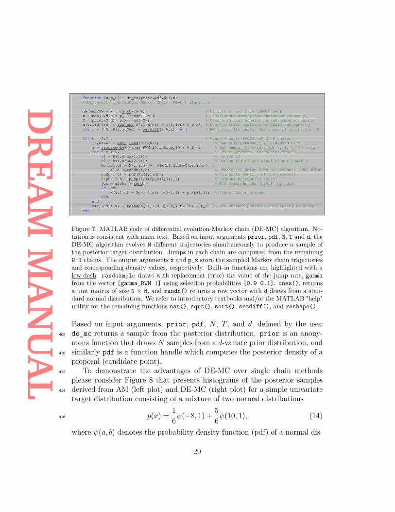
Figure 7: MATLAB code of differential evolution-Markov chain (DE-MC) algorithm. No-tation is consistent with main text. Based on input arguments prior, pdf, N, T and d, theDE-MC algorithm evolves N different trajectories simultaneously to produce a sample ofthe posterior target distribution. Jumps in each chain are computed from the remainingN-1 chains. The output arguments x and p_x store the sampled Markov chain trajectoriesand corresponding density values, respectively. Built-in functions are highlighted with alow dash. randsample draws with replacement (true) the value of the jump rate, gammafrom the vector [gamma_RWM 1] using selection probabilities [0.9 0.1]. ones(), returnsa unit matrix of size N × N, and randn() returns a row vector with d draws from a stan-dard normal distribution. We refer to introductory textbooks and/or the MATLAB "help"utility for the remaining functions nan(), sqrt(), sort(), setdiff(), and reshape().
Based on input arguments, prior, pdf, N , T , and d, defined by the userde_mc returns a sample from the posterior distribution. prior is an anony-408
mous function that draws N samples from a d-variate prior distribution, andsimilarly pdf is a function handle which computes the posterior density of a410
proposal (candidate point).To demonstrate the advantages of DE-MC over single chain methods412
please consider Figure 8 that presents histograms of the posterior samplesderived from AM (left plot) and DE-MC (right plot) for a simple univariate414
target distribution consisting of a mixture of two normal distributions
p(x) = 16ψ(−8, 1) + 5
6ψ(10, 1), (14)416
where ψ(a, b) denotes the probability density function (pdf) of a normal dis-
20

DR
EAM
MA
NU
AL
tribution with mean a and standard deviation b. The target distribution is418
displayed with a sold black line, and equivalent topdf = @(x) 1/6*normpdf(x,-8,1) + 5/6*normpdf(x,10,1) (15)420
The initial state of the Markov chain(s) is sampled from U [−20, 20] usingprior = @(N,d) unifrnd(-20,20,N,d).422
The AM algorithm produces a spurious approximation of the bimodaltarget distribution. The variance (width) of the proposal distribution is424
insufficient to enable the chain to adequately explore both modes of the targetdistribution. A simple remedy to this problem is to increase the (default)426
initial variance of the univariate normal proposal distribution. This wouldallow the AM sampler to take much larger steps and jump directly between428
both modes, but at the expense of a drastic reduction in the acceptance rateand search efficiency. Indeed, besides the occasional successful jumps many430
other proposals will overshoot the target distribution, and be rejected.This rather simple univariate example illustrates the dilemma of RWM432
how to determine an appropriate scale and orientation of the proposal distri-bution. Fortunately, the histogram of the posterior samples derived with the434
DE-MC algorithm matches perfectly the mixture distribution. Periodic useof γ = 1 enables the N = 10 different Markov chains of DE-MC to transition436
directly between the two disconnected posterior modes (e.g. ter Braak andVrugt (2008); Vrugt et al. (2008a); Laloy and Vrugt (2012a)) and rapidly438
converge to the exact target distribution.
−10 0 100
0.1
0.2
0.3
0.4
Den
sity
(A) AM
x−10 0 10
(B) DE−MC
x
Figure 8: Histogram of the posterior distribution derived from the (A) AM (single chain),and (B) DE-MC (multi-chain) samplers. The solid black line displays the pdf of the truemixture target distribution.
21

DR
EAM
MA
NU
AL
In previous work (Vrugt et al., 2008a, 2009) we have shown that the effi-440
ciency of DE-MC can be enhanced, sometimes dramatically, by using adap-tive randomized subspace sampling, multiple chain pairs for proposal cre-442
ation, and explicit consideration of aberrant trajectories. This method, enti-tled DiffeRential Evolution Adaptive Metropolis (DREAM) maintains de-444
tailed balance and ergodicity and has shown to exhibit excellent performanceon a wide range of problems involving nonlinearity, high-dimensionality, and446
multimodality. In these and other papers [e.g (Laloy and Vrugt, 2012a)]benchmark experiments have shown that DREAM outperforms other adap-448
tive MCMC sampling approaches, and, in high-dimensional search/variablespaces, can even provide better solutions than commonly used optimization450
algorithms.
3.3. Multi-chain methods: DREAM452
The DREAM algorithm has it roots within DE-MC but uses subspacesampling and outlier chain correction to speed up convergence to the target454
distribution. Subspace sampling is implemented in DREAM by only updat-ing randomly selected dimensions of xit−1 each time a proposal is generated.456
If A is a subset of D-dimensions of the original parameter space, RD ⊆ Rd,then a jump in the ith chain, i = {1, . . . , N} at iteration t = {2, . . . , T}458
is calculated using different evolution (Storn and Price, 1997; Price et al.,2005)460
dxi,A =(1D + λD)γ(δ,D)
δ∑j=1
(xr1
j ,A
t−1 − xr2j ,A
t−1
)+ ζD
dxi, 6=A =0,(16)
where γ = 2.38/√
2δD is the jump rate, δ denotes the number of chain pairs462
used to generate the jump (default is 3), and r1 and r2 are vectors consistingof δ integer values drawn without replacement from {1, . . . , i−1, i+1, . . . , N}.464
The values of λ and ζ are sampled independently from UD(−c, c) andND(0, c∗) with, typically, c = 0.1 and c∗ small compared to the width of466
the target distribution, c∗ = 10−12 say. With a probability of 20% we setthe jump rate to 1, or p(γ=1) = 0.2 to enable jumping between disconnected468
posterior modes. The candidate point of chain i at iteration t then becomes
xip = xit−1 + dxi, (17)470
and the Metropolis ratio is used to determine whether to accept this proposalor not.472
22

DR
EAM
MA
NU
AL
In DREAM a geometric series of ncr different crossover values is used,CR = { 1
ncr, 2ncr, . . . , 1}. The selection probability of each crossover value474
is assumed equal at the start of simulation and defines a vector pcr withncr copies of 1
ncr. For each different proposal the crossover, cr is sampled476
randomly from a discrete multinomial distribution, cr = F(CR, 1,pcr). Then,a vector z = {z1, . . . , zd} with d standard uniform random labels is drawn478
from a standard multivariate uniform distribution, z ∼ Ud(0, 1). All thosedimensions j for which zj ≤ cr are stored in A and span the subspace that480
will be sampled. In the case that A is empty, one dimension of xt−1 will besampled at random.482
The number of dimensions stored in A ranges between 1 and d and de-pends on the actual crossover value used. This randomized strategy, activated484
when cr < 1, constantly introduces new directions that chains can take out-side the subspace spanned by their current positions. This relatively simple486
randomized selection strategy enables single-site Metropolis sampling (onedimension at a time), Metropolis-within-Gibbs (one or a group of dimen-488
sions) and regular Metropolis sampling (all dimensions). In principle, thisallows using N < d in DREAM, an important advantage over DE-MC that490
requires N = 2d chains to be run in parallel (ter Braak, 2006).The core of the DREAM algorithm can be written in MATLAB in about492
30 lines of code (see Figure 9). The input arguments are similar to thoseof the de-mc code and include the function handles prior and pdf and the494
values of N , T , and d.
23

DR
EAM
MA
NU
AL
function [x,p_x] = dream(prior,pdf,N,T,d)% DiffeRential Evolution Adaptive Metropolis (DREAM) algorithm
[delta,c,c_star,nCR,p_g] = deal(3,0.1,1e−12,3,0.2); % Default values DREAM algorithmic parametersx = nan(T,d,N); p_x = nan(T,N); % Preallocate memory for chains and densityX = prior(N,d); p_X = pdf(X); % Create initial population and compute densityx(1,1:d,1:N) = reshape(X',1,d,N); p_x(1,1:N) = p_X'; % Store initial position of chain and densityfor i = 1:N, R(i,1:N−1) = setdiff(1:N,i); end % R−matrix: ith chain, the index of chains for DECR = [1:nCR]/nCR; pCR = ones(1,nCR)/nCR; % Crossover values and their selection probability
for t = 2:T, % Dynamic part: Evolution of N chains[~,draw] = sort(rand(N−1,N)); % Randomly permute [1,...,N−1] N timesdx = zeros(N,d); % Set N jump vectors equal to zerolambda = unifrnd(−c,c,N,1); % Draw N lambda valuesfor i = 1:N, % Create proposal each chain and accept/reject
r1 = R(i,draw(1:delta,i)); % Derive vector r1r2 = R(i,draw(delta+1:2*delta,i)); % Derive vector r2cr = randsample(CR,1,true,pCR); % Select crossover valueA = find(rand(1,d) < cr); % Derive subset A with dimensions to sampleD = numel(A); % How many dimensions are sampled?gamma_D = 2.38/sqrt(2*delta*D); % Calculate jump rateg = randsample([gamma_D 1],1,true,[1−p_g p_g]); % Select gamma: 80/20 ratio (default)dx(i,A) = (1+lambda(i))*g*sum(X(r1,A)−...
X(r2,A),1) + c_star*randn(1,D); % Compute ith jump with differential evolutionXp(i,1:d) = X(i,1:d) + dx(i,1:d); % Compute ith proposalp_Xp(i,1) = pdf(Xp(i,1:d)); % Calculate density of ith proposalalpha = min(p_Xp(i,1)./p_X(i,1),1); % Compute Metropolis ratioidx = alpha > rand; % Alpha larger than U[0,1] or not?if idx,
X(i,1:d) = Xp(i,1:d); p_X(i,1) = p_Xp(i,1); % True: Accept proposalend
end[X,p_X] = outlier(X,log(p_x(ceil(t/2):t,1:N))); % Outlier detection and correctionx(t,1:d,1:N) = reshape(X',1,d,N); p_x(t,1:N) = p_X'; % Add current position and density to chain
end
Figure 9: MATLAB code of the differential evolution adaptive Metropolis (DREAM) al-gorithm. The script is similar to that of DE-MC but uses (a) more than one chain pairto create proposals, (b) subspace sampling, and (c) outlier chain detection, to enhanceconvergence to the posterior target distribution. Built-in functions are highlighted witha low dash. The jump vector, dx(i,1:d) of the ith chain contains the desired infor-mation about the scale and orientation of the proposal distribution and is derived fromthe remaining N-1 chains. deal() assigns default values to the algorithmic variables ofDREAM. sum() computes the sum of the columns A of the chain pairs r1 and r2. Thefunction outlier() computes the mean of the log posterior density of the samples in thesecond half of each of the Markov chains. These N values make up a distribution andcan be checked for outliers using common statistical tests such as the interquartile range(among others). The states of aberrant trajectories are subsequently reset and samplesdiscarded through burn-in.
The performance of DE-MC and DREAM can suffer from one critical496
deficiency. If one of the N chains is trapped in a local minimum sufficientlyfar removed from the target distribution then the search can stagnate because498
the outlier chain is unable to reach the posterior and join the other N −1 chains (ter Braak and Vrugt, 2008; Vrugt et al., 2009). This happens500
if the differences between the states of the chains that sample the target
24

DR
EAM
MA
NU
AL
distribution are too small to enable the aberrant chain to jump outside the502
space spanned by the local optimum and move in the direction of the posteriordistribution. This deteriorates search efficiency and prohibits convergence to504
a limiting distribution. The function outlier corrects the state of aberranttrajectories by comparing the mean log-density values of the last 50% of the506
samples of the N different Markov chains. Details can be found in (Vrugt etal., 2009).508
To enhance search efficiency, the probability, pcr of each of the ncr crossovervalues is tuned adaptively during burn-in by maximizing the normalized510
Euclidean distance between successively sampled states of the N differentchains. Details of this approach can be found in Vrugt et al. (2008a, 2009).512
The default value of ncr = 3, works well for most sampling problems, yetlarger values are recommended for high-dimensional parameter spaces, d >514
50.The MATLAB code of DREAM in Figure 9 uses serial updating of the516
N different chains. This numerical implementation is required to satisfyDREAM’s (DE-MC) reversibility proof (ter Braak and Vrugt, 2008; Vrugt et518
al., 2009), but impairs parallelization and thus effective use of multi-processorresources. Fortunately, benchmark experiments demonstrate excellent results520
(posterior estimates) if all of the N proposals are created jointly prior to ap-plication of the Metropolis selection rule. This alternative approach enables522
the N candidate points to be evaluated in parallel, thereby permitting in-ference of CPU-intensive forward models. The DREAM software package524
implements an option for multi-core evaluation of the different chains usingthe MATLAB parallel computing toolbox.526
This basic implementation of DREAM is relatively simple, but not par-ticularly user-friendly. Proficient knowledge of statistics, numerical analysis,528
and computer coding is required to be able to modify this rather parsimoniouscode so that it can handle posterior sampling problems involving dynamic530
models, different error residual distributions (likelihood functions), summarystatistics (diagnostic model evaluation), high-dimensional parameter spaces532
(insufficient memory), and CPU-intensive simulators (parallel computing).To simplify application of Bayesian inference and MCMC simulation, I have534
developed a general-purpose MATLAB package of DREAM which includesmany different functionalities and post-processing capabilities. These options536
can be activated in an input file, and avoids users to have to make changesto the core of the algorithm itself. The next sections of this paper will dis-538
cuss the DREAM package, and uses several examples to illustrate how the
25

DR
EAM
MA
NU
AL
package can be used to solve a wide variety of inference problems.540
4. MATLAB implementation of DREAM
The basic code of DREAM listed in Figure 9 was written in 2006 but542
many new functionalities and options have been added to the source codein recent years due to continued research developments and to support the544
needs of a growing group of users. The DREAM code can be executed fromthe MATLAB prompt by the command546
[chain,output,fx] = DREAM(Func_name,DREAMPar,Par_info)
where Func_name (string), DREAMPar (structure array), and Par_info (struc-548
ture array) are input arguments defined by the user, and chain (matrix),output (structure array) and fx (matrix) are output variables computed by550
DREAM and returned to the user. To minimize the number of input andoutput arguments in the DREAM function call and related primary and sec-552
ondary functions called by this program, we use MATLAB structure arraysand group related variables in one main element using data containers called554
fields, more of which later. Two optional input arguments that the user canpass to DREAM are Meas_info and options and their content and usage556
will be discussed below.The DREAM function uses more than twenty other functions to help558
generate samples from the posterior distribution. All these functions aresummarized briefly in Appendix A. In the subsequent sections I will dis-560
cuss the MATLAB implementation of DREAM. This, along with prototypecase studies presented herein and template examples listed in runDREAM562
should help users apply Bayesian inference to their data and models.
4.1. Input argument 1: Func_Name564
The variable Func_Name defines the name (enclosed in quotes) of theMATLAB function (.m file) used to calculate the likelihood (or proxy thereof)566
of each proposal. The use of a m-file rather than anonymous function (e.g.pdf), permits DREAM to solve inference problems involving, for example,568
dynamic simulation models. If we conveniently assume Func_name to beequivalent to ’model’ then the call to this function becomes570
Y = model(x) (18)
26

DR
EAM
MA
NU
AL
where x (input argument) is a 1 × d vector of parameter values, and Y is a572
return argument whose content is either a likelihood, log-likelihood, or vectorof simulated values or summary statistics, respectively. The content of the574
function model needs to be written by the user - the syntax definition isuniversal. Appendix C provides six different templates of the function model576
which are used in the case study presented in section 5.
4.2. Input argument 2: DREAMPar578
The structure DREAMPar defines the computational settings of DREAM.Table 1 lists the different fields of DREAMPar, their default values, and the cor-580
responding variable names used in the mathematical description of DREAMin section 3.3.582
Table 1: Main algorithmic variables of DREAM: Mathematical symbols, correspondingfields of DREAMPar and default settings.Symbol Description Field DREAMPar Default
Problem dependentd number of parameters dN number of Markov chains N ≤ 2δ + 1T number of generations TL(x|Y) likelihood function lik [1, 2], [11− 15], [21, 22]
Default settingsncr number of crossover values nCR 3 †δ number of chain pairs proposal delta 3λ randomization lambda 0.1ζ ergodicity zeta 10−12 ‡
p(γ=1) probability unit jump rate p_unit_gamma 0.2outlier detection test outlier ’iqr’
K thinning rate thinning 1adapt crossover probabilities? adapt_pCR ’yes’
m shaping factor (for GLUE) GLUE > 0 §
† λ ∼ Ud(−DREAMPar.lambda, DREAMPar.lambda)‡ ζ ∼ Nd(0, DREAMPar.zeta)§ For Generalized Likelihood Uncertainty Estimation (Beven and Binley, 1992)
The names of the different fields of DREAMPar are equivalent to the sym-bols (letters) used in the (mathematical) description of DREAM (e.g. see584
Equations (16) and (17) ). The values of the fields d, N, T depend on thedimensionality of the target distribution, and hence should be defined by the586
27

DR
EAM
MA
NU
AL
user. Default settings are assumed for the remaining fields of DREAMPar inTable 1 with the exception of variables GLUE and lik that will be discussed in588
the next two paragraphs. To make sure that a sufficient number of chains isavailable to create proposals with the discrete jumping distribution of Equa-590
tion (16), the value of N should at least be set to 2δ+1. For a default value ofδ = 3, then this would require at least N = 7 chains for all considered target592
dimensionalities. This might seem somewhat excessive for low dimensionalproblems, and hence one could conveniently assume δ = 1 for d = 1. Note,594
the default settings of DREAMPar are easily modified by the user, by simplyspecifying individual fields and their respective values.596
The field GLUE of DREAMPar allows the user to specify the value of asubjective shaping factor which is used in the GLUE framework to calcu-598
late the likelihood of each proposal. We will revisit the use of GLUE andinformal Bayesian inference in the next sections. The content of the field lik600
of DREAMPar defines the choice of likelihood function used to compare theoutput of the function model with (observational) data. Table 2 summarizes602
the different options for lik the user can select from. The choice of likelihoodfunction depends in large part on the content of the return argument Y of604
the function model, which could be a (log)-likelihood, vector with simulatedvalues, or vector of summary statistics, respectively.606
28

DR
EAM
MA
NU
AL
Table 2: Built-in likelihood functions of the DREAM package. The value of field lik ofDREAMPar depends on the content of the return argument Y from the function model: [1]likelihood, [2] log-likelihood, [11-16] for one or more simulated values, [21-22] for one ormore summary statistics, and [31-34] informal likelihood functions for simulated values orsummary metrics. The mathematical formulation of each likelihood function is given inAppendix B.
lik Description References1 Likelihood, L(x|Y) e.g. Equation (11)2 Log-likelihood, L(x|Y)11 Gaussian likelihood: measurement error integrated out Thiemann et al. (2001)12 † Gaussian likelihood: homos/heteroscedastic data error Equation (6)13 ‡ Gaussian likelihood: with AR-1 model of error residuals Vrugt et al. (2009)14 § Generalized likelihood function Schoups and Vrugt (2010a)15 Whittle’s likelihood (spectral analysis) Whittle (1953)16 Laplacian likelihood: homos/heteroscedastic data error Laplace (1774)21 ¶ Noisy ABC: Gaussian likelihood Turner and Sederberg (2012)22 ¶ ABC: Boxcar likelihood Sadegh and Vrugt (2014)31 £ Inverse error variance with shaping factor Beven and Binley (1992)32 £ Nash and Sutcliffe efficiency with shaping factor Freer et al. (1996)33 £ Exponential transform error variance with shaping factor Freer et al. (1996)34 £ Sum of absolute error residuals Beven and Binley (1992)
† Measurement data error defined a-priori by user in field sigma of Par_info or inferredjointly with parameters‡ Includes estimation of lag-1 autocorrelation of the error residuals§ Latent variables for model bias, correlation, non-stationarity and nonnormality of errorresiduals¶ Default value of ε = 0.025 is used to separate behavioral and non-behavioral samples£ Informal likelihood with shaping factor defined in field GLUE of DREAMPar.
If the content of the return argument, Y of function model is a likelihoodor log-likelihood then field lik of DREAMPar is equivalent to 1 or 2, respec-608
tively. This choice is often appropriate for benchmark problems involving(among others) some known multivariate probability density function, ex-610
amples of which are Equation (14), and case studies 1 and 2 presented insection 5. Likelihood functions 11-16 (and 31-34) are appropriate if the out-612
put of model consists of a vector (or scalar) of simulated values of sometemporally/spatially varying property. These likelihood functions differ in614
their underlying assumptions regarding the probabilistic properties of theerror residuals, and some (12-14,16) contain latent variables whose values616
can be estimated along with x, the parameters of a system model. Finally,
29

DR
EAM
MA
NU
AL
likelihood functions 21 and 22 assume the content of the return argument Y618
of model to consist of one or more (simulated) summary statistics. Section5 presents the application of different likelihood functions and provides tem-620
plates for their use. Appendix B provides the mathematical formulation ofeach of the likelihood functions listed in Table 2.622
The generalized likelihood (GL) function of Schoups and Vrugt (2010a)(14) is most versatile in that it accounts explicitly for bias, correlation, non-624
stationarity, and nonnormality of the error residuals using latent variables.Whittle’s likelihood (Whittle, 1953) (15) is a frequency-based approximation626
of the Gaussian likelihood and can be interpreted as minimum distance esti-mate of the distance between the parametric spectral density and the (non-628
parametric) periodogram. It also minimises the asymptotic Kullback-Leiblerdivergence and, for autoregressive processes, provides asymptotically consis-630
tent estimates for Gaussian and non-Gaussian data, even in the presenceof long-range dependence (Montanari and Toth, 2007). Likelihood function632
16, also referred to as the Laplace or double exponential distribution, differsfrom all other likelihood functions (except 14) in that it assumes a L1-norm634
of the error residuals. In practice this means that all residuals are weightedequally and that the inference is not as sensitive to outliers. Likelihood func-636
tions 31-34 are implemented for proponents of the GLUE methodology ofBeven and Binley (1992). The mathematical formulation of these informal638
likelihood functions appears in Beven and Binley (1992), Freer et al. (1996),and Beven and Freer (2001) (among others). The use of DREAM with infor-640
mal likelihood functions significantly enhances, sometimes dramatically, thecomputational efficiency of GLUE (Blasone et al., 2008). The script run-642
DREAM provides several example applications of the different likelihoodfunctions.644
The field thinning of DREAMPar allows the user to specify the thinning rateof each Markov chain to reduce memory requirements for high-dimensional646
target distributions. For instance, for a d = 100 dimensional target distri-bution with N = 100 and T = 10, 000, MATLAB would need a staggering648
100-million bytes of memory to store all the samples of the joint chains.Thinning applies to all the sampled chains, and stores only every Kth vis-650
ited state. This option reduces memory storage with a factor of T/K, andalso decreases the autocorrelation between successively stored chain samples.652
A default value of K = 1 (no thinning) is assumed in DREAM. Note, largevalues for K (K » 10) can be rather wasteful because many visited states654
are not used in the computation of the posterior moments and/or plotting
30

DR
EAM
MA
NU
AL
of marginal/bivariate parameter distributions.656
Chains that sample local areas of the posterior distribution can frustrateconvergence of DREAM (or any other sampling algorithm) tof a limiting dis-658
tribution. Such outlier chains are often the consequence of poor model nu-merics, for instance, explicit solvers with a too large integration time step are660
known to produce spurious local optima (Clark and Kavetski, 2010; Schoupset al., 2010b). The field outlier of DREAMPar contains (in quotes) the name of662
the non-parametric statistical test used to detect outlier chains. Options in-clude ’iqr’ (Upton and Cook, 1996), ’grubbs’ (Grubbs, 1950), ’peirce’ (Peirce,664
1852), and ’chauvenet’ (Chauvenet, 1960). All these methods act on themean log-density of the last half of the samples in each of the N chains,666
a reasonable proxy for the performance of each individual trajectory. Nu-merical experiments have shown that the default option DREAMPar.outlier =668
’iqr’ works well in practice. If an outlier chain is detected, then the stateof this chain is reset to that of one of the remaining N − 1 chains. This step670
violates detailed balance, but is sometimes required to guarantee convergenceto a limiting distribution. If proposals are generated from past states of the672
joint chains, such as in DREAM(ZS) and MT-DREAM(ZS) (Laloy and Vrugt,2012a) outlier detection and correction is not required (ter Braak and Vrugt,674
2008).The field adapt_pCR of DREAMPar defines whether adaptive tuning of the676
crossover probabilities, pcr is used to maximize the normalized Euclideandistance between two successive chain samples. The default setting is ’yes’,678
and can be switched off by the user. The selection probabilities are tunedduring burn-in only to not destroy reversibility of the sampled chains.680
4.3. Input argument 3: Par_infoThe structure Par_info stores all necessary information about the param-682
eters of the target distribution, for instance their prior uncertainty ranges (forbounded search problems), initial values (initial state of each Markov chain),684
prior distribution (if prior information is available) and boundary handling(what to do if out of feasible space), respectively. Table 3 lists the different686
fields of Par_info and summarizes their content, default values and variabletypes.688
31
DR
EAM
MA
NU
AL
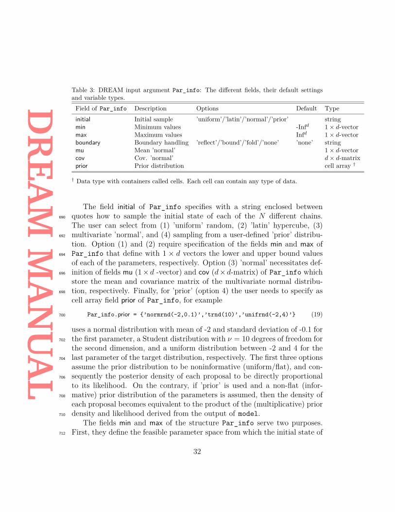
Table 3: DREAM input argument Par_info: The different fields, their default settingsand variable types.Field of Par_info Description Options Default Typeinitial Initial sample ’uniform’/’latin’/’normal’/’prior’ stringmin Minimum values -Infd 1× d-vectormax Maximum values Infd 1× d-vectorboundary Boundary handling ’reflect’/’bound’/’fold’/’none’ ’none’ stringmu Mean ’normal’ 1× d-vectorcov Cov. ’normal’ d× d-matrixprior Prior distribution cell array †
† Data type with containers called cells. Each cell can contain any type of data.
The field initial of Par_info specifies with a string enclosed betweenquotes how to sample the initial state of each of the N different chains.690
The user can select from (1) ’uniform’ random, (2) ’latin’ hypercube, (3)multivariate ’normal’, and (4) sampling from a user-defined ’prior’ distribu-692
tion. Option (1) and (2) require specification of the fields min and max ofPar_info that define with 1 × d vectors the lower and upper bound values694
of each of the parameters, respectively. Option (3) ’normal’ necessitates def-inition of fields mu (1× d -vector) and cov (d× d-matrix) of Par_info which696
store the mean and covariance matrix of the multivariate normal distribu-tion, respectively. Finally, for ’prior’ (option 4) the user needs to specify as698
cell array field prior of Par_info, for example
Par_info.prior = {’normrnd(-2,0.1)’,’trnd(10)’,’unifrnd(-2,4)’} (19)700
uses a normal distribution with mean of -2 and standard deviation of -0.1 forthe first parameter, a Student distribution with ν = 10 degrees of freedom for702
the second dimension, and a uniform distribution between -2 and 4 for thelast parameter of the target distribution, respectively. The first three options704
assume the prior distribution to be noninformative (uniform/flat), and con-sequently the posterior density of each proposal to be directly proportional706
to its likelihood. On the contrary, if ’prior’ is used and a non-flat (infor-mative) prior distribution of the parameters is assumed, then the density of708
each proposal becomes equivalent to the product of the (multiplicative) priordensity and likelihood derived from the output of model.710
The fields min and max of the structure Par_info serve two purposes.First, they define the feasible parameter space from which the initial state of712
32

DR
EAM
MA
NU
AL
each of the chains is drawn if ’uniform’ random or ’latin’ hypercube samplingis used. Second, they can define a bounded search domain for problems714
involving one or more parameters with known physical/conceptual ranges.This does however require the bound to be actively enforced during chain716
evolution. Indeed, proposals generated with Equations (16) and (17) can falloutside the hypercube defined by min and max even if the initial state of718
each chain are well within the feasible search space. The field boundary ofPar_info provides several options what to do if the parameters are outside720
their respective ranges. The four different options that are available are (1)’bound’, (2) ’reflect’, (3) ’fold’, and (4) ’none’ (default). These methods are722
illustrated graphically in Figure 7 and act on one parameter at a time.
x 1
x 2
‘bound’ ‘reflect’ ‘fold’
x 2
x 2
x 1 x 1
Figure 10: Different options for parameter boundary handling in the DREAM package, a)set to bound, b) reflection, and c) folding. The option folding is the only approach thatdoes not destroy the Markovian properties of the Markov chain.
The option ’bound’ is most simplistic and simply resets each dimension724
of the d-vector of parameters that is outside the bound equal to its respectivebound. The option ’reflect’ is somewhat more refined and views the bound-726
ary of the search space as a mirror through which individual dimensions arereflected backwards into the parameter space. The size of this reflection is728
set equal to the "amount" of boundary violation. The ’bound’ and ’reflect’boundary treatment options are used often in the field of optimization con-730
cerned with finding the global optimum of a given cost or objective function.Unfortunately, these two methods violate detailed balance in the context of732
MCMC simulation by introducing irreversible chain transitions. Indeed, the’bound’ or ’reflect’ correction step of the proposal modify the forward jump734
and the backward jump cannot be construed with equal probability. Thethird option ’fold’ connects the upper and lower bound of the parameter736
33
DR
EAM
MA
NU
AL
space so as to create a continuum representation. This approach is statis-tically preferred as it does not destroy the Markovian properties of the N738
sampled chains. However, this approach can give "bad" proposals if at leastone of the dimensions of the posterior distribution is located at the edges of740
the search domain. For those dimensions the parameter values can transitiondirectly from low to high values, and vice versa.742
Practical experience suggests that a reflection approach is most efficientand only slightly affects detailed balance of the sampled chains. The option744
’bound’ is least recommended as it can collapse the parameter values of agiven dimension to a single point, thereby not only loosing diversity for sam-746
pling but also inflating the probability mass at the bound. Other undesiredside-effects are the loss of chain diversity causing a-periodicity (proposal and748
current state are similar for selected dimensions) and distorting convergenceto the appropriate limiting distribution. A benchmark run with a truncated750
normal target distribution will demonstrate that folding gives exact resultswhereas a reflection step provides reasonable results.752
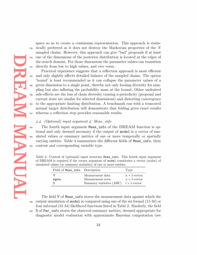
4.4. (Optional) input argument 4: Meas_infoThe fourth input argument Meas_info of the DREAM function is op-754
tional and only deemed necessary if the output of model is a vector of sim-ulated values or summary metrics of one or more temporally or spatially756
varying entities. Table 4 summarizes the different fields of Meas_info, theircontent and corresponding variable type.758
Table 4: Content of (optional) input structure Meas_info. This fourth input argumentof DREAM is required if the return argument of model constitutes a vector (scalar) ofsimulated values (or summary statistics) of one or more entities.
Field of Meas_info Description TypeY Measurement data n× 1-vectorsigma Measurement error n× 1-vectorS Summary statistics (ABC) l × 1-vector
The field Y of Meas_info stores the measurement data against which theoutput simulation of model is compared using one of the six formal (11-16) or760
four informal (31-34) likelihood functions listed in Table 2. Similarly, the fieldS of Par_info stores the observed summary metrics, deemed appropriate for762
diagnostic model evaluation with approximate Bayesian computation (see
34

DR
EAM
MA
NU
AL
next section) using likelihood function 21 or 22. The number of elements764
of Y and S should match exactly the output of model. The field sigma ofMeas_info allows the user to specify the measurement error of each value of766
Y, which constitutes necessary input for likelihood function 12, 13 and 16. Ifhomoscedasticity of the measurement data error is assumed then sigma can768
be defined a scalar, whereas a n × 1 vector of sigma values is appropriate ifheteroscedasticity of Y is expected.770
If the measurement error of the data is unknown then the user can selectlikelihood function 11, or alternatively infer the measurement error jointly772
with the parameters of the target distribution. An example of such approachis given in the script runDREAM of the MATLAB package and uses the774
generalized likelihood function (Schoups and Vrugt, 2010a) (likelihood func-tion 14). Alternatively, the user can specify sigma as an inline function,776
for example, Meas_info.sigma = inline(’a + bY’), where "a" and "b" areunknown variables that will be estimated along with the parameters. This778
formulation assumes the measurement error to be linearly dependent on theobserved data, and allows for homoscedasticity and heteroscedasticity. Infer-780
ence of "a" and "b" using likelihood 12, 13 or 16 will convey what measurementerror model is most appropriate. Joint inference does require the user to add782
the unknown variables "a" and "b" of the inline function to the parametervector. The ranges of "a" and "b" in the d + 2 row vectors, min and max784
should be carefully chosen so that sigma > 0 ∀ ”a”, ”b”.
4.5. (Optional) input argument 5: options786
The structure options is optional and passed as fifth input argumentto DREAM. The fields of this structure can activate (among others) file788
writing, distributed multi-core calculation, storage of model output, and di-agnostic model evaluation with approximate Bayesian computation. Table 5790
summarizes the different fields of options and their default settings.
35

DR
EAM
MA
NU
AL
Table 5: Content of (optional) input structure options. This fifth input argument ofDREAM is required to activate built-in functionalities such as distributed multi-processorcalculation, workspace saving, and diagnostic model evaluation with approximate Bayesiancomputation using DREAM(ABC)
Field of options Description Options Typeparallel Distributed multi-core calculation? no/yes stringIO If parallel, IO writing of model? no/yes stringmodout Store output of model? no/yes stringsave Save DREAM workspace? no/yes stringrestart Restart run? (’save’ required) no/yes stringABC Approximate Bayesian computation? no/yes stringepsilon ABC cutoff threshold scalar †rho ABC distance function inline function ‡
† Default setting of 0.025.‡ Default distance function is ’inline(’abs(Y-S)’)’
Multi-core calculation takes advantage of the MATLAB Parallel Comput-792
ing Toolbox and evaluates the N different proposals created with Equations(16) and (17) on a different processor. This is especially useful if the for-794
ward model, model is CPU-demanding and requires at least a few seconds(often more) to run. The field IO of options determines the setup of the796
distributed computing environment. If file writing is used to communicatebetween DREAM and an external executable called from model using the798
built-in dos or unix command, then each processor is setup automaticallyto work in a different directory. This is a simple solution to file overwriting800
and corruption that occurs if multiple different proposals are evaluated inthe same directory. If model consists of MATLAB code only with/without802
shared libraries linked through the built-in MEX-compiler then the parame-ter values, x can be passed directly to this .mex or .dll function and a single804
common directory for all workers suffices.For CPU-intensive forward models it is convenient to not only store the806
parameter samples but also keep in memory the corresponding model simula-tions returned by model and used to calculate the likelihood of each proposal.808
This avoids having to rerun the model script again after DREAM has termi-nated to assess posterior simulation uncertainty ranges. The field modout of810
options determines whether to store the output of the model script. If modeloutput writing is activated (’yes’) then the N simulations of X are stored812
in a binary file ’Z.bin’ after each generation. These simulations are then re-
36

DR
EAM
MA
NU
AL
turned to the user as third output argument, fx of DREAM. If thinning is814
activated then this applies to the simulations stored in fx as well.To help evaluate the progress of DREAM, it can be useful to periodically816
store the MATLAB workspace to a file. If the field save of options is setto ’yes’ then the workspace is saved to the file ’DREAM.mat’ after each818
successive iteration. This temporary file is necessary input for a restartrun (field restart) if convergence has not been achieved with the assumed820
computational budget.Finally, the field ABC of options enables diagnostic model evaluation822
using approximate Bayesian computation. This approach is designed specif-ically for cases when the output of model constitutes a vector of summary824
statistics rather than the original data, Y itself. If ABC is used, then thefields rho and epsilon of options need to be specified. The field rho defines826
with an inline function object the mathematical formulation of the distancefunction between the simulated and observed summary statistics. In practice,828
a simple difference operator rho = inline(’abs(Y-S)’) (set as default) of-ten suffices, where Y (output of model) and S (stored in field S of Meas_info)830
denote the observed and measured summary statistics, respectively. The fieldepsilon of options stores a small nominal value (default of 0.025) which is832
used to delineate the behavioral (posterior) samples.If ABC is used then the user can select two different implementations to834
solve for the target distribution. The first approach is adopted from Turnerand Sederberg (2012) and uses likelihood function 21 to transform the dis-836
tance function between the observed and simulated summary metrics in aprobability density that DREAM uses to derive the target distribution. This838
approach can produce nicely bell-shaped marginal distributions, but does notguarantee that the posterior summary metrics fall within epsilon of their ob-840
served values. A more viable and powerful approach was introduced recentlyby Sadegh and Vrugt (2014) and uses likelihood function 22 and a (two-stage)842
Metropolis acceptance probability to decide whether to accept proposals ornot. This new method, called DREAM(ABC) rapidly guides the posterior sum-844
mary metrics to lie within epsilon of their observed counterparts. Section 5of this paper demonstrates the application of ABC to diagnostic inference846
using an illustrative case study involving a catchment hydrologic model.
4.6. Output arguments848
We now briefly discuss the three output (return) arguments of DREAMincluding chain, output and fx. These three variables summarize the results850
37

DR
EAM
MA
NU
AL
of the DREAM algorithm and are used for convergence assessment, posterioranalysis and plotting.852
The variable chain is a matrix of size T×d+2×N . The first d columns ofchain store the sampled parameter values (state), whereas the subsequent854
two columns list the associated log-prior and log-likelihood values respec-tively. If thinning is applied to each of the Markov chains then the number856
of rows of chain is equivalent to T/K+1, where K ≥ 2 denotes the thinningrate. If a non-informative (uniform) prior is used then the values in column858
d + 1 of chain are all zero and consequently, p(θ|Y) ∝ L(θ|Y). With aninformative prior, the values in column d+ 1 are non-zero and the posterior860
density, p(θ|Y) ∝ p(θ)L(θ|Y).The following MATLAB command862
plot(chain(1:end,1,2),’r+’) (20)
creates a trace plot (using red dots) of the first parameter of the second864
chain. By plotting in the same figure the remaining N − 1 chains (usingdifferent colors/symbols), the mixing of the Markov chains can be assessed866
visually. This will help judge when convergence of the sampled trajectoriesto a limiting distribution has been achieved.868
The structure output contains important (diagnostic) information aboutthe progress of the DREAM algorithm. The field RunTime (scalar) stores870
the wall-time (seconds), R_stat (matrix), AR (matrix) and CR (matrix) listfor a given number of generations the R convergence diagnostic of Gelman872
and Rubin (1992) for each of the d parameters of the target distribution,the average acceptance rate and selection probabilities of each of the ncr874
crossover values, respectively, and outlier (vector) contains the index of alloutlier chains (often empty). Note that at the end of each DREAM trial, the876
autocorrelation function and Geweke (1992) and Raftery and Lewis (1992,1995) convergence diagnostics of each of the N chains and printed to the878
screen in the MATLAB editor.The MATLAB command880
plot(output.R_stat(1:end,2:DREAMPar.N+1)) (21)
plots with different colors the evolution of the R-convergence diagnostic of882
each parameter.Finally, the matrix fx stores the output Y of model. If this return argu-884
ment constitutes a vector of simulated values (summary metrics) then fx is
38

DR
EAM
MA
NU
AL
of size NT × n (NT × s), otherwise fx is a vector of NT × 1 with likelihood886
or log-likelihood values. If thinning is used then this applies to fx as welland the number of rows of fx becomes equivalent to T/K + 1;K ≥ 2.888
The directory ’../postprocessing’ (under main directory) contains a num-ber of different functions that can be used to visualize the different output890
arguments of DREAM. The script DREAM_postproc can be executed fromthe MATLAB prompt after the main DREAM function has terminated. Ap-892
pendix A summarizes briefly the graphical output of the post-processingscripts.894
5. Numerical examples
I now demonstrate the application of the MATLAB DREAM package to896
six different inference problems. These case studies cover a diverse set ofproblem features and involve (among others) bimodal and high-dimensional898
target distributions, summary statistics, dynamic simulation models, for-mal/informal likelihood functions, diagnostic model evaluation, Bayesian900
model averaging, and informative/noninformative prior parameter distribu-tions.902
5.1. Case Study I: one-dimensional mixture distributionWe revisit the bimodal target distribution of Equation 14. The modes at904
-8 and 10 are so far separated that it is notoriously difficult for regular covari-ance based proposal distributions (AM and RWM) to sample correctly the906
target distribution. The initial state of the chains is sampled from U [−20, 20].The following MATLAB script defines the problem setup.908
%% Problem settings defined by userDREAMPar.d = 1; % Dimension of the problemDREAMPar.N = 10; % Number of Markov chainsDREAMPar.T = 2500; % Number of generationsDREAMPar.lik = 1; % Model output is likelihood
%% Initial sampling and parameter rangesPar_info.initial = 'latin'; % Latin hypercube samplingPar_info.min = [ −20 ]; % Lower bound parametersPar_info.max = [ 20 ]; % Upper bound parameters
%% Define name of function (.m file) for posterior explorationFunc_name = 'mixture';
%% Run the DREAM algorithm[chain,output,fx] = DREAM(Func_name,DREAMPar,Par_info);
Figure 11: Case study I: Univariate mixture distribution consisting of two different modes.
39

DR
EAM
MA
NU
AL
The initial sample is drawn using Latin hypercube sampling, and thetarget distribution is defined in the script mixture of Appendix C. Figure910
12 plots a histogram of the posterior samples. The average acceptance rateis about 36.3%.912
−10 0 100
0.1
0.2
0.3
0.4
Den
sity
x
(A)
0 1,000 2,000 3,000 4,000 5,000−15
−5
5
15
(B)
x
Sample of Markov chain
Figure 12: (A) Histogram of posterior distribution derived from DREAM using N = 10chains, and T = 5, 000 generations. The solid black line depict the target distribution.(B) Trace plot. Individual chains are coded with a different color (symbol).
The sampled distribution is in excellent agreement with the target dis-tribution, in large part due to the ability of DREAM to jump directly from914
one mode to the other when γ = 1.
5.2. Case Study II: 100-dimensional t-distribution916
Our second case study involves a 100-dimensional Student distributionwith 60 degrees of freedom. The target distribution, defined in the script918
t_distribution of Appendix C, is centered at the zeroth vector, with allpairwise correlations equivalent to 0.5.920
40
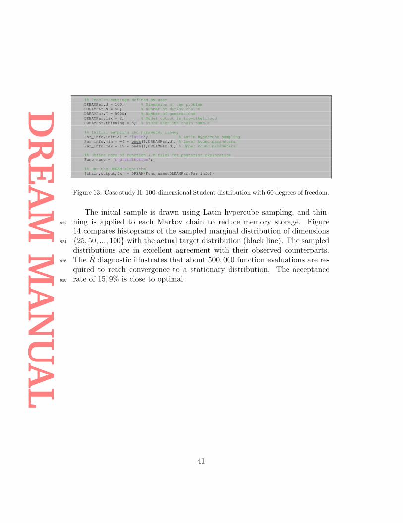
DR
EAM
MA
NU
AL
%% Problem settings defined by userDREAMPar.d = 100; % Dimension of the problemDREAMPar.N = 50; % Number of Markov chainsDREAMPar.T = 5000; % Number of generationsDREAMPar.lik = 2; % Model output is log−likelihoodDREAMPar.thinning = 5; % Store each 5th chain sample
%% Initial sampling and parameter rangesPar_info.initial = 'latin'; % Latin hypercube samplingPar_info.min = −5 * ones(1,DREAMPar.d); % Lower bound parametersPar_info.max = 15 * ones(1,DREAMPar.d); % Upper bound parameters
%% Define name of function (.m file) for posterior explorationFunc_name = 't_distribution';
%% Run the DREAM algorithm[chain,output,fx] = DREAM(Func_name,DREAMPar,Par_info);
Figure 13: Case study II: 100-dimensional Student distribution with 60 degrees of freedom.
The initial sample is drawn using Latin hypercube sampling, and thin-ning is applied to each Markov chain to reduce memory storage. Figure922
14 compares histograms of the sampled marginal distribution of dimensions{25, 50, ..., 100} with the actual target distribution (black line). The sampled924
distributions are in excellent agreement with their observed counterparts.The R diagnostic illustrates that about 500, 000 function evaluations are re-926
quired to reach convergence to a stationary distribution. The acceptancerate of 15, 9% is close to optimal.928
41
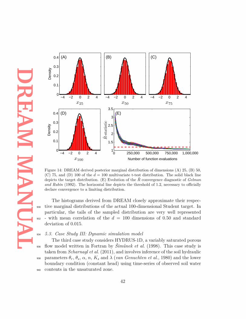
DR
EAM
MA
NU
AL
−4 −2 0 2 40
0.1
0.2
0.3
0.4
Den
sity
(A)
x25
−4 −2 0 2 4
(B)
x50
−4 −2 0 2 4
(C)
x75
−4 −2 0 2 4 0
0.1
0.2
0.3
0.4 (D)
x100
Den
sity
0 250,000 500,000 750,000 1,000,0001
1.5
2
2.5
3
3.5(E)
Number of function evaluations
R-statistic
Figure 14: DREAM derived posterior marginal distribution of dimensions (A) 25, (B) 50,(C) 75, and (D) 100 of the d = 100 multivariate t-test distribution. The solid black linedepicts the target distribution. (E) Evolution of the R convergence diagnostic of Gelmanand Rubin (1992). The horizontal line depicts the threshold of 1.2, necessary to officiallydeclare convergence to a limiting distribution.
The histograms derived from DREAM closely approximate their respec-tive marginal distributions of the actual 100-dimensional Student target. In930
particular, the tails of the sampled distribution are very well represented- with mean correlation of the d = 100 dimensions of 0.50 and standard932
deviation of 0.015.
5.3. Case Study III: Dynamic simulation model934
The third case study considers HYDRUS-1D, a variably saturated porousflow model written in Fortran by Šimůnek et al. (1998). This case study is936
taken from Scharnagl et al. (2011), and involves inference of the soil hydraulicparameters θr, θs, α, n, Ks and λ (van Genuchten et al., 1980) and the lower938
boundary condition (constant head) using time-series of observed soil watercontents in the unsaturated zone.940
42
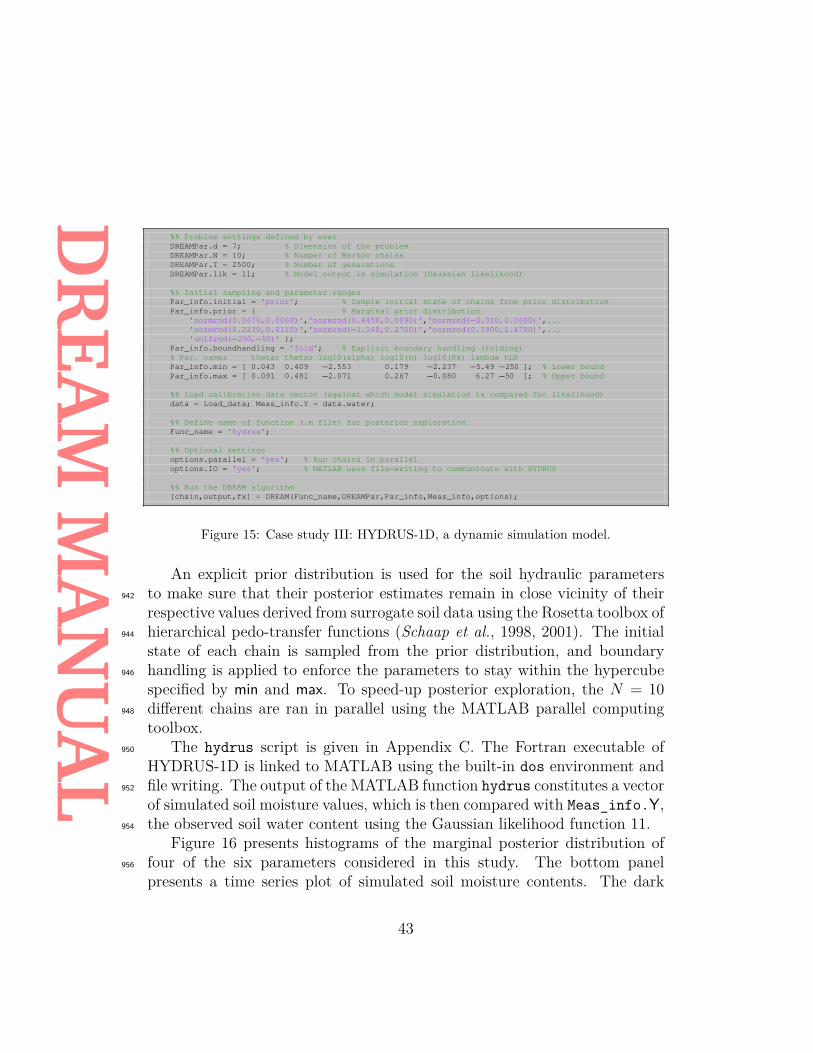
DR
EAM
MA
NU
AL
%% Problem settings defined by userDREAMPar.d = 7; % Dimension of the problemDREAMPar.N = 10; % Number of Markov chainsDREAMPar.T = 2500; % Number of generationsDREAMPar.lik = 11; % Model output is simulation (Gaussian likelihood)
%% Initial sampling and parameter rangesPar_info.initial = 'prior'; % Sample initial state of chains from prior distributionPar_info.prior = { % Marginal prior distribution
'normrnd(0.0670,0.0060)','normrnd(0.4450,0.0090)','normrnd(−2.310,0.0600)',...'normrnd(0.2230,0.0110)','normrnd(−1.160,0.2700)','normrnd(0.3900,1.4700)',...'unifrnd(−250,−50)' };
Par_info.boundhandling = 'fold'; % Explicit boundary handling (folding)% Par. names thetar thetas log10(alpha) log10(n) log10(Ks) lambda hLBPar_info.min = [ 0.043 0.409 −2.553 0.179 −2.237 −5.49 −250 ]; % Lower boundPar_info.max = [ 0.091 0.481 −2.071 0.267 −0.080 6.27 −50 ]; % Upper bound
%% Load calibration data vector (against which model simulation is compared for likelihood)data = Load_data; Meas_info.Y = data.water;
%% Define name of function (.m file) for posterior explorationFunc_name = 'hydrus';
%% Optional settingsoptions.parallel = 'yes'; % Run chains in paralleloptions.IO = 'yes'; % MATLAB uses file−writing to communicate with HYDRUS
%% Run the DREAM algorithm[chain,output,fx] = DREAM(Func_name,DREAMPar,Par_info,Meas_info,options);
Figure 15: Case study III: HYDRUS-1D, a dynamic simulation model.
An explicit prior distribution is used for the soil hydraulic parametersto make sure that their posterior estimates remain in close vicinity of their942
respective values derived from surrogate soil data using the Rosetta toolbox ofhierarchical pedo-transfer functions (Schaap et al., 1998, 2001). The initial944
state of each chain is sampled from the prior distribution, and boundaryhandling is applied to enforce the parameters to stay within the hypercube946
specified by min and max. To speed-up posterior exploration, the N = 10different chains are ran in parallel using the MATLAB parallel computing948
toolbox.The hydrus script is given in Appendix C. The Fortran executable of950
HYDRUS-1D is linked to MATLAB using the built-in dos environment andfile writing. The output of the MATLAB function hydrus constitutes a vector952
of simulated soil moisture values, which is then compared with Meas_info.Y,the observed soil water content using the Gaussian likelihood function 11.954
Figure 16 presents histograms of the marginal posterior distribution offour of the six parameters considered in this study. The bottom panel956
presents a time series plot of simulated soil moisture contents. The dark
43

DR
EAM
MA
NU
AL
gray region constitutes the 95% HYDRUS-1D simulation uncertainty due to958
parameter uncertainty, whereas the light gray region denotes total simula-tion uncertainty. The observed soil moisture values are indicated with a red960
circle.
0.43 0.45 0.47
0.2
0.4
0.6
0.8
1
θs (-)
(A)
Den
sity
0.003 0.005 0.007alpha (1/cm)
(B)
1.6 1.7 1.8n (-)
(C)
1 2 3 4 5Ks (cm/day)
(D)
80 100 120 140 160 180 200 220 240 260 2800.2
0.25
0.3
0.35
0.4
day of year
Soi
l moi
stur
e co
nten
t (cm
3 /cm
3 )
(E) total uncertainty
parameter uncertaintyobservations
Figure 16: Top panel: Histograms of marginal posterior distribution of the soil hydraulicparameters (A) θs, (B) α, (C) n, and (D) Ks. The prior distribution is indicated with asolid black line. (E) HYDRUS-1D 95% simulation uncertainty intervals due to parameter(dark region) and total uncertainty (light gray). The observed soil moisture value areindicated with a red circle.
The HYDRUS-1D model closely tracks the observed soil moisture con-962
tents with Root Mean Square Error (RMSE) of the posterior mean simulationof about 0.01 cm3/cm−3. About 95% of the observations lies within the gray964
region, an indication that the simulation uncertainty ranges are statisticallyadequate. The acceptance rate of DREAM averages about 12.6% - about966
half of its theoretical optimal value of 22-25% (for Gaussian and t- targets).This deficiency is caused by the numerical solver used to integrate Richards’968
equation.
44

DR
EAM
MA
NU
AL
5.4. Case Study IV: Diagnostic model evaluation970
The fourth case study illustrates the ability of DREAM to be used fordiagnostic model evaluation. We use a rather parsimonious 7-parameter972
lumped watershed model (also known as hmodel) using historical data fromthe Guadalupe River at Spring Branch, Texas. This is the driest of the 12974
MOPEX basins described in the study of Duan et al. (2006). The modelstructure and hydrologic process representations are found in Schoups and976
Vrugt (2010a). The model transforms rainfall into runoff at the watershedoutlet using explicit process descriptions of interception, throughfall, evapo-978
ration, runoff generation, percolation, and surface and subsurface routing.Daily discharge, mean areal precipitation, and mean areal potential evap-980
otranspiration were derived from Duan et al. (2006) and used for diagnos-tic model evaluation with DREAM(ABC) (Sadegh and Vrugt, 2014). Details982
about the basin and experimental data, and likelihood function can be foundthere, and will not be discussed herein. The same model and data was used984
in a previous study Schoups and Vrugt (2010a), and used to introduce thegeneralized likelihood function of Table 1.986
Four different summary metrics of the discharge data are used for ABCinference, including S1 (-) the annual runoff coefficient, S2 (-) the annual988
baseflow coefficient, and S3 (day/mm) and S4 (-) two coefficients of the flowduration curve (Vrugt and Sadegh, 2013; Sadegh et al., 2015). The following990
setup is used in the MATLAB package of DREAM.
45
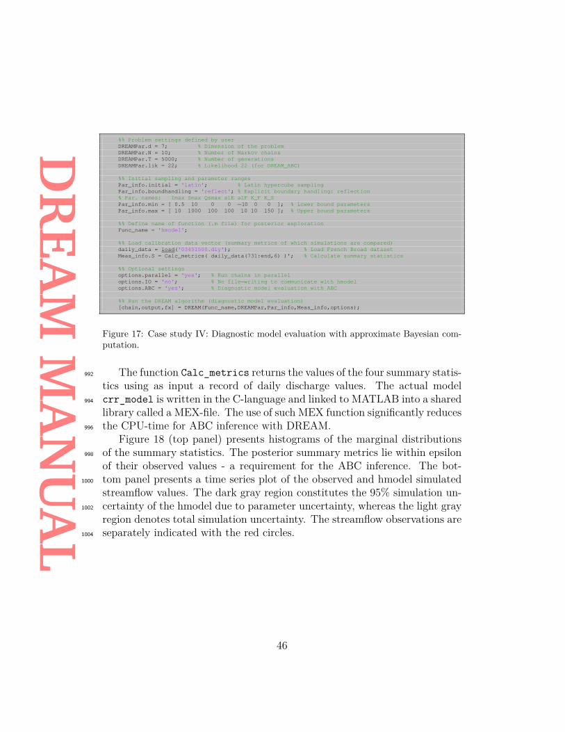
DR
EAM
MA
NU
AL
%% Problem settings defined by userDREAMPar.d = 7; % Dimension of the problemDREAMPar.N = 10; % Number of Markov chainsDREAMPar.T = 5000; % Number of generationsDREAMPar.lik = 22; % Likelihood 22 (for DREAM_ABC)
%% Initial sampling and parameter rangesPar_info.initial = 'latin'; % Latin hypercube samplingPar_info.boundhandling = 'reflect'; % Explicit boundary handling: reflection% Par. names: Imax Smax Qsmax alE alF K_F K_SPar_info.min = [ 0.5 10 0 0 −10 0 0 ]; % Lower bound parametersPar_info.max = [ 10 1000 100 100 10 10 150 ]; % Upper bound parameters
%% Define name of function (.m file) for posterior explorationFunc_name = 'hmodel';
%% Load calibration data vector (summary metrics of which simulations are compared)daily_data = load('03451500.dly'); % Load French Broad datasetMeas_info.S = Calc_metrics( daily_data(731:end,6) )'; % Calculate summary statistics
%% Optional settingsoptions.parallel = 'yes'; % Run chains in paralleloptions.IO = 'no'; % No file−writing to communicate with hmodeloptions.ABC = 'yes'; % Diagnostic model evaluation with ABC
%% Run the DREAM algorithm (diagnostic model evaluation)[chain,output,fx] = DREAM(Func_name,DREAMPar,Par_info,Meas_info,options);
Figure 17: Case study IV: Diagnostic model evaluation with approximate Bayesian com-putation.
The function Calc_metrics returns the values of the four summary statis-992
tics using as input a record of daily discharge values. The actual modelcrr_model is written in the C-language and linked to MATLAB into a shared994
library called a MEX-file. The use of such MEX function significantly reducesthe CPU-time for ABC inference with DREAM.996
Figure 18 (top panel) presents histograms of the marginal distributionsof the summary statistics. The posterior summary metrics lie within epsilon998
of their observed values - a requirement for the ABC inference. The bot-tom panel presents a time series plot of the observed and hmodel simulated1000
streamflow values. The dark gray region constitutes the 95% simulation un-certainty of the hmodel due to parameter uncertainty, whereas the light gray1002
region denotes total simulation uncertainty. The streamflow observations areseparately indicated with the red circles.1004
46

DR
EAM
MA
NU
AL
800 850 900 950 1,000 1,050 1,1000
10
20
30
day of year
Dis
ch
arg
e (
mm
/da
y)
(E)parameter uncertainty
observations
0.46 0.48 0.5
0.2
0.4
0.6
0.8
1
De
nsity
(A)
0.76 0.78 0.8
(B)
0.72 0.74 0.76
(C)
3.32 3.34 3.36
(D)
Figure 18: Application of DREAM(ABC) to the hmodel using historical data from theGuadalupe River at Spring Branch, Texas. Posterior marginal distribution of the summarymetrics (A) S1 (runoff coefficient), (B) S2 (baseflow index), (C) S3 and (D) S4 (twocoefficients of the flow duration curve). The blue vertical lines are epsilon removed fromthe observed summary metrics (blue cross) and delineate the behavioral (posterior) modelspace. The bottom panel (E) presents the 95% simulation uncertainty ranges of the hmodelfor a selected 300-day portion of the calibration data set. The observed discharge data areindicated with red circles.
The simulated summary metrics cluster closely (within epsilon) aroundtheir observed counterparts. About 15, 000 function evaluations were re-1006
quired with DREAM(ABC) to converge to a limiting distribution (not shown).This is orders of magnitude more efficient than commonly used rejection sam-1008
plers (Sadegh and Vrugt, 2014). Note that the hmodel nicely mimics the ob-served discharge dynamics with simulation uncertainty ranges that envelop a1010
large portion of the discharge observations. Thus, the four summary metricsused herein contain sufficient information to provide a reasonably adequate1012
calibration. We refer the interested reader to Vrugt and Sadegh (2013) andVrugt and Sadegh (2015) who present a much more detailed ABC analysis -1014
with particular focus on diagnosis and detection of epistemic errors.
47
DR
EAM
MA
NU
AL
5.5. Case Study V: Bayesian Model Averaging1016
Ensemble Bayesian Model Averaging (BMA) proposed by Raftery et al.(2005) is a widely used method for statistical post-processing of forecasts1018
from an ensemble of different models. The BMA predictive distribution ofany future quantity of interest is a weighted average of probability density1020
functions centered on the bias-corrected forecasts from a set of individualmodels. The weights are the estimated posterior model probabilities, repre-1022
senting each model’s relative forecast skill in the training (calibration) period.Successful application of BMA requires estimates of the weights and vari-1024
ances of the individual competing models in the ensemble. In their seminalpaper, Raftery et al. (2005) recommends using the Expectation Maximiza-1026
tion (EM) algorithm (Dempster et al., 1997). This method is relatively easyto implement, computationally efficient, but does not provide uncertainty es-1028
timates of the weights and variances. Here we demonstrate the application ofDREAM to BMA model training using a 36-year record of daily streamflow1030
observations from the Leaf River basin in the USA. An ensemble of eight dif-ferent watershed models is used in our analysis. The names of these models1032
and the RMSE (m3/s) of their forecast error are listed in Table 6.Theory, concepts and applications of DREAM(BMA) have been presented1034
by Vrugt et al. (2008c) and interested readers are referred to this publicationfor further details. Here, we restrict our attention to the setup of BMA in1036
the MATLAB package of DREAM.
48

DR
EAM
MA
NU
AL
%% Problem settings defined by userDREAMPar.T = 5000; % Number of generationsDREAMPar.lik = 2; % Model returns log−likelihood
%% Initial sampling and parameter rangesPar_info.initial = 'latin'; % Latin hypercube samplingPar_info.boundhandling = 'reflect'; % Explicit boundary handling
%% Define BMA as a global variableglobal BMA
%% Define name of function (.m file) for posterior explorationFunc_name = 'BMA_calc';
%% Load data from Vrugt and Robinson, WRR, 43, W01411, doi:10.1029/2005WR004838, 2007load data.txt; % Daily streamflow simulations eight watershed modelsload Y.txt; % Daily streamflow observationsStartT = 1; EndT = 3000; % Start/End day training periodBMA.PDF = 'gamma'; % pdf predictor: normal/heteroscedastic/gammaBMA.VAR = 'multiple'; % variance pdf: single/multiple (multiple for 'normal')
%% Setup the BMA model (apply linear bias correction)[DREAMPar,BMA,Par_info] = Setup_BMA(DREAMPar,Par_info,BMA,data,Y,StartT,EndT);
%% Run the DREAM algorithm[chain,output,fx] = DREAM(Func_name,DREAMPar,Par_info);
Figure 19: Case study V: Bayesian model averaging using MCMC simulation withDREAM.
The predictive distribution of each constituent member of the ensemble1038
is assumed to follow a gamma distribution with unknown heteroscedasticvariance. The BMA_calc script is listed in Appendix C.1040
Table 6 summarizes the results of DREAM(BMA) and presents (in column"Gamma") the maximum a-posteriori (MAP) values of the BMA weights for1042
the different models of the ensemble. Values listed in parentheses denotethe posterior standard deviation derived from the DREAM sample. We also1044
summarize the MAP values of the weights for a Gaussian (conditional) dis-tribution (columns "Normal") with homoscedastic (left) or heteroscedastic1046
(right) error variance, and report the average RMSE (m3/s), coverage (%)and spread (m3/s) of the resulting BMA model during the 26-year evaluation1048
period.
49

DR
EAM
MA
NU
AL
Table 6: Results of DREAM(BMA) by application to eight different watershed modelsusing daily discharge data from the Leaf River in Mississippi, USA. We list the individualforecast errors of the models for the training data period, the corresponding MAP valuesof the weights for a Gamma (default) and Gaussian forecast distribution, and presentthe results of the BMA model (bottom panel) during the evaluation period. The spread(m3/s) and coverage (%) are derived from a 95% prediction interval.Model RMSE Gamma Normal † Normal ‡
ABC 31.67 0.02 (0.006) 0.03 (0.010) 0.00 (0.002)GR4J 19.21 0.21 (0.016) 0.14 (0.013) 0.10 (0.013)HYMOD 19.03 0.03 (0.008) 0.13 (0.046) 0.00 (0.005)TOPMO 17.68 0.03 (0.006) 0.08 (0.047) 0.03 (0.010)AWBM 26.31 0.05 (0.009) 0.01 (0.010) 0.00 (0.002)NAM 20.22 0.05 (0.011) 0.14 (0.048) 0.11 (0.014)HBV 19.44 0.24 (0.017) 0.13 (0.034) 0.31 (0.016)SACSMA 16.45 0.37 (0.017) 0.34 (0.022) 0.43 (0.017)BMA: log-likelihood -9,775.1 -9,950.5 -9,189.4BMA: RMSE 22.54 23.22 23.16BMA: Spread 39.74 46.98 46.54BMA: Coverage 93.65% 92.59% 95.71%
† Homoscedastic (fixed) variance.‡ Heteroscedastic variance.
The values of the weights depend somewhat on the assumed conditional1050
distribution of the deterministic model forecasts of the ensemble. The GR4J,HBV and SACSMA models consistently receive the highest weights and are1052
thus most important in BMA model construction for this data set. Note alsothat TOPMO receives a very low BMA weight, despite it having the second1054
lowest RMSE value of the training data period. Correlation between theindividual forecasts of the watershed models affects strongly the posterior1056
distribution of the BMA weights. The gamma distribution is preferred forprobabilistic streamflow forecasting with 95% simulation uncertainty ranges1058
that, on average, are noticeably smaller than their counterparts derived froma normal distribution. We refer interested readers to Vrugt and Robinson1060
(2007a) and Rings et al. (2012) for a more detailed analysis of the BMAresults, and a comparison with filtering methods.1062
Figure 20 presents histograms of the marginal posterior distribution ofthe BMA weights for each of the models of the ensemble. The MAP values1064
of the weights are separately indicated with a blue cross.
50

DR
EAM
MA
NU
AL
0.01 0.03 0.05
0.2
0.4
0.6
0.8
1
De
nsity
(A) ABC
0.15 0.2 0.25
(B) GR4J
0.02 0.04 0.06
(C) HYMOD
0 0.02 0.04
(D) TOPMO
0.04 0.07 0.1
0.2
0.4
0.6
0.8
1
De
nsity
(E) AWBM
0.03 0.06 0.09
(F) NAM
0.2 0.25 0.3
(G) HBV
0.32 0.36 0.4
(H) SACSMA
Figure 20: Histograms of the marginal posterior distribution of the weights and variancesof each individual model of the ensemble. The MAP values of the weights are denotedwith a blue cross.
The distributions appear rather well-defined and exhibit an approximate1066
Gaussian shape. Analysis of the posterior weights helps to understand whichmodels of the ensemble are parameter uncertainty can be used to assess BMA1068
model uncertainty.
5.6. Case Study VI: Generalized Likelihood Uncertainty Estimation1070
Our sixth and last case study reports on GLUE and involves application ofan informal likelihood function to the study of animal population dynamics.1072
One of the first models to explain the interactions between predators andprey was proposed in 1925 by the American biophysicist Alfred Lotka and1074
the Italian mathematician Vito Volterra. This model, one of the earliest intheoretical ecology, has been widely used to study population dynamics, and1076
is given by the following system of two coupled differential equations
dP 1t
dt= αP 1
t − βP 1t P
2t1078
dP 2t
dt= −γP 2
t + δP 1t P
2t , (22)
1080
51

DR
EAM
MA
NU
AL
where P 1t and P 2
t denote the size of the prey and predator population attime t respectively, α (-) is the prey growth rate (assumed exponential in1082
the absence of any predators), β (-) signifies the attack rate (prey mortalityrate for per-capita predation), γ (-) represents the exponential death rate for1084
predators in the absence of any prey, and δ (-) is the efficiency of conversionfrom prey to predator.1086
A synthetic monthly data set of a prey and predator population is createdby solving Equation (22) numerically for a 20-year period using an implicit,1088
time-variable, integration method (built-in ode solver). The initial states,P 1
0 = 30 and P 20 = 4 and parameter values α = 0.5471, β = 0.0281, γ =1090
0.8439 and δ = 0.0266 correspond to data collected by the Hudson BayCompany between 1900 and 1920. These synthetic monthly observations are1092
subsequently perturbed with a homoscedastic error, and this corrupted dataset is saved as text file ’abundances.txt’ and used for inference. The following1094
setup of DREAM is used in MATLAB.
%% Problem settings defined by userDREAMPar.d = 4; % Dimension of the problemDREAMPar.N = 10; % Number of Markov chainsDREAMPar.T = 2500; % Number of generationsDREAMPar.lik = 32; % Informal likelihood functionDREAMPar.GLUE = 10; % Value of likelihood shape parameter (for GLUE)
%% Initial sampling and parameter rangesPar_info.initial = 'latin'; % Latin hypercube samplingPar_info.boundhandling = 'reflect'; % Explicit boundary handling: reflection% Par. names: alpha beta gamma deltaPar_info.min = [ 0 0 0 0 ]; % Lower bound parametersPar_info.max = [ 1 10 1 10 ]; % Upper bound parameters
%% Load calibration data vectorMeas_info.Y = load('abundances.txt'); % Load food web dataset
%% Define name of function (.m file) for posterior explorationFunc_name = 'lotka_volterra';
%% Optional settingsoptions.parallel = 'yes'; % Run chains in paralleloptions.modout = 'yes'; % Store model simulations
%% Run the DREAM algorithm (diagnostic model evaluation)[chain,output,fx] = DREAM(Func_name,DREAMPar,Par_info,Meas_info,options);
Figure 21: Case study VI: Population dynamics using Lotka Volterra predator-prey model.
An informal likelihood function (31) is used to transform the difference1096
between the observed and simulated predator-prey populations in a likeli-hood. The forward model script lotka_volterra can be found in Appendix1098
C.Figure 22 presents the marginal posterior distributions of the parameters1100
α, β, γ and δ (top panel) and displays (bottom panel) the 95% uncertainty
52

DR
EAM
MA
NU
AL
(dark grey) of the simulated prey and predator populations. The observed1102
species abundances are separately indicated with the red circles.
0.3 0.6 0.9
0.2
0.4
0.6
0.8
1
Den
sity
α (-)
(A)
0 0.1 0.2
β (-)
(B)
0.3 0.6 0.9
γ (-)
(C)
0.02 0.05 0.08
δ (-)
(D)
0 4 8 12 16 200
25
50
75
100
year
Pre
y po
pula
tion
(E)
0 4 8 12 16 200
20
40
60
80(F)
year
Pre
dato
r po
pula
tion
Figure 22: Histograms (top panel) of the marginal posterior distribution of the Lotka-Volterra model parameters (A) α, (B) β, (C) γ, and (D) δ. Time series plot (bottompanel) of 95% simulation uncertainty ranges of the (E) prey and (F) predator populations.The observed data are indicated with the red circles.
The parameter δ appears best defined by calibration against the observed1104
species abundances with posterior ranges that are rather tight. The his-tograms of α and γ are rather disperse with posterior ranges that encompass1106
a large part of the prior distribution. This relatively large parameter uncer-tainty translates into an unrealistically large prediction uncertainty (bottom1108
panel). Of course, the results of DREAM depend strongly on the value of theshaping factor, GLUE of DREAMPar in likelihood function 32. If this value is1110
taken to be much larger (e.g. 100), then the marginal distributions would bemuch peakier and center on the "true" Lokta-Volterra parameter values used1112
to generate the synthetic record of predator and prey populations. Moreover,the spread of the 95% prediction uncertainty would be much smaller. We1114
refer the reader to Blasone et al. (2008) who illustrates in much more depththe application of MCMC simulation to GLUE inference.1116
53

DR
EAM
MA
NU
AL
6. Additional options
The six case studies presented herein illustrate only some of the main1118
capabilities of the DREAM software package. Yet, not all the options, dis-cussed initially in the presentation of the toolbox have been demonstrated1120
explicitly. The script runDREAM presents an exhaustive overview of thedifferent options and capabilities of the DREAM software suite, and includes1122
20 examples involving inference of much more complex and higher dimen-sional target distributions as well, for example estimation of the two- and/or1124
three-dimensional soil moisture distribution from travel time data of groundpenetrating radar (Laloy et al., 2012b; Linde and Vrugt, 2013) and treatment1126
of rainfall uncertainty in hydrologic modeling (Vrugt et al., 2008a). Users candraw from the different test problems and use them as templates for their1128
own modeling problems.I list a few other topics that can be integrated within DREAM.1130
(I) Copula’s. A copula is a multivariate probability distribution for whichthe marginal probability distribution of each variable is uniform. They1132
are used widely to describe the dependence between two or more ran-dom variables, for instance temperature and precipitation. This in-1134
cludes regular Archimedean and maximum entropy based copulae (Zhangand Singh, 2012; Aghakouchak, 2014).1136
(II) Diagnostic Bayes. A recurrent issue with the application of ABC is self-sufficiency of the summary statistics. In theory, S(·) should contain as1138
much information as the original data itself, yet complex systems rarelyadmit sufficient statistics. therefore proposed in another recent article1140
(Vrugt and Sadegh, 2015) a hybrid approach, coined diagnostic Bayes,that uses the summary metrics as prior distribution and the original1142
data in the likelihood function, or p(x|Y) ∝ p(x|S(Y))L(x|Y). Thismethod guarantees that no information is lost during the inference and1144
a posterior sample which adequately portrays the observed signaturesof system behavior1146
(III) Joint parameter and state estimation. If the function script modelimplements state estimation for some model, F(x, ) and assumed pa-1148
rameter vector, x (input argument) then DREAM can be used to derivethe posterior parameter distribution. If the return argument of model1150
is the mean ensemble model forecast then this constitutes the SODAframework of Vrugt et al. (2005), whereas if the marginal likelihood of1152
54
DR
EAM
MA
NU
AL
the state trajectories is returned then this approach is equivalent toParticle-DREAM (Vrugt et al., 2013).1154
(IV) Model selection. Bayes Law states that p(H|Y) = p(H)L(H|Y)/p(Y),where p(Y) acts as normalization constant so that the posterior distri-1156
bution is a proper probability density function,∫H p(H)L(H|Y)dH = 1
(see also Equation 4). The value of p(Y) can be estimated from multi-1158
dimensional numerical integration of the posterior distribution (Volpiet al., 2015) - the computer code of which is integrated in DREAM.1160
Knowledge of p(Y) (also called evidence) is required for (Bayesian)model selection. Indeed, the hypothesis (model) with the largest value1162
of p(Y) for a given data set is preferred statistically.
Most applications of Bayesian inference in the Earth sciences conveniently1164
assume the model to be a perfect representation of reality, the input (forcing)data to be observed without error, and consequently the parameters to be the1166
only source of uncertainty. The assumption of a perfect model and input datais not particularly realistic. We can relax this assumption, p(F(x, ·)|Y) ∝1168
p(x)L(F(x, ·)|H) and use latent variables to treat explicitly errors in themodel, F and input data, ·. The latent variables are then subject to inference1170
along with the parameters of the model.
7. DREAM: Related algorithms1172
In the past years, several other variants of DREAM have been developedto permit inference of discrete and combinatorial search problems, and en-1174
hance efficiency for high-dimensional and CPU-intensive system models. Ibriefly summarize these different algorithms1176
1 DREAM(ZS): This algorithm calculates the jump in Equation 16 froman archive of past states of the chains rather than the current states1178
of the N chains. This modification allows for the use of a much lowernumber of chains, yet turns the method into an adaptive Metropolis1180
sampler (ter Braak and Vrugt, 2008). Benchmark experiments demon-strate that N = 3 is sufficient for a large range of target dimensionali-1182
ties.2 DREAM(D): This code is especially developed for non-continuous, dis-1184
crete, and combinatorial target distributions. This algorithm uses
55

DR
EAM
MA
NU
AL
DREAM as its main building block and implements two novel pro-1186
posal distributions to explicitly recognize differences in topology be-tween discrete and Euclidean search spaces. The DREAM(D) sampler1188
is designed especially to solve experimental design problems involvingreal-time selection of measurements that discriminate best among mul-1190
tiple different hypothesis (models) of the system of interest (Vrugt etal., 2011; Kikuchi et al., 2015).1192
3 DREAM(DZS): Alternative variant of DREAM(D) that uses samplingfrom an archive of past states to generate proposal points in each of1194
the chains.4 MT-DREAM(ZS): This code is developed specifically for distributed1196
multi-core calculation of parameter rich CPU-intensive system modelsand merges multiple-try sampling (Liu et al., 2000), snooker updating,1198
and sampling from an archive of past states. Benchmark experiments ingeophysics, hydrology and hydrogeology have shown that this sampler1200
is able to sample correctly high-dimensional target distributions (Laloyand Vrugt, 2012a; Laloy et al., 2012b, 2013; Linde and Vrugt, 2013;1202
Carbajal et al., 2014; Lochbühler et al., 2014, 2015).A MATLAB toolbox, similar to the one presented herein for DREAM, is1204
available for each of these four algorithms, including multi-criteria optimiza-tion with AMALGAM (Vrugt and Robinson, 2007b).1206
8. Summary
In this paper I have reviewed the basic theory of Markov chain Monte1208
Carlo (MCMC) simulation and have introduced a MATLAB package of theDREAM algorithm. This toolbox provides scientists and engineers with an1210
arsenal of options and utilities to solve posterior sampling problems involv-ing (amongst others) bimodality, high-dimensionality, summary statistics,1212
bounded parameter spaces, dynamic simulation models, formal/informal like-lihood functions, diagnostic model evaluation, data assimilation, Bayesian1214
model averaging, distributed computation, and informative/noninformativeprior distributions. The DREAM toolbox supports parallel computing and1216
includes tools for convergence analysis of the sampled chain trajectories andpost-processing of the results. Six different case studies were used to il-1218
lustrate the main capabilities and functionalities of the MATLAB toolbox.These example studies are easy to run and adapt and serve as templates for1220
other inference problems.
56

DR
EAM
MA
NU
AL
A graphical user interface (GUI) of DREAM is currently under develop-1222
ment and will become available in due course.
9. Acknowledgements1224
The MATLAB toolbox of DREAM is available upon request from thefirst author, [email protected]. [Template: The comments of the anonymous1226
referees are greatly appreciated].
57

DR
EAM
MA
NU
AL
10. Appendix A1228
Table 7 summarizes, in alphabetic order, the different function/programfiles of the DREAM package in MATLAB. The main program runDREAM1230
contains seventeen different prototype studies which cover a large range ofproblem features. These example studies have been published in the geo-1232
physics, hydrologic, pedometrics, statistics and vadose zone literature, andprovide a template for users to setup their own case study. The last line1234
of each example study involves a function call to DREAM, which uses allthe other functions listed below to generate samples of the posterior dis-1236
tribution. Each example problem of runDREAM has its own directorywhich stores the model script written by the user and all other files (data1238
file(s), MATLAB scripts, external executable(s), etc.) necessary to computethe density/likelihood/log-likelihood/simulation/summary statistics of each1240
proposal.At the end of each DREAM trial, the autocorrelation function, Geweke1242
(1992) and Raftery and Lewis (1992, 1995) convergence diagnostic are com-puted separately for each of the N chains using the CODA toolbox written1244
by James P. LeSage (http://www.spatial-econometrics.com/). Thesefunctions are stored in the directory ’../diagnostics’ and produce a text file1246
’DREAM_diagnostics.txt’ that is printed to the screen at the end of sam-pling using the MATLAB editor. These three convergence diagnostics are1248
designed specifically for single-chain Metropolis samplers, and augment themulti-chain R statistic of Gelman and Rubin (1992) stored in the field R_stat1250
of output. Altogether, these four diagnostics should help to judge after howmany iterations (generations) the chains have converged to a limiting dis-1252
tribution. The subsequent samples can then be used to approximate theposterior distribution. In practice, I recommend as well to verify conver-1254
gence by visually inspecting the mixing of the different chain trajectories.Note that the CODA functions require each chain to have at least 200 sam-1256
ples otherwise the single-chain diagnostics cannot be computed (unstable)and the file ’DREAM_diagnostics.txt’ is empty.1258
The directory ’../postprocessing’ contains a number of different functionsdesigned to visualize the results (output arguments) of DREAM. The pro-1260
gram DREAM_postproc creates a large number of MATLAB figures,including trace plots of the sampled chain trajectories, bivariate scatter plots1262
and histograms of the posterior samples, a trace plot of the R-diagnostic, au-tocorrelation functions of the sampled parameter values, a quantile-quantile1264
58

DR
EAM
MA
NU
AL
Table7:
Descriptio
nof
theMAT
LAB
func
tions
andscrip
ts(.m
files)used
byDREA
M,v
ersio
n3.0.
Nam
eof
functio
nDescriptio
nA
dapt
_pC
RCalcu
latestheselectionprob
abilitie
sof
each
crossovervalue
Bou
ndar
y_ha
ndli
ngCorrectsthosepa
rameter
values
ofeach
prop
osal
that
areou
tsidethesearch
domain(if
sode
sired)
Cal
c_de
lta
Calcu
latestheno
rmalized
Euclideandistan
cebe
tweensuccessiv
esamples
ofeach
chain
Cal
c_de
nsit
yCalcu
latesthelog-lik
elihoo
dof
each
prop
osal
Cal
c_pr
opos
alCom
putesprop
osals(can
dida
tepo
ints)usingdiffe
rentiale
volutio
n(see
Equa
tions
(16)
and(17))
Che
ck_
sigm
aVe
rifies
whe
ther
themeasurementerroris
estim
ated
alon
gwith
thepa
rametersof
thetarget
distrib
ution
Dra
w_
CR
Drawscrossovervalues
from
discrete
multin
omiald
istrib
ution
DR
EA
MMainDREA
Mfunc
tionthat
calls
diffe
rent
func
tions
andreturnssampled
chains,d
iagn
ostic
s,an
d/or
simulations
DR
EA
M_
calc
_se
tup
Setupof
compu
tatio
nalc
oreof
DREA
Man
d(if
activ
ated
)thedistrib
uted
compu
tingenvironm
ent
DR
EA
M_
chec
kVe
rifies
theDREA
Msetupforpo
tentiale
rrorsan
d/or
inconsist
encies
inthesettings
DR
EA
M_
end
Term
inates
compu
tingenvironm
ent,calculates
single-chainconv
ergenc
ediagno
stics,
andchecks
return
argu
ments
DR
EA
M_
init
iali
zeSa
mples
theinitial
stateof
each
chain
DR
EA
M_
setu
pSe
tupof
themainvaria
bles
used
byDREA
M(pre-allo
catesmem
ory)
DR
EA
M_
stor
e_re
sult
sApp
ends
mod
elsim
ulations
tobina
ryfile’Z.bin’
Eva
luat
e_m
odel
Evalua
testheprop
osals(execu
tesfunc
tion/
mod
elscrip
tFu
nc_n
ame)
Gel
man
Calcu
latestheR
conv
ergenc
ediagno
stic
ofG
elm
anan
dR
ubin
(1992)
GL
Evalua
tesgeneraliz
edlik
elihoo
dfunc
tionof
Scho
ups
and
Vrug
t(2010a)
Lati
nLa
tinhy
percub
esampling
Met
ropo
lis_
rule
Com
putesMetropo
lisselectionrule
toaccept/rejectprop
osals
Rem
ove_
outl
ier
Verifi
espresen
ceof
outlier
chains
andresets
theirstates
runD
RE
AM
Setupof
17diffe
rent
exam
pleprob
lemsan
dcalls
themainDREA
Mscrip
tW
hitt
leEv
alua
tesW
hittle’s
likelihoo
dfunc
tion(W
hittl
e,1953)
59

DR
EAM
MA
NU
AL
plot of the error residuals, time series plot of the 95% simulation (prediction)uncertainty intervals, and if ABC is used a plot with the marginal distribu-1266
tion of each sampled summary statistics. The number of figures depends onthe dimensionality of the target distribution, the type of output from model,1268
and the number of chains that is used to sample the target distribution.
60

DR
EAM
MA
NU
AL
11. Appendix B1270
The mathematical formulations of the built-in likelihood functions of Ta-ble 2 are given in Table 8 below. For convenience, E(x) = {e1(x), . . . , en(x)}1272
signifies the n-vector of residuals, S = {s1, . . . , sl} denotes the l-vectorof measured summary metrics, S stores their simulated counterparts, and1274
A = {a1, . . . , an} is a n-vector of filtered residuals using a first (13) and/orhigher (14) order autoregressive model.1276
Table 8: Mathematical formulation of built-in likelihood functions of the DREAM package.Option (1) and (2) are omitted as they are fully defined by the user.
lik Mathematical formulation
11 L(x|Y) = −n2 log{ n∑t=1
et(x)2}12 † L(x|Y) = −n2 log(2π)−
n∑t=1{log(σt)} − 1
2
n∑t=1
(et(x)σt
)2
13 ‡ L(x|Y) = −n2 log(2π)− 12 log
(σ2
1(1−ρ2)
)− 1
2 (1− ρ2)(e1(x)σ1
)2− 1
2
n∑t=2{log(σt)} − 1
2
n∑t=2
(at(x)σt
)2
14 § L(x|Y) = n log(ωβ
2σξ(ξ+ξ−1)
)−
n∑t=1{log(σt)} − cβ
n∑t=1|aξ,t|2/(1+β)
15 ¶ L(x|Y) =bn/2c∑j=1
{log(fF (λj ,x) + fE(λj ,Φ)
)+ g(λj)
fF (λj ,x)+fE(λj ,Φ)
}16 L(x|Y) = −
n∑t=1{log(2σt)} −
n∑t=1
(|et(x)|σt
)21 £ L(x|Y) = − l
2 log(2π)− l log(ε)− 12ε−2
s∑j=1
ρ(sj , sj(x)
)222 £ L(x|Y) = max
j=1:l
(ρ(sj , sj(x)
))31 L(x|Y) = −m log
{Var[E(x)]
}32 L(x|Y) = −m log
(1− Var[E(x)]
Var[Y]
)33 L(x|Y) = −mVar[E(x)]34 L(x|Y) = − log
{ n∑t=1|et(x)|
}† Data error, σ defined by user in field Sigma of Meas_info or inferred jointly with x.‡ First-order autoregressive coefficient, ρ inferred jointly with x.§ Scalars ωβ , σξ and cβ determined by skewness parameter, ξ and kurtosis parameter, β.¶ Fourier frequencies, λj , spectral density function, f(·) and periodogram, g(·) defined inWhittle (1953).£ ABC distance function, ρ
(S,S
)defined as inline handle in field rho of options.
The generalized likelihood function of Schoups and Vrugt (2010a) allows
61

DR
EAM
MA
NU
AL
also for a Box-Cox transformation (Box and Cox , 1964) of the observed and1278
simulated data. This transformation, if activated by the user, adds a fourthterm to (14), which is equivalent to (λBC − 1)∑n
t=1(yt + KBC), where λBC1280
and KBC account for heteroscedastic and skewed errors, respectively. Whatis more, the user can activate bias correction, which is applied to the first or1282
higher order filtered residuals prior to calculation of the likelihood. Pleaserefer to Schoups and Vrugt (2010a) and Whittle (1953) for a detailed descrip-1284
tion of (14) and (15), Turner and Sederberg (2012) and Sadegh and Vrugt(2014) for the ABC likelihood functions (21-22), and Beven and Freer (2001)1286
for the formulation of the GLUE pseudo-likelihoods (31-34). The remaininglikelihood functions, (11-13) and (16) are explicated in introductory statistics1288
and/or time-series analysis books.
62

DR
EAM
MA
NU
AL
12. Appendix C1290
This Appendix presents the different model functions used in the six casestudies presented in section 5 of this paper. These functions (.m file) serve as1292
a template for users to help define their own forward model in DREAM. Allmodel functions have as input argument, x a row-vector with d parameter1294
values, and a single output argument which contains the likelihood, log-likelihood, a vector with simulated values or vector with summary statistics,1296
respectively. A low-dash is used in the print out of each model script todenote the use of a built-in MATLAB function.1298
12.1. Case Study I: one-dimensional mixture distributionThe MATLAB function mixture listed below uses the built-in normal1300
probability density function, normpdf() to calculate the density (likelihood)of the mixture distribution for a given candidate point, x.1302
function [ L ] = mixture ( x );1304% 1−dimensional mixture distribution
1306L = @(x) 1/6*normpdf(x,−8,1) + 5/6*normpdf(x,10,1)1308
12.2. Case Study II: 100-dimensional t-distributionThe MATLAB function t_distribution listed below takes advantage of1310
the built-in functions, log() and mvtpdf() to calculate the log-density (log-likelihood) of the multivariate t-probability density function with covariance1312
matrix C and degrees of freedom, df.1314
function [ log_L ] = t_distribution ( x );% Multivariate Student distribution, t_{df}(x,C)1316
persistent df C % Retain variables df and C in memory after first call1318
if isempty(df),1320d = size(x,2); % Dimensionality of target distributiondf = 60; % Degrees of freedom1322A = 1/2*eye(d) + 1/2*ones(d); % Define correlation matrixfor i = 1 : d,1324
for j = 1 : d,C(i,j) = A(i,j) * sqrt(i * j); % Calculate covariance matrix1326
endend1328
endlog_L = log(mvtpdf(x,C,df)); % Calculate log−density of multivariate t−distribution1330
% Note: Far more efficient if log t−distribution written out here1332
The persistent declaration helps retain variables C and df in local memoryafter the first function call has been completed. This is computationally1334
appealing, as it avoids having to recompute these variables in subsequentfunction calls.1336
63

DR
EAM
MA
NU
AL
12.3. Case Study III: Dynamic simulation modelThe MATLAB function hydrus listed below executes the HYDRUS-1D1338
porous flow model and returns a vector with simulated soil moisture values.1340
function [ soil_moisture ] = hydrus ( x )% Executes HYDRUS−1D and returns vector with simulated soil moisture contents1342
persistent data % Retain structure data in memory after first call1344
if isempty(data),1346%% Write level_01.dir (directory with files for HYDRUS−1D)fid = fopen('level_01.dir','w+'); fprintf(fid,'%s',pwd); fclose(fid);1348
%% Structure with observations and data to modify initial and boundary conditions1350data = Load_data; data.N = numel(data.hoy);
end1352
x(3:5) = 10.^x(3:5); % Back−transform parameters from log−space1354data.initial(:,3) = x(7); % Change column of initial conditionsdata.boundcon(:,7) = x(7); % Change column of boundary conditions1356
try % Try running HYDRUS−1D model1358
ModifySelectorIn(x); % Write current parameter values to file "SELECTOR.IN"1360ModifyProfileDat(data); % Write new initial condition to file "PROFILE.DAT"ModifyAtmosphIn(data); % Write new boundary conditions to file "ATMOSPH.IN"1362dos('HYDRUS−1D.EXE'); % Run HYDRUS−1D in Fortran using dos commandY = ReadObsNodeOut; % Load simulation data from output files1364for i = 1:data.N,
ind(i) = find(Y.hoy==data.hoy(i)); % Find "right" measurement times1366endsoil_moisture = Y.water(ind); % Get simulated soil moisture values1368
catch % If HYDRUS−1D has crashed/failed to run completely1370
soil_moisture = inf(data.N,1); % Return "bad" moisture values1372
end1374
As HYDRUS-1D is an executable written in Fortran, it is not possible to di-1376
rectly pass the parameter values, x to this program. Instead, we resort to filewriting and reading to communicate between MATLAB and Fortran. First,1378
the input files of HYDRUS-1D are modified using the proposal parametervalues. Then, HYDRUS-1D is executed using the built-in dos command and1380
environment. Finally, simulated soil moisture values from the output filesof HYDRUS-1D are loaded into the MATLAB workspace and returned to1382
DREAM. To maximize computational efficiency, the option persistent isused to retain the structure data in local memory after the first function call1384
has been completed.
64

DR
EAM
MA
NU
AL
12.4. Case Study IV: Likelihood-free inference1386
The MATLAB function hmodel listed below simulates the rainfall-runofftransformation for parameter values, x and returns four summary statistics1388
(signatures) of watershed behavior.1390
function [ S_sim ] = hmodel ( x );% 7−parameter hmodel − Calculates summary metrics from simulated streamflow record1392
persistent func y0 options tout % Retain variables in memory after first call1394
if isempty(tout),1396%% Load data and define forcing datadaily_data = load('03451500.dly'); % Load the French Broad data1398func.idx = [731:size(daily_data,1)]'; % First two years are warm−upfunc.P = daily_data(:,4); func.Ep = daily_data(:,5); % Define the PET and precipitation.1400
%% Initial conditions (state variables hmodel)1402y0 = 1e−5 * ones(5,1); % Initial conditions
1404%% Numerical solveroptions.InitialStep = 1; % initial time−step (d)1406options.MaxStep = 1; % maximum time−step (d)options.MinStep = 1e−5; % minimum time−step (d)1408options.RelTol = 1e−3; % relative toleranceoptions.AbsTol = 1e−3*ones(5,1); % absolute tolerances (mm)1410options.Order = 2; % 2nd order accurate method (Heun)
1412%% Run timetout = [ 0 : size(func.P,1) ];1414
end1416
%% Assign parametersfunc.Imax = x(1); % interception storage capacity (mm)1418func.Sumax = x(2); % unsaturated zone storage capacity (mm)func.Qsmax = x(3); % maximum percolation rate (mm/d)1420func.aE = x(4); % evaporation coefficient (−)func.aF = x(5); % runoff coefficient (−)1422func.aS = 1e−6; % percolation coefficient (−)func.Kf = x(6); % fast−flow response time (d)1424func.Ks = x(7); % slow−flow response time (d)
1426%% Run the model and calculate summary metricsy = crr_model(tout,y0,func,options); % Run model in C language1428Y = diff(y(5,1:end))'; Y = Y(func.idx); % Now compute dischargeS_sim = Calc_metrics(Y,func.P(func.idx))'; % Now calculate simulated summary metrics1430
The source code of the hmodel is written in C and linked into a shared1432
library using the MEX-compiler of MATLAB. This avoids file writing, andallows for direct passing of the parameter values, forcing conditions, and1434
settings of the numerical solver to crr_model. A second-order time-variableintegration method is used to solve the differential equations of the hmodel.1436
The function Calc_metrics calculates the four summary metrics from thesimulated streamflow time series and observed rainfall record.1438
65

DR
EAM
MA
NU
AL
12.5. Case Study V: Bayesian Model AveragingThe MATLAB function BMA_calc returns the log-likelihood of the BMA1440
model for a given proposal, x consisting of weights and variances.1442
function [ log_L ] = BMA_calc ( x );% This function calculates the log likelihood corresponding to the weights and sigma's1444
global BMA % Request the BMA structure1446L = 0; % Set likelihood equivalent to zerow = x(1:BMA.k); % Unpack weights1448
switch lower(BMA.PDF) % Now check which BMA model is used1450
case {'normal'} % Normal distribution with homoscedastic error variance1452
if strcmp(lower(BMA.VAR),'single'); % One or multiple variances?1454sigma = x(BMA.k+1) * ones(1,BMA.k);
elseif strcmp(lower(BMA.VAR),'multiple');1456sigma = x(BMA.k + 1 : end);
else1458error('do not know this option for variance treatment')
end1460
for i = 1:BMA.k, % Mixture model1462L = L + w(i)*exp(−1/2*((BMA.Ycal−BMA.Xcal(:,i))./sigma(i)).^2)./ ...
(sqrt(2*pi).*sigma(i)); % Now calculate likelihood1464end
1466case {'heteroscedastic'} % Normal distribution with heteroscedastic error variance
1468b = x(BMA.k+1); % Unpack variance parameterfor i = 1:BMA.k, % Mixture model1470
sigma = abs(b*BMA.Xcal(:,i)); % Calculate measurement error of dataL = L + w(i)*exp(−1/2*((BMA.Ycal−BMA.Xcal(:,i))./sigma).^2)./ ...1472
(sqrt(2*pi).*sigma); % Calculate likelihoodend1474
case {'gamma'} % Gamma distribution1476
b = x(BMA.k+1:2*BMA.k); c = x(2*BMA.k+1); % Unpack variables gamma distribution1478for i = 1:BMA.k, % Mixture model
mu = abs(BMA.Xcal(:,i)); % Derive mean of gamma distribution1480var = abs(c + b(i) * BMA.Xcal(:,i)); % Derive variance of gamma distributionA = mu.^2./var; B = var./mu; % Derive A and B of gamma distribution1482z = BMA.Ycal./B; % Compute help variableu = (A − 1).*log(z) − z − gammaln(A); % Compute help variable1484L = L + w(i) * (exp(u)./B); % Calculate likelihood
end1486
end1488
L(L==0) = 1e−300; % Replace zero likelihood with 1e−3001490log_L = sum(log(L)); % Now compute the log−likelihood of the BMA model1492
The log-likelihood of the BMA model is computed as the log of the sum of thelikelihoods of each of the different members of the ensemble. In the example1494
considered herein, the conditional distribution of each ensemble member isassumed to be Gaussian with unknown variance.1496
66

DR
EAM
MA
NU
AL
12.6. Case Study VI: Generalized Likelihood Uncertainty EstimationThe MATLAB function lotka_volterra solves the predator-prey sys-1498
tem for the proposal, x and returns in a single vector, Y their simulatedabundances as function of time.1500
function [ Y ] = lotka_volterra ( x );1502% Lotka−Volterra model of population dynamics
1504persistent dydt y0 tout; % Retain variables in memory after first call
1506if isempty(dydt),
%% Initial conditions (initial population of prey and predator population)1508y0 = [30 4];%% Print time in years (start at t = 0 )1510tout = [ 0 : 1/12 : 20 ];% Define dydt −−> the Lotka−Volterra partial differential equations1512% dydt = inline('[ alpha * y(1) − beta * y(1) * y(2) ; −gamma * y(2) + delta * y(1) * y(2) ]', ...% 't', 'y','alpha','beta','gamma','delta'); −−> does not work within built−in ODE solver1514% We apply a trick so we can use built−in ODE solver with inline function and additional parametersdydt = inline('[ y(3)*y(1)−y(4)*y(1)*y(2) ; −y(5)*y(2)+y(6)*y(1)*y(2) ; zeros(4,1) ]', 't', 'y');1516
end1518
%% Unpack the parameters of x in order of alpha, beta, gamma and delta and add to initial statesy = [ y0 x ]';1520%% Now use ode45 time−variable integration method to solve system of two equations (monthly print step)[ t , Y ] = ode45 ( dydt , tout , y );1522% Remove the first row of Y (initial state at t = 0) and return output as one vectorY = Y(2:end,1:2); Y = Y(:);1524
A time-variable integration method, ode45 is used for numerical solution1526
of the two coupled differential equations. The parameters are defined asadditional state variables of the Lotka-Volterra model so that their values1528
can be passed to the inline function within the built-on ODE solver.
67

DR
EAM
MA
NU
AL
13. References1530
A. Aghakouchak, "Entropy-Copula in hydrology and climatology," Journalof Hydrometeorology, doi: http://dx.doi.org/10.1175/JHM-D-13-0207.1,1532
2014.
B. Ahrens, and M. Reichstein, "Reconciling 14C and minirhizotron-based es-1534
timates of fine-root turnover with survival functions," Journal of Plant Nu-trition and Soil Science, vol. 177, pp. 287-296, doi:10.1002/jpln.201300110,1536
2014.
M. Barthel, A. Hammerle, P. Sturm, T. Baur, L. Gentsch, and A. Knohl,1538
"The diel imprint of leaf metabolism on the δ13C signal of soil respirationunder control and drought conditions," New Phytologist, vol. 192, pp. 925-1540
938, doi: 10.1111/j.1469-8137.2011.03848.x, 2011.
L. Bauwens, B. de Backer, and A. Dufays, "Estimating and forecasting struc-1542
tural breaks in financial time series," Economics, Finance, Operations Re-search, Econometrics, and Statistics, Discussion paper, pp. 1-23, 2011.1544
K.J. Beven, and A.M. Binley, "The future of distributed models: modelcalibration and uncertainty prediction," Hydrological Processes, vol. 6, pp.1546
279-98, 1992.
K. Beven, and J. Freer, "Equifinality, data assimilation, and uncertainty1548
estimation in mechanistic modelling of complex environmental systemsusing the GLUE methodology," Journal of Hydrology, vol. 249 (1-4), pp.1550
11-29, doi:10.1016/S0022-1694(01)00421-8, 2001.
K. Beven, "A manifesto for the equifinality thesis," Journal of Hydrology, vol.1552
320 (1), pp. 18-36, 2006.
R.S. Blasone, J.A. Vrugt, H. Madsen, D. Rosbjerg, G.A. Zyvoloski, and1554
B.A. Robinson, "Generalized likelihood uncertainty estimation (GLUE)using adaptive Markov chain Monte Carlo sampling," Advances in Water1556
Resources, vol. 31, pp. 630-648, doi:10.1016/j.advwatres.2007.12.003, 2008.
C.J.F. ter Braak, "A Markov chain Monte Carlo version of the genetic algo-1558
rithm differential evolution: easy Bayesian computing for real parameterspaces," Statistics & Computing, vol. 16, pp. 239-249, 2006.1560
68

DR
EAM
MA
NU
AL
C.J.F. ter Braak, and J.A. Vrugt, "Differential evolution Markov chain withsnooker updater and fewer chains," Statistics & Computing, vol. 18 (4),1562
pp. 435-446, doi:10.1007/s11222-008-9104-9, 2008.
M.C. Braakhekke, T. Wutzler, C. Beer, J. Kattge, M. Schrumpf, B. Ahrens,1564
I. Schöning, M.R. Hoosbeek, B. Kruijt, P. Kabat, and M. Reichstein, "Mod-eling the vertical soil organic matter profile using Bayesian parameter esti-1566
mation", Biogeosciences, vol. 10, pp. 399-420, doi:10.5194/bg-10-399-2013,2013.1568
J. Bikowski, J.A. Huisman, J.A. Vrugt, H. Vereecken, and J. van derKruk, "Inversion and sensitivity analysis of ground penetrating radar1570
data with waveguide dispersion using deterministic and Markov chainMonte Carlo methods," Near Surface Geophysics, vol. 10 (6), pp. 641-652,1572
doi:10.3997/1873-0604.2012041, 2012.
G.E.P. Box, and D.R. Cox, "An analysis of transformations," Journal of the1574
Royal Statistical Society, Series B, vol. 26 (2), pp. 211-252, 1964.
W. Chauvenet, "A Manual of spherical and practical astronomy V. II. 1863,":1576
Reprint of 1891, 5th ed. Dover, N.Y., pp. 474-566, 1960.
M.P. Clark, and D. Kavetski, "Ancient numerical daemons of conceptual1578
hydrological modeling: 1. Fidelity and efficiency of time stepping schemes,"Water Resources Research, vol. 46, W10510, doi:10.1029/2009WR008894,1580
2010.
F.C. Coelho, C.T. Codeço, and M.G.M. Gomes, "A Bayesian framework for1582
parameter estimation in dynamical models," PLoS ONE, vol. 6 (5), e19616,doi:10.1371/journal.pone.0019616, 2011.1584
S.C. DeCaluwe, P.A. Kienzle, P. Bhargava, A.M. Baker, and J.A. Dura,"Phase segregation of sulfonate groups in Nafion interface lamellae, quan-1586
tified via neutron reflectometry fitting techniques for multi-layered struc-tures," Soft Matter, vol. 10, pp. 5763-577, doi:10.1039/C4SM00850B, 2014.1588
S.C. Dekker, J.A. Vrugt, and R.J. Elkington, "Significant variation in vege-tation characteristics and dynamics from ecohydrologic optimality of net1590
carbon profit," Ecohydrology, vol. 5, pp. 1-18, doi:10.1002/eco.177, 2010.
69

DR
EAM
MA
NU
AL
A.P. Dempster, N.M. Laird, and D.B. Rubin, "Maximum likelihood from1592
incomplete data via the EM algorithm," Journal of the Royal StatisticalSociety, vol. 39(B), pp. 1-39, 1977.1594
Q. Duan, J. Schaake, V. Andréassian, S. Franks, G. Goteti, H.V. Gupta,Y.M. Gusev, F. Habets, A. Hall, L. Hay, T. Hogue, M. Huang, G. Leaves-1596
ley, X. Liang, O.N. Nasonova, J. Noilhan, L. Oudin, S. Sorooshian,T. Wagener, E.F. Wood, "Model Parameter Estimation Experiment1598
(MOPEX): An overview of science strategy and major results from thesecond and third workshops," Journal of Hydrology, vol. 320, pp. 3-17,1600
doi:10.1016/j.jhydrol.2005.07.031, 2006.
B. Dumont, V. Leemans, M. Mansouri, B. Bodson, J.-P. Destain, M.-1602
F Destain, "Parameter identification of the STICS crop model, using an ac-celerated formal MCMC approach," Environmental Modeling & Software,1604
vol. 52, pp. 121-135, 2014.
J.A. Dura, S.T. Kelly, P.A. Kienzle, J.-H. Her, T.J. Udovic, C.F. Majkrzak,1606
C.-J. Chung, and B.M. Clemens, "Porous Mg formation upon dehydro-genation of MgH2 thin films," Journal of Applied Physics, vol. 109, 093501,1608
2011.
J. Freer, K.J. Beven, B. Ambroise, "Bayesian estimation of uncertainty in1610
runoff prediction and the value of data: an application of the GLUE ap-proach," Water Resources Research, vol. 32, pp. 2161-2173, 1996.1612
A.E. Gelfand, and A.F. Smith, "Sampling based approaches to calculatingmarginal densities," Journal of the American Statistical Association, vol.1614
85, pp. 398-409, 1990.
A.G. Gelman, and D.B. Rubin, "Inference from iterative simulation using1616
multiple sequences," Statistical Sciences, vol. 7, pp. 457-472, 1992.
A.G. Gelman, G.O. Roberts, W.R. Gilks, "Bayesian Statistics," Oxford Uni-1618
versity Press, pp. 599-608, 1996.
A.G. Gelman, and K. Shirley, "Inference from simulations and monitoring1620
convergence," pp. 163-174 in The handbook of Markov chain Monte Carlo(Eds: X.L. Meng, A. Gelman, and G. Jones), Chapman & Hall/CRC Press,1622
2009.
70

DR
EAM
MA
NU
AL
L. Gentsch, A. Hammerle, P. Sturm, J. Ogée, L. Wingate, R. Siegwolf,1624
P. Plüss, T. Baur, N. Buchmann, and A. Knohl, "Carbon isotope dis-crimination during branch photosynthesis of Fagus sylvatica: a Bayesian1626
modeling approach," Plant, Cell & Environment, vol. 37, pp. 1516-1535,doi: 10.1111/pce.12262, 2014.1628
M.Th. van Genuchten, "A closed-form equation for predicting the hydraulicconductivity of unsaturated soils," Soil Science Society of America Journal,1630
vol. 44 (5), pp. 892-898, doi:10.2136/sssaj1980.03615995004400050002x,1980.1632
J. Geweke, "Evaluating the accuracy of sampling-based approaches to thecalculation of posterior moments," in Bayesian Statistics 4, edited by1634
J.M. Bernardo, J.O. Berger, A.P. Dawid, and A.F.M. Smith, pp. 169-193,Oxford University Press, 1992.1636
W.R. Gilks, G.O. Roberts, and E.I. George, "Adaptive direction sampling,"Statistician, vol. 43, pp. 179-189, 1994.1638
W.R. Gilks, and G.O. Roberts, "Strategies for improving MCMC," inMarkov chain Monte Carlo in Practice, edited by W.R. Gilks, S. Richard-1640
son, and D.J. Spiegelhalter, pp. 89-114, Chapman & Hall, London, U.K,1996.1642
F.E. Grubbs, "Sample criteria for testing outlying observations,"The Annals of Mathematical Statistics, vol. 21 (1), pp. 27-58,1644
doi:10.1214/aoms/1177729885, 1950.
H.V. Gupta, T. Wagener, and Y. Liu, "Reconciling theory with observations:1646
elements of a diagnostic approach to model evaluation," Hydrological Pro-cesses, vol. 22 (18), pp. 3802-3813, 2008.1648
H. Haario, E. Saksman, J. Tamminen, "Adaptive proposal distribution forrandom walk Metropolis algorithm," Computational Statistics, vol. 14, pp.1650
375-395, 1999.
H. Haario, E. Saksman, J. Tamminen, "An adaptive Metropolis algorithm,"1652
Bernoulli, vol. 7, pp. 223-242, 2001.
71

DR
EAM
MA
NU
AL
H. Haario, E. Saksman, and J. Tamminen, "Componentwise adaptation for1654
high dimensional MCMC," Statistics & Computing, vol. 20, pp. 265-274,2005.1656
H. Haario, M. Laine, A. Mira, and E. Saksman, "DRAM: Efficient adaptiveMCMC," Statistics & Computing, vol. 16, pp. 339-354, 2006.1658
K.W. Harrison, S.V. Kumar, C.D. Peters-Lidard, and J.A. Santanello,"Quantifying the change in soil moisture modeling uncertainty from remote1660
sensing observations using Bayesian inference techniques,"Water ResourcesResearch, vol. 48, W11514, doi:10.1029/2012WR012337, 2012.1662
H. Hastings, "Monte Carlo sampling methods using Markov chains and theirapplications," Biometrika, vol. 57, pp. 97-109, 1970.1664
A.W. Hinnell, T.P.A. Ferré, J.A. Vrugt, S. Moysey, J.A. Huisman, andM.B. Kowalsky, "Improved extraction of hydrologic information from geo-1666
physical data through coupled hydrogeophysical inversion," Water Re-sources Research, vol. 46, W00D40, doi:10.1029/2008WR007060, 2010.1668
V.R. Horowitz, B.J. Aleman, D.J. Christle, A.N. Cleland, andD.D. Awschalom, "Electron spin resonance of nitrogen-vacancy cen-1670
ters in optically trapped nanodiamonds," Proceedings of the NationalAcademy of the United States of America, vol. 109 (34), pp. 13493-13497,1672
doi:10.1073/pnas.1211311109, 2012.
T. Iizumi, Y. Tanaka, G. Sakurai, Y. Ishigooka, and M. Yokozawa, "De-1674
pendency of parameter values of a crop model on the spatial scale ofsimulation," Journal of Advances in Modeling Earth Systems, vol. 06,1676
doi:10.1002/2014MS000311, 2014.
J.F. Joseph, and J.H.A. Guillaume, "Using a parallelized MCMC algorithm in1678
R to identify appropriate likelihood functions for SWAT," EnvironmentalModeling & Software, vol. 46, pp. 292-298, 2013.1680
D. Kavetski, G. Kuczera, and S.W. Franks, "Bayesian analysis of input un-certainty in hydrological modeling: 1. Theory," Water Resources Research,1682
vol. 42, W03407, doi:10.1029/2005WR004368, 2006.
E.H. Keating, J. Doherty, J.A. Vrugt, and Q. Kang, "Optimization and un-1684
certainty assessment of strongly nonlinear groundwater models with high
72

DR
EAM
MA
NU
AL
parameter dimensionality," Water Resources Research, vol. 46, W10517,1686
doi:10.1029/2009WR008584, 2010.
W.Y. Kow, W.L. Khong, Y.K. Chin, I. Saad, K.T.K. Teo, "Enhancement1688
of Markov chain monte Carlo convergence speed in vehicle tracking us-ing genetic operator," 2012 Fourth International Conference on Compu-1690
tational Intelligence, Modeling and Simulation (CIMSiM), pp. 270-275,doi:10.1109/CIMSim.2012.61, 2012.1692
L. Krayer, J.W. Lau, and B.J. Kirby, "Structural and magnetic etch damagein CoFeB," Journal of Applied Physics, vol. 115, 17B751, 2014.1694
G. Kuczera, D. Kavetski, B. Renard, and M. Thyer, "A limited memory ac-celeration strategy for MCMC sampling in hierarchical Bayesian calibra-1696
tion of hydrological models," Water Resources Research, vol. 46, W07602,doi:10.1029/2009WR008985, 2010.1698
C.P. Kikuchi, T.P.A. Ferré, and J.A. Vrugt, "Discrimination-inference formeasurement selection," Water Resources Research, vol. XX, XX–XX,1700
doi:10.1002/wrcr.XXXX, 2015.
B.J. Kirby, M.T. Rahman, R.K. Dumas, J.E. Davies, C.H. Lai, and1702
K. Liu, "Depth-resolved magnetization reversal in nanoporous perpendic-ular anisotropy multilayers," Journal of Applied Physics, vol. 113, 033909,1704
doi:10.1063/1.4775819, 2013.
E. Laloy, and J.A. Vrugt, "High-dimensional posterior exploration1706
of hydrologic models using multiple-try DREAM(ZS) and high-performance computing," Water Resources Research, vol. 48, W01526,1708
doi:10.1029/2011WR010608, 2012a.
E. Laloy, N. Linde, and J.A. Vrugt, "Mass conservative three-dimensional1710
water tracer distribution from Markov chain Monte Carlo inversion of time-lapse ground-penetrating radar data," Water Resources Research, vol. 48,1712
W07510, doi:10.1029/2011WR011238, 2012b.
E. Laloy, B. Rogiers, J.A. Vrugt, D. Jacques, and D. Mallants, "Ef-1714
ficient posterior exploration of a high-dimensional groundwater modelfrom two-stage Markov chain Monte Carlo simulation and polynomial1716
chaos expansion," Water Resources Research, vol. 49 (5), pp. 2664-2682,doi:10.1002/wrcr.20226, 2013.1718
73

DR
EAM
MA
NU
AL
E. Laloy, N. Linde, D. Jacques, and J.A. Vrugt, "Probabilistic inference ofmulti-Gaussian fields from indirect hydrological data using circulant em-1720
bedding and dimensionality reduction," Water Resources Research, vol.XX, WXXXXX, doi:10.1029/2014WR0XXXXX, 2015, In Press.1722
P. S. Laplace, "Mémoire sur la probabilité des causes par les évènements,"MÃľmoires de lâĂŹAcademie Royale des Sciences Presentés par Divers1724
Savan, vol. 6, pp. 621-656, 1774.
G.E. Leventhal, H.F. Günthard, S. Bonhoeffer, and T. Stadler, "Using an epi-1726
demiological model for phylogenetic inference reveals density dependencein HIV transmission," Molecular Biology and Evolution, vol. 31 (1), pp.1728
6-17, doi:10.1093/molbev/mst172, 2013.
N. Linde, and J.A. Vrugt, "Distributed soil moisture from crosshole ground-1730
penetrating radar travel times using stochastic inversion," Vadose ZoneJournal, vol. 12 (1), doi:10.2136/vzj2012.0101, 2013.1732
J. Lise, C. Meghir, and J-M. Robin, "Mismatch, sorting and wage dynamics,"National Bureau of Economic Research, Working paper, 18719, pp. 1-43,1734
http://www.nber.org/papers/w18719, 2012.
J. Lise, "On the job search and precautionary savings," Review of economic1736
studies, vol. 80 (3), pp. 1086-1113, doi:10.1093/restud/rds042, 2013.
J.S. Liu, F. Liang, and W.H. Wong, "The multiple-try method and local1738
optimization in metropolis sampling," Journal of the American StatisticalAssociation, vol. 95 (449), pp. 121-134, doi:10.2307/2669532, 2000.1740
T. Lochbühler, S.J. Breen, R.L. Detwiler, J.A. Vrugt, and N. Linde,"Probabilistic electrical resistivity tomography for a CO2 sequestra-1742
tion analog," Journal of Applied Geophysics, vol. 107, pp. 80-92,doi:10.1016/j.jappgeo.2014.05.013, 2014.1744
T. Lochbühler, J.A. Vrugt, M. Sadegh, and N. Linde, "Summary statis-tics from training images as prior information in probabilistic in-1746
version," Geophysical Journal International, vol. 201, pp. 157-171,doi:10.1093/gji/ggv008.1748
74

DR
EAM
MA
NU
AL
D. Lu, M. Ye, M.C. Hill, E.P. Poeter, and G.P. Curtis, "A computer programfor uncertainty analysis integrating regression and Bayesian methods," En-1750
vironmental Modeling & Software, vol. 60, pp. 45-56, 2014.
B. Malama, K.L. Kuhlman, and S.C. James, "Core-scale solute transport1752
model selection using Monte Carlo analysis," Water Resources Research,vol. 49, pp. 3133-3147, doi:10.1002/wrcr.20273, 2013.1754
L. Mari, E. Bertuzzo, L. Righetto, R. Casagrandi, M. Gatto, I. Rodriguez-Iturbe, and A. Rinaldo, "Modeling cholera epidemics: the role of water-1756
ways, human mobility and sanitation," Journal of the Royal Society Inter-face, vol. 9 (67), pp. 376-388, 2011.1758
N. Metropolis, A.W. Rosenbluth, M.N. Rosenbluth, A.H. Teller, andE. Teller, "Equation of state calculations by fast computing machines,"1760
Journal of Chemical Physics, vol. 21, pp. 1087-1092, 1953.
B. Minasny, J.A. Vrugt, and A.B. McBratney, "Confronting uncertainty in1762
model-based geostatistics using Markov chain Monte Carlo simulation,"Geoderma, vol. 163, pp. 150-622, doi:10.1016/j.geoderma.2011.03.011,1764
2011.
A. Montanari, and E. Toth, "Calibration of hydrological models in the spec-1766
tral domain: An opportunity for scarcely gauged basins?,"Water ResourcesResearch, vol. 43, W05434, doi:10.1029/2006WR005184, 2007.1768
J.E. Owejan, J.P. Owejan, S.C. DeCaluwe, and J.A Dura, "Solid electrolyteinterphase in Li-ion batteries: Evolving structures measured in situ by1770
neutron reflectometry", Chemistry of Materials, vol. 24, pp. 2133-2140,2012.1772
A.B. Owen, and S.D. Tribble, "A quasi-Monte Carlo Metropolis algorithm,"Proceedings of the National Academy of Sciences of the United States of1774
America, vol. 102, pp. 8844-8849, 2005.
D.G. Partridge, J.A. Vrugt, P. Tunved, A.M.L. Ekman, D. Gorea, and1776
A. Sorooshian, "Inverse modeling of cloud-aerosol interactions - Part I:Detailed response surface analysis," Atmospheric Chemistry and Physics,1778
vol. 11, pp. 4749-4806, doi:10.5194/acpd-11-4749-2011, 2011.
75

DR
EAM
MA
NU
AL
D.G. Partridge, J.A. Vrugt, P. Tunved, A.M.L. Ekman, H. Struthers, and1780
A. Sorooshian, "Inverse modeling of cloud-aerosol interactions - Part II:Sensitivity tests on liquid phase clouds using Markov chain Monte Carlo1782
simulation approach," Atmospheric Chemistry and Physics, vol. 12, pp.2823-2847, doi:10.5194/acp-12-2823-2012, 2012.1784
B. Peirce, "Criterion for the Rejection of Doubtful Observations," Astronom-ical Journal II, vol. 45, 1852.1786
K.V. Price, R.M. Storn, and J.A. Lampinen,Differential evolution, A practical approach to global optimization,1788
Springer, Berlin, 2005.
V.C. Radu, J. Rosenthal, and C. Yang, "Learn from the thy neighbor:1790
parallel-chain and regional adaptive MCMC," Journal of the AmericanStatistical Association, vol. 104 (488), pp. 1454-1466, 2009.1792
A.E. Raftery, and S.M. Lewis, "One long run with diagnostics: Implementa-tion strategies for Markov chain Monte Carlo," Statistical Science, vol. 7,1794
pp. 493-497, 1992.
A.E. Raftery, and S.M. Lewis, "The number of iterations, con-1796
vergence diagnostics and generic Metropolis algorithms," inPractical Markov chain Monte Carlo, edited by W.R. Gilks, D.J. Spiegel-1798
halter and S. Richardson, London, U.K., Chapman and Hall, 1995.
A.E. Raftery, D. Madigan, and J.A. Hoeting, "Bayesian model averaging for1800
linear regression models," Journal of the American Statistical Association,vol. 92, pp. 179-191, 1997.1802
A.E. Raftery, T. Gneiting, F. Balabdaoui, and M. Polakowski, "Us-ing Bayesian model averaging to calibrate forecast ensembles," Monthly1804
Weather Review, vol. 133, pp. 1155-1174, 2005.
A. Rinaldo, E. Bertuzzo, L. Mari, L. Righetto, M. Blokesch, M. Gatto,1806
R. Casagrandi, M. Murray, S.M. Vesenbeckh, and I. Rodriguez-Iturbe,"Reassessment of the 2010âĂŞ2011 Haiti cholera outbreak and rainfall-1808
driven multiseason projections," Proceedings of the National Academy ofthe United States of America, vol. 109 (17), pp. 6602-6607, 2012.1810
76

DR
EAM
MA
NU
AL
J. Rings, J.A. Vrugt, G. Schoups, J.A. Huisman, and H. Vereecken, "Bayesianmodel averaging using particle filtering and Gaussian mixture modeling:1812
Theory, concepts, and simulation experiments,"Water Resources Research,48, W05520, doi:10.1029/2011WR011607, 2012.1814
G.O. Roberts, and W.R. Gilks, "Convergence of adaptive direction sampling,"Journal of Multivariate Analysis, vol. 49, pp. 287-298, 1994.1816
G.O. Roberts, A. Gelman, and W.R. Gilks, "Weak convergence and optimalscaling of random walk Metropolis algorithms," Annals of Applied Proba-1818
bility, vol. 7, pp. 110-120, 1997.
M. Rosas-Carbajal, N. Linde, T. Kalscheuer, and J.A. Vrugt, "Two-1820
dimensional probabilistic inversion of plane-wave electromagnetic data:Methodology, model constraints and joint inversion with electrical resistiv-1822
ity data," Geophysical Journal International, vol. 196 (3), pp. 1508-1524,doi: 10.1093/gji/ggt482, 2014.1824
M. Sadegh, and J.A. Vrugt, "Approximate Bayesian computation usingMarkov chain monte Carlo simulation: DREAM(ABC)," Water Resources1826
Research, vol. 50, doi:10.1002/2014WR015386, 2014.
M. Sadegh, J.A. Vrugt, and H.V. Gupta, "The soil water characteristic as new1828
class of closed-form parametric expressions for the flow duration curve,"Water Resources Research, vol. XX, doi:10.1002/2014WRXXXX, 2015.1830
M.G. Schaap, F.J. Leij, and M.Th. van Genuchten, "Neural network analysisfor hierarchical prediction of soil water retention and saturated hydraulic1832
conductivity," Soil Science Society of America Journal, vol. 62, pp. 847-855, 1998.1834
M.G. Schaap, F.J. Leij, and M.Th. van Genuchten, "Rosetta: a computerprogram for estimating soil hydraulic parameters with hierarchical pedo-1836
transfer functions," Journal of Hydrology, vol. 251, pp. 163-176, 2001.
B. Scharnagl, J.A. Vrugt, H. Vereecken, and M. Herbst, "Information content1838
of incubation experiments for inverse estimation of pools in the Rotham-sted carbon model: a Bayesian perspective," Biogeosciences, vol. 7, pp.1840
763-776, 2010.
77

DR
EAM
MA
NU
AL
B. Scharnagl, J.A. Vrugt, H. Vereecken, and M. Herbst, "Bayesian inverse1842
modeling of soil water dynamics at the field scale: using prior informationabout the soil hydraulic properties," Hydrology and Earth System Sciences,1844
vol. 15, pp. 3043-3059, doi:10.5194/hess-15-3043-2011, 2011.
G. Schoups, and J.A. Vrugt, "A formal likelihood function for parameter and1846
predictive inference of hydrologic models with correlated, heteroscedas-tic and non-gaussian errors," Water Resources Research, vol. 46, W10531,1848
doi:10.1029/2009WR008933, 2010a.
G. Schoups, J.A. Vrugt, F. Fenicia, and N.C. van de Giesen, "Corruption1850
of accuracy and efficiency of Markov chain Monte Carlo simulation byinaccurate numerical implementation of conceptual hydrologic models,"1852
Water Resource Research, vol. 46, W10530, doi:10.1029/2009WR008648,2010b.1854
M. Shafii, B. Tolson, and. L.S. Matott, "Uncertainty-based multi-criteriacalibration of rainfall-runoff models: a comparative study," Stochastic En-1856
vironmental Research and Risk Assessment, vol. 28 (6), pp. 1493-1510,2014.1858
J. Šimůnek, M. Šejna, and M. Th. van Genuchten, "The HYDRUS-1D soft-ware package for simulating the one-dimensional movement of water, heat,1860
and multiple solutes in variably-saturated Media", V1.0, IGWMC-TPS-70,International Ground Water Modeling Center, Colorado School of Mines,1862
Golden, CO, 186 pp, 1998.
T. Smith, A. Sharma, L. Marshall, R. Mehrotra, and S. Sisson, "Devel-1864
opment of a formal likelihood function for improved Bayesian inferenceof ephemeral catchments," Water Resources Research, vol. 46, W12551,1866
doi:10.1029/2010WR009514, 2010.
J. Starrfelt, and Ø. Kaste, "Bayesian uncertainty assessment of a semi-1868
distributed integrated catchment model of phosphorus transport," En-vironmental Science: Processes & Impacts, vol. 16, pp. 1578-1587,1870
doi:10.1039/C3EM00619K, 2014.
R. Storn, and K. Price, "Differential evolution - a simple and efficient heuris-1872
tic for global optimization over continuous spaces," Journal of Global Op-timization, vol. 11, pp. 341-359, 1997.1874
78

DR
EAM
MA
NU
AL
X-L. Sun, S-C. Wu, H-L. Wang, Yu-G. Zhao, G-L. Zhang, Y.B. Man,M.H. Wong, "Dealing with spatial outliers and mapping uncertainty for1876
evaluating the effects of urbanization on soil: A case study of soil pH andparticle fractions in Hong Kong," Geoderma, vol. 195-196, pp. 220-233,1878
2013.
B.J. Tarasevich, U. Perez-Salas, D.L. Masic, J. Philo, P. Kienzle, S. Krueger,1880
C.F. Majkrzak, J.L. Gray, and W.J. Shaw, "Neutron reflectometry stud-ies of the adsorbed structure of the Amelogenin, LRAP", The Journal of1882
Physical Chemistry B, vol. 117 (11), pp. 3098-3109, doi:10.1021/jp311936j,2013.1884
M. Thiemann, M. Trosset, H. Gupta, and S. Sorooshian, "Bayesian recursiveparameter estimation for hydrologic models," Water Resources Research,1886
vol. 37 (10), pp. 2521-2535, doi:10.1029/2000WR900405, 2001.
D.M. Toyli, D.J. Christle, A. Alkauskas, B.B. Buckley, C.G. van de Walle,1888
and D.D. Awschalom, "Measurement and control of single nitrogen-vacancy center spins above 600 K," Physical Review X, vol. 2, 031001,1890
doi:10.1103/PhysRevX.2.031001, 2012.
B.M. Turner, and P.B. Sederberg, "Approximate Bayesian computation with1892
differential evolution," Journal of Mathematical Psychology, vol. 56 (5), pp.375-385, doi:10.1016/j.jmp.2012.06.004, 2012.1894
G. Upton, and I. Cook, "Understanding Statistics," Oxford University Press,pp. 55, 1996.1896
E. Volpi, J.A. Vrugt, and G. Schoups, "Bayesian model selection withDREAM: Multi-dimensional integration of the evidence," Water Resources1898
Research, vol. XX, doi:10.1002/2014WRXXXX, 2015.
J.A. Vrugt, H.V. Gupta, W. Bouten, and S. Sorooshian, "A Shuffled Com-1900
plex Evolution Metropolis algorithm for optimization and uncertainty as-sessment of hydrologic model parameters," Water Resources Research, vol.1902
39 (8), 1201, doi:10.1029/2002WR001642, 2003.
J.A. Vrugt, C.G.H. Diks, W. Bouten, H.V. Gupta, and J.M. Verstraten, "Im-1904
proved treatment of uncertainty in hydrologic modeling: Combining thestrengths of global optimization and data assimilation," Water Resources1906
Research, vol. 41 (1), W01017, doi:10.1029/2004WR003059, 2005.
79

DR
EAM
MA
NU
AL
J.A. Vrugt, and B.A. Robinson, "Treatment of uncertainty using en-1908
semble methods: Comparison of sequential data assimilation andBayesian model averaging," Water Resources Research, vol. 43, W01411,1910
doi:10.1029/2005WR004838, 2007a.
J.A. Vrugt, and B.A. Robinson, "Improved evolutionary optimization from1912
genetically adaptive multimethod search," Proceedings of the NationalAcademy of Sciences of the United States of America, vol. 104, pp. 708-711,1914
doi:10.1073/pnas.0610471104, 2007b.
J.A. Vrugt, C.J.F. ter Braak, M.P. Clark, J.M. Hyman, and B.A. Robinson,1916
"Treatment of input uncertainty in hydrologic modeling: Doing hydrologybackward with Markov chain Monte Carlo simulation," Water Resources1918
Research, vol. 44, W00B09, doi:10.1029/2007WR006720, 2008a.
J.A. Vrugt, P.H. Stauffer, T. Wöhling, B.A. Robinson, and V.V. Vesselinov,1920
"Inverse modeling of subsurface flow and transport properties: A reviewwith new developments," Vadose Zone Journal, vol. 7 (2), pp. 843-864,1922
doi:10.2136/vzj2007.0078, 2008b.
J.A. Vrugt, C.G.H. Diks, and M.P. Clark, "Ensemble Bayesian model av-1924
eraging using Markov chain Monte Carlo sampling," Environmental FluidMechanics, vol. 8 (5-6), pp. 579-595, doi:10.1007/s10652-008-9106-3, 2008c.1926
J.A. Vrugt, C.J.F. ter Braak, C.G.H. Diks, D. Higdon, B.A. Robinson, andJ.M. Hyman, "Accelerating Markov chain Monte Carlo simulation by dif-1928
ferential evolution with self-adaptive randomized subspace sampling," In-ternational Journal of Nonlinear Sciences and Numerical Simulation, vol.1930
10, no. 3, pp. 273-290, 2009.
J.A. Vrugt, and C.J.F. ter Braak, "DREAM(D): an adaptive Markov chain1932
Monte Carlo simulation algorithm to solve discrete, noncontinuous, andcombinatorial posterior parameter estimation problems," Hydrology and1934
Earth System Sciences, vol. 15, pp. 3701-3713, doi:10.5194/hess-15-3701-2011, 2011.1936
J.A. Vrugt, and M. Sadegh, "Toward diagnostic model calibration and eval-uation: Approximate Bayesian computation," Water Resources Research,1938
vol. 49, doi:10.1002/wrcr.20354, 2013.
80
DR
EAM
MA
NU
AL
J.A. Vrugt, C.J.F. ter Braak, C.G.H. Diks, and G. Schoups, "Ad-1940
vancing hydrologic data assimilation using particle Markov chainMonte Carlo simulation: theory, concepts and applications," Ad-1942
vances in Water Resources, Anniversary Issue - 35 Years, 51, 457-478,doi:10.1016/j.advwatres.2012.04.002, 2013.1944
J.A. Vrugt, and M. Sadegh, "Diagnostic Bayes: Middle ground between for-mal Bayes and approximate Bayesian computation," Water Resources Re-1946
search, vol. XX, doi:10.1002/wrcr.XXXXX, 2015.
J.A. Vrugt, "Diagnostic Bayes: Middle ground between formal Bayes and1948
approximate Bayesian computation," IEEE Transactions on EvolutionaryComputation, vol. XX, 2016.1950
P. Whittle, "Estimation and information in stationary time series," Arkiv förMatematik, vol. 2, pp. 423-434, 1953.1952
C.K. Wikle, and M.B. Hooten, "A general science-based frameworkfor dynamic spatio-temporal models," Test, vol. 19, pp. 417-451,1954
doi:10.1007/s11749-010-0209-z, 2010.
T. Wöhling, and J.A. Vrugt, "Multi-response multi-layer vadose zone1956
model calibration using Markov chain Monte Carlo simulation and fieldwater retention data," Water Resources Research, vol. 47, W04510,1958
doi:10.1029/2010WR009265, 2011.
C.G. Yale, B.B. Buckley, D.J. Christle, G. Burkard, F.J. Heremans, L.C. Bas-1960
sett, and D.D. Awschalom, "All-optical control of a solid-state spin us-ing coherent dark states," Proceedings of the National Academy of Sci-1962
ences of the United States of America, vol. 110 (19), pp. 7595-7600,doi:10.1073/pnas.1305920110, 2013.1964
S. Zaoli, A. Giometto, M. Formentin, S. Azaele, A. Rinaldo, and A. Maritan,"Phenomenological modeling of the motility of self-propelled microorgan-1966
isms," arXiv, 1407.1762, 2014.
L. Zhang, and V.P. Singh, "Bivariate rainfall and runoff analysis us-1968
ing entropy and copula theories," Entropy, vol. 14, pp. 1784-1812,doi:10.3390/e14091784, 2012.1970
81

DR
EAM
MA
NU
AL
C. Zilliox, and Frédéric Gosselin, "Tree species diversity and abundance asindicators of understory diversity in French mountain forests: Variations1972
of the relationship in geographical and ecological space," Forest Ecologyand Management, vol. 321 (1), pp. 105-116, 2014.1974
82