Rep rt 295

I Hydrology of theIJasper Aquifer in the

Sou heast Texas Coastal Plain

October 1986

TEXAS WATER DEVELOPMENT BOARD

REPORT 296

HYDROLOGY OF THE JASPER AQUIFER

IN THE SOUTHEAST TEXAS COASTAL PLAIN

By

E. T. Baker, Jr.U.S. Geological Survey

This report was prepared by the U.S. Geological Survey undercooperative agreement with the Texas Water Development Board

October 1986

TEXAS WATER DEVELOPMENT BOARD

Charle. E. Nemir, Executive Adminiatretor

~ M. Dunning, CheirmanGttln E. RoneyC'*'- W. Jenness

Stuert S. Colemen, Vice ChairmenGeorge W. McCleskeyLouie Welch

Authorization for use or reproduction ofanyoriginalmaterialcontainedin thispublication, i.e., not obtained from other sources, is freely granted. The BoardWOUld appreciate acknowledgement.

Published and distributedby the

Texas Water Development BoardPost Office Box 13231Austin, Texas 78711

ii

FOREWORD

Effective September 1, 1985, the Texas Department of Water Resourceswas divided to form the Texas Water Commission and the Texas Water Develop-ment Board. A number of publications prepared under the auspices of theDepartment are being published by the Texas Water Development Board. Tominimize delays in producing these publications, references to the Depart-ment will not be altered except on their covers and title pages.

iii iii

ABSTRACT

The Jasper (Miocene) aquifer is one of several important hydrologic units in the Gulf CoastalPlain. Because the Jasper aquifer underlies shallower aquifers in many areas, regional waterwithdrawals from the Jasper are not significant; however, it is capable of yielding 3,000 gallonsper minute or more of water to wells in certain areas. The Jasper is underlain by the Catahoulaconfining system (restricted) and overlain by the Burkeville confining system. The Evangeline andChicot aquifers, in turn, overlie the Burkeville and also are prolific water-yielding aquifers.

The ground-water hydrology of the Jasper aquifer in an area of about 20,000 square miles,was simulated by a two-dimensional digital model using a steady-state approach. The modelrepresents hydrologic conditions prior to development by wells, when natural recharge equalednatural discharge. The model’s grid pattern of 15 x 24 nodes varies from a dimension of 5 by 10miles in the outcrop to 10 by 10 miles in the artesian section downdip from the outcrop.

The model was calibrated by simulating the predevelopment potentiometric surface of theJasper aquifer. Results of the calibration showed that the simulation closely agrees withhistorical records of water levels in most areas Sensitivity analysis showed that the model is verysensitive to changes in recharge on the outcrop of the Jasper. The shape of the potentiometricsurface is affected more by changes in transmissivity than by changes in vertical-hydraulicconductivity. The sensitivity of most of the modeled part of the aquifer to a 60-mile extension of itsdowndip boundary into highly saline water was about equal to a 25-percent reduction intransmissivity or a 25-percent 25-percent increase in vertical-hydraulic conductivity.

TABLE OF CONTENTS

Page

ABSTRACT v

INTRODUCTION . . . . . . . . . . . .. . . . . . . . . .. . . . . . . . . . . . . . . . . . . . . . . . . . . . .. . . . . . . . . . . . . . .. . . . . . . . . 1

Description of the Study Area 2

History of Hydrologic Modeling in the Texas Coastal Plain . .. . .. . . . . .. . . . ... .. . . . . 3

Metric Conversions 4

GEOHYDROLOGIC FRAMEWORK OF THE SOUTHEAST TEXASCOASTAL PLAIN 4

Stratigraphic Units 5

Pre-Miocene 5

Miocene . 17

Post-Miocene 17

Hydrologic Units . . . . . . . . . . . . . . . . . . . . . . . . . . . . . . . . . . . . . . . . . . . . . . . . . . . . . . . . . . . . . . . . . . . . . 18

Catahoula Confining System (Restricted) 18

Jasper Aquifer 19

Burkeville Confining System 0" • • • 19

Evangeline and Chicot Aquifers 23

GROUND-WATER DEVELOPMENT 24

DESCRIPTION OF THE DIGITAL MODEL 29

Aquifer Properties and Parameters Modeled 33

Transmissivity of the Aquifer 33

Recharge to the Aquifer 39

vii

TABLI OF CONTENTS-Continued

Page

Leakage Through the Burkeville Confining System .. . . . . . . . . . . . . . . . . . . . . . . . . 43

Vertical-Hydraulic Conductivity of the BurkevilleConfining System . . . . . . . . . . . . . . . . . . . . . . . . . . . . . . . . . . . . . . . . . . . . . . . . . . . . . . . . . 43

Thickness of the Burkeville Confining System .. . . . . . . . . . . . . . . . . . . . . . . . . 43

Hydraulic Head Differences Across the BurkevilleConfining System 43

Calibration of the Model 49

Sensitivity Analysis 49

IMPROVEMENT OF THE MODEL AND FUTURE MODELING STUD1IS 61

RIII'ERENCES CITED 83

TABLE

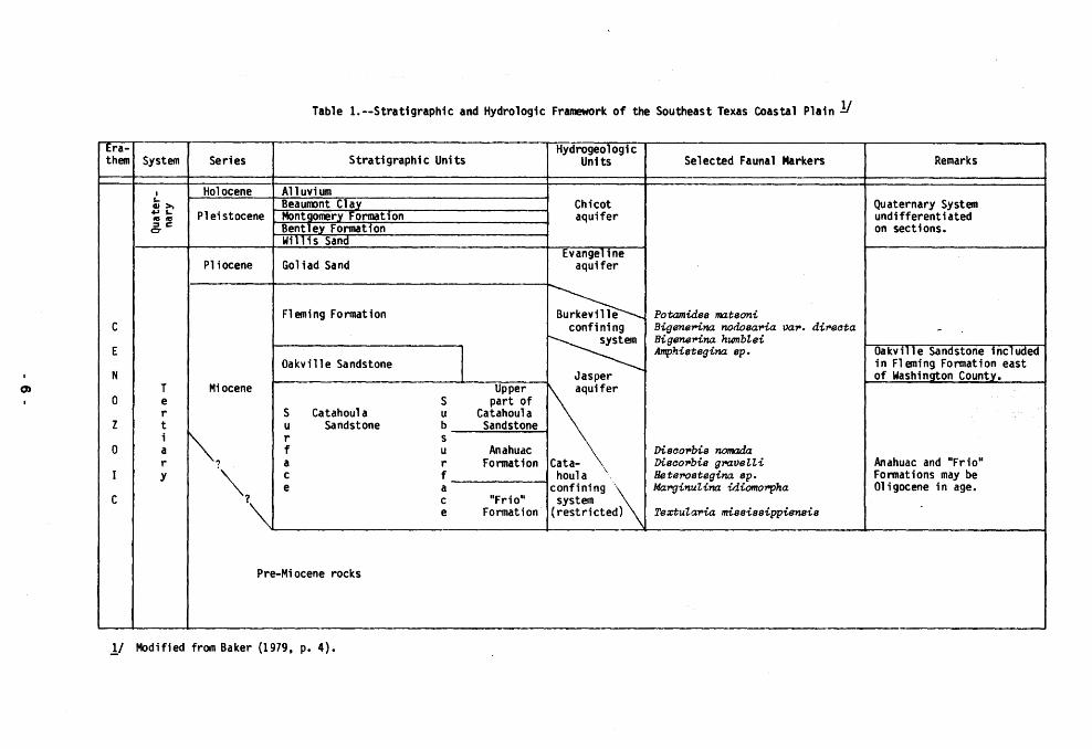
1. Stfatigraphic and Hydrologic Framework of the Southeast TexasCoastal Plain . . . . . . . .. . . . . . .. . . . . . . . . . . . . .. . . .. . . . . . . .. . . . . . . . . .. . ... . .. .. .. ... . .. .. .. . 6

FIGURES

1. Map Showing Location and Extent of the Study Area 2

2. Map Showing Location of Stratigraphic and Hydrologic Sections 5

3. Stratigraphic and Hydrologic Section A-A'

4. Stratigraphic and Hydrologic Section B-B'

5. Stratigraphic and Hydrologic Section C-C'

6. Stratigraphic and Hydrologic Section 0-0'

7. Stratigraphic and Hydrologic Section E-E'

7

9

11

13

15

8. Map Showing Altitude of the Top of the Jasper Aquifer 21

9. Map Showing Sites Where Moderate to Large Volumes of WaterAre Pumped From the Jasper Aguifer 25

viii

TABLE OF CONTENTS-Continued .

Page

10. HydrOgraphs of Water Levels in Selected Wells Completedin the Jasper Aquifer 27

11 . Map Showing Approximate Potentiometric Surface of theJasper Aquifer Prior to Development by Wells . . . . . . . . . . . . . . . . . . . . . . . . . . . . . .. . . . . . . . . 31

12. Diagram Illustrating Conceptual Model of the Ground-Water Hydrologyof the Texas Coastal Plain Prior to Development By Wells 33

Maps Showing:

13. Boundaries and Grid Patterns of the Model 35

14. Approximate Transmissivity in the Part of the JasperAquifer Containing Fresh to Slightly Saline Water 37

15. Distribution of Net Recharge as Equivalent Precipitationon the Outcrop of the Jasper Aquifer 41

16. Vertical-Hydraulic Conductivity of the BurkevilleConfining System 45

17. Thickness of the Burkeville Confining System 47

18. Approximate Potentiometric Surface of the EvangelineAquifer Prior to Development by Wells 51

19. Simulated Potentiometric Surface of the Jasper AquiferPrior to Development by Wells 53

20. Location and Node Designation of a Cross Section of theModel Used for Sensitivity Analysis 55

Profiles Showing:

21. Hydrologic Parameters and Hydraulic Heads of the Calibrated Modelfor the Cross Section Used for Sensitivity Analysis 57

22. Sensitivity of Calibrated Model to Variations in Transmissivityof the Jasper Aquifer 58

23. Sensitivity of Calibrated Model to Variations in Vertical-HydraulicConductivity of the Burkeville Confining System . . . . . . . . . . . . . . . . . . . . . . . . . . . . . . . . . . . . . 58

ix

TABLE OF CONTENTS-Continued

Ptag.

24. D,istribution of Leakage and Sensitivity of Water Levels to Reductionsin Recharge and Vertical-Hydraulic Conductivity on and Near theOutcrop of the Jasper Aquifer and Burkeville Confining System 60

26. Hydrologic Parameters for the Cross Section of the Model Extended into thePart of the Aquifer Containing SaltWater and Sensitivity of the CalibratedModel to the Downdip Extension . . . . . . . . . . . . . . . . . . . . . . . . . . . . . . . . . . . . . . . . . . . . . . . . . . . . . . 60

x

HYDROLOGY OF THE JASPER AQUIFER

IN THE SOUTHEAST TEXAS COASTAL PLAIN

E.T. Baker, Jr.U.S. Geological Survey

This report has been prepared to document the construction and calibration of a digital-computer model that simulates water flow in the Jasper aquifer of Miocene age in southeastTexas, and to present an account of the improvement in our understanding of the hydrology ofinterconnected aquifers and confining layers. It is in this area of Texas that the Jasper has itsgreatest ground-water potential. For this reason, only this segment of the aquifer, which extendsstatewide across the coastal plain of the State, has been modeled. The ground-water flow modelof the Jasper is designed to quantify certain hydraulic properties of the hydrologic system such asvertical-hydraulic conductivity and to a lesser extent, recharge and transmissivity, and to be usedas a tool to aid water planners in the regional development of the Jasper aquifer and in theprotection of its water supplies.

This report on the model also serves to improve our understanding of the hydrology of theinterrelationship of adjoining aquifer systems and confining systems. The improvement isachieved by the development of the digital model of the hydrologic system prior to significantground-water development.

The scope of this report directed primarily to a discussion of: (1) the geohydrology of theground-water system including the frame work of the southeastern Coastal Plain; (2) a discussionof the hydrologic and hydraulic parameters that are built into the model; and (3) a discussion ofthe calibration and various sensitivity analyses of the model including a steady-state simulationprior to development of the aquifer by wells.

This report constitutes the ultimate objective of a project to evaluate the ground-waterresources of the Miocene aquifer(s) in the Gulf Coastal Region of Texas. As an interim part of theproject, a report (Baker, 1979) was prepared to illustrate the stratigraphic and hydrogeologicframework of the Jasper aquifer as well as other hydrogeologic units from the Sabine River to theRio Grande (Louisiana to Mexico). This was shown by a series of 11 dip sections that are about 50miles apart and 100 miles long and 1 strike section 500 miles long. Ground water havingconcentrations of less than 3,000 mg/l (milligrams per liter) of dissolved solids (fresh to slightlysaline water) is shown on the sections and serves as an index to the availability of freshwater.

Description of the Study Area

The study area, which extends slightly beyond the modeled area, is about 25,000 squaremiles and is predominantly within the southeast Texas Coastal Plain (Figure 1). The eastern limitof the area, however, extends into western Louisiana from 20t050 miles. The western boundaryof the area is slightly west of the Brazos River and is about 170 miles west of the Texas-Louisianaborder. The northern boundary is the most inland extent of the Miocene-age formations(Catahoula Sandstone), which is about 100 miles inland from the coastline. The southernboundary of the described area approximates the coastline, although the model's southernboundary is from 30 to 50 miles inland from the Gulf of Mexico.

The land surface is mostly a smooth depositional plain in the southern two-thirds of the areaand a slightly rolling dissected terrain in the northern one-third. Altitudes range from sea level tomore than 600 feet in places on the outcrop of the Jasper aquifer.

Precipitation ranges from 40 to almost 60 inches, becoming progressively greater from westto east. The southeast Texas Coastal Plain is the area of greatest precipitation in the State, and forthis reason, the water tables of the aquifers are near the land surface.

oI

NEW MEXICO

50 100 150 200 MILESI I

OKLAHOMA

Figure 1.-Location and Extent of the Study Area

- 2 -

Several major streams cross the area in a southward direction and flow into the Gulf ofMexico. These include, from east to west, the Sabine, Neches, Trinity, San Jacinto, Brazos, andColorado Rivers. About 55 percent of the average annual runoff in Texas is transported by theserivers, their base flows being sustained by large volumes of seepage from the aquifers.

The economic development of the study area varies widely. The urbanized sections in thesouth part of the area have a large and diversified industrial base. Houston, the Beaumont-PortArthur-Orange complex, and Lake Charles are densely populated centers to the south with largepetrochemical industries. Extensive rice irrigation also is practiced in the south. The northernsections are largely rural with only a relatively small scattering of industry and less irrigatedfarming. Large volumes of surface and ground water are used by industry for cooling andprocessing purposes and by rice and cotton growers for irrigation. The rapid growth anddevelopment of much of the area is due to the accessibility and abundance of surface and groundwater. Not withstanding the fact that large volumes of water are pumped from various aquifersunderlying the Coastal Plain, the Jasper aquifer remains relatively undeveloped. This is primarilybecause it lies beneath two prolific aquifers -the Chicot and Evangeline-that because of theirshallower positions, are the more extensively pumped aquifers in the southern part of the area.

History of Hydrologic Modeling in the Texas Coastal Plain

The first attempt at modeling the ground-water system in the Texas Coastal Plain resulted inthe construction of an electrical-analog model of the Chicot and Evangeline aquifers in theHouston district (Wood and Gabrysch, 1965). This model covered an area of 5,000 square miles inall or parts of Harris, Galveston, Brazoria, Fort Bend, Austin, Waller, Montgomery, Liberty, andChambers Counties. It was used to predict water-level responses under various conditions ofpumping, but had only limited success because the Chicot and Evangeline were simulatedindependently, and agricultural pumping in the western part of the area could not be represented.The model indicated a need for improvement in aquifer delineation and a more adequate modelingof the aquifers’ transmissivities and the vertical leakage between them.

Ten years later, a second electrical-analog model was constructed incorporating additionalhydrologic data and more advanced concepts of the hydrologic system (Jorgensen, 1975). Thismodel, also of the Chicot and Evangeline aquifers, was larger than the first one and included anarea of about 9,000 square miles, with the Houston district as its center. The larger areaminimized the boundary effects within the Houston district, which were a problem with the firstmodel. The effects of the withdrawals of water from well fields for a year or longer were simulatedby this second electrical-analog model.

A third model, also of the Chicot and Evangeline aquifers and centering on the Houstondistrict, was constructed several years later (Meyer and Carr, 1979). The five-layer, finite-difference model used a digital computer for simulation of three-dimensional ground-water flowin an area of 27,000 square miles. This model simulated water-level responses to pumping,changes in storage in the clay layers, and land-surface subsidence.

The most recent hydrologic modeling of ground-water flow in the Chicot and Evangelineaquifers refined much of the previous work and extended coverage of these aquifers throughoutthe Coastal Plain of Texas (Carr and others, 1985). This work resulted in a series of multilayered,

-3-

three-dimensional models that alsosimulate the response of water levels to pumping, changes in .storage in the clay layers, and land-surface subsidence.

Metric Conversions

For those readers interested in using the metric system, the metric equivalents of inch­pound units of measurements are given in parentheses. The inch-pound units used in this reporthave bee" converted to metric units by the following factors:

From

feet

feet per day (ftld)

feet per mile (ft/mi)

feet per second (ft/s)

squar~ feet per day(ft2/d)

gallons per minute(g~l/min)

inches

miles

milli~n gallons perday (Mgalld)

square miles

Multiply by

0~3048

0.3048

0.189

0.3048

0.0929

0.06309

25.4

1.609

0.04381

2.590

To obtain

meters (m)

meters per day (mid)

meters Per kilometer (m/km)

meters per second (m/s)

square meters per day(m2/d)

liters per second(lIs)

millimeters (mm)

kilometers (km)

cubic meters persecond (m3/s)

square kilometers (km2)

National Geodetic VerticalDatum of 1929 (NGVD of 1929): A geodetic datum derived from ageneral a~justment of the first-order level nets of both the United States and Canada, formerly

I called mean sea level. NGVD of 1929 is referred to as sea level in the text of this report.

GEOHYDROLOGIC FRAMEWORK OF THESOUTHEAST TEXAS COASTAL PLAIN

Miocene and younger sediments that underlie the southeast Texas Coastal Plain and thatform impprtant hydrologic units are thousands of feet thick at the coastline. These clasticsediments constitute geologic formations, which collectively or in part, form important hydrologic

- 4 -

units. The geologic formations and··tiydrologic units are composed of varying proportions ofgravel, sand, silt, and clay. They thicken toward the Gulf of Mexico and are inclined in thatdirection. The younger geologic formations and hydrologic units crop out nearer the Gulf and theolder ones farther inland. All of them have outcrops or subcrops that are virtually parallel to theshoreline.

In the following discussion, e~phasis is placed on the geologic and hydrologic units ofMiocene age. It is necessary, however, to discuss the older and younger units in order tounderstand their relationship, both stratigraphically and hydrologically, to the Miocene.(Stratigraphic and geologic units that are pertinent to the discussion are described in Table 1.Theunits were determined from several sources and may not necessarily follow the usage of the U.S.Geological Survey.) Four dip sections and one strike section are located in Figure 2 and arepresented in Figures 3-7 to visualize the interrelationships and to show the presence of waterhaving concentrations of less than about 3,000 mg/I of dissolved solids within the units.

EXPLANATION

~ OUTCROP OF JASPER AQUIFER

ot

Pre-~iocene

50 MILESI

Figure 2.-Locationof Stratigraphic and Hydrologic Sections

Stratigraphic Units

Pre-Miocene rocks are composed of beds of sand, clay, carbonate rocks, and other rock typesthat are tens of thousands of feet thick. Within this thick section of rocks that underlie the Jasper

- 5 -

0)

Table l.--Stratigraphic and Hydrologic Framework of the Southeast Texas Coastal Plain !I

Era- Hydrogeologicthem System series Stratigraphic Units Units Selected Faunal Markers Remarks

• Holocene Alluvium'- BeaulOOnt Clay Chicot Quaternary SystemQI>'~'- Pleistocene MontQOmerv Formatlon aquifer undifferentiatedlUlU;:,c Bentley Formation on sections.0'

Will is SandEvangeline

Pliocene Gol iad Sand aquifer

Fleming Formation ~ Potamides matsoniC confining BigeneJOina nodosa'l"ia va.,.. di1'eota -

~BigeneJOina hwnb1.ei

E

IAmphistegina sp. Oakville Sandstone included

Oakville Sandstone in Fl eming Formation eastN Jasper of Washington County.

T Miocene Upperi\fer0 e S part of

r S Catahoula u CatahoulaZ t u Sandstone b Sandstone

i

""1r s

0 a f u Anahuac Disoo.,.bis namadar a r Formation Cata- \ Disoo.,.bis grtave1.1.i Anahuac and "Frio·'

I y

"'1c f houla· Hete1'ostegina sp. Formations may bee a confining :'\ Ma1"!1if1u1.ina idiomo1'pha Oligocene in age.

C c "Frio·' system.~ e Formation {restricted) Textu1.a.,.ia mississippiensis

Pre-Miocene rocks

1/ Modified from Baker (1979. p. 4).

aquifer are identifiable stratigraphic units. These units are not delineated on the sectionsincluded with this report; however, a discussion of these units and their identity in the subsurfaceto a depth of about 8,000 feet are presented by Baker (1979).

The stratigraphic units of pre-Miocene age are hydrologically significant. Some are aquifersand others are confining layers. The hydrologic relationship of the Jasper aquifer to theunderlying contiguous units is of primary importance from the standpoint of boundary effects onthe digital model. Stratigraphic examination of geophysical logs indicates, however, thatfreshwater in the stratigraphic units of pre-Miocene age is separated from water in the Jasper byconfining layers.

Miocene

The outcropping stratigraphic units that are designated as Miocene in age are, from oldest toyoungest, the Catahoula Sandstone, Oakville Sandstone, and Fleming Formation. The “Frio”Formation, Anahuac Formation, and a unit, that is referred to in this report as the upper part of theCatahoula Sandstone, are assigned by the author as possible downdip equivalents of the surfaceCatahoula although the Anahuac and “Frio” Formations may be Oligocene in age. The data inTable 1 and the dip sections (Figures 3-6) illustrate this relationship.

The Catahoula Sandstone is a pyroclastic unit that has been independently mapped on theoutcrop by various geologists with little modification. Within the report area, it is composed of

interbedded and interlensing sand and clay. The dip sections show that the thickness of theCatahoula increases downdip at a large rate. It eventually includes, when the AnahuacFormation is reached at depths of about 2,800 to 3,600 feet below sea level, the “Frio” Formation,the Anahuac Formation, and the upper Catahoula unit.

The Oakville Sandstone and Fleming Formation are composed almost entirely of terrigenousclastic sediments that form sand and clay interbeds. Their boundaries are discernible contacts in

some areas and arbitrary ones within zones of lithologic gradation in other areas.

Within the limits of the report area, the Oakville Sandstone on the surface is recognized andmapped as a formation only west of the Brazos River in Washington County. Here itspredominantly sandy character is barely distinguished from the overlying Fleming Formation,which is only slightly less sandy. Eastward from the vicinity of the Brazos River, the Oakvillegrades into the base of the Fleming. The position of the base of the Oakville in the deeper parts ofthe subsurface has been delineated on section D-D’ (Figure 6) merely as an approximation.

The Fleming Formation, which is the uppermost unit of Miocene age, is lithologically similarto the Oakville Sandstone. Where the Fleming is not separated from the Oakville and directlyoverlies the Catahoula Sandstone from about Grimes County to the Sabine River, the percentageof sand in the formation increases eastward. In the far eastern part of the study area, the quantityof sand in the formation greatly exceeds the quantity of clay. This can be seen in strike sectionE-E’ (Figure 7). .

Post-Miocene

The stratigraphic units of post-Miocene age consist chiefly of interbedded sand and clay andsubordinate beds of silt and gravel. Collectively, they are estimated to be in excess of 2,000 feet

- 17 --

thick at the coastline in southeast Texas. This wedge of clastic sediment rapidly thins inland fromthe coastline to extinction along an irregular line from 70 to 100 miles inland from the coastline.

The Goliad Sand of Pliocene age; Willis Sand, Bentley Formation, Montgomery Formation,and Beaumont Clay of Pleistocene age; and alluvium of Holocene age comprise the post-Miocenesediments. All of these units are similar in lithology, and for this reason, delineation usingelectrical logs has not been attempted on the stratigraphic and hydrologic sections.Notwithstanding, the difficulty in identifying these stratigraphic units individually in thesubsurface, as a group they constitute significant aquifers in the southeast Texas Coastal Plain.

Hydrologic Units

The fallowing discussion will emphasize five hydrologic units-the Catahoula confiningsystem (restricted), which underlies the Jasper aquifer; the Jasper aquifer; and the Burkevilleconfining system and the Evangeline and Chicot aquifers, which overlie the Jasper. Thehydrology of the units underlying and overlying the Jasper is important for understanding thewater flow system in the Jasper and for modeling the aquifer.

Catahoula Confining System (Restricted)

The Catahoula confining system (restricted), which was named by Baker (1979) after theCatahoula Sandstone, is treated in this report as a quasi-hydrologic unit. In most of southeastTexas, this confining system has different boundaries than the stratigraphic Catahoula. Its top(base of the Jasper aquifer) is delineated along lithologic boundaries that are time-stratigraphicin some places, but transgress time lines in other places. Its base, which coincides with the baseof the stratigraphic unit, is delineated everywhere in the report area along time-stratigaphicboundaries that are independent of lithology. No attempt was made to establish a lithologic(hydrologic) base for the unit, which would have created a distinct hydrologic unit. Such an effectwould have involved a thorough hydrologic evaluation of pre-Miocene formations, which wasbeyond the scope of this study.

In some places, the Catahoula confining system (restricted) is identical to the stratigraphicunit, but there are notable exceptions. These departures of the hydrologic boundaries from thestratigraphic boundaries are most prominent in the eastern part of the study area near the SabineRiver (Figure 7) and in numerous places at the outcrop and in the shallow subsurface (Figures3-6). In these places, the very sandy parts of the Catahoula Sandstone (stratigraphic unit) that lieimmediately below the Oakville Sandstone or Fleming Formation are included in the overlyingJasper aquifer. This leaves a lower section from 0 to 2,000 feet or more in thickness that consistspredominantly of clay or tuff with some interbedded sand to compose the Catahoula confiningsystem (restricted). In most places, this delineation creates a unit that generally is deficient insand so as to preclude its classification in these areas as an aquifer. For this reason, in most of itsshallow to moderately deep subsurface extent, the Catahoula confining system (restricted)functions hydrologically as a confining layer that greatly restricts interchange of water betweenthe overlying Jasper aquifer and the underlying aquifers.

The quantity of clay and other fine-grained clastic material in the Catahoula confiningsystem (restricted) generally increases downdip, until the Anahuac Formation is encountered at

- 18 -

depths of 2,800 to 3,600 feet below sea level. Below this level, the “Frio” Formation becomescharacteristically sandy and contains moderately saline water to brine (3,000 to more than35,000 mg/l of dissolved solids) that extends to depths of many thousands of feet.

Jasper Aquifer

The Jasper aquifer, which was named by Wesselman (1967) for the town of Jasper in JasperCounty, Texas, until recently had not been delineated farther west than Washington, Austin, andFort Bend Counties in southeast Texas. Recently, delineations of the Jasper, as well as otherrelated hydrogeologic units, were made by Baker (1979) across the Coastal Plain of Texas fromthe Sabine River to the Rio Grande.

The configuration of the Jasper aquifer in the subsurface, as shown in the sections, isgeometrically irregular because the delineation was made on the basis of the aquifer being arock-stratigraphic unit. The hydrologic boundaries were defined from observable physical(lithologic) features rather than from inferred geologic time lines, which do not necessarilycorrespond to Iithologic features.

The position of the base and top of the Jasper aquifer in southeast Texas transgressesstratigraphic boundaries along strike and downdip. The base of the aquifer coincides with thestratigraphic lower boundary of the Oakville Sandstone or Fleming Formation in some places. Inother places, the base of the Jasper lies within the Catahoula Sandstone or coincides with thebase of that unit. The top of the aquifer is within the Fleming in places and is within the Oakville inother places. The dip of the top of the Jasper is fairly uniform in rate within the zone of fresh toslightly saline water. Within this zone, which is about 50 to 75 miles in width, the dip averagesabout 55 ft/mi to the south-southeast (Figure 8).

The Jasper aquifer ranges in thickness, where it is not eroded, from as little as 200 feet toabout 3,200 feet within the area of its delineation. The maximum thickness occurs in the regionwhere the aquifer contains moderately saline water to brine. An average range in thickness of theaquifer within the zone of water having concentrations of less than 3,000 mg/l of dissolved solidsis from about 1,000 to 1,500 feet. At the Sabine River, the Jasper attains a thicknessof 2,400 feetin well 12 in section E-E’ (Figure 7), where the aquifer is composed predominantly of sand. Thispredominance of sand in the Jasper in the eastern part of the study area, however, diminishes ina westward direction.

The Jasper aquifer contains water having concentrations of less than 3,000 mg/l ofdissolved solids from its outcrop to about 50 to 75 miles downdip from its outcrop. This downdiplimit approximately parallels the coastline passing a few miles north of Beaumont and near thecenter of Houston. Water having concentrations of less than 3,000 mg/l of dissolved solidsoccurs in the Jasper as deep as 3,000 feet below sea level in section D-D’ (Figure 6). Althoughpumpage from the Jasper is not significant, it is capable of yielding 3,000 gal/min or more ofwater to wells in certain areas.

Burkeville Confining System

The Burkeville confining system was named by Wesselman (1967) for outcrops near thetown of Burkeville in Newton County, Texas. It separates the Jasper and Evangeline aquifers andretards the interchange of water between the two aquifers.

-19-

The Burkeville confining system is a rock-stratigraphic unit predominantly consisting of siltand clay. Upper and lower boundaries of the unit do not strictly correspond to geologic timeboundaries, although in some places the unit appears to possess approximately isochronousboundaries. The configuration of the top and bottom of the unit is irregular. Boundaries are notrestricted to a single stratigraphic unit, but are included within the Fleming Formation andOakville Sandstone in some places. This is shown in section D-D’ (Figure 6).

The thickness of the Burkeville confining system ranges from about 100 to 1,000 feet. Ingeneral, the greatest variations occur in the relatively deep subsurface within the zone ofmoderately saline water to brine. A typical thickness of the Burkeville is about 300 feet.

The Burkeville confining system is predominantly composed of fine-grsined materials, suchas silt and clay, as shown in numerous geophysical logs. In most places, these fine-grainedsediments are interbedded with sand lenses, which contain fresh to slightly saline water. Someof these sand lenses yield water to small-capacity wells. Because of its relatively largepercentage of silt and clay when compared to the underlying Jasper aquifer and overlyingEvangeline aquifer, the Burkeville is a confining unit. The effectivenessof the unit as a confininglayer is further borne out by the fact that hydro-static pressures in the Jasper and Evangeline arenotably different immediately above and below the Burkeville where detailed testing by welldrillers has been done.

Evangeline and Chicot Aquifers

The Evangeline and Chicot aquifers were named and defined by Jones (Jones, Turcan, andSkibitzke, 1954) for ground-water reservoirs in southwestern Louisiana. They also have beenmapped in Texas, but until recently, had not been delineated farther west than Washington,Austin, and Fort Bend Counties in southeast Texas. Their positions in the Coastal Plain of Texaswestward to the Rio Grande are now known from mapping by D. G. Jorgensen, W. R. Meyer, andW. H. Sandeen of the U.S. Geological Survey (Baker, 1979).

The Evangeline aquifer primarily has been delineated as a rock-stratigraphic unit. Althoughthe aquifer is composed of at least Pliocene-age sediments, its lower boundary crosses time linesto include sections of sand in the Fleming Formation. Within most of the study area, theEvangeline at the surface includes about the upper one-third of the Fleming outcrop as seen insections A-A’, B-B’, and C-C’ (Figures 3-5). In the western part of the area where the OakvilleSandstone is recognized, the Evangeline includes more than three-fourths of the Flemingoutcrop as seen in section D-D’ (Figure 6). The upper boundary of the aquifer probably closelyfollows the top of the Pliocene-age sediments or the Goliad Sand, which is not exposed, exceptperhaps in a few isolated places, in the report area. This stratigraphic relationship of the top of theEvangeline is somewhat speculative.

The Chicot aquifer has been defined to exclusively include the Quaternary age sediments. Itsdelineation in the subsurface on this stratigraphic basis is problematical due to the difficulty inidentifying the base of the Quaternary deposits on electrical logs. This subsurface delineation insoutheast Texas has been based largely on the presence of a greater sand-to-clay ratio in theChicot than in the underlying Evangeline aquifer. In some places, a prominent clay layer has beenused as the boundary. Differences in hydraulic conductivity or water levels in some areas also

- 23 -

have been used to differentiate the Chicot from the Evangeline. At the surface, the base of theChicot on the sections has been picked at the most landward edge of the oldest, undissectedcoastwise terrace of Quaternary age.

The Evangeline and Chicot aquifers are typically wedge-shaped and have a large sand-to-clay ratio. Individual sand beds are characteristically tens of feet thick. Near the outcrop, theEvangeline ranges in thickness from about 400 to 600 feet but near the coastline, where theaquifer’s top is about 1,200 feet deep, its thickness averages about 2,300 feet. Water havingconcentrations of less than 3,009 mg/l of dissolved solids is not present in the aquifer, at thecoastline. The Chicot attains a thickness of about 1,200 feet at the coastline, where, in places, itstill contains water having concentrations of less than 3,000 mg/l of dissolved solids in most ofits full thickness (Figures 5 and 6).

Huge quantities of water are pumped from the Chicot and Evangeline aquifers for municipalsupply, industrial use, and irrigation. The most extensive and concentrated development is in theHouston area, where large-capacity wells yield from 1,000 to more than 3,000 gal/min andaverage about 2,000 gal/min.

GROUND-WATER DEVELOPMENT

The Jasper aquifer regionally is relatively undeveloped. This primarily is because it underliesthe Evangeline and Chicot aquifers, which are capable of supplying large volumes of adequate-quality water for most needs. Most of the wells that produce water from the Jasper are located onits outcrop and short distances downdip where the Burkeville confining system is exposed, orwhere the Chicot and Evangeline are not thick enough to provide sufficient water to largecapacity wells.

Moderate to large volumes of water are pumped locally from the Jasper aquifer only in a fewwidely spaced localities (Figure 9). These centers of pumpage are mostly towns and industrialsites, where one or more public-supply or industrial wells are usually within the confines of thecity limits or at individual industrial sites. By far, the largest withdrawal of water within themodeled area is in Beauregard Parish near De Ridder, Louisiana, where industrial usageexceeded 20 Mgal/d during 1979. This site is about 10 miles east of the Sabine River. Elsewhere(Figure 9), municipal or industrial pumpage at any one site is many orders of magnitude smallerthan the pumpage near De Ridder and ranges from 0.10 to 4.0 Mgal/d.

As a result of the relatively limited development in the Jasper aquifer in southeast Texas,water levels have remained near the land surface, and only slight water-level declines haveoccurred regionally. Water-level trends in the Jasper aquifer for several representative wells areshown in Figure 10. Some of these wells are in pumping centers, whereas others are away fromsuch centers. The hydrographs show that there have been, for the most part, only slight declinesof 10-l5 feet in 20 years in the potentiometric surface at those sites.

The potentiometric surface of the Jasper aquifer prior to well development has beenapproximated on the basis of the earliest available water levels. To approximate predevelopmentconditions, the hydraulic heads have been adjusted upward in varying amounts by backwardprojection of hydrographs and, in some areas, by considering heads measured in nearby wells

- 24 -

that represented pressures little affected by pumping stresses. The potentiometric contoursreflect these adjustments, while the well data indicate actual measured water levels prior to anyadjustment (Figure 11).

DESCRIPTION OF THE DIGITAL MODEL

The digital model that was developed to simulate the ground-water hydrology of the Jasperaquifer is a mathematical, two-dimensional, finite-difference program that was documented byTrescott, Pinder, and Larson (1976). The iterative-numerical technique used to solve thesimultaneous equations is the strongly implicit procedure (SIP). This procedure was originallydescribed by Stone (1968) for problems in two dimensions.

The steady-state approach was used to simulate the hydrologic conditions in the aquifer.This approach was taken because, on a regional basis, the aquifer is only slightly stressed frompumping, and in many places, groundwater levels are virtually static, which indicates a nearlysteady-state condition. For this reason, no attempt was made to develop a transient model tosimulate the small regional water-level changes that have occurred since pumping began. Thesteady-state model developed for the project area, therefore, represents hydrologic conditionsprior to development by wells, when natural recharge equaled natural discharge and water levelsvaried little during long periods.

The Jasper aquifer is part of an extensive and continuous hydrologic system in the GulfCoastal Plain; its lateral boundaries are far beyond the modeled area. The aquifer containsfreshwater for varying distances downdip beyond which the aquifer contains saltwater. Formodeling purposes, however, only the part of the aquifer containing fresh to slightly saline waterwas considered. Under steady-state conditions, the interface between the fresh to slightly salinewater and saltwater is assumed to be static and is considered to be a no-flow boundary. Beyondthe interface on the downdip side, the saltwater is virtually motionless, whereas on the updipside, the fresh to slightly saline water is circulating throughout the aquifer. From the outcrop,water as recharge (a finite flux or constant recharge boundary in the model) moves downdipbeneath the Burkeville confining system. Here two components of movement are in effect. One isa downdip component, and the other is an upward component. Where the Jasper is overlain bythe Burkeville, water is being discharged through the Burkeville as steady leakage, with the sumof the leakage equal to the sum of the net recharge. The contact of the base of the Jasper with theunderlying Catahoula confining system (restricted) is treated as a no-flow or zero-flux boundary,as the Catahoula functions in the hydrologic system as a confining layer of mostlyclayor tuff thatfor all practical purposes prevents any significant interchange of water between the Jasper andunderlying aquifers. (See Figure 12.)

The model has a grid pattern of 15 x 24 nodes representing an area of about 20,000 squaremiles as shown in Figure 13. In the outcrop of the Jasper aquifer, the grids have dimensions of5 x 10 miles and are the smallest in the model. The purpose of using the smaller grids is to providea better distribution of net recharge on the relatively narrow outcrop of the aquifer. Downdip fromthe outcrop, where the aquifer is beneath the Burkeville confining system, the model has griddimensions of 10 x 10 miles. Within any one grid, the aquifer properties are assumed to beuniform.

- 29 --

Constant- recharoe I

: boundary (constan7fIUX) :I II I Direction of oround-water

~~:=~=~~S::§:;:;~i::=====:;:::==~b~m~ove~me~n~t~;;::::::.--.......JSea ~ Sealevel level

Not to scale

Figure 12.-Conceptual Model of the Ground-Water Hydrology of the Texas CoastalPlain Prior to Development by Wells

Impermeable (no-flow) boundaries were placed at the two lateral extremities of the modelsufficiently far beyond the main study area to decrease any boundary effects in the area ofinterest. At the downdip edge of the model, a no-flow boundary also was placed sufficiently farenough into the part of the aquifer containing saltwater so that the boundary would havenegligible effect on the part of the aquifer containing fresh to slightly saline water. The updip edgeof the outcrop was a natural physical boundary having zero flow.

The boundary effects in the model were tested by substituting constant-head boundaries forthe no-flow boundaries at the two lateral extremities on the east and west and on the downdipextremity on the south. Hydraulic heads representing the approximate potentiometric surface ofthe Jasper aquifer prior to development by wells (Figure 11)constituted the starting-head matrix.The results showed very little difference (less than 2 feet) even within 10 miles of the adjacentconstant-head boundaries. Most nodes showed no differences, and where differences did occur,they were rises of no more than 1 foot.

Aquifer Properties and Parameters Modeled

Transmissivity of the Aquifer

All known aquifer tests conducted in wells completed in the Jasper aquifer within themod.led area were examined. From these tests, horizontal hydraulic conductivities werecomputed, and horizontal hydraulic-conductivity maps and sand-thickness maps were prepared.The areal distribution of transmissivity of the Jasper was then determined (Figure 14).

- 33 -

The transmissivity of the Jasper aquifer ranges from less than 2,500 ft2/d in places in theoutcrop and near the downdip limit of fresh to slightly saline water to about 35,000 ft2/d east ofthe Sabine River. Outcrop transmissivities increase eastward as do transmissivities in theartesian part beneath the Burkeville confining system. These increases are attributed primarily toeastward increases in sand thicknesses. Conversely, the decreases in transmissivities near thedowndip limit of fresh to slightly saline water are due to the fact that the thickness of sand withthis quality water decreases to zero at this southern interface.

Recharge to the Aquifer

Precipitation on the outcrop of the Jasper aquifer is the source of recharge to the aquifer.Only a small part of the total precipitation, however, does not run off directly or is notevapotranspired, and a large part of the precipitation that reaches the zone of saturation in theoutcrop moves to streams where it is discharged as seepage and springflow. Therefore, only asmall quantity of water from precipitation becomes net recharge, or that quantity of water thatmoves into the downdip part of the aquifer south of the outcrop. Under steady-state conditions inthe Jasper as conceptualized prior to development by wells, this net quantity of recharge is equalto the quantity of discharge by vertical leakage through the Burkeville confining system.

In the model, the outcrop was treated as a constant-recharge (constant-flux) boundary witheach node constantly recharging a given volume of water. The total net recharge was determinedincrementally for each 10-mile length of the Jasper aquifer's outcrop using the Darcy flowequation in the following form:

a =TIL,

where a =flow rate, in cubic feet per day;

T = transmissivity, in square feet per day;

I = hydraulic gradient, in feet per mile; and

L = length of aquifer (in miles) across which the flow moves.

(1 )

The 1O-mile cross-sectional length of the outcrop, which the flow moves across, was chosen atthe outcrop's contact with the overlying Burkeville confining system. The flow thus determined tobe moving into the downdip artesian parts of the aquifer can be equated with the total netrecharge for the incremental area of the outcrop. This volume of recharge was then apportionedto the nodes within that part of the outcrop. The distribution of total net recharge as equivalentprecipitation on the outcrop of the Jasper is shown in Figure 15.

The quantity of water as net recharge to the Jasper aquifer is equivalent to 0.9 inch ofprecipitation on the sandy part of the outcrop, about 2 percent of the average precipitation. Inaddition to this quantity, according to Wood (1956, p. 30-33), about 1 inch or more of precipitationenters the outcrop but is discharged to streams crossing the outcrop as base flow or rejectedrecharge.

- 39 -

Leakage Through the Burkeville Confining System

Water in the Jasper aquifer downdip from the outcrop is discharged upward through theBurkeville confining system. This process is simulated in the model by considering the vertical-hydraulic conductivity of the Burkeville, the thickness of the Burkeville, and the hydraulic head onthe upper side of the Burkeville which is the predevelopment potentiometric surface of water inthe Evangeline aquifer.

Vertical-Hydraulic Conductivity of the Burkeville Confining System

The effective vertical-hydraulic conductivity of the Burkeville confining system is a functionof the composite intergranular flow characteristics of the predominantly silt and clay beds thatcompose this hydrologic unit. Hydraulic-conductivity values, which were determined bycalibration of the model, range from 1.0 x 10-5 to 2.5 x 10-3 ft/d. These values are similar tothose determined for the clay beds in the Chicot and Evangeline aquifers by previous modelstudies in the Houston area and in other areas along the Gulf Coast of Texas (Jorgensen, 1975, p.54; Meyer and Carr, 1979, p. 17; and Carr and others, 1985). In these areas, the vertical-hydraulicconductivity of the Chicot and Evangeline, which is controlled primarily by the clay beds thatoccur within the vertical sequence of sand beds, ranges from 9.2 x 10 -5 to 2.3x 10-4 ft/d.

The larger values of vertical-hydraulic conductivity of the Burkeville confining system areassociated with the outcrop and updip parts of the hydrologic unit, and the smaller values areassociated with the downdip parts. This pattern of differing vertical hydraulic conductivities isshown in Figure 16. Sedimentation features of the Burkeville support this pattern as increasinglyfiner grained sediments were deposited in the downdip direction (Baker, 1979, p. 40).

Thickness of the Burkeville Confining System

Large variations in the thickness of the Burkeville confining system affect the leakage at eachnode in the model where the confining system overlies the Jasper aquifer. All areas of the Jaspersouth of its outcrop are overlain by the Burkeville, and in no place are the Evangeline or Chicotaquifers, which overlie the Burkeville, in contact with the Jasper.

Large thicknesses of the Burkeville confining system of more than 600 feet are present inseveral grids near the southeastern boundary of the model, and even larger thicknesses of morethan 900 feet are present in a few grids along the western boundary near the downdip limit offresh to slightly saline water in the Jasper aquifer. In other places between these two areas-chiefly in the outcrop of the Burkeville where it thins to extinction-the thickness of the confiningsystem, is less than 100 feet as shown in Figure 17. Leakage is facilitated along the outcrop wherethe vertical-hydraulic conductivity generally is greater than elsewhere and where the confininglayers are relatively thin.

Head Differences Across the Burkeville Confining System

The flux across the Burkeville confining system in the model is controlled in part by thehydraulic head differences in the Evangeline and Jasper aquifers. In the steady-state model, the

- 43 - -

predevelopment potentiometric surfaces were approximated for the two aquifers using availablewater-level data, and the hydraulic head differences were determined. The approximatepredevelopment potentiometric surface of the Evangeline aquifer is shown in Figure 18. The mapis based on the oldest available water levels adjusted upward by varying amounts for some sitesto account for the effects of development. The predevelopment potentiometric surface of theJasper aquifer is shown in Figure 11.

Hydraulic-head differences between the Evangeline and Jasper aquifers varied significantlyprior to well development. As simulated in the model, these differences were less than 15 feet formost nodes near the updip reaches of the overlying Evangeline aquifer, and gradually increaseddowndip ranging from 70 to 130 feet at nodes along the southern limit of fresh to slightly salinewater in the Jasper. At all nodes, the predevelopment head in the Jasper was greater than thepredevelopment hydraulic head in the Evangeline. It should be noted that postdevelopmenthydraulic head changes in the Evangeline as well as in the Jasper could alter the magnitude ofthe hydraulic head differences across the Burkeville confining system or possibly even reversethe direction of water movement. These changes would have to be considered in any leakagedeterminations for a transient model.

Calibration of the Model

The model was calibrated by simulating the predevelopment hydrologic conditions of theJasper aquifer and comparing the computed potentiometric surface with the predevelopmentsurface that was based on historical water-level measurements. Where the computed surfacediffered significantly from the measured surface, vertical-hydraulic conductivity of the Burkevilleconfining system was modified, and the model was tested again. Transmissivity of the Jasperaquifer was modified in some areas, but to a much lesser extent than vertical-hydraulicconductivity of the Burkeville, because aquifer-test results were available for computingtransmissivity. This trial and error procedure was continued using reasonable modifications untila satisfactory match with the approximate potentiometric surface shown in Figure 11 wasobtained (Figure 19).

Results of the calibration show that the simulation basically agrees in most areas with thehistorical records of water levels. A good match was achieved in the artesian part of the aquifersouth of the outcrop. In the outcrop, the influence of semiartesian conditions in combination withrolling topography and associated variable transmissivity in short distances creates an irregularpotentiometric surface. For these reasons, simulations of the potentiometric surface are lessexact in the outcrop than elsewhere.

The water-level data in Figure 19 are the oldest available data that represent approximatepredevelopment conditions. Actual predevelopment water levels were greater in some areas, butthe data presented give a basis for comparison with the simulated water-level contours.

Sensitivity Analysis

Sensitivity of the model was demonstrated by hydrologic analysis primarily using a singlemodel column or cross section. This procedure simulated a one-dimensional flow tube along a

- 49 -

line of ground-water flow from the outcrop of the Jasper aquifer into the part of the aquifer thatcontains saltwater. The position of this cross section and arrangement of cells from node 2 on theoutcrQP to node 27, which is about 60 miles downdip from the limit of the fresh to slightly salinewater, are shown in Figure 20. The calibrated values of transmissivity of the Jasper aquifer, ofverticejll-hydraulic conductivity and thickness of the Burkeville confining system, and ofpotentiometric heads within the Jasper and Evangeline aquifers for appropriate nodes along thecross section are illustrated in Figure 21. Using these calibrated data and by varying the datavalues, as well as extending them beyond the model's downdip no-flow boundary at node 16,head values were simulated to show the changes in water levels that resulted from suchmodifications. Although the resulting changes in water levels pertain to the line of sectionrepresented by the flow tube, similar effects are expected to apply elsewhere in the model.

The changes in hydraulic head representthe result of new equilibriums being estab­lished in the aquifer from the uniformincreases and decreases in transmissivity. Auniform 25-percent increase in transmissivitycaused a decrease in the hydraulic gradient (aflattening of the potentiometric surface),

16146 8 10 12

NODE DESIGNATION OF CROSS SECTION

4o'----l---L--'---I---A----L---L---L..-~"""---'--.&....-...l~

2

Figure 21.-Hydrologic Paremeten and HydraulicH.ds of the Calibrated Model for the Cro..

Section Used for Sensitivity Analysis

The sensitivity analysis for transmissivity showed that a uniform 25-percent increase in thisparameter from that of the calibrated model resulted in a maximum decrease in head of 11 feet in

the updip limit of the aquifer's outcrop at node2 and a maximum increase in head of 10 feetat the downdip limit of water containing lessthan 3,000 mg/l of dissolved solids at node16. A uniform decrease of 25 percent in

,transmissivity resulted in a maximumincrease in head of 18 feet at the updip limit ofthe aquifer's outcrop to a maximum decreasein head of 13 feet at the downdip limit of 3,000mg/l water. If the calibrated values of trans­missivity that are uniformly decreasing fromnode 6 to 12 are extended as a straight-lineprojection to node 16, then this results in anincrease in transmissivity Qf as much as about7,500 ft2/d over the calibrated model, which,in turn, causes a maximum increase in head of4 feet. (See Figure 22.) The projected increasein transmissivity from nodes 12 to 16 negatesthe gradual decrease in transmissivity of thecalibrated model as the downdip limit of freshto slightly saline water, which serves as ano-flow boundary, is approached. This proce­dure compares the sensitivity of the no-flowboundary as an interface of fresh to slightlysaline water with more highly saline water.

- 57 -

16

r25-percent increase

-----------------

25-percent decrease~ --------

4 6 8 10 12 14

NODE DESIGNATION OF CROSS SECTION

20

10

vi'~ 0>-~a::w -10....<3

~

w -20<.!lz<::z:u

-30

-40

150

>-.... ~_0

~ro;t.... 0u ....;:)oxz~

0uozuO- U....I W;:) VI

~a::o w>- Q.::z: ....I....I W<w 10~u.

..... z~->-

02

164 6 8 10 12 14

NODE DESIGNATION OF CROSS SECTION

Straight-line projection of calibratedvalues from nodes 12 to 16-----,

\~."pe~:~~~~~:~~"lib"". mo'el~" ------",1 "

/

" ---- --- \/r //"'calibrated model '" "

/ ~~...25-percent decrease in cal ibrated model J '~

o

20

-20

Effect of 25-percent increase \

10 '"ffect of strai ght-l ine projection ""'\ __\.

\ ----,,----------------

," -- --~" ------" --..........~ -10'" --7-

~ £ffect of 25-percent decrease J -

25,000

20,000

~IX:UJ

15.000Il-....UJ

~UJIX: 10,000<t::>0l/l

~5,000

02

Figure 22.-Sensitivity of Calibrated Modelto Vari.tions in Transmissivity of

the Jasper Aquifer

Figure 23.-Sensitivity of Calibrated Model toVariations in Vertical-Hydraulic Conductivity

of the Burkeville Confining System

whereas a 25-percent decrease in transmissivity caused an increase in the hydraulic gradient (asteepening of the potentiometric surface). This is in accordance with the Darcy flow equation(equation 1) where the hydraulic gradient is inversely proportional to the transmissivity. Thedecrease in hydraulic head in the outcrop (with a uniform 25-percent increase in transmissivity)necessitates a rise in hydraulic head downdip, and conversely, with a 25-percent decrease intransmissivity, the increase in hydraulic head in the outcrop requires a decrease in hydraulic headdowndip-the flow rate or recharge being held constant.

A uniform 25-percent increase in the vertical-hydraulic conductivity of the Burkeville confin­ing system from that of the calibrated model resulted in a decrease in water levels from 3 feet inthe outcrop of the aquifer to 11 feet near the downdip limit of 3,000 mg/I water at node 16. Auniform 25-percent decrease in the vertical-hydraulic conductivity resulted in an increase inwater levels that ranged from 5 feet in the aquifer's outcrop to 15 feet at node 16. If thevertical-hydraulic conductivity remains constant throughout the model at 16.7 x 10- 10 ft/s, thewater levels show a rise of as much as a feet above the calibrated amount in the aquifer's outcrop,and show a steady decrease from the a-foot rise near the outcrop to as much as 40 feet below thecalibrated amount at the downdip limit of 3,000 mg/I water at node 16. (See Figure 23.)

The changes in water levels that resulted from the uniform changes in vertical-hydraulicconductivity of the Burkeville confining system constitute the response of the Jasper aquifer to

- 58 -

changes in one of the three leakage parameters in this case, vertical-hydraulic conductivity.With the other two leakage parameters-thickness of the Burkeville and hydraulic head on theupper side of the Burkeville (base of Evangeline aquifer) not changing in value, the 25-percentincrease in vertical-hydraulic conductivity over the calibrated value of each node necessitated adecrease in hydraulic head (water-level decrease) in the Jasper in order to maintain steady-stateconditions. Conversely, the 25-percent decrease in vertical-hydraulic conductivity necessitatedan increase in hydraulic head in the Jasper.

The application of a constant value of 16.7 x 10 -10 ft/s for vertical-hydraulic conductivitycaused the aquifer to adjust its hydraulic head at each node by increasing or decreasing the headso as to keep the volumes of recharge and discharge equal in the steady-state simulation. Theconstant value utilized in the sensitivity analysis was between the two extreme calibrated valuesof 100 x I0-10 ft/s and 1.5 x l0-10 ft/s. The 8-foot rise in hydraulic head in the outcrop of theJasper aquifer was due to the constant value of vertical-hydraulic conductivity being six timessmaller than the calibrated vertical-hydraulic conductivity of the Burkeville at node 5 adjacent tothe outcrop of the aquifer. The steady decline in hydraulic head downdip from the 8-foot rise in theoutcrop of the aquifer to 40 feet below the calibrated value at the downdip limit of 3,000 mg/lwater at node 16 was due to the constant vertical-hydraulic conductivity being about 1.5 to 11times greater than the calibrated vertical-hydraulic conductivities of most of the Burkeville nodesdowndip from its outcrop.

The distribution of leakage and sensitivity of water levels to a reduction in recharge on theJasper outcrop and a reduction in vertical-hydraulic conductivity on and near the outcrop of theBurkeville confining system are shown in Figure 24. A large reduction in vertical-hydraulicconductivity on and near the outcrop of the Burkeville from calibrated values of 100 x 10 -10 and50 x 10 -10 ft/s for nodes 5 and 6, respectively, to a uniform value of 1.2 x 10 -10 ft/s for thosenodes, which coupled with a decrease in recharge of 58 percent from an average calibrated valueof 10.5 x 10-10 ft/s resulted in leakage being reduced from 30 to 100 times as much as that whichwould result from the calibrated model. The leakage reduction affected only nodes 5 and 6 on andnear the outcrop of the Burkeville.

Figure 24 also demonstrates that hydraulic head losses occurred when large reductions invertical-hydraulic conductivity of the Burkeville on and near its outcrop were coupled with arecharge reduction of 58 percent from the calibrated value. The losses in hydraulic head variedfrom 0 to 30 feet and only affected water levels on the outcrop of the Jasper aquifer at nodes 2-4.Water levels at nodes 5-l6 from the downdip edge of the aquifer’s outcrop to the limit of 3,000mg/l water were unchanged from those of the calibrated model. It is significant to note that thenormal effect of water levels rising in the Jasper from a decrease in vertical-hydraulic conductiv-ity of the Burkeville (in this case a large decrease of several orders of magnitude) was reversed bythe greater effect of a decrease in recharge (in this case a 58 percent decrease), and the net resultwas that water levels declined.

The sensitivity of the calibrated model to an experimental 60-mile extension further downdipof the actual downdip limit of fresh to slightly saline water (the no-flow boundary) into the part ofthe Jasper aquifer that contains moderately saline water to brine is illustrated in Figure 25. Thehydrologic parameters that were extended beyond the calibrated model’s no-flow boundary at thedowndip limit of fresh to slightly saline water included the transmissivity of the Jasper aquifer,vertical-hydraulic conductivity of the Burkeville confining system, thickness of the Burkeville, and

- 59 - -

26

Jasper aquifer

Straight-line projection frOll node 12 to 27

Sensitivity of calibrated IlIOdel 1Ilhen using equivalentfreshwater heads at base of Burkeville (top of Jasper)

L and top of Burkeville (base of Evangeline) and extendingIIOdel into saltwater phase to node 27

-- - ..... .........---.....-.,-----

-20 Sensitivity of calibrated model when using freshwater

heads within the E¥angeline and Jasper aquifers (figs.-30 11 and IB) and projecting those heads into saltwater

phase to node 27

-40 JASPER AQUI FER

2 4 6 10 12 14 16 IB 20 22 24

NODE OESIGNATlON OF CROSS SECTION

600

"' ... 400"' ...~;1= 200

16

Conductivity decreased on and near

outcrop of Burkevi 11 e at nodes 5

and 6 to equal conductivityat nodes 7-10

From calibrated mode7

Leakage resulting frotll decreases invertical hydraulic conductivity.

\"..;:: r Calibrated model

L Resul t of decreases in recharge andvertical-hydraul i c conductivi ty.

Jasper aquifer

OL..-...L.-~--L.-...&_L..-....L---'---L.--I_.L..-..L.---'---L.--I

2 4 6 8 10 12 14NODE DESIGNATION OF CROSS SECTION

15 Jasper aquifer

Average recharge for cross secti on onaquifer outcrop from cal ibrated model

LReCharge decreased 58 percent so thatleakage at nodes 5 and 6 on and near

_ outcrop of Burkevi 11 e woul d approxi­mate leakage from calibrated modelat nodes 7-10

~

100;...........-0;:~..... 0v -:::ICI><z-0V CI

v!.... v...J .....

:::I '"

~'"CI .....>- 0-X .....I...J .....

10ce .....VI'-

i=z'" -...>

f 1.000o

~:~­!SCI...J~

V...J .....ce'"::: a: 100..........eio-> ...............

I'- 50

300 r---r--r---r---r-r--r--r-...,........,-r--r--r-...,........,

Figure 24.-Distribution of Leakage and Sensitivityof Wate, Lavels to Reductions in Recharge and

Vertical-Hydraulic Conductivity on and Nearthe Outcrop of the Jasper Aquifer and

Burkeville Confining System

Figure 2fi.-Hydrologic Parameters for the Cro..Section of the Model Extended Into the Part

of the Aquifer Containing Saltwater andSensitivity of the Calibrated Model

to the Downdip Extension

freshwater hydraulic heads of the Jasper and Evangeline aquifers. The available freshwaterhydraulic heads within the Jasper and Evangeline aquifers were projected to node 27 in the crosssection using the aquifer's established hydraulic gradients from Figures 11 and 18. Equivalentfreshwater hydraulic heads at the base of the Evangeline aquifer (top of the Burkeville confiningsystem) were computed as well as the equivalent freshwater hydraulic heads at the top of theJasper aquifer (base of Burkeville). These computations of equivalent freshwater hydraulic headswere necessary due to the presence of saltwater at the base of the Evangeline and top of theJasper in the downdip extension of the calibrated model's boundary. The equivalent freshwaterhydraulic heads were approximated using the Ghyben-Herzberg principle, which states thatfreshwater will extend 40 feet below sea level for every foot of freshwater above sea level

- 60 -

provided that an environment where seawater, with a specific gravity of 1.025, is in goodhydraulic connection with freshwater in the aquifer (Winslow and others, 1957, p. 381-383).

The effect of the calibrated model’s no-flow boundary at the downdip limit of fresh to slightlysaline water if the model is extended 60 miles into the part of the Jasper aquifer that containssaltwater is shown in Figure 25. The change in water levels of the calibrated model (if saltwatereffects were not a factor in the downdip extension of the model) ranged from a decrease of 2 feeton the outcrop of the Jasper aquifer to a decrease of 11 feet at the no-flow boundary at node 16,when considering equivalent freshwater hydraulic heads in the top of the Jasper and base of theEvangeline aquifers. When considering the projections of the freshwater potentiometric surfaceswithin the Jasper and Evangeline aquifers (from Figures 11 and 18) downdip beyond the limit offresh to slightly saline water in the Jasper to node 27 of the cross section, the net change in waterlevels in the calibrated model also decreased 2 feet in the Jasper’s outcrop and decreased to 19feet at the model’s no-flow boundary at node 16.

In conclusion, the sensitivity analysis indicated that the calibrated model of the Jasperaquifer was more sensitive to certain hydrologic properties than to others, but was similar insensitivity to various other modifications.

The shape of the potentiometric surface in the outcrop and downdip was affected to a greaterdegree by increasing and decreasing the value of transmissivity a specified percentage than byincreasing and decreasing vertical-hydraulic conductivity the same percentage. By modifyingtransmissivity, either by 25-percent increases or decreases, the water level changed 20 to 30feet, which flattened or steepened the slope of the potentiometric surface considerably. Anincrease and decrease of vertical-hydraulic conductivity by 25 percent, which lowered and raisedthe potentiometric surface less than the same percentage changes in transmissivity, did not alterthe shape or slope of the potentiometric surface significantly.

The experimentation with leakage showed that modifications in the volume of rechargeaffected the water levels substantially when compared to effects from modifications in vertical-hydraulic conductivity of the Burkeville confining system. Only relatively slight changes inrecharge are required to equal the effect on water levels from very large changes in vertical-hydraulic conductivity.

The sensitivity of most of the calibrated model to an extension of the downdip limit of watercontaining 3,000 mg/l of dissolved solids into more highly saline water was about the same as areduction of 25 percent in transmissivity and an increase of 25 percent in vertical-hydraulicconductivity. All three experimentations caused water-level decreases of similar magnitude inthe downdip part of the aquifer.

IMPROVEMENT OF THE MODELAND FUTURE MODELlNG STUDIES

Rational values of hydraulic and hydrologic properties were built into the model of the aquifersystem. Nevertheless, as additional data become available more accurate values can be used.

An extensive network of observation wells will be required to provide long-term responses ofthe aquifer to pumping stresses. At present (1983), the aquifer is only slightly to moderately

- 61 - -

developed by mostly small-capacity wells, and consequently, it is stressed only slightly. Largerwithdrawals of water are anticipated from an increasing number of large-capacity wells, whichare expected to be drilled to the aquifer. This is predicated on the economic advantage offered bythe relatively high artesian pressure in the aquifer. Such well development, coupled with ade-quate records of aquifer responses and of pumpage, will allow for development of a transient flowmodel and for verification of the model by simulating different pumping periods. A transient modelwill provide a means of determining or verifying the aquifer’s storage coefficient and will permitpredictions of the potentiometric surface from proposed pumping.

It is important to remember that the Texas Coastal Plain sediments constitute a stacked seriesof hydrologic units including aquifers and confining systems. Future modeling efforts should notsimply consider the effects of pumping stresses on individual aquifers, but should make provisionto simulate the net effect of multiple stresses acting within a group of hydrologic units thatmutually interact. Three-dimensional flow models will be required, and they should have thecapability of considering the influence of different salinities within the hydrologic system.

- 62 - -

REFERENCES CITED

Baker, E. T., Jr., 1979, Stratigraphic and hydrogeologic framework of part of the Coastal Plain ofTexas: Texas Dept. Water Resources Rept. 236,43 p.

Barnes, V. E., 1968a, Geologic atlas of Texas, Beaumont sheet: Univ. Texas, Austin, Bur. Econ.Geology map, scale 1:250,000.

___ 19~8b,Geologic atlas of Texas, Palestine sheet: Univ. Texas, Austin, Bur. Econ. Geologymap, scale 1:250,000.

___ 1974a, Geologic atlas of Texas, Austin sheet: Univ. Texas, Austin, Bur. Econ. Geologymap, scale 1:250,000.

___ 1974b, Geologic atlas of Texas, Seguin sheet: Univ. Texas, Austin, Bur. Econ. Geologymap, scale 1:250,000.

Carr, J. E., Meyer, W. R., Sandeen, W. M., and McLane, I. R., 1985, Digital models for simulationof ground-water hydrology of the Chicot and Evangeline aquifers along the Gulf Coast ofTexas: Texas Dept. Water Resources Rept. 289, 110 p.

Jones, P. H., Turcan, A. N., Jr., and Skibitzke, H. E., 1954, Geology and ground-water resources ofsouthwestern Louisiana: Louisiana Geol. Survey Bull. 30, 285 p.

Jorgensen, D. G., 1975, Analog-model studies of ground-water hydrology in the Houston district,Texas: Texas Water Devel. Board Rept. 190,84 p.

Meyer, W. R., and Carr, J. E., 1979, A digital model for simulation of ground-water hydrology inthe Houston area, Texas: U.S. Geol. Survey open-file rept. 79-677 (duplicated as Texas Dept.Water Resources LP-1 03, 27 p., 3 apps.).

Stone, H. L., 1968, Iterative solution of implicit approximations of multidimensional partialdifferential equations: Soc. for Industrial and Applied Mathematics, Jour. for NumericalAnalysis, v. 5, no. 3, p. 530-558.

Trescott, P. C., Pinder, G. F., and Larson, S. P., 1976, Finite-difference model for aquifersimulation in two dimensions with results of numerical experiments: U.S. Geol. SurveyTechniques of Water-Resources Investigations, Book 7, Chapter C1, 116 p.

Wesselman, J. B., 1967, Ground-water resources of Jasper and Newton Counties, Texas: TexasWater Devel. Board Rept. 59, 167 p.

Winslow, A. G., Doyel, W. W., and Wood, L. A., 1957, Salt water and it! relation to fresh groundwater in Harris County, Texas: U.S. Geol. Survey Water-Supply Paper 1360-F, p. 375-407.

Wood, L. A., 1956, Availability of ground water in the Gulf Coast Region of Texas: U.S. Geol.Survey open-file rept., 55 p.

- 63 -

Wood, L. A., and Gabrysch, R. K., 1965, Analog-model study of ground water in the Houstondistrict, Texas, with a section on Design, construction, and use of electric analog models, by E.P. Patten: Texas Water Comm. Bull. 6508,103 p.

- 64 -

i