market microstructure invariance: empirical hypotheses€¦ · econometrica, vol. 84, no. 4 (july,...
TRANSCRIPT

http://www.econometricsociety.org/
Econometrica, Vol. 84, No. 4 (July, 2016), 1345–1404
MARKET MICROSTRUCTURE INVARIANCE:EMPIRICAL HYPOTHESES
ALBERT S. KYLERobert H. Smith School of Business, University of Maryland, College Park, MD
20742, U.S.A.
ANNA A. OBIZHAEVANew Economic School, Moscow 143025, Russia
The copyright to this Article is held by the Econometric Society. It may be downloaded,printed and reproduced only for educational or research purposes, including use in coursepacks. No downloading or copying may be done for any commercial purpose without theexplicit permission of the Econometric Society. For such commercial purposes contactthe Office of the Econometric Society (contact information may be found at the websitehttp://www.econometricsociety.org or in the back cover of Econometrica). This statement mustbe included on all copies of this Article that are made available electronically or in any otherformat.

Econometrica, Vol. 84, No. 4 (July, 2016), 1345–1404
MARKET MICROSTRUCTURE INVARIANCE:EMPIRICAL HYPOTHESES
BY ALBERT S. KYLE AND ANNA A. OBIZHAEVA1
Using the intuition that financial markets transfer risks in business time, “market mi-crostructure invariance” is defined as the hypotheses that the distributions of risk trans-fers (“bets”) and transaction costs are constant across assets when measured per unit ofbusiness time. The invariance hypotheses imply that bet size and transaction costs havespecific, empirically testable relationships to observable dollar volume and volatility.Portfolio transitions can be viewed as natural experiments for measuring transactioncosts, and individual orders can be treated as proxies for bets. Empirical tests based ona data set of 400,000+ portfolio transition orders support the invariance hypotheses.The constants calibrated from structural estimation imply specific predictions for thearrival rate of bets (“market velocity”), the distribution of bet sizes, and transactioncosts.
KEYWORDS: Market microstructure, liquidity, bid-ask spread, market impact, trans-action costs, order size, invariance, structural estimation.
0. INTRODUCTION
THIS PAPER PROPOSES AND TESTS TWO EMPIRICAL HYPOTHESES that we call“market microstructure invariance.” When portfolio managers trade financialassets, they can be modeled as playing trading games in which risks are trans-ferred. Market microstructure invariance begins with the intuition that theserisk transfers, which we call “bets,” take place in business time. The rate atwhich business time passes—“market velocity”—is the rate at which new betsarrive into the market. For actively traded assets, business time passes quickly;for inactively traded assets, business time passes slowly. Market microstruc-ture characteristics—such as bet size, market impact, and bid-spreads—varyacross assets and across time. Market microstructure invariance hypothesizes
1We are grateful to Elena Asparouhova, Peter Bossaerts, Xavier Gabaix, Lawrence Glosten,Larry Harris, Pankaj Jain, Mark Loewenstein, Natalie Popovic, Sergey N. Smirnov, GeorgiosSkoulakis, Vish Viswanathan, and Wenyuan Xu for helpful comments. Obizhaeva is also gratefulto the Paul Woolley Center at the London School of Economics for its hospitality as well asSimon Myrgren, Sébastien Page, and especially Mark Kritzman for their help. Kyle has workedas a consultant for various companies, exchanges, and government agencies. He is a non-executivedirector of a U.S.-based asset management company.
This paper supersedes a previous manuscript, “Market Microstructure Invariance: Theory andEmpirical Tests” (October 17, 2014), which also contains a theoretical model which is now de-scribed in Kyle and Obizhaeva (2016b). The previous paper was a revised version of an earliermanuscript (June 7, 2013) which combined and superseded two earlier papers: the theoretical pa-per “Market Microstructure Invariants: Theory and Implications of Calibration” (December 12,2011) and the empirical paper “Market Microstructure Invariants: Empirical Evidence FromPortfolio Transitions” (December 12, 2011). These two papers superseded an older combinedmanuscript “Market Microstructure Invariants” (May 8, 2011).
© 2016 The Econometric Society DOI: 10.3982/ECTA10486

1346 A. S. KYLE AND A. A. OBIZHAEVA
that these microstructure characteristics become constants—“microstructureinvariants”—when viewed in business time.
Section 1 formulates two invariance principles as empirical hypotheses, con-jectured to apply for all assets and across time.
• Invariance of Bets: The distribution of the dollar risk transferred by a betis the same when the dollar risk is measured in units of business time.
• Invariance of Transactions Costs: The expected dollar transaction cost ofexecuting a bet is the same function of the size of the bet when the bet’s size ismeasured as the dollar risk it transfers in units of business time.When business time is converted to calendar time, these invariance hypothesesimply specific empirical restrictions relating market microstructure character-istics to volume and volatility.
The implications of the first invariance hypothesis can be described usingthe concept of “trading activity,” defined as the product of dollar volume andreturns volatility. Invariance implies that the number of bets per calendar dayis proportional to the two-thirds power of trading activity. Average bet size,expressed as a fraction of trading volume, is inversely proportional to the two-thirds power of trading activity; otherwise, the shape of the distribution of betsize is the same across assets and time.
The implications of the second invariance hypothesis can be described usinga measure of illiquidity defined as the cube root of the ratio of returns vari-ance to dollar volume. Invariance implies that the percentage bid-ask spreadis proportional to this measure of illiquidity. Percentage transaction costs areproportional to the product of this asset-specific illiquidity measure and someinvariant function of bet size, scaled by volume in business time to convert betsize into invariant dollar risk transfer. Invariance does not restrict the shape ofthis function; it can be consistent with either linear or square-root models ofprice impact.
Section 2 shows how invariance can be used to impose testable restrictionson transaction-cost models described in the theoretical market microstructure.For example, the model of Kyle (1985) implies that market depth is propor-tional to the standard deviation of order imbalances. Order imbalances arenot directly observable in transactions data. By imposing restrictions on thesize and number of bets—which determine the composition of the order flow—invariance shows how to infer the standard deviation of order imbalances fromvolume and volatility and thereby make correct empirical predictions.
Section 3 describes the portfolio transitions data used to test invariance re-lationships concerning bet sizes and transaction costs. The data set consists ofmore than 400,000 portfolio transition orders executed over the period 2001through 2005 by a leading vendor of portfolio transition services. In portfoliotransitions, institutional fund sponsors hire a third party to execute the ordersnecessary to transfer funds from legacy portfolio managers to new managersin order to replace fund managers, change asset allocations, or accommodatecash inflows and outflows. Portfolio transitions provide a good natural experi-ment for identifying bets and measuring transaction costs.
MARKET MICROSTRUCTURE INVARIANCE 1347
Section 4 examines whether bet sizes are consistent with the invariance-of-bets hypothesis under the identifying assumption that portfolio transition or-ders are proportional to bets. When scaled as suggested by invariance, the dis-tributions of portfolio transition orders are indeed similar across volume andvolatility groups. Regression analysis also confirms this finding.
Moreover, this distribution is well-described by a log-normal with estimatedlog-variance of 2�53 (Figure 2). The bimodal distribution of signed order size(obtained by multiplying the size of sell orders by −1) has much more kurto-sis than the normal distribution often assumed for analytical convenience inthe theoretical literature. The fat tails of the estimated log-normal distributionsuggest that very large bets represent a significant fraction of trading volumeand an even more significant fraction of returns variance. Kyle and Obizhaeva(2016a) investigated the idea that execution of large stock market bets maytrigger stock market crashes.
Section 5 uses implementation shortfall to examine whether transactioncosts are consistent with the invariance hypotheses. Even though our statis-tical tests usually reject the invariance hypothesis, the results are economicallyclose to those implied by invariance. Consistent with invariance, transaction-cost functions can be closely approximated by the product of an asset-specificilliquidity measure (proportional to the cube root of the ratio of returns vari-ance to dollar volume) and an invariant function of bet size (Figure 4). Invari-ance itself does not impose a particular form on the transaction-cost function.Empirically, both a linear model and a square-root model explain transactioncosts well. A square-root model explains transaction costs for orders in the90th to 99th percentiles better than a linear model; a linear model explainstransaction costs for the largest 1% of orders slightly better than the square-root model. Quoted bid-ask spreads are also consistent with the predictions ofinvariance.
Section 6 calibrates several deep parameters and shows how to extrapolatethem to obtain estimates for the distribution of bet size, the number of bets,and transaction-cost functions. Given values of a tiny number of proportion-ality constants, the invariance relationships allow microscopic features of themarket for a financial asset, such as number of bets and their size, to be in-ferred from macroscopic market characteristics, such as dollar volume and re-turns volatility.
The potential benefits of invariance hypotheses for empirical market mi-crostructure are enormous. In the area of transaction-cost measurement, forexample, controlled experiments are costly and natural experiments, such asportfolio transitions, are rare; even well-specified tests of transaction-costmodels tend to have low statistical power. Market microstructure invariancedefines parsimonious structural relationships leading to precise predictionsabout how various microstructure characteristics, including transaction costs,vary across time and assets with different dollar volume and returns volatil-ity. These predictions can be tested with structural estimates of a handful ofparameters, pooling data from many different assets.

1348 A. S. KYLE AND A. A. OBIZHAEVA
Due to market frictions, we do not expect the empirical invariance hypothe-ses to hold exactly across all assets and all times. The predictions of invariancemay hold most closely when tick size is small, market makers are competitive,and transaction fees and taxes are minimal. If not, the invariance hypothesesprovide a benchmark from which the importance of these frictions can be com-pared across markets.
This paper focuses on market microstructure invariance as two empiricalhypotheses. Kyle and Obizhaeva (2016b) developed an equilibrium structuralmodel in which these hypotheses are endogenous implications of a dynamicequilibrium model of informed trading. The model derives invariance relation-ships under the assumption that the effort required to generate one discretebet does not vary across assets and time.
The idea of using invariance principles in finance and economics, at least im-plicitly, is not new. The theory of Modigliani and Miller (1958) is an example ofan invariance principle. The idea of measuring trading in financial markets inbusiness time or transaction time is not new either. The time-change literaturehas a long history, beginning with Mandelbrot and Taylor (1967), who linkedbusiness time to transactions, and Clark (1973), who linked business time tovolume. Allais (1956, 1966) are other early examples of models with time de-formation. More recent papers include Hasbrouck (1999), Ané and Geman(2000), Dufour and Engle (2000), Plerou, Gopikrishnan, Amaral, Gabaix, andStanley (2000), and Derman (2002). Some of these papers are based on theidea that returns volatility is constant in transaction time. This is different fromthe invariance hypothesis that the dollar risks transferred by bets have the sameprobability distribution in bet time.
1. MARKET MICROSTRUCTURE INVARIANCE AS EMPIRICAL HYPOTHESES
Market microstructure characteristics such as order size, order arrival rate,price impact, and bid-ask spread vary across assets and across time. We de-fine “market microstructure invariance” as the empirical hypotheses that thesevariations almost disappear when these characteristics are examined at anasset-specific “business-time” scale which measures the rate at which risk trans-fers take place.
Although the discussion below is mostly based on cross-sectional implica-tions of invariance for equity markets for individual stocks, we believe that in-variance hypotheses generalize to markets for commodities, bonds, currencies,and aggregate indices such as exchange-traded funds and stock index futurescontracts. We also believe that invariance hypotheses generalize to time series.We will thus use subscripts j for assets and t for time periods in what follows.
For simplicity, we assume that a bet transfers only idiosyncratic risk abouta single asset, not market risk. Modeling both idiosyncratic and market riskssimultaneously takes us beyond the scope of this paper.

MARKET MICROSTRUCTURE INVARIANCE 1349
Bets and Business Time
In the market for an individual asset, institutional asset managers buy andsell shares to implement bets. Our concept of a “bet” is new. We think of abet as a decision to acquire a long-term position of a specific size, distributedapproximately independently from other such decisions. Intermediaries withshort-term trading strategies—market makers, high frequency traders, andother arbitragers—clear markets by taking the other side of bets placed bylong-term traders.
Bets can be difficult for researchers to observe. Bets are neither orders nortrades nor prints; bets are portfolio decisions which implement trading ideas;they are similar to meta-orders. Consider an asset manager who places one betby purchasing 100,000 shares of IBM stock. The bet might be implemented byplacing orders over several days, and each of the orders might be shredded intomany small trades. To implement a bet, the trader might place a sequence oforders to purchase 20,000 shares of stock per day for five days in a row. Eachof these orders might be broken into smaller pieces for execution. For exam-ple, on day one, there may be trades of 2,000, 3,000, 5,000, and 10,000 sharesexecuted at different prices. Each of these smaller trades may show up in theTrade and Quote (TAQ) database as multiple prints. Since the various individ-ual orders, trades, and prints are positively correlated because they implementa common bet, it would not be appropriate to think of them as independentincrements in the intended order flow; they are pieces of bets, not bets. Torecover the size of the original bet, all trades which implement the bet mustbe added together. Thus, individual bets are almost impossible to reconstructfrom publicly disseminated records of time-stamped prices and quantities suchas those contained in TAQ data.
Bets result from new ideas, which can be shared. If an analyst’s recommen-dation to buy a stock is followed by buy orders from multiple customers, allof these orders are part of the same bet. For example, if an analyst issues abuy recommendation to ten different customers and each of the customersquickly places executable orders to buy 10,000 shares, it might be appro-priate to think of the ten orders as one bet for 100,000 shares. Since theten purchases are all based on the same information, the ten individual or-ders lack statistical independence. Conceptually, it is this independence prop-erty of bets that allows us to link their arrival rate to the speed of businesstime.
To fix ideas, assume that bets arrive randomly. Let γjt denote the expectedarrival rate of bets in asset j at time t; γjt is measured in bets per calendar day.Suppose that a bet arrives at time t. Let Qjt denote a random variable whoseprobability distribution represents the signed size of this bet; Qjt is measuredin shares (positive for buys, negative for sells) with E{Qjt} = 0. The expected

1350 A. S. KYLE AND A. A. OBIZHAEVA
bet arrival rate γjt measures market velocity, the rate at which business timepasses for a particular asset.2
The variables Qjt and γjt are usually difficult to observe. The invariance hy-potheses help to link these variables to volume and volatility, which are easierto observe. To set up this link, it is first useful to make two identifying assump-tions. Strictly speaking, these assumptions are not necessary for developing theintuition for invariance. Instead, they help to define issues for future empiricalwork.
First, let Vjt denote trading volume, measured in shares per day. It consistsof bet volume reflecting the arrival of bets and intermediation volume reflect-ing trades of intermediaries. Assume that, on average, each unit of bet volumeresults in ζjt units of total volume, implying one unit of bet volume leads toζjt − 1 units of intermediation volume. If all trades are bets and there are nointermediaries, then ζjt = 1, since each unit of trading volume matches a buy-bet with a sell-bet. If a monopolistic specialist intermediates all bets withoutinvolvement of other intermediaries, then ζjt = 2. If each bet is intermediatedby different market makers, each of whom lays off inventory by trading withother market makers, then ζjt = 3. If positions are passed around among mul-tiple intermediaries, then ζjt ≥ 4.
Define expected “bet volume” Vjt as the share volume from bets, Vjt :=γjt · E{|Qjt |}. In terms of bet volume Vjt and the volume multiplier ζjt , trad-ing volume is equal to Vjt = ζjt/2 · Vjt , where dividing by two implies that abuy-bet matched to a sell-bet is counted as one unit of volume, not two units.Bet volume Vjt and trading volume Vjt therefore satisfy the relationship
Vjt := γjt ·E{|Qjt |
} = 2ζjt
· Vjt�(1)
While bet volume Vjt is not directly observed, the second equality in equa-tion (1) shows how it can be inferred from trading volume Vjt if the volumemultiplier ζjt is known. In what follows, we make the identifying assumption,consistent with Occam’s razor, that ζjt is constant across assets and time; thus,for some constant ζ, we assume ζjt = ζ for all j and t.
Second, define returns volatility σjt as the percentage standard deviation ofan asset’s daily returns. Some price fluctuations result from the market impactof bets while others result from release of information directly without trading,such as overnight news announcements. Let ψ2
jt denote the fraction of returnsvariance σ2
jt resulting from bet-related order imbalances. Define “bet volatil-ity” σjt as the standard deviation of returns resulting from the market impact
2Over long periods of time, the inventories of intermediaries are unlikely to grow in an un-bounded manner; this requires bets to have small negative autocorrelation. Also, both the betarrival rate and the distribution of bet size change over longer periods of time as the level oftrading activity in an asset increases or decreases.

MARKET MICROSTRUCTURE INVARIANCE 1351
of bets, not news announcements. Bet volatility σjt and returns volatility σjtsatisfy
σjt =ψjt · σjt�(2)
While bet volatility is not directly observed, it can be inferred from returnsvolatility σjt using the volatility multiplier ψjt . Let Pjt denote the price of theasset; then dollar bet volatility is Pjt · σjt =ψjt ·Pjt ·σjt . To simplify the empiricalanalysis below, we make the identifying assumption that ψjt is the same acrossassets and time; thus, for some constant ψ, we assume ψjt =ψ for all j and t.
To illustrate, if ζ = 2 and ψ= 0�80, then for all assets and time periods, betsare intermediated by a monopolist market maker, and bets generate 64 per-cent of returns variance, whereas the remaining 36 percent of returns variancecomes from news announcements.
The assumptions that ζjt and ψjt are constants are important for testing thepredictions of market microstructure invariance empirically. These assump-tions can be tested empirically. If ζjt and ψjt are correlated with Vjt and σjt ,empirical estimates of parameters predicted by invariance may be biased. Aninteresting alternative approach, which takes us beyond the scope of this pa-per, is to examine these correlations empirically and then to make necessaryadjustments in tests of our invariance hypotheses.
The assumptions that ζjt and ψjt are constants are not important for under-standing market microstructure invariance theoretically. To understand invari-ance theoretically, it suffices to assume ζ = 2 and ψ= 1, in which case Vjt = Vjtand σjt = σjt , so that the distinction between variables with and without barscan be ignored.
Invariance of Bets
We call our first invariance hypothesis “invariance of bets.” Since businesstime is linked to the expected arrival of bets γjt , returns volatility in one unit ofbusiness time 1/γjt is equal to σjt · γ−1/2
jt . A bet of dollar size Pjt · Qjt generatesa standard deviation of dollar mark-to-market gains or losses equal to Pjt ·|Qjt | · σjt · γ−1/2
jt in one unit of business time. The signed standard deviationPjt · Qjt · σjt · γ−1/2
jt measures both the direction and the dollar size of the risktransfer resulting from the bet.
The size of the bet can be measured as the dollar amount of risk it transfersper unit of business time, which we denote Ijt and define by
Ijt := Pjt · Qjt · σjtγ1/2jt
�(3)
Since the primary function of financial markets is to transfer risks, it is eco-nomically more meaningful to measure the size of bets in terms of the dollar

1352 A. S. KYLE AND A. A. OBIZHAEVA
risks they transfer rather than the dollar value or number of shares transacted.Indeed, transactions can be large in terms of shares traded but small in termsof dollar amounts transacted, as in markets for low-priced stocks. Transactionscan also be large in dollar terms but small in terms of risks transferred, as inthe market for U.S. Treasury bills with low returns volatility. Furthermore, asdiscussed next, we believe that empirical regularities in bet size and transactioncosts become more apparent when returns volatility is examined in business-time units.
The variable Ijt in equation (3) is a good candidate for measuring the eco-nomic content of bets because it is immune to splits and changes in leverage.Indeed, a stock split which changes the number of shares does not change thedollar size of a bet Pjt · Qjt , returns volatility σjt , or the number of bets γjt inequation (3). For example, a two-for-one stock split should theoretically dou-ble the share volume of bets, but reduce by one-half the dollar value of eachshare, without affecting dollar size of bets or returns volatility.
Also, a change in leverage does not change dollar volatility Pjt · σjt , contractsize of a bet Qjt , or the number of bets γjt in equation (3). For example, ifa company levers up its equity by paying a debt-financed cash dividend equalto fifty percent of the value of the equity, then the volatility of the remainingequity, ex-dividend, should double, while the price should halve, thus keepingdollar volatility constant. This is consistent with the intuition that each share ofleveraged stock still represents the same pro rata share of firm risk as a shareof un-leveraged stock.
HYPOTHESIS—Invariance of Bets: The distribution of the dollar risk trans-ferred by a bet in units of business time is the same across asset j and time t, in thesense that there exists a random variable I such that for any j and t,
Ijtd= I�(4)
that is, the distribution of risk transfers Ijt is a market microstructure invariant.
This hypothesis implies that the distribution of bet sizes is such that for anyasset j and time t, bets in the same percentile transfer risks of the same size inbusiness time. It does not say that volatility in business time is constant.
Consider the following numerical example. Suppose that a 99th percentilebet in stock A is for $10 million (e.g., 100,000 shares at $100 per share) whilea 99th percentile bet in stock B is for $1 million (e.g., 100,000 shares at $10per share). The dollar sizes of these bets differ by a factor of 10. Since bothbets occupy the same percentile in the bet-size distribution for their respectivestocks, the invariance of bets implies that the realized value of Ijt is the samein both cases. Even though stock A may be more actively traded than stock B,its returns volatility per unit of business time must be lower by a factor of 10
MARKET MICROSTRUCTURE INVARIANCE 1353
for the invariance hypothesis to hold. For example, if the stocks have the samevolatility in calendar time, say two percent per day, then the arrival rate of betsfor stock A must be 100 = 102 times greater than stock B.
We next derive the implications of this invariance hypothesis for observablecalendar-time measures of volume and volatility. By analogy with the definitionof Ijt , define “trading activity” Wjt as the product of expected dollar tradingvolume Pjt · Vjt and calendar returns volatility σjt :
Wjt := σjt · Pjt · Vjt�(5)
Trading activity measures the aggregate dollar risk transferred by all bets dur-ing one calendar day. Similarly, define “bet activity” Wjt as the product of dol-lar bet volume Pjt · Vjt and bet volatility σjt , that is, Wjt := σjt · Pjt · Vjt .3 Givenvalues of the volume multiplier ζjt and the volatility multiplierψjt , more-easily-observed trading activity Wjt can be converted into less-easily-observed bet ac-tivity Wjt using the relationship Wjt =Wjt · 2ψjt/ζjt .
Bet activity Wjt can be expressed as the product of an invariant constant anda power of unobservable market velocity γjt :
Wjt = σjt · Pjt · γjt ·E{|Qjt |
} = γ3/2jt ·E{|Ijt |} = γ3/2
jt ·E{|I|}�(6)
In equation (6), the first equality follows from the definition of Wjt and equa-tion (1), the second equality follows from equation (3), and the third equalityfollows from the invariance of bets (4). Invariance of bets therefore makes itpossible to infer market velocity γjt from the level of bet activity Wjt , up tosome dollar proportionality constant E{|I|}, which—according the invarianceof bets—does not vary across assets j or times t.
Define ι := (E{|I|})−1/3; since I has an invariant probability distribution, ιis a constant. Equation (6) makes it possible to express the unobservable betarrival rate γjt and the expected size of bets E{|Qjt|} in terms of the observablevariables Pjt , Vjt , and σjt (and Wjt):
γjt = W 2/3jt · ι2� E
{|Qjt |} = W 1/3
jt · 1Pjt · σjt · ι−2�(7)
The shape of the entire distribution of bet size Qjt can be obtained by plug-ging γjt from equation (7) into equation (3). Traders often measure the size oforders as a fraction of average daily volume. Similarly, expressing bet size Qjt
3In principle, we could distinguish between Pjt and Pjt based on adjustments for transactionfees, fee rebates, taxes, and tick size effects. To keep matters simple, we ignore these issues andeffectively assume Pjt = Pjt .

1354 A. S. KYLE AND A. A. OBIZHAEVA
as a fraction of expected bet volume Vjt yields the following prediction for thedistribution of bet sizes:
Qjt
Vjt
d= W −2/3jt · I · ι�(8)
Equations (7) and (8) summarize the empirical implications of invariance forthe distribution of bet size Qjt and the arrival rate of bets γjt . We test theseimplications in Section 4.
Equation (7) describes the implied composition of order flow. The specificexponents 2/3 and 1/3 are very important. Equation (7) implies that if Wjt in-creases by one percent, then the arrival rate of bets γjt increases by 2/3 of onepercent and the distribution of bet size Qjt shifts upwards by 1/3 of one per-cent. The exponents 1/3 and 2/3 have simple intuition. For example, supposethe expected arrival rate of bets γjt speeds up by a factor of 4, but volatilityin calendar time σjt does not change. Then volatility per unit of business timeσ · γ−1/2
jt decreases by a factor of 2. The invariance hypothesis (4) thereforerequires bet size Qjt to increase by a factor of 2 to keep the distribution of Ijtinvariant. The resulting increase in volume by a factor of 8 = 43/2 can be de-composed into an increase in the number of bets by a factor of 82/3 = 4 and anincrease in the size of bets by a factor of 81/3 = 2.
As bet activity increases, the number of bets increases twice as fast as theirsize. This specific relationship between the number and size of bets lies at thevery heart of invariance. By suggesting a particular composition of order flow,invariance links observable volume to unobservable order imbalances, which inturn has further implications for transaction costs. Indeed, our next hypothesisabout transaction costs relies on the order flow having this specific composi-tion.
Invariance of Transaction Costs
We call our second invariance hypothesis “invariance of transaction costs.”The risk transferred per unit of business time by a bet of Qjt shares is measuredby Ijt = Pjt · Qjt · σjt · γ−1/2
jt . Let CB�jt(Ijt) denote the expected dollar cost ofexecuting this bet.
HYPOTHESIS—Invariance of Transaction Costs: The dollar expected transac-tion cost of executing a bet is the same function of the size of the bet when its sizeis measured as the dollar risk it transfers in units of business time, in the sense thatthere exists a function CB(I) such that for any j and t,
CB�jt(I)= CB(I)�(9)

MARKET MICROSTRUCTURE INVARIANCE 1355
that is, the dollar transaction-cost function CB�jt(I) is a market microstructureinvariant.
This hypothesis implies that the dollar cost of executing bets of the samepercentile is the same across time and assets. Define the unconditional ex-pected dollar cost CB�jt := E{CB�jt(Ijt)}. Invariance of transaction costs impliesCB�jt := E{CB(Ijt)}, and invariance of bets further implies CB�jt = CB for someconstant CB. The hypothesis says that the dollar costs, not the percentage costs,are the same across time or across assets for orders in the same percentiles.
As in the previous example, suppose that a 99th percentile bet in stock Ais for $10 million while a 99th percentile bet in stock B is for $1 million (e.g.,100,000 shares at $10 per share). While the dollar sizes of these bets are differ-ent, their corresponding measures of dollar risk transfers are the same. Eventhough the bet in stock A has 10 times the dollar value of the bet in stock B,invariance of transaction costs implies that the expected cost of executing bothbets must be the same in dollars because both bets transfer the same amountof risk per stock-specific unit of business time. Traders typically measure trans-action costs in basis points, not dollars. Invariance of transaction costs impliesthat the percentage transaction cost for stock B must be 10 times greater thanfor stock A.
As discussed next, invariance of transaction costs places strong, empiricaltestable restrictions on transaction-cost models.
Consider the implications for the percentage costs of executing bets. LetCjt(Q) denote the asset-specific expected cost of executing a bet of Q shares,expressed as a fraction of the notional value of the bet |Pjt ·Q|:
Cjt(Q) := CB�jt(I)
|Pjt ·Q| � where I ≡ Pjt ·Q · σjtγ1/2jt
�(10)
The notationsQ and I are two ways to refer to the same bet. The quantity I re-scales the bet from share units into dollar units so that bets become comparableacross assets and time. Using equation (3), this percentage cost function canbe expressed as the product of two factors:
Cjt(Q)= CB�jt
E{|Pjt · Qjt |
} · CB�jt(I)/CB�jt|I|/E{|Ijt |} �(11)
We next discuss these two factors separately in more detail.The first factor on the right side of equation (11), denoted 1/Ljt , is the asset-
specific liquidity measure defined by
1Ljt
:= CB�jt
E{|Pjt · Qjt |
} �(12)

1356 A. S. KYLE AND A. A. OBIZHAEVA
It measures the dollar-volume-weighted expected percentage cost of execut-ing a bet. For an asset manager who places many bets in the same asset, thismeasure intuitively expresses the expected transaction cost as a fraction of thedollar value traded. For example, if an asset manager executes $10 million at acost of 20 basis points, $5 million at a cost of 10 basis points, and $100 millionat a cost of 80 basis points, then the implied approximation for this measure ofilliquidity 1/Ljt is equal to 72 basis points (= (10 · 20 + 5 · 10 + 100 · 80)/115).
The second factor on the right side of equation (11), denoted f (I), is theinvariant average cost function defined as
f (I) := CB�jt(I)/CB�jt
|I|/E{|Ijt |} = CB(I)/CB
|I|/E{|I|} �(13)
The second equality follows directly from the invariance hypotheses. Thus, thetwo invariance hypotheses imply that the function f (I), which does not requiresubscripts j and t, describes the shape of transaction-cost functions in a mannerthat does not vary across assets or across time.
Intuitively, the function f (I) is the ratio of CB(I) to |I| when both are ex-pressed as multiples of the means of CB(I) and |I|, respectively. For exam-ple, if I1 denotes a bet that is equal to an average unsigned bet of size E{|I|}and its dollar cost is 1�20 times higher than the average dollar cost CB, thenf (I1) = 1�20. If I2 denotes a bet that is 5 times greater than an average un-signed bet of size E{|I|} and its dollar cost is 10 times greater than the averagedollar cost CB, then f (I2)= 10/5 = 2.
To summarize, we obtain the following important decomposition of transac-tion-cost functions:
THEOREM—Decomposition of Transaction-Cost Functions: The percentagetransaction cost Cjt(Q) of executing a bet of Q shares in asset j at time t is equalto the product of the asset-specific illiquidity measure 1/Ljt and an invarianttransaction-cost function f (I),
Cjt(Q)= 1Ljt
· f (I)� where I ≡ Pjt ·Q · σjtγ1/2jt
�(14)
The decomposition (14) represents the strong restriction which invariancehypotheses place on transaction-cost models. The percentage transaction-costfunction Cjt(Q) varies significantly across assets and time. When its argumentQ is converted into an equivalent risk-transfer I and its value is scaled with theasset-specific illiquidity index 1/Ljt , then this function turns into an invariantfunction f (I). As we discuss next, 1/Ljt is proportional to returns volatility inbusiness time.

MARKET MICROSTRUCTURE INVARIANCE 1357
An Illiquidity Measure
It can be shown that the asset-specific illiquidity measure 1/Ljt , defined inequation (12), is proportional to bet-induced returns volatility in business time.Furthermore, it can be also conveniently expressed in terms of observable vol-ume and volatility.
THEOREM—Illiquidity Index: The illiquidity index 1/Ljt for asset j and timet satisfies
1Ljt
= CB
E{|I|} · σjt
γ1/2jt
= ι2CB · σjt
W 1/3jt
=(ζψ2
2
)1/3
· ι2CB ·(
σ2jt
Pjt · Vjt)1/3
�(15)
The first equality says that 1/Ljt is proportional to returns volatility in busi-ness time σjt ·γ−1/2
jt with invariant proportionality factor CB/E{|I|}. The secondequality expresses 1/Ljt in terms of bet activity Wjt and bet volatility σjt . Thethird equality expresses 1/Ljt as the cube root of the asset-specific ratio of ob-servable returns variance σ2
jt to observable dollar volume Pjt ·Vjt , multiplied byan invariant proportionality factor.
In equation (15), the first equality follows from the definition of Ijt in equa-tion (3). The second equality can be proved using equation (7) for γjt . The thirdequality follows from the definition of Wjt in equation (6), from equations (1)and (2), and the identifying assumption ζjt = ζ and ψjt =ψ.
The right side of equation (15) is the asset-specific illiquidity index impliedby invariance. Since the volume multiplier ζ and the volatility multiplier ψ areassumed not to vary across assets, the quantity Ljt ∝ [Pjt · Vjt/σ2
jt]1/3 becomesa simple index of liquidity based on observable volume and volatility, with aproportionality constant that does not vary with j and t.
The idea that liquidity is related to dollar volume per unit of returns variancePjt ·Vjt/σ2
jt is intuitive. Traders believe that transaction costs are high in marketswith low dollar volume and high volatility.
The cube root is necessary to make the illiquidity measure behave properlywhen leverage changes. If a stock is levered up by a factor of 2, then Pjt halvesand σ2
jt increases by a factor of 4. Without the cube root, the ratio of returnsvariance to dollar volume therefore increases by a factor of 8. If dollar risktransfers do not change, then the dollar transaction cost should not changeeither. This requires percentage transaction costs to double since the dollarsize of bets Pjt ·Qjt halves while the share size Qjt remains the same. Takinga cube root changes the factor of 8 to 2, so that percentage transaction costsdouble as required.
As discussed in the next section, the liquidity measure Ljt is an intuitive andpractical alternative to other measures of liquidity, such as Amihud (2002) andStambough and Pastor (2003). Its value can easily be calibrated from price andvolume data provided by the Center for Research in Security Prices (CRSP).

1358 A. S. KYLE AND A. A. OBIZHAEVA
The liquidity measure Ljt in equation (15) is also similar to the definition of“market temperature” χ= σjt ·γ1/2
jt in Derman (2002); substituting for γjt fromequation (7), we obtain χ= ι · [Pjt · Vjt]1/3 · [σjt]4/3 ∝Ljt · σ2
jt .While 1/Ljt is defined as a measure of trading illiquidity, it may also be a
good measure of funding illiquidity as well. A reasonable measure of fundingliquidity is the reciprocal of a repo haircut that sufficiently protects a creditorfrom losses if the creditor sells the collateral due to default by the borrower.Such a haircut should be proportional to the volatility of the asset’s returnover the horizon during which defaulted collateral would be liquidated. Assuggested by invariance, this horizon should be proportional to business time1/γjt , making volatility over the liquidation horizon proportional to σjt · γ−1/2
jt ,which as we showed earlier is itself proportional to 1/Ljt . Thus, invariance sug-gests that both trading liquidity and funding liquidity are proportional to Ljt .
Transaction-Cost Models
When bet size is measured as a fraction of bet volume Q/Vjt , the cost func-tion Cjt(Q) can be also expressed conveniently in terms of bet activity Wjt andthe invariant constants ι := (E{|I|})−1/3 and CB as
Cjt(Q)= σjt · W −1/3jt · ι2CB · f
(W 2/3jt
ι· QVjt
)�(16)
This can be proved using equation (14), the definition of 1/Ljt in equation (12),the invariance of bets (7), the invariance of transaction costs (9), the defini-tion of Ijt in equation (3), and the definition of γjt in equation (7). This is thetransaction-costs model implied by invariance. We test this specification empir-ically in Section 5.
The two invariance hypotheses do not imply a specific functional form forfunction f (I) in the transaction-cost model (16). In what follows, we focuson two specific functional forms as benchmarks: linear price-impact costs andsquare-root price-impact costs. Both are special cases of a more general powerfunction specification for f (I). The linear price-impact function is consistentwith price-impact models based on adverse selection, such as Kyle (1985). Thesquare-root price-impact function is consistent with empirical findings in theeconophysics literature, such as Gabaix, Gopikrishnan, Plerou, and Stanley(2006), although these results are based on single trades rather than bets. Somepapers, including Almgren, Thum, Hauptmann, and Hong (2005), find an ex-ponent closer to 0�60 than to the square-root exponent 0�50. For both func-tional forms, we also include a proportional bid-ask spread cost component.
For the linear model, express f (I) as the sum of a bid-ask spread componentand a linear price-impact cost component, f (I) := (ι2CB)
−1 · κ0 + (ιCB)−1 ·
MARKET MICROSTRUCTURE INVARIANCE 1359
κI · |I|, where invariance implies that the bid-ask spread cost parameter κ0,the market impact cost parameter κI , and the constants ι and CB do not varyacross assets. Since the specific coefficients ι2CB and ιCB in the specificationfor f (I) are chosen to cancel out in a nice way, equation (14) implies that thecost function Cjt(Q) has the simple form
Cjt(Q)= σjt(κ0 · W −1/3
jt + κI · W 1/3jt · |Q|
Vjt
)�(17)
When bet sizes are measured as a fraction of expected bet volume and transac-tion costs are measured in basis points and further scaled in units of bet volatil-ity σjt , equation (17) says that bid-ask spread costs are proportional W −1/3
jt andmarket impact costs are proportional to W 1/3
jt for a given fraction of bet vol-ume.
For the square-root model, express f (I) as the sum of a bid-ask spreadcomponent and a square-root function of |I|, obtaining f (I) := (ι2CB)
−1κ0 +(ι3/2CB)
−1κI · |I|1/2, where invariance implies that κ0, κI , ι, and CB do not varyacross assets. The proportional cost function Cjt(Q) from (14) is then given by
Cjt(Q)= σjt(κ0 · W −1/3
jt + κI ·∣∣∣∣ QVjt
∣∣∣∣1/2)
�(18)
When transaction costs are measured in units of bet volatility σjt , bid-askspread costs remain proportional to W −1/3
jt , but the square-root model impliesthat the bet activity coefficient W 1/3
jt cancels out of the price-impact term. In-deed, the square root is the only function for which invariance leads to theempirical prediction that impact costs (measured in units of returns volatility)depend only on bet size as a fraction of bet volume Qjt/Vjt and not on anyother asset characteristics. If there are no bid-ask spread costs so that κ0 = 0,then the square-root model implies the parsimonious transaction-cost functionCjt(Q)= σjt · κI · [|Q|/Vjt]1/2.
Torre (1997) proposed a square-root model like specification (18) based onempirical regularities observed by Loeb (1983). Practitioners sometimes referto it as “the Barra model.” Grinold and Kahn (1999) used an inventory riskmodel to derive a square-root price-impact formula. Gabaix et al. (2006) for-malized this approach under the assumptions that orders are executed as aconstant fraction of volume and liquidity providers have mean-variance utilityfunctions linear in expected wealth and its standard deviation (not variance).
To formalize our predictions about the bid-ask spread, let sjt denote the dol-lar bid-ask spread. As shown earlier for intercepts in equation (17) or (18), the

1360 A. S. KYLE AND A. A. OBIZHAEVA
invariance hypotheses imply that the percentage spread sjt/Pjt is proportionalto σjt · W −1/3
jt :
sjt
Pjt= κ0 · σjt · W −1/3
jt �(19)
For example, holding volatility constant, increasing trading activity by a factorof 8 reduces the percentage bid-ask spread by a factor of 2. Equations (15)and (19) above imply that the percentage bid-ask spread is proportional toboth the illiquidity measure 1/Ljt and to volatility in business time σjt · γ−1/2
jt ,with invariant constants of proportionality.
Numerical Example
The following numerical example illustrates the invariance hypotheses. Sup-pose a stock has daily volume of $40 million and daily returns volatility of 2%.Suppose there are approximately 100 bets per day and the mean size of a betis $400,000. A daily volatility of 2% implies a standard deviation of mark-to-market dollar gains and losses equal to $8,000 per calendar day (2% times$400,000) for the mean bet. Since business time passes at the rate bets arriveinto the market, 100 bets per day implies about 1 bet every 4 minutes; the busi-ness clock therefore ticks once every 4 minutes. Over a 4-minute period, thestandard deviation of returns is 20 basis points (200/
√100). Thus, the mean
bet has a standard deviation of risk transfer of $800 per unit of business time.Invariance implies that the specific number $800 is constant across stocks
and across time. For example, if the arrival rate of bets increases by a factorof 4, then the business clock ticks 4 times faster or once every minute, and thestandard deviation of returns per tick on that clock is reduced from 20 basispoints to 10 basis points (200/
√400), keeping daily volatility constant. For the
standard deviation of mark-to-market dollar gains and losses on the mean betto remain constant at $800, invariance implies that the dollar size of the meanbet must increase by a factor of 2 from $400,000 to $800,000. Thus, holdingvolatility constant, the bet arrival rate increases by a factor of 4 and the sizeof bets increases by a factor of 2. This implies that daily volume increases by afactor of 8 from $40 million to $320 million. Holding volatility constant, the betarrival rate increases by a factor proportional to the 2/3 power of the factor bywhich dollar volume changes, and the size of bets increases by the 1/3 powerof the factor by which dollar volume changes.
Invariance of transaction costs further says that the dollar cost of executinga bet of a given size percentile is the same across different stocks. The dollarcosts of executing the mean bets is therefore the same constant across assetsand across time; suppose it is equal to $2,000. Then, doubling the dollar size ofthe mean bet from $400,000 in the first stock to $800,000 in the second stockdecreases the cost of $2,000, measured in basis points, by a factor of 2 from 50

MARKET MICROSTRUCTURE INVARIANCE 1361
basis points to 25 basis points. The percentage transaction cost of executing abet is therefore inversely proportional to the 1/3 power of the factor by whichdollar volume changes, holding volatility constant.
Similar arguments are valid for bets in different percentiles of the bet-sizedistribution. Suppose, for example, that the standard deviation of mark-to-market gains or losses on a 99th percentile bet is $10,000 per tick of businesstime. Since the standard deviation of returns per tick of business time is equalto 20 basis points in the first stock and 10 basis points in the second stock,the size of such a 99th percentile bet is equal to $5 million in the first stockand $10 million in the second stock; the 99th percentile bets differ in dollarsize by a factor of 2. Suppose the dollar costs of executing all 99th percentilebets is equal to $50,000. This corresponds to a percentage cost of 100 basispoints in the first stock and 50 basis points in the second stock. The percentagecost for the second stock is lower by a factor of 2; this difference is inverselyproportional to the 1/3 power of the factor by which dollar volume changes,holding volatility constant. Similarly, the percentage bid-ask spread of the sec-ond stock will be lower by a factor of 2 than the percentage bid-ask spread ofthe first stock.
Discussion
Our invariance hypotheses have essential properties which potentially allowthem to be extended to more general settings.
First, invariance relationships are consistent with irrelevance of the units inwhich time is measured. The values of I, CB�jt(I), f (I), and 1/Ljt—and there-fore the economic content of the predictions of invariance—remain the sameregardless of whether researchers measure γjt , Vjt , σjt , and Wjt using dailyweekly, monthly, or annual units of time. This is unlike some other models,such as ARCH and GARCH.
Second, invariance relationships are based on the implicit assumption thatbets are executed at an endogenously determined natural speed that tradesoff the benefits of faster execution against higher transaction costs. Invariancedoes not rule out the possibility that unusually fast execution of a bet wouldlead to execution costs higher than the costs implied by the functions CB�jt(I)and f (I). For example, it is possible to consider more general invariant costfunctions CB�jt(I�T/γjt) and f (I�T/γjt) that depend not only on the size ofbets but also on execution horizons T converted from units of calendar timeinto units of business time T/γjt .
Third, the values of invariants I andCB(I) are measured in dollars. Althoughnot considered in the current paper, invariance relationships can also be ap-plied to an international context in which markets have different currencies ordifferent real exchange rates; they can also be applied across periods of timewhen the price level is changing significantly. Invariance is consistent with theidea that these nominal values I and CB(I) should be equal to the nominal cost

1362 A. S. KYLE AND A. A. OBIZHAEVA
of financial services calculated from the productivity-adjusted wages of financeprofessionals in the local currency of the given market during the given timeperiod. Since wages are measured in dollars per day and productivity is mea-sured in bets per day, the ratio of wages to productivity is measured in dollarsper bet, exactly the same units as I and CB(I). Like fundamental constants inphysics, dividing the invariants I andCB(I) by the ratio of wages to productivitymakes them dimensionless.
Fourth, it is possible to develop an equilibrium market microstructure modelthat endogenously generates invariance hypotheses. Several modeling assump-tions are essential. Trading volume results from bets placed by traders. Betsinduce price volatility, and long-term price impact of bets is linear in its size.The effort required to generate one bet is the same across assets and time.There are no barriers of entry into securities trading. Then, if for some reasonprofit opportunities increase, more traders enter the market, the market be-comes more liquid, prices become more accurate, profits per trader decrease,and traders scale up sizes of their bets in order to break even and to continuecovering the costs of generating trading ideas. Trading volume increases due toboth an increase in the number of bets and an increase in their sizes. The orderflow has a specific “2/3 − 1/3” composition because bet sizes must be kept in-versely proportional to returns volatility per unit of business time for the prof-its of traders to remain constant across assets and time. Kyle and Obizhaeva(2016b) discussed a model along these lines.
We model market microstructure using invariance in a manner similar tothe way modern physicists model turbulence. Kolmogorov (1941a) derived his“two-thirds law” (or “five-thirds law”) for the energy distribution in a turbulentfluid based on dimensional analysis and scaling.4 Our analysis is also similarin spirit to inferring the size and number of molecules in a mole of gas frommeasurable large-scale physical quantities.
2. MICROSTRUCTURE INVARIANCE IN THE CONTEXT OF THE MARKETMICROSTRUCTURE LITERATURE
Market microstructure invariance builds a bridge from theoretical modelsof market microstructure to empirical tests of those models. Theoretical mi-crostructure models usually suggest measures of liquidity based on the ideathat order imbalances move prices. By scaling business time to be proportionalto the rate at which bets arrive, market microstructure invariance imposescross-sectional or time-series restrictions which make it easier to implementliquidity measures based on order imbalances.
4We thank an anonymous referee and Sergey N. Smirnov for pointing out the connection toKolmogorov’s model of turbulence.

MARKET MICROSTRUCTURE INVARIANCE 1363
Many theoretical models use game theory to model trading. These modelstypically make specific assumptions about the risk aversion of traders, the con-sistency of beliefs across traders, the flow of public and private informationwhich informed traders use to trade, the flow of orders from liquidity traders,and auction mechanisms in the context of which market makers compete totake the other sides of trades. Some models emphasize adverse selection, suchas Treynor (1995), Kyle (1985), Glosten and Milgrom (1985), and Back andBaruch (2004); some models emphasize inventory dynamics, such Grossmanand Miller (1988) and Campbell and Kyle (1993); some models emphasizeboth, such as Grossman and Stiglitz (1980) and Wang (1993).
While these theoretical models are all based on the idea that order imbal-ances move prices (with particular parameters depending on specifics of eachmodel), it is difficult to infer precise empirical implications from these models.Theoretical models usually provide neither a unified framework for mappingthe theoretical concept of an order imbalance into its empirical measurementsnor precise predictions concerning how price impact varies across different as-sets.
Instead, researchers have taken an approach based on ad hoc empirical in-tuition. For example, price changes can be regressed on imperfect empiricalproxies for order imbalances—for example, the difference between uptick anddowntick volume, popularized by Lee and Ready (1991)—to obtain marketimpact coefficients, which can then be related to stock characteristics suchas market capitalization, trading volume, and volatility. Breen, Hodrick, andKorajczyk (2002) is an example of this approach. A voluminous empirical lit-erature describes how the rate at which orders arrive in calendar time, thedollar size of orders, the market impact costs, and bid-ask spread costs varyacross different assets. For example, Brennan and Subrahmanyam (1998) es-timated order size as a function of various stock characteristics. Hasbrouck(2007) and Holden and Jacobsen (2014) provided surveys of this empirical lit-erature.
In contrast to the existing literature, microstructure invariance generatesprecise, empirically testable predictions about how the size of bets, arrival rateof bets, market impact costs, and bid-ask spread costs vary across assets withdifferent levels of trading activity. These predictions are consistent with intu-ition shared by many models. The unidentified parameters in theoretical mod-els show up as invariant constants (e.g., E{|I|} and CB), which can be calibratedfrom data.
In this sense, microstructure invariance is a modeling principle applicableto different models, not a model itself. It complements theoretical models bymaking it easier to test them empirically.

1364 A. S. KYLE AND A. A. OBIZHAEVA
Applying Invariance to the Model of Kyle (1985)
We use the continuous-time model of Kyle (1985) as an example to discusshow invariance helps to map the theoretical predictions of a model of orderimbalances to data on volume and volatility.5
In this model, the market depth formula λ= σV /σU measures market depth(in units of dollars per share-squared) as the ratio of the standard deviationof asset price changes σV (measured in dollars per share per square root oftime) to the standard deviation in order imbalances σU (measured in sharesper square root of time). This formula asserts that price fluctuations resultfrom the linear impact of order imbalances. The market depth formula it-self does not depend on specific assumptions about interactions among mar-ket makers, informed traders, and noise traders. An empirical implementationof the market impact formula λ = σV /σU should not be considered a test ofthe specific assumptions of the model of Kyle (1985), such as the existence ofa monopolistic informed trader who trades smoothly and patiently in a con-text where less patient liquidity traders trade more aggressively and marketmakers set asset prices efficiently. Instead, empirical implementation of theformula λ= σV /σU attempts the more general task of measuring a market im-pact coefficient λ based on the assumption that price fluctuations result fromthe linear impact of order-flow innovations, a property shared by many mod-els.
Measuring the numerator σV is much more straightforward than measuringthe denominator σU . The value of σV is easily inferred from the asset price andreturns volatility. We have σV = σjt · Pjt .
Measuring the denominator σU is difficult because the connection betweenobserved trading volume and order imbalances is not straightforward. Intu-itively, σU should be related to trading volume in some way. The continuous-time model provides no help concerning what this relationship is; in the Brow-nian motion model of Kyle (1985), trading volume is infinite. Without someother approach for measuring σU , the model is not testable. We can think ofBrownian motion as an approximation to order imbalances resulting from dis-crete, random, zero-mean decisions by traders to change asset holdings. Wecall these decisions bets. Since bets are independently distributed, the standarddeviation of order imbalances is given by σU = γ1/2
jt · [E{Q2jt}]1/2. This approach
is also consistent with the spirit of other models, such as Glosten and Milgrom(1985) and Back and Baruch (2004).
5To simplify this discussion, we omit the distinction between variables with and without a barby assuming ζ = 2, ψ= 1, and therefore σjt = σjt and Vjt = Vjt .

MARKET MICROSTRUCTURE INVARIANCE 1365
The formulas for the numerator σV and denominator σU imply that the priceimpact of a bet of X shares, expressed as a fraction of the value of a share Pjt ,is given by
λjt
P2jt
· (X · Pjt)= σV
σU· XPjt
= σjtγ−1/2jt · X[
E{Q2jt
}]1/2 �(20)
This formula reflects simple intuition. A one standard deviation bet X =[E{Q2
jt}]1/2 has a price impact σjtγ−1/2jt equal to one standard deviation of re-
turns volatility σjt measured over a time interval 1/γjt equal to the expectedtime interval between bet arrivals.
Empirical tests of this formula require assumptions about how Qjt and γjtvary with volume and volatility so that the standard deviation of order imbal-ances can be calculated. The invariance of bets provides the required assump-tions. Using equations (7) and (8) to determine how γjt and moments of Qjt
vary with observable volume and volatility, it follows that the price-impact costof an order of dollar size X · Pjt , as a fraction of the value traded, is
λjt
P2jt
· (X · Pjt)= σjt
Pjt · γ1/2jt · (EQ2
jt
)1/2 · (X · Pjt)(21)
=[E
{|I|}]2/3
[E
{I2
}]1/2 · σjt
Pjt · Vjt ·W 1/3jt · (X · Pjt)�
The percentage price impact is proportional to W 1/3jt · σjt/(Pjt · Vjt), which it-
self is proportional to the squared illiquidity measure 1/L2jt . Invariance of bets
makes the proportionality factor [E{I2}]−1/2 · [E{|I|}]2/3 invariant. Thus, imple-mentation of the market impact formula (21) requires calibration of only oneproportionality constant for all assets and all time periods. By applying theinvariance-of-bets hypothesis to the model of Kyle (1985), we have obtained alinear version of invariance of transactions costs consistent with equation (17)with no bid-ask spread term.
Note that this constant does not depend on the units of time in which vari-ables are measured, because I is measured in units of dollars.
As an alternative to invariance, the formula λ= σV /σU can be implementedempirically by imposing different assumptions concerning the connection be-tween σU and trading volume. For example, we can assume that the expectedarrival rate of bets is some unknown constant, the same for all assets and timeperiods; this will further imply that σU is proportional to volume Vjt and the

1366 A. S. KYLE AND A. A. OBIZHAEVA
illiquidity measure in equation (20) is proportional to σjt/(Pjt · Vjt). Based onthis assumption, we obtain
λjt
P2jt
· (X · Pjt) := σjt
Pjt · γ1/2jt · (EQ2
jt
)1/2 · (X · Pjt)∝ σjt
Pjt · Vjt · (X · Pjt)�(22)
This empirical implementation of the transaction-costs formula can be, looselyspeaking, thought of as the illiquidity ratio in Amihud (2002). Indeed, Ami-hud’s illiquidity ratio is the time-series average of the daily ratios of the ab-solute value of percentage returns to dollar volume. To the extent that dollarvolume is relatively stable across time and returns are drawn from the samedistribution, this illiquidity ratio is effectively proportional to σjt/(Pjt ·Vjt). Al-though this is a logically consistent way to connect theory with empirical im-plementation, it is unrealistic to assume that the most actively traded and leastactively traded assets have the same number of bets per day; empirical intu-ition suggests that assets with high levels of trading activity have more bets perday than assets with low levels of trading activity. We are aware of no empiricalstudies which claim that the number of orders or bets in different assets is thesame. Thus, the assumption that the standard deviation of order imbalances isproportional to volume seems to be unrealistic.
The same issue can be addressed by thinking about time units. Unlikeour illiquidity measure 1/Ljt = ι2CB · [Pjt · Vjt/σ2
jt]−1/3, the Amihud ratio σjt/(Pjt · Vjt) has time units. Indeed, σ2
jt and Pjt · Vjt in our illiquidity measure havethe same time units, but σjt and Pjt · Vjt in the Amihud ratio do not; the Ami-hud ratio thus depends on the time horizon over which volume and volatilityare measured. Since the left side of equation (22) does not have time units,then to keep the left side consistent with the right side, the proportionalityconstant in that equation must change when time units are changed. Further-more, if the invariance-implied market impact formula (21) is indeed correct,then Amihud’s market impact formula (22) theoretically implies a differentproportionality constant for every stock. This problem can be “fixed”—that is,the same proportionality coefficient can be obtained for every stock using Ami-hud’s approach—if data for each stock are sampled at a different stock-specificfrequency appropriate to the stock’s level of trading activity. Invariance impliesthat the appropriate sampling frequency should be approximately proportionalto 1/γjt , which is proportional to W −2/3
jt .Illiquidity ratios calculated using data sampled at the same calendar time
frequencies, as implemented in many empirical studies, implicitly rely on theunrealistic assumption that the standard deviation of order imbalances is pro-portional to trading volume. By contrast, our illiquidity measure 1/Ljt doesnot depend on time units, and therefore it does not matter over what timehorizons its components are measured. Even if different horizons are used byresearchers for different assets, its value will be the same.

MARKET MICROSTRUCTURE INVARIANCE 1367
3. DATA
Portfolio Transitions Data
We test the empirical implications of market microstructure invariance usinga proprietary data set of portfolio transitions from a leading vendor of portfo-lio transition services.6 During the evaluation period, this portfolio transitionvendor supervised more than 30 percent of outsourced U.S. portfolio transi-tions. The sample includes 2,552 portfolio transitions executed over the pe-riod 2001–2005 for U.S. clients. A portfolio transition may involve orders forhundreds of individual stocks. Each order is a stock-transition pair potentiallyexecuted over multiple days using a combination of internal crosses, externalcrosses, and open-market transactions.
The portfolio transitions data set contains fields identifying the portfoliotransition; its starting and ending dates; the stock traded; the trade date; thenumber of shares traded; a buy or sell indicator; the average execution price;the pre-transition benchmark price (closing price the day before the transitiontrades began); commissions; SEC fees; and a trading venue indicator distin-guishing among internal crossing networks, external crossing networks, openmarket transactions, and in-kind transfers.
When old legacy and new target portfolios overlap, positions are transferredfrom the legacy to the new portfolio as “in-kind” transfers. For example, if thelegacy portfolio holds 10,000 shares of IBM stock and the new portfolio holds4,000 shares of IBM, then 4,000 shares are transferred in-kind and the balanceof 6,000 shares is sold. The in-kind transfers do not incur transaction costs andhave no effect on our empirical analysis. The 6,000 shares sold constitute oneportfolio transition order, even if the 6,000 shares are sold over multiple days.
We augment the portfolio transitions data with stock price, returns, and vol-ume data from CRSP. Only common stocks (CRSP share codes of 10 and 11)listed on the New York Stock Exchange (NYSE), the American Stock Ex-change (Amex), and NASDAQ in the period from January 2001 through De-cember 2005 are included in the sample. ADRs, REITs, and closed-end fundsare excluded. Also excluded are stocks with missing CRSP information neces-sary to construct variables used for empirical tests, transition orders in high-priced Berkshire Hathaway class A shares, and transition observations whichappeared to contain typographical errors and obvious inaccuracies. Since it isunclear from the data whether adjustments for dividends and stock splits aremade in a consistent manner across all transitions, observations with nonzeropayouts during the first week following the starting date of portfolio transitionswere excluded from statistical tests.
6The non-disclosure agreement does not allow revealing the name of the vendor or making thedata describing individual customer trades public. Research validating the invariance hypotheses,including research using public data sources, is described at the end of the Supplemental Material(Kyle and Obizhaeva (2016c)).

1368 A. S. KYLE AND A. A. OBIZHAEVA
After exclusions, there are 439,765 observations (orders), including 201,401buy orders and 238,364 sell orders.
CRSP Data: Prices, Volume, and Volatility
For each of the transition-stock observations (i= 1� � � � �439�765), we collectdata on the stock’s pre-transition price, expected volume, and expected volatil-ity.
The price, denoted Pi, is the closing price for the stock the evening beforethe first trade is made in any of the stocks in the portfolio transition.
A proxy for expected daily trading volume, denoted Vi (in shares), is theaverage daily trading volume for the stock in the previous full pre-transitioncalendar month.
The expected volatility of daily returns, denoted σi for order i, is calculatedusing past daily returns in two different ways.
First, for each stock j and each calendar month m, we estimate the monthlystandard deviation of returns σj�m as the square root of the sum of squared dailyreturns for the full calendar month m (without de-meaning or adjusting forautocorrelation). We define σi = σj�m/N
1/2m , where j corresponds to the stock
traded in order i, m is the previous full calendar month preceding order i, andNm is the number of CRSP trading days in month m.
Second, to reduce effects from the positive skewness of the standard de-viation estimates, we estimate for each stock j a third-order moving aver-age process for the changes in ln[σj�m] for all months m over the entire pe-riod 2001–2005. Specifically, letting L denote the lag operator, we estimate(1 − L) ln[σj�m] =Θj�0 + (1 −Θj�1L −Θj�2L
2 −Θj�3L3)uj�m. Letting yj�m denote
the estimate of ln[σj�m] and Vj the variance of the prediction error, we alter-natively define the conditional forecast for the volatility of daily returns byσi = exp(yj�m + Vj/2)/N1/2
m , where m is the current full calendar month for or-der i.
These volatility estimates can be thought of as instrumental variables for trueexpected volatility. While below we report results using the second definition ofσi based on the log-ARIMA model, these results remain quantitatively similarwhen we use the first definition of σi based on simple historical volatility duringthe preceding full calendar month.
Except to the extent that the ARIMA model uses in-sample data to estimatemodel parameters, we use the pre-transition variables known to the marketbefore portfolio transition trades are executed in order to avoid any spuriouseffects from using contemporaneous variables.
Descriptive Statistics
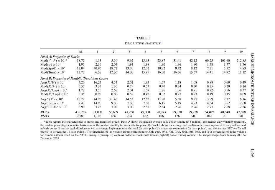
Table I reports descriptive statistics for traded stocks in panel A and for in-dividual transition orders in panel B. The first column reports statistics for all
MA
RK
ET
MIC
RO
STR
UC
TU
RE
INV
AR
IAN
CE
1369
TABLE I
DESCRIPTIVE STATISTICSa
All 1 2 3 4 5 6 7 8 9 10
Panel A: Properties of StocksMed(V · P)× 10−6 18�72 1�13 5�10 9�92 15�93 23�87 31�41 42�12 60�25 101�60 212�85Med(σ)× 102 1�93 2�16 2�04 1�94 1�98 1�90 1�86 1�80 1�78 1�77 1�76Med(Sprd)× 104 12�04 40�96 18�72 13�70 12�02 10�32 9�42 8�12 7�21 5�92 4�83Med(Turn)× 102 12�72 6�58 12�36 14�80 15�95 16�80 16�36 15�37 14�41 14�92 11�12
Panel B: Properties of Portfolio Transitions OrdersAvg(X/V )× 102 4�20 16�23 4�54 2�62 1�83 1�37 1�18 1�08 0�88 0�69 0�49Med(X/V )× 102 0�57 3�33 1�36 0�79 0�53 0�40 0�34 0�30 0�25 0�20 0�14Avg(X/Cap)× 104 1�72 3�55 2�68 2�04 1�59 1�26 1�06 0�91 0�72 0�56 0�37Med(X/Cap)× 104 0�35 0�98 0�80 0�58 0�42 0�32 0�27 0�23 0�19 0�15 0�09
AvgC(X)× 104 16�79 44�95 21�46 14�53 12�62 11�70 5�58 9�27 3�99 7�37 6�16Avg Comm×104 7�43 14�90 9�30 7�86 7�00 6�15 5�49 4�93 4�34 3�62 2�68Avg SEC fee × 105 2�90 3�26 3�02 3�00 2�85 2�84 2�76 2�76 2�73 2�68 2�56
#Obs 439,765 71,000 68,689 41,238 49,000 28,073 29,330 29,778 34,409 40,640 47,608#Stks 2,583 1,108 486 224 182 106 126 90 102 81 78
aTable reports the characteristics of stocks and transition orders. Panel A shows the median average daily dollar volume (in $ million), the median daily volatility (percent),the median percentage spread (in basis points), the median monthly turnover rate (in percent). Panel B shows the average and median order size (in percent of daily volume andin basis points of market capitalization) as well as average implementation shortfall (in basis points), the average commission (in basis points), and the average SEC fee for sellorders (in percent per 10 basis points). The thresholds of ten volume groups correspond to 30th, 50th, 60th, 70th, 75th, 80th, 85th, 90th, and 95th percentiles of dollar volumefor common stocks listed on the NYSE. Group 1 (Group 10) contains orders in stocks with lowest (highest) dollar trading volume. The sample ranges from January 2001 toDecember 2005.

1370 A. S. KYLE AND A. A. OBIZHAEVA
stocks in aggregate; the remaining ten columns report statistics for stocks inten dollar-volume groups. Instead of dividing the stocks into ten deciles withthe same number of stocks in each decile, volume break points are set at the30th, 50th, 60th, 70th, 75th, 80th, 85th, 90th, and 95th percentiles of trad-ing volume for the universe of stocks listed on the NYSE with CRSP sharecodes of 10 and 11. Group 1 contains stocks in the bottom 30th percentileof dollar trading volume. Group 10 approximately corresponds to the uni-verse of S&P 100 stocks. The top five groups approximately cover the uni-verse of S&P 500 stocks. Narrower percentile bands for the more active stocksmake it possible to focus on the stocks which are most important economically.For each month, the thresholds are recalculated and the stocks are reshuffledacross bins.
Panel A of Table I reports descriptive statistics for traded stocks. For theentire sample, the median daily volume is $18.72 million, ranging from $1.13million for the lowest volume group to $212.85 million for the highest volumegroup. The median volatility is 1.93 percent per day, ranging from 1.76 percentin the highest-volume decile to 2.16 in the lowest-volume decile. Since thereis so much more cross-sectional variation in dollar volume than in volatilityacross stocks, the variation in trading activity across stocks is related mostly tovariation in dollar volume. Trading activity differs by a factor of 150 betweenstocks in the lowest group and stocks in the highest group, and this variationcreates statistical power helpful in determining how transaction costs and ordersizes vary with trading activity.
The median quoted bid-ask spread, obtained from the transition data set, is12.04 basis points; its mean is 25.42 basis points. From lowest-volume group tohighest-volume group, the median spread declines monotonically from 40.96to 4.83 basis points, by a factor of 8�48. A back-of-the-envelope calculationbased on invariance suggests that spreads should decrease approximately by afactor of 1501/3 ≈ 5�31 from lowest- to highest-volume group. The differencebetween 5�31 and 8�48 is partially explained by differences in returns volatilityacross the volume groups and warrants further investigation. The monotonicdecline of almost one order of magnitude is potentially large enough to gener-ate significant statistical power in estimates of a bid-ask spread component oftransaction costs based on implementation shortfall.
Panel B of Table I reports properties of portfolio transition order sizes. Theaverage order size is 4�20% of average daily volume, declining monotonicallyacross the ten volume groups from 16�23% in the smallest group to 0�49%in the largest group, by a factor of 33�12. The median order is 0�57% of av-erage daily volume, also declining monotonically from 3�33% in the smallestgroup to 0�14% in the largest group, by a factor of 23�79. The invariance hy-pothesis implies that order sizes should decline by a factor of approximately1502/3 ≈ 28�23, a value which matches the data closely. The medians are muchsmaller than the means, indicating that distributions of order sizes are skewedto the right. We show below that the distribution of order sizes closely fits alog-normal.

MARKET MICROSTRUCTURE INVARIANCE 1371
The average trading cost (estimated based on implementation shortfall,as explained below) is 16�79 basis points per order, ranging from 44�95 ba-sis points in the lowest-volume group to 6�16 basis points in the highest-volume group. Invariance suggests that these costs should fall by a factor of1501/3 ≈ 5�31, somewhat smaller than the actual decline. The cost estimatesexclude commissions and SEC fees.7
One portfolio transition typically contains orders for dozens or hundredsof stocks. It typically takes several days to execute all of the orders. About60% of orders are executed during the first day of a portfolio transition. Sincetransition managers often operate under a cash-in-advance constraint—usingproceeds from selling stocks in a legacy portfolio to acquire stocks in a targetportfolio—sell orders tend to be executed slightly faster than buy orders (1�72days versus 1�85 days). In terms of dollar volume, about 41%, 23%, 15%, 7%,and 5% of dollar volume is executed on the first day through the fifth days,respectively. The two longest transitions in the sample were executed over 18and 19 business days. The time frame for a portfolio transition is usually setbefore its actual implementation begins.
4. EMPIRICAL TESTS BASED ON ORDER SIZES
Market microstructure invariance predicts that the distribution of W 2/3jt ·
Qjt/Vjt does not vary across stocks or time (see equation (8)). We test thesepredictions using data on portfolio transition orders, making the identifyingassumption that portfolio transition orders are proportional to bets.
Portfolio Transitions and Bets
Since bets are statistically independent intended orders, bets can be concep-tually difficult for researchers to observe. Consider, for example, a trader whomakes a decision on Monday to make one bet to buy 100,000 shares of stock,then implements the bet by purchasing 20,000 shares on Monday and 80,000shares on Thursday. To an econometrician, this one bet for 100,000 shares maybe difficult to distinguish from two bets for 20,000 shares and 80,000 shares,respectively. In the context of a portfolio transition, identifying a bet is eas-ier because the size of the order for 100,000 shares is known and recorded onMonday, even if the order is executed over several subsequent days.
Portfolio transition orders may not have a size distribution matching pre-cisely the size distribution of typical bets. Transition orders may be smaller
7The SEC fee represents a cost of about 0�29 basis points, which does not vary much acrossvolume groups. The average commission is 7�43 basis points, declining monotonically by a factorof 7�30 from 14�90 basis points for the lowest group to 2�68 basis points for the highest group.Since commissions may be negotiated for the entire transition, the allocation of commission coststo individual stocks is an accounting exercise with little economic meaning.

1372 A. S. KYLE AND A. A. OBIZHAEVA
than bets if transitions tend to liquidate a portion of an asset manager’s posi-tions or larger than bets if transitions liquidate the sum of bets made by theasset manager in the past. When both target and legacy portfolios hold longpositions in the same stock, the portfolio transition order may represent thedifference between two bets.
Let Xi denote the unsigned number of shares transacted in portfolio tran-sition order i, i = 1� � � � �439�765. The quantity Xi sums shares traded overmultiple days, excluding in-kind transfers.
We make the identifying assumption that, for some constant δ which doesnot vary across stocks with different characteristics such as volatility and trad-ing activity, the distribution of scaled portfolio transition orders δ ·Xi is thesame as the distribution of unsigned bets in the same stock at the same time,denoted |Q|. If δ = 1, the distribution of portfolio transition orders matchesthe distribution of bets. If the scaling constant δ were correlated with volatilityor trading activity, parameter estimates might be biased.
The Empirical Hypotheses of Invariance and Log-Normality for the SizeDistribution of Portfolio Transition Orders
Let Wi := Vi · Pi · σi and Wi := Vi · Pi · σi denote trading activity and bet ac-tivity, respectively, for the stock in transition order i. Under the identifying as-sumption that portfolio transition orders are proportional to bets, invarianceof bets implies invariance of portfolio transition orders. Specifically, replacingQjt withXi in equation (8) implies that the distribution of W 2/3
i ·Xi/Vi does notvary with stock characteristics such as volume, volatility, stock price, or marketcapitalization.
To facilitate intuitive interpretation of parameter estimates, we scale obser-vations by a hypothetical benchmark stock with price P∗ of $40 per share, dailyvolume V ∗ of one million shares, and volatility σ∗ of 2% per day, implyingW ∗ = 40 × 106 · 0�02. This benchmark stock would belong to the bottom tercileof S&P 500 (volume group 7 in Table I).
Combining invariance of portfolio transition orders with equations (1)and (2) to convert the bet activity variables Wi and Vi into trading activity vari-ables Wi and Vi and taking logs, invariance implies the empirically testable re-lationship
ln[(
Wi
W ∗
)2/3
· Xi
Vi
]= ln[q] + εi�(23)
Under the identifying assumptions that the volume multiplier ζ, the volatilitymultiplier ψ, and the deflator δ do not vary across observations, ln[q] is aninvariant constant ln[q] = E{ln[|Q∗|/V ∗]} − ln[δ] and εi is a zero-mean error
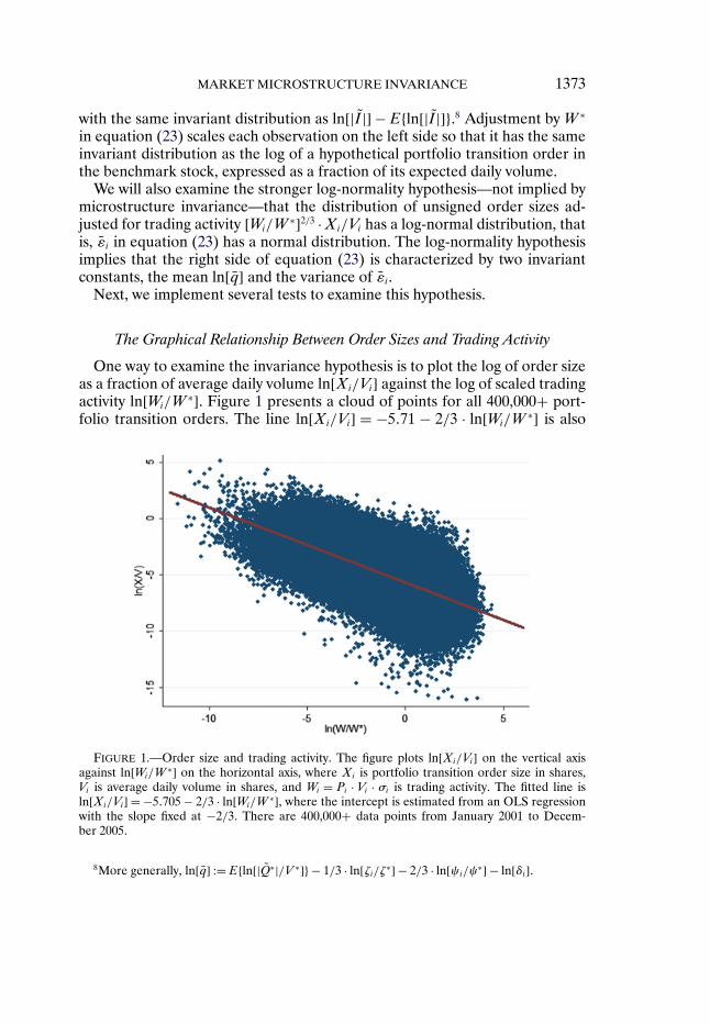
MARKET MICROSTRUCTURE INVARIANCE 1373
with the same invariant distribution as ln[|I|] −E{ln[|I|]}.8 Adjustment by W ∗
in equation (23) scales each observation on the left side so that it has the sameinvariant distribution as the log of a hypothetical portfolio transition order inthe benchmark stock, expressed as a fraction of its expected daily volume.
We will also examine the stronger log-normality hypothesis—not implied bymicrostructure invariance—that the distribution of unsigned order sizes ad-justed for trading activity [Wi/W
∗]2/3 ·Xi/Vi has a log-normal distribution, thatis, εi in equation (23) has a normal distribution. The log-normality hypothesisimplies that the right side of equation (23) is characterized by two invariantconstants, the mean ln[q] and the variance of εi.
Next, we implement several tests to examine this hypothesis.
The Graphical Relationship Between Order Sizes and Trading Activity
One way to examine the invariance hypothesis is to plot the log of order sizeas a fraction of average daily volume ln[Xi/Vi] against the log of scaled tradingactivity ln[Wi/W
∗]. Figure 1 presents a cloud of points for all 400,000+ port-folio transition orders. The line ln[Xi/Vi] = −5�71 − 2/3 · ln[Wi/W
∗] is also
FIGURE 1.—Order size and trading activity. The figure plots ln[Xi/Vi] on the vertical axisagainst ln[Wi/W
∗] on the horizontal axis, where Xi is portfolio transition order size in shares,Vi is average daily volume in shares, and Wi = Pi · Vi · σi is trading activity. The fitted line isln[Xi/Vi] = −5�705 − 2/3 · ln[Wi/W
∗], where the intercept is estimated from an OLS regressionwith the slope fixed at −2/3. There are 400,000+ data points from January 2001 to Decem-ber 2005.
8More generally, ln[q] :=E{ln[|Q∗|/V ∗]} − 1/3 · ln[ζi/ζ∗] − 2/3 · ln[ψi/ψ∗] − ln[δi].

1374 A. S. KYLE AND A. A. OBIZHAEVA
shown for comparison. The slope of this line is fixed at −2/3, as implied by in-variance; the intercept, estimated from an OLS regression, is the sample mean.On the horizontal axis, zero represents the log of trading activity in the bench-mark stock; on the vertical axis, zero represents orders for 100% of expecteddaily volume. The shape of the “super-cloud” conforms well with the invari-ance hypothesis in that the slope of −2/3 is close to the shape of the plottedpoints and there is only little evidence of heteroscedasticity.
Log-Normal Order Size Distribution for Volume and Volatility Groups
When the portfolio transition orders are sorted into different groups basedon characteristics such as dollar volume, volatility, stock price, and turnover,the joint hypotheses of invariance and log-normality imply that the means andvariances of ln[(Wi/W
∗)2/3 ·Xi/Vi] for each group should match the mean andvariance of the pooled sample. The pooled sample mean of ln[(Wi/W
∗)2/3 ·Xi/Vi] is −5�71; the pooled sample variance is 2�53. The pooled sample mean isan estimate of ln[q]; the pooled sample variance is an estimate of the varianceof the error εi.9
To examine this hypothesis visually, we plot the empirical distributions ofthe left side of equation (23), ln[(Wi/W
∗)2/3 ·Xi/Vi], for selected volume andvolatility groups. As before, we define ten dollar-volume groups with thresh-olds corresponding to the 30th, 50th, 60th, 70th, 75th, 80th, 85th, 90th, and95th percentiles of NYSE dollar volume. We define five volatility groups withthresholds corresponding to the 20th, 40th, 60th, and 80th percentiles of re-turns standard deviation for NYSE stocks. On each plot, we superimpose thebell-shaped density function N(−5�71�2�53) matching the mean and varianceof the pooled sample.
Figure 2 shows plots of the empirical distributions of ln[(Wi/W∗)2/3 ·Xi/Vi]
for volume groups 1, 4, 7, 9, and 10 and for volatility groups 1, 3, and 5. Consis-tent with the invariance hypothesis, these fifteen distributions of W -adjustedorder sizes are all visually strikingly similar to the superimposed normal dis-tribution. Results for the remaining 35 subgroups also look very similar andtherefore are not presented in this paper. The visual similarity of the distri-butions is reflected in the similarity of their first four moments. For the 15volume-volatility groups, the means range from −6�03 to −5�41, close to themean of −5�71 for the pooled sample. The variances range from 2�23 to 2�90,also close to the variance of 2�53 for the pooled sample. The skewness rangesfrom −0�21 to 0�10, close to skewness of zero for the normal distribution. Thekurtosis ranges from 2�73 to 3�38, also close to the kurtosis of 3 for a nor-mal random variable. These results suggest that it is reasonable to assumethat unsigned order sizes have a log-normal distribution. Scaling order sizes
9There is not much difference in the distributions of buy and sell orders. For buy orders, themean is −5�70 and the variance is 2�51; for sell orders, the mean is −5�71 and the variance is 2�55.

MA
RK
ET
MIC
RO
STR
UC
TU
RE
INV
AR
IAN
CE
1375
FIGURE 2.—Invariant order size distribution. Figure shows distributions of ln[X/V ] + 2/3 · ln[Wi/W∗] for stocks sorted into 10 volume groups
and 5 volatility groups (only volume groups 1, 4, 7, 9, 10 and volatility groups 1, 3, 5 are reported).Xi is an order size in shares, Vi is the average dailyvolume in shares, and Wi is the trading activity. The thresholds of ten volume groups correspond to 30th, 50th, 60th, 70th, 75th, 80th, 85th, 90th,and 95th percentiles of dollar volume for common stocks listed on the NYSE. Volume group 1 (group 10) contains orders in stocks with lowest(highest) dollar volume. The thresholds of five volatility groups correspond to 20th, 40th, 60th, and 80th percentiles for common NYSE-listedstocks. Volatility group 1 (group 5) has stocks with the lowest (highest) volatility. Each subplot also shows the number of observations (N), themean (m), the variance (v), the skewness (s), and the kurtosis (k) for depicted distribution. The normal distribution with the common mean of−5�71 and variance of 2�54 is imposed on each subplot. The common mean and variance are calculated as the mean and variance of distributionover the entire sample. The sample ranges from January 2001 to December 2005.
1376 A. S. KYLE AND A. A. OBIZHAEVA
by [Wi/W∗]2/3, as implied by the invariance hypothesis, adjusts the means of
the distributions so that they visually appear to be similar.Despite the visual similarity, a Kolmogorov–Smirnov test rejects the hypoth-
esis that all fifty empirical distributions are generated from the same normaldistribution. The standard deviation of the means across bins is larger thanimplied by a common normal distribution. Microstructure invariance does notdescribe the data perfectly, but it makes a good benchmark from which themodest deviations seen in these plots can be investigated in future research.
Figure 3 further examines log-normality by focusing on the tails of the distri-butions of portfolio transition orders. For each of the five volume groups 1, 4,7, 9, and 10, panel A shows quantile-quantile plots of the empirical distributionof ln[(Wi/W
∗)2/3 ·Xi/Vi] versus a normal distribution with the same mean andvariance. The more similar these empirical distributions are to a normal distri-bution, the closer the plots should be to the 45-degree line. Panel B shows logsof ranks based on scaled order sizes. Under the hypothesis of log-normality,the right tail should be quadratic. A straight line in the right tail would implya power law. Both panels show that the empirical distributions are similar to anormal distribution, except in the far right and left tails.
In panel A, the smallest orders in the left tails tend to be smaller than impliedby a normal distribution. These observations are economically insignificant.Most of them represent one-share transactions in low-price stocks (perhapsthe result of coding errors in the data). There are too few such orders to havea meaningful effect on our statistical results.
In panel A, the largest orders in the right tails are much more importanteconomically. On each subplot, a handful of positive outliers (out of 400,000+observations) do not appear to fit a normal distribution. The largest orders inlow-volume stocks appear to be smaller than implied by a normal distribution,and the largest orders in high-volume stocks appear to be larger than impliedby a normal distribution.
The finding that the largest orders in low-volume stocks are smaller thanimplied by a log-normal may be explained by reporting requirements. Whenan owner acquires more than 5% of the shares of a publicly traded company,the SEC requires information to be reported on Schedule 13D. To avoid re-porting requirements, large institutional investors may intentionally acquirefewer shares when intended holdings would otherwise exceed the 5% report-ing threshold. Indeed, all 400,000+ portfolio transition orders are for amountssmaller than 4.5% of shares outstanding. A closer examination reveals that thefive largest orders for low-volume stocks account for about 2%, 3%, 4%, 4%,and 4% of shares outstanding, respectively, just below the 5% threshold. Thelargest order in high-volume stocks is for only about 1% of shares outstanding.
To summarize, we conclude that the distribution of portfolio transition or-der sizes appears to conform closely to—but not exactly to—the invariancehypothesis. Furthermore, the distribution of order sizes appears to be similarto—but not exactly equal to—a log-normal.

MA
RK
ET
MIC
RO
STR
UC
TU
RE
INV
AR
IAN
CE
1377
FIGURE 3.—Invariant order size distribution. Panel A shows quantile-quantile plots of empirical distributions of ln[Xi/Vi] + 2/3 · ln[Wi/W∗]
and a normal distribution for stocks sorted into 10 volume groups (only volume groups 1, 4, 7, 9, 10 are reported). Panel B depicts the logarithm ofranks based on that distribution. The ten volume groups are based on average dollar trading volume with thresholds corresponding to 30th, 50th,60th, 70th, 75th, 80th, 85th, 90th, and 95th percentiles of the dollar volume for common NYSE-listed stocks. Volume group 1 (group 10) has stockswith the lowest (highest) trading volume. Each subplot shows the number of observations (N), the mean (m), the variance (v), the skewness (s),and the kurtosis (k) of a depicted distribution. There are 400,000+ data points. The sample ranges from January 2001 to December 2005.

1378 A. S. KYLE AND A. A. OBIZHAEVA
OLS Estimates of Order Size
The order size predictions from equation (23) can also be tested using asimple log-linear OLS regression
ln[Xi
Vi
]= ln[q] + α0 · ln
[Wi
W ∗
]+ εi�(24)
Invariance of bets implies α0 = −2/3.To adjust standard errors of OLS estimates of α0 for positive contempora-
neous correlation in transition order sizes across different stocks, the 439,765observations are pooled by week over the 2001–2005 period into 4,389 clustersacross 17 industry categories. The double clustering by weeks and industriesconservatively adjusts standard errors for large portfolio transitions that mayinvolve hundreds of relatively large orders, executed during the course of aweek and potentially concentrated in particular industries.10
Table II presents estimates for the OLS coefficients in equation (24). Thefirst column of the table reports the results of a regression pooling all the data.The four other columns in the table report results for four separate OLS re-gressions in which the parameters are estimated separately for NYSE Buys,NYSE Sells, NASDAQ Buys, and NASDAQ Sells.
For the entire sample, the estimate for α0 is α0 = −0�62 with standard errorof 0�009. Economically, the point estimate for α0 is close to the value −2/3 pre-dicted by the invariance hypothesis, but the hypothesis α0 = −2/3 is stronglyrejected (F = 25�31, p< 0�0001) because the standard error is very small.
When the sample is broken down into NYSE Buys, NYSE Sells, NASDAQBuys, and NASDAQ Sells, it is interesting to note that the estimated coeffi-cients for buy orders, −0�63 for NYSE and −0�71 for NASDAQ, are closerto −2/3 than the coefficients for sell orders, −0�59 for both NYSE and NAS-DAQ. Since portfolio transitions tend to be applied to long-only portfolios, sellorders tend to represent liquidations of past bets. If the size distribution of sellorders depends on past values of volume and volatility—not current values—there is an errors-in-variables problem related to current trading activity beingused as a noisy version of past trading activity. This will bias the absolute valuesof coefficient estimates downward, consistent with the absolute values of thecoefficient estimates for NYSE and NASDAQ sell orders being less than 2/3.
10A potential econometric issue with the log-linear specification in equation (24) is that takingthe log of order size as a fraction of average daily volume may create large negative outliersfrom tiny, economically meaningless orders, with an inordinately large influence on coefficientestimates. Since we have shown above that the shape of the distribution of scaled order sizesclosely matches a log-normal, these tiny orders are expected to have only a negligible distortingeffect on estimates.

MARKET MICROSTRUCTURE INVARIANCE 1379
TABLE II
OLS ESTIMATES OF ORDER SIZEa
NYSE NASDAQ
All Buy Sell Buy Sell
ln[q] −5�67 −5�68 −5�63 −5�75 −5�65(0�017) (0�023) (0�018) (0�035) (0�032)
α0 −0�62 −0�63 −0�59 −0�71 −0�59(0�009) (0�011) (0�008) (0�019) (0�015)
R2 0�3167 0�2587 0�2646 0�4298 0�3542Q∗/V ∗ · δ−1 × 10⁴ 34�62 34�14 35�98 31�80 34�78#Obs 439,765 131,530 150,377 69,871 87,987
aTable presents the estimates ln[q] and α0 for the regression
ln[XiVi
]= ln[q] + α0 · ln
[WiW ∗
]+ εi�
Each observation corresponds to transition order i with order size Xi , pre-transition price Pi , expected daily volumeVi , expected daily volatility σi , trading activity Wi . The parameter q is the measure of order size such that for δ= 1,Q∗/V ∗ ·δ−1 ×10⁴ measures the median bet size for the benchmark stock, in basis points of average daily volume. Thebenchmark stock has daily volatility of 2%, share price of $40, and daily volume of one million shares. The standarderrors are clustered at weekly levels for 17 industries and shown in parentheses. The sample ranges from January 2001to December 2005.
Quantile Estimates of Order Sizes
Table A.I in the Supplemental Material presents quantile regression resultsfor equation (24) based on the 1st (smallest orders), 5th, 25th, 50th, 75th, 95th,and 99th percentiles (largest orders). The corresponding quantile estimatesfor α0 are −0�65, −0�64, −0�61, −0�62, −0�61, −0�64, and −0�63, respectively.Although the hypothesis α0 = −2/3 is rejected due to small standard errors,all quantile estimates are economically close to the value of −2/3 predicted bythe invariance hypothesis.
Model Calibration and Its Economic Interpretation
Under the invariance-of-bets and log-normality hypotheses, we can calibratethe distribution of bet sizes by imposing the restriction α0 = −2/3 on equa-tion (24). Thus, only the constant term in the regression needs to be estimated.
The results of this calibration exercise are presented in Table III. The esti-mated constant term, −5�71, is the previously reported sample mean of ln[q] inequation (23). The mean squared error, 2�53, is the previously reported samplevariance of εi in equation (23).
The R2 (with zero degrees of freedom) is 0�3149; the log of trading activityln[Wi/W
∗], with the coefficient α0 = −2/3 imposed by invariance, explains asignificance percentage of the variation of order size as a fraction of volumeXi/Vi.
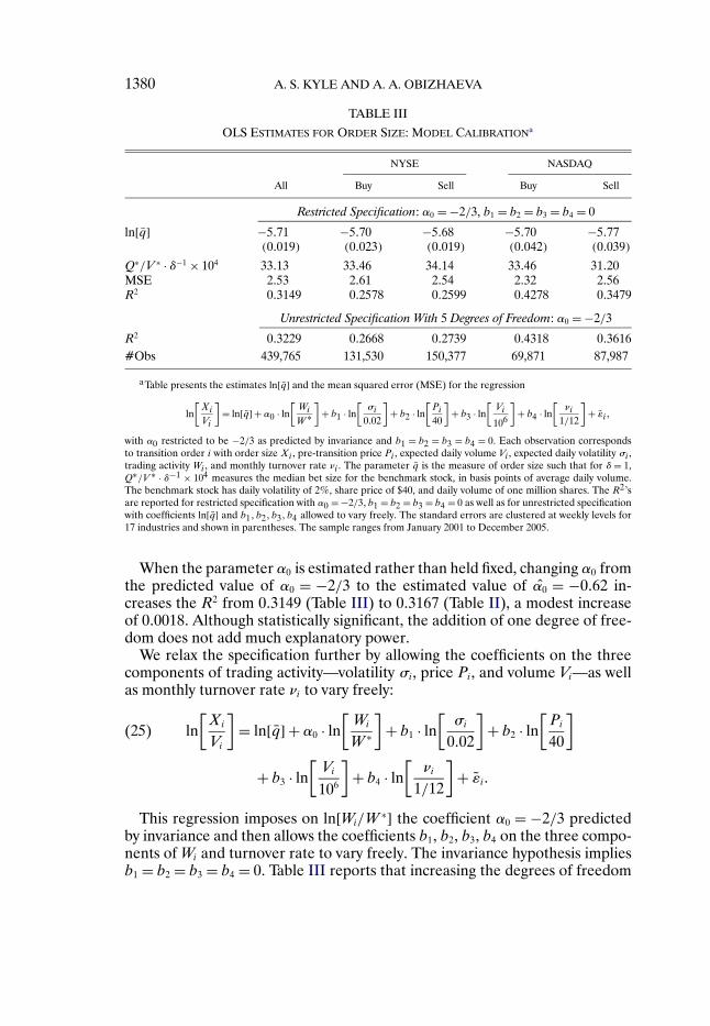
1380 A. S. KYLE AND A. A. OBIZHAEVA
TABLE III
OLS ESTIMATES FOR ORDER SIZE: MODEL CALIBRATIONa
NYSE NASDAQ
All Buy Sell Buy Sell
Restricted Specification: α0 = −2/3, b1 = b2 = b3 = b4 = 0
ln[q] −5�71 −5�70 −5�68 −5�70 −5�77(0�019) (0�023) (0�019) (0�042) (0�039)
Q∗/V ∗ · δ−1 × 10⁴ 33�13 33�46 34�14 33�46 31�20MSE 2�53 2�61 2�54 2�32 2�56R2 0�3149 0�2578 0�2599 0�4278 0�3479
Unrestricted Specification With 5 Degrees of Freedom: α0 = −2/3
R2 0�3229 0�2668 0�2739 0�4318 0�3616#Obs 439,765 131,530 150,377 69,871 87,987
aTable presents the estimates ln[q] and the mean squared error (MSE) for the regression
ln[XiVi
]= ln[q] + α0 · ln
[WiW ∗
]+ b1 · ln
[σi
0�02
]+ b2 · ln
[Pi40
]+ b3 · ln
[Vi
106
]+ b4 · ln
[νi
1/12
]+ εi�
with α0 restricted to be −2/3 as predicted by invariance and b1 = b2 = b3 = b4 = 0. Each observation correspondsto transition order i with order size Xi , pre-transition price Pi , expected daily volume Vi , expected daily volatility σi ,trading activity Wi , and monthly turnover rate νi . The parameter q is the measure of order size such that for δ = 1,Q∗/V ∗ · δ−1 × 10⁴ measures the median bet size for the benchmark stock, in basis points of average daily volume.The benchmark stock has daily volatility of 2%, share price of $40, and daily volume of one million shares. The R2’sare reported for restricted specification with α0 = −2/3� b1 = b2 = b3 = b4 = 0 as well as for unrestricted specificationwith coefficients ln[q] and b1� b2� b3� b4 allowed to vary freely. The standard errors are clustered at weekly levels for17 industries and shown in parentheses. The sample ranges from January 2001 to December 2005.
When the parameter α0 is estimated rather than held fixed, changing α0 fromthe predicted value of α0 = −2/3 to the estimated value of α0 = −0�62 in-creases the R2 from 0�3149 (Table III) to 0�3167 (Table II), a modest increaseof 0�0018. Although statistically significant, the addition of one degree of free-dom does not add much explanatory power.
We relax the specification further by allowing the coefficients on the threecomponents of trading activity—volatility σi, price Pi, and volume Vi—as wellas monthly turnover rate νi to vary freely:
ln[Xi
Vi
]= ln[q] + α0 · ln
[Wi
W ∗
]+ b1 · ln
[σi
0�02
]+ b2 · ln
[Pi
40
](25)
+ b3 · ln[Vi
106
]+ b4 · ln
[νi
1/12
]+ εi�
This regression imposes on ln[Wi/W∗] the coefficient α0 = −2/3 predicted
by invariance and then allows the coefficients b1, b2, b3, b4 on the three compo-nents of Wi and turnover rate to vary freely. The invariance hypothesis impliesb1 = b2 = b3 = b4 = 0. Table III reports that increasing the degrees of freedom

MARKET MICROSTRUCTURE INVARIANCE 1381
from one to four increases the R2 of the regression from 0�3167 to 0�3229, anincrease of 0�0062. Although statistically significant, the improvement in R2 isagain modest. Invariance explains much—but not quite all—of the variation inportfolio transition order size across stocks that can be explained by all fourvariables.
The point estimates for the coefficient on volatility of b1 = 0�42, the coeffi-cient on price of b2 = 0�24, the coefficient on share volume of b3 = 0�06, thecoefficient on turnover rate of b4 = −0�18 are all statistically significant, withstandard errors of 0�040, 0�019, 0�010, and 0�015, respectively (see Table A.IIin the Supplemental Material). The coefficients on volatility and price are sig-nificantly positive, indicating that order size—as a fraction of average dailyvolume—does not decrease with increasing volatility and price as fast as pre-dicted by the invariance hypothesis. The statistically significant positive coef-ficient on volume may be partially offset by a statistically significant negativecoefficient on turnover rate.
Discussion
The documented log-normality of bet size is strikingly different from thetypical assumptions of microstructure models, where innovations in order flowfrom noise traders are distributed as a normal, not a log-normal or power law.Although normal random variables are a convenient modeling device—theyallow conditional expectations to be linear functions of underlying jointly nor-mally distributed variables—their implications are qualitatively very different.
The estimated log-mean of −5�71 implies that a median portfolio transitionorder size is equal to 0�33% of expected daily volume for the benchmark stock,since exp(−5�71) ≈ 0�0033. The estimated log-variance of 2�53 implies that aone standard deviation increase in order size is a factor of 4�90 for all stocks,since exp(2�531/2)≈ 4�90.
We next explain why the log-variance of 2�53 also implies that a large fractionof trading volume and an even larger fraction of returns variance come fromlarge bets.
Let η(z) and N(z) denote the PDF and CDF, respectively, of a standard-ized normal distribution. Define F(z�p) by F(z�p) := ∫ ∞
z=z exp(p · √2�53 ·
z) · η(z) · dz. It is easy to show that F(z�p) = exp(p2 · 2�53/2) · (1 −N(z −p ·√2�53)). This implies that the fraction of the pth moment of order size aris-ing from bets greater than z standard deviations above the log-mean is givenby F(z�p)/F(−∞�p)= 1 −N(z−p · √2�53).
Plugging p = 1, we find that bets larger than z standard deviations abovethe log-mean (median) generate a fraction of total trading volume given by1 − N(z − √
2�53). Bets larger than the 50th percentile generate 94�41% oftrading volume (z = 0). Bets larger than
√2�53 standard deviations above the

1382 A. S. KYLE AND A. A. OBIZHAEVA
log-mean (median) bet size—that is, the largest 5�39% of bets—generate 50%of trading volume (z = √
2�53).Plugging p = 2, we find that bets larger than z standard deviations above
the log-mean bet size contribute a fraction of total returns variance given by1 − N(z − 2 · √
2�53) under the assumption that the contribution of bets toprice variance is proportional to their squared size (implied by linear price im-pact). Bets greater than the 50th percentile generate 99�93% of returns vari-ance (z = 0). Bets larger than 2 · √
2�53 = 3�18 standard deviations above thelog-mean—that is, the largest 0�07% of bets—generate 50% of returns vari-ance (z = 2 · √2�53).
Under the assumptions ζ/2 = ψ = δ = 1 (stronger than our identifying as-sumptions), the estimates of mean and variance imply that the benchmarkstock has about 85 bets per day for each of the 252 trading days in a calen-dar year. These estimates then imply that the 1,155 largest bets out of 21,420bets generate approximately half of the trading volume during one year, andthe 15 largest bets generate approximately half of returns variance during oneyear.
Rare large bets may not only account for a significant percentage of returnsvariance but may also account for some of the stochastic time-series variationin volatility. We conjecture that the pattern of short-term volatility associatedwith execution of rare large bets may depend on the speed with which suchbets are executed. As discussed by Kyle and Obizhaeva (2016a), large marketdisturbances such as the stock market crashes of 1929 and 1987, the liquidationof Jerome Kerviel’s rogue trades by Société Générale, and the flash crash ofMay 6, 2010, could have been induced by execution of gigantic bets.
Another implication of log-normality may be a greater kurtosis in the em-pirical distribution of price changes than a normal distribution would suggest.Given the estimated log-variance of 2�53, it can be shown that the excess kur-tosis of one bet has the enormous value of about exp(4 · 2�53), or approxi-mately 22,000.
Invariance implies a different way of thinking about trading data from that inthe time-change literature, which goes back to Mandelbrot and Taylor (1967)and Clark (1973). Mandelbrot and Taylor (1967) began with the intuition thatthe distribution of price changes is a stable distribution, that is, a distributionwith the property that a linear combination of two independent random vari-ables has the same shape, up to location and scale parameters. Since it hasfatter tails than a normal distribution, it is confined to be a stable Pareto dis-tribution. Following this line of research, the econophysics literature—such asGopikrishnan, Meyer, Amaral, and Stanley (2005), Plerou et al. (2000), andGabaix et al. (2006)—estimates different power laws for the probability dis-tributions of different variables and searches for price-formation models con-sistent with those distributions. Whether order size follows a power law or alog-normal distribution is an interesting question for future research.

MARKET MICROSTRUCTURE INVARIANCE 1383
Clark (1973) suggested as an alternative hypothesis that the distribution ofdaily price changes is subordinated to a normal distribution with a time clocklinked to a log-normally distributed trading volume. The log-normal distribu-tion is neither stable nor infinitely divisible; the sum of random variables withindependent log-normal distributions is not log-normal. Thus, if daily pricechanges can be described by Clark’s hypothesis, neither half-day price changesnor weekly price changes will be described by the same hypothesis.
In some sense, our approach seems to be closer to Mandelbrot and Taylor(1967), who imagined orders of different sizes arriving in the market, with busi-ness time linked to their arrival rates rather than to trading volume.
Empirical regularities similar to those implied by invariance can be inferredfrom the previous literature. Bouchaud, Farmer, and Lillo (2009) reported, forexample, that the number of TAQ prints per day is proportional to market cap-italization raised to powers between 0�44 to 0�86. Under the assumption thatvolatility and turnover rates are stable across stocks as shown in Table I, themidpoint 0�65 of that interval is close to the value of 2/3 implied by invariancefor the number of bets per day.
The log-normality of bet size may be related to the log-normality of assetsunder management for financial firms. Schwarzkopf and Farmer (2010) studiedthe size of U.S. mutual funds and found that its distribution closely conformsto a log-normal with log-variance of about 2�50, similar to our estimates of log-variance for portfolio transition orders. Their annual estimates of log-varianceare stable during the twelve years from 1994 to 2005, ranging from 2�43 to 2�59.For years 1991, 1992, and 1993, the log-variance estimates of 1�51, 1�98, and2�09 are slightly lower, probably because many observations are missing fromthe CRSP U.S. mutual funds data set for those years.
As discussed by Aitchison and Brown (1957), log-normal distributions canbe found in many areas of natural science. For example, Kolmogorov (1941b)proved mathematically that the probability distribution of the sizes of particlesunder fragmentation converges over time to a log-normal.
5. EMPIRICAL TESTS BASED ON TRANSACTION COSTS
To examine statistically whether transaction costs conform to the predictionsof market microstructure invariance in equation (16), we use the concept ofimplementation shortfall developed by Perold (1988). Specifically, we estimatecosts by comparing the average execution prices of portfolio transition orderswith closing prices the evening before any portfolio transition orders begin tobe executed. Our tests measure implicit transaction costs resulting from bid-ask spreads and market impact; they exclude explicit transaction costs such ascommissions and fees.

1384 A. S. KYLE AND A. A. OBIZHAEVA
Portfolio Transitions and Implementation Shortfall
In portfolio transitions, quantities to be traded are known precisely beforetrading begins, these quantities are recorded accurately, and all intended quan-tities are executed. In other trading situations, quantities intended to be tradedmay not be recorded accurately, and orders may be canceled or quantities maybe revised in response to price movements after trading begins. When ordersare canceled after prices move in an unfavorable direction or when order size isincreased after prices move in a favorable direction, implementation shortfallmay dramatically underestimate actual transaction costs. Portfolio transitionsdata are not subject to these concerns.
Portfolio transition trades are unlikely to be based on short-lived privateinformation about specific stocks because decisions to undertake portfoliotransitions and their timing likely result from regularly scheduled meetings ofinvestment committees and boards of plan sponsors, not from fast-breakingprivate information in the hands of fund managers. Transaction-cost estimatesare therefore unlikely to be biased upward as a result of short-lived privateinformation being incorporated into prices while orders are being executed.
These properties of portfolio transitions are not often shared by other data.Consider a data set built up from trades by a mutual fund, a hedge fund, ora proprietary trading desk at an investment bank. In such samples, the inten-tions of traders may not be recorded in the data set. For example, a data setmight time-stamp a record of a trader placing an order to buy 100,000 sharesof stock but not time-stamp a record of the trader’s actual intention to buyanother 200,000 shares after the first 100,000 shares are bought. Furthermore,trading intentions may not coincide with realized trades because the traderchanges his mind as market conditions change. Indeed, traders often conditiontheir trading strategies on prices by using limit orders or canceling orders, thushard-wiring into their strategies a selection bias problem for using such datato estimate transaction costs. The dependence of actually traded quantities onprices usually makes it impossible to use implementation shortfall in a mean-ingful way to estimate market depth and bid-ask spreads from data on tradesonly. Portfolio transitions data are particularly well suited for using implemen-tation shortfall to measure transaction costs because portfolio transitions dataavoid these sources of statistical bias. These selection-bias issues are discussedin more detail by Obizhaeva (2012).
The Empirical Hypotheses of Invariance and a Power Function Specification forTransaction Costs
For each unsigned transition order Xi, let IBS�i denote a buy-sell indicatorvariable which is equal to +1 for buy orders and −1 for sell orders. For tran-sition order i, let Ci denote the expected transaction cost as a fraction of thevalue transacted. Let Si denote the actual implementation shortfall, defined bySi = IBS�i · (Pex�i − Pi)/Pi, where Pex�i is the average execution price of order
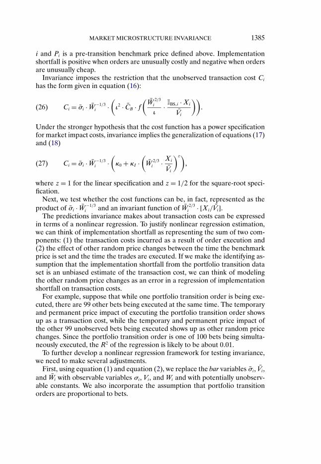
MARKET MICROSTRUCTURE INVARIANCE 1385
i and Pi is a pre-transition benchmark price defined above. Implementationshortfall is positive when orders are unusually costly and negative when ordersare unusually cheap.
Invariance imposes the restriction that the unobserved transaction cost Cihas the form given in equation (16):
Ci = σi · W −1/3i ·
(ι2 · CB · f
(W 2/3i
ι· IBS�i ·Xi
Vi
))�(26)
Under the stronger hypothesis that the cost function has a power specificationfor market impact costs, invariance implies the generalization of equations (17)and (18)
Ci = σi · W −1/3i ·
(κ0 + κI ·
(W 2/3i · Xi
Vi
)z)�(27)
where z = 1 for the linear specification and z = 1/2 for the square-root speci-fication.
Next, we test whether the cost functions can be, in fact, represented as theproduct of σi · W −1/3
i and an invariant function of W 2/3i · [Xi/Vi].
The predictions invariance makes about transaction costs can be expressedin terms of a nonlinear regression. To justify nonlinear regression estimation,we can think of implementation shortfall as representing the sum of two com-ponents: (1) the transaction costs incurred as a result of order execution and(2) the effect of other random price changes between the time the benchmarkprice is set and the time the trades are executed. If we make the identifying as-sumption that the implementation shortfall from the portfolio transition dataset is an unbiased estimate of the transaction cost, we can think of modelingthe other random price changes as an error in a regression of implementationshortfall on transaction costs.
For example, suppose that while one portfolio transition order is being exe-cuted, there are 99 other bets being executed at the same time. The temporaryand permanent price impact of executing the portfolio transition order showsup as a transaction cost, while the temporary and permanent price impact ofthe other 99 unobserved bets being executed shows up as other random pricechanges. Since the portfolio transition order is one of 100 bets being simulta-neously executed, the R2 of the regression is likely to be about 0�01.
To further develop a nonlinear regression framework for testing invariance,we need to make several adjustments.
First, using equation (1) and equation (2), we replace the bar variables σi, Vi,and Wi with observable variables σi, Vi, and Wi and with potentially unobserv-able constants. We also incorporate the assumption that portfolio transitionorders are proportional to bets.

1386 A. S. KYLE AND A. A. OBIZHAEVA
Second, since we want the error in our regression of implementation short-fall on transaction costs to be positive when the stock price is moving up andnegative when the stock price is moving down, we multiply both the implemen-tation shortfall Si and the transaction-cost function C(Xi) by the buy-sell indi-cator. The regression specification can be then written IBS�i · Si = IBS�i ·Ci + εi.Note that IBS�i · Si = (Pex�i − Pi)/Pi since I
2BS�i = 1. This gives us a nonlinear
regression of the form
IBS�i · Si = IBS�i ·[ψ
ψ∗
]2/3[ζ
ζ∗
]1/3[σi
σ∗
][Wi
W ∗
]−1/3
· f (Ii · δ−1)/L∗ + εi�(28)
where Ii := φ−1 · (Wi/W∗)2/3 ·Xi/Vi, with invariant constant φ obtained from
equation (8) and illiquidity measure for the benchmark stock 1/L∗ := ι2 · CB ·σ∗ · [W ∗]−1/3 obtained from equation (15).11 Note that f (I · δ−1)/L∗ denotesthe invariant cost function for the benchmark stock, expressed as a fraction ofnotional value, similar to equation (14).
Third, we make another technical adjustment. Since Wi, Xi, and Vi are ob-servable, the quantityφ ·Ii is observable. The quantity Ii itself in equation (28),however, is not observable because the constant φ is defined in terms of po-tentially unobservable constants ι, δ, ψ, and ζ. To estimate the nonlinear re-gression equation (28), we substitute for f (·) a different function f ∗(·) definedby f ∗(x) = (ψ/ψ∗)2/3 · (ζ/ζ∗)1/3 · f (φ−1δ−1x). Using x = φ · Ii, the right sideof equation (28) becomes a simpler expression in terms of observable data,with various potentially unobserved constants incorporated into the definitionof f ∗, whose functional form is to be estimated from the data. Under the iden-tifying assumptions ψ = ψ∗ and ζ = ζ∗, we have f ∗(φIi) = f (Ii · δ−1), whereφ · Ii := (Wi/W
∗)2/3 ·Xi/Vi is observable. The unobserved constants hidden inφ affect the economic interpretation of the scaling of the estimated functionalform for f ∗(·), but they do not otherwise affect the estimation itself. If ζi, ψi,and δi are not constants, but instead are correlated with variables like Wi, thiswould raise problems of statistical bias in our parameter estimates.
Fourth, the variance of errors in the regression is likely to be proportional insize to the variance of returns and the execution horizon. On average, portfo-lio transition orders tend to be executed in about one day. To correct for het-eroscedasticity resulting from differences in returns volatility, we divide boththe right and left sides by returns volatility σi/σ∗, where σ∗ = 0�02. Indeed,this adjustment makes the root mean squared error of the resulting regressionapproximately equal to 0�02.
Fifth, to control for the economically and statistically significant influencethat general market movements have on implementation shortfall, we add theCRSP value-weighted market return Rmkt�i on the first day of the transition
11More specifically, φ := δ−1ιψ−2/3(ζ/2)−1/3(W ∗)−2/3.

MARKET MICROSTRUCTURE INVARIANCE 1387
to the right side of the regression equation. To the extent that portfolio tran-sition orders are sufficiently large to move the entire U.S. stock market, thisadjustment will result in understated transaction costs by measuring only theidiosyncratic component of transaction costs. It is an interesting subject for fu-ture research to investigate how large trades in multiple stocks affect generalmarket movements.
Upon making these two changes and using the definition of f ∗(·), regressionequation (28) becomes
IBS�i ·Si · (0�02)σi
= βmkt ·Rmkt�i · (0�02)σi
+ IBS�i ·[Wi
W ∗
]α·f ∗(φIi)/L∗ + εi�(29)
where invariance implies α = −1/3. One of our tests is designed to examinethis prediction.
Scaling by W ∗ makes the function f ∗(φIi)/L∗ in equation (29) measurethe transaction cost for the benchmark stock in terms of the observable valueφIi. Although invariance itself does not specify a function form for f ∗(·)/L∗,the regression places strong cross-sectional restrictions on the shape of thetransaction-cost function. In addition to the restriction α = −1/3, it requiresthat the same function f ∗(φIi)/L∗ with φIi = (Wi/W
∗)2/3 ·Xi/Vi for order i beused for all stocks. We test this prediction as well.
We do not undertake separate estimates of transaction-cost parameters forinternal crosses, external crosses, and open market transactions. Such esti-mates would be difficult to interpret due to selection bias resulting from tran-sition managers optimally choosing trading venues to minimize costs.
To adjust standard errors for positive contemporaneous correlation in re-turns, the observations are pooled by week over the 2001–2005 period into4,389 clusters across 17 industry categories using the pooling option on Stata.
Dummy Variable Regression
In our first test, we fix α = −1/3 in transaction-costs regression equa-tion (29), estimate function f ∗(·)/L∗ using dummy variables, and examine cali-brated functions across ten volume groups. Invariance predicts those functionsto be similar. The test does not put restrictions on the specific functional formsof f ∗(·).
We sort all 439,765 orders into 100 order size bins of equal size based onthe value of the invariant order size φ · Ii = [Wi/W
∗]2/3 · [Xi/Vi]. As before, wealso place each order into one of ten volume groups based on average dollartrading volume in the underlying stock Pi · Vi, with thresholds correspondingto the 30th, 50th, 60th, 70th, 75th, 80th, 85th, 90th, and 95th percentiles ofNYSE dollar volume. As shown in Section 4, the distribution of φIi is approx-imately invariant across volume groups; specifically, across all volume groupsk = 1� � � � �10, each bin h has a similar number of observations and similarmagnitudes for φIi.
1388 A. S. KYLE AND A. A. OBIZHAEVA
In the regression equation (29), we replace the function f ∗(φIi)/L∗ with1,000 dummy variables D∗
i (k�h), k = 1� � � � �10 and h = 1� � � � �100, whereD∗i (k�h)= 1 if bet i belongs to volume group k based on dollar volume Pi · Vi
and to order size bin h based onφIi; otherwise,D∗i (k�h)= 0. We then estimate
1,000 coefficients f ∗(k�h)/L∗, k = 1� � � � �10, h = 1� � � � �100 for the dummyvariables using a separate OLS regression for each of the volume groups,k= 1� � � � �10,
IBS�i · Si · (0�02)σi
= βmkt ·Rmkt�i · (0�02)σi
(30)
+ IBS�i ·[Wi
W ∗
]−1/3
·100∑h=1
D∗i (k�h) · f ∗(k�h)/L∗ + εi�
For each volume group k, the 100 dummy variable coefficients f ∗(k�h)/L∗
(where h= 1� � � � �100) track the shape of function f ∗(·)/L∗, without imposingany particular restrictions on its functional form. Invariance predicts that theten values of the coefficients f ∗(k�h)/L∗, k= 1� � � � �10 should be the same foreach order size bin h, h= 1� � � � �100. In other words, f ∗(k�h)/L∗ is predictednot to depend on volume-group index k.
Figure 4 shows ten plots, one for each of the ten volume groups, with the100 estimated coefficients for the dummy variables plotted as solid dots in eachplot. On each plot, we also superimpose the 95% confidence intervals for 100dummy variable coefficients estimated based on the pooled sample (dottedlines). The superimposed confidence bands help to assess the degree of sim-ilarity between cost functions estimated separately based on observations ineach volume bin.
On each of the ten plots, the horizontal and vertical axes are scaled in thesame way to facilitate comparison. On the horizontal axis, we plot the value fororder-size bin h equal to the log of the average φIi for observations in that sizebin and corresponding volume group k.
On the right vertical axis, we plot the values of the dummy variable co-efficients f ∗(k�h)/L∗ quantifying for the benchmark stock the cost functionas a fraction of notional value, scaled in basis points. To make deviationsof cost patterns from invariance visually obvious, we have effectively scaledcost functions as suggested by invariance using regression (30): We multiplyorders sizes Xi/Vi by (Wi/W
∗)2/3 and divide implementation shortfalls Si byL∗/Li = (σi/σ
∗) · (Wi/W∗)−1/3. Here 1/L∗ := ι2 · CB · σ∗ · [W ∗]−1/3 is the illiq-
uidity measure for the benchmark stock from equation (28). The invariancehypotheses imply that the 100 points plotted for each of the 10 volume groupswill describe the same underlying cost function when the vertical axis is scaledaccording to invariance.
On the left vertical axis, we plot actual average transaction cost f ∗(k�h)/Lk
as a fraction of notional value, scaled in basis points. For each volume group k,

MA
RK
ET
MIC
RO
STR
UC
TU
RE
INV
AR
IAN
CE
1389
FIGURE 4.—Invariant transaction-cost functions. Figure shows estimates of transaction-cost functions for stock sorted into 10 volume groups. Onthe horizonal axis, there are 100 equally spaced bins based on re-scaled order sizes, φI = X/V · (Wi/W
∗)2/3. For each volume group k= 1� � � � �10,the subplot contains 100 estimates of dummy variables f ∗(k�h)/L∗�h= 1� � � � �100 from regression (30). On the right side vertical axis, there areunits of scaled transaction cost f ∗(·)/L∗ for a benchmark stock. On the left side vertical axis, there are units of actual transaction cost f ∗(·)/Lk fora benchmark stock, where 1/Lk is the illiquidity measure for orders in volume group k. The 95th percent confidence interval estimates based onthe entire sample are imposed on each subplot (blue dotted lines). The common linear and square-root functions are imposed on each subplot withthe parameter estimated on the entire sample. A linear function is 2�50 × 10−4 ·φI/0�01 + 8�21 × 10−4 (black solid line). A square-root functionis 12�07 × 10−4 · √φI/0�01 + 2�08 × 10−4 (gray solid line). The thresholds of ten volume groups correspond to 30th, 50th, 60th, 70th, 75th, 80th,85th, 90th, and 95th percentiles of dollar volume for common stocks listed on the NYSE. Group 1 (group 10) contains orders in stocks with lowest(highest) dollar volume. Each subplot also shows the number of observations N and the number of stocks M (for the last month). The sampleranges from January 2001 to December 2005.
1390 A. S. KYLE AND A. A. OBIZHAEVA
this scaling reverses invariance-based scaling by multiplying estimated coeffi-cients f ∗(k�h)/L∗ by L∗/Lk, where 1/Lk is the illiquidity measure for ordersin volume group k given by 1/Lk := ι2 · CB · σkmed · (W k
med)−1/3, with σkmed de-
noting median bet volatility and W kmed denoting median bet activity for volume
group k.Without appropriate scaling, the data do not reveal their invariant proper-
ties. The actual costs on the left vertical axes vary significantly across volumegroups. In the low-volume group, costs range from −220 basis points to 366basis points; in the high-volume group, costs range from −33 basis point to 55basis points, 7 times less than in the low-volume group.
After applying invariance scaling, however, our plots appear to be visuallyconsistent with the invariance hypotheses. For all ten subplots in Figure 4, theestimated dummy variable coefficients on the right vertical axes are very similaracross volume groups. They also line up along the superimposed confidenceband.
Moving from low-volume groups to high-volume groups, these estimates alsobecome visually more noisy. For low-volume group 1, dummy variable esti-mates lie within the confidence band, very tightly pinning down the estimatedshape for the function f ∗(·)/L∗. For high-volume group 10, many dummy vari-able estimates lie outside of the confidence band, with 11 observations abovethe band and about 40 observations below the band. These patterns suggestthat the statistical power of our tests concerning transaction costs comes mostlyfrom low-volume groups.
Invariance suggests that orders might be executed over horizons inverselyproportional to the speed of business time, implying very slow executions forlarge orders in stocks with low trading activity. Portfolio transitions are, how-ever, usually implemented within a clearly defined tight calendar time frame,which has the effect of speeding up the natural execution horizon for stockswith low trading activity. When transition orders are executed over a fixednumber of calendar days, the execution in business time is effectively faster forlow-volume stocks and slower for high-volume stocks. When a transition orderin a low-volume stock is being executed, there are therefore probably fewerother bets being executed at the same time; this makes the R2 of the regressionhigher. Over the same period of calendar time, more bets are being executedfor the high-volume stocks, making the R2 lower than for low-volume stocks.The more patient business-time pace of execution for high-volume stocks mayexplain why the dummy variable estimates are noisier for high-volume stocksthan for low-volume stocks. This may also explain why the execution costs ofhigh-volume stocks appear to be slightly less expensive than low-volume stocks.
Transaction Cost Estimates in Nonlinear Regression
Next, we test the hypothesis α = −1/3 in transaction-cost regression equa-tion (29) while simultaneously calibrating a specific functional form for the

MARKET MICROSTRUCTURE INVARIANCE 1391
cost function f ∗(·)/L∗. We assume that this function has a particular paramet-ric functional form equal to the sum of a constant bid-ask spread term and amarket impact term which is a power of φ · I, similar to equation (27). For thisparticular specification, the nonlinear regression (29) can be written as
IBS�i · Si · (0�02)σi
= βmkt ·Rmkt�i · (0�02)σi
+ IBS�i · κ∗0 ·
[Wi
W ∗
]α1
(31)
+ IBS�i · κ∗I ·
[Wi
W ∗
]α2
·[φIi
0�01
]z+ εi�
where φIi/0�01 = [Wi/W∗]2/3 · Xi/[0�01Vi]. The explanatory variables are
scaled so that, for the benchmark stock, execution of one percent of dailyvolume has price-impact cost of κ∗
I and fixed bid-ask spread of κ∗0, both mea-
sured as a fraction of the value traded. Equation (31) nests for empirical testingboth the linear model of equation (17) (z = 1) and the square-root model ofequation (18) (z = 1/2).
First, we report estimates of the six parameters (βmkt� z�α1�κ∗0�α2�κ
∗I ) in
equation (31) using nonlinear regression. Second, we calibrate the three-parameter linear impact model of equation (17) with parameters (βmkt�κ
∗0�κ
∗I )
by imposing the additional invariance restrictions α1 = α2 = −1/3 and the lin-ear cost restriction z = 1. Third, we also calibrate the three-parameter square-root model of equation (18) with parameters (βmkt�κ
∗0�κ
∗I ) by imposing the
alternate restriction z = 1/2. Finally, we examine a twelve-parameter gener-alization of equation (31) which replaces powers α1 and α2 of trading activityWi with powers of volatility σi, price Pi, volume Vi, and monthly turnover νi.Although statistical tests reject invariance, the results indicate that the predic-tions of invariance are economically significant, with the square-root versionof invariance explaining transaction costs better than the linear version.
The parameter estimates for the six parameters βmkt, κ∗0, z, α1, κ∗
I , α2 in thenonlinear regression (31) are reported in Table IV.
For the coefficient βmkt, which multiplies the market return Rmkt�i, the esti-mate is βmkt = 0�65 with standard error 0�013. The fact that βmkt < 1 suggeststhat many transition orders are executed early on the first day.12
The point estimate of the estimated bid-ask spread exponent is α1 = −0�49,with standard error 0�050, three standard errors lower than the predicted valueα1 = −1/3. In comparison with invariance, this result implies higher spreadcosts for less actively traded stocks and lower spread costs for more activelytraded stocks. Note, however, that the factor involving α1 is multiplied by 2 ·κ∗
0,and κ∗
0 is only of marginal statistical significance since it differs from zero byabout two standard errors; excluding the bid-ask spread component of pricesreduces the R2 from 0�1010 to 0�1006 (not reported in table). This result may
12The fact that βmkt = 0�65 is close to 2/3 is a coincidence; it is not implied by invariance.
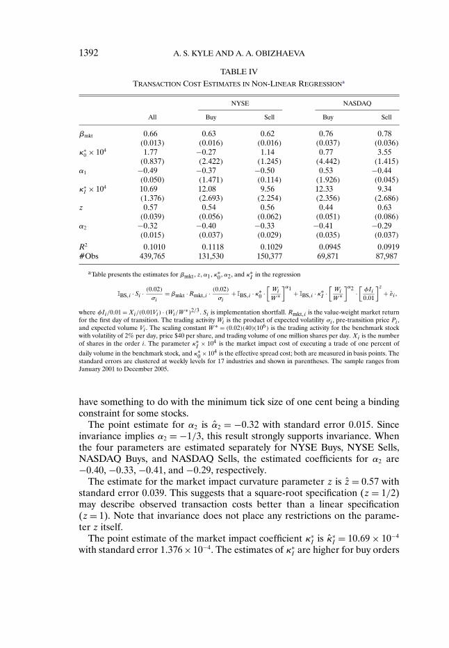
1392 A. S. KYLE AND A. A. OBIZHAEVA
TABLE IV
TRANSACTION COST ESTIMATES IN NON-LINEAR REGRESSIONa
NYSE NASDAQ
All Buy Sell Buy Sell
βmkt 0�66 0�63 0�62 0�76 0�78(0�013) (0�016) (0�016) (0�037) (0�036)
κ∗0 × 104 1�77 −0�27 1�14 0�77 3�55
(0�837) (2�422) (1�245) (4�442) (1�415)α1 −0�49 −0�37 −0�50 0�53 −0�44
(0�050) (1�471) (0�114) (1�926) (0�045)κ∗I × 104 10�69 12�08 9�56 12�33 9�34
(1�376) (2�693) (2�254) (2�356) (2�686)z 0�57 0�54 0�56 0�44 0�63
(0�039) (0�056) (0�062) (0�051) (0�086)α2 −0�32 −0�40 −0�33 −0�41 −0�29
(0�015) (0�037) (0�029) (0�035) (0�037)
R2 0�1010 0�1118 0�1029 0�0945 0�0919#Obs 439,765 131,530 150,377 69,871 87,987
aTable presents the estimates for βmkt� z�α1�κ∗0�α2, and κ∗
I in the regression
IBS�i · Si ·(0�02)σi
= βmkt ·Rmkt�i ·(0�02)σi
+ IBS�i · κ∗0 ·
[WiW ∗
]α1 + IBS�i · κ∗I ·
[WiW ∗
]α2 ·[φIi0�01
]z+ εi�
where φIi/0�01 =Xi/(0�01Vi) · (Wi/W ∗)2/3. Si is implementation shortfall. Rmkt�i is the value-weight market returnfor the first day of transition. The trading activity Wi is the product of expected volatility σi , pre-transition price Pi ,and expected volume Vi . The scaling constant W ∗ = (0�02)(40)(106) is the trading activity for the benchmark stockwith volatility of 2% per day, price $40 per share, and trading volume of one million shares per day. Xi is the numberof shares in the order i. The parameter κ∗
I × 104 is the market impact cost of executing a trade of one percent of
daily volume in the benchmark stock, and κ∗0 × 104 is the effective spread cost; both are measured in basis points. The
standard errors are clustered at weekly levels for 17 industries and shown in parentheses. The sample ranges fromJanuary 2001 to December 2005.
have something to do with the minimum tick size of one cent being a bindingconstraint for some stocks.
The point estimate for α2 is α2 = −0�32 with standard error 0�015. Sinceinvariance implies α2 = −1/3, this result strongly supports invariance. Whenthe four parameters are estimated separately for NYSE Buys, NYSE Sells,NASDAQ Buys, and NASDAQ Sells, the estimated coefficients for α2 are−0�40, −0�33, −0�41, and −0�29, respectively.
The estimate for the market impact curvature parameter z is z = 0�57 withstandard error 0�039. This suggests that a square-root specification (z = 1/2)may describe observed transaction costs better than a linear specification(z = 1). Note that invariance does not place any restrictions on the parame-ter z itself.
The point estimate of the market impact coefficient κ∗I is κ∗
I = 10�69 × 10−4
with standard error 1�376 × 10−4. The estimates of κ∗I are higher for buy orders

MARKET MICROSTRUCTURE INVARIANCE 1393
than for sell orders (12�08 × 10−4 versus 9�56 × 10−4 for NYSE; 12�33 × 10−4
versus 9�34 × 10−4 for NASDAQ).Note that the point estimate of the market impact coefficient κ∗
I is differentfrom zero with much greater statistical significance than the bid-ask spreadcoefficient κ∗
0; this is consistent with the interpretation that market impact costsare of considerably greater economic importance than bid-ask spread costs.
Results for the five-parameter linear specification, regression equation (31)with the parameter restriction z = 1 (linear impact), are reported in Table A.IIIin the Supplemental Material. The estimate of the bid-ask spread cost κ∗
0 is6�28 × 10−4 with standard error 0�890 × 10−4, and the estimate of the exponentα1 is α1 = −0�39 with standard error 0�020. The estimate of the market impactcost κ∗
I is 2�73 × 10−4 with standard error 0�252. The estimate of the exponentα2 is α2 = −0�31 with standard error of 0�028; thus, under the restriction oflinear price impact (z = 1), the additional restriction imposed by invariance(α2 = 1/3) is not statistically rejected.
Model Calibration
Next, we calibrate transaction-cost models under the assumption of invari-ance and the assumption of either linear or square-root specification for thecost function.
Table V presents estimates for the three parameters βmkt, κ∗0, and κ∗
I in equa-tion (31), imposing the invariance restrictions α1 = α2 = −1/3 and also impos-ing either a linear transaction-cost model z = 1 or a square-root model z = 1/2.
In the linear specification with z = 1, the point estimate for market impactcost κ∗
I is equal to 2�50 × 10−4, and the point estimate for bid-ask spread costκ∗
0 is equal to 8�21 × 10−4.In the square-root specification with z = 1/2, the point estimate for market
impact cost κ∗I is equal to 12�08 × 10−4, and the point estimate for half bid-ask
spread κ∗0 is equal to 2�08 × 10−4.
For the benchmark stock, these estimates imply that the total cost of a hypo-thetical trade of one percent of daily volume incurs a cost of about 10�71 basispoints in the linear model and 14�16 basis points in the square-root model.
The benchmark stock would belong to volume group 7, and the correspond-ing average quoted spread in Table I for that group is 12�04 basis points. Theimplied spread estimate of about 16�42 basis points for the linear model is closeto the quoted spread; the implied spread estimate of 4�16 basis points for thesquare-root model may be biased downward due to collinearity between theconstant term and the square-root term in the regression in the region close tozero.
Economic Interpretation
We examine the economic significance of our results by comparing the R2 ofdifferent specifications for transaction-cost models.
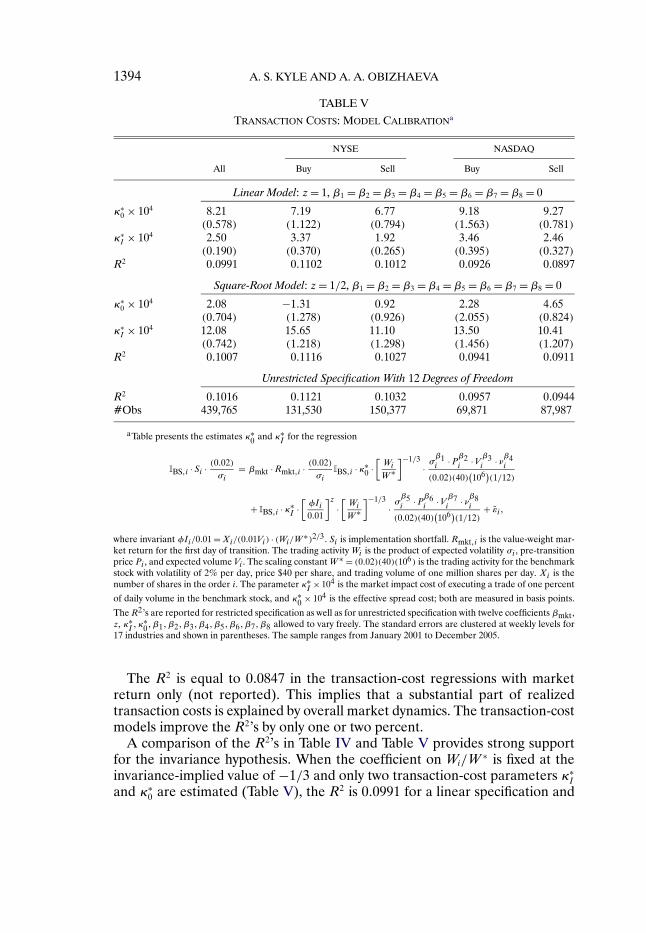
1394 A. S. KYLE AND A. A. OBIZHAEVA
TABLE V
TRANSACTION COSTS: MODEL CALIBRATIONa
NYSE NASDAQ
All Buy Sell Buy Sell
Linear Model: z = 1, β1 = β2 =β3 = β4 = β5 = β6 = β7 = β8 = 0
κ∗0 × 104 8�21 7�19 6�77 9�18 9�27
(0�578) (1�122) (0�794) (1�563) (0�781)κ∗I × 104 2�50 3�37 1�92 3�46 2�46
(0�190) (0�370) (0�265) (0�395) (0�327)R2 0�0991 0�1102 0�1012 0�0926 0�0897
Square-Root Model: z = 1/2, β1 = β2 = β3 = β4 = β5 =β6 = β7 = β8 = 0
κ∗0 × 104 2�08 −1�31 0�92 2�28 4�65
(0�704) (1�278) (0�926) (2�055) (0�824)κ∗I × 104 12�08 15�65 11�10 13�50 10�41
(0�742) (1�218) (1�298) (1�456) (1�207)R2 0�1007 0�1116 0�1027 0�0941 0�0911
Unrestricted Specification With 12 Degrees of Freedom
R2 0�1016 0�1121 0�1032 0�0957 0�0944#Obs 439,765 131,530 150,377 69,871 87,987
aTable presents the estimates κ∗0 and κ∗
I for the regression
IBS�i · Si ·(0�02)σi
= βmkt ·Rmkt�i ·(0�02)σi
IBS�i · κ∗0 ·
[WiW ∗
]−1/3· σ
β1i · Pβ2
i · V β3i · νβ4
i
(0�02)(40)(106)
(1/12)
+ IBS�i · κ∗I ·
[φIi0�01
]z·[WiW ∗
]−1/3· σ
β5i · Pβ6
i · V β7i · νβ8
i
(0�02)(40)(106)
(1/12)+ εi�
where invariant φIi/0�01 =Xi/(0�01Vi) · (Wi/W ∗)2/3. Si is implementation shortfall. Rmkt�i is the value-weight mar-ket return for the first day of transition. The trading activity Wi is the product of expected volatility σi , pre-transitionprice Pi , and expected volume Vi . The scaling constant W ∗ = (0�02)(40)(106) is the trading activity for the benchmarkstock with volatility of 2% per day, price $40 per share, and trading volume of one million shares per day. Xi is thenumber of shares in the order i. The parameter κ∗
I × 104 is the market impact cost of executing a trade of one percent
of daily volume in the benchmark stock, and κ∗0 × 104 is the effective spread cost; both are measured in basis points.
The R2’s are reported for restricted specification as well as for unrestricted specification with twelve coefficients βmkt,z, κ∗
I �κ∗0�β1�β2�β3�β4�β5�β6�β7�β8 allowed to vary freely. The standard errors are clustered at weekly levels for
17 industries and shown in parentheses. The sample ranges from January 2001 to December 2005.
The R2 is equal to 0�0847 in the transaction-cost regressions with marketreturn only (not reported). This implies that a substantial part of realizedtransaction costs is explained by overall market dynamics. The transaction-costmodels improve the R2’s by only one or two percent.
A comparison of the R2’s in Table IV and Table V provides strong supportfor the invariance hypothesis. When the coefficient on Wi/W
∗ is fixed at theinvariance-implied value of −1/3 and only two transaction-cost parameters κ∗
I
and κ∗0 are estimated (Table V), the R2 is 0�0991 for a linear specification and
MARKET MICROSTRUCTURE INVARIANCE 1395
0�1007 for a square-root specification. The square-root specification performsbetter than the linear specification. Compared with the square-root specifica-tion, adding the three additional parameters α1, α2, and z modestly increasesthe R2 from 0�1007 to 0�1010 (Table V). The modest increase strongly supportsthe economic importance of invariance.
We also consider a more general specification with eleven estimated coeffi-cients. The exponents on the three components of trading activityWi (volatilityσi, price Pi, volume Vi) as well as the exponent on the monthly turnover νi areallowed to vary freely. The estimated regression equation is
IBS�i · Si · (0�02)σi
(32)
= βmkt ·Rmkt�i · (0�02)σi
IBS�i · κ∗0 ·
[Wi
W ∗
]−1/3
· σβ1i · Pβ2
i · V β3i · νβ4
i
(0�02)(40)(106
)(1/12)
+ IBS�i · κ∗I ·
[φIi
0�01
]z·[Wi
W ∗
]−1/3
· σβ5i · Pβ6
i · V β7i · νβ8
i
(0�02)(40)(106
)(1/12)
+ εi�
Because the exponents on the W -terms are set to be −1/3, the invariance hy-potheses predict β1 = β2 = β3 = β4 = β5 = β6 = β7 = β8 = 0.
Table V shows that despite increasing the number of estimated parametersfrom four to eleven, the R2 in the aggregate regression increases from 0�1010to only 0�1016. The estimates of β1, β2, β3, β4, β5, β6, β7, and β8 are shown inTable A.IV in the Supplemental Material. The estimates of β1, β2, β3, β4 areoften statistically significant, but these explanatory variables are multiplied bystatistically insignificant coefficient κ∗
0. Almost all estimates of β5, β6, β7, andβ8 are statistically insignificant, both for the pooled sample as well as the foursubsamples.
In all three specifications, separate regressions for NYSE Buys, NYSE Sells,NASDAQ Buys, and NASDAQ Sells suggest that price-impact costs are higherfor buy orders than for sell orders. This is consistent with the hypothesis, dis-cussed by Obizhaeva (2009), that the market believes that buy orders—in par-ticular, buy orders in portfolio transitions—contain more information than sellorders.
OLS Estimates for Quoted Spread
Finally, we present results of statistical tests based on the data on quotedbid-ask spread for portfolio transition orders.
Since invariance implies that bid-ask spread costs are proportional to σi ·W −1/3i , intuition suggests that quoted spreads may also have this invariant prop-
erty. As a supplement to our empirical results on transaction costs, we test thisprediction using data on quoted spreads, supplied in the portfolio transitiondata as pre-trade information for each transition order.

1396 A. S. KYLE AND A. A. OBIZHAEVA
Let si denote the dollar quoted spread for order i. Using equations (1)and (2), we can write equation (19) as the log-linear OLS regression
ln[
si
Pi · σi]
= ln s+ α3 · ln[Wi
W ∗
]+ εi�(33)
where invariance implies α3 = −1/3. The constant term ln[s] := ln[s∗/(40 · 0�02)] + 2/3 · ln[ψ/ψ∗] − 1/3 · ln[ζ∗/ζ] quantifies the dollar spread s∗for the benchmark stock as a fraction of dollar volatility P∗ · σ∗, under theidentifying assumptions ζ = ζ∗ and ψ=ψ∗.
Table VI presents the regression results. The point estimate α3 = −0�35 hasstandard error 0�003. For subsamples of NYSE Buys, NYSE Sells, NASDAQBuys, and NASDAQ Sells, the estimates are −0�31, −0�32, −0�40, and −0�39,respectively. Although the hypothesis α3 = −1/3 is usually rejected statistically,the estimates are economically close to the value of −1/3 predicted by invari-ance. The point estimate of ln[s] is equal to −3�07, implying a quoted spread ofexp(−3�07) · 0�02 ≈ 9 × 10⁻⁴ for the benchmark stock. This number is similarto the median spread of 8�12 basis points for volume group 7 in Table I.
It can be shown that an implicit spread proportional to σi · W −1/3i , as implied
by invariance, provides a better proxy for the actually incurred spread coststhan the quoted spread itself. When regression equation (31) is estimated with
TABLE VI
OLS ESTIMATES OF LOG OF QUOTED SPREADa
NYSE NASDAQ
All Buy Sell Buy Sell
ln[s] −3�07 −3�09 −3�08 −3�04 −3�04(0�008) (0�008) (0�008) (0�013) (0�012)
α3 −0�35 −0�31 −0�32 −0�40 −0�39(0�003) (0�003) (0�003) (0�004) (0�004)
R2 0�4744 0�3545 0�3964 0�5516 0�5721eln[s] · 0�02 × 104 9�28 9�10 9�19 9�57 9�57#Obs 434,920 130,700 149,197 68,833 86,190
aTable presents the estimates ln[s] and α3 for the regression
ln[
siPi · σi
]= ln[s] + α3 · ln
[WiW ∗
]+ εi�
Each observation corresponds to order i. The left side variable is the logarithm of the quoted bid-ask spread si/Pias a fraction of expected returns volatility σi . The trading activity Wi is the product of expected daily volatility σi ,pre-transition price Pi , and expected daily volume Vi , measured as the last month’s average daily volume. The scalingconstant W ∗ = (0�02)(40)(106) corresponds to the trading activity for the benchmark stock with volatility of 2% perday, price $40 per share, and trading volume of one million shares per day. The quantity exp(ln[s]) ·0�02×104 measuresthe median percentage spread for the benchmark stock in basis points. The standard errors are clustered at weeklylevels for 17 industries and shown in parentheses. The sample ranges from January 2001 to December 2005.

MARKET MICROSTRUCTURE INVARIANCE 1397
linear impact z = 1, using only the 436,649 observations for which quoted bid-ask spread data are supplied, we find the R2 is equal to 0�0992. Now replacethe invariance-implied spread cost proportional to σi · W −1/3
i with the quotedhalf spread 1/2 · si/Pi in equation (17). The estimated equation is
IBS�i · Si · (0�02)σi
= βmkt ·Rmkt�i · (0�02)σi
+ IBS�i ·βS · 12
· siPi
· (0�02)σi
(34)
+ IBS�i · κI ·[φIi
0�01
]·[Wi
W ∗
]α2
+ εi�
We find that the R2 drops from 0�0992 to 0�0976 (Table A.V in the Supplemen-tal Material). The point estimate of the coefficient on the quoted half-spreadcoefficient is βS = 0�71. The estimates are equal to 0�61, 0�74, 0�61, and 0�75,when estimated for NYSE Buys, NYSE Sells, NASDAQ Buys, and NASDAQSells, respectively.
One interpretation of the estimate of 0�71 is that transition managers incuras a transaction cost only 71% of the quoted half-spread. The values are con-sistent with the intuition in Goettler, Parlour, and Rajan (2005) that endoge-nously optimizing traders capture a fraction of the bid-ask spread by mixingbetween market orders and limit orders. Another interpretation is that noisein the quoted spread biases the coefficient towards zero and reduces the ex-planatory power of the regression.
Bouchaud, Farmer, and Lillo (2009) and Dufour and Engle (2000) reportedthat the quoted bid-ask spread is proportional to the standard deviation of per-centage returns between trades; this result is implied by microstructure invari-ance under the assumption that the rate at which trades occur is proportionalto the rate at which bets arrive. Stoll (1978a) proposed a theory that the per-centage dealer bid-ask spread in NASDAQ stocks is proportional to variablesincluding the dealer holding period and the returns variance of the stock; thiscaptures the spirit of invariance if the dealer holding period is proportional tothe rate at which bets arrive. Stoll (1978b) also tested this theory using data ondealer spreads for NASDAQ stocks, and his estimates are consistent with ourfindings as well.13
13Stoll (1978b) reported an R2 of approximately 0�82 in an OLS regression of percentage bid-ask spread on the logs of various variables including dollar volume, stock price, returns variance,turnover, and number of dealers. Using the standard deviations and correlation matrix for thevariables (p. 1165), it can be shown that imposing coefficients of −1/3 on dollar volume and+1/3 on returns variance (to mimic the definition of 1/Li), while imposing coefficients of zeroon all other explanatory variables except a constant term, results in an R2 equal to 0�66. Thisresult is similar to our results in Table VI.

1398 A. S. KYLE AND A. A. OBIZHAEVA
Discussion
Figure 5 plots the estimated coefficients for the 100 dummy variables, alongwith their 95% confidence intervals, estimated from the dummy variable re-gression equation (30) by pooling the data across all 10 volume groups. Thelinear and square-root cost functions with parameters calibrated in Table V aresuperimposed. The linear specification is 2�50 × 10−4 · φI/0�01 + 8�21 × 10−4
(solid black line), and the square-root specification is 12�07×10−4 ·√φI/0�01+2�08 × 10−4 (solid gray line). Both specifications result in estimates economi-cally close to each other.
Consistent with the higher reported R2 for the square-root model than thelinear model in Table V, the square-root specification fits the data slightly bet-ter than the linear specification, particularly for large orders in the order sizebins from 90th to 99th percentiles. Consistent with our results, most studiesfind that total price impact is best described by a concave function.14 For ex-
FIGURE 5.—Transaction-cost functions. Figure shows estimates of transaction-cost func-tions based on entire sample. On the horizonal axis, there are 100 equally spaced binsbased on re-scaled order sizes, φI = X/V · (Wi/W
∗)2/3. The plot contains 100 estimatesf ∗(k�h)/L∗�h= 1� � � � �100 from the regression
IBS�i · Si · (0�02)σi
= βmkt ·Rmkt�i · (0�02)σi
+ IBS�i ·[Wi
W ∗
]−1/3
·100∑h=1
D∗i (k�h) · f ∗(k�h)/L∗ + εi�
Xi is an order size in shares, Vi is the average daily volume in shares, and Wi is the mea-sure of trading activity. The vertical axis presents estimated transaction-cost invariant f ∗(·)/Liin basis points. The 95th percent confidence intervals are superimposed (dotted lines). A lin-ear function is 2�50 × 10−4 · φI/0�01 + 8�21 × 10−4 (black solid line). A square-root function is12�07 × 10−4 · √φI/0�01 + 2�08 × 10−4 (gray solid line). The sample ranges from January 2001 toDecember 2005.
14Since we plot the log of order size on the horizontal axis but do not take the log of the trans-action cost on the vertical axis (to make standard errors have similar magnitudes for different
MARKET MICROSTRUCTURE INVARIANCE 1399
ample, Almgren et al. (2005) obtained an estimate z = 0�60 for their sam-ple of almost 30,000 U.S. stock orders executed by Citigroup between 2001and 2003; this is comparable to our estimate of z = 0�56 when the constraintα1 = α2 = −1/3 is imposed in regression equation (31). To differentiate tempo-rary impact from permanent impact of earlier executed trades, Almgren et al.(2005) assumed a particular execution algorithm with a constant rate of trad-ing. We do not quantify these cost components separately but rather focus ontotal costs.
Intuition might suggest that for gigantic orders, the square-root model wouldpredict dramatically lower transaction costs than the linear model, making iteasy to distinguish the predictions of one model from the other. As the super-imposed estimated linear and square-root cost functions for the ten plots inFigure 4 make clear, both specifications estimate similar transaction costs forthe bin representing the largest 1% of orders (because the graphs of the lin-ear and square-root functions in Figure 5 cross near the bin representing thelargest 1% of orders). Furthermore, the transaction-cost dummy variable forthe largest 1% of orders fits both the linear and square-root models well. Forthe largest 1% of orders in the highest-volume group in Figure 4, the estimateddummy variable fits the higher cost estimates of the linear model better thanthe square-root model.
We have developed notation which allows the possibility that the parametersζjt , ψjt , and δjt vary across stocks j and time t. Although our parameter esti-mates are economically close to the ones predicted by invariance, it is possiblethat ζjt , ψjt , and δjt do vary across j and t enough to statistically reject theinvariance hypotheses in some cases. The notation we have developed can beused to investigate this possibility in future research.
6. IMPLICATIONS
The invariance relationships (7), (8), and (16) are like a structural modelwhich describes the implications of market microstructure for bet sizes andtransaction costs. The model is fully specified by constants describing the mo-ments of I and the shape of the un-modeled function CB(·), which determinesthe constant CB. These constants can be inferred from the estimates in Sec-tion 4 and Section 5, but their economic interpretation depends on assump-tions about the volume multiplier ζ, the volatility multiplier ψ, and the defla-tor δ.
Our empirical tests provide not only evidence in favor of the invariance hy-potheses but also inputs for calibration. Our empirical results can be summa-rized as follows. The distribution of portfolio transition orders |X|—expressed
observations), both the linear model and the concave square-root model show up as exponentialfunctions; the graph of the linear model is more convex than the graph of the square-root model.

1400 A. S. KYLE AND A. A. OBIZHAEVA
as a fraction of volume—is approximately a log-normal. It is therefore fully de-scribed by two parameters, the log-mean for the benchmark stock estimated tobe −5�71 and the log-variance estimated to be 2�53 (Table III). The followingformula shows how these estimates can be extrapolated to stocks with otherlevels of trading activity Wjt = σjt · Pjt · Vjt and volume Vjt :
ln[ |Xjt |Vjt
]≈ −5�71 − 2
3· ln
[Wjt
(0�02)(40)(106
)]
+ √2�53 · Z�(35)
Z ∼N(0�1)�
γjt = 85 ·[
Wjt
(0�02)(40)(106
)]2/3
�(36)
The last equation for the number of bets γjt follows directly from equation (35)under the assumption that the volume multiplier ζ = 2 and the portfolio tran-sition size multiplier δ= 1. These two equations fully describe the order-flowprocess.
Our empirical results also suggest that transaction-cost functions can be de-scribed by either a linear model or a square-root model. Since both modelsalso have a constant bid-ask spread term, each model is described by two pa-rameters. For an order of 1% of average daily volume in the benchmark stock,the estimates imply market impact costs of κI = 2�50 × 10−4 and spread costsof κ0 = 8�21 × 10−4 for the linear model as well as market impact costs ofκI = 12�08 × 10−4 and spread costs of κ0 = 2�08 × 10−4 for the square-rootmodel (Table V). The following formulas show how these estimates can be ex-trapolated to execution costs of an order of X shares for stocks with otherlevels of trading activity Wjt , volume Vjt , and volatility σjt :
Cjt(X)= σjt
0�02
(8�21104 ·
[Wjt
(0�02)(40)(106
)]−1/3
(37)
+ 2�50104 ·
[Wjt
(0�02)(40)(106
)]1/3
X
(0�01)Vjt
)�
Cjt(X)= σjt
0�02
(2�08104 ·
[Wjt
(0�02)(40)(106
)]−1/3
(38)
+ 12�08104 ·
[X
(0�01)Vjt
]1/2)�
These two equations fully describe the transaction-cost models.To summarize, formulas (35), (36), (37), and (38) provide a simple way to
calculate the number of bets, different percentiles of bet sizes, and transaction
MARKET MICROSTRUCTURE INVARIANCE 1401
costs. The only stock-specific inputs required are expected dollar volume andvolatility.15
Our results can also be used to calibrate the distribution of I and the invari-ant cost functionCB(·), which further implies specific quantitative relationshipsconcerning various market microstructure variables such as the number of betsper day, bet sizes, bid-ask spread, and market impact as functions of easily ob-servable trading activity and its components. These implications ultimately de-pend on values assigned to the volatility multiplier ψ, the volume multiplier ζ,and the deflator δ.
In a more complicated exercise left for future research, this handful of pa-rameters would make it possible to triangulate the value of parameters mea-suring the fraction of trading volume due to long-term investors rather thanintermediaries 1/ζ, the fraction of returns volatility generated by bets ψ, andthe ratio of the size of bets to the size of portfolio transition orders δ. In thefuture, careful thinking about calibration of the invariants and estimation ofmultipliers will be necessary to sharpen predictions based on invariance hy-potheses.
7. CONCLUSION
We have shown that the predictions based on market microstructure invari-ance are economically consistent with estimates from portfolio transitions datafor U.S. equities. We conjecture that predictions based on invariance may holdin other data as well, such as quotes and trades in the TAQ data set, insti-tutional holdings recorded in 13-F filings, institutional trades reported in theAncerno data set, and other data sets. For example, we conjecture that data onnews articles can help to show that information flows take place in the samebusiness time as trading.
We conjecture that predictions of market microstructure invariance maygeneralize to other markets such as bond markets, currency markets, and fu-tures markets, as well as to other countries. Whether market microstructureinvariance applies to other markets poses an interesting set of issues for futureresearch.
We do not expect invariance to hold perfectly across different markets anddifferent time periods. Differences in trading institutions across markets mightmake the volume multiplier and the volatility multiplier vary across markets.We expect transaction costs, particularly bid-ask spread costs (but perhaps not
15If one attempts to apply these formulas to assets or time periods where the values for the vol-ume multiplier ζ and the volatility multiplier ψ may be different from the ones relevant for oursample of portfolio transitions, then a simple adjustment to the formulas must be implemented.First, one needs to deflate trading volume and trading volatility in those formulas by appropriatemultipliers in order to write those formulas in terms of bet volume and bet volatility for obser-vations in portfolio transitions data. Second, one needs to plug into the modified formulas betvolume and bet volatility appropriate for the market for which calculations are made.
1402 A. S. KYLE AND A. A. OBIZHAEVA
market impact costs), to be influenced by numerous institutional features, suchas government regulation (e.g., short sale restrictions, customer order handlingrules), transaction taxes, competitiveness of market making institutions, effi-ciency of trading platforms, market fragmentation, technological change, andtick size. For example, if minimum tick size rules affect bid-ask spread costs,we believe that market microstructure invariance can be used as a benchmarkagainst which the effect of tick size on bid-ask spread costs can be evaluated.
To conclude, market microstructure invariance implies simple scaling lawswhich lead to sharp statistical hypotheses about bet size and transaction costs.Its implications explain an economically significant portion of the variation inportfolio transition order size and transaction costs when the scaling laws areimposed on the data. The scaling laws enable us to derive simple operationalformulas describing order-size distributions and transaction costs; thus, theyprovide simple benchmarks from which past research can be evaluated andopen up new lines of research in market microstructure.
REFERENCES
AITCHISON, J., AND J. A. C. BROWN (1957): The Lognormal Distribution With Special Referenceto Its Uses in Economics. Cambridge: Cambridge University Press. [1383]
ALLAIS, M. (1956): “Explication des Cycles Economiques Par Un Modele Non Linéaire a Régu-lation Retardée,” Metroeconomica, 8 (1), 4–83. [1348]
(1966): “A Restatement of the Quantity Theory of Money,” American Economic Review,56 (5), 1123–1157. [1348]
ALMGREN, R., C. THUM, E. HAUPTMANN, AND H. LI (2005): “Direct Estimation of Equity Mar-ket Impact,” Risk, 18 (7), 58–62. [1358,1399]
AMIHUD, Y. (2002): “Illiquidity and Stock Returns: Cross-Section and Time-Series Effects,” Jour-nal of Financial Markets, 5, 31–56. [1357,1366]
ANÉ, T., AND H. GEMAN (2000): “Order Flow, Transaction Clock, and Normality of Asset Re-turns,” Journal of Finance, 55 (5), 2259–2284. [1348]
BACK, K., AND S. BARUCH (2004): “Information in Securities Markets: Kyle Meets Glosten andMilgrom,” Econometrica, 72, 433–465. [1363,1364]
BOUCHAUD, J.-P., D. J. FARMER, AND F. LILLO (2009): “How Markets Slowly Digest Changes inSupply and Demand,” in Handbook of Financial Markets: Dynamics and Evolution. Amsterdam:North-Holland, 47–160. [1383,1397]
BREEN, W., L. S. HODRICK, AND R. A. KORAJCZYK (2002): “Predicting Equity Liquidity,” Man-agement Science, 48, 470–483. [1363]
BRENNAN, M., AND A. SUBRAHMANYAM (1998): “The Determinants of Average Trade Size,”Journal of Business, 71 (1), 1–25. [1363]
CAMPBELL, J. Y., AND A. S. KYLE (1993): “Smart Money, Noise Trading, and Stock Price Behav-ior,” Review of Economic Studies, 60, 1–34. [1363]
CLARK, P. K. (1973): “A Subordinated Stochastic Process Model With Finite Variance for Specu-lative Prices,” Econometrica, 41, 135–155. [1348,1382,1383]
DERMAN, E. (2002): “The Perception of Time, Risk and Return During Periods of Speculation,”Quantitative Finance, 2, 282–296. [1348,1358]
DUFOUR, A., AND R. F. ENGLE (2000): “Time and the Price Impact of a Trade,” Journal of Fi-nance, 55 (6), 2467–2598. [1348,1397]
GABAIX, X., P. GOPIKRISHNAN, V. PLEROU, AND E. H. STANLEY (2006): “Institutional Investorsand Stock Market Volatility,” Quarterly Journal of Economics, 121, 461–504. [1358,1359,1382]

MARKET MICROSTRUCTURE INVARIANCE 1403
GLOSTEN, L. R., AND P. R. MILGROM (1985): “Bid, Ask and Transaction Prices in a SpecialistMarket With Heterogeneously Informed Traders,” Journal of Financial Economics, 14, 71–100.[1363,1364]
GOETTLER, R. L., C. A. PARLOUR, AND U. RAJAN (2005): “Equilibrium in a Dynamic LimitOrder Market,” Journal of Finance, 60 (5), 2149–2192. [1397]
GOPIKRISHNAN, P., M. MEYER, L. A. AMARAL, AND E. H. STANLEY (1998): “Inverse Cubic Lawfor the Distribution of Stock Price Variations,” European Physical Journal, 3, 139–140. [1382]
GRINOLD, R. C., AND R. N. KAHN (1999): Active Portfolio Management: A Quantitative Approachfor Providing Superior Returns and Controlling Risk (Second Ed.). New York: McGraw-Hill.[1359]
GROSSMAN, S. J., AND M. H. MILLER (1988): “Liquidity and Market Structure,” Journal of Fi-nance, 43 (3), 617–633. [1363]
GROSSMAN, S. J., AND J. E. STIGLITZ (1980): “On the Impossibility of Informationally EfficientMarkets,” American Economic Review, 70 (3), 393–408. [1363]
HASBROUCK, J. (1999): “Trading Fast and Slow: Security Market Events in Real Time,” NYUWorking Paper FIN-99-012, SSRN-id1296401, available at http://archive.nyu.edu/bitstream/2451/26851/2/wpa99012.pdf. [1348]
(2007): Empirical Market Microstructure: The Institutions, Economics, and Econometricsof Securities Trading. New York: Oxford University Press. [1363]
HOLDEN, C. W., S. JACOBSEN, AND A. SUBRAHMANYAM (2014): “The Empirical Analysis of Liq-uidity,” Foundations and Trends in Finance 8 (4), 263–365. [1363]
KOLMOGOROV, A. N. (1941a): “The Local Structure of Turbulence in Incompressible Vis-cous Fluids at Very Large Reynolds Numbers,” Doklady Akademii Nauk SSSR, 30, 301–305.Reprinted in Procedings of the Royal Society London A, 434, 1991, 9–13. [1362]
(1941b): “On the Log-Normal Distribution of Particle Sizes During Break-up Process,”Doklady Akademii Nauk SSSR, 31 (2), 99–101. [1383]
KYLE, A. S. (1985): “Continuous Auctions and Insider Trading,” Econometrica, 53 (6), 1315–1335.[1346,1358,1363-1365]
KYLE, A. S., AND A. A. OBIZHAEVA (2016a): “Large Bets and Stock Market Crashes,” WorkingPaper, available at http://dx.doi.org/10.2139/ssrn.2023776. [1347,1382]
(2016b): “Market Microstructure Invariance: A Dynamic Equilibrium Model,” WorkingPaper, University of Maryland, available at http://papers.ssrn.com/sol3/papers.cfm?abstract_id=2749531. [1345,1348,1362]
(2016c): “Supplement to ‘Market Microstructure Invariance: Empirical Hypotheses’,”Econometrica Supplemental Material, 84, http://dx.doi.org/10.3982/ECTA10486. [1367]
LEE, C., AND M. READY (1991): “Inferring Trade Direction From Intraday Data,” Journal ofFinance, 46, 733–746. [1363]
LOEB, T. (1983): “Trading Cost: The Critical Link Between Investment Information and Results,”Financial Analysts Journal, 39, 39–44. [1359]
MANDELBROT, B., AND H. M. TAYLOR (1967): “On the Distribution of Stock Price Differences,”Operations Research, 15 (6), 1057–1062. [1348,1382,1383]
MODIGLIANI, F., AND M. H. MILLER (1958): “The Cost of Capital, Corporation Finance and theTheory of Investment,” American Economic Review, 48, 261–297. [1348]
OBIZHAEVA, A. (2009): “Portfolio Transitions and Price Dynamics,” Working Paper, NewEconomic School, available at http://papers.ssrn.com/sol3/papers.cfm?abstract_id=2591294.[1395]
(2012): “Liquidity Estimates and Selection Bias,” Working Paper, New EconomicSchool, available at http://papers.ssrn.com/sol3/papers.cfm?abstract_id=1178722. [1384]
PEROLD, A. (1988): “The Implementation Shortfall: Paper vs. Reality,” Journal of Portfolio Man-agement, 14 (3), 4–9. [1383]
PLEROU, V., P. GOPIKRISHNAN, L. A. AMARAL, X. GABAIX, AND E. H. STANLEY (2000): “Eco-nomic Fluctuations and Anomalous Diffusion,” Physical Review E, 62, 3023–3026. [1348,1382]

1404 A. S. KYLE AND A. A. OBIZHAEVA
SCHWARZKOPF, Y., AND D. J. FARMER (2010): “Empirical Study of the Tails of Mutual FundSize,” Physical Review E, 81, 066113. [1383]
STAMBOUGH, R. F., AND L. PASTOR (2003): “Liquidity Risk and Expected Stock Returns,” Journalof Political Economy, 111, 642–685. [1357]
STOLL, H. R. (1978a): “The Supply of Dealer Services in Securities Markets,” Journal of Finance,33 (4), 1133–1151. [1397]
(1978b): “The Pricing of Security Dealer Services: An Empirical Study of NASDAQStocks,” Journal of Finance, 33 (4), 1153–1172. [1397]
TORRE, N. G. (1997): BARRA Market Impact Model Handbook. Berkeley: BARRA Inc. [1359]TREYNOR, J. (1995): “The Only Game in Town,” Financial Analysts Journal, 51 (1), 81–83.
Reprinted from Financial Analysts Journal, 22, 1971, 12–14. [1363]WANG, J. (1993): “A Model of Intertemporal Asset Prices Under Asymmetric Information,” Re-
view of Economic Studies, 60 (2), 249–282. [1363]
Robert H. Smith School of Business, University of Maryland, College Park,MD 20742, U.S.A.; [email protected]
andNew Economic School, 100A Novaya Street Skolkovo, Moscow 143025, Rus-
sia; [email protected].
Co-editor Lars Peter Hansen handled this manuscript.
Manuscript received December, 2011; final revision received February, 2016.
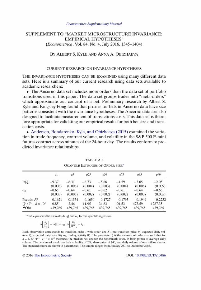
Econometrica Supplementary Material
SUPPLEMENT TO “MARKET MICROSTRUCTURE INVARIANCE:EMPIRICAL HYPOTHESES”
(Econometrica, Vol. 84, No. 4, July 2016, 1345–1404)
BY ALBERT S. KYLE AND ANNA A. OBIZHAEVA
CURRENT RESEARCH ON INVARIANCE HYPOTHESES
THE INVARIANCE HYPOTHESES CAN BE EXAMINED using many different datasets. Here is a summary of our current research using data sets available toacademic researchers:
• The Ancerno data set includes more orders than the data set of portfoliotransitions used in this paper. The data set groups trades into “meta-orders”which approximate our concept of a bet. Preliminary research by Albert S.Kyle and Kingsley Fong found that proxies for bets in Ancerno data have sizepatterns consistent with the invariance hypotheses. The Ancerno data are alsodesigned to facilitate measurement of transactions costs. This data set is there-fore appropriate for validating our empirical results for both bet size and trans-action costs.
• Andersen, Bondarenko, Kyle, and Obizhaeva (2015) examined the varia-tion in trade frequency, contract volume, and volatility in the S&P 500 E-minifutures contract across minutes of the 24-hour day. The results conform to pre-dicted invariance relationships.
TABLE A.I
QUANTILE ESTIMATES OF ORDER SIZEa
p1 p5 p25 p50 p75 p95 p99
ln[q] −9�37 −8�31 −6�73 −5�66 −4�59 −3�05 −2�05(0�008) (0�006) (0�004) (0�003) (0�004) (0�006) (0�009)
α0 −0�65 −0�64 −0�61 −0�62 −0�61 −0�64 −0�63(0�005) (0�003) (0�002) (0�002) (0�002) (0�003) (0�005)
Pseudo R2 0�1621 0�1534 0�1650 0�1727 0�1795 0�1949 0�2232Q∗/V ∗ · δ× 104 0�85 2�46 11�95 34�83 101�53 473�59 1287�35#Obs 439,765 439,765 439,765 439,765 439,765 439,765 439,765
aTable presents the estimates ln[q] and α0 for the quantile regression
ln[XiVi
]= ln[q] + α0 · ln
[WiW ∗
]+ εi�
Each observation corresponds to transition order i with order size Xi , pre-transition price Pi , expected daily vol-ume Vi , expected daily volatility σi , trading activity Wi . The parameter q is the measure of order size such that forδ = 1, Q∗/V ∗ · δ−1 × 10⁴ measures the median bet size for the benchmark stock, in basis points of average dailyvolume. The benchmark stock has daily volatility of 2%, share price of $40, and daily volume of one million shares.The standard errors are shown in parentheses. The sample ranges from January 2001 to December 2005.
© 2016 The Econometric Society DOI: 10.3982/ECTA10486
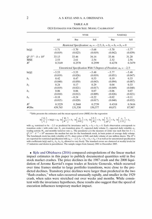
2 A. S. KYLE AND A. A. OBIZHAEVA
TABLE A.II
OLS ESTIMATES FOR ORDER SIZE: MODEL CALIBRATIONa
NYSE NASDAQ
All Buy Sell Buy Sell
Restricted Specification: α0 = −2/3, b1 = b2 = b3 = b4 = 0
ln[q] −5�71 −5�70 −5�68 −5�70 −5�77(0�019) (0�023) (0�019) (0�042) (0�039)
Q∗/V ∗ · δ× 104 33�13 33�46 34�14 33�46 31�20MSE 2�53 2�61 2�54 2�32 2�56R2 0�3149 0�2578 0�2599 0�4278 0�3479
Unrestricted Specification With 5 Degrees of Freedom: α0 = −2/3
ln[q] −5�53 −5�55 −5�48 −5�77 −5�48(0�019) (0�026) (0�019) (0�051) (0�047)
b1 0�42 0�47 0�53 0�19 0�33(0�040) (0�050) (0�043) (0�094) (0�087)
b2 0�24 0�17 0�29 0�04 0�33(0�019) (0�021) (0�017) (0�049) (0�040)
b3 0�06 0�06 0�07 −0�06 0�07(0�010) (0�012) (0�009) (0�026) (0�021)
b4 −0�18 −0�24 −0�22 −0�02 −0�11(0�015) (0�020) (0�017) (0�040) (0�032)
R2 0�3229 0�2668 0�2739 0�4318 0�3616#Obs 439,765 131,530 150,377 69,871 87,987
aTable presents the estimates and the mean squared error (MSE) for the regression
ln[XiVi
]= ln[q] + α0 · ln
[WiW ∗
]+ b1 · ln
[σi
0�02
]+ b2 · ln
[Pi40
]+ b3 · ln
[Vi
106
]+ b4 · ln
[νi
1/12
]+ εi�
with α0 restricted to be −2/3 as predicted by invariance and b1 = b2 = b3 = 0. Each observation corresponds totransition order i with order size Xi , pre-transition price Pi , expected daily volume Vi , expected daily volatility σi ,trading activity Wi , and monthly turnover rate νi . The parameter q is the measure of order size such that for δ = 1,Q∗/V ∗ · δ−1 × 10⁴ measures the median bet size for the benchmark stock, in basis points of average daily volume.The benchmark stock has daily volatility of 2%, share price of $40, and daily volume of one million shares. The R2’sare reported for restricted specification with α0 = −2/3, b1 = b2 = b3 = b4 = 0 as well as for unrestricted specificationwith coefficients ln[q] and b1� b2� b3� b4 allowed to vary freely. The standard errors are clustered at weekly levels for17 industries and shown in parentheses. The sample ranges from January 2001 to December 2005.
• Kyle and Obizhaeva (2016) compared extrapolations of the linear marketimpact estimates in this paper to publicly documented quantities sold in fivestock market crashes. The price declines in the 1987 crash and the 2008 liqui-dation of Jerome Kerviel’s rogue trades at Societe Generale, which occurredover time frames similar to large portfolio transitions, were close to the pre-dicted declines. Transitory price declines were larger than predicted in the two“flash crashes,” when sales occurred unusually rapidly, and smaller in the 1929crash, when sales were stretched out over weeks and months. While consis-tent with the invariance hypotheses, these results also suggest that the speed ofexecution influences temporary market impact.

MARKET MICROSTRUCTURE INVARIANCE 3
TABLE A.III
TRANSACTION-COST ESTIMATES IN REGRESSION WITH LINEAR IMPACTa
NYSE NASDAQ
All Buy Sell Buy Sell
βmkt 0�66 0�63 0�62 0�77 0�77(0�013) (0�016) (0�016) (0�037) (0�036)
κ∗0 × 104 6�28 6�51 5�43 5�94 6�54
(0�890) (1�600) (1�154) (2�147) (1�501)α1 −0�40 −0�36 −0�39 −0�44 −0�40
(0�020) (0�048) (0�029) (0�051) (0�031)κ∗I × 104 2�73 2�63 2�10 3�69 3�13
(0�252) (0�460) (0�346) (0�663) (0�765)α2 −0�31 −0�45 −0�31 −0�32 −0�28
(0�028) (0�038) (0�041) (0�056) (0�058)
R2 0�0993 0�1105 0�1014 0�0931 0�0901#Obs 439,765 131,530 150,377 69,871 87,987
aTable presents the estimates for βmkt�α1�κ∗0�α2, and κ∗
I in the regression
IBS�i · Si ·(0�02)σi
= βmkt ·Rmkt�i ·(0�02)σi
+ IBS�i · κ∗0 ·
[WiW ∗
]α1 + IBS�i · κ∗I ·
[WiW ∗
]α2 ·[φIi0�01
]z+ εi�
where z = 1 and φIi/0�01 = Xi/(0�01Vi) · (Wi/W ∗)2/3. Si is implementation shortfall. Rmkt�i is the value-weightmarket return for the first day of transition. The trading activity Wi is the product of expected volatility σi , pre-transition price Pi , and expected volume Vi . The scaling constant W ∗ = (0�02)(40)(106) is the trading activity for thebenchmark stock with volatility of 2% per day, price $40 per share, and trading volume of one million shares per day.Xi is the number of shares in the order i. The parameter κ∗
I × 104 is the market impact cost of executing a trade of
one percent of daily volume in the benchmark stock, and κ∗0 × 104 is the effective spread cost; both are measured in
basis points. The standard errors are clustered at weekly levels for 17 industries and shown in parentheses. The sampleranges from January 2001 to December 2005.
• Kyle, Obizhaeva, and Tuzun (2016) examined the hypothesis that the sizeof “prints” of stock market trades in Trade and Quotations (TAQ) data is pro-portional to the size of bets. This hypothesis holds up well during the 1990s,consistent with the interpretation that bets were negotiated and printed asblock trades. The hypothesis breaks down after 2001, when trade size collapsedtoward the round-lot minimum size of 100 shares for many trades. The changesafter 2001 may be the result of the reduction in the minimum tick size to onecent and the increased use of electronic order-shredding algorithms.
• Kyle, Obizhaeva, and Sinha (2012) examined whether the monthly fre-quency of Thomson Reuters news articles is proportional to the 2/3 power oftrading activity for individual stocks. The estimated exponent is close to thepredicted value of 2/3 prior to a strategic decision by Thomson Reuters to in-crease the number of news articles about less actively traded stocks, after whichthe coefficient changes in a manner consistent with their strategic decision.
Using a different proprietary data set, Bae, Kyle, Lee, and Obizhaeva (2014)examined the number of times individual trading accounts switch between buy-ing and selling individual stocks. Consistent with the predictions of invariance,

4 A. S. KYLE AND A. A. OBIZHAEVA
TABLE A.IV
TRANSACTION COSTS: MODEL CALIBRATIONa
NYSE NASDAQ
All Buy Sell Buy Sell
Linear Model: z = 1, β1 = β2 = β3 = β4 = β5 =β6 = β7 = β8 = 0
βmkt 0�6571 0�6308 0�6195 0�7693 0�7771(0�0135) (0�0159) (0�0158) (0�0371) (0�0365)
κ0 × 104 8�2134 7�1934 6�7698 9�1832 9�2658(0�5776) (1�1215) (0�7943) (1�5627) (0�7811)
κI × 104 2�5003 3�3663 1�9220 3�4614 2�4629
(0�1903) (0�3700) (0�2650) (0�3953) (0�3267)R2 0�0991 0�1102 0�1012 0�0926 0�0897
Square-Root Model: z = 1/2, β1 = β2 = β3 = β4 = β5 = β6 = β7 = β8 = 0
βmkt 0�6552 0�6285 0�6192 0�7598 0�7782(0�0134) (0�0158) (0�0159) (0�0365) (0�0364)
κ0 × 104 2�0763 −1�3091 0�9167 2�2844 4�6530(0�7035) (1�2779) (0�9264) (2�0554) (0�8244)
κI × 104 12�0787 15�6544 11�0986 13�5025 10�4063
(0�7416) (1�2177) (1�2979) (1�4564) (1�2069)R2 0�1007 0�1116 0�1027 0�0941 0�0911
(Continues)

MARKET MICROSTRUCTURE INVARIANCE 5
TABLE A.IV—Continued
NYSE NASDAQ
All Buy Sell Buy Sell
Unrestricted Specification With 12 Degrees of Freedom
βmkt 0�66 0�63 0�62 0�76 0�78(0�013) (0�016) (0�015) (0�036) (0�036)
κ∗0 × 104 0�94 −0�05 0�47 1�55 1�61
(0�675) (0�124) (0�556) (1�698) (1�148)β1 −0�43 −2�47 −1�08 −0�44 −0�46
(0�147) (0�890) (0�392) (0�489) (0�131)β2 0�17 2�87 0�23 0�20 0�11
(0�072) (1�230) (0�231) (0�127) (0�109)β3 −0�56 1�85 −0�47 −0�47 −0�49
(0�159) (0�754) (0�296) (0�238) (0�155)β4 0�62 0�13 0�49 0�49 0�58
(0�173) (0�620) (0�490) (0�313) (0�175)κ∗I × 104 9�36 11�61 10�93 8�88 5�00
(1�307) (2�471) (1�804) (3�340) (2�033)z 0�58 0�54 0�52 0�58 0�63
(0�041) (0�039) (0�042) (0�094) (0�083)β5 0�02 −0�11 0�36 −0�17 −0�23
(0�135) (0�192) (0�229) (0�252) (0�242)β6 −0�14 −0�11 0�03 −0�27∗ −0�22
(0�061) (0�113) (0�100) (0�120) (0�113)β7 0�01 −0�07 0�04 0�00 −0�16
(0�037) (0�050) (0�052) (0�099) (0�100)β8 0�08 0�07 −0�11 0�08 0�39
(0�067) (0�086) (0�101) (0�143) (0�153)
R2 0�1016 0�1121 0�1032 0�0957 0�0944#Obs 439,765 131,530 150,377 69,871 87,987
aTable presents the estimates for the regression
IBS�i · Si ·(0�02)σi
= βmkt ·Rmkt�i ·(0�02)σi
IBS�i · κ∗0 ·
[WiW ∗
]−1/3· σ
β1i · Pβ2
i · V β3i · νβ4
i
(0�02)(40)(106)
(1/12)
+ IBS�i · κ∗I ·
[φIi0�01
]z·[WiW ∗
]−1/3· σ
β5i · Pβ6
i · V β7i · νβ8
i
(0�02)(40)(106)
(1/12)+ εi�
where φIi/0�01 =Xi/(0�01Vi) · (Wi/W ∗)2/3. Si is implementation shortfall. Rmkt�i is the value-weight market returnfor the first day of transition. The trading activity Wi is the product of expected volatility σi , pre-transition price Pi ,and expected volume Vi . The scaling constant W ∗ = (0�02)(40)(106) is the trading activity for the benchmark stockwith volatility of 2% per day, price $40 per share, and trading volume of one million shares per day. Xi is the numberof shares in the order i. The parameter κ∗
I × 104 is the market impact cost of executing a trade of one percent of
daily volume in the benchmark stock, and κ∗0 × 104 is the effective spread cost; both are measured in basis points. The
R2’s are reported for restricted specification as well as for unrestricted specification with twelve coefficients βmkt, z,κ∗I �κ
∗0�β1�β2�β3�β4�β5�β6�β7�β8 allowed to vary freely. The standard errors are clustered at weekly levels for 17
industries and shown in parentheses. The sample ranges from January 2001 to December 2005.

6 A. S. KYLE AND A. A. OBIZHAEVA
TABLE A.V
TRANSACTION-COST ESTIMATES IN REGRESSION WITH QUOTED SPREADa
NYSE NASDAQ
All Buy Sell Buy Sell
βmkt 0�65 0�63 0�62 0�76 0�77(0�013) (0�016) (0�015) (0�036) (0�037)
κI × 104 2�95 2�97 2�24 3�76 2�95(0�261) (0�504) (0�366) (0�700) (0�749)
α2 −0�32 −0�44 −0�32 −0�37 −0�33(0�029) (0�036) (0�039) (0�053) (0�060)
βS 0�71 0�61 0�74 0�61 0�75(0�053) (0�110) (0�094) (0�127) (0�073)
R2 0�0976 0�1094 0�1010 0�0891 0�0872#Obs 436,649 131,100 149,600 69,218 86,731
aTable presents the estimates for βmkt�κI �α2, and βS in the regression
IBS�i · Si ·(0�02)σi
= βmkt ·Rmkt�i ·(0�02)σi
+ IBS�i ·βS · 12
· siPi
· (0�02)σi
+ IBS�i · κI ·[φIi0�01
]·[WiW ∗
]α2 + εi�
where invariant Ii = Xi(0�01)Vi
· [ WiW ∗ ]2/3. Each observation corresponds to order i. IBS�i is a buy/sell indicator, Si is
implementation shortfall, Rmkt�i is the value-weight market return for the first day of transition. The term (0�02)/σiadjusts for heteroscedasticity. The trading activity Wi is the product of expected volatility σi , pre-transition price Pi ,and expected volume Vi . The scaling constant W ∗ = (0�02)(40)(106) is the trading activity for the benchmark stockwith volatility of 2% per day, price $40 per share, and trading volume of one million shares per day. Xi is the numberof shares in the order i. The parameter κ∗
I × 104 is the market impact cost of executing a trade of one percent of dailyvolume in the benchmark stock, measured in basis points. si/Pi is the quoted percentage spread. The standard errorsare clustered at weekly levels for 17 industries and shown in parentheses. The sample ranges from January 2001 toDecember 2005.
it is shown that the number of switching points is proportional to the 2/3 powerof trading activity.
REFERENCES
ANDERSEN, T. G., O. BONDARENKO, A. S. KYLE, AND A. A. OBIZHAEVA (2015): “IntradayTrading Invariance in the E-Mini S&P 500 Futures Market,” Working Paper, available athttp://dx.doi.org/10.2139/ssrn.2693810. [1]
BAE, K., A. S. KYLE, E. J. LEE, AND A. A. OBIZHAEVA (2014): “An Invariance Relationship in theNumber of Buy–Sell Switching Points,” Working Paper, available at http://dx.doi.org/10.2139/ssrn.2730770. [3]
KYLE, A. S., AND A. A. OBIZHAEVA (2016): “Large Bets and Stock Market Crashes,” WorkingPaper, available at http://dx.doi.org/10.2139/ssrn.2023776. [2]
KYLE, A. S., A. A. OBIZHAEVA, AND N. R. SINHA (2012): “News Articles and the InvarianceHypothesis,” Working Paper, available at http://dx.doi.org/10.2139/ssrn.1786124. [3]
KYLE, A. S., A. A. OBIZHAEVA AND T. TUZUN (2016): “Microstructure Invariance in U.S. StockMarket Trades,” Working Paper, available with older title at http://dx.doi.org/10.2139/ssrn.1107875. [3]

MARKET MICROSTRUCTURE INVARIANCE 7
Robert H. Smith School of Business, University of Maryland, College Park,MD 20742, U.S.A.; [email protected]
andNew Economic School, 100A Novaya Street Skolkovo, Moscow 143025, Rus-
sia; [email protected].
Co-editor Lars Peter Hansen handled this manuscript.
Manuscript received December, 2011; final revision received February, 2016.