market dynamics when agents anticipate ... - iris.unibs.it · paolo falbo1 and rosanna grassi2 1...
TRANSCRIPT
Hindawi Publishing CorporationDiscrete Dynamics in Nature and SocietyVolume 2011, Article ID 959847, 33 pagesdoi:10.1155/2011/959847
Research ArticleMarket Dynamics When Agents AnticipateCorrelation Breakdown
Paolo Falbo1 and Rosanna Grassi2
1 Department of Quantitative Methods, University of Brescia, 25121 Brescia, Italy2 Department of Quantitative Methods for Economics and Business Science, University of Milano-Bicocca,20126 Milano, Italy
Correspondence should be addressed to Rosanna Grassi, [email protected]
Received 19 January 2011; Revised 6 May 2011; Accepted 29 June 2011
Academic Editor: Recai Kilic
Copyright q 2011 P. Falbo and R. Grassi. This is an open access article distributed under theCreative Commons Attribution License, which permits unrestricted use, distribution, andreproduction in any medium, provided the original work is properly cited.
The aim of this paper is to analyse the effect introduced in the dynamics of a financial marketwhen agents anticipate the occurrence of a correlation breakdown.What emerges is that correlationbreakdowns can act both as a consequence and as a triggering factor in the emergence of financialcrises rational bubbles. We propose a market with two kinds of agents: speculators and rationalinvestors. Rational agents use excess demand information to estimate the variance-covariancestructure of assets returns, and their investment decisions are represented as a Markowitz optimalportfolio allocation. Speculators are uninformed agents and form their expectations by imitativebehavior, depending on market excess demand. Several market equilibria result, depending on theprevalence of one of the two types of agents. Differing from previous results in the literature onthe interaction between market dynamics and speculative behavior, rational agents can generatefinancial crises, even without the speculator contribution.
1. Introduction
This paper is concerned with a dynamic model of market behavior. Several authors haveanalyzed market dynamics focusing on different frameworks such as agent utility, herdingor asymmetries in the information set (see, e.g., the review in [1]). In many examplessuch models can explain how markets can collapse and then eventually revert to normalconditions. During financial crises an often debated issue is the one known as “correlationbreakdown,” that is, a sudden change in the correlation of the structure of financial assetsreturns resulting in a dramatic loss of the original diversification properties of portfolios.This topic is therefore remarkably relevant to the industry of managed funds.
Evidence on varying correlation between asset returns has been reported and analyzedin different studies. Examples of this literature are the works of the authors of [2, 3], whofound evidence of an increase in the correlation of stock returns at the time of the 1987 crash.Also, the work in [4] reports correlation shifts during the Mexican crisis while, [5] finds

2 Discrete Dynamics in Nature and Society
significant increases in correlation for several East Asian markets and currencies during theEast Asian crisis. In [6] the origin of the Russian default in August 1998 has been identifiedin the “breakdowns of historical correlations.” Factors influencing joint movements in theUS-Japan markets are identified by [7] using regression methods.
Early analysis on crisis and correlation breakdown include also [8–10] who studiedmodels based on extreme value theory while others, like [11–13], exploredMarkov switchingmodels. To accommodate structural breaks in the variance of asset returns, in [14] theauthors examine the potential for extreme comovements via a direct test of the underlyingdependence structure.
In this paper we analyze a market with two kinds of agents: uninformed speculatorsand informed rational investors. We model rational investment decision as an optimal port-folio allocation in a Markowitz sense. However differently from usual CAPM assumptions,rational agents use excess demand information to estimate next period variance-covariancestructure of traded assets returns. We show how such a (rational) anticipatory stance candrive the market to conditions where correlation breakdown even self-reinforces. Our modelcan explain several market dynamics, including market crashes, creation of rational bubbles,or cycles of diverse periods. These different results will depend on the initial conditionsand some market characteristics, such as the percentage composition of the market betweenrational and irrational agents or their attitude to respond more or less aggressively to shocksin the excess demand.
Differing from previous results which appeared in the literature on the interactionbetween market dynamics and speculative behavior, we show that rational agents cangenerate financial crises, even without the “help” of speculators.
Financial research has already tried to address the origin of financial crises to“contagion” mechanisms (see, e.g., [15]). While this paradigm helps to explain importantdynamics of financial markets such as financial crises and speculative bubbles, it tends(with some exceptions, e.g., [16]) to interpret these two phenomena as symmetric resultsof the same price formation process. Indeed Lux [17] defines the probabilities of becomingoptimistic from a pessimistic stance in a symmetric way, and consequently also the switchingfrom bear to bull market follow a symmetric contagion process; in [18] the authors modela financial market where both bubbles or crises emerge as a consequence of different initialconditions through the same price formation process. In a market composed by band-wagonspeculators and fundamentalists, [19] also develops a market where the investment attitudewaves symmetrically from bear to bull market. However, there are well known reasonsevidencing that such a symmetry is not realistic. Risk aversion theory as well as severalresults in behavioral finance (e.g., [20, 21]) show that investment decisions are affectedasymmetrically by losses and gains opportunities. Empirical researches exist (e.g., [22–24])showing that bear market periods tend to follow different dynamics than bull market periods.
In this work wemodel speculators of both “momentum” and “contrarian” types. Theyare subject to contagion mechanism, as their demand depends on market excess demand.However, also rational agents are somehow subject to contagion in this model, as they useinformation on excess demand to update their estimation of the variance-covariance structureof traded asset. They do not use it to update the returns expectations.
In the setting of this work we also obtain a symmetric origin for crisis andbooming market when speculators dominate the market. However, when rational agents areprominent, we show how they can generate a stable nonfundamental equilibrium, with pricessteady below their “true” values, which is asymmetric in the sense that it does not have amirroring bubble as a counterpart.

Discrete Dynamics in Nature and Society 3
Timet − 1 t t + 1
Pct−2 = Po
t−1 Pct−1 = Po
t Pct = Po
t+1
Pt−1 Pt Pt+1
wet−1 = wt−2 we
t = wt−1 wet+1 = wt
Figure 1: Frame of the discrete model.
The paper is organized as follows. Section 2 introduces the dynamic model of a two-assets financial market. Section 3 solves the optimization problem for a Markowitz portfoliowhere the variance-covariance matrix depends on time t − 1 excess demand. Section 4 dis-cusses the fundamental equilibrium of the system as well the non fundamental solutions forthree market scenarios: all agents are speculators, all agents are informed rational investors,and the market is composed by a mix of these types of agents. Section 5 concludes the paper.
2. Market Description
We consider a market composed by two kinds of agents: informed rational investors anduninformed speculators. The relevant difference between the two kinds is that uninformedagents base their investment decision through an imitative behavior (also called herding)while informed ones follow a rational portfolio strategy based on an updated information ofthe fundamental value of assets and of the variance-covariance structure of asset returns.
Only two risky assets are traded on the market, a stock (s) and a bond (f), wherethe former shows more return volatility than the latter. We assume that the bond is availablein unbounded quantity, so no excess demand applies to it. Since it cannot generate excessdemand, the dynamics of this market will be analyzed observing only the riskier asset. Weconsider a discrete time version of the model (see Figure 1).
Following this frame at time t − 1, the closing price of stock (Pct−1) coincides with
opening price at time t (Pot ). However, to simplify the notation we will use Pt as a shorthand
for Pot . The fundamental value of the stock (Pt) is revealed to informed agents at the
beginning of each period t. Pt can be any process, possibly depending on time. Let rf,t bethe expected bond rate of return and rs,t the expected rate of return of the stock. Both ratesare expressed per unit time period. Rational investors observe Pt and use their informationon Pt to update their (conditional) return expectation:
rs,t = ln
⎛⎜⎝
Pt + k(Pt − Pt
)
Pt
⎞⎟⎠. (2.1)
Equation (2.1) describes a mean reverting attitude of informed agents. Their expectedreturns is positive when current price is less than its fundamental value, and vice versa whenit is higher. In the development of this work we let Pt = P . This restriction reduces thegenerality of the results, in particular it eliminates the random component from the model.However, in this analysis the variety of the initial settings can be taken as the “surprisecomponent” which will trigger different market dynamics and equilibria. The restrictiondoes not alter significantly the main economic features of this model and it simplifies theanalytical treatment. Coherently with a world where the fundamental value of the riskier

4 Discrete Dynamics in Nature and Society
asset is constant, we can set expected return of the bond equal to zero (rf,t = 0). We express asY ∈ [0, 1] the market fraction composed of uninformed agents (the complement to unity willconsist of informed agents) and k ∈ (0, 1) is a mean reversion speed coefficient. The excessdemand for the stock which occurred in period t−1 (i.e.,wt−1) is taken as the expected excessdemand for period t:
wet = wt−1. (2.2)
Such expectation is relevant to speculative purposes. Technical analysis, through its largevariety of rules, is substantially as an attempt to infer excess demand (along with its sign)from the statistical analysis of past prices. Indeed in the real world, financial markets canbe expected to take precise directions (either bull or bear) if a significant volume in theexcess demand grows (taking one of the two possible signs). Such are the occasions wherespeculators can profit. We assume that uninformed demand for the riskier asset is driven byspeculative motivation and is defined as
wYt = Yχ1
wet
1 +∣∣we
t
∣∣ , (2.3)
where χ1 ∈ R−{0} is a sensitivity parameter. Linking current excess demand to its expectationis a classical way to model a contagion mechanism (e.g., [18]). We do not specify howuninformed agents obtain an estimate of we
t (it can be argued that some popular methodsbased on the observation of past prices such as chart or technical analysis are adopted tothis purpose), nor dos we give details on the mechanism translating those estimates intoan investment decision. However, the overall result of such process is synthesized through(2.3), where the higher the expected excess demand, the higher (in absolute value) the excessdemand which really occurs. Depending on the sign and the value of χ1 we can classify theoverall population of uniformed agents as momentum (χ1 > 0) or contrarian (χ1 < 0).
Turning to informed agents, we develop in what follows a model for their portfoliooptimization. Letting qRt and 1−qRt the time tweights of the stock and the bonds, respectively,we specify the following equation for the rational excess demand of the risky asset:
wRt = (1 − Y )χ2
(qRt(we
t , rs,t−1) − qRt (0, rs,t−1)
), (2.4)
where χ2 ∈ R − {0} is a sensitivity parameter for the rational demand and the expressionqRt (w
et , rs,t−1) shows the dependence on the expected return and the excess demand of the
equity. Equation (2.4) tells us that the excess demand generated by rational agents is a(linear) function of the difference between qRt (w
et , rs,t−1) and qRt (0, rs,t−1), where the latter is
the quantity held by a rational investor in the absence of any excess demand.Summing up wY
t and wRt we obtain the expression of the market excess demand:
wt = wYt +wR
t
= Yχ1we
t
1 +∣∣we
t
∣∣ + (1 − Y )χ2
(qRt(we
t , rs,t−1) − qRt (0, rs,t−1)
).
(2.5)
Discrete Dynamics in Nature and Society 5
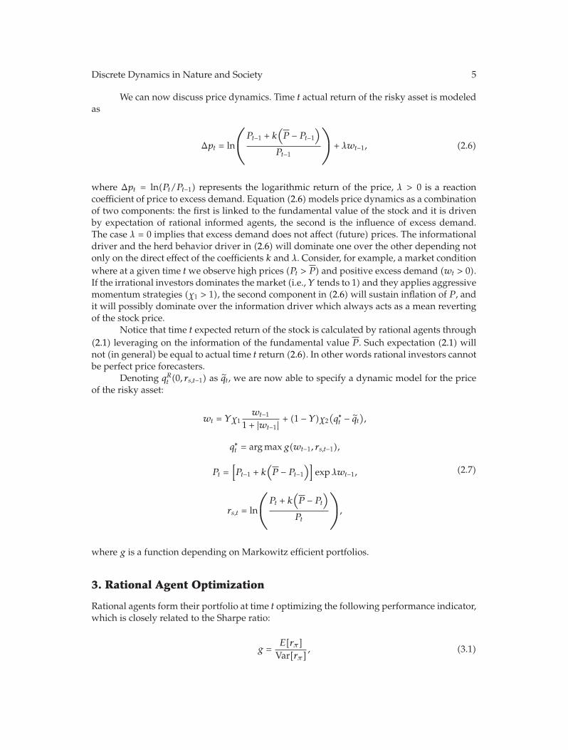
We can now discuss price dynamics. Time t actual return of the risky asset is modeledas
Δpt = ln
⎛⎜⎝
Pt−1 + k(P − Pt−1
)
Pt−1
⎞⎟⎠ + λwt−1, (2.6)
where Δpt = ln(Pt/Pt−1) represents the logarithmic return of the price, λ > 0 is a reactioncoefficient of price to excess demand. Equation (2.6)models price dynamics as a combinationof two components: the first is linked to the fundamental value of the stock and it is drivenby expectation of rational informed agents, the second is the influence of excess demand.The case λ = 0 implies that excess demand does not affect (future) prices. The informationaldriver and the herd behavior driver in (2.6) will dominate one over the other depending notonly on the direct effect of the coefficients k and λ. Consider, for example, a market conditionwhere at a given time twe observe high prices (Pt > P) and positive excess demand (wt > 0).If the irrational investors dominates the market (i.e., Y tends to 1) and they applies aggressivemomentum strategies (χ1 > 1), the second component in (2.6)will sustain inflation of P , andit will possibly dominate over the information driver which always acts as a mean revertingof the stock price.
Notice that time t expected return of the stock is calculated by rational agents through(2.1) leveraging on the information of the fundamental value P . Such expectation (2.1) willnot (in general) be equal to actual time t return (2.6). In other words rational investors cannotbe perfect price forecasters.
Denoting qRt (0, rs,t−1) as q̃t, we are now able to specify a dynamic model for the priceof the risky asset:
wt = Yχ1wt−1
1 + |wt−1| + (1 − Y )χ2(q∗t − q̃t
),
q∗t = argmax g(wt−1, rs,t−1),
Pt =[Pt−1 + k
(P − Pt−1
)]expλwt−1,
rs,t = ln
⎛⎜⎝
Pt + k(P − Pt
)
Pt
⎞⎟⎠,
(2.7)
where g is a function depending on Markowitz efficient portfolios.
3. Rational Agent Optimization
Rational agents form their portfolio at time t optimizing the following performance indicator,which is closely related to the Sharpe ratio:
g =E[rπ]Var[rπ]
, (3.1)
6 Discrete Dynamics in Nature and Society
where rπ is the return of a portfolio. The equivalence of the performance indicator g to theSharpe ratio [25] is clear: the variance of portfolio π is used instead of its standard deviation.As it is known in the literature (e.g., [26, page 626]), the indicators of the type as g in (3.1)show larger values for portfolios which are mean-variance efficient. It can be shown that anoptimal Sharpe ratio portfolio is also Markowitz efficient. To simplify the notation, next wewill denote the one period expected rate of return of the riskier asset rs,t−1 as rs and rf insteadof rf,t−1 for that of the bond whenever this will not generate confusion.
Based on standard portfolio theory, such objective can be expressed as the search of anoptimal weight vector q∗t satisfying:
q∗t = argmax g = argmaxqTt r
qTt Vt−1qt
, (3.2)
where rT = [rs rf] is the vector of stock and bond portfolio expected returns, qTt = [qt 1−qt]
the vector of their percentageweights, Vt−1 is the variance-covariance estimatedmatrix at timet − 1.
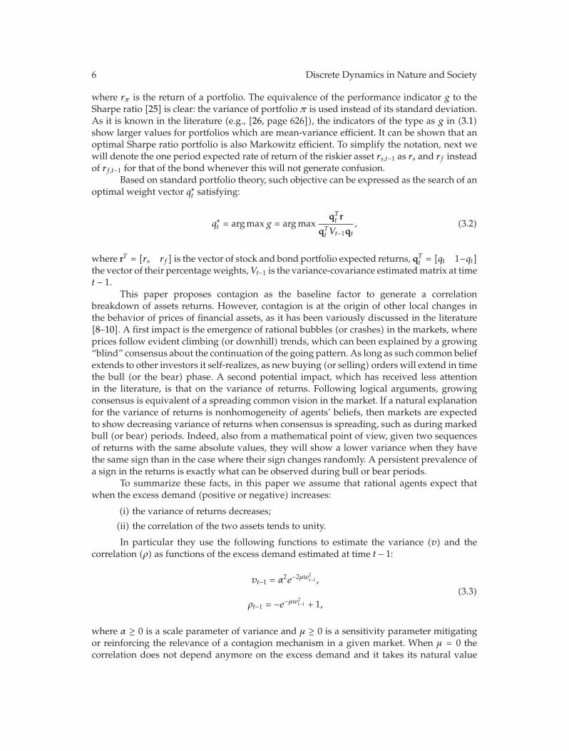
This paper proposes contagion as the baseline factor to generate a correlationbreakdown of assets returns. However, contagion is at the origin of other local changes inthe behavior of prices of financial assets, as it has been variously discussed in the literature[8–10]. A first impact is the emergence of rational bubbles (or crashes) in the markets, whereprices follow evident climbing (or downhill) trends, which can been explained by a growing“blind” consensus about the continuation of the going pattern. As long as such common beliefextends to other investors it self-realizes, as new buying (or selling) orders will extend in timethe bull (or the bear) phase. A second potential impact, which has received less attentionin the literature, is that on the variance of returns. Following logical arguments, growingconsensus is equivalent of a spreading common vision in the market. If a natural explanationfor the variance of returns is nonhomogeneity of agents’ beliefs, then markets are expectedto show decreasing variance of returns when consensus is spreading, such as during markedbull (or bear) periods. Indeed, also from a mathematical point of view, given two sequencesof returns with the same absolute values, they will show a lower variance when they havethe same sign than in the case where their sign changes randomly. A persistent prevalence ofa sign in the returns is exactly what can be observed during bull or bear periods.
To summarize these facts, in this paper we assume that rational agents expect thatwhen the excess demand (positive or negative) increases:
(i) the variance of returns decreases;
(ii) the correlation of the two assets tends to unity.
In particular they use the following functions to estimate the variance (v) and thecorrelation (ρ) as functions of the excess demand estimated at time t − 1:
vt−1 = α2e−2μw2t−1 ,
ρt−1 = −e−μw2t−1 + 1,
(3.3)
where α ≥ 0 is a scale parameter of variance and μ ≥ 0 is a sensitivity parameter mitigatingor reinforcing the relevance of a contagion mechanism in a given market. When μ = 0 thecorrelation does not depend anymore on the excess demand and it takes its natural value
Discrete Dynamics in Nature and Society 7
V
0
0.050.1
0.150.2
μ−4
−2w
24
0.02
0.04
0
(a)
0
0.050.1
0.150.2
μ−4
−2w
24
ρ
1
0.5
0
(b)
Figure 2:Graph of the variance (a) and of the correlation (b) as a function of excess demand and parameterμ.
(i.e., the one in force under normal regime), which we assume to be zero for the two assets ofour model (see Figure 2).
We obtain the following model for Vt−1:
Vt−1 =
⎡⎣ α2
1e−2μw2
t−1 α1α2e−2μw2
t−1ρt−1
α1α2e−2μw2
t−1ρt−1 α22e
−2μw2t−1
⎤⎦. (3.4)
In general the portfolio variance in (3.2) is a risk measure depending negatively on theabsolute value of excess demand.
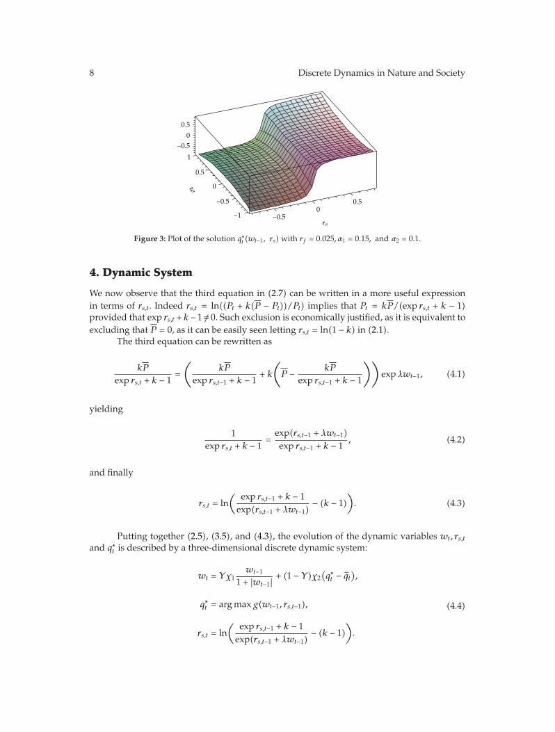
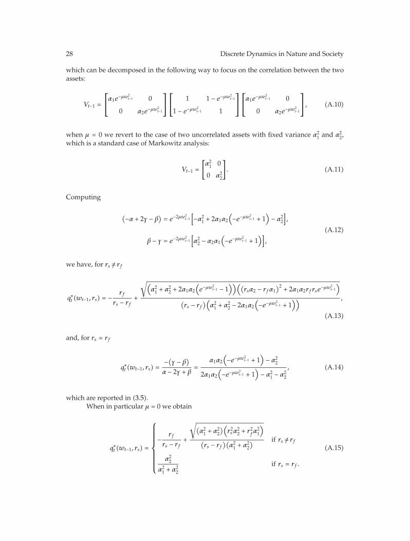
The optimization problem in (3.2), where Vt−1 is specified as in (3.4), has an explicitsolution (details are given in the appendices) depending on rs and wt−1:
q∗t (wt−1, rs)
=
⎧⎪⎪⎪⎪⎪⎪⎪⎪⎪⎨⎪⎪⎪⎪⎪⎪⎪⎪⎪⎩
− rf
rs − rf+
√(α21 + α2
2+2α1α2
(e−μw
2t−1 − 1
))((rsα2 − rfα1
)2+2α1α2rfrse−μw2
t−1)
(rs − rf
)(α21 + α2
2−2α1α2
(−e−μw2
t−1+1)) if rs/=rf ,
α1α2
(−e−μw2
t−1 + 1)−α2
2
2α1α2
(−e−μw2
t−1+1)−α2
1−α22
if rs=rf .
(3.5)
Figure 3 plots the solution (3.5) for some values of the other parameters.Recalling that q̃t = qRt (0, rs), from the expression (3.5) the value of q̃t can be easily
obtained as
q̃t = − rf
rs − rf+
√r2sα
22 + r2
fα21
(rs − rf
)√α21 + α2
2
. (3.6)
In Appendix A, we give the mathematical details of the solution to the optimizationproblem in (3.2) and briefly discuss its properties.
8 Discrete Dynamics in Nature and Society
−0.50
0.5
rs−1
−0.50
0.5
1
w
−0.5
0
0.5
Figure 3: Plot of the solution q∗t (wt−1, rs)with rf = 0.025, α1 = 0.15, and α2 = 0.1.
4. Dynamic System
We now observe that the third equation in (2.7) can be written in a more useful expressionin terms of rs,t. Indeed rs,t = ln((Pt + k(P − Pt))/Pt) implies that Pt = kP/(exp rs,t + k − 1)provided that exp rs,t + k − 1/= 0. Such exclusion is economically justified, as it is equivalent toexcluding that P = 0, as it can be easily seen letting rs,t = ln(1 − k) in (2.1).
The third equation can be rewritten as
kP
exp rs,t + k − 1=
(kP
exp rs,t−1 + k − 1+ k
(P − kP
exp rs,t−1 + k − 1
))expλwt−1, (4.1)
yielding
1exp rs,t + k − 1
=exp(rs,t−1 + λwt−1)exp rs,t−1 + k − 1
, (4.2)
and finally
rs,t = ln(
exp rs,t−1 + k − 1exp(rs,t−1 + λwt−1)
− (k − 1)). (4.3)
Putting together (2.5), (3.5), and (4.3), the evolution of the dynamic variables wt, rs,tand q∗t is described by a three-dimensional discrete dynamic system:
wt = Yχ1wt−1
1 + |wt−1| + (1 − Y )χ2(q∗t − q̃t
),
q∗t = argmax g(wt−1, rs,t−1),
rs,t = ln(
exp rs,t−1 + k − 1exp(rs,t−1 + λwt−1)
− (k − 1)).
(4.4)
Discrete Dynamics in Nature and Society 9
At time t, starting from rs,t−1 and wt−1, the third equation supplies the return expectedby rational agents at time t for the risky asset whereas the second one gives the optimalrational holdings q∗t . Finally we findwt by the first equation. Given the new valueswt and rs,tthe system can be iterated. Since q∗t is known given rs,t−1 andwt−1, we can eliminate the secondequation (which we analytically solve in Section 3) and finally consider a two-dimensionalmap (wt−1, rs,t−1) → (wt, rs,t) defined as
wt = Yχ1wt−1
1 + |wt−1| + (1 − Y )χ2(q∗t − q̃t
),
rs,t = ln(
exp rs,t−1 + k − 1exp(rs,t−1 + λwt−1)
− (k − 1)),
(4.5)
which will generate different evolution of the system depending both on the coefficients andthe initial condition (w0, rs,0). The coefficients of the system (4.5) are χ1, χ2, Y, k, and λ, whosepossible values have been already discussed, and, next to this, the coefficient μ influencingthe optimal portfolio q∗t .
Our discussion will focus on the influence of several coefficients on the behavior ofsystem (4.5). Besides this we will try to show how some initial conditions (excess demand inparticular) will influence the emergence of fundamental and non fundamental equilibria, aswell as price orbits.
4.1. Fixed Point Analysis
To simplify notations, let us introduce the unit time advancement operator “′” to reexpress(4.5):
w′ = Yχ1w
1 + |w| + (1 − Y )χ2(q∗ − q̃
),
r ′s = ln(exp rs + k − 1exp(rs + λw)
− (k − 1)).
(4.6)
The fixed points (w∗, r∗s) of system (4.6) will be named fundamental equilibria when thecondition P ∗ = P is verified, where P ∗ is the corresponding price to r∗s . Other equilibria willbe named non fundamental.
In the following proposition we show the existence of at least one equilibrium point(fundamental solution) for the system (4.6), given by the fixed points of the map (4.6).
Proposition 4.1. The pointQ0 = (w∗, r∗s) = (0, 0) is an equilibrium for the model (4.6) for all valuesof the parameters.
Proof. The following system is satisfied at the equilibrium:
w∗ = Yχ1w∗
1 + |w∗| + (1 − Y )χ2(q∗ − q̃
),
r∗s = ln(
exp r∗s + k − 1exp(r∗s + λw∗)
− (k − 1)),
(4.7)
10 Discrete Dynamics in Nature and Society
rearranging terms, the second equation becomes:
exp r∗s + k − 1 =exp r∗s + k − 1exp(r∗s + λw∗)
, (4.8)
yielding
exp(r∗s + λw∗) = 1. (4.9)
Solving such equality, system (4.7) is equivalent to
w∗ = Yχ1w∗
1 + |w∗| + (1 − Y )χ2(q∗ − q̃
),
r∗s = −λw∗.
(4.10)
When w∗ = 0, the first equation is satisfied, since q̃ = qR(0, rs) by definition and the secondequation yields the solution r∗s = 0 for every λ/= 0. This completes the proof.
Observe that when Pt = P then rs = 0, as it can be verified by inspection of (2.1).Rational agents fix to zero the expected return of the risky asset when current price is equal toits fundamental value. So Pt = P coupled withwt = 0 and rs = 0 is a fundamental equilibriumsolution for (2.7).
When rs = r∗ /= 0 eventual other equilibria have the form (w∗,−λw∗), where theexpression of w∗ is implicitly described by the first equation in (4.10).
Given that rs is obtained through a monotone transformation of price Pt, we do notrisk losing possible solutions of the original system.
4.2. Local Stability Analysis of the Fundamental Solution (0, 0)
4.2.1. The Contagion Effect
In the previous paragraph we have shown that Q0 = (w∗, r∗s) = (0, 0) is an equilibrium pointfor the model (4.6); now we want to study the existence of other equilibria and their stabilitywhen all agents act following the market demand (Y = 1). In this case the system (4.6)becomes
w′ = χ1w
1 + |w| ,
r ′s = ln(exp rs + k − 1exp(rs + λw)
− (k − 1)),
(4.11)
as the rational component vanishes. Following the standard dynamic systems theory (see[27]), the local stability analysis of the fixed point is based on the location, in the complexplane, of the eigenvalues of the Jacobian matrix (for this and the other cases we refer to
Discrete Dynamics in Nature and Society 11
Appendix B for detailed calculations needed to construct the Jacobian matrix):
J(0, 0) =
[χ1 0
−kλ 1 − k
]. (4.12)
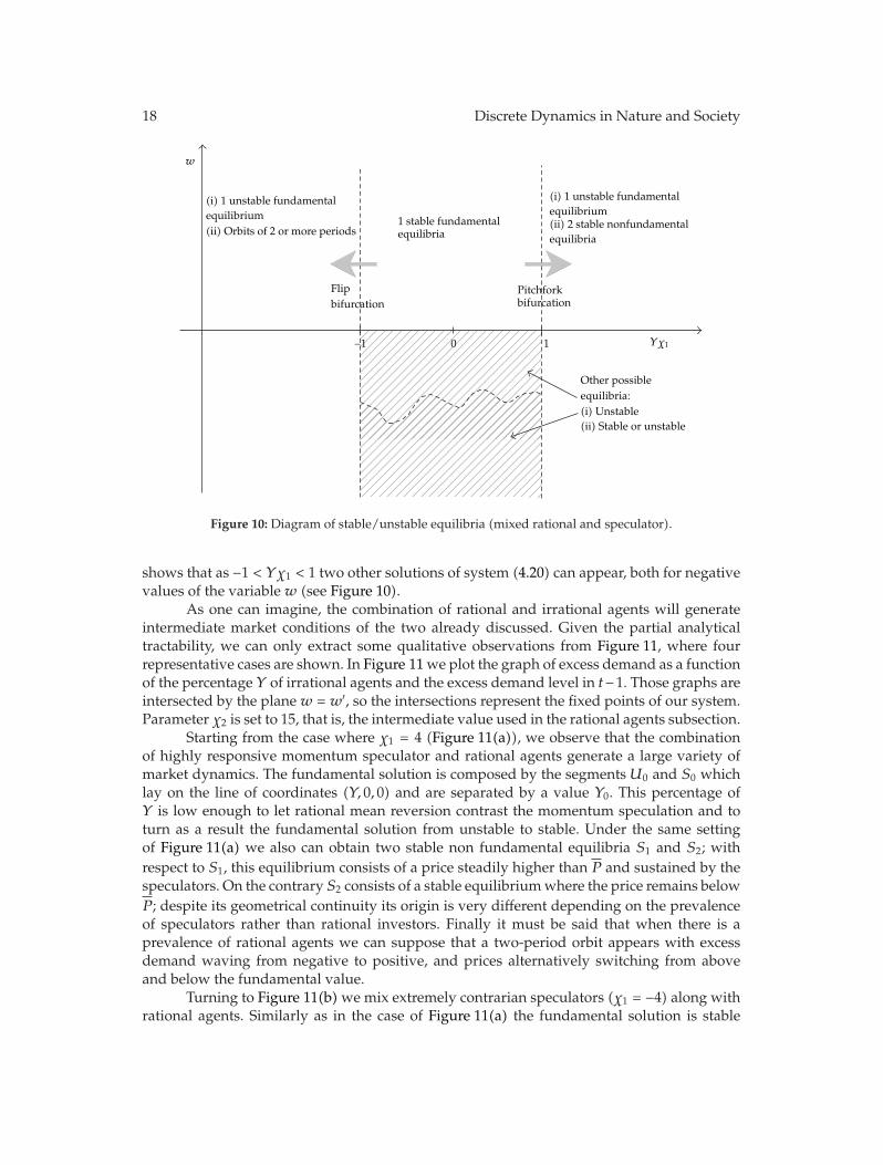
The eigenvalues are λ1 = χ1 and λ2 = 1 − k; observe that λ2 is always less than 1 inabsolute value, given that k ∈ (0, 1) under the hypothesis of our model; then the stabilityanalysis of (0, 0) depends on the λ1 eigenvalue (i.e., on the value of the parameter χ1).
More precisely, Q0 = (0, 0) is a stable equilibrium if |χ1| < 1. χ1 = 1 and χ1 = −1 arebifurcation values. When |χ1| > 1 the point Q0 becomes unstable and different situations canoccur depending on cases χ1 > 1 and χ1 < −1. When χ1 > 1, two new equilibria w∗
1 = χ1 − 1andw∗
2 = −χ1 +1 appear corresponding to the pointsQ1 = (χ1 −1,−λ(χ1 −1)) andQ2 = (−χ1 +1,−λ(−χ1 + 1)) in the phase plane (w, rs), as a consequence of the bifurcation occurring whenχ1 = 1. The nature of this bifurcation can be examined by studying the one-dimensional fam-ily of maps w′ = f(w, χ1), where f(w, χ1) = χ1(w/(1 + |w|)) depending on the parameter χ1.
At (0, 1) we obtain
∂f(0, 1)∂w
= 1,∂2f(0, 1)∂w∂χ1
= 1,∂3f(0, 1)∂w3
= 6, (4.13)
so the conditions (4.13) guarantee that (0, 1) determines a supercritical pitchfork bifurcation.A value of χ1 > 1 shows the tendency of the uninformed agents to overreact to
signals about excess demand. Whenw is just greater than 0, they respond raising next perioddemand further until level w∗
1 = χ1 − 1 is reached. At that point excess demand stabilizes.At the same time the equity price grows to P ∗
1 = k/(e−λ(χ1−1) − 1 + k)P . Since P ∗1 > P ,
if excess demand is positive the factor k/(e−λ(χ1−1) − 1 + k) is greater than 1; this implies1 < χ1 < ((λ − ln(1 − k))/λ). So a further condition χ1 < ((λ − ln(1 − k))/λ) is also required toguarantee market consistency. Mean reverting expectation of rational investors r∗s = −λ(χ1−1)is negative when P ∗
1 > P . However, price remains high when Y = 1 no rational investors arepresent in the market to balance the positive excess demand generated by the speculators.
On the contrary when excess demand is negative, uninformed agents respond sellingeven more until the level w∗
2 = 1 − χ1 is reached. Following similar arguments when w < 0an equilibrium price is reached at price P ∗
2 = k/(e−λ(1−χ1) − 1 + k)P which must be less thanP under standard market conditions. The inequality χ1 > (λ − ln(1 − k))/λ must be satisfiedand corresponding rational expected return r∗s = −λ(1 − χ1) is positive.
In order to study the local stability of the new fixed pointsQ1 = (χ1−1,−λ(χ1−1)) andQ2 = (−χ1 + 1,−λ(−χ1 + 1))we compute the eigenvalues of the Jacobian matrix in Q1 and Q2.
Being
J(Q1) =
⎡⎣
1χ21
0
−λ + λ(k − 1)eλ(χ1−1) (1 − k)eλ(χ1−1)
⎤⎦, (4.14)
the eigenvalues are λ1 = 1/χ1 and λ2 = (1 − k)eλ(χ1−1); as we are examining the case χ1 > 1, λ1is always in absolute value less than 1; |λ2| < 1 when (1 − k)eλ(χ1−1) < 1 that implies χ1 <(λ− ln(k−1))/λ. As we already observed, in the casew > 0 this inequality is always satisfied,as coherent with the condition of market consistency.

12 Discrete Dynamics in Nature and Society
With similar calculations
J(Q2) =
⎡⎢⎢⎣
1χ21
0
−λ + λ(k − 1)eλ(−χ1+1) (1 − k)eλ(−χ1+1)
⎤⎥⎥⎦, (4.15)
with eigenvalues λ1 = 1/χ1 and λ2 = (1 − k)eλ(−χ1+1); the first one is always less than 1 inabsolute value whereas |λ2| < 1 when (1− k)eλ(−χ1+1) < 1, which implies χ1 > (λ− ln(1− k))/λthat is always satisfied.
PointsQ1 andQ2 correspond to two nonfundamental asymptotically stable equilibria.Finally, if χ1 = −1 a flip bifurcation occurs and when χ1 < −1 a two-period cycle
appears in the phase plane (w, rs), whose elements are {w∗3,w
∗4},w∗
3 = χ1 + 1,w∗4 = −χ1 − 1.
These elements can be identified through a double iteration of the system (4.11):
w′′ = χ21
w(1 +
∣∣χ1(w/(1 +w))∣∣)(1 + |w|)
r ′′s = ln
( (exp rs + k − 1
)/ exp(rs + λw)((
exp rs + k − 1)/ exp(rs + λw) − (k − 1)
)expλχ1(w/(1 + |w|)) − (k − 1)
),
(4.16)
yielding two fixed points Q3 = (−χ1 − 1, ln((1 + (1 − k)eλ(χ1+1))/(eλ(χ1+1) + 1 − k))) and Q4 =(χ1 + 1, ln((1 + (1 − k)e−λ(χ1+1))/(e−λ(χ1+1) + (1 − k)))).
As a consequence of the contrarian attitude of this market (χ1 < 0), positive excessdemand in period t turns into negative demand in period t + 1. In particular the values ofthe excess demand orbit are w∗
3 = −χ1 − 1 and w∗4 = χ1 + 1. The pressure on the price will
accordingly wave from up and down. Corresponding market prices oscillate between twovalues P3 < P < P4. In particular we have
P3 =eλ(χ1+1) + (1 − k)
2 − kP < P ,
P4 =e−λ(χ1+1) + 1 − k
2 − kP > P .
(4.17)
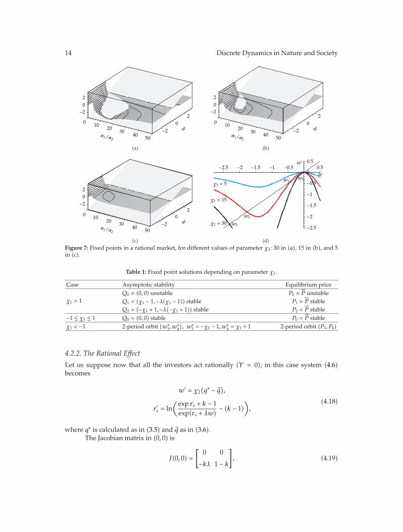
Appendix C shows all required calculations and other details of such results.The analysis of the two-period orbit stability is not an easy task, as must be done by
studying the stability of fixed pointsQ3 andQ4; however, simulation analysis reveals a stableorbit (see Figures 4 and 5).
Figure 6 shows the equilibria stability in an example with different values ofparameters χ1. Figure 6(a) shows the graph of f(w, χ1) for two values of χ1; from χ1 = 0.8 toχ1 = 4 a Pitchfork bifurcation occurs. Figure 6(b) shows the graph of f(w, χ1) for two valuesof χ1 (i.e., −0.8 and −4) and the equilibrium valuesw∗ included in the two-periods orbit. Theconvergence path is clearly pointing to the origin when χ1 = −0.8; vice versa it draws a cycleof period two when χ1 = −4.
We summarize the results of this section in Table 1.
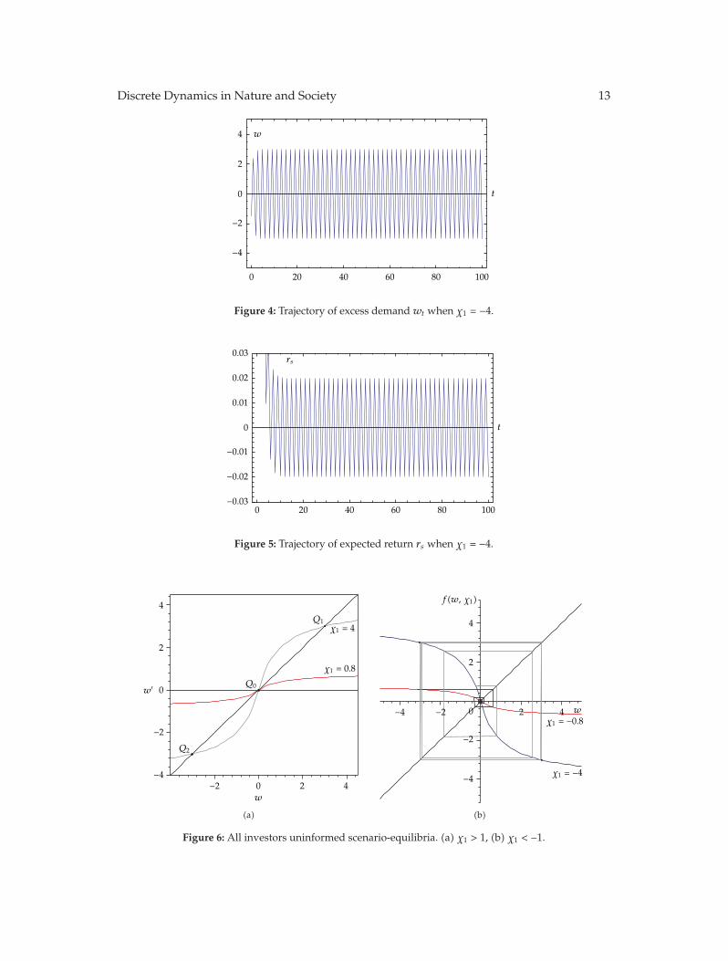
Discrete Dynamics in Nature and Society 13
w
0 20 40 60 80 100
−4
−2
0
2
4
t
Figure 4: Trajectory of excess demand wt when χ1 = −4.
0 20 40 60 80 100
t
rs0.03
0.02
0.01
0
−0.01
−0.02
−0.03
Figure 5: Trajectory of expected return rs when χ1 = −4.
−4
−2
0
2
4
w′
−2 0 2 4w
Q0
Q1
Q2
χ1 = 4
χ1 = 0.8
(a)
−4
−2
0
2
4
−4 −2 2 4 wχ1 = −0.8
χ1 = −4
f(w, χ1)
(b)
Figure 6: All investors uninformed scenario-equilibria. (a) χ1 > 1, (b) χ1 < −1.
14 Discrete Dynamics in Nature and Society
−202
010
2030
4050
wα1/α2
−20
2
(a)
−202
0 1020
30 4050
wα1/α2
−20
2
(b)
−202
0 1020
3040
50
wα1/α2
−20
2
(c)
w
−2.5 −2 −1.5 −1 −0.50
0.5w’
−2.5
−1.5
−1
−0.5
0.5
−2χ2 = 30
χ2 = 15
χ2 = 5
w2
w1w1
w2
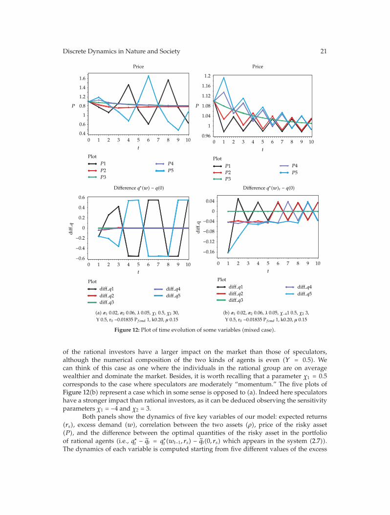
(d)Figure 7: Fixed points in a rational market, for different values of parameter χ2: 30 in (a), 15 in (b), and 5in (c).
Table 1: Fixed point solutions depending on parameter χ1.
Case Asymptotic stability Equilibrium price
χ1 > 1Q0 = (0, 0) unstable P0 = P unstableQ1 = (χ1 − 1,−λ(χ1 − 1)) stable P1 > P stableQ2 = (−χ1 + 1,−λ(−χ1 + 1)) stable P2 < P stable
−1 ≤ χ1 ≤ 1 Q0 = (0, 0) stable P0 = P stableχ1 < −1 2-period orbit {w∗
3,w∗4}, w∗
3 = −χ1 − 1,w∗4 = χ1 + 1 2-period orbit (P3,P4)
4.2.2. The Rational Effect
Let us suppose now that all the investors act rationally (Y = 0); in this case system (4.6)becomes
w′ = χ2(q∗ − q̃
),
r ′s = ln(exp rs + k − 1exp(rs + λw)
− (k − 1)),
(4.18)
where q∗ is calculated as in (3.5) and q̃ as in (3.6).The Jacobian matrix in (0, 0) is
J(0, 0) =
[0 0
−kλ 1 − k
], (4.19)

Discrete Dynamics in Nature and Society 15
whose eigenvalues are λ1 = 0 and λ2 = 1 − k. Since under standard assumptions k ∈(0, 1), the eigenvalues are always less than 1 in absolute value, the solution (0, 0) is alwaysasymptotically locally stable for every value of the parameter χ2.
This can be easily seen also from system (4.18). When all rational investors start froma zero excess demand (wt−1 = 0) their optimal demand for the risky assets is q∗ = q̃ (by thedefinition of q̃). As a consequence next period excess demand is again wt = 0.
Inspecting again system (4.18)we obtain that rs,t = 0, which implies that current priceof the risky asset is equal to its fundamental value (Pt = P).
Outside the fundamental solution the inspection of other fixed points is by far lesssimple. Actually some simulation and numerical analysis can be the only way to inspectother possible equilibria resulting in a market fully populated by informed agents. Figure 7represents w′ as a function of w and the parameter α1, that is, the one-dimensional family ofmaps w′ = g(w, α1). In all three panels the plane w′ = w always intersects g(w, α1) at w = 0,that is corresponding to the fundamental solution. However it is also possible to observe thatfor values of parameter α1 less than about 0.05 (panel (a)) and 0.025 (panel (b)), g(w, α1)intersects the plane w′ = w in other two points, call them w1 and w2. Corresponding to suchintersections, we see in Figures 7(a) and 7(b), that the graph of g(w, α1) “vanishes” below thebisecting plane w′ = w. See also Figure 7(d) where these intersections (w1 and w2) are alsoshown for a fixed value of parameter α1. For simple analytical properties of g(w, α1) pointsw1 can never be a stable solution. On the contraryw2 can be both a stable or unstable solution.In the cases represented in Figure 7(d), where χ2 = 30 and χ2 = 15 we can observe that w2 is,respectively, an unstable and stable solution.
Besides a stable non equilibrium fixed point, the full rational scenario can also generatestable orbits of various periods. The occurrence of such a situation can be attributed toparticular combinations of the parameters and the initial values of the system. Markets can behit occasionally by unexpected good (bad) news, shifting the fundamental value of the riskyasset and attracting (chasing away) new significant portions of demand. Rational traders canthen try to anticipate a possible demand rush and change the correlation estimate based on(3.3). Depending on the values of some parameters, even a market dominated by rationalinvestors can be captured into dynamics keeping the system steadily out of equilibrium.Paradoxically at the origin of such imbalance is a “rational” yet myopic intent to preventit. Indeed each agent optimizes rationally a private portfolio problem, without consideringthat many individuals, with an identical intent, are jointly swelling the order book on thesame side.
In Figure 8 panels (a.1) and (a.2) show the trajectories of stable orbits of period 5.In particular panel (a.1) shows the corresponding time series of rs and w while in panel(a.2) the trajectories are plotted in the phase plane. The emergence of orbits tend to occurespecially when coefficient χ2 is high (i.e., high impact on demand as a consequence ofportfolio adjustments), when the ratio α1/α2 ↓ 1 (i.e., small difference in volatility betweenthe two traded assets), and coefficient μ is high (i.e., the correlation breakdown effectincreases).
When χ2 assumes intermediate values such as 20 and the ratio α1/α2 lays in an intervalsimilar to that already discussed in Figure 7, the system allows the emergence of two stableequilibria (see Figure 8 panels (b.1) and (b.2)): one is the fundamental solution (w = 0, rs =0,P = P), the other is a non-fundamental equilibrium (with w < 0, rs > 0 and P < P). Finallyif the influence parameter is low enough such as χ2 = 5 (see Figure 8(c)), then the only fixedpoint appears to be the fundamental solution whatever the starting point.

16 Discrete Dynamics in Nature and Society
w
−40
−30
−20
−10
0
10
20
0 10 20 30 40 50 60
r−0.100.10.20.30.40.50.60.70.80.9
11.1
t
w
r r
0
0.2
0.4
0.6
0.8
1
1.2
1.4
−40 −30 −20 −10 0 10 20
w
(a.2) (a.1)
k 0.2λ, 0.05χ1, 0.5χ2, 40Y , 0rf , 0.002α1, 0.2α2, 0.004μ0.4 k 0.2λ, 0.05χ1, 0.5χ2, 40Y , 0rf , 0.02α1, 0.02α2, 0.004μ0.4
(a)
w
−5
−4
−3
−2
−1
t
0 10 20 30 40 50 60
r
−0.020
0.02
0.04
0.06
0.08
0.1
0.12
0.14
0.16
0.18
w
r r
−0.04−0.02
0
0.02
0.04
0.06
0.08
0.1
0.12
0.14
0.16
0.18
w
−5 −4 −3 −2 −1 0
(b.1) (b.2)
k 0.2λ, 0.05χ1, 0.5χ2, 20Y , 0rf , 0.02α1, 0.02α2, 0.0004μ0.4 k 0.2λ, 0.05χ1, 0.5χ2, 20Y,0rf , 0.02α1, 0.02α2, 0.0004μ0.4
(b)
w
−1.6
−1.4
−1.2
−1
−0.8
−0.6
−0.4
−0.2
0
r
−0.02−0.018−0.016−0.014−0.012−0.01−0.008−0.006−0.004−0.00200.0020.0040.0060.0080.01
rw
t
0 10 20 30 40 50 60
r
−0.04−0.02
0
0.02
0.04
0.06
0.08
0.1
0.12
0.14
0.16
w
−1.4 −1.2 −1 −0.8 −0.6 −0.4 −0.2 0 0.2 0.4
(c.1) (c.2)
k 0.2λ, 0.05χ1, 0.5χ2, 5Y , 0rf , 0.02α1, 0.02α2, 0.004μ0.2 k 0.2λ, 0.05χ1, 0.5χ2, 5Y , 0rf , 0.02α1, 0.02α2, 0.004μ0.2
(c)Figure 8: Trajectorieswt (excess demand) for χ2 = 30 (a), χ2 = 15 (b), and χ2 = 5 (c).

Discrete Dynamics in Nature and Society 17
−6
−4
2
4
−4 −3 −2 −10
1 2 3 4
w
w’
−2Yχ1 = 2
Yχ1 = 0.04
Figure 9: Pitchfork bifurcation: when Yχ1 > 1 (0, 0) becomes unstable and two new fixed points appear.
4.2.3. Mixed Rational and Speculators Market
In the more general case the market is composed of a positive percentage of both informedand uninformed agents; in this case the market dynamics are described by the followingsystem:
w′ = Yχ1w
1 + |w| + (1 − Y )χ2(q∗t − q̃
),
r ′s = ln(exp rs + k − 1exp(rs + λw)
− (k − 1)).
(4.20)
The Jacobian matrix in (0, 0) is
J(0, 0) =
[Yχ1 0
−kλ 1 − k
], (4.21)
with eigenvalues λ1 = Yχ1, λ2 = 1 − k.The situation we can observe is due to the convex combination (with coefficient Y )
of the two different effects (contagion and rational), thus the analysis of the fundamentalequilibrium (0, 0) is similar to the analysis already done: taking k ∈ (0, 1), the condition|λ2| < 1 is always satisfied, the solution (0, 0) is locally asymptotically stable if |Yχ1| < 1.When |Yχ1| > 1, the equilibrium point becomes unstable; Yχ1 = −1 and Yχ1 = 1 arebifurcation values. In particular, when Yχ1 = 1 a pitchfork bifurcation occurs and forYχ1 > 1 the equilibrium (0, 0) loses stability whereas two new equilibria, having the form(w,−λw), appear. Figure 9 depicts this situation for χ2 = 5 and for suitable values of theother parameters.
When Yχ1 = −1 a flip bifurcation occurs, and a 2-period cycle appears as a solution ofthe system (4.20).
As pointed before, in the case |Yχ1| < 1 the analytical study allows us to conclude thatthe solution (0, 0) is always locally asymptotically stable, but we have no other informationconcerning the existence of eventual other fixed points; actually, some simulation study
18 Discrete Dynamics in Nature and Society
−1 0 1
w
Flipbifurcation
Pitchforkbifurcation
Yχ1
(i) 1 unstable fundamentalequilibrium(ii) Orbits of 2 or more periods
1 stable fundamentalequilibria
(ii) 2 stable nonfundamentalequilibria
Other possibleequilibria:(i) Unstable(ii) Stable or unstable
(i) 1 unstable fundamentalequilibrium
Figure 10: Diagram of stable/unstable equilibria (mixed rational and speculator).
shows that as −1 < Yχ1 < 1 two other solutions of system (4.20) can appear, both for negativevalues of the variable w (see Figure 10).
As one can imagine, the combination of rational and irrational agents will generateintermediate market conditions of the two already discussed. Given the partial analyticaltractability, we can only extract some qualitative observations from Figure 11, where fourrepresentative cases are shown. In Figure 11 we plot the graph of excess demand as a functionof the percentage Y of irrational agents and the excess demand level in t−1. Those graphs areintersected by the plane w = w′, so the intersections represent the fixed points of our system.Parameter χ2 is set to 15, that is, the intermediate value used in the rational agents subsection.
Starting from the case where χ1 = 4 (Figure 11(a)), we observe that the combinationof highly responsive momentum speculator and rational agents generate a large variety ofmarket dynamics. The fundamental solution is composed by the segments U0 and S0 whichlay on the line of coordinates (Y, 0, 0) and are separated by a value Y0. This percentage ofY is low enough to let rational mean reversion contrast the momentum speculation and toturn as a result the fundamental solution from unstable to stable. Under the same settingof Figure 11(a) we also can obtain two stable non fundamental equilibria S1 and S2; withrespect to S1, this equilibrium consists of a price steadily higher than P and sustained by thespeculators. On the contrary S2 consists of a stable equilibriumwhere the price remains belowP ; despite its geometrical continuity its origin is very different depending on the prevalenceof speculators rather than rational investors. Finally it must be said that when there is aprevalence of rational agents we can suppose that a two-period orbit appears with excessdemand waving from negative to positive, and prices alternatively switching from aboveand below the fundamental value.
Turning to Figure 11(b)we mix extremely contrarian speculators (χ1 = −4) along withrational agents. Similarly as in the case of Figure 11(a) the fundamental solution is stable

Discrete Dynamics in Nature and Society 19
−4
3
w0
1
Y
−5
0w’
S1
S2 S0
U0
U1
(a) χ1 = 4
−4
3
w0
1
Y
−5
0w’
S1
S0
U0
U1
(b) χ1 = −4
−4
3
w0
1
Y
−5
0w’
S1
S0
U1
(c) χ1 = 0.8
−4
3
w
0
1
Y
−5
0
w’
S1
S0
U1
(d) χ1 = −0.8
Figure 11: Different behaviours of agents for χ2 = 15 and many values of χ1.
only if there is a large presence of rationals (segment S0). Besides, the large presence ofrationals can also determine non fundamental solutionsU1 (unstable) and S1 (stable), as longas the excess demand goes lower than zero, which we have already discussed. If contrarianspeculators prevail, we can suppose that the two-period orbit appears.
In Figure 11(c) we combine moderately momentum speculators (χ1 = 0.8) withrational agents. As we expect from the separate analysis of the two kinds of agents, thefundamental solution (S0) is always stable; surprisingly enough, the only source of possiblenon equilibrium solutions is represented by the large presence of rational agents. As theexcess demand lowers below zero, two equilibrium solutions appears, U1 (unstable) andS1 (stable). As in the previous cases, S1 is characterized by a price of the risky asset lowerthan its fundamental value.
In Figure 11(d) (χ1 = −0.8) the market conditions are quite similar to those inFigure 11(c), even though speculation is moderately contrarian in this case. The fundamentalsolution S0 is stable for any level of Y , the emergence of non fundamental equilibrium S1 isstill represented by a large presence of rational agents, even though less are required than inthe case of Figure 11(c). The contrarian speculator, indeed, enhances the emergence of thisnon fundamental solution.
Figure 12 shows several interesting properties of our model. It is organized in twocolumns of five plots on the left (Figure 12(a)) and five on the right (Figure 12(b)). Inparticular, Figure 12(a) refers to a case where rational investors are more critical thenspeculators: parameter χ2 (χ2 = 30) is much larger than χ1 (χ1 = 0.5). In this way the decisions

20 Discrete Dynamics in Nature and Society
rs
−0.10−0.06−0.020.02
0.06
0.1
0.14
0.18
0 1 2 3 4 5 6 7 8 9 10
Expected returns
Plotrs1
rs2
rs3
rs4
rs5
t
0 1 2 3 4 5 6 7 8 9 10
Expected returns
Plot
rs1
rs2
rs3
rs4
rs5
t
rs
−0.036−0.031−0.026−0.021−0.016−0.011−0.006−0.0010.004
0.009
t
Excess demand
w
−8−6−4−202468
Plotw1
w2
w3
w4
w5
0 1 2 3 4 5 6 7 8 9 10 0 1 2 3 4 5 6 7 8 9 10
Excess demand
Plotw1
w2
w3
w4
w5
w
−2
−1
0
1
2
t
0 1 2 3 4 5 6 7 8 9 10
Correlation between assets
Plotρ1 ρ4
ρ2
ρ3
ρ5
Corr
t
0
0.05
0.2
0.3
0.4
0.5
ρ
00.10.20.30.40.50.60.70.80.91
0 1 2 3 4 5 6 7 8 9 10
Correlation between assets
Plotρ1 ρ4ρ2
ρ3ρ5
t
Figure 12: Continued.
Discrete Dynamics in Nature and Society 21
0 1 2 3 4 5 6 7 8 9 10
Price
t
PlotP1P2P3
P4P5
P
0.96
1
1.04
1.08
1.12
1.16
1.2
P
0.4
0.6
0.8
1
1.2
1.4
1.6
0 1 2 3 4 5 6 7 8 9 10
Price
t
PlotP1P2P3
P4P5
Difference q∗(w) − q(0)
diff
q
−0.6−0.4−0.2
0
0.2
0.4
0.6
Plotdiff q1diff q2diff q3
diff q4diff q5
0 1 2 3 4 5 6 7 8 9 10
t
Plotdiff q1diff q2diff q3
diff q4diff q5
0 1 2 3 4 5 6 7 8 9 10
Difference q∗(w)t − q(0)
diff
q
−0.16−0.12−0.08−0.04
0
0.04
t
(b) α1 0.02, α2 0.06, λ 0.05, χ−41 0.5, χ2 3,Y 0.5, r0 −0.01835 Pfond 1, k0.20, μ 0.15
(a) α1 0.02, α2 0.06, λ 0.05, χ1 0.5, χ2 30,Y 0.5, r0 −0.01835 Pfond 1, k0.20, μ 0.15
Figure 12: Plot of time evolution of some variables (mixed case).
of the rational investors have a larger impact on the market than those of speculators,although the numerical composition of the two kinds of agents is even (Y = 0.5). Wecan think of this case as one where the individuals in the rational group are on averagewealthier and dominate the market. Besides, it is worth recalling that a parameter χ1 = 0.5corresponds to the case where speculators are moderately “momentum.” The five plots ofFigure 12(b) represent a case which in some sense is opposed to (a). Indeed here speculatorshave a stronger impact than rational investors, as it can be deduced observing the sensitivityparameters χ1 = −4 and χ2 = 3.
Both panels show the dynamics of five key variables of our model: expected returns(rs), excess demand (w), correlation between the two assets (ρ), price of the risky asset(P), and the difference between the optimal quantities of the risky asset in the portfolioof rational agents (i.e., q∗t − q̃t = q∗t (wt−1, rs) − q̃t(0, rs) which appears in the system (2.7)).The dynamics of each variable is computed starting from five different values of the excess
22 Discrete Dynamics in Nature and Society
Stan
darddev
iation
stockindex Same week
8days later
0
0.002
0.004
0.006
0.008
0.01
0.012
0.014
−6 −5 −4 −3 0 3 4 5 6
Prevailing signs of the US Datastream Stock Index returnobserved over a week period
(a)
Same week
8days later
Stan
darddev
iation
bond
price
−6 −5 −4 −3 0 3 4 5 60.0036
0.0038
0.004
0.0042
0.0044
0.0046
0.0048
0.005
Prevailing signs of the US Datastream Stock Index returnobserved over a week period
(b)
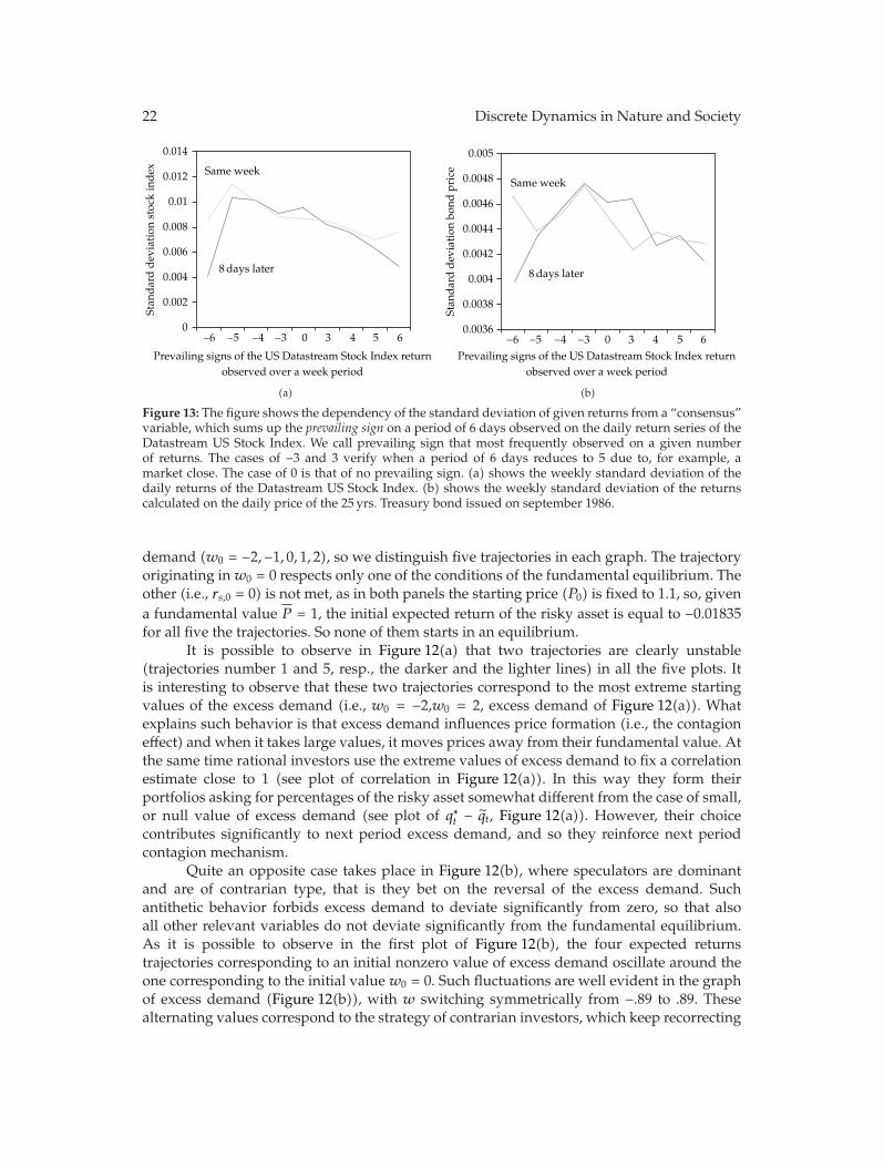
Figure 13: The figure shows the dependency of the standard deviation of given returns from a “consensus”variable, which sums up the prevailing sign on a period of 6 days observed on the daily return series of theDatastream US Stock Index. We call prevailing sign that most frequently observed on a given numberof returns. The cases of −3 and 3 verify when a period of 6 days reduces to 5 due to, for example, amarket close. The case of 0 is that of no prevailing sign. (a) shows the weekly standard deviation of thedaily returns of the Datastream US Stock Index. (b) shows the weekly standard deviation of the returnscalculated on the daily price of the 25 yrs. Treasury bond issued on september 1986.
demand (w0 = −2,−1, 0, 1, 2), so we distinguish five trajectories in each graph. The trajectoryoriginating inw0 = 0 respects only one of the conditions of the fundamental equilibrium. Theother (i.e., rs,0 = 0) is not met, as in both panels the starting price (P0) is fixed to 1.1, so, givena fundamental value P = 1, the initial expected return of the risky asset is equal to −0.01835for all five the trajectories. So none of them starts in an equilibrium.
It is possible to observe in Figure 12(a) that two trajectories are clearly unstable(trajectories number 1 and 5, resp., the darker and the lighter lines) in all the five plots. Itis interesting to observe that these two trajectories correspond to the most extreme startingvalues of the excess demand (i.e., w0 = −2,w0 = 2, excess demand of Figure 12(a)). Whatexplains such behavior is that excess demand influences price formation (i.e., the contagioneffect) and when it takes large values, it moves prices away from their fundamental value. Atthe same time rational investors use the extreme values of excess demand to fix a correlationestimate close to 1 (see plot of correlation in Figure 12(a)). In this way they form theirportfolios asking for percentages of the risky asset somewhat different from the case of small,or null value of excess demand (see plot of q∗t − q̃t, Figure 12(a)). However, their choicecontributes significantly to next period excess demand, and so they reinforce next periodcontagion mechanism.
Quite an opposite case takes place in Figure 12(b), where speculators are dominantand are of contrarian type, that is they bet on the reversal of the excess demand. Suchantithetic behavior forbids excess demand to deviate significantly from zero, so that alsoall other relevant variables do not deviate significantly from the fundamental equilibrium.As it is possible to observe in the first plot of Figure 12(b), the four expected returnstrajectories corresponding to an initial nonzero value of excess demand oscillate around theone corresponding to the initial valuew0 = 0. Such fluctuations are well evident in the graphof excess demand (Figure 12(b)), with w switching symmetrically from −.89 to .89. Thesealternating values correspond to the strategy of contrarian investors, which keep recorrecting
Discrete Dynamics in Nature and Society 23
their previous move. In this way they end up with neutralizing most of their influence onprices, which in the long run revert towards their fundamental value. Such reversion canbe observed in the graph of price (Figure 12(b)). Though prices keep oscillating, the centerof these trajectories tends indeed to P = 1. In the end expected returns, prices, and excessdemand enter into a 2-period orbit similarly to the case when only (contrarian) speculatorspopulate the market. It is finally worth noticing that contrarian speculators and rationalagents tend indeed to neutralize each other. This can be observed comparing q∗t − q̃t andw which (after the first 8 periods) regularly take opposite signs.
4.3. Some Empirical Evidence
We report some empirical evidence which justify part of the assumptions of this work, withparticular reference to the form of the variance-covariance estimate used by rational agentsin (3.4). We collected the daily series of the of the US Stock Index calculated by Datastreamand the daily series of prices of US Treasury bond, 25 years maturity, issued on September1986, for the period from janurary-1-1993 to March-31-2008.
To the purpose of obtaining a proxy of the excess demand for the stock index, weelaborated a “consensus” variable based on the number of signs observed on the returns ona period of 6 days. In particular we considered the following summations:
#+t =5∑i=0
IR+(rt−i),
#−t =5∑i=0
IR−(rt−i),
(4.22)
where I(·) is the indicator function and rt is the return observed on the Datastream US StockIndex. Those summations count, respectively, the number of positive and negative returnsoccurred in the six days from t back to t − 5 (including t). Our consensus variable is thendefined as
ct =
⎧⎪⎪⎪⎨⎪⎪⎪⎩
#+t if #+t > #−t ,
−#−t if #+t < #−t ,
0 if #+t = #−t .
(4.23)
The reason why ct can be considered as a proxy for the excess demand at time t is the it canbe argued that when contagion mechanism is acting in a market during a given period, thena sign of the returns should clearly prevail, depending on the kind of sentiment. Moreover,it can be assumed that the stronger a sign is prevailing in a given period, the stronger is thecontagion hitting a market.
Figure 13 shows the graph of the weekly standard deviation of the returns of the twoseries as a function of the consensus variable. More precisely letting ct the consensus observedin t, the standard deviation has been calculated on two periods of time: the “same week”(i.e., between t and t − 4) and “8 days later” (i.e., between t + 8 and t). It can be noticedthat the standard deviation of the returns of both the series in usually higher when there isno strong sign prevalence, that is, when ct = {−4,−3.0, 3, 4} (the cases −3 and 3 arise whenone day out of six corresponds to a market close). The same statistic clearly lowers when

24 Discrete Dynamics in Nature and Society
−0.1
0
0.1
0.2
0.3
0.4
0.5
−6 −5 −4 −3 0 3 4 5 6
Correlation
index
2- day lag 3- day lag5- day lag 10- day lag
Signs of the stock index return observed in 6days
Figure 14: Correlation between the returns of the stock index and the bond price.
the consensus variable takes more extreme values. It is interesting to notice that the decreasein the standard deviation is more marked about a week later, especially for the extremelynegative value of ct (i.e., −6) and with particular reference to the bond series. This seems toshow that in the US market agents “remember.” In other words the effects of contagion (aslong as they are captured by our consensus variable) tend to last longer than the week theyfirst appeared. In the case of the bond series, the effects of negative contagion (on the stockmarket, which is what is measured by ct) take about a week to appear. Figure 14 shows thecorrelation between the returns of the stock index and the bond price, calculated consideringfive consecutive working days dating back from t+ 2, t+ 3, t+ 5 and t+ 10 for different valuesof the consensus ct. The four graphs are very similar, showing increasing positive correlationwhen ct is extremely negative or positive. Again, such correlation seems stronger 10 dayslater than in the week where the consensus was calculated.
Such evidence is strongly consistent with the variance and the correlation functionswhich we assumed in (3.3). Also the hypothesis that rational investors anticipate the event ofthe correlation breakdown appears to be justified, given the persistence of contagion effectson the correlation and the standard deviation.
This evidence is also consistent with some of the results which we obtained throughour model. The persistence of positive correlation between the stock index and the bond afterthat a marked pessimistic or optimistic contagion has spread in the market, is also predictedfrom our model. When the market is characterized by a significant portion of rational agents,our model can generate stable orbits where returns and excess demand swing from periodswhere they are markedly positive to periods where they are negative, so that predictedcorrelation keeps close to one for several more periods (infinitely many times).
5. ConclusionsWe have developed amodel where excess demand directly influence variance and correlationof asset returns. Informed investors follow rational portfolio decisions. Uninformed investorsmay act as momentum or contrarian speculators, based on their expectation of excessdemand. We have found the conditions under which a market entirely driven by speculatorsconverges towards a stable fundamental equilibrium (price reflecting its intrinsic value) ordiverges to an orbit with prices oscillating around their fundamental value.

Discrete Dynamics in Nature and Society 25
More surprising is the analysis of equilibrium when market is entirely based onrational informed investors. We have shown that when these agents anticipate the effect ofexcess demand they can generate both stable fundamental equilibrium as well as unstableprice dynamics. The explanation of this (somehow) surprising result is due to the anticipationeffect of excess demand on rational portfolio decision. When excess demand reaches (forexternal reasons) unusually high or low values, informed investors anticipate the “escapeto unity” of returns correlation. However, following standard portfolio theory they will alsoalter their portfolio composition favoring extreme solutions (i.e., portfolio composed by allstocks or all bonds). In conclusion, anticipating events can be the origin of market instability,even when rational behavior dominates the market. The implication for the rational investorsis to be cautious in their attempt to anticipate possible correlation breakdowns, since theycan end up reinforcing the contagion effects more than protecting from it. The analysis ofhow rational investors should optimally use their information advantage can be the object offurther research.
When finally the market is composed of both informed rational investors and uninfor-med speculators, the effects are mixed and prices can show various dynamics. Throughsimulation analysis we identify the minimal percentage of rational investors assuring a localfundamental market equilibrium for such a general case.
Appendices
A. Rational Agent Optimization: Solution of the Problem
Here we give the necessary calculations in order to solve the optimization problem examinedin Section 3. We can solve the problem in a general case of a variance-covariance matrix V =[α γγ β
], where coefficients represent the variance (α and β) of two assets and γ their covariance.
It is well known that this matrix is symmetric and definite positive, and that qTt Vqt
represents the portfolio variance:
qTt Vqt = αq2t + 2γqt
(1 − qt
)+ β(1 − qt
)2. (A.1)
The problem of maximizing the performance indicator (3.1) is related to the solution offinancial portfolio diversification depending on the variable qt, then it can be solved searchingthe maximum value of the following one-variable function f(qt):
f(qt)=
qtrs +(1 − qt
)rf
αq2t + 2γqt(1 − qt
)+ β(1 − qt
)2 . (A.2)
Being f(qt) a differentiable function, its extreme values are obtained by applyingstandard optimization methods; elementary calculations yield
f ′(qt)=
(rs − rf
)(−αq2t + 2γq2t − βq2t) − 2rf
(αqt − 2γqt + βqt
)+(rs − rf
)β − 2rf
(γ − β
)(αq2t + 2γqt
(1 − qt
)+ β(1 − qt
)2)2 .
(A.3)

26 Discrete Dynamics in Nature and Society
When rs /= rf , the equation f ′(qt) = 0 yields the two solutions q∗1,t and q∗2,t which can beseen as functions of the variable rs
q∗1,t(rs) =rf(α − 2γ + β
) −√r2f
(α − 2γ + β
)2 − (rs − rf)(−α + 2γ − β
)((rs − rf
)β − 2rf
(γ − β
))(rs − rf
)(−α + 2γ − β) ,
q∗2,t(rs) =rf(α − 2γ + β
)+√r2f(α − 2γ + β
)2 − (rs − rf)(−α + 2γ − β
)((rs − rf
)β − 2rf
(γ − β
))(rs − rf
)(−α + 2γ − β) ,
(A.4)
observe that (−α+2γ−β) < 0 under standard conditions. Two different cases may be discusseddepending on rs ≷ rf :
(i) rs < rf ; in this case it is easy to verify that q∗1,t < q∗2,t, the function f(qt) is monotonedecreasing in (q∗1,t, q
∗2,t) and increasing otherwise, then q∗1,t is a point of maximum
for f(qt);
(ii) rs > rf ; in this case q∗1,t > q∗2,t, the function f(qt) is monotone increasing in (q∗1,t, q∗2,t)
and decreasing otherwise, then again q∗1,t is a point of maximum for f(qt).
When rs = rf the optimal solution q∗1,t(rs) is not defined, as it is easily checked in (A.4);however (the authors will provide all the mathematical details should the reader requestthem):
limrs → rf
q∗1,t(rs)
= limrs → rf
rf(α − 2γ + β
) −√r2f(α − 2γ + β
)2 − (rs − rf)(−α + 2γ − β
)((rs − rf
)β − 2rf
(γ − β
))(rs − rf
)(−α + 2γ − β)
= −(γ − β
)
α − 2γ + β.
(A.5)
Moreover when rs = rf the equation f ′(qt) = 0 gives only one solution q∗t = −(γ − β)/(α −2γ + β), which coincides with the previous limit. So limrs → rf q
∗1,t = q∗t and the function q∗1,t(rs)
is continuous in rf .As an additional confirmation observe that the function f(qt) is monotone increasing
in qt < −(γ − β)/(α − 2γ + β) and decreasing otherwise, then q∗1,t(rs) is overall maximum.We are finally able to define the maximum value of f(qt) as a real-valued continuous
function q∗t : R → R:
q∗t (rs)
=
⎧⎪⎪⎪⎪⎪⎨⎪⎪⎪⎪⎪⎩
rf(α− 2γ+ β
)−√r2f(α−2γ+ β
)2−(rs−rf)(−α+ 2γ− β
)((rs−rf
)β − 2rf
(γ − β
))(rs−rf
)(−α+2γ− β) if rs/=rf
−(γ−β)
α−2γ+β if rs=rf .
(A.6)

Discrete Dynamics in Nature and Society 27
−1.5 −1 −0.5 0 0.5 1 1.5 2
0.5
−0.5
−1
rs
q2, t
q1, t
qt
q2, t
Figure 15: Zero-points curve of the equation f ′(qt) = 0.
Let us observe again that, being
limrs →±∞
q∗t (rs) = ± β√β(α + β − 2γ
) , (A.7)
q∗t (rs) is a limited function between the values −β/√β(α + β − 2γ) and β/√β(α + β − 2γ).
Figure 15 shows the graph of q∗1,t(rs) and q∗2,t(rs).
A.1. Specification of Variance and Covariance Matrix Vt
Now we apply the previous results to compute q∗t in the case of the variance-covariancematrix Vt−1 defined in the Section 3.
First, it is convenient to rewrite q∗t (rs) as follows
q∗t (rs)
=
⎧⎪⎪⎪⎪⎪⎪⎪⎪⎨⎪⎪⎪⎪⎪⎪⎪⎪⎩
− rf
rs − rf−
√r2f
(α − 2γ + β
)2− (rs − rf)(−α+2γ−β)((rs−rf
)β−2rf
(γ−β))
(rs − rf
)(−α + 2γ − β) if rs/=rf ,
−(γ − β)
α − 2γ + βif rs=rf .
(A.8)
Recall that the expression of the matrix Vt−1 is
Vt−1 =
⎡⎣ α2
1e−2μw2
t−1 α1α2e−2μw2
t−1(−e−μw2
t−1 + 1)
α1α2e−2μw2
t−1(−e−μw2
t−1 + 1)
α22e
−2μw2t−1
⎤⎦, (A.9)
28 Discrete Dynamics in Nature and Society
which can be decomposed in the following way to focus on the correlation between the twoassets:
Vt−1 =
⎡⎣α1e
−μw2t−1 0
0 α2e−μw2
t−1
⎤⎦⎡⎣ 1 1 − e−μw
2t−1
1 − e−μw2t−1 1
⎤⎦⎡⎣α1e
−μw2t−1 0
0 α2e−μw2
t−1
⎤⎦, (A.10)
when μ = 0 we revert to the case of two uncorrelated assets with fixed variance α21 and α2
2,which is a standard case of Markowitz analysis:
Vt−1 =
[α21 0
0 α22
]. (A.11)
Computing
(−α + 2γ − β)= e−2μw
2t−1[−α2
1 + 2α1α2
(−e−μw2
t−1 + 1)− α2
2
],
β − γ = e−2μw2t−1[α22 − α2α1
(−e−μw2
t−1 + 1)]
,
(A.12)
we have, for rs /= rf
q∗t (wt−1, rs) = − rf
rs − rf+
√(α21 + α2
2 + 2α1α2
(e−μw
2t−1 − 1
))((rsα2 − rfα1
)2 + 2α1α2rfrse−μw2
t−1)
(rs − rf
)(α21 + α2
2 − 2α1α2
(−e−μw2
t−1 + 1)) ,
(A.13)
and, for rs = rf
q∗t (wt−1, rs) =−(γ − β
)
α − 2γ + β=
α1α2
(−e−μw2
t−1 + 1)− α2
2
2α1α2
(−e−μw2
t−1 + 1)− α2
1 − α22
, (A.14)
which are reported in (3.5).When in particular μ = 0 we obtain
q∗t (wt−1, rs) =
⎧⎪⎪⎪⎪⎪⎪⎪⎨⎪⎪⎪⎪⎪⎪⎪⎩
− rf
rs − rf+
√(α21 + α2
2
)(r2sα
22 + r2
fα21
)
(rs − rf
)(α21 + α2
2
) if rs /= rf
α22
α21 + α2
2
if rs = rf .
(A.15)

Discrete Dynamics in Nature and Society 29
B. Jacobian Matrix: Computation of the Partial Derivatives
Here we report all the detailed calculations in order to construct the Jacobian matrix used inthe local stability analysis.
In the general case (presence of both informed and uninformed agents) the marketdynamics are described by the system:
w′ = Yχ1w
1 + |w| + (1 − Y )χ2(q∗ − q̃
),
r ′s = ln(exp rs + k − 1exp(rs + λw)
− (k − 1)),
(B.1)
where the expression of q∗ = q∗(w, rs) is calculated as in (3.5) and q̃ as in (3.6). Starting fromthe first equation, the partial derivatives of w′ with respect to variables w and rs, evaluatedat point (w, rs), are
(i)
∂w′(w, rs)∂w
= Yχ11
(1 + |w|)2+ (1 − Y )χ2
(∂q∗∂w
− ∂q̃
∂w
), (B.2)
observing that q̃ does not depends on w, ∂q̃/∂w = 0, hence:
(ii)
∂w′(w, rs)∂w
= Yχ11
(1 + |w|)2
+ (1 − Y )χ2
wμe−w2μ(2α1α2rf
(2α1α2 −
(α21 + α2
2
))+(rsα2 − rfα1
)2(α21 + α2
2
))
(rs − rf
)(α21 + α2
2 + 2α1α2(e−μw2 − 1
))√(α21 + α2
2 + 2α1α2(e−μw2 − 1
))((rsα2 − rfα1
)2 + 2α1α2rf rse−μw2) ,
(B.3)
(iii)
∂w′(w, rs)∂rs
= 0 + (1 − Y )χ2
⎛⎜⎜⎝
2α1α2rfe−μw2
+ 2α2(rsα2 − rfα1
)
2(rs − rf
)√(α21 + α2
2 + 2α1α2(e−μw2 − 1
))(2α1α2rsrfe−μw
2 +(rsα2 − rfα1
)2)
−
√2α1αrsrfe−μw
2 +(rsα2 − rfα1
)2(√(
α21 + α2
2 + 2α1α2(e−μw2 − 1
))(rs − rf
)2) +r2fα21 + rsrfα
22((
rs − rf)2√
α21 + α2
2
√r2fα21 + r2sα
22
)
⎞⎟⎟⎠.
(B.4)
30 Discrete Dynamics in Nature and Society
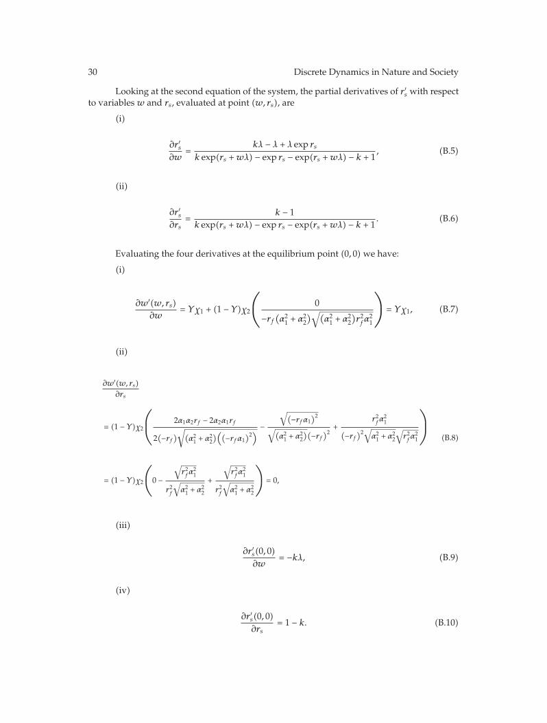
Looking at the second equation of the system, the partial derivatives of r ′s with respectto variables w and rs, evaluated at point (w, rs), are
(i)
∂r ′s∂w
=kλ − λ + λ exp rs
k exp(rs +wλ) − exp rs − exp(rs +wλ) − k + 1, (B.5)
(ii)
∂r ′s∂rs
=k − 1
k exp(rs +wλ) − exp rs − exp(rs +wλ) − k + 1. (B.6)
Evaluating the four derivatives at the equilibrium point (0, 0) we have:
(i)
∂w′(w, rs)∂w
= Yχ1 + (1 − Y )χ2
⎛⎜⎝ 0
−rf(α21 + α2
2
)√(α21 + α2
2
)r2fα21
⎞⎟⎠ = Yχ1, (B.7)
(ii)
∂w′(w, rs)∂rs
= (1 − Y )χ2
⎛⎜⎜⎝
2α1α2rf − 2α2α1rf
2(−rf
)√(α21 + α2
2
)((−rfα1)2)
−
√(−rfα1)2
√(α21 + α2
2
)(−rf)2 +
r2fα21
(−rf)2√
α21 + α2
2
√r2fα21
⎞⎟⎟⎠
= (1 − Y )χ2
⎛⎜⎝0 −
√r2fα21
r2f
√α21 + α2
2
+
√r2fα21
r2f
√α21 + α2
2
⎞⎟⎠ = 0,
(B.8)
(iii)
∂r ′s(0, 0)∂w
= −kλ, (B.9)
(iv)
∂r ′s(0, 0)∂rs
= 1 − k. (B.10)

Discrete Dynamics in Nature and Society 31
So that the Jacobian matrix at point (0, 0) has the following form:
J(0, 0) =
[Yχ1 0
−kλ 1 − k
]. (B.11)
Observe that Jacobianmatrices of the extreme cases, in which all agents are speculatorsor rational, can be easily obtained by the previous calculations simply setting Y = 1 and Y = 0respectively.
C. Contagion Effect: Price in the Case of Contrarian Speculation
In a market only composed by speculators and in the case of χ1 < −1 (strongly contrarianattitude of investors) a two-period cycle appears in the phase plane (w, rs). From an economicpoint of view in this case, the positive excess demand in period t (w∗
3 = −χ1 − 1 ) turns intonegative excess demand in period t + 1 (w∗
4 = χ1 + 1), and correspondingly market pricesoscillate between two values P3 < P < P4.
We can determine the two-period orbit and the exact values of P3 and P4. After twoperiods the system (4.5) becomes
wt+1 = χ21
wt−1(1 + |wt−1|)
(1 +
∣∣χ1(wt−1/(1 + |wt−1|))∣∣)
rs,t+1 = ln
( (exp rs,t−1 + k − 1
)/ exp(rs,t−1 + λwt−1)((
exp rs,t−1 + k − 1)/(exp(rs,t−1 + λwt−1)
) − (k − 1))expλχ1(wt−1/(1 + |wt−1|))
−(k − 1)
)
(C.1)
recalling that Pt = [Pt−1 + k(P − Pt)] expλwt−1, the corresponding price equation is
Pt+1 ={(1 − k)
[kP + (1 − k)Pt−1
]expλwt−1 + kP
}expλχ1
(wt−1
(1 + |wt−1|)), (C.2)
where the expression of Pt+1 has been obtained by a double iteration.The first equation of the system does not depends on rs so, solving in a fixed point we
have two solutions w∗3 = −χ1 − 1 and w∗
4 = χ2 + 1. The corresponding price equation is
P ={(1 − k)
[kP + (1 − k)P
]expλw + kP
}expλχ1
w
(1 + |w|) , (C.3)
giving two different solutions for P depending on w∗3 and w∗
4.When w = w∗
3 = −χ1 − 1
P ={(1 − k)
[kP + (1 − k)P
]expλ
(−χ1 − 1)+ kP
}expλχ1
−χ1 − 11 +
∣∣−χ1 − 1∣∣ , (C.4)

32 Discrete Dynamics in Nature and Society
which simplifies as
P(1 − (1 − k)2
)= kP(1 − k) + kP expλ
(χ1 + 1
), (C.5)
giving the final price P = ((eλ(χ1+1) + 1 − k)/(2 − k))P ≡ P3, corresponding to the expectedreturn (see (2.1)):
r∗s = ln
(1 + (1 − k)
(eλ(χ1+1)
)
eλ(χ1+1) + 1 − k
). (C.6)
P3 is always smaller than P . Indeed P3 < P if (eλ(χ1+1) + (1 − k))/(2 − k) < 1, which simplifiesto λ(χ1 + 1) < 0. This condition is always true under the hypothesis at hand χ1 < −1.
When w = w∗4 = χ1 + 1
P ={(1 − k)
[kP + (1 − k)P
]expλ
(χ1 + 1
)+ kP
}expλχ1
χ1 + 11 +
∣∣χ1 + 1∣∣ , (C.7)
which simplifies to
P(1 − (1 − k)2
)= (1 − k)kP + kP exp−λ(χ1 + 1
). (C.8)
We obtain the solution P = ((e−λ(χ1+1) + (1 − k))/(2 − k))P ≡ P4, corresponding to an expectedreturn:
r∗s = ln
(1 + (1 − k)e−λ(χ1+1)
e−λ(χ1+1) + (1 − k)
). (C.9)
We can observe that P4 is always greater than P . Indeed P4 > P if (e−λ(χ1+1) +1−k)/(2−k) > 1;this inequality is equivalent to λ(χ1 + 1) < 0 which is always satisfied under the hypothesisχ1 < −1.
Acknowledgments
The authors thank the anonymous referees for their suggestions and comments thatimproved the quality of this paper. Thanks are due to Roberto Dieci, Laura Gardini, AnnaAgliari, and Giovanni Zambruno for their careful reading and helpful comments andsuggestions. Any errors are the authors responsibility.
References
[1] C. Chiarella, R. Dieci, and L. Gardini, “The dynamic interaction of speculation and diversification,”Applied Mathematical Finance, vol. 12, no. 1, pp. 17–52, 2005.
[2] E. Bertero and C. Mayer, “Structure and performance: Global interdependence of stock marketsaround the crash of October 1987,” European Economic Review, vol. 34, no. 6, pp. 1150–1180, 1990.
Discrete Dynamics in Nature and Society 33
[3] M. A. King and S. Wadhwani, “Transmission of volatility between stock markets,” The Review ofFinancial Studies, vol. 3, pp. 5–33, 1990.
[4] S. Calvo and C. Reinhart, Capital Flows to Latin America: Is There Evidence of Contagion Effects?MPRAPaper 7124, University Library of Munich, Munich, Germany, 1996.
[5] T. Baig, “Financial market contagion in the Asian crisis,” IMF Staff Papers, vol. 46, no. 2, pp. 167–195,1999.
[6] M. Loretan and W. B. English, “Evaluating correlation breakdowns during periods of marketvolatility,” Board of Governors of the Federal Reserve System International Finance Working Paper658, 2000, http://mpra.ub.uni-muenchen.de/7124/.
[7] G. A. Karolyi and R. M. Stulz, “Why do markets move together? An investigation of U.S.-Japan stockreturn comovements,” Journal of Finance, American Finance Association, vol. 51, no. 3, pp. 951–86, 1996.
[8] F. Longin, “The asymptotic distribution of extreme stock market returns,” Journal of Business, vol. 69,no. 3, pp. 383–408, 1996.
[9] P. Hartmann, S. Straetmans, and C. G. de Vries, “Asset market linkages in crisis periods,” Review ofEconomics and Statistics, vol. 86, no. 1, pp. 313–326, 2004.
[10] K. H. Bae, G. A. Karolyi, and R. M. Stulz, “A new approach to measuring financial contagion,” Reviewof Financial Studies, vol. 16, no. 3, pp. 717–763, 2003.
[11] L. Ramchand and R. Susmel, “Volatility and cross correlation across major stock markets,” Journal ofEmpirical Finance, vol. 5, no. 4, pp. 397–416, 1998.
[12] A. Ang and G. Bekaert, “Regime switches in interest rates,” Journal of Business & Economic Statistics,vol. 20, no. 2, pp. 163–182, 2002.
[13] F. Chesnay and E. Jondeau, “Does correlation between stock returns really increase during turbulentperiods?” Economic Notes, vol. 30, no. 1, pp. 53–80, 2001.
[14] A. Zeevi and R. Mashal, “Beyond correlation: extreme co-movements between financial assets,” 2002,http://ssrn.com/abstract=317122.
[15] R. Rigobon, “Contagion: how to measure It?” NBER Working Papers 8118, National Bureau ofEconomic Research, 2001.
[16] A. Corcos, J. P. Eckmann, A. Malaspinas, Y. Malevergne, and D. Sornette, “Imitation and contrarianbehaviour: hyperbolic bubbles, crashes and chaos,” Quantitative Finance, vol. 2, no. 4, pp. 264–281,2002.
[17] T. Lux, “Herd behavior, bubbles and crashes,” Economic Journal, vol. 105, pp. 881–896, 1995.[18] G. I. Bischi, M. Gallegati, L. Gardini, R. Leombruni, and A. Palestrini, “Herd behavior and
nonfundamental asset price fluctuations in financial markets,” Macroeconomic Dynamics, vol. 10, no.4, pp. 502–528, 2006.
[19] T. Kaizoji, “A synergetic approach to speculative price volatility,” IEICE Transactions on Fundamentalsof Electronics, Communications and Computer Sciences, vol. E82-A, no. 9, pp. 1874–1882, 1999.
[20] A. Tversky and D. Kahneman, “Loss aversion in riskless choice: a reference-dependent model,”Quarterly Journal of Economics, vol. 106, pp. 1039–1061, 1991.
[21] A. Tversky and D. Kahneman, “Advances in prospect theory: cumulative representation ofuncertainty,” Journal of Risk and Uncertainty, vol. 5, no. 4, pp. 297–323, 1992.
[22] J. Cunado, L. A. Gil-Alana, and F. P. de Gracia, “Stock market volatility in US bull and bear markets,”Journal of Money, Investment and Banking, vol. 1, pp. 25–32, 2008.
[23] C. P. Jones, M. D. Walker, and J. W. Wilson, “Analyzing stock market volatility using extreme-daymeasures,” Journal of Financial Research, vol. 27, no. 4, pp. 585–601, 2004.
[24] J. M. Maheu and T. H. McCurdy, “Identifying bull and bear markets in stock returns,” Journal ofBusiness & Economic Statistics, vol. 18, no. 1, pp. 100–112, 2000.
[25] W. F. Sharpe, “Mutual fund performance,” Journal of Business, pp. 119–138, 1966.[26] G. M. Constantinides, M. Harris, and R .M. Stulz, Handbook of the Economics of Finance, vol. 1, Elsevier,
2003.[27] A. Medio and M. Lines, Nonlinear Dynamics, Cambridge University Press, Cambridge, 2001, A prime.