VECTORS of Change in Oceans and Seas Marine Life, Impact

on Economic Sectors

SP1 - Cooperation

Collaborative Project - Large-scale Integrating Project

FP7 – OCEAN - 2010

Project Number: 266445

Deliverable No: 3.1.2 Workpackage: WP3.1

Date: 06/08/13 Contract delivery due date Month 28

Title: Synthesis of evidence for impacts of changes

Lead Partner for Deliverable

University College Dublin

Author(s): T. P. Crowe

Dissemination level (PU=public, RE=restricted, CO=confidential) PU

Report Status (DR = Draft, FI = FINAL) FI

Acknowledgements The research leading to these results has received funding from the European Community’s Seventh Framework Programme (FP7/2007-2013) under Grant Agreement No. [266445] for the project Vectors of Change in Oceans and Seas Marine Life, Impact on Economic Sectors (VECTORS)

D3.2.1 Synthesis of evidence for impacts of changes  

D3.1.2 2 VECTORS

VECTORS Overview

‘VECTORS seeks to develop integrated, multidisciplinary research-based understanding that will contribute the information and knowledge required for addressing forthcoming requirements, policies and regulations across multiple sectors.’ Marine life makes a substantial contribution to the economy and society of Europe. In reflection of this VECTORS is a substantial integrated EU funded project of 38 partner institutes and a budget of €16.33 million. It aims to elucidate the drivers, pressures and vectors that cause change in marine life, the mechanisms by which they do so, the impacts that they have on ecosystem structures and functioning, and on the economics of associated marine sectors and society. VECTORS will particularly focus on causes and consequences of invasive alien species, outbreak forming species, and changes in fish distribution and productivity. New and existing knowledge and insight will be synthesized and integrated to project changes in marine life, ecosystems and economies under future scenarios for adaptation and mitigation in the light of new technologies, fishing strategies and policy needs. VECTORS will evaluate current forms and mechanisms of marine governance in relation to the vectors of change. Based on its findings, VECTORS will provide solutions and tools for relevant stakeholders and policymakers, to be available for use during the lifetime of the project. The project will address a complex array of interests comprising areas of concern for marine life, biodiversity, sectoral interests, regional seas, and academic disciplines and especially the interests of stakeholders. VECTORS will ensure that the links and interactions between all these areas of interest are explored, explained, modeled and communicated effectively to the relevant stakeholders. The VECTORS consortium is extremely experienced and genuinely multidisciplinary. It includes a mixture of natural scientists with knowledge of socio-economic aspects, and social scientists (environmental economists, policy and governance analysts and environmental law specialists) with interests in natural system functioning. VECTORS is therefore fully equipped to deliver the integrated interdisciplinary research required to achieve its objectives with maximal impact in the arenas of science, policy, management and society.

www.marine-vectors.eu

D3.2.1 Synthesis of evidence for impacts of changes  

D3.1.2 3 VECTORS

Contents Overview Report .......................................................................................................................................................... 3

Glossary: Definition of terms used in the following reports ....................................................................................... 10

Appendix 1: What are the effects of macroalgal blooms on the abundance, productivity and biodiversity of marine ecosystems? ................................................................................................................................................. 11

Appendix 2: What are the effects of non-indigenous seaweeds on native benthic assemblages? Variability between trophic levels and influence of background environmental and biological conditions ................... 62

Appendix 3. The diverse effects of marine invasive ecosystem engineers on biodiversity and ecosystem functions .................................................................................................................................................................... 113

Appendix 4: Using higher trophic level modeling to demonstrate the impact of changes in the upper trophic North Sea food web on commercially important fish stocks ................................................................................ 183

Overview Report Executive Summary

Changes in distribution and productivity of species and outbreaks of indigenous or invasive species can cause dramatic changes to the structure and functioning of recipient ecosystems, in terms of biodiversity and ecosystem functioning, with important economic and social consequences.

Three systematic review reports (Task 3.1.1) have been completed, providing quantitative syntheses of current knowledge of effects on biodiversity and ecosystem functioning of (a) outbreaks of macroalgae (b) invasive primary producers (with particular reference to intra- and inter-trophic effects) and (c) invasive ecosystem engineers.

SMS modelling (part of Task 3.1.2) indicated the relative importance of mortality due to fishing and predation for a number of commercial species and demonstrated the potential influence of outbreaks of predatory species.

The outcomes of the systematic reviews and SMS modelling are briefly summarised below and the full reports are available as appendix documents from page 11 onwards.

The findings will help underpin research in WP3.2 to assess impacts of changes in marine ecosystems on their capacity to deliver ecosystem services (WP3.2) and economic benefits to society, now (WP3.3) and in the future (WP5.2). Policy implications will be explored in WP6.

Contrasting findings from the different regional seas will inform region-specific syntheses and models (WP4) and policy responses (WP6).

Introduction Changes in distribution and productivity of species and outbreaks of indigenous or invasive species can cause dramatic changes to the structure and functioning of recipient ecosystems, in terms of biodiversity and ecosystem functioning, with important economic and social consequences (Mack et al. 2000). This deliverable reports on research in WP3.1 to quantify the impact of these changes on ecosystem structure i.e. biodiversity (species richness, identity and relative abundances and physico-chemical parameters) and ecosystem functioning. The findings will help underpin research in WP3.2 to assess impacts of changes in marine ecosystems on their capacity to deliver ecosystem services (WP3.2) and economic benefits to society (WP3.3 and WP5).

D3.2.1 Synthesis of evidence for impacts of changes  

D3.1.2 4 VECTORS

The effects of environmental changes on ecosystem status and dynamics vary considerably depending on the environmental context. Findings from the different regional seas will provide an opportunity to seek general patterns, as well as develop region-specific models (WP4). The deliverable comprises two main components: systematic reviews (Task 3.1.1) and multi-species assessment (SMS) modelling (part of Task 3.1.2). Systematic review is a form of original research that involves formation of a question or hypothesis and testing it by gathering and synthesising existing data enabling increased statistical power through use of advanced meta-analytical techniques. Systematic review follows an established cost-effective methodology which has been developed for biodiversity interventions from a medical model (Collaboration for Environmental Evidence 2013). To realise the full potential of existing data in a policy context and to provide an empirical basis for ecosystem models, we have completed three systematic reviews focussing on impacts on biodiversity and ecosystem functioning of Invasive Alien Species (IAS) and Outbreak Forming Species (OFS) and with particular focus on case study regions (WP4). Each review addresses the impacts of the selected mechanisms on a range of components of biodiversity (benthos, fish, plankton, birds and mammals) and on measures of ecosystem functioning. The applicability of findings across a range of scales and regions was explicitly analysed. The Task was led by the leading authority on environmental systematic review (Pullin, Bangor), with the reviews being undertaken by teams whose expertise spans the focal localities, range of mechanisms and elements of biodiversity and ecosystem functioning. The overall focus and terms of reference for the reviews were informed by consultation with a range of VECTORS researchers (particularly from WPs 2 and 3) and members of the Reference User Group (RUG) and Research Advisory Board (RAB). SMS modelling (Lewy and Vinther 2004) was used to demonstrate how climate and fishery induced changes in the upper North Sea food web influenced the stock trajectories of commercially important fish stocks in the last 30 years. To disentangle effects of natural and anthropogenic pressures it was also analysed whether natural mortality or fishing has contributed most to total mortality. By utilizing SMS hindcasts and predictions the consequences of a strong increase (outbreak) in abundance of an indigenous species - grey gurnard – were analysed for the stock dynamics of commercially important fish stocks. Work from VECTORS WP 2.2 demonstrated that the strong increase in abundance of grey gurnard during the 90s was supported by increasing sea surface temperatures (Kempf et al. 2013) combined with a decrease of predators (e.g., adult cod) and competitors (e.g., juvenile cod) of grey gurnard (Floeter et al. 2005). Results from work in VECTORS WP 1, 2.2 and 3.1 give rise to the assumption that the composition of the prey fields and the spatial overlap between predator and prey types has changed between 1981 and 1991 due to environmental changes. Therefore, stomach input data sets from 1981 and 1991 were utilized in SMS to demonstrate the consequences of altered predator-prey interactions for the stock dynamic of commercially important fish species and the functioning of the upper North Sea food web in general. Finally, the robustness of fishing mortality leading to “Maximum Sustainable Yield” (FMSY) for cod was tested in relation to observed changes in stomach data from 1981 and 1991.

D3.2.1 Synthesis of evidence for impacts of changes  

D3.1.2 5 VECTORS

The SMS modelling work was influenced by WPs 1, 2 and 3. The model itself and the knowledge gained will be used in WP 4.2 and 5.1. More detailed predictions to demonstrate the impact of future changes in spatial predator prey overlap on the productivity of North Sea fish stocks will follow in these WPs. Core Activity Task 3.1.1 Systematic reviews A steering group consisting of lead participants, key stakeholders and CEBC staff met at the outset of the project to review the scope and formulation of each of 3 systematic review questions. The wider VECTORS community was initially consulted at the kick off meeting in Faro. A subsequent workshop was held in London and consultation took place via Skype and email with the wider VECTORS community, particularly members of WP2.1, WP3.2 and 3.3, to clarify how the reviews could best be tailored to benefit VECTORS research. The following systematic review protocols were produced, peer reviewed and subsequently published in the Collaboration for Environmental Evidence Open-Access Journal ‘Environmental Evidence’. They were submitted as part of Deliverable 3.1.1 and can be accessed via the links in the text below:

What are the effects of macroalgal blooms on the structure and functioning of marine ecosystems? A systematic review protocol Devin A Lyons, Rebecca C Mant, Fabio Bulleri, Jonne Kotta, Gil Rilov, Tasman P Crowe Environmental Evidence 2012, 1:7 (29 June 2012)

The effects of exotic seaweeds on native benthic assemblages: variability between trophic levels and influence of background environmental and biological conditions Fabio Bulleri, Rebecca Mant, Lisandro Benedetti-Cecchi, Eva Chatzinikolaou, Tasman Crowe, Jonne Kotta, Devin Lyons, Gil Rilov, Elena Maggi Environmental Evidence 2012, 1:8 (23 July 2012)

How strong is the effect of invasive ecosystem engineers on the distribution patterns of local species, the local and regional biodiversity and ecosystem functions? Gil Rilov, Rebecca Mant, Devin Lyons, Fabio Bulleri, Lisandro Benedetti-Cecchi, Jonne Kotta, Ana M Queirós, Eva Chatzinikolaou, Tasman Crowe, Tamar Guy-Haim Environmental Evidence 2012, 1:10 (6 August 2012)

These protocols formed the basis for systematic searching of the literature and compilation of publications that met the specified criteria for inclusion. Data were extracted from those publications and compiled into spreadsheets for each of the systematic reviews. Those spreadsheets are now online with access restricted to selected researchers within VECTORS at this stage. Meta-analyses were completed to meet the objectives of the reviews. Reports are appended as part of the current Deliverable and findings will be published and widely disseminated. Summaries of key findings are presented below:

What are the effects of macroalgal blooms on the abundance, productivity and biodiversity of marine ecosystems? (for the full report please see Appendix 1)

This work was completed by Devin Lyons, Christos Arvanitidis, Andrew Blight, Eva Chatzinikolaou, Tamar Guy-Haim, Jonne Kotta, Helen Orav-Kotta, Ana M. Queiros, Gil Rilov, Paul J. Somerfield, Tasman P. Crowe

1. Human pressures such as coastal eutrophication, fishing, and habitat degradation have caused macroalgal blooms to increase in frequency and severity. These blooms are often a concern because of their interference with recreation and tourism, and because of health risks. They can also affect the

D3.2.1 Synthesis of evidence for impacts of changes  

D3.1.2 6 VECTORS

structure and functioning of marine and estuarine ecosystems, with potential consequences for other ecosystem services and benefits. We conducted a systematic review and meta-analysis to estimate the effects of macroalgal blooms on seven key measures of ecosystem structure and functioning. In addition to looking at the overall effects of macroalgal blooms, we examined their effects in different marine regions and investigated several ecological and methodological factors that might cause their effects to vary.

2. Overall, macroalgal blooms caused reductions in the abundance of organisms (number (n) = 76 studies) and the number of species (n = 34) where they occurred. They also caused increases in the gross primary productivity of benthic communities (n = 34). Blooms did not have statistically significant effects on the other responses, though it appears that their overall effect on community diversity (Shannon’s index) is likely negative (n = 13).

3. In the Mediterranean Sea, the effects of macroalgal blooms on community abundance (n = 7), species richness (n = 4), and community diversity (Shannon’s Index, n = 3) were consistently more negative than the overall effects. In contrast, blooms had little or no effect on any of these responses in the Northeast Atlantic region (community abundance, n=29; species richness, n = 12; community diversity, n = 2). In the Baltic Sea, the effects tended to be similar to the overall effect (community abundance, n = 16) or more negative (species richness, n = 5; community diversity, n = 5).

4. We identified several factors that contributed to variation in the effects estimated by different studies. The algal taxon responsible for a bloom influenced its effects on community abundance and species richness, possibly because of differences in the complexity and cohesion of the algal mats that they produce. Structurally simple algae such as Ulva, Ulvaria, and Cladophora had negative or neutral effects, while many of the taxa with more complex morphologies had neutral or positive effects.

5. Blooms also had different effects on species richness in different habitats. For example, blooms had a negative effect in unvegetated soft sediment habitats of the subtidal zone, but not in similar intertidal habitats where the potential negative effects of blooms might be offset by the shelter they may provide from temperature and desiccation stress.

6. The method used in studies of benthic productivity and respiration has a strong influence on the observed effects. When the contribution of macroalgal blooms is taken into account, respiration and net primary productivity tend to be higher where blooms occur. However, macroalgal blooms tend to have a negative effect on the functioning of the rest of the community.

7. Work dealing with the causes and consequences of macroalgal blooms tends to emphasize their undesirable, negative effects on marine and estuarine assemblages. Although we find negative overall effects on community abundance and species richness, our results revealed a more complex picture of the impacts of macroalgal blooms. This fuller view of the effects of blooms ought to be taken into account in decisions regarding the management of macroalgal blooms and their drivers. For example, concerns about the negative social and economic effects of macroalgal blooms are often focused on intertidal beaches. Removal of algae from beaches will increase their attractiveness, and reduce the risk of hydrogen sulfide poisoning. However, our results suggest it will have little effect on the abundance of beach fauna, and may even lead to slight reductions in species richness. Thus, if preserving the biodiversity and abundance is an additional objective of bloom management, one may also wish to target rocky intertidal and subtidal soft sediment habitats where the effects of blooms are more severe.

D3.2.1 Synthesis of evidence for impacts of changes  

D3.1.2 7 VECTORS

What are the effects of non-indigenous seaweeds on native benthic assemblages? Variability between trophic levels and influence of background environmental and biological conditions (for the full report please see appendix 2)

This work was completd by Fabio Bulleri, Lisandro Benedetti-Cecchi, Eva Chatzinikolaou, Tasman Crowe , Jonne

Kotta , Devin Lyons, Rebecca Mant, Gil Rilov, Luca Rindi, Elena Maggi

1. In the marine environment, the introduction and spread of non-indigenous benthic macroalgae may cause major alterations to native assemblages and biodiversity.

2. We compared the impacts of non-indigenous seaweeds on native primary consumers (across trophic levels) to those observed on native primary producers (same trophic level). In addition, we assessed variations in the effects of non-indigenous seaweeds on native benthic ecosystems according to the degree of existing human impact (i.e. along a gradient from urban/industrial areas to extra-urban areas to pristine areas).

3. Literature search resulted in the extraction of data from both experimental and observational studies (for a total of 122 papers) investigating the effects of 13 different non-indigenous seaweeds on single species or communities.

4. The effects of non-indigenous seaweeds on native primary producer communities and species were generally negative and greater than those that emerged at higher trophic levels.

5. The effects of non-indigenous seaweeds on most of the response variables examined did not vary among areas characterized by a different degree of human impact. However, the effects on the abundance of consumer species changed from clearly negative when in relatively pristine areas to neutral or slightly positive in areas heavily impacted by human activities. A similar trend emerged for community diversity.

6. A negative impact of non-indigenous seaweeds on native primary producers may result in the lessening of important ecosystem services, such as nutrient cycling, carbon storage, mitigation of coastal erosion through the dampening of wave action, reduced amenity and recreational value of coastal areas.

The diverse effects of marine invasive ecosystem engineers on biodiversity and ecosystem functions (for the full report please see Appendix 3)

This work was completd by Gil Rilov, Devin Lyons, Jonne Kotta, Henn Ojaveer, Ana M. Queirós, Eva Chatzinikolaou, Christos Arvantidis, Serina Como, Paulo Magni, Andrew Blight, Helen Orav-Kotta, Tasman Crowe, Tamar Guy-Haim

1. Invasive ecosystem engineers have great potential to strongly affect native community structure, biodiversity and ecosystem functions.

2. Our analysis revealed highly diverse trends in the overall response of individual species, communities and their function to the presence of invasive ecosystem engineers.

3. The overall (averaged) effect on individual species was small but negative.

4. At the community level, many studies showed a strong effect of the invader on different community attributes, but the overall summary effect was small and non-significant.

D3.2.1 Synthesis of evidence for impacts of changes  

D3.1.2 8 VECTORS

5. In contrast, there was a significant or nearly significant overall strong effect for most ecosystem functions considered. Invasive engineers negatively affected growth and metabolic functions, as well as gross primary production (in sediment and water), and they positively affected nutrient flux and decomposition. Effects on sedimentation were variable and overall non-significant but the number of studies found was very low.

6. In the studies included in the analysis, only a very small number simultaneously quantified invaders’ effects on community/diversity and on ecosystem functions in the same system. Such studies could greatly increase our understanding of how invasive species affect functioning through their effects on biodiversity.

7. Species diversity, richness and evenness were strongly negatively affected in the Mediterranean but showed no trends in other regions. Most of the subgroup analyses could not explain the observed variability in overall impacts, however, indicating that moderators other than those considered here may also play a significant role in the determination of the impact of invasive ecosystem engineers.

8. Based on the patterns revealed in this review, we offer a conceptual framework of the different pathways that may lead to impact on ecosystem function and biological communities by invasive engineer plants and epibenthic sessile invertebrates.

9. Ecosystem services are closely linked to ecosystem functions, so the fact that invasive ecosystem engineers strongly affected many ecosystem functions suggests that ecosystem services may also be affected. This subject deserves further study and analysis, and requires the attention of managers and policy makers.

Part of Task 3.1.2: SMS modelling

Using higher trophic level modeling to demonstrate the impact of changes in the upper trophic North Sea food web on commercially important fish stocks (for the full report please see Appendix 4)

This work was completed by Alexander Kempf (vTI-SF) and Jens Floeter (Uni-HH).

Three Multi Species Assessment Model (SMS) hindcasts were carried out for a range of species to elaborate on the consequences of changes in the diet composition between 1981 and 1991. The first run was the keyrun which used all available stomach data. For the other two runs different sub-sets of stomach data were used to test the sensitivity of results towards stomach input data. The SMS stomach input data were analysed further to detect shifts in the relative stomach contents between commercially important prey species and “Other Food”.

Forecasts were carried out for the period 2011 to 2025 based on the three hindcasts described above. To demonstrate the effect of changes in grey gurnard abundances an additional forecast was carried out in which the abundance of grey gurnard was assumed to decrease to levels before 1991 over the forecast time period. Results were compared to the forecast where the abundance of grey gurnard was assumed to be constant at the level of 2010.

For the scenarios tested, the target F value for cod was increased stepwise from 0.1 to 0.8 to maximize cod catch in the period from 2012 to 2025 when harvesting all other stocks at single species Maximum Sustainable Yield (MSY) targets. The robustness of Fmsy (rate of fishing mortality leading to maximum sustainable yield) for cod was analysed.

D3.2.1 Synthesis of evidence for impacts of changes  

D3.1.2 9 VECTORS

The modelling undertaken showed that:

1. The importance of predation relative to fishing mortality has been increasing in recent years due to a successful reduction in fishing mortality for many stocks in the North Sea. The percentage of natural mortality in total mortality is a useful food web indicator disentangling natural and anthropogenic pressures on fish stocks.

2. Outbreaks of indigenous predators like grey gurnard can have a serious impact on the stock dynamics of commercially important fish species as demonstrated for the interaction between grey gurnard and juvenile cod or whiting.

3. Changes in the diet composition of predators caused by changes in the spatial distribution of prey form an additional mechanism potentially explaining how changes in climate translate into changes in the productivity of fish stocks. The number of years with stomach data available, however, was not enough to differentiate between inter-annual variability and long-term changes.

4. Estimates of FMSY for cod in a multi species context were robust to observed differences between stomach data from 1981 and 1991. Therefore, successful fisheries management based on FMSY seems to be possible despite changes in the upper North Sea food web. However, in a multi species context, trade-offs in yield between different species lead to different options for FMSY. Political decisions are needed in this context.

References Collaboration for Environmental Evidence. 2013. Guidelines for Systematic Review and Evidence Synthesis in Environmental Management. Version 4.2. Environmental Evidence: www.environmentalevidence.org/Authors.htm/Guidelines 4.2.pdf

Floeter, J., Kempf, A., Vinther, M., Schrum, C., Temming, A. 2005. Grey gurnard (Eutrigla gurnadus (L.)) in the North Sea: an emerging key predator? Can J. Fish. Aquat. Sci. 62(8): 1853-1864.

Kempf, A., Stelzenmüller, V., Akimova, A., Floeter, J. 2013. Spatial assessment of predator–prey relationships in the North Sea: the influence of abiotic habitat properties on the spatial overlap between 0-group cod and grey gurnard. Fisheries Oceanography 22(3): 174–192.

Lewy, P., and Vinther, M., 2004. A stochastic age-length-structured multispecies model applied to North Sea stocks. ICES CM 2004/ FF: 20.

D3.2.1 Synthesis of evidence for impacts of changes  

D3.1.2 10 VECTORS

Glossary: Definition of terms used in the following reports: Besc: Biomass that has to be left in the end of the fishing year Blim: limit biomass Bootstrap: a method for assigning measures of accuracy to sample estimates Bpa: precautionary biomass CPUE: Catch per unit of fishing effort F: Fishing mortality rate Fmsy: fishing mortality rate leading to maximum sustainable yield Ftarget: target fishing mortality in e.g., management plans GAMs: statistical models to identify significant non-linear relationships IBTS index: index calculated from the International Bottom Trawl Survey in the North Sea MSEs: tool to evaluate management scenarios MSY: Maximum Sustainable Yield NS: North Sea Ogive: A frequency distribution Q Test: A nonparametric test examining change in a dichotomous variable across more than two observations SMS : Stochastic Multi Species Model SSB : Spawning Stock Biomass

D3.2.1 Synthesis of evidence for impacts of changes  

D3.1.2 11 VECTORS

Appendix 1: What are the effects of macroalgal blooms on the abundance, productivity and biodiversity of marine ecosystems?

Devin Lyons1, Christos Arvanitidis2, Andrew Blight3, Eva Chatzinikolaou2, Tamar Guy-Haim4, Jonne Kotta5, Helen

Orav-Kotta6, Ana M. Queiros7, Gil Rilov8, Paul J. Somerfield9, Tasman P. Crowe10

1 University College Dublin, devin.lyons@ucd.ie 2 Hellenic Centre for Marine Research, arvanitidis@her.hcmr.gr; evachatz@hcmr.gr 3 University of St Andrews, ajb34@st-andrews.ac.uk 4 Israel Oceanographic and Limnological Research, tamar.guy-haim@ocean.org.il 5 Estonian Marine Institute, jonne.kotta@sea.ee 6 Estonian Marine Institute, helen.orav@sea.ee 7 Plymouth Marine Laboratory, anqu@pml.ac.uk 8 Israel Oceanographic and Limnological Research, rilovg@ocean.org.il 9 Plymouth Marine Laboratory, pjso@pml.ac.uk 10 University College Dublin, tasman.crowe@ucd.ie Summary

1. Human pressures such as coastal eutrophication, fishing, and habitat degradation have caused macroalgal blooms to increase in frequency and severity. These blooms are often a concern because of their interference with recreation and tourism, and because of health risks. They can also affect the structure and functioning of marine and estuarine ecosystems, with potential consequences for other ecosystem services and benefits. We conducted a systematic review and meta-analysis to estimate the effects of macroalgal blooms on seven key measures of ecosystem structure and functioning. In addition to looking at the overall effects of macroalgal blooms, we examined their effects in different marine regions and investigated several ecological and methodological factors that might cause their effects to vary.

2. Overall, macroalgal blooms caused reductions in the abundance of organisms (number (n) = 76 studies) and the number of species (n = 34) where they occurred. They also caused increases in the gross primary productivity of benthic communities (n = 34). Blooms did not have statistically significant effects on the other responses, though it appears that their overall effect on community diversity (Shannon’s index) is likely negative (n = 13).

3. In the Mediterranean Sea, the effects of macroalgal blooms on community abundance (n = 7), species richness (n = 4), and community diversity (Shannon’s Index, n = 3) were consistently more negative than the overall effects. In contrast, blooms had little or no effect on any of these responses in the Northeast Atlantic region (community abundance, n=29; species richness, n = 12; community diversity, n = 2). In the Baltic Sea, the effects tended to be similar to the overall effect (community abundance, n = 16) or more negative (species richness, n = 5; community diversity, n = 5).

4. We identified several factors that contributed to variation in the effects estimated by different studies. The algal taxon responsible for a bloom influenced its effects on community abundance and species richness, possibly because of differences in the complexity and cohesion of the algal mats that they produce. Structurally simple algae such as Ulva, Ulvaria, and Cladophora had negative or neutral effects, while many of the taxa with more complex morphologies had neutral or positive effects.

5. Blooms also had different effects on species richness in different habitats. For example, blooms had a negative effect in unvegetated soft sediment habitats of the subtidal zone, but not in similar intertidal

D3.2.1 Synthesis of evidence for impacts of changes  

D3.1.2 12 VECTORS

habitats where the potential negative effects of blooms might be offset by the shelter they may provide from temperature and desiccation stress.

6. The method used in studies of benthic productivity and respiration has a strong influence on the observed effects. When the contribution of macroalgal blooms is taken into account, respiration and net primary productivity tend to be higher where blooms occur. However, macroalgal blooms tend to have a negative effect on the functioning of the rest of the community.

7. Work dealing with the causes and consequences of macroalgal blooms tends to emphasize their undesirable, negative effects on marine and estuarine assemblages. Although we find negative overall effects on community abundance and species richness, our results revealed a more complex picture of the impacts of macroalgal blooms. This fuller view of the effects of blooms ought to be taken into account in decisions regarding the management of macroalgal blooms and their drivers. For example, concerns about the negative social and economic effects of macroalgal blooms are often focused on intertidal beaches. Removal of algae from beaches will increase their attractiveness, and reduce the risk of hydrogen sulfide poisoning. However, our results suggest it will have little effect on the abundance of beach fauna, and may even lead to slight reductions in species richness. Thus, if preserving the biodiversity and abundance is an additional objective of bloom management, one may also wish to target rocky intertidal and subtidal soft sediment habitats where the effects of blooms are more severe.

Background Marine and estuarine ecosystems are under pressure from a wide variety of anthropogenic stressors, which have degraded their environmental quality (Lotze et al. 2006, Halpern et al. 2008). This ongoing degradation is commonly believed to have contributed to an increase in the frequency, magnitude, and extent of ‘species outbreaks’, or episodic explosions in the populations of taxa that are normally a less abundant component of the local community. Macroalgal blooms provide a striking example of this phenomenon. Macroalgal blooms are outbreaks of opportunistic seaweeds, which may form dense canopies or large mats of drifting algae. These blooms inhibit recreation, diminish aesthetic enjoyment of the coastal zone, interfere with tourism, fishing and mariculture, and pose a potential risk to human health when toxic gases are emitted from rotting macroalgae (Charlier & Lonhienne 1996, Dion & Le Bozec 1996, De Leo et al. 2002, Chrisafis 2009, Samuel 2011). They also have a variety of ecological effects on marine and estuarine ecosystems. They alter the physical and chemical environment, compete with other primary producers, interfere with the feeding of birds and fish, and have demonstrated impacts on populations of many invertebrate species (Fletcher 1996, Raffaelli et al. 1998). These negative social, economic, and ecological effects have caused considerable concern and prompted costly algal removal programs in some affected areas (Morand & Merceron 2005). Coastal eutrophication and reductions in herbivore populations caused by fishing and habitat degradation are the two primary drivers of macroalgal blooms (Teichberg et al 2012). Expanding human population, fertilizer use, livestock waste production, and fossil fuel combustion have overcome the nitrogen and phosphorus limitation of coastal and estuarine waters, leading to accelerated macroalgal nutrient uptake, faster macroalgal growth, and more frequent macroalgal blooms around the world (Nixon 1995, Conley 1999, Howarth 2008, Teichberg et al. 2010). Loss of herbivores has aggravated the problems caused by eutrophication. For example, harvesting of large predatory fish in the Baltic Sea has increased macroalgal abundance via a trophic cascade. With reduced predatory pressure of large fish, the abundance of smaller predators has increased, driving down populations of invertebrate grazers, and allowing macroalgae to proliferate (Eriksson et al. 2009, Sieben et al. 2011). The combined effects of eutrophication and reduced herbivore populations on macroalgal blooms may be larger than one would expect. A recent meta-analysis found that, while each of these factors increases macroalgal biomass on their own, they also interact synergistically to enhance it even further (Burkepile & Hay 2006). Once macroalgal blooms develop, they have a direct impact on a wide variety of marine and estuarine taxa. For example, when mats of blooming macroalgae settle on the seafloor, they can reduce the diversity and abundance

D3.2.1 Synthesis of evidence for impacts of changes  

D3.1.2 13 VECTORS

of animal assemblages by inducing hypoxia and releasing hydrogen sulfide from the sediments (Gamenick et al. 1996, Wetzel et al. 2002). These changes to the sedimentary environment can therefore act as sources of physiological stress to benthic fauna. Repositioning of mobile burrowers towards the sediment-water interface is typically observed as an avoidance behavior (Wright et al. 2010), impacting important sedimentary ecosystem processes that these species mediate (Gribben et al. 2009, Queirós et al. 2011). The competitive effects of macroalgal blooms have been implicated in the world-wide decline in seagrass beds (Valiela et al. 1997, McGlathery 2001), and linked to local declines in non-blooming algae (Kautsky et al. 1986, Worm et al. 1999). By driving declines in such foundation species, macroalgal blooms may also have negative indirect effects on other members of the biological community. A number of effects of macroalgal blooms are also positive and may be considered beneficial. For example, macroalgal blooms increase the transfer of nutrients from the water column to the sediments and other macroalgae, thereby reducing nutrient levels in eutrophic waters (Thybo-Christesen et al. 1993, Hardison et al. 2010). Accumulations of macroalgae can also increase habitat complexity, enhance dispersal of other species, and provide animals with food and shelter (Wilson et al. 1990, Holmquist 1994, Holmquist 1997). As a result, macroalgal blooms may actually enhance, rather than reduce, biodiversity and secondary production in some ecosystems (Holmquist 1997, Dolbeth et al. 2003, Bolam & Fernandes 2002). Objective of the Review Given their opposing positive and negative influences on marine and estuarine ecosystems, understanding the overall effects of macroalgal blooms and why they vary is an important challenge. Several qualitative reviews on the drivers and ecological impacts of macroalgal blooms have been published in the past (e.g. Fletcher 1996, Raffaelli et al. 1998). Here we provide a quantitative synthesis that complements these reviews by estimating the net impact of their positive and negative effects on seven key measures of ecosystem structure and functioning using meta-analysis. Specifically, our primary research question is: What are the effects of macroalgal on species richness, community diversity (Shannon Index), community evenness (Pielou Index), community-level abundance (biomass, density, cover), gross primary productivity, net primary productivity, and community respiration?

In assessing these effects we will also address the following secondary questions:

1. Do macroalgal blooms have different effects in different regions? 2. Do blooms of different algal species have different effects? 3. How do the effects of macroalgal blooms vary among different habitat types? 4. Do different types of community (e.g. algal communities, invertebrate communities, fish communities)

respond differently to macroalgal blooms? 5. How do the methods used to study macroalgal blooms (study setting, type of study, choice of response

variable, measurement methods) affect the observed effects? Methods We carried out this synthesis using the process of systematic review, following guidelines recommended by the Collaboration for Environmental Evidence (2013). Our peer-reviewed protocol for conducting this review is available in a separate publication (Lyons et al. 2012). Below we provide a brief description of our methods, and note a number of amendments made to the protocol during the review process. Search Strategy and Study Inclusion Criteria Using two sets of search terms, we searched for studies that could be used to evaluate the effects of macroalgal blooms and macroalgal mats on the structure and functioning of marine and estuarine ecosystems. This search was conducted on 28 June 2012 using the Web of Science and Scopus online databases. The first set of search

D3.2.1 Synthesis of evidence for impacts of changes  

D3.1.2 14 VECTORS

terms was intended to identify studies examining blooms of macroalgae. It included terms for algal taxa known to undergo blooms, as well as general terms describing macroalgal blooms and other accumulations of macroalgae or macroalgal detritus (Annex A). This set of terms was combined with a second set of terms intended to capture a broad range of macroalgal blooms’ potential effects on the structure and functioning of marine and estuarine ecosystems (Annex A). The references returned by this search were evaluated for inclusion in our study using a three-stage screening process. This screening process aimed to identify the studies that were relevant to our review questions, while removing studies that did not contain relevant data. At each stage, studies were evaluated according to inclusion criteria described below. We began by assessing the titles to remove any spurious references that dealt with completely unrelated topics. Following this initial assessment, we evaluated the abstracts of the remaining references. Finally, we assessed the full text of the studies that had been retained. If, at any stage, it was unclear whether or not a study met our criteria, it was retained for assessment at the following stage.. One reviewer carried out the initial assessment of the titles. Several reviewers carried out the second and third stages of the assessment. In order to clarify the inclusion criteria and ensure their consistent application, two samples of the abstracts were assessed by all of the reviewers before the references were divided among them. We assessed consistency among reviewers with a multi-rater Kappa statistic, using a Kappa of at least 0.5 to indicate an acceptable degree of consistency. The assessment of the first sample of 60 abstracts was not sufficiently consistent (Kappa = 0.27). We discussed inconsistent assessments and application of the inclusion criteria, resulting in increased consistency in the assessment of the second sample of 20 abstracts (Kappa = 0.57). Although this second assessment was considered sufficiently consistent, we discussed any inconsistent assessments in order to further clarify the inclusion criteria. To be retained when the title and abstract were assessed, the study had to meet four criteria. First, it had to report on the results of a manipulative experiment or an observational study, carried out in the field or in a laboratory setting. We did not include studies that reported results derived from theoretical models. Second, it had to examine an ecosystem or an ecosystem component affected by marine or brackish-water macroalgal blooms. This included, but was not limited to: a) coastal, estuarine, and lagoonal ecosystems, b) benthic, demersal and pelagic ecosystem components, c) plants, fish, birds, invertebrates, algae, microbes. We wished to focus on temperate and sub-tropical ecosystems so we did not include studies conducted in coral reefs. Third, it had to involve a comparison between an affected state (with macroalgal blooms or mat of macroalgae) and a control state (without macroalgal algal bloom or mats of macroalgae). This included both spatial and temporal comparisons. Fourth, it had to report on a measure of ecosystem structure or functioning. For example, we included studies measuring the effects of macroalgal blooms on the abundance of organisms, the number or diversity of species, and ecosystem productivity. We used three additional criteria that were not explicitly stated in the original protocol (Lyons et al. 2012) when studies were assessed at full text. First, we elected to focus on those that reported one or more of the following seven specific outcomes: 1. species richness, 2. community diversity (Shannon index), 3. community evenness (Pielou Index), and community-level measures of 4. gross primary productivity, 5. net primary productivity, 6. respiration, and 7. biomass, density, or cover (“community abundance” hereafter). We selected these variables because we considered them to be among the most important community-level variables and because our initial assessments suggested that they would be represented in the study set. We also searched for data on community-level measures of secondary production, but failed to find any appropriate studies. Second, we only retained studies that provided sufficient information so that an effect size (Hedges’ g) could be calculated (generally means, sample sizes and standard deviations or standard errors). When incomplete information was available, we attempted to obtain the missing information from the authors of the study. If it was not forthcoming, we excluded the study from the review and meta-analysis. Third, when a study used experiments, we only

D3.2.1 Synthesis of evidence for impacts of changes  

D3.1.2 15 VECTORS

included experiments where algal abundance was directly manipulated, including factorial experiments where algal abundance and other factors were manipulated simultaneously. We found several studies where manipulations of other factors (e.g. nutrients, grazer abundance) resulted in macroalgal blooms, but algal abundance was not directly manipulated. We decided to exclude these studies because the any effects of macroalgal blooms in these studies are irrevocably confounded with those of the manipulated factor. We discovered several instances where more than one reference reported on the same study (i.e. they made exactly the same comparison using exactly the same data). In order to avoid including the same effect more than once, we either chose the study that presented the data for the comparison most fully and clearly, or we randomly selected one study and excluded the other. Study Quality Assessment, Data Extraction and Effect Size Calculation The quality of studies that met our criteria for inclusion was assessed according to their susceptibility to bias and the appropriateness of the study design to evaluate the effects of macroalgal blooms at the ecosystem scale. To assess study quality, we classified studies according to the following characteristics:

a) Study setting – i) lab or ii) field b) Study type – i) manipulative experiment or ii) observational c) Appropriateness of controls- - i) appropriate ii) inappropriate iii) unclear d) Allocation of replicates – i) randomization ii) haphazard iii) other e) Replication appropriateness - i) appropriate ii) inappropriate iii) unclear f) Size of replicates – i) bay/bloom scale or larger ii)> 1 m2 iii)< 1 m2 g) Study extent – i) multiple blooms ii) full bloom iii) sub-bloom h) Confounding factors - i) present ii) not present iii) unclear

Replicate and control appropriateness assessments involved subjective judgments. We considered whether individual replicates appeared to be spatially and temporally independent of one another, whether affected areas appeared to be independent of control areas, and control replicates were sufficiently similar to affected areas to serve as appropriate controls. When possible, means, standard errors, standard deviations and sample sizes were extracted directly from tables and the text of the articles. In other cases, data were extracted from figures using ImageJ (Schneider et al. 2012), DataThief III (Tummers 2006), or Engauge Digitizer (Mitchell 2010) software. In addition to data on the outcome variables, we recorded the geographic coordinates and region where the study was conducted. In European waters we used the marine regions defined in the Marine Strategy Framework Directive (European Union 2008). Elsewhere, we used the large marine ecosystems defined by Sherman & Hempel (2008). We also recorded when the study was conducted, replicate size and other characteristics of the study, including information on a number of variables that might modify the effects of macroalgal blooms (described below). The extracted data were used to calculate an effect size for each study. We chose to use Hedges’ g as our effect size metric. Hedges’ g is the bias-corrected mean difference in the response variable between the ‘treatment’ (i.e. algal bloom) and control conditions, standardized by the within-group standard deviation. It is calculated using the following formula:

1

34 9

where is the mean for the algal treatment, is the mean for the control, is the within-groups standard deviation pooled across groups, and df is the degrees of freedom used to calculate . The variance of g is calculated as:

D3.2.1 Synthesis of evidence for impacts of changes  

D3.1.2 16 VECTORS

21

34 9

where is the sample size for the algal treatment and is the sample size for the control. The equations above are for studies with independent groups. For studies with paired groups we used the adjusted equations given in Borenstien et al. (2009). For studies with before-after-control-impact (BACI) designs, and similar designs, we calculated the effect size and variance following Morris (2008). In calculating the variance for BACI studies, it is necessary to know, or estimate, the intraclass correlation. Repeated measures taken from the same replicate are likely to be positively correlated. Thus, the intraclass correlation for repeated measures is likely to fall between 0 and 1. When the data presented in the article were insufficient to estimate it directly, we assumed an intraclass correlation of 0.5. This produces a variance estimate that is larger than if we assumed the ‘before’ and ‘after’ were completely independent, and smaller than if we assumed they were perfectly correlated. It does not affect the estimate of the effect size. Preliminary analyses suggested that, although the intraclass correlation affected the variance estimate for individual studies, it had little effect on our overall analysis. This is likely due to the fact that the effect sizes of our studies were highly heterogeneous (see results), and the fact that we are using random effects meta-analyses. When studies are heterogeneous, random effects models use more balanced study weights than fixed effects analyses, and are less influenced by differences in effect size variance or sample size (Borenstien et al. 2009). Some references contained data for more than one outcome, or more than one result for the same outcome. Data for each of the seven outcomes were analysed in separate meta-analyses, and were therefore treated as independent studies. Multiple results for the same outcome were handled according to the nature of the data. When the results of multiple studies were presented (e.g. multiple independent experiments, or one experiment and one observational study), we calculated a separate effect size for each study and treated them as independent. Similarly, when an experiment was repeated at several sites (separated by at least 1 km), we calculated separate effect sizes for each site. We considered it appropriate to treat individual studies or sites equally, regardless of whether their results were compiled and published in one article, or spread over several articles. When studies reported repeated measurements from the same experimental replicates, we used data from the last sampling date to estimate effect sizes. This provided us with the best estimate of blooms’ long-term effects and allowed us to avoid using many non-independent estimates. Our database included studies where the macroalgal treatment was crossed with other factors, and studies with results for multiple levels of macroalgal treatment. When the macroalgal treatment was crossed with another factor, we first calculated separate effect sizes at each level of the other factor. Because these estimates arise from independent replicates we calculated the overall effect size for the study using a fixed effects meta-analysis (Borenstien et al. 2009). When two or more levels of macroalgal treatment shared a common control, their effect sizes cannot be considered independent. In such cases, we calculated the overall effect size as the average of the two effects and estimated the variance as:

1√ √

where m is the number of non-independent responses, rij is the correlation between effect size j and effect size k, which is equal to 0.5 for if the sample sizes of all treatment levels is equal (Borenstien et al. 2009), Vj is the variance for effect size j and Vk is the variance for effect size k.

D3.2.1 Synthesis of evidence for impacts of changes  

D3.1.2 17 VECTORS

Rather than reporting overall community abundance, species richness, diversity, and evenness, most studies broke these responses down by smaller taxonomic or functional groups. As described below, we examined differences in macroalgal blooms’ effects on invertebrates, fish, birds, microalgae, non-blooming macroalgae, seagrasses, and bacteria. To do so, we calculated separate effect sizes for each of these taxonomic groups, that is we treated results for these taxonomic groups as separate studies. When a study reported results on these taxonomic groups at multiple hierarchical levels of organization, we used the most aggregated data. For example, if a study presented invertebrate biomass as well as separate values for mollusks, crustaceans, and echinoderms, we used invertebrate biomass. When data from multiple non-overlapping subgroups was presented (e.g. infaunal and epifauna invertebrates), we calculated the overall effect size as the mean of their individual effect sizes, and calculated the variance using the same equation we used for treatment levels sharing a common control. This required us to estimate the intraclass correlation (rij) for each pair of outcomes. Correlations in the abundance, richness, diversity, and evenness of different taxonomic or functional groups can fall anywhere between -1 and 1. Thus, when data allowing the estimation of intraclass correlation were not available, we assumed that the intraclass correlation fell at the midpoint of this range (0). This produces variance estimates that are larger than if we were to assume that the outcomes were negatively correlated, and smaller than if we were to assume that the outcomes were positively correlated. The intraclass correlation is not used to calculate individual estimates of the effect size, so these estimates are not influenced by this assumption. If a study presented multiple measures of community abundance (e.g. invertebrate biomass and invertebrate density), we only used one of these measures. Whenever possible we extracted data for the biomass of organisms per unit area. If such data were not available we extracted data for density or percentage cover. Meta-Analysis We synthesized the data for the effects of macroalgal blooms on each of our seven outcomes of interest using random effects and mixed effects meta-analyses. We conducted these in R (R Development Core Team 2012), using the package ‘metafor’ (Viechtbauer 2010), and the DerSimonian–Laird estimator (DerSimonian & Laird 1986). We began by conducting overall analyses using random effects models. We used funnel plots and a rank correlation test for funnel plot asymmetry to assess whether there was any evidence of potential publication bias, or other small study effects. To estimate the effect of macroalgal blooms in different regions, we conducted mixed effect meta-analysis, using region as a fixed factor. We used random effects and mixed effects models rather than fixed effects models because we assume that the true effects of macroalgal blooms vary in different ecological contexts. Random effects and mixed-effects models were therefore deemed as suitable approaches because they can be used to account for this heterogeneity, and for sampling error (Borenstien et al. 2009). As a result, the estimated summary effects have wider confidence intervals than those estimated using fixed-effects models. Potential Effect Modifiers We were interested in investigating the potential influence of both ecological and methodological factors that might influence the effects estimated by each study. When the overall meta-analysis found statistically significant heterogeneity in the effects estimated by different studies, we used mixed model meta-analyses to conduct subgroup analyses investigating these potential ‘effect modifiers’. The importance of each modifier variable was examined in a separate analysis, using the potential effect modifier as a fixed effect. We conducted four subgroup analyses for all of the outcomes that had sufficient data (i.e. data from studies falling into more than one subgroup per analysis). These examined the potential influence of algal identity, habitat, study type, and study setting on the observed effects. To examine the effect of algal identity we grouped studies according to the Genus of the algae responsible for the bloom. For the habitat analysis we assigned each study to one of eight habitat categories: rocky intertidal, rocky subtidal, subtidal seagrass bed, intertidal seagrass bed, oyster reef, intertidal sand/mud, subtidal sand/mud, and pelagic habitats). The study type analysis investigated whether there were differences between the effects observed in experiments and observational studies, and the study setting analysis compared field studies and lab studies.

D3.2.1 Synthesis of evidence for impacts of changes  

D3.1.2 18 VECTORS

We conducted three additional subgroup analyses that were specific to particular response variables. First, we conducted an analysis to determine whether there was a difference between studies that used biomass, density, or cover as their measure of community abundance. Second, because taxa are likely to differ in their responses to macroalgal blooms, we also compared the effects of macroalgal blooms on different types of community (invertebrates, fish, microalgae, non-blooming macroalgae, seagrasses, bacteria, and mixed assemblages). This sub-group analysis was conducted for the community abundance, species richness, community diversity, and community evenness outcomes. Third, we compared studies, which used two different classes of methods to measure benthic productivity and respiration. The first used methods that included the contribution of the bloom’s respiration or productivity in their estimates. The second measured only the effect of the macroalgal bloom on the productivity or respiration of the community. Given that macroalgal blooms often occur in response to increased nutrient loads, and are highly productive under those conditions (Fletcher 1996), we expected that the blooms would increase productivity and respiration when their contribution was taken into account. We expected that blooms would have a negative effect on the productivity and respiration of communities under the macroalgal mat due to their competitive influence, and their effects on sediment chemistry (Gamenick et al. 1996, Wetzel et al. 2002). Results

Our bibliographic search returned 906 references, 638 of which were retained following the initial screening of the titles. We retained 298 references after the abstracts had been assessed. When we assessed the full text of those references, we found 52 that contained relevant studies. Many studies of macroalgal blooms were excluded because they did not include relevant comparisons to controls, or because they did not provide sufficient data to calculate effect sizes. Many others were excluded because they examined the productivity or abundance of single species, rather than community or ecosystem-level responses to algal blooms. The majority of the references we retained contained data for more than one outcome, or multiple estimates for a single outcome. In all, we were able to calculate effect size estimates for 153 studies. These studies came from the coasts of all continents, except Antarctica, but more than 70% of them were conducted in European waters (Figure 1). The datasets tended to be biased towards studies of ephemeral green algae, of soft sediment habitats, and of invertebrate communities. Below we provide a detailed description of the data for each outcome, along with its results. Community Abundance We found 76 studies of macroalgal blooms’ effects on community abundance in 42 different references (Figure 2). These were distributed among 13 different marine regions around the world, but were most concentrated in the northeast Atlantic, Baltic Sea, and Mediterranean Sea (Figures 1A, 3). Over half of the studies examined the effects of ephemeral green algae such as Ulva (including those formerly known as Enteromorpha), Ulvaria, and Cladophora, and studies of mixed blooms were also common (Figure 4A). Research in soft sediment habitats (seagrass beds, subtidal sand/mud habitats, and intertidal sand/mud) was well represented in the dataset, but there were relatively few studies of hard bottom and pelagic habitats (Figure 4B). The majority examined the responses of benthic invertebrate communities (45 studies), and the responses of microalgae were also well represented (16 studies). Three studies reported effects on the abundance of mixtures of invertebrates and macroalgae. The effects of macroalgal blooms on communities of fish, bacteria, seagrasses, and other macroalgae were not well documented (Figure 4C). Thirty-one effect size estimates came from observational field studies and 45 came from experiments (18 lab, 27 field). On average, macroalgal blooms had a negative effect on the abundance of organisms in marine and estuarine communities (Hedges’ g ± 95 % C.I. = -0.49 ± 0.34). Although the overall effect was negative, the impacts observed in individual studies were heterogeneous, ranging from strong negative to strong positive effects (Figure 2, Table 1). Neither regional differences nor the potential effect modifiers fully accounted for this heterogeneity, though two of the mixed model analyses did find significant differences between subgroups. First, the regional

D3.2.1 Synthesis of evidence for impacts of changes  

D3.1.2 19 VECTORS

analysis indicated that the effects of macroalgal blooms varied significantly between marine regions (Table 1, Figure 3). The overall effect was negative in all regions except the southwest Australian shelf and the Gulf of Mexico. However, only the negative effects in the Mediterranean Sea, Humboldt Current, and California Current regions were statistically significant (Figure 3). Second, the identity of the macroalgal species had a significant influence on blooms’ effects (Table 1). Ulvaria and Cladophora had significant negative effects on community abundance, while Vaucheria had a positive effect (Figure 4A). However, none of these effects were based on more than four studies. The well-studied effects of Ulva and mixed algae were very similar to the overall mean effect, but their confidence intervals overlapped with zero, as did those of the other algal groups. None of the other factors significantly influenced the effects on community abundance. However, the mixed models did reveal a number of interesting patterns. Macroalgal blooms reduced community abundance in all habitats, though only the confidence intervals for rocky intertidal and subtidal soft sediment habitats excluded zero (Figure 4B). There was essentially no effect of blooms on bacterial abundance in the one study where it was examined (Figure 4C). The abundance of seagrasses, mixed assemblages, microalgae, other macroalgae, invertebrates, and fish were lower where blooms were present. However, this difference was only statistically significant for the numerically dominant studies of invertebrate communities. The subgroups of all three methodological factors (abundance measurement, study type, and study setting) consistently produced negative effect size estimates (Figure 4 D-F). Species Richness Our search for studies investigating the effects of macroalgal blooms on the number of species yielded 34 effect size estimates, arising from 24 different references (Figure 5). These studies were conducted in 11 different marine regions (Figures 1, 6A). As with community abundance, research effort was concentrated in European waters, with 21 studies coming from the northeast Atlantic, Baltic Sea and Mediterranean Sea (Figure 6A). There were also four studies from the Northeast U.S. Continental Shelf, and a few studies from seven other marine regions. Studies examining effects of Ulva and mixtures of algae made up the bulk of our dataset (15 and 10 studies, respectively), but we also found a few studies of Vaucheria, Laurencia, Gracilaria, Fucus, and Cladophora (Figure 6B). The dataset spanned all of the benthic habitats but did not include any pelagic studies. As with community abundance, studies from intertidal and subtidal soft sediment habitats were numerically dominant. While a few studies examined macroalgal assemblages, fish assemblages, bird assemblages, or mixed assemblages, most studies examined the richness of invertebrate assemblages (25) (Figure 6C). The dataset included 19 experiments and 15 observational studies. All but one of the 34 studies was conducted in the field. Our overall analysis revealed that macroalgal blooms caused a reduction in species richness (Hedges’ g ± 95 % C.I. = -0.64 ± 0.48), but the effects of individual studies were highly heterogeneous (Figure 5, Table 2). None of our subgroup analyses fully accounted for this heterogeneity. There were some differences in the effects observed in different marine regions (Figure 6A, Table 2). Blooms appeared to have very little effect in the Northeast Atlantic marine region, but the effects were clearly negative in both the Baltic and Mediterranean Seas. The largest difference was between the Humboldt Current and the Gulf of Mexico regions, which found very large negative and positive effects, respectively. However, each of these estimates was based on the results of only a single study. The identity of the macroalgal species, and the type of affected habitat modified the effects of macroalgal blooms on species richness (Figure 6B-C, Table 2). Cladophora had a strong negative effect on species richness, and algal mixtures had an effect very similar to that observed in the overall analysis. Single studies of Vaucheria and Laurencia suggested that these species have positive effects. The effects of other algal groups were subtler, and their confidence overlapped with zero. Similar to the results for community abundance, the strongest effects of macroalgal blooms were observed in subtidal soft sediment habitats and in the single study conducted in the rocky

D3.2.1 Synthesis of evidence for impacts of changes  

D3.1.2 20 VECTORS

intertidal. Effects in both these habitats were negative, as were the non-significant effects in oyster reefs and the rocky subtidal. The mean effects in subtidal seagrass beds and intertidal soft sediments were slightly positive, but their confidence intervals included zero. Macroalgal blooms significantly reduced the richness of only invertebrate communities, but overall there was no significant difference between the effects of blooms on different community types (Figure 6D, Table 2). Similarly, there was no difference in the effects of macroalgal blooms between different study types or settings (Figure 6E-F, Table 2). Community Diversity (Shannon’s Index) We were able to find 13 relevant studies of the effects of macroalgal blooms on the diversity of marine and estuarine ecosystems (as measured by Shannon’s index) in 10 different references (Figure 7). Ten of the studies were conducted in European waters, five in the Baltic Sea, three in the Mediterranean Sea, and two in the Northeast Atlantic. The additional three studies came from the Yellow Sea, the Southwest Australian Shelf, and the Patagonian Shelf. The algal groups represented in this dataset included Ulva, Gracilaria, Fucus, Cladophora, and mixtures of algal species (Figure 8B). Again, studies which examined the effects of blooms in soft sediment habitats were more numerous, with only one study from another habitat (Figure 8C). Eleven of the studies investigated the diversity of invertebrate assemblages. The other two studies examined the response of a bacterial community and a mixed assemblage of invertebrates and algae. All of the studies were conducted in the field. Five were experiments and eight were observational studies. Overall, the presence of macroalgal blooms caused a reduction in the diversity of marine and estuarine communities (Hedges’ g ± 95 % C.I. = -0.92 ± 0.95), however the confidence interval for this effect overlapped slightly with zero, and was not statistically significant (Figure 7, Table 3). Although the effect sizes for different subgroups varied slightly, neither the regional analysis nor the analyses for the effects of algal group, habitat, community type, or study type revealed significant differences between different subgroups (Figure 8, Table 3). The subgroup analyses did reveal that the negative effects of macroalgal blooms in subtidal soft sediment habitats, and the negative effects experienced by invertebrate communities were statistically significant (Figure 8C-D). Thus it appears that the non-significance of the overall result was driven by the marginally positive effects observed in the small number of studies conducted in different habitats, and/or examining different types of community. Community Evenness (Pielou’s Index) Our dataset included information from seven relevant studies of community evenness, comprising five experiments and two observational studies from six different publications (Figure 9). One study examined an Ulva bloom, three examined algal mixtures, one examined the effects of Gracilaria, and two examined mats of Fucus. Aside from one study from the southwest Australian shelf, the remainders were European, with five from the Baltic Sea and one from the Northeast Atlantic. Five of the studies were carried out in subtidal soft sediment habitats, with one each from an intertidal soft sediment habitat and a subtidal seagrass bed. All of these examined the evenness of invertebrate communities in the field. We found that macroalgal blooms had very little effect on community evenness, overall (Hedges’ g ± 95 % C.I. = -0.08 ± 1.07). The individual effects were heterogeneous among studies, including positive and negative effects (Figure 9, Table 4). However, neither the regional analysis, nor potential effect modifiers we examined (algal identity, habitat type, study type) explained any of this heterogeneity (Figure 10, Table 4). Gross Primary Productivity We found six studies of the effects of macroalgal blooms on gross primary productivity in four different references (Figure 11). All of these studies were conducted in the Northeast Atlantic marine region and measured benthic

D3.2.1 Synthesis of evidence for impacts of changes  

D3.1.2 21 VECTORS

productivity using methods that included productivity of the algal mat in their estimates. As a consequence, we did not conduct a regional analysis or a subgroup analysis for measurement methods. Four studies focused on blooms of Ulva, one focused on algal mixtures, and one examined the effect of Gracilaria. The studies were conducted in three habitat types: subtidal soft sediments (two), an intertidal seagrass bed (one), and intertidal soft sediments (three). Five studies were experimental and one was observational. One half of the studies were carried out in the lab, the other in the field. Our overall meta-analysis indicated that macroalgal blooms have a strong positive effect on gross primary productivity (Hedges’ g ± 95 % C.I. = 2.6 ± 1.4). Although all of the individual studies found positive effects, these effects were heterogeneous (Figure 11, Table 5). The currently available evidence does not offer any convincing explanation for this heterogeneity. The regional analysis and the subgroup analyses for the effects of algal identity, habitat type, study type, and study setting all did not show statistically significant differences between different subgroups (Figure 12, Table 5). Net Primary Productivity We found eight relevant studies investigating the effects of macroalgal blooms on net primary productivity in seven different references (Figure 13). Six of these came from the Northeast Atlantic, with one study from the Baltic Sea, and one study from the East-Central Australian Shelf making up the rest of the dataset. Five of the studies focused on blooms of Ulva, one focused on Gracilaria, one focused on Cladophora, and one focused on a mixture of algae. All of the studies examined benthic productivity, in subtidal and intertidal seagrass and soft sediment habitats (Figure 14C). Five of the studies (four observational, one experiment) measured productivity using methods that included the contribution of the mat in their estimates, and the other three (all experimental) used measurements that did not. Overall, the presence of macroalgal blooms caused a slight increase in net primary productivity (Hedges’ g ± 95 % C.I. = 0.4 ± 2.1), however this effect was not statistically significant and its’ confidence interval was very wide (Figure 13, Table 6). The mixed-model meta-analyses suggested that there were no differences between regions or algal groups in their overall effects, and that none of the individual subgroup effects were statistically significant (Figure 14A-B, Table 6). This was not the case for the effects of habitat, measurement methods, study type, and study setting. Overall, macroalgal blooms strongly increased net primary productivity in the three subtidal soft sediment habitat studies, and strongly decreased net primary productivity in the two intertidal soft sediment studies, driving a significant habitat effect in the mixed model (Figure 14C, Table 6). The smaller effects observed in subtidal and intertidal seagrass beds had confidence intervals that overlapped with zero, indicating that they were not statistically significant. Our prediction that different measurement methods would produce opposing effects was borne-out by the data. Studies with measurements that included the productivity of the algal mat in their estimates found that macroalgal blooms had a large, positive effect on net primary productivity, while those that excluded the contribution of the bloom from their estimates found a large negative effect (Figure 14D). In addition, the test of study heterogeneity was non-significant when measurement methods were taken into account, suggesting this factor explains the heterogeneity observed in the full dataset (Table 6). The subgroup analyses for the effects of study type and study setting found significant differences between the results for experiments and observational studies, and between studies conducted in the field and in the lab (Table 6). Overall, observational studies found that blooms increased net primary productivity and experimental studies found that blooms decreased net primary productivity, though the confidence interval for the experimental studies did overlap with zero (Figure 8E). The overall estimate for field studies was large and negative, but it was based on the results of a single study (Figure 14F). A smaller positive effect was estimated from the seven lab studies, but this effect was not statistically significant. However, both study type and study setting were partially confounded with the methods used to measure productivity.

D3.2.1 Synthesis of evidence for impacts of changes  

D3.1.2 22 VECTORS

Respiration We found nine relevant studies of benthic community respiration in eight different references (Figure 15). Seven of these studies were conducted in the Northeast Atlantic region, with the other two studies coming from the Scotian Shelf and the East-Central Australian Shelf. Most of them focused on Ulva and intertidal soft sediment habitats (four studies each), with one or two studies of other algal groups and habitats. Seven of the studies, all of them observational, used methods that captured the respiration of the entire benthic community, including the macroalgal mat, while two of them (both experiments) used methods that excluded the respiration of the mat from their estimates. Five studies were carried out in the field, while the remaining four were carried out in a laboratory setting. Overall, macroalgal blooms had a positive effect on community respiration (Hedges’ g ± 95 % C.I. = 0.8 ± 1.1), however the individual studies were highly heterogeneous and this overall effect was not statistically significant (Figure 15, Table 7). Using a mixed model to analyse the data by region, by species, and by habitat produced consistent, positive, non-significant effect size estimates for all subgroups (Figure 16A-C, Table 7). The analyses for the effects of measurement methods and study type were completely confounded, as all of the experiments used one set of measurement methods, and all of the observational studies used the other. There was a significant difference in the overall effects in observational studies measuring total community respiration (including the bloom-forming macroalgae) and in experimental studies measuring the respiration of the sediment communities under the macroalgal mat (Figure 16D-E, Table 7). On average, lab studies found very little effect of macroalgal blooms, while studies conducted in the field found a statistically significant positive effect (Figure 16F). These two estimates were not statistically different from one another, however (Table 7). Funnel Plot Asymmetry and Publication Bias We did not find evidence of funnel plot asymmetry using rank correlation tests on the results of our overall meta-analyses (Table 8). However, visual inspection of the funnel plots revealed that the studies with the largest effects (in terms of magnitude) for community diversity, evenness, and respiration caused their funnel plot to appear asymmetrical (Figure 17). Given the low power of tests for funnel plot asymmetry when sample sizes are low, we decided to rerun each of these analyses without these studies to evaluate the sensitivity of our results to their inclusion. Rerunning the analysis for community diversity without the study by Gamenick et al. (1996) revealed that it had very little influence on the overall effect (Hedges’ g ± 95 % C.I. = -0.77± 0.94, compare to estimate listed above). Similarly, rerunning the analysis for community evenness without the study by Gamenick et al. (1996) changed the overall effect very little (Hedges’ g ± 95 % C.I. = -0.05 ± 0.96). Excluding the study by Migne et al. (2011) from the analysis for gross primary productivity had a larger effect, reducing it by 0.4, but this analysis still indicated that macroalgal blooms caused a large, statistically significant, increase in gross primary productivity (Hedges’ g ± 95 % C.I. = 2.2 ± 1.3). Although they did not appear asymmetrical, the funnel plots for community abundance and species richness were hollow in their lower portions. This could be evidence of a bias against publishing studies with non-significant results, but only for those with imprecise estimates. Studies showing no effect appear to be published if they have small standard errors. Given the symmetry of the funnel plots, this potential bias is unlikely to have had a strong effect on our estimates of the mean effects. The funnel plot for the effect of blooms on net primary productivity also appears to be hollow; however, this may be explained by the difference in the direction of the effects estimated using different methods. The funnel plot for the mixed model analysis examining the influence of measurement methods was neither hollow nor asymmetrical (Figure 17H).

Discussion Our analysis of more than 150 studies provides the first quantitative synthesis of the literature on the effects of marine and estuarine macroalgal blooms on the structure and functioning of temperate and subtropical

D3.2.1 Synthesis of evidence for impacts of changes  

D3.1.2 23 VECTORS

ecosystems. Across several regions, habitats, bloom species, and community types macroalgal blooms had a negative effect on the species richness and abundance of marine and estuarine organisms. This finding was consistent with previous reviews, which have tended to emphasize macroalgal blooms’ negative effects on marine and estuarine assemblages (e.g. Fletcher 1996, Raffaelli et al. 1998). We also found that blooms also enhanced total gross primary productivity. This result was expected, given that macroalgal blooms are highly productive, and often occur in response to increases in the nutrients that limit primary production. More surprising was the finding that the overall effect of macroalgal blooms on community diversity; community evenness, net primary productivity, and community respiration were not statistically significant. Many of the individual studies of these outcomes did find significant effects of macroalgal blooms, as did some of the subgroup analyses, but they covered a broad range of effect sizes. The negative effect of macroalgal blooms on species richness and community abundance may be a cause for concern. Loss of species and abundance can disrupt ecosystem functioning and ecosystem services (Larsen et al. 2005). Research from marine, aquatic, and terrestrial ecosystems has shown that, in general, biodiversity loss reduces the efficiency of ecological communities to capture resources, produce biomass, and recycle nutrients, while also reducing the stability of ecosystem functioning through time (Worm et al. 2006, Cardinale et al. 2012). Moreover, it appears that more biodiversity is required to maintain multiple ecosystem processes than is required to maintain a single process (Hector & Bagchi 2007, Zavaleta et al., 2010, Maestre et al. 2012). The links between biodiversity and ecosystems are less well resolved, but the balance of evidence suggests that several provisioning (e.g. fisheries and crop yields) and regulating services (e.g. carbon sequestration, nutrient mineralization) increase with increasing biodiversity (Cardinale et al. 2012). We did not find that macroalgal blooms had negative overall affects on the ecosystem functions we examined (gross and net primary productivity, respiration). It appears that the large contributions that macroalgal blooms make to these specific functions outweigh their negative effects on the functioning of the rest of the community, and blooms’ effects on other primary producers were less negative and more variable than their effects on invertebrate abundance and species richness (Figures 4C, 6D). Functions more tightly linked to invertebrate communities, such as secondary productivity, bioturbation, and nutrient regulation might respond differently. Much of our data came from soft sediment invertebrate communities. Loss of invertebrate diversity generally reduces bioturbation and alters nutrient generation in soft sediment ecosystems (Solan et al 2004, Ieno et al. 2006). Resistance to invasive species, resource use and secondary production use also tend to decrease as the diversity of marine animals decreases (Stachowicz et al. 2007). We searched for, but did not find, studies examining the effects of macroalgal blooms on the productivity of animal communities. This is a knowledge gap that should be addressed by future research but the negative effect of macroalgal blooms on the abundance of invertebrates suggests that they are unlikely to enhance the productivity of invertebrates, or the fish, birds, and mammals that feed on them. Reasons for Heterogeneity Apart from the overall effects of macroalgal blooms on species richness, community abundance, and gross primary productivity, the most striking feature of our review was how variable the effects of macroalgal blooms observed in different studies were. For most outcomes, the impacts of blooms estimated by individual studies ranged from strong positive to strong negative effects, suggesting that the ecological context that blooms occur within plays a major role in determining the direction and magnitude of their effects. To understand the factors that drive the ultimate effects of macroalgal blooms, it is useful to think about the ecological processes whereby they impact other species and the functioning of the ecosystem. Blooming macroalgae compete with other primary producers for light and nutrients (Valiela et al. 1997, Steen 2004). When they settle on the seafloor, they also compete with sessile species for space and prevent the

D3.2.1 Synthesis of evidence for impacts of changes  

D3.1.2 24 VECTORS

settlement and recruitment of species with pelagic life history stages (Bonsdorff 1992, Thomsen & McGlathery 2006). Algal mats also harm other species by reducing oxygen concentrations and initiating the release of toxic hydrogen sulfide from the sediments (Gamenick et al. 1996, Wetzel et al. 2002). These cause physiological stress and behavioral changes in burrowing infauna that can have an impact on ecosystem processes regulated by them (Queirós et al. 2011) and modify associated facilitative species interactions (Gribben et al. 2009). Their physical presence also interferes with the feeding of some species of birds, fish, and invertebrates (Tubbs & Tubbs 1980, Raffaelli et al. 1991, Aarnio & Mattila 2000). Many of these effects discussed in the previous paragraph have two sides. While many benthic species suffer under hypoxia and hydrogen sulfide release, tolerant species can benefit (Wharfe 1977), presumably from reduced competition or use of rotting algal detritus as a food source. In addition, hypoxia and hydrogen sulfide can benefit mobile predators by making their prey more vulnerable (Norkko & Bonsdorff 1996). When macroalgal blooms do not result in hypoxia and release of hydrogen sulfide, accumulations of macroalgae can increase habitat complexity and provide herbivores with an additional food source (Holmquist 1997, Kotta et al. 2000, Thomsen et al. 2012). Moreover, the macroalgal refuges provided by blooms that prevent the feeding of some consumers can be considered a positive effect on prey species (Wilson et al. 1990). Whether these different mechanisms come into play, and the relative importance of those that do, is likely to depend on characteristics of the bloom and the ecosystem it affects. Raffaelli et al. (1998) suggested that the identity of the species responsible for a macroalgal bloom was likely to influence its ultimate effects, and our results partly support this assertion. We found that blooms of distinct algal groups had different effects on two of the outcomes investigated, community abundance and species richness. The palatability and handling time of macroalgae vary due to differences in their nutritional value, structural defenses, and production of chemical defenses (Paul & Hay 1986, Padilla 1989, Hay et al. 1994). These factors are likely to influence the amount of algal biomass that is consumed by herbivores and converted into secondary production when a bloom occurs. Structural and morphological differences between algal species are also likely to influence the degree to which blooms provide habitat, enhance invertebrate dispersal, and mediate changes in sediment chemistry and nutrient fluxes (Hull 1987, Thybo-Christesen et al. 1993, Gamenick et al. 1996, Brooks & Bell 2001). We are not aware of the palatability of the different algal species to the potentially relevant herbivores in each study area, so we cannot assess its importance. However, structurally simple taxa such as Ulva, Ulvaria, and Cladophora had negative or neutral effects while many of the taxa with more complex morphologies had neutral or positive effects. This is consistent with what one would expect based on the complexity and cohesion of the algal mats that they form. Why algal identity appears to be unimportant for the other response variables is unclear. For example, one might expect that differences in algal physiology would cause algal identity to influence the effects of blooms on the productivity and respiration outcomes but we found no evidence to suggest that this is the case. It is possible that variability in productivity and respiration caused by light, temperature, and other environmental drivers prevented us from detecting effects of algal identity that might exist. Physical and biological differences between habitats may mediate the overall effect of macroalgal blooms. For example, macroalgae make it possible for other taxa to persist in intertidal habitats by reducing their exposure to thermal and desiccation stress (Bertness et al. 1999). In addition, drifting blooms in intertidal areas are likely to be regularly re-suspended in the water column due to wave action and currents produced by the incoming tide. This will reduce the opportunity for them to smother other species, induce hypoxia, or cause the release of hydrogen sulfide. Thus, one might expect that macroalgal blooms will have more negative effects on biodiversity and community abundance in subtidal habitats than they do in the intertidal zone. We found some support for this hypothesis. Comparing soft sediment habitats, macroalgal blooms had slightly more negative effects on community abundance, and caused much larger reductions in species richness in subtidal habitats than they did in intertidal habitats (Figures 4B, 6C). In other cases it was more difficult to develop expectations for comparisons of

D3.2.1 Synthesis of evidence for impacts of changes  

D3.1.2 25 VECTORS

different habitat types because macroalgae can be expected to have opposing effects in those habitats. For example, in the subtidal, blooming algae might be more important as a source of food and shelter in un-vegetated soft sediment habitats than they are in structurally complex seagrass beds and algal beds. On the other hand, they also might be more likely to form damaging benthic mats in these habitats where they can accumulate directly on the substrate. We did not find evidence that the abundance, richness, or evenness of different community types respond differently to macroalgal blooms. We defined different community types according to broad taxonomic categories because this is how many studies report their results. The lack of differences between these groups suggests that our overall result is applicable to a broad range of taxa. However, this does not mean that community types defined in other ways would not differ from one another. It is well established that different species respond differently to macroalgal blooms (Fletcher 1996, Raffaelli et al. 1998). It is probable that if focused on assemblages defined according to functional roles or other traits one might find differences. The effects of macroalgal blooms are likely to differ for detritivores, herbivores, and predators. Similarly, the impacts experienced by sessile species and highly mobile species are likely to be different because they differ in their abilities to tolerate and escape hypoxia and hydrogen sulfide release (Sagasti et al. 2001, Riedel et al. 2012). Thus, some of the variability in effect sizes may be due to differences in community composition, despite the fact that we did not find differences between community types as we defined them. In addition to the ecological factors that influence the true effects of blooms, how a study is conducted can influence the size of the effect that a study estimates. The importance of the methodological factors we examined was mixed. We found no difference between the studies of community abundance that measured biomass, density, or cover. In contrast, the type of methods used to measure benthic productivity and respiration had an important influence on the bloom’s apparent effects. Consistent with our predictions, blooms tended to have positive effects when the measurements captured the bloom’s contribution to productivity or respiration (e.g. Dalsgaard 2003, Hubas 2006), and negative effects when they did not (e.g. Sundback 1996, Garcia-Robledo & Corzo 2011). Both sets of methods are legitimate, but it is important to recognize that they address slightly different questions. The first set of methods addresses effects of the bloom on total benthic productivity and respiration, while the second addresses the effects of the bloom on the community under the macroalgal mat. The importance of this distinction was particularly strong for net primary productivity. The effects within each of the two groups were highly consistent, providing the only instance where our subgroup analyses completely accounted for the significant study heterogeneity observed in the overall analysis. We found little evidence to suggest that either the study type (experiments vs. observational), or the study setting (field vs. lab), influenced the observed effects. Neither factor had significant effects for most of the seven outcomes. We did find significant effects of study type and study setting in the subgroup analyses for net primary productivity, and a significant effect of study type in the subgroup analysis for community respiration, but these effects are likely due to confounding with other variables. As mentioned, study type was found to be completely confounded with the methods used to measure respiration. Similarly, all of the observational studies of net primary productivity used one set of methods, and all but one of the experiments used the other. We cannot conclude with certainty which of these factors truly provides the explanation for the difference. However, the difference in the measurement methods provides the more plausible explanation than the difference in study type. We had expected the contrasting effects estimated by the different methods, but there is no reason why observational studies should produce positive effects and experimental studies negative ones. The difference between the (non-significant) positive effects estimated for the seven lab studies and the negative effect in the single field study is a little more difficult to explain but, given that the comparison rests on an effect estimated from a single study, it is inappropriate to make any strong conclusions based on this comparison.

D3.2.1 Synthesis of evidence for impacts of changes  

D3.1.2 26 VECTORS

Although all of the ecological and methodological factors we examined had influence on at least one of the seven outcomes, much of the variation in the effects observed in different studies remains unexplained. This unexplained variation could potentially be accounted for in a number of ways. First, the intensity or amount of algae produced in a bloom could affect the strength of its interactions with other species, as well as its effects on physical and chemical characteristics of the environment. Second, the spatial extent of a bloom could influence whether other species can access spatial refuges from its negative effects. Assessing the importance of these factors by comparing different studies requires that study authors define them in a rigorous and consistent fashion (Raffaelli et al 1998). Information on intensity and extent were often missing in the studies we found and where they were available, they were presented using different metrics (e.g. wet weight, dry weight, cover, and thickness of the algal mat as measures of intensity). As a result, we did not carry out a subgroup analysis for either of these factors. However, individual studies using consistent definitions have found that the intensity of a macroalgal bloom can have an influence on its effects (e.g. Thomsen 2010, Thomsen et al. 2012). We are not aware of studies that have specifically addressed the question of how the spatial extent of a bloom influences its effects, but this may be a worthwhile avenue for future research. Local hydrodynamic conditions and the timing of each study are also likely to have an important influence. Hydrodynamic conditions will determine whether a given bloom exists as a loose aggregation drifting along the substrate, or as dense, cohesive mats that sits on the bottom. Stationary algal mats can be expected to create larger hypoxia and hydrogen sulfide problems than free-floating algae, and are likely to be more damaging to benthic communities as a result. The results of the two experiments by Österling & Pihl (2001) support this contention. Whereas the negative impacts of free-floating algal mats is somewhat ambiguous (Figure 2, Österling Expt. 1, Hedges’ g ± 95 % C.I. = -0.74 ± 1.26), stationary algal mats had a strong negative effect on the abundance of benthic macrofauna (Figure 2, Österling Expt. 2, Hedges’ g ± 95 % C.I. = -2.29 ± 1.65). This difference between free-floating and stationary mats may have particular relevance in intertidal habitats, where species already experience a combination of stress gradients, and could be physiologically unable to sustain further sources of stress (Morley et al. 2009). The timing of studies may also contribute to the variable effects observed in different studies. The structure and functioning of ecosystems varies seasonally as a result of changes in temperature, nutrient levels, and a variety of other factors. These changes may also modify the effects of macroalgal blooms, causing them to vary seasonally as well. In addition, the timing of a study relative to the progression of a bloom may be very important. A bloom will have different effects when it is actively proliferating than it will have when it begins to die and rot. Early in a bloom, the macroalgae absorb excess nutrients, accumulate some toxins, and provide supplemental food to herbivores but, as they decompose, they can release nutrients and toxins, cause hypoxia, and thus contribute to the death of fish and shellfish (Morand & Mereron 2005). We attempted to capture the longest term, overall impacts of the blooms described in each study. Ideally, we would like to know the net impacts of each bloom on an annual or multi-annual time scale but most studies provide snap-shots of different points in time. Review Limitations Some caveats and limitations should be considered when interpreting the results of this systematic review. The effects of macroalgal blooms are likely to be scale-dependent (Raffaelli et al. 1998), and it is often unclear whether effects estimated by studies examining effects at one scale correspond to effects at other spatial and temporal scales. In many cases they probably do not. For example, although our analysis found large negative effects on species richness in the Mediterranean and Baltic Seas (Figure 6A), it is unlikely that macroalgal blooms have extirpated species from either of these regions. Thus, while macroalgal blooms can have rather severe effects on local species richness, they are unlikely to have had any effect on species richness at the regional scale. Our dataset was primarily composed of small-scale studies lasting less than one year, and our results should be interpreted accordingly.

D3.2.1 Synthesis of evidence for impacts of changes  

D3.1.2 27 VECTORS

The primary limitation of this study was a lack of data. Several of our meta-analyses relied on quite a small numbers of studies, as do the estimates for most of the individual subgroups. In addition, many of the studies we found used small sample sizes. These two facts will have reduced the power of the analyses and increased the risk that the observed effects are not representative of the distribution of true effect sizes. These analyses ought to be updated as additional studies become available in order to refine the estimates of blooms’ overall effects, and their confidence intervals. Care should also be taken to consider the composition of the data sets when interpreting the results. For example, one ought to be cautious when using the effects we have estimated to infer the potential impacts of blooms in regions, habitats, or communities that were not represented or were under-represented in the dataset. Review Conclusions Implications for Policy and Management Ecosystem-based approaches to the management of marine ecosystems are typically instituted with the goal of enabling the sustainable use of marine ecosystem goods and services, while maintaining healthy ecosystems (European Union 2008, United Nations Environment Programme 2011, National Ocean Council, 2013). Achieving this balance requires the social, economic, and ecological costs and benefits of anthropogenically-induced environmental stressors and management interventions to be accounted for. Our results confirm that, in addition to their direct social and economic impacts in coastal communities, macroalgal blooms alter the structure and functioning of marine ecosystems in ways that will potentially impact ecosystem services. They provide a fuller picture of the ecological consequences of the human activities that contribute to the eutrophication and loss of herbivory that promote formation of macroalgal blooms, and the benefits that might be derived from management interventions designed to reduce eutrophication, over-harvesting, and habitat degradation. However, we advise that environmental managers exercise caution when attempting to make predictions or decisions about the impacts of particular macroalgal blooms based on the overall results of this study. The effects individual macroalgal blooms are quite variable, and much of the variation remains unexplained. The preservation of biodiversity is often a central objective of ecosystem-based management approaches due to the beneficial influence of biodiversity on a broad range of ecosystem processes and services (Palumbi et al. 2009). Worm et al. (2006) showed that biodiversity loss in marine ecosystems is associated with reductions in the number of viable fisheries, provision of nursery habitats, and filtration and detoxification services, and increases in beach closures, fish kills, oxygen depletion, coastal flooding, species invasions, and shellfish closures (Worm et al. 2006). Many ecosystem functions and services also depend on the abundance of the organisms that provide them. The decomposing macroalgal blooms are known to lead to fish kills and oxygen depletion (Charlier & Lonhienne 1996). Although their biodiversity-mediated effects on ecosystem functions and services are not well established, our finding macroalgal blooms cause reductions in species richness and community abundance suggest that they may disrupt functions and services that we did not investigate. As mentioned above, the negative effects we observed were most clear for marine invertebrates and soft sediment habitats. So, the functions and services that they carry out may be particularly sensitive. However, it may be a mistake to focus only on our clearest results, and management decisions will often be based on other considerations. For example, we estimated a negative effect of macroalgal blooms on the abundance of seagrasses, but the confidence interval for this effect was very wide and overlapped with zero (Figure 4C). This negative effect might be of concern for managers, despite not being statistically significant because of the high conservation value of seagrass beds and their role as nursery habitat for many species, including commercial fish species (Murphey & Fonseca 1995). Moreover, our effect was estimated using studies of multi-species seagrass assemblages. Many seagrass beds are formed by, or dominated by, single species. Although it did not focus exclusively on macroalgal blooms,

D3.2.1 Synthesis of evidence for impacts of changes  

D3.1.2 28 VECTORS

another recent meta-analysis (Thomsen et al 2012) that examined the broader effects of seaweeds on multi-species and monospecific seagrass beds found that seaweeds have strong negative effects. The direct management of proliferating macroalgae is often accomplished by removing it from the shore or harvesting it directly from the water column, both of which are very costly (Lavery 1999, De Leo et al. 2002, Morand & Merceron 2005). Achieving maximum benefit from these removal programs may be tricky in some ecosystems, but our results can be used to support decision-making. For example, algae are often removed from beaches and intertidal areas in order to reduce their negative impacts on recreation, tourism, and human enjoyment of the coastal zone. Decisions to remove macroalgae from these areas are likely to have been based on factors that mediate these social and economic impacts, such as the popularity of different beaches and severity, spatial extent, and tendency of the bloom to persist. Our results highlight other factors that might be useful to consider. They indicate that macroalgal blooms have little effect, or perhaps a slight positive effect, on community abundance and species richness in intertidal soft sediment habitat. Focusing algal removal efforts on these habitats will accomplish some management objectives, but our results suggest it may have no effect or negative effect on species richness and community abundance. Thus, managers may wish to consider directing some of their resources towards removing macroalgae from the rocky intertidal and subtidal soft sediment habitats where the effects of blooms appear to be more severe if protecting the ecosystem functions and services linked to biodiversity and the abundance of organisms is one of their objectives. Similarly, it appears that some algal species generally have negative effects on species richness and community abundance, while others tend to have neutral or positive effects. This knowledge could be used to decide which macroalgal blooms require management interventions. Implications for Research This review has identified a number of knowledge gaps that could be addressed by future research. For example, we found little or no research on the impacts of macroalgal blooms in many regions. The evidence base for the effects of macroalgal blooms on ecosystem functioning primary productivity and respiration is relatively small. The effects of most blooming macroalgal taxa are poorly studied, as are the effects experienced by most habitats and community types. The influence of local hydrodynamic conditions and the intensity, timing and spatial characteristics of macroalgal blooms should be considered during management decisions, and deserve further scientific attention. Our findings also provide a number of insights into how scientists study macroalgal blooms, and factors that ought to be considered when new studies are planned. We generally did not find significant differences between the effects observed in experimental and observational studies, or lab and field studies but different measures of primary productivity and respiration responded differently to macroalgal blooms. This indicates that it is important to distinguish between the overall effects of blooms on ecosystem functioning and the effects of blooms on the functioning of other components of the ecosystem. It has long been recognized that a failure to rigorously and consistently define the extent and intensity of macroalgal blooms has inhibited comparisons between studies of different blooms and impeded our understanding of their ecological effects (Raffaelli et al. 1998). We found that these features of macroalgal blooms are often left undefined and that definitions that are provided are inconsistent, suggesting that this continues to be a problem. It would be very helpful if researchers consistently provided estimates of the area covered by the macroalgal blooms or macroalgal mats that they investigate, and the dry weight of algae per unit area. Scientific understanding and ecosystem management would also benefit from an increased emphasis on studying the impacts of macroalgal blooms over a broader range of spatial and temporal scales. Most of the studies we found examined the effects of macroalgal blooms at small spatial and temporal scales. Ecological processes, human uses of marine ecosystems, and ecosystem management operate over a broad range of spatial and temporal scales (Leslie & McLeod 2007). Scaling ecological effects observed at one

D3.2.1 Synthesis of evidence for impacts of changes  

D3.1.2 29 VECTORS

scale to the other scales is a formidable challenge. Thus, it may be necessary to increase the extent and duration of investigations so that the broader range relevant scales are studied. Competing Interests The author(s) declare that they have no competing interests. Acknowledgments The authors wish to thank Fabio Bulleri, who assisted in the design of this study. References AARNIO, K. & MATTILA, J. 2000. Predation by juvenile Platichthys flesus (L.) on shelled prey species in a bare sand and a drift algae habitat. Hydrobiologia, 440, 347-355. BERTNESS, M. D., LEONARD, G. H., LEVINE, J. M., SCHMIDT, P. R. & INGRAHAM, A. O. 1999. Testing the Relative Contribution of Positive and Negative Interactions in Rocky Intertidal Communities. Ecology, 80, 2711-2726. BOLAM, S. G. & FERNANDES, T. F. 2002. The effects of macroalgal cover on the spatial distribution of macrobenthic invertebrates: the effect of macroalgal morphology. Hydrobiologia, 475, 437-448. BONSDORFF, E. 1992. Drifting algae and zoobenthos - effects on settling and community structure. Netherlands Journal of Sea Research, 30, 57-62. BORENSTEIN, M., HEDGES, L. V., HIGGINS, J. P. T. & ROTHSTEIN, H. R. 2009. Introduction to Meta-Analysis, Hoboken, NJ, John Wiley & Sons, Ltd. BROOKS, R. A. & BELL, S. S. 2001. Mobile corridors in marine landscapes: enhancement of faunal exchange at seagrass/sand ecotones. Journal of Experimental Marine Biology and Ecology, 264, 67-84. BURKEPILE, D. E. & HAY, M. E. 2006. Herbivore vs. nutrient control of marine primary producers: context-dependent effects. Ecology, 87, 3128-3139. CARDINALE, B. J., DUFFY, J. E., GONZALEZ, A., HOOPER, D. U., PERRINGS, C., VENAIL, P., NARWANI, A., MACE, G. M., TILMAN, D., WARDLE, D. A., KINZIG, A. P., DAILY, G. C., LOREAU, M., GRACE, J. B., LARIGAUDERIE, A., SRIVASTAVA, D. S. & NAEEM, S. 2012. Biodiversity loss and its impact on humanity. Nature, 486, 59-67. CHARLIER, R. & LONHIENNE, T. 1996. The management of eutrophicated waters. Marine Benthic Vegetation. Springer. CHRISAFIS, A. 2009. Lethal algae take over beaches in northern France [Online]. The Guardian (online). Available: http://www.guardian.co.uk/world/2009/aug/10/france-brittany-coast-seaweed-algae/print [Accessed November 6 2011].

D3.2.1 Synthesis of evidence for impacts of changes  

D3.1.2 30 VECTORS

COLLABORATION FOR ENVIRONMENTAL EVIDENCE 2013. Guidelines for Systematic Review and Evidence Synthesis in Environmental Management. Version 4.2. . Environmental Evidence: www.environmentalevidence.org/Documents/Guidelines/ Guidelines4.2.pdf. CONLEY, D. J. 1999. Biogeochemical nutrient cycles and nutrient management strategies. Hydrobiologia, 410, 87-96. DALSGAARD, T. 2003. Benthic primary production and nutrient cycling in sediments with benthic microalgae and transient accumulation of macroalgae. Limnology and Oceanography, 48, 2138-2150. DE LEO, G. A., BARTOLI, M., NALDI, M. & VIAROLI, P. 2002. A First Generation Stochastic Bioeconomic Analysis of Algal Bloom Control in a Coastal Lagoon (Sacca di Goro, Po River Delta). Marine Ecology, 23, 92-100. DERSIMONIAN, R. & LAIRD, N. 1986. Meta-analysis in clinical trials. Controlled clinical trials, 7, 177-188. DION, P. & BOZEC, S. 1996. The French Atlantic Coasts. 123, 251-264. DOLBETH, M., PARDAL, M. A., LILLEBO, A. I., AZEITEIRO, U. & MARQUES, J. C. 2003. Short- and long-term effects of eutrophication on the secondary production of an intertidal macrobenthic community. Marine Biology, 143, 1229-1238. ERIKSSON, B. K., LJUNGGREN, L., SANDSTRÖM, A., JOHANSSON, G., MATTILA, J., RUBACH, A., RÅBERG, S. & SNICKARS, M. 2009. Declines in predatory fish promote bloom-forming macroalgae. Ecological Applications, 19, 1975-1988. EUROPEAN UNION 2008. Directive 2008/56/EC of the European Parliament and of the Council of 17 June 2008 establishing a frame- work for community action in the field of marine environmental policy (Marine Strategy Framework Directive). Official Journal of the European Union , L 164, 19-40. FLETCHER, R. L. 1996. The Occurrence of “Green Tides”— a Review. 123, 7-43. GAMENICK, I., JAHN, A., VOPEL, K. & GIERE, O. 1996. Hypoxia and sulphide as structuring factors in a macrozoobenthic community on the Baltic Sea shore: colonisation studies and tolerance experiments. Marine Ecology-Progress Series, 144, 73-85. GARCÍA-ROBLEDO, E. & CORZO, A. 2011. Effects of macroalgal blooms on carbon and nitrogen biogeochemical cycling in photoautotrophic sediments: An experimental mesocosm. Marine Pollution Bulletin, 62, 1550-1556. GRIBBEN, P. E., BYERS, J. E., CLEMENTS, M., MCKENZIE, L. A., STEINBERG, P. D. & WRIGHT, J. T. 2009. Behavioural interactions between ecosystem engineers control community species richness. Ecology Letters, 12, 1127-1136. HALPERN, B. S., WALBRIDGE, S., SELKOE, K. A., KAPPEL, C. V., MICHELI, F., D'AGROSA, C., BRUNO, J. F., CASEY, K. S., EBERT, C., FOX, H. E., FUJITA, R., HEINEMANN, D., LENIHAN, H. S., MADIN, E. M. P., PERRY, M. T., SELIG, E. R., SPALDING, M., STENECK, R. & WATSON, R. 2008. A Global Map of Human Impact on Marine Ecosystems. Science, 319, 948-952.

D3.2.1 Synthesis of evidence for impacts of changes  

D3.1.2 31 VECTORS

HARDISON, A. K., CANUEL, E. A., ANDERSON, I. C. & VEUGER, B. 2010. Fate of macroalgae in benthic systems: carbon and nitrogen cycling within the microbial community. Marine Ecology-Progress Series, 414, 41-55. HAY, M. E., KAPPEL, Q. E. & FENICAL, W. 1994. Synergisms in plant defenses against herbivores: interactions of chemistry, calcification, and plant quality. Ecology, 1714-1726. HECTOR, A. & BAGCHI, R. 2007. Biodiversity and ecosystem multifunctionality. Nature, 448, 188-190. HOLMQUIST, J. G. 1994. Benthic macroalgae as a dispersal mechanism for fauna: influence of a marine tumbleweed. Journal of Experimental Marine Biology and Ecology, 180, 235-251. HOLMQUIST, J. G. 1997. Disturbance and gap formation in a marine benthic mosaic: influence of shifting macroalgal patches on seagrass structure and mobile invertebrates. Marine Ecology-Progress Series, 158, 121-130. HOWARTH, R. W. 2008. Coastal nitrogen pollution: A review of sources and trends globally and regionally. Harmful Algae, 8, 14-20. HUBAS, C. & DAVOULT, D. 2006. Does seasonal proliferation of Enteromorpha sp affect the annual benthic metabolism of a small macrotidal estuary? (Roscoff Aber Bay, France). Estuarine Coastal and Shelf Science, 70, 287-296. HULL, S. C. 1987. MACROALGAL MATS AND SPECIES ABUNDANCE - A FIELD EXPERIMENT. Estuarine Coastal and Shelf Science, 25, 519-532. IENO, E. N., SOLAN, M., BATTY, P. & PIERCE, G. J. 2006. How biodiversity affects ecosystem functioning: roles of infaunal species richness, identity and density in the marine benthos. Marine Ecology Progress Series, 311. KAUTSKY, N. K., HANS; KAUTSKY, ULRIK; WAERN, MATS 1986. Decreased depth penetration of Fucus vesiculosus (L.) since the 1940's indicates eutrophication of the Baltic Sea. Marine Ecology Progress Series, 28, 1-8. KOTTA, J., PAALME, T., MARTIN, G. & MAKINEN, A. 2000. Major changes in macroalgae community composition affect the food and habitat preference of Idotea baltica. International Review of Hydrobiology, 85, 697-705. LARSEN, T. H., WILLIAMS, N. M. & KREMEN, C. 2005. Extinction order and altered community structure rapidly disrupt ecosystem functioning. Ecology Letters, 8, 538-547. MITCHELL, M. 2010. Engauge digitizer — digitizing software. http://digitizer.sourceforge.ne MURPHEY, P. & FONSECA, M. 1995. Role of high and low energy seagrass beds as nursery areas for Penaeus duorarum in North Carolina. Marine ecology progress series. Oldendorf, 121, 91-98. NATIONAL OCEAN COUNCIL 2013. National Ocean Policy Implementation Plan.

D3.2.1 Synthesis of evidence for impacts of changes  

D3.1.2 32 VECTORS

LESLIE, H. M. & MCLEOD, K. L. 2007. Confronting the challenges of implementing marine ecosystem-based management. Frontiers in Ecology and the Environment, 5, 540-548. LOTZE, H. K. 2006. Depletion, Degradation, and Recovery Potential of Estuaries and Coastal Seas. Science, 312, 1806-1809. LYONS, D. A., MANT, R. C., BULLERI, F., KOTTA, J., RILOV, G. & CROWE, T. P. 2012. What are the effects of macroalgal blooms on the structure and functioning of marine ecosystems? A systematic review protocol. Environmental Evidence, 1, 7. MCGLATHERY, K. J. 2001. Macroalgal blooms contribute to the decline of seagrass in nutrient-enriched coastal waters. Journal of Phycology, 37, 453-456. MORAND, P. & MERCERON, M. 2005. Macroalgal Population and Sustainability. Journal of Coastal Research, 215, 1009-1020. MORLEY, S. A., TAN, K. S., DAY, R. W., MARTIN, S. M., PÖRTNER, H.-O. & PECK, L. S. 2009. Thermal dependency of burrowing in three species within the bivalve genus Laternula: a latitudinal comparison. Marine Biology, 156, 1977-1984. MORRIS, S. B. 2007. Estimating Effect Sizes From Pretest-Posttest-Control Group Designs. Organizational Research Methods, 11, 364-386. NIXON, S. W. 1995. Coastal marine eutrophication: a definition, social causes, and future concerns. Ophelia, 41, 199-219. NORKKO, A. & BONSDORFF, E. 1996. Altered benthic prey-availability due to episodic oxygen deficiency caused by drifting algal mats. Marine Ecology-Pubblicazioni Della Stazione Zoologica Di Napoli I, 17, 355-372. PADILLA, D. K. 1989. Algal structure defenses: form and calcification in resistance to tropical limpets. Ecology, 70, 835-842. PAUL, V. J. & HAY, M. E. 1986. Seaweed susceptibility to herbivory: chemical and morphological correlates. QUEIRÓS, A. M., HIDDINK, J. G., JOHNSON, G., CABRAL, H. N. & KAISER, M. J. 2011. Context dependence of marine ecosystem engineer invasion impacts on benthic ecosystem functioning. Biological Invasions, 13, 1059-1075. R DEVELOPMENT CORE TEAM 2012. R: A language and environment for statistical computing. R Foundation for Statistical Computing, Vienna, Austria. http://www.R-project.org/. RAFFAELLI, D., RAVEN, J. & POOLE, L. 1998. Ecological impact of green macroalgal blooms. Oceanography and Marine Biology: An Annual Review, 36. RIEDEL, B., ZUSCHIN, M. & STACHOWITSCH, M. 2012. Tolerance of benthic macrofauna to hypoxia and anoxia in shallow coastal seas: a realistic scenario. Marine Ecology Progress Series, 458, 39-52.

D3.2.1 Synthesis of evidence for impacts of changes  

D3.1.2 33 VECTORS

SAGASTI, A., SCHAFFNER, L. C. & DUFFY, J. E. 2001. Effects of periodic hypoxia on mortality, feeding and predation in an estuarine epifaunal community. Journal of Experimental Marine Biology and Ecology, 258, 257-283. SCHNEIDER, C. A., RASBAND, W. S. & ELICEIRI, K. W. 2012. NIH Image to ImageJ: 25 years of image analysis. Nature Methods, 9, 671-675. SHERMAN, K. & HEMPEL, G. 2008. The UNEP Large Marine Ecosystem Report: A perspective on changing conditions in LMEs of the world’s Regional Seas. Nairobi, Kenya: United Nations Environment Programme. SIEBEN, K., LJUNGGREN, L., BERGSTRÖM, U. & ERIKSSON, B. K. 2011. A meso-predator release of stickleback promotes recruitment of macroalgae in the Baltic Sea. Journal of Experimental Marine Biology and Ecology, 397, 79-84. SOLAN, M. 2004. Extinction and Ecosystem Function in the Marine Benthos. Science, 306, 1177-1180. STACHOWICZ, J. J., BRUNO, J. F. & DUFFY, J. E. 2007. Understanding the Effects of Marine Biodiversity on Communities and Ecosystems. Annual Review of Ecology, Evolution, and Systematics, 38, 739-766. STEEN, H. 2004. Interspecific competition between Enteromorpha (Ulvales: Chlorophyceae) and Fucus (Fucales: Phaeophyceae) germlings: effects of nutrient concentration, temperature, and settlement density. Marine Ecology Progress Series, 278, 89-101. SUNDBACK, K., CARLSON, L., NILSSON, C., JONSSON, B., WULFF, A. & ODMARK, S. 1996. Response of benthic microbial mats to drifting green algal mats. Aquatic Microbial Ecology, 10, 195-208. TEICHBERG, M., FOX, S. E., OLSEN, Y. S., VALIELA, I., MARTINETTO, P., IRIBARNE, O., MUTO, E. Y., PETTI, M. A. V., CORBISIER, T. S. N., SOTO-JIMÉNEZ, M. N., PÁEZ-OSUNA, F., CASTRO, P., FREITAS, H., ZITELLI, A., CARDINALETTI, M. & TAGLIAPIETRA, D. 2010. Eutrophication and macroalgal blooms in temperate and tropical coastal waters: nutrient enrichment experiments with Ulva spp. Global Change Biology, 2624–2637. TEICHBERG, M., MARTINETTO, P. & FOX, S. E. 2012. Bottom-up versus top-down control of macroalgal blooms. In: WIENCKE, C. B., KAI (ed.) Seaweed Biology. Springer. THOMSEN, M. S. 2010. Experimental evidence for positive effects of invasive seaweed on native invertebrates via habitat-formation in a seagrass bed. Aquatic Invasions, 5, 341-346. THOMSEN, M. S., DE BETTIGNIES, T., WERNBERG, T., HOLMER, M. & DEBEUF, B. 2012. Harmful algae are not harmful to everyone. Harmful Algae, 16, 74-80. THOMSEN, M. S. & MCGLATHERY, K. 2006. Effects of accumulations of sediments and drift algae on recruitment of sessile organisms associated with oyster reefs. Journal of Experimental Marine Biology and Ecology, 328, 22-34. THOMSEN, M. S., WERNBERG, T., ENGELEN, A. H., TUYA, F., VANDERKLIFT, M. A., HOLMER, M., MCGLATHERY, K. J., ARENAS, F., KOTTA, J. & SILLIMAN, B. R. 2012. A meta-analysis of seaweed impacts on seagrasses: generalities and knowledge gaps. PloS one, 7, e28595.

D3.2.1 Synthesis of evidence for impacts of changes  

D3.1.2 34 VECTORS

THYBO-CHRISTESEN, M., RASMUSSEN, M. B. & BLACKBURN, T. H. 1993. Nutrient fluxes and growth of Cladophora sericea in a shallow Danish bay. Marine Ecology-Progress Series, 100, 273-281. TUBBS, C. R. & TUBBS, J. M. 1980. Wader and Shelduck feeding distribution in Langstone Harbour, Hampshire. Bird Study, 27, 239-248. TUMMERS, B. 2006. DataThief III. http://datathief.org/. UNITED NATIONS ENVIRONMENT PROGRAMME 2011. Taking Steps toward Marine and Coastal Ecosystem-Based Management - An Introductory Guide. VALIELA, I., MCCLELLAND, J., HAUXWELL, J., BEHR, P. J., HERSH, D. & FOREMAN, K. 1997. Macroalgal blooms in shallow estuaries: Controls and ecophysiological and ecosystem consequences. Limnology and Oceanography, 42, 1105-1118. VIECHTBAUER, W. 2010. Conducting meta-analyses in R with the metafor package. Journal of Statistical Software, 36, 1-48. WETZEL, M. A., WEBER, A. & GIERE, O. 2002. Re-colonization of anoxic/sulfidic sediments by marine nematodes after experimental removal of macroalgal cover. Marine Biology, 141, 679-689. WHARFE, J. R. 1977. The intertidal sediment habitats of the lower Medway estuary, Kent. Environmental Pollution, 13, 79-91. WILSON, K. A. A., K.W.; HECK, K.L. 1990. Predation rates on juvenile blue crabs in estuarine nursery habitats: evidence for the importance of macroalgae (Ulva lactuca). Marine Ecology Progress Series, 58, 243-251. WORM, B., BARBIER, E. B., BEAUMONT, N., DUFFY, J. E., FOLKE, C., HALPERN, B. S., JACKSON, J. B. C., LOTZE, H. K., MICHELI, F., PALUMBI, S. R., SALA, E., SELKOE, K. A., STACHOWICZ, J. J. & WATSON, R. 2006. Impacts of Biodiversity Loss on Ocean Ecosystem Services. Science, 314, 787-790. WORM, B., LOTZE, H. K., BOSTRÖM, C., ENGKVIST, R., LABANAUSKAS, V. & SOMMER, U. 1999. Marine diversity shift linked to interactions among grazers, nutrients and propagule banks. Marine Ecology Progress Series, 185, 309-314. WRIGHT, J. T., BYERS, J. E., KOUKOUMAFTSIS, L. P., RALPH, P. J. & GRIBBEN, P. E. 2010. Native species behaviour mitigates the impact of habitat-forming invasive seaweed. Oecologia, 163, 527-534. ZAVALETA, E. S., PASARI, J. R., HULVEY, K. B. & TILMAN, G. D. 2010. Sustaining multiple ecosystem functions in grassland communities requires higher biodiversity. Proceedings of the National Academy of Sciences, 107, 1443-1446.

D3.2.1 Synthesis of evidence for impacts of changes  

D3.1.2 35 VECTORS

Table 1: Results of significance tests for the overall analysis, regional analysis, and the effects of potential effect modifiers for the community abundance data, including the associated tests of study heterogeneity. The p-values of statistically significant meta-analyses are in bold.

Primary Analysis Study Heterogeneity

Test(df) z or Q p τ2 Cochran’s Q p

Overall Analysis -2.81 0.005 1.93 1279.9 <0.001

Region(12) 29.08 0.004 1.74 927.5 <0.001

Algal Group(9) 46.70 <0.001 1.48 871.2 <0.001

Habitat(6) 8.47 0.206 1.99 1110.2 <0.001

Community(6) 0.49 0.998 2.26 1243.6 <0.001

Abundance Measure(2) 0.23 0.891 2.04 1231.8 <0.001

Study Type(1) 1.89 0.170 1.94 1244.5 <0.001

Setting(1) 0.13 0.721 1.97 1262.4 <0.001

Table 2: Results of significance tests for the overall analysis, regional analysis, and the effects of potential effect modifiers for the species richness data, including the associated tests of study heterogeneity. The p-values of statistically significant meta-analyses are in bold.

Primary Analysis Study Heterogeneity

Test(df) z or Q p τ2 Cochran’s Q p

Overall Analysis -2.59 0.010 1.66 353.9 <0.001

Region(10) 55.23 <0.001 1.75 239.3 <0.001

Algal Group (6) 64.18 <0.001 1.17 212.0 <0.001

Habitat(5) 31.44 <0.001 1.68 269.1 <0.001

Community(4) 6.14 0.189 1.61 288.2 <0.001

Study Type(1) 0.57 0.451 1.75 351.3 <0.001

Setting(1) 0.48 0.490 1.67 347.8 <0.001

D3.2.1 Synthesis of evidence for impacts of changes  

D3.1.2 36 VECTORS

Table 3: Results of significance tests for the overall analysis, regional analysis, and the effects of potential effect modifiers for the community diversity data, including the associated tests of study heterogeneity.

Primary Analysis Study Heterogeneity

Test(df) z or Q p τ2 Cochran’s Q p

Overall Analysis -1.91 0.056 2.54 135.2 <0.001

Region(5) 2.60 0.761 5.60 118.8 <0.001

Algal Group(4) 3.17 0.530 4.51 119.1 <0.001

Habitat(3) 3.21 0.360 3.91 119.1 <0.001

Community(2) 1.33 0.514 3.30 127.7 <0.001

Study Type(1) 0.06 0.810 2.92 133.5 <0.001

Table 4: Results of significance tests for the overall analysis, regional analysis, and the effects of potential effect modifiers for the community evenness data, including the associated tests of study heterogeneity.

Primary Analysis Study Heterogeneity

Test(df) z or Q p τ2 Cochran’s Q p

Overall Analysis -0.15 0.884 1.47 34.5 <0.001

Region(2) 1.01 0.602 1.93 24.6 <0.001

Algal Group(3) 1.12 0.772 3.25 22.61 <0.001

Habitat(2) 1.01 0.602 1.93 24.6 <0.001

Study Type(1) 0.02 0.878 1.95 34.5 <0.001

Table 5: Results of significance tests for the overall analysis, regional analysis, and the effects of potential effect modifiers for the gross primary productivity data, including the associated tests of study heterogeneity. The p-values of statistically significant meta-analyses are in bold.

Primary Analysis Study Heterogeneity

Test(df) z or Q p τ2 Cochran’s Q p

Overall Analysis 3.58 <0.001 2.64 35.7 <0.001

Algal Group(2) 0.75 0.687 4.31 28.4 <0.001

Habitat(2) 1.29 0.525 3.43 21.8 <0.001

Study Type(1) 2.16 0.142 2.10 17.5 0.002

Setting(1) 0.07 0.791 3.66 32.2 <0.001

D3.2.1 Synthesis of evidence for impacts of changes  

D3.1.2 37 VECTORS

Table 6: Results of significance tests for the overall analysis, regional analysis, and the effects of potential effect modifiers for the net primary productivity data, including the associated tests of study heterogeneity. The p-values of statistically significant meta-analyses and non-significant tests of study heterogeneity are in bold.

Primary Analysis Study Heterogeneity

Test(df) z or Q p τ2 Cochran’s Q p

Overall Analysis 0.30 0.761 10.2 118.8 <0.001

Region(2) 1.12 0.570 13.7 106.7 <0.001

Algal Group(3) 0.74 0.864 21.7 84.7 <0.001

Habitat(3) 20.3 <0.001 3.1 18.1 0.001

Method(1) 60.2 <0.001 0.5 11.2 0.084

Study Type(1) 7.52 0.006 5.2 54.1 <0.001

Setting(1) 8.04 0.005 4.1 43.5 <0.001

Table 7: Results of significance tests for the overall analysis, regional analysis, and the effects of potential effect modifiers for respiration data, including the associated tests of study heterogeneity. Measurement methods and study type were completely confounded and are presented together. The p-values of statistically significant meta-analyses are in bold.

Primary Analysis Study Heterogeneity

Test(df) z or Q p τ2 Cochran’s Q p

Overall Analysis 1.45 0.147 2.44 72.1 <0.001

Region(2) 1.39 0.499 2.78 64.2 <0.001

Algal Group(3) 0.48 0.923 4.63 67.7 <0.001

Habitat(3) 0.57 0.903 4.89 71.9 <0.001

Method/Study Type(1) 5.42 0.020 1.56 40.7 <0.001

Setting(1) 2.05 0.152 2.93 71.7 <0.001

D3.2.1 Synthesis of evidence for impacts of changes  

D3.1.2 38 VECTORS

Table 8: Results of rank correlation tests for the asymmetry of the funnel plots from the overall analysis of community abundance, species richness, community diversity, community evenness, gross primary productivity (GPP), net primary productivity (NPP), and community respiration.

Test Kendall’s τ p

Community Abundance -0.07 0.388

Species Richness -0.15 0.215

Diversity -0.33 0.129

Evenness 0.24 0.562

GPP 0.20 0.719

NPP 0.07 0.905

Respiration 0.28 0.389

D3.2.1 Synthesis of evidence for impacts of changes  

D3.1.2 39 VECTORS

Figure 1: Locations of the studies examining the effects of macroalgal blooms on community abundance, species richness, diversity (Shannon index), evenness (Pielou’s index), gross primary productivity (GPP), net primary productivity (NPP), and respiration.

Abundance n=76 Richness n=34

Diversity n=13 Evenness n=7

GPP n=6 NPP n=8

Respiration n=9

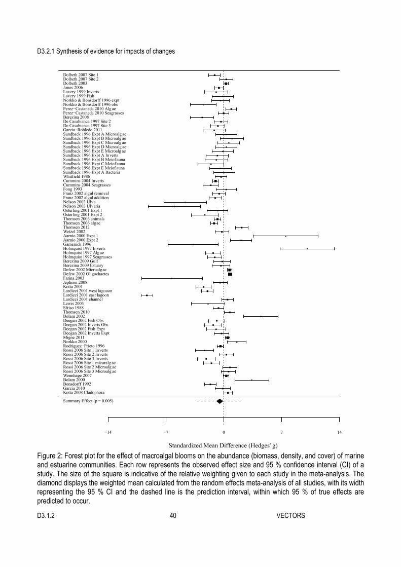
D3.2.1 Synthesis of evidence for impacts of changes  

D3.1.2 40 VECTORS

Figure 2: Forest plot for the effect of macroalgal blooms on the abundance (biomass, density, and cover) of marine and estuarine communities. Each row represents the observed effect size and 95 % confidence interval (CI) of a study. The size of the square is indicative of the relative weighting given to each study in the meta-analysis. The diamond displays the weighted mean calculated from the random effects meta-analysis of all studies, with its width representing the 95 % CI and the dashed line is the prediction interval, within which 95 % of true effects are predicted to occur.

Summary Effect (p = 0.005)

−14 −7 0 7 14

Standardized Mean Difference (Hedges' g)

Kotta 2008 CladophoraGarcia 2010Bonsdorff 1992Bolam 2000Wennhage 2007Rossi 2006 Site 3 Microalg aeRossi 2006 Site 2 Microalg aeRossi 2006 Site 1 micoralg aeRossi 2006 Site 3 InvertsRossi 2006 Site 2 InvertsRossi 2006 Site 1 InvertsRodriguez−Prieto 1996Norkko 2000Migne 2011Deegan 2002 Inverts ExptDeegan 2002 Fish ExptDeegan 2002 Inverts ObsDeegan 2002 Fish ObsBolam 2002Thomsen 2010Sfriso 1988Lewis 2003Lardicci 2001 channelLardicci 2001 east lagoonLardicci 2001 west lagooonKotta 2001Jephson 2008Farina 2003Defew 2002 OligochaetesDefew 2002 MicroalgaeBerezina 2009 EstuaryBerezina 2009 GulfHolmquist 1997 SeagrassesHolmquist 1997 AlgaeHolmquist 1997 InvertsGamenick 1996Aarnio 2000 Expt 2Aarnio 2000 Expt 1Wetzel 2002Thomsen 2012Thomsen 2006 algaeThomsen 2006 animalsOsterling 2001 Expt 2Osterling 2001 Expt 1Nelson 2003 UlvariaNelson 2003 UlvaFranz 2002 algal addition Franz 2002 algal removal Fong 1993Cummins 2004 SeagrassesCummins 2004 InvertsWhitfield 1986Sundback 1996 Expt A BacteriaSundback 1996 Expt E Meiof aunaSundback 1996 Expt C Meiof aunaSundback 1996 Expt B Meiof aunaSundback 1996 Expt A InvertsSundback 1996 Expt E Microalg aeSundback 1996 Expt D Microalg aeSundback 1996 Expt C Microalg aeSundback 1996 Expt B Microalg aeSundback 1996 Expt A Microalg aeGarcia−Robledo 2011De Casabianca 1997 Site 3De Casabianca 1997 Site 2Berezina 2008Perez−Castaneda 2010 SeagrassesPerez−Castaneda 2010 Alg aeNorkko & Bonsdorff 1996 obsNorkko & Bonsdorff 1996 exptLavery 1999 FishLavery 1999 InvertsJones 2006Dolbeth 2003Dolbeth 2007 Site 2Dolbeth 2007 Site 1

D3.2.1 Synthesis of evidence for impacts of changes  

D3.1.2 41 VECTORS

Figure 3: Hedges’ g (± 95 % C.I.) for the effects of macroalgal blooms on community abundance in 13 different marine regions, estimated using a mixed model meta-analysis. The number below each effect size estimate is the number of studies found for that region. The vertical dashed line indicates no effect and the vertical dotted line indicates the mean effect estimated in the overall analysis.

1

16

3

5

1

7

29

6

1

2

2

1

2

Agulhas Current

Baltic Sea

California Current

Gulf of Mexico

Humboldt Current

Mediterranean Sea

NE Atlantic

NE US Continental Shelf

Patagonian Shelf

SE Australian Shelf

SE US Continental Shelf

SW Australian Shelf

West−Central Australian Shelf

−10 −5 0 5Hedges' g

D3.2.1 Synthesis of evidence for impacts of changes  

D3.1.2 42 VECTORS

Figure 4: Hedges’ g (± 95 % C.I.) for the effects of macroalgal blooms on community abundance, summarized according to (A) algal groups, (B) habitats, (C) community types, (D) abundance measures, (E) study types, and (F) study settings. All effects were estimated using a mixed model meta-analysis model. The number below each effect size estimate is the number of studies found for that algal group. The vertical dashed line indicates no effect and the vertical dotted line indicates the mean effect estimated in the overall analysis.

1

4

2

2

3

3

21

38

1

1

CladophoraDigenia

FucusFurcellariaGracilariaLaurencia

MixUlva

UlvariaVaucheria

−10 −5 0 5Hedges' g

A

21

2

2

1

1

22

27

Intertidal sand/mud

Oyster reef

Pelagic

Rocky intertidal

Rocky subtidal

Subtidal sand/mud

Subtidal seagrass bed

−8 −4 0Hedges' g

B

1

4

45

4

16

3

3

Bacteria

Fish

Invertebrates

Macroalgae

Microalgae

Mix

Seagrasses

−2 0 2Hedges' g

C

30

44

2

Biomass

Cover

Density

−3 −2 −1 0 1Hedges' g

D

45

31

Experiment

Observation

−1.0 −0.5 0.0Hedges' g

E

58

18

Field

Lab

−0.8 −0.4 0.0 0.4Hedges' g

F

D3.2.1 Synthesis of evidence for impacts of changes  

D3.1.2 43 VECTORS

Figure 5: Forest plot for the effect of macroalgal blooms on the species richness of marine and estuarine communities. Each row represents the observed effect size and 95 % confidence interval (C.I.) of a study. The size of the square is indicative of the relative weighting given to each study in the meta-analysis. The diamond displays the weighted mean calculated from the random effects meta-analysis of all studies, with its width representing the 95 % CI and the dashed line is the prediction interval, within which 95 % of true effects are predicted to occur.

Summary Effect (p = 0.010)

−20 −10 0 10 20

Standardized Mean Difference (Hedges' g)

Bonsdorff 1992

Bolam 2000

Rossi 2006 Site 3

Rossi 2006 Site 2

Rossi 2006 Site 1

Rodriguez−Prieto 1996

Deegan 2002 Decapods

Deegan 2002 FishBolam 2002

Thomsen 2010

Ouisse 2011

Lewis 2003Lardicci 2001 channel

Lardicci 2001 east lagoon

Lardicci 2001 west lagooon

Farina 2003

Holmquist 1997

Gamenick 1996Wetzel 2002

Thomsen 2012

Thomsen 2006 algae

Thomsen 2006 invertsFranz 2002 algal addition

Franz 2002 algal removal

Cummins 2004Norkko & Bonsdorff 1996 obs

Norkko & Bonsdorff 1996 expt

Lavery 1999 Fish

Lavery 1999 InvertsJones 2006

Dolbeth 2003

Martinetto 2010

Dolbeth 2007 Site 2

Dolbeth 2007 Site 1

D3.2.1 Synthesis of evidence for impacts of changes  

D3.1.2 44 VECTORS

Figure 6: Hedges’ g (± 95 % C.I.) for the effects of macroalgal blooms on species richness, summarized according to (A) algal groups, (B) habitats, (C) community types, (D) abundance measures, (E) study types, and (F) study settings. All effects were estimated using mixed model meta-analysis models. The number below each effect size estimate is the number of studies found for that algal group. The vertical dashed line indicates no effect and the vertical dotted line indicates the mean effect estimated in the overall analysis.

5

1

1

4

12

4

1

1

2

1

2

Baltic SeaGulf of Mexico

Humboldt CurrentMediterranean Sea

NE AtlanticNE US Cont. Shelf

Patagonian ShelfSE Aus. Shelf

SE US Cont. ShelfSW Aus. Shelf

W−Central Aus. Shelf

−10 −5 0 5 10 15Hedges' g

A

3

2

2

1

10

15

1

Cladophora

Fucus

Gracilaria

Laurencia

Mix

Ulva

Vaucheria

−5 0 5 10 15Hedges' g

B

15

2

1

1

9

6

Intertidal sand/mud

Oyster reef

Rocky intertidal

Rocky subtidal

Subtidal sand/mud

Subtidal seagrass bed

−8 −4 0Hedges' g

C

1

2

25

2

4

Birds

Fish

Invertebrates

Macroalgae

Mix

−2 0 2Hedges' g

D

19

15

Experiment

Observation

−1.5 −1.0 −0.5 0.0Hedges' g

E

33

1

Field

Lab

−4 −3 −2 −1 0 1Hedges' g

F

D3.2.1 Synthesis of evidence for impacts of changes  

D3.1.2 45 VECTORS

Figure 7: Forest plot for the effect of macroalgal blooms on the diversity of marine and estuarine communities. Each row represents the observed effect size and 95 % confidence interval (C.I.) of a study. The size of the square is indicative of the relative weighting given to each study in the meta-analysis. The diamond displays the weighted mean calculated from the random effects meta-analysis of all studies, with its width representing the 95 % CI and the dashed line is the prediction interval, within which 95 % of true effects are predicted to occur. .

Summary Effect (p = 0.056)

−15 −10 −5 0 5

Standardized Mean Difference (Hedges' g)

Norkko et al 2000

Lewis 2003

Lardicci 2001 channel

Lardicci 2001 east lagoon

Lardicci 2001 west lagooon

Guo 2011

Gamenick 1996

Wetzel 2002

Thomsen 2012

Norkko & Bonsdorff 1996 obs

Norkko & Bonsdorff 1996 expt

Dolbeth 2003

Martinetto 2010

D3.2.1 Synthesis of evidence for impacts of changes  

D3.1.2 46 VECTORS

Figure 8: Hedges’ g (± 95 % C.I.) for the effects of macroalgal blooms on community diversity, summarized according to (A) marine regions, (B) algal groups, (C) habitats, (D) community types, and (E) study types. All effects were estimated using mixed model meta-analysis models. The number below each effect size estimate is the number of studies found for that algal group. The vertical dashed line indicates no effect and the vertical dotted line indicates the mean effect estimated in the overall analysis.

5

3

2

1

1

1

Baltic Sea

Mediterranean Sea

NE Atlantic

Patagonian Shelf

SW Aus. Shelf

Yellow Sea

−3 0 3 6Hedges' g

A

3

2

1

4

3

Cladophora

Fucus

Gracilaria

Mix

Ulva

−5.0 −2.5 0.0 2.5Hedges' g

B

3

1

8

1

Intertidal sand/mud

Pelagic

Subtidal sand/mud

Subtidal seagrass bed

−4 −2 0 2 4Hedges' g

C

1

11

1

Bacteria

Invertebrates

Mix

−2 0 2 4Hedges' g

D

5

8

Experiment

Observation

−2 −1 0Hedges' g

E

D3.2.1 Synthesis of evidence for impacts of changes  

D3.1.2 47 VECTORS

Figure 9: Forest plot for the effect of macroalgal blooms on the evenness of marine and estuarine communities. Each row represents the observed effect size and 95 % confidence interval (C.I.) of a study. The size of the square is indicative of the relative weighting given to each study in the meta-analysis. The diamond displays the weighted mean calculated from the random effects meta-analysis of all studies, with its width representing the 95 % CI and the dashed line is the prediction interval, within which 95 % of true effects are predicted to occur.

Summary Effect (p = 0.884)

−90 −65 −40 −15 10

Standardized Mean Difference (Hedges' g)

Norkko et al 2000

Lewis 2003

Gamenick 1996

Wetzel 2002

Thomsen 2012

Norkko & Bonsdorff 1996 obs

Norkko & Bonsdorff 1996 expt

D3.2.1 Synthesis of evidence for impacts of changes  

D3.1.2 48 VECTORS

Figure 10: Hedges’ g (± 95 % C.I.) for the effects of macroalgal blooms on community evenness, summarized according to (A) marine regions, (B) algal groups, (C) habitats, and (D) study types. All effects were estimated using a mixed model meta-analysis model. The number below each effect size estimate is the number of studies found for that algal group. The vertical dashed line indicates no effect and the vertical dotted line indicates the mean effect estimated in the overall analysis.

5

1

1

Baltic Sea

NE Atlantic

SW Aus. Shelf

−4 −2 0 2 4Hedges' g

A

2

1

3

1

Fucus

Gracilaria

Mix

Ulva

−5.0 −2.5 0.0 2.5 5.0Hedges' g

B

1

5

1

Intertidal sand/mud

Subtidal sand/mud

Subtidal seagrass bed

−4 −2 0 2 4Hedges' g

C

5

2

Experiment

Observation

−2 −1 0 1 2Hedges' g

D

D3.2.1 Synthesis of evidence for impacts of changes  

D3.1.2 49 VECTORS

Figure 11: Forest plot for the effect of macroalgal blooms on the gross primary productivity of marine and estuarine communities. Each row represents the observed effect size and 95 % confidence interval (C.I.) of a study. The size of the square is indicative of the relative weighting given to each study in the meta-analysis. The diamond displays the weighted mean calculated from the random effects meta-analysis of all studies, with its width representing the 95 % CI and the dashed line is the prediction interval, within which 95 % of true effects are predicted to occur.

Mean Effect (p < 0.001)

−7 −3.5 0 3.5 7

Standardized Mean Difference (Hedges' g)

Migne 2011

Corzo 2009

Cacabelos 2012

Hubas 2006

Dalsgaard 2003 Ulbjerg

Dalsgaard 2003 Virksund

D3.2.1 Synthesis of evidence for impacts of changes  

D3.1.2 50 VECTORS

Figure 12: Hedges’ g (± 95 % C.I.) for the effects of macroalgal blooms on gross primary productivity, summarized according to (A) algal groups, (B) habitats, (C) study types, and (D) study settings. All effects were estimated using a mixed model meta-analysis model. The number below each effect size estimate is the number of studies found for that algal group. The vertical dashed line indicates no effect and the vertical dotted line indicates the mean effect estimated in the overall analysis.

1

1

4

Gracilaria

Mix

Ulva

−3 0 3 6Hedges' g

A

3

1

2

Intertidal sand/mud

Intertidal seagrass beds

Subtidal sand/mud

−2.5 0.0 2.5 5.0Hedges' g

B

1

5

Experiment

Observational

−2.5 0.0 2.5Hedges' g

C

3

3

Field

Lab

0 1 2 3 4 5Hedges' g

D

D3.2.1 Synthesis of evidence for impacts of changes  

D3.1.2 51 VECTORS

Figure 13: Forest plot for the effect of macroalgal blooms on the net primary productivity of marine and estuarine communities. Each row represents the observed effect size and 95 % confidence interval (C.I.) of a study. Studies including macroalgal productivity in their estimates are represented by closed squares and studies that excluded macroalgal productivity are represented by open squares. The size of the square is indicative of the relative weighting given to each study in the meta-analysis. The diamond displays the weighted mean calculated from the random effects meta-analysis of all studies, with its width representing the 95 % CI and the dashed line is the prediction interval, within which 95 % of true effects are predicted to occur.

Summary Effect (p = 0.7608)

−10 −5 0 5 10

Standardized Mean Difference (Hedges' g)

Corzo 2009

Cacabelos 2012

Engelsen 2008

Sundback 1996 Expt D

Qu 2003

Garcia−Robledo 2011

Dalsgaard 2003 Ulbjerg

Dalsgaard 2003 Virksund

D3.2.1 Synthesis of evidence for impacts of changes  

D3.1.2 52 VECTORS

Figure 14: Hedges’ g (± 95 % C.I.) for the effects of macroalgal blooms on net primary productivity, summarized according to (A) region, (B) algal groups, (C) habitats, (D) measurement methods (methods that include or exclude the productivity of the bloom algae), (E) study types, and (F) study settings. All effects were estimated using a mixed model meta-analysis model. The number below each effect size estimate is the number of studies found for that algal group. The vertical dashed line indicates no effect and the vertical dotted line indicates the mean effect estimated in the overall analysis.

1

1

6

Baltic Sea

E−Central Aus. Shelf

NE Atlantic

−5 0 5 10Hedges' g

A

1

1

1

5

Chaetomorpha

Gracilaria

Mix

Ulva

−5 0 5 10Hedges' g

B

2

1

3

2

Intertidal sand/mud

Intertidal seagrass beds

Subtidal sand/mud

Subtidal seagrass bed

−8 −4 0 4Hedges' g

C

5

3Excluding macroalgae

Including macroalgae

−6 −4 −2 0 2 4Hedges' g

D

4

4

Experiment

Observational

−5.0 −2.5 0.0 2.5 5.0Hedges' g

E

1

7

Field

Lab

−10 −5 0Hedges' g

F

D3.2.1 Synthesis of evidence for impacts of changes  

D3.1.2 53 VECTORS

Figure 15: Forest plot for the effect of macroalgal blooms on the respiration of marine and estuarine communities. Each row represents the observed effect size and 95 % confidence interval (C.I.) of a study. Studies including macroalgal respiration in their estimates are represented by closed squares and studies that excluded macroalgal respiration are represented by open squares. The size of the square is indicative of the relative weighting given to each study in the meta-analysis. The diamond displays the weighted mean calculated from the random effects meta-analysis of all studies, with its width representing the 95 % CI and the dashed line is the prediction interval, within which 95 % of true effects are predicted to occur.

Mean Effect (p = 0.1473)

−3 0 3 6 9

Standardized Mean Difference (Hedges' g)

Migne 2011

Corzo 2009

Cacabelos 2012

Hubas 2006

Qu 2003

Garcia−Robledo 2011

Auffrey 2004

Dalsgaard 2003 Ulbjerg

Dalsgaard 2003 Virksund

D3.2.1 Synthesis of evidence for impacts of changes  

D3.1.2 54 VECTORS

Figure 16: Hedges’ g (± 95 % C.I.) for the effects of macroalgal blooms on community respiration, summarized according to (A) region, (B) algal groups, (C) habitats, (D) measurement methods (methods that include or exclude the respiration of the bloom algae) / study type and (E) study settings. Measurement methods and study type were completely confounded and are presented together. The number below each effect size estimate is the number of studies found for that algal group. The vertical dashed line indicates no effect and the vertical dotted line indicates the mean effect estimated in the overall analysis. Note that the analyses for measurement methods and study type are completely confounded.

1

7

1

E−Central Aus. Self

NE Atlantic

Scotian Shelf

−2.5 0.0 2.5 5.0Hedges' g

A

1

1

2

5

Chaetomorpha

Gracilaria

Mix

Ulva

−2.5 0.0 2.5 5.0Hedges' g

B

5

1

2

1

Intertidal sand/mud

Intertidal seagrass beds

Subtidal sand/mud

Subtidal seagrass bed

−2.5 0.0 2.5 5.0Hedges' g

C

7

2Excluding macroalgae/

Experimental

Including macroalgae/ Observational

−2 0 2Hedges' g

D

4

5

Field

Lab

−1 0 1 2 3Hedges' g

E

D3.2.1 Synthesis of evidence for impacts of changes  

D3.1.2 55 VECTORS

Figure 17: Funnel plots for the overall meta-analyses for the effects of macroalgal blooms on (A) community abundance, (B) species richness, (C) diversity (Shannon index), (D) evenness (Pielou’s index), (E) gross primary productivity, (F) net primary productivity, (G) respiration, and (H) net primary productivity, adjusted for the effect of measurement methods. Each point represents the values of a single study. The vertical line is located at the value of the summary effect for the overall analyses (plots A-G) or at zero for the subgroup analysis (H). The white area bordered by the dashed lines is the pseudo-confidence region within which 95 % of studies are expected to fall in the absence of among study heterogeneity and publication bias. The x-axis is Hedges’ g for all plots, except for plot H, which uses the residual value for each study. Rank correlation tests indicated that none of the funnel plots were asymmetrical (p > 0.129).

2.0

1.5

1.0

0.5

0.0

−10.0 −5.0 0.0 5.0 10.0

A

2.4

1.8

1.2

0.6

0.0

−15.0 −10.0 −5.0 0.0 5.0 10.0

B

3.0

2.2

1.5

0.7

0.0

−5.0 0.0 5.0

C

Sta

ndar

d E

rror

17.4

8.7

4.3

0.0

−40.0 −20.0 0.0 20.0 40.0

D

1.0

0.7

0.5

0.2

0.0

1.0 2.0 3.0 4.0 5.0

E

1.7

1.3

0.9

0.4

0.0

−6.0 −4.0 −2.0 0.0 2.0 4.0

F

1.0

0.7

0.5

0.2

0.0

−2.0 0.0 2.0 4.0 6.0

G

Hedges' g or Residual Value

1.7

1.3

0.9

0.4

0.0

−4.0 −2.0 0.0 2.0 4.0

H

D3.2.1 Synthesis of evidence for impacts of changes  

D3.1.2 56 VECTORS

Annex A: Search terms used to find relevant studies We searched for relevant studies in Web of Science and Scopus online databases using two complex sets search terms. To identity studies involving macroalgal blooms we used: (((Enteromorpha OR Ulva OR ulvoid OR Ulvaria OR Gracilaria OR "Pilayella littoralis" OR Cladophora OR Chaetomorpha OR Pylaiella OR Ectocarpus OR Lobophora OR wrack ) AND (bloom* OR outbreak OR proliferation OR overabundance )) OR "green tide" OR "macroalgal bloom*" OR "seaweed bloom* " OR "macroalgal accumulation*" OR "accumulation* of macroalga*" OR "alga* mat" OR "alga* mats" OR "macroalgal mat*" OR "accumulation* of algae" OR "drifting alga*" OR "drifting macroalg*" OR "nuisance macroalga*" OR "ephemeral alga*" OR "opportunistic alga*" OR (("Alga* bloom*" OR "alga* outbreak*" OR "Nuisance alga*" ) AND (wrack OR seaweed OR macroalga* OR Enteromorpha OR Ulva OR Ulvaria OR Gracilaria OR Pilayella OR Cladophora OR Chaetomorpha OR Pylaiella OR Ectocarpus OR Lobophora ))) This set was combined with a second set intended to identify studies that examined the effects of macroalgal blooms on ecosystem structure and functioning: ((hysteresis OR "tipping point" OR "alternat* state" OR "alternat* stable state" OR "phase shift" OR "regime shift" OR "species richness" OR diversity OR "community structure" OR evenness OR "Shannon-Weaver" OR "Shannon-Weiner" OR "Shannon index" OR "Simpson Index" OR "abundance biomass curve*" OR "species abundance distribution*") OR ("Energy flow*" OR "Energy flux*" OR "Flow* of energy"OR "Flux* of energy" OR biogeochemical OR "Nutrient cycl*" OR "cycling of nutrient*" OR "Nutrient dynamics" OR "nutrient flux*" OR "Nutrient flow*" OR "Flow* of nutrient*" OR "Flux* of nutrient*" OR "cycling of carbon" OR "carbon cycl*" OR "carbon stor*" OR "carbon flow*" OR "carbon flux*" OR "flow* of carbon" OR "flux* of carbon" OR "cycling of sul*ur" OR "Sul*ur cycl*" OR "Flow* of sul*ur" OR "flux* of sul*ur" OR "sul*ur flux*" OR "sul*ur flow*" OR "Hydrogen sul*ide" OR "cycling of nitrogen" OR "nitrogen cycl*" OR "Flow* of nitrogen" OR "flux* of nitrogen" OR "nitrogen flux*" OR "nitrogen flow*" OR denitrification OR "cycling of phosphorus" OR " phosphorus cycl*" OR "Flow* of phosphorus" OR "flux* of phosphorus" OR "phosphorus flux*" OR "phosphorus flow*" OR "cycling of oxygen" OR " oxygen cycl*" OR "Flow* of oxygen" OR "flux* of oxygen" OR "oxygen flux*" OR "oxygen flow*" OR anoxi* OR hypoxi* OR bioturbation OR grazing OR foraging OR herbivory OR predation) OR ("primary product*" OR "secondary product*" OR "carbon fixation" OR "community respiration" OR "ecosystem respiration" OR "community metabolism" OR "ecosystem metabolism" OR "abundance of benthic" OR "productivity of benthic" OR "benthic biomass" OR "biomass of benthic" OR "benthic metabolism" OR "benthic respiration" OR ((abundance* OR biomass* OR productivity OR mortalit* OR survival OR growth OR cover OR densit*) AND (fauna* OR animal OR infauna* OR epifauna* OR fish OR macroinvertebrate OR invertebrate OR macrofauna* OR mesofauna* OR meiofauna* OR epibenthic OR seagrass OR eelgrass OR Cymodocea OR Zostera OR Posidonia OR seaweed OR macroalgal OR macroalgae OR fish* OR bird* OR seabird OR shorebird))))

D3.2.1 Synthesis of evidence for impacts of changes  

D3.1.2 57 VECTORS

Annex B: Papers included in the meta-analysis. AARNIO, K. & MATTILA, J. 2000. Predation by juvenile Platichthys flesus (L.) on shelled prey species in a bare sand and a drift algae habitat. Hydrobiologia, 440, 347-355. AUFFREY, L. M., ROBINSON, S. M. C. & BARBEAU, M. A. 2004. Effect of green macroalgal mats on burial depth of soft-shelled clams Mya arenaria. Marine Ecology Progress Series, 278, 193-203. BEREZINA, N. A. & GOLUBKOV, S. M. Responses of coastal zoobenthos to stress induced by drifting algae in the Neva estuary. US/EU-Baltic International Symposium: Ocean Observations, Ecosystem-Based Management and Forecasting - Provisional Symposium Proceedings, BALTIC, 2008. BEREZINA, N. A., GOLUBKOV, S. M. & GUBELIT, Y. I. 2009. Structure of littoral zoocenoses in the macroalgae zones of the Neva River Estuary. Inland Water Biology, 2, 340-347. BOLAM, S. G. & FERNANDES, T. F. 2002. The effects of macroalgal cover on the spatial distribution of macrobenthic invertebrates: the effect of macroalgal morphology. Hydrobiologia, 475, 437-448. BOLAM, S. G., FERNANDES, T. F., READ, P. & RAFFAELLI, D. 2000. Effects of macroalgal mats on intertidal sandflats: an experimental study. Journal of Experimental Marine Biology and Ecology, 249, 123-137. BONSDORFF, E. 1992. Drifting algae and zoobenthos - effects on settling and community structure. Netherlands Journal of Sea Research, 30, 57-62. CACABELOS, E., ENGELEN, A. H., MEJIA, A. & ARENAS, F. 2012. Comparison of the assemblage functioning of estuary systems dominated by the seagrass Nanozostera noltii versus the invasive drift seaweed Gracilaria vermiculophylla. Journal of Sea Research, 72, 99-105. CORZO, A., VAN BERGEIJK, S. A. & GARCIA-ROBLEDO, E. 2009. Effects of green macroalgal blooms on intertidal sediments: net metabolism and carbon and nitrogen contents. Marine Ecology Progress Series, 380, 81-93. CUMMINS, S. P., ROBERTS, D. E. & ZIMMERMAN, K. D. 2004. Effects of the green macroalga Enteromorpha intestinalis on macrobenthic and seagrass assemblages in a shallow coastal estuary. Marine Ecology Progress Series, 266, 77-87. DALSGAARD, T. 2003. Benthic primary production and nutrient cycling in sediments with benthic microalgae and transient accumulation of macroalgae. Limnology and Oceanography, 48, 2138-2150. DE CASABIANCA, M. L., LAUGIER, T. & MARINHO-SORIANO, E. 1997. Seasonal changes of nutrients in water and sediment in a Mediterranean lagoon with shellfish farming activity (Thau Lagoon, France). Ices Journal of Marine Science, 54, 905-916. DEEGAN, L. A., WRIGHT, A., AYVAZIAN, S. G., FINN, J. T., GOLDEN, H., MERSON, R. R. & HARRISON, J. 2002. Nitrogen loading alters seagrass ecosystem structure and support of higher trophic levels. Aquatic Conservation-Marine and Freshwater Ecosystems, 12, 193-212. DEFEW, E. C., TOLHURST, T. J. & PATERSON, D. M. 2002. Site-specific features influence sediment stability of

D3.2.1 Synthesis of evidence for impacts of changes  

D3.1.2 58 VECTORS

intertidal flats. Hydrology and Earth System Sciences, 6, 971-981. DOLBETH, M., CARDOSO, P. G., FERREIRA, S. M., VERDELHOS, T., RAFFAELLI, D. & PARDAL, M. A. 2007. Anthropogenic and natural disturbance effects on a macrobenthic estuarine community over a 10-year period. Marine Pollution Bulletin, 54, 576-585. DOLBETH, M., PARDAL, M. A., LILLEBO, A. I., AZEITEIRO, U. & MARQUES, J. C. 2003. Short- and long-term effects of eutrophication on the secondary production of an intertidal macrobenthic community. Marine Biology, 143, 1229-1238. ENGELSEN, A. & PIHL, L. 2008. Grazing effects by Nereis diversicolor on development and growth of green algal mats. Journal of Sea Research, 59, 228-236. FARINA, J. M., CASTILLA, J. C. & OJEDA, F. P. 2003. The "idiosyncratic" effect of a "sentinel" species on contaminated rocky intertidal communities. Ecological Applications, 13, 1533-1552. FONG, P., DONOHOE, R. M. & ZEDLER, J. B. 1993. Competition with macroalgae and benthic cyanobacterial mats limits phytoplankton abundance in experimental microcosms. Marine Ecology Progress Series, 100, 97-102. FRANZ, D. R. & FRIEDMAN, I. 2002. Effects of a macroalgal mat (Ulva lactuca) on estuarine sand flat copepods: an experimental study. Journal of Experimental Marine Biology and Ecology, 271, 209-226. GAMENICK, I., JAHN, A., VOPEL, K. & GIERE, O. 1996. Hypoxia and sulphide as structuring factors in a macrozoobenthic community on the Baltic Sea shore: colonisation studies and tolerance experiments. Marine Ecology Progress Series, 144, 73-85. GARCIA, G. O., ISACCH, J. P., LAICH, A. G., ALBANO, M., FAVERO, M., CARDONI, D. A., LUPPI, T. & IRIBARNE, O. 2010. Foraging behaviour and diet of American Oystercatchers in a Patagonian intertidal area affected by nutrient loading. Emu, 110, 146-154. GARCÍA-ROBLEDO, E. & CORZO, A. 2011. Effects of macroalgal blooms on carbon and nitrogen biogeochemical cycling in photoautotrophic sediments: An experimental mesocosm. Marine Pollution Bulletin, 62, 1550-1556. GUO, C., LI, F. C., JIANG, P., LIU, Z. P. & QIN, S. 2011. Bacterial diversity in surface water of the Yellow Sea during and after a green alga tide in 2008. Chinese Journal of Oceanology and Limnology, 29, 1147-1154. HOLMQUIST, J. G. 1997. Disturbance and gap formation in a marine benthic mosaic: influence of shifting macroalgal patches on seagrass structure and mobile invertebrates. Marine Ecology Progress Series, 158, 121-130. HUBAS, C. & DAVOULT, D. 2006. Does seasonal proliferation of Enteromorpha sp. affect the annual benthic metabolism of a small macrotidal estuary? (Roscoff Aber Bay, France). Estuarine Coastal and Shelf Science, 70, 287-296. JEPHSON, T., NYSTROM, P., MOKSNES, P. O. & BADEN, S. P. 2008. Trophic interactions in Zostera marina beds along the Swedish coast. Marine Ecology Progress Series, 369, 63-76. JONES, M. & PINN, E. 2006. The impact of a macroalgal mat on benthic biodiversity in Poole Harbour. Marine

D3.2.1 Synthesis of evidence for impacts of changes  

D3.1.2 59 VECTORS

Pollution Bulletin, 53, 63-71. KOTTA, J. & ORAV, H. 2001. Role of benthic macroalgae in regulating macrozoobenthic assemblages in the Vainameri (north-eastern Baltic Sea). Annales Zoologici Fennici, 38, 163-171. KOTTA, J., PAALME, T., PUSS, T., HERKUL, K. & KOTTA, I. 2008. Contribution of scale-dependent environmental variability on the biomass patterns of drift algae and associated invertebrates in the Gulf of Riga, northern Baltic Sea. Journal of Marine Systems, 74, S116-S123. LARDICCI, C., COMO, S., CORTI, S. & ROSSI, F. 2001. Recovery of the macrozoobenthic community after severe dystrophic crises in a Mediterranean coastal lagoon (Orbetello, Italy). Marine Pollution Bulletin, 42, 202-214. LAVERY, P., BOOTLE, S. & VANDERKLIFT, M. 1999. Ecological effects of macroalgal harvesting on beaches in the Peel-Harvey estuary, Western Australia. Estuarine Coastal and Shelf Science, 49, 295-309. LEWIS, L. J., DAVENPORT, J. & KELLY, T. C. 2003. Responses of benthic invertebrates and their avian predators to the experimental removal of macroalgal mats. Journal of the Marine Biological Association of the United Kingdom, 83, 31-36. MARTINETTO, P., DALEO, P., ESCAPA, M., ALBERTI, J., ISACCH, J. P., FANJUL, E., BOTTO, F., PIRIZ, M. L., PONCE, G., CASAS, G. & IRIBARNE, O. 2010. High abundance and diversity of consumers associated with eutrophic areas in a semi-desert macrotidal coastal ecosystem in Patagonia, Argentina. Estuarine Coastal and Shelf Science, 88, 357-364. MIGNE, A., OUISSE, V., HUBAS, C. & DAVOULT, D. 2011. Freshwater seepages and ephemeral macroalgae proliferation in an intertidal bay: II. Effect on benthic biomass and metabolism. Estuarine Coastal and Shelf Science, 92, 161-168. NELSON, T. A., LEE, D. J. & SMITH, B. C. 2003. Are "green tides" harmful algal blooms? Toxic properties of water-soluble extracts from two bloom-forming macroalgae, Ulva fenestrata and Ulvaria obscura (Ulvophyceae). Journal of Phycology, 39, 874-879. NORKKO, A. & BONSDORFF, E. 1996. Rapid zoobenthic community responses to accumulations of drifting algae. Marine Ecology Progress Series, 131, 143-157. NORKKO, J., BONSDORFF, E. & NORKKO, A. 2000. Drifting algal mats as an alternative habitat for benthic invertebrates: Species specific responses to a transient resource. Journal of Experimental Marine Biology and Ecology, 248, 79-104. ÖSTERLING, M. & PIHL, L. 2001. Effects of filamentous green algal mats on benthic macrofaunal functional feeding groups. Journal of Experimental Marine Biology and Ecology, 263, 159-183. OUISSE, V., RIERA, P., MIGNE, A., LEROUX, C. & DAVOULT, D. 2011. Freshwater seepages and ephemeral macroalgae proliferation in an intertidal bay: I Effect on benthic community structure and food web. Estuarine Coastal and Shelf Science, 91, 272-281. PEREZ-CASTANEDA, R., BLANCO-MARTINEZ, Z., SANCHEZ-MARTINEZ, J. G., RABAGO-CASTRO, J. L.,

D3.2.1 Synthesis of evidence for impacts of changes  

D3.1.2 60 VECTORS

AGUIRRE-GUZMAN, G. & VAZQUEZ-SAUCEDA, M. D. 2010. Distribution of Farfantepenaeus aztecus and F. duorarum on submerged aquatic vegetation habitats along a subtropical coastal lagoon (Laguna Madre, Mexico). Journal of the Marine Biological Association of the United Kingdom, 90, 445-452. QU, W. C., MORRISON, R. J. & WEST, R. J. 2003. Inorganic nutrient and oxygen fluxes across the sediment-water interface in the inshore macrophyte areas of a shallow estuary (Lake Illawarra, Australia). Hydrobiologia, 492, 119-127. ROSSI, F. 2006. Small-scale burial of macroalgal detritus in marine sediments: Effects of Ulva spp. on the spatial distribution of macrofauna assemblages. Journal of Experimental Marine Biology and Ecology, 332, 84-95. SFRISO, A., PAVONI, B., MARCOMINI, A. & ORIO, A. A. 1988. Annual variations of nutrients in the Lagoon of Venice. Marine Pollution Bulletin, 19, 54-60. SUNDBACK, K., CARLSON, L., NILSSON, C., JONSSON, B., WULFF, A. & ODMARK, S. 1996. Response of benthic microbial mats to drifting green algal mats. Aquatic Microbial Ecology, 10, 195-208. THOMSEN, M. S. 2010. Experimental evidence for positive effects of invasive seaweed on native invertebrates via habitat-formation in a seagrass bed. Aquatic Invasions, 5, 341-346. THOMSEN, M. S., DE BETTIGNIES, T., WERNBERG, T., HOLMER, M. & DEBEUF, B. 2012. Harmful algae are not harmful to everyone. Harmful Algae, 16, 74-80. THOMSEN, M. S. & MCGLATHERY, K. 2006. Effects of accumulations of sediments and drift algae on recruitment of sessile organisms associated with oyster reefs. Journal of Experimental Marine Biology and Ecology, 328, 22-34. WENNHAGE, H. & PIHL, L. 2007. From flatfish to sticklebacks: assemblage structure of epibenthic fauna in relation to macroalgal blooms. Marine Ecology Progress Series, 335, 187-198. WETZEL, M. A., WEBER, A. & GIERE, O. 2002. Re-colonization of anoxic/sulfidic sediments by marine nematodes after experimental removal of macroalgal cover. Marine Biology, 141, 679-689. WHITFIELD, A. K. 1986. Fish community structure response to major habitat changes within the littoral zone of an estuarine coastal lake. Environmental Biology of Fishes, 17, 41-51.

D3.2.1 Synthesis of evidence for impacts of changes  

D3.1.2 61 VECTORS

Annex C: List of references that could not be accessed at full text. This list includes papers that could not accessed, conference abstracts, and publications in languages other than English. MELTON, M. & NELSON, T. A. 2011. STABLE ISOTOPE ANALYSIS AND UNDERWATER VIDEO SHOW IMPORTANCE OF HIGHLY LOCALIZED FACTORS IN CONTRIBUTING TO EXCESSIVE GROWTH OF HARMFUL MACROALGAL BLOOMS. Journal of Phycology, 47, S84-S84. Reason: Conference Abstract NEWTON, C. & THORNBER, C. 2011. ABUNDANCE AND DISTRIBUTION SURVEYS OF MACROALGAL BLOOMS IN NEW ENGLAND SALT MARSHES. Journal of Phycology, 47, 35-36. Reason: Conference Abstract NORTH, W. J., STEPHENS, G. C. & NORTH, B. B. 1972. Marine algae and their relation to pollution problems. MARINE POLLUTION AND SEA LIFE, 330-340. Reason: Could not access PINN, E. & JONES, M. 2005. 20. Macroalgal mat development and associated changes in infaunal biodiversity. Proceedings in Marine Science. Reason: Could not access RIISGARD, H. U., CHRISTENSEN, P. B., OLESEN, N. J., PETERSEN, J. K., MOLLER, M. M. & ANDERSEN, P. 1995. BIOLOGICAL STRUCTURE IN A SHALLOW COVE (KERTINGE-NOR, DENMARK) - CONTROL BY BENTHIC NUTRIENT FLUXES AND SUSPENSION-FEEDING ASCIDIANS AND JELLYFISH. Ophelia, 41, 329-344. Reason: Could not access SALOVIUS, S. & KRAUFVELIN, P. 2004. The filamentous green alga Cladophora glolmerata as a habitat for littoral macro-fauna in the northern Baltic Sea. Ophelia, 58, 65-78. Reason: Could not access WU, X. Q., XU, K. D., YU, Z. S., YU, T. T., MENG, Z. C., DAI, R. H. & LEI, Y. L. 2010. Standing crop and spatial distribution of meiofauna in yellow sea at late stage of enteromorpha prolifera bloom in 2008. Chinese Journal of Applied Ecology, 21, 2140-2147. Reason: Chinese Text

D3.2.1 Synthesis of evidence for impacts of changes  

D3.1.2 62 VECTORS

Appendix 2: What are the effects of non-indigenous seaweeds on native benthic assemblages? Variability between trophic levels and influence of background

environmental and biological conditions Fabio Bulleri 1*, Lisandro Benedetti-Cecchi 2, Eva Chatzinikolaou 3, Tasman Crowe 4, Jonne Kotta 5, Devin

Lyons 6, Rebecca Mant 7, Gil Rilov 8, Luca Rindi9, Elena Maggi 10

1 University of Pisa, *fabio.bulleri@unipi.it 2 University of Pisa, lisandro.benedetti.cecchi@unipi.it 3 Hellenic Centre for Marine Research, evachatz@hcmr.gr 4 University College Dublin, tasman.crowe@ucd.ie 5 Estonian Marine Institute, jonne.kotta@sea.ee 6 University College Dublin, devin.lyons@ucd.ie 7 Bangor University, Rebecca.Mant@unep-wcmc.org 8 Israel Oceanographic and Limnological Research, rilovg@ocean.org.il 9 University of Pisa, lrindi@biologia.unipi.it 10 University of Pisa, emaggi@biologia.unipi.it Abstract Background. In the marine environment, the introduction and spread of non-indigenous benthic macroalgae may cause major alterations to native assemblages and biodiversity. We compared the impacts of exotic seaweeds on native consumers (across trophic levels) to those observed on native primary producers (same trophic level). In addition, we assessed variations in the effects of non-indigenous seaweeds on native benthic ecosystems according to the degree of existing human impact (i.e. along a gradient from urban/industrial areas to extra-urban areas to pristine areas). Methods. We searched for both experimental and observational studies on the effects of exotic seaweeds on native assemblages. We summarized effects of exotic seaweeds by calculating standardized mean differences between invaded and non-invaded means (Hedges’ g*), which were used to perform meta-analytical comparisons of interest. Results. Literature search resulted in the extraction of data from both experimental and observational studies (for a total of 122 papers) investigating the effects of 11 different non-indigenous seaweeds on single species or communities. Most of the studies were performed in the European Seas (the Western Mediterranean hosted the largest number of studies), Australia and Atlantic North America. No data were available from Africa or Asia. The effects of non-indigenous seaweeds on native primary producer communities and species were generally negative and greater than those that emerged at higher trophic levels. The analysis of all data indicated that seaweeds caused a significant decrease in the abundance, biomass, diversity and evenness of primary producer communities, likely reflecting the negative effects on the abundance, biomass, growth and survival of singular species. Differently, seaweeds had significant negative effects on consumers only on community biomass and on survival of singular species. This resulted in a significant difference in the effect of exotic seaweeds between primary producers and consumers for abundance and diversity of communities. Of the species investigated, Caulerpa racemosa seemed to be the one able to generate the most remarkable, negative changes on the primary producer communities it invades, which were significantly different from those on consumers for abundance and

D3.2.1 Synthesis of evidence for impacts of changes  

D3.1.2 63 VECTORS

diversity. Results suggested considerable variation in the effects of non-indigenous seaweeds among habitats, but negative effects were particularly severe in the Western Mediterranean. The effects of non-indigenous seaweeds on most of the response variables examined did not vary among areas characterized by a different degree of human impact. However, the effects on the abundance of consumer species changed from clearly negative when in relatively pristine areas to neutral or slightly positive in areas heavily impacted by human activities. A similar trend emerged for community diversity. Discussion. Our results suggest that ecosystems invaded by non-indigenous seaweeds are characterized by lower abundance, diversity, evenness and biomass of primary producers, and that these effects only partially scaled up to higher trophic levels. A negative impact on native primary producers may result in the lessening of important ecosystems services, such as nutrient cycling, carbon storage, mitigation of coastal erosion through the dampening of wave action, reduced amenity and recreational value of coastal areas. In addition, effects on some response variables showed a tendency to be more severe in relatively pristine environments, with possible impingements to the effectiveness of conservation strategies (i.e. Marine Protected Areas) that are generally implemented in areas little exposed to human impacts. Background Biological invasions are an important component of global change, posing major threats to marine biodiversity [1]. The introduction of non-indigenous species can alter the structure and functioning of natural ecosystems, with potential repercussions for their ability to provide goods and services to humans [2,3]. Thus, assessing the impacts of non-indigenous species on native assemblages is among the top priorities for ecologists. In the marine environment, the spread of non-indigenous benthic macroalgae can lead to a complete domination of substrata, strongly affecting native assemblages and biodiversity. The impacts of non-indigenous seaweeds on native macroalgal assemblages have been thoroughly reviewed [4,5]. In contrast, little effort has been put into synthesizing our current knowledge on the effects of exotic seaweeds across trophic levels and, in particular, to compare the effects on primary producers with those on consumers. This is at odds with mounting evidence indicating that exotic seaweeds can be consumed by guilds of native herbivores, which can, in some cases, suffer physiological damage from the ingestion of these novel sources of [6-8]. For instance, in the Mediterranean Sea, the red pigment caulerpin, the most abundant secondary metabolite of the green exotic macroalga, Caulerpa racemosa, enters food chains and accumulates in fish tissues [8]. Under these circumstances, evaluating the magnitude of the impacts of non-indigenous macroalgae at upper trophic levels (i.e. consumers) and how they relate to impacts at the same trophic level (i.e. on native macroalgal assemblages) is of paramount importance for the management of invasions. Addressing bottom-up effects associated with invasions of primary producers will also help to refine current invasion theories that envision the success of invasive species in the introduced range as a result of the loss of consumers or parasites (e.g. enemy-release hypothesis [9]).

In addition, we can predict that the effects of non-indigenous seaweeds on native assemblages will vary according to background physical and biological conditions. Biological and physical attributes of recipient ecosystems (e.g. richness, relative abundance and evenness of species, availability of resources, regime of disturbance) are known to play a key role in determining the susceptibility to invasion of natural communities [10-13]. The same factors may also play a role in determining the severity of the impacts of invaders. In fact, we could predict that species surviving or thriving in heavily degraded habitats are not limited by competition, but rather controlled by unfavorable environmental conditions [14]. Thus, these species are likely to be weakly affected by the presence of

D3.2.1 Synthesis of evidence for impacts of changes  

D3.1.2 64 VECTORS

novel species. In contrast, in well preserved, species-rich environments, competition is thought to be stronger, so that resource uptake by exotic seaweeds could generate strong negative effects on resident species.

Objective of the review

The objective of the review was to fill these two major gaps in our understanding of the impacts of biological invasions, taking advantage of the availability of a large body of empirical studies that have been carried out in marine environments. We looked at the impacts of non-indigenous seaweeds (species that have established outside their native range via human activities) on native assemblages, in order to answer the following primary questions:

a) How does the impact of exotic seaweeds on native consumers (across trophic levels) compare in magnitude and extent to that observed on native primary producers (same trophic level)?

b) Do the effects of exotic seaweeds on native benthic ecosystems vary according to the degree of existing human impact (i.e. along a gradient from urban/industrial areas to extra-urban areas to pristine areas)?

Methods We carried out a systematic review, following our peer-reviewed protocol, currently available in a separate publication [15]. A concise description of our methods, including modifications made to the protocol during the review process, is provided below. Study Inclusion Criteria For the first question (a), we focused on native primary producer and consumer assemblages, populations and individuals (Table 1). For the second question (b), we extended our focus to include the entire benthic assemblage, including benthic macroalgae, invertebrates and fish (Table 2). The geographic scope of this review was global. A modification to the protocol was applied, as we neither did look (as reported in the secondary questions in the protocol) at the influence of latitude, nor of seaweed abundance, on the effects investigated through primary questions a and b. However, comparisons of the effects of exotic seaweeds between primary producers and consumers were also run separately for individual European regional seas, a task not included in the protocol. The need to include a gradient in the degree of human impacts prevented such a European level focus for the second primary question as there were insufficient data. We were interested in response variables describing the structure of assemblages, the characteristics of populations and individuals and the functioning of assemblages (Table 1 and 2). The methodology and the definitions presented in Tables 1 and 2 are described in detail in Bulleri et al. [15], which is available at www.environmentalevidencejournal.org/content/1/1/8. Search Strategy We searched ‘ISI Web of Science’ database for relevant literature and data. ‘JSTOR’ database was not used, due to the need to maximize limited resources. Although ‘JSTOR’ includes contents published earlier than those included in ‘ISI Web of Science’ (which start from 1970), it is worth noting that the first publications about ecological effects of invasive seaweeds date back to the early 1980s [16]. The search was conducted in June 2012.

D3.2.1 Synthesis of evidence for impacts of changes  

D3.1.2 65 VECTORS

Search strings comprised the terms reported in Table 3. The individual terms or phrases listed within each column were combined by ‘OR’ within each category. These sets (one from each category) were then combined by ‘AND’ to generate the final set of results (Annex A).The retrieved papers have been compiled into a library in Endnote. References obtained through the search were then deemed as relevant when including the subjects specified as Population, Exposure, Comparator and Outcome, as defined in Tables 1 and 2. In particular, selection was performed through a 3-step process: 1) scanning of article titles (mostly to exclude articles which dealt with completely unrelated topics); 2) reading of the abstract; and finally 3) reading of full text. The first two steps were carried out by three investigators working together. All investigators worked independently at the third step of the process, and repeatability was assessed via kappa analysis (k = 0.37, showing fair agreement). In order to increase consistency in the assessment, we discussed and clarified every disagreement on inclusion criteria. The bibliography of the papers that resulted from the 3-step process was searched for further material. Study Quality Assessment, Data Extraction and Effect Size Calculation We extracted all relevant details from all the selected full-text article, in order to assess the quality of studies. In particular, we categorized the articles against the attributes summarized below: 1) Study type: Comparison between invaded and non-invaded plots / Comparison between invaded and invader removal plots / Comparison between non-invaded and invader transplanted plots 2) Study location 3) Latitude 4) Longitude 5) Distance from major urban or industrial centers 6) Response variable(s) 7) Study type: lab*/ field (*studies done in the lab were excluded for the primary question b) 8) Study approach: observational /experimental 9) Spatial scale - extent: <1 km2 / 1-100 km2 / spanning area >100 km2 10) Spatial scale – grain (size of plots): plots <1 m / plots >1 m / individual /sub-individual (i.e. portions of an individual) 11) Description of the hierarchical design - space 12) # of spatial scales included: 1 / 2 / >2 13) Temporal scale - extent 14) Temporal scale - grain 15) Description of the hierarchical design - time 16) Number of temporal scales included: 1 / 2 / >2 17) Design - replication: Unreplicated / Replicated if replicated: how many replicates? 18) Design - controls/reference sites: None / Procedural controls / Unmanipulated controls / Both 19) Design - CI how many Control sites? how many Impacted sites? 20) Design - BA how many times Before? how many times After?

D3.2.1 Synthesis of evidence for impacts of changes  

D3.1.2 66 VECTORS

21) Design - BACI if Beyond BACI: how many Control sites? if Beyond BACI: how many Impacted sites? if Beyond BACI: how many 'Before' times? if Beyond BACI: how many 'After' times? 22) Design – confounding: Confounded / Not confounded if High probability of confounding, list confounders 23) Execution - specify the sampling method 24) Execution - sample independence: Not independent / Probably independent / Independent 25) Execution - treatment independence: Not independent / Independent [17-18]) 26) Execution - randomisation (allocation of sampling units): Neither / Haphazard / Random 27) Confounding variables: Certainly present / Likely present / Not present Determining whether replication and choice of controls have been carried out appropriately was somewhat subjective. We considered whether controls and affected areas were sufficiently similar but spatially and temporally independent, and if replicates were independent (in space and time) of one another. We extracted data on the response variables listed within the Outcomes column in Table 1 and 2. These included response variables describing the response at the level of native assemblages, populations and individuals. Specifically, we extracted means, measures of variability (standard errors, standard deviations, confidence limits) and sample sizes for plots or sites where the invasive species was present or absent. In addition we extracted information on invader abundance, and other potential effect-modifiers (see Section Potential effect modifiers). We also extracted geographical coordinates and region where the study was conducted. This enabled us to calculate the distance of each site from major urban or industrial centers, and use it as a proxy for human disturbance levels (relevant for primary question b). This also allowed us to assess the level of human pressure at each study site, by referring to the map of human impacts developed by Halpern et al. [19]. Authors were contacted and asked to provide geographical coordinates, when these could not be easily extracted from the papers. Data were extracted from tables or graphs presented in the selected papers. Extraction from graphs was carried out by means of the image analysis software ImageJ [20]. When data could not be directly extracted from papers, the authors of the original study were approached by e-mail, and asked to provide either raw data or relevant information (e.g. means, standard deviation/variance, sample size). Papers were excluded when authors did not provide necessary information. In the case of correlative studies reporting time series, the first and last time of sampling were included in the analyses in order to account for variation through time. In contrast, for experimental studies, only the last time of sampling was included in the analyses (although also the first was extracted from published papers), as it was assumed that effects of experimental manipulations (removal or addition of the invader) are more likely to manifest on longer temporal scales. Including data relative to short times after the experiment was started would have underweighted potential effects of invaders. We calculated Hedges’ g*, which measures the unbiased, standardized mean difference between invaded and non-invaded means [21]. Negative and positive Hedges’ ∗ values indicate negative and positive effects of exotic species on native communities or species, respectively. Hedges’ ∗ was calculated as: ∗ where

with

D3.2.1 Synthesis of evidence for impacts of changes  

D3.1.2 67 VECTORS

and 1

Meta-analyses Question (a). Effect sizes for primary producers and consumers were estimated from the dataset and its subsets (experimental data, comparison by species, habitat and European regional seas) by means of mixed-effects models [21]. In mixed-effects models, a fixed-effect was used to model across subgroups (trophic level in this case) variability, while a random-effect was used to model within subgroups variability. The effect sizes of individual comparisons were weighted by the inverse of within-study variance plus between-study variance, the latter being calculated within levels of the moderator. Effect sizes were first calculated using all the data available in the dataset or in the subsets, including multiple estimates from each study, when they were available. However, this procedure does not take into account potential autocorrelation among observations within studies, thus violating the assumption of independence in the data. In addition, when computing summary effects across studies, it assigns more weight to studies with multiple outcomes. One approach to solve this issue is to average within studies across sources of independence (e.g. multiple sites, different times of sampling, comparison of the same invasive species with several native species, etc.) in order to generate one single effect size per response variable per study. However, unless the degree of autocorrelation among observations being averaged is known and explicitly incorporated into calculations, the estimates of variances associated to the means are based on the assumption of a zero correlation [21]. This is likely to lead to over- or underestimation of variance and underestimation of the precision of the difference [21]. An alternative approach would be that of extracting at random a single test for each study. The drawback of this approach is that of losing a large amount of information. For this reason, following Gibson et al. [22] and He et al. [23], we calculated median effect sizes and 95% confidence intervals by resampling one observation per publication, using 10000 bootstrap samples, generated with replacement. Mean effect sizes are considered significantly different from zero when their 95%-confidence intervals do not overlap zero. The null hypothesis (no difference in the effect size between primary producers and consumers) was tested through the Q statistic, a weighted sum of squares following a χ2 distribution describing variation in the effect size between groups [21,24]). To test for the significance of differences between trophic levels we used the between-group heterogeneity of the mixed-effect models (a weighted sum of squares describing variation in effect size between groups; [21,24]). The effects of the moderator (i.e. the trophic level) were deemed as significant when the median QM, generated by data permutations, exceeded the critical value (corresponding to α = 0.05) obtained from the null distribution generated by permutations with re-shuffling of labels (primary producer versus consumer) (Fig 1). The exact significance level (PBetween abbreviated as PB in Tables 5-12) was estimated as the number of times out of 10000 permutations in which the median Qm was smaller than the critical Q value from the null distribution (i.e., (QMNull>medianQM)/10000. Question (b). The hypothesis that the impact of exotic seaweeds varies according to environmental conditions was tested by regressing the effect size on the different native community and species response variables against Halpern’s cumulative human impact score (Ic [19]). This score combines 17 anthropogenic drivers into a single comparable estimate of cumulative human impact on 20 ecosystem types across the entire globe. Meta-regression was used to assess the relationship between Halpern’s cumulative human impact score (Ic) and the dependent variables estimating the response of native species and communities, following the same rationale exposed for analyses of the effects between trophic levels. The same general permutational framework, but including a random-effect model, was used to calculate the regression coefficients (median intercept and slope).

D3.2.1 Synthesis of evidence for impacts of changes  

D3.1.2 68 VECTORS

Likewise, the effects of the covariate (Halpern’s index) was statistically assessed by means of Q-tests. Analyses were performed including all data, experimental data only and then by dividing the dataset by consumer level (i.e primary producers versus consumers). All analyses were performed in R v2.5 [25] using the ‘metafor’ package [24] and adopting the DerSimonian–Laird estimator [26]. Potential Effect Modifiers and Reasons for Heterogeneity We were interested in investigating the potential influence of some ecological factors that might influence the effects estimated by each study. We therefore conducted additional sets of sub-group analyses, that were specific to particular response variables. Datasets were divided by invading species, habitat and European regional sea (defined according to the Marine Strategy Framework Directive; European Union 2008). Publication bias Funnel plots of effect size standard errors against effect size residuals, based on mixed-model effect size calculations, and a rank correlation test for funnel plot asymmetry were used to assess whether there was any potential publication bias. Other publication bias tests (e.g. Rosenthal’s or Orwin’s fail-safe number) were not employed since their effectiveness has been recently challenged [21]. Following He et al. [23], data causing asymmetry in funnel plots were eliminated and analyses re-run on bias-corrected datasets. Consistency in the effects in the results between full datasets (here also referred to as All data) and adjusted datasets, provide an estimate of the degree of publication bias. In addition, in order to assess which was the influence of correlative studies (because they do not allow one to establish a cause-effect relationship between the presence of an invader and features of native communities and species), sensitivity analyses were carried out by comparing the results of analyses including All data with those including only experimental data. For the first primary question, sensitivity analyses were also carried out for sub-group analyses performed by dividing the datasets by invading species, habitats and European regional seas.

D3.2.1 Synthesis of evidence for impacts of changes  

D3.1.2 69 VECTORS

Results Search for relevant data The search resulted in the extraction of a total of 1777 papers. Scanning of article titles resulted in the exclusion of 1055 papers; reading of the abstract further excluded additional 554 ones; finally, reading of full text resulted in the exclusion of 26 more papers. Bibliography of the remaining 142 articles (including 12 reviews) were searched for further material, and 18 additional articles were included after reading of full text. Excluding the 12 review, a quality assessment of the remaining 148 papers was made and synthetized in an Excel file. A total of 26 papers were then rejected, as they suffered major flaws or referred to variables for which the effect measured could not be unambiguously defined as positive or negative (e.g. variations in number of individual fish differing in color or variations in isotopes). Among the 122 paper retained, 65 provided only observational data, 44 provided only experimental data,and 13 provided both experimental and observational data. As a consequence, experimental data were extracted from a total of 57 papers, while observational data were extracted from a total of 78 papers. Observational studies focused on the effects of 11 different invasive species: Caulerpa racemosa (21 studies), Caulerpa taxifolia (29 studies), Codium fragile (10 studies), Fucus evanescens (3 studies), Fucus serratus (1 study), Grateloupia turuturu (2 study), Heterosiphonia japonica (1 study), Lophocladia lallemandii (4 studies), Sargassum muticum (11 studies), Undaria pinnatifida (3 studies), Wormesleyella setacea (1). While experimental studies tested for the effects of 7 invasive species: Caulerpa racemosa (10 studies; 3 performed in laboratory), Caulerpa taxifolia (12 studies; 5 performed in laboratory), Codium fragile spp. (13 studies; 5 performed totally or partially in laboratory), Gracilaria vermiculophylla (4 studies; 3 performed in laboratory), Neosiphonia harvey (1 study), Sargassum muticum (13 studies) and Undaria pinnatifida (4 studies). The geographical distribution of the studies described in the 122 retained papers is reported in Figure 2. In the European Seas, most of the studies were performed in the Western Mediterranean (43), followed by the North Sea (17) and the Bay of Biscay (9). Some studies have also been performed in the Adriatic (2), the Aegean (1), the Ionian (1) and the Celtic (1) Seas and in Iceland (1). Outside Europe, Australia hosted the largest number of studies (20), followed by Atlantic (17) and Pacific (5) North America and Argentina (4). The number of experimental vs. observational studies within each marine region is reported in Table 4. Among the 13 exotic seaweed considered, the effects of those belonging to the genus Caulerpa were the most investigated. In particular, considering both observational and experimental data, a total of 38 studies were performed on the effects of C. taxifolia (20 in the Western Mediterranean, 17 in Australia, 1 in the Pacific North America), and 28 studies on those of C. racemosa (26 in the Western Mediterranean, 1 in the Aegean and 1 in the Ionian Sea). As for Caulerpa spp., the effects of Sargassum muticum were investigated both within and outside Europe, confirming its wide distribution both in the Atlantic and the Pacific Ocean (9 studies in the North Sea, 9 in the Bay of Biscay, 1 in the Baltic Sea, 4 in the Pacific North America). Similarly, studies on Codium fragile spp. are both from European and extra-European seas, but mostly from outside Europe (14 from Atlantic North America and 1 from Australia, 1 from the Adriatic,1 from the North and 1 from the Celtic Sea). Within Europe, some studies also investigated the effects of Lophocladia lallemandii and Wormesleyella setacea (respectively, 4 and 2 studies in the Western Mediterraenean), Undaria pinnatifida (1 study in the Adriatic), Fucus

D3.2.1 Synthesis of evidence for impacts of changes  

D3.1.2 70 VECTORS

evanescens and F. serratus (respectively, 3 studies in the North Sea and 1 study in Iceland), Gracilaria vermiculophylla and Heterosiphonia japonica (respectively, 3 and 1 studies in the North Sea). Finally, outside Europe, the effects of Undaria pinnatifida were investigated both in Argentina (4 studies) and Australia (2 studies); those of both Grateolupia turuturu and Neosiphonia harveyi were investigated in the Atlantic North America (2 and 1 studies, respectively) (Table 4). Selected studies referred to the effects of exotic seaweeds on singular species or communities (our operative definition of community includes the presence of more than one species or any taxonomic group higher than species, but also morphological or functional groups). For the species, studies provided data on abundance, biomass, growth, survival or other measures of fitness; while for the communities, data on abundance, biomass, diversity or evenness were present. In addition, some measures of ecosystem functioning and some abiotic variables were extracted (Table 5). Among extracted data, only those referring to variables for which both mean, SE (or SD) and number of replicate values were present, were analyzed; in particular, data used for analyses referred to the following variables: species abundance, biomass, growth, and survival; community abundance, biomass, diversity and evenness. Meta analyses Results from the analyses that do not take into account potential autocorrelation among multiple effect size estimates within studies are reported in Tables (referred to as Raw data and Raw data bias-corrected) only to provide a more comprehensive view of the analyses performed, but are not described or discussed. Our conclusions are, in fact, based on the robust and reliable results obtained by analyses based on permutations (referred to as Resampled thoroughly; only in this case P values are shown in detail and not only as significant or not significant). Comparison of seaweeds effects between trophic levels Analyses on the whole dataset and on experimental data. Non-indigenous seaweeds had significant negative effects on the abundance, biomass, diversity and evenness of primary producer communities (Table 6). In contrast, effects on consumer communities were significantly negative only for community biomass. Effects on consumer were statistically different from those on primary producer communities for abundance (P=0.014) and diversity (P=0.023) (Table 6). Excluding correlative studies from the dataset did not cause major variations in the results, but reduced differences between trophic levels that did not differ significantly for any of the response variables investigated (Table 6, Fig 3). There were no significant differences in the species-level effects of non-indigenous seaweeds on primary producer and consumer (Table 7). However, seaweeds had significant negative effects on the abundance, biomass, growth and survival of native primary producer species, while negative effects on consumer species emerged only for their survival. Excluding correlative data caused some changes in the results, since the analyses did not detect any significant effect on primary producer species. Negative effects on species consumer survival remained, in contrast, significant (Table 7, Fig 4). Analyses by species. The effects on primary producer and consumer community features varied among non-indigenous seaweeds. None of the seaweeds had effects on the abundance of consumer communities, while there were significant negative effects of C. racemosa and S. muticum on plant community abundance. These effects were, however, significantly different from those on consumers only for C. racemosa (P = 0.043). Data that warranted analysis on the effects on community biomass were available only for S. muticum, but no effect was

D3.2.1 Synthesis of evidence for impacts of changes  

D3.1.2 71 VECTORS

identified. The diversity of producer communities was negatively affected by C. racemosa and U. pinnatifida, while that of consumers by C. taxifolia. Differences between trophic levels were, however, significant only for C. racemosa (P = 0.012) (Table 8, Fig 5). None of the non-indigenous seaweeds had significant effects on species abundance, biomass and growth, either at the level of primary producers or at that of consumers (Table 9, Fig 6). Analyses by habitat. In rocky intertidal habitats, there were negative effects of non-indigenous seaweeds on the diversity of consumer communities that however did not differ significantly from the neutral effects observed on primary consumers. In contrast, in subtidal rocky habitats, seaweeds affected negatively the abundance and diversity of communities of primary producers, but not of consumers. In case of diversity, these effects were significantly different (P = 0.03). In addition, seaweeds reduced significantly the evenness of consumer communities in these habitats. These effects were, however variable and were not statistically different from those that seaweeds had on producer community evenness (Table 10, Fig 7). The abundance of individual species was not affected by non-indigenous seaweeds in either intertidal or rocky subtidal habitats. In contrast, there were negative effects on both trophic levels in seagrass beds. Effects of seaweeds on species growth, due to the lack of data, could be assessed only in subtidal rocky habitats. The analysis revealed significant negative effects on the growth of primary producer species, but not on that of consumers. Effect sizes were not, however, statistically different between trophic levels (Table 11, Fig 8). Analyses by European sea region. Due to the scarcity of data available from some geographical areas, analyses were completed only for a subset of European regions. There was no effect of non-indigenous seaweeds on community abundance in the Bay of Biscay and in the Greater North Sea. In contrast, seaweeds reduced significantly the abundance, biomass and diversity of primary producer communities in the Western Mediterranean. In this region, there were no effects on consumer community abundance and diversity, but a negative effect on their biomass (Table 12, Fig 9). Analyses revealed a significant different effect of exotic seaweeds between primary producers and consumers only on community abundance in the Western Mediterranean (P = 0.036). Likewise, seaweeds had no effect on species abundance in the Bay of Biscay. In contrast, in the Western Mediterranean, they had negative effects on the abundance of primary producer species and on the growth of species belonging to both trophic levels. Effects did not differ significantly between producers and consumers for either of the two response variables (Table 13, Fig 10). Publication bias Asymmetry in funnel plots emerged for community abundance (τ=-0.21, P<0.0001) and diversity (τ=-0.34, P<0.01), but not for community biomass (τ=0.01, P=0.789) or evenness (τ=0.004, P=1.000) (Table 14, Fig 11A, C). Asymmetry emerged as a consequence of some data with large residual values and high variances. These data were removed to adjust the publication bias (Fig 11A, C). The outcomes of the analyses on native community abundance did not change (Tables 6, 8, 10, 12). This indicates that community abundance analyses are not publication biased. Analyses on bias-corrected community diversity data generated results similar to those provided by analyses based on the uncorrected dataset, except for the main analysis (referred to as “All data” in Tables). In this case, the bias-corrected analysis provided effects sizes for the effects of non-indigenous

D3.2.1 Synthesis of evidence for impacts of changes  

D3.1.2 72 VECTORS

seaweeds on the diversity of primary producers and consumer comparable to those obtained from the uncorrected dataset, that is negative effects on primary producers and no effect on consumers. However, in contrast to the analysis on uncorrected data, effects sizes of the two trophic levels were deemed as not significant (Table 6). There was no significant asymmetry in the funnel plots generated with species abundance (τ=0.01, P=0.831), biomass (τ=-0.00, P=0.956), growth (τ=-0.04, P=0.533) or survival data (τ=0.14, P=0.129) (Table 14, Fig 12). Variation in the effects of non-indigenous seaweeds according to levels of human impact There was no significant relationship between Halpern’s cumulative human impact index and the size of the effect of non-indigenous seaweeds on community abundance, biomass or evenness (Tables 15-16). However, the confidence intervals of positive median slopes of the relationship between community diversity and Halpern’s index did not overlap zero when all (Median=0.02, CI=0.003/0.03), experimental (Median=0.01, CI=0.01/0.03) or primary producers only data (Median=0.03, CI=0.003/0.05) were analyzed (Fig. 13A-C, Tables 15-16), suggesting that the negative effects of invaders on community diversity are reduced at increasing levels of human impact. It is worth noting that the effects of seaweeds on the diversity of consumers communities varied from rather negative in relatively intact environments to almost neutral in environments heavily impacted by human activities (Median=0.001, CI=-0.02/0.02). The statistical tests based on Qm (Table 16) indicated that the effects of the moderator (Halpern’s index) were not statistically significant (P=0.295) and these results should therefore be interpreted with caution. The results of the analyses on community abundance and diversity data did not change after correcting for publication bias (Tables 15-16). There was no relationship between Halpern’s index and the effects of seaweeds on species biomass, growth and survival (Table 17). In contrast, there was a significant relationship between the severity of human impact and the effects of seaweeds on the abundance of consumer species (P=0.037) (Table 18). The effect size shifted from negative at low values of Halpern’s index, that is in environments little impacted by human activities, to values close to neutral when the index reached values at the upper end of the gradient, that is in heavily impacted environments (Fig 14). Discussion The effects of non-indigenous seaweeds on native primary producer communities and species were generally negative and greater than those that emerged at a higher trophic level. The analysis of all data indicates that exotic seaweeds caused a significant decrease in the abundance, biomass, diversity and evenness of primary producer communities. Changes at the community level likely reflect the negative effects of seaweeds on the abundance, biomass, growth and survival of primary producer species. Competitive effects of non-indigenous seaweeds on native primary producers seem to only partially scale up to higher trophic levels. Our analysis indicates, in fact, that changes caused by non-indigenous seaweeds to primary producers assemblages modify, directly or indirectly, only the biomass of consumer community and species survival. Modifications caused to primary producer assemblages would, therefore, alter the quality of the habitat and trophic resources they provide to consumers (in fact reducing their biomass), but these changes are not sufficient to reduce their total abundance. It is noteworthy that non-indigenous seaweeds decreased the survival of consumer species. The fact that this negative effect did not result in an alteration of consumer community abundance, diversity or evenness suggests that reduced species survival did not cause the local extirpation of native consumers and that there was compensation for reduced survival at the community level. Our results are in agreement with those of another

D3.2.1 Synthesis of evidence for impacts of changes  

D3.1.2 73 VECTORS

review that has previously reported severe negative effects of non-indigenous seaweeds on native primary producers and largely variable effects on animals [5]. Here, the effects of non-indigenous seaweeds on community biomass and evenness and on species biomass and growth varied from largely negative to largely positive, suggesting considerable variation among sites (likely supporting different native communities) and species. Reasons for heterogeneity The exclusion of correlative studies from the dataset did not alter the outcome of the analyses on community response variables. In contrast, at the species level, negative effects on native primary producers, that had emerged for all the response variables investigated, became not significant after exclusion of correlative studies. This could indicate that correlative studies caused an overestimation of the negative effects of non-indigenous seaweeds on native primary producer species. This is likely due to the inability of correlative studies to assess cause effect relationships and, hence, to provide an unambiguous assessment of whether an non-indigenous seaweed represents the real cause of alterations to native assemblages and species or if environmental degradation has been a key driver of their invasion and apparent impacts [13, 27-28]. According to the biotic resistance hypothesis [29], high levels of native diversity would, in fact, foster invasion resistance through a more efficient use of resources due to either complementarity or sampling effects [12, 30-31]. Thus, degradation of natural habitats would promote species invasion by freeing resources [10]. Correlative studies may thus erroneously attribute degradation of natural environments caused by other types of human perturbations to invasive species. This issue did not affect, however, estimates of the effects of invaders at the community level. When analyzed by exotic species, the abundance and diversity of primary producer communities was found to be significantly decreased by C. racemosa. Negative effects of this seaweed on native macroalgal communities have been experimentally documented in the Mediterranean Sea [13,32]. Rapid vegetative propagation of prostrate stolons (up to 2 cm d–1 [33]) and dispersal through fragments are the main mechanisms of spread on hard and soft substrata [34]. Once established, this species can enhance sediment retention, thus generating adverse physical conditions for native macroalgal species [35]. Interestingly, no significant effect of this invader emerged at the species level, suggesting that its effects were negative on some macroalgae, but positive on others. In contrast, C. taxifolia (one of the most studied invasive macroalgae along with S. muticum, [16]), had no significant effects on primary producers, whilst it caused a decrease in the diversity of consumer communities. This species has been shown to modify environmental conditions. For example, Gribben et al. [36] have shown that, on sedimentary bottoms, C. taxifolia reduced water flow and water column dissolved oxygen (DO) under its canopy and increased anoxia and sulphides in sediments. Altered environmental conditions would ultimately have negative effects on the diversity of consumers associated with this species. Thus, positive effects of an enhancement of habitat complexity are likely suppressed by negative effects caused by the alteration of physical and chemical conditions. It is also important to stress that Caulerpales, such as C. racemosa and C. taxifolia, produce secondary metabolites that have been previously investigated for their ecological role both in the chemical defense against herbivores [37] and as allelochemicals against macroalgal competitors [38]. The results of our analyses suggest that the effectiveness of these compounds could be greater on species at the same trophic level and provide a competitive advantage in respect to native macroalgae. In contrast, their mean effect on consumers would be not significant, despite well documented cases in which the metabolites had clear negative effects on consumers [8].

D3.2.1 Synthesis of evidence for impacts of changes  

D3.1.2 74 VECTORS

S. muticum had negative effects on the abundance of primary producer communities and on the diversity of consumer communities. Experimental tests of its effects have documented substantial negative effects on native macroalgal communities (e.g. [39]). Variable effects on animal species [40] may have summed up to generate negative effects on overall diversity. As discussed for the case of C. taxifolia, S. muticum is a species that, in virtue of its complex architecture can form habitats. Nonetheless, such an increased habitat complexity would not prevail over negative direct or indirect effects on associated consumer assemblages. Also U. pinnatifida decreased primary producer community diversity. The mechanisms underpinning these negative effects on native macroalgal communities have been identified in the pre-emption of resources (light, nutrients and primary space) by this invader [41]. Finally, no significant effect on native communities or species emerged for Codium spp., suggesting that impacts of this species are largely context-dependent. Interestingly, none of the non-indigenous seaweeds investigated were found to have significant effects on species-level response variables at either trophic level. In summary, the effects of non-indigenous seaweeds greatly vary among species. Of the species investigated, C. racemosa seems to be the one able to generate the most remarkable, negative changes in the primary producer communities it invades. With the data available, it was possible to compare the effects of non-indigenous seaweeds on communities between trophic levels in intertidal versus subtidal rocky habitats. In subtidal rocky habitats, there were negative effects on the abundance and diversity of primary producer communities and on the evenness of consumer communities. In intertidal rocky habitats, there were negative effects on the diversity of consumer communities. Analyses at the species level revealed negative effects on the abundance of both producers and consumers in seagrass meadows and negative effects on the growth of primary producers in subtidal rocky habitats. These results suggest considerable variation in the effects of non-indigenous seaweeds among habitats. Greater negative impacts can be expected in subtidal habitats on the basis of a greater strength of competitive effects in more benign environments [14]. Intertidal shores are exposed, more or less regularly, to aerial conditions and therefore represent harsh environments for marine organisms. Consequently, population and community dynamics can be viewed as mainly regulated by abiotic forces [42]. On the other hand, environmental heterogeneity, while enhancing invasion success, has been hypothesized to reduce invasion impact by promoting coexistence [43]. The dataset allowed comparisons of the effects of non-indigenous seaweeds between trophic levels for three European regional seas, namely the Bay of Biscay (including in some cases also the Celtic Sea), the Greater North Sea and the Western Mediterranean. When comparisons between trophic levels were analyzed separately for each of the three regions, differences emerged only for the Western Mediterranean. In this region, non-indigenous seaweeds had negative effects on the abundance, biomass and diversity of primary producer communities and on the biomass of consumers. At the species level, they depressed the abundance of primary producers and the growth of species at both trophic levels. Interpretation of these patterns in the light of the results relative to the effects of the single invader species, suggest that negative effects are driven by the presence of C. racemosa and C. taxifolia, influencing primary producers and consumers, respectively. The Mediterranean is among the most invaded basins worldwide [16]. Our results suggest that the presence of the two Caulerpales would be a major cause of alteration of benthic communities. Importantly, in the Western Mediterranean, the

D3.2.1 Synthesis of evidence for impacts of changes  

D3.1.2 75 VECTORS

presence and abundance of C. taxifolia has declined in the last decade or so, probably due to replacement by its congener, C. racemosa [44]. Thus, although data from C. taxifolia have been included in our analyses and likely play an important role in shaping the results for the Western Mediterranean, we sense that its presence does not currently represent a major issue in this basin. At present, C. racemosa seems to be among the most noxious invaders and a serious threat to the marine biodiversity of this region, which is characterized by a high level of endemism [45]. The effects of non-indigenous seaweeds on most of the response variables examined did not vary among areas characterized by a different degree of human impact. However, the effects on the abundance of consumer species changed from clearly negative in relatively pristine areas to neutral or slightly positive in areas heavily impacted by human activities. A similar relationship also emerged for community diversity, although it was not deemed as significant by the Q-test. This trend persisted also when only experimental data were analyzed and was mostly due to the response of primary producers. These results are in agreement with predictions from theories suggesting that, in stressful environments, species are often limited by unfavorable environmental conditions, rather than competition [14,42]. More generally, in degraded environments, impacts of seaweed invaders might be less dramatic as community assembly dynamics would be mainly regulated by abiotic factors. Our results show that this is not a universal rule, but that it could be valid for some response variables. Under these circumstances, efforts for controlling the impacts of non-indigenous seaweeds should be mostly directed to prevent their spread into relatively pristine areas. An effective way of achieving this goal could be that of preserving patterns of diversity and abundance of extant communities. On the other hand, efforts to control non-indigenous seaweeds in heavily degraded environments may be not warranted. Review limitations When interpreting the results of this systematic review, some limitations should be considered. First of all, lack of data resulted in a small number of studies used to run some of the meta-analyses, in particular for some of the individual subgroups. This fact possibly reduced the power of the analyses, increasing the probability of observing not representative results. In particular, it possibly reduced the probability of observing significant results. The hypothesis that the impact of exotic seaweeds varies according to environmental conditions was tested by regressing the effect size on the different native community and species response variables against Halpern’s cumulative human impact score (Ic [19]). This score has potentially overestimated human impacts on coastal areas such as those potentially colonized by non-indigenous species. At present it probably represents the best attempt to map the spatial variation in anthropogenic impacts on a global scale. However, this index relies on the assumption that human impacts combine additively, while examples exist of disturbances related to human activities interacting in different, complex ways (refs). If temporal data on variables related to human impacts (such as chl a, nutrient concentration, pollution, ..) will be collected at the study sites, a more powerful analysis of the relationship between the impact of exotic seaweeds and environmental conditions should be made. Review conclusions Implications for Policy and Management In summary, this study suggests that ecosystems invaded by non-indigenous seaweeds are characterized by lower abundance, diversity and biomass of primary producers. The fact that these effects did not scale up to

D3.2.1 Synthesis of evidence for impacts of changes  

D3.1.2 76 VECTORS

higher trophic levels might be explained by a time lag between changes to primary producer communities and species and the response of higher trophic species that rely on these resources. Leaving aside any bottom-up effects that might become evident in the future, negative impacts on native primary producers may themselves result in the lessening of important ecosystems services, such as nutrient cycling, carbon storage, mitigation of coastal erosion through the dampening of wave action, reduced amenity and recreational value of coastal areas. The loss or weakening of these services would have important economic consequences that may take place at global (e.g. buffering of greenhouse effects), regional (e.g. nutrient cycling, tourism) or local scale (e.g. coastal erosion). Negative effects of non-indigenous seaweeds were particularly severe in the Western Mediterranean, an area where a considerable proportion of the economic income is produced by tourism activities tightly connected to the integrity of coastal and marine environments. In addition, effects of non-indigenous seaweeds on some responses showed a tendency to be more severe in relatively pristine environments, where ‘naturalness’ and aesthetic attractiveness are often the cornerstone for economic activities. Along the same lines, invasion by non-indigenous macroalgae may impinge on the effectiveness of conservation strategies (i.e. Marine Protected Areas) that are generally implemented in intact areas, little exposed to human impacts. Implications for Research This review has identified some gaps in the knowledge of the effects of exotic seaweeds on native assemblages. In particular, among the 123 extracted articles, no one provided data from Africa (this including also the Mediterranean coasts) or Asia. Similarly, although some research has been conducted along the Patagonian coast, a big knowledge gap is also present for most of South America. Filling these geographical gaps would enable us to more properly generalize the effects of exotic seaweeds on native assemblages on a global scale, including the assessment of a relationship between these effects and the degree of existing human impacts. Related to this last topic, future research on exotic seaweeds (and exotic species in general) should benefit from the collection of environmental data (including variables related to human activities) at the study sites over a proper temporal scale. Our findings also provided evidence for an overestimation of the negative effects of non-indigenous seaweeds on native primary producer species, likely due to the inability of correlative studies to assess cause effect relationships. Although correlative studies represent an important source for assessing the spatial and temporal distribution of exotic seaweeds worldwide, more effort in experimental manipulative research is desirable for the future, to provide an unambiguous assessment of whether an non-indigenous seaweed represents the real cause of alterations to native assemblages and species, or if environmental degradation has been a key driver of their invasion and apparent impacts [13, 27-28].

D3.2.1 Synthesis of evidence for impacts of changes  

D3.1.2 77 VECTORS

Literature cited 1. Gray JS : Marine biodiversity: patterns, threats and conservation needs. Biodiv Conserv 1997, 6:153–157.

2. Williamson MH: Biological invasions. London: Chapman and Hall; 1996.

3. Pimentel D, Lach L, Zuniga R, Morrison D: Environmental and economic costs of nonindigenous species in the United States. Bioscience 2000, 50:53–65.

4. Smith JE, Williams SL: A global review of the distribution, taxonomy and impacts of introduced seaweeds. Ann Rev Ecol Evol Syst 2007, 38:327–359.

5. Thomsen MS, Wenberg T, Tuya F, Silliman BR: Evidence for impacts of nonindigenous macroalgae: a meta-analysis of experimental field studies. J Phycol 2009, 45:812–819.

6. Trowbridge CD, Todd CD: Host-plant change in marine specialist herbivores: ascoglossan sea slugs on introduced macroalgae. Ecol Monogr 2001, 71:219–243.

7. Box A, Deudero S, Sureda A, Blanco A, Alòs J, Terrados J, Grau AM, Riera F: Diet and physiological responses of Spondyliosoma cantharus (Linnaeus, 1758) to the Caulerpa racemosa var. cylindracea invasion. J Exp Mar Biol Ecol 2009, 380:11–19.

8. Terlizzi A, Felline S, Lionetto MG, Caricato R, Perfetti V, Cutignano A, Mollo E: Detrimental physiological effects of the invasive alga Caulerpa racemosa on the Mediterranean white seabream Diplodus sargus. Aq Biol 2011, 12:109–117.

9. Kean RM, Crawley MJ: Exotic plant invasions and the enemy release hypothesis. Trends Ecol Evol 2002,17:164–170.

10.Hobbs RJ, Huenneke LF: Disturbance, diversity, and invasion: implications for conservation. Conserv Biol 1992, 6:324–337.

11.Davis MA, Grime JP, Thompson K: Fluctuating resources in plant communities: a general theory of invisibility. J Ecol 2000, 88:528–534.

12.Stachowicz JJ, Fried H, Osman RW, Whitlatch RB: Biodiversity, invasion resistance, and marine ecosystem function: reconciling pattern and process. Ecology 2000, 83:2575–2590.

13.Bulleri F, Balata D, Bertocci I, Tamburello L, Benedetti-Cecchi L: The seaweed Caulerpa racemosa on Mediterranean rocky reefs: from passenger to driver of ecological change. Ecology 2010, 91:2205–2212.

14.Bertness M, Callaway RM: Positive interactions in communities. Trends Ecol Evol 1994, 9:191–193.

15.Bulleri F, Mant R, Benedetti-Cecchi L, Chatzinikoalou E, Crowe T, Kotta J, Lyons D, Rilov G, Maggi E: The effects of non-indigenous seaweeds on native benthic assemblages: variability between trophic levels & influence of background environmental and biological conditions. Environmental Evidence 2012, 1: 8.

16.Williams SL, Smith JE: A global review of distribution, taxonomy and impacts of introduced seaweeds. Ann Rev Ecol Evol Syst 2007, 38:327–359.

17.Winer BJ, Brown DR, Michels KM: Statistical principles in experimental design. New York: McGraw-Hill; 1991.

18. Underwood AJ: Experiments in ecology. Cambridge, Cambridge University Press; 1997.

D3.2.1 Synthesis of evidence for impacts of changes  

D3.1.2 78 VECTORS

19.Halpern BS, Walbridge S, Selkoe KA, Kappel CV, Micheli F, D'Agrosa C, Bruno JF, Casey KS, Ebert C, Fox HE, Fujita R, Heinemann D, Lenihan HS, Madin EMP, Perry MT, Selig ER, Spalding M, Steneck R, Watson R: A global map of human impact on marine ecosystems. Science 2008, 319:948-952.

20.Schneider CA, Rasband WS, Eliceiri KW: NIH Image to ImageJ: 25 years of image analysis. Nat Methods 2012, 9:671–675.

21.Borenstein M, Hedges LV, Higgins JPT, Rothstein HR: Introduction to Meta-Analysis. Wiley, Chichester; 2009.

23.He Q, Bertness MD, Altieri AH: Global shifts towards positive species interactions with increasing environmental stress. Ecol Lett 2013, 16:695–706.

24.Viechtbauer W : Conducting meta-analyses in R with the metafor package. J Stat Soft 2010, 36:1–48.

25.R Development Core Team: The R project for statistical computing, version 2.15. R Foundation for Statistical Computing, Vienna, Austria; 2013.

26.DerSimonian R, Laird N : Meta-Analysis in Clinical Trials. Control Clin Trials 1986, 7:177-188.

27.Gurevitch J, Padilla DK: Are invasive species a major cause of extinction? Trends Ecol Evol 2004, 19:470-474.

28.Didham RK, Tylianakis JM, Hutchison MA, Ewers RM, Gemmell NJ: Are invasive species the drivers of ecological change? Trends Ecol Evol 2005, 20:470-474.

29.Elton C: The ecology of invasions by animals and plants. Wiley, New York, New York, USA; 1958.

30.Levine JM, D’Antonio CM: Elton revisited: a review of evidence linking diversity and invisibility. Oikos 1999, 87:15-26.

31.Kennedy TA, Naeem S, Howe KM, Knops JMH, Tilman D, Reich P: Biodiversity as a barrier to ecological invasion. Nature 2002, 417:636–638.

32.Gibson L, Lee TM, Koh LP, Brook BW, Gardner TA, Barlow J. et al.: Primary forests are irreplaceable for sustaining tropical biodiversity. Nature 2011, 478:378–381.

32.Piazzi L, Ceccherelli G, Cinelli F: Threat to macroalgal diversity: effects of the introduced green alga Caulerpa racemosa in the Mediterranean. Mar Ecol-Prog Ser 2001, 210:149-159.

33.Piazzi L, Cinelli F: Développement et dynamique saisonnière d’un peuplement méditerranéen de l’algue tropicale Caulerpa racemosa (Forsskål) J. Agardh. Cryptogamie Algol 1999, 20:295–300.

34.Ceccherelli G, Piazzi L: Dispersal of Caulerpa racemosa fragments in the Mediterranean: lack of detachment time effect on establishment. Bot Mar 2001, 44:209–213.

35.Piazzi L, Balata D, Cinelli F: Invasions of alien macroalgae in Mediterranean coralligenous assemblages. Cryptogamie Algol 2007, 28:289-301.

36.Gribben PE, Wright JT, O'Connor WA, Doblin MA, Eyre B, Steinberg PD: Reduced performance of native infauna following recruitment to a habitat-forming invasive marine alga. Oecologia 2009, 158:733-745.

37.McConnell OP, Hughes PA, Targett NM, Daley J: Effects of secondary metabolites from marine algae on feeding by the sea urchin, Lytechninus variegatus. J Chem Ecol 1982, 8:1437–1453.

D3.2.1 Synthesis of evidence for impacts of changes  

D3.1.2 79 VECTORS

38.Raniello R, Mollo E, Lorenti M, Gavagnin M, Buia MC: Phytotoxic activity of caulerpenyne from the Mediterranean invasive variety of Caulerpa racemosa: a potential allelochemical. Biol Inv 2007, 9:361–368.

39.Britton-Simmons KH: Direct and indirect effects of the introduced alga Sargassum muticum on benthic, subtidal communities of Washington State, USA. Mar Ecol-Prog Ser 2004, 277:61-78.

40.Cacabelos E, Olabarria C, Incera M, Troncoso JS: Effects of habitat structure and tidal height on epifaunal assemblages associated with macroalgae. Estuar Coast Shelf S 2010, 89:43-52.

41.Casas G, Scrosati R, Piriz ML: The invasive kelp Undaria pinnatifida (Phaeophyceae, Laminariales) reduces native seaweed diversity in Nuevo Gulf (Patagonia, Argentina). Biol Inv 2004, 6:411-416.

42.Bulleri F: Facilitation research in marine systems: state of the art, emerging patterns and insights for future developments. J Ecol 2009, 97:1121–1130.

43.Melbourne BA, Cornell HV, Davies KF, Dugaw CJ, Elmendorf S, Freestone AL, Hall RJ, Harrison S, Hastings A, Holland M, Holyoak M, Lambrinos J, Moore K, Yokomizo H: Invasion in a heterogeneous world: resistance, coexistence or hostile takeover? Ecol Lett 2007, 10:77-94.

44.Piazzi L, Ceccherelli G: Effects of competition between two introduced Caulerpa. Mar Ecol-Prog Ser 2002, 225:189-195.

45.Bianchi C N and Morri C: Marine biodiversity of the Mediterranean Sea: situation, problems and prospects for future research. Mar Pollut Bull 2000, 40:367–376.

Population Exposure Outcomes (response

variables) Comparators

Native seaweed and herbivore assemblage

Introduction, establishment and spread of exotic seaweeds

Species/taxa diversity (e.g richness, Simpson/Shannon/Berger-Parker diversity indices), species/taxa evenness (e.g. Pielou evenness index), total community cover, total community biomass, total biomass, mortality, density, single species/taxa cover, single species/taxa biomass, individual growth, individual size, community productivity, per capita reproductive output

Invaded unit vs non-invaded unit Unit: organisms/individual/plots/ treatments/areas/sites/locations/regions Invaded unit vs Invader removal unit Unit: organisms/individual/plots/ treatments/areas/sites/locations/regions Control unit (no Invader) vs Invader transplanted unit Unit: organisms/individual/plots/ treatments/areas/sites/locations/regions

Table 1 Definitions of the components of primary question a.

D3.2.1 Synthesis of evidence for impacts of changes  

D3.1.2 80 VECTORS

Population Exposure Outcomes (response

variables) Comparators

Native benthic ecosystems

Introduction, establishment and spread of exotic seaweeds

Species/taxa diversity (e.g richness, Simpson/Shannon/Berger-Parker diversity indices), species/taxa evenness (e.g. Pielou evenness index), total community cover, total community biomass, single species/taxa cover, single species/taxa biomass, mortality, density, individual size, individual growth, per capita reproductive output, community productivity, nutrient cycling (e.g. nutrient uptake rate [N, P], nitrification rates), metabolism (e.g. individual/community metabolic rate [“B”; 15], oxygen consumption, production of primary or secondary metabolites), decomposition (e.g. abundance of particulate organic carbon [POC] or nitrogen [PON]), carbon flux, respiration, sediment stabilisation (e.g. eroding pulse pressure, sediment mass erosion), sediment mixing (e.g. sediment mixing depth, bioturbation potential [“BP”; 16]), resilience (transient differences in spatial/temporal patterns of abundance of single or total species/taxa or composition of assemblages in presence

Invaded unit vs non-invaded unit Unit: organisms/individual/plots/ treatments/areas/sites/locations/regions Invaded unit vs Invader removal unit Unit: organisms/individual/plots/ treatments/areas/sites/locations/regions Control unit (no Invader) vs Invader transplanted unit Unit: organisms/individual/plots/ treatments/areas/sites/locations/regions

Table 2. Definitions of the components of primary question b.

D3.2.1 Synthesis of evidence for impacts of changes  

D3.1.2 81 VECTORS

vs absence of the invasive species), temporal (in)stability (e.g. temporal variance in abundance of single species/taxa or total community; temporal (dis)similarity indices), resistance (lack of differences in spatial/temporal patterns of abundance of single or total species/taxa or composition of assemblages in presence vs absence of the invasive species), abundance of epiphytes, richness (i.e. number) of epiphytes, invasibility (presence or abundance of other invasive species)

Search terms Exposure 1

Exposure 2

Population

Outcome

Alga*, macroalga*, Seaweed*

Alien*, invasi*, introduced, allochthonous, nonindigenous, non-indigenous, “non native*”, non-native*, exotic*

marine, brackish, estuar*, coastal, shallow, sea*, aquatic, maritime, lagoon*, pelagic, benth*, demersal, shore*, intertidal, subtidal, ocean*, bay, cove,

Impact*, effect*, influence, consequence*, food-web*, “food web*”, ecosystem*, biomass, biodiversity,“biological diversity”, communit*, richness, diversity, abundance, evenness, cover, density, “reproductive capacity”, mortality, growth, assemblage*, producti*, decomposition, “nutrient cycl*”, oxygen, carbon, flux, respiration, “ecosystem matabolism”, “sediment stabilisation”, epiphyte*, “sediment mixing”, resilience, stability, resistance, invasibility

Table 3. Strings of search terms.

D3.2.1 Synthesis of evidence for impacts of changes  

D3.1.2 82 VECTORS

Regional Sea Study type Exotic seaweed Response variable (species)

Response variable (community)

Iceland observational=1, experimental=0

F. serratus=1 Abundance=1

North Sea observational=11, experimental=7

C. fragile spp.=1, F. evanescens=3, G. vermiculophylla=3, H. japonica=1, S. muticum=9

Abundance=6, Biomass=3, Growth=3, Survival=3

Abundance=9, Biomass=3, Diversity=8, Evenness=2

Celtic Sea observational=1, experimental=0

C. fragile spp.=1 Abundance=1 Abundance=1

Bay of Biscay observational=3, experimental=7

S. muticum=9 Abundance=6, Biomass=3 Abundance=7, Biomass=4, Diversity=5

Baltic Sea observational=0, experimental=1

S. muticum=1 Biomass=1, Diversity=1

Adriatic Sea observational=1, experimental=2

C. fragile spp.=1, U. pinnatifida=1 Abundance=1, Growth=1 Abundance=1

Western Mediterranean observational=32, experimental=14

C. racemosa=24, C. taxifolia=20, L. lallemandii=4, W. setacea=2

Abundance=17, Biomass=5, Growth=6, Survival=3

Abundance=21, Biomass=7, Diversity=18, Evenness=3

Ionian Sea observational=1, experimental=0

C. racemosa=1 Abundance=1, Diversity=1, Evenness=1

Aegean Sea observational=1, experimental=0

C. racemosa=1 Abundance=1, Diversity=1

Atlantic North America observational=8, experimental=13

C. fragile spp.=14, G. vermiculophylla=1, G. turuturu=2, N. harveyi=1

Abundance=9, Biomass=4, Growth=5, Survival=4

Abundance=6, Biomass=5, Diversity=6, Evenness=2

Pacific North America observational=2, experimental=3

C. taxifolia=1, S. muticum=4 Abundance=3, Biomass=1, Growth=1, Survival=1

Abundance=2, Biomass=1, Diversity=2

Argentina observational=2, experimental=2

U. pinnatifida=4, Abundance=1, Biomass=1 Abundance=2, Biomass=2, Diversity=3, Evenness=1

Australia observational=15, experimental=8

C. taxifolia=17, C. fragile spp.=1, U. pinnatifida=2

Abundance=6, Biomass=2, Growth=4, Survival=5

Abundance=7, Biomass=1, Diversity=6

Table 4. Summary of the number of studies within each marine region divided by study type, exotic seaweed, response variable at the species or community level.

D3.2.1 Synthesis of evidence for impacts of changes  

D3.1.2 83 VECTORS

Level Impact type Variables Macrophyte species (e.g. macroalgae or phanerogams) Macrophyte community Animal species Animal community

Abundance Biomass Growth Survival Fitness (others) Abundance Biomass Diversity Evenness Abundance Biomass Growth Survival Fitness (others) Abundance Biomass Diversity Evenness

cover or density of adults/ recruits above/belowground biomass of leaves/roots/rizhomes; biomass primary productivity/production size/change in size of whole organisms or parts % survival, mortality, longevity density of reproductive parts, content of compounds indicating stress cover or density of adults/ recruits biomass of plants, biomass production number of species/taxa, Shannon diversity index Pielou’s evenness cover or density of adults/recruits/juveniles/colonies biomass of whole organisms or parts size/change in size of whole organisms or parts % survival, mortality rates, predation rates activities of adults/larvae, feeding rates, energy consumed, egg production efficiency cover or density of individuals/colonies biomass number of species/taxa, diversity indices (Shannon, Margalef) Pielou’s evenness

Table 5. Summary of the ecological impacts due to exotic seaweeds classified by ecological levels, impact types and response variables extracted.

D3.2.1 Synthesis of evidence for impacts of changes  

D3.1.2 84 VECTORS

Ecosystems Ecosystem functioning Physical

CO2/O2 gross/net primary productivity CO2/O2 flux-respiration % organic matter concentration or flux of N/P/S/Si compounds dissolved organic/inorganic C/O2/N/P sediment POC redox potential C/N sediment % cover bare rock % flow reduction, water velocity % particle retained light irradiance/intensity/compensating/saturating levels silt fraction, median grain size sediment depth/eroded/mass, sedimentation net alkalinity, pH sulfide free zone

D3.2.1 Synthesis of evidence for impacts of changes  

D3.1.2 85 VECTORS

Resampled thoroughly Resampled thoroughly Raw data model Raw data model bias corrected bias corrected Analysis N Median CI PB N Median CI PB n Mean CI PB n Mean CI PB All Community C 53 -0.003 -0.34/0.34 53 0.07 -0.34/0.35 606 -0.06 -0.19/0.07 585 -0.03 -0.16/0.10 abundance P -1.18 -1.76/-0.62 0.014 -1.06 -1.59/-0.56 0.019 -0.83 -1.06/-0.61 *** -0.70 -0.92/-0.47 0.000 Community C 21 -0.64 -1.47/-0.02 167 0.17 -0.11/0.45 biomass P -0.4 -0.63/-0.18 0.573 -0.24 -0.6/0.12 * Community C 44 -0.39 -0.78/0.01 42 -0.37 -0.74/0.02 241 -0.19 -0.44/0.06 207 -0.15 -0.38/0.08 diversity P -1.7 -2.28/-1.24 0.023 -1.11 -1.45/-0.8 -1.28 -1.7/-0.87 *** -0.33 -0.74/0.08 Community C 6 -0.29 -0.91/1.75 20 0.39 -0.43/1.2 evenness P -1.26 -2.18/-0.63 0.505 0.06 -1.6/1.73 Experimental studies Community C 22 -0.02 -0.5/0.51 22 -0.02 -0.5/0.52 159 0.12 -0.15/0.4 158 0.12 -0.15/0.4 abundance P -1.04 -1.61/-0.42 0.121 -0.94 -1.49/-0.37 0.155 -0.64 -1.01/-0.26 *** -0.60 -0.98/-0.23*** Community C 16 -0.12 -0.42/0.18 42 -0.28 -0.69/0.14 diversity P -1.45 -1.71/-1.2 0.056 -0.98 -1.63/-0.34 *

Table 6. Summary of mixed-effect models estimating effect sizes at the community level and testing for differences between consumers (C) and primary producers (P) for the entire dataset (‘All’) or only for experimental studies. Effect sizes (“Median” and “95% CI”) and differences between them (PB) were estimated based on 10000 bootstrap samples generated by resampling with replacement (N number of studies included) or based on raw data (n number of data rows included). In the case of community abundance and diversity, analyses were also re-run on publication bias-corrected datasets. * P<0.05, ** P<0.01, *** P<0.001

D3.2.1 Synthesis of evidence for impacts of changes  

D3.1.2 86 VECTORS

Resampled thoroughly Raw data model Analysis N Median CI PB n Mean CI PB All Species C 46 -0.19 -0.55/0.13 558 -0.17 -0.26/-0.08*** abundance P -0.69 -1.22/-0.14 0.296 -0.47 -0.66/-0.28 Species C 17 -0.66 -2.67/3.27 198 -0.08 -0.37/0.22 biomass P -0.4 -0.97/-0.09 0.274 -0.29 -0.68/0.09 Species C 18 -0.07 -1.31/1.46 101 -0.01 -0.46/0.47 growth P -0.6 -0.81/-0.43 0.626 -0.43 -1.1/0.23 Species C 13 -0.82 -1.32/-0.37 59 -0.58 -0.89/-0.28 survival P -1.31 -2.1/-1.06 0.488 -1.04 -1.7/-0.38 Experimental studies Species C 22 -0.31 -0.74/0.15 140 -0.22 -0.43/-0.01 abundance P -0.51 -1.05/0.04 0.517 -0.53 -0.9/-0.16 Species C 10 2.81 -2.99/3.64 110 -0.53 -1.01/-0.05 biomass P -0.32 -1.17/0.09 0.26 -0.54 -1.17/0.09 Species C 14 -0.51 -1.64/1.89 76 0.06 -0.63/0.76 growth P -0.23 -0.49/0.03 0.582 -0.32 -1.27/0.62 Species C 11 -0.66 -1.09/ -0.25 survival P -0.03 -1.25/0.51 0.617

Table 7. Summary of mixed-effect models estimating effect sizes at the species level and testing for differences between consumers (C) and primary producers (P) for the entire dataset (‘All’) or only for experimental studies. Effect sizes (“Median” and “95% CI”) and differences between them (PB) were estimated based on 10000 bootstrap samples generated by resampling with replacement (N number of studies included) or based on raw data (n number of data rows included). * P<0.05, ** P<0.01, *** P<0.001

D3.2.1 Synthesis of evidence for impacts of changes  

D3.1.2 87 VECTORS

Resampled thoroughly Resampled thoroughly Raw data model Raw data model bias corrected bias corrected Analysis N Median CI PB N Median CI PB n Mean CI PB n Mean CI PB Caulerpa racemosa Community C 17 0.05 -0.57/0.56 17 0.04 -0.57/0.57 149 0.36 -0.02/0.73 135 0.36 0.02/0.69 abundance P -2.12 -3.45/-1.09 0.043 -1.73 -2.61/0.92 -1.47 -1.95/-1.0 *** -1.21 -1.65/-0.78 *** Community C 14 1.2 -0.75/2.56 12 1.18 -0.82/2.29 57 1.07 0.3/1.84 35 1.02 0.46/1.59 diversity P -3.51 -4.68/-2.55 0.012 -1.2 -2.3/-1.66 * -3.64 -4.63/-2.56 *** -1.8 -2.56/-0.94 *** Caulerpa taxifolia Community C 11 -0.67 -1.44/0.2 11 -0.62 -1.38/0.21 129 -055 -0.79/-0.31 124 -0.47 -0.7/-0.23 abundance P -1.13 -3.03/0.02 0.534 -1.13 -3.03/-0.01 -0.87 -1.63/-0.11 -0.87 -1.62/-0.12 Community C 9 -1.07 -1.95/-0.26 9 -0.98 -1.82/-0.19 52 -1.01 -1.43/-0.58 46 -0.88 -1.31/-0.46 diversity P -0.47 -1.66/0.52 0.563 -0.28 -1.29/0.41 -0.1 -1.04/0.85 0.7 -0.27/1.68 ** Codium fragile spp. Community C 7 0.48 -0.66/1.76 71 0.56 0.17/0.95 abundance P -0.48 -2.24/0.68 0.412 -0.01 -0.62/0.59 Community C 6 0.73 -0.48/4.47 6 0.66 -0.49/2.47 43 1.02 0.44/1.59 42 0.85 0.33/1.36 diversity P 0.4 -1.01/1.11 0.594 0.4 -1.0/1.1 0.28 -0.64/1.19 0.28 -0.55/1.1 Sargassum muticum Community C 15 0.63 -0.07/1.32 184 0.11 -0.1/0.31 abundance P -0.67 -1.26/0.12 0.221 -0.25 -0.64/0.14

Table 8. Summary of mixed-effect models estimating effect sizes at the community level and testing for differences between consumers (C) and primary producers (P) by invasive species. Effect sizes (“Median” and “95% CI”) and differences between them (PB) were estimated based on 10000 bootstrap samples generated by resampling with replacement (N number of studies included) or based on raw data (n number of data rows included). In the case of community abundance and diversity, analyses were also re-run on bias-corrected datasets. * P<0.05, ** P<0.01, *** P<0.001

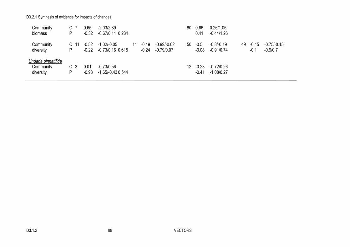
D3.2.1 Synthesis of evidence for impacts of changes  

D3.1.2 88 VECTORS

Community C 7 0.65 -2.03/2.89 80 0.66 0.26/1.05 biomass P -0.32 -0.67/0.11 0.234 0.41 -0.44/1.26 Community C 11 -0.52 -1.02/-0.05 11 -0.49 -0.99/-0.02 50 -0.5 -0.8/-0.19 49 -0.45 -0.75/-0.15 diversity P -0.22 -0.73/0.16 0.615 -0.24 -0.79/0.07 -0.08 -0.91/0.74 -0.1 -0.9/0.7 Undaria pinnatifida Community C 3 0.01 -0.73/0.56 12 -0.23 -0.72/0.26 diversity P -0.98 -1.65/-0.43 0.544 -0.41 -1.08/0.27

D3.2.1 Synthesis of evidence for impacts of changes  

D3.1.2 89 VECTORS

Resampled thoroughly Raw data model Analysis N Median CI PB n Mean CI PB Caulerpa racemosa Species C 8 0.12 -0.72/1.06 116 0.11 -0.14/0.36 abundance P -1.18 -2.7/0.58 0.51 -0.88 -1.34/-0.41 *** Caulerpa taxifolia Species C 10 0.38 -0.26/1.05 84 -0.26 -0.53/0.01 abundance P -0.91 -1.18/0.01 0.318 -0.52 -1.49/0.45 Species C 5 -0.62 -1.73/0.18 37 -0.42 -0.71/-0.14 biomass P 0.1 -0.46/0.7 0.647 0.17 -0.44/0.78 Codium fragile spp. Species C 10 -0.14 -1.11/0.55 84 -0.15 -0.42/0.12 abundance P -0.44 -1.43/0.64 0.528 0.15 -0.39/0.7 Species C 4 7.49 -4.31/7.49 15 1.66 -2.03/5.34 biomass P -0.49 -1.27/-0.01 0.316 -0.53 -4.65/3.59 Species C 7 0.53 -1.78/3.77 33 0.54 -0.39/1.47 growth P -0.1 -0.38/-0.01 0.713 0.04 -2.31/2.39 Sargassum muticum Species C 12 -0.06 -0.79/0.86 176 -0.04 -0.22/0.15 abundance P -0.28 -0.75/0.33 0.6 -0.19 -0.54/0.17

Table 9. Summary of mixed-effect models estimating effect sizes at the species level and testing for differences between consumers (C) and primary producers (P) by invasive species. Effect sizes (“Median” and “95% CI”) and differences between them (PB) were estimated based on 10000 bootstrap samples generated by resampling with replacement (N number of studies included) or based on raw data (n number of data rows included). * P<0.05, ** P<0.01, *** P<0.001

D3.2.1 Synthesis of evidence for impacts of changes  

D3.1.2 90 VECTORS

Resampled thoroughly Resampled thoroughly Raw data model Raw data model bias corrected bias corrected Analysis N Median CI PB N Median CI PB n Mean CI PB n Mean CI PB Intertidal rocky bottom Community C 11 -0.24 -0.94/0.66 164 -0.31 -0.49/-0.12 abundance P -0.68 -1.62/0.01 0.582 -0.34 -0.67/-0.003 Community C 9 -1.56 -2.45/-1.02 9 -1.52 -2.23/-1.02 59 -0.92 -1.42/0.42 58 -0.84 -1.33/-0.34 diversity P -0.06 -0.69/0.55 0.089 -0.09 -0.72/0.51 0.14 -0.5/0.79 ** 0.14 -0.49/0.77 ** Subtidal rocky bottom Community C 23 0.12 -0.34/0.65 23 0.1 -0.36/0.64 199 0.19 -0.18/0.56 184 0.17 -0.16/0.51 abundance P -1.5 -2.43/0.71 0.071 -1.29 -2.01/-0.64 -1.04 -1.49/-0.59 *** -0.81 -1.23/-0.40*** Community C 20 0.04 -0.61/0.7 19 0.04 -0.61/0.7 76 -0.07 -0.59/0.46 55 -0.06 -0.48/0.36 diversity P -2.77 -3.75/-2.07 0.003 -1.69 -2.13/-1.33 ** -2.58 -3.29/-1.85 *** -1.19 -1.84/-0.54 *** Community C 4 -1.0 -1.56/-0.08 12 -0.64 -1.66/0.37 evenness P 0.23 -0.71/0.32 0.779 0.06 -1.54/1.66

Table 10. Summary of mixed-effect models estimating effect sizes at the community level and testing for differences between consumers (C) and primary producers (P) by habitat type. Effect sizes (“Median” and “95% CI”) and differences between them (PB) were estimated based on 10000 bootstrap samples generated by resampling with replacement (N number of studies included) or based on raw data (n number of data rows included). In the case of community abundance and diversity, analyses were re-run on bias-corrected datasets, when this was possible after data elimination. * P<0.05, ** P<0.01, *** P<0.001

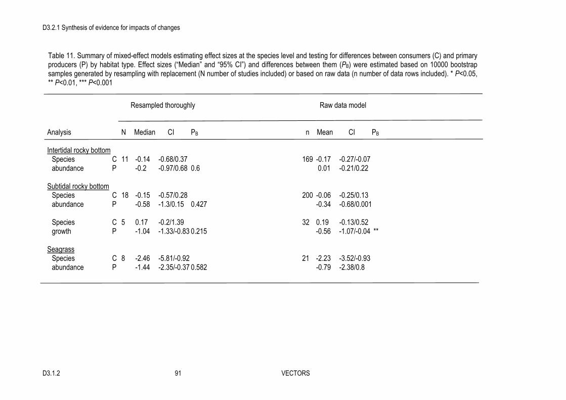
D3.2.1 Synthesis of evidence for impacts of changes  

D3.1.2 91 VECTORS

Resampled thoroughly Raw data model Analysis N Median CI PB n Mean CI PB Intertidal rocky bottom Species C 11 -0.14 -0.68/0.37 169 -0.17 -0.27/-0.07 abundance P -0.2 -0.97/0.68 0.6 0.01 -0.21/0.22 Subtidal rocky bottom Species C 18 -0.15 -0.57/0.28 200 -0.06 -0.25/0.13 abundance P -0.58 -1.3/0.15 0.427 -0.34 -0.68/0.001 Species C 5 0.17 -0.2/1.39 32 0.19 -0.13/0.52 growth P -1.04 -1.33/-0.83 0.215 -0.56 -1.07/-0.04 ** Seagrass Species C 8 -2.46 -5.81/-0.92 21 -2.23 -3.52/-0.93 abundance P -1.44 -2.35/-0.37 0.582 -0.79 -2.38/0.8

Table 11. Summary of mixed-effect models estimating effect sizes at the species level and testing for differences between consumers (C) and primary producers (P) by habitat type. Effect sizes (“Median” and “95% CI”) and differences between them (PB) were estimated based on 10000 bootstrap samples generated by resampling with replacement (N number of studies included) or based on raw data (n number of data rows included). * P<0.05, ** P<0.01, *** P<0.001

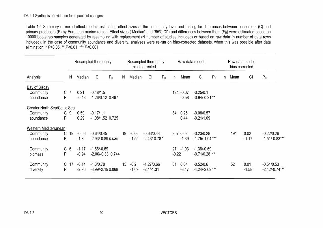
D3.2.1 Synthesis of evidence for impacts of changes  

D3.1.2 92 VECTORS

Resampled thoroughly Resampled thoroughly Raw data model Raw data model bias corrected bias corrected Analysis N Median CI PB N Median CI PB n Mean CI PB n Mean CI PB Bay of Biscay Community C 7 0.21 -0.48/1.5 124 -0.07 -0.25/0.1 abundance P -0.43 -1.26/0.12 0.497 -0.58 -0.94/-0.21 ** Greater North Sea/Celtic Sea Community C 9 0.59 -0.17/1.1 84 0.25 -0.08/0.57 abundance P 0.29 -1.08/1.52 0.725 0.44 -0.21/1.09 Western Mediterranean Community C 19 -0.06 -0.64/0.45 19 -0.06 -0.63/0.44 207 0.02 -0.23/0.28 191 0.02 -0.22/0.26 abundance P -1.8 -2.93/-0.89 0.036 -1.55 -2.43/-0.78 * -1.39 -1.75/-1.04 *** -1.17 -1.51/-0.83*** Community C 6 -1.17 -1.66/-0.69 27 -1.03 -1.38/-0.69 biomass P -0.94 -2.06/-0.33 0.744 -0.22 -0.71/0.28 ** Community C 17 -0.14 -1.3/0.78 15 -0.2 -1.27/0.66 81 0.04 -0.52/0.6 52 0.01 -0.51/0.53 diversity P -2.96 -3.99/-2.19 0.068 -1.69 -2.1/-1.31 -3.47 -4.24/-2.69 *** -1.58 -2.42/-0.74***

Table 12. Summary of mixed-effect models estimating effect sizes at the community level and testing for differences between consumers (C) and primary producers (P) by European marine region. Effect sizes (“Median” and “95% CI”) and differences between them (PB) were estimated based on 10000 bootstrap samples generated by resampling with replacement (N number of studies included) or based on raw data (n number of data rows included). In the case of community abundance and diversity, analyses were re-run on bias-corrected datasets, when this was possible after data elimination. * P<0.05, ** P<0.01, *** P<0.001

D3.2.1 Synthesis of evidence for impacts of changes  

D3.1.2 93 VECTORS

Resampled thoroughly Raw data model Analysis N Median CI PB n Mean CI PB Bay of Biscay Species C 7 -0.28 -1.17/1.21 131 -0.09 -0.24/0.05 abundance P -0.02 -0.62/1.09 0.54 0.04 -0.29/0.38 Greater North Sea Species C 5 -1.0 -1.76/-0.02 66 -0.77 -1.03/-0.51 abundance P -0.05 -0.96/1.75 0.409 -0.11 -0.57/0.35 ** Western Mediterranean Species C 13 -0.16 -1.55/0.43 142 -0.005 -0.31/0.3 abundance P -1.39 -2.52/-0.27 0.511 -1.16 -1.65/-0.68 *** Species C 5 -0.48 -0.48/-0.4 13 -0.22 -1.12/0.67 growth P -0.47 -0.58/-0.32 0.933 -0.66 -1.65/0.34

Table 13. Summary of mixed-effect models estimating effect sizes at the species level and testing for differences between consumers (C) and primary producers (P) by European marine region. Effect sizes (“Median” and “95% CI”) and differences between them (PB) were estimated based on 10000 bootstrap samples generated by resampling with replacement (N number of studies included) or based on raw data (n number of data rows included). * P<0.05, ** P<0.01, *** P<0.001

D3.2.1 Synthesis of evidence for impacts of changes  

D3.1.2 94 VECTORS

Table 14. Results of rank correlation tests for the asymmetry of the funnel plots from the global analysis of community abundance, biomass, diversity and evenness and species abundance, biomass, size and survival.

Response variable Kendall’s τ p

Community abundance -0.21 < 0.0001

Community biomass 0.01 0.789

Community diversity -0.34 < 0.01

Community evenness 0.004 1.000

Species abundance 0.01 0.831

Species biomass -0.00 0.956

Species growth -0.04 0.533

Species survival 0.14 0.129

D3.2.1 Synthesis of evidence for impacts of changes  

D3.1.2 95 VECTORS

Resampled thoroughly Resampled thoroughly Raw data model Raw data model bias corrected bias corrected Analysis N Median CI P N Median CI P n Mean CI P n Mean CI P All studies Community Intercept 53 -0.69 -1.21/-0.17 53 -0.62 -1.11/-0.13 614 -0.68 -0.87/-0.5 594 -0.54 -0.72/-0.36 abundance Slope 0.01 -0.01/0.03 0.405 0.01 -0.08/0.03 0.01 0.01/0.02 *** 0.01 0.01/0.02 *** Community Intercept 21 -0.34 -0.84/0.04 167 -0.04 -0.26/0.33 biomass Slope -0.0004 -0.02/0.01 0.627 -0.004 -0.01/0.005 Community Intercept 44 -1.28 -1.73/-0.89 42 -0.99 -1.33/-0.65 241 -1.32 -1.62/1.02 207 -0.67 -0.97/-0.38 diversity Slope 0.02 0.003/0.03 0.25 0.02 0.003/0.03 0.03 0.02/0.04 *** 0.02 0.01/0.03 *** Community Intercept 6 0.36 -0.11/0.93 20 0.74 -0.39/1.87 evenness Slope -0.04 -0.09/0.06 0.362 -0.03 -0.09/0.03 Experimental studies Community Intercept 22 -0.71 -1.28/-0.05 159 -0.51 -0.8/-0.23 abundance Slope 0.01 -0.02/0.04 0.576 0.01 0.001/0.02 * Community Intercept 7 -0.27 -0.59/0.01 51 -0.17 -0.49/0.15 biomass Slope -0.02 -0.03/0.001 0.217 -0.003 -0.01/0.01 Community Intercept 16 -0.97 -1.23/-0.7 42 -0.85 -1.24/-0.45 diversity Slope 0.01 0.01/0.03 0.563 0.03 0.003/0.05 *

Table 15. Summary of the regressions of effect size on community variables (including both primary producers and consumers)against Halpern’s index for the entire dataset (‘All’) or only for experimental studies. Effect sizes (“Median” and “95% CI”) were estimated based on 10000 bootstrap samples generated by resampling with replacement (N number of studies included) or based on raw data (n number of data rows included). In the case of community abundance and diversity, analyses were re-run on bias-corrected datasets. * P<0.05, ** P<0.01, *** P<0.001

D3.2.1 Synthesis of evidence for impacts of changes  

D3.1.2 96 VECTORS

Resampled thoroughly Resampled thoroughly Raw data model Raw data model bias corrected bias corrected Analysis N Median CI P N Median CI P n Mean CI P n Mean CI P Primary producers Community Intercept 24 -1.09 -1.97/-0.24 24 -0.94 -1.74/-0.18 217 -0.09 -1.39/-0.79 202 -0.85 -1.12/-0.57 abundance Slope -0.001 -0.03/0.03 0.653 -0.002 -0.03/0.02 0.01 -0.001/0.02 -0.01 -0.004/0.02 Community Intercept 18 -0.38 -0.68/-0.08 91 -0.56 -0.84/-0.27 biomass Slope 0.001 -0.01/0.01 0.697 0.01 -0.01/0.02 *** Community Intercept 21 -2.15 -2.85/-1.58 19 -1.48 -1.87/-1.11 98 -2.37 -2.84/-1.91 69 -1.02 -1.4/-0.63 diversity Slope 0.03 0.003/0.05 0.295 0.03 0.01/0.04 0.05 0.03/0.06 *** 0.03 0.02/0.04 *** Consumers Community Intercept 32 -0.25 -0.83/0.34 32 -0.22 -0.79/0.36 397 -0.35 -0.61/-0.1 392 -0.27 -0.52/-0.02 abundance Slope 0.01 -0.01/0.03 0.508 0.01 -0.01/0.03 0.01 0.002/0.02 * 0.01 -0.0004/0.02 Community Intercept 6 0.29 -1.63/1.53 76 1.54 0.99/2.08 biomass Slope -0.03 -0.06/0.02 0.219 -0.04 -0.06/-0.03 *** Community Intercept 26 -0.4 -0.92/0.08 26 -0.37 -0.86/0.1 143 -0.47 -0.88/-0.06 138 -0.37 -0.77/0.04 diversity Slope 0.001 -0.02/0.02 0.695 -0.0001 -0.02/0.02 0.01 -0.002/0.03 0.01 -0.005/0.02

Table 16. Summary of the regressions of effect size on community variables against Halpern’s index for primary producers or consumers. Effect sizes (“Median” and “95% CI”) were estimated based on 10000 bootstrap samples generated by resampling with replacement (N number of studies included) or based on raw data (n number of data rows included). In the case community abundance and diversity, analyses were re-run on bias-corrected datasets. * P<0.05, ** P<0.01, *** P<0.001.

D3.2.1 Synthesis of evidence for impacts of changes  

D3.1.2 97 VECTORS

Resampled thoroughly Raw data model Analysis N Median CI P n Mean CI P All studies Species Intercept 46 -0.78 -1.5/-0.13 558 -0.62 -0.76/-0.48 abundance Slope 0.02 -0.003/0.04 0.25 0.01 0.01/0.02 *** Species Intercept 13 0.02 -0.85/0.53 169 -0.15 -0.4/0.1 biomass Slope -0.01 -0.04/0.01 0.512 -0.003 -0.01/0.01 Species Intercept 16 -1.24 -2.62/0.58 88 -0.42 -1.09/0.26 growth Slope 0.04 -0.002/0.08 0.551 0.01 -0.02/0.04 Species Intercept 9 -1.35 -2.19/-0.6 43 -0.79 -1.48/-0.09 survival Slope 0.002 -0.03/0.05 0.79 0.02 -0.01/0.04 Experimental studies Species Intercept 22 -0.47 -1.2/0.27 140 -0.38 -0.64/-0.12 abundance Slope 0.003 -0.02/0.03 0.567 0.01 -0.01/0.02 Species Intercept 6 -0.44 -0.98/0.02 81 -0.63 -0.78/-0.48 biomass Slope -0.003 -0.03/0.02 0.738 -0.002 -0.005/0.01 Species Intercept 12 -1.16 -2.7/1.13 63 -0.48 -1.43/0.47 growth Slope 0.04 -0.01/0.08 0.641 0.02 -0.03/0.06 Species Intercept 7 -0.57 -1.49/0.29 40 -0.61 -1.35/0.13 survival Slope -0.02 -0.06/0.03 0.725 0.01 -0.01/0.04

Table 17. Summary of the regressions of effect size on species variables (including both primary producers and consumers)against Halpern’s index for the entire dataset (‘All’) or only for experimental studies. Effect sizes (“Median” and “95% CI”) were estimated based on 10000 bootstrap samples generated by resampling with replacement (N number of studies included) or based on raw data (n number of data rows included). * P<0.05, ** P<0.01, *** P<0.001

D3.2.1 Synthesis of evidence for impacts of changes  

D3.1.2 98 VECTORS

Resampled thoroughly Raw data model Analysis N Median CI P n Mean CI P Primary producers Species Intercept 23 -0.3 -1.18/0.65 125 -0.71 -0.98/-0.45 abundance Slope -0.01 -0.04/0.02 0.528 0.01 0.002/0.02 * Species Intercept 9 -0.06 -0.45/0.33 91 -0.34 -0.62/-0.06 biomass Slope -0.01 -0.04/0.004 0.553 -0.005 -0.005/0.01 Species Intercept 8 -2.18 -2.66/-1.75 53 -0.71 -1.19/0.24 growth Slope 0.09 0.06/0.11 0.085 0.01 -0.01/0.03 Consumers Species Intercept 29 -0.94 -1.78/-0.34 433 -0.56 -0.74/-0.39 abundance Slope 0.03 0.01/0.06 0.037 0.01 0.01/0.02 *** Species Intercept 4 1.02 -3.36/2.62 78 0.41 -0.08/0.9 biomass Slope -0.03 -0.08/0.08 0.635 -0.02 -0.03/-0.01 ** Species Intercept 8 -0.2 -3.94/5.82 35 -0.05 -1.42/1.32 growth Slope -0.01 -0.16/0.1 0.611 0.003 -0.06/0.07 Species Intercept 7 -0.57 -1.49/0.29 40 -0.61 -1.35/0.13 survival Slope -0.02 -0.06/0.03 0.725 0.01 -0.01/0.04

Table 18. Summary of the regressions of effect size on species variables against Halpern’s index for primary producers or consumers. Effect sizes (“Median” and “95% CI”) were estimated based on 10000 bootstrap samples generated by resampling with replacement (N number of studies included) or based on raw data (n number of data rows included). In both cases, analyses were re-run on bias-corrected datasets. * P<0.05, ** P<0.01, *** P<0.001

D3.2.1 Synthesis of evidence for impacts of changes  

D3.1.2 99 VECTORS

Figure 1. Example of a graph representing the null (blue) and the observed (red) distributions, the critical value at which α is = 0.05 (dotted line) and the median QM (red line)

D3.2.1 Synthesis of evidence for impacts of changes  

D3.1.2 100 VECTORS

Figure 2. Geographical distribution of the retained studies.

D3.2.1 Synthesis of evidence for impacts of changes  

D3.1.2 101 VECTORS

-2

-1

0

1

2

Primary producersConsumers

P = 0.121P =0.014

A) Community abundance

-3

-2

-1

0

1

2

3

Effe

ct S

ize

P = 0.573

B) Community biomass

-3

-2

-1

0

1

2

3

P = 0.023

C) Community diversity

P = 0.056

-3

-2

-1

0

1

2

3

P = 0.505

D) Community evenness

All data Experimental data All data

N = 53 N = 22

N = 44 N = 16

N = 21

N = 7

Figure 3. Effects of exotic seaweeds on A) abundance, B) biomass, C) diversity and D) evenness of communities of primary producers and consumers, calculated using all data or experimental data only. Symbols report median effect size calculated using 10000 bootstrap samples and 95% confidence intervals. Probabilities refer to the comparison of effects sizes between primary producers and consumers for All data and experimental data separately. NS, not significant.

D3.2.1 Synthesis of evidence for impacts of changes  

D3.1.2 102 VECTORS

-2

-1

0

1

2

Primary producersConsumers

P = 0.517

A) Species abundance

P = 0.296

-4

-2

0

2

4

P = 0.260

B) Species biomass

P = 0.274

-2

-1

0

1

2

P = 0.582

C) Species growth

P = 0.626

-3

-2

-1

0

1

2

3

P = 0.617

All data Experimental data

D) Species survival

P = 0.488

Effe

ct s

ize

All data Experimental data

N=46 N=22 N=17 N=10

N=18 N=14 N=13 N=11

Figure 4. Effects of exotic seaweeds on A) abundance, B) biomass, C) growth and D) survival of primary producer and consumer species, calculated using all data or experimental data only. Symbols report median effect size calculated using 10000 bootstrap samples and 95% confidence intervals. Probabilities refer to the comparison of effects sizes between primary producers and consumers for All data and experimental data separately.

D3.2.1 Synthesis of evidence for impacts of changes  

D3.1.2 103 VECTORS

A) Community abundance

-4

-2

0

2

4Primary producersConsumers

Codium spp. C. racemosa C. taxifolia S. muticum

P = 0.412 P = 0.534 P = 0.221P = 0.043

U. pinnatifida

B) Community biomass

-4

-2

0

2

4

C) Community diversity

Effe

ct S

ize

-6

-4

-2

0

2

4

6

P = 0.594 P = 0.563 P = 0.544P = 0.012 P = 0.615

P = 0.2234

N=7 N=17 N=11 N=15

N=7

N=6 N=14 N=9 N=11 N=3

Figure 5. Effects of different exotic seaweeds on A) abundance, B) biomass and C) diversity of communities of primary producers and consumers. Symbols report median effect size calculated using 10000 bootstrap samples and 95% confidence intervals. Probabilities refer to the comparison of effects sizes between primary producers and consumers for All data and experimental data separately.

D3.2.1 Synthesis of evidence for impacts of changes  

D3.1.2 104 VECTORS

A) Species abundance

-3

-2

-1

0

1

2

3Primary producersConsumers

P = 0.528 P = 0.318 P = 0.6P = 0.51

B) Species biomass

Effe

ct S

ize

-15

-10

-5

0

5

10

15

P = 0.316 P = 0.647

C) Species growth

-15

-10

-5

0

5

10

15

Codium spp. C. racemosa C. taxifolia S. muticum

P = 0.713

N=10 N=8 N=10 N=12

N=4 N=5

N=7

Figure 6. Effects of different exotic seaweeds on A) abundance, B) biomass and C) growth of primary producer and consumer species. Symbols report median effect size calculated using 10000 bootstrap samples and 95% confidence intervals. Probabilities refer to the comparison of effects sizes between primary producers and consumers for All data and experimental data separately.

D3.2.1 Synthesis of evidence for impacts of changes  

D3.1.2 105 VECTORS

B) Community diversity

-4

-3

-2

-1

0

1

2

3

4

P = 0.89 P = 0.003

A) Community abundance

-3

-2

-1

0

1

2

3 Primary producersConsumers

P = 0.582

C) Community evenness

-2

-1

0

1

2

Intertidal rocky bottoms Subtidal rocky bottoms

Effe

ct S

ize

P = 0.071

P = 0.779

N=11 N=23

N=9 N=20

N=4

Figure 7. Effects of different exotic seaweeds on A) abundance, B) biomass and C) evenness of communities of primary producers and consumers. Symbols report median effect size calculated using 10000 bootstrap samples and 95% confidence intervals. Probabilities refer to the comparison of effects sizes between primary producers and consumers for All data and experimental data separately.

D3.2.1 Synthesis of evidence for impacts of changes  

D3.1.2 106 VECTORS

A) Species abundance

-6

-4

-2

0

2

4

6 Primary producersConsumers

P = 0.6 P = 0.582P = 0.427

B) Species growth

-2

-1

0

1

2

Intertidal rocky bottoms Subtidal rocky bottoms Seagrass beds

P = 0.215

N=11 N=18 N=8

N=5

Figure 8. Effects of different exotic seaweeds on A) abundance and B) growth of primary producer and consumer species. Symbols report median effect size calculated using 10000 bootstrap samples and 95% confidence intervals. Probabilities refer to the comparison of effects sizes between primary producers and consumers for All data and experimental data separately.

D3.2.1 Synthesis of evidence for impacts of changes  

D3.1.2 107 VECTORS

-4

-2

0

2

4

Primary producersConsumers

A) Community abundance

P = 0.497 P = 0.725 P = 0.036

-4

-2

0

2

4 B) Community biomass

P = 0.744

-4

-2

0

2

4 C) Community diversity

Bay of Biscay Greater North Sea Western Mediterranean

P = 0.068

N=7 N=9 N=19

N=6

N=17

Fig 9. Effects of exotic seaweeds on A) abundance, B) biomass and C) diversity of communities of primary producers and consumers in different European regional seas. Symbols report median effect size calculated using 10000 bootstrap samples and 95% confidence intervals. Probabilities refer to the comparison of effects sizes between primary producers and consumers for All data and experimental data separately.

D3.2.1 Synthesis of evidence for impacts of changes  

D3.1.2 108 VECTORS

-4

-2

0

2

4

Primary producersConsumers

A) Species abundance

P = 0.54 P =0.409 P = 0.54

-1.0

-0.5

0.0

0.5

1.0 B) Species size

Bay of Biscay Greater North Sea Western Mediterranean

P = 0.933

N=7 N=5 N=13

N=5

Figure 10. Effects of exotic seaweeds on A) abundance and B) growth of primary producer and consumer species in different European regional seas. Symbols report median effect size calculated using 10000 bootstrap samples and 95% confidence intervals. Probabilities refer to the comparison of effects sizes between primary producers and consumers for All data and experimental data separately.

D3.2.1 Synthesis of evidence for impacts of changes  

D3.1.2 109 VECTORS

B) Community biomass

A) Community abundance

D) Community evenness

C) Community diversity

Figure 11. Funnel plots for community A) abundance, B) biomass, C) diversity and D) evenness. Data included in squares represent those that have been removed to correct for publication bias.

D3.2.1 Synthesis of evidence for impacts of changes  

D3.1.2 110 VECTORS

B) Species biomass A) Species abundance

C) Species growth D) Species survival

Figure 12. Funnel plots for species A) abundance, B) biomass, C) growth and D) survival.

D3.2.1 Synthesis of evidence for impacts of changes  

D3.1.2 111 VECTORS

A) All data B) Experimental data

C) Primary producers

Halpern index Halpern index

Halpern index

Effe

ct s

ize

Effe

ct s

ize

Figure 13. Regression of effect size on community diversity against Halpern’s index for A) all data, B) experimental data and C) primary producers.

D3.2.1 Synthesis of evidence for impacts of changes  

D3.1.2 112 VECTORS

Effe

ct s

ize

Halpern index

Figure 14. Regression of effect size on consumer species abundance against Halpern’s index.

D3.2.1 Synthesis of evidence for impacts of changes  

D3.1.2 113 VECTORS

Annex A. Search terms used to find relevant studies

We searched for relevant studies in Web of Science online database using a complex set of search terms:

(alga* OR macroalga* OR seaweed*) AND (alien*OR invasi*OR introduced OR allochthonous OR nonindigenous OR non-indigenous OR “non native*” OR non-native* OR exotic*) AND (marine OR brackish OR estuar*OR coastal OR shallow OR sea*OR aquatic OR maritime OR lagoon* OR pelagic OR benth* OR demersal OR shore* OR intertidal OR subtidal OR ocean* OR bay OR cove) AND (impact* OR effect* OR influence OR consequence* OR food-web* OR “food web*” OR ecosystem* OR biomass OR biodiversity OR “biological diversity” OR communit* OR richness OR diversity OR abundance OR evenness OR cover OR density OR “reproductive capacity” OR mortality OR growth OR assemblage* OR producti* OR decomposition OR “nutrient cycl*” OR oxygen OR carbon OR flux OR respiration OR “ecosystem metabolism” OR “sediment stabilisation” OR epiphyte* OR “sediment mixing” OR resilience OR stability OR resistance OR invasibility).

Annex B. List of papers reviewed (data extracted from these papers have been archived and available as part of VECTORS Deliverable 3.1.1)

Ambrose RF, Nelson BV (1982) Inhibition of giant kelp recruitment by an introduced brown alga. Botanica Marina 25: 265-267 Balata D, Piazzi L, Cinelli F (2004) A comparison among assemblages in areas invaded by Caulerpa taxifolia and C. racemosa on a subtidal Mediterranean rocky bottom. Marine Ecology-Pubblicazioni Della Stazione Zoologica Di Napoli I 25: 1-13 Baldacconi R, CORriero G (2009) Effects of the spread of the alga Caulerpa racemosa var. cylindracea on the sponge assemblage from coralligenous concretions of the Apulian coast (Ionian Sea, Italy). Marine Ecology-an Evolutionary Perspective 30: 337-345 Ballesteros E, Cebrian E, Alcoverro T (2007) Mortality of shoots of Posidonia oceanica following meadow invasion by the red alga Lophociadia lallemandii. Botanica Marina 50: 8-13 Bartoli P, Boudouresque CF (1997) Transmission failure of parasites (Digenea) in sites colonized by the recently introduced invasive alga Caulerpa taxifolia. Marine Ecology-Progress Series 154: 253-260 Boudouresque CF, Lemée R, Mari X, Meinesz A (1996) The invasive alga Caulerpa taxifolia is not a suitable diet for the sea urchin Paracentrotus lividus. Aquatic Botany 53: 245-250 Box A, Sureda A, Deudero S (2008) Antioxidant response of the bivalve Pinna nobilis colonised by invasive red macroalgae Lophocladia lallemandii. Comparative Biochemistry and Physiology C-Toxicology & Pharmacology 149: 456-460 Box A, Sureda A, Deudero S, Blanco A, Terrados J, Grau AM, Riera F (2009) Diet and physiological responses of Spondyliosoma cantharus (Linnaeus, 1758) to the Caulerpa racemosa var. cylindracea invasion. Journal of Experimental Marine Biology and Ecology 380: 11-19

D3.2.1 Synthesis of evidence for impacts of changes  

D3.1.2 114 VECTORS

Britton-Simmons KH (2004) Direct and indirect effects of the introduced alga Sargassum muticum on benthic, subtidal communities of Washington State, USA. Marine Ecology-Progress Series 277: 61-78 Britton-Simmons KH, Pister B, Sanchez I, Okamoto D (2011) Response of a native, herbivorous snail to the introduced seaweed Sargassum muticum. Hydrobiologia 661: 187-196 Bulleri F, Airoldi L, Branca GM, Abbiati M (2006) Positive effects of the introduced green alga, Codium fragile ssp. tomentosoides, on recruitment and survival of mussels. Marine Biology 148: 1213-1220 Bulleri F, Balata D, Bertocci I, Tamburello L, Benedetti-Cecchi L (2010) The seaweed Caulerpa racemosa on Mediterranean rocky reefs: from passenger to driver of ecological change. Ecology 91: 2205-2212 Buschbaum C, Chapman AS, Saier B (2006) How an introduced seaweed can affect epibiota diversity in different coastal systems. Marine Biology 148: 743-754 Byers JE, Wright JT, Gribben PE (2010) Variable direct and indirect effects of a habitat-modifying invasive species on mORtality of native fauna. Ecology 91: 1787-1798 Cacabelos E, Olabarria C, Incera M, Troncoso JS (2010) Effects of habitat structure and tidal height on epifaunal assemblages associated with macroalgae. Estuarine Coastal and Shelf Science 89: 43-52 Carroll JM, Peterson BJ, Bonal D, Weinstock A, Smith CF, Tettelbach ST (2010) Comparative survival of bay scallops in eelgrass and the introduced alga, Codium fragile, in a New York estuary. Marine Biology 157: 249-259 Casas G, Scrosati R, Piriz ML (2004) The invasive kelp Undaria pinnatifida (Phaeophyceae, Laminariales) reduces native seaweed diversity in Nuevo Gulf (Patagonia, Argentina). Biological Invasions 6: 411-416 Ceccherelli G, Campo D (2002) Different effects of Caulerpa racemosa on two co-occurring seagrasses in the Mediterranean. Botanica Marina 45: 71-76 Ceccherelli G, Sechi N (2002) Nutrient availability in the sediment and the reciprocal effects between the native seagrass Cymodocea nodosa and the introduced rhizophytic alga Caulerpa taxifolia. Hydrobiologia 474: 57-66 Chavanich S, Harris LG (2004) Impact of the non-native macroalga Codium fragile (Sur.) Hariot ssp tomentosoides (van Goor) Silva on the native snail Lacuna vincta (Montagu, 1803) in the Gulf of Maine. Veliger 47: 85-90 Chrisholm JRM, Moulin P (2003) Stimulation of nitrogen fixation in refractory organic sediments by Caulerpa taxifolia (Chlorophyta). Limnology and Oceanography 48: 787-794 Curiel D, Guidetti P, Bellemo G, Scattolin M, Marzocchi M (2002) The introduced alga Undaria pinnatifida (Laminariales, Alariaceae) in the lagoon of Venice. Hydrobiologia 477: 209-219 Deudero S, Blanco A, Box A, Mateu-Vicens G, Cabanellas-Reboredo M, Sureda A (2010) Interaction between the invasive macroalga Lophocladia lallemandii and the bryozoan Reteporella grimaldii at seagrass meadows: density and physiological responses. Biological Invasions 12: 41-52

D3.2.1 Synthesis of evidence for impacts of changes  

D3.1.2 115 VECTORS

Deudero S, Box A, Alos J, Arroyo NL, Marba N (2011) Functional changes due to invasive species: Food web shifts at shallow Posidonia oceanica seagrass beds colonized by the alien macroalga Caulerpa racemosa. Estuarine Coastal and Shelf Science 93: 106-116 Devillele X, Verlaque M (1995) Changes and degradation in a Posidonia oceanica bed invaded by the introduced tropical alga Caulerpa taxifolia in the North-Western Mediterranean. Botanica Marina 38: 79-87 Drouin A, McKindsey CW, Johnson LE (2011) Higher abundance and diversity in faunal assemblages with the invasion of Codium fragile ssp fragile in eelgrass meadows. Marine Ecology-Progress Series 424: 105-117 Drouin A, McKindsey CW, Johnson LE (2012) Detecting the impacts of notorious invaders: experiments versus observations in the invasion of eelgrass meadows by the green seaweed Codium fragile. Oecologia 168: 491-502 Dumay O, Fernandez C, Pergent G (2002) Primary production and vegetative cycle in Posidonia oceanica when in competition with the green algae Caulerpa taxifolia and Caulerpa racemosa. Journal of the Marine Biological Association of the United Kingdom 82: 379-387 Dumay O, Costa J, Desjobert JM, Pergent G (2004) Variations in the concentration of phenolic compounds in the seagrass Posidonia oceanica under conditions of competition. Phytochemistry 65: 3211-3220 Eyre BD, Maher D, Oakes JM, Erler DV, Glasby TM (2011) Differences in benthic metabolism, nutrient fluxes, and denitrification in Caulerpa taxifolia communities compared to uninvaded bare sediment and seagrass (Zostera capricorni) habitats. Limnology and Oceanography 56: 1737-1750 Ferrer E, Garreta AG, Ribera MA (1997) Effect of Caulerpa taxifolia on the productivity of two Mediterranean macrophytes. Marine Ecology-Progress Series 149: 279-287 Francour P, Harmelin-Vivien M, Harmelin JG, Duclerc J (1995) Impact of Caulerpa taxifolia colonization on the ichthyofauna of North-Western Mediterranean Sea – Preliminary results. Hydrobiologia 300: 345-353 Francour P, Pellissier V, Mangialajo L, Buisson E, Stadelmann B, Veillard N, Meinesz A, Thibaut T, De Vaugelas J (2009) Changes in invertebrate assemblages of Posidonia oceanica beds following Caulerpa taxifolia invasion. Vie et Milieu – Life and Environment 59: 31-38 Gallucci F, Hutchings P, Gribben P, Fonseca G (2012) Habitat alteration and community-level effects of an invasive ecosystem engineer: a case study along the coast of NSW, Australia. Marine Ecology-Progress Series 449: 95-108 Gennaro P, Piazzi L (2011) Synergism between two anthropic impacts: Caulerpa racemosa var. cylindracea invasion and seawater nutrient enrichment. Marine Ecology-Progress Series 427: 59-70 Gestoso I, Olabarria C, Troncoso JS (2010) Variability of epifaunal assemblages associated with native and invasive macroalgae. Marine and Freshwater Research 61: 724-731

D3.2.1 Synthesis of evidence for impacts of changes  

D3.1.2 116 VECTORS

Gollan JR, Wright JT (2006) Limited grazing pressure by native herbivores on the invasive seaweed Caulerpa taxifolia in a temperate Australian estuary. Marine and Freshwater Research 57: 685-694 Gribben PE, Wright JT (2006) Invasive seaweed enhances recruitment of a native bivalve: roles of refuge from predation and the habitat choice of recruits. Marine Ecology-Progress Series 318: 177-185 Gribben PE, Wright JT (2006) Sublethal effects on reproduction in native fauna: are females more vulnerable to biological invasion? Oecologia 149: 352-361 Gribben PE, Wright JT, O'Connor WA, Doblin MA, Eyre B, Steinberg PD (2009) Reduced performance of native infauna following recruitment to a habitat-forming invasive marine alga. Oecologia 158: 733-745 Gribben PE, Wright JT, O'Connor WA, Steinberg P (2009) Larval settlement preference of a native bivalve: the influence of an invasive alga versus native substrata. Aquatic Biology 7: 217-227 Harmelin-Vivien M, Harmelin JG, Francour P (1996) A 3-year study of the littoral fish fauna of sites colonized by Caulerpa taxifolia in the N.W. Medterranean (Menton, France) In: Ribera MA, Ballesteros E, Boudouresque CF, Gomez A, Gravez V (eds) Second International workshop on Caulerpa taxifolia. Publicacions Universitat Barcelona, p 391-397 Harries DB, Harrow S, Wilson JR, Mair JM, Donnan DW (2007) The establishment of the invasive alga Sargassum muticum on the west coast of Scotland: a preliminary assessment of community effects. Journal of the Marine Biological Association of the United Kingdom 87: 1057-1067 Hendriks IE, Bouma TJ, MORris EP, Duarte CM (2010) Effects of seagrasses and algae of the Caulerpa family on hydrodynamics and particle-trapping rates. Marine Biology 157:473-481 Hoffle H, Thomsen MS, Holmer M (2011) High mORtality of Zostera marina under high temperature regimes but minor effects of the invasive macroalgae Gracilaria vermiculophylla. Estuarine Coastal and Shelf Science 92: 35-46 Holmer M, Marba N, Lamote M, Duarte CM (2009) Deterioration of Sediment Quality in Seagrass Meadows (Posidonia oceanica) Invaded by Macroalgae (Caulerpa sp.). Estuaries and Coasts 32: 456-466 Husa V, Sjotun K, BrattenbORg N, Lein TE (2008) Changes of macroalgal biodiversity in sublittoral sites in southwest NORway: impact of an introduced species or higher temperature? Marine Biology Research 4: 414-428 Ingolfsson A (2008) The invasion of the intertidal canopy-forming alga Fucus serratus L. to southwestern Iceland: Possible community effects. Estuarine Coastal and Shelf Science 77: 484-490 Irigoyen AJ, Eyras C, Parma AM (2011) Alien algae Undaria pinnatifida causes habitat loss for rocky reef fishes in north Patagonia. Biological Invasions 13: 17-24 Irigoyen AJ, Trobbiani G, Sgarlatta MP, Raffo MP (2011) Effects of the alien algae Undaria pinnatifida (Phaeophyceae, Laminariales) on the diversity and abundance of benthic macrofauna in Golfo Nuevo (Patagonia, Argentina): potential implications for local food webs. Biological Invasions 13: 1521-1532

D3.2.1 Synthesis of evidence for impacts of changes  

D3.1.2 117 VECTORS

Janiak DS, Whitlatch RB (2012) Epifaunal and algal assemblages associated with the native Chondrus crispus (Stackhouse) and the non-native Grateloupia turuturu (Yamada) in eastern Long Island Sound. Journal of Experimental Marine Biology and Ecology 413: 38-44 Jones E, Thornber CS (2010) Effects of habitat-modifying invasive macroalgae on epiphytic algal communities. Marine Ecology-Progress Series 400: 87-100 Kelly JR, Scheibling RE, Balch T (2011) Invasion-mediated shifts in the macrobenthic assemblage of a rocky subtidal ecosystem. Marine Ecology-Progress Series 437: 69-78 Klein JC, Verlaque M (2011) Experimental removal of the invasive Caulerpa racemosa triggers partial assemblage recovery. Journal of the Marine Biological Association of the United Kingdom 91: 117-125 Lang AC, Buschbaum C (2010) Facilitative effects of introduced Pacific oysters on native macroalgae are limited by a secondary invader, the seaweed Sargassum muticum. Journal of Sea Research 63: 119-128 Lawson SE, McGlathery KJ, Wiberg PL (2012) Enhancement of sediment suspension and nutrient flux by benthic macrophytes at low biomass. Marine Ecology-Progress Series 448: 259-270 Levi F, Francour P (2004) Behavioural response of Mullus surmuletus to habitat modification by the invasive macroalga Caulerpa taxifolia. Journal of Fish Biology 64: 55-64 Levin PS, Coyer JA, Petrik R, Good TP (2002) Community-wide effects of nonindigenous species on temperate rocky reefs. Ecology 83: 3182-3193 Lutz ML, Davis AR, Minchinton TE (2010) Non-indigenous macroalga hosts different epiphytic assemblages to conspecific natives in southeast Australia. Marine Biology 157: 1095-1103 Lyons DA, Scheibling RE (2007) Differences in somatic and gonadic growth of sea urchins (Stronglyocentrotus droebachiensis) fed kelp (Laminaria longicruris) or the invasive alga Codium fragile ssp tomentosoides are related to energy acquisition. Marine Biology 152: 285-295 Lyons DA, Scheibling RE (2007) Effect of dietary history and algal traits on feeding rate and food preference in the green sea urchin Strongylocentrotus droebachiensis. Journal of Experimental Marine Biology and Ecology 349: 194-204 Martinez-Luscher J, Holmer M (2010) Potential effects of the invasive species Gracilaria vermiculophylla on Zostera marina metabolism and survival. Marine Environmental Research 69: 345-349 McKinnon JG, Gribben PE, Davis AR, Jolley DF, Wright JT (2009) Differences in soft-sediment macrobenthic assemblages invaded by Caulerpa taxifolia compared to uninvaded habitats. Marine Ecology-Progress Series 380: 59-71 Molenaar H, Meinesz A, Thibaut T (2009) Alterations of the structure of Posidonia oceanica beds due to the introduced alga Caulerpa taxifolia. Scientia Marina 73: 329-335 Nohren E, Odelgard E (2010) Response of epibenthic faunal assemblages to varying vegetation structures and habitat patch size. Aquatic Biology 9: 139-148

D3.2.1 Synthesis of evidence for impacts of changes  

D3.1.2 118 VECTORS

Olabarria C, Incera M, Garrido J, Rossi F (2010) The effect of wrack composition and diversity on macrofaunal assemblages in intertidal marine sediments. Journal of Experimental Marine Biology and Ecology 396: 18-26 Olabarria C, Rodil IF, Incera M, Troncoso JS (2009) Limited impact of Sargassum muticum on native algal assemblages from rocky intertidal shores. Marine Environmental Research 67: 153-158 Pacciardi L, De Biasi AM, Piazzi L (2011) Effects of Caulerpa racemosa invasion on soft-bottom assemblages in the Western Mediterranean Sea. Biological Invasions 13: 2677-2690 Pederson HG, Johnson CR (2008) Growth and age structure of sea urchins (Heliocidaris erythrogramma) in complex barrens and native macroalgal beds in eastern Tasmania. Ices Journal of Marine Science 65: 1-11 Piazzi L, Balata D (2008) The spread of Caulerpa racemosa var. cylindracea in the Mediterranean Sea: An example of how biological invasions can influence beta diversity. Marine Environmental Research 65: 50-61 Piazzi L, Balata D (2009) Invasion of alien macroalgae in different Mediterranean habitats. Biological Invasions 11: 193-204 Piazzi L, Balata D, Cecchi E, Cinelli F (2003) Co-occurrence of Caulerpa taxifolia and C. racemosa in the Mediterranean Sea: interspecific interactions and influence on native macroalgal assemblages. Cryptogamie Algologie 24: 233-243 Piazzi L, Balata D, Ceccherelli G, Cinelli F (2005) Interactive effect of sedimentation and Caulerpa racemosa var. cylindracea invasion on macroalgal assemblages in the Mediterranean Sea. Estuarine Coastal and Shelf Science 64: 467-474 Piazzi L, Balata D, Cinelli F (2007) Invasions of alien macroalgae in Mediterranean coralligenous assemblages. Cryptogamie Algologie 28: 289-301 Piazzi L, Balata D, Foresi L, Cristaudo C, Cinelli F (2007) Sediment as a constituent of Mediterranean benthic communities dominated by Caulerpa racemosa var. cylindracea. Scientia Marina 71: 129-135 Piazzi L, Ceccherelli G (2006) Persistence of biological invasion effects: Recovery of macroalgal assemblages after removal of Caulerpa racemosa var. cylindracea. Estuarine Coastal and Shelf Science 68: 455-461 Piazzi L, Ceccherelli G, Cinelli F (2001) Threat to macroalgal diversity: effects of the introduced green alga Caulerpa racemosa in the Mediterranean. Marine Ecology-Progress Series 210: 149-159 Piazzi L, Cinelli F (2003) Evaluation of benthic macroalgal invasion in a harbour area of the western Mediterranean Sea. European Journal of Phycology 38: 223-231 Polte P, Buschbaum C (2008) Native pipefish Entelurus aequoreus are promoted by the introduced seaweed Sargassum muticum in the northern Wadden Sea, NORth Sea. Aquatic Biology 3: 11-18 Prado P. Thibaut T (2008) Differences between epiphytic assemblages on introduced Caulerpa taxifolia and coexisting eelgrass (Zostera capricorni) in Botany Bay (NSW, Australia). Scientia Marina 72: 645-654

D3.2.1 Synthesis of evidence for impacts of changes  

D3.1.2 119 VECTORS

Raffo MP, Eyras MC, Iribarne OO (2009) The invasion of Undaria pinnatifida to a Macrocystis pyrifera kelp in Patagonia (Argentina, south-west Atlantic). Journal of the Marine Biological Association of the United Kingdom 89: 1571-1580 Relini G, Relini M, Torchia G (1998) Fish biodiversity in a Caulerpa taxifolia meadow in the Ligurian Sea. Italian Journal of Zoology 65: 465-470 Rodil IF, Olabarria C, Lastra M, Lopez J (2008) Differential effects of native and invasive algal wrack on macrofaunal assemblages inhabiting exposed sandy beaches. Journal of Experimental Marine Biology and Ecology 358: 1-13 Rohr NE, Thornber CS, Jones E (2011) Epiphyte and herbivore interactions impact recruitment in a marine subtidal system. Aquatic Ecology 45: 213-219 Rossi F, Incera M, Callier M, Olabarria C (2011) Effects of detrital non-native and native macroalgae on the nitrogen and carbon cycling in intertidal sediments. Marine Biology 158: 2705-2715 Sanchez I, Fernandez C (2005) Impact of the invasive seaweed Sargassum muticum (Phaeophyta) on an intertidal macroalgal assemblage. Journal of Phycology 41: 923-930 Sanchez I, Fernandez C, Arrontes J (2005) Long-term changes in the structure of intertidal assemblages after invasion by Sargassum muticum (Phaeophyta). Journal of Phycology 41: 942-949 Scheibling RE, Anthony SX (2001) Feeding, growth and reproduction of sea urchins (Strongylocentrotus droebachiensis) on single and mixed diets of kelp (Laminaria spp.) and the invasive alga Codium fragile ssp tomentosoides. Marine Biology 139: 139-146 Scheibling RE, Gagnon P (2006) Competitive interactions between the invasive green alga Codium fragile ssp tomentosoides and native canopy-forming seaweeds in Nova Scotia (Canada). Marine Ecology-Progress Series 325: 1-14 Schmidt AL, Scheibling RE (2006) A comparison of epifauna and epiphytes on native kelps (Laminaria species) and an invasive alga (Codium fragile ssp tomentosoides) in Nova Scotia, Canada. Botanica Marina 49: 315-330 Schmidt AL, Scheibling RE (2007) Effects of native and invasive macroalgal canopies on composition and abundance of mobile benthic macrofauna and turf-forming algae. Journal of Experimental Marine Biology and Ecology 341: 110-130 Siddon CE, Witman JD (2004) BehaviORal indirect interactions: Multiple predator effects and prey switching in the rocky subtidal. Ecology 85: 2938-2945 Staehr PA, Pedersen MF, Thomsen MS, Wernberg T, Krause-Jensen D (2000) Invasion of Sargassum muticum in Limfjorden (Denmark) and its possible impact on the indigenous macroalgal community. Marine Ecology-Progress Series 207: 79-88 Strong JA, Dring MJ (2011) Macroalgal competition and invasive success: testing competition in mixed canopies of Sargassum muticum and Saccharina latissima. Botanica Marina 54: 223-229

D3.2.1 Synthesis of evidence for impacts of changes  

D3.1.2 120 VECTORS

Strong JA, Dring MJ, Maggs CA (2006) Colonisation and modification of soft substratum habitats by the invasive macroalga Sargassum muticum. Marine Ecology-Progress Series 321: 87-97 Strong JA, Maggs CA, Johnson MP (2009) The extent of grazing release from epiphytism for Sargassum muticum (Phaeophyceae) within the invaded range. Journal of the Marine Biological Association of the United Kingdom 89: 303-314 Sureda A, Box A, Deudero S, Pons A (2009) Reciprocal effects of caulerpenyne and intense herbivorism on the antioxidant response of Bittium reticulatum and Caulerpa taxifolia. Ecotoxicology and Environmental Safety 72: 795-801 Sureda A, Box A, Terrados J, Deudero S, Pons A (2008) Antioxidant response of the seagrass Posidonia oceanica when epiphytized by the invasive macroalgae Lophodadia lallemandii. Marine Environmental Research 66: 359-363 Tanner JE (2011) Utilisation of the Invasive Alga Caulerpa taxifolia as Habitat by Faunal Assemblages in the Port River-Barker Inlet Estuary, South Australia. Estuaries and Coasts 34: 831-838 Taylor SL, Bishop MJ, Kelaher BP, Glasby TM (2010) Impacts of detritus from the invasive alga Caulerpa taxifolia on a soft sediment community. Marine Ecology-Progress Series 420: 73-81 Thomsen MS (2010) Experimental evidence for positive effects of invasive seaweed on native invertebrates via habitat-formation in a seagrass bed. Aquatic Invasions 5: 341-346 Tomas F, Box A, Terrados J (2011) Effects of invasive seaweeds on feeding preference and performance of a keystone Mediterranean herbivore. Biological Invasions 13: 1559-1570 Trowbridge CD (2001) Coexistence of introduced and native congeneric algae: Codium fragile and C. tomentosum on Irish rocky intertidal shores. Journal of the Marine Biological Association of the United Kingdom 81:931-937 Trowbridge CD, Todd CD (2001) Host-plant change in marine specialist herbivores: Ascoglossan sea slugs on introduced macroalgae. Ecological Monographs 71: 219-243 Ulas A, Duzbastilar FO, Aydin C, Lok A, Metin C (2011) Determining Density of Caulerpa racemosa (Forsskal) J. Agardh and its effects on catch compositions of fishing gears. Turkish Journal of Fisheries and Aquatic Sciences 11: 385-391 Valentine JP, Johnson CR (2005) Persistence of the exotic kelp Undaria pinnatifida does not depend on sea urchin grazing. Marine Ecology Progress Series 285: 43-55 Vazquez-Luis M, Sanchez-Jerez P, Bayle-Sempere JT (2008) Changes in amphipod (Crustacea) assemblages associated with shallow-water algal habitats invaded by Caulerpa racemosa var. cylindracea in the western Mediterranean Sea. Marine Environmental Research 65: 416-426 Vazquez-Luis M, Guerra-Garcia JM, Sanchez-Jerez P, Bayle-Sempere JT (2009) Caprellid assemblages (Crustacea: Amphipoda) in shallow waters invaded by Caulerpa racemosa var. cylindracea from southeastern Spain. Helgoland Marine Research 63: 107-117

D3.2.1 Synthesis of evidence for impacts of changes  

D3.1.2 121 VECTORS

Vazquez-Luis M, Sanchez-Jerez P, Bayle-Sempere JT (2009) Comparison between amphipod assemblages associated with Caulerpa racemosa var. cylindracea and those of other Mediterranean habitats on soft substrate. Estuarine Coastal and Shelf Science 84: 161-170 Vazquez-Luis M, Sanchez-Jerez P, Bayle-Sempere JT (2010) Effects of Caulerpa racemosa var. cylindracea on prey availability: an experimental approach to predation of amphipods by Thalassoma pavo (Labridae). Hydrobiologia 654: 147–154 Viejo RM (1997) The effects of colonization by Sargassum muticum on tidepool macroalgal assemblages. Journal of the Marine Biological Association of the United Kingdom 77: 325-340 Wernberg T, Thomsen MS, Staehr PA, Pedersen MF (2004) Epibiota communities of the introduced and indigenous macroalgal relatives Sargassum muticum and Halidrys siliquosa in Limfjorden (Denmark). Helgoland Marine Research 58: 154-161 White LF, Shurin JB (2011) Density dependent effects of an exotic marine macroalga on native community diversity. Journal of Experimental Marine Biology and Ecology 405: 111-119 Wikstrom SA, Kautsky L (2004) Invasion of a habitat-forming seaweed: effects on associated biota. Biological Invasions 6: 141-150 Wikstrom SA, Pavia H (2004) Chemical settlement inhibition versus post-settlement mortality as an explanation for differential fouling of two congeneric seaweeds. Oecologia 138: 223-230 Wikstrom SA, Steinarsdottir MB, Kautsky L, Pavia H (2006) Increased chemical resistance explains low herbivore colonization of introduced seaweed. Oecologia 148: 593-601 Wlliam SL, Grosholz ED (2002) Preliminary reports from the Caulerpa taxifolia invasion in southern California. Marine Ecology Progress Series 233: 307-310 Wright JI, Gribben PE (2008) Predicting the impact of an invasive seaweed on the fitness of native fauna. Journal of Applied Ecology 45: 1540-1549 Wright JT, Byers JE, Koukoumaftsis LP, Gribben PE (2012) Differences in anti-predator traits of a native bivalve following invasion by a habitat-forming seaweed. Marine and Freshwater Research 63: 246-250 Wright JT, Byers JE, Koukoumaftsis LP, Ralph PJ, Gribben PE (2010) Native species behaviour mitigates the impact of habitat-forming invasive seaweed. Oecologia 163: 527-534 Wright JT, McKenzie LA, Gribben PE (2007) A decline in the abundance and condition of a native bivalve associated with Caulerpa taxifolia invasion. Marine and Freshwater Research 58: 263-272 York PH, Booth DJ, Glasby TM, Pease BC (2006) Fish assemblages in habitats dominated by Caulerpa taxifolia and native seagrasses in south-eastern Australia. Marine Ecology-Progress Series 312: 223-234  

 

 

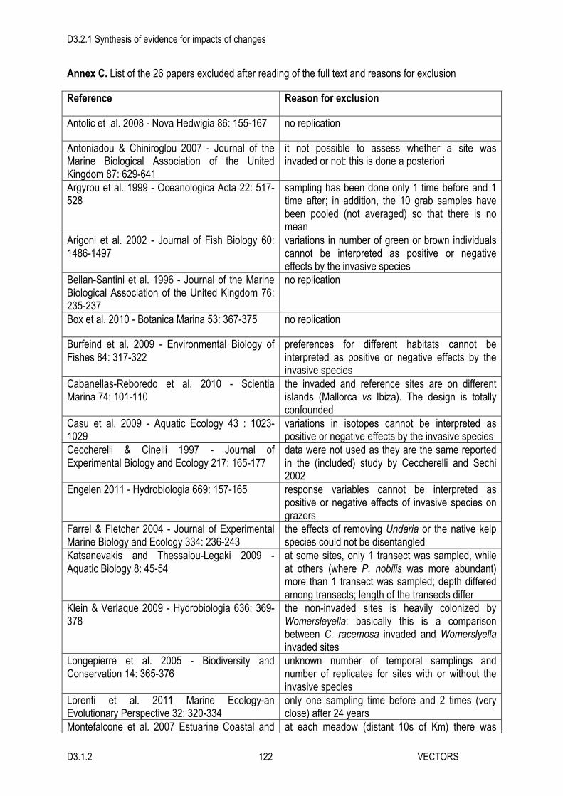
D3.2.1 Synthesis of evidence for impacts of changes  

D3.1.2 122 VECTORS

Annex C. List of the 26 papers excluded after reading of the full text and reasons for exclusion

Reference Reason for exclusion

Antolic et al. 2008 - Nova Hedwigia 86: 155-167 no replication

Antoniadou & Chiniroglou 2007 - Journal of the Marine Biological Association of the United Kingdom 87: 629-641

it not possible to assess whether a site was invaded or not: this is done a posteriori

Argyrou et al. 1999 - Oceanologica Acta 22: 517-528

sampling has been done only 1 time before and 1 time after; in addition, the 10 grab samples have been pooled (not averaged) so that there is no mean

Arigoni et al. 2002 - Journal of Fish Biology 60: 1486-1497

variations in number of green or brown individuals cannot be interpreted as positive or negative effects by the invasive species

Bellan-Santini et al. 1996 - Journal of the Marine Biological Association of the United Kingdom 76: 235-237

no replication

Box et al. 2010 - Botanica Marina 53: 367-375 no replication

Burfeind et al. 2009 - Environmental Biology of Fishes 84: 317-322

preferences for different habitats cannot be interpreted as positive or negative effects by the invasive species

Cabanellas-Reboredo et al. 2010 - Scientia Marina 74: 101-110

the invaded and reference sites are on different islands (Mallorca vs Ibiza). The design is totally confounded

Casu et al. 2009 - Aquatic Ecology 43 : 1023-1029

variations in isotopes cannot be interpreted as positive or negative effects by the invasive species

Ceccherelli & Cinelli 1997 - Journal of Experimental Biology and Ecology 217: 165-177

data were not used as they are the same reported in the (included) study by Ceccherelli and Sechi 2002

Engelen 2011 - Hydrobiologia 669: 157-165 response variables cannot be interpreted as positive or negative effects of invasive species on grazers

Farrel & Fletcher 2004 - Journal of Experimental Marine Biology and Ecology 334: 236-243

the effects of removing Undaria or the native kelp species could not be disentangled

Katsanevakis and Thessalou-Legaki 2009 - Aquatic Biology 8: 45-54

at some sites, only 1 transect was sampled, while at others (where P. nobilis was more abundant) more than 1 transect was sampled; depth differed among transects; length of the transects differ

Klein & Verlaque 2009 - Hydrobiologia 636: 369-378

the non-invaded sites is heavily colonized by Womersleyella: basically this is a comparison between C. racemosa invaded and Womerslyella invaded sites

Longepierre et al. 2005 - Biodiversity and Conservation 14: 365-376

unknown number of temporal samplings and number of replicates for sites with or without the invasive species

Lorenti et al. 2011 Marine Ecology-an Evolutionary Perspective 32: 320-334

only one sampling time before and 2 times (very close) after 24 years

Montefalcone et al. 2007 Estuarine Coastal and at each meadow (distant 10s of Km) there was

D3.2.1 Synthesis of evidence for impacts of changes  

D3.1.2 123 VECTORS

Shelf Science 75: 63-71 only 1 transect at each of 3 depths; values of CI and SI are averages over the three depths for each meadow

Oakes et al. 2011 - Limnology and Oceanography 56: 1824-1831

variations in isotopes cannot be interpreted as positive or negative effects by the invasive species

Pedersen et al. 2005 Aquatic Botany 83: 31-47 no useful data (biomass/cover/growth of the invasive vs those of another alga)

Peirano et al. 2005 Marine Pollution Bulletin 50: 817-822

at each meadow (distant 10s of Km) there was only 1 transect at each of 3 depths; values of CI and SI are averages over the three depths for each meadow

Piazzi & Cinelli 2001 Botanica Marina 44: 509-520 no reference site

Relini et al. 1998 - Biologia Marina Mediterranea 5: 185-195

no replication

Sanchez & Fernandez 2006 - Marine Ecology Progress Series 313: 85-94

no data on the effects of Sargassum on other species

Verlaque & Fritayre 1994 - Oceanologica Acta 17: 659-672

unknown number of replicates

Viejo 1999 - Aquatic Botany 64: 131-149 Sargassum is in pools, while Fucus is not. The comparison between Sargassum and Cystoseira (1 invader versus 1 native) is not useful

Zuljevic 2011 - Biological Invasions 13: 2303-2308

no controls and no replicated sites

D3.2.1 Synthesis of evidence for impacts of changes  

D3.1.2 124 VECTORS

Appendix 3. The diverse effects of marine invasive ecosystem engineers on biodiversity and ecosystem functions Gil Rilov1*, Devin Lyons2, Jonne Kotta3, Henn Ojaveer4, Ana M. Queirós5, Eva Chatzinikolaou6, Christos Arvantidis7, Serina Como8, Paulo Magni9, Andrew Blight10, Helen Orav-Kotta11, Tasman Crowe12, Tamar Guy-Haim13,14 1 Israel Oceanographic and Limnological Research, rilovg@ocean.org.il 2 University College Dublin, devin.lyons@ucd.ie 3 Estonian Marine Institute, University of Tartu, jonne.kotta@sea.ee 4 Estonian Marine Institute, University of Tartu, henn.ojaveer@ut.ee 5 Plymouth Marine Laboratory, anqu@pml.ac.uk 6 Hellenic Centre for Marine Research, evachatz@hcmr.gr 7 Hellenic Centre for Marine Research, arvanitidis@hcmr.gr 8 Consiglio Nazionale delle Ricerche (IAMC-CNR), serena.como@iamc.cnr.it 9 Consiglio Nazionale delle Ricerche (IAMC-CNR), paolo.magni@cnr.it 10 University of St Andrews, ajb34@st-andrews.ac.uk 11 Estonian Marine Institute, University of Tartu, helen.orav@sea.ee 12 University College Dublin, tasman.crowe@ucd.ie 13 Israel Oceanographic and Limnological Research, tamar.guy-haim@ocean.org.il 14 Department of Marine Biology, Charney School of Marine Sciences, University of Haifa, Israel *Corresponding author Keywords: biological invasions; ecosystem engineers; biodiversity; ecosystem functioning ABSTRACT Background: One of the most influential forms of biological invasion is that of invasive ecosystem engineers, species that affect other biota via alterations to the abiotic environment. Such species can have wide-reaching consequences because they alter the physical-chemical structure of ecosystems, changing the rules of existence for broad suites of resident biota. Through these alterations they influence the availability of resources and the impact of stressors that affect other organisms. The objective of this systematic review was to quantify the positive and negative impacts of invasive ecosystem engineers on biodiversity as well as ecosystem functioning, and to identify factors that may cause variation in their impacts. Methods: We have searched two major online databases to conduct a global review and meta-analysis on the impacts of invasive ecosystem engineers on single species and community abundance, and on biodiversity and ecosystem functions in marine and estuarine environments, taking into account a variety of potential effect modifiers (herein, moderators) that included aspects of methodology (laboratory vs. field studies, observational vs. experimental studies) and context (geography, habitat, taxonomy and type of engineer). Results and Discussion: Our analysis revealed highly diverse trends in the overall response of individual species, communities and their function to the presence of invasive ecosystem engineers. Out of the ten effect categories tested, significant negative impacts were found in six, positive effects were observed in two and the last two were neutral, on average. The overall (averaged) effect on individual species was small but negative. At the community level, many studies showed a strong effect of the invader on different community attributes, but the overall summary effect was small and non-significant. In contrast, there was a significant or nearly significant overall strong effect for most ecosystem

D3.2.1 Synthesis of evidence for impacts of changes  

D3.1.2 125 VECTORS

functions considered. Invasive engineers negatively affected growth and metabolic functions, as well as gross primary production (in sediment and water), and they positively affected nutrient flux and decomposition. Effects on sedimentation were variable and overall non-significant but the number of studies found was very low. In the studies included in the analysis, only a very small number simultaneously quantified invaders’ effects on community/diversity and on ecosystem functions in the same system. Such studies could greatly increase our understanding of how invasive species affect functioning through their effects on biodiversity. Most of the subgroup analyses could not explain the observed variability in overall impacts, indicating that moderators other than those considered here may also play a significant role in the determination of the impact of invasive ecosystem engineers. Based on the patterns revealed in this review, we offer a conceptual framework of the different pathways that may lead to impact on ecosystem function and biological communities by invasive engineer plants and epibenthic sessile invertebrates. Ecosystem services are closely linked to ecosystem functions, so the fact that invasive ecosystem engineers strongly affected many ecosystem functions suggests that ecosystem services may also be affected. This subject deserves further study and analysis, and requires the attention of managers and policy makers.

Introduction In modern times, species invasions are amongst the most influential human-derived impacts on Earth’s ecosystems (Primack 1995, Ehrenfeld 2010). Although the terminology is somewhat vague and dependent on use (Pyšek 1995, Ruiz and Carlton 2004), invasive species can be considered a subset of the plethora of alien or non-indigenous species (species that have spread beyond their natural biogeographical range to new regions, usually with human “assistance”) that have already or can potentially induce ecosystem-scale impacts (i.e., significant effects on community biodiversity and/or ecosystem functions), though clear, scientifically-based, demonstrations of ecosystem-wide impacts are actually not that common (Mooney and Hobbs 2000, Simberloff 2011, Sousa et al. 2011, Strayer 2012). This is especially true in the marine environment. Marine biological invasions are a fast-growing environmental concern and are facilitated through the increasing global trade of organisms across oceans, the movement of species within fouling communities and in ballast water, via aquaculture, as live marine seafood and bait, through the aquarium trade and through canals connecting different bodies of water (Rilov and Crooks 2009). Although we have been much slower to realize the extent and impacts of invasions in the sea compared to those on land, the evidence for problematic marine invasions continues to mount (Molnar et al. 2008). For example, the green alga Caulerpa taxifolia, a popular aquarium species, now carpets many square kilometers of seafloor in the Mediterranean suffocating other species; Caulerpa racemosa increases sedimentation and creates an anoxic sediment layer underneath its holdfasts thus causing the degradation of seagrass (Posidonia oceanica) meadows; a comb jelly native to the western Atlantic, was partly blamed for the collapse of fisheries when introduced into the Black and Caspian Seas (Shiganova 1998, Shiganova and Bulgakova 2000); and invasive marsh grasses and mangroves are transforming wetlands around the world (e.g., Neira et al. 2005, Demopoulos and Smith 2010). Invasive ecosystem engineers (abb. IEE), sensu Jones et al. (1994) are potentially one of the most influential forms of bioinvasions on biodiversity and ecosystem functions. Ecosystem engineers (also termed habitat modifiers or bioconstructors) are organisms that exert important control over resource availability for other biota via modulation of the physical and chemical state of the environment. Such species create, destroy, and otherwise modify habitats, and thereby affect both the resources and the organisms that rely on them as well as the abiotic stressors they experience. When they are invasive they also have the potential to have a significant impact on receiving ecosystems (Crooks 2002, Hastings et al. 2007, Crooks 2009).

D3.2.1 Synthesis of evidence for impacts of changes  

D3.1.2 126 VECTORS

Jones et al (1994) distinguished between two types of ecosystem engineers (based on the way they alter the ecosystem. These two types are not mutually exclusive (i.e., a species can be both types). Autogenic engineers modify the environment with their own bodies, which act as part of the engineered habitat and this engineering can be dynamic (when engineers grow they can modify the environment in different ways). For example, as mussels grow, their shells increase the available habitat for other organisms (e.g., by providing settlement space and/or ameliorating environmental stress such as desiccation). Allogenic engineers are species that modify the environment by mechanically changing living and non-living materials (or structures or landscapes) from one physical state to another. Different types and numbers of other organisms will thrive in the area where an ecosystem engineer modified the environment than would have in a non-modified area. The classical examples for such engineers are beavers that alter the flow of rivers by building dams. Mussels can also be considered allogenic engineers. By extensively filtering the water in a lake or a bay they can clear it enough to increase light penetration thus affecting benthic macroalgal communities by facilitating growth. Despite much emphasis on ecosystem engineering in the invasion literature, much of the research has actually only quantified biotic changes, rather than direct effects on ecosystem processes or functions. This is particularly true for terrestrial engineers, whereas, the effects of invasive engineers on ecosystem functioning in aquatic habitats is better documented (Ehrenfeld 2010). We are, however, unaware of comprehensive attempts to investigate and synthesize quantitatively the ecosystem impacts of invasive engineers in either terrestrial or aquatic/marine systems. Several studies and qualitative reviews that explicitly consider marine invaders as habitat modifiers or ecosystem engineers exist (Hastings et al. 2007, Crooks 2009, Jones et al. 2010). Two analyses, one focused on invasive carp and crayfish and another on dreissenid mussels, have examined ecosystem impacts on freshwater systems (Matsuzaki et al. 2009, Higgins and Vander Zanden 2010). However, a comprehensive systematic review of invasive ecosystem engineer impacts that includes meta-analysis on the size and direction of the impacts had yet to be conducted. By providing or modifying habitat, invasive engineers may facilitate the presence of native species with positive effects on abundance and possibly diversity, but they may equally negatively exacerbate abiotic conditions with potentially negative effects on these parameters. As such, understanding the overall effects of invasive ecosystem engineers and mechanisms that may cause variation in their impacts is an important challenge. The purpose of this systematic review was to investigate the current state of knowledge about invasive ecosystem engineers and to provide a meta-analysis that synthesizes impacts on marine ecosystems, including also brackish and transitional waters (i.e. estuaries). We aimed to identify the type, direction and strength of effects of invasive species that are recognized as potential ecosystem engineers. Specifically, we investigated their effects on the abundance of individual native species, community-level abundance (biomass, density, cover) and biodiversity, and on ecosystem functions in the marine environment. The ecosystem functions considered include different measures of primary productivity, sedimentation (related to biotic activity), decomposition rates, nutrient cycling and several proxies for metabolic rates. As the effect of invasive engineers can be context-dependent (even in the same system for the same invader but at different habitats, e.g., Queirós et al. 2011), we investigated the context-dependency of observed effects on several a-priori determined moderators (ecological and methodological) that were perceived to potentially play important roles. Although this is a European project, because of a general lack of such review and synthesis in the literature, we have decided to conduct a global review that includes all regions and all species, using studies that were considered relevant based on specific inclusion criteria described below. Our primary questions were: (1) how strong and diverse (positive vs. negative) is the effect of invasive ecosystem engineers on (a) the abundance of local species, (b) the local biodiversity, and (c) different ecosystem functions?; and (2) are there general patterns in the response of an ecosystem to invasive engineers (and if not, can we identify important modifiers)?

D3.2.1 Synthesis of evidence for impacts of changes  

D3.1.2 127 VECTORS

Methods This study was initiated via a rigorous protocol for the systematic review of literature that adopted a structured Systematic Review procedure suggested by the Collaboration for Environmental Evidence (CEE, http://www.environmentalevidence.org/). This protocol has been published (Rilov et al. 2012). The final review was conducted during 2012-2013, with very small necessary adaptations from the published protocol. Data Collection and Eligibility Criteria A literature search was performed on 18 March 2012 on the Web of Science and Scopus online databases. We used three sets of search terms to capture all considered aspects of the review questions we considered, i.e. the relevant invasive species, the relevant habitats and the relevant effect. These are referred to as the relevant “exposure”, “population” and “outcome”, respectively. The exposure set was designed to identify studies examining invasive species that could potentially be classified as ecosystem engineers; the population set included search terms describing marine and estuarine ecosystems; and the outcome set included general terms for ecosystem structure and functioning. The exact terms for each set were combined using the logical operator 'OR' and the three sets were then combined using the logical operator 'AND' (Annex A). The eligibility of the studies obtained by this search to be included in the final analysis was assessed via an agreed set of inclusion criteria at three levels: title, abstract and full-text. Eligible studies had to include an exposure effect (a potential engineering effect by an invasive species), examine a relevant population (marine or estuarine ecosystem), include a relevant comparison (an experimental or observational comparison between areas or time points with and without invasive ecosystem engineers), and report on a relevant outcome (a measure of ecosystem structure or functioning as defined here). Studies that contained only non-empirical data (e.g., theoretical and modelling studies) were excluded. References were deemed irrelevant and excluded at title level if they dealt with completely unrelated topics. Following this initial screening, we evaluated abstracts of the remaining references according to the inclusion criteria. Finally, we assessed the full text of the references that had been retained. If, at any level, it was unclear whether or not a study met the set criteria, the study was retained for assessment at the next level. To evaluate the degree of agreement on the eligibility criteria, all participants in the analysis (n=11) reviewed an identical subset of the list of references (n=60). The inclusion and exclusion of the subsampled references was tested using Fleiss' Kappa inter-rater agreement test (R Core Team 2012, package 'irr'). The degree of agreement between all participants was found to be satisfactory (kappa=0.56, p <0.001). Disagreements between authors were resolved by discussion and further clarification of criteria against particular studies. We used additional eligibility criteria at the full text level. First, the reported effect had to meet the 'ecosystem engineering' definition (Hastings et al. 2007), i.e. include abiotic and biotic modification components. Given the limited number of studies quantitatively reporting both biotic and abiotic effects, we decided to retain studies that quantitatively reported a biotic effect while the abiotic effect (e.g. reduction in light) could be described only qualitatively. Secondly, after screening the results for outcomes with sufficient replication to enable a meta-analysis, we focused on studies that reported the following outcomes: 1) single species abundance; 2) community abundance; 3) species richness; 4) species diversity (Shannon index); 5) community evenness (Pielou index); 6) gross primary productivity; 7) sedimentation; 8) decomposition; 9) growth and metabolic functions; 10) nutrient cycling. Thirdly, we excluded studies that failed to provide the set of parameters required for the calculation of the effect size (Hedges’ g): means, sample sizes and variance estimate (standard deviation or standard error) with and without the invasive ecosystem engineer.

D3.2.1 Synthesis of evidence for impacts of changes  

D3.1.2 128 VECTORS

The screening process resulted in a final set of references some of which contained data for multiple outcomes. In such cases, each outcome was considered to be an independent dataset, and is henceforth referred to as a 'study'. Data Extraction and Effect Size Calculation Means, sample sizes and variance estimators were extracted directly from the text and tables, or from figures using the image analysis software ImageJ (Schneider et al. 2012) and DataThief III (Tummers 2006). For multi-factorial designs, factor information was recorded. Potential moderators, i.e., factors that may modify the effect of the analysed invasive ecosystem engineer species were recorded for each study and considered in subsequent analyses We used Hedges' g as the effect size. Hedges’ g is the unbiased mean difference in the response variable between the ‘treatment’ (invasive ecosystem species present) and control (invasive ecosystem species absent) groups, standardized by the within-group standard deviation. It transforms all effect sizes to a common metric, thus enabling the calculation of summary effects using data in different scales (Borenstein et al. 2011).

Hedegs' g (Hedges 1981) is defined as:

(1) – 1–

where is the mean of the response variable in the invasive ecosystem engineer treatment, is the mean in the control, is the within-groups standard deviation pooled across groups, and df are the degrees of freedom used to estimate according to the formula:

(2)

where niee and nc are sample sizes, Siee and Sc are standard deviations of the invasive ecosystem engineer treatment and control, respectively. The variance of g was calculated as:

(3) 1–

–

In case of matched (paired) groups or pre-post design (e.g., BACI), the intra-class correlation coefficient (ICC), was used to calculate an adjusted effect size variance (Borenstein et al. 2011). When the full text did not provide sufficient information to calculate ICC, it was assumed to be 0.5, thus allowing for a narrower variance within study than in non-correlated studies (ICC=0.0), and wider than highly correlated ones (ICC→1.0). Studies often reported data on more than one time-period (a time-series data), for the same sampled population (i.e. repeated measurements designs). In such scenarios, we distinguished between two cases. When the time-series of the measured effect was accompanied with a congruent time-series of the predictor (invasive ecosystem engineer species abundance), we selected two time-points for analysis: the time-point of the maximal IEE abundance was regarded as the treatment group, whereas the latest time-point of minimum observed abundance (or absence) was regarded as the control group. Over time, the effect of an invasive species may fluctuate, depending on various environmental factors (Harlin and Villalard-Bohnsack 2001) and food-web interactions (Nyström et al. 2001). When such time series were documented in a study, neither the end-point of a time-series nor the sum of measurements over time may reflect the true effect of the invasive species on the ecosystem. For this reason, when available, we chose the measurements corresponding to minimal and maximal invasive abundances. When there was no information regarding the effector's abundance, we summed the effect size by applying fixed-effect model analysis (Borenstein et al. 2011). Similarly, dependent subgroups within a study, such as different measures for the same outcome or multiple levels within treatment and control groups, were summed using the fixed-effect model. In cases where publications contained information

D3.2.1 Synthesis of evidence for impacts of changes  

D3.1.2 129 VECTORS

on multiple independent experiments or experiments that were conducted at sites separated by >1 km (which we consider independent enough), we computed separate effect sizes for each experiment. Meta-Analysis The effect size estimates from individual studies were aggregated using the software Comprehensive Meta-Analysis v.2.2.064 (Borenstein et al. 2005). Typically, studies included in the same outcome category had different designs, target populations, measurement protocols, and other experimental characteristics. Thus, the outcomes were considered heterogeneous. In this case, the adequate summary effect model structure is a random-effects model. Random-effects meta-analysis estimates the mean from a distribution of effects rather than a common true effect size, as assumed in the fixed-effect model (Borenstein et al. 2011). We interpreted asymmetrical funnel plots as an indication of publication bias, as these display the relationship between the effect size and standard error. The Trim and Fill algorithm (Duval and Tweedie 2000) was also used to evaluate publication bias. This is a non-parametric iterative procedure that provides an adjusted estimate of effect size that includes the expected value of missing studies that would create a symmetrical funnel plot. This provides an estimate of what the effect size would be if the dataset were unaffected by publication bias. The imputed studies and the unbiased effect sizes were computed and displayed on the funnel plots together with the observed studies. Moderator Analyses Study-level covariates may contribute to effect size variation and can thus be regarded as potential effect moderators. These covariates can be related to either the characteristics of the studied species/habitats/regions or the study itself (i.e. methodology used). For each outcome category we defined six “characteristic” moderators: engineering type, study type, study settings, the taxonomical attribution of the invasive ecosystem engineer, habitat and geographic region. Every moderator divided the outcome studies into subgroups. Engineering type included three subgroups: autogenic, allogenic, and a third subgroup of species or effects that can be considered as both autogenic and allogenic. In this category, we assigned the engineering type according to the type of effect that was measured, suggested or discussed in the specific paper from which each study was drawn. Autogenic effects are easier to describe and interpret, whereas allogenic effects are more difficult to determine; thus allogenic effects were often not measured directly, but inferred from the full text of the reference. We used two methodological moderators: study type, i.e. observational vs. experimental studies (where manipulative procedures associated with the IEE were carried out); and the study setting, i.e. field vs. laboratory studies. Study region was defined according to the geographic coordinates provided in the assessed texts, and aggregated into biogeographic categories based on the large marine ecosystems defined by Sherman & Hempel (2009). To assess the relationship between the potential effect moderators and the effect size within each outcome category, we performed subgroup analyses using a mixed effects model structure. This model applies a random-effects model within subgroups and a fixed-effect model across subgroups to compute the overall effect (or “summary effect”), allowing for tests of heterogeneity as well as for tests of random effects models once the variability accounted for by moderator variables has been removed (Lipsey and Wilson 2001). In testing overall (summary) effects, we relaxed the significance level in acknowledgement of the diversity of data used, and considered statistical probabilities of p≤0.07 associated with the null hypotheses as significant if n>10 studies and the 95% confidence intervals do not or barely cross the 0 line of Hedges’ g. For individual studies and subgroups we consider the traditional α<0.05 for statistical significance.

D3.2.1 Synthesis of evidence for impacts of changes  

D3.1.2 130 VECTORS

Results Our search yielded 2587 references. Of these, 1276 were excluded at title level screening, with a further 1065 excluded at abstract level. Of the 246 references retained, 165 were excluded after full-text assessment: if only non-engineering effects were measured (n=3); if insufficient information to determine an engineering effect was provided (n=65); if an irrelevant outcome was measured (n=48); if no appropriate intervention or control group was described (n=18); if non-marine or estuarine habitats were assessed (n=5); if only theoretical or non-quantitative data (n=22) were given; and if no adequate data for effect size calculation were actually provided (n=4). From the remaining 81 references, we extracted 257 studies that allowed for the calculation of effect sizes. All but 6 of the included papers were published after the year 2000. Study and data characteristics The majority of the included references (56%) did not use the term "ecosystem engineer" or its synonyms, e.g. "foundation species", "bio-constructors" and "habitat modifiers", to describe the effect type of the invasive species. Instead, in those references, ecosystem engineering effects were inferred from the study context. Fifty seven percent of the studies were observational, i.e., describing an effect rather than forming it by manipulation (Fig. 1). These included before-after designs and comparisons between multiple sites. The vast majority of the studies (97%) were conducted in the field (Fig. 1), and the rest in the lab. Fifty seven percent of the studies described an autogenic effect, 31% described an allogenic effect, and the remaining 12% described combined effects (Fig. 2). For example, Cottet et al. (2007) found that the invasive cordgrass Spartina anglica alters mudflat community, both by direct increase of habitat heterogeneity via the physical presence of the grass structure (autogenic effect), and by increases in sediment accumulation and modification of hydrographic features (allogenic effect). Sixty-eight percent of the invasive ecosystem engineer species in the studies we analysed were plants (Fig. 3), including seaweeds (algae), grasses (this category includes seagrasses and saltmarsh plants) and mangroves. Of the rest, the most prominent groups were bivalves (15%) and worms (8%). The most studied species were the seaweeds Caulerpa taxifolia and C. racemosa. In 17% of the included studies (44 out of 257), one or more of the local species affected by the IEE are known to be, or are described in the paper as being under the threat of global or local extinction (i.e. considered ‘vulnerable’ or ‘endangered’ according to the IUCN Red List). For example, seven different publications (Brusati and Grosholz 2006, Hammond and Griffiths 2006, Brusati and Grosholz 2007, Chen et al. 2007, Gan et al. 2009, Zhou et al. 2009, Holsman et al. 2010) describe the effects of the vigor hybrid cordgrass (Spartina alterniflora X S. foliosa) on the local biota, including the threatened local Spartina cordgrass. The study regions included the coasts and estuaries of all continents except Antarctica (Fig. 5), with an apparent bias towards the California Current and the Gulf of California (17%), followed by the Mediterranean Sea (15%), the Celtic-Biscay Shelf (8%), the Insular Pacific-Hawaiian (8%), the North Sea (7%), and the Baltic Sea (2%). The three regional seas considered in VECTORS accounted for 24% of the studies. Highly studied habitats (Fig. 4) include sandflats (22%), the rocky intertidal (16%), mudflats, lagoons and estuaries (10-12% each). The outcomes with the highest number of studies were abundance categories (community abundance, 21%; single species abundance, 18%; species richness, 16%), whereas the studies related to ecosystem functions were less numerous (2-7% each, except nutrient fluxes - 14%, Fig. 6). Of the 81 papers, only nine reported effects on both community structure and some ecosystem functions, and eight reported effects on single species and ecosystem function (Annex B). Of these, very few papers

D3.2.1 Synthesis of evidence for impacts of changes  

D3.1.2 131 VECTORS

reported results on the same or similar ecosystem functions, limiting our ability to directly assess the relationship between community or single species responses, and ecosystem functions. Overall and subgroup analyses of the 10 outcome categories, and of the corresponding publication bias in each, are detailed below. Overall outcome patterns Out of the 10 outcome categories, overall significance was identified for the effect on single species abundance among the abundance/diversity categories. In contrast, four out of the five ecosystem functions overall effects were significant and strong. Regardless of significance, six of the 10 categories had a negative sign and two were positive and two were near neutral (Fig. 6). Single-Species Abundance We found 46 relevant studies examining the effects of IEE on single-species, including 25 observational and 21 experimental studies, from 37 different publications (Fig. 7). Twenty-seven studies examined autogenic engineers; 13 examined allogenic effects; and six studies described simultaneous allogenic and autogenic effects. The studied regions spanned 15 large marine ecosystems, with the majority originating in the Mediterranean (n=7). Twenty nine of the studies focused on the effects of plants: Spartina (n=3), Lophocladia (n=2), Gracilaria (n=1), Caulerpa (n=12), Phragmites (n=3), Sargassum (n=3), Codium (n=4), and Undaria (n=1). Others focused on the effects of the bivalves Crassostrea (n=3), Mytilus (n=1), Musculista (n=2), and Potamocorbula (n=1); the gastropod Batillaria (n=1); the annelids Ficopomatus (n=3), Sabella (n=3), and Marenzelleria (n=2); and the crabs Carcinus (n=1) and Petrolisthes (n=1). Although 32 of the 46 individual effect sizes were statistically significant (of the 32, 17 were negative and 15 positive), the overall effect size of the presence of invasive ecosystem engineers on single species abundance was relatively small but ecologically significant (Hedges’ g ± 95% C.I. = -0.2012 ± 0.203, p=0.052, Fig. 7). Of the different taxonomic subgroups, the only one that presented a significant effect were the seaweeds Rhodophyta (p<0.001) and Chlorophyta (p=0.049), both of which had negative effects - (Fig. 8D). From the reviewed habitat types, coral reefs (p=0.012) and harbours (p=0.024) were those in which IEE had statistically significant summary effects within the subgroup. IEE had positive effects in single species abundances in coral reefs, but negative effects in harbours (Fig. 8E). Of the 15 studied regions, IEE had significant effects only in three: in the Baltic Sea (p=0.001), and the Celtic-Biscay Shelf (p=0.048) summary effects were positive; and in the Iberian Coastal region (p=0.019) the effects were negative (Fig. 8F). Lab studies (n=5) were strongly negative and statistically significant (p=0.01), whereas field studies (n=41) were mildly negative and non-significant. No differences were found between study types and engineering types in their overall effects, and none of the individual subgroup effects were statistically significant (Fig. 8). Community Abundance We found 55 relevant studies examining the community abundance effects of invasive ecosystem engineers, including 33 observational and 22 experimental studies from 41 different publications (Fig. 9). All studies were performed in the field. Forty studies tested autogenic engineering effects; 11 tested allogenic effects and four studies described a combined effect. The majority of studies originated in the California Gulf and Current (n=12). Of the rest, seven were from the North and Baltic seas, and seven from the Mediterranean Sea. Thirty-four of the studies focused on the effects of plants: Spartina (n=10), Rhizophora (n=4), Sargassum (n=7), Gracilaria (n=1), Caulerpa (n=7), Phragmites (n=1), Codium (n=3), and Fucus (n=1). Others focused on the effects of the tunicates Bothrylloides and Didendum (n=1), the bryozoan Watersipora (n=3), the bivalves Mytilus (n=3), Musculista (n=2), Dreisenna (n=2), Crassostrea (n=3), Pinctada (n=1), the worms Ficopomatus enigmaticus (n=2) and Sabella spallanzanii (n=3), and the crab Petrolisthes (n=1).

D3.2.1 Synthesis of evidence for impacts of changes  

D3.1.2 132 VECTORS

Testing the effect of invasive ecosystem engineers on community abundance showed that 27 of 55 individual effect sizes were statistically significant (some with very strong effects); of them, 14 were negative and 13 positive, and the overall effect size was very small and non-significant (Hedges’ g ± 95% C.I. = 0.03 ± 0.172, p=0.761, Fig. 9). Of the engineering types, allogenic and autogenic engineering had positive but non-significant effects and the combined engineering type had a significant negative effect (Fig, 10C). The only taxonomic group causing significant effects was Chlorophyta, which had a negative overall effect (Fig. 10B). Of all habitat types, only coral reefs were significantly (negatively) affected (Fig. 10E). In the Gulf of California, there was a positive significant effect (Fig. 10D). Experimental studies revealed a positive overall effect whereas observational studies revealed negative effects, but none of these effects were statistically significant (Fig. 10A).

Species Richness We found 42 relevant studies examining the effects of IEE on species richness, including 30 observational and 12 experimental studies, from 28 different publications (Fig. 11). Twenty five studies quantified effects of autogenic engineers; ten quantified effects of allogenic engineers and seven studies described a combined effect. Most studies came from the Pacific coast (n=9), eight from the western Atlantic, six from the Celtic-Biscay shelf, five from the Mediterranean Sea, four from the North Sea, three from Australia, and one each from the East China Sea and the Benguela current. 32 of the studies focused on the effects of plants: Spartina (n=4), Rhizophora (n=2), Sargassum (n=2), Caulerpa (n=2), and Undaria (n=1). Others focused on the effects of the tunicates Bothrylloides and Didendum, the bivalves Mytilus (n=3), Musculista (n=2), Crassostrea (n=1) and Pinctada (n=1), and the crab Petrolisthes (n=1). Half (21) of the studies assessing effects of IEE on species richness led to significant effect sizes, 9 negative and 12 positive; the overall test was positive but non-significant (Hedges’ g ± 95% C.I. = 0.059 ± 0.290, p=0.609, Fig. 11). This heterogeneity could not be explained by study type, study setting or engineering type in the subgroup analysis (Fig. 12). Of the taxonomic groups assessed, only Bivalvia had a significant (positive) effect (Fig. 12D). Non-significant effect sizes were estimated for all habitat subgroups, with the exception of oyster beds (Fig 12E), where significant negative effect sizes were observed. Significant effect sizes were observed for studies done in the Celtic-Biscay Shelf and the Gulf of California (positive effects) and in the Mediterranean (negative effect, Fig. 12F). Species Diversity We found 18 relevant studies examining the effects of invasive ecosystem engineers on species diversity, using the Shannon Index (H') as a measure. These included 12 observational and six experimental studies from 11 different publications (Fig. 13). Nine studies examined autogenic engineers; six examined allogenic effects and three studies described a combined effect. Five studies came from the California current, two from Insular-Pacific, three from the Scotian shelf, two from the Celtic-Biscay shelf, three from the Mediterranean Sea, and one from each of the following: Patagonian shelf, East China Sea and the Benguela current. Eleven of the studies focused on the effects of plants: Spartina (n=4), Rhizophora (n=2), Sargassum (n=2), Caulerpa (n=2), and Undaria (n=1). Others focused on the effects of the bivalves Mytilus (n=5) and Pinctada (n=1), and the bryozoan Watersipora (n=1). As with species richness, although 8 of 18 individual effect sizes were statistically significant (5 negative and 3 positive), we found that invasive ecosystem engineers had very little to no overall effect on species diversity (Hedges’ g ± 95% C.I. = -0.148 ± 0.450, p=0.517, Fig. 13). This heterogeneity could not be explained by the subgroup analyses. No differences were found between taxonomic groups, engineering types, habitats and study types in their overall effects, and none of the individual subgroup effects were statistically significant (Fig. 14). Of the eight study regions, an overall significant effect was found only for the Mediterranean, where impacts were strongly negative (Fig. 14E).

D3.2.1 Synthesis of evidence for impacts of changes  

D3.1.2 133 VECTORS

Community Evenness We found 12 relevant studies that tested effects on community evenness, including three experiments and nine observational studies from 6 different publications (Fig. 15). Four studies tested autogenic engineers; five tested allogenic effects and three studies described a combined effect. Most of the invasive engineering species are plants: Rhizophora (n=2), Spartina (n=3), Caulerpa (n=1) and Sargassum (n=2). Other species are bivalves: Pinctada (n=1) and Mytilus (n=3).The majority of the studies have been conducted in the Pacific, with five from the California Current, two from the Insular-Pacific, three from the Scotian Shelf, two from the Mediterranean, and one from the Celtic-Biscay shelf. Most of the studies are from soft bottom habitats: sandflats (n=2), mudflat (n=1), and lagoons (n=6). The remaining studies were conducted in mangrove forests (n=2) and the rocky intertidal (n=1). In the case of effects on evenness, only 3 of the 12 individual effects were significant and the overall effect was non-significant (Hedges’ g ± 95% C.I. = -0.411 ± 0.477, p=0.091, Figure 15). The subgroup analyses for the effects of engineering type on community evenness showed that autogenic effects were significantly positive, while the allogenic and combined effects were negative and non-significant (Fig. 16C). As observed in the species diversity category (Fig. 14), the one region with a significant effect was the Mediterranean, again strongly negative (Fig. 16E). No differences were found between different taxonomic groups, habitats or study types in their overall effects, and none of the corresponding individual subgroup effects were statistically significant (Fig. 16). Gross Primary Productivity We found 12 relevant studies examining the gross primary productivity effects of invasive ecosystem engineers, including three observational and nine experimental studies from nine different publications (Fig. 17). All but one of the studies estimated benthic productivity using Chlorophyll a measurements in the water column (n=4) or in sediment (n=7). One study used δ^13C isotopic signal as a productivity measure. Four studies examined autogenic engineers; six examined allogenic effects and two studies described a combined effect. Four studies came from the California current, two from Patagonian shelf, three from the Iberian Coast, one from the Mediterranean, one from the Caspian Sea, and one from the North Sea. Seven of the studies focused on the effects of plants: Spartina (n=3), Sargassum (n=2), Zostera (n=1), and Caulerpa (n=1). Others focused on the effects of the worms Ficopomatus (n=2) and Marenzelleria (n=1), the gastropod Batillaria (n=1), and the comb jelly Mnemiopsis (n=1). In general, the presence of invasive ecosystem engineers caused a significant decrease in gross primary productivity (Hedges’ g ± 95% C.I. = -0.483 ± 0.517, p=0.067). Eight of 12 individual effect sizes were statistically significant; six of these were negative (Fig. 17). In the moderator analyses (Fig. 18) three had shown significant differences among subgroups. Engineering type encompassed both allogenic and autogenic effects was strongly negative and significant (p<0.001), yet represented a small sample size (n=2). Other significant moderator subgroups included lagoons in the habitat analysis (p=0.02) and Patagonian Shelf in the regional analysis (p=0.02), both presenting negative effects. Sedimentation rate We found five relevant studies examining the effects of invasive ecosystem engineers on sedimentation rate, including three observational and two experimental studies from three different publications (Fig. 19). All studies but one examined autogenic engineering effects. Three studies came from the Mediterranean Sea, one from the California Current, and one from the Gulf of Alaska. All the studies focused on the effects of plants: Spartina (n=2), and Caulerpa (n=3). All the studies were performed in tidal sandflats. The total computed summary effect of invasive ecosystem engineers on sedimentation was not significant (Hedges’ g ± 95% C.I. = -0.447 ± 0.886, p=0.322). Three of five individual effect sizes were

D3.2.1 Synthesis of evidence for impacts of changes  

D3.1.2 134 VECTORS

significant, two were negative and one positive (Fig. 19). No differences were found between regions, taxonomic groups, engineering types and study types in their overall effects, and none of the corresponding individual subgroup effects were statistically significant (Fig. 20). Decomposition We found 13 relevant studies examining the effects of invasive ecosystem engineers on decomposition, including four observational and nine experimental studies from 8 different publications (Fig. 21). Six studies examined autogenic engineers; five examined allogenic effects and two studies described a combined effect. Four studies came from the California Current and the Gulf of California, two from Iberian coastal, three from the Mediterranean Sea, and one each from the Patagonian Shelf, Celtic-Biscay Shelf and the North Sea. Ten of the studies focused on the effects of plants: Spartina (n=4), Sargassum (n=2), Zostera (n=1), and Caulerpa (n=3). Others focused on the effects of the worms Ficopomatus (n=1) and Marenzelleria (n=1), and the bivalve Musculista (n=1). Measurement methods varied between studies: six used organic matter as a proxy for decomposition, four used sulfate reduction, two used carbon content, and one used total mass loss. We found that invasive ecosystem engineers had an overall positive effect on decomposition though it was marginally non-significant (Hedges’ g ± 95% C.I. = 0.486 ± 0.527, p=0.070). Six of 13 individual effect sizes were statistically significant, five were positive and one negative (Fig. 21). Potential effect moderator analyses (engineering type, engineering species taxonomic group, habitat type, study type, study region) failed to show significant differences between different subgroups (Figure 22). Nutrient Flux We found 36 relevant studies examining the effects of invasive ecosystem engineers on nutrient fluxes, including 23 observational and 13 experimental studies from 14 different publications (Fig. 23). Twenty-two studies tested the effects on inorganic nutrients whereas 14 studies tested the effect on organic nutrients. The tested nutrients varied between studies: 13 measured carbonic compounds (e.g., dissolved inorganic carbon, dissolved organic carbon, particulate organic carbon), 13 tested nitrogen compounds (e.g., nitrate, nitrite, ammonium), 4 tested phosphatic compounds, 4 tested sulfuric compounds, and 1 tested silicate. Twenty-four studies examined autogenic effects, 11 examined allogenic effects, and one examined a combined effect. Ten studies came from the Mediterranean Sea, 7 from the Caspian Sea, 6 from the California Current, one from the Celtic-Biscay shelf, one from the North Sea, two from the East China Sea, one from the North east US continental shelf, and 8 from Insular Pacific. 28 of the studies focused on the effects of plants: Caulerpa (n=10), Zostera (n=7), Rhizophora (n=8), Spartina (n=2) and Gracilaria (n=1). The rest focused on the effects of the gastropod Crepidula (n=1) and the comb jelly Mnemiopsis (n=7). Overall, the presence of invasive ecosystem engineers caused a significant positive effect on nutrient fluxes (Hedges’ g ± 95% C.I. = 0.568 ± 0.267, p<0.001). Twenty of 36 individual effects were significant, 4 of these negative and 17 positive (Figure 24). Allogenic engineers had a strong, significant positive effect on nutrient fluxes while the effect of autogenic engineers was smaller and non-significant (Fig. 24B). The effect of IEEs on inorganic nutrients was strong and positive whereas the effect on organic nutrients was smaller and non-significant (Fig. 24E). The effect on the fluxes of carbon, nitrogen and phosphorus was positive and significant (or nearly significant), whereas the effect on silicate was nearly zero, and the effect on sulfur was negative and highly variable; both were non-significant. Observational studies revealed significant positive effects while experimental studies were positive but non-significant (Fig. 24A). Of the five invasive engineer taxonomic groups, three were associated with significant positive effects: Angiosperms (n=17), Ctenophora (n=7) and Gastropoda (n=1), whereas Chlorophyta (n=10) and Rhodophyta (n=1) were associated with non-significant zero or negative effects (Fig. 24A). The (positive) effect of invasive engineers on nutrient flux in open coasts, salt marshes and mangrove forests was greater than in other habitats (Fig. 24D). Of the studied regions (Fig. 24G), positive

D3.2.1 Synthesis of evidence for impacts of changes  

D3.1.2 135 VECTORS

significant effects (p<0.001) were found for the Caspian Sea, Celtic-Biscay Shelf, East China Sea, and Insular Pacific-Hawaiian. Growth and metabolic functions We found 18 relevant studies examining the effects of invasive ecosystem engineers on metabolic functions (e.g., growth rates, feeding rates) of the surrounding biota, including 6 observational and 12 experimental studies from 16 different publications (Fig. 25). Eight studies examined allogenic effects; 8 examined autogenic effects and two studies described a combined effect. Four studies came from the California Current, four from the Celtic-Biscay shelf, three from the North Sea, one from the eastern US continental shelf, two from Insular Pacific, two from the Mediterranean, one from southeast Australia, and one from the Iberian Coast. Ten of the studies focused on the effects of plants: Spartina (n=1), Sargassum (n=2), Codium (n=1), Rhizophora (n=2), and Caulerpa (n=3). Others focused on the effects of the gastropods Crepidula (n=2) and the periwinkle Littorina (n=1), the annelids Sabella (n=1) and Marenzelleria (n=1) the bivalves Crassostrea (n=1), Musculista (n=1) and Potamocorbula (n=1). Measurement methods varied between studies: nine tested growth rate, two measured mean body size, two studied predation rate, two studied calcium carbonate precipitation, two studied carbon uptake, and one studied enzyme activity - all of native species. Although the measurement methods varied, the presence of invasive ecosystem engineers caused an overall significant negative effect on metabolic functions (Hedges’ g ± 95% C.I. = -0.699 ± 0.449, p=0.002). Eleven of 18 individual effects were significant, nine negative and two positive (Fig. 25). Study type analysis revealed that experimental studies had a significant negative effect on community metabolic functions while the effect in observational studies was smaller and non- significant (Fig. 26A). The overall effect reported from field studies was significantly negative, whereas effects studied in the lab were non-significant overall (Fig. 26B). Both autogenic and allogenic effects were significantly negative and very similar, while combined autogenic-allogenic engineers had a non-significant effect overall (Fig. 26C). Habitat analysis revealed a greater effect of invasive engineers in rocky intertidal and estuarine habitats (Fig. 26E). The only significant effect in a regional analysis was a negative effect in the North-East U.S. continental shelf (Fig. 26F).

Publication Bias The funnel plots for the relationship between the moderator subgroups effect size and standard error were not asymmetrical (Fig. 27). Furthermore, the adjusted effect sizes, calculated using the trim-and-fill method, were not substantially different from the initial estimates suggesting the absence of significant publication bias. Discussion This systematic review and meta-analysis offers the first quantitative global synthesis of the effects of invasive ecosystem engineers on both biodiversity and ecosystem functions. To the best of our knowledge, no such analysis currently exists either in terrestrial or aquatic systems. The understanding of the impact of invasive ecosystem engineers on communities and functions in marine systems has greatly improved in the past two decades, since the term “ecosystem engineers” was suggested by Jones et al. (1994). We found studies from a large variety of species, habitats and regions around the globe, making this analysis broad and robust. Biogeographic and habitat biases were present, however, with a striking majority of studies focusing on plant IEEs and outcomes. This bias is perhaps natural, as plants are conspicuous engineers and successful invaders, making them a relatively accessible study object. Nevertheless, some caution should be taken in the generalization of our findings. One striking aspect of the studies we assessed was the low number of those that investigated IEE impacts on community/diversity and ecosystem functions simultaneously in the same system, a gap that should be quickly recognized by the research community. In the past two decades, research on the

D3.2.1 Synthesis of evidence for impacts of changes  

D3.1.2 136 VECTORS

relationship between biodiversity and ecosystem functions (BEF) has been at the forefront of ecology, with heated debate around theory, models and empirical evidence linking the two (Schwartz et al. 2000, Loreau et al. 2001, Hahn 2003, Hooper et al. 2005, Zavaleta et al. 2010, Connolly et al. 2013, Mouillot et al. 2013, Pasari et al. 2013). Improved understanding of this relationship has become an urgent need due to the magnitude and speed of human-induced changes to the environment through direct impacts on biota. The need to understand the consequences of that change is critical for management given the close linkage between species, ecosystem functions and services (Kremen 2005, Gamfeldt et al. 2013). This is especially true in the context of bioinvasions, and even more particularly so for invasive engineers that have the potential for very high impacts on both diversity and function. In the past decade, understanding the importance of the link between biodiversity and ecosystem functions, and their importance to ecosystem resilience and stability has been emerging - although the mechanisms are still poorly understood in many cases (Hooper et al. 2005, Loreau and Mazancourt 2013). In light of this, we encourage future studies to test the effects of IEE on diversity and functions (and preferably several relevant functions) in the same investigation, and aim to further disentangle possible mechanisms of impact. Because of the clear link between species attributes (traits) and functions (Wood et al. 2010, Drenovsky et al. 2012, Lindo et al. 2012, Paganelli et al. 2012), we also call for the inclusion of species traits analysis in this type of study. Our analysis revealed highly diverse trends in the response of individual species, communities and their function to the presence of invasive ecosystem engineers. At the individual species level, the overall effect was small and negative. Interestingly however, no significant overall effect was found in any of the categories where community level effects were assessed, while for most ecosystem functions there was a significant or nearly significant overall effect. This is especially surprising given the fact that significantly fewer studies focusing on function were reviewed and that different functional parameters were then necessarily aggregated for analysis within each category (e.g. all nutrients were aggregated under organic and inorganic cycling). If we examine only the direction of the summary effect sizes (regardless of significance, Fig 6), negative impacts were found in the majority of categories related to recipient ecosystems. It is important to note that a near-zero overall effect on community parameters may not be a true representation of the real effects of invasive engineers; but rather points to the complex nature of the interactions between the IEE and the different components of the invaded community. Within a community, some species may be facilitated by the IEE while others may be suppressed, either directly by the invader, or indirectly by direct competition or predation by species facilitated by the IEE (e.g. trophic cascades). Overall, these effects may cancel each other out when measured at the community level. Hence, quantifying effects on components of diversity changing between impacted and non-impacted communities (e.g. β diversity, Whittaker 1972, Anderson et al. 2011) may help to elucidate pathways of impact for IEE. It is extremely challenging to decipher and disentangle such complex interactions, especially in field observations and experiments. These diverse and sometimes contrasting responses of different native species to the presence of an invasive engineer could be seen in the few examples where studies reported on effects on multiple species, which were aggregated to estimate community responses in our analysis. This is nicely exemplified in Neira et al (2007), one of the studies included in our meta-analysis, where varied effect sizes were observed in response to the invasive Spartina across single species and taxonomic groups. In the same study, the importance of the context of comparison between invaded and un-invaded areas also stands out, highlighting how comparing a mature invasion to pre and post invasion areas can result in very different outcomes. The very detailed data published in that study were used to estimate effect size calculations for each of the listed species. In Fig. 28 we refer to four different experimental manipulations described by the authors, comparing pairs of the following zones: invaded plot versus an

D3.2.1 Synthesis of evidence for impacts of changes  

D3.1.2 137 VECTORS

adjacent post-invasion (dieback) plot (experiment 1), mature plot versus a plot on which all Spartina canopy was clipped and removed (experiment 2), mature plot versus un-invaded plot (experiment 3a), and an invaded plot with progressed Spartina community (mature) versus a dieback plot (experiment 3b). In this analysis, it is easily seen that different local taxa within the same experiment showed effect sizes of different strength and direction. For example, the effect of a mature invasion on the abundance of the oligochaete Tectidrilus diversus is significantly positive, while the polychaete Fabricia sp. is significantly negatively-affected. Secondly, we see that the different experimental comparisons, using different invasion stages to represent the treatment groups and three different conditions (un-invaded, clipped and dieback plots) as control groups, yielded different and even opposite overall effect sizes. Comparisons of mature plots versus un-invaded plots had a significant overall negative effect, while comparing mature plots to clipped or dieback plots (i.e., post invasion plots) had significant overall positive effects. Neira et al (2007) suggested that the Spartina invasion caused a community shift from microalgae feeders to below ground detritus consumers, followed by anaerobic and toxic conditions leading to mass mortality of Spartina and its associated biota. This case study demonstrates that when one compares a community or a function between plots with and without an invader, it is important to know if a “without” plot or area is one where the invader was never present, it was present but naturally (recently) disappeared or was experimentally removed. The outcome can be very different if the invader can leave its environmental and ecological footprint in the system even after it is physically not there, at least for some ecologically meaningful period (months, years). Our findings support the long-term perspective suggested by Strayer et al. (2006) whereby the influence of an invasive species on the ecosystem includes both acute and chronic effects, varies over time and may be long-lasting. It also reinforces the perspective taken here that invasion phases should be considered when comparing experiments. Opposing effect sizes (negative and positive) in individual studies, both in species and community level outcomes, are not surprising, as the strength and direction of the effect are also presumably highly context-dependent (e.g. the identity of the invasive species, its taxonomic group, the invaded ecosystem as well as many other moderators). The subgroup analyses carried out here were aimed to test if some well-defined categories were likely to influence the strength and direction of the effects that could explain this diversity in responses. However, many sub-groups considered here included a small number of studies, which may have hindered our ability to discriminate those different effects adequately. We focused here on those for which sufficient data for analysis was found. Within most taxonomic groups of invasive engineers, effect sizes varied greatly (i.e. had large confidence intervals) and in many cases had low n (reducing the power of analysis) such that a significant effect could not be detected. Exceptions are Rhodophyta that had clear negative effects on single species abundance; Chlorophyta, which had negative effects on single species and community abundance; and Bivalvia, which were found here to have positive effects on species richness. The negative effects of the seaweeds are, in most cases, caused by smothering or reducing irradiance to the native flora. For example, the Rhodophyta Lophocladia lallemandii is an epiphyte on the seagrass Posidonia oceanica and it was suggested that by reducing light it reduces growth of the native seagrass (Drouin et al. 2011). However, it can also affect negatively the biota associated with the seagrass (bryozoans), possibly by reducing settlement surface area and changing the flow regime that could reduce food supply to the epiphytic bryozoan. In the case of the red algae Gracilaria vermiculophylla, its impacts on the seagrass Zostera marina were only detected in combination with increased temperature (Dijkstra and Harris 2009), indicating the context-dependency of the effect itself (Deudero et al. 2011). The invasion of the green algae Caulerpa scalpelliformis on deep reefs of Botany Bay in Australia reduced the cover of many encrusting invertebrate groups including sponges, colonial ascidians and bryozoans, and this reduction was suggested to be due mainly to the sediment trapped by the stolons of the alga (Ferrer et al. 1997), an allogenic effect that may strongly affect these filter feeders. The invasion of the chlorophyte C. racemosa was suggested to impact community abundance through a decline in the density of

D3.2.1 Synthesis of evidence for impacts of changes  

D3.1.2 138 VECTORS

infaunal bivalve molluscs and an increase of mobile epibenthic forms, possibly due to the influence of the invader on sediment properties (Feyrer et al. 2003). Bivalves function both as autogenic and allogenic engineers. They can facilitate many animal groups in originally structure-poor habitats such as mudflats by providing more complex attachment substratum (e.g. oysters, Gan et al. 2009). Some species of mussels do so by stabilizing sediments (e.g. Musculista senhousia in southern California, Francour et al. 1995, Floerl et al. 2004); while other species enhance sediment de-stabilization, promoting amelioration of sediment properties via increased exchange of solutes and particles, at and below the sediment water interface (Queirós et al. 2011). These mainly facilitative effects are probably the reason for the increases in diversity caused by bivalve IEE. With regard to engineer type, there were generally many fewer studies that assessed the impacts of invaders as allogenic engineers, likely because these are also much harder to determine and measure. We did not identify striking differences in response to autogenic vs. allogenic engineers. In the cases that we did, allogenic effects were generally non-significant while autogenic effects tended to be significant and negative, suggesting perhaps that autogenic effects are stronger. The exception was in the nutrient flux category where the allogenic engineers had a stronger and significant positive effect while the autogenic effect was weakly positive and non-significant. This may be explained by the fact that allogenic species can directly affect the biochemical cycle in the habitat (for example secretion from the mucus of the ctenophore Mnemiopsis leidyi). The low number of studies per subgroup, when the data were portioned by biogeography and habitat type, led to low power in the discrimination of the influence of these variables in the impact of IEE. No outstanding patterns were clear from the subgroup analyses that assess the effect of study setting or methods. In contrast to the community level effects, a much clearer overall pattern was found for IEE impacts on ecosystem functions, despite the smaller number of included studies. Gross primary productivity (measured primarily as Chlorophyll a in the sediment or water) was negatively affected by the presence of invasive engineers overall. In contrast, decomposition rates and nutrient fluxes were positively impacted by IEE overall. Growth and metabolic rates generally decreased when invasive engineers were present. Moderator effects affecting ecosystem functioning were also more apparent than those affecting community measurements. There was not a single paper that tested all the community and function response aspects examined in this review (Neira et al. 2007, was the closest to achieving that) from which we could draw general conclusions on the results emerging in the global analysis. Nevertheless, we attempt to draw a simple conceptual model that combines all the processes involved, which may apply at least to invasive plants and epibenthic sessile invertebrates (i.e., not burrowing bioturbators, Fig. 29). These taxa normally add (or replace) 3D structure at and above the sediment-water interface in their invaded environment and thereby affect the community and functions via four interconnected pathways that are well described in the marine plant and bivalve ecological literature.

Pathway 1 (allogenic). The erect or complex structure of the invader changes the hydrodynamic regime that flows through the system, normally slowing currents near the bottom. Higher deposition of particles may occur, resulting in increased nutrient fluxes due to enhanced transport of solutes and particles from the overlying water column to the sediment, which stimulates microbial activity. Slower currents can reduce food supply to filter feeders inhabiting the invaded habitat. All these processes would normally lead to reduced primary productivity, mainly of microalgae in the sediments (obviously, if the invader is a plant, ecosystem primary productivity might increase), and the deteriorating conditions can negatively affect the metabolic functions (e.g., growth) of many native species.

Pathway 2 (allogenic). Many invaders, particularly large or densely packed plants and algae increase the shading of the invaded environment and thus reduce light penetration, leading to reduced primary

D3.2.1 Synthesis of evidence for impacts of changes  

D3.1.2 139 VECTORS

productivity of small native plants and benthic microalgae. Reduced photosynthesis results in reduced food availability for macro- and micro-grazers (those that do not feed on the invader).

Pathway 3 (autogenic). The physical addition of substrate for settlement and the amelioration of environmental stress by offering more shelter, particularly in areas where natural complexity is low, increases the number of niches available to local (and invasive) species that require habitats, but also potentially reduce available habitat for species that are inhabitants of the original low-complexity habitat.

Pathway 4 (allogenic). Invasive plants and some sessile invertebrates such as mussels often create a tight matrix (with roots or byssus threads) that stabilizes the sediments in soft-bottom habitats. This change in sediment properties facilitates infauna that require more stabilized substrate (for example some polychaetes) but excludes species that need loose sediments to be able to move freely (for instance some snails).

The complex interactions among all of the above pathways change the macrobenthic community whereby some species are facilitated and some are suppressed. The balance between the two, which depends on the traits of the invader and the native community (in intricate ways that our subgroup analysis could not reveal), will determine which functions are more strongly influenced, and if community abundance and biodiversity will increase or decrease. There are many secondary indirect pathways that affect community composition once the new substrate (or activity) is offered by the invader, which operate primarily through species interactions (competition, consumption, facilitation). These biotic interactions add further complexity, making it hard to predict if the local community will eventually be enhanced or repressed, and whether ecosystem functions will be altered further through feedback mechanisms or moderated by the interactions.

Unfortunately, very few studies reviewed here looked at the engineering effects of burrowers (e.g., crabs, bivalves and worms) that are known to be important ecosystem engineers. Burrowers can either destroy habitats (Chinese mitten crab destroying estuary banks) or alter them (e.g., through bioturbation). It is clear that pathways other than those described above operate in their invasions, and the function and community outcomes may be very different due to bioturbators’ strong influence on the ecosystem’s geochemistry and diversity (Meysman et al. 2006, Queirós et al. 2013). The effect of only one burrowing species on ecosystem functions was included in this analysis: those of the invasive burrowing polychaete worm, Marenzelleria viridis. The worm - due to its burrow shape (J vs. U), depth (penetration depth much deeper) and activity that are different from that of native nereid burrowing species such as Hediste diversicolor - was shown to change the metabolism of the benthos by stimulating sulphate reduction at the expense of aerobic respiration (Kristensen et al. 2011) , as well as increase benthic production (Chlorophyll a) due to higher biodeposition and/or bioturbation activity (Kotta et al. 2001, see also, Laverock et al. 2011). In a study that was not included in the analysis Queirós et al (2011) showed how the effect of bioturbators (the mixing depth of sediment by the invasive bivalve Ruditapes philippinarum) can be highly dependent on the local species composition.

Two other life forms of invader were very rare in the current analysis: mobile benthic and pelagic species. One mobile species, the slipper limpet, Crepidula fornicata, was shown to have strong ecosystem level effects inside a bay, where it affected total community respiration rates, but impacts on the local community were not tested (Martin et al. 2007). The only pelagic species with suggested engineering effects in their broader sense (including direct chemical effects) found in this review, was the ctenophore, Mnemiopsis leidyi, in the Caspian Sea, where it increased nutrient levels considerably, possibly due to secretion of its mucus (Nasrollahzadeh et al. 2008a, 2008b). The presence of this invader apparently resulted in higher abundance and biodiversity of the phytoplankton community, but these could not be assessed because the variation around the mean was not provided in the paper.

D3.2.1 Synthesis of evidence for impacts of changes  

D3.1.2 140 VECTORS

Conclusion

This systematic review and meta-analysis revealed the complexity and diverse effects of invasive ecosystem engineers in the marine environment. Although the formal analysis did not identify a publication bias, we identified several research-focus biases. One of the problems may lie in the sometimes diffuse definition of ecosystem engineering, which is highly dependent on scale, often with differing interpretations of the concept. The two parts encompassed in the term 'invasive ecosystem engineering species', produce difficulties to the researcher wishing to explore its ecological meaning and impact. First is the concept of invasive species, presenting several temporal-scale complications. This has been discussed in depth in many studies and reviews (Shrader-Frechette 2001, Carlton 2003, Valéry et al. 2008), followed by numerous standardization attempts (Hodges 2008). Second, and far less discussed, is the definition of ecosystem engineer species, firstly coined by Jones et al (1994), as 'organisms that directly or indirectly modulate the availability of resources to other organisms'. It is clear that at small scales one can argue that most species are ecosystem engineers, as they modify the chemical and physical environment by their metabolic functions, movement and structure. Therefore, our ability to detect the engineering effects depends on the scale of measurement. The extent of resource modulation is scale-dependent as well, and thus is potentially ambiguous. Regardless of confounding elements, we trust that the findings presented in this study are robust and indicate mixed effects of invaders on community attributes and strong effects (both positive and negative) on many ecosystem functions. There are many gaps in knowledge and there is a need for many more studies that look at community and function effects together to make the links more apparent and the processes involved better understood. The fact that many ecosystem functions were negatively affected by invasive engineers suggests that ecosystem services may also be affected by the invaders, because functions and services are closely linked. This aspect deserves further study and analysis and requires the attention of managers and policy makers.

D3.2.1 Synthesis of evidence for impacts of changes  

D3.1.2 141 VECTORS

References

Anderson, M. J., O. T. Crist, J. M. Chase, M. Vellend, B. D. Inouye, A. L. Freestone, N. J. Sanders, H. V. Cornell, L. S. Comita, K. Davies, F., , S. P. Harrison, N. J. B. Kraft, J. C. Stegen, and N. G. Swenson. 2011. Navigating the multiple meanings of b diversity: a roadmap for the practicing ecologist. Ecology Letters 14.

Borenstein, M., L. Hedges, J. Higgins, and H. Rothstein. 2005. Comprehensive meta-analysis version 2. Englewood, NJ: Biostat.

Borenstein, M., L. V. Hedges, J. P. Higgins, and H. R. Rothstein. 2011. Introduction to meta-analysis. Wiley. com.

Brusati, E. D., and E. D. Grosholz. 2006. Native and introduced ecosystem engineers produce contrasting effects on estuarine infaunal communities. Biological Invasions 8:683-695.

Brusati, E. D., and E. D. Grosholz. 2007. Effect of native and invasive cordgrass on Macoma petalum density, growth, and isotopic signatures. Estuarine, Coastal and Shelf Science 71:517-522.

Carlton, J. 2003. Invasive species: vectors and management strategies. Island Press. Chen, H., B. Li, J. Hu, J. Chen, and J. Wu. 2007. Effects of Spartina alterniflora invasion on benthic

nematode communities in the Yangtze Estuary. Marine Ecology Progress Series 336:99-110. Connolly, J., T. Bell, T. Bolger, C. Brophy, T. Carnus, J. A. Finn, L. Kirwan, F. Isbell, J. Levine, and A.

Lüscher. 2013. An improved model to predict the effects of changing biodiversity levels on ecosystem function. Journal of Ecology.

Cottet, M., X. de Montaudouin, H. Blanchet, and P. Lebleu. 2007. Spartina anglica eradication experiment and in situ monitoring assess structuring strength of habitat complexity on marine macrofauna at high tidal level. Estuarine, Coastal and Shelf Science 71:629-640.

Crooks, J. 2009. The Role of Exotic Marine Ecosystem Engineers. Biological Invasions in Marine Ecosystems: Ecological, Management, and Geographic Perspectives:287 - 304.

Crooks, J. A. 2002. Characterizing ecosystem-level consequences of biological invasions: the role of ecosystem engineers. Oikos 97:153-166.

Demopoulos, A. W. J., and C. R. Smith. 2010. Invasive mangroves alter macrofaunal community structure and facilitate opportunistic exotics. Marine Ecology Progress Series 404:51-67.

Deudero, S., A. Box, J. Alos, N. L. Arroyo, and N. Marba. 2011. Functional changes due to invasive species: Food web shifts at shallow Posidonia oceanica seagrass beds colonized by the alien macroalga Caulerpa racemosa. Estuarine Coastal and Shelf Science 93:106-116.

Dijkstra, J. A., and L. G. Harris. 2009. Maintenance of diversity altered by a shift in dominant species: implications for species coexistence. Marine Ecology, Progress Series 387:71-80.

Drenovsky, R. E., B. J. Grewell, C. M. D'Antonio, J. L. Funk, J. J. James, N. Molinari, I. M. Parker, and C. L. Richards. 2012. A functional trait perspective on plant invasion. Annals of Botany 110:141-153.

Drouin, A., C. W. McKindsey, and L. E. Johnson. 2011. Higher abundance and diversity in faunal assemblages with the invasion of Codium fragile ssp. fragile in eelgrass meadows. Marine Ecology Progress Series 424:105-117.

Duval, S., and R. Tweedie. 2000. A simple funnel‐plot–based method of testing and adjusting for publication bias in meta‐analysis. Biometrics 56:455-463.

Ehrenfeld, J. G. 2010. Ecosystem consequences of biological invasions. Annual review of ecology, evolution, and systematics 41:59-80.

Ferrer, E., G. Garreta, and M. A. Ribera. 1997. Effect of Caulerpa taxifolia on the productivity of two Mediterranean macrophytes. Marine Ecology Progress Series 149:279-287.

Feyrer, F., B. Herbold, S. A. Matern, and P. B. Moyle. 2003. Dietary shifts in a stressed fish assemblage: consequences of a bivalve invasion in the San Francisco Estuary. Environmental Biology of Fishes 67:277-288.

Floerl, O., T. K. Pool, and G. J. Inglis. 2004. Positive interactions between nonindigenous species facilitate transport by human vectors. Ecological Applications 14:1724-1736.

D3.2.1 Synthesis of evidence for impacts of changes  

D3.1.2 142 VECTORS

Francour, P., M. Harmelin-Vivien, J. Harmelin, and J. Duclerc. 1995. Impact of Caulerpa taxifolia colonization on the littoral ichthyofauna of North-Western Mediterranean sea: preliminary results. Hydrobiologia 300:345-353.

Gamfeldt, L., T. Snäll, R. Bagchi, M. Jonsson, L. Gustafsson, P. Kjellander, M. C. Ruiz-Jaen, M. Fröberg, J. Stendahl, and C. D. Philipson. 2013. Higher levels of multiple ecosystem services are found in forests with more tree species. Nature communications 4:1340.

Gan, X., Y. Cai, C. Choi, Z. Ma, J. Chen, and B. Li. 2009. Potential impacts of invasive Spartina alterniflora on spring bird communities at Chongming Dongtan, a Chinese wetland of international importance. Estuarine, Coastal and Shelf Science 83:211-218.

Hahn, D. R. 2003. Alteration of microbial community composition and changes in decomposition associated with an invasive intertidal macrophyte. Pages 45-51 Marine Bioinvasions: Patterns, Processes and Perspectives. Springer.

Hammond, W., and C. Griffiths. 2006. Biogeographical patterns in the fauna associated with southern African mussel beds. African Zoology 41:123-130.

Harlin, M. M., and M. Villalard-Bohnsack. 2001. Seasonal dynamics and recruitment strategies of the invasive seaweed Grateloupia doryphora (Halymeniaceae, Rhodophyta) in Narragansett Bay and Rhode Island Sound, Rhode Island, USA. Phycologia 40:468-474.

Hastings, A., J. E. Byers, J. A. Crooks, K. Cuddington, C. G. Jones, J. G. Lambrinos, T. S. Talley, and W. G. Wilson. 2007. Ecosystem engineering in space and time. Ecology Letters 10:153-164.

Hedges, L. V. 1981. Distribution theory for Glass's estimator of effect size and related estimators. Journal of Educational and Behavioral Statistics 6:107-128.

Higgins, S. N., and M. J. Vander Zanden. 2010. What a difference a species makes: a meta-analysis of dreissenid mussel impacts on freshwater ecosystems. Ecological Monographs 80:179-196.

Hodges, K. E. 2008. Defining the problem: terminology and progress in ecology. Frontiers in Ecology and the Environment 6:35-42.

Holsman, K. K., P. S. McDonald, P. A. Barreyro, and D. A. Armstrong. 2010. Restoration through eradication? Removal of an invasive bioengineer restores some habitat function for a native predator. Ecological Applications 20:2249-2262.

Hooper, D. U., F. S. Chapin, J. J. Ewel, A. Hector, P. Inchausti, S. Lavorel, J. H. Lawton, D. M. Lodge, M. Loreau, S. Naeem, B. Schmid, H. Setala, A. J. Symstad, J. Vandermeer, and D. A. Wardle. 2005. Effects of biodiversity on ecosystem functioning: A consensus of current knowledge. Ecological Monographs 75:3-35.

Jones, C., J. Gutierrez, J. Byers, J. Crooks, J. Lambrinos, and T. Talley. 2010. A framework for understanding physical ecosystem engineering by organisms. Oikos 119:1862 - 1869.

Jones, C. G., J. H. Lawton, and M. Shachak. 1994. Organisms as Ecosystem Engineers. Oikos 69:373-386.

Kotta, J., H. Orav, and E. Sandberg-Kilpi. 2001. Ecological consequence of the introduction of the polychaete Marenzelleria viridis into a shallow-water biotope of the northern Baltic Sea. Journal of Sea Research 46:273-280.

Kremen, C. 2005. Managing ecosystem services: what do we need to know about their ecology? Ecology Letters 8:468-479.

Kristensen, E., T. Hansen, M. Delefosse, G. T. Banta, and C. O. Quintana. 2011. Contrasting effects of the polychaetes Marenzelleria viridis and Nereis diversicolor on benthic metabolism and solute transport in sandy coastal sediment. Marine Ecology Progress Series 425:125-139.

Laverock, B., J. Gilbert, K. Tait, A. M. Osborn, and S. Widdicombe. 2011. Bioturbation: impact on the marine nitrogen cycle. Biochemical Society Transactions 39:315.

Li, B., C.-h. Liao, X.-d. Zhang, H.-l. Chen, Q. Wang, Z.-y. Chen, X.-j. Gan, J.-h. Wu, B. Zhao, and Z.-j. Ma. 2009. Spartina alterniflora invasions in the Yangtze River estuary, China: An overview of current status and ecosystem effects. Ecological Engineering 35:511-520.

D3.2.1 Synthesis of evidence for impacts of changes  

D3.1.2 143 VECTORS

Lindo, Z., J. Whiteley, and A. Gonzalez. 2012. Traits explain community disassembly and trophic contraction following experimental environmental change. Global Change Biology 18:2448-2457.

Lipsey, M., and D. Wilson. 2001. Applied social research methods series: Vol. 49. Practical meta-analysis. London: Sage Publications.

Loreau, M., and C. Mazancourt. 2013. Biodiversity and ecosystem stability: a synthesis of underlying mechanisms. Ecology Letters.

Loreau, M., S. Naeem, P. Inchausti, J. Bengtsson, J. P. Grime, A. Hector, D. U. Hooper, M. A. Huston, D. Raffaelli, B. Schmid, D. Tilman, and D. A. Wardle. 2001. Ecology - Biodiversity and ecosystem functioning: Current knowledge and future challenges. Science 294:804-808.

Martin, S., G. Thouzeau, M. Richard, L. Chauvaud, F. Jean, and J. Clavier. 2007. Benthic community respiration in areas impacted by the invasive mollusk Crepidula fornicata. Marine Ecology Progress Series 347:51-60.

Matsuzaki, S. S., N. Usio, N. Takamura, and I. Washitani. 2009. Contrasting impacts of invasive engineers on freshwater ecosystems: an experiment and meta-analysis. Oecologia 158:673-686.

Meysman, F. J., J. J. Middelburg, and C. H. Heip. 2006. Bioturbation: a fresh look at Darwin's last idea. Trends in Ecology & Evolution 21:688-695.

Molnar, J. L., R. L. Gamboa, C. Revenga, and M. D. Spalding. 2008. Assessing the global threat of invasive species to marine biodiversity. Frontiers in Ecology and the Environment 6:485-492.

Mooney, H., and R. Hobbs. 2000. Invasive Species in a Changing World. Island Press, Washington. Mouillot, D., D. R. Bellwood, C. Baraloto, J. Chave, R. Galzin, M. Harmelin-Vivien, M. Kulbicki, S.

Lavergne, S. Lavorel, and N. Mouquet. 2013. Rare species support vulnerable functions in high-diversity ecosystems. PLoS Biology 11:e1001569.

Nasrollahzadeh, H., Z. Din, S. Foong, and A. Makhlough. 2008a. Spatial and temporal distribution of macronutrients and phytoplankton before and after the invasion of the ctenophore, Mnemiopsis leidyi, in the Southern Caspian Sea. Chemistry and Ecology 24:233-246.

Nasrollahzadeh, H. S., Z. B. Din, S. Y. Foong, and A. Makhlough. 2008b. Trophic status of the Iranian Caspian Sea based on water quality parameters and phytoplankton diversity. Continental Shelf Research 28:1153-1165.

Neira, C., L. A. Levin, and E. D. Grosholz. 2005. Benthic macrofaunal communities of three sites in San Francisco Bay invaded by hybrid Spartina, with comparison to uninvaded habitats. Marine Ecology-Progress Series 292:111-126.

Neira, C., L. A. Levin, E. D. Grosholz, and G. Mendoza. 2007. Influence of invasive Spartina growth stages on associated macrofaunal communities. Biological Invasions 9:975-993.

Nyström, P., O. Svensson, B. Lardner, C. Brönmark, and W. Granéli. 2001. The influence of multiple introduced predators on a littoral pond community. Ecology 82:1023-1039.

Paganelli, D., A. Marchini, and A. Occhipinti-Ambrogi. 2012. Functional structure of marine benthic assemblages using Biological Traits Analysis (BTA): A study along the Emilia-Romagna coastline (Italy, North-West Adriatic Sea). Estuarine Coastal and Shelf Science 96:245-256.

Pasari, J. R., T. Levi, E. S. Zavaleta, and D. Tilman. 2013. Several scales of biodiversity affect ecosystem multifunctionality. Proceedings of the National Academy of Sciences 110:10219-10222.

Primack, R. 1995. A primer of conservation biology. Sinauer, Sunderland, Massachusetts. Pyšek, P. 1995. On the terminology used in plant invasion studies. Plant invasions: general aspects and

special problems:71-81. Queirós, A. M., S. N. Birchenough, J. Bremner, J. A. Godbold, R. E. Parker, A. Romero‐Ramirez, H.

Reiss, M. Solan, P. J. Somerfield, and C. Colen. 2013. A bioturbation classification of European marine infaunal invertebrates. Ecology and evolution 3:3958-3985.

D3.2.1 Synthesis of evidence for impacts of changes  

D3.1.2 144 VECTORS

Queirós, A. M., J. G. Hiddink, G. Johnson, H. N. Cabral, and M. J. Kaiser. 2011. Context dependence of marine ecosystem engineer invasion impacts on benthic ecosystem functioning. Biological Invasions 13:1059-1075.

Rilov, G., and J. A. Crooks. 2009. Biological invasions in marine ecosystems: ecological, management, and geographic perspectives. Springer.

Rilov, G., R. Mant, D. Lyons, F. Bulleri, L. Benedetti-Cecchi, J. Kotta, A. M. Queiros, E. Chatzinikolaou, T. Crowe, and T. Guy-Haim. 2012. How strong is the effect of invasive ecosystem engineers on the distribution patterns of local species, the local and regional biodiversity and ecosystem functions? Environmental Evidence 1:10.

Ruiz, G., and J. Carlton. 2004. Invasive species: Vectors and management strategies. Island Press, Whashington.

Schneider, C. A., W. S. Rasband, and K. W. Eliceiri. 2012. NIH Image to ImageJ: 25 years of image analysis. Nature Methods 9:671-675.

Schwartz, M., C. Brigham, J. Hoeksema, K. Lyons, M. Mills, and P. Van Mantgem. 2000. Linking biodiversity to ecosystem function: implications for conservation ecology. Oecologia 122:297-305.

Sherman, K., and G. Hempel. 2009. The UNEP Large Marine Ecosystem Report: A perspective on changing conditions in LMEs of the world's Regional Seas. UNEP Regional Seas Reports and Studies 182.

Shiganova, T. A. 1998. Invasion of the Black Sea by the ctenophore Mnemiopsis leidyi and recent changes in pelagic community structure. Fisheries Oceanography 7:305-310.

Shiganova, T. A., and Y. V. Bulgakova. 2000. Effects of gelatinous plankton on Black Sea and Sea of Azov fish and their food resources. ICES Journal of Marine Science 57:641-648.

Shrader-Frechette, K. 2001. Non-indigenous species and ecological explanation. Biology and Philosophy 16:507-519.

Simberloff, D. 2011. How common are invasion-induced ecosystem impacts? Biological Invasions 13:1255-1268.

Sousa, R., P. Morais, E. Dias, and C. Antunes. 2011. Biological invasions and ecosystem functioning: time to merge. Biological Invasions 13:1055-1058.

Strayer, D. L. 2012. Eight questions about invasions and ecosystem functioning. Ecology Letters 15:1199-1210.

Strayer, D. L., V. T. Eviner, J. M. Jeschke, and M. L. Pace. 2006. Understanding the long-term effects of species invasions. Trends in Ecology & Evolution 21:645-651.

Tummers, B. 2006. DataThief III. Shareware Software DataThief III. Available online: http://datathief. org/(accessed on 26 December 2009).

Valéry, L., H. Fritz, J.-C. Lefeuvre, and D. Simberloff. 2008. In search of a real definition of the biological invasion phenomenon itself. Biological Invasions 10:1345-1351.

Whittaker, R. H. 1972. Evolution and measurement of species diversity. Taxon:213-251. Wood, S. A., S. A. Lilley, D. R. Schiel, and J. B. Shurin. 2010. Organismal traits are more important than

environment for species interactions in the intertidal zone. Ecology Letters 13:1160-1171. Zavaleta, E. S., J. R. Pasari, K. B. Hulvey, and G. D. Tilman. 2010. Sustaining multiple ecosystem

functions in grassland communities requires higher biodiversity. Proceedings of the National Academy of Sciences 107:1443-1446.

Zhou, H.-X., J.-e. Liu, and P. Qin. 2009. Impacts of an alien species Spartina alterniflora on the macrobenthos community of Jiangsu coastal inter-tidal ecosystem. Ecological Engineering 35:521-528.

D3.2.1 Synthesis of evidence for impacts of changes  

D3.1.2 145 VECTORS

Figure 1. Study settings (lab / field) versus study type (observational / experimental) of the complete meta-analysis dataset (n=257). All of the observational studies (58%) were performed in the field (97%), while few of the experimental studies were carried out in the lab (3%).

42%

58%

3%

97%Experimental

Observational

Lab

Field

Study Type

Study Settings

D3.2.1 Synthesis of evidence for impacts of changes  

D3.1.2 146 VECTORS

Figure 2. The effect type of the invasive ecosystem engineer species. Most studies reported on an autogenic effect, while a smaller group described allogenic and combined effects.

150

77

30

0

20

40

60

80

100

120

140

160

180

Autogenic Allogenic Both

Nu

mbe

r of

stu

die

s

D3.2.1 Synthesis of evidence for impacts of changes  

D3.1.2 147 VECTORS

Figure 3. The taxonomic representation of invasive ecosystem engineers in the complete meta-analysis dataset. The majority of studied invasive ecosystem engineers are plants, including seagrasses and saltmarsh plants (grouped together here under “grasses”), mangroves and seaweeds; plant are presented above in green bars.

51

20

62

9

32

21

39

6

9

5

1

3

0 10 20 30 40 50 60 70

Angiosperms (grasses)

Angiosperms (mangroves)

Chlorophyta

Rhodophyta

Phaeophyta

Annelida

Bivalvia

Gastropoda

Ctenophora

Bryozoa

Crustacea

Tunicata

number of studies

Plants 68%

D3.2.1 Synthesis of evidence for impacts of changes  

D3.1.2 148 VECTORS

Figure 4. Habitat type in the meta-analysis studies (n=257). Bars filled in green represent the habitats that were invaded by one of the most commonly studied invasive ecosystem engineer groups, the seagrasses and saltmarsh plants, and are collectively the most studied habitats.

54

42

23

32

29

15

22

7

11

11

5

3

2

1

0 10 20 30 40 50 60 70

Tidal sandflat

Rocky intertidal

Mudflat

Lagoon

Estuary

Seagrass meadow

Mangroves

Salt marsh

Open coast

Rocky subtidal

Artificial reef

Oyster bed

Coral reef

Intertidal reef

Number of studies

D3.2.1 Synthesis of evidence for impacts of changes  

D3.1.2 149 VECTORS

Figure 5. Study regions distribution on the large marine ecosystems of the world map (Sherman and Hempel 2009). The number of studies performed in the regions, divided to 66 marine ecosystems, is coloured according to the map scale. The largest amount of studies (17%) was performed on the California Current marine ecosystem.

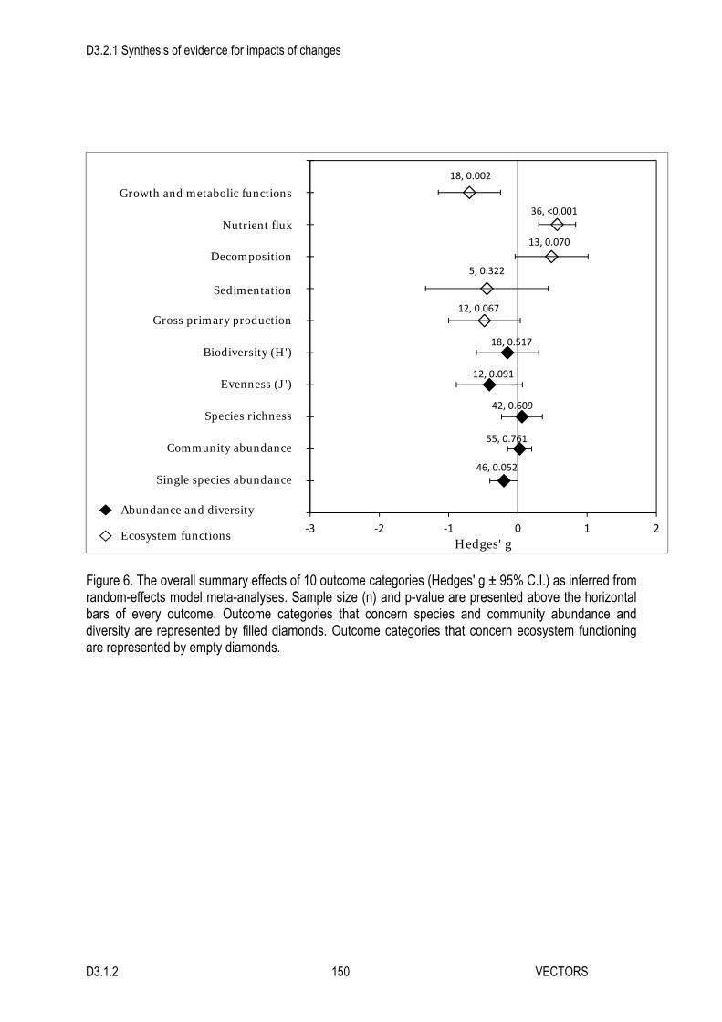
D3.2.1 Synthesis of evidence for impacts of changes  

D3.1.2 150 VECTORS

Figure 6. The overall summary effects of 10 outcome categories (Hedges' g ± 95% C.I.) as inferred from random-effects model meta-analyses. Sample size (n) and p-value are presented above the horizontal bars of every outcome. Outcome categories that concern species and community abundance and diversity are represented by filled diamonds. Outcome categories that concern ecosystem functioning are represented by empty diamonds.

55, 0.761

46, 0.052

42, 0.609

12, 0.091

18, 0.517

12, 0.067

5, 0.322

13, 0.070

36, <0.001

18, 0.002

‐3 ‐2 ‐1 0 1 2

Hedges' g

Abundance and diversity

Ecosystem functions

Growth and metabolic functions

Nutrient flux

Decomposition

Sedimentation

Species richness

Community abundance

Single species abundance

Gross primary production

Biodiversity (H')

Evenness (J')

D3.2.1 Synthesis of evidence for impacts of changes  

D3.1.2 151 VECTORS

Figure 7. Meta-analysis of single species abundance (n=46) using random-effects model to compute the summary effect size (Hedges' g ± 95% C.I.). The effect size of each study is represented by a black square symbol, which area is proportional to the study weight. The diamond at the bottom of the forest plot and its width represent the summary effect size ± 95% C.I.

Study name Statistics for each study Hedges's g and 95% CI

Hedges's g Variance p‐Value

Olabarria et al 2010 Site 1† 0.018 0.033 0.923

Lutz et al 2010 Towradgi† ‐0.052 0.129 0.884

Buttger et al 2008 ‐0.167 0.184 0.696

Ferrer et al 1997 Gracilaria 0.145 0.085 0.620

Wonham et al 2005 ‐0.236 0.225 0.619

Levin et al 2002 ‐0.129 0.067 0.617

Schwindt et al 2001 0.085 0.013 0.459

Holloway & Keough 2002a Outer Harbour† ‐0.079 0.008 0.386

Kotta et al 2001 ‐0.616 0.345 0.294

Malyshev & Quijon 2011 0.381 0.122 0.276

Markert et al 2009 ‐0.754 0.474 0.273

Olabarria et al 2010 Site 2† 0.236 0.037 0.218

O'Brien et al 2006 0.869 0.364 0.150

Holloway & Keough 2002a St Kilda† 0.142 0.008 0.120

Wright et al 2007 Burrill Lake† 0.315 0.035 0.092

Lutz et al 2010 Bulli† 0.655 0.119 0.057

Kochmann et al 2008 0.578 0.081 0.043

Vazquez‐Luis et al 2010 ‐0.938 0.185 0.029

Lorenti et al 2011 0.431 0.030 0.012

Ferrer et al 1997 Cystoseira ‐0.775 0.093 0.011

Sweetman et al 2010 Pearl harbour† 0.719 0.069 0.006

Crooks & Khim 1999 0.254 0.009 0.006

Irigoyen et al 2011 0.741 0.071 0.005

Sweetman et al 2010 Kaneohe bay† 1.188 0.178 0.005

Vazquez‐Luis et al 2009b 0.723 0.055 0.002

Chen el al 2007 ‐0.372 0.013 0.001

Hofle et al 2011 ‐0.496 0.024 0.001

Davis 1998 3.445 1.120 0.001

Windham & Ehrenfeld 2003 ‐2.756 0.706 0.001

Crooks 1998 0.985 0.088 0.001

Bruschetti et al 2009 0.453 0.018 0.001

Lang & Buschbaum 2010 ‐1.189 0.118 0.001

Holsman et al 2010 ‐1.287 0.133 0.000

Montefalcone et al 2007 ‐0.631 0.027 0.000

Wright et al 2010 ‐2.156 0.300 0.000

Lutz et al 2010 Gerringong† ‐1.795 0.168 0.000

Neideman et al 2003 ‐3.728 0.658 0.000

Wright et al 2007 St Georges Basin† ‐1.041 0.038 0.000

Sureda et al 2008 ‐7.151 1.462 0.000

Angradi et al 2001 ‐0.084 0.000 0.000

Heiman et al 2008 0.979 0.023 0.000

Chapman et al 2005 ‐1.640 0.042 0.000

Feyrer et al 2003 ‐0.776 0.009 0.000

Cottet et al 2007 1.763 0.021 0.000

Wright et al 2007 Lake Conjola† ‐1.208 0.021 0.000

Deudero et al 2010 ‐1.467 0.005 0.000

‐0.201 0.011 0.052

‐10.00 ‐5.00 0.00 5.00 10.00

D3.2.1 Synthesis of evidence for impacts of changes  

D3.1.2 152 VECTORS

Figure 8. Subgroup analyses of single species abundance by: A) study type, B) study settings, C) engineering type, D) invasive ecosystem engineer taxonomic group, E) habitat, and F) region. To compute each summary effect size (Hedges' g ± 95% C.I.) a mixed-effects model was used. A random effects model is used to combine studies within each subgroup. A fixed effect model is used to combine subgroups and yield the overall effect. The study-to-study variance (tau-squared) is assumed to be the same for all subgroups - this value is computed within subgroups and then pooled across subgroups.

Hedges' g

-1.0 -0.8 -0.6 -0.4 -0.2 0.0 0.2 0.4 0.6 0.8

Allogenic

Autogenic

Both

Overall

Hedges' g

-2.0 -1.5 -1.0 -0.5 0.0 0.5

Field

Lab

Overall

Hedges' g

-0.8 -0.6 -0.4 -0.2 0.0 0.2 0.4

Experimental

Observational

Overall

Hedges' g

-6 -4 -2 0 2 4 6 8

Artificial reef

Coral reef

Estuary

Harbour

Lagoons

Mangrove forest

Mudflat

Open coast

Oyster bed

Rocky intertidal

Rocky subtidal

Salt marsh

Sandy intertidal

Sandy subtidal

Seagrass meadow

Overall

Hedges' g

-3 -2 -1 0 1 2 3

Angiosperms

Annelida

Bivalvia

Chlorophyta

Crustacea

Gastropoda

Phaeophyta

Rhodophyta

Overall

Hedges' g

-8 -6 -4 -2 0 2 4

Baltic Sea

California Current

Celtic-Biscay Shelf

East China Sea

EC Australian Shelf

Gulf of California

Iberian Coastal

Insular Pacific-Hawaiian

Mediterranean

North Sea

NE U.S. Continental Shelf

Patagonian Shelf

Scotian Shelf

SE Australian Shelf

Overall

A B

C D

E

F

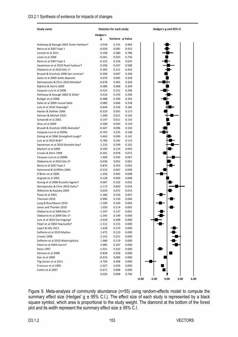
D3.2.1 Synthesis of evidence for impacts of changes  

D3.1.2 153 VECTORS

Figure 9. Meta-analysis of community abundance (n=55) using random-effects model to compute the summary effect size (Hedges' g ± 95% C.I.). The effect size of each study is represented by a black square symbol, which area is proportional to the study weight. The diamond at the bottom of the forest plot and its width represent the summary effect size ± 95% C.I.

Study name Statistics for each study Hedges's g and 95% CI

Hedges's g Variance p‐Value

Holloway & Keough 2002 Outer Harbour† 0.018 0.155 0.964

Neira et al 2007 Expt 1 ‐0.029 0.092 0.923

Lorenti et al 2011 0.168 0.380 0.786

Levin et al 2006 ‐0.061 0.033 0.736

Neira et al 2007 Expt 3 ‐0.225 0.226 0.635

Sweetman et al 2010 Pearl harbour† 0.358 0.437 0.588

Olabarria et al 2010 Site 1† 0.305 0.151 0.433

Brusa  & Grosholz 2006 San Lorenzo† ‐0.206 0.047 0.340

Zaiko et al 2009 shells deposits 0.070 0.005 0.328

Demopoulos & Chris 2010 Molokai† ‐0.678 0.465 0.320

Dijkstra & Harris 2009 0.089 0.008 0.304

Vazquez‐Luis et al 2008 ‐0.525 0.252 0.296

Holloway & Keough 2002 St Kilda† 0.416 0.159 0.296

Buttger et al 2008 ‐0.488 0.189 0.263

Zaiko et al 2009 mussel beds 0.085 0.006 0.258

Lutz et al 2010 Towradgi† 0.644 0.236 0.185

Hacker & Dethier 2006 ‐0.319 0.055 0.173

Heiman & Micheli 2010 1.096 0.621 0.164

Schwindt et al 2001 0.147 0.011 0.155

Zhou et al 2009 0.300 0.043 0.150

Brusa  & Grosholz 2006 Alameda† ‐0.447 0.096 0.150

Vazquez‐Luis et al 2009a ‐0.702 0.235 0.148

Strong et al 2006 Strangford Lough† 0.463 0.099 0.141

Lutz et al 2010 Bulli† 0.780 0.242 0.113

Sweetman et al 2010 Kaneohe bay† 1.210 0.549 0.102

Markert et al 2009 0.593 0.124 0.093

Crooks & Khim 1999 ‐0.501 0.078 0.072

Vazquez‐Luis et al 2009b 1.409 0.592 0.067

Olabarria et al 2010 Site 2† 0.430 0.052 0.061

Neira et al 2007 Expt 2 0.876 0.203 0.052

Hammond & Griffiths 2006 ‐0.510 0.067 0.049

O'Brien et al 2006 ‐1.256 0.405 0.048

Angradi et al 2001 0.128 0.004 0.048

Strong et al 2006 Russells lagoon† 0.687 0.102 0.032

Demopoulos & Chris 2010 Oahu†  2.172 0.820 0.016

Wikstrom & Kautsky 2004 0.659 0.072 0.014

Piazzi et al 2001 ‐1.360 0.256 0.007

Thomsen 2010 0.996 0.130 0.006

Lang & Buschbaum 2010 ‐1.509 0.269 0.004

Jones and Thorber 2010 1.020 0.114 0.002

Olabarria et al 2009 Site 2† ‐1.247 0.137 0.001

Olabarria et al 2009 Site 1† ‐1.345 0.149 0.000

Lutz et al 2010 Gerringong† ‐2.429 0.408 0.000

Floerl et al 2004 Townsville† ‐1.512 0.155 0.000

Lejart & Hily 2011 1.628 0.170 0.000

Sellheim et al 2010 Mytilus 1.475 0.119 0.000

Crooks 1998 2.142 0.251 0.000

Sellheim et al 2010 Watersiphora 1.480 0.119 0.000

Floerl et al 2004 Cairns† 2.085 0.187 0.000

Davis 1997 ‐1.551 0.102 0.000

Heiman et al 2008 0.838 0.028 0.000

Gan et al 2009 ‐0.419 0.006 0.000

Tlig‐Zouari et al 2011 ‐3.704 0.408 0.000

Francour et al 1995 ‐1.027 0.026 0.000

Cottet et al 2007 ‐0.671 0.008 0.000

0.026 0.008 0.766

‐6.00 ‐3.00 0.00 3.00 6.00

D3.2.1 Synthesis of evidence for impacts of changes  

D3.1.2 154 VECTORS

Figure 10. Subgroup analyses of community abundance by: A) study type, B) invasive ecosystem engineer taxonomic group, C) engineering type, D) region, and E) habitat. To compute each summary effect size (Hedges' g ± 95% C.I.) a mixed-effects model was used. A random effects model is used to combine studies within each subgroup. A fixed effect model is used to combine subgroups and yield the overall effect. The study-to-study variance (tau-squared) is assumed to be the same for all subgroups - this value is computed within subgroups and then pooled across subgroups.

Hedges' g

-1.5 -1.0 -0.5 0.0 0.5 1.0

Allogenic

Autogenic

Both

Overall

Hedges' g

-0.3 -0.2 -0.1 0.0 0.1 0.2 0.3 0.4 0.5

Experimental

Observational

Overall

Hedges' g

-4 -3 -2 -1 0 1 2 3

Artificial reefs

Coral reef

Estuary

Lagoon

Mangroves

Mudflat

Open coast

Oyster beds

Rocky intertidal

Rocky subtidal

Salt marshes

Sandflat

Seagrass meadow

Overall

Hedges' g

-1.5 -1.0 -0.5 0.0 0.5 1.0 1.5 2.0 2.5

Angiosperms

Annelida

Bivalvia

Bryozoa

Chlorophyta

Phaeophyta

Rhodophyta

Tunicata

Overall

Hedges' g

-2 -1 0 1 2

Baltic Sea

Benguela current

California Current

Celtic-Biscay Shelf

East China Sea

EC Australian Shelf

Gulf of Alaska

Gulf of California

Iberian Coastal

Insular Pacific-Hawaiian

Mediterranean

North Sea

NE Australian Shelf

NE U.S. Continental Shelf

Patagonian Shelf

SE Australia

Overall

A

C

B

E

D

D3.2.1 Synthesis of evidence for impacts of changes  

D3.1.2 155 VECTORS

Figure 11. Meta-analysis of species richness (n=42) using random-effects model to compute the summary effect size (Hedges' g ± 95% C.I.). The effect size of each study is represented by a black square symbol, which area is proportional to the study weight. The diamond at the bottom of the forest plot and its width represent the summary effect size ± 95% C.I.

Study name Statistics for each study Hedges's g and 95% CI

Hedges's g Variance p‐Value

Cottet et al 2007 0.028 0.771 0.974

Lutz et al 2010 Bulli† ‐0.028 0.223 0.952

Vazquez‐Luis et al 2009a 0.043 0.236 0.930

Chen el al 2007 0.080 0.284 0.880

Hammond & Griffiths 2006 ‐0.044 0.065 0.864

Strong et al 2006 Strangford Lough† ‐0.084 0.096 0.786

Lutz et al 2010 Gerringong† ‐0.147 0.224 0.756

Lutz et al 2010 Towradgi† ‐0.201 0.225 0.672

Demopoulos & Chris 2010 Molokai† 0.320 0.435 0.628

Mineur et al 2008 Ireland† 0.069 0.018 0.609

Neira et al 2007 Expt 1 0.225 0.185 0.601

Thomsen 2010 0.197 0.117 0.564

Lorenti et al 2011 ‐0.464 0.392 0.458

Drouin et al 2011 Fish Grosse Iles† 0.165 0.041 0.415

Olabarria et al 2010 Site 2† ‐0.365 0.148 0.343

Olabarria et al 2009 Site 1† ‐0.573 0.343 0.328

Vazquez‐Luis et al 2008 ‐0.584 0.301 0.287

Drouin et al 2011 Fish Old Hurry† 0.232 0.041 0.253

Olabarria et al 2010 Site 1† ‐0.548 0.151 0.159

Jones and Thorber 2010 0.460 0.103 0.151

Strong et al 2006 Russells lagoon† 0.464 0.099 0.140

Sellheim et al 2010 Watersiphora 0.664 0.152 0.088

Demopoulos & Chris 2010 Oahu†  1.834 0.707 0.029

Crooks & Khim 1999 1.194 0.268 0.021

Buschbaum et al 2006 Helgoland† ‐1.233 0.271 0.018

Vazquez‐Luis et al 2009b 2.522 0.957 0.010

Mineur et al 2008 England† ‐0.357 0.019 0.009

Lang & Buschbaum 2010 ‐2.455 0.755 0.005

Dijkstra & Harris 2009 Expt 1 0.247 0.008 0.005

Olabarria et al 2009 Site 2† ‐2.424 0.620 0.002

Piazzi et al 2001 ‐3.933 1.496 0.001

Neira et al 2007 Expt 2 1.613 0.249 0.001

Dijkstra & Harris 2009 Expt 2 ‐0.812 0.060 0.001

Buschbaum et al 2006 Sylt† 1.722 0.258 0.001

Crooks 1998 1.862 0.228 0.000

Drouin et al 2011 Expt1 0.618 0.022 0.000

Sellheim et al 2010 Mytilus 1.539 0.134 0.000

Neira et al 2007 Expt 3 ‐4.428 1.101 0.000

Francour et al 1995 ‐1.072 0.026 0.000

Tlig‐Zouari et al 2011 ‐18.806 7.117 0.000

Angradi et al 2001 ‐0.982 0.016 0.000

Lejart & Hily 2011 7.011 0.553 0.000

0.059 0.023 0.693

‐10.00 ‐5.00 0.00 5.00 10.00

D3.2.1 Synthesis of evidence for impacts of changes  

D3.1.2 156 VECTORS

Figure 12. Subgroup analyses of species richness by: A) study type, B) invasive ecosystem engineer taxonomic group, C) engineering type, D) region, and E) habitat. To compute each summary effect size (Hedges' g ± 95% C.I.) a mixed-effects model was used. A random effects model is used to combine studies within each subgroup. A fixed effect model is used to combine subgroups and yield the overall effect. The study-to-study variance (tau-squared) is assumed to be the same for all subgroups - this value is computed within subgroups and then pooled across subgroups.

Hedges' g

-0.8 -0.6 -0.4 -0.2 0.0 0.2 0.4 0.6

Experimental

Observational

Overall

Hedges' g

-1.0 -0.8 -0.6 -0.4 -0.2 0.0 0.2 0.4 0.6 0.8 1.0

Allogenic

Autogenic

Both

Overall

Hedges' g

-2 -1 0 1 2 3

Angiosperms

Bivalvia

Bryozoa

Chlorophyta

Phaeophyta

Rhodophyta

Tunicata

Overall

Hedges' g

-6 -4 -2 0 2 4

Estuary

Lagoon

Mangrove forest

Mudflat

Oyster bed

Rocky intertidal

Rocky subtidal

Salt marsh

Seagrass meadow

Tidal sandflat

Overall

Hedges' g

-3 -2 -1 0 1 2 3 4

Benguela current

California Current

Celtic-Biscay Shelf

East China Sea

EC Australia

Gulf of California

Iberian Coastal

Insular Pacific-Hawaiian

Mediterranean

North Sea

NE U.S. Shelf

Scotian Shelf

Overall

A B

C

D

E

D3.2.1 Synthesis of evidence for impacts of changes  

D3.1.2 157 VECTORS

Figure 13. Meta-analysis of species diversity (n=18) using random-effects model to compute the summary effect size (Hedges' g ± 95% C.I.). The weight of each study is represented by its square size. The effect size of each study is represented by a black square symbol, which area is proportional to the study weight. The diamond at the bottom of the forest plot and its width represent the summary effect size ± 95% C.I.

Study name Statistics for each study Hedges's g and 95% CI

Hedges's g Variance p‐Value

Neira et al 2007 Expt 1 0.035 0.183 0.935

Strong et al 2006 Russells lagoon† 0.039 0.096 0.900

Chen el al 2007 0.088 0.297 0.871

Lorenti et al 2011 ‐0.231 0.381 0.709

Drouin et al 2011 Invertebrates 0.080 0.021 0.576

Hammond & Griffiths 2006 0.228 0.065 0.373

Irigoyen et al 2011 0.673 0.349 0.254

Demopoulos & Chris 2010 Oahu† 0.792 0.479 0.252

Neira et al 2007 Expt 2 0.667 0.195 0.131

Drouin et al 2011 Fish Old Hurry† 0.389 0.042 0.057

Strong et al 2006 Strangford Lough† ‐0.735 0.103 0.022

Demopoulos & Chris 2010 Molokai† ‐2.144 0.810 0.017

Neira et al 2007 Expt 3 ‐2.081 0.464 0.002

Sellheim et al 2010 Mytilus 1.079 0.108 0.001

Drouin et al 2011 Fish Grosse Iles† 0.716 0.044 0.001

Piazzi et al 2001 ‐3.961 1.199 0.000

Sellheim et al 2010 Watersiphora 1.429 0.129 0.000

Tlig‐Zouari et al 2011 ‐9.823 2.017 0.000

‐0.149 0.053 0.517

‐15.00 ‐7.50 0.00 7.50 15.00

D3.2.1 Synthesis of evidence for impacts of changes  

D3.1.2 158 VECTORS

Hedges' g

-1.5 -1.0 -0.5 0.0 0.5 1.0 1.5 2.0

Allogenic

Autogenic

Both

Overall

Hedges' g

-1.5 -1.0 -0.5 0.0 0.5 1.0 1.5

Experimental

Observational

Overall

Hedges' g

-3 -2 -1 0 1 2 3

Lagoon

Mangroves

Mudflat

Rocky intertidal

Seagrass meadow

Tidal sandflat

Overall

Hedges' g

-4 -3 -2 -1 0 1 2 3 4

Angiosperms

Bivalvia

Bryozoa

Chlorophyta

Phaeophyta

Overall

Hedges' g

-6 -4 -2 0 2 4

Benguela current

California Current

Celtic-Biscay Shelf

East China Sea

Insular Pacific-Hawaiian

Mediterranean

Patagonian Shelf

Scotian Shelf

Overall

A B

C D

E

Figure 14. Subgroup analyses of species diversity by: A) study type, B) engineering type, C) invasive ecosystem engineer taxonomic group, D) habitat, and E) region. To compute each summary effect size (Hedges' g ± 95% C.I.) a mixed-effects model was used. A random effects model is used to combine studies within each subgroup. A fixed effect model is used to combine subgroups and yield the overall effect. The study-to-study variance (tau-squared) is assumed to be the same for all subgroups - this value is computed within subgroups and then pooled across subgroups. .

D3.2.1 Synthesis of evidence for impacts of changes  

D3.1.2 159 VECTORS

Figure 15. Meta-analysis of species evenness (n=12) using random-effects model to compute the summary effect size (Hedges' g ± 95% C.I.). The effect size of each study is represented by a black square symbol, which area is proportional to the study weight. The diamond at the bottom of the forest plot and its width represent the summary effect size ± 95% C.I.

Study name Statistics for each study Hedges's g and 95% CI

Hedges's g Variance p‐Value

Demopoulos & Chris 2010 Oahu† ‐0.408 0.441 0.539

Demopoulos & Chris 2010 Molokai† ‐3.168 1.263 0.005

Lorenti et al 2012 0.202 0.381 0.743

Neira et al 2007 Expt 1 0.000 0.183 1.000

Neira et al 2007 Expt 2 ‐0.110 0.184 0.798

Neira et al 2007 Expt 3 ‐0.470 0.293 0.385

Strong et al 2006 Strangford Lough† ‐0.260 0.097 0.403

Strong et al 2006 Russells lagoon† ‐0.373 0.098 0.233

Tlig‐Zouari et al 2011 ‐4.493 0.501 0.000

Drouin et al 2011 Invertebrates ‐0.227 0.021 0.115

Drouin et al 2011 Fish Old Hurry† 0.285 0.041 0.162

Drouin et al 2011 Fish Grosse Iles† 0.696 0.044 0.001

‐0.411 0.059 0.092

‐25.00 ‐12.50 0.00 12.50 25.00

D3.2.1 Synthesis of evidence for impacts of changes  

D3.1.2 160 VECTORS

Figure 16. Subgroup analyses of species evenness by: A) study type, B) engineering type, C) invasive ecosystem engineer taxonomic group, D) habitat, and E) region. To compute each summary effect size (Hedges' g ± 95% C.I.) a mixed-effects model was used. A random effects model is used to combine studies within each subgroup. A fixed effect model is used to combine subgroups and yield the overall effect. The study-to-study variance (tau-squared) is assumed to be the same for all subgroups - this value is computed within subgroups and then pooled across subgroups.

Hedges' g

-3 -2 -1 0 1 2

Allogenic

Autogenic

Both

Overall

Hedges' g

-1.5 -1.0 -0.5 0.0 0.5 1.0

Experimental

Observational

Overall

Hedges' g

-2 -1 0 1 2 3

Angiosperms

Bivalvia

Chlorophyta

Phaeophyta

Overall

Hedges' g

-4 -3 -2 -1 0 1 2 3

Lagoon

Mangrove forest

Mudflat

Rocky intertidal

Tidal sandflat

Overall

Hedges' g

-4 -3 -2 -1 0 1 2

California Current

Celtic-Biscay Shelf

Insular Pacific-Hawaiian

Mediterranean

Scotian Shelf

Overall

A B

C D

E

D3.2.1 Synthesis of evidence for impacts of changes  

D3.1.2 161 VECTORS

Figure 17. Meta-analysis of gross primary production (n=12) using random-effects model to compute the summary effect size (Hedges' g ± 95% C.I.). The effect size of each study is represented by a black square symbol, which area is proportional to the study weight. The diamond at the bottom of the forest plot and its width represent the summary effect size ± 95% C.I.

Study name Statistics for each study Hedges's g and 95% CI

Hedges's g Variance p‐Value

Olabarria et al 2010 Site 1† ‐0.082 0.098 0.793

Kotta et al 2001 0.320 0.112 0.340

Olabarria et al 2010 Site 2† ‐0.313 0.098 0.317

Wonham et al 2005 ‐0.960 0.252 0.056

Bruschetti et al 2008  ‐0.703 0.122 0.044

Neira et al 2007 Expt 2 ‐0.996 0.208 0.029

Larned 2003 ‐0.686 0.073 0.011

Neira et al 2007 Expt 1 ‐1.297 0.226 0.006

Neira et al 2007 Expt 3 2.699 0.587 0.000

Deudero et al 2011 ‐1.344 0.131 0.000

Bruschetti et al 2011 ‐2.902 0.551 0.000

Nasrollahzadeh et al 2008a 0.405 0.008 0.000

‐0.483 0.070 0.067

‐6.00 ‐3.00 0.00 3.00 6.00

D3.2.1 Synthesis of evidence for impacts of changes  

D3.1.2 162 VECTORS

Hedges' g

-3.5 -3.0 -2.5 -2.0 -1.5 -1.0 -0.5 0.0 0.5

Allogenic

Autogenic

Both

Overall

Hedges' g

-2.0 -1.5 -1.0 -0.5 0.0 0.5

Experimental

Observational

Overall

Hedges' g

-4 -3 -2 -1 0 1 2

Estuary

Lagoon

Mudflat

Open coast

Seagrass meadow

Tidal sandflat

Overall

Hedges' g

-4 -3 -2 -1 0 1 2

Angiosperms

Annelida

Chlorophyta

Ctenophora

Gastropoda

Phaeophyta

Overall

Hedges' g

-4 -3 -2 -1 0 1 2 3

California Current

Caspian Sea

Iberian Coastal

Mediterranean

North Sea

Patagonian Shelf

Overall

A B

C D

E

D3.2.1 Synthesis of evidence for impacts of changes  

D3.1.2 163 VECTORS

Figure 18. Subgroup analyses of gross primary production by: A) study type, B) engineering type, C) invasive ecosystem engineer taxonomic group, D) habitat, and E) region. To compute each summary effect size (Hedges' g ± 95% C.I.) a mixed-effects model was used. A random effects model is used to combine studies within each subgroup. A fixed effect model is used to combine subgroups and yield the overall effect. The study-to-study variance (tau-squared) is assumed to be the same for all subgroups - this value is computed within subgroups and then pooled across subgroups.

Figure 19. Meta-analysis of sedimentation (n=5) using random-effects model to compute the summary effect size (Hedges' g ± 95% C.I.). The effect size of each study is represented by a black square symbol, which area is proportional to the study weight. The diamond at the bottom of the forest plot and its width represent the summary effect size ± 95% C.I.

Study name Statistics for each study Hedges's g and 95% CI

Hedges's g Variance p‐Value

Holmer et al 2009 Caulerpa prolifera 0.516 0.340 0.376

Holmer et al 2009 Caulerpa racemosa ‐1.661 0.464 0.015

Holmer et al 2009 Caulerpa taxifolia ‐1.977 0.522 0.006

Neira et al 2007 Expt 3 ‐0.271 0.185 0.529

Hacker & Dethier 2006 0.413 0.008 0.000

‐0.447 0.205 0.323

‐4.00 ‐2.00 0.00 2.00 4.00

D3.2.1 Synthesis of evidence for impacts of changes  

D3.1.2 164 VECTORS

Figure 20. Subgroup analyses of sedimentation by: A) study type, B) engineering type, C) invasive ecosystem engineer taxonomic group, and D) region. To compute each summary effect size (Hedges' g ± 95% C.I.) a mixed-effects model was used. A random effects model is used to combine studies within each subgroup. A fixed effect model is used to combine subgroups and yield the overall effect. The study-to-study variance (tau-squared) is assumed to be the same for all subgroups - this value is computed within subgroups and then pooled across subgroups.

Hedges' g

-3 -2 -1 0 1 2 3

Allogenic

Autogenic

Overall

Hedges' g

-2.5 -2.0 -1.5 -1.0 -0.5 0.0 0.5 1.0 1.5

Experimental

Observational

Overall

Hedges' g

-2.5 -2.0 -1.5 -1.0 -0.5 0.0 0.5 1.0 1.5

Angiosperms

Chlorophyta

Overall

Hedges' g

-4 -3 -2 -1 0 1 2 3 4

California Current

Gulf of Alaska

Mediterranean

Overall

A B

C D

D3.2.1 Synthesis of evidence for impacts of changes  

D3.1.2 165 VECTORS

Figure 21. Meta-analysis of decomposition (n=13) using random-effects model to compute the summary effect size (Hedges' g ± 95% C.I.). The effect size of each study is represented by a black square symbol, which area is proportional to the study weight. The diamond at the bottom of the forest plot and its width represent the summary effect size ± 95% C.I.

Study name Statistics for each study Hedges's g and 95% CI

Hedges's g Variance p‐Value

Holmer et al 2009 C. racemosa ‐0.048 0.427 0.942

Bruschetti et al 2011  0.336 0.101 0.290

Holmer et al 2009 C. taxifolia ‐0.792 0.479 0.252

Olabarria et al 2010 Site 1† ‐0.501 0.149 0.195

Crooks & Khim 1999 0.719 0.240 0.142

Olabarria et al 2010 Site 2† 0.620 0.153 0.113

Neira et al 2007 Expt 1 ‐0.787 0.199 0.077

Neira et al 2007 Expt 2 ‐1.097 0.214 0.018

Holmer et al 2009 C. prolifera 2.428 0.918 0.011

Hahn 2003  1.403 0.203 0.002

Neira et al 2007 Expt 3 2.312 0.507 0.001

Cottet et al 2007 0.916 0.044 0.000

Kristensen et al 2011 1.540 0.077 0.000

0.487 0.072 0.070

‐5.00 ‐2.50 0.00 2.50 5.00

D3.2.1 Synthesis of evidence for impacts of changes  

D3.1.2 166 VECTORS

Figure 22. Subgroup analyses of decomposition by: A) study type, B) engineering type, C) invasive ecosystem engineer taxonomic group, D) habitat, and E) region. To compute each summary effect size (Hedges' g ± 95% C.I.) a mixed-effects model was used. A random effects model is used to combine studies within each subgroup. A fixed effect model is used to combine subgroups and yield the overall effect. The study-to-study variance (tau-squared) is assumed to be the same for all subgroups - this value is computed within subgroups and then pooled across subgroups.

Hedges' g

-1.0 -0.5 0.0 0.5 1.0 1.5 2.0 2.5

Allogenic

Autogenic

Both

Overall

Hedges' g

-1.0 -0.5 0.0 0.5 1.0 1.5 2.0

Experimental

Observational

Overall

Hedges' g

-2 -1 0 1 2 3 4

Angiosperms

Annelida

Bivalvia

Chlorophyta

Phaeophyta

Overall

Hedges' g

-3 -2 -1 0 1 2 3 4

Estuary

Lagoon

Seagrass meadow

Tidal sandflat

Overall

Hedges' g

-3 -2 -1 0 1 2 3 4 5

California Current

Celtic-Biscay Shelf

Gulf of Alaska

Gulf of California

Iberian Coastal

Mediterranean

North Sea

Patagonian Shelf

Overall

A B

C D

E

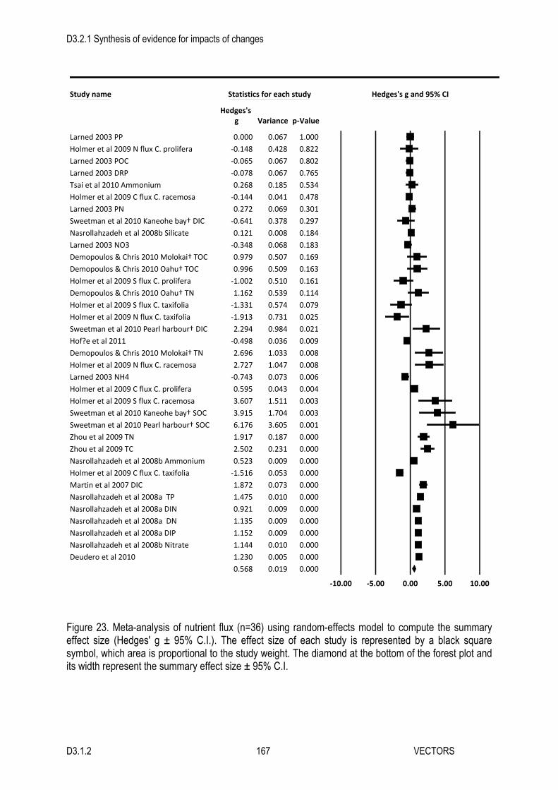
D3.2.1 Synthesis of evidence for impacts of changes  

D3.1.2 167 VECTORS

Figure 23. Meta-analysis of nutrient flux (n=36) using random-effects model to compute the summary effect size (Hedges' g ± 95% C.I.). The effect size of each study is represented by a black square symbol, which area is proportional to the study weight. The diamond at the bottom of the forest plot and its width represent the summary effect size ± 95% C.I.

Study name Statistics for each study Hedges's g and 95% CI

Hedges's g Variance p‐Value

Larned 2003 PP 0.000 0.067 1.000

Holmer et al 2009 N flux C. prolifera ‐0.148 0.428 0.822

Larned 2003 POC ‐0.065 0.067 0.802

Larned 2003 DRP ‐0.078 0.067 0.765

Tsai et al 2010 Ammonium 0.268 0.185 0.534

Holmer et al 2009 C flux C. racemosa ‐0.144 0.041 0.478

Larned 2003 PN 0.272 0.069 0.301

Sweetman et al 2010 Kaneohe bay† DIC ‐0.641 0.378 0.297

Nasrollahzadeh et al 2008b Silicate 0.121 0.008 0.184

Larned 2003 NO3 ‐0.348 0.068 0.183

Demopoulos & Chris 2010 Molokai† TOC 0.979 0.507 0.169

Demopoulos & Chris 2010 Oahu† TOC 0.996 0.509 0.163

Holmer et al 2009 S flux C. prolifera ‐1.002 0.510 0.161

Demopoulos & Chris 2010 Oahu† TN 1.162 0.539 0.114

Holmer et al 2009 S flux C. taxifolia ‐1.331 0.574 0.079

Holmer et al 2009 N flux C. taxifolia ‐1.913 0.731 0.025

Sweetman et al 2010 Pearl harbour† DIC 2.294 0.984 0.021

Hof?e et al 2011 ‐0.498 0.036 0.009

Demopoulos & Chris 2010 Molokai† TN 2.696 1.033 0.008

Holmer et al 2009 N flux C. racemosa 2.727 1.047 0.008

Larned 2003 NH4 ‐0.743 0.073 0.006

Holmer et al 2009 C flux C. prolifera 0.595 0.043 0.004

Holmer et al 2009 S flux C. racemosa 3.607 1.511 0.003

Sweetman et al 2010 Kaneohe bay† SOC 3.915 1.704 0.003

Sweetman et al 2010 Pearl harbour† SOC 6.176 3.605 0.001

Zhou et al 2009 TN 1.917 0.187 0.000

Zhou et al 2009 TC 2.502 0.231 0.000

Nasrollahzadeh et al 2008b Ammonium 0.523 0.009 0.000

Holmer et al 2009 C flux C. taxifolia ‐1.516 0.053 0.000

Martin et al 2007 DIC 1.872 0.073 0.000

Nasrollahzadeh et al 2008a  TP 1.475 0.010 0.000

Nasrollahzadeh et al 2008a DIN 0.921 0.009 0.000

Nasrollahzadeh et al 2008a  DN 1.135 0.009 0.000

Nasrollahzadeh et al 2008a DIP 1.152 0.009 0.000

Nasrollahzadeh et al 2008b Nitrate 1.144 0.010 0.000

Deudero et al 2010 1.230 0.005 0.000

0.568 0.019 0.000

‐10.00 ‐5.00 0.00 5.00 10.00

D3.2.1 Synthesis of evidence for impacts of changes  

D3.1.2 168 VECTORS

Hedges' g

-0.5 0.0 0.5 1.0 1.5 2.0 2.5 3.0

Allogenic

Autogenic

Both

OverallHedges' g

-0.5 0.0 0.5 1.0 1.5

Experimental

Observational

Overall

Hedges' g

-3 -2 -1 0 1 2 3 4

Angiosperms

Chlorophyta

Ctenophora

Gastropoda

Rhodophyta

Overall

Hedges' g

-2 -1 0 1 2 3 4

Estuary

Mangroves

Open coast

Salt marsh

Seagrass meadow

Tidal sandflat

Overall

Hedges' g

-3 -2 -1 0 1 2 3 4

California Current

Caspian Sea

Celtic-Biscay Shelf

East China Sea

Insular Pacific-Hawaiian

Mediterranean

North Sea

NE U.S. Shelf

Overall

A B

C

D

E

Hedges' g

-1.5 -1.0 -0.5 0.0 0.5 1.0 1.5 2.0

Carbon

Nitrogen

Phosphorus

Sulfur

Silicate

Overall

Hedges' g

-1 0 1 2

Organic

Inorganic

Overall

E

F

G

Figure 24. Subgroup analyses of nutrient flux by: A) study type, B) engineering type, C) invasive ecosystem engineer taxonomic group, D) habitat, E) nutrient type, F) Nutrient identity, and G) region. To compute each summary effect size (Hedges' g ± 95% C.I.) a mixed-effects model was used. A random effects model is used to combine studies within each subgroup. A fixed effect model is used to combine subgroups and yield the overall effect. The study-to-study variance (tau-squared) is assumed to be the same for all subgroups - this value is computed within subgroups and then pooled across subgroups.

D3.2.1 Synthesis of evidence for impacts of changes  

D3.1.2 169 VECTORS

Figure 25. Meta-analysis of growth and metabolic functions (n=18) using random-effects model to compute the summary effect size (Hedges' g ± 95% C.I.). The effect size of each study is represented by a black square symbol, which area is proportional to the study weight. The diamond at the bottom of the forest plot and its width represent the summary effect size ± 95% C.I.

Study name Statistics for each study Hedges's g and 95% CI

Hedges's g Variance p‐Value

Levin et al 2002 ‐0.150 0.202 0.739

Strong et al 2006 Russells lagoon† ‐0.126 0.096 0.685

Markert et al 2009 ‐0.453 0.444 0.496

Holloway & Keough 2002b ‐0.299 0.144 0.430

Martin et al 2007 Alkalinity ‐0.213 0.045 0.316

Kotta et al 2001 0.601 0.344 0.306

Brusati & Grosholz 2007 ‐0.554 0.140 0.140

Hoffle et al 2011 ‐0.406 0.035 0.030

Sweetman et al 2010 Pearl harbour† ‐2.090 0.791 0.019

Reusch & Williams 1998 ‐1.616 0.457 0.017

Sweetman et al 2010 Kaneohe bay† 3.754 1.601 0.003

Vazquez‐Luis et al 2010 ‐3.452 0.922 0.000

Strong et al 2006 Strangford Lough† ‐1.239 0.115 0.000

Wright et al 2008 ‐1.941 0.278 0.000

Martin et al 2007 CaCO3 precipitation‐2.245 0.320 0.000

Deudero et al 2010 1.408 0.073 0.000

Eastwood et al 2007 ‐2.500 0.162 0.000

Feyrer et al 2003 ‐0.840 0.009 0.000

‐0.700 0.053 0.002

‐10.00 ‐5.00 0.00 5.00 10.00

D3.2.1 Synthesis of evidence for impacts of changes  

D3.1.2 170 VECTORS

Figure 26. Subgroup analyses of growth and metabolic functions by: A) study type, B) study settings, C) engineering type, D) invasive ecosystem engineer taxonomic group, E) habitat, and F) region. To compute each summary effect size (Hedges' g ± 95% C.I.) a mixed-effects model was used. A random effects model is used to combine studies within each subgroup. A fixed effect model is used to combine subgroups and yield the overall effect. The study-to-study variance (tau-squared) is assumed to be the same for all subgroups - this value is computed within subgroups and then pooled across subgroups.

Hedges' g

-2.0 -1.5 -1.0 -0.5 0.0 0.5 1.0 1.5

Allogenic

Autogenic

Both

Overall

Hedges' g

-2.5 -2.0 -1.5 -1.0 -0.5 0.0 0.5

Field

Lab

Overall

Hedges' g

-1.6 -1.4 -1.2 -1.0 -0.8 -0.6 -0.4 -0.2 0.0 0.2 0.4

Experimental

Observational

Overall

Hedges' g

-4 -3 -2 -1 0 1 2 3

Angiosperms

Annelida

Bivalvia

Chlorophyta

Crustacea

Gastropoda

Phaeophyta

Rhodophyta

Overall

Hedges' g

-5 -4 -3 -2 -1 0 1 2 3

Artificial reef

Estuary

Lagoon

Mangroves

Mudflat

Rocky intertidal

Rocky subtidal

Seagrass meadow

Tidal sandflat

Overall

Hedges' g

-5 -4 -3 -2 -1 0 1 2 3

California Current

Celtic-Biscay Shelf

Iberian Coastal

Insular Pacific-Hawaiian

Mediterranean

North Sea

NE U.S. Continental Shelf

SE Australia

SE U.S. Continental Shelf

Overall

A B

C D

E F

D3.2.1 Synthesis of evidence for impacts of changes  

D3.1.2 171 VECTORS

Figure 27.Funnel plots of standard error by Hedges' g, of the following outcomes: A) single-species abundance, B) community abundance, C) species richness, D) species diversity, E) species evenness, F) gross primary production, G) sedimentation H) decomposition, I) nutrient flux, and J) growth and metabolic functions. The observed studies are shown as open circles and the observed point estimates are shown as open diamonds below the x-axis. The imputed studies and adjusted point estimates according to the Trim and Fill algorithm (Duval and Tweedie 2000) are shown in filled circles and diamonds.

A B C

D E F

G H

J

I

D3.2.1 Synthesis of evidence for impacts of changes  

D3.1.2 172 VECTORS

Figure 28: Forest plot detailing effect sizes of invasive Spartina on the abundance of single species and taxonomic groups based on data published in Neira et al. (2007). This data exemplifies the high variability of effect sizes, varying between species and experiments, thus possibly obscuring valuable information when summarizing single effects into one overall effect size.

Hedges' g

-6 -4 -2 0 2 4

Tubificoides spp.Tectidrilus diversus

Monophylephorus evertusEnchytraeidae

Pseudopolydora kempiPolydora nuchalisPolydora cornuta

Streblospio benedictiPygospio elegans

Boccardia proboscideaHeteromastus filiformis

Capitella spp.Eteone californica

Eteone dilataeSphaerosyllis californiensis

Exogone loureiFabricia spp.

Nereis succineaTharyx sp.

Goniadidae sp.Dorvillea sp.

Mya arenariaMacoma petalumGemma gemma

Venerupis philippinarumMusculista senhousia

Corophium spp.Amphithoe valida

Grandidierella japonicaHyale sp.

Traskorchestia traskianaExosphaeroma inornata

TanaidaceaCumacea

Dolichopodidae larvaeChironomidae larvae

Ceratopogonidae larvaePoduridae

Psychodidae larvaeCanacidae larvae

Muscidae larveAnthozoa

TurbellariaOverall

Expt 1 – Mature vs. DiebackExpt 2 – Mature vs. ClippedExpt 3a – Mature vs. Un-invadedExpt 3b – Mature vs. Dieback

D3.2.1 Synthesis of evidence for impacts of changes  

D3.1.2 173 VECTORS

Figure 29. A conceptual model suggesting four pathways (numbered in the arrows delineated by double lines) through which invasive ecosystem engineers (mainly plants and sessile invertebrates with complex 3D structure) may affect ecosystem functions tested in this review and the ecological community. A description of the model is in the text.

Annex 1: Search terms used to find relevant studies We searched for relevant studies in Web of Science and Scopus online databases using three complex sets search terms. To identity studies involving invasive ecosystem engineering species ('exposure' set) we used search terms:

(("alien species" OR "alien organism*" OR "invasive species" OR "invasive organism*" OR "species invasion" OR "introduced species" OR "introduced organism*" OR "species introduced" OR "species introduction" OR "allochthonous species" OR "nonindigenous species" OR "non-indigenous species" OR "nonindigenous organism*" OR "non-indigenous organism*" OR "non native species" OR "non-native species" OR "non-native organism*" OR "exotic species" OR bioinvaion OR "bioinvasive species" OR "bioinvasive organism*") OR (“ecosystem engineer*”OR "bioconstruct*" OR “habitat modif*" OR "autogenic" OR "allogenic"))

This set was combined with a second set ('population') intended to isolate marine and estuarine studies and their associated biota:

(("marine" OR "brackish" OR "estuar*" OR "coastal" OR "shallow" OR "sea" OR "seas" OR "maritime" OR "lagoon*" OR "pelagic" OR "benth*" OR "demersal" OR "shore*" OR "intertidal" OR "subtidal" OR "ocean*" OR "bay" OR "cove") AND ("fauna*" OR "animal" OR "infauna*" OR "epifauna*" OR "fish" OR "macroinvertebrate" OR "invertebrate" OR "macrofauna*" OR "mesofauna*" OR "meiofauna*" OR "epibenthic" OR "seagrass" OR

D3.2.1 Synthesis of evidence for impacts of changes  

D3.1.2 174 VECTORS

"eelgrass" OR "cymodocea" OR "zostera" OR "posidonia" OR "seaweed" OR "macroalgal" OR "macroalgae" OR "fish*" OR "bird*" OR "seabird" OR "shorebird"))

This was combined with a third set ('outcome'), aimed to identify studies that had an effect on ecosystem structure and functioning:

(("species richness" OR diversity OR "community structure" OR evenness OR biodiversity OR bio-diversity OR "biological diversity" OR "Shannon-Weaver" OR "Shannon-Weiner" OR "Shannon index" OR "Simpson Index" OR "abundance-biomass curve*" OR "species abundance distribution*" OR "community similarity" OR "community dissimilarity") OR ("Energy flow*" OR "Energy flux*"OR "Flow* of energy" OR "Flux* of energy" OR biogeochemical OR "Nutrient cycl*" OR "cycling of nutrient*" OR "Nutrient dynamics" OR "nutrient flux*" OR "Nutrient flow*" OR "Flow* of nutrient*" OR "Flux* of nutrient*" OR "cycling of carbon" OR "carbon cycl*" OR "carbon stor*" OR "carbon flow*" OR "carbon flux*" OR "flow* of carbon" OR "flux* of carbon" OR "cycling of sul*ur" OR "Sul*ur cycl*" OR "Flow* of sul*ur" OR "flux* of sul*ur" OR "sul*ur flux*" OR"sul*ur flow*" OR "Hydrogen sul*ide" OR "cycling of nitrogen" OR "nitrogen cycl*" OR "Flow* of nitrogen" OR "flux* of nitrogen" OR "nitrogen flux*" OR "nitrogen flow*" OR denitrification OR "cycling of phosphorus"OR " phosphorus cycl*" OR "Flow* of phosphorus" OR "flux* of phosphorus" OR "phosphorus flux*" OR "phosphorus flow*"OR "cycling of oxygen" OR “oxygen cycl*" OR "Flow* of oxygen" OR "flux* of oxygen" OR "oxygen flux*" OR "oxygen flow*" OR anoxi* OR hypoxi* OR bioturbation OR grazing OR foraging OR herbivory OR predation OR scavengers OR scavenging OR respiration OR ecosystem metabolism OR "sediment stabilisation" OR "sediment mixing" ) OR (primary product*" OR "secondary product*" OR "carbon fixation" OR "community respiration" OR "ecosystem respiration" OR "community metabolism" OR "ecosystem metabolism" OR "abundance of benthic" OR "productivity of benthic" OR "benthic biomass" OR "biomass of benthic" OR "benthic metabolism" OR "benthic respiration" OR ((abundance* OR biomass* OR productivity OR mortalit* OR survival OR growth OR cover OR densit*))

Annex 2: Publications included in the meta-analysis

Angradi, T. R., S. M. Hagan, and K. W. Able. 2001. Vegetation type and the intertidal macroinvertebrate fauna of a brackish marsh: Phragmites vs. Spartina. Wetlands 21:75-92.

Brusati, E. D. and E. D. Grosholz. 2006. Native and introduced ecosystem engineers produce contrasting effects on estuarine infaunal communities. Biological Invasions 8:683-695.

Brusati, E. D. and E. D. Grosholz. 2007. Effect of native and invasive cordgrass on Macoma petalum density, growth, and isotopic signatures. Estuarine, Coastal and Shelf Science 71:517-522.

Bruschetti, M., C. Bazterrica, E. Fanjul, T. Luppi, and O. Iribarne. 2011. Effect of biodeposition of an invasive polychaete on organic matter content and productivity of the sediment in a coastal lagoon. Journal of Sea Research 66:20-28.

Bruschetti, M., C. Bazterrica, T. Luppi, and O. Iribarne. 2009. An invasive intertidal reef-forming polychaete affect habitat use and feeding behavior of migratory and locals birds in a SW Atlantic coastal lagoon. Journal of Experimental Marine Biology and Ecology 375:76-83.

Bruschetti, M., T. Luppi, E. Fanjul, A. Rosenthal, and O. Iribarne. 2008. Grazing effect of the invasive reef-forming polychaete Ficopomatus enigmaticus(Fauvel) on phytoplankton biomass in a SW Atlantic coastal lagoon. Journal of Experimental Marine Biology and Ecology 354:212-219.

Buschbaum, C., A. S. Chapman, and B. Saier. 2006. How an introduced seaweed can affect epibiota diversity in different coastal systems. Marine Biology 148:743-754.

Büttger, H., H. Asmus, R. Asmus, C. Buschbaum, S. Dittmann, and G. Nehls. 2008. Community dynamics of intertidal soft-bottom mussel beds over two decades. Helgoland Marine Research 62:23-36.

D3.2.1 Synthesis of evidence for impacts of changes  

D3.1.2 175 VECTORS

Byers, J. E. 2005. Marine reserves enhance abundance but not competitive impacts of a harvested nonindigenous species. Ecology 86:487-500.

Chaplin, G. I. and J. F. Valentine. 2009. Macroinvertebrate production in the submerged aquatic vegetation of the Mobile–Tensaw Delta: Effects of an exotic species at the base of an estuarine food web. Estuaries and coasts 32:319-332.

Chapman, M., J. People, and D. Blockley. 2005. Intertidal assemblages associated with naturalcorallina turf and invasive mussel beds. Biodiversity & Conservation 14:1761-1776.

Chen, H., B. Li, J. Hu, J. Chen, and J. Wu. 2007. Effects of Spartina alterniflora invasion on benthic nematode communities in the Yangtze Estuary. Marine Ecology Progress Series 336:99-110.

Cottet, M., X. de Montaudouin, H. Blanchet, and P. Lebleu. 2007. Spartina anglica eradication experiment and in situ monitoring assess structuring strength of habitat complexity on marine macrofauna at high tidal level. Estuarine, Coastal and Shelf Science 71:629-640.

Crooks, J. A. 1998. Habitat alteration and community-level effects of an exotic mussel, Musculista senhousia. Marine Ecology Progress Series 162:137-152.

Crooks, J. A. and H. S. Khim. 1999. Architectural vs. biological effects of a habitat-altering, exotic mussel, Musculista senhousia. Journal of Experimental Marine Biology and Ecology 240:53-75.

D Hacker, S. and M. N Dethier. 2006. Community modification by a grass invader has differing impacts for marine habitats. Oikos 113:279-286.

Davis, A., D. Roberts, and S. Cummins. 1997. Rapid invasion of a sponge‐dominated deep‐reef by Caulerpa scalpelliformis (Chlorophyta) in Botany Bay, New South Wales. Australian journal of ecology 22:146-150.

Davis, R. C., F. T. Short, and D. M. Burdick. 1998. Quantifying the effects of green crab damage to eelgrass transplants. Restoration Ecology 6:297-302.

Demopoulos, A. W. and C. R. Smith. 2010. Invasive mangroves alter macrofaunal community structure and facilitate opportunistic exotics. Marine Ecology Progress Series 404:51-67.

Deudero, S., A. Blanco, A. Box, G. Mateu-Vicens, M. Cabanellas-Reboredo, and A. Sureda. 2010. Interaction between the invasive macroalga Lophocladia lallemandii and the bryozoan Reteporella grimaldii at seagrass meadows: density and physiological responses. Biological Invasions 12:41-52.

Deudero, S., A. Box, J. Alós, N. Arroyo, and N. Marbà. 2011. Functional changes due to invasive species: Food web shifts at shallow Posidonia oceanica seagrass beds colonized by the alien macroalga Caulerpa racemosa. Estuarine, Coastal and Shelf Science 93:106-116.

Dijkstra, J. A. and L. G. Harris. 2009. Maintenance of diversity altered by a shift in dominant species: implications for species coexistence. Marine Ecology, Progress Series 387:71-80.

Drouin, A., C. W. McKindsey, and L. E. Johnson. 2011. Higher abundance and diversity in faunal assemblages with the invasion of Codium fragile ssp. fragile in eelgrass meadows. Mar Ecol Prog Ser 424:105-117.

Ferrer, E., G. Garreta, and M. A. Ribera. 1997. Effect of Caulerpa taxifolia on the productivity of two Mediterranean macrophytes. Marine Ecology Progress Series 149:279-287.

Feyrer, F., B. Herbold, S. A. Matern, and P. B. Moyle. 2003. Dietary shifts in a stressed fish assemblage: consequences of a bivalve invasion in the San Francisco Estuary. Environmental Biology of Fishes 67:277-288.

D3.2.1 Synthesis of evidence for impacts of changes  

D3.1.2 176 VECTORS

Floerl, O., T. K. Pool, and G. J. Inglis. 2004. Positive interactions between nonindigenous species facilitate transport by human vectors. Ecological Applications 14:1724-1736.

Francour, P., M. Harmelin-Vivien, J. Harmelin, and J. Duclerc. 1995. Impact of Caulerpa taxifolia colonization on the littoral ichthyofauna of North-Western Mediterranean sea: preliminary results. Hydrobiologia 300:345-353.

Gan, X., Y. Cai, C. Choi, Z. Ma, J. Chen, and B. Li. 2009. Potential impacts of invasive Spartina alterniflora on spring bird communities at Chongming Dongtan, a Chinese wetland of international importance. Estuarine, Coastal and Shelf Science 83:211-218.

Hahn, D. R. 2003. Alteration of microbial community composition and changes in decomposition associated with an invasive intertidal macrophyte. Pages 45-51 Marine Bioinvasions: Patterns, Processes and Perspectives. Springer.

Hammond, W. and C. Griffiths. 2006. Biogeographical patterns in the fauna associated with southern African mussel beds. African Zoology 41:123-130.

Heiman, K. W. and F. Micheli. 2010. Non-native ecosystem engineer alters estuarine communities. Integrative and comparative biology 50:226-236.

Heiman, K. W., N. Vidargas, and F. Micheli. 2008. Non-native habitat as home for non-native species: comparison of communities associated with invasive tubeworm and native oyster reefs. Aquatic Biology 2:47-56.

Höffle, H., M. S. Thomsen, and M. Holmer. 2011. High mortality of Zostera marina under high temperature regimes but minor effects of the invasive macroalgae Gracilaria vermiculophylla. Estuarine, Coastal and Shelf Science 92:35-46.

Hollebone, A. L. and M. E. Hay. 2008. An invasive crab alters interaction webs in a marine community. Biological Invasions 10:347-358.

Holloway, M. G. and M. J. Keough. 2002a. Effects of an introduced polychaete, Sabella spallanzanii, on the development of epifaunal assemblages. Marine Ecology Progress Series 236:137-154.

Holloway, M. G. and M. J. Keough. 2002b. An introduced polychaete affects recruitment and larval abundance of sessile invertebrates. Ecological Applications 12:1803-1823.

Holmer, M., N. Marbà, M. Lamote, and C. M. Duarte. 2009. Deterioration of sediment quality in seagrass meadows (Posidonia oceanica) invaded by macroalgae (Caulerpa sp.). Estuaries and coasts 32:456-466.

Holsman, K. K., P. S. McDonald, P. A. Barreyro, and D. A. Armstrong. 2010. Restoration through eradication? Removal of an invasive bioengineer restores some habitat function for a native predator. Ecological Applications 20:2249-2262.

Irigoyen, A. J., G. Trobbiani, M. P. Sgarlatta, and M. P. Raffo. 2011. Effects of the alien algae Undaria pinnatifida (Phaeophyceae, Laminariales) on the diversity and abundance of benthic macrofauna in Golfo Nuevo (Patagonia, Argentina): potential implications for local food webs. Biological Invasions 13:1521-1532.

Jones, E. and C. S. Thornber. 2009. Effects of habitat-modifying invasive macroalgae on epiphytic algal communities. Marine Ecology Progress Series 400:87.

Kochmann, J., C. Buschbaum, N. Volkenborn, and K. Reise. 2008. Shift from native mussels to alien oysters: differential effects of ecosystem engineers. Journal of Experimental Marine Biology and Ecology 364:1-10.

D3.2.1 Synthesis of evidence for impacts of changes  

D3.1.2 177 VECTORS

Kotta, J., H. Orav, and E. Sandberg-Kilpi. 2001. Ecological consequence of the introduction of the polychaete Marenzelleria cf. viridis into a shallow-water biotope of the northern Baltic Sea. Journal of Sea Research 46:273-280.

Kristensen, E., T. Hansen, M. Delefosse, G. T. Banta, and C. O. Quintana. 2011. Contrasting effects of the polychaetes Marenzelleria viridis and Nereis diversicolor on benthic metabolism and solute transport in sandy coastal sediment. Marine Ecology Progress Series 425:125-139.

Lang, A. C. and C. Buschbaum. 2010. Facilitative effects of introduced Pacific oysters on native macroalgae are limited by a secondary invader, the seaweed Sargassum muticum. Journal of Sea Research 63:119-128.

Larned, S. T. 2003. Effects of the invasive, nonindigenous seagrass Zostera japonica on nutrient fluxes between the water column and benthos in a NE Pacific estuary. Marine Ecology Progress Series 254:69-80.

Lejart, M. and C. Hily. 2011. Differential response of benthic macrofauna to the formation of novel oyster reefs ( Crassostrea gigas, Thunberg) on soft and rocky substrate in the intertidal of the Bay of Brest, France. Journal of Sea Research 65:84-93.

Levin, L. A., C. Neira, and E. D. Grosholz. 2006. Invasive cordgrass modifies wetland trophic function. Ecology 87:419-432.

Levin, P. S., J. A. Coyer, R. Petrik, and T. P. Good. 2002. Community-wide effects of nonindigenous species on temperate rocky reefs. Ecology 83:3182-3193.

Li, B., C.-h. Liao, X.-d. Zhang, H.-l. Chen, Q. Wang, Z.-y. Chen, X.-j. Gan, J.-h. Wu, B. Zhao, and Z.-j. Ma. 2009. Spartina alterniflora invasions in the Yangtze River estuary, China: An overview of current status and ecosystem effects. Ecological Engineering 35:511-520.

Lorenti, M., M. C. Gambi, R. Guglielmo, F. P. Patti, M. B. Scipione, V. Zupo, and M. C. Buia. 2011. Soft‐bottom macrofaunal assemblages in the Gulf of Salerno, Tyrrhenian Sea, Italy, an area affected by the invasion of the seaweed Caulerpa racemosa var. cylindracea. Marine Ecology 32:320-334.

Lutz, M. L., A. R. Davis, and T. E. Minchinton. 2010. Non-indigenous macroalga hosts different epiphytic assemblages to conspecific natives in southeast Australia. Marine Biology 157:1095-1103.

Malyshev, A. and P. A. Quijón. 2011. Disruption of essential habitat by a coastal invader: new evidence of the effects of green crabs on eelgrass beds. ICES Journal of Marine Science: Journal du Conseil 68:1852-1856.

Markert, A., A. Wehrmann, and I. Kröncke. 2010. Recently established Crassostrea-reefs versus native Mytilus-beds: differences in ecosystem engineering affects the macrofaunal communities (Wadden Sea of Lower Saxony, southern German Bight). Biological Invasions 12:15-32.

Martin, S., G. Thouzeau, M. Richard, L. Chauvaud, F. Jean, and J. Clavier. 2007. Benthic community respiration in areas impacted by the invasive mollusk Crepidula fornicata. Marine Ecology Progress Series 347:51-60.

Mineur, F., M. P. Johnson, and C. A. Maggs. 2008. Non-indigenous marine macroalgae in native communities: a case study in the British Isles. Journal of the Marine Biological Association of the UK 88:693-698.

Montefalcone, M., C. Morri, A. Peirano, G. Albertelli, and C. Bianchi. 2007. Substitution and phase shift within the Posidonia oceanica seagrass meadows of NW Mediterranean Sea. Estuarine, Coastal and Shelf Science 75:63-71.

D3.2.1 Synthesis of evidence for impacts of changes  

D3.1.2 178 VECTORS

Nasrollahzadeh, H., Z. Din, S. Foong, and A. Makhlough. 2008a. Spatial and temporal distribution of macronutrients and phytoplankton before and after the invasion of the ctenophore, Mnemiopsis leidyi, in the Southern Caspian Sea. Chemistry and Ecology 24:233-246.

Nasrollahzadeh, H. S., Z. B. Din, S. Y. Foong, and A. Makhlough. 2008b. Trophic status of the Iranian Caspian Sea based on water quality parameters and phytoplankton diversity. Continental Shelf Research 28:1153-1165.

Neideman, R., J. Wenngren, and E. Ólafsson. 2003. Competition between the introduced polychaete Marenzelleria sp. and the native amphipod Monoporeia affinis in Baltic soft bottoms. Marine Ecology Progress Series 264:49-55.

Neira, C., L. A. Levin, E. D. Grosholz, and G. Mendoza. 2007. Influence of invasive Spartina growth stages on associated macrofaunal communities. Biological Invasions 9:975-993.

Nyberg, C. D., M. S. Thomsen, and I. Wallentinus. 2009. Flora and fauna associated with the introduced red alga Gracilaria vermiculophylla. European Journal of Phycology 44:395-403.

O'Brien, A. L., D. J. Ross, and M. J. Keough. 2006. Effects of Sabella spallanzanii physical structure on soft sediment macrofaunal assemblages. Marine and freshwater research 57:363-371.

Olabarria, C., M. Incera, J. Garrido, and F. Rossi. 2010. The effect of wrack composition and diversity on macrofaunal assemblages in intertidal marine sediments. Journal of Experimental Marine Biology and Ecology 396:18-26.

Olabarria, C., I. F. Rodil, M. Incera, and J. S. Troncoso. 2009. Limited impact of Sargassum muticum on native algal assemblages from rocky intertidal shores. Marine Environmental Research 67:153-158.

Piazzi, L., G. Ceccherelli, and F. Cinelli. 2001. Threat to macroalgal diversity: effects of the introduced green alga Caulerpa racemosa in the Mediterranean. Marine Ecology Progress Series 210:149-159.

Reusch, T. B. and S. L. Williams. 1998. Variable responses of native eelgrass Zostera marina to a non-indigenous bivalve Musculista senhousia. Oecologia 113:428-441.

Saunders, M. I. and A. Metaxas. 2009. Population dynamics of a nonindigenous epiphytic bryozoan Membranipora membranacea in the western North Atlantic: effects of kelp substrate. Aquatic Biology 8:83-94.

Schwindt, E., A. Bortolus, and O. O. Iribarne. 2001. Invasion of a reef-builder polychaete: direct and indirect impacts on the native benthic community structure. Biological Invasions 3:137-149.

Sellheim, K., J. J. Stachowicz, and R. C. Coates. 2009. Effects of a nonnative habitat-forming species on mobile and sessile epifaunal communities. Marine Ecology Progress Series 398:69.

Strong, J. A., M. J. Dring, and C. A. Maggs. 2006. Colonisation and modification of soft substratum habitats by the invasive macroalga Sargassum muticum. Marine Ecology Progress Series 321:87-97.

Sureda, A., A. Box, J. Terrados, S. Deudero, and A. Pons. 2008. Antioxidant response of the seagrass Posidonia oceanica when epiphytized by the invasive macroalgae Lophocladia lallemandii. Marine Environmental Research 66:359-363.

Sweetman, A., J. Middelburg, A. Berle, A. Bernardino, C. Schander, A. Demopoulos, and C. Smith. 2010. Impacts of exotic mangrove forests and mangrove deforestation on carbon remineralization and ecosystem functioning in marine sediments. Biogeosciences 7:2129-2145.

D3.2.1 Synthesis of evidence for impacts of changes  

D3.1.2 179 VECTORS

Thomsen, M. S. 2010. Experimental evidence for positive effects of invasive seaweed on native invertebrates via habitat-formation in a seagrass bed. Aquatic Invasions 5:341-346.

Tlig-Zouari, S., L. Rabaoui, A. Cosentino, I. Irathni, H. Ghrairi, and O. K. B. Hassine. 2011. Macrofauna associated with an introduced oyster, Pinctada radiata: Spatial scale implications of community differences. Journal of Sea Research 65:161-169.

Tsai, C., S. Yang, A. C. Trimble, and J. L. Ruesink. 2010. Interactions between two introduced species: Zostera japonica (dwarf eelgrass) facilitates itself and reduces condition of Ruditapes philippinarum (Manila clam) on intertidal flats. Marine Biology 157:1929-1936.

Vázquez-Luis, M., J. Guerra-García, P. Sanchez-Jerez, and J. Bayle-Sempere. 2009a. Caprellid assemblages (Crustacea: Amphipoda) in shallow waters invaded by Caulerpa racemosa var. cylindracea from southeastern Spain. Helgoland Marine Research 63:107-117.

Vázquez-Luis, M., P. Sanchez-Jerez, and J. Bayle-Sempere. 2008. Changes in amphipod (Crustacea) assemblages associated with shallow-water algal habitats invaded by Caulerpa racemosa var. cylindracea in the western Mediterranean Sea. Marine Environmental Research 65:416-426.

Vázquez-Luis, M., P. Sanchez-Jerez, and J. T. Bayle-Sempere. 2009b. Comparison between amphipod assemblages associated with Caulerpa racemosa var. cylindracea and those of other Mediterranean habitats on soft substrate. Estuarine, Coastal and Shelf Science 84:161-170.

Vázquez-Luis, M., P. Sanchez-Jerez, and J. T. Bayle-Sempere. 2010. Effects of Caulerpa racemosa var. cylindracea on prey availability: an experimental approach to predation of amphipods by Thalassoma pavo (Labridae). Hydrobiologia 654:147-154.

Wikström, S. A. and L. Kautsky. 2004. Invasion of a habitat-forming seaweed: effects on associated biota. Biological Invasions 6:141-150.

Wonham, M. J., M. O'Connor, and C. D. Harley. 2005. Positive effects of a dominant invader on introduced and native mudflat species. Marine Ecology Progress Series 289:109-116.

Wright, J. T., J. E. Byers, L. P. Koukoumaftsis, P. J. Ralph, and P. E. Gribben. 2010. Native species behaviour mitigates the impact of habitat-forming invasive seaweed. Oecologia 163:527-534.

Wright, J. T. and P. E. Gribben. 2008. Predicting the impact of an invasive seaweed on the fitness of native fauna. Journal of Applied Ecology 45:1540-1549.

Wright, J. T., L. A. McKenzie, and P. E. Gribben. 2007. A decline in the abundance and condition of a native bivalve associated with Caulerpa taxifolia invasion. Marine and freshwater research 58:263-272.

Zaiko, A., D. Daunys, and S. Olenin. 2009. Habitat engineering by the invasive zebra mussel Dreissena polymorpha (Pallas) in a boreal coastal lagoon: impact on biodiversity. Helgoland Marine Research 63:85-94.

Zhou, H.-X., J.-e. Liu, and P. Qin. 2009. Impacts of an alien species ( Spartina alterniflora) on the macrobenthos community of Jiangsu coastal inter-tidal ecosystem. Ecological Engineering 35:521-528.

D3.2.1 Synthesis of evidence for impacts of changes  

D3.1.2 180 VECTORS

Annex 3: The number of effects in each category of the 81 meta-analysed papers

No. Paper

Outcome categories

Sum

Com

munity abundance

Single species abundance

Species richness

Com

munity evenness (Pileou Index)

Species diversity (Shannon Index)

Gross prim

ary productivity

Sedimentation rate

Decom

position

Nutrient cycling

Grow

th and metabolic functions

1 Angradi et al. 2001 1 1 1 0 0 0 0 0 0 0 3

2 Brusati & Grosholz 2006 2 0 0 0 0 0 0 0 0 0 2

3 Brusati & Grosholz 2007 0 0 0 0 0 0 0 0 0 1 1

4 Bruschetti et al. 2008 0 0 0 0 0 1 0 0 0 0 1

5 Bruschetti et al. 2009 0 1 0 0 0 0 0 0 0 0 1

6 Bruschetti et al. 2011 0 0 0 0 0 1 0 1 0 0 2

7 Buschbaum et al. 2006 0 0 2 0 0 0 0 0 0 0 2

8 Büttger et al. 2008 1 1 0 0 0 0 0 0 0 0 2

9 Chapman et al. 2005 0 1 0 0 0 0 0 0 0 0 1

10 Chen et al. 2007 0 1 1 0 1 0 0 0 0 0 3

11 Cottet et al. 2007 1 1 1 0 0 0 0 1 0 0 4

12 Crooks & Khim 1999 1 1 1 0 0 0 0 1 0 0 4

13 Crooks 1998 1 1 1 0 0 0 0 0 0 0 3

14 Davis et al. 1997 1 1 0 0 0 0 0 0 0 0 2

15 Davis et al. 1998 0 1 0 0 0 1 0 0 0 0 2

16 Demopoulos & Smith 2010

2 0 2 2 2 0 0 0 4 0 12

17 Deudero et al. 2010 0 1 0 0 0 0 0 0 1 1 3

18 Dijkstra & Harris 2009 1 0 2 0 0 0 0 0 0 0 3

19 Drouin et al. 2011 0 0 3 3 3 0 0 0 0 0 9

20 Ferrer et al. 1997 0 2 0 0 0 0 0 0 0 0 2

21 Feyrer et al. 2003 0 1 0 0 0 0 0 0 0 1 2

22 Floerl et al. 2004 2 0 0 0 0 0 0 0 0 0 2

23 Francour et al. 1995 1 0 1 0 0 0 0 0 0 0 2

D3.2.1 Synthesis of evidence for impacts of changes  

D3.1.2 181 VECTORS

24 Gan et al. 2009 1 0 0 0 0 0 0 0 0 0 1

25 Hacker & Dethier 2006 1 0 0 0 0 0 1 0 0 0 2

26 Hahn 2003 0 0 0 0 0 0 0 1 0 0 1

27 Hammond & Griffiths 2006 1 0 1 0 1 0 0 0 0 0 3

28 Heiman & Micheli 2010 1 0 0 0 0 0 0 0 0 0 1

29 Heiman et al. 2008 1 1 0 0 0 0 0 0 0 0 2

30 Hoffle et al. 2011 0 1 0 0 0 0 0 0 1 1 3

31 Holloway& Keough 2002a 2 2 0 0 0 0 0 0 0 0 4

32 Holloway& Keough 2002b 0 0 0 0 0 0 0 0 0 1 1

33 Holmer et al. 2009 0 0 0 0 0 0 3 3 9 0 15

34 Holsman et al. 2010 0 1 0 0 0 0 0 0 0 0 1

35 Irigoyen et al. 2011 0 1 0 0 1 0 0 0 0 0 2

36 Jones & Thornber 2010 1 0 1 0 0 0 0 0 0 0 2

37 Kochmann et al. 2008 0 1 0 0 0 0 0 0 0 0 1

38 Kotta et al. 2001 0 1 0 0 0 1 0 0 0 1 3

39 Kristensen et al. 2011 0 0 0 0 0 0 0 1 0 0 1

40 Lang & Buschbaum 2010 1 1 1 0 0 0 0 0 0 0 3

41 Larned 2003 0 0 0 0 0 1 0 0 6 0 7

42 Lejart & Hily 2011 1 0 1 0 0 0 0 0 0 0 2

43 Levin et al. 2002 0 1 0 0 0 0 0 0 0 1 2

44 Levin et al. 2006 1 0 0 0 0 0 0 0 0 0 1

45 Lorenti et al. 2011 1 1 1 1 1 0 0 0 0 0 5

46 Lutz et al 2010 3 3 3 0 0 0 0 0 0 0 9

47 Malyshev & Quijon 2011 0 1 0 0 0 0 0 0 0 0 1

48 Markert et al. 2009 1 1 0 0 0 0 0 0 0 1 3

49 Martin et al. 2007 0 0 0 0 0 0 0 0 1 2 3

50 Mineur et al. 2008 0 0 2 0 0 0 0 0 0 0 2

51 Montefalcone et al. 2007 0 1 0 0 0 0 0 0 0 0 1

52 Nasrollahzadeh et al. 2008a

0 0 0 0 0 1 0 0 4 0 5

53 Nasrollahzadeh et al. 2008b

0 0 0 0 0 0 0 0 3 0 3

54 Neideman et al. 2003 0 1 0 0 0 0 0 0 0 0 1

55 Neira et al. 2007 3 0 3 3 3 3 1 3 0 0 19

56 O’Brien et al. 2006 1 1 0 0 0 0 0 0 0 0 2

D3.2.1 Synthesis of evidence for impacts of changes  

D3.1.2 182 VECTORS

57 Olabarria et al. 2009 2 0 2 0 0 0 0 0 0 0 4

58 Olabarria et al. 2010 2 2 2 0 0 2 0 2 0 0 10

59 Piazzi et al. 2001 1 0 1 0 1 0 0 0 0 0 3

60 Reusch & Williams 1998 0 0 0 0 0 0 0 0 0 1 1

61 Saunders & Metaxas 2009 0 0 0 0 0 0 0 0 0 0 0

62 Schwindt et al. 2001 1 0 0 0 0 0 0 0 0 0 1

63 Sellheim et al. 2010 2 0 2 0 2 0 0 0 0 0 6

64 Strong et al. 2006 2 0 2 2 2 0 0 0 0 2 10

65 Sureda et al. 2008 0 1 0 0 0 0 0 0 0 0 1

66 Sweetman et al 2010 2 2 0 0 0 0 0 0 4 2 10

67 Thomsen 2010 1 0 1 0 0 0 0 0 0 0 2

68 Tlig-Zouari et al. 2011 1 0 1 1 1 0 0 0 0 0 4

69 Tsai et al. 2010 0 0 0 0 0 0 0 0 1 0 1

70 Vazquez-Luis et al 2008 1 0 1 0 0 0 0 0 0 0 2

71 Vazquez-Luis et al 2009b 1 1 1 0 0 0 0 0 0 0 3

72 Vazquez-Luis et al 2010 0 1 0 0 0 0 0 0 0 1 2

73 Vazquez-Luis et al. 2009a 1 0 1 0 0 0 0 0 0 0 2

74 Wikstrom & Kautsky 2004 1 0 0 0 0 0 0 0 0 0 1

75 Windham & Ehrenfeld 2003

0 1 0 0 0 0 0 0 0 0 1

76 Wonham et al. 2005 0 1 0 0 0 1 0 0 0 1 3

77 Wright & Gribben 2008 0 0 0 0 0 0 0 0 0 1 1

78 Wright et al. 2010 0 1 0 0 0 0 0 0 0 0 1

79 Wright et al. 2007 0 3 0 0 0 0 0 0 0 0 3

80 Zaiko et al. 2009 2 0 0 0 0 0 0 0 0 0 2

81 Zhou et al. 2009 1 0 0 0 0 0 0 0 2 0 3

Summary 55 46 42 12 18 12 5 13 36 18 257

D3.2.1 Synthesis of evidence for impacts of changes  

D3.1.2 183 VECTORS

Appendix 4: Using higher trophic level modeling to demonstrate the impact of changes in the upper trophic North Sea food web on commercially important fish

stocks

Alexander Kempf (Thünen Institute of Sea Fisheries), Jens Floeter (University of Hamburg) Summary:

Along with bottom-up processes and fishing, predation is an important driver of fish population dynamics

The stochastic multi species model SMS was applied to exemplify how climate and fishery-induced changes in the upper North Sea food web have influenced the population dynamics of commercially important fish stocks

The modelling undertaken showed that:

o The importance of predation relative to fishing mortality has been increasing in recent years due to a successful reduction in fishing mortality for many stocks in the North Sea. The percentage of natural mortality in total mortality is a useful food web indicator disentangling natural and anthropogenic pressures on fish stocks.

o Outbreaks of indigenous predators like grey gurnard can have a serious impact on the

stock dynamics of commercially important fish species as demonstrated for the interaction between grey gurnard and juvenile cod or whiting

o Changes in the diet composition of predators caused by changes in the spatial

distribution of prey form an additional mechanism potentially explaining how changes in climate translate into changes in the productivity of fish stocks. The number of years with stomach data available, however, was not enough to differentiate between inter-annual variability and long-term changes.

o Estimates of FMSY for cod in a multi species context were robust to observed differences between stomach data from 1981 and 1991. Therefore, successful fisheries management based on FMSY seems to be possible despite changes in the upper North Sea food web. However, in a multi species context, trade-offs in yield between different species lead to different options for FMSY. Political decisions are needed in this context.

D3.2.1 Synthesis of evidence for impacts of changes  

D3.1.2 184 VECTORS

Introduction During the last decades, all trophic levels of the North Sea ecosystem have undergone substantial climatically induced changes (e.g., Beaugrand 2004; Beare et al. 2004) culminating in a possible regime shift around 1987 (e.g., Reid et al. 2001; Beaugrand 2004). Superimposed on climate forcing, commercial fisheries additionally altered the structure and functioning of the fish assemblage (Heath 2005). Besides bottom-up and anthropogenic pressures, top-down impacts via predation are discussed as key drivers of fish population dynamics inside marine ecosystems (e.g., Mueter et al. 2006). Bax (1991) showed for six different exploited ecosystems, that predation was the main source of mortality for fish beyond larval and early juvenile stages. Therefore, understanding the role of species interactions in regulating populations and community structures is essential to explain past population trajectories and to project the stock dynamic of fish stocks (Tsou & Collie 2001). The aim of this document is to demonstrate how climate and fishery induced changes in the upper North Sea food web influenced the stock trajectories of commercially important fish stocks in the last 30 years. To disentangle effects of natural and anthropogenic pressures it was also analysed whether natural mortality or fishing has contributed the most to total mortality. For this purpose predator-prey interactions in the upper North Sea food web were analysed with the multi species assessment model SMS (Lewy and Vinther 2004). SMS is a stock assessment model including biological interactions estimated from a parameterized size dependent food selection function. The model is formulated and fitted to observations of total catches, survey CPUE and stomach contents for the North Sea. Parameters are estimated by maximum likelihood and the variance/covariance matrix is obtained from the Hessian matrix. By utilizing SMS hindcasts and predictions we analysed the consequences of a strong increase (outbreak) in abundance of an indigenous species - grey gurnard - for the stock dynamics of commercially important fish stocks. Work from VECTORS WP 2.2 demonstrated that the strong increase in abundance of grey gurnard during the 90s was supported by increasing sea surface temperatures (Kempf et al. 2013) combined with a decrease of predators (e.g., adult cod) and competitors (e.g., juvenile cod) of grey gurnard (Floeter et al. 2005). As a second example, changes in the diet composition of commercially important fish predators between 1981 and 1991 were analysed. Results from work in VECTORS WP 1, 2.2 and 3.1 give rise to the assumption that the composition of the prey fields and the spatial overlap between predator and prey types has changed between 1981 and 1991 due to environmental changes (regime shift in the late 80s (Reid et al., 2001; Beaugrand, 2004)). Therefore, stomach input data sets from 1981 and 1991 were utilized in SMS to demonstrate the consequences of altered predator-prey interactions for the stock dynamic of commercially important fish species and the functioning of the upper North Sea food web in general. Finally, the robustness of fishing mortality leading to “Maximum Sustainable Yield” (FMSY) for cod was tested in relation to observed changes in stomach data from 1981 and 1991.

D3.2.1 Synthesis of evidence for impacts of changes  

D3.1.2 185 VECTORS

Material and Methods SMS Hindcast All analyses were carried out with the stochastic multi species model SMS (Lewy and Vinther 2004). Model settings and input data were identical to the ICES WGSAM keyrun from 2011 (ICES-WGSAM 2011). A detailed description of the keyrun can be found in the ICES-WGSAM report. In the SMS keyrun 18 predators and 7 prey species were included (Table 1). An “Other food” pool with constant biomass was included in the model to represent all prey types that are found in the stomachs but that are not modeled explicitly (e.g., crustaceans, mollusks, other prey fish). Next to the predators modelled dynamically in SMS, so called “external predators” play an important role. The stock dynamic of “external predators” was not modelled explicitly but stock size was given as input to the model. Table 1. Overview of predator and prey species in the North Sea SMS model food web. Predator only Predator / prey Prey only External predators Saithe Cod Herring Starry ray Whiting Sandeel Grey gurnard Haddock Norway pout Western and North Sea mackerel Other food Western and North Sea horsemackerel Sprat 8 sea bird species Harbour porpoise Seals Three SMS hindcasts were carried out to elaborate on the consequences of changes in the diet composition between 1981 and 1991. The first run was the keyrun (all available stomach data) itself. For the other two runs different sub-sets of stomach data were used to test the sensitivity of results towards stomach input data. In one run only stomach data from 1981 (Daan 1989) were used (run-81) for the predators cod, whiting, haddock and saithe. In the other run only stomach data from 1991 (Hislop et al. 1997) were used (run-91). For external predators the same stomach data had to be used in all three runs as only one data year was available for some species (i.e. grey gurnard, Raja radiata) and/or the number of stomachs would become too low when splitting the data further (mackerel, horse mackerel, marine mammals). All other settings and input data were identical in all three runs. Changes in the diet composition between 1981 and 1991 The SMS stomach input data were analysed further to detect shifts in the relative stomach contents between commercially important prey species and “Other Food”. For each of the three predator species: cod, whiting and saithe, we constructed GAMs (Hasti and Tibshirani 1990) using the R programming environment to investigate changes in the relative stomach content of Other Food. The GAMs had the general form: Equation 1)

i

ttiit XfY )( ,

where tY was the relative stomach content at year y and quarter q and tiX , the i’th predictor affecting

the magnitude of the relative stomach content. As smooth function ( if ) we chose the Loess smoother to be able to identify non-linear relationships between the predictor variables and the relative stomach

contents. As error function t we decided to utilize a quasi likelihood error distribution with logit as link function. This took into account that proportional data in the range between >0 and <1 were modeled.

D3.2.1 Synthesis of evidence for impacts of changes  

D3.1.2 186 VECTORS

Relative stomach contents were explained by a year and quarter effect (as factor) as well as predator length (as smooth function). Forecasts Forecasts were carried out for the period 2011 to 2025 based on the three hindcasts described above. Stock recruitment relationship models were chosen for each of the species as follows:

The fit to SSB - R data points in the keyrun is presented in Figure 1. As future fishing mortalities FMSY estimates or target values from exisiting management plans were chosen. For the short lived species Norway pout and sandeel an escapement strategy was applied as currently done by ICES. For short-lived species FMSY is not a suitable reference point. The officially accepted spawning stock biomass that has to survive at the end of the fishing period (Besc) at 150 thousand tonnes could be used as target for Norway pout. There is only one sandeel stock in the current SMS version compared to multiple stocks in the official assessment. The old precautionary biomass (Bpa = 680 thousand tonnes) had to be used as the escapement target from times when the sandeel stock was assessed as a single stock. For sprat no official assessment is available. Here FMSY was set equal to FMSY for herring (=0.25). In summary, the following FMSY or Ftarget or SSB escapement targets were used in the forecasts:

The mean weight in the catch and in the stock as well as the maturity ogive was assumed to be equal to the average observed between 2007 and 2010. F patterns were taken from 2010 and assumed to be constant. The abundance of external predators was assumed to stay constant at the level of 2010. To demonstrate the effect of changes in grey gurnard abundances an additional forecast was carried out on the basis of the keyrun hindcast (run-gur). The abundance of grey gurnard was assumed to decrease to levels before 1991 over the forecast time period. Results were compared to the forecast where the abundance of grey gurnard was assumed to be constant at the level of 2010 (keyrun).

Species Model

Cod Hockey stick

Whiting Hockey stick

Haddock Geometric mean

Saithe Hockey stick

Herring Hockey stick

Sandeel Hockey stick

Norway pout Ricker

Sprat Geometric mean

Species Fmsy or Ftarget or Besc

Cod 0.4

Whiting 0.3

Haddock 0.3

Saithe 0.3

Herring 0.25

Sandeel 680000

Norway pout 150000

Sprat 0.25

D3.2.1 Synthesis of evidence for impacts of changes  

D3.1.2 187 VECTORS

For the scenarios tested, the target F value for cod was increased stepwise from 0.1 to 0.8 in the forecasts to identify the maximum catch for cod in the period from 2012 to 2025 when harvesting all other stocks at single species MSY targets. The robustness of FMSY for cod towards observed changes in the diet composition between 1981 and 1991 was analysed. Results Changes in the diet composition between 1981 and 1991 For all three predator species analysed it became obvious that the relative stomach content for Other Food in 1991 was significantly lower than in 1981 (Figure 2). For cod, a general decreasing trend over years was visible, while for whiting the value in 1981 was higher than for the other three stomach data years. For saithe, only data from 1981 and 1991 were available but the results also showed for this species that the importance of commercially important prey species was higher in 1991 than in 1981. For all predators, Other Food was more important for smaller size classes than for larger ones. However, the three predator species differed regarding the quarter when Other Food plays the most important role in their diet. While cod had a maximum in quarter four, saithe had a maximum in quarter two and whiting in quarter one. Hindcasts The abundance of grey gurnard increased substantially over the 90s. The IBTS index shows an increase from 100 in 1991 to over 300 in year 2008 (Figure 3). The outbreak of the grey gurnard stock had considerable consequences for the predation on commercially important fish species. Grey gurnard became the most important predator for 0-group cod in recent years (Figure 4). Also for juvenile whiting predation caused by grey gurnard became a serious issue (Figure 5). Other prey species (e.g., herring, sprat, sandeel) were less influenced by the increase of grey gurnard abundances (not shown). There are differences in estimated cod predation mortalities (M2) between the three hindcasts (Figure 6). Especially in run-81, substantially lower M2 values were estimated for cod compared to the other two runs. Run-91 and the keyrun were very similar. The main trends over time were the same for all three hindcasts. The difference between run-81 and run-91 in the level of estimated predation mortalities can be explained to a large extent by the shift in the diet of cod, whiting and saithe from “Other Food” (Crustaceans, mollusks, other fish) to commercially important fish prey (see above). Whiting shows a similar pattern (Figure 7). Other species were less impacted, however: the tendency for lower predation mortalities estimated in run-81 was apparent for all species apart from herring (slightly higher M2 values in run-81 due to second order effects). With the exception of older cod and sprat, natural mortality (M1 + M2) represented an increasing proportion of the total mortality (Z) in recent years (Figure 8). Due to a successful reduction in fishing mortality for many stocks, natural mortality is becoming the dominant source of mortality in the North Sea. For most species age combinations natural mortality has been more than 50% of total mortality throughout the hindcast time period. Forecasts Cod In all four runs, cod was predicted to increase in stock size when fished at F=0.4, the current target of the single species management plan (Figure 9-12). The probability to be above Bpa, however, was only around 50% at maximum during the forecast period in the keyrun. In run-81 the percentage was higher at around 70% in 2020, but decreased afterwards. Run-91 showed the lowest probabilities. A 40% probability to be above Bpa was reached around 2018, but the stock was forecasted to decline again and the probability is lower than 30% in 2025. This stands in clear contrast to former single species evaluations where SSB values of up to 1 million tonnes were observed. Explanations for this outcome

D3.2.1 Synthesis of evidence for impacts of changes  

D3.1.2 188 VECTORS

are differences in the stock-recruitment relationship (e.g., age 0 in SMS, age 1 in single species MSEs), increasing cannibalism with increasing stock size, predation of grey gurnard on 0- group cod and the impact of predation from marine mammals. The assumed decrease in grey gurnard abundance to levels observed before 1991 (run-gur) led to lower predation mortalities for 0-group cod compared to results of the standard keyrun forecast (Figure 12). The higher survival rate of recruits during the first year led to a stronger increase in cod SSB. The probability to be above Bpa was around 70% at maximum compared to 50% in the standard keyrun forecast. Whiting Whiting shows a strong deceasing trend in SSB in all four scenario runs (Figure 13- 16). Because no precautionary reference points are accepted officially for this stock, no probability to be above Bpa or Blim was estimated. However, fishing at F=0.3 led to a collapse of the stock in all runs apart from the run where grey gurnard abundance was assumed to decrease. Whiting suffers from the high predation mortality caused by grey gurnard and the recovery of the cod stock further deteriorates the situation for whiting in the model. A total collapse of the stock below 100 thousand tonnes was only avoided with more than 50% probability if a decrease in grey gurnard abundance compensates to some extent the predation mortalities from the increasing cod stock (Figure 16). Other species The stock development of the predators cod and whiting had effects on their prey stocks. For example, in the standard keyrun the probability for herring to fall below Bpa was 60% at maximum and around 40% in 2025 (Figure 17). In run-gur where the cod and whiting stocks were higher, the probability of the herring stock to fall below Bpa was around 70% in 2025 (Figure 18). Similar examples can be found for other prey stocks (not shown). Robustness of FMSY for cod In the keyrun predictions, the cod catch in tonnes summed over the period between 2012 and 2025 was highest at a target fishing mortality of 0.5 when all other stocks were fished at single species targets in line with the MSY concept (Figure 19). However, the summed catch at F of 0.4 or 0.6 was only marginally lower. Similar results were found for run-81 (Figure 20). Only the reduction in yield at F=0.6 compared to the yield at F=0.5 was more pronounced. The level of yields in run-91 (Figure 21) was lower compared to the other two runs but the highest yields were again found at F values from 0.4 to 0.6. The choice of a certain target fishing mortality for cod had an impact on other stocks in the keyrun (Figure 22). Especially inside the mixed demersal fishery lower F values for cod had a positive effect on cod SSB, but a negative one on haddock and whiting due to predator-prey relationships. In contrast, the SSB of herring was not influenced to a large extent as a larger cod stock means a lower whiting stock leading to a compensation of higher predation mortalities from a higher cod stock. Conclusions Results of the SMS simulations should be interpreted qualitatively only. The applied simulation model (SMS) focuses on the effect of species interaction (mortality due to predation) and fish catches without considering other factors that can change future stock sizes and yield. Even with such a simplification, a number of assumptions had to be made to model the complex North Sea foodweb. In addition, the conclusions are based on long-term changes due to changes in fishing mortality, while other factors such as effects driven by environmental conditions (i.e. changes in stock-recruitment dynamics) were assumed constant. Therefore, the model output should not be used as a quantitative prediction. Instead the different scenarios should be interpreted relative to each other.

D3.2.1 Synthesis of evidence for impacts of changes  

D3.1.2 189 VECTORS

The hindcast results showed that predation forms an important part of the total mortality for all stocks. The importance of predation relative to fishing mortality has been increasing in recent years due to a successful reduction in fishing mortality for many stocks in the North Sea. The percentage of natural mortality in total mortality can be used as an informative food web indicator. The outbreak of predators like grey gurnard can have a serious impact on the stock dynamics of commercially important fish species, as demonstrated for the interaction between grey gurnard and juvenile cod or whiting. Especially for whiting the high predation mortalities caused by grey gurnard led to a collapse of the whiting stock in the model if the cod stock can be recovered additionally. Changes in the population dynamics of predators like cod and whiting have an impact on their prey species, which can lead to trophic cascades. It could be demonstrated that changes in the diet composition between 1981 and 1991 translated into differences in forecasts. Run-81 led to the highest probabilities of a cod recovery above Bpa. The other runs had considerably lower probabilities. The regime shift around 1987 was characterized by changes in the species composition of zooplankton (Beaugrand & Reid 2003; Reid et al. 2001) and benthic communities (Reid & Edwards 2001) representing a large part of “Other Food” found in the stomachs (Daan 1989; Hislop et al. 1997). This change may have led to a decrease of “Other Food” species preferred by the predators and in turn decreasing the amount of “Other Food” available to predators in 1991. This could explain the observed shift towards commercially important fish prey in the diet of predators. For example, euphausiids were an important prey species for saithe in 1981. In the 1991 stomach data significantly fewer euphasiids were found in the stomachs but there were increased amounts of herring and Norway pout. For comparison, a similar shift in the diet of saithe was found on the Scotian shelf where also a significant decrease of euphausiids found in the stomachs was observed for the years 1996- 2002 in contrast to earlier stomach samples from 1958 to 1967 (Carruthers et al. 2005). Euphausiids were most likely less available for North Sea saithe in 1991 since after the regime shift in the late 80s warmer water temperatures prevailed in the North Sea (Beaugrand & Ibanez 2004) and the cold water adapted euphausiids were observed to decrease in abundances (Beaugrand et al. 2003; Beaugrand 2004). This gives a good example of how climate can change the distribution of species and therefore affect the North Sea food web. In general, changes in the diet composition of predators due to changes in the availability of alternative prey can form an additional mechanism explaining how changes in climate translate into changes in the productivity of fish stocks next to influences via the physiology of the species or the availability of prey (match-mismatch hypothesis). However, whether there was a permanent shift in the diet composition of North Sea fish predators or the results just show inter-annual variability cannot be fully answered as large-scale stomach data from international stomach sampling projects are not available for years after 1991. There is also no continuous time series during the 80s. In contrast to differences in the absolute level of yield that can be obtained from the cod stock, in all three runs (keyrun, run-81,run-91) the summed catch between 2012 and 2025 peaked at a fishing mortality around 0.5. Therefore, FMSY for cod was robust to changes in the food web observed between 1981 and 1991. However, the low probability of a predicted recovery above Bpa questions the relatively high FMSY. Here a trade-off between conservation and economic concerns becomes obvious. In addition, the lower the target F on cod the lower the SSB values predicted for haddock and whiting leading to further trade-offs inside the demersal mixed fishery. Political decisions are needed to deal with such trade-offs.

D3.2.1 Synthesis of evidence for impacts of changes  

D3.1.2 190 VECTORS

References: Bax, N. J. 1991. A comparison of the fish biomass flow to fish, fisheries, and mammals on six marine ecosystems. ICES, Marine Science Symposia, 193: 217–224.

Beare, D., Burns F., Greig A., Jones G., Peach K., Kienzle M., McKenzie E. and Reid D.G. 2004. Long-term increases in prevalence of North Sea fishes having southern biogeographic affinities. Mar. Ecol. Prog. Ser. 284: 269-278.

Beaugrand, G. & Reid, P.C. 2003. Long-term changes in phytoplankton, zooplankton and salmon linked to climate. Global Change Biology, 9: 801-817.

Beaugrand, G. & Ibanez, F. 2004. Monitoring marine plankton ecosystems. II: Long-term changes in North Sea calanoid copepods in relation to hydro-climatic variability. Mar. Ecol. Prog. Ser. 284: 35-47.

Beaugrand, G. 2004. The North Sea regime shift: Evidence, causes, mechanisms and consequences. Progress in Oceanography, 60: 245-262.

Carruthers, E.H., Neilson, J.D., Waters, C. & Perley, P. 2005. Long-term changes in the feeding of Pollachius virens on the Scotian Shelf: response to a dynamic ecosystem. Journal of Fish Biology. 66: 327-347.

Daan, N. 1989. Data Base Report of the stomach sampling project 1981. ICES Coop. Res. Rep. 164. Floeter, J., Kempf, A., Vinther, M., Schrum, C., Temming, A. 2005. Grey gurnard (Eutrigla gurnadus (L.)) in the North Sea: an emerging key predator? Can J.Fish.Aquat.Sci. 62/8. 1853-1864.

Hastie, T.J., Tibshirani, R.J. 1990. Generalized additive models. In: Cox, D.R., Hinkley, D.V., Reid, N., Rubin, D.B., Silverman, B.W. (Eds.), Monographs on Statistics and Applied Probability, vol. 43. Chapman and Hall, London.

Heath, M.R. 2005. Changes in the structure and function of the North Sea fish foodweb, 1973 -2000, and the impacts of fishing and climate. ICES Journal of Marine Science. Vol. 62, no. 5: 847-868.

Hislop, J., Bromley, P.J., Daan, N., Gislason, H., Heessen, H.J.L., Robb, A.P., Skagen, D., Sparholt, H., Temming, A. 1997. Database Report of the Stomach Sampling Project 1991. ICES Coop. Res. Rep.219.

ICES WGSAM. 2011. Report of the Working Group on Multispecies Assessment Methods (WGSAM). ICES CM 2011/SSGSUE: 10.

Kempf, A., Stelzenmüller, V., Akimova, A., Floeter, J. 2013. Spatial assessment of predator–prey relationships in the North Sea: the influence of abiotic habitat properties on the spatial overlap between 0-group cod and grey gurnard. Fisheries oceanography. Volume 22. Issue 3: 174–192.

Lewy, P., and Vinther, M., 2004. A stochastic age-length-structured multispecies model applied to North Sea stocks. ICES CM 2004/ FF: 20.

Mueter, F.J., Ladd, C., Palmer, M.C., Norcross, B.L. 2006. Bottom-up and top-down controls of walleye pollock (Theragra chalcogramma) on the Eastern Bering Sea shelf. Progress in Oceanography 68:152-183.

Reid, P. C., Borges, M. F., and Svendsen, E. 2001. A regime shift in the North Sea circa 1988 linked to changes in the North Sea horse mackerel fishery. Fisheries Research, 50: 163–171.

Reid, P. C., & Edwards, M. 2001. Long-term changes in the pelagos, benthos and fisheries of the North Sea. Senckenbergiana Maritima, 31: 107-115.

Tsou, T.S. and Collie, J.S. 2001. Predation-mediated recruitment in the Georges Bank fish community. ICES Journal of Marine Science. Vol. 58. no. 5: 994-1001.

D3.2.1 Synthesis of evidence for impacts of changes  

D3.1.2 191 VECTORS

Figure 1. Stock recruitment relationships fitted in the keyrun hindcast (red line). Dark blue line corresponds to +/- 1*CV, light blue line +/- 2*CV

Sprat: Geom. meanNor. pout: Ricker

0 500 1000 1500 2000 2500

020

4060

8010

012

0

Herring: Hockey stick

SSB [1000t]

Rec

ruits

[10

^-9]

63

64

65

66

67

68

69

7071

72

737475

767778

79

80 8182

8384

85

86

87

88899091

9293

9495

96

97 98

99

0

1

2

34

56

78

910

11

0 500 1000 1500 2000

050

010

0015

00

Sandeel: Hockey stick

SSB [1000t]

Rec

ruits

[10

^-9]

63

646566

67

68

69

70

7172

73

74

75

76

77

78

79

80

81

82

83

84

85

86

87

88

89

9091

92

93

94

95

96

97 98

990

1

2

3

4

5

6

7

8

9

10

11

0 100 200 300 400 500 600

0.0

0.1

0.2

0.3

0.4

0.5

0.6

Saithe: Hockey stick

SSB [1000t]

Rec

ruits

[10

^-9]

6364

65

66

67 68

69

70

71

72

73

74

75

76

77

78

798081

82

83

84

85

8687

8889

90

91

92

93

94

95

96

97

9899

0

1

2

3

4

5

6

7

891011

0 100 200 300 400

010

2030

4050

60

Haddock: Geom. mean

SSB [1000t]

Rec

ruits

[10

^-9]

63

6872

75

76

77

78

79

8081

82

83

84

85

86

87 88

89

9091

92

93

94

9596

97

98

99

0

12

34

5

6

7 8

9

1011

0 200 400 600 800

010

2030

4050

Whiting: Hockey stick

SSB [1000t]

Rec

ruits

[10

^-9]

63 64

65

66

67

68

6970

71

72

73 74

75

76

77

78

79

80 81

82

83

84 85

86

87

8889

90

91

92939495

96

97

98

99

0 1

23

4

56

7

8

9

10

11

0 50 100 150 200 250

05

1015

2025

Cod: Hockey stick

SSB [1000t]

Rec

ruits

[10

^-9]

63

64

65

66

67

68

69 70

71

7273 7475

76

777879

80

81

82

83

84

85

8687888990

91

92

93

9495

96

9798

99

0123

4567 8

910

11

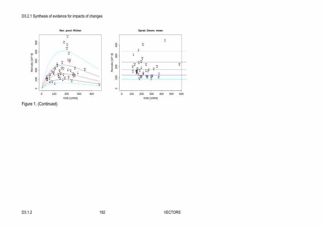
D3.2.1 Synthesis of evidence for impacts of changes  

D3.1.2 192 VECTORS

Figure 1. (Continued)

0 100 200 300 400 500 600

010

020

030

040

0

Sprat: Geom. mean

SSB [1000t]

Rec

ruits

[10

^-9]

6364656667 686970

71

72

80

81

82

83 8485

86

87

88

89

90

91

92

93

94

95

9697

98

99

0

1

23

4

56

7

8

9 10

11

0 100 200 300 400

010

020

030

040

050

0

Nor. pout: Ricker

SSB [1000t]

Rec

ruits

[10

^-9]

636465

66

67

68

69

707172

73

74

75

76

77

78

79

80

8182 83

8485

86

87

88

899091

92 93

94

95

96

97

98

99

01

2

34

56

7

8

9

10

11

D3.2.1 Synthesis of evidence for impacts of changes  

D3.1.2 193 VECTORS

Figure 2. Fitted relative stomach contents for Other Food as a function of year, quarter and predator length class. The relationship between observed and predicted relative stomach contents is shown in the lower right corner.

-0.4

0.0

0.4

part

ial f

or y

ear

year

81 85 87 91-0

.40.

00.

40.

8

part

ial f

or q

uart

er

quarter

1 2 3 4

250 300 350 400 450

-0.5

0.0

0.5

predml

part

ial f

or p

redm

l

0.2 0.4 0.6 0.8

0.5

0.7

x

y

                Year                                           Predator length l

              Quarter                                                 Observed

Predicted

Cod

D3.2.1 Synthesis of evidence for impacts of changes  

D3.1.2 194 VECTORS

Figure 2. (Continued)

-0.4

0.0

0.2

0.4

partia

l for

yea

r

year

81 85 87 91

-0.3

-0.1

0.1

0.3

partia

l for

qua

rter

quarter

1 2 3 4

200 250 300 350

-1.0

0.0

0.5

1.0

predmllo

(pre

dml)

0.1 0.3 0.5 0.7

0.1

0.3

0.5

x

y               Year                                                      Predator length class

              Quarter                                                            Observed

Predicted

Whiting

D3.2.1 Synthesis of evidence for impacts of changes  

D3.1.2 195 VECTORS

Figure 2. (Continued)

-1.5

-0.5

0.5

1.5

part

ial f

or y

ear

year

81 91

-2-1

01

23

part

ial f

or q

uart

er

quarter

1 2 3 4

-2.0

-1.0

0.0

1.0

part

ial f

or p

redm

l

predml

350 450 600

0.0 0.2 0.4 0.6 0.8 1.0

0.2

0.4

0.6

0.8

x

y

                Year                                           Predator length class

              Quarter                                                    Observed

Predicted

Saithe

D3.2.1 Synthesis of evidence for impacts of changes  

D3.1.2 196 VECTORS

Figure 3: Biomass indicator in Sub-area IV (number per hour for all length classes combined since the survey data are considered relevant for gurnards), based on IBTS-Q1. The plain line excludes the exceptional abundance observed occasionally in a single rectangle by shoal behavior (from ICES Advice in 2012).

D3.2.1 Synthesis of evidence for impacts of changes  

D3.1.2 197 VECTORS

Figure 4: Main predators of cod age 0 to age 2. The y axis shows the predation mortalities (M2).

D3.2.1 Synthesis of evidence for impacts of changes  

D3.1.2 198 VECTORS

Figure 5: Main predators of whiting age 0 to age 2. The y axis shows the predation mortalities (M2).

D3.2.1 Synthesis of evidence for impacts of changes  

D3.1.2 199 VECTORS

Figure 6. Estimated predation mortalities (M2) in the three hindcasts (run-81, run-91, keyrun).

Cod

Keyrun81 only91 only

1970 1980 1990 2000 2010

0.0

0.2

0.4

0.6

0.8

1.0

1.2

1.4

age 1

M2

1970 1980 1990 2000 2010

0.0

0.2

0.4

0.6

0.8

age 2

1970 1980 1990 2000 2010

0.00

0.10

0.20

0.30

age 3

D3.2.1 Synthesis of evidence for impacts of changes  

D3.1.2 200 VECTORS

Figure 7: Estimated predation mortalities (M2) in the three hindcasts (run-81, run-91, keyrun).

Whiting

Keyrun81 only91 only

1970 1980 1990 2000 2010

0.0

0.5

1.0

1.5

2.0

age 0

M2

1970 1980 1990 2000 2010

0.0

0.5

1.0

1.5

2.0

age 1

1970 1980 1990 2000 2010

0.0

0.2

0.4

0.6

0.8

1.0

age 2

D3.2.1 Synthesis of evidence for impacts of changes  

D3.1.2 201 VECTORS

Figure 8: Percentage of total mortality due to natural causes by species, year and age. Black line=age 0, red=age 1, green=age 2, blue=age 3.

1970 1980 1990 2000 2010

040

80

Cod

Per

cent

age

1970 1980 1990 2000 2010

040

80

Whiting

Per

cent

age

1970 1980 1990 2000 2010

040

80

Haddock

Per

cent

age

1970 1980 1990 2000 2010

040

80

Herring

Per

cent

age

1970 1980 1990 2000 2010

040

80

Sandeel

Per

cent

age

1970 1980 1990 2000 2010

040

80

Nor. pout

Per

cent

age

1970 1980 1990 2000 2010

040

80

Sprat

Per

cent

age

D3.2.1 Synthesis of evidence for impacts of changes  

D3.1.2 202 VECTORS

Figure 9: Predicted stock development of cod in the keyrun when all stocks are fished according to single species MSY related targets.

1990 1995 2000 2005 2010 2015 2020 2025

050

150

250

Cod SSB

SS

B (

1000

t)

1990 1995 2000 2005 2010 2015 2020 2025

0.0

0.2

0.4

0.6

0.8

1.0

Prob., SSB below 150 & 70

prob

abilit

y

1990 1995 2000 2005 2010 2015 2020 2025

0.0

0.2

0.4

0.6

0.8

1.0

Mean F

1990 1995 2000 2005 2010 2015 2020 2025

050

0010

000

1500

0 Recruits

Rec

ruits

(m

illion

s)

1990 1995 2000 2005 2010 2015 2020 2025

050

150

250

Eaten biomass

Eat

en b

iom

ass(

1000

t)

1990 1995 2000 2005 2010 2015 2020 2025

0.0

0.5

1.0

1.5

2.0

2.5

median M2 at age

M2

D3.2.1 Synthesis of evidence for impacts of changes  

D3.1.2 203 VECTORS

Figure 10: Predicted stock development of cod in run-81 when all stocks are fished according to single species MSY related targets.

1990 1995 2000 2005 2010 2015 2020 2025

050

100

200

Cod SSB

SS

B (

1000

t)

1990 1995 2000 2005 2010 2015 2020 2025

0.0

0.2

0.4

0.6

0.8

1.0

Prob., SSB below 150 & 70

prob

abilit

y

1990 1995 2000 2005 2010 2015 2020 2025

0.0

0.2

0.4

0.6

0.8

1.0

Mean F

1990 1995 2000 2005 2010 2015 2020 2025

010

0030

0050

00

Recruits

Rec

ruits

(m

illion

s)

1990 1995 2000 2005 2010 2015 2020 2025

050

100

150

Eaten biomass

Eat

en b

iom

ass(

1000

t)

1990 1995 2000 2005 2010 2015 2020 2025

0.0

0.5

1.0

1.5

2.0

median M2 at age

M2

D3.2.1 Synthesis of evidence for impacts of changes  

D3.1.2 204 VECTORS

Figure 11: Predicted stock development of cod in run-91 when all stocks are fished according to single species MSY related targets.

1990 1995 2000 2005 2010 2015 2020 2025

050

100

150

200

250

Cod SSB

SS

B (

1000

t)

1990 1995 2000 2005 2010 2015 2020 2025

0.0

0.2

0.4

0.6

0.8

1.0

Prob., SSB below 150 & 70

prob

abilit

y

1990 1995 2000 2005 2010 2015 2020 2025

0.0

0.2

0.4

0.6

0.8

1.0

Mean F

1990 1995 2000 2005 2010 2015 2020 2025

040

0080

0012

000

Recruits

Rec

ruits

(m

illion

s)

1990 1995 2000 2005 2010 2015 2020 2025

050

100

150

200

250

Eaten biomass

Eat

en b

iom

ass(

1000

t)

1990 1995 2000 2005 2010 2015 2020 2025

0.0

0.5

1.0

1.5

2.0

2.5

median M2 at age

M2

D3.2.1 Synthesis of evidence for impacts of changes  

D3.1.2 205 VECTORS

Figure 12: Predicted stock development of cod in run-gur when all stocks are fished according to single species MSY related targets.

1990 1995 2000 2005 2010 2015 2020 2025

010

020

030

0

Cod SSBS

SB

(10

00t)

1990 1995 2000 2005 2010 2015 2020 2025

0.0

0.2

0.4

0.6

0.8

1.0

Prob., SSB below 150 & 70

prob

abilit

y

1990 1995 2000 2005 2010 2015 2020 2025

0.0

0.2

0.4

0.6

0.8

1.0

Mean F

1990 1995 2000 2005 2010 2015 2020 2025

050

0010

000

1500

0 Recruits

Rec

ruits

(m

illion

s)

1990 1995 2000 2005 2010 2015 2020 2025

050

150

250

350

Eaten biomass

Eat

en b

iom

ass(

1000

t)

1990 1995 2000 2005 2010 2015 2020 2025

0.0

0.5

1.0

1.5

2.0

median M2 at age

M2

D3.2.1 Synthesis of evidence for impacts of changes  

D3.1.2 206 VECTORS

Figure 13: Predicted stock development of whiting in the keyrun when all stocks are fished according to single species MSY related targets.

1990 1995 2000 2005 2010 2015 2020 2025

010

030

050

0

Whiting SSB

SS

B (

1000

t)

1990 1995 2000 2005 2010 2015 2020 2025

0.0

0.2

0.4

0.6

Mean F

1990 1995 2000 2005 2010 2015 2020 2025

010

000

3000

050

000

Recruits

Rec

ruits

(m

illion

s)

1990 1995 2000 2005 2010 2015 2020 2025

020

040

060

080

0

Eaten biomass

Eat

en b

iom

ass(

1000

t)

1990 1995 2000 2005 2010 2015 2020 2025

0.0

0.5

1.0

1.5

2.0

median M2 at age

M2

D3.2.1 Synthesis of evidence for impacts of changes  

D3.1.2 207 VECTORS

Figure 14: Predicted stock development of whiting in run-81 when all stocks are fished according to single species MSY related targets.

1990 1995 2000 2005 2010 2015 2020 2025

010

020

030

040

050

0

Whiting SSB

SS

B (

1000

t)

1990 1995 2000 2005 2010 2015 2020 2025

0.0

0.2

0.4

0.6

Mean F

1990 1995 2000 2005 2010 2015 2020 2025

010

000

3000

0

Recruits

Rec

ruits

(m

illion

s)

1990 1995 2000 2005 2010 2015 2020 2025

010

030

050

0

Eaten biomass

Eat

en b

iom

ass(

1000

t)

1990 1995 2000 2005 2010 2015 2020 2025

0.0

0.5

1.0

1.5

2.0

2.5

median M2 at age

M2

D3.2.1 Synthesis of evidence for impacts of changes  

D3.1.2 208 VECTORS

Figure 15: Predicted stock development of whiting in run-89 when all stocks are fished according to single species MSY related targets.

1990 1995 2000 2005 2010 2015 2020 2025

010

030

050

0

Whiting SSB

SS

B (

1000

t)

1990 1995 2000 2005 2010 2015 2020 2025

0.0

0.2

0.4

0.6

Mean F

1990 1995 2000 2005 2010 2015 2020 2025

020

000

4000

060

000 Recruits

Rec

ruits

(m

illion

s)

1990 1995 2000 2005 2010 2015 2020 2025

020

040

060

080

0

Eaten biomass

Eat

en b

iom

ass(

1000

t)

1990 1995 2000 2005 2010 2015 2020 2025

0.0

0.5

1.0

1.5

2.0

2.5

median M2 at age

M2

D3.2.1 Synthesis of evidence for impacts of changes  

D3.1.2 209 VECTORS

Figure 16: Predicted stock development of whiting in run-gur when all stocks are fished according to single species MSY related targets.

1990 1995 2000 2005 2010 2015 2020 2025

010

030

050

0

Whiting SSB

SS

B (

1000

t)

1990 1995 2000 2005 2010 2015 2020 2025

0.0

0.2

0.4

0.6

Mean F

1990 1995 2000 2005 2010 2015 2020 2025

010

000

3000

050

000

Recruits

Rec

ruits

(m

illion

s)

1990 1995 2000 2005 2010 2015 2020 2025

020

040

060

080

0

Eaten biomass

Eat

en b

iom

ass(

1000

t)

1990 1995 2000 2005 2010 2015 2020 2025

0.0

0.5

1.0

1.5

2.0

median M2 at age

M2

D3.2.1 Synthesis of evidence for impacts of changes  

D3.1.2 210 VECTORS

Figure 17: Predicted stock development of whiting in the standard keyrun when all stocks are fished according to single species MSY related targets.

1990 1995 2000 2005 2010 2015 2020 2025

050

015

0025

00

Herring SSB

SS

B (

1000

t)

1990 1995 2000 2005 2010 2015 2020 2025

0.0

0.2

0.4

0.6

0.8

1.0

Prob., SSB below 1300 & 800

prob

abilit

y

1990 1995 2000 2005 2010 2015 2020 2025

0.0

0.1

0.2

0.3

0.4

0.5

Mean F

1990 1995 2000 2005 2010 2015 2020 2025

0e+0

04e

+04

8e+0

4

Recruits

Rec

ruits

(m

illion

s)

1990 1995 2000 2005 2010 2015 2020 2025

050

010

0015

00

Eaten biomass

Eat

en b

iom

ass(

1000

t)

1990 1995 2000 2005 2010 2015 2020 2025

0.0

0.2

0.4

0.6

0.8

1.0

median M2 at age

M2

D3.2.1 Synthesis of evidence for impacts of changes  

D3.1.2 211 VECTORS

Figure 18: Predicted stock development of herring in run-gur when all stocks are fished according to single species MSY related targets.

1990 1995 2000 2005 2010 2015 2020 2025

050

015

0025

00

Herring SSB

SS

B (

1000

t)

1990 1995 2000 2005 2010 2015 2020 2025

0.0

0.2

0.4

0.6

0.8

1.0

Prob., SSB below 1300 & 800

prob

abilit

y

1990 1995 2000 2005 2010 2015 2020 2025

0.0

0.1

0.2

0.3

0.4

0.5

Mean F

1990 1995 2000 2005 2010 2015 2020 2025

0e+0

04e

+04

8e+0

4

Recruits

Rec

ruits

(m

illion

s)

1990 1995 2000 2005 2010 2015 2020 2025

050

010

0015

00

Eaten biomass

Eat

en b

iom

ass(

1000

t)

1990 1995 2000 2005 2010 2015 2020 2025

0.0

0.2

0.4

0.6

0.8

1.0

median M2 at age

M2

D3.2.1 Synthesis of evidence for impacts of changes  

D3.1.2 212 VECTORS

Figure 19: Catch summed over the period from 2012 to 2025 as predicted with the keyrun when fishing cod at different target fishing mortalities and all other stocks according to MSY targets. Dotted lines indicate +/- one standard deviation, blue line the average value.

Figure 20: Catch summed over the period from 2012 to 2025 as predicted with run-81 when fishing cod at different target fishing mortalities and all other stocks according to MSY targets. Dotted lines indicate +/- one standard deviation, blue line the average value.

0

200000

400000

600000

800000

1000000

1200000

1400000

1600000

1800000

2000000

2200000

0.1 0.2 0.3 0.4 0.5 0.6 0.7 0.8

Catch in

 tonnes

Ftarget

0

200000

400000

600000

800000

1000000

1200000

1400000

1600000

1800000

2000000

0.1 0.2 0.3 0.4 0.5 0.6 0.7 0.8

Catch in

 tonnes

Ftarget

D3.2.1 Synthesis of evidence for impacts of changes  

D3.1.2 213 VECTORS

Figure 21: Catch summed over the period from 2012 to 2025 as predicted with run-91 when fishing cod at different target fishing mortalities and all other stocks according to MSY targets. Dotted lines indicate +/- one standard deviation, blue line the average value.

0

200000

400000

600000

800000

1000000

1200000

1400000

1600000

1800000

2000000

0.1 0.2 0.3 0.4 0.5 0.6 0.7 0.8

Catch in

 tonnes

F

D3.2.1 Synthesis of evidence for impacts of changes  

D3.1.2 214 VECTORS

Figure 22: Forecasted SSB trajectories in the keyrun dependent on the target fishing mortality for cod. Black line stands for a cod target F of 0.2, red lines for a F of 0.4 and blue lines for a F of 0.6.

1990 2000 2010 2020

0e+

002e

+05

4e+

056e

+05

17

Year

SS

B

1990 2000 2010 2020

0e+

004e

+05

8e+

05

18

Year

SS

B

1990 2000 2010 2020

0e+

004e

+05

8e+

05

19

Year

SS

B

1990 2000 2010 2020

010

0000

025

0000

0

21

Year

SS

B

Cod

Whiting

Haddock

Herring