marcus motshwane dept. of statistics university of limpopo pretoria-s.a
DESCRIPTION
Survival Analysis approach in evaluating the efficacy of ARV treatment in HIV patients at the Dr GM Hospital in Tshwane, GP of S. Africa. Marcus Motshwane Dept. of Statistics University of Limpopo Pretoria-S.A. Background. - PowerPoint PPT PresentationTRANSCRIPT

Survival Analysis approach in evaluating the efficacy of
ARV treatment in HIV patients at the Dr GM
Hospital in Tshwane, GP of S. Africa
Marcus Motshwane
Dept. of Statistics
University of Limpopo
Pretoria-S.A.

Background
• Survival analysis is aimed at estimating the probability of survival, relapse or death that occurs over time
• Relevant in clinical studies evaluating the efficacy of treatments in humans or animals
• Commonly deals with rates of mortality and morbidity
Problem statement
• The efficacy of ARV treatment at Dr G Mukhari hospital is favourable, but not clear as to the extend they are helpful to patients
• Survival analysis, a scientific statistical tool is conducted to-
-model ARV treatment efficacy in HIV patients
-confirm the association between
survival or not of patients after ARV treatment
Data Analysis
• 2007-2011 raw data
• 318 HIV/AIDS cases
• 24 variables selected
• STATA (12), SAS (9.2) & SPSS(21)

Year
2OO7 2OO8 2OO9 2O1O 2O110
5
10
15
20
25
30
16.04 15.72
20.44
27.67
20.13

No. of days on ARV
<180 181-360 361-540 541-720 721-900 901-1080 1081-1260
1261-1440
1441-1620
1621-1800
>18000
2
4
6
8
10
12
14
16
18
11.6
9.1
16.7
10.7
11.9
8.2
3.8
11
4.1
10.4
2.5

Age (Years)
15-25 26-35 36-45 46-55 56-65 66-750
5
10
15
20
25
30
35
40
8.2
36.8
30.8
18.6
5.3
0.3
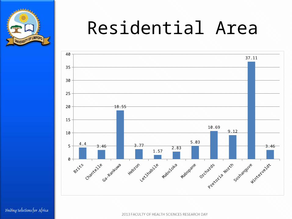
Residential Area
Brits
Chantel
le
Ga-Ran
kuwa
Hebro
n
Letlhab
ile
Maboloka
Mabopan
e
Orchard
s
Pretoria
North
Sosh
angu
ve
Winter
veldt
0
5
10
15
20
25
30
35
40
4.43.46
18.55
3.77
1.572.83
5.03
10.699.12
37.11
3.46

CD4 Count
0-100 101-200 201-300 301-400 401-500 501-600 601-7000
5
10
15
20
25
30
35
40
45
50
43.4
34.6
13.2
5
2.50.9 0.3

Viral Load
<1000 1001-50000 >500000
10
20
30
40
50
60
70
80
68.9
17.6
13.5

Survival function
• Used to describe the time-to-event concept for all patients.
• This is the probability of an individual to survive beyond time “x”and is defined as :
• Is a non-increasing function with a value of 1 at the origin and 0 at infinity.
• This is the case here with 1 at four days (4) and zero at the end of (1781) days, meaning that there is conformity with the survival function.

Kaplan-Meier Estimate
0.0
00
.25
0.5
00
.75
1.0
0
0 500 1000 1500 2000analysis time
Kaplan-Meier survival estimate

Kaplan-Meier estimate (cont)
• It is an estimator of the survival function- also called the product limit estimator
• It is a function of the probability of survival plotted against time
• In the ith interval, the probability of death can be estimated by:

Kaplan-Meier (cont)
• The estimated survival probability is:
= π
Where, - “d” = number of deaths observed at
time “t”
- “n”=the number of patients at risk
Kaplan-Meier (cont)
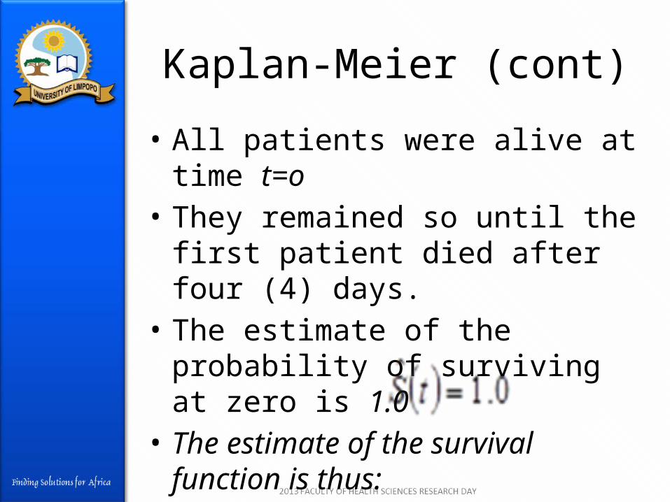
• All patients were alive at time t=o• They remained so until the first
patient died after four (4) days. • The estimate of the probability of
surviving at zero is 1.0• The estimate of the survival
function is thus:
at t=o

The log-rank test
Log-rank test for equality of survivor functions | Events Events group | observed expected ------+------------------------- 0 | 0 20.09 1 | 26 5.91 ------+------------------------- Total | 26 26.00 chi2(1) = 105.26 Pr>chi2 = 0.0000

The log-rank test (cont)
• The observed values are different from the expected values
• Produce a highly significant chi-squared value (P < 0.05).
• The null hypothesis is rejected at the 5% level of significance
• Survivor functions of the two groups are not the same.

Hazard function
0.0
005
.00
1.0
015
.00
2S
mo
othe
d ha
zard
fun
ctio
n
0 500 1000 1500analysis time
Cox proportional hazards regression

Hazard function
• It is the proportion of subjects dying or failing in an interval per unit of time
• As days pass, the number of patients dying also increases
• It is an increasing function as opposed to the non-increasing function of the Kaplan-Meier survival estimate.

Cox survival curve
0.2
.4.6
.81
Su
rviv
al
0 500 1000 1500 2000analysis time
Cox proportional hazards regression

Cox survival curve
• The graph of the estimated baseline survivor function
• The Cox approach is the most widely used regression model in survival analysis
• The probability of survival is 1 at time t=0
• Drops to “0” as the number of days elapses to maximum of 1781.

Cox regression model
No. of subjects = 312 Number of obs = 312 No. of failures = 26 Time at risk = 249675 LR chi2(7) = 13.54 Log likelihood = -96.694567 Prob > chi2 = 0.0599 ------------------------------------------------------------------------------ _t | Haz. Ratio Std. Err. z P>|z| [95% Conf. Interval] -------------+---------------------------------------------------------------- gender2 | .6791803 .2879292 -0.91 0.361 .2958897 1.558979 age | 1.032749 .0259595 1.28 0.200 .9831025 1.084903 marital2 | .3615232 .1486429 -2.47 0.013 .1614947 .8093083 education2 | 1.084283 .0966501 0.91 0.364 .9104767 1.291268 township2 | .8435348 .0977518 -1.47 0.142 .6721447 1.058628 cd4 | .9987908 .0023613 -0.51 0.609 .9941735 1.00343 viral | 1 5.54e-08 -0.20 0.845 .9999999 1 ------------------------------------------------------------------------------

Cox reg.model (cont)
• It asserts that the hazard rate for the ith subject in the data is
• The model is thus:

Cox reg.model (cont)
• Since P> 0.05 for gender, age, education, township, cd4 count and viral load,
• No significant statistical difference amongst these variables with regard to the predictor variable, days ARV.

Conclusion
• 92%(292/318) were alive after ARV treatment as compared to 8%(26/318) that died
• At the 5% level of significance, significant hazard ratios were characterised by hazard ratios that are significantly different from “1”, and 95% confidence interval (CI)
• ARV had a significant statistical impact on AIDS patients’ survival
• Overall mortality rates have decreased

IN MEMORY

Mrs Obama

FINALLY
THANK YOU