march 2, 2020 1 “what is socialism today? conceptions of a
TRANSCRIPT

March 2, 2020
“What is socialism today? Conceptions of a cooperative economy” 1 John E. Roemer* 2 Yale University 3
Abstract. Socialism is back on the political agenda in the United States. Politicians and some 6 economists who identify as socialists, however, do not discuss property relations, a topic that 7 was central in the intellectual history of socialism, but rather limit themselves to advocacy of 8 economic reforms, funded through taxation, that would tilt the income distribution in favor of the 9 disadvantaged in society. In the absence of a more precise discussion of property relations, the 10 presumption must be that ownership of firms would remain private or corporate with privately 11 owned shares. This formula is identified with the Nordic and other western European social 12 democracies. 13 In this article, I propose several variants of socialism, which are characterized by 14 different kinds of property relation in the ownership of society’s firms. In addition to varying 15 property relations, I include as part of socialism a conception of what it means for a socialist 16 society to possess a cooperative ethos, in place of the individualistic ethos of capitalist society. 17 Differences in ethea are modeled as differences in the manner in which economic agents 18 optimize. With an individualistic ethos, economic agents optimize in the manner of John Nash, 19 while under a cooperative ethos, they optimize in the manner of Immanuel Kant. It is shown 20 that Kantian optimization can decentralize resource allocation in ways that neatly separate issues 21 of income distribution from those of efficiency. In particular, remuneration of labor and capital 22 contributions to production need no longer be linked to marginal-product pricing of these factors, 23 as is the key to efficiency with capitalist property relations. I present simulations of socialist 24 income distributions, and offer some tentative conclusions concerning how we should conceive 25 of socialism today. 26 27
28
Key words: market socialism, general equilibrium, cooperation, Kantian optimization, first 29
theorem of welfare economics 30
JEL codes: D3, D6, P2, P5, H4 31
32 33 34 35 36 37
* I am grateful to Joaquim Silvestre for many discussions and advice. I thank as well Fred Block, Mordecai Kurz, and Gabriel Zucman for advice on data. I received useful valuable written comments from Philippe De Donder, Suresh Naidu and Roberto Veneziani. Attendees at seminar presentations at Yale, Dalhousie University, the Columbia University Political Economy Conference, the Université Catholique de Louvain and the September Group also provided important feedback. All remaining errors are my own.
1
1. Introduction 1 2
Socialism is back on the political agenda in the United States. Bernie Sanders and 3
Alexandria Ocasio-Cortez (AOC) are self-declared socialists, and the Democratic Socialists of 4
America has grown exponentially in the last few years. Most of the current crop of Democratic 5
Party would-be presidential candidates support policies that many call socialist – single-payer 6
health insurance, guaranteed employment, massive infrastructural investment, universal pre-7
school, and state-financed tertiary education. About one-half of young adults in the United 8
States polled in surveys state they prefer socialism to capitalism1. 9
At least five recent books discuss the ills of capitalism, and recommend reforms: Piketty 10
(2015), Atkinson (2015), Corneo (2017), Stiglitz (2019) and Saez and Zucman (2019). Piketty 11
argues that the period of the trente glorieuses , 1945-1975, when income inequality in the 12
advanced capitalist democracies was low by historical standards and the welfare state was 13
ascendant, was not an advanced phase of a more benign capitalism, but rather a pause in the 14
otherwise steady increase in the concentration of wealth and income, brought about by the 15
catastrophes of the 20th century – two world wars and a depression—that set capital on its heels. 16
His central reform proposal is to tax wealth. Atkinson and Stiglitz propose menus of reform to 17
weaken capital and increase the real income of the working and middle classes – the latter would 18
be funded in the main by taxation—as well as anti-trust and pro-labor legislation that would alter 19
the bargaining power of labor and capital in labor’s favor. Corneo proposes that the state 20
purchase shares of capitalist corporations, eventually taking a sizable share of corporate profits 21
for the public purse. Saez and Zucman are concerned with raising substantially taxes on the very 22
rich. The reforms proposed by Sanders, AOC, Piketty, Atkinson, Corneo ,Stiglitz , and Saez 23
and Zucman would implement a kind of socialism called social democracy, whose defining 24
characteristic is that capitalist property relations – centrally, the private ownership of firms—25
would remain largely intact, as would the income allocation rule. Investment in infrastructure, 26
research, and human beings would increase substantially, funded by taxation. Stiglitz, indeed, 27
calls his design ‘progressive capitalism,’ rather than social democracy. The most advanced 28
1 The GenForward Survey, conducted by the University of Chicago, whose respondents are between the ages of 18 and 34, reports that 49% hold a favorable view of capitalism and 45% hold a favorable view of socialism. Sixty-two percent think ‘we need a strong government to handle today’s complex economic problems.’ (Chicago Tribune, May 18, 2018)

2
examples of social democracy in today’s world are the economic regimes in the Nordic countries 1
– as one travels south in Europe, social democracy becomes somewhat attenuated, although in 2
France, the state still collects approximately one-half of the national income in taxes. Social 3
democracy has become attenuated over time, as well as space, in Europe, as in almost all 4
countries, the state’s share of national income has fallen in the last twenty years. 5
Social democracy, however, is only one variant of socialism. At the other pole on the 6
interval of socialist variants is the regime of central planning, best represented by the Soviet 7
Union and China prior to 1979. It is fair to say that the architects of the centrally planned 8
economies were attempting to implement what they saw as Karl Marx’s vision of socialism, a 9
system in which private ownership of firms (the ‘means of production’) is abolished and replaced 10
by state ownership. Combining state ownership with central planning (in place of market 11
allocation) and political control by one party (in place of democracy) turned out to deliver a toxic 12
cocktail, from both the political and economic viewpoints. While central planning in the Soviet 13
Union engendered rapid industrialization, and in particular enabled the Russians to turn around 14
Hitler’s onslaught to the east, economic development eventually atrophied after the low-hanging 15
fruit had been gathered – moving large populations of semi-employed peasants into urban 16
industry (see Allen [2003]). The absence of democratic political competition, in combination 17
with the absence of decentralization via markets, induced economic atrophy. The Chinese, 18
however, through the introduction of markets and quasi-private property in rural areas, beginning 19
in 1979, developed a dual economy, with a fast-growing private sector, and a slow-growing but 20
still significant state sector. 21
My intention in this paper is to retrieve, from the history of the socialist idea, several 22
alternatives to these two socialist varieties. I set the stage by noting that any socio-economic 23
system has (in my view) three pillars: an ethos of economic behavior, an ethic of distributive 24
justice, and a set of property relations that will implement the ethic if the behavioral ethos is 25
followed. Our understanding of these three pillars evolves as history unfolds. The behavioral ethos 26 of socialism is cooperation. Citizens of a socialist society should recognize that they are engaged in 27
a cooperative enterprise to transform nature in order to improve the lives of all. The distributive 28 ethic, classically, is ‘from each according to his ability, to each according to his work.’ In the last 29
fifty years, some writers have replaced this formula with one of pervasive equality of opportunity. 30
The philosopher John Rawls argued that persons do not deserve to benefit or suffer by dint of the 31

3
resources they are assigned in the ‘birth lottery.’ In the light of the discussion initiated by Rawls, 1
G.A. Cohen has argued that the distributive ethic of socialism should now be taken to be ‘socialist 2 equality of opportunity,’ which he defines as follows: 3
Socialist equality of opportunity seeks to correct for all unchosen disadvantages, disadvantages, that is, for 4 which the agent cannot herself reasonably be held responsible, whether they be disadvantages that reflect 5 social misfortune or disadvantages that reflect natural misfortune. When socialist equality of opportunity 6 prevails, differences of outcome reflect nothing but differences of taste and choice, not differences in natural 7 and social capacities and powers (Cohen [2009, p.5])2. 8
The property relations of socialism are meant to implement socialist equality of opportunity, 9
so far as this is possible in a market economy, and to reflect the cooperative ethos of economic 10
behavior. Large firms (although not small ones) will not have owners to whom profits accrue – 11
rather, the entire income of firms will be distributed to those who contribute inputs of production – of 12 labor and capital. 13
I contrast these socialist pillars with the analogous pillars of capitalism. Capitalism’s 14
behavioral ethos is individualistic: economic activity is characterized as the struggle of each person 15
against all other persons and nature. The ethos may be summarized as one of ‘going it alone.’ The 16 distributive ethic of capitalism is laissez-faire: it is right and admirable for individuals to materially 17
prosper without bound, as long as they do not interfere with the opportunity of others to so prosper: 18
‘from each according to his endowments, to each what he can get.’ Children may rightly gain by 19 virtue of everything they receive in the birth lottery, and others may duly suffer by bad luck in that 20
lottery. Freedom of contract is paramount, even if its consequences are to impede equality of 21
opportunity, as inheritance of vast wealth surely does. Property relations in firms are private: 22 individuals own firms, and their profits accrue to the owners after the costs of production are met, 23
including the payment of wages to labor and rent or interest to investors. 24
In this article, I focus on the behavioral ethos and property relations of socialism. ( I have 25
presented my views on socialism’s distributive ethic in Roemer (2017).) I will propose how to 26
model cooperation, and embed that model in general-equilibrium models that feature several 27
variants of what socialist property relations might be. The first variant of socialism that I 28
propose is a version of social democracy, amended to include the cooperative behavioral ethos. 29
Call this Socialism 1. A second variant, Socialism 2, I call a sharing economy; its distributive 30
2 Cohen (2009) defines three levels of equal opportunity, which he calls bourgeois, left-liberal and socialist.

4
ethic is ‘from each according to his ability, to each according to his contribution,’ a variant on 1
Marx’s famous dictum. These two variants of socialism share with capitalism two features: 2
markets exist for capital, labor and commodities, and firms maximize profits. 3
Socialism 2 differs from capitalism and Socialism 1 in that firm profits are not distributed 4
to shareholders, but only to those who contribute inputs to the firm, of labor and capital. The 5
background model of capitalism is the Arrow-Debreu model, in which a distinction is made 6
between shareholders, who hold a property right in the surplus accruing to the firm after factor 7
payments to labor and capital have been made, and investors who supply capital to the firm. I 8
will review a simple version of this model in section 2 below. 9
While the usual distinction emphasized between capitalism and socialism concerns their 10
property relations, I wish here to place equal focus on their different behavioral ethea: the 11
individualistic ethos of capitalism versus the cooperative ethos of socialism. I have said the 12
former pictures the economic struggle as one of each person against all other persons and nature, 13
while the latter conceptualizes that struggle as one of people in cooperation against nature. I 14
propose that the individualistic ethos is modeled ( in game theory) by Nash optimization, in 15
which each individual treats the actions of other persons as parametric. Similarly, the 16
cooperative ethos (in game theory) is modeled as Kantian optimization, where each individual 17
contemplates what can be achieved if all take similar actions in concert. 18
That capitalism is based upon an individualistic behavioral ethos has been recognized for 19
centuries, for which one need only consult Adam Smith’s famous adage about what motivates 20
small businessmen. Smith, of course, argued that the individualistic ethos would result, given 21
certain rules and a market economy, in an outcome that was good for the many, an idea that is 22
represented today in the first theorem of welfare economics. Likewise, it has been a long-23
established view that socialism assumes or requires that people cooperate in their economic 24
activity. Models of socialist economies, however, have as yet not incorporated cooperative 25
behavior, except to the extent that one might, tautologically, consider non-capitalist property 26
relations in firms to constitute a form of cooperation. I say that non-capitalist property relations 27
alone are insufficient to characterize the cooperative ethos. If we include a precise behavioral 28
model of cooperation as a necessary component of socialism, we can extend Smith’s adage, as 29
will be shown – stronger forms of the first theorem of welfare economics will obtain under 30
socialism. 31
5
In sum, my task here is expand the conception of socialism as a regime of economic 1
allocation beyond the version that is dominating the current political discussion, the version of 2
social democracy. I will then propose another socialist variant that represents an older idea, that 3
socialism requires new property relations in firms. Non-private-ownership in these variants, 4
however, is not to be identified with bureaucratic control by the state of the firms’ actions. Firms 5
will in all cases maximize profits in a market economy, but the distribution of firms’ income will 6
neither be according to the rules of capitalism nor bureaucratic diktat, but according to specific 7
rules that are defined for the variant in question. I will be concerned with the efficiency 8
properties of these socialist variants--to be precise, what form, if any, the first theorem of welfare 9
economics takes. Just the way Pareto efficiency in a capitalist economy depends upon profit 10
maximization and Nash optimization, so in my socialist variants, it depends upon profit 11
maximization and Kantian optimization. As important in varying the property relations 12
governing firms from capitalist ones, so I claim, is the incorporation of a formal model of 13
cooperation in economic behavior. 14
The conclusion is that we can substitute non-capitalist property relations for laissez-faire 15
capitalist ones, and preserve and extend the result that equilibria are decentralizable and Pareto 16
efficient, even in the presence of redistributive taxation, public bads, and public goods. These 17
results suggest that we should cease viewing Nash optimization as the universal conception of 18
rational behavior in games, but think of it rather as representing the individualistic ethos that is 19
part and parcel of capitalism. What are typically called market failures are reinterpreted as 20
failures – rather – of Nash optimization. 21
Finally, I will offer some thoughts regarding what variant of socialism is most 22
appropriate today. 23
24
2. The capitalist economy (Arrow-Debreu) 25
26
Let’s begin with a simple economy in which a good is produced from labor and capital. 27
There is a firm with a production function , whose arguments are capital (K) and 28
labor ( L), measured in efficiency units. We assume that G is increasing, differentiable, and 29
concave. A private firm owns the technology G. The population consists of n individuals; the 30
preferences of individual i are represented by a quasi-concave differentiable utility function 31
G :ℜ+2 →ℜ+
6
, defined on vectors of the consumption good, labor, and capital, where utility 1
is increasing in consumption and decreasing in labor and capital supplied. Individual i possesses 2
an endowment of capital and (efficiency units of) labor . Individual i also owns a share 3
of the firm. This market economy will display prices, for the consumption good (p), labor 4
(w), and capital (r ). We do not explain how capital was produced: it is simply an endowment of 5
individuals, coming from the un-modeled past. 6
7
Definition 1. A competitive equilibrium for the economic environment 8
comprises a price vector , demands for capital and labor 9
by the firm , a supply of the good by the firm, demands for the good by 10
the n consumers, supplies of labor and capital by the consumer-worker-11
investors such that: 12
• maximizes , subject to ; we denote profits by 13
; 14
• maximizes subject to 15
16
• Markets clear: 3 17
18
The first-order conditions for profit-maximization by the firm are: 19
(2.1) 20
3 Equivalently, one could define preferences on the three goods of consumption, leisure and capital services (what capital the agent does not invest). I define preferences as including a desire for capital services (e.g., security) in order to treat labor and capital symmetrically. We could assume that the agents place no value on retained capital, so that capital is inelastically supplied in its entirety to firms; however, that asymmetry would complicate the presentation below because we would have constantly to pay attention to corner solutions.
ui (⋅,⋅,⋅) (x,L,K )
Ki Li
θi
{G,{ui ,Ki ,Li ,θi | i = 1,...,n}} (p,w,r)
(K *,L*) y* (x1,..., xn )
(L1,...,Ln ) (K1,...,Kn )
(y*,K *,L*) py − rK −wK y = G(K ,L)
Π* = py* − rK * −wL*
(xi ,Li ,Ki ) ui (x,L,K )
px = wL+ rK + θiΠ*
Li ≤ Li
K i ≤ K i
y* = xi , L* = Li , and K * = Ki .∑∑∑
G1(K ,L) = rp
and G2 (K ,L) = wp
,

7
where is the jth partial derivative of G, for At equilibrium, it makes sense to say 1
that worker i’s contribution to production is , if is small compared to , since 2
if i withdraws her labor, the product falls by approximately this amount. Likewise, the 3
(approximate) contribution of investor i’s capital to production is . Thus the total 4
contribution of the factor owners to production is: 5
(2.2) 6
where the strict inequality holds if G is strictly concave. That is, after the factor owners are paid 7
for their contributions, a surplus remains, which is the firm’s profit. 8
The average product of the firm is: 9
; (2.3) 10
this is output per unit of input contribution. Because the average product is greater than unity for 11
a strictly concave production function, production in general yields a surplus – output is greater 12
than the sum of factor contributions. 13
Often, neoclassical economists say that profits are not a surplus, but a return to 14
entrepreneurial or managerial talent. But this is a just-so story. Entrepreneurial talent does not 15
exist in this model. If it did, we should write the production function as , where M is 16
entrepreneurial labor. If m were the wage of such labor, then the firm would maximize profits 17
by maximizing: 18
. (2.4) 19
If the entrepreneurial input were really the missing input that explains profits, then it must be that 20
at the solution to (2.4), profits are zero: that is, we would have 21
, (2.5) 22
where is the jth partial derivative of , and I have used the fact that each factor is paid its 23
marginal value product at the profit-maximizing solution. Now dividing (2.5) by p gives us: 24
, (2.6) 25
and so profits are zero if the function is homogeneous of degree one. 26
Gj j = 1,2.
wpLi Li LS ≡ Li∑
rpK i
G1(K*,L*)K * +G2 (K
*,L*)L* <G(K *,L*),
G(K *,L*)G1(K
*,L*)K * +G2 (K*,L*)L*
G(M ,K ,L)
pG(M ,K ,L)−mM −wL − rK
pG(M *,K *,L*) = mM * + rK * +wL* = (pG1)M* + (pG2 )K
* + (pG3)L*
G j G
G(M *,K *,L*) = G1 ⋅M* + G2 ⋅K
* + G3 ⋅L*
G
8
However, as I said, it is a fiction to claim that profits are a return to entrepreneurial 1
labor4. Certainly, in the modern corporation, managers are paid salaries (wages), and if the 2
firm is viable, profits are positive after those salaries are paid. And there is no market for 3
entrepreneurial labor, although metaphorically, one might think of venture capitalists as 4
attempting to create one. 5
It is certainly commonplace in economics to argue that viewing production functions as 6
characterized by decreasing returns is myopic, in the sense that McKenzie (1959) and others 7
argue. My claim is that this view is a tautology, and should not be used to justify profits as a de 8
facto payment for an invisible input. Surely, one can contract concerning property rights to the 9
firm’s profits, or the firm’s value, but it would be mystical to write contracts concerning the 10
ownership of an invisible production factor. Viewing profits as a return to an invisible factor is 11
an ‘as if’ statement, which, if believed, limits our ability to conceptualize non-capitalist property 12
relations in firms. 13
There are three remarks: 14
(A1) As is well-known, the competitive equilibrium is Pareto efficient, a fact known as 15
the first theorem of welfare economics; 16
(A2) The price system decentralizes the competitive allocation, in the sense that: 17
o The firm need only know prices and its production function G, but not the 18
preferences of consumers; 19
4 In their classic article, Arrow and Debreu (1954, p. 267) write, “The existence of factors private to the firm is the standard justification in economic theory for decreasing returns to scale.” They in turn cite similar statements in earlier papers by Hicks and Samuelson. This view, however, conflicts with the postulate that commodities are goods (including labor) that trade on markets. Surely managerial labor is a commodity; it commands a salary. The entrepreneurial input, on the other hand, typically does not trade on markets, and it is only a metaphor to say that profits equal the value of the entrepreneurial input. It is an ethically loaded metaphor that disguises the more concrete view that profits are the surplus that remains after factor inputs are paid for, which redound to the residual claimant. Perhaps the most militant defender of the claim that neoclassical profits in a decreasing-returns world are in fact the return to an unstated entrepreneurial input is McKenzie (1959, p. 66). Indeed, in is general-equilibrium work, McKenzie derives the case of decreasing returns as a corollary to the case of constant returns, where an ‘entrepreneurial factor’ is fixed. He writes, “To bring this model [i.e., decreasing returns] within the linear model we have described, we must introduce the entrepreneurial factor which is private to the firm and not marketed (my italics, JER).”

9
o Consumers need only know prices, their preferences, and their profit 1
remittances from firms. 2
3
It is these attributes that summarize the main virtues of the capitalist system, viewed as a 4
resource-allocation device. To be somewhat more circumspect, the dynamic efficiency of 5
capitalism – its tendency to foster innovation and productivity increases -- is not modeled here. 6
The Pareto efficiency of the equilibrium is a stand–in for that important aspect of capitalism. 7
The informal view is that profit-maximization induces innovation and technological advance, as 8
capitalists seek to survive in competitive markets. 9
To these, I add a third remark: 10
(A3) Workers and investors receive precisely their contributions to production, while the 11
firm owners receive the entire surplus. The fairness of this allocation is questionable. For is it 12
not arguable that workers and investors should share in the surplus that emerges in production? 13
The legal structure of capitalism allocates profits to owners, but that is not necessarily fair or 14
ethical. It is a tradition in neoclassical theory to say that workers are not exploited if they 15
receive wages equal to their marginal (value) products. Marxists, however, say that workers 16
who receive marginal-product wages are exploited because they do not share in the surplus from 17
production. In our present model, investors should probably also be viewed as exploited (by 18
Marxists) for they, too, receive only their contributions to production and do not share in the 19
surplus.5 20
The model of this section is too sparse to enable us to conclude definitively whether 21
workers and investors are exploited, or unfairly treated, for it does not report the history whereby 22
individuals became owners, workers, and/or investors of the firm. Therefore, I will not press the 23
case here that workers and investors are exploited, but will be satisfied with the more benign 24
statement that they are paid precisely their contributions to production, and do not share in the 25
surplus produced, which legally is distributed to the firm’s owners. 26
5 Marx argued that capital did not come about, in its original form, from honest labor, and so he would have laughed at the thought that those who provide capital to the firm should be considered exploited. But if some capital accumulation does emerge through honest activity (such as savings from labor income), it might well be appropriate for a Marxist to consider those who provide capital to a firm exploited, if they are paid precisely their contribution to production and do not share in the economic surplus.
10
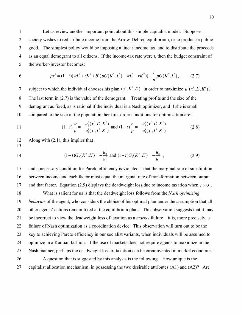
Let us review another important point about this simple capitalist model. Suppose 1
society wishes to redistribute income from the Arrow-Debreu equilibrium, or to produce a public 2
good. The simplest policy would be imposing a linear income tax, and to distribute the proceeds 3
as an equal demogrant to all citizens. If the income-tax rate were t, then the budget constraint of 4
the worker-investor becomes: 5
, (2.7) 6
subject to which the individual chooses his plan in order to maximize . 7
The last term in (2.7) is the value of the demogrant. Treating profits and the size of the 8
demogrant as fixed, as is rational if the individual is a Nash optimizer, and if she is small 9
compared to the size of the population, her first-order conditions for optimization are: 10
(2.8) 11
Along with (2.1), this implies that : 12 13
, (2.9) 14
and a necessary condition for Pareto efficiency is violated – that the marginal rate of substitution 15
between income and each factor must equal the marginal rate of transformation between output 16
and that factor. Equation (2.9) displays the deadweight loss due to income taxation when . 17
What is salient for us is that the deadweight loss follows from the Nash optimizing 18
behavior of the agent, who considers the choice of his optimal plan under the assumption that all 19
other agents’ actions remain fixed at the equilibrium plans. This observation suggests that it may 20
be incorrect to view the deadweight loss of taxation as a market failure – it is, more precisely, a 21
failure of Nash optimization as a coordination device. This observation will turn out to be the 22
key to achieving Pareto efficiency in our socialist variants, when individuals will be assumed to 23
optimize in a Kantian fashion. If the use of markets does not require agents to maximize in the 24
Nash manner, perhaps the deadweight loss of taxation can be circumvented in market economies. 25
A question that is suggested by this analysis is the following. How unique is the 26
capitalist allocation mechanism, in possessing the two desirable attributes (A1) and (A2)? Are 27
pxi = (1− t)(wLi + rK i +θ i (pG(K *,L*)−wL* − rK *))+ tnpG(K *,L*)
(xi ,Ki ,Li ) ui (xi ,Li ,Ki )
(1− t)wp= − u2
i (xi ,Li ,Ki )u1i (xi ,Li ,Ki )
and (1− t) rp= − u3
i (xi ,Li ,Ki )u1i (xi ,Li ,Ki )
(1− t)G2 (K *,L*) = − u2i
u1i and (1− t)G1(K
*,L*) = − u3i
u1i
t > 0

11
the Pareto efficiency of equilibrium and the decentralization of resource allocation necessarily 1
associated with marginal-product remuneration of factors, and private ownership of firms? 2
3
3. Kantian optimization: Modeling cooperation6 4
Let be a game in normal form with n players, where the payoff functions 5
and I is an interval in , the strategy space for each player. We call the 6
strategies ‘contributions’ or ‘efforts.’ A game is strictly monotone increasing 7
(decreasing) if each payoff function is a strictly increasing (decreasing) function of the 8
contributions of the players other than i. 9
Definition 2 10
a) A constant strategy profile is a simple Kantian equilibrium if: 11
; (3.1) 12
b) A strategy profile is an additive Kantian equilibrium if: 13
; (3.2) 14
c) A strategy profile is a multiplicative Kantian equilibrium if 15 . (3.3) 16
The appellation ‘Kantian’ is derived from the ‘simple’ case: here, E is the contribution 17
that each player would like all players to make. In Immanuel Kant’s language, each player is 18
taking the action he ‘would will be universalized.’ 19
In an additive Kantian equilibrium, no player would desire to translate the strategy 20
profile by any constant vector. In a multiplicative Kantian equilibrium, no player would desire 21
to re-scale the strategy profile by any factor. 22
23
Remark. The concepts of additive and multiplicative Kantian equilibrium nest simple Kantian 24
equilibrium. Any simple Kantian equilibrium is an additive and multiplicative Kantian 25
equilibrium. 26
6 This section reviews material discussed thoroughly in Roemer (2019).
V = (V 1,...,V n )
V i : I n →ℜ ℜ+
Ei ∈I
V i
(E,E,...,E)
(∀i)(E = argmaxx∈I
V i (x, x,..., x))
(E1,...,En )
(∀i)(0 = argmaxρ
V i (E1 + ρ,E2 + ρ,...,En + ρ))
(E1,...,En )(∀i)(1= argmax
ρV i (ρE1,ρE2,...,ρEn ))

12
If the game V is symmetric (for example, there is a function such that for all i, 1
where ) then a simple Kantian equilibrium exists. For 2
games with heterogeneous payoff functions, simple Kantian equilibria generally do not exist, but 3
additive and multiplicative Kantian equilibria often do. 4
The important fact is: 5
6
Proposition 1. In any strictly monotone game, simple and additive Kantian equilibria are 7
Pareto efficient, and any strictly positive multiplicative Kantian equilibrium is Pareto efficient. 8
Proof: Roemer (2019). 9
10
Strictly increasing games are games with positive externalities, where contributions 11
create a public good. Strictly decreasing games are games with negative externalities – games 12
with congestion effects. Proposition 1 justifies calling Kantian optimization a protocol of 13
‘cooperation’, for it resolves efficiently the free rider problem (in monotone increasing games) 14
and the tragedy of the commons (in monotone decreasing games) that characterize Nash 15
optimization in the presence of externalities. 16
In what follows, we embed Kantian optimization of various kinds in simple general-17
equilibrium models of socialism. 18
19
4. Socialism 1: Social democracy 20
As defined in section 1, social democracy is an economic mechanism in which firms 21
remain privately owned, individuals contribute factor inputs to firms, but taxation redistributes 22
incomes, perhaps substantially. In this section, we show that social democracy, conceived as a 23
mechanism where citizens optimize according to a Kantian protocol, separates the issue of 24
income distribution from that of efficiency. Pareto efficient allocations are achievable with any 25
degree of income taxation. 26
We first define two games for the economic environment . 27
The workers’ game is given by the payoff functions , which are defined on the vector of 28
labor supplies: 29
30
V
V i (E1,...,En ) = V (Ei ,ES\i ), ES\i = E j
j≠i∑
{G,{ui ,Ki ,Li ,θi | i = 1,...,n}}
W i

13
, (4.1) 1
where for any variable z, and . The term 2
is the amount of the consumption good that can be purchased with the 3
demogrant from taxation that is returned to each individual. Note that workers and investors 4
treat profits parametrically, but take into account the effect of their contributions on the 5
demogrant. 6
The investors’ game is given by the same payoff functions, but defined on the vector of 7
capital investments: 8
. (4.2) 9
The payoff functions are ‘identical’ in these two games, but the strategy spaces on 10
which they are defined differ. In the workers’ game, the parameters are 11
, while in the investors’ game, the parameters are 12
. 13
To clarify, each person is (in general) both a worker and an investor. She will participate 14
as a player in both of the above games, where in one her strategy is a supply of labor, and in the 15
other her strategy is a supply of capital. 16
17
Definition 3. A social democratic (Socialist 1) equilibrium for the economic environment 18
at tax rate t, comprises a price vector , demands for labor 19
and capital by the firm , a supply of the good by the firm, demands for the good 20
by the n agents, supplies of labor and capital by the worker-21
investors such that: 22
• maximizes , subject to we denote profits by 23
; 24
W i(L1,L2 ,...,Ln ) = ui((1− t)(wLi + rK i + θiΠ(K *,L*))
p+ tnwLS + rK S +Π(K *,L*)
p,Li ,K i )
zS = zi∑ Π(K *,L*) = pG(K *,L*)−wL* − rK *
tnwLS + rK S +Π(K *,L*)
p
V i (K1,K 2,...,Kn ) = ui ((1− t)(wLi + rK i + θiΠ(K *,L*))
p+ tnwLS + rK S +Π(K *,L*)
p,Li ,Ki )
W i and V i
(p,w,r,K1,...,Kn ,K *,L*)
(p,w,r,L1,...,Ln ,K *,L*)
{G,{ui ,Ki ,Li ,θi | i = 1,...,n}} (p,w,r)
(K *,L*) y*
(x1,..., xn ) (L1,...,Ln ) (K1,...,Kn )
(y*,K *,L*) py − rK −wL y = G(K ,L);
Π* = pG(K *,L*)− rK * −wL*

14
• The vector is an additive Kantian equilibrium of the workers’ game 1
, given ; 2
• The vector is an additive Kantian equilibrium of the investors’ game 3
, given ; 4
• For all i, 5
• All markets clear: . 6
7
The tax rate t is exogenous. Clearly, what differentiates social-democratic equilibrium from 8
capitalist equilibrium is that workers and investors choose their contributions in a cooperative 9
manner, according to the additive Kantian protocol. The consequence of using this protocol is: 10
11
Proposition 2 Let be the allocation at a social-democratic equilibrium at 12
any tax rate . The equilibrium is Pareto efficient. 13
Proof: 14
1. By profit-maximization, 15
2. I state what it means for to be an additive Kantian equilibrium of the game W, 16
given 17
18
19
Calculate that this reduces to: 20
. 21
But this says: 22
23
(L1,...,Ln )
W = {W i} (K1,...,Kn )
(K1,...,Kn )
V = {V i} (L1,...,Ln )
xi = (1− t)(wLi + rK i + θiΠ(K *,L*))
p+ tnG(KS ,LS );
xS = y*,LS = L*,KS = K *
(K *,L*, y*,{Ki ,Li , xi})
t ∈[0,1]
pG1(K*,L*) = r and pG2 (K *,L*) = w.
(L1,...,Ln )
(K1,...,Kn ) :
(∀i) ddρ ρ=0
ui (1− t)(w(Li + ρ)+ rK i + θiΠ(K *,L*))
p+ tnw(LS + nρ)+ rK S +Π(K *,L*)
p,Li + ρ,Ki⎛
⎝⎜⎞⎠⎟= 0.
(∀i)u1i ⋅ (1− t)w
p+ tnwnp
⎛⎝⎜
⎞⎠⎟+ u2
i = 0
(∀i)(wp= − u2
i
u1i ).
15
3. In like manner, the condition that be an additive Kantian equilibrium of the game 1
V given is, for all i, . 2
4. From steps 1, 2, and 3, we have: 3
. 4
Given concavity, these are precisely the conditions that the equilibrium allocation be Pareto 5
efficient. ■ 6
7
The key to this ‘first theorem of welfare economics’ in social democracy can be seen by 8
comparing the proof of Proposition 2, to equations (2.8) and (2.9), which are the first-order 9
conditions of optimality for a Nash optimizing factor owner. The ‘wedge’ that renders 10
unequal the marginal rate of transformation and the consumer’s marginal rates of substitution in 11
these equations appears because the Nash optimizer’s counterfactual is that only he alters his 12
factor supply, while others’ factor supplies remain fixed. The additive Kantian optimizer’s 13
counterfactual, in contrast, is that the entire vector of labor supplies is translated by a common 14
constant. It then turns out that the reduction of the wage through taxation is exactly 15
compensated for by the addition to income from the demogrant, and there is no wedge between 16
the marginal rate of transformation and the consumer’s marginal rate of substitution. 17
We have: 18
Proposition 3. Let G be strictly concave and satisfy the Inada conditions. Let preferences be 19
convex. Then, for any , a social-democratic equilibrium exists. 20
Proof: Appendix. 21
22
Five remarks are in order. The first concerns the information the optimizing agent (say, 23
the worker) needs to compute her optimal labor supply in equilibrium. Under Nash optimization, 24
she needs to know prices and the tax rate. The Kantian optimizing worker needs to know only 25
prices. She need not know the tax rate, because with additive Kantian optimization, if she 26
(K1,...,Kn )
(L1,...,Ln ) rp= − u3
i
u1i
(∀i) G1(K*,L*) = − u3
i
u1i and G2 (K *,L*) = − u2
i
u1i
⎛⎝⎜
⎞⎠⎟
(1− t)
t ∈[0,1]
16
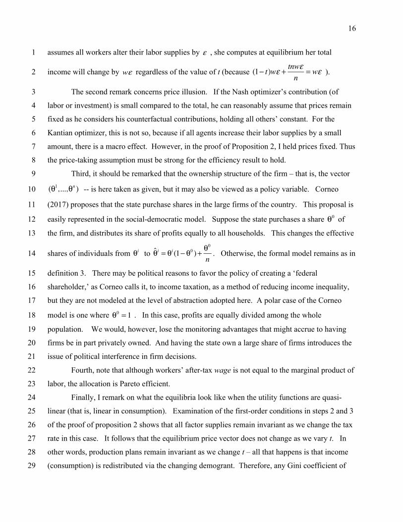
assumes all workers alter their labor supplies by , she computes at equilibrium her total 1
income will change by regardless of the value of t (because ). 2
The second remark concerns price illusion. If the Nash optimizer’s contribution (of 3
labor or investment) is small compared to the total, he can reasonably assume that prices remain 4
fixed as he considers his counterfactual contributions, holding all others’ constant. For the 5
Kantian optimizer, this is not so, because if all agents increase their labor supplies by a small 6
amount, there is a macro effect. However, in the proof of Proposition 2, I held prices fixed. Thus 7
the price-taking assumption must be strong for the efficiency result to hold. 8
Third, it should be remarked that the ownership structure of the firm – that is, the vector 9
-- is here taken as given, but it may also be viewed as a policy variable. Corneo 10
(2017) proposes that the state purchase shares in the large firms of the country. This proposal is 11
easily represented in the social-democratic model. Suppose the state purchases a share of 12
the firm, and distributes its share of profits equally to all households. This changes the effective 13
shares of individuals from to . Otherwise, the formal model remains as in 14
definition 3. There may be political reasons to favor the policy of creating a ‘federal 15
shareholder,’ as Corneo calls it, to income taxation, as a method of reducing income inequality, 16
but they are not modeled at the level of abstraction adopted here. A polar case of the Corneo 17
model is one where . In this case, profits are equally divided among the whole 18
population. We would, however, lose the monitoring advantages that might accrue to having 19
firms be in part privately owned. And having the state own a large share of firms introduces the 20
issue of political interference in firm decisions. 21
Fourth, note that although workers’ after-tax wage is not equal to the marginal product of 22
labor, the allocation is Pareto efficient. 23
Finally, I remark on what the equilibria look like when the utility functions are quasi-24
linear (that is, linear in consumption). Examination of the first-order conditions in steps 2 and 3 25
of the proof of proposition 2 shows that all factor supplies remain invariant as we change the tax 26
rate in this case. It follows that the equilibrium price vector does not change as we vary t. In 27
other words, production plans remain invariant as we change t – all that happens is that income 28
(consumption) is redistributed via the changing demogrant. Therefore, any Gini coefficient of 29
ε
wε (1− t)wε + tnwεn
= wε
(θ1,...,θn )
θ0
θi θi = θi (1− θ0 )+ θ0
n
θ0 = 1

17
consumption between the laissez-faire Gini (when ) and zero (when ) can be 1
achieved efficiently. Society can completely separate the issues of equity and efficiency. For an 2
example, see the simulation in section 9 below. 3
4
5. Socialism 2: An asymmetric sharing economy 5
In the variant of socialism proposed next, the entire product of the firm is distributed to 6
workers and investors. There are no shareholders. A socialist might bridle at the proposal that 7
the sharing economy is a version of socialism, because capital income, in the form of payments 8
to investors, is remunerated according to the same rule as labor income: that is, each 9
contribution, whether it be a capital investment or labor, receives a share of the economic surplus 10
proportional to the size of the contribution. Isn’t socialism supposed to be a system in which 11
the product is distributed in proportion to labor contributions only? I will motivate the proposal 12
to share the firm’s product between workers and investors in section 6. 13
I present two versions of this model. In section 5A, I retain the assumption, made until 14
now, that there is a single firm in the economy, an assumption that has simplified the 15
presentation. There is, however, a significant issue that is not addressed with the single-firm 16
model, and so in section 5B I present a model with many firms. All firms produce the single 17
good, but with different technologies. (It is also possible to generalize to a model with many 18
consumption goods, but that introduces further complexities that, in the end, do not alter the 19
conclusions.) 20
21
22
5A. The single-firm model 23
Fix a number . We now define two games. The first is the workers’ game; the 24
strategy of a player is her labor supply, and her payoff function is: 25
for 26
(5.1) 27
where . The investors’ game is given by payoff functions: 28
t = 0 t = 1
λ ∈[0,1]
i = 1,...,n : Ri (L1,...,Ln ) = ui wLi + rK i
p+ (λ L
i
LS+ (1− λ) K
i
K S )(pG(K *,L*)−wL* − rK *)
p,Li ,Ki⎛
⎝⎜⎞⎠⎟,
LS = Li , KS = Ki
i=1
n
∑i=1
n
∑

18
.(5.2) 1
Consumers who have both labor and capital endowments will be players in both games, as was 2
the case in social democracy. Note the forms of the payoff functions are identical for the games 3
: but the strategy spaces are different. 4
5
Definition 4 A equilibrium for the economic environment at an 6
exogenously chosen number , comprises a price vector , a supply of the good 7
, firm factor demands , factor supplies and consumption 8
demands , such that: 9
10
• maximizes the firm’s profits subject to 11
• Given the capital supplies , is a multiplicative Kantian 12
equilibrium of the game R; 13
• Given the labor supplies , is a multiplicative Kantian 14
equilibrium of the game I; 15
• For all ; 16
§ All markets clear: 17
18
In words, each worker is paid wages for her labor, each investor is paid rent for her 19
capital, and then profits are split into a fund for workers and a fund for investors. These funds 20
are distributed to the respective factor suppliers in proportion to their factor supplies. There is a 21
unidimensional family of equilibria, indexed by . If , all profits go to workers, and 22
investors receive only their contributions to production. If , investors get the entire surplus 23
after the factor contributions are paid for. 24
for i = 1,...,n :
I i (K1,...,Kn ) = ui (rKi +wLi
p+ (λ L
i
LS+ (1− λ) K
i
K S ) pG(K *,L*)−wL* − rK *)p
,Li ,Ki )
R = {Ri} and I = {I i}
λ − sharing {G,{Ki ,Li ,ui}}
λ ∈[0,1] (p,w,r)
y* (K *,L*) {(Ki ,Li ) | i = 1,...,n},
xi
(y*,K *,L*) py − rK −wL y = G(K ,L);
(K1,...,Kn ) (L1,...,Ln )
(L1,...,Ln ) (K1,...,Kn )
i ≥1, xi = wLi + rK i
p+ λ L
i
LS+ (1− λ) K
i
K S
⎛⎝⎜
⎞⎠⎟Π(K *,L*)
p
y* = xS , L* = LS , K * = KS .
λ λ = 1
λ = 0

19
Proposition 4 Any strictly positive7 is Pareto efficient. 1
Proof: 2
1. By profit maximization, 3
2. Note that if a player has zero labor endowment, he is passive in the game R – his only 4
feasible strategy is . For the set of players with , the condition for the 5
labor allocation’s being a multiplicative Kantian equilibrium of the game R is: 6
7
which reduces to Thus we have: 8
. (5.3) 9
3. In like manner, for the set of players with , we have: 10
(5.4) 11
4. By steps 1, 2 and 3, the allocation is Pareto efficient. ■ 12
13
Proposition 5 Let G be strictly concave and satisfy the Inada conditions; let preferences be 14
convex and let the three goods be normal goods. Then a Pareto efficient -sharing 15
equilibrium exists for any 16
Proof: Appendix. 17
18
5B. Labor management with many firms 19
Suppose there are several firms producing the economy’s single consumption good. 20
Workers and investors will not find joining all firms equally attractive, because the profits of 21
firms will generally differ, and so the profit-sharing component of income will vary across firms. 22
Thus, with many firms, all of which must attract workers and investors, something has to be 23
7 That is, an allocation in which every consumer who is endowed with a positive amount of labor (capital) supplies a positive amount of labor (capital).
λ − sharing equilibrium
wp= G2 (K *,L*) and r
p= G1(K
*,L*) .
Li = 0 Li > 0
ddρ ρ=1
ui (wpρLi + r
pK i + (λ ρLi
ρLS+ (1− λ) K
i
K S )Π(K *,L*)
p,ρLi ,Ki ) = 0,
u1i ⋅(w
pLi )+ u2
i Li = 0.
u1i ⋅wp+ u2
i = 0
Ki > 0
u1i ⋅ rp+ u3
i = 0.
λ
λ ∈[0,1].

20
added to the model to solve this problem. One solution is to charge firm-specific membership 1
fees to workers (and, for us, to investors as well, as long as they are sharing in the profits). The 2
second technique, introduced by Drèze (1989), is for firms to pay a rent to the state, where rents 3
are calculated in order to equalize profits per unit labor across firms. I will follow Drèze. The 4
rents will be returned to the citizenry as an equal demogrant. 5
The economic environment will consist, then, of n consumers, with utility functions 6
as above, and firms, indexed by l, where the lth firm has production function , all 7
producing the single consumption good. As before, consumer i is endowed with a vector of 8
capital and labor . We will represent the supply of labor by consumer i to the firms in 9
the economy as a - vector and the supply of capital by consumer i to the set of firms 10
by a vector . To avoid further complications which add no additional insight, I 11
will restrict this section to a discussion of labor-managed firms: workers will receive a wage for 12
their labor and share in the firms’ profits. Investors will receive interest on their loans, but will 13
not share in the profits. In other works, the parameter of section 6A is assumed to be unity. 14
Before stating the definition of equilibrium, we define the following game, played by all 15
workers. The strategy of each worker is a vector of labor supplies to the set of firms: 16
17
, (5.5) 18
where is the profit of firm l at the equilibrium, and is a rent paid by Firm l to the 19 center (and ). Here, 1 is the -vector of 1’s, so is the total labor supply of 20
consumer i and is her total investment, and . All variables except the 21
arguments of the payoff functions have fixed values when the game is played. 22 23 We will say that is a multiplicative Kantian equilibrium of the game if 24
. (5.6) 25
Definition 5 A labor-managed-firm (LMF) equilibrium for an economic environment 26
is a price vector a profit-maximizing plan for 27
ui
Λ Gl
(Ki ,Li )
Λ Li = (Lil )
Λ− Ki = (Kil )
λ
Λ− Li
V i (L1,...,Ln ) = ui (wLi ⋅1+ rKi ⋅1+ Lil
LSll=1
Λ
∑ (Πl (K *l ,L*l )− Rl )+ RS
np
,Li ⋅1,Ki ⋅1)
Πl (K *l ,L*l ) Rl
RS = Rl
l∑ Λ Li ⋅1
Ki ⋅1 LSl = Lili∑
(L1,...,Ln ) V
(∀i = 1,...,n)(1= argmaxρ
V i (ρL1,...,ρLn ))
{(u1,Ki ,Li ),...,(un ,Kn ,Ln ),G1,...,GΛ} (p,w,r),
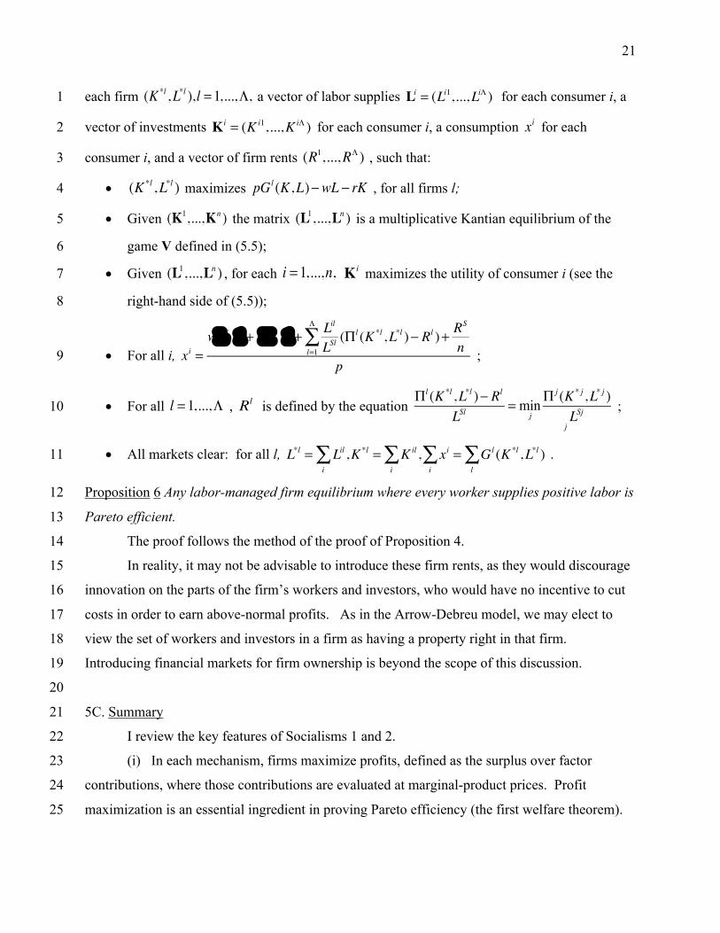
21
each firm a vector of labor supplies for each consumer i, a 1
vector of investments for each consumer i, a consumption for each 2
consumer i, and a vector of firm rents , such that: 3
• maximizes , for all firms l; 4
• Given the matrix is a multiplicative Kantian equilibrium of the 5
game V defined in (5.5); 6
• Given , for each maximizes the utility of consumer i (see the 7
right-hand side of (5.5)); 8
• For all i, ; 9
• For all , is defined by the equation ; 10
• All markets clear: for all l, . 11
Proposition 6 Any labor-managed firm equilibrium where every worker supplies positive labor is 12
Pareto efficient. 13
The proof follows the method of the proof of Proposition 4. 14
In reality, it may not be advisable to introduce these firm rents, as they would discourage 15
innovation on the parts of the firm’s workers and investors, who would have no incentive to cut 16
costs in order to earn above-normal profits. As in the Arrow-Debreu model, we may elect to 17
view the set of workers and investors in a firm as having a property right in that firm. 18
Introducing financial markets for firm ownership is beyond the scope of this discussion. 19
20
5C. Summary 21
I review the key features of Socialisms 1 and 2. 22
(i) In each mechanism, firms maximize profits, defined as the surplus over factor 23
contributions, where those contributions are evaluated at marginal-product prices. Profit 24
maximization is an essential ingredient in proving Pareto efficiency (the first welfare theorem). 25
(K *l ,L*l ),l = 1,...,Λ, Li = (Li1,...,LiΛ )
Ki = (Ki1,...,KiΛ ) xi
(R1,...,RΛ )
(K *l ,L*l ) pGl (K ,L)−wL − rK
(K1,...,Kn ) (L1,...,Ln )
(L1,...,Ln ) i = 1,...,n, Ki
xi =wLi ⋅1+ rK i ⋅1+
l=1
Λ
∑ Lil
LSl(Πl (K *l ,L*l )− Rl )+ R
S
np
l = 1,...,Λ Rl Πl (K *l ,L*l )− Rl
LSl= min
j
Π j (K * j ,L* j )LSj
j
L*l = Lili∑ ,K *l = Kil
i∑ , xi
i∑ = Gl (K *l ,L*l )
l∑
22
But it is also an informal proxy for believing that the mechanism will encourage technological 1
innovation, although this is not modeled in the static environments postulated here. 2
(ii) In both variants, the equilibria are Pareto efficient. Resource allocation is 3
decentralized by the existence of markets and competitive prices, and optimization by 4
individuals and firms. Individual optimization might be either in the manner of Nash, or in the 5
manner (of several versions) of Kant. 6
(iii) Social democracy (Socialism 1) extends the first welfare theorem to apply to 7
equilibrium allocations for any redistribution of income implemented by a linear income tax and 8
demogrant. Avoiding the deadweight loss of taxation is achieved by cooperation, modeled as 9
additive Kantian optimization of workers and investors in the determination of their factor 10
supplies, to be contrasted with the inefficiency of linear taxation under capitalism, which is due 11
to Nash optimization by workers. Except to the extent that incomes are redistributed via 12
taxation, the economic surplus is defined as conventional profits, and is distributed to owners of 13
firms. 14
(iv) Under Socialism 2, of this section, the firm is conceptualized as owned by workers 15
and investors, who share in conventional profits after rental payments are paid to investors and 16
wages are paid to workers. There is a unidimensional family of equilibria, indexed by the share 17
of profits that is allocated to workers. In general, workers and investors may be treated 18
asymmetrically. Pareto efficiency is accomplished via cooperation, modeled as multiplicative 19
Kantian optimization8. I do not have a method of income taxation that will be Pareto efficient 20
for Socialism 2. 21
22
23
6. On the treatment of capital owners 24
In defining these socialist variants, I have respected the distinction made in the Arrow-25
Debreu model between owners of firms and suppliers of capital to the firm. Both profits and 26
factor payments to capital suppliers appear as capital income in the US national accounts, 27
although they are different kinds of income, both legally and conceptually. Their different legal 28
status is shown by the fact that firm owners only receive their shares of profits after factor 29
8 An earlier formulation of a worker-ownership equilibrium is due to Jacques Drèze (1993). In his model, workers maximize in the Nash manner. The equilibrium is also Pareto efficient.
23
payments have been made. Owners are the residual claimants, who stand behind factor 1
suppliers, in the queue whose members divvy up firm income. 2
One might wish to respect a distinction, in thinking about socialism, between firms that 3
are created by individuals, and are not incorporated, and publicly-held corporations. For the 4
first kind of firm, one might be more inclined to think of profits accruing to the owner as an 5
entitlement, a return to entrepreneurial talent. Owners of corporate shares, however, have not in 6
general contributed any entrepreneurial talent to the firm – indeed, whether a corporate investor 7
buys shares or bonds, and thereby becomes either an owner or a factor supplier to the firm, may 8
be due to preferences for risk rather than to having any particular role in the firm’s actions. 9
One possibility for a conception of socialism would be as a regime that encourages the formation 10
of small firms, which would remain privately owned until a certain level of sales is reached, at 11
which time the firm must be transformed into a public firm of the kind described in the l-sharing 12
economy. When that level of sales is reached, the firm would be purchased from the private 13
owner by the state: after that, the distribution of firm income would change as described in 14
section 5, but the former owner might well be hired to manage the new public firm, given her 15
superior knowledge of the firm’s technology and market. 16
The distinction between firm owners and suppliers of capital is probably also important 17
historically. At the time Marx wrote, the distinction may not have been as important as it is 18
today, because the middle class was much less wealthy in the early nineteenth century. It was 19
likely the case that firm owners were largely entrepreneurs, and investors were members of the 20
landed gentry. The more undeserving of these two groups would appear to be the aristocrats, 21
who were searching for profitable returns on incomes that came from landed property ultimately 22
derived from regal distributions to nobility in times past. The twentieth century saw the advent 23
of a patrimonial middle class, as described by Piketty (2015), a middle class he defines as 24
comprising the fiftieth to ninetieth, or perhaps ninety-ninth centiles of the distribution of income 25
or wealth. The income and wealth of this class are due more to the productive contributions of 26
its members than was the income of the aristocracy a return to its members’ productive 27
contributions. Of course, the wealth of the middle class must be invested productively in any 28
efficient economy, and returns to owners will accrue. Thus, unless one conceives of socialism as 29
coming about through a revolution in which the wealth of citizens is confiscated by the state – 30
and very few of those who call themselves socialist today would advocate this – one must pay 31

24
serious attention to providing incentives for citizens to invest their wealth productively. These 1
incentives exist in the models that I have proposed. 2
Given that a large class of citizens will be investors (roughly speaking about 50% of the 3
households in an advanced economy, because in most advanced capitalist countries, those in the 4
top half of the wealth distribution own virtually all the financial wealth), the extent to which 5
(these variants of) socialism would redistribute income from capital to labor is uncertain and 6
important. The uncertainty is clear; the importance derives from the fact that surely the most 7
disadvantaged in society are those with little or no wealth, whose incomes come solely from 8
labor. Although socialism, with its cooperative ethos, should give priority to investment that will 9
augment the skills and earning power of the disadvantaged, we can suppose that class differences 10
will continue to remain between those whose incomes come primarily from labor, and those 11
whose incomes have a significant capital component, and membership in these classes will 12
therefore continue to be closely correlated to social and economic advantage in family 13
background. Although I have not here discussed here what constitutes socialist justice – my 14
views on that are presented in Roemer (2017) --that justice is roughly defined by the elimination 15
of disadvantage due to the luck of the birth lottery. See section 10 below. It is for this reason 16
that the partition of income between capital and labor income will remain important. That 17
partition will cease to be of ethical concern only when there is little correlation between the 18
source of a person’s income and the degree of social/economic disadvantage of his background. 19
20
7. Is Kantian optimization credible behavior, or simply a mathematical curiosum? 21
The three pre-requisites for a group of individuals to optimize in the Kantian manner are 22
desire, understanding, and trust. People must desire to cooperate, because they see their 23
situation as one of solidarity, meaning they face a common economic problem (the struggle 24
against Nature) whose solution will require cooperation. Secondly, they must understand that 25
Kantian optimization can lead to good (efficient) solutions to the economic problem. Third, 26
each must trust that others will optimize in the Kantian manner if he/she does, so that the 27
Kantians will not be taken advantage of by Nash optimizers, who can always benefit as 28
individuals, at least in the short run, by playing Nash against the Kantian crowd. If desire, 29
understanding and trust exist, groups of economic agents may entrust decisions (such as optimal 30
investments or supplies of labor) to organizations that represent them, such as unions, which can 31

25
carry out the Kantian optimization for them. Indeed, the success of the Nordic social 1
democracies depended on strong centralized labor unions, which in their tripartite negotiations 2
with capitalists and government may have proposed Kantian-optimal strategies for workers (this 3
is a conjecture for further research). 4
We know that ethnic, linguistic, and religious heterogeneity frustrate the realization 5
among individuals that they face a situation of solidarity, and many have argued that the 6
homogeneity of Nordic populations along these dimensions contributed to the success of social 7
democracy, because of the relative ease of establishing trust in a homogeneous group. 8
The mathematical similarity between Nash and Kantian equilibrium of agents is that each 9
agent chooses a preferred action in a set of counterfactual strategy profiles in the game, and 10
equilibrium obtains when all agents agree upon what the most preferred strategy profile is. The 11
difference between Nash and Kant protocols is in the specification of the counterfactual sets of 12
strategy profiles. In Nash optimization, each agent inspects a different set of counterfactual 13
profiles, while in Kantian optimization, all agents inspect the same counterfactual set. Thus, 14
Kantian optimization builds in symmetry that does not exist in Nash optimization. It is this 15
symmetry that holds the ethical appeal of Kantian optimization: for fairness, in our minds, is 16
deeply associated with symmetrical treatment. This is why I suggest that if citizens acquire an 17
understanding of their solidaristic situation, and thereby desire to cooperate, the technology of 18
Kantian optimization will become an ethically attractive optimization protocol. 19
20
8. Public bads, public goods and efficiency 21
In this section, I show that Kantian optimization in these blueprints may enable us to 22
deal efficiently with the production of public goods and public bads -- without regulation or 23
imposing effluent fees, in the case of public bads, and without state financing, in the case of 24
public goods. I will display two examples. 25
26
A. Profit maximization may engender public bads 27
28
The socialist blueprints I have offered depend, for their efficiency results, on the 29
maximization of profits by the firm. I have already mentioned that socialists may bridle at the 30
idea that investors should be treated similarly to workers in an advanced socialist economy. 31
26
They may likewise bridle at the idea that profit maximization is so central to these models, 1
because we rightly associate profit maximization with many deleterious practices – employing 2
child labor, polluting, or running assembly lines at a breakneck pace. 3
I believe the deleterious practices that accompany profit maximization in capitalist (and 4
twentieth century socialist) economies must be controlled by recognizing that the public bads, 5
like the ones mentioned in the last paragraph, enter the utility functions of citizens. One can 6
ask whether Kantian optimization can provide a satisfactory solution to the problem of negative 7
externalities that accompany profit maximization, through utility maximization of consumers. 8
To study this, I postulate a utility function of the form , where y is the total 9
product, and utility is decreasing in y. Thus, think of industrial pollution or the speed of the 10
assembly line as being a monotone increasing function of output. A standard approach would be 11
to regulate firms, or to charge emission fees. We can also, however, achieve efficiency, in some 12
cases, via Kantian optimization. 13
We first characterize Pareto efficiency for an economy where total output is a proxy for 14
the level of the public bad that firms will produce if they are not otherwise constrained. 15
16
Proposition 7 Consider the economic environment where production uses labor and 17
capital inputs, and preferences are defined over the vectors as above, and 18
preferences and production are convex. Then an interior allocation is Pareto efficient if and 19
only if: 20
21
22
(8.1) 23
Proof: 24
The claim is proved by solving the program: 25
26
ui (xi ,Li ,Ki , y)
{(ui ),G,n}
(xi ,Li ,Ki , y)
(i) for all i, u3i
u2i =
G2
G1
and (ii) for all i, − u1i
u3i =
1G1
+ u4j
u3j
j∑ .
27
(8.2) 1
The (dual) KKT conditions for the solution are precisely (i) and (ii) as stated in (8.1). ■ 2
3
Let’s now insert the public bad into a social-democratic economy. We continue to define 4
a social-democratic equilibrium with taxation exactly as in section 4. Now the analog to the 5
game W defined in equation (4.1) has payoff functions: 6
. (8.3) 7
The condition for to be an additive Kantian equilibrium of this game is: 8
(8.4) 9
In like manner, the condition for to be an additive Kantian equilibrium of the 10
game V, modified from (4.2), is: 11
. (8.5) 12
Noting that these equations can be written: 13
, (8.6) 14
we deduce that condition (i) of Proposition 7 holds. Next, write (8.5) as: 15
16
. (8.7) 17
Now suppose that . Then the second equation in (8.6) 18
becomes , and so the numbers are invariant across i. Consequently 19
maxu1(x1,L1,K1, y)s.t.j >1⇒ (u j (x j ,Lj ,K j , y) ≥ k j )xS ≤G(KS ,LS ) ≡ y
W i (L1,L2,...,Ln ) = ui ((1− t)(wLi + rK i + θi (pG(K *,L*)− rK * −wL*)
p+
tnwLS + rK S +Π(K *,L*)
p,Li ,Ki ,G(KS ,LS ))
(L1,...,Ln )
u1i ⋅wp+ u2
i + u4i G2n = 0.
(K1,...,Kn )
u1i ⋅ rp+ u3
i + u4i G1n = 0
G2 ⋅(u1i + nu4
i ) = −u2i and G1 ⋅(u1
i + nu4i ) = −u3
i
− u1i
nu3i =
1nG1
+ u4i
u3i
ui (xi ,Li ,Ki , y) = xi − hi (Li ,Ki )− f (y)
G1 ⋅(1− n ′f (y)) = −u3i u3
i

28
(since ), we can add equations (8.7) to get . This is condition (ii) for 1
Pareto efficiency from Proposition 7. To summarize: 2
3
Proposition 8 If , then social democratic equilibrium 4
(Socialism 1), amended to include the disutility associated with a public bad that accompanies 5
production, is Pareto efficient at any tax rate . 6
7
Although Proposition 8 has a restrictive premise, it shows there is a potential for Kantian 8
optimization to eliminate the deadweight loss of taxation and the inefficiency associated with 9
negative production externalities at the same time. What’s required is that factor suppliers take 10
into account the negative externality that is a function of the total product that their factor 11
supplies engender. See (8.3). In particular, we do not restrict the firm’s profit-maximizing 12
behavior through regulation. Rather, the otherwise deleterious effects of that behavior are 13
controlled by cooperation among workers and investors in their factor supply behavior. 14
15
B. Production of a private and public good 16
Assume that there is a private good produced by the production function G, and a public 17
good, produced by the production function H, also using capital and labor. Preferences of 18
consumers are defined on vectors where z is the amount of the public good 19
produced. In general, consumers will expend labor and invest capital in both the private-good 20
firm operating G, and the public-good firm operating H. We first characterize Pareto 21
efficiency. 22
Proposition 9 Let be consumer i’s consumption, supply of labor to the 23
private and public good firms, respectively, and her supply of capital to the private and public 24
good firms, respectively. Let z be the level of the public good. An interior allocation is Pareto 25
efficient if and only if9: 26
27
9 In the utility function,
u1i ≡ 1 − u1
u3= 1G1
+ u4i
u3i
i∑
ui (xi ,Li ,Ki , y) = xi − hi (Li ,Ki )− f (y)
t ∈[0,1]
(xi ,Li ,Ki , z)
(xi ,L1i ,L2
i ,K1i ,K2
i )
Li = L1i + L2
i and Ki = K1i + K2
i .

29
(8.8) 1
Proof: Appendix. 2
Conditions (i) and (ii) state that the marginal rates of substitution between labor 3
(capital) and consumption equal the required marginal rates of transformation, and conditions 4
(iii) and (iv) are the Samuelson conditions with respect to the public good. 5
We will now define an equilibrium for the social-democratic economy with a public 6
good. There are two firms, one producing the private good, the other producing the public good, 7
both using capital and labor. Workers and investors will make their decisions conventionally 8
with regard to labor and capital supplies. Each citizen will contribute to the financing of the 9
public good: the vector of such contributions will be a multiplicative Kantian equilibrium of the 10
relevant game. 11
Denote the share of citizen i in the private (public) firm by and profits in the 12
private (public) firm by . The price vector will be denoted where q is the 13
price of a unit of the public good. I define the payoff function for consumer i, which is, as 14
always, the utility of the consumer at the allocation. The vector is the citizens’ 15
contributions to financing the public good. If the citizens contribute in total , then the public 16
good will be financing at level : 17
18
. (8.9) 19
In the above, the worker’s labor supply is , where is her labor supply to 20
the private (public ) firm. The worker is indifferent with respect to how her total labor supply is 21
allocated between the firms. Likewise, the investor’s investment in the two firms is 22
. 23
We now define: 24
Definition 6 A social-democratic equilibrium with a public good is a price vector , an 25
allocation , factor demands for the private-good firm, factor 26
(i)(− u2i
u1i = G2 ), (ii)(∀i)(−
u3i
u1i = G1) (iii) u4
i
u2i
i∑ = − 1
H2
, and (iv) u4i
u3i
i∑ = − 1
H1
.
θ i (ϕ i )
ΠPr (ΠPb ) (p,w,r,q)
(C1,C 2,...,Cn )
CS
CS / q
V i (C1,C 2,...,Cn ) = ui ((wL1i + rK1
i + θiΠPr (K1*,L1
* )+ϕiΠPb (K2*,L2
* )−Ci
p),Li ,Ki ,C
S
q)
Li = L1i + L2
i L1i (L2
i )
Ki = K1i + K2
i
(p,w,r,q)
(xi ,L1i ,L2
i ,K1i ,K2
i )i=1,...,n (K1*,L1
* )

30
demands for the public-good firm, a vector of contributions , and a level of 1
the public good z, and such that: 2
• the private-good firm demands capital and labor to maximize profits 3
, 4
• the public-good firm demands capital and labor to maximize profits 5
, 6
• given , is a multiplicative Kantian equilibrium of 7
the game V defined in (8.9), 8
• given , for every consumer i, maximizes 9
where 10
• , 11
• and 12
• all markets clear: 13
Note that this equilibrium is an instance of the voluntary production of a public good – via 14
Kantian optimization. 15
16
Proposition 10 Any interior allocation at a social-democratic equilibrium with a public good is 17
Pareto efficient. 18
Proof: 19
1. By profit maximization, . 20
2. The f.o.c.’s for being a multiplicative Kantian equilibrium of the public-21
good-financing game are: 22
or . (8.10) 23
3. Adding equations (8.10) and using step 1 to eliminate p and q, we have: 24 25
(K2*,L2
* ) (C1,...,Cn )
(K1*,L1
* )
pG(K ,L)− rK −wL
(K2*,L2
* )
qH (K ,L)− rK −wL
(Li ,Ki ,ΠPr ,ΠPb ) (C1,...,Cn )
(C1,...,Cn ) (Li ,Ki ) ui (xi ,Li ,Ki ,CS
q)
xi = wLi + rK i + θiΠPr (K1
*,L1* )+ϕiΠPb (K2
*,L2* )−Ci
p
qz = CS ,
K * = K1S ,L1
* + L2* = LS , xS = G(K1
*,L1* ), and z = H (K2
*,L2* ).
wp= G2 , r
p= G1,
wq= H2, and r
q= H1
(C1,...,Cn )'s
(∀i)(−u1i Ci
p+ u4
i CS
q= 0)
u4i
u1i =
qpCi
CS

31
. (8.11) 1
4. Consumer optimal choice of gives: 2
. (8.12) 3
5. Conditions (8.8) characterizing Pareto efficiency in this economic environment follow 4
immediately from steps 4 and 5. ■ 5
6
Asocial-democraticequilibriumwithapublicgoodis,infact,aLindahlequilibrium.7
Toseethis,notethataLindahlequilibriumisdefinedasfollowsforthisenvironment.8
9
Definition7A Lindahl equilibrium is a price vector , personalized prices 10
for the public good, an allocation , factor demands for the 11
private firm, factor demands for the public-good firm, a vector of contributions 12
, and a level of the public good z, and such that: 13
• the private-good firm demands capital and labor to maximize profits 14
, 15
• the public-good firm demands capital and labor to maximize profits 16
, 17
• given , , where 18
• , 19
• and 20
21
• all markets clear: 22
23
WeshowthatanyLindahlequilibriumisasocial-democraticequilibriumwitha24
publicgood.ForlettheLindahlequilibriumbegiven,asdenotedindefinition7.Define25
u4i
u1i
1
n
∑ = G1H1
= G2
H2
(Li ,Ki )
for all i, − u2i
u1i = G2 and − u3
i
u1i = G1
(p,w,r,q) (q1,...,qn )
(xi ,L1i ,L2
i ,K1i ,K2
i )i=1,...,n (K1*,L1
* )
(K2*,L2
* )
(C1,...,Cn )
(K1*,L1
* )
pG(K ,L)− rK −wL
(K2*,L2
* )
qH (K ,L)− rK −wL
(Li ,Ki ,ΠPr ,ΠPb ) (xi ,Li ,Ki , z) maximizes ui (xi ,Li ,Ki , z)
xi = wLi + rK i + θiΠPr (K1
*,L1* )+ϕiΠPb (K2
*,L2* )− qiz
p
qi = q,i∑
K * = K1S ,LS = L1
* + L2* , xS = G(K *,L*), and z = H (K2
*,L2* ).
32
andso .Notethattheconsumer’sfirst-orderconditionforthe1
maximizationofutilitywithrespecttozintheLindahlequilibriumis:2
. (8.13) 3
But equation (8.13) is equivalent to : 4 5
(8.14) 6
7
whichisthefirst-orderconditionformultiplicativeKantianoptimizationinthesocial-8
democraticequilibrium,givenconcavity(seeequation(8.10)).Thisprovestheclaim.9
Itimmediatelyfollowsthatthesocial-democraticequilibriumwithapublicgood10
existsunderstandardconvexityconditions,becauseitiswell-knownthatLindahl11
equilibriumexistsundersuchconditions(seeFoley[1970]).Onedrawbackofthe12
Lindahlequilibriumisthatthepersonalizedprices arenotobservedonanymarket,so13
theLindahlequilibriumisnotentirelydecentralized.Byreplacingthepersonalprices14
withKantianoptimization,wesucceedincompletelydecentralizingtheLindahl15
equilibrium.16
ItisnoteworthythatSilvestre(1984)provedthat,inanyeconomywithapublic17
good,Paretoefficiencyplustheconditionthatnoconsumerwoulddesiretore-scalethe18
vectorofcontributionstothepublicgooddownwardtogethercharacterizeLindahl19
equilibrium.Iftheallocationisinterior,andtheeconomyisdifferentiable,thenitisalso20
truethatnoconsumerwoulddesiretore-scalecontributionstothepublicgoodupward.21
Therefore,Silvestre(1984)effectivelyprovedthatanyLindahlequilibriumisasocial-22
democraticequilibriumwithapublicgoodavantlalettre.23
24
9. Simulations of socialist income distributions 25
It is important to emphasize that the advantage, in terms of reduction of income 26
inequality, of the laissez-faire socialist variant of social democracy, and of the asymmetric 27
sharing economies, only exists when the production function of the firm is strictly concave. For 28
suppose that, to the contrary, G is homogeneous of degree one – that is, production enjoys 29
Ci = qiz CS = qz
qi
p= u4
i
u1i
u4i
u1i =
qpCi
CS
{qi}

33
constant returns to scale. Then the asymmetric sharing equilibrium and the worker-ownership 1
equilibrium are identical to the capitalist equilibrium with zero taxation. In other words, what 2
those variants of socialism do is distribute profits in proportion to factor contributions; but when 3
there are constant returns to scale, profits are zero in these models, there is no surplus to 4
distribute, and so capitalism with zero taxation is equivalent to both socialist variants. 5
Democratic-socialist equilibria will differ, however, from capitalist equilibrium if the tax rate is 6
positive, because workers optimize in different ways (Nash and Kant) in their labor-supply 7
decisions in the socialist and capitalist models. 8
I am unsure how best to characterize returns to scale for the economy as a whole. There 9
is certainly a tradition of assuming that returns are constant10. In this section I will simulate three 10
models in which I assume decreasing returns so that profits are positive. These are: capitalism 11
with a positive tax rate, social-democracy with various positive tax rates, and the sharing 12
economy with various distributions of the capital endowment. 13
I assume a Cobb-Douglas production function: 14
, some , (9.1) 15
and a quasi-linear utility function 16
(9.2) 17
where x is income measured in thousands of dollars per annum, is labor time expended in a 18
calendar year measured in (full-time equivalent) years, and h is the elasticity of substitution of 19
labor time with respect to the wage11. We assume that household capital is inelastically supplied. 20
Workers differ in the efficiency units of their labor. The labor efficiency of a worker is s, 21
measured in some normalized amount of output that the worker can produce with one year’s 22
10 It would be a false inference to argue that, because reported profits in the national accounts are positive, therefore returns to scale must be decreasing. Reported profits are different from neoclassical profits. One important reason for the difference is that most firms own some of their capital stock. Were we to subtract imputed rents payments on owned capital from firm profits, it is conceivable profits would be zero, in line with the constant-returns assumption. Of course, the main reason that profits are positive is monopoly pricing by firms, perhaps related to their having increasing returns. For instance, Stiglitz (2019), argues that non-competitive pricing is a central cause of inequality today. 11 We need not suppose that preferences have capital lent to firms as an argument. Individuals supply their entire capital endowment to the firm.
G(K ,L) = AK γ Lϕ−γ γ <ϕ <1
u(x,ℓ) = x − b ℓ1+1/η
1+1/η
ℓ

34
work. I assume a lognormal distribution of s in the population, with a mean of unity and a 1
median of 0.85; that is 2
, (9.3) 3
where F is lognormal. It will be assumed that the share of society’s capital endowment owned 4
by a worker of type s is given by an increasing function : in reality, this may be only 5
approximately correct. It is assumed every member of the population is a worker. Thus: 6
, (9.4) 7
and the amount of a worker’s capital endowment is , where is capital per worker. The 8 number of workers is n, total capital stock is . 9 10 The parameters of the model are the functions , and the numbers 11
. 12 13
A. Calibration 14
15
For the calibration of the model, we assume a competitive capitalist economy with a linear 16
income tax at rate Total wealth will be total financial wealth in the US in 2016. The 17
distribution of total wealth is computed from the data set of G. Zucman (2017), which provides a 18
cumulative distribution function of financial wealth of US adults12. Total financial wealth is 19
$55.6 trillion. I assume this is the value of capital invested in the corporate sector. Value 20
added in the corporate sector in 2017 was $9.5 trillion13: this is the ‘GDP’ of the economy 21
that I study14. 22
12 Total financial wealth is the sum of equities, fixed-income assets, pensions, and life insurance. The file from Zucman (2017) is “USdina2016.dta,” which gives the empirical distribution of financial wealth. 13 From National Income and Product Accounts (NIPA), Table 1.14, line 17. 14 Zucman’s data on financial wealth are for a sample of the population of US adults. The total population of US adults in 2016 was 238 million. Thus, average capital per adult was $233 thousand. However, in the model I take the population of workers to be 127 million, and I assume they own all the capital. Capital per worker is thus $438,000. This renders the worker in the model wealthier than he or she is reality, and this should be recalled when I present below Gini coefficients of the distribution of income with various tax rates.
sdF(s) = 1, F(0.85) =0
∞
∫ 0.5
k(⋅)
k(s)dF(s) = 10
∞
∫
k(s)k kKtot = nk
F(⋅) and k(⋅)(A,b,ϕ,γ ,η,n,Ktot )
t = 30%.
y =

35
I take and I let , although there is much debate about the 1
appropriate value. Finally, the average US worker works 44 hours per week (amortized over 52 2
weeks). If we take one FTE year of labor to be 2080 hours (that is, hours), then total 3
labor time expended is: 4
(9.5) 5
In the continuous version, the set of workers is a continuum of size 1; however, to calibrate the 6
model I take the number of workers to be n = 127 million (workers in private industry, Bureau of 7
Economic Analysis). The calibration task is to compute the function and the numbers 8
; other parameters have been set above. We assume the price of output is unity, and the wage for 9
one unit of labor in efficiency units, and the rental rate for capital, are , respectively. 10
(i) The firm’s problem is to demand capital and labor to 11
(9.6) 12
where L is labor in efficiency units. Profits at the optimum are denoted . 13 14
The f.o.c.’s for profit-maximization are: 15 16
(9.7) 17
where . Denote the solution by . Profits are . Pre-tax capital 18 income is and labor income is . Capital’s pre-tax share is 19
. 20 21 (ii) The problem of a worker of type s is to choose to : 22
(9.8) 23
where is the after-tax income of a worker with skill level s. 24
An explanation of the formula for income in program (9.8) is required. The Arrow-25
Debreu model assumes that each consumer i is endowed with a share of the firm and some 26
capital. In reality, households use their capital to purchase corporate bonds and equity. Suppose 27
a worker of type s invests his wealth in both bonds and equity: we can write 28
γ = 0.333 ϕ = 0.93. η = 0.1
40 × 52
ℓtot = 4440n = 1.1n.
k(⋅) (A,b)
(w,r)
maxG(K ,L)−wL − rK ,
Π*
w = (ϕ − γ )yL
, r = γyK,
y = G(K ,L) (K *,L*) (1−ϕ )yrK * +Π* = (1−ϕ + γ )y, wL*
1−ϕ + γ = 0.40
(x(s),L(s))
maxu(x(s), L(s)s)
s.t.
x(s) = (1− t)(wL(s)+ rk(s)k + k(s)Π*)+ tnG(K *,L*)
x(s)
θi

36
1
. (9.9) 2
The firm pays rents to bondholders, and profits to shareholders. In equation (9.6), should K then 3
be interpreted as the firm’s bond liabilities? No, it should be the firm’s total capital stock – for 4
otherwise, profits will be too large. I will assume that every worker chooses the same ratio of 5
bonds to equities, and so both are proportional to . Thus, in the income 6
formula of (9.8), the worker’s bond income is , and her profit income is , 7
because by the assumption of proportionality, her share of profits is equal to . 8
Consequently, the worker’s (total) capital income is . This approach has two 9
advantages: first, it preserves the neoclassical definition of profits , and second, the rate of 10
return on equity is greater than the rate of return on bonds. In fact, if households invest 11
fractions of their capital in bonds and equity, respectively, then the rate of return on 12
equity will be , which is the equity premium. (Of course, the equity 13
premium here has no economic justification, because risk is not modeled.) 14
15 The f.o.c. under Nash optimization by the worker gives: 16
(9.10) 17
Thus average (per-worker) units of efficiency labor supplied are : 18
(9.11) 19
Furthermore, from (9.5) we have: 20
(9.12) 21
We next compute the function . For this we use the distribution of wealth in 2016, 22
computed (by the author) from Zucman (2017): 23
24 25 26
k(s)k = B(s)+ E(s)
B(s) and E(s) k(s)
rB(s) rE(s)+ k(s)Π*
Π* k(s)
k(s)(rk +Π*)
Π*
β and 1−β
Π*
(1−β)Ktot =1−ϕ(1−β)γ
L(s) = (1− t)wb
⎛⎝⎜
⎞⎠⎟η
s1+η and ℓ(s) = L(s)s
= (1− t)wb
⎛⎝⎜
⎞⎠⎟η
sη .
L(s)dF(s) = (1− t)wb
⎛⎝⎜
⎞⎠⎟∫η
µ1+η where µ1+η ≡ s1+η dF(s).∫
1.1n = L(s)s
dF(s) = (1− t)wb
⎛⎝⎜
⎞⎠⎟∫η
µη where µη ≡ sη dF(s).∫k(⋅)

37
Wealth fractile Fraction of total financial wealth owned by fractile
Bottom half 0.025 .50 - .90 0.261 .90 - .99 0.303 .99 -.999 0.177 .999 -.9999 0.105 .9999 -1.0 0.129
1 Table 1. Wealth shares for various fractiles of the population, computed by the author from 2
Zucman (2017) 3
4 Denote quantile q of the distribution of F by . (For example, the median is .) 5 We compute the values from postulate (9.3) . We now define the 6 function by a piece-wise linear approximation: 7 8 9
10
(9.13) 11
12
We compute the values of so that in each interval , we have the 13
wealth share equals the estimated wealth share from Table 1, and Thus 14
is the ‘share’ of total capital owned by workers of type s. 15
This calibration gives: 16
. (9.14) 17
We now finish the calibration as follows. From (9.12), we compute that: 18
. (9.15) 19
sq s0.5 = 0.85(s0.5 , s0.9 , s0.99 , s0.999 , s0.9999 )
k(s)
k(s) =
a0s, s∈[0, s0.5 )a0s0.5 + a1(s − s0.5 ), s∈[s0.5 , s0.9 )
a0s0.5 + a1(s0.9 − s0.5 )+ a2 (s − s0.9 ), s∈[s0.9 , s0.99 )a0s0.5 + a1(s0.9 − s0.5 )+ a2 (s0.99 − s0.9 )+ a3(s − s0.99 ), s∈[s0.99 , s0.999 )
a0s0.5 + a1(s0.9 − s0.5 )+ a2 (s0.99 − s0.9 )+ a3(s0.999 − s0.99 )+ a4 (s − s0.999 ), s∈[s0.999 , s0.9999 ]a0s0.5 + a1(s0.9 − s0.5 )+ a2 (s0.99 − s0.9 )+ a3(s0.999 − s0.99 )+ a4 (s0.9999 − s0.999 )+ a5 (s − s0.9999 ), s ≥ s0.9999
⎧
⎨
⎪⎪⎪⎪
⎩
⎪⎪⎪⎪
(a0,a1,a2,a3,a4 ,a5 ) (sq , sp )
k(s)dF(s) = 1.0
∞
∫k(s)dF(s)
(a0,a1,a2,a3,a4 ,a5 ) = (0.088, 1.68, 3.94, 23.04, 105.12, 916.49)
wb= 4.289

38
Substituting this ratio into (9.11), we compute , and hence . In 1
equilibrium, we have . Of course, . Now, from the equation: 2
3
(9.16) 4
, we compute From equations (9.7), we compute . That is, 5
the wage for one unit (year) of efficiency labor is about $39,300. Finally, from (9.15) we 6
compute This completes the calibration. 7
Income is defined by the constraint in program (9.8). We check the calculation by 8
checking that incomes add up to GNP, that is, that: 9
10
(9.17) 11
Average income per worker is $74,803, and trillion, as stated above. 12
13 B. Gini coefficient 14
The Gini coefficient of income at this equilibrium is 0.37415. The capitalist equilibrium 15
is Pareto inefficient because of the deadweight loss at positive taxation. 16
17
C. How the Gini coefficient changes with the tax rate in social-democratic equilibrium 18
19
In calibrating the model in section 8A, I took the equilibrium to be that of capitalism with 20
taxation. In particular, we assumed that workers choose their labor supplies according to Nash 21
optimization. (We simply assumed that capital is inelastically supplied.) Thus, the equilibrium 22
calculated in section 8A above is Pareto inefficient due to the deadweight loss of taxation. 23
We next compute the capitalist equilibrium when for the parameterized model. 24
This allocation will be Pareto efficient. As I pointed out earlier16, because the utility function is 25
quasi-linear, as we vary the tax rate in social-democratic equilibrium, none of prices change, nor 26
15 The Gini coefficient is defined as where
16 See the last paragraph of section 4.
Lave = L(s)dF(s)∫ Ltot = nLave
Ltot = L* Ktot = K *
y = A(K *)γ (L*)ϕ−γ
A = 3384. (w,r) = ($39299., 0.057)
b = 9163.
x(s)dF(s) = G(K *,L*).∫y = $9.5
t = 0
12µ
x(s)− x(τ )∫∫ dF(s)dF(τ ),
µ = x(s)dF(s).∫

39
do any labor supplies--all that occurs is a redistribution of income among citizens. Thus, if the 1
capitalist equilibrium when is described by the functions and prices , then 2
income in the social-democratic equilibrium with a tax rate of t is given by: 3
4
. (9.18) 5
Thus, we easily compute the Gini coefficients of income in social-democratic equilibrium as we 6
vary the tax rate. We also present the “99:10 ratio,” “90:10 ratio,” and the “75:10 ratio,” the 7
ratios of total income of workers at various pairs of quantiles. 8
9
10 Table 2. Income Gini coefficients in (Pareto efficient) social-democratic equilibrium as the tax 11
rate varies 12
13
As I pointed out, the total product is invariant with respect to the tax rate. In these 14
social-democratic equilibria, it is . Thus the deadweight loss of output due to 15
taxation in the capitalist model with is . Doubtless the true 16
inefficiency, due to oligopolistic price setting and rent seeking (see Stiglitz [2019])), is 17
considerably greater. 18
Note that the Gini coefficient in (the efficient) social-democratic equilibrium when the 19
tax rate is 30% is slightly larger than the Gini coefficient in (the inefficient) capitalist 20
equilibrium at that tax rate (which is 0.374). It is interesting to observe what the distribution of 21
welfare (utility) is in latter economy, in comparison with the distribution of welfare in the social-22
democratic equilibrium at various tax rates. 23
t = 0 {L(s),k(s),w,r}
x(s;t) = (1− t)(wL(s)+ rk(s)k + k(s)Π*)+ tnG(Ktot ,Ltot )
$9.70 trillion
t = 30% 9.70 − 9.59.70
= 2.0%

40
In all the figures of this section, I plot the distribution of utility as a function of the 1
quantile of the agent in the distribution of skill (and wealth). See Figure 117. 2
[place Figure 1 about here] 3
4
The allocations in the three social-democratic equilibria plotted in figure 1 are Pareto 5
efficient. We see that at a tax rate of 30% , the social-democratic equilibrium Pareto dominates 6
the capitalist equilibrium. Even at 50% the social-democratic equilibrium Pareto dominates the 7
capitalist equilibrium well into the 99th centile. At a tax rate of 90% the social-democratic 8
equilibrium is massively better for the low skilled than the capitalist equilibrium at 30%, but 9
those with skill level in the top 7% fare worse than in the capitalist equilibrium at 30%. Recall 10
that, due to linear taxation, in all these equilibria, utility is strictly monotone increasing in s and 11
q. Although taxation can sharply reduce income inequality, it never alters the rank of any 12
individual in the income distribution. 13
I now turn to equilibria for the sharing economy. First, I assume the same 14
distribution of financial wealth as in the earlier simulations. By virtue of the quasi-linearity 15
preferences, factor supplies are invariant with , and are exactly the same as those in the 16
social-democratic equilibria: all that changes with is the distribution of income. Table 3 17
presents the Gini coefficient of income as varies. 18
19 Table 3. Gini coefficients of income in the -sharing economy 20
21
[place figure 2 about here] 22
23
17 The kinks in the graphs of figure 1 are due to the piece-wise linear approximation to the distribution of capital.
λ −
λ
λ
λ
λ
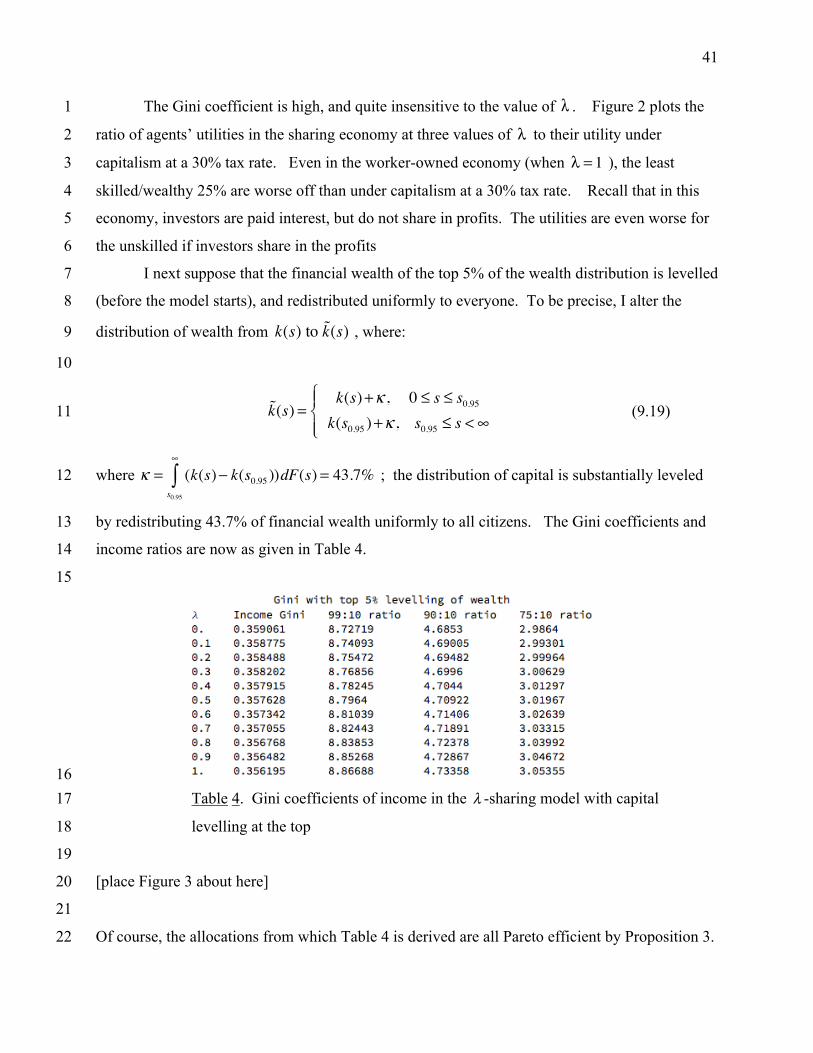
41
The Gini coefficient is high, and quite insensitive to the value of . Figure 2 plots the 1
ratio of agents’ utilities in the sharing economy at three values of to their utility under 2
capitalism at a 30% tax rate. Even in the worker-owned economy (when ), the least 3
skilled/wealthy 25% are worse off than under capitalism at a 30% tax rate. Recall that in this 4
economy, investors are paid interest, but do not share in profits. The utilities are even worse for 5
the unskilled if investors share in the profits 6
I next suppose that the financial wealth of the top 5% of the wealth distribution is levelled 7
(before the model starts), and redistributed uniformly to everyone. To be precise, I alter the 8
distribution of wealth from , where: 9
10
(9.19) 11
where ; the distribution of capital is substantially leveled 12
by redistributing 43.7% of financial wealth uniformly to all citizens. The Gini coefficients and 13
income ratios are now as given in Table 4. 14
15
16 Table 4. Gini coefficients of income in the -sharing model with capital 17
levelling at the top 18
19
[place Figure 3 about here] 20
21
Of course, the allocations from which Table 4 is derived are all Pareto efficient by Proposition 3. 22
λ
λ
λ = 1
k(s) to !k(s)
!k(s) =k(s)+κ , 0 ≤ s ≤ s0.95k(s0.95 )+κ , s0.95 ≤ s < ∞
⎧⎨⎪
⎩⎪
κ = (k(s)− k(s0.95 ))dF(s) = 43.7%s0.95
∞
∫
λ

42
Figure 3 plots the utility ratios between these sharing economies and capitalism at a 30% tax 1
rate. Now, almost all agents except at the very bottom and top of the distribution of skill/wealth 2
do better in the sharing economy. It is interesting to note that the very unskilled have higher 3
utility in the investor-owned sharing economy, when , than in the worker-owned 4
economy, when . The reason is that the capital they receive from the redistribution of 5
wealth at the top is more valuable than their labor. 6
7
10. What does it mean to be socialist today? 8 9 Clearly a limitation of my analysis is its classical assumption that technology is 10
characterized by constant or decreasing returns to scale. A proper treatment of what socialism 11
would require when increasing returns to scale (IRS) holds is a project that, I hope, can be 12
informed by this classical analysis. I have not attempted this, for lack of a simple, canonical 13
equilibrium model of IRS. 14
One could attempt to answer the question posed in this section’s title by asking what 15
conception of a cooperative economy best fits the most prominent classical definition of 16
socialism, which I take to be Karl Marx’s. Marxian socialism is an economic system in which 17
‘each works according to his ability and is paid according to his work.’ Although Marx did not 18
go into the institutional details of how this instruction would be implemented, most Marxists 19
assumed that it would entail state ownership of firms (the means of production), and 20
remuneration of labor in proportion to skill. At least such was the case during the Soviet era. 21
The entire economic product would be so distributed, after a share had been reserved for 22
investment. Not only firms but capital would be state-owned, so the only privately-owned 23
production factor would be labor power. 24
What was the ethical justification of such a regime? It was that capital comes into being 25
‘dripping from head to foot, from every pore, with blood and dirt (Marx[1965, p.760]).’ Thus, 26
capital (in the pre-capitalist history of Britain, at least according to Marx’s research in the British 27
Museum) was not accumulated through honest work, from a decision to save from earnings, but 28
from plunder, enclosure, royal decree, and conquest. And in the capitalist era, capital grew 29
through the exploitation of labor. Marx, however, viewed workers as the rightful owners of 30
their labor power, and hence the just or fair division of the economic product was in proportion 31
λ = 0
λ = 1

43
to labor expended (measured in efficiency units), after the state, presumably, had taken a share of 1
the product for investment. 2
The nature of modern advanced economies today is, however, very different from Marx’s 3
vision of early capitalist Britain – we need not debate here whether his vision was historically 4
accurate, for it was, in any case, the vision that inspired Marx’s conception of socialism. 5
According to my calculation, based upon the financial wealth data in Zucman (2017), the 6
financial wealth of the Piketty’s middle class in the United States, those occupying the 50th to 7
90th centiles of the financial wealth distribution, comprises 26% of total US financial wealth, and 8
if we include the upper middle class, those in the 90th to 99th centile, the financial wealth share 9
rises to 56%18. It cannot be argued that this wealth came about through plunder, conquest, and 10
enclosure: rather, the default assumption must be that most of it came about through investment 11
from saved earnings and inheritance. 12
One can still maintain that this middle-class wealth has not been justly acquired, but to do 13
so, one must employ a (Rawlsian) argument quite different from Marx’s blood-and-dirt 14
argument. The earning capacity that people acquire in capitalist societies is massively influenced 15
by the families into which they are born, and that circumstance, according to Rawls, is morally 16
arbitrary. People neither justly benefit nor suffer due to morally arbitrary circumstances that 17
characterize their natural and social environments. This view is more radical than Marx’s, 18
because it does not treat even a person’s labor power and skill as justly owned by the person, to 19
the degree that the development of that skill is a consequence of a highly-resourced upbringing 20
and education that the person may have had by virtue of the luck of the birth lottery. It is also, 21
however, less radical than Marx’s view, because it does not treat all private wealth accumulation 22
as immoral: if a person comes by her skills and earning capacity in an environment of equal 23
opportunity, then her decision to save some of her earnings in order to optimize her lifetime 24
consumption path is ethically protected19. I would still argue that inheritance must be sharply 25
restricted (as did James Meade), for the differential wealths of the current generation, even if 26
justly acquired, would destroy equality of opportunity for the next generation, were inheritance 27
18 The top 1% owns 42% of financial capital, and the bottom half, 2%. Financial wealth does not include the value of residences. 19 Rawls, in particular, was supportive of James Meade’s (1964) conception of a property-owning democracy.

44
not to be restricted. See Piketty (2015, chapter 11) for an historical analysis of the importance of 1
inheritance in generating the present distribution of wealth. 2
As I mentioned in section 1, Cohen (2009) has argued that the proper construal of 3
socialist ethics, at the beginning of the twenty-first century, is that income differentials traceable 4
to differential luck (in large part, the luck of the birth lottery) should be eliminated, but 5
differential incomes traceable to different choices, sterilized of luck, are permissible. If one 6
wishes to think of Cohen’s proposal as a generalization of Marx’s view, one would say that for 7
Marx the main circumstance (morally arbitrary luck) was the ownership of capital, and hence 8
(Marx believed) socialism required the elimination of differential capital ownership via state 9
ownership. Perhaps more to the point, rather than proposing an ethical argument, he claimed, 10
willy-nilly, that state ownership was next on the historical agenda. 11
If socialism is to be constructed from the initial conditions of existing capitalism, then 12
one must design rules that view the wealth of the middle class as entitled to remuneration, while 13
at the same time recognizing that wealth has been acquired in a regime characterized by sharp 14
inequality of opportunity. Of the variants of socialism that I have presented, Socialism 1 (social 15
democracy with taxation, sections 4 and 8) has the advantage that income taxation can be 16
implemented with Kantian optimization, engendering a large range of income Gini coefficients, 17
without sacrificing efficiency. 18
To achieve acceptable income-Gini coefficients in the sharing economy (Socialism 2), we 19
need either a significant redistribution of financial wealth, as I have simulated in section 9, or 20
income taxation – and the latter, as far as I know, will be inefficient. However, we should not 21
discard the blueprint of the sharing economy, because of the importance of the cooperative ethos 22
to socialism, and the possible dynamic interaction between that ethos and property relations. 23
Is it psychologically feasible for some members of a society to desire to cooperate with 24
others whom they see have much higher incomes? Cohen (2009) writes it is not, and it is hard 25
to disagree20. Thus, for workers and investors to cooperate in the sense that Kantian 26
20 I am taking a liberty here. Cohen (2009, p.35) writes, “We cannot enjoy community, you and I, if you make, and keep, say, ten times as much money as I do, because my life will then labor under challenges that you will never face….” I have substituted ‘cooperate’ for ‘enjoy community’ in this sentence. Arguably, the conditions for Cohen’s communal feeling are more demanding than for cooperation. My justification for this substitution is that cooperation may

45
optimization requires, a quite substantial redistribution of income will be necessary. Indeed, 1
equalizing opportunities for the acquisition of earning power, itself a major project, may be 2
insufficient for ensuring the degree of income equality that would be required to generate the 3
trust needed for workers and investors to optimize in the Kantian manner. 4
I am hesitant to discard Socialism 2 because of considerations of ethos stability that may 5
recommend it over social democracy. The formalized optimizing behavior upon which I have 6
focused may be only the tip of the cooperative iceberg. More generally, one can ask whether 7
the cooperative ethos can thrive with the capitalist allocation rule (of pre-tax income) of 8
Socialism 1. Socialism 2 has the attractive property that the entire product is distributed to the 9
cooperative producers: no class exists that claims part of the product but whose members do not 10
participate in production. I certainly do not fully understand the psychology that will be 11
necessary to maintain the desire, understanding and trust that are the necessary for maintaining a 12
cooperative ethos, but it may be the case that that ethos is more aligned with ‘cooperation in 13
production,’ as occurs in Socialism 2 than with social democracy. 14
Saez and Zucman (2019, chapter 3) relate how, in the period 1930 -1970, a more 15
cooperative ethos existed in the United States than we experience today: the key evidence is the 16
existence of very high, even confiscatory, taxes on the very rich. In 1960, the average tax rate 17
applied to 400 richest Americans was close to 60% of their income; today, it is a little over 20%, 18
lower than the average tax rate experienced by the poorest 50% of households.21 This 19
degeneration of social solidarity could not have occurred without massive re-enforcement of the 20
individualistic ethos in America – corresponding historically to the passage from F.D. Roosevelt 21
to R. Reagan22 and M. Thatcher and its correlated rise in the individualistic ethos. 22
To restate my tentative conclusions, thus risking the danger of boring the reader, they are 23
these. Viewing the socialist allocation rule as distribution of the product in proportion to labor 24
require that people feel they are ‘in the same boat,’ and that feeling may fail to develop between individuals between whom there are very large income differentials. 21 Taxes comprise federal, state, local, property, and estate. See Figure 1.4, Saez and Zucman (2019). 22 Roosevelt said, in a message to Congress, in 1942: “Discrepancies between low personal incomes and very high personal incomes should be lessened; and I therefore believe that in time of this grave national danger, when all excess income should go to win the war, no American citizen ought to have a net income, after he has paid his taxes, of more than $25,000 a year [equivalent to about $1 million in 2019 dollars].” Saez and Zucman (2019, p. 35).

46
expended, after subtracting a share for investment, is only justifiable if the accumulation of 1
private financial wealth is viewed as ethically illicit. In socialist society, this cannot be correct. 2
Individual saving must be legitimate, if social mobility (more generally, equality of opportunity) 3
has increased significantly. To the extent that the distribution of wealth inherited from 4
capitalism is unjust, redistribution either of assets or income should be achieved through 5
taxation. But the principle that private investment of savings is legitimate must be respected. 6
What would be the path to socialism if it were to be defined as requiring confiscation of all 7
private wealth by the state? Certainly, no democratic polity would assent to that. Socialism’s 8
rules must respect the legitimacy of private investment, while at the same time, implementing 9
policies – including tax policies but surely much more – that will create a more equal distribution 10
of earning capacities and wealth. 11
Which socialist variant combines optimally the attributes of attainability, sustainability 12
and equality? Critically, how will property relations affect and be affected by the social ethos? 13
Surely only experience and experiment will tell. 14
15
16
17
18
19
20
21
22

47
1 2 3 Figure 1. Post-fisc utility ratio of social-democratic equilibrium at tax rates of 30%, 50% and 4
90% to the capitalist equilibrium with a tax rate of 30%, as a function of agent’s skill/wealth 5
quantile. Utilities in the capitalist equilibrium are normalized to one at all quantiles q in [0,1]. 6
7
8
9 10
11 12 Figure 2. Utility in the sharing economy equilibrium, at values of , to utility in the 13
capitalist economy with a tax rate of 30%, as a function of agent’s quantile 14
�������
0.2 0.4 0.6 0.8 1.0q
0.5
1.0
1.5
2.0
2.5
3.0
utility ratio
1.zuu(q,0.3)zu(q)
zuu(q,0.5)zu(q)
zuu(q,0.9)zu(q)
�������
0.2 0.4 0.6 0.8 1.0q
0.5
1.0
1.5
2.0
2.5
utility ratio
1.zuuu(q,0)zu(q)
zuuu(q,0.5)zu(q)
zuuu(q,1)zu(q)
λ ∈{0,0.5,1}

48
1
2 3 Figure 3. Ratio of utility in the sharing economy for three values of , with levelling down of 4
the wealth of the top 5%, to the utility in the benchmark capitalist economy, as a function of 5
agent’s quantile. 6
7
8
9
10
11
12
13
14
15
16
17
18
19
20
21
22
�������
0.2 0.4 0.6 0.8 1.0q
0.5
1.0
1.5
2.0
2.5
3.0
utility ratioSocialism 2 with levelling down of top 5%
1.zuuuua(q,0)
zu(q)
zuuuua(q,0.5)zu(q)
zuuuua(q,1)zu(q)
λ
49
References 1
Allen, R. 2003. From farm to factory: A reinterpretation of the Soviet industrial 2
revolution, Princeton: Princeton University Press 3
Arrow, K. and G. Debreu, 1954. “Existence of an equilibrium for a competitive 4
economy,” Econometrica 22, 265-290 5
Atkinson, A. 2015. Inequality: What can be done? Cambridge MA: Harvard University 6
Press 7
Cohen, G.A. 1978. Karl Marx’s theory of history: A defence, Oxford: Oxford University 8
Press 9
-- 2009. Why not socialism? Princeton NJ: Princeton University Press 10
Corneo. G. 2017. Is capitalism obsolete? Cambridge MA: Harvard University Press 11
Drèze, J. 1993. Labour management, contracts and capital markets. Oxford: Basil 12
Blackwell 13
Foley, D. 1970. “Lindahl’s solution and the core of an economy with public 14
goods,”Econometrica 38, 66-72 15
Marx, K. 1965. Capital, Vol. 1, Moscow: Progress Publishers 16
Mas-Colell, A., M. Whinston and J. Green, 1995. Microeconomic theory, New York: 17
Oxford University Press 18
McKenzie, L. 1959. “On the Existence of General Equilibrium for a Competitive 19
Market,” Econometrica 27, 54-71 20
Meade, James. 1964. Efficiency, equality and the ownership of property, London: Geogre 21
Allen and Unwin 22
Piketty, T. 2015. Capitalism in the 21st century, Cambridge MA: Harvard University 23
Press 24
Pistor, K. 2019. The code of capital, Princeton: Princeton University Press 25
Roemer, J.E. 2017. “Socialism revised,” Philosophy & Public Affairs 45, 261-315 26
-- 2019. How we cooperate: A theory of Kantian optimization, New Haven: Yale 27
University Press 28
Saez, E. and G. Zucman, 2019. The triumph of injustice: How the rich dodge taxes and 29
how to make them pay, New York: W.W. Norton & Co. 30
50
Silvestre, J. 1984. “Voluntariness and efficiency in the provision of public goods,” J. 1
Public Econ. 24, 249-256 2
Stiglitz, J. 2019. People, power and profits: Progressive capitalism for an age of 3
discontent, New York: W.W. Norton & Co. 4
Zucman, G. 2017. “Distributional national accounts,” http://gabriel-5 zucman.eu/usdina/ 6 7 8
9 10
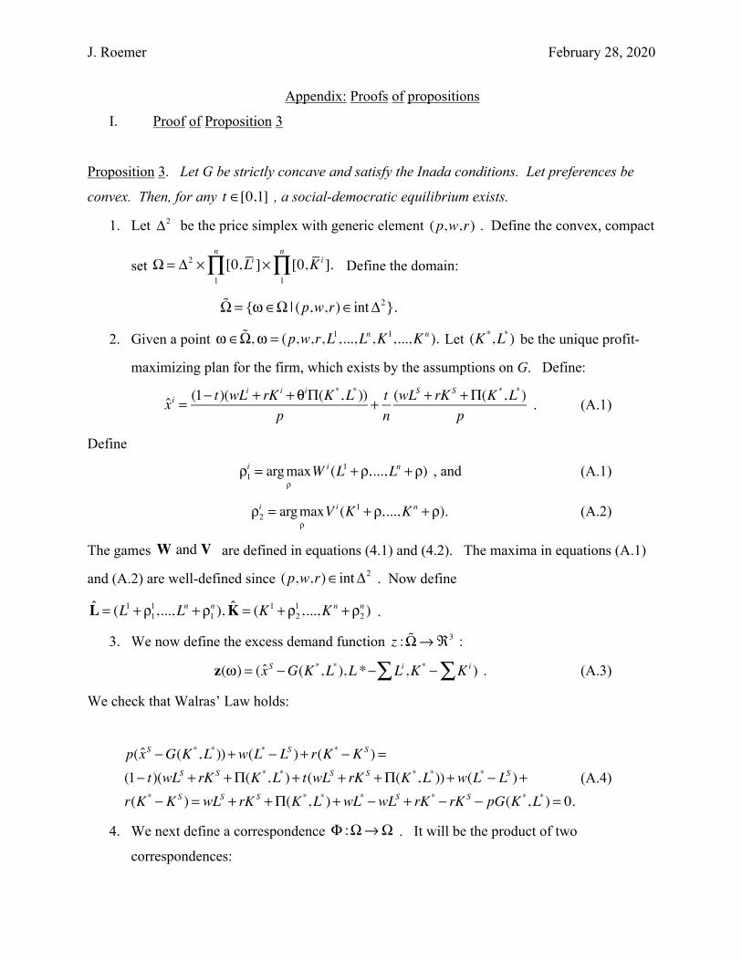
J. Roemer February 28, 2020
Appendix: Proofs of propositions
I. Proof of Proposition 3
Proposition 3. Let G be strictly concave and satisfy the Inada conditions. Let preferences be
convex. Then, for any , a social-democratic equilibrium exists.
1. Let be the price simplex with generic element . Define the convex, compact
set Define the domain:
2. Given a point Let be the unique profit-
maximizing plan for the firm, which exists by the assumptions on G. Define:
. (A.1)
Define
, and (A.1)
(A.2)
The games are defined in equations (4.1) and (4.2). The maxima in equations (A.1)
and (A.2) are well-defined since . Now define
.
3. We now define the excess demand function :
. (A.3)
We check that Walras’ Law holds:
(A.4)
4. We next define a correspondence . It will be the product of two
correspondences:
t ∈[0,1]
Δ2 (p,w,r)
Ω = Δ2 × [0,Li1
n
∏ ]× [0,Ki ].1
n
∏!Ω = {ω ∈Ω | (p,w,r)∈intΔ2}.
ω ∈ !Ω,ω = (p,w,r,L1,...,Ln ,K1,...,Kn ). (K *,L*)
xi = (1− t)(wLi + rK i + θiΠ(K *,L*))
p+ tn(wLS + rK S +Π(K *,L*)
p
ρ1i = argmax
ρW i (L1 + ρ,...,Ln + ρ)
ρ2i = argmax
ρV i (K1 + ρ,...,Kn + ρ).
W and V
(p,w,r)∈intΔ2
L = (L1 + ρ11,...,Ln + ρ1
n ), K = (K1 + ρ21 ,...,Kn + ρ2
n )
z : !Ω→ℜ3
z(ω) = (xS −G(K *,L*),L *− Li ,K *∑ − Ki )∑
p(xS −G(K *,L*))+w(L* − LS )+ r(K * − KS ) =(1− t)(wLS + rK S +Π(K *,L*)+ t(wLS + rK S +Π(K *,L*))+w(L* − LS )+r(K * − KS ) = wLS + rK S +Π(K *,L*)+wL* −wLS + rK * − rK S − pG(K *,L*) = 0.
Φ :Ω→Ω

2
(A.5)
Define
. (A.6)
Define
. (A.7)
5. Suppose that w is a fixed point of F. Thus, . By the definition of ,
. We have by Walras’ Law. It follows by the
definition of that the three components of are all non-positive, since otherwise
we could choose a vector rendering . But since is a
positive vector, it follows that . Therefore, all markets clear at this price
vector.
6. Finally, since w is a fixed point, we have for all i, . This proves that the
vectors L and K are indeed additive Kantian equilibria of their respective games,
.
7. This will prove the existence of equilibrium, if the conditions of Kakutani’s fixed point
theorem hold. F is convex-valued if preferences and G are concave, and it is upper-
hemi-continuous as well. This concludes the proof.+ ■
II. Proof of Proposition 5
Proposition 5 Let G be strictly concave and satisfy the Inada conditions; let preferences be
convex and let the three goods be normal goods. Then for any , a Pareto efficient -
sharing equilibrium exists.
Proof:
+ The proof technique – in particular, the definition of the correspondence -- is taken from Mas-Colell, Whinston and Green (1995).
Φ(ω) = Φ1(ω)×Φ2 (ω).
Φ1(ω) ={q∈Δ2 | (∀ ′q ∈Δ2 )(z(ω) ⋅q ≥ z(ω) ⋅ ′q )} if ω ∈ !Ω,
{q∈Δ2 | q ⋅(p,w,r) = 0} if ω ∈Ω \ !Ω
⎧⎨⎪
⎩⎪
Φ2 (ω) =(L,K) if ω ∈ !Ω,
(0,0,...,0) if ω ∈Ω \ !Ω
⎧⎨⎪
⎩⎪
(p,w,r)∈Φ1(ω) Φ1
(p,w,r)∈intΔ2 z(ω) ⋅(p,w,r) = 0
Φ1 z(ω)
′q ∈Δ2 z(ω) ⋅ ′q > 0 (p,w,r)
z(ω) = (0,0,0)
ρ1i = 0 = ρ2
i
W and V
λ ∈[0,1] λ
Φ1

3
1. We will define a correspondence on the price simplex, whose generic
element is . This step and steps 2 through 8 set up the structure that will allow
us to define in step 9. Given , by the Inada conditions and strict
concavity of G, there exists a unique vector that maximizes profits
. Denote profits at the optimum by .
2. Consider the system of equations in the unknowns :
(i)
(ii) .
(iii) .
I claim there is a unique solution to these equations where for all i, with
and .
3. To see this, we first show that there is a unique solution to the equations in statements (i)
and (ii), for any . Note that for any the two equations
in statement (i) define an expansion path that is a monotone increasing
path (MIP) in , beginning at the origin and increasing without bound. This is a MIP
by the assumption that the three goods are normal goods1.
4. Second, rewrite the equations in statement (ii) as:
(ii’) .
(A.8)
From statement (ii’), it is clear that the set of solutions to (ii’) is a
simplex (that is, a triangle whose sides lie in the three co-ordinate planes) in .
5. It is clear the MIP for consumer i defined in step 3 intersects this simplex in a unique
point. This being true for every i, we have demonstrated the claim in the first sentence of
1 As income increases, utility maximization engenders in increase in all three goods, which yields the MIP.
Φ :Δ2 →→Δ2
(p,w,r)
Φ (p,w,r)∈intΔ2
(K *,L*)
pG(K ,L)−wL − rK Π(K *,L*)
{{(xi ,Li ,Ki ) | i = 1,...,n},A,B}
(∀i) − u2i (xi ,Li ,Ki )u1i (xi ,Li ,Ki )
= wp
and − u3i (xi ,Li ,Ki )u1i (xi ,Li ,Ki )
= rp
,
(∀i) pxi = wLi + rK i + (λ Li
A+ (1− λ)K
i
B)Π(K *,L*)
A = LS and B = KS
(Li ,Ki )∈[0,Li ]× [0,Ki ] (A,B )∈(0,LS ]× (0,K S ]
(A,B)∈(0,LS ]× (0,KS ] i = 1,...,n,
(x,Li − L,Ki − K )
ℜ+3
pxi + (w + λAΠ)(Li − Li )+ (r + 1− λ
BΠ)(Ki − Ki ) = (w + Π
A)Li + (r + Π
B)Ki
(x,Li − L,Ki − K )
ℜ+3

4
step 3. Denote the solution to the equations in statements (i) and (ii) for fixed by
6. We proceed to prove the claim stated in the last sentence of step 2. To do so, we define a
function First, we define on .
For we have a unique solution satisfying statements
(i) and (ii). From this, define . Let . Next,
we define if either A or B equals 0. is clearly continuous when
is a positive vector by Berge’s theorem. It is continuous at points when either A or B is
zero because from equation (ii’), income approaches infinity as A or B approaches zero,
and so both and approach zero in the solutions . Therefore in this case
, proving continuity.
7. By Brouwer’s fixed point theorem, it follows that the continuous function possesses a
fixed point, and this is a solution to the equations (i) in step 2 and :
(ii”) .
8. We now define the excess demand correspondence on by:
.
z is a correspondence because there may be more than one fixed point of the function .
It follows from the budget constraints (ii”) that Walras’s Law holds:
on .
9. We finally define the correspondence whose fixed point will be a sharing
equilibrium. Define by:
Let be a fixed point of . It follows from the definition of that
-- its components are all positive. But Walras’s Law holds, and this
(A,B)
P(A,B).
θ :[0,LS ]× [0,KS ]→ [0,LS ]× [0,KS ]. θ (0,LS ]× (0,K S ]
(A,B)∈(0,LS ]× (0,K S ] P(A,B)
LS = Lii∑ and KS = Ki
i∑ θ(A,B) = (LS ,KS )
θ(A,B) = (0,0) θ (A,B)
Li Ki P(A,B)
(LS ,KS )→ (0,0)
θ
(∀i) pxi = wLi + rK i + (λ Li
LS+ (1− λ) K
i
K S )Π(K*,L*)
intΔ2
z(p,w,r) = (xS −G(K *,L*),L* − LS ,K * − KS )
θ
z(p,w,r) ⋅(p,w,r) = 0
intΔ2
λ −
Φ :Δ2 →→Δ2
Φ(p,w,r) ={q∈Δ2 | (∀ ′q ∈Δ2 )(z(p,w,r) ⋅q ≥ z(p,w,r) ⋅ ′q )} if (p,w,r)∈intΔ2
{q∈Δ2 | q ⋅(p,w,r) = 0} if (p,w,r)∈∂Δ2
⎧⎨⎪
⎩⎪
(p,w,r) Φ Φ
(p,w,r)∈intΔ2

5
implies by the definition of that has no positive component. But then,
invoking Walras’s Law again, it follows that , and so all markets
clear at this allocation.
10. We must show that the vectors associated with the fixed point
are multiplicative Kantian equilibria of their respective games R and I, which are defined
in equations (5.1) and (5.2). The conditions that this be so are:
(a) for all i, , and
(b) for all i, (ii”) holds.
Observe that if and are positive, then condition (a) is equivalent to condition (i),
and if or is zero, then condition (a) holds automatically. Therefore, the
conditions that the two supply vectors be multiplicative Kantian equilibria of the games
hold.
11. The allocation is Pareto efficient by condition (i) and profit-maximization, which imply
that all marginal rates of substitution equal the relevant marginal rates of transformation.
12. It finally remains to show that the correspondence is convex-valued and upper-hemi-
continuous. This follows from the premises of the proposition. ■
III. Proof of Proposition 9
Proposition 9 Let be consumer i’s consumption, supply of labor to
the private and public good firms, respectively, and her supply of capital to the
private and public good firms, respectively. Let z be the level of the public good. An
interior allocation is Pareto efficient if and only if:2
2
Φ z(p,w,r)
z(p,w,r) = (0,0,0)
(L1,...,Ln ) and (K1,...,Kn )
(u1i wp+ u2
i )Li = 0, (u1i rp+ u3
i )Ki = 0
Li Ki
Li Ki
R and I
Φ
(xi ,L1i ,L2
i ,K1i ,K2
i )
(i)(− u2i
u1i = G2 ), (ii)(∀i)(−
u3i
u1i = G1) (iii) u4
i
u2i
i∑ = − 1
H2
, and (iv) u4i
u3i
i∑ = − 1
H1
.

6
(A.15)
1. Pareto efficiency for an allocation in the model of Definition 7 is characterized by the
KKT conditions of the following program:
(A.16)
2. For convenience, let Then the KKT conditions of this program are:
3. After eliminating the unknown Lagrangian multipliers from this system of
equations, we end up with precisely conditions (i) – (iv) stated in Proposition 9. These
conditions, plus the conditions given by the primal constraints in (A.16), which are all
binding, characterize Pareto efficiency. ∎
maxu1(x1,L1,K1, z)subj. to (∀i >1) ui (xi ,Li ,Ki , z) ≥ ki (λi )xS ≤G(K1,L1) (α)z ≤ H (K2,L2 ) (β)K1 + K2 ≤ K
S (γ )L1 + L2 ≤ L
S (δ)
λ1 = 1.(∂xi ) for all i : λiu1
i = α
(∂Li ) for all i : λiu2i + δ = 0
(∂Ki ) for all i : λiu3i + γ = 0
(∂L1)αG2 = δ(∂L2 )βH2 = δ(∂K1)αG1 = γ(∂K2 )βH1 = γ
(∂z) λ ju4j
j=1
n
∑ = β
n + 3