HAL Id: jpa-00210181https://hal.archives-ouvertes.fr/jpa-00210181

Submitted on 1 Jan 1986

HAL is a multi-disciplinary open accessarchive for the deposit and dissemination of sci-entific research documents, whether they are pub-lished or not. The documents may come fromteaching and research institutions in France orabroad, or from public or private research centers.

L’archive ouverte pluridisciplinaire HAL, estdestinée au dépôt et à la diffusion de documentsscientifiques de niveau recherche, publiés ou non,émanant des établissements d’enseignement et derecherche français ou étrangers, des laboratoirespublics ou privés.

Marangoni convection induced by a nonlineartemperature-dependent surface tension

A. Cloot, G. Lebon

To cite this version:A. Cloot, G. Lebon. Marangoni convection induced by a nonlinear temperature-dependent surface ten-sion. Journal de Physique, 1986, 47 (1), pp.23-29. �10.1051/jphys:0198600470102300�. �jpa-00210181�

23

Marangoni convection induced by a nonlinear temperature-dependentsurface tension

A. Cloot and G. Lebon

Liège University, Thermodynamique des Phénomènes Irréversibles,B5, Sart Tilman, 4000 Liège, Belgium

(Reçu le 13 mai 1985, revisé le 29 août, accepté le 19 septembre 1985)

Résumé. 2014 On étudie l’instabilité de Marangoni dans une mince lame horizontale de fluide lorsque la tensionde surface est une fonction non linéaire de la température. Un tel comportement est typique de solutions aqueusesd’alcools à longue chaîne. La zone des solutions stationnaires convectives est déterminée en fonction du nombred’onde et d’un nouveau nombre sans dimension, le nombre de Marangoni du second ordre. On montre que lescellules prenant la forme de rouleaux et de rectangles sont instables alors que les hexagones sont stables. Leséquations de champ sont exprimées sous forme d’équations d’Euler-Lagrange d’un principe variationnel quiconstitue le point de départ de la procédure numérique, basée sur la méthode de Rayleigh-Ritz.

Abstract 2014 Marangoni instability in a thin horizontal fluid layer exhibiting a nonlinear dependence of the surface-tension with respect to the temperature is studied. This behaviour is typical of some aqueous long chain alcoholsolutions. The band of allowed steady convective solutions is determined as a function of the wavenumber and anew dimensionless number, called the second order Marangoni number. We show that the cells which take theshape of rolls and rectangles are unstable while hexagonal planforms remain allowed The field equations areexpressed as Euler-Lagrange equations of a variational principle which serves as the starting point of the nume-rical procedure, based on the Rayleigh-Ritz method.

J. Physique 47 (1986) 23-29 JANVIER 1986,

Classification -

Physics Abstracts47.25Q

1. Introduction.

In most papers on Marangoni instability, the surface-tension is supposed to be a monotonically linearlydecreasing function of temperature [1-4]. Thisbehaviour is typical of a large class of fluids like water,silicone oil, water-benzene solutions, etc. In excep-tional cases, one may find systems like some alloys,molten salts or liquid crystals with a surface-tensiongrowing linearly with temperature [5-7]. There existshowever a third class of fluid systems characterizedby a surface-tension exhibiting a nonlinear dependencewith respect to temperature and passing through aminimum (see Fig. 1). This behaviour is representativeof aqueous long chain alcohol solutions and somebinary metallic alloys [8-9].

The purpose of this paper is to study the effect of anonlinear temperature dependence of the surface-tension on the convective motion observed in a thinhorizontal fluid layer subject to heating (Marangoniproblem). Buoyancy forces are neglected, which is areasonable hypothesis in a microgravity environment(10- 6 g to 10- 3 g).

Our analysis departs from previous works in tworespects. First, it is out of question to treat the problemwithin the linear normal mode technique. Second, theclassical Marangoni number which measures thelinear variation of the surface-tension with tempera-ture is meaningless; it is replaced by a new dimen-sionless quantity expressing the curvature of the

surface-tension-temperature curve.The numerical treatment to be used is close to the

procedure proposed in earlier papers [3, 4]. It consistsof replacing the set of field equations by a variationalprinciple. Approximate solutions are then obtained byappealing to Rayleigh-Ritz’s technique which involvesthe construction of trial functions, selected as Tche-byshev’s polynomials.The mathematical model is presented in section 2,

with special emphasis on the boundary conditions.In section 3, steady convective solutions are derived.As it appears that the number of mathematical steadysolutions is infinite, it is necessary to determine whichones are physically admissible. This is achieved byexamining the stability of the solutions with respect toinfinitesimally small superimposed perturbations (sec-tion 4). Final comments are found in section 5.

Article published online by EDP Sciences and available at http://dx.doi.org/10.1051/jphys:0198600470102300

24

Fig. 1. - Variation of the surface-tension with temperaturefor an aqueous solution of n-heptanol at various concen-trations [9]. 1 : pure water; 2 : 8 x 10-4 mol/kg; 3 :1 x 10- 3 mol/kg; 4 : 1.3 x 10- 3 mol/kg; 5 : 2 x 10 - 3 mol/kg; 6 : 5 x 10-3 mol/kg; 7 : 7.6 x 10-3 mol/kg.

2. The mathematical modeL

The system consists of a thin horizontal fluid layer ofthickness d, extending laterally to infinity and subjectto a temperature gradient. The lower face is in contactwith a perfectly rigid heat conductor while the uppersurface is free, adiabatically insulated, flat and unde-formable. The surface-tension ç exerted at the upperboundary is supposed to be a quadratic function of thetemperature, with a minimum value Çm at T = Tm :

Çm and b are given positive parameters. Law (2.1) iswell representative of aqueous alcohol solutions, asobserved in figure 1 which shows the ç( T) curves for an-heptanol-water solution for various concentrations :b is of the order of 10- 6 N/m. K2 while Çm ranges from3 x 10- 2 to 7 x 10- 2 N/m.

It is also assumed that the fluid is Boussinesquianwith constant values of density p, heat diffusivity K,kinematic viscosity v, and no viscous dissipation.

Let AT be the temperature drop between the lowerand upper boundaries of the layer. In absence of

gravity effects, the velocity u(u, v, w) and temperature 0fields satisfy the following balance equations :

where

Cartesian coordinates are selected with horizontalaxes located in the lower boundary and a vertical axispointing upwards; equations (2.2) to (2.4) are writtenin non-dimensional form with the space coordinates,time, and temperature scaled by d, d2/K, AT respec-tively, Pr is the usual Prandtl number given by

The relevant boundary conditions are :

where M and f stand respectively for

For positive values of AT, f is positive, zero or negativeaccording to whether the temperature T1 at the uppersurface is larger, equal or smaller than Tm, the tem-perature at which ç is a minimum. The quantity Mis strictly positive and is called the Marangoni numberof second order : it is related to the inverse of theradius of curvature of the ç - T curve, it takes valuesbetween 100 and 1 000 for aqueous alcohols when ATis of the order of a few degrees and d about one centi-meter.

It is worth comparing (2.7) with the analogousboundary condition formulated in the classical Maran-goni problem and expressed by

Ma is the Marangoni number defined by

In contrast with (2. 10), expression (2 . 7) is no longerlinear; moreover, the central quantity ceases to bethe Marangoni number but rather M, a strictlypositive quantity whereas Ma may be either positiveor negative. When f > 1, it is a good approximationto drop all the nonlinear terms in (2.7), which reduces

25

then to (2. 10) upon writing

On the other hand, for small values of f, which meansthat T1 is close to Tm, the nonlinearity is dominant.

3. Search for steady-state solutions.

Our objective is to determine the steady solutions of theeigenvalue problem set up by equations (2.2) to (2.7).Since it is desired to focus on the boundary effects,we shall here neglect the nonlinear terms u Vu andu V0 appearing in (2. 3) and (2. 4) : the validity of thisapproximation will be discussed at the end of section 5.

After eliminating the pressure, expressions (2.3) and(2.4) reduce to

where the subscript ss refers to the steady solution.The corresponding boundary conditions are still

given by (2.5)-(2.7) where all the quantities are

affected by the subscript ss.In view of the numerical solutions, it is convenient

to replace the relations (3.1), (3 . 2) and the associatedboundary conditions by the variational equation

where 6 is the usual variation symbol, and V and S,represent the volume of the convective cell and thearea of its upper boundary respectively. It is directlychecked that the Euler-Lagrange equations corres-ponding to arbitrary variations bw., and 60.. are

relations (3 .1) and (3 . 2) ; moreover the boundaryconditions (2.6b) and (2.7) are also recovered asnatural boundary conditions. It is worth noting that(3. 3) is not a classical variational principle in the sensethat some quantities like wss in the second volumeintegral and the quantities between brackets in thesurface integral are not submitted to variation. Sucha principle is generally classified as a quasi-variationalprinciple in the literature [11,12].

It must be realized that an « exact >> variational

principle cannot be formulated in relation with thepresent problem because the particular boundarycondition (2.7) renders the problem not self-adjoint.By the way, many principles pertain to the class ofquasi-variational principles [11, 12], a typical example

is Hamilton’s principle in classical mechanics whenfriction is present. Despite its quasi-variational pro-perty, one is however allowed to use the classical

Rayleigh-Ritz technique.Assume that there exist steady solutions of the form

with amplitudes W(z) ande(z), and where O(x, y)represents the planform in the horizontal plane;ø satisfies the relation

and is normalized so that

k is the wavenumber in the horizontal plane and ... > denotes the average over the horizontal plane.

Setting 0. -= D and substituting (3.4) into (3.3)leads to the following variational equation

where Q stands for [10]

It should be noticed that Q vanishes for cells taking the

shape of rolls, squares and rectangles while for hexa-gons, one has

26

The Euler-Lagrange equations corresponding to (3.7)are given by

while the natural boundary conditions are

It is easily checked that equations (3.10) to (3. 13)are obtained by replacing (3.4) in (3.1) and (3.2)and the boundary conditions (2.6) and (2.7) andmaking use of (3.5), (3.6) and (3 . 8).The set (3 .10) to (3.13), together with the essential

boundary conditions

is solved using the Rayleigh-Ritz method It consistsof expanding the unknown amplitudes W(z) and0(z) in terms of polynomial functions

where fn(z) and gn(z) are a priori selected functionsverifying the essential boundary conditions; theyare chosen as

where Tn (z) are the modified Tchebyshev polyno-mials. The constant coefficients an and bn in (3.16)are unknown quantities derived from the stationaryconditions

This numerical procedure predicts a steady solutionfor each value of Q. This means that any particularcellular pattern, like rolls, squares, hexagons,... is

mathematically admissible. However, observationsshow a tendency toward a single well defined cellularstructure. In order to determine the preferred form ofconvection, we shall examine the stability of thevarious steady solutions by superimposing infini-

tesimally small disturbances. In the next section, thestability of solutions consisting of rolls, rectanglesand hexagons is investigated; other planforms, likepentagons, octogons, etc. are not considered becauseno experimental evidence of their existence has everbeen displayed.

4. The preferred planform

The perturbations are assumed to be given by

where u’(u’, v’, w’) and 0’ are their amplitudes, a is areal parameter whose sign determines the stabilityof the steady solutions.The disturbances 0’ and u’ obey the linearized

equations

plus two similar equations for the u’, v’ components,which are of no use in the following. The boundarycondition at the upper boundary involving the second-order Marangoni number is written

To avoid costly and lengthy calculations, thePrandtl number is assumed to be infinite. This is

certainly a good approximation for highly viscousoils. Moreover from calculation and experimentalobservations, it is expected that Pr = oo is a reasonablehypothesis in the description of fluids with Pr > 5 [13].The variational equation giving back the set (4.3)

to (4.5) reads :

By analogy with the form (3.4) of the steady solu-tions, it is assumed that u’ and 0’ are separable andgiven by

with

where k’ is the wavenumber of the superimposedperturbation. The continuity equation O u’ = 0 re-quires that U’ and Y’ be expressed by

27

Substituting (4.7) to (4.10) into the variationalprinciple (4.6), one obtains

This equation holds for the arbitrary variations of the amplitudes 0’ and W’, compatible with the essentialboundary conditions

under the condition that the following Euler-Lagrange equations and natural boundary conditions are satisfied :

The quantity Q’ stands for

and describes the correlations between the super-imposed and the reference steady planforms; in

particular, Q’ vanishes when the wavenumber k’ ofthe superimposed pattern differs from the basicwavenumber k. Various values of Q’ are reported intable I.As in section 3, the unknowns W’ and 0’ are deter-

mined via the Rayleigh-Ritz procedure. This resultsin an eigenvalue problem for the parameters a, f, Q’,

M and k’. We fix two of them, namely f and Q’, andcalculate a for various values of M and k’. Recallingthat a > 0 means instability, we are able to dividethe plane M - k’ into two regions : one correspondingto stable solutions, the other to unstable ones. Wefirst examine the stability of the steady solutions whenthe superimposed disturbance has a wavenumber k’equal to the wavenumber k of the reference state.

Numerical results show that roll and rectangle patternsare characterized by a positive growth rate of thedisturbance (see the last column of Table I) : theseconfigurations are clearly unstable. In contrast, hexa-gons may be stable : in the M - k’ plane one can find

Table 1. - Values of the factor Q’.

28

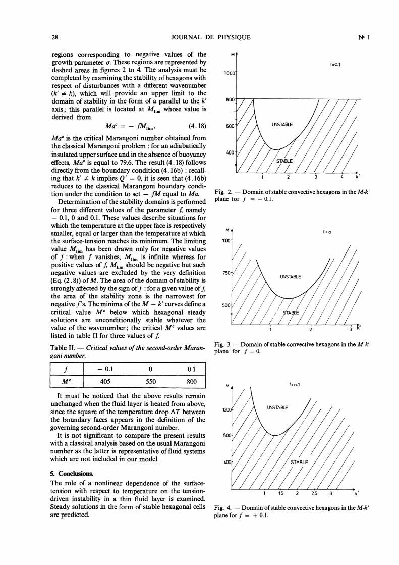
regions corresponding to negative values of the

growth parameter a. These regions are represented bydashed areas in figures 2 to 4. The analysis must becompleted by examining the stability of hexagons withrespect of disturbances with a different wavenumber

(k’ * k), which will provide an upper limit to thedomain of stability in the form of a parallel to the k’axis; this parallel is located at Mlim whose value isderived from

Mac is the critical Marangoni number obtained fromthe classical Marangoni problem : for an adiabaticallyinsulated upper surface and in the absence of buoyancyeffects, Mac is equal to 79.6. The result (4.18) followsdirectly from the boundary condition (4.16b) : recall-ing that k’ 0 k implies Q’ = 0, it is seen that (4.16b)reduces to the classical Marangoni boundary condi-tion under the condition to set - fM equal to Ma.

Determination of the stability domains is performedfor three different values of the parameter f, namely- 0.1, 0 and 0.1. These values describe situations forwhich the temperature at the upper face is respectivelysmaller, equal or larger than the temperature at whichthe surface-tension reaches its minimum. The limitingvalue Ml;m has been drawn only for negative valuesof f : when f vanishes, Mlim is infinite whereas for

positive values of f, Mlim should be negative but suchnegative values are excluded by the very definition(Eq. (2. 8)) of M. The area of the domain of stability isstrongly affected by the sign of/ : for a given value of f;the area of the stability zone is the narrowest for

negative f’s. The minima of the M - k’ curves define acritical value AC below which hexagonal steadysolutions are unconditionally stable whatever thevalue of the wavenumber; the critical Mc values arelisted in table II for three values of f.

Table II. - Critical values of the second-order Maran-goni number.

It must be noticed that the above results remain

unchanged when the fluid layer is heated from above,since the square of the temperature drop AT betweenthe boundary faces appears in the definition of thegoverning second-order Marangoni number.

It is not significant to compare the present resultswith a classical analysis based on the usual Marangoninumber as the latter is representative of fluid systemswhich are not included in our model.

5. Conclusions.

The role of a nonlinear dependence of the surface-tension with respect to temperature on the tension-driven instability in a thin fluid layer is examined.

Steady solutions in the form of stable hexagonal cellsare predicted.

Fig. 2. - Domain of stable convective hexagons in the M-k’plane for f - - U.l.

Fig. 3. - Domain of stable convective hexagons in the M-k’plane for f = 0.

Fig. 4. - Domain of stable convective hexagons in the M-k’plane for / = + 0.1.

29

The proposed model introduces several simpli-fications : gravity and non-Boussinesquian effects areignored, the Prandtl number is taken to be infiniteand the momentum and energy equations are

linearized The first approximation is reasonable in amicrogravity environment, the Boussinesq approxi-mation provides a good description for a wide classof fluids and mixtures. As discussed earlier, an infinitePrandtl number hypothesis is also readily acceptablefor viscous fluids. The validity of the approximationthat consists of linearizing the field equations ofmomentum and energy has been checked by calculat-ing the ratio between wss and the nonlinear term

uss . VOss, for different values of k and M at z = 0.5where the error is the most important. In table III,we have reported the error percentage for f = 0 :

Table III. - Error percentage in omitting the nonlinearterms in the calculation of the steady solution.

Similar orders of magnitude are obtained for non-zerof values. Although the maximum error percentageis 18 %, it falls around 5 % in the vicinity of the curveseparating the stable from the unstable convectivecells, which is undoubtly the region of interest. Itis therefore reasonable to expect that our conclu-sions should not be drastically modified by performinga fully, but costly, nonlinear analysis.

In contrast, the nonlinear contribution cannot be

neglected in the boundary condition (2.7). This

appears clearly from table IV, where the ratio of thenonlinear terms (V 16)2 + 6 Vf6 to the linear termf V’O at z = 1 is represented, for various values of theparameters.

Table IV. - Ratio between nonlinear and the linearterms at the upper surface for f = - 0.1.

Of course, a decisive check of our model can onlybe provided by experimental observations. To thisaim, in collaboration with the E.S.A. we plan to carryout some Marangoni Experiments in microgravityenvironment using such mixtures, as aqueous alcohols,whose surface-tension is a parabolic function of thetemperature.

Acknowledgments.

The authors wish to thank Professors Joos andVochten (Antwerp University) for making availablenumerical values of the surface-tension as a functionof temperature, for various alcohol aqueous solutions.

Stimulating discussions with various members ofthe FNRS Contact Group in convection, surfacetension and microgravity (Belgium) is also acknow-ledged

References

[1] PEARSON, J. R. A., J. Fluid Mech. 4 (1958) 489.[2] NIELD, D., J. Fluid Mech. 19 (1964) 341.[3] CASAS-VASQUEZ, J. and LEBON, G., Editors, Stability

of Thermodynamic Systems, Lectures Notes in

Physics, Vol.164 (Springer, Berlin) 1982.[4] CLOOT, A. and LEBON, G., J. Fluid Mech. 145 (1984) 447.[5] JOUD, J., EUSTATHOPOULOS, N., BRICARD, A. and

DESRE, P., J. Chim. Phys. 9 (1973) 1290.[6] GUYON, E. and PANTALONI, J., C.R. Hebd. Séan. Acad.

Sci. Paris 290B (1980) 301.[7] LEBON, G. and CLOOT, A., Acta Mech. 43 (1982) 141.[8] VOCHTEN, R., Ph. Thesis, University of Gent (1976).[9] VQCHTEN, R., PETRE, G. and DEFAY, R., J. Colloid Sci.

42 (1973) 310.

[10] ROBERTS, P. H., in Non-equilibrium thermodynamics,variational techniques and stability, Donnelly, Her-man, Prigogine, eds. (Chicago Univ. Press, Chi-cago) p. 125-157.

[11] FINLAYSON, B. A., The Method of Weighted Residualand Variational principles (Acad. Press, New York)1972.

[12] LEBON, G., in Recent Developments in Thermomecha-nics of Solids, Lebon and Perzyna, eds., C.I.S.M.Courses and Lectures, Vol. 262 (Springer, Wien)1980, p. 221-412.

[13] SCANLON, J. and SEGEL, L., J. Fluid Mech. 30 (1967) 149.[14] PANTALONI, J., BAILLEUX, P., SALAN, J. and VELARDE,

M., J. Non-Equilib. Thermodyn. 4 (1979) 207.