mapping u.s. forest biomass using nationwide forest ... u.s. forest biomass using nationwide forest...

Available online at www.sciencedirect.com

112 (2008) 1658–1677www.elsevier.com/locate/rse

Remote Sensing of Environment

Mapping U.S. forest biomass using nationwide forest inventory dataand moderate resolution information

J.A. Blackard a, M.V. Finco b, E.H. Helmer c, G.R. Holden d, M.L. Hoppus e, D.M. Jacobs f,A.J. Lister e, G.G. Moisen a,⁎, M.D. Nelson d, R. Riemann e, B. Ruefenacht b,

D. Salajanu f, D.L Weyermann g, K.C. Winterberger h, T.J. Brandeis f,R.L. Czaplewski i, R.E. McRoberts d, P.L. Patterson a, R.P. Tymcio a

a Rocky Mtn. Research Station, 507 25th Street, Ogden, UT 84401, United Statesb Remote Sensing Applications Center, 2200 W 2300 S, Salt Lake City, UT 84119, United States

c International Institute of Tropical Forestry, Jardín Botánico Sur, 1201 Calle Ceíba, Río Piedras, 00926, Puerto Ricod North Central Research Station, 1992 Folwell Ave, St. Paul, MN 55108, United States

e Northeastern Research Station, 11 Campus Blvd, Newtown Square, PA 19073, United Statesf Southern Research Station, 4700 Old Kingston Pike, Knoxville, TN 37919, United Statesg Pacific Northwest Research Station, 1221 SW Yamhill, Portland, OR 97205, United States

h Pacific Northwest Research Station, 3301 C St, Anchorage, AK 99503, United Statesi Rocky Mtn Research Station, 240 W Prospect Rd, Fort Collins, CO 80526, United States

Received 20 December 2005; received in revised form 24 August 2007; accepted 24 August 2007

Abstract

A spatially explicit dataset of aboveground live forest biomass was made from ground measured inventory plots for the conterminous U.S., Alaskaand Puerto Rico. The plot data are from the USDA Forest Service Forest Inventory and Analysis (FIA) program. To scale these plot data to maps, wedeveloped models relating field-measured response variables to plot attributes serving as the predictor variables. The plot attributes came fromintersecting plot coordinates with geospatial datasets. Consequently, these models serve asmappingmodels. The geospatial predictor variables includedModerate Resolution Imaging Spectrometer (MODIS)-derived image composites and percent tree cover; land cover proportions and other data from theNational Land Cover Dataset (NLCD); topographic variables; monthly and annual climate parameters; and other ancillary variables. We segmented themappingmodels for theU.S. into 65 ecologically similarmapping zones, plusAlaska and PuertoRico. First,we developed a forestmask bymodeling theforest vs. nonforest assignment of field plots as functions of the predictor layers using classification trees in See5©. Secondly, forest biomass modelswere built within the predicted forest areas using tree-based algorithms in Cubist©. To validate the models, we compared field-measured with model-predicted forest/nonforest classification and biomass from an independent test set, randomly selected from available plot data for each mapping zone.The estimated proportion of correctly classified pixels for the forest mask ranged from 0.79 in Puerto Rico to 0.94 in Alaska. For biomass, modelcorrelation coefficients ranged from a high of 0.73 in the Pacific Northwest, to a low of 0.31 in the Southern region. There was a tendency in all regionsfor these models to over-predict areas of small biomass and under-predict areas of large biomass, not capturing the full range in variability. Map-basedestimates of forest area and forest biomass compared well with traditional plot-based estimates for individual states and for four scales of spatialaggregation. Variable importance analyses revealed that MODIS-derived information could contribute more predictive power than other classes ofinformationwhen used in isolation. However, the true contribution of each variable is confounded by high correlations. Consequently, excluding any oneclass of variables resulted in only small effects on overall map accuracy. An estimate of total C pools in live forest biomass of U.S. forests, derived fromthe nationwide biomass map, also compared well with previously published estimates.© 2007 Elsevier Inc. All rights reserved.

Keywords: Forest biomass; MODIS; Classification and regression trees; Forest probability; Carbon; FIA

⁎ Corresponding author. USDA Forest Service, Rocky Mountain Research Station, 507 25th Street, Ogden, UT 84401, United States, Tel.: +1 801 625 5384; fax: +1801 625 5723.

E-mail address: [email protected] (G.G. Moisen).

0034-4257/$ - see front matter © 2007 Elsevier Inc. All rights reserved.doi:10.1016/j.rse.2007.08.021

mailto:[email protected]

http://dx.doi.org/10.1016/j.rse.2007.08.021

1659J.A. Blackard et al. / Remote Sensing of Environment 112 (2008) 1658–1677

1. Introduction

The Forest Inventory and Analysis (FIA) program of theUSDA Forest Service collects data annually on the status andtrends in forested ecosystems nationwide. These inventory datasupport estimates of forest population totals over large geographicareas, (Scott et al., 2005). Regional maps of forest characteristicswould make these extensive forest resource data more accessibleand useful to a larger and more diverse audience. Importantapplications of such maps include broad-scale mapping andassessment of wildlife habitat; documenting forest resourcesaffected by fire, fragmentation, and urbanization; identifying landsuitable for timber production; and locating areas at high risk forplant invasions, or insect or disease outbreaks. Thus, there is aneed to produce and distribute geospatial data of forest attributes,complementing FIA inventory data.

Total aboveground live biomass is a forest characteristic ofparticular interest. Forest soils and woody biomass hold most ofthe carbon in Earth's terrestrial biomes (Houghton, 1999). Land-use change, mainly forest burning, harvest, or clearing foragriculture, may compose 15 to 40% of annual human-causedemissions of carbon to the atmosphere, and terrestrial ecosystems,mainly through forest growth and expansion, absorb nearly asmuch carbon annually. However, estimates of land-atmospherecarbon fluxes, and the net of expected future ones, have thelargest uncertainties in the global atmospheric carbon budget,which adds to uncertainties about future levels and impacts ofgreenhouse gasses (GHGs) in the atmosphere (Houghton, 2003;Prentice et al., 2001).

Consequently, the levels, mechanisms and spatial distributionof forest land-atmosphere C fluxes are an important focus forreducing uncertainties in the global C budget (Fan et al., 1998;Holland et al., 1999; Pacala et al., 2001; Schimel et al., 2001).Ecosystem process models that are physiologically-based, andthat use satellite image-derived indices of photosynthesis, havepermitted unprecedented global assessments of ecosystem pro-ductivity and carbon sinks at a spatial resolution of 0.5° (Nemaniet al., 2003; Potter et al., 2003). The mechanistic nature of thesemodels identifies how observed patterns in ecosystem produc-tivity may relate to climate and atmospheric changes (Nemaniet al., 2003). However, validating atmospheric and ecosystemmodel estimates of net forest C fluxes, and quantifying the Cfluxes associated with changes in land use, which dominate thesefluxes over longer time periods, requires spatially extensive dataon forest C pools and net fluxes. Maps of forest biomass permitspatially explicit estimates of forest carbon storage and net fluxesfrom land-use change.

Our objectives here are to 1) produce a spatially explicitdataset of aboveground live forest biomass from groundmeasured inventory plots, at a 250-m cell size, for theconterminous U.S., Alaska and Puerto Rico; 2) evaluate modelperformance and spatially depict uncertainty in the dataset; 3)explore the relative contribution of the many predictor layers tothe biomass models; and 4) use the resulting dataset to estimateaboveground live forest biomass and implied carbon storage forthis area. We also describe a national geospatial predictordatabase that supported the mapping and how we standardized

national FIA data, developed predictive models, and assessedmodel error.

2. Methods

2.1. Data

2.1.1. Response variablesThe US Forest Service FIA program inventories the Nation's

forests via a network of ground-based inventory plots in whichforest structure and tree species composition are measured toproduce estimates of forest attributes like basal area by species,total volume, and total biomass. Plots are located with an intensityof about one plot per 2400 ha. Although the program historicallycollected data periodically (every 5 to 20 years) for each state inthe country, it recently shifted to an annual rotating panel system.This new system samples 10 to 20% of each state's plot networkannually (Bechtold & Patterson, 2005). This study used a mixtureof annual and historic periodic data to ensure enough trainingplots in all parts of the country, with dates of collection rangingbetween 1990 and 2003. The advantages of modeling responsevariables collected from a probabilistic sample (such as FIA's plotnetwork) over those collected from a purposive sample areexplored in Edwards et al. (2006).

The FIA program observes, measures, and predicts manyforest attributes on each plot (Miles et al., 2001). This nationwidebiomass mapping effort modeled two of these plot-level responsevariables: a binary forest/nonforest classification and above-ground live forest biomass. According to FIA definitions, forestland is at least 0.405 ha in size, has a minimum continuouscanopy width of 36.58 m with at least 10% stocking, and has anunderstory undisturbed by a nonforest land use like residences oragriculture. Aboveground live biomass includes biomass in livetree bole wood, stumps, branches and twigs for trees 2.54-cmdiameter or larger and is derived from region- or species-specificallometric equations.

2.1.2. National geospatial predictor layersA nationwide geospatial dataset of layers of predictor

variables, also called the national geospatial predictor layerdatabase, was assembled for use in the biomass models. The datalayers included satellite imagery and predicted land-cover fromModerate Resolution Imaging Spectro-radiometer (MODIS)(Justice et al., 2002), Landsat Thematic Mapper image-derivedNational Land Cover Dataset (NLCD92, Vogelmann et al., 2001),raster climate data, and topographic variables. Datasets withnative spatial resolutions other than 250 m were resampled with anearest neighbor procedure if categorical, and a bilinearinterpolation procedure if continuous. The 250-m spatialresolution of the predictor dataset has two origins. First, thecoarser spatial scale of MODIS would be practical given thenational extent of the project, and the MODIS sensor bands 1 and2 are available at that spatial resolution. As a result, MODISvegetation index data are available with 250-m pixel sizes.Secondly, we expected that coarser image data would havescaling advantages when working with passive optical imagery,as we discuss later.

1660 J.A. Blackard et al. / Remote Sensing of Environment 112 (2008) 1658–1677

Data from MODIS for the year 2001 included all land surfacereflectance bands (Vermote & Vermueulen, 1999) (MOD 09v003)from three 8-day image composites at 500-m resolution (be-ginning Julian days 097, 225, 321), three 16-day vegetation index(VI) composites (Huete et al., 2002) (MOD 13v003) at 250-mresolution over the same three compositing periods, and percenttree cover (MOD 44) at 500-m resolution for 2001 (Hansen et al.,2003). The compositing periods represented early, peak, and leaf-off phenological conditions in the continental United States. ForPuerto Rico, persistent cloudiness necessitated data from dry-season MODIS image compositing periods, including six periodsfrom 2001–2003. The MOD 09 8-day image composites use aminimum-blue criterion to select for clearest conditions (Vermote& Vermueulen, 1999). The compositing algorithm for MOD 13VI data first selects clear pixels over the compositing period withthe MODIS cloud mask. A pixel-level fit to a bidirectionalreflectance distribution function (BRDF) then estimates a near-nadir reflectance for each band for calculating VI values. If fewerthan five pixels are clear over the compositing period, then thealgorithm selects a clear pixel based on viewing angle. Otherwise,the algorithm selects the pixel with the maximum NormalizedDifference Vegetation Index (NDVI) (Huete et al., 2002). Weperformed no additional image compositing or cloud filling forcontinental U.S. imagery. Some cloudy areas were masked fromthe Puerto Rico composites and filled with appropriate compositeimagery from other dates.

Landsat image-based land cover for the conterminous U.S.(Vogelmann et al., 2001) and Puerto Rico (Helmer et al., 2002)provided data on proportional cover of forest, shrubland, wetlandand urban/barren lands (Puerto Rico only). These 30-mcomponents of the national geospatial predictor data used focalfunctions to summarize the land cover class proportions within a9×9 moving window and subsequently resampled the data to250-m with bilinear resampling. Climate data included 30-year(1961–1990) average monthly and annual precipitation andtemperature measures, represented by spatial resolutions of about4 km for the conterminous U.S. (Daly et al., 2000), 2 km forAlaska (Daly, 2002) and 420-m for Puerto Rico (Daly et al.,2003). The dataset also included elevation from 30-m digitalelevation models (DEMs) (Gesch et al., 2002), and othertopographic derivatives from those DEMs, including slope,dominant aspect, and an indicator of aspect variety. This indicatoris calculated as the total number of unique aspect values (or thevariety) within the nine by nine window surrounding each 30-mcell. The resulting dataset was resampled to a 250-m cell size. Thesame resampling method used for the 30-m Landsat products(described above) was used to summarize the elevation-basedattributes at 250-m. A final topographic variable that severalmodels used was a horizontal-distance-to-nearest-stream mea-sure, which is the Euclidean distance from each pixel to its nearestabove-ground water body, as the crow flies.

2.2. Modeling strategy

2.2.1. Process overviewWe created a nationwide modeling dataset by intersecting plot

locations with the geospatial predictor layers, and extracting all

relevant data. Resulting values of predictor layers for each plotwere then linked to the corresponding forest/nonforest and forestbiomass response variables. We segmented this modeling datasetinto 65 ecologically unique mapping/modeling zones (Fig. 1)(Homer & Gallant, 2001) which permitted separate models totarget the conditions unique to each zone. However, weaggregated adjacent zones in sparsely forested regions, whichhad too few forested plots, to increase the number of observationsin the models for those zones. Independent test sets were createdby randomly selecting 10 to 15% of the plots by mapping zone,leading to proportional distribution by zone. These test sets werewithheld to assess model performance, except in Puerto Ricowhere insufficient numbers of plots forced the use of 10-foldcrossvalidation for evaluating biomass model performance. Usingclassification trees with boosting for each mapping zone, we firstproduced a 250-m resolution forest mask by modeling the binaryvariable of forest/nonforest as a function of all the variablescontained in the national geospatial predictor layers. We thenselected only those FIA plots that fell within the forested portionof the forest mask as training data for the biomass models.Regression tree algorithms were then used to model forestbiomass (also at 250 m) as a function of those same predictorvariables used in the forest/nonforest models for each mappingzone. Because of ecological differences between zones, the wayin which the classification trees used and partitioned the predictorvariables was very different by zone. Also, some regionalvariations in the methods themselves were used to improve theforest/nonforest and biomass models. Examples include inclusionof regional specific predictor layers and larger groupings ofsimilar mapping zones. We then predicted forest biomass on aper-pixel basis by applying the models developed for eachmapping zone to the corresponding predictor layers for that zone.Pixels with nonforest class label predictions were omitted fromsubsequent analyses, and labeled as having no forest biomass.Finally, using the classification confidence and absolute errorinformation available from the models, two additional geospatialdatasets were created to capture the per-pixel uncertaintyassociated with each estimate – resulting in a map of forestprobability, and a map of biomass percent error (details in sectionon Uncertainty maps). The individual zone maps of forest/nonforest, forest probability, biomass, and percent errorfor biomass were mosaiced to form nationwide datasets. Astate boundary geospatial layer identified coastal shorelines(nationalatlas.gov/statesm.html), and a national hydrographylayer (nationalatlas.gov/hydrom.html) delineated interior waterboundaries.

2.2.2. Classification and regression treesClassification and regression tree modeling, or recursive

partitioning regression (Breiman et al., 1984), is available inmany software packages and is now common in remote sensingapplications. To give a general overview of the methodology,trees subdivide the space spanned by the predictor variables intoregions for which the values of the response variable are mostsimilar, and then assign a unique prediction for each of theseregions. The tree is called a classification tree if the responsevariable is discrete and a regression tree if the response variable is

http://nationalatlas.gov/statesm.html

http://nationalatlas.gov/hydrom.html

Fig. 1. Mapping/modeling zones (Homer & Gallant, 2001) segmented forest vs. nonforest and biomass classification and mapping models.


continuous. Tree-based methods have evolved to enhance theirpredictive capabilities. Two recent enhancements have hadconsiderable success in mapping applications (Chan et al.,2001). One is known as bagging, or bootstrap aggregation (Bauer& Kohavi, 1998; Breiman, 1996). The other is called boosting(Freund & Schapire, 1996) with its variant Resampling andCombining (ARCing) (Breiman, 1998). These iterative themeseach produce a committee of expert trees by resampling withreplacement from the initial data set, then averaging the treeswith a plurality voting scheme if the response is discrete, orsimple averaging if the response is continuous. The differencebetween bagging and boosting is the type of data resampling. Inbagging, all observations have equal probability of entering thenext bootstrap sample. In boosting, problematic observations,those which are frequently misclassified, have a higher prob-ability of selection. The performance of tree-based methods formodeling FIA response variables is compared to other modelingtechniques in Moisen and Frescino (2002) and Moisen et al.(2006).

Specifically for this study, classification trees with boosting (5or 10 trials) and pruning in See5 (www.rulequest.com, Quinlan,1986, 1993) generated the forest mask based on a 0.5 thresholdfor distinguishing forest from nonforest. Cubist (www.rulequest.com) generated the mapping models of forest biomass withinpixels predicted to be forested. Cubist is a proprietary variant onregression trees with piecewise nonoverlapping regression.Specific software options used for most mapping zones included

the following: either 5 or 10 committee models; use of rules alone(no instances); minimum rule cover of 1% of cases; extrapolationup to 10%; and no maximum number of rules.

2.3. Model performance

Measures for assessing and depicting accuracies, errors, anduncertainties of the modeled spatial datasets were chosen bytaking into consideration traditional methods of accuracyassessment, known characteristics of the datasets, and theiranticipated uses.

2.3.1. Per-pixel measuresAccuracy and error measures for the forest mask included

proportion of correctly classified units (PCC), Kappa (Cohen,1960), as well as omission and commission errors for boththe forest and nonforest classes. PCC is a statistic that canbe deceptively high when the proportion of a class, in thiscase forest, is very low or very high. The Kappa statisticmeasures the proportion of correctly classified units afterremoving the probability of chance agreement. Errors ofomission (1-producer's accuracy) result when a pixel isincorrectly classified into another category, thus being omittedfrom its correct class. Errors of commission (1-user's accuracy)result when a pixel is committed to an incorrect class. For thebiomass map, the per-pixel accuracy measures that we calculatedon the independent test sets included average absolute error,

http://www.rulequest.com




relative error, and correlation. The average absolute error for aset of test cases is the average of the sizes of differences betweenthe actual and predicted values for each case, expressed in metrictons per ha. The relative error is the ratio of the average absoluteerror to the average absolute error that would result bypredicting the value of each case as the mean of the trainingset. Because it is normalized by the predicted value's unit ofmeasure, the relative error term is useful for comparing theperformance of different models. It also gives an indication ofindividual model performance above and beyond simply usingthe average value from the training data as its ‘predicted’ value.A relative error substantially less than one indicates that themodel predictions are substantially better than simply using aprediction of the sample mean. The correlation coefficient is astandard measure of the linear relationship between observedand predicted values.

2.3.2. Uncertainty mapsOne of the goals of this study was to provide spatially explicit

depictions of the uncertainty in both the forest mask and forestbiomass maps. Maps of uncertainty are derived from themodeling process itself and provide users (and developers)information on where the model was more and less confident ofthe estimate based on the training and predictor informationavailable and the modeling technique used.

For the forest/nonforest map, a binary response variable, theneed for a spatial depiction of uncertainty was satisfied with aforest probability dataset, depicting the probability that anyindividual pixel could be classified as forest. In many modelingapplications for binary response variables, predictions are madeon a continuum of 0 to 1, indicating probability of a pixelbelonging to the class of interest. Because of the way in whichSee5 constructs predictions, a map of forest probability had to beback-engineered in the following way. First, the public C codedistributed with See5 (http://rulequest.com/see5-public.zip) en-abled us to produce a confidence value for each pixel predictionas a forest/nonforest classification confidence map. This softwareroutine operates as follows: if a single classification tree is usedand a case is classified by a single leaf of a decision tree, theconfidence value assigned is the proportion of training cases atthat terminal node that belongs to the predicted class. If more thanone terminal node is involved, the confidence value assigned is aweighted sum of the individual nodes' confidences. If more thanone tree is involved (eg. boosting), the value is a weighted sum ofthe individual trees' confidences. Second, a forest probabilitymap was created by remapping confidence values from the public

Table 1Per-pixel measures of performance for forest/nonforest maps based on independent

Region PCC Kappa Omission forest Commission fores

Northeast 0.89 0.77 0.08 0.09Northcentral 0.93 0.80 0.15 0.15Interior West 0.91 0.76 0.17 0.18Pacific Northwest 0.85 0.61 0.05 0.15Southern 0.86 0.69 0.10 0.13Alaska 0.94 0.88 0.07 0.08Puerto Rico 0.79 0.57 0.07 0.28

C code to a range of 0 to 0.5 for nonforest pixels and 0.5 to 1 forforest pixels, creating a new range from 0 to 1. Here, values near 0indicate a more confident prediction for nonforest areas, valuesnear 1.0 indicate a more confident prediction for forest areas, andvalues around 0.55 are the most uncertain.

For the map of aboveground forest biomass, spatial depictionsof uncertainty took the form of biomass percent error maps. Thesewere derived by first extracting the weighted average absoluteerror of all the rules that applied to each pixel, in which theaverage absolute error for each rule is from the training data. Thebiomass percent error map then resulted from dividing thatweighted average absolute error by the predicted biomass value atthat pixel. Such uncertainty maps provide information regardingboth the location and magnitude of potential errors in the modeledestimates. They allow users to incorporate this information intoall further modeling or analysis efforts using the estimatedbiomass and forestland maps/datasets (Fortin et al., 1999;Mowrer, 1994; Woodbury et al., 1998).

2.3.3. Agreement of spatial aggregationsFIA plot data is typically used to produce unbiased estimates

of forest population totals using design-based inference(Cochran, 1977; Särdnal et al., 1992; Thompson, 1997) forareas of sufficient size. Often in practice, however, maps may beused to produce population estimates of these mapped variablesby summing pixels over the geographic area of interest. Thismethod relies on model-based inference (Valliant et al., 2001).To provide information on the comparative accuracy of these“map-based” estimates of area of forestland and total biomass,we compared them to “plot-based” estimates of total forest areaand biomass by state for the US using FIA sample plots (Scottet al, 2005). Note that although FIA will use remote sensinginformation to stratify sample plots to improve precision inestimates of forest population totals, the plot-based estimatesused here are solely based on field data. This comparison allowsusers of inventory data who are familiar with the traditional plot-based estimates to examine the location and magnitude of areasof over-and underestimation of map-based estimates.

Next, in order to examine the scales at which aggregatedestimates of forest area or total forest biomass agree with plot-based estimates, we also made comparisons for hexagons at fourdifferent sizes: ∼16,000, ∼21,000, ∼39,000, and ∼65,000 ha.The hexagons were derived by tessellation from the Environ-mental Monitoring and Assessment Program hexagons (Whiteet al., 1992) that are used as the basis for the FIA sampling design(Bechtold & Patterson, 2005). For both area of forestland and

test sets, reported by region

t Omission nonforest Commission nonforest Test set sample size

0.14 0.14 11810.05 0.05 54490.07 0.06 71960.39 0.15 25880.22 0.17 31380.05 0.04 65530.36 0.10 28

http://rulequest.com/see5-public.zip

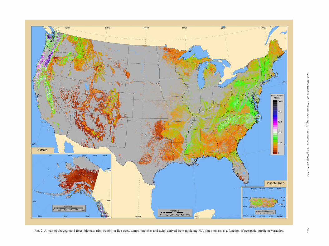
Fig. 2. A map of aboveground forest biomass (dry weight) in live trees, tumps, branches and twigs derived from modeling FIA plot biomass as a function of geospatial predictor variables.

1663J.A

.Blackard

etal.

/Rem

oteSensing

ofEnvironm

ent112

(2008)1658–1677

Table 2Per-pixel measures of performance for biomass maps based on independent testsets (except for Puerto Rico where 10-fold cross-validation was used), reportedby region

Region Average absoluteerror

Relativeerror

Correlation Test set samplesize

Northeast 60.1 0.89 0.39 1156Northcentral 42.5 0.88 0.46 1134Interior West 42.2 0.65 0.66 2023PacificNorthwest

163.1 0.72 0.73 1591

Southern 60.2 0.92 0.31 1939Alaska 91.5 0.59 0.69 430Puerto Rico 65.0 0.51 0.92 ⁎

⁎Based on a 10-fold cross validation.Average absolute error is reported in metric tons per hectare.


aboveground forest biomass, agreement between the mean ofpixel predictions for all pixels with centers in a hexagon to themean of plot observations for all plots with centers in the hexagonwas assessed as follows. For each hexagon, the mean pixelprediction, μ̂pixel, for a hexagon was compared to the plot-basedmean, μ̂plot, using,

s ¼ l̂pixel �l̂plotSE l̂plot

� �

where SE(μ̂plot) denotes the design-based standard error. Here, τis not a formal statistic with an established distribution andprobability levels. Rather it is constructed as a heuristic tool bywith which to assess relative agreement between traditional plot-based estimates, and map-based estimates at varying scales ofaggregation.

Arrays of hexagons of four sizes were considered:∼16,000 ha, ∼21,000 ha, ∼39,000 ha, and ∼65,000 ha. Basedon a sampling intensity of approximately one plot per 2400 ha,hexagons of ∼16,000 ha would include 6–7 plots, about thesmallest sample sizes that would yield reliable estimates of SE(μ̂plot). Selection of the sizes of the larger hexagons was arbitrary,except for the ∼65,000-ha EMAP hexagons, from which uniqueID codes are attributed to FIA plots and which are used in severalnational assessments. For areas of the country in which acomplete cycle of sampling has not been completed, somehexagons may include fewer than 6–7 plots. No comparisons ofpixel-and plot-based means were calculated for hexagons withfewer than 5 plots. Tau-values exceeding 2 were interpreted as aconservative indication that model-based estimates disagreedwith plot-based estimates within each hexagon.

2.3.4. Variable importanceA series of variable importance analyses were conducted to

assess the relative contributions of the numerous predictorvariables to the modeling process. First, the relative importanceof the major groups of predictor variables were assessed in eachregion. This was measured by percent improvement, or decrease,in relative error when each major group was used alone aspredictor sets in different models of biomass. Major groups were

the “MODIS group” (including NDVI, Enhanced VegetationIndex [EVI], spectral bands, fire, and percent tree cover), the“Climate group” (including all precipitation variables), the“NLCD group” (including only NLCD-derived variables), andthe “Topo group” (including topographic variables). Note that inAlaska and in Puerto Rico, no NLCD data were available,and surrogate variables labeled as the “Veg group” were usedinstead.

Next, the relative importance of sub-groups of the “MODISgroup” were measured by percent improvement, or decrease, inrelative error when each of these sub-groups was used exclusivelyin the models. These sub-groups were the “Bands sub-group”(including all MODIS bands, all dates), the “NDVI sub-group”(including al NDVI variables), “Treecov sub-group” (includingpercent tree cover), the “EVI sub-group” (including all EVIvariables), and the “Fire sub-group” (including all fire-relatedvariables).

Because the true contribution of each variable to the finalbiomass map is confounded by high correlation betweenvariables, variable groups were excluded in turn from the originalbiomass model, and the effect on relative error examined. Inaddition, the potential effect on pixel aggregations were exploredby examining changes in density functions of predicted valuesunder the different models excluding variable groups in turn.

2.3.5. Estimates of C poolsFinally, estimates of C pools in live forest biomass of U.S.

forests, derived from the map developed in this study, werecompared with estimates from other national studies. Estimates ofthe mass of C for live trees, stumps, branches and twigs wereobtained by summing one-half the predicted biomass for eachpixel over the conterminous U.S., and Alaska. The one-half ruleis based on Brown and Lugo (1992). Mass of C for roots wasapproximated as 20% of total predicted biomass (Cairns et al.,1997). Results were compared those obtained by Turner et al.(1995), Birdsey and Heath (1995), Potter (1999), and Dong et al.(2003).

3. Results

All maps produced in this study, including the forest/nonforestmask, forest probability, forest biomass, and biomass percenterror, are available for download via http://svinetfc4.fs.fed.us/rastergateway/biomass/.

3.1. Per pixel measures

As illustrated in Table 1, the forest mask was reasonablyaccurate in all regions, with regional PCCs ranging from 0.79in Puerto Rico to 0.94 in Alaska, and regional Kappa valuesranged from 0.57 in Puerto Rico to 0.88 in Alaska, reflectingfair to excellent class agreement. Errors of omission for forestwere generally low, ranging from 0.05 in the heavily forestedPacific Northwest to 0.17 in the more nonforested InteriorWest, while errors of commission for forest ranged from 0.08in Alaska to 0.28 in Puerto Rico. Errors of omission fornonforest ranged from 0.05 in the Northcentral region and

http://svinetfc4.fs.fed.us/rastergateway/biomass/

http://svinetfc4.fs.fed.us/rastergateway/biomass/

Fig. 3. Probability of forest, biomass, and percent error in biomass mapped over Uinta Mountains in Utah, (a, b, and c respectively). Probability of forest, biomass, andpercent error in biomass mapped for the Greater Mohawk Valley Region, New York (d, e, and f respectively).


Fig. 3 (continued ).


Fig. 4. Plot-based and map-based estimates of (a) forestland and (b) total forest biomass (dry weight), by state. States are grouped by USFS Forest Inventory andAnalysis Region. A separate Y axis is provide for the Pacific Northwest states because of the substantially different scales involved.


Alaska to 0.39 in the Pacific Northwest, while errors ofcommission for nonforest ranged from 0.04 in Alaska to 0.17in the Southern region. Per-pixel measures of performance forthe forest/nonforest maps are given for individual andaggregated zones in Appendix A.

The forest biomass map is presented in Fig. 2. The models ofaboveground live forest biomass varied by region in their abilityto predict pixel-level values (Table 2). Correlation coefficientsranged from 0.92 in Puerto Rico down to 0.31 in the Southernregion. The western regions had substantially better results thandid those in the eastern regions of the US. Relative errors ranged

Table 3Assessment of agreement between plot-and map-based estimates of forest land area

Hexagonsize (ha)

Estimate Numberofhexagons

Averageplots/hexagon

Prop

−3b

16,000 Forest area 25,512 9.40 0.0121,000 Forest area 22,327 10.73 0.0139,000 Forest area 15,993 14.99 0.0165,000 Forest area 10,439 22.96 0.0216,000 Biomass 25,512 9.40 0.0021,000 Biomass 22,327 10.73 0.0039,000 Biomass 15,993 14.99 0.0065,000 Biomass 10,439 22.96 0.00

from 0.51 in Puerto Rico to 0.92 in the Southern Region, with theformer value indicating an approximate 50% improvement overusing the sample mean from the model's training dataset, versus amore modest improvement in performance over a simple samplemean indicated by the latter value. Most individual mappingzones (75%) had relative errors less than 1.0, indicating gains inthe modeling process. However, some zones actually had arelative error greater than 1.0 indicating the models performedworse than using a simple sample mean. This was particularlytrue in zones with a high proportion of scattered forest that is hardto identify with a 250 m pixel (e.g., zones 52, 44, and 49) and/or

and total biomass over 4 scales of spatial aggregation across the continental US

ortion of hexagons

τ −3≤τb−2 −2≤τb2 2≤τb3 τN3

3 0.011 0.938 0.026 0.0124 0.012 0.931 0.030 0.0149 0.019 0.908 0.036 0.0183 0.026 0.879 0.047 0.0263 0.007 0.887 0.042 0.0614 0.008 0.879 0.046 0.0635 0.012 0.860 0.049 0.0748 0.019 0.835 0.051 0.087

Fig. 5. Relative importance of the major groups of predictor variables as well as sub-groups of MODIS variables in each region. Importance is measured as the percentimprovement in relative error when each variable group is used individually in a model of forest biomass. Regional abbreviations include: AK - Alaska, IW - InteriorWest, PNW - Pacific Northwest, NC - North Central, SO - Southern, NE - Northeast, and PR - Puerto Rico.


areas missing forest data (e.g., zones 32 and 35). Biomass modelperformance results are given for individual and aggregated zonesin Appendix A.

3.2. Uncertainty maps

The forest probability map reflects uncertainty in pixelassignments to forest or nonforest categories in the forest mask.The forest probability map is a useful product of the forest-nonforest modeling process because it allows users to choosetheir own application-specific threshold for distinguishingbetween forested and nonforest lands. The biomass percenterror map reflects uncertainty in the modeled pixel-level biomassvalues.

In general, the uncertainty maps reflect those areas that aremore difficult to model because of their spatial characteristics,because of poor quality training or predictor data available inthose areas, or because of a poor relationship between thedesired response variable and the predictor layers available. Inthe forest probability map these were the interface areas betweenforest and nonforest, and in the forest biomass map these werethe areas that were less intensely sampled, more affected by landuse history (which was not an available predictor layer) orotherwise difficult to model.

Looking more closely at the resulting biomass, biomass un-certainty, and forest probability maps, regional differences inpatterns of map uncertainty are apparent. In Fig. 3a, the UintaMountains of the Interior West, large areas of highly certain

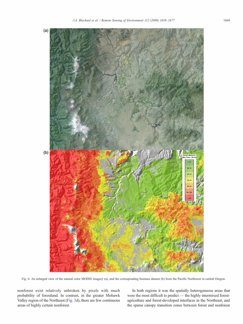
Fig. 6. An enlarged view of the natural color MODIS imagery (a), and the corresponding biomass dataset (b) from the Pacific Northwest in central Oregon.


nonforest exist relatively unbroken by pixels with muchprobability of forestland. In contrast, in the greater MohawkValley region of the Northeast (Fig. 3d), there are few continuousareas of highly certain nonforest.

In both regions it was the spatially heterogeneous areas thatwere the most difficult to predict— the highly intermixed forest-agriculture and forest-developed interfaces in the Northeast, andthe sparse canopy transition zones between forest and nonforest

Table 4Effect of excluding variable groups on relative error by region

Variablegroupsexcluded

Increase in relative error

NE NC SO INT PNW AK PR

MODIS 0.01 0.04 0.03 0.02 0.05 0.03 0.02Topo 0.00 0.00 0.01 0.01 0.01 0.02 −0.03NLCD/Veg† 0.00 0.00 0.01 0.01 0.02 0.01 0.02Climate 0.00 0.00 0.01 0.00 0.01 0.03 0.00Soils/geology – 0.01 0.01 – 0.02 – 0.00Ecozone 0.00 0.01 0.01 – 0.01 0.01 −0.02Human 0.00 – – – – – 0.00

†Land cover data for Puerto Rico from Helmer et al. (2002).Increase in relative error is measured as the difference between relative errorobtained excluding each of the major predictor groups in turn, and the relativeerror obtained using all the predictor variables.

Fig. 7. The density function in the Interior West of observed biomass values(solid line), as compared to that from a model containing all the predictorvariables (dashed line), and from a model excluding all the MODIS-derivedvariables (dotted line).


areas at the elevational (i.e. treeline) and arid limits of tree growthin the Interior West. In both regions, the probability of forestvalues falling in the most uncertain range (0.4 to 0.6) representedjust over 10% of the dataset — a substantial portion, illustratingthe difficulty of accurately determining this edge, particularly atthis resolution.

The uncertainties associated with biomass predictions in theInterior West are strongly related to the amount of biomasspresent, with higher percent errors associated with the lowerbiomass values (Fig. 3b). In the Northeast, percent errors werelower in general and show a spatial pattern that differs from thebiomass predictions themselves (Fig. 3e). This pattern may reflectthe distribution of different types of forest and our ability to modelbiomass in each, but also likely is the influence of the ancillarylayers used in the modeling. Without the strong influence of asingle variable, such as elevation, biomass predictions in theNortheast relied upon different predictor layers in different areas,each with varying levels of confidence that seemed to be visuallycorrelated with these layers. Percent error values were in generalmuch higher (above 0.8) in the Interior West (Fig. 3c) than in theNortheast (Fig. 3f). This is in large part due to the relatively lowerbiomass values present in the Interior West as compared to theNortheast.

3.3. Agreement of spatial aggregations

As described in Section 2.3.3, estimates of total forest areaand biomass were computed by state from FIA sample plots.These plot-based estimates were compared to map-basedestimates of total forest area and biomass that resulted fromcounting forested pixels and summing their biomass. At the statelevel, spatial aggregation results show fairly good agreementbetween the two sources for forest area, with notable exceptionsin CO (where the map underestimates forest area) and GA, WV,NC, TX, and OK (where the map overestimates forest area).Twenty-nine of the states' map-based estimates fell within 10%of the plot-based estimates for forest area (Fig. 4a). Foraboveground forest biomass, spatial aggregation results showan overestimation of biomass in most areas, with the notableexceptions of CA, OR, and WA where the map appears to

substantially underestimate forest biomass. Substantial overesti-mation of state-level summaries appeared to occur in NC, VA,GA, AK, CA, OR, WA, and WV. Twenty one of the states' map-based estimates fell within 10% of the plot-based estimates forbiomass (Fig. 4b).

Table 3 illustrates the distribution of τ-values to assessagreement between plot-and map-based estimates of total forestarea and total biomass at four spatial scales of aggregation acrossthe continental US. Map-based estimates of forest area generallywere in agreement with plot-based estimates for all hexagonscales. However, spatial aggregations of hexagons with largeabsolute τ-values indicate that the forest mask is problematicin some portions of the Southeast; probably in parts of Maine,Wisconsin, Minnesota, Oklahoma, and along the Great Lakes;and perhaps in parts of the Pacific Coast states. These aggre-gations of hexagons with disagreeing estimates appear to beconsistent across all four hexagon scales. Not surprisingly, thebiomass map appears to exhibit more disagreement than observedfor the forest mask at each hexagon aggregation. However, mostdisagreement in the biomass map resulted from over-estimates,while disagreement in the forest mask appeared more evenlydistributed between over-estimates and under-estimates.

3.4. Variable importance

The first column in Fig. 5 depicts the relative importance of themajor groups of predictor variables in each region. This wasmeasured by percent improvement, or decrease, in relative errorwhen each of these variable groups was used alone as predictorsets in different models of biomass. The bar labeled “All Groups”illustrates the maximum decrease in relative error obtained byincluding all the predictor variables, indicating improvement overjust using the sample mean. In four of the seven regions (NC, IW,PNW, and PR), the “MODIS group” resulted in the largestimprovement in relative error. In the other three regions (NE, SO,

Table 5Estimates of C pools in live forest biomass of continental U.S. forests

Source Approach, spatial resolution, and study area addressed Forest components Forest biomass estimatesfor the U.S. (Pg C)†

Not spatially explicitTurner et al. (1995) Inventory data by forest type at State level

(1980–1990) for conterminous U.S.Live trees, stumps, roots,branches, twigs and shrubs

14.96‡

Birdsey and Heath (1995) Inventory data by forest type at State level(1980–1992) for continental U.S.

Live trees, stumps, roots,branches, twigs, shrubs and herbs

16.74

Spatially explicitPotter (1999) Satellite-image scaled physiological model at 1°

(1980s — ignores forest age structure) for the EarthLive trees, stumps, roots,branches, twigs, and leaves.

37.65

Dong et al. (2003) Inventory data at Province level scaled with satellite imagery to 8 km(1990–1995) for Northern Hemisphere temperate and boreal countries

Live trees, stumps, roots,branches, twigs and shrubs

12.48

This study Inventory data at plot level scaled with satellite imagery to 250 m(2001) for continental U.S.†

Live trees, stumps, roots,branches and twigs

18.08§

†All estimates exclude Hawaii and Puerto Rico. This study estimates that Puerto Rican forests have 53.4 Mg C in aboveground live forest biomass.‡Including 12.6 Pg C for conterminous U.S. plus 2.36 Pg C for Alaska from Birdsey and Heath (1995). §Includes root biomass estimated as 20% of total biomass(Cairns et al., 1997).


and AK) the “Climate group” resulted in the largest improvementin relative error. Use of just the “NLCD” and “Topo” groups aloneresulted in smaller improvements in relative error than the“MODIS” or “Climate” groups in all regions. Some regions alsoopted to include additional variables groups related to soils,development, etc. Although not common to all regions, they areshown here for comparison sake. Note that because of highcorrelation between variables, the sum of decreases in relativeerror realized by modeling the groups individually cannot beexpected to equal the total decrease in error when modeling allvariables together. Variable groups contain redundant informa-tion, as will be illustrated later.

The second column in Fig. 5 depicts the relative importance ofsub-groups of the MODIS-based variables as measured bypercent improvement, or decrease, in relative error when each ofthese variable groups is used exclusively in the models. The barlabeled “All MODIS” provides a reference for the maximumdecrease in relative error possible by using all the MODISvariables together. Using the “Bands” group alone (including allMODIS bands, all dates) resulted in models that performed nearlyas well in most regions. Use of just the “NDVI” variables,“Treecov” (percent tree cover) variable, and “EVI” variablesresulted in progressively smaller decreases in relative error. Notethat the fire-related variables made no contribution when usedalone. As with the major groups, sub-groups of variables withinthe MODIS group contain redundant information resulting innon-additivity of their relative contributions. Fig. 6a is anenlarged view of the natural color MODIS imagery, and thecorresponding biomass dataset is shown in Fig. 6b. The image isfrom the Pacific Northwest in central Oregon, which visuallydemonstrates the high degree of correspondence between theMODIS data and biomass predictions.

While the results above illustrate the relative predictiveinformation contained in each groups or sub-groups of variables,the true contribution of each variable to the final biomass map isconfounded by high correlation between variables. Consequently,

variable groups were excluded in turn from the original biomassmodel, and the effect on relative error shown in Table 4. In allcases except the MODIS group, exclusion of these variablesresulted in a 2% or less change in relative error. Exclusion of theMODIS group had the largest impact over the other groups in allregions, although that impact, too, was very small, ranging fromonly 1% in the NE to 5% in the PNW. Also noted was thenegative, albeit small, impact of including groups of variablesexhibiting no contribution to the biomass prediction in PuertoRico, where small sample size made models more vulnerable toextraneous information.

Not only was there minimal effect on pixel-level accuracies,the potential effect on pixel aggregations can be surmised byexamining changes in density functions of predicted values underdifferent models. Fig. 7 illustrates the density function inthe Interior West of observed biomass values (solid line), ascompared to that from a model containing all the predictorvariables (dashed line), and from a model excluding all theMODIS-derived variables (dotted line). Both the all-variablemodel and the model excluding all the MODIS variables result innearly identical densities. This illustrates the tendency in all thesemodels to predict closely to the mean and not capture theobserved variability in biomass. We also observed a very largediscrepancy between variances for observed and variances forpredicted values. As a side note, a likely contributor to thisphenomenon is the spatial resolution (pixel size) at which themodels are implemented. We only have biomass observa-tions from small field plots and are modeling these to biomasson 250-m pixels. Yet we know that as pixel size increases, pixelvalues become more like the mean, and variance decreases. Thiswill be addressed further in the discussion. But the differencesbetween predicted value variances resulting from modelsexcluding different groups of variables in turn are quite small.Because of redundancy of information between predictors,exclusion of any one of the major groups had only a small effecton the prediction accuracies and aggregations.


3.5. Estimates of C pools

Carbon pool estimates in live forest biomass of U.S. forests,derived from the map produced in this study, compare well withestimates from other studies (Table 5). The estimates for U.S.forests from Turner et al. (1995) and Birdsey and Heath (1995)are strictly plot-based (with the exception of Alaska), and they useFIA data from the 1980's to early 1990's. The estimate fromPotter (1999) is from a global study and is high because it ignoresforest age structure. It scales AVHRR NDVI data with abiophysical model, estimating potential forest biomass of forestedareas. Dong et al. (2003) address temperate and boreal forests ofthe Northern Hemisphere. They scale state-and province-levelestimates of total forest biomass from forest inventory data withcumulative NDVI indices from AVHRR data. It is the smallestestimate for around 1990 and may indicate that using satelliteimagery to scale state-level forest biomass underestimates forestbiomass. These forest carbon estimates probably also differbecause the scales of these studies range from national to global.

4. Discussion

Image products from MODIS were useful for this study notonly because they were practical, but also because they werepreferable for scaling reasons. From a practical standpoint, thecoarser spatial resolution of MODIS imagery makes applicationsat sub-continental scales computationally less intensive com-pared with finer resolution data. Moreover, MODIS imageproducts, like tree cover data and preprocessed image compositesthat minimize cloud cover, along with the larger scene and tilesizes, reduce the burdens of image preprocessing. At the sametime, the land imaging MODIS bands include optical bandscomparable to finer scale data. These bands center on visible,near infrared and shortwave infrared bands that many studiesshow are sensitive to forest cover and, within limits, forest standstructure. Bands 1 and 2 of MODIS, for instance, are centered onthe red and near infrared parts of the electromagnetic spectrumand are important in indices sensitive to photosyntheticvegetation. Bands 2 and 6 are similar to Landsat image bands4 (near infrared) and 5 (shortwave infrared), respectively, whichform indices sensitive to forest structure or successional stage inboth temperate (Fiorella & Ripple, 1993) and tropical (Helmeret al., 2000) landscapes.

From a scaling perspective, the 250 to 500-m pixel size ofMODIS bands 1–2 and 3–7, respectively, were beneficial overall.Variable importance analyses revealed that MODIS-derivedinformation could contribute more predictive power than otherclasses of information when used in isolation. However, becauseof strong correlation between variables, the true contribution ofMODIS-derived variables when used in concert with the broadsuite of other predictors was quite small. In addition, the coarsescale likely added to plot-pixel differences. A summary ofpossible sources of per-pixel errors in the biomass map wouldinclude: 1) reflectance values in dense canopy forests saturate atrelatively low levels of forest biomass, 2) the spatial mismatchbetween the FIA plots and the 250-m pixels, and 3) errors in theforest/nonforest mask. With 250-m pixels, positional inaccuracy

is unlikely to contribute to model errors, though it could be afactor.

First we address the saturation of reflectance values. In mostmapping zones, themodels tended to underestimate large biomassdensities and overestimate small ones, truncating the range ofvalues predicted and adding to the average relative error inmodels. The most important source of these residual errors inmapping models probably stems from the well-known fact thatcanopy reflectance from passive optical sensors has limitedsensitivity to the canopy structure of dense forests, wheremost liveforest biomass is. Forests continue to accumulate biomass aftercanopies close as well as after indices of vegetation greenness andnet primary production level off. Yet this very limitation was oneof the reasonswhyweworked at a spatial resolution of 250m. Theadvantage of 250-m pixels is that less forestland is captured asfully forested pixels that are more likely to saturate pixelreflectance, and more forestland is captured within partiallyforested, spatially coarse pixels that reflect both forest andnonforest cover. This advantage provides a novel explanation ofwhy modeling at coarser spatial scales improves per-pixelestimates of forest stand or canopy attributes. Studies report thaterrors for per-pixel estimates of forest volume and biomass declinefrom over 50% to 10–12% as 20 to 30-m pixels are aggregated tolarger pixels of 19 ha (Reese et al., 2002) and up to 360 ha(Kennedy et al., 2000). Models of leaf area index also improvewhen aggregating pixels from 30 m to 500–1000 m (Cohen et al.,2003). Our own preliminary analyses revealed that biomassmodelcorrelations decreased if we increased the minimum fraction offorest area in the pixels that were included in a model.

In fact, we propose that tree or forest cover can relate to forestbiomass density of a pixel in two ways. First, mass balance tellsus that for uniform forest, the forest biomass density of a pixel isdirectly proportional to forest cover. By assuming that each pixelwithin the forest mask is fully forested, biomass density becomesa function of tree or forest cover for a uniform forest. Secondly,and in addition to simple mass balance, more fragmented forest orforest adjacent to nonforest (and associated with less surroundingtree or forest cover) is more likely to be disturbed or young(Helmer, 2000), have less biomass per ha of forest (Brown et al.,1993; Laurance et al., 1997), and have lower mean canopyheights (E. Helmer, unpublished data). Under this scenario, treeor forest cover data are among the most important predictorvariables where forest cover is less than about 60%. A clearstrength of the MODIS tree cover product, then, is that it is aglobal product that explains significant variance in forest biomasswhen data range from low to high tree cover. The weakness ofproportional tree or forest cover is that these variables reach theirmaximums before forest biomass does. For example, theMODIS-derived tree cover product explains 37% of the variancein mean forest canopy heights across the Amazon basin wheretree cover is at least 20% (N=3828), but only 1.6% of thevariance in mean forest canopy heights where it is at least 60%(N=2734). Mean canopy heights for forest with at least 60% or75% tree cover do not significantly differ (Helmer & Lefsky,2006; E. Helmer, unpublished data).

A second potential source of per-pixel error is the spatialmismatch between the size of an FIA plot, which is distributed


over 0.67–2.5 ha (depending on region of the country), and thelarger, 250-m pixels that extend over 6.25 ha. This situation,where a single FIA plot may not represent the average of thesurrounding 6 ha, could inflate error estimates where localvariability in forest biomass is high (for biomass estimates) and/or land cover heterogeneity is high (for forest/nonforestestimates). If so, the model errors from these site-specificassessments may conservatively gauge pixel-level errors inbiomass densities. This effect of spatial mismatch on modelperformance measures has been noted by others (Congalton &Plourde, 2000; Foody, 2002; Smith et al., 2003; Verbyla &Hammond, 1995).

A third potential source of error is that pixels with less than0.5 predicted probability of forest were considered ‘nonforest’and received no biomass estimates, even though they couldcontain forest cover and biomass. Likewise, pixels having morethan 0.5 predicted probability forest were considered forest. Thistendency to underestimate forest area in sparsely forestedregions, and overestimate it in heavily forested ones, is welldocumented for thematic land cover classifications of coarsespatial resolution pixels (Kuusela & Päivinen, 1995; Mayaux &Lambin, 1995; Nelson, 1989). Furthermore, FIA plot-basedestimates pertain to forest land use, while satellite image-basedestimates portray forest land cover. FIA definitions of forest landuse and land cover are equivalent in many, but not all areas. Forexample, a change from forest cover to nonforest cover occurswhen harvest, wildfire, windstorm, or other events result inremoval of standing live trees. Such treeless areas still aredefined as forest land use, assuming that regeneration is expectedto occur and other land uses are not intended. Conversely, someareas having extensive tree cover are defined as nonforest use,due to other prevailing uses of the land, e.g., treed picnic areas,parks, and golf courses. In addition, effective differences indefinition exist between what is observed and inventoried on theground (e.g. total aboveground tree biomass; tree-coveredresidential areas) and what is captured by a satellite-borneoptical sensor (e.g. tree biomass visible from above). Thus, someapparent discrepancies between plots and pixels, and resultingdecreases in model accuracies, may, in fact, be artifacts ofdefinitional inconsistencies between land use and land cover, anddifferences between ground inventory and optical satelliteperspectives. Independent efforts are being initiated to assessthese discrepancies, including use of non-FIA datasets for pixelaccuracy and error and demographic data for differentiating landuse from land cover.

Not surprisingly, a closer correspondence was observedbetween spatial aggregations of statewide map-based estimatesand FIA plot-based estimates than between per-pixel compar-isons with individual plots. These results are like those ofMuukkonen and Heiskanen (2005) who reported large estima-tion errors of forest stand biomass, but spatially aggregated map-based estimates of forest biomass were comparable tomunicipality-level estimates from Finland's National ForestInventory. With regard to scales of aggregation, model-basedestimates of forest proportion and forest biomass tended toagree with plot-based estimates at all four scales tested. This isinteresting in that despite sometime extremely high per-pixel

percent errors for biomass, spatial aggregations can still providereasonable estimates. This may be due to the fact that the per-pixel accuracy assessment is negatively impacted by the fact thatthe plot, which is taken to characterize the entire pixel, is verysmall in size relative to the size of the pixel, and furthermore it isonly a single sample from the pixel. This negative effect isameliorated to some degree by the “averaging effects” of thelarger area of the hexagons; i.e., some of the errors from canceleach other.

For some geographic locales, however, particularly for thebiomass map, hexagon aggregations with large absolute τ-valuesraise concerns over the utility of the map in those specific areas.This lack of consistency is not surprising, given the variability inecological conditions, image data, and plot data across the US.Many of those states with the largest differences between the plot-based and map-based estimates of forest biomass and forest areaare states where the most recent available data were from an olderperiodic inventory, or where data were not available statewide, orwhere poor GPS coordinates or other conditions made modelingparticularly difficult. In addition, some of the differencesobserved may also reflect differences in definition (totalaboveground tree biomass versus tree biomass visible fromsatellite-borne optical sensors). A relationship also exists betweenthe difference in the estimates for forest land and the difference inestimates for forest biomass, implying that improvements in theinitial forest/nonforest mask, or use of a different cutoff in theforest probability map, might increase compatibility betweenplot-and map-based estimates in some areas.

Presenting uncertainty maps in conjunction with thenationwide forest biomass map emphasizes that the biomassestimates are somewhat imprecise and that their uncertaintyvaries by location. It is important to include this uncertaintyinformation in assessing the reliability of model-based estimatesof forest area and biomass. The map-based estimates ofnationwide total live above ground biomass yield estimates oftotal forest C storage that are within the range of previous map-and plot-based estimates of C storage or biomass, and they areconsistent with the consensus that forests in the Northernhemisphere are a net C sink (Pacala et al., 2001; Schimel et al.,2001).

Zone discrepancies still exist in the current final map ofaboveground forest biomass presented here. Considerable effortwent in to compiling and screening the FIA data, however someareas were still handicapped by holes in the available data (e.g.zones 26, 32, 34, 35, and 36 in TX and OK), out-of-date plotdata in an area of rapid change (much of the Southeast), and lowquality GPS coordinates for the FIA plots (several states in theSoutheast). These show up in the current map as distinct linesbetween zones where one side of the line may have beenmodeled with local but inaccurate data, and the other side of theline was modeled with more accurate but more distant datarequiring an extrapolation of the model into the area of interest.This project, among others, highlights the important effects onmapping of both quantity and quality of FIA plot data, and thehigh value of improving such data. The current efforts withinFIA including the shift to annual inventory, complete coveragewith GPS and consistent data collection protocols nationwide


should substantially alleviate these problems for future modelingefforts.

5. Conclusions

Spatially explicit forest biomass information at the scale ofthe US provides an unprecedented picture of how forestbiomass is distributed spatially across US landscapes andpermits visual assessment of forest biomass distribution. Itsynthesizes point data from tens of thousands of ground plotsinto one spatial dataset that can easily feed into those ecosystemand atmospheric models that do not assimilate the point-baseddata. The accuracy assessments reflect the understanding thatthe data are primarily useful for coarse-scale modeling. Theaccompanying spatially explicit datasets of model uncertaintyprovide information critical to estimating uncertainty in suchatmospheric, ecosystem, or other models and estimates (Brownet al., 1993; Brown & Schroeder, 1999; Canadell et al., 2000;Dong et al., 2003; Nemani et al., 2003; Potter, 1999).Nationwide spatially explicit modeling of forest characteristicswith ground-based inventory data presented logistical andinstitutional challenges. Although overcoming those challengesrequired extensive national coordination, it forged an institu-tional process for nationwide forest attribute mapping thatbenefited from regional expertise.

Appendix A. Per-pixel measures of performance for forest/nonforest maps based on independent test sets, by zonewithin regions

Mapping zone
PCC Kappa Sensitivity Specificity Test set sample size
Northeast
52 0.91 0.18 0.18 0.97 160 60 0.86 0.69 0.73 0.94 154 61 0.88 0.73 0.91 0.82 171 62 0.86 0.71 0.88 0.82 104 63 0.84 0.62 0.9 0.71 70 64 0.76 0.36 0.83 0.54 55 65 0.88 0.73 0.95 0.75 139 66 0.95 0.52 0.99 0.45 328
Northcentral
30, 31 0.98 0.56 0.50 0.99 1613 33, 38, 43 0.94 0.50 0.54 0.97 848 41 0.89 0.78 0.92 0.87 754 44 0.86 0.80 0.86 0.94 696 47 0.80 0.53 0.65 0.87 221 49 0.95 0.82 0.80 0.98 299 50 0.90 0.80 0.90 0.90 632 51 0.89 0.78 0.84 0.93 735
Interior West
10 0.92 0.59 0.99 0.49 525 12 0.94 0.72 0.75 0.97 883 13 0.96 0.50 0.58 1.00 121 14 0.93 0.10 0.08 0.99 220 15 0.83 0.63 0.88 0.75 338 16 0.75 0.42 0.92 0.47 298 17 0.89 0.69 0.74 0.94 397
(continued)Appendix A (continued )

Mapping zone
PCC Kappa Sensitivity Specificity Test set sample size
Interior West18
0.94 0.38 0.35 0.98 413 19 0.92 0.84 0.93 0.91 410 20 0.96 0.41 0.32 0.99 535 21 0.88 0.75 0.91 0.84 245 22 0.97 0.42 0.28 1.00 466 23 0.8 0.48 0.62 0.87 332 24 0.89 0.68 0.73 0.94 486 25 0.89 0.54 0.52 0.96 366 27 0.92 0.50 0.47 0.97 287 28 0.82 0.64 0.87 0.77 292 29 0.95 0.66 0.62 0.98 582
Pacific Northwest
1 0.89 0.63 0.95 0.63 3245 2 0.89 0.75 0.93 0.81 1832 3 0.88 0.74 0.91 0.83 1949 4 0.97 0.69 0.65 0.99 3442 5 0.99 0.00 0.00 1.00 2150 6 0.87 0.74 0.87 0.87 2406 7 0.85 0.71 0.89 0.82 2981 8 0.97 0.54 0.45 0.99 1457 9 0.87 0.54 0.56 0.94 5464
Southern
26, 32, 36 0.96 0.86 0.86 0.99 188 34 – – – – 0 35 – – – – 0 37 0.88 0.73 0.93 0.79 410 45 0.88 0.66 0.65 0.96 216 46 0.81 0.43 0.90 0.59 594 47 0.87 0.71 0.78 0.83 149 48 0.85 0.69 0.93 0.74 119 53 0.87 0.64 0.93 0.69 106 54, 59 0.86 0.35 0.95 0.35 156 55 0.88 0.59 0.92 0.70 197 56 0.67 0.39 0.61 0.73 63 57 0.83 0.38 0.96 0.35 93 58 0.86 0.35 0.97 0.30 118 Alaska 0.94 0.88 0.93 0.95 6553 Puerto Rico 0.79 0.57 0.93 0.64 28
Appendix B. Per-pixel measures of performance for biomassmaps based on independent test sets, by zone within region

Mappingzone

Averageabsolute error

Relativeerror

Correlationcoefficient

Test setsample size

Northeast
52 88.3 1.39 0.17 19 60 63.2 0.82 0.53 65 61 65.0 0.97 0.32 133 62 64.5 0.95 0.39 171 63 67.8 0.93 0.44 159 64 57.0 0.91 0.40 195 65 60.4 0.95 0.22 142 66 49.7 0.73 0.33 272
Northcentral
30, 31, 29, 40, 42 43.0 0.85 0.39 51 33, 38, 43 40.8 0.98 0.35 50 44, 49 44.4 1.03 0.12 347


(continued)Appendix B (continued )

Mappingzone

Averageabsolute error

Relativeerror

Correlationcoefficient

Test setsample size

Northcentral41
40.6 0.90 0.44 313 50 44.1 0.87 0.47 308 51 46.0 0.90 0.45 197
Interior West
10 66.0 0.81 0.57 468 12, 13, 14 17.1 0.90 0.31 123 15 26.1 0.58 0.71 230 16 39.9 0.76 0.57 203 17, 18 22.4 0.86 0.48 103 19 52.0 0.84 0.46 207 20, 29 34.5 0.72 0.59 80 21 50.4 0.75 0.59 134 22, 23 24.4 0.76 0.68 105 24 17.9 0.74 0.69 114 25, 27 18.0 0.64 0.71 85 28 39.9 0.68 0.63 171
Pacific Northwest
1 132.6 0.81 0.51 529 2 157.1 0.88 0.46 169 3 144.8 0.84 0.52 146 4, 5 93.1 0.93 0.28 45 6 119.2 0.76 0.49 267 7 116.6 0.69 0.57 535 8, 9 51.58 0.85 0.45 289
Southern
26, 32, 36 26.8 1.02 0.20 17 34 - - - 0 35 - - - 0 37 54.7 0.96 0.26 256 45 40.7 0.86 0.35 48 46 63.5 0.93 0.25 414 47 65.5 1.05 0.14 94 48 56.6 0.96 0.24 67 53 62.5 0.89 0.31 82 54 51.7 1.06 0.08 119 55 64.6 0.95 0.28 159 56 94.6 0.74 0.39 26 57 59.7 0.97 0.38 73 58 117.6 0.89 0.34 138 59 87.2 0.96 0.39 96 Alaska 91.5 0.59 0.69 430 Puerto Rico 65.0 0.51 0.92 ⁎
Average absolute error is reported inmetric tons per hectare. ⁎10-fold cross-validaton.

References

Bauer, E., & Kohavi, R. (1998). An empirical comparison of voting classifica-tion algorithms: bagging, boosting, and variants. Machine Learning, 5,1−38.

Bechtold, W. A., & Patterson, P. L., (Eds). (2005). The Enhanced ForestInventory and Analysis Program—National Sampling Design andEstimation Procedures. General Technical Report GTR-SRS-080. Ashe-ville, NC: U.S. Department of Agriculture, Forest Service, SouthernResearch Station.

Birdsey, R., & Heath, L. (1995). Carbon changes in U.S. forests. In L. Joyce(Ed.), Productivity of America's forests and climate change (pp. 56-70). FortCollins, CO: USDA Forest Service General Technical Report RM-271,Rocky Mountain Forest and Range Experiment Station.

Breiman, L. (1996). Bagging predictors. Machine Learning, 26, 123−140.

Breiman, L. (1998). Arcing classifiers (with discussion). Annals of Statistics,26, 801−849.

Breiman, L., Friedman, J. H., Olshen, R. A., & Stone, C. J. (1984). Classi-fication and regression trees. Monterey, CA: Wadsworth and Brooks/Cole.

Brown, S. L., Iverson, L. R., & Lugo, A. (1993). Land use and biomass changesof forests in peninsular Malaysia during 1972–1982: use of GIS analysis. InV. H. Dale (Ed.), Effects of Land Use Change on Atmospheric CO2Concentrations: South and Southeast Asia as a Case Study (pp. 117−143).New York: Springer-Verlag.

Brown, S., & Lugo, A. E. (1992). The storage and production of organic matter intropical forests and their role in the global carbon cycle. Biotropica, Vol. 14,161−187.

Brown, S. L., & Schroeder, P. E. (1999). Spatial patterns of abovegroundproduction and mortality of woody biomass for eastern U.S. forests. Eco-logical Applications, 9, 968−980.

Cairns, M. A., Brown, S., Helmer, E., & Baumgardner, G. (1997). Root biomassallocation in the world's upland forests. Oecologia, 111, 1−11.

Canadell, J. G., Mooney, H. A., Baldocchi, D. D., Berry, J. A., Ehleringer, J. R.,Field, C.B., et al. (2000). Carbonmetabolismof the terrestrial biosphere: amulti-technique approach for improved understanding. Ecosystems, 3, 115−130.

Chan, J. C. W., Huang, C., & DeFries, R. S. (2001). Enhanced algorithmperformance for land cover classification using bagging and boosting. IEEETransactions on Geoscience and Remote Sensing, 39(3), 693−695.

Cochran, W. G. (1977). Sampling Techniques. New York: Wiley.Cohen, J. (1960). A coefficient of agreement of nominal scales. Educational

and Psychological Measurement, 20, 37−46.Cohen, W. B., Maiersperger, T. K., Yang, Z., Gower, S. T., Turner, D. T., Ritts,

W. D., et al. (2003). Comparisons of land cover and LAI estimates derivedfrom ETM+ and MODIS for four sites in North America: a qualityassessment of 2000/2001 provisional MODIS products. Remote Sensing ofEnvironment, 88(3), 233−255.

Congalton, R. G., & Plourde, L. C. (2000). Sampling methodology, sampleplacement, and other important factors in assessing the accuracy of remotelysensed forest maps. In G. B. M. Heuvelink & M. J. P. M. Lemmens (Eds.),Proceedings of the 4th International Symposium on Spatial AccuracyAssessment in Natural Resources and Environmental Sciences (pp. 117−124).The Netherlands: Delft University Press.

Daly, C. (2002). PRISM monthly and annual precipitation and temperature forAlaska. Climate Source LLC.

Daly, C., Helmer, E. H., & Quiñones, M. (2003). Mapping the climate of PuertoRico, Vieques and Culebra. International Journal of Climatology, 23,1359−1381.

Daly, C., Kittel, T., McNab, A., Gibson, W., Royle, J., Nychka, D., et al. (2000).Development of a 103-year high-resolution climate data set for theconterminous United States. Proceedings of the 12th AMS Conference onApplied Climatology (pp. 249−252). Asheville, NC: American Meteoro-logical Society.

Dong, J., Kaufmann, R. K., Myneni, R. B., Tucker, C. J., Kauppi, P. E., Liski, J.,et al. (2003). Remote sensing estimates of boreal and temperate forest woodybiomass: carbon pools, sources, and sinks. Remote Sensing of Environment,84, 393−410.

Edwards, T. C., Jr., Cutler, D. R., Zimmermann, N. E., Geiser, L., &Moisen, G. G.(2006). Effects of sample survey design on the accuracy of classificationmodels in ecology. Ecological Modelling, 199, 132−141.

Fan, S., Gloor, M., Mahlman, J., Pacala, S., Sarmiento, J., Takahashi, T., et al.(1998). A large terrestrial carbon sink in North America implied byatmospheric and oceanic carbon dioxide data and models. Science, 282,442−446.

Fiorella, M., & Ripple, W. J. (1993). Determining successional stage oftemperate coniferous forests with Landsat satellite data. PhotogrammetricEngineering and Remote Sensing, 59, 239−246.

Foody, G. M. (2002). Status of land cover classification accuracy assessment.Remote Sensing of Environment, 80, 185−201.

Fortin, M., Edwards, G. & Thomson, K. P. B. (1999). The role of errorpropagation for integrating multisource data within spatial models: the caseof the DRASTIC groundwater vulnerability model. In K. Lowell A. Jaton(Eds.), Spatial Accuracy Assessment-Land Information Uncertainty in


Natural Resources (pp. 437-443). Chelsea, MI: Sleeping Bear Press/AnnArbor Press.

Freund, Y., & Schapire, R. (1996). Experiments with a new boosting algorithm.In L. Saitta (Ed.), Machine Learning: Proceedings of the ThirteenthInternational Conference (pp. 148−156). San Fransisco, CA: MorganKauffman.

Gesch, D., Oimoen, M., Greenlee, S., Nelson, C., Steuck, M., & Tyler, D.(2002). The national elevation dataset. Photogrammetric Engineering andRemote Sensing, 68, 5−11.

Hansen, M., DeFries, R., Townshend, J. R., Carroll, M., Dimiceli, C., &Sohlberg, R. (2003). 500 m MODIS Vegetation Continuous Fields: TreeCover. College Park, MD: GLCF, University of Maryland.

Helmer, E. H. (2000). The landscape ecology of secondary forest in montaneCosta Rica. Ecosystems, 3, 98−114.

Helmer, E. H., Cohen, W. B., & Brown, S. (2000). Mapping montane tropicalforest successional stage and land use with multi-date Landsat imagery.International Journal of Remote Sensing, 21, 2163−2183.

Helmer, E. H., Lefsky, M. (2006). Forest canopy heights in Amazon River basinforests as estimated with the Geoscience Laser Altimeter System (GLAS). InAguirre-Bravo, C. Pellicane, Patrick J. Burns, Denver P. & Draggan, Sidney,eds. 2006. Monitoring Science and Technology Symposium: UnifyingKnowledge for Sustainability in the Western Hemisphere. 2004 September20-24; Denver, CO. Proceedings RMRS-P-37CD. Fort Collins, CO: U.S.Department of Agriculture, Forest Service, Rocky Mountain ResearchStation. CD-ROM.

Helmer, E. H., Ramos, O., Lopez, T. D. M., Quiñones, M., & Diaz, W. (2002).Mapping forest types and land cover of Puerto Rico, a component of theCaribbean biodiversity hotspot. Caribbean Journal of Science, 38, 165−183.

Holland, E. A., Brown, S., Potter, C. S., Klooster, S. A., Fan, S., Gloor, M., et al.(1999). North American carbon sink. Science, 283, 1815.

Homer, C. G., & Gallant, A. (2001). Partitioning the conterminous UnitedStates into mapping zones for Landsat TM land cover mapping.USGS DraftWhite Paper available at http://landcover.usgs.gov

Houghton, R. A. (1999). The annual net flux of carbon to the atmosphere fromchanges in land use 1850-1990. Tellus, 51B, 298−313.

Houghton, R. A. (2003). Revised estimates of the annual net flux of carbon tothe atmosphere from changes in land use and land management 1850–2000.Tellus, 55B, 378−390.

Huete, A., Didan, K., Miura, T., Rodriguez, E., Gao, X., & Ferreira, L. (2002).Overview of the radiometric and biophysical performance of the MODISvegetation indices. Remote Sensing of Environment, 83, 195−213.

Justice, C. O., Townshend, J. R. G., Vermote, E. F., Masuoka, E., Wolfe, R. E.,Saleous, N., et al. (2002). An overview of MODIS Land data processing andproduct status. Remote Sensing of Environment, 83, 3−15.

Kennedy, P., Folving, S., Estreguil, M., Rosengren, E., Tomppo, E., Pereira, J. M.,et al. (2000). Forest information from remote sensing — biomass and woodvolume assessment and mapping. In T. Zawila-Niedzwiecki (Ed.), Proceed-ings of the 4.02.05 Group Session; Remote Sensing and World ForestMonitoring (held within IUFRO XXI World Congress on Forests and Society,pp. 17–32). Warsaw: Institute of Geodesy and Cartography.

Kuusela, K., & Päivinen, R. (1995). On the classification of ecosystems in borealand temperate forests. In P. J. Kennedy, R. Päivinen, & L. Roihuvuo (Eds.),Proceedings of an International Workshop Designing a System of Nomencla-ture for European Forest Mapping, (pp. 387-393). Joensuu, Finland: Institutefor Remote Sensing Applications, Joint Research Centre, European Commis-sion and the European Forest Institute.

Laurance, W., Laurance, S., Ferreira, L., Rankin-de Merona, J., Gascon, C., &Lovejoy, T. (1997). Biomass collapse in Amazonian forest fragments.Science, 278, 1117−1118.

Mayaux, P., & Lambin, E. F. (1995). Estimation of tropical forest area fromcoarse spatial resolution data: a two-step correction function for proportionalerrors due to spatial aggregation. Remote Sensing of Environment, 53,1−15.

Miles, P. D., Brand, G. J., Alerich, C. L., Bednar, L. F., Woudenberg, S. W.,Glover, J. F., et al. (2001). The forest inventory and analysis database:database description and users manual version 1.0. General TechnicalReport NC-218. St. Paul, MN: U.S. Department of Agriculture, ForestService, North Central Research Station 130 pp.

Moisen, G. G., Freeman, Blackard, J., Frescino, T. S., Zimmermann, N. E., &Edwards, T. C. (2006). Predicting tree species presence in Utah: acomparison of stochastic gradient boosting, generalized additive models,and tree-based methods. Ecological Modelling, 199, 176−187.

Moisen, G. G., & Frescino, T. S. (2002). Comparing five modeling techniquesfor predicting forest characteristics. Ecological Modelling, 157, 209−225.

Mowrer, H. T. (1994). Monte Carlo techniques for propagating uncertaintythrough simulation models and raster-based G.I.S. In R. G. Congalton (Ed.),Proceedings of the International Symposium on the Spatial Accuracy ofNatural Resource Data Bases (pp. 179−188). Bethesda, MD: AmericanSociety of Photogrammetry and Remote Sensing.

Muukkonen, P., & Heiskanen, J. (2005). Estimating biomass for boreal forestsusing ASTER satellite data combined with standwise forest inventory data.Remote Sensing of Environment, 99, 434−447.

Nelson, R. (1989). Regression and ratio estimators to integrate AVHRR andMSS data. Remote Sensing of Environment, 30, 201−216.

Nemani, R. R., Keeling, C. D., Hashimoto, H., Jolly, W. M., Piper, S. C., Tucker,C. J., et al. (2003). Climate-driven increases in global terrestrial net primaryproduction from 1982 to 1999. Science, 300, 1560−1563.

Pacala, S.W., Hurtt, G. C., Baker, D., Peylin, P., Houghton, R. A., Birdsey, R. A.,et al. (2001). Consistent land-and atmosphere-based U.S. carbon sinkestimates. Science, 292, 2316−2320.

Potter, C. S. (1999). Terrestrial biomass and the effects of deforestation on theglobal carbon cycle. Bioscience, 49, 769−778.

Potter, C., Klooster, S., Genovese, V., & Myneni, R. (2003). Satellite data helpspredict terrestrial carbon sinks. EOS Transactions, American GeophysicalUnion, Vol. 84, 502−508.

Prentice, I. C., Farquhar, G. D., Fasham, M. J. R., Goulden, M. L., Heimann,M., Jaramillo, V. J., et al. (2001). The carbon cycle and atmosphericcarbon dioxide. In D. Yihui (Ed.), Climate change 2001: The scientificbasis (pp. 183−237). Cambridge, UK: Cambridge University Press.

Quinlan, J. R. (1986). Induction of decision trees. Machine Learning, 1,81−106.

Quinlan, J. R. (1993). C4.5: Programs for Machine Learning. San Mateo, CA:Morgan Kaufman Publishers.

Reese, H., Nilsson, M., Sandström, P., & Olsson, H. (2002). Applications usingestimates of forest parameters derived from satellite and forest inventorydata. Computers and Electronics in Agriculture, 37, 37−55.

Särdnal, C. E., Swensson, B., & Wretman, J. H. (1992). Model Assisted SurveySampling. New York: Springer-Verlag.

Schimel, D. S., House, J. I., Hibbard, K. A., Bousquet, P., Ciais, P., Peyline, P.,et al. (2001). Recent patterns and mechanisms of carbon exchange byterrestrial ecosystems. Nature, 414, 169−172.

Scott, C. T., Bechtold, W. A., Reams, G. A., Smith, W. D., Hansen, M. H., &Moisen, G. G. (2005). Sample-based estimators used by the forest inventoryand analysis national information management system. In W. A. Bechtold P.L.Patterson (Eds.), The Enhanced Forest Inventory and Analysis Program—National Sampling Design and Estimation Procedures. Gen. Tech. Rep. SRS-80. Asheville, NC: U.S. Department of Agriculture, Forest Service, SouthernResearch Station.

Smith, J. H., Stehman, S. V., Wickham, J. D., & Yang, L. M. (2003). Effects oflandscape characteristics on land-cover class accuracy. Remote Sensing ofEnvironment, 84, 342−349.

Thompson, M. E. (1997). Theory of Sample Surveys. London: Chapman andHall.

Turner, D., Koerper, G., Harmon, M., & Lee, J. (1995). A carbon budget forforests of the conterminous United States. Ecological Applications, 5,421−436.

Valliant, R., Dorfman, A. H., & Royall, R. M. (2001). Finite populationsampling and inference: a prediction approach. New York: Wiley.

Verbyla, D. L., & Hammond, T. O. (1995). Conservative bias in classificationaccuracy assessment due to pixel-by-pixel comparison of classified imageswith reference grids. International Journal of Remote Sensing, 16,581−587.

Vermote, E. F., & Vermueulen, A. (1999). Atmospheric correction algorithm:spectral reflectances (MOD09). College Park, MD: University of Maryland.

Vogelmann, J. E., Howard, S., Yang, L., Larson, C., Wylie, B., & Van Driel, N.(2001). Completion of the 1990s National Land cover Data set for the

http://landcover.usgs.gov


conterminous United States from Landsat Thematic Mapper data andancillary data sources. Photogrammetric Engineering and Remote Sensing,67, 650−661.

White, D., Kimerling, A. J., & Overton, W. S. (1992). Cartographic andgeometric components of a global sampling design for environmental

monitoring. Cartography and Geographic Information Systems, 19(1),5−22.

Woodbury, P. B., Smith, J. E.,Weinstein, D. A., & Laurence, J. A. (1998). Assessingpotential climate change effects on loblolly pine growth: A probabilistic regionalmodeling approach. Forest Ecology and Management, 107, 99−116.

mapping u.s. forest biomass using nationwide forest ... u.s. forest biomass using nationwide forest...

Documents